Improved Inferences for Spatial Regression Models * Shew Fan Liu † and Zhenlin Yang School of Economics, Singapore Management University, 90 Stamford Road, Singapore 178903. emails: [email protected]; [email protected] August 25, 2015 Abstract The quasi-maximum likelihood (QML) method is popular in the estimation and infer- ence for spatial regression models. However, the QML estimators (QMLEs) of the spatial parameters can be quite biased and hence the standard inferences for the regression co- efficients (based on t-ratios) can be seriously affected. This issue, however, has not been addressed. The QMLEs of the spatial parameters can be bias-corrected based on the general method of Yang (2015b, J. of Econometrics 186, 178-200). In this paper, we demonstrate that by simply replacing the QMLEs of the spatial parameters by their bias-corrected ver- sions, the usual t-ratios for the regression coefficients can be greatly improved. We propose further corrections on the standard errors of the QMLEs of the regression coefficients, and the resulted t-ratios perform superbly, leading to much more reliable inferences. Key Words: Asymptotic inference; Bias correction; Bootstrap; Improved t-ratio; Monte Carlo; Spatial layout; Stochastic expansion; Variance correction. JEL Classification: C10, C12, C15, C21 1. Introduction The maximum likelihood (ML) or quasi-ML (QML) method is popular in the estimation and inference for spatial regression models (Anselin, 1988; Anselin and Bera, 1998; Lee, 2004). However, the ML estimators (MLEs) or quasi-MLEs (QMLEs) of the spatial parameters can be quite biased (Bao and Ullah, 2007; Yang, 2015b; Liu and Yang, 2015) and hence the standard inferences for spatial effects and covariate effects, based on LM-statistics or t-statistics referring to the asymptotic standard normal distribution, can be seriously affected. Much effort has been devoted recently to the development of improved inference methods for the spatial econometrics models. However, most of the research has been focused on improving inferences for spatial effects in the form of point estimation (Bao and Ullah, 2007; Bao, 2013; Liu and Yang, 2015; Yang, 2015b) and testing (Baltagi and Yang, 2013a,b; Robinson and Rossi, 2014a,b; Yang, 2010; * We thank the Editor Daniel McMillen and two referees for the helpful comments and suggestions that im- proved the paper. Thanks are also due to the participants of the 14th International Workshop on Spatial Econo- metrics and Statistics, Paris, 27-28 May 2015, for their useful comments. Zhenlin Yang gratefully acknowledges the support from a research grant (C244/MSS14E002) from Singapore Management University. † Corresponding author: 90 Stamford Road, Singapore 178903. Phone: +65-6828-0852; Fax: +65-6828-0833. Accepted Version for Regional Science and Urban Economics

Welcome message from author
This document is posted to help you gain knowledge. Please leave a comment to let me know what you think about it! Share it to your friends and learn new things together.
Transcript
Improved Inferences for Spatial Regression Models∗
Shew Fan Liu† and Zhenlin Yang
School of Economics, Singapore Management University, 90 Stamford Road, Singapore 178903.
emails: [email protected]; [email protected]
August 25, 2015
Abstract
The quasi-maximum likelihood (QML) method is popular in the estimation and infer-
ence for spatial regression models. However, the QML estimators (QMLEs) of the spatial
parameters can be quite biased and hence the standard inferences for the regression co-
efficients (based on t-ratios) can be seriously affected. This issue, however, has not been
addressed. The QMLEs of the spatial parameters can be bias-corrected based on the general
method of Yang (2015b, J. of Econometrics 186, 178-200). In this paper, we demonstrate
that by simply replacing the QMLEs of the spatial parameters by their bias-corrected ver-
sions, the usual t-ratios for the regression coefficients can be greatly improved. We propose
further corrections on the standard errors of the QMLEs of the regression coefficients, and
the resulted t-ratios perform superbly, leading to much more reliable inferences.
Key Words: Asymptotic inference; Bias correction; Bootstrap; Improved t-ratio; Monte
Carlo; Spatial layout; Stochastic expansion; Variance correction.
JEL Classification: C10, C12, C15, C21
1. Introduction
The maximum likelihood (ML) or quasi-ML (QML) method is popular in the estimation
and inference for spatial regression models (Anselin, 1988; Anselin and Bera, 1998; Lee, 2004).
However, the ML estimators (MLEs) or quasi-MLEs (QMLEs) of the spatial parameters can be
quite biased (Bao and Ullah, 2007; Yang, 2015b; Liu and Yang, 2015) and hence the standard
inferences for spatial effects and covariate effects, based on LM-statistics or t-statistics referring
to the asymptotic standard normal distribution, can be seriously affected. Much effort has been
devoted recently to the development of improved inference methods for the spatial econometrics
models. However, most of the research has been focused on improving inferences for spatial
effects in the form of point estimation (Bao and Ullah, 2007; Bao, 2013; Liu and Yang, 2015;
Yang, 2015b) and testing (Baltagi and Yang, 2013a,b; Robinson and Rossi, 2014a,b; Yang, 2010;
∗We thank the Editor Daniel McMillen and two referees for the helpful comments and suggestions that im-proved the paper. Thanks are also due to the participants of the 14th International Workshop on Spatial Econo-metrics and Statistics, Paris, 27-28 May 2015, for their useful comments. Zhenlin Yang gratefully acknowledgesthe support from a research grant (C244/MSS14E002) from Singapore Management University.†Corresponding author: 90 Stamford Road, Singapore 178903. Phone: +65-6828-0852; Fax: +65-6828-0833.
Accepted Version for Regional Science and Urban Economics

Yang, 2015a,b). Little or no attention has been paid to the development of improved inferences
for the covariate effects in the spatial regression models.
Yang (2015a) proposed a general method for constructing 2nd-order accurate bootstrap
LM tests for spatial effects, but the issue of improved inferences for covariate effects was not
studied. Yang (2015b) proposed a general method for 3rd-order bias and variance corrections
on nonlinear estimators which are prone to finite sample bias, and argued that once the biases of
nonlinear estimators are corrected, the biases of covariate effects and error standard deviations
become negligible. He demonstrated the effectiveness of the methods using the linear regression
model with spatial lag dependence with results showing that a 2nd-order bias correction is
largely sufficient. He further demonstrated that the 2nd-order or 3rd-order corrected t-statistics
for spatial effect indeed improve upon the standard t-statistics greatly, but again, no study was
carried out to test the performance of the t-statistics for covariate effects, and its improvements.
Evidently, in practical applications of spatial econometrics models, it is central to have
a set of reliable inference methods for the covariate effects. In this paper, we adopt the bias-
correction method of Yang (2015b) to propose methods that ‘correct’ the standard t-statistics for
the regression coefficients. We demonstrate that by simply replacing the QMLEs of the spatial
parameters by their bias-corrected versions, the usual t-ratios for the regression coefficients
can be greatly improved. We propose further corrections on the standard errors of the ‘bias-
corrected’ QMLEs of the regression coefficients, and the resulted t-ratios perform superbly,
leading to much more reliable inferences. The proposed methods are simple and can be easily
adopted by practitioners. We consider in detail three popular spatial regression models: the
linear regression model with spatial error dependence (SED), that with a spatial lag dependence
(SLD), and that with both SLD and SED, also referred to as the SARAR model in the literature.
See Anselin and Bera (1998) and Anselin (2001) for excellent reviews on these models. Bias-
correction on a single spatial estimator has been considered in detail in Yang (2015b) for the
SLD model, and in Liu and Yang (2015b) for the SED model. Bias-corrections for the SARAR
model have not been formally considered, although briefly discussed in Yang (2015b) under a
general outline for bias corrections for a model with a vector of non-linear parameters.
The line-up for the paper is as follows. Section 2 outlines the general method of bias
correction on nonlinear estimators, and the methods for constructing improved t-statistics for
the linear parameters in the model. Sections 3-5 study in detail the improved inference methods
for the regression coefficients for, respectively, the SED model, the SLD model, and the SARAR
model. Each of Sections 3-5 is accompanied with a set of Monte Carlo simulation results. Section
6 concludes the paper, and discuss further extensions of the proposed methodology.
2. Method of Bias Correction for Nonlinear Estimation
From the discussions in the introduction, it is clear that the key for an improved inference
for the regression coefficients is to bias-correct the QMLEs of the spatial parameters in a spatial
2
Accepted Version for Regional Science and Urban Economics

regression model. We now outline the method of bias correction on nonlinear estimators, not
necessarily the QMLEs of the spatial parameters. In studying the finite sample properties of
a parameter estimator, say θn, defined as θn = argψn(θ) = 0 for a joint estimating function
(JEF) ψn(θ), based on a sample of size n, Rilstone et al. (1996) developed a stochastic expansion
from which a bias-correction on θn can be made. The vector of parameters θ may contain a
set of linear and scale parameters, say α, and a few non-linear parameters, say δ, in the sense
that given δ, the constrained estimator αn(δ) of the vector α possesses an explicit expression
but the estimation of δ has to be done through numerical optimization. In this case, Yang
(2015b) argued that it is more effective to work with the concentrated estimating function
(CEF): ψn(δ) = ψn(αn(δ), δ), and to perform a stochastic expansion based on this CEF and
hence bias corrections on the non-linear estimators defined by,
δn = argψn(δ) = 0, (1)
which not only reduces the dimensionality of the bias-correction problem (a multi-dimensional
problem is reduced to a single-dimensional problem if δ is a scalar parameter), but also takes
into account the additional variability from the estimation of the ‘nuisance’ parameters α.
Let Hrn(δ) = ∇rψn(δ), r = 1, 2, 3, be the partial derivatives of ψn(δ), carried out sequentially
and elementwise with respect to δ′, ψn ≡ ψn(δ0), Hrn ≡ Hrn(δ0), Hrn = Hrn − E(Hrn), r =
1, 2, 3, and Ωn = −[E(H1n)]−1. Yang (2015b) presents a set of sufficient conditions under which
δn possesses the following third-order stochastic expansion at δ0, the true value of δ:
δn − δ0 = a−1/2 + a−1 + a−3/2 +Op(n−2), (2)
where, a−s/2 represents terms of order Op(n−s/2) for s = 1, 2, 3, having the expressions,
a−1/2 = Ωnψn,
a−1 = ΩnH1na−1/2 + 1
2ΩnE(H2n)(a−1/2 ⊗ a−1/2),a−3/2 = ΩnH
1na−1 + 1
2ΩnH2n(a−1/2 ⊗ a−1/2)
+12ΩnE(H2n)(a−1/2 ⊗ a−1 + a−1 ⊗ a−1/2)
+16ΩnE(H3n)(a−1/2 ⊗ a−1/2 ⊗ a−1/2),
with ⊗ denoting the Kronecker product.
When δ is a scalar, a−s/2 simplifies to: a−1/2 = Ωnψn, a−1 = ΩnH1na−1/2+
12ΩnE(H2n)(a2−1/2),
and a−3/2 = ΩnH1na−1 + 1
2ΩnH2n(a2−1/2) + ΩnE(H2n)(a−1/2a−1) + 1
6ΩnE(H3n)(a3−1/2).
The key difference between the CEF-based and JEF-based expansions is that E[ψn(δ0)] 6= 0
in general, but E[ψn(θ0)] = 0, which allows a CEF-based bias correction to be derived under a
more relaxed condition. Thus, a third-order expansion for the bias of δn takes the form:
Bias(δn) = b−1 + b−3/2 +O(n−2), (3)
3
Accepted Version for Regional Science and Urban Economics

where b−1 = E(a−1/2 + a−1) and b−3/2 = E(a−3/2), being respectively the second- and third-
order biases of δn. If an estimator b−1 of b−1 is available such that Bias(b−1) = O(n−3/2), then
a second-order bias-corrected estimator of δ is,
δbc2n = δn − b−1. (4)
If estimators b−1 and b−3/2 of both b−1 and b−3/2 are available such that Bias(b−1) = O(n−2)
and Bias(b−3/2) = O(n−2), we have a third-order bias-corrected estimator of δ as,
δbc3n = δn − b−1 − b−3/2. (5)
An obvious approach for finding the feasible corrections b−1 and b−3/2 is to first find the
analytical expressions for b−1 and b−3/2 and then plugging in θn for θ0. This approach is
generally not feasible for two reasons: first, it is often difficult to find these analytical expressions
even for known error distributions, and second, even if these expressions are available, it may
involve higher-order moments of the errors if they are nonnormal, for which estimation may be
unstable numerically. To overcome this difficulty, Yang (2015b) proposed a simple and yet very
effective bootstrap method to estimate the relevant expected values.
Suppose that the model under consideration takes the form
g(Zn, θ0) = en,
and that the key quantities ψn and Hrn can be expressed as ψn ≡ ψn(en, θ0) and Hrn ≡Hrn(en, θ0), r = 1, 2, 3. Let en = g(Zn, θn) be the vector of estimated residuals based on the
original data, and Fn be the empirical distribution function (EDF) of en (centered). When δ is
a scalar parameter, the bootstrap estimates of the quantities in the bias terms are:
E(ψinHjrn) = E∗[ψin(e∗n, θn)Hj
rn(e∗n, θn)], i, j = 0, 1, 2, . . . , r = 1, 2, 3, (6)
where E∗ denotes the expectation with respect to Fn, and e∗n is a vector of n random draws
from Fn. To make (6) practically feasible, the following procedure can be followed.
Bootstrap Algorithm 1 (BA-1):
1. Compute θn defined by JEF, en = g(Zn, θn), and EDF Fn of the centered en;
2. Draw a random sample of size n from Fn, and denote the resampled vector by e∗n,b,
3. Compute ψn(e∗n,b, θn) and Hrn(e∗n,b, θn), r = 1, 2, 3;
4. Repeat steps 2.-3. for B times, to give approximate bootstrap estimates as,
E∗[ψin(e∗n, θn)Hjrn(e∗n, θn)] = 1
B
∑Bb=1 ψ
in(e∗n,b, θn)Hj
rn(e∗n,b, θn),
for i, j = 0, 1, 2, . . . , r = 1, 2, 3.
4
Accepted Version for Regional Science and Urban Economics

The approximations in the last step can be made arbitrarily accurate by choosing an arbitrarily
large B. Yang (2015b) shows that under certain conditions:
Bias(δbc2n ) = Bias(δn)− E(b−1)
= −Bias(b−1) +O(n−3/2) = O(n−3/2), and
Bias(δbc3n ) = Bias(δn)− E(b−1)− E(b−3/2)
= −Bias(b−1)− Bias(b−3/2) +O(n−2) = O(n−2).
When δ becomes a vector, the non-stochastic and stochastic quantities are mixed in b−1
and b−3/2. In this case, Yang (2015b) proposed that instead of going through the algebraic
procedure to separate the two types of quantities so that the expectations of various quantities
can be bootstrapped in one round, the above bootstrap procedure can be revised as follows.
Bootstrap Algorithm 2 (BA-2):
1. Draw B independent random samples, e∗n,b, b = 1, 2, . . . , B, from Fn,
2. Calculate the bootstrap estimates of E(H1n) and E(H2n),
E(H1n) = 1B
∑nb=1H1n(e∗n,b, θn) and E(H2n) = 1
B
∑nb=1H2n(e∗n,b, θn)
3. Based on the bootstrap estimates Ωn = −E−1(H1n) and E(H2n), calculate the bootstrap
estimate of, e.g., E[H2n(a−1/2 ⊗ a−1/2)], as
1B
∑nb=1
[H2n(e∗n,b, θn)− E(H2n)][Ωnψn(e∗n,b, θn)⊗ Ωnψn(e∗n,b, θn)]
.
The other quantities can be handled in a similar manner. This is essentially a two-round
bootstrap procedure as it runs the iterations b = 1, 2, . . . , B two times, based on the same
sequence of bootstrap samples. Computationally it is slightly more demanding, but algebraically
it is much simpler and thus easier to code. As noted by Yang (2015b), these procedures are
time-efficient as the reestimation of the parameters in the bootstrap process is avoided.
Inferences following bias-correction. There are mainly two types of inferences that
could benefit from the bias-corrections on the nonlinear estimators: one is the inference for
the nonlinear parameters, and the other for the linear parameters. In the framework of linear
regressions with spatial dependence, the spatial parameters are the nonlinear parameters, and
the regression coefficients are the linear parameters. Improved tests for spatial effects have
been considered by Baltagi and Yang (2013a,b), Robinson and Rossi (2014a,b), Yang (2010),
and Yang (2015a). However, the issue of improved inferences for the regression coefficients has
not been considered, except that it is briefly mentioned in Liu and Yang (2015).
To fix the idea, we focus on the 2nd-order bias-corrected δn, the δbc2n . Let αn ≡ αn(δn) and
αbcn ≡ αn(δbc2n ), and θn = (α′n, δ
′n)′ and θbcn = (αbc′
n , δbc2′
n )′. Yang (2015b) argued that estimation
5
Accepted Version for Regional Science and Urban Economics

of the nonlinear parameter is the main source of bias and once the nonlinear estimator is bias-
corrected the resulting linear estimators would be nearly unbiased. Let Ωn(θ0) be the asymptotic
variance-covariance (VC) matrix of αn. Then, an asymptotic t-statistic for inference for c′0α0,
a linear contrast of α0, has the familiar form:
tn = (c′0αn − c′0α0)/
√c′0Ωn(θn)c0.
Simply replacing θn by θbcn , a possibly improved t-statistic results:
tbcn = (c′0αbcn − c′0α0)/
√c′0Ωn(θbcn )c0.
The statistic tbcn is not fully 2nd-order corrected as it uses the asymptotic variance of αn eval-
uated at θbcn . Further, the estimator αbcn is also not fully 2nd-order bias-corrected, although it
can easily be made so. Let αbc2n be the 2nd-order bias-corrected αn or αbc
n . Let Ωbc2n (θ0) be
the 2nd-order variance of αbc2n , and Ωbc2
n be its consistent estimate. A fully 2nd-order corrected
t-statistic, using a 2nd-order bias-corrected estimator and its 2nd-order variance, is thus:
tbc2n = (c′0αbc2n − c′0α0)/
√c′0Ω
bc2n c0.
Typically, Ωbc2n (θ0) does not have an explicit expression, but the bootstrap methods described
above can be extended to give a consistent estimate of it. See the subsequent sections for details.
3. Improved Inferences for the SED Model
In this section, we study the inference methods for the regression coefficients of the SED
model. First, in Section 3.1, we outline the QML estimation for this model and inferences based
on the asymptotic distribution of the QMLEs of the model parameters, then in Section 3.2 we
outline the method of bias-correcting the QMLE of the spatial parameter, and then in Section
3.3 we present the improved inference methods. To assess the finite sample performance of the
asymptotic and improved inferences, Monte Carlo results are presented in Section 3.4.
3.1 QML estimation and asymptotic inference
Consider the following linear regression model with spatial error dependence (SED), where
the SED is specified as a spatial autoregressive (SAR) process:
Yn = Xnβ + un, un = ρWnun + εn, (7)
where Yn is an n×1 vector of observations on the dependent variable corresponding to n spatial
units, Xn is an n × k matrix containing the values of k exogenous regressors, Wn is an n × n
6
Accepted Version for Regional Science and Urban Economics
spatial weight matrix that summarises the interactions among the spatial units, εn is an n× 1
vector of independent and identically distributed (iid) disturbances with mean zero and variance
σ2, ρ is the spatial parameter, and β denotes the k × 1 vector of regression coefficients.
The quasi Gaussian loglikelihood function of θ = (β′, σ2, ρ)′ for the SED model is given by,
`n(θ) = −n2 log(2πσ2) + log |Bn(ρ)| − 1
2σ2 (Yn − Xnβ)′B′n(ρ)Bn(ρ)(Yn − Xnβ), where Bn(ρ) =
In−ρWn. Maximizing `n(θ) gives the MLE, θn of θ if the errors are indeed Gaussian, otherwise
the QMLE. Given ρ, `n(θ) is partially maximized at,
βn(ρ) = [X ′nB′n(ρ)Bn(ρ)Xn]−1X ′nB
′n(ρ)Bn(ρ)Yn, and σ2n(ρ) = 1
nY′nB′n(ρ)Mn(ρ)Bn(ρ)Yn, (8)
where Mn(ρ) = In − Bn(ρ)Xn[X ′nB′n(ρ)Bn(ρ)Xn]−1X ′nB
′n(ρ). The concentrated log-likelihood
function for ρ upon substituting the constrained QMLEs βn(ρ) and σ2n(ρ) into `(θ):
`cn(ρ) = −n2
[log(2π) + 1] + log |Bn(ρ)| − n
2log(σ2n(ρ)). (9)
Maximising `cn(ρ) gives the unconstrained QMLE ρn of ρ, which in turn gives the unconstrained
QMLEs of β and σ2 as, βn ≡ βn(ρn) and σ2n ≡ σ2n(ρn). Thus, θn = (β′n, σ2n, ρn)′.
Liu and Yang (2015) show that, under regularity conditions, the QMLE θn is asymptotically
normal with mean θ0, and variance-covariance (VC) matrix Σ−1n ΓnΣ−1n , where
Σn =
1σ20X ′nB
′nBnXn 0 0
0 n2σ4
0
1σ20tr(Gn)
0 1σ20tr(Gn) tr(GsnGn)
,
Γn =
1σ20X ′nB
′nBnXn
12σ3
0γX ′nB
′nιn
1σ0γX ′nB
′ngn
12σ3
0γι′nBnXn
n4σ4
0(κ+ 2) 1
2σ20(κ+ 2)tr(Gn)
1σ0γg′nBnXn
12σ2
0(κ+ 2)tr(Gn) κg′ngn + tr(GsnGn)
,
ιn is an n × 1 vector of ones, γ and κ are, respectively, the measures of skewness and excess
kurtosis of the idiosyncratic errors εn,i, gn = diag(Gn), Gn = Gn(ρ0) = WnB−1n (ρ0), and
Gsn = Gn +G′n. Based on these results, it is easy to see that βn is asymptotically normal with
mean β0 and variance σ20(X ′nB′nBnXn)−1. Thus, the inference for c′0β0 is carried out based on
the following t-ratio:
tSED =c′0βn − c′0β0√
σ2nc′0(X
′nB′nBnXn)−1c0
, (10)
where c0 represents a linear contrast of the regression coefficients and Bn = In − ρnWn. The
t-ratio, tSED, is asymptotically N(0, 1), and hence inferences concerning β0 are carried out by
referring to the standard normal critical values.
Liu and Yang (2015) demonstrate based on Monte Carlo experiments that ρn can be seriously
7
Accepted Version for Regional Science and Urban Economics
downward biased but the bias of ρn does not spillover much to βn. This means that the existence
of spatial dependence in the regression errors does not affect much the point estimation of the
regression coefficients in terms of consistency and finite sample bias. However, it does spill over
to the estimate of Var(βn). First, the downward bias of ρn causes σ2n to be downward biased
when n is not large (e.g., 50). Second, from the expression:
X ′nB′nBnXn = X ′nB
′nBnXn − (ρn − ρ0)X ′n(W ′nBn +B′nWn)Xn + (ρn − ρ0)2X ′nW ′nWnXn,
we see that the severe bias of ρn may cause X ′nB′nBnXn to be severely biased for the estimation
of X ′nB′nBnXn. For example when X ′n(W ′nBn +B′nWn)Xn ≥ 0 (in matrix sense),1 X ′nB
′nBnXn
tends to overestimate X ′nB′nBnXn, and hence, σ2nc
′0(X
′nB′nBnXn)−1c0 tends to underestimate
Var(c′0βn), which makes tSED much more variable than N(0, 1) and inferences for β0 based on
tSED defined in (10) unreliable. Our Monte Carlo results confirm this point.
3.2 Bias correction for the SED model
To improve tSED, it is necessary to first bias-correct ρn. The method described in Section 2
can be used with ψn(ρ) = 1n∂∂ρ`
cn(ρ), where `cn(ρ) is defined in (9). The following results follow
from Liu and Yang (2015):
ψn(ρ) = −T0n(ρ) +R1n(ρ), (11)
H1n(ρ) = −T1n(ρ) +R2n(ρ) + 2R21n(ρ), (12)
H2n(ρ) = −2T2n(ρ) +R3n(ρ) + 6R1n(ρ)R2n(ρ) + 8R31n(ρ), (13)
H3n(ρ) = −6T3n(ρ) +R4n(ρ) + 8R1n(ρ)R3n(ρ) + 6R22n(ρ)
+48R21n(ρ)R2n(ρ) + 48R4
1n(ρ), (14)
where Trn(ρ) = 1n tr(G
r+1n (ρ)), r = 0, 1, 2, 3, and
Rjn(ρ) =Y ′nA
′n(ρ)Mn(ρ)Djn(ρ)Mn(ρ)An(ρ)YnY ′nA
′n(ρ)Mn(ρ)An(ρ)Yn
, j = 1, 2, 3, 4, (15)
with D1n(ρ) = Gn(ρ), and Djn(ρ), j = 2, 3, 4, being given in Appendix A.
Bootstrap estimates of biases. From (11)-(14), we see that ψn and Hrn are functions
of only Rjn, j = 1, . . . , 4, which are essentially ratios of quadratic forms. Thus, in order to
estimate the bias, one needs to estimate the expectations of Rjn, their powers, cross products,
and cross products of powers. It is easy to see that,
Rjn ≡ Rjn(en, ρ0) =e′nΛjn(ρ0)ene′nMn(ρ0)en
, (16)
1When W follows the Group Interaction scheme, this occurs as long as (ι′nrXjr)
2 ≥ nr−1+ρ0(nr−1)(1−ρ0)+ρ0
X ′jrXjr,where nr is the size of the rth group and Xjr contains rth group values of the jth regressor.
8
Accepted Version for Regional Science and Urban Economics

where en = σ−10 εn, and Λjn(ρ0) = Mn(ρ0)Djn(ρ0)Mn(ρ0). It follows that all the necessary
quantities whose expectations are required can be expressed in terms of en and ρ0, and the
general bootstrap procedure described in Section 2 can be followed to give bootstrap estimates
of the bias terms b−1 and b−3/2. See Liu and Yang (2015) for details.
3.3 Improved inferences for regression coefficients
First, by simply replacing ρ in tSED defined in (10) by ρbc2n , the second-order bias-corrected
ρ, we obtain the following potentially improved statistic:
tbcSED =c′0β
bcn − c′0β0√
σ2,bcn c′0(X′nB
bc2′n Bbc2
n Xn)−1c0
, (17)
where βbcn = βn(ρbc2n ), σ2,bcn = σ2n(ρbc2n ), and Bbc2n = In − ρbc2n Wn. Obviously, this statistic
is not fully second-order bias-corrected. However, Monte Carlo results presented in the next
subsection show that it offers a huge improvement over tSED. This confirms the point made at
the end of Section 3.1. However, results also show that when n is not so large, there is still
room for further improvement on tbcSED.
Let Fn(ρ) = [X ′nB′n(ρ)Bn(ρ)Xn]−1X ′nB
′n(ρ)Bn(ρ) such that βn(ρ) = Fn(ρ)Yn defined in (8)
and denoting βn = βn(ρ0), and β(r)n = dr
dρr0βn(ρ0) and F
(r)n = dr
dρr0Fn(ρ0) for r = 1, 2, we have the
following second-order stochastic expansion for βn = βn(ρn):
βn − β0 = βn − β0 + β(1)n (ρn − ρ0) + 1
2 β(2)n (ρn − ρ0)2 +Op(n
−3/2)
= b0n + E(β(1)n )(a−1/2 + a−1) + b1na−1/2 + 1
2E(β(2)n )a2−1/2 +Op(n
−3/2),(18)
where b0n = FnB−1n εn, b1n = F
(1)n B−1n εn, E(β
(1)n ) = F
(1)n Xnβ0, E(β
(2)n ) = F
(2)n Xnβ0, and F
(r)n are
given in Appendix A. This leads immediately to, as a by-product of the bootstrap bias-correction
for ρn, a fully 2nd-order bias-corrected estimator βbc2n of β. Similarly, an expansion as (18) can
easily be carried out for σ2n = σ2n(ρn), giving a fully 2nd-order bias-corrected estimator σ2,bc2n
of σ2.2 Finally, denoting g(en, θ0) ≡ b0n + E(β(1)n )(a−1/2 + a−1) + b1na−1/2 + 1
2E(β(2)n )a2−1/2, the
expansion (18) leads to a second-order variance expansion:
Var(βn) = Var[g(en, θ0)] +O(n−2).
Further it is easy to see Var(βbc2n ) = Var(βn) + O(n−2), and Var(βbcn ) = Var(βn) + O(n−2).
Obviously, an explicit expression of the above is difficult to obtain, but is not needed as it can
be easily estimated by the two-stage bootstrap procedure described below. Recall a−1/2 = Ωnψn,
and a−1 = ΩnH1na−1/2 + 1
2ΩnE(H2n)(a2−1/2) = Ωnψn + Ω2nH1nψn + 1
2Ω3nE(H2n)ψ2
n.
2As βbcn and βbc2
n do not differ much, and σ2,bcn and σ2,bc2
n also do not differ much, one can simply use βbcn
and σ2,bcn in practical applications.
9
Accepted Version for Regional Science and Urban Economics
Stage 1: Compute θn and the QML residuals en = σ−1n Bn(Yn − Xnβn). Resample en to
give ρbc2n , and hence βbc2n and σ2,bc2n , using the algorithm BA-1 given in Section 2.
Stage 2: Update the QML residuals as ebc2n = σbc2,−1n Bbc2n (Yn − Xnβ
bc2n ) and compute
g∗n,b ≡ g(ebc2∗
n,b , θbc2n ) for b = 1, . . . , B, where ebc2
∗n,b is the bth bootstrap sample drawn from the
EDF of ebc2n , and θbc2n = (βbc2′
n , σbc2n , ρbc2n )′. The bootstrap estimate of Var(βbc2n ), unbiased up
to O(n−3/2), is thus, Var(βbc2n ) = 1B
∑Bb=1 g
∗n,bg
∗′n,b −
1B
∑Bb=1 g
∗n,b
1B
∑Bb=1 g
∗′n,b.
We have a second-order ‘bias-corrected’ t-statistic as follows:
tbc2SED =c′0β
bc2n − c′0β0√
c′0Var(βbc2n )c0
. (19)
3.4 Monte Carlo results
Finite sample performance of tSED, tbcSED and tbc2SED is investigated and compared under the
following data generating process (DGP):
Yn = ιnβ0 +X1nβ1 +X2nβ2 + un, un = ρWnun + εn,
where X1n and X2n are the n × 1 vectors containing the values of two fixed regressors. The
parameters of the simulation are initially set to be as: β = (5, 1, 1)′, σ2 = 1, ρ takes values
form −0.5,−0.25, 0, 0.25, 0.5 and n take values from 50, 100, 200, 500. Each set of Monte
Carlo results is based on M = 10, 000 Monte Carlo samples, and B = 999 + bn0.75c bootstrap
samples within each Monte Carlo sample. The methods for generating Xn, Wn, and the errors
are described in Appendix A.
Table 3.1 summarizes some results for tSED and tbc2SED used for testing H0 : β1 = β2. From
the results we see that (i) as n increases, all tests converge in terms of rejection rates, (ii) it
is indeed the case that the asymptotic test tn can be very unreliable in the sense it rejects
the true H0 much too often than it supposes to. The test tbcSED offers a huge reduction in size
distortions, and when n = 200 and 500, its rejection rates become very close to their nominal
levels. Nevertheless, when n = 50 or 100, we see from the tables that there is room for further
improvement on tbcSED. The t-statistic tbc2SED based on the second order corrected variance provides
a further improvement on tbcSED with the rejection rates quite close to the nominal levels even
when n is not so large. The results show that the error distribution does not significantly affect
the performance of the three tests. The true value of the spatial parameter has little effect on
the performance of the two improved tests (except when n = 50), but has a significant effect on
the asymptotic test: the size distortion gets larger when ρ changes from .5 to −.5. Furthermore,
the size distortion for the asymptotic test is seen to be quite persistent, which remains to be at
least 20% even when n = 500. The results (unreported for brevity) show that the tests under
a more sparse spatial weight matrix generally have smaller size distortions.
10
Accepted Version for Regional Science and Urban Economics
4. Improved Inferences for the SLD Model
This section concerns the improved inference methods for the regression coefficients of the
SLD model. Section 4.1 outlines the asymptotic results, and Section 4.2 the finite sample
bias-correction results. Section 4.3 presents the improved inference methods, and Section 4.4
presents Monte Carlo results.
4.1 QML estimation and asymptotic inference
The regression model with spatial lag dependence (SLD) takes the form:
Yn = λWnYn +Xnβ + εn, (20)
LettingAn(λ) = In−λWn, the log-likelihood function of θ = (β′, σ2, λ)′ is `n(θ) = −n2 log(2πσ2)+
log |An(λ)| − 12σ2 [An(λ)Yn −Xnβ]′ [An(λ)Yn −Xnβ]. Given λ, `n(θ) is maximized at
βn(λ) = (X ′nXn)−1X ′nAn(λ)Yn and σ2n(λ) = 1nY′nA′n(λ)MnAn(λ)Yn, (21)
where Mn = In −Xn(X ′nXn)−1X ′n. These lead to the concentrated log-likelihood of λ as,
`cn(λ) = −n2
[log(2π) + 1]− n
2log σ2n(λ) + log |An(λ)|. (22)
Maximizing `cn(λ) gives the unconstrained QMLE λn of λ. The unconstrained QMLEs of β and
σ2 are thus, βn ≡ βn(λn) and σ2n ≡ σ2n(λn). Write θn = (β′n, σ2n, λn)′.
Lee (2004) shows that θn is asymptotically N(θ0,Σ−1n ΓnΣ−1n ), where
Σn =
1σ20X ′nXn 0 1
σ0X ′nηn
0 n2σ4
0
1σ20tr(Gn)
1σ0η′nXn
1σ20tr(Gn) η′nηn + tr(GsnGn)
,
Γn =
0 1
2σ30γX ′nιn
1σ0γX ′ngn
12σ3
0γι′nXn
n4σ4
0κ 1
2σ20γι′nηn + 1
2σ20κtr(Gn)
1σ0γg′nXn
12σ2
0γι′nηn + 1
2σ20κtr(Gn) κg′ngn + 2γg′nηn
+ Σn,
ιn, γ and κ are defined as in Section 3.1, gn = diag(Gn), Gn = Gn(ρ0) = WnA−1n (λ0), G
sn =
Gn +G′n and ηn = σ−10 GnXnβ0.
Letting Vn1 be the submatrix of Σ−1n ΓnΣ−1n corresponding to β and Vn1 be its estimate, an
asymptotic t-statistic for inferences for c′0β0 is thus,
tSLD =c′0βn − c′0β0√
c′0Vn1c0
, (23)
11
Accepted Version for Regional Science and Urban Economics
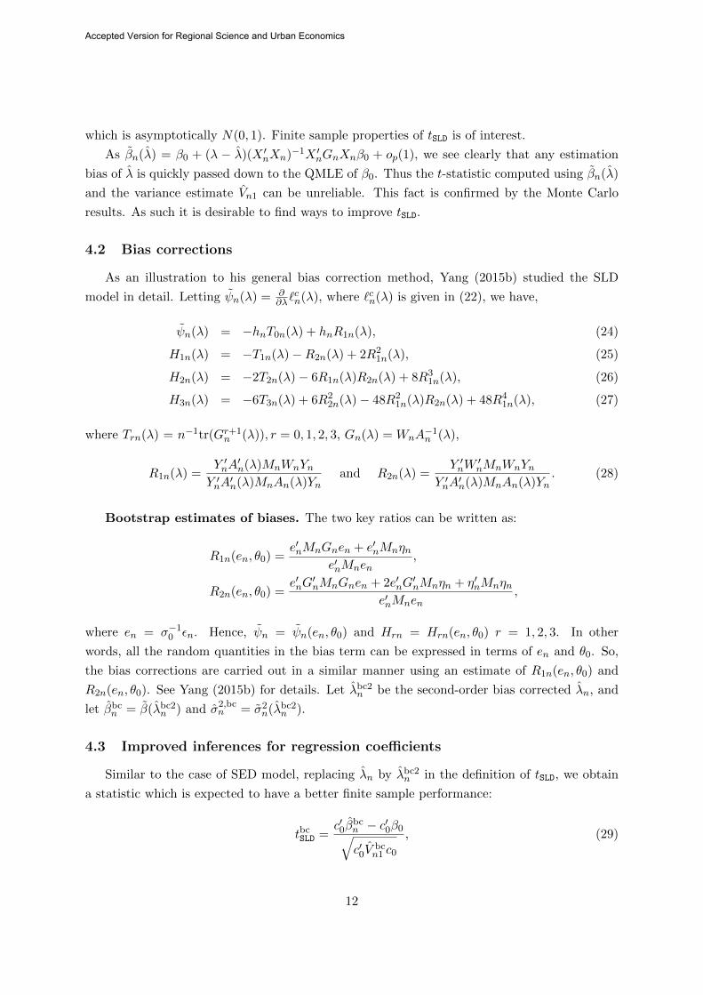
which is asymptotically N(0, 1). Finite sample properties of tSLD is of interest.
As βn(λ) = β0 + (λ − λ)(X ′nXn)−1X ′nGnXnβ0 + op(1), we see clearly that any estimation
bias of λ is quickly passed down to the QMLE of β0. Thus the t-statistic computed using βn(λ)
and the variance estimate Vn1 can be unreliable. This fact is confirmed by the Monte Carlo
results. As such it is desirable to find ways to improve tSLD.
4.2 Bias corrections
As an illustration to his general bias correction method, Yang (2015b) studied the SLD
model in detail. Letting ψn(λ) = ∂∂λ`
cn(λ), where `cn(λ) is given in (22), we have,
ψn(λ) = −hnT0n(λ) + hnR1n(λ), (24)
H1n(λ) = −T1n(λ)−R2n(λ) + 2R21n(λ), (25)
H2n(λ) = −2T2n(λ)− 6R1n(λ)R2n(λ) + 8R31n(λ), (26)
H3n(λ) = −6T3n(λ) + 6R22n(λ)− 48R2
1n(λ)R2n(λ) + 48R41n(λ), (27)
where Trn(λ) = n−1tr(Gr+1n (λ)), r = 0, 1, 2, 3, Gn(λ) = WnA
−1n (λ),
R1n(λ) =Y ′nA
′n(λ)MnWnYn
Y ′nA′n(λ)MnAn(λ)Yn
and R2n(λ) =Y ′nW
′nMnWnYn
Y ′nA′n(λ)MnAn(λ)Yn
. (28)
Bootstrap estimates of biases. The two key ratios can be written as:
R1n(en, θ0) =e′nMnGnen + e′nMnηn
e′nMnen,
R2n(en, θ0) =e′nG
′nMnGnen + 2e′nG
′nMnηn + η′nMnηn
e′nMnen,
where en = σ−10 εn. Hence, ψn = ψn(en, θ0) and Hrn = Hrn(en, θ0) r = 1, 2, 3. In other
words, all the random quantities in the bias term can be expressed in terms of en and θ0. So,
the bias corrections are carried out in a similar manner using an estimate of R1n(en, θ0) and
R2n(en, θ0). See Yang (2015b) for details. Let λbc2n be the second-order bias corrected λn, and
let βbcn = β(λbc2n ) and σ2,bcn = σ2n(λbc2n ).
4.3 Improved inferences for regression coefficients
Similar to the case of SED model, replacing λn by λbc2n in the definition of tSLD, we obtain
a statistic which is expected to have a better finite sample performance:
tbcSLD =c′0β
bcn − c′0β0√c′0V
bcn1 c0
, (29)
12
Accepted Version for Regional Science and Urban Economics

where V bcn1 is Vn1 evaluated at λbc2n , βbcn , σ2,bcn , γbcn , and κbcn . The last two are the estimates of
γ and κ, the skewness and excess kurtosis of εn,i involved in Vn1.
Now, to further improve tbcSLD, note that
βn − β0 = βn − β0 − (λn − λ0)(X ′nXn)−1X ′nGnXnβ0 − (λn − λ0)(X ′nXn)−1X ′nGnεn
= (X ′nXn)−1X ′n[εn − (a−1/2 + a−1)GnXnβ0 − a−1/2Gnεn
]+Op(n
−3/2).(30)
This leads immediately to a 2nd-order bias-corrected estimator βbc2n of β, and a second-order
expansion for Var(βn) as,
Var(βn) = (X ′nXn)−1X ′nVar[εn − (a−1/2 + a−1)GnXnβ0 − a−1/2Gnεn
]Xn(X ′nXn)−1 +O(n−2).
It is easy to see Var(βbc2n ) = Var(βn) + O(n−2). As in (30), an expansion can be carried out
for σ2n in terms of λn, leading to a 2nd-order bias-corrected estimator σ2,bc2n of σ2.3 Similarly, a
two-stage bootstrap procedure can be followed to give a consistent estimate of V = X ′nVar[εn−
(a−1/2 + a−1)GnXnβ0 − a−1/2Gnεn]Xn: first, run the algorithm BA-1 to give 2nd-order bias-
corrected estimators λbc2n , βbc2n and σ2,bc2n ; then update the residuals and run the algorithm
BA-1 again using the updated residuals to give a sequence of bootstrap values for V , and hence
the bootstrap estimate Var(βbc2n ) of Var(βn). The resulted 2nd-order bias-corrected t-statistic
is thus:
tbc2SLD =c′0β
bc2n − c′0β0√
c′0Var(βbc2n )c0
. (31)
4.4 Monte Carlo results
Finite sample performance of tSLD, tbcSLD and tbc2SLD is investigated under the following DGP:
Yn = λWnYn + ιnβ0 +X1nβ1 +X2nβ2 + εn,
where all the quantities are generated in a similar manner to those for the SED model. The
parameters for the Monte Carlo simulation are also set to be the same values as before.
Table 4.1 summarizes some empirical sizes of the tests tSLD, tbcSLD and tbc2SLD when used for
testing H0 : β1 = β2 under the Group Interaction scheme. From the results we see that (i)
as n increases, all tests converge in terms of sizes, (ii) it is indeed the case that the asymptotic
test tSLD can be very unreliable in the sense that it rejects the true H0 much too often than it
supposes to. The test tbc2SLD offers a huge reduction in size distortions, with the empirical sizes
getting close to their nominal levels faster than in the SED case. Nevertheless, when n = 50,
the results show that tbcSLD needs further improvements, and indeed the test tbc2SLD based on the
3Again, the estimators βbcn and βbc2
n do not differ much, and the estimators σ2,bcn and σ2,bc2
n do not differmuch. Hence in practical applications, one can use the simpler versions βbc
n and σ2,bcn .
13
Accepted Version for Regional Science and Urban Economics
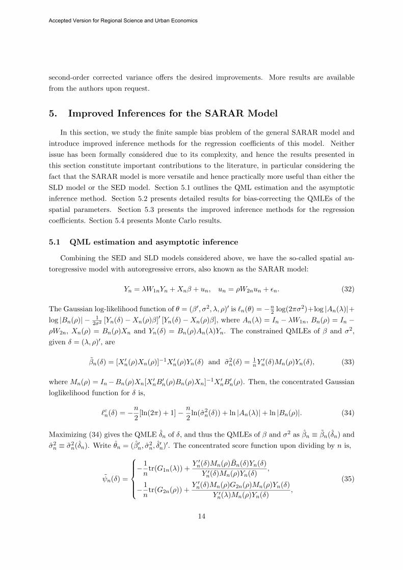
second-order corrected variance offers the desired improvements. More results are available
from the authors upon request.
5. Improved Inferences for the SARAR Model
In this section, we study the finite sample bias problem of the general SARAR model and
introduce improved inference methods for the regression coefficients of this model. Neither
issue has been formally considered due to its complexity, and hence the results presented in
this section constitute important contributions to the literature, in particular considering the
fact that the SARAR model is more versatile and hence practically more useful than either the
SLD model or the SED model. Section 5.1 outlines the QML estimation and the asymptotic
inference method. Section 5.2 presents detailed results for bias-correcting the QMLEs of the
spatial parameters. Section 5.3 presents the improved inference methods for the regression
coefficients. Section 5.4 presents Monte Carlo results.
5.1 QML estimation and asymptotic inference
Combining the SED and SLD models considered above, we have the so-called spatial au-
toregressive model with autoregressive errors, also known as the SARAR model:
Yn = λW1nYn +Xnβ + un, un = ρW2nun + εn. (32)
The Gaussian log-likelihood function of θ = (β′, σ2, λ, ρ)′ is `n(θ) = −n2 log(2πσ2)+log |An(λ)|+
log |Bn(ρ)| − 12σ2 [Yn(δ)−Xn(ρ)β]′ [Yn(δ)−Xn(ρ)β], where An(λ) = In − λW1n, Bn(ρ) = In −
ρW2n, Xn(ρ) = Bn(ρ)Xn and Yn(δ) = Bn(ρ)An(λ)Yn. The constrained QMLEs of β and σ2,
given δ = (λ, ρ)′, are
βn(δ) = [X ′n(ρ)Xn(ρ)]−1X ′n(ρ)Yn(δ) and σ2n(δ) = 1nY′n(δ)Mn(ρ)Yn(δ), (33)
where Mn(ρ) = In−Bn(ρ)Xn[X ′nB′n(ρ)Bn(ρ)Xn]−1X ′nB
′n(ρ). Then, the concentrated Gaussian
loglikelihood function for δ is,
`cn(δ) = −n2
[ln(2π) + 1]− n
2ln(σ2n(δ)) + ln |An(λ)|+ ln |Bn(ρ)|. (34)
Maximizing (34) gives the QMLE δn of δ, and thus the QMLEs of β and σ2 as βn ≡ βn(δn) and
σ2n ≡ σ2n(δn). Write θn = (β′n, σ2n, δ′n)′. The concentrated score function upon dividing by n is,
ψn(δ) =
− 1
ntr(G1n(λ)) +
Y ′n(δ)Mn(ρ)Bn(δ)Yn(δ)
Y ′n(δ)Mn(ρ)Yn(δ),
− 1
ntr(G2n(ρ)) +
Y ′n(δ)Mn(ρ)G2n(ρ)Mn(ρ)Yn(δ)
Y ′n(λ)Mn(ρ)Yn(δ),
(35)
14
Accepted Version for Regional Science and Urban Economics

where G1n(λ) = W1nA−1n (λ), G2n(ρ) = W2nB
−1n (ρ) and Bn(δ) = Bn(ρ)G1n(λ)B−1n (ρ).
Jin and Lee (2013) shows that under some regularity conditions, θn is asymptotically normal
with mean θ0 and asymptotic VC matrix Σ−1n ΓnΣ−1n , where
Σn =
1σ20X ′nB
′nBnXn 0 1
σ0X ′nB
′nµn 0
0 n2σ4
0
1σ20tr(Bn) 1
σ20tr(G2n)
1σ0µ′nBnXn
1σ20tr(Bn) µ′nµn + tr(Bs
nBn) tr(Gs2nBn)
0 1σ20tr(G2n) tr(Gs2nBn) tr(Gs2nG2n)
,
Γn =
0 γ
2σ30X ′nB
′nιn
γσ0X ′nB
′nbn
γσ0X ′nB
′ng2n
γ2σ3
0ι′nBnXn
nκ4σ4
0
κ2σ2
0tr(Bn) + γ
2σ20ι′nµn
κ2σ2
0tr(G2n)
γσ0b′nBnXn
κ2σ2
0tr(Bn) + γ
2σ20ι′nµn κb′nbn + 2γb′nµn κg′2nbn + γg′2nµn
γσ0g′2nBnXn
κ2σ2
0tr(G2n) κg′2nbn + γg′2nµn κg′2ng2n
+ Σn,
ιn, γ and κ are defined in the earlier sections, µn = σ−10 BnG1nXnβ0, bn = diag(Bn), g2n =
diag(G2n), Bsn = Bn + B′n and Gs2n = G2n +G′2n.
Letting Vn1 be the submatrix of Σ−1n ΓnΣ−1n corresponding to β and Vn1 be its estimate, an
asymptotic t-statistic for inferences for c′0β0 is thus,
tSARAR =c′0βn − c′0β0√
c′0Vn1c0
∼ N(0, 1). (36)
As indicated in the introduction, there is no formal treatment in the literature in terms of
the finite sample bias of the QML estimators of the SARAR model. Given the fact that the
QMLEs of the spatial parameters in the SED and SLD models can both be seriously biased,
there is a good reason to believe that they will remain to be biased when the spatial effects are
combined. Hence bias corrections for the QMLEs of the SARAR model would again be useful
in improving the inference methods for the model.
5.2 Bias corrections
Bias correction can be carried out as an application to the general method of bias correction
of Yang (2015b), for a vector of nonlinear estimators. To do so we need the higher-order partial
derivatives of ψn(δ), Hrn(δ) = ∇rψn(δ), r = 1, 2, 3, where the partial derivatives are obtained
sequentially and elementwise with respect to δ′. Define, Trn = tr(Gr1n(λ)) and Krn = tr(Gr2n(ρ)),
r = 0, 1, 2, 3. Also define the following quantities,
R1n(δ) =Y ′n(δ)Mn(ρ)Bn(δ)Yn(δ)
Y ′n(δ)Mn(ρ)Yn(δ),
R2n(δ) =Y ′n(δ)B′n(δ)Mn(ρ)Bn(δ)Yn(δ)
Y ′n(δ)Mn(ρ)Yn(δ),
15
Accepted Version for Regional Science and Urban Economics
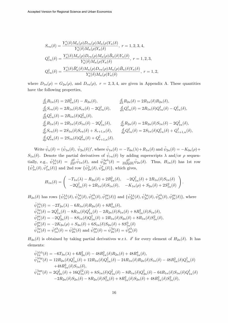
Srn(δ) =Y ′n(δ)Mn(ρ)Drn(ρ)Mn(ρ)Yn(δ)
Y ′n(δ)Mn(ρ)Yn(δ), r = 1, 2, 3, 4,
Q†rn(δ) =Y ′n(δ)Mn(ρ)Drn(ρ)Mn(ρ)Bn(δ)Yn(δ)
Y ′n(δ)Mn(ρ)Yn(δ), r = 1, 2, 3,
Q‡rn(δ) =Y ′n(δ)B′n(δ)Mn(ρ)Drn(ρ)Mn(ρ)Bn(δ)Yn(δ)
Y ′n(δ)Mn(ρ)Yn(δ), r = 1, 2,
where D1n(ρ) = G2n(ρ), and Drn(ρ), r = 2, 3, 4, are given in Appendix A. These quantities
have the following properties,
ddλR1n(δ) = 2R2
1n(δ)−R2n(δ), ddλR2n(δ) = 2R1n(δ)R2n(δ),
ddλSrn(δ) = 2R1n(δ)Srn(δ)− 2Q†rn(δ), d
dλQ†rn(δ) = 2R1n(δ)Q†rn(δ)−Q‡rn(δ),
ddλQ
‡rn(δ) = 2R1n(δ)Q‡rn(δ),
ddρR1n(δ) = 2R1n(δ)S1n(δ)− 2Q†1n(δ), d
dρR2n(δ) = 2R2n(δ)S1n(δ)− 2Q‡1n(δ),
ddρSrn(δ) = 2S1n(δ)Srn(δ) + Sr+1,n(δ), d
dρQ†rn(δ) = 2S1n(δ)Q†rn(δ) +Q†r+1,n(δ),
ddρQ
‡rn(δ) = 2S1n(δ)Q‡rn(δ) +Q‡r+1,n(δ).
Write ψn(δ) = (ψ1n(δ), ψ2n(δ))′, where ψ1n(δ) = −T0n(λ)+R1n(δ) and ψ2n(δ) = −K0n(ρ)+
S1n(δ). Denote the partial derivatives of ψrn(δ) by adding superscripts λ and/or ρ sequen-
tially, e.g., ψλλ1n (δ) = ∂2
∂λ2ψ1n(δ), and ψλρλ2n (δ) = ∂3
∂λ∂ρ∂λ ψ2n(δ). Thus, H1n(δ) has 1st row
ψλ1n(δ), ψρ1n(δ) and 2nd row ψλ2n(δ), ψρ2n(δ), which gives,
H1n(δ) =
(−T1n(λ)−R2n(δ) + 2R2
1n(δ), −2Q†1n(δ) + 2R1n(δ)S1n(δ)
−2Q†1n(δ) + 2R1n(δ)S1n(δ), −K1n(ρ) + S2n(δ) + 2S21n(δ)
).
H2n(δ) has rows ψλλ1n (δ), ψλρ1n(δ), ψρλ1n(δ), ψρρ1n(δ) and ψλλ2n (δ), ψλρ2n(δ), ψρλ2n(δ), ψρρ2n(δ), where
ψλλ1n (δ) = −2T2n(λ)− 6R1n(δ)R2n(δ) + 8R31n(δ),
ψλρ1n(δ) = 2Q‡1n(δ)− 8R1n(δ)Q†1n(δ)− 2R2n(δ)S1n(δ) + 8R21n(δ)S1n(δ),
ψρρ1n(δ) = −2Q†2n(δ)− 8S1n(δ)Q†1n(δ) + 2R1n(δ)S2n(δ) + 8R1n(δ)S21n(δ),
ψρρ2n(δ) = −2K2n(ρ) + S3n(δ) + 6S1n(δ)S2n(δ) + 8S31n(δ)
ψλρ1n(δ) = ψρλ1n(δ) = ψλλ2n (δ) and ψρρ1n(δ) = ψλρ2n(δ) = ψρλ2n(δ)
H3n(δ) is obtained by taking partial derivatives w.r.t. δ′ for every element of H2n(δ). It has
elements:
ψλλλ1n (δ) = −6T3n(λ) + 6R22n(δ)− 48R2
1n(δ)R2n(δ) + 48R41n(δ),
ψλλρ1n (δ) = 12R2n(δ)Q†1n(δ) + 12R1n(δ)Q‡1n(δ)− 24R1n(δ)R2n(δ)S1n(δ)− 48R21n(δ)Q†1n(δ)
+48R31n(δ)S1n(δ),
ψλρρ1n (δ) = 2Q‡2n(δ) + 16Q†21n(δ) + 8S1n(δ)Q‡1n(δ)− 8R1n(δ)Q†2n(δ)− 64R1n(δ)S1n(δ)Q†1n(δ)
−2R2n(δ)S2n(δ)− 8R2n(δ)S21n(δ) + 8R2
1n(δ)S2n(δ) + 48R21n(δ)S2
1n(δ),
16
Accepted Version for Regional Science and Urban Economics
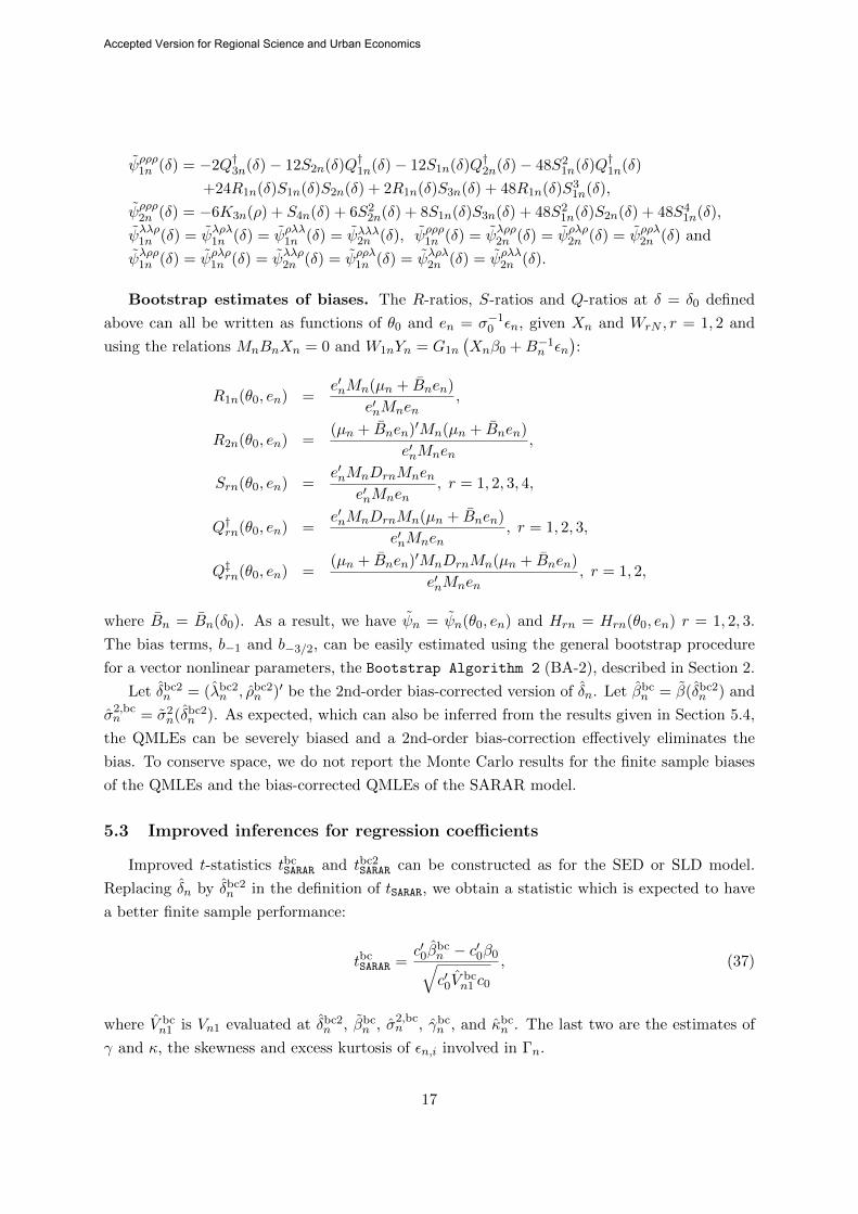
ψρρρ1n (δ) = −2Q†3n(δ)− 12S2n(δ)Q†1n(δ)− 12S1n(δ)Q†2n(δ)− 48S21n(δ)Q†1n(δ)
+24R1n(δ)S1n(δ)S2n(δ) + 2R1n(δ)S3n(δ) + 48R1n(δ)S31n(δ),
ψρρρ2n (δ) = −6K3n(ρ) + S4n(δ) + 6S22n(δ) + 8S1n(δ)S3n(δ) + 48S2
1n(δ)S2n(δ) + 48S41n(δ),
ψλλρ1n (δ) = ψλρλ1n (δ) = ψρλλ1n (δ) = ψλλλ2n (δ), ψρρρ1n (δ) = ψλρρ2n (δ) = ψρλρ2n (δ) = ψρρλ2n (δ) and
ψλρρ1n (δ) = ψρλρ1n (δ) = ψλλρ2n (δ) = ψρρλ1n (δ) = ψλρλ2n (δ) = ψρλλ2n (δ).
Bootstrap estimates of biases. The R-ratios, S-ratios and Q-ratios at δ = δ0 defined
above can all be written as functions of θ0 and en = σ−10 εn, given Xn and WrN , r = 1, 2 and
using the relations MnBnXn = 0 and W1nYn = G1n
(Xnβ0 +B−1n εn
):
R1n(θ0, en) =e′nMn(µn + Bnen)
e′nMnen,
R2n(θ0, en) =(µn + Bnen)′Mn(µn + Bnen)
e′nMnen,
Srn(θ0, en) =e′nMnDrnMnen
e′nMnen, r = 1, 2, 3, 4,
Q†rn(θ0, en) =e′nMnDrnMn(µn + Bnen)
e′nMnen, r = 1, 2, 3,
Q‡rn(θ0, en) =(µn + Bnen)′MnDrnMn(µn + Bnen)
e′nMnen, r = 1, 2,
where Bn = Bn(δ0). As a result, we have ψn = ψn(θ0, en) and Hrn = Hrn(θ0, en) r = 1, 2, 3.
The bias terms, b−1 and b−3/2, can be easily estimated using the general bootstrap procedure
for a vector nonlinear parameters, the Bootstrap Algorithm 2 (BA-2), described in Section 2.
Let δbc2n = (λbc2n , ρbc2n )′ be the 2nd-order bias-corrected version of δn. Let βbcn = β(δbc2n ) and
σ2,bcn = σ2n(δbc2n ). As expected, which can also be inferred from the results given in Section 5.4,
the QMLEs can be severely biased and a 2nd-order bias-correction effectively eliminates the
bias. To conserve space, we do not report the Monte Carlo results for the finite sample biases
of the QMLEs and the bias-corrected QMLEs of the SARAR model.
5.3 Improved inferences for regression coefficients
Improved t-statistics tbcSARAR and tbc2SARAR can be constructed as for the SED or SLD model.
Replacing δn by δbc2n in the definition of tSARAR, we obtain a statistic which is expected to have
a better finite sample performance:
tbcSARAR =c′0β
bcn − c′0β0√c′0V
bcn1 c0
, (37)
where V bcn1 is Vn1 evaluated at δbc2n , βbcn , σ2,bcn , γbcn , and κbcn . The last two are the estimates of
γ and κ, the skewness and excess kurtosis of εn,i involved in Γn.
17
Accepted Version for Regional Science and Urban Economics
In order to further improve tbcSARAR, note that given βn = βn(δ0), let β(r)n be the rth derivative
with respect to δ′0, r = 1, 2. Also define Fn(ρ) = [X ′nB′n(ρ)Bn(ρ)Xn]−1X ′nB
′n(ρ)Bn(ρ) where
we have βn(δ) = Fn(ρ)An(λ)Yn and F(r)n = F
(r)n (ρ0) is the rth derivative with respect to
δ′0, r = 1, 2. Assuming that E(β(r)n ) exists and that β
(r)n − E(β
(r)n ) = Op(n
−1/2), r = 1, 2, by a
Taylor expansion, we have,
βn(δn)− β0 = βn − β0 + β(1)n (δn − δ0) + 12 β
(2)n [(δn − δ0)⊗ (δn − δ0)] +Op(n
−3/2),
= b0n + E(β(1)n )(a−1/2 + a−1) + b1na−1/2 + 12E(β
(2)n )(a−1/2 ⊗ a−1/2) +Op(n
−3/2),
where b0n = FnB−1n εn, b1n = (−FnG1nB
−1n εn, F
(1)n B−1n εn), E(β
(1)n ) = (−FnG1nXnβ0, F
(1)n Xnβ0)
and E(β(2)n ) = (0k×1, −F
(1)n G1nXnβ0, −F (1)
n G1nXnβ0, F(2)n Xnβ0). The expressions for F
(1)n and
F(2)n are given in Appendix A. This leads to a second order expansion for Var(βn) or Var(βbc2n ):
Var(βbc2n ) = Var[b0n + E(β(1)n )(a−1/2 + a−1) + b1na−1/2 + 12E(β
(2)n )(a−1/2 ⊗ a−1/2)] +Op(n
−2),
where a−1/2 = Ωnψn and a−1 = ΩnH1na−1/2+
12ΩnE(H2n)(a−1/2⊗a−1/2) = Ωnψn+ΩnH1nΩnψn+
12ΩnE(H2n)[(Ωnψn)⊗(Ωnψn)] = Ωnψn+Ωn(ψ′n⊗H1n)vec(Ωn)+ 1
2ΩnE(H2n)(Ωn⊗Ωn)(ψn⊗ψn),
(see Yang, 2015b). As for the two simpler models, one can easily obtain the 2nd-order bias-
corrected estimators βbc2n and σ2,bc2n , but again Monte Carlo results (not reported for brevity)
show that they do not differ much from the corresponding ‘plug-in’ estimators. A similar two
stage bootstrap procedure as given in Section 3, but based on the algorithm BA-2 presented in
Section 2, can be applied to obtain an estimate of this variance term, Var(βbc2n ). We have a
second order bias corrected t-statistic as follows:
tbc2SARAR =c′0β
bc2n − c′0β0√
c′0Var(βbc2n )c0
. (38)
5.4 Monte Carlo results
The methods for bias-correction and for improved inferences introduced above for the
SARAR model are investigated for their finite sample performance under the following DGP:
Yn = λW1nYn + ιnβ0 +X1nβ1 +X2nβ2 + un, un = ρW2nun + εn,
where all the quantities are generated in a similar manner to those for the SED model. The
two spatial weight matrices are taken to be the same. The parameters are set to be the same
as before, where λ and ρ both take values from −0.5,−0.25, 0, 0.25, 0.5.We focus on the finite sample performance of the three tests tSARAR, t
bcSARAR and tbc2SARAR. The
results for the finite sample bias of the QMLEs are available from the authors upon request.
Tables 5.1-5.3 report empirical sizes of tSARAR, tbcSARAR and tbc2SARAR when used for testingH0 : β1 = β2,
18
Accepted Version for Regional Science and Urban Economics
under the Group Interaction spatial layouts described in Appendix B. Similar conclusions are
drawn from the Monte Carlo results for the SARAR model as those for the two sub models
considered in the earlier sections: (i) as n increases, all tests converge in terms of sizes, (ii)
the asymptotic test tSARAR remains unreliable in the sense it rejects the true H0 much too often
than it supposes to, (iii) the test tbcSARAR offers immediate reduction in size distortions, and (iv)
tbc2SARAR generally offers further improvements. Furthermore, like the asymptotic test for the SED
model, tSARAR can have a size distortion that is very persistent, having values that are at least
24% even when n = 500. The results (unreported to conserve space) under Rook and Queen
Contiguity show similar patterns, but the differences are of a lesser degree due to the weaker
spatial dependence (less number of neighbours) under these two spatial layouts.
6. Conclusions
This paper considers inference problems for the regression coefficients β in linear regression
models with spatial dependence, where the estimation of the spatial parameters may incur
severe bias. It is shown that while the existence of spatial dependence does not have a big
impact on the point estimation of the regression coefficients in terms of consistency and bias (in
particular after bias-correcting the spatial estimators), it can have a huge impact on the usual
t-statistics for β. We propose simple ways to correct the t-statistics, and the resulted 2nd-order
corrected t-statistics perform superbly. Considering the effectiveness and the simplicity of the
proposed methods, they are recommended for practical applications.
Central to the proposed inference methods for regression coefficients in this paper is the
general bias-correction methods for nonlinear estimators proposed in Yang (2015b). Thus, the
proposed methods have a great potential to be extended to more advanced models such as
higher-order SARAR models, spatial panel data models, dynamic panel data models, nonlinear
spatial regression models and nonlinear spatial panel data models. They are equally applicable
to non-spatial models as well. Among these, the extension to a higher-order SARAR incurs
only some extra algebra, and all methods go through in a straightforward manner.
The classical approach to the problem considered in this paper is to directly bootstrap the
original t-statistic to give asymptotically refined approximations to the finite sample critical
values, taking advantage of the underlining statistic being asymptotically pivotal. However,
bootstrapping a Wald-type or a likelihood ratio statistic requires the reestimation of all param-
eters in every bootstrap iteration, and thus is computationally much more demanding compared
to our approach, in particular when the model contains more nonlinear parameters that needed
to be estimated through numerical optimization (see Yang 2015a for some related works and
discussions). Nevertheless, it would be interesting as a future research to compare the two
approaches, considering the fact that the direct approach is algebraically simpler.4
4We thank a referee for raising this issue.
19
Accepted Version for Regional Science and Urban Economics
Appendix A: Additional Quantities for Bias Corrections
For the SED model, the full expressions for Djn(ρ), j = 2, 3, 4, required in the expressions
of Rjn(ρ) in (15), for up to third-order bias corrections are:
D2n(ρ) = 2Gn(ρ)Pn(ρ)Gn(ρ) +Gn(ρ)Pn(ρ)G′n(ρ)−G′n(ρ)Mn(ρ)Gn(ρ),
D3n(ρ) = D2n(ρ) +Gn(ρ)Pn(ρ)D2n(ρ) +D2n(ρ)Pn(ρ)G′n(ρ)
−G′n(ρ)Mn(ρ)D2n(ρ)−D2n(ρ)Mn(ρ)Gn(ρ),
D4n(ρ) = D3n(ρ) +Gn(ρ)Pn(ρ)D3n(ρ) +D3n(ρ)Pn(ρ)G′n(ρ)
−G′n(ρ)Mn(ρ)D3n(ρ)−D3n(ρ)Mn(ρ)Gn(ρ),
where Pn(ρ) = In −Mn(ρ) and Djn(ρ) = ddρDjn(ρ), j = 2, 3. Note that a predictable pattern
emerges from D3n(ρ) onwards. Using the fact that ddρG
in = Gi+1
n for i = 1, 2, . . ., we have,
D2n(ρ) = 2G2n(ρ)Pn(ρ)Gn(ρ)− 2Gn(ρ)Mn(ρ)Gn(ρ) + 2Gn(ρ)Pn(ρ)G2
n(ρ)
+G2n(ρ)Pn(ρ)G′n(ρ)−Gn(ρ)Mn(ρ)G′n(ρ) +Gn(ρ)Pn(ρ)G
′2n (ρ)
−G′2n (ρ)Mn(ρ)Gn(ρ)−G′n(ρ)Mn(ρ)Gn(ρ)−G′n(ρ)Mn(ρ)G2n(ρ),
D3n(ρ) = G′3n (ρ)Mn(ρ)Gn(ρ) + 2G
′2n (ρ)Mn(ρ)Gn(ρ) + 2G
′2n (ρ)Mn(ρ)G2
n(ρ)
+G′n(ρ)Mn(ρ)Gn(ρ) + 2G′n(ρ)Mn(ρ)G2n(ρ) +G′n(ρ)Mn(ρ)G3
n(ρ)
−2G3n(ρ)Pn(ρ)Gn(ρ) + 4G2
n(ρ)Mn(ρ)Gn(ρ)− 4G2n(ρ)Pn(ρ)G2
n(ρ)
+2Gn(ρ)Mn(ρ)Gn(ρ) + 4Gn(ρ)Mn(ρ)G2n(ρ)− 2Gn(ρ)Pn(ρ)G3
n(ρ)
−G3n(ρ)Pn(ρ)G′n(ρ) + 2G2(ρ)Mn(ρ)G′n(ρ)− 2G2
n(ρ)Pn(ρ)G′2n (ρ)
+Gn(ρ)Mn(ρ)G′n(ρ) + 2Gn(ρ)Mn(ρ)G′2n (ρ)−Gn(ρ)Pn(ρ)G
′3n (ρ),
Mn(ρ) = Pn(ρ)G′n(ρ)Mn(ρ) +Mn(ρ)Gn(ρ)Pn(ρ),
Mn(ρ) = 2Pn(ρ)G′n(ρ)Pn(ρ)G′n(ρ)Mn(ρ) + 2Pn(ρ)G′n(ρ)Mn(ρ)Gn(ρ)Pn(ρ)
+2Mn(ρ)Gn(ρ)Pn(ρ)Gn(ρ)Pn(ρ)− 2Mn(ρ)Gn(ρ)Pn(ρ)G′n(ρ)Mn(ρ).
The expressions for F(r)n = dr
dρr0Fn(ρ0), r = 1, 2 are:
F(1)n = FnB
−1n GsnBn(XnFn − In), where Gsn = Gn +G′n
F(2)n = F
(1)n B−1n GsnBn(XnFn−In)+FnB
−1n (Gs2n −2G′nGn)Bn(XnFn−In)+FnB
−1n GsnBnXnF
(1)n
For the SARAR model, the full expressions for Djn(ρ), j = 2, 3, 4 and F(r)n , r = 1, 2
follow a similar pattern as in the quantities for the SED model with the exception that Gn(ρ)
in the SED must now be replaced with G2n(ρ).
20
Accepted Version for Regional Science and Urban Economics
Appendix B: Settings of Monte Carlo Experiments
Spatial Weight Matrix: We use three different methods for generating the spatial weight
matrix Wn: (i) Rook contiguity, (ii) Queen contiguity, and (iii) Group Interaction, with
details given in Yang (2015b). The degree of spatial dependence specified by layouts (i) and (ii)
are fixed while in (iii) it grows with the increase in sample size. This is attained by allowing
for the number of groups, k, for each sample to be directly related to n. We have considered
k = n0.5 and k = n0.65, where k is the number of groups for each n and hence the degree of
spatial dependence indicated by the average group size is m = n/k. The actual sizes of the
groups are generated from a discrete uniform distribution from .5m to 1.5m.
Regressors: The fixed regressors are generated by REG1: x1i, x2iiid∼ N(0, 1)/
√2 when
Rook or Queen contiguity is followed; and according to either REG1 or REG2: x1,ir, x2,iriid∼
(2zr+zir)/√
10, where, (zr, zir)iid∼ N(0, 1) when group interaction scheme is followed. The REG2
scheme gives non-iid regressors where the group means of the regressors’ values are different,
see Lee (2004). Note that both schemes give a signal-to-noise ratio of 1 when β1 = β2 = σ = 1.
Error Distribution: To generate εn = σen, three DGPs are considered: DGP1: en,i are
iid standard normal, DGP2: en,i are iid standardized normal mixture with 10% of values from
N(0, 4) and the remaining from N(0, 1), and DGP3: en,i iid standardized log-normal with
parameters 0 and 1. Thus, the error distribution from DGP2 is leptokurtic, and that of DGP3 is
both skewed and leptokurtic.
21
Accepted Version for Regional Science and Urban Economics

References
Anselin, L., 1988. Spatial Econometrics: Methods and Models. The Netherlands: Kluwer
Academic Publishers.
Anselin, L., 2001. Spatial Econometrics. A Companion to Theoretical Econometrics, edited by
Badi H. Baltagi. Blackwell Publishing.
Anselin, L., Bera, A. K., 1998. Spatial dependence in linear regression models with an intro-
duction to spatial econometrics. In: Handbook of Applied Economic Statistics, edited by
Aman Ullah and David E. A. Giles. New York: Marcel Dekker.
Baltagi, B., Yang, Z. L., 2013a. Standardized LM tests for spatial error dependence in linear
or panel regressions. The Econometrics Journal 16 103-134.
Baltagi, B., Yang, Z. L., 2013b. Heteroskedasticity and non-normality robust LM tests of
spatial dependence. Regional Science and Urban Economics 43, 725-739.
Bao, Y., 2013. Finite sample bias of QMLE in spatial autoregressive models. Econometric
Theory 29 68-88.
Bao, Y., Ullah, A., 2007. Finite sample properties of maximum likelihood estimator in spatial
models. Journal of Econometrics 137, 396-413.
Jin, F., Lee, L. F., 2013. Cox-type tests for competing spatial autoregressive models with
spatial autoregressive disturbances Regional Science and Urban Economics. 43 590-616.
Lee, L. F., 2004. Asymptotic distributions of quasi-maximum likelihood estimators for spatial
autoregressive models. Econometrica 72, 1899-1925.
Liu S. F., Yang Z. L., 2015. Asymptotic Distribution and Finite-Sample Bias Correction of
QML Estimators for Spatial Error Dependence Model. Econometrics 3, 376-411.
Rilstone, P., Srivastava, V. K., Ullah, A., 1996. The second-order bias and mean squared error
of nonlinear estimators. Journal of Econometrics 75, 369-395.
Robinson, P. M., Rossi, F., 2014a. Refined tests for spatial correlation. Econometric Theory,
forthcoming.
Robinson, P. M., Rossi, F., 2014b. Improved Lagrange multiplier tests in spatial autoregres-
sions. Econometrics Journal 17, 139-164.
Yang, Z. L., 2010. A robust LM test for spatial error components. Regional Science and Urban
Economics 40, 299-310.
Yang, Z. L., 2015a. LM tests of spatial dependence based on bootstrap critical values. Journal
of Econometrics 185, 33-39.
Yang, Z. L., 2015b. A general method for third order bias and variance corrections on a
non-linear estimator. Journal of Econometrics 186, 178-200.
22
Accepted Version for Regional Science and Urban Economics

Table 3.1 Empirical Sizes: Two-Sided Tests of H0 : β1 = β2 in SED ModelGroup Interaction, REG2, σ = 1; Test: 1 = tSED, 2 = tbcSED, 3 = tbc2SED
ρ Test 10% 5% 1% 10% 5% 1% 10% 5% 1% 10% 5% 1% 10% 5% 1% 10% 5% 1%Normal Errors Normal Mixture Lognormal Normal Errors Normal Mixture Lognormal
n = 50 n = 200.50 1 .232 .169 .088 .239 .173 .092 .237 .167 .086 .128 .073 .020 .139 .076 .024 .125 .068 .018
2 .132 .078 .029 .136 .083 .032 .132 .079 .029 .107 .057 .014 .117 .060 .016 .109 .059 .0143 .113 .066 .024 .116 .072 .028 .112 .068 .024 .100 .053 .012 .108 .057 .014 .102 .052 .012
.25 1 .252 .185 .102 .254 .188 .104 .255 .186 .100 .153 .092 .030 .138 .080 .026 .141 .084 .0282 .133 .083 .038 .132 .083 .037 .136 .082 .035 .114 .060 .018 .116 .063 .017 .109 .058 .0153 .117 .076 .034 .120 .075 .033 .121 .073 .031 .108 .056 .016 .109 .057 .014 .101 .053 .013
.00 1 .259 .195 .105 .259 .193 .105 .265 .194 .104 .152 .093 .035 .157 .094 .034 .153 .098 .0342 .134 .084 .036 .136 .086 .040 .138 .085 .035 .110 .060 .018 .114 .062 .017 .116 .066 .0193 .125 .077 .034 .125 .079 .037 .126 .077 .033 .104 .056 .017 .108 .058 .016 .108 .060 .017
-.25 1 .270 .195 .110 .263 .193 .105 .267 .196 .108 .161 .101 .039 .166 .102 .037 .160 .099 .0392 .141 .093 .047 .140 .091 .042 .146 .092 .040 .114 .063 .020 .114 .064 .018 .111 .065 .0203 .135 .088 .044 .132 .086 .040 .137 .085 .037 .109 .060 .018 .109 .060 .018 .108 .062 .019
-.50 1 .260 .191 .102 .258 .189 .098 .262 .193 .103 .166 .102 .037 .167 .107 .038 .168 .106 .0392 .142 .096 .043 .145 .094 .044 .147 .096 .043 .112 .062 .017 .119 .064 .020 .118 .066 .0203 .136 .099 .033 .139 .099 .031 .141 .099 .031 .109 .060 .010 .104 .060 .011 .102 .061 .011
n = 100 n = 500.50 1 .164 .103 .042 .170 .107 .042 .172 .106 .041 .123 .065 .018 .124 .067 .017 .120 .066 .017
2 .124 .070 .023 .128 .074 .021 .129 .072 .018 .105 .054 .014 .109 .055 .013 .108 .055 .0133 .113 .062 .019 .115 .064 .017 .115 .062 .015 .101 .053 .012 .104 .051 .012 .103 .052 .010
.25 1 .190 .126 .054 .192 .127 .053 .192 .126 .055 .132 .074 .022 .126 .070 .019 .130 .072 .0212 .128 .076 .023 .127 .075 .021 .130 .074 .025 .107 .056 .015 .104 .053 .014 .107 .054 .0153 .117 .068 .020 .117 .067 .019 .119 .067 .020 .104 .053 .010 .101 .051 .010 .102 .052 .011
.00 1 .200 .133 .058 .197 .128 .056 .204 .133 .058 .132 .077 .024 .136 .077 .024 .134 .075 .0242 .124 .070 .024 .123 .072 .023 .126 .073 .025 .105 .057 .015 .107 .056 .014 .107 .056 .0153 .116 .064 .021 .114 .066 .021 .119 .070 .023 .103 .050 .011 .105 .051 .010 .103 .051 .010
-.25 1 .201 .132 .060 .204 .137 .059 .199 .129 .057 .135 .077 .023 .135 .076 .021 .133 .076 .0212 .124 .072 .027 .123 .071 .024 .117 .068 .023 .104 .056 .014 .104 .053 .013 .105 .056 .0133 .116 .067 .026 .115 .066 .022 .109 .063 .022 .102 .051 .011 .102 .050 .012 .102 .054 .013
-.50 1 .198 .137 .058 .195 .130 .057 .203 .133 .058 .137 .077 .023 .134 .077 .024 .133 .077 .0242 .118 .068 .024 .117 .069 .026 .120 .071 .025 .105 .058 .014 .100 .054 .015 .101 .055 .0133 .110 .065 .021 .111 .060 .020 .115 .068 .021 .104 .051 .010 .100 .051 .011 .101 .051 .010
23
Accepted Version for Regional Science and Urban Economics

Table 4.1 Empirical Sizes: Two-Sided Tests of H0 : β1 = β2 in SLD ModelGroup Interaction, REG2, σ = 1; Test: 1 = tSLD, 2 = tbcSLD, 3 = tbc2SLD
ρ Test 10% 5% 1% 10% 5% 1% 10% 5% 1% 10% 5% 1% 10% 5% 1% 10% 5% 1%Normal Errors Normal Mixture Lognormal Normal Errors Normal Mixture Lognormal
n = 50 n = 200.50 1 .161 .095 .028 .162 .095 .029 .174 .120 .058 .109 .057 .013 .113 .059 .014 .125 .068 .019
2 .113 .062 .016 .117 .068 .017 .142 .098 .049 .102 .051 .012 .104 .052 .011 .114 .061 .0163 .095 .045 .010 .100 .045 .010 .100 .054 .014 .093 .048 .011 .098 .048 .011 .100 .050 .010
.25 1 .156 .095 .028 .160 .095 .026 .171 .107 .041 .115 .060 .013 .111 .056 .012 .123 .063 .0142 .113 .062 .014 .117 .065 .015 .139 .085 .033 .106 .055 .012 .103 .050 .011 .112 .054 .0123 .095 .044 .009 .093 .045 .010 .098 .050 .012 .100 .049 .010 .097 .046 .010 .100 .047 .010
.00 1 .158 .097 .030 .157 .090 .028 .139 .073 .021 .115 .056 .012 .115 .061 .014 .114 .061 .0152 .115 .065 .018 .116 .062 .017 .110 .060 .015 .106 .051 .010 .104 .053 .011 .105 .054 .0123 .100 .048 .012 .093 .049 .012 .099 .053 .015 .099 .046 .009 .099 .048 .010 .098 .049 .010
-.25 1 .163 .096 .033 .161 .099 .032 .122 .067 .019 .112 .057 .015 .112 .058 .012 .111 .058 .0112 .117 .068 .020 .124 .069 .020 .100 .049 .012 .105 .054 .013 .105 .053 .010 .108 .055 .0113 .095 .052 .014 .102 .053 .015 .100 .050 .010 .100 .049 .012 .100 .050 .010 .103 .052 .009
-.50 1 .167 .100 .033 .161 .099 .034 .113 .062 .017 .119 .065 .016 .108 .056 .012 .105 .057 .0142 .124 .069 .020 .126 .074 .022 .094 .046 .012 .108 .058 .013 .107 .056 .013 .099 .052 .0113 .099 .055 .016 .106 .051 .015 .103 .050 .011 .099 .051 .011 .099 .049 .011 .100 .051 .011
n = 100 n = 500.50 1 .131 .070 .018 .127 .067 .017 .133 .077 .027 .106 .053 .011 .111 .057 .014 .107 .056 .012
2 .105 .055 .013 .103 .051 .011 .117 .066 .023 .101 .048 .009 .104 .051 .012 .102 .052 .0113 .098 .054 .010 .099 .049 .018 .093 .048 .010 .099 .050 .010 .098 .048 .011 .097 .048 .010
.25 1 .127 .068 .019 .130 .073 .019 .145 .087 .024 .110 .060 .012 .109 .057 .013 .109 .054 .0112 .103 .052 .014 .109 .056 .014 .120 .069 .018 .103 .055 .011 .100 .051 .010 .104 .050 .0103 .096 .049 .010 .093 .050 .010 .095 .046 .009 .098 .050 .010 .099 .050 .009 .099 .049 .010
.00 1 .133 .070 .019 .130 .071 .017 .128 .073 .018 .107 .055 .012 .109 .058 .012 .108 .055 .0132 .105 .054 .013 .109 .057 .012 .111 .059 .013 .101 .051 .011 .102 .053 .010 .101 .051 .0123 .100 .050 .010 .099 .050 .009 .099 .052 .011 .099 .050 .010 .097 .049 .009 .100 .049 .011
-.25 1 .133 .071 .020 .134 .077 .021 .130 .065 .013 .103 .052 .014 .107 .054 .012 .105 .054 .0122 .109 .054 .014 .112 .060 .015 .110 .051 .009 .097 .048 .012 .100 .049 .011 .099 .050 .0103 .100 .046 .011 .099 .047 .010 .103 .049 .010 .099 .050 .011 .099 .049 .010 .099 .050 .010
-.50 1 .128 .071 .017 .132 .074 .018 .113 .057 .012 .105 .056 .013 .108 .056 .011 .107 .054 .0112 .106 .057 .013 .112 .060 .012 .094 .044 .008 .098 .052 .011 .102 .050 .009 .100 .050 .0093 .099 .050 .010 .099 .052 .011 .100 .049 .010 .099 .050 .010 .099 .049 .010 .100 .049 .009
24
Accepted Version for Regional Science and Urban Economics

Table 5.1 Empirical Sizes: Two-Sided Tests of H0 : β1 = β2 in SARAR ModelGroup Interaction, REG2, σ = 1, λ = 0.5; Test: 1 = tSARAR, 2 = tbcSARAR, 3 = tbc2SARAR
ρ Test 10% 5% 1% 10% 5% 1% 10% 5% 1% 10% 5% 1% 10% 5% 1% 10% 5% 1%Normal Errors Normal Mixture Lognormal Normal Errors Normal Mixture Lognormal
n = 50 n = 200.50 1 .197 .115 .040 .201 .122 .044 .197 .122 .040 .141 .078 .022 .140 .082 .028 .131 .078 .021
2 .120 .068 .020 .123 .073 .023 .146 .084 .028 .113 .056 .014 .117 .061 .017 .116 .061 .0153 .115 .062 .017 .119 .068 .023 .128 .074 .024 .105 .050 .011 .107 .056 .016 .106 .052 .013
.25 1 .191 .109 .031 .180 .110 .031 .183 .109 .035 .147 .085 .025 .152 .089 .028 .150 .083 .0252 .118 .067 .020 .116 .069 .022 .120 .066 .021 .108 .056 .012 .112 .061 .012 .111 .058 .0123 .109 .061 .016 .103 .058 .019 .103 .055 .017 .100 .050 .009 .102 .054 .011 .101 .051 .010
.00 1 .191 .110 .031 .177 .099 .028 .191 .114 .037 .150 .089 .026 .137 .075 .016 .138 .084 .0202 .111 .054 .015 .100 .054 .016 .117 .065 .021 .104 .055 .012 .116 .061 .014 .124 .066 .0173 .098 .047 .012 .095 .046 .013 .100 .055 .018 .097 .050 .010 .102 .051 .010 .105 .052 .012
-.25 1 .173 .100 .025 .170 .096 .027 .184 .108 .033 .158 .093 .030 .131 .074 .018 .120 .062 .0142 .094 .048 .011 .098 .049 .016 .111 .059 .020 .108 .054 .013 .123 .068 .019 .118 .066 .0173 .108 .048 .009 .108 .051 .013 .090 .047 .016 .099 .049 .012 .102 .055 .010 .095 .054 .010
-.50 1 .182 .104 .030 .162 .085 .023 .177 .100 .034 .127 .072 .020 .120 .061 .013 .119 .063 .0132 .097 .049 .013 .085 .043 .010 .102 .059 .019 .115 .066 .017 .122 .063 .015 .135 .074 .0193 .100 .048 .011 .091 .052 .009 .092 .046 .014 .105 .060 .013 .095 .046 .009 .091 .052 .009
n = 100 n = 500.50 1 .169 .099 .027 .163 .097 .029 .171 .103 .031 .124 .068 .018 .126 .070 .017 .124 .073 .018
2 .115 .058 .014 .122 .064 .017 .115 .059 .016 .102 .053 .013 .107 .053 .011 .106 .056 .0113 .101 .049 .013 .107 .057 .015 .105 .055 .013 .098 .049 .012 .100 .049 .010 .100 .050 .010
.25 1 .165 .094 .029 .172 .101 .028 .163 .095 .030 .130 .073 .023 .134 .073 .020 .130 .074 .0182 .106 .054 .012 .116 .056 .011 .111 .056 .013 .105 .056 .015 .106 .057 .014 .101 .053 .0123 .095 .045 .010 .101 .047 .009 .098 .049 .011 .099 .052 .014 .100 .053 .013 .099 .049 .010
.00 1 .177 .103 .031 .176 .098 .032 .165 .100 .035 .138 .075 .021 .135 .072 .019 .133 .076 .0202 .105 .054 .012 .102 .052 .013 .105 .056 .014 .106 .055 .013 .099 .052 .009 .106 .054 .0123 .093 .046 .011 .099 .048 .011 .095 .051 .013 .103 .053 .011 .099 .049 .009 .101 .053 .010
-.25 1 .170 .100 .027 .164 .095 .029 .170 .098 .029 .131 .074 .020 .135 .077 .022 .132 .075 .0222 .096 .047 .010 .097 .048 .010 .102 .048 .011 .101 .055 .013 .102 .053 .012 .098 .053 .0113 .095 .054 .011 .099 .050 .009 .099 .052 .010 .096 .051 .012 .099 .051 .011 .100 .051 .010
-.50 1 .158 .091 .026 .151 .086 .022 .145 .087 .024 .128 .071 .018 .144 .076 .022 .129 .072 .0192 .090 .046 .010 .091 .044 .010 .091 .048 .011 .094 .046 .011 .107 .054 .014 .093 .050 .0113 .090 .054 .009 .099 .047 .009 .098 .052 .009 .092 .045 .011 .103 .051 .013 .099 .050 .010
25
Accepted Version for Regional Science and Urban Economics

Table 5.2 Empirical Sizes: Two-Sided Tests of H0 : β1 = β2 in SARAR ModelGroup Interaction, REG2, σ = 1, λ = 0.0; Test: 1 = tSARAR, 2 = tbcSARAR, 3 = tbc2SARAR
ρ Test 10% 5% 1% 10% 5% 1% 10% 5% 1% 10% 5% 1% 10% 5% 1% 10% 5% 1%Normal Errors Normal Mixture Lognormal Normal Errors Normal Mixture Lognormal
n = 50 n = 200.50 1 .186 .107 .027 .196 .127 .050 .188 .114 .037 .134 .079 .020 .132 .066 .019 .135 .074 .018
2 .130 .073 .020 .123 .076 .027 .132 .079 .027 .111 .058 .014 .107 .055 .013 .116 .061 .0133 .128 .068 .017 .113 .071 .025 .118 .069 .023 .101 .052 .012 .098 .049 .010 .104 .053 .010
.25 1 .199 .125 .047 .187 .113 .039 .204 .130 .048 .140 .083 .023 .143 .086 .029 .153 .087 .0252 .115 .064 .021 .126 .071 .018 .111 .065 .020 .117 .066 .017 .107 .060 .016 .108 .058 .0153 .110 .061 .020 .112 .061 .015 .108 .062 .019 .107 .060 .014 .098 .053 .014 .096 .050 .013
.00 1 .184 .110 .034 .184 .107 .033 .203 .126 .043 .157 .093 .029 .155 .094 .027 .153 .089 .0272 .110 .061 .017 .114 .062 .020 .127 .074 .022 .106 .058 .015 .112 .060 .014 .110 .056 .0143 .097 .054 .015 .095 .054 .017 .106 .059 .017 .099 .053 .013 .103 .054 .013 .100 .052 .012
-.25 1 .192 .114 .039 .189 .109 .036 .194 .122 .039 .127 .072 .016 .136 .072 .019 .127 .068 .0162 .110 .059 .018 .112 .063 .017 .117 .067 .021 .107 .061 .014 .129 .069 .019 .128 .072 .0193 .095 .050 .015 .095 .051 .013 .099 .055 .017 .099 .053 .012 .111 .054 .015 .092 .049 .012
-.50 1 .194 .114 .038 .177 .100 .030 .183 .115 .033 .156 .095 .028 .123 .067 .014 .150 .090 .0302 .105 .058 .018 .102 .052 .014 .112 .062 .016 .106 .053 .012 .127 .071 .020 .105 .056 .0143 .098 .049 .014 .098 .052 .011 .099 .047 .012 .098 .049 .011 .105 .054 .012 .096 .050 .013
n = 100 n = 500.50 1 .172 .105 .030 .168 .096 .032 .173 .099 .030 .129 .074 .021 .129 .068 .016 .125 .072 .017
2 .122 .067 .017 .122 .065 .017 .110 .054 .014 .109 .055 .013 .107 .053 .011 .107 .057 .0103 .107 .060 .014 .109 .056 .014 .100 .049 .012 .102 .051 .012 .099 .050 .009 .100 .052 .010
.25 1 .175 .102 .030 .171 .101 .031 .171 .110 .036 .136 .077 .018 .136 .077 .022 .128 .075 .0192 .113 .057 .013 .108 .055 .013 .115 .064 .016 .106 .053 .011 .103 .057 .014 .102 .053 .0123 .098 .049 .011 .096 .049 .010 .105 .056 .014 .100 .047 .010 .099 .052 .012 .097 .050 .011
.00 1 .173 .103 .030 .175 .103 .034 .180 .107 .031 .137 .079 .021 .134 .081 .022 .126 .077 .0212 .098 .051 .014 .105 .056 .013 .110 .054 .013 .111 .053 .012 .105 .055 .015 .103 .057 .0123 .097 .052 .013 .094 .050 .011 .098 .047 .011 .105 .050 .012 .099 .051 .014 .100 .053 .012
-.25 1 .180 .109 .032 .159 .094 .028 .165 .099 .030 .136 .077 .023 .142 .082 .021 .136 .071 .0192 .104 .052 .011 .094 .046 .012 .101 .049 .011 .101 .053 .011 .109 .055 .011 .099 .049 .0103 .093 .046 .010 .091 .054 .010 .099 .055 .011 .098 .050 .010 .105 .053 .010 .100 .050 .010
-.50 1 .172 .106 .029 .159 .093 .026 .158 .096 .025 .146 .076 .020 .134 .078 .017 .138 .076 .0212 .101 .048 .011 .090 .045 .009 .093 .048 .009 .103 .050 .010 .103 .053 .009 .101 .051 .0113 .096 .054 .010 .098 .049 .009 .096 .054 .010 .100 .047 .010 .100 .050 .009 .100 .049 .011
26
Accepted Version for Regional Science and Urban Economics

Table 5.3 Empirical Sizes: Two-Sided Tests of H0 : β1 = β2 in SARAR ModelGroup Interaction, REG2, σ = 1, λ = −.25; Test: 1 = tSARAR, 2 = tbcSARAR, 3 = tbc2SARAR
ρ Test 10% 5% 1% 10% 5% 1% 10% 5% 1% 10% 5% 1% 10% 5% 1% 10% 5% 1%Normal Errors Normal Mixture Lognormal Normal Errors Normal Mixture Lognormal
n = 50 n = 200.50 1 .196 .119 .045 .203 .126 .047 .188 .115 .045 .129 .073 .020 .144 .083 .022 .133 .072 .016
2 .121 .070 .020 .122 .076 .022 .138 .085 .030 .112 .063 .014 .116 .060 .012 .111 .059 .0133 .114 .066 .017 .117 .072 .020 .122 .074 .022 .104 .055 .013 .106 .054 .012 .093 .046 .009
.25 1 .198 .123 .042 .205 .128 .043 .205 .130 .054 .143 .081 .025 .150 .085 .022 .151 .084 .0252 .108 .059 .018 .109 .057 .020 .112 .066 .025 .122 .062 .018 .122 .065 .015 .112 .055 .0143 .103 .056 .015 .104 .055 .017 .109 .064 .022 .110 .056 .016 .106 .057 .011 .100 .051 .013
.00 1 .192 .115 .037 .180 .109 .038 .199 .127 .051 .144 .086 .023 .129 .075 .016 .156 .091 .0282 .115 .065 .017 .118 .065 .017 .106 .062 .020 .123 .066 .017 .114 .065 .015 .113 .056 .0133 .103 .058 .014 .101 .056 .015 .104 .059 .020 .110 .059 .014 .100 .053 .011 .103 .050 .012
-.25 1 .196 .114 .032 .186 .108 .038 .194 .115 .042 .136 .075 .023 .125 .065 .018 .153 .090 .0262 .107 .052 .016 .109 .060 .019 .114 .069 .022 .123 .068 .018 .120 .062 .017 .106 .056 .0113 .099 .050 .013 .098 .051 .015 .098 .057 .017 .112 .060 .015 .101 .048 .012 .097 .052 .011
-.50 1 .188 .113 .040 .188 .111 .037 .186 .116 .040 .120 .064 .016 .114 .055 .011 .150 .091 .0252 .111 .061 .018 .089 .049 .014 .098 .055 .015 .117 .063 .015 .126 .063 .015 .105 .051 .0123 .095 .051 .015 .093 .055 .013 .099 .051 .015 .106 .055 .012 .099 .045 .009 .097 .049 .011
n = 100 n = 500.50 1 .175 .100 .029 .171 .099 .030 .167 .098 .033 .132 .069 .016 .131 .070 .017 .133 .072 .021
2 .116 .059 .016 .126 .067 .018 .113 .061 .014 .110 .058 .012 .108 .055 .010 .109 .056 .0123 .100 .051 .013 .111 .057 .015 .104 .055 .014 .104 .053 .011 .100 .048 .010 .102 .052 .011
.25 1 .179 .102 .032 .172 .103 .034 .170 .099 .031 .132 .079 .023 .125 .074 .019 .138 .076 .0202 .114 .059 .014 .111 .063 .015 .108 .057 .014 .109 .060 .014 .106 .055 .012 .107 .052 .0123 .102 .052 .012 .099 .053 .013 .098 .052 .011 .104 .056 .013 .100 .051 .009 .103 .051 .011
.00 1 .176 .106 .030 .178 .103 .032 .158 .093 .029 .135 .077 .025 .129 .077 .020 .128 .071 .0192 .099 .054 .012 .108 .055 .012 .096 .044 .011 .105 .056 .015 .099 .049 .012 .100 .050 .0113 .099 .055 .010 .096 .048 .010 .099 .045 .011 .101 .053 .013 .100 .049 .011 .099 .050 .011
-.25 1 .177 .102 .031 .165 .098 .031 .162 .097 .029 .139 .082 .026 .139 .079 .022 .130 .077 .0202 .096 .048 .009 .101 .050 .013 .101 .053 .013 .106 .059 .014 .104 .053 .011 .099 .050 .0123 .099 .052 .010 .099 .050 .013 .100 .050 .011 .101 .056 .014 .099 .050 .010 .100 .050 .012
-.50 1 .169 .102 .029 .160 .100 .032 .159 .100 .035 .143 .085 .023 .140 .084 .024 .126 .074 .0232 .098 .047 .010 .095 .049 .012 .099 .053 .012 .107 .054 .012 .111 .059 .014 .098 .053 .0133 .096 .051 .009 .096 .049 .011 .099 .052 .012 .105 .053 .011 .108 .055 .012 .099 .052 .012
27
Accepted Version for Regional Science and Urban Economics
Related Documents