Improved Doppler Centroid Estimation Algorithms for ...

Improved Doppler Centroid Estimation

Algorithms for Satellite SAR Data

by

SHU LI

B . Eng., C i v i l Aviation University of China, 2000

M . Sc., Beijing Institute of Technology, 2003

A THESIS S U B M I T T E D IN P A R T I A L F U L F I L L M E N T OF

T H E R E Q U I R E M E N T S F O R T H E D E G R E E O F

M A S T E R OF A P P L I E D S C I E N C E

in

T H E F A C U L T Y OF G R A D U A T E S T U D I E S

(Electrical and Computer Engineering)

T H E U N I V E R S I T Y OF B R I T I S H C O L U M B I A

December 2005

Shu Li, 2005

Abstract

In high-quality SAR data processing, accurate estimation of the Doppler centroid

frequency is essential for obtaining good image focus. However, existing Doppler

centroid estimation algorithms cannot obtain reliable Doppler ambiguity estimates,

especially in areas with low SNR and low contrast. This thesis presents several techniques

for improving existing Doppler ambiguity estimators, thereby achieving more accurate

absolute Doppler centroid estimates for high-quality SAR data processing.

Following an introduction of the existing Doppler centroid estimation algorithms

for baseband Doppler centroid and Doppler ambiguity estimation, we present two

methods for improving the sensitivity of the Multi-Look Beat frequency (MLBF) Doppler

ambiguity estimator. One method uses range cell migration correction (RCMC) to

straighten the target trajectories before applying the beat frequency estimator. The other

applies more accurate frequency estimators to the beat signal. We then discuss possible

improvements to slope-based Doppler ambiguity resolvers. The method using the Radon

transform to estimate the slope of target trajectories has been well explained and

examined on real satellite SAR data. We propose a simpler method that uses Azimuth

integration with RCMC to find the correct ambiguity number. Our experimental results

show that it has a similar or better performance than the Radon Transform method.

We have tested all of the improved Doppler ambiguity estimators using real

satellite SAR data, RADARSAT-1 Vancouver scene. Our results show that the proposed

methods significantly improve the performance of the existing Doppler Ambiguity

estimators, and can achieve accurate Doppler centroid estimates in most areas, even with

medium to low contrast scenes.

ii

Table of Contents

Abstract ii

Table of Contents iii

List of Tables vi

List of Figures vii

Acknowledgements ix

Chapter 1 Introduction 1

1.1 Background 1

1.2 State of the Art 2

1.3 Research Scope and Objectives 3

1.4 Thesis Outline 4

Chapter 2 The Doppler Centroid Frequency 6

2.1 Fundamentals of SAR Systems 6

2.2 The Signal Model for a Point Target 8

2.3 The Doppler Parameters 9

2.4 Doppler Centroid Estimation 11 2.4.1 Overview 11 2.4.2 Variations of the Doppler centroid 12 2.4.3 Doppler centroid accuracy requirements 13

2.5 Summary 14

Chapter 3 Existing Doppler Centroid Estimation Algorithms 15

3.1 Baseband Doppler Centroid Estimation 15 3.1.1 The "spectral fit" algorithm 16 3.1.2 The ACCC algorithm 17

3.2 The Phase Based Doppler Ambiguity Resolvers 19 3.2.1 The WDA algorithm 19 3.2.2 The MLCC algorithm 20 3.2.3 The MLBF algorithm 23 3.2.4 Resolving the ambiguity number 24

3.3 Discussion 25

iii

3.3.1 The offset frequency 25 3.3.2 The effect of scene content 26 3.3.3 The global estimation procedure 27

3.4 Summary 28

Chapter 4 RCMC in the MLBF algorithm 29

4.1 Theoretical Background 29 4.1.1 Range compressed signal 29 4.1.2 Phase relationship 32 4.1.3 The symmetrical magnitude envelope 32

4.2 Range Look Extraction 34 4.2.1 Symmetric look extraction 34 4.2.2 Shifting to baseband 37 4.2.3 Properties of the beat signal 38

4.3 Cross Beating and the Use of RCMC 40 4.3.1 The effect of the cross beating 40 4.3.2 The effect of RCM 44

' 4.3.3 Benefit of applying RCMC '. 48 4.3.4 Examples with real data 49 4.3.5 Why RCMC must be applied after look extraction 52

4.4 Iterative Procedure Using RCMC 57 4.4.1 The iterative procedure 57 4.4.2 Experimental results 59

4.5 Summary 62

Chapter 5 Improved Beat Frequency Estimation in the MLBF algorithm 64

5.1 The Principle of the Beat Signal 64

5.2 Single Frequency Estimation 67 5.2.1 Introduction 68 5.2.2 Estimator based on the maximum FFT coefficient 69 5.2.3 Estimator based on the "center of gravity" 70 5.2.4 Kay's estimator 72 5.2.5 ACCC estimator 73 5.2.6 Four channel filter banking (FCFB) estimator ...74 5.2.7 Higher lag correlation (HLC) estimator 76 5.2.8 Iterative linear prediction (ILP) estimator 77 5.2.9 Simulations of single frequency estimators 79

5.3 The Beat Frequency Estimation 80 5.3.1 The application of the frequency estimators 81 5.3.2 Quality criteria 82

5.4 Experiments on Real SAR Data 84 5.1.1 Examining the quality criteria 85

iv

5.4.1 Results of Doppler ambiguity estimates 86

5.5 Summary 88

Chapter 6 Improved Slope Estimation for Doppler Ambiguity Resolution 89

6.1 Geometry of a SAR Target Trajectory 89

6.2 Using the Radon Transform 92 6.2.1 The Radon transform for linear feature detection 92 6.2.2 Applying the Radon transform to Doppler estimation 95 6.2.3 Measuring the squint angle from the variance curve 98 6.2.4 Resolving the Doppler ambiguity 102 6.2.5 Discussion 102 6.2.6 Quality Criteria 104

6.3 Using the RCMC and Integration 105 6.3.1 RCMC and azimuth integration 105 6.3.2 Finding the Doppler ambiguity 108 6.3.3 Discussion 108 6.3.4 Quality criteria 109

6.4 Experiments on Real Satellite Data 110 6.4.1 Analysis of typical results 110 6.4.2 Assessment of quality criteria 113 6.4.3 Comparison of the experiment results 115

6.5 Summary 117

Chapter 7 Conclusions 119

7.1 Summary 119

7.2 Contributions 122

7.3 Future Work 123

Bibliography 124

v

List of Tables

Table 4-1 Doppler Ambiguity estimates using Standard MLBF and the proposed method

62

Table 5-1 Examining quality criteria with MLBF using ILP estimator 85

Table 5-2 Comparison of Doppler ambiguity resolvers for the Vancouver data 86

Table 6-1 Performance of the Gaussian fit flag as a quality measure 113

Table 6-2 Performance of the other quality measures for RT method 114

Table 6-3 Performance of the quality measures for RCMC/Integration method 115

Table 6-4 Comparison of Doppler ambiguity resolvers for the Vancouver data 116

vi

List of Figures

Figure 2-1 Geometry model of SAR system 7

Figure 2-2 Attitude angles of the platform 13

Figure 3-1 An offset frequency in the WDA and MLCC algorithms 26

Figure 4-1 Spectrum of the signal after range compression 31

Figure 4-2 Illustrating how asymmetrical range looks shifts the observed "central

frequency" in the range spectrum 33

Figure 4-3 Weighted and flattened range spectrums 35

Figure 4-4 Look extraction windows and the extracted looks 35

Figure 4-5 Illustrating the phase relationship between frequency and time domain after

shifting the extracted looks to baseband 38

Figure 4-6 The effect of cross beating in the beat spectrum 43

Figure 4-7 Distribution of the energy of two targets in range-compressed data 45

Figure 4-8 Illustrating the effects of RCM on the beat signal resolution - single, double

and multiple targets case 46

Figure 4-9 Illustrating the effects of RCMC on the beat signal resolution 49

Figure 4-10 RADARSAT-1 scene of Vancouver used in the Doppler estimation

experiments [15] 50

Figure 4-11 Effects of RCMC on the beat signal resolution in the Vancouver "ships"

scene 51

Figure 4-12 Effects of RCMC on the beat signal resolution in the Vancouver

"mountains" scene 52

Figure 4-13 The effect of RCMC on the phase response 53

Figure 4-14 Azimuth phase when RCMC before the look extraction 55

Figure 4-15 Azimuth phase when RCMC after the look extraction 56

Figure 4-16 Flowchart of the proposed RCMC/MLBF algorithm 58

Figure 4-17 Range compressed image of Vancouver used in the Doppler estimation

experiments [15] 60

vii

Figure 4-18 Histogram of the MLBF estimates of each block with and without RCMC

61

Figure 5-1 The frequency spread-out of the beat signal along azimuth , 66

Figure 5-2 The outline of frequency estimators.... 69

Figure 5-3 Center of gravity in signal spectrum 71

Figure 5-4 Weighting function of Kay's estimator 73

Figure 5-5 Four channel filters in FCFB estimator 75

Figure 5-6 Comparison of single frequency estimators 79

Figure 5-7 Measurement of PMR 83

Figure 5-8 Illustration of the measurement for phase coherence 84

Figure 5-9 Histogram of the Doppler ambiguity estimates by DARs 87

Figure 6-1 Geometry model of SAR data acquisition in the slant range plane [15] 90

Figure 6-2 Range migration of a point target in range compressed domain 91

Figure 6-3 Simulated SAR magnitude image and its Radon transform 94

Figure 6-4 Vertical slices through Radon transform of Figure 6-3 Panel (b) 95

Figure 6-5 Slices taken from the Radon transform of the "ships" scene 97

Figure 6-6 The differential of the slices in Figure 6-5 98

Figure 6-7 Fitting a Gaussian function to the variance curve 99

Figure 6-8 Finding the "peak" of the variance curve by the "center of gravity" 100

Figure 6-9 Estimating the squint angle from the variance curve ("ships" scene) 101

Figure 6-10 Azimuth integration of the "ships" scene after RCMC 107

Figure 6-11 Variance curve in RCMC/Integration method 108

Figure 6-12 Finding the location of the peak of the variance curve by the Radon

transform Il l

Figure 6-13 Histogram of Doppler ambiguity resolvers based on slope measurement.. 117

viii

Acknowledgements

The author would like to thank MacDonald Dettwiler and Associates for

providing RADARSAT-1 data and NSERC for research funding.

Many sincere thanks and special appreciation go to my supervisor Prof. Ian

Cumming for his guidance, inspiration, and encouragement. Without his help and

support, this work would not have been possible. I am also grateful to Dr. Frank Wong

for providing further explanation of the Multi-Look concept.

Thanks to the members in UBC Radar Remote Sensing Group, who I was pleasant

to work with. Thanks to my lab mates - Millie Sikdar, Kaan Ersahin, Yewlam Neo,

Flavio Wasniewski, and Berad Scheuchl.

At last but not least, I'd like to thank my parents and my husband, Xiushan Feng,

for their endless love and support.

SHU LI

The University of British Columbia

December 2005

ix

Chapter 1

Introduction

Synthetic aperture radar (SAR) is a coherent remote sensing system that can

provide two-dimensional, high-resolution images of the earth surface. It has advantages

over conventional optical imaging systems in that it illuminates the scene with microwave

and can thus work under all-weather and all-day conditions. High-quality images of the

earth produced by SAR systems are used as important sources of information for a large

variety of applications, such as agriculture, ecology, geology, oceanography, hydrology,

military, etc. As quality requirements for SAR imaging increase with the growth in

applications, more advanced techniques are being explored to improve SAR processing.

1.1 Background

The concept of Synthetic Aperture was first proposed by Carl Wiley of Goodyear

Aerospace in 1951, and later provided the theoretical basis of two-dimensional imaging

of the earth's surface using radar. SAR systems are carried on a variety of airborne and

space-borne platforms and take advantage of the Doppler effect of radar echoes generated

by the motion of the platforms.

In a standard implementation, large-bandwidth pulses, typically linear frequency-

modulated chirp pulses, are transmitted and processed to obtain a high resolution in the

range direction (distance). This technique is known as "pulse compression". In the

azimuth direction (along track), the high resolution is achieved by forming a "synthetic

aperture" [1]. The synthetic aperture is created by coherently summing the radar echoes

along the flight path to artificially synthesize a very long antenna. Theoretically, this long

antenna makes fine resolution possible.

1

Due to the characteristics of the SAR signal, signal processing plays a very

important role in achieving high-quality SAR images and has resulted in many advances.

There are several SAR signal-processing algorithms that have been successfully

implemented to obtain focused images. The main SAR signal-processing algorithms

include Range and Doppler (R-D) algorithm [2] [3], Chirp-Scaling (C-S) algorithm [4],

SPEC AN algorithm [5], and Omega-K algorithm [6]. These algorithms use reconstruction

of the two-dimensional signal based on the known system parameters to compress targets

in the image.

As SAR systems take advantage of the Doppler effect to achieve high resolution

in the azimuth direction, the Doppler centroid is an essential parameter for almost all

SAR processing procedures. A Doppler centroid error can lead to defocusing, low signal

to noise ratio (SNR), misregistration, and ambiguities in the image. Although several

algorithms have been developed for Doppler centroid estimation, a number of satellite

SAR systems tend to suffer from Doppler centroid estimation errors in a number of

processed scenes. Hence, more reliable Doppler centroid estimation algorithms are

required by satellite SAR systems to achieve high- quality imagery.

1.2 State of the Art

I n past years, numerous algorithms for Doppler centroid estimation have been

developed through research investment. Since the azimuth data are sampled by the pulse

repetition frequency (PRF), the Doppler centroid usually consists of two parts: baseband

Doppler frequency and Doppler Ambiguity number. The algorithms for baseband

Doppler estimation include the Energy balancing (AE) algorithm [7], Average Cross

Correlation Coefficient (ACCC) algorithm [8] and "spectral fit" algorithm [9]. The

algorithms used to resolve the Doppler ambiguity number include the Look

misregistration Algorithm [10], Multiple PRF algorithms [11], Wavelength Diversity

Algorithm (WDA) [12], Multi-look Cross Correlation (MLCC) algorithm and Multi-look

Beat frequency (MLBF) algorithm [13].

2

Among the baseband Doppler estimators, the ACCC algorithm and the "spectral

fit" algorithm are the two most reliable methods and can obtain good baseband Doppler

centroid estimates in most cases. Among the Doppler ambiguity resolvers, the phase-

based algorithms, such as the WDA, MLCC and MLBF algorithms, are more accurate

than the magnitude-based algorithms, such as the Look misregistration algorithm.

However, all the existing Doppler ambiguity resolvers would be easily affected by

undesired factors in the real SAR data, such as low SNR, low scene contents, partially

exposed strong targets, etc. They cannot provide reliable Doppler ambiguity numbers

under such circumstances. Therefore, more accurate and robust Doppler ambiguity

estimators are required to meet the quality demands of modern SAR systems.

1.3 Research Scope and Objectives

This thesis focuses on improving existing Doppler ambiguity estimators for

satellite SAR systems. Its main purpose is to resolve the Doppler ambiguity number in a

more robust and accurate way. RADARSAT-1 fine-mode real data is used to test all

proposed algorithms.

The objectives of the research include the following:

• To study the principle of the existing MLBF algorithm in more detail, and

investigate the improvements to this algorithm by applying RCMC before the beat

frequency estimation.

• To improve the existing MLBF algorithm by using a more accurate frequency

estimator in the beat frequency estimation.

• To apply the Radon Transform method to the slope estimation algorithm and

examine its performance in the Doppler ambiguity resolution for satellite SAR.

• To investigate a simple yet accurate method to find the correct Doppler ambiguity

number by measuring the slope of trajectories.

3

• To develop specific quality measurements to select best estimators and reject

more blocks with bad estimates.

• To compare the performance of the existing and proposed algorithms using

RADARSAT-1 real data.

1.4 Thesis Outline

In Chapter 2, the Doppler centroid frequency is introduced from a discussion of

the SAR geometry model. The chapter delves further into Doppler centroid variation and

the accuracy requirements of Doppler centroid estimation. Chapter 3 presents a critical

review of existing Doppler centroid estimation algorithms. Two baseband Doppler

centroid estimators and three phase-based Doppler ambiguity resolvers are discussed and

their performance evaluated in order to provide an overview of current reliable Doppler

centroid estimators.

Since the MLBF algorithm is recognized as one of the most reliable Doppler

ambiguity resolvers, we examine the principle of this algorithm in more detail in Chapter

4 and provide a more thorough, frequency-domain explanation of it. We then discuss the

benefits of Range Cell Migration Correction (RCMC) and propose the method of

iteratively applying RCMC before look extraction. This method can provide a clear beat

spectrum and improve the performance of the existing MLBF algorithm. Another method

for improving the MLBF algorithm, which uses more accurate frequency estimators on

the beat signal, is presented in Chapter 5. It can avoid the FFT limitations of resolution

and quantization, especially when the signal is discontinuous in one range cell due to

range cell migration or burst mode operation.

In Chapter 6, we discuss the Doppler ambiguity resolvers based on measurement

of the slope of target trajectories. We explained the method of using the Radon transform

and examined it with satellite data. We then develop an alternate method combining the

RCMC and Azimuth integration, and demonstrate it to be a computationally simpler and

4

more accurate algorithm. Both methods are tested by experiments on RADARSAT-1 real

data and show significant improvements over the Doppler ambiguity estimation.

Chapter 7 provides conclusions drawn from the results and comparative analyzes

done in the previous chapters. Based on this work, several possible directions for future

investigations are also put forth.

5

Chapter 2

The Doppler Centroid Frequency

In SAR systems, the received signal experiences a Doppler shift because of the

relative motion between sensor and targets. The average of this Doppler shift is called the

Doppler centroid frequency. The Doppler centroid frequency is a fundamental parameter

for reconstructing the signal response in azimuth signal processing and thereby obtaining

good image focus.

2.1 Fundamentals of SAR Systems

A SAR system is always carried by a platform (usually a satellite or an aircraft)

that moves along orbit or flight track. Figure 2-1 shows a simple geometry model of SAR

system [14]. In a SAR system, the antenna points a radar beam approximately

perpendicular to the sensor's motion vector, and illuminates microwave signal to

interested areas. The footprint of the antenna beam generates a swath on the earth's

surface, which is the area to be imaged.

The SAR antenna transmits phase-encoded pulses with a certain frequency, which

is called the pulse repetition frequency (PRF), and records the echoes as they reflect off

the Earth's surface. The properties of the received signals are determined by the system

parameters and the characteristics of the scatters.

6

Flight Path

Figure 2 - 1 Geometry model of SAR system

Then, the received signal is processed in two orthogonal directions in order to

generate an S A R image. A s denoted in Figure 2-1, one dimension is parallel to the radar

beam, which is usually known as the range direction. A s in other radar systems, the time

delay of received echo in this dimension is proportional to the distance between the

antenna and the illuminated target. Therefore, the image in the range direction can be

formed by measuring this time delay and placing the echo at the correct distance. In

7

practice, the beam is not exactly perpendicular to the sensor motion track, and the

geometric distortion needs to be corrected.

The other dimension of the image is along the sensor traveling track, which is

called the azimuth direction. The image in this direction is formed according to the time

of the echoes received and the sensors' current position. The slight variation of the slant

range between the sensor and the reflecting target during the sensor traveling generates a

different Doppler shift in the azimuth signal. This Doppler shift makes good resolution in

the azimuth direction possible. Hence, in azimuth processing the knowledge of the

Doppler history is required. Generally, there are two important Doppler parameters for

reconstructing the Doppler history: the Doppler centroid and the Doppler FM rate [15].

2.2 The Signal Model for a Point Target

To investigate the principle of SAR imaging, a signal model is established first for

a point target. In SAR system, a frequency modulated (FM) signal is transmitted and

pulse compression technique is applied in processing. Hence, a high resolution in range

direction is obtained.

In most cases, the transmitted signal has a linear FM characteristic and is given

by:

V (T) = W ' ^) e X P { J (2 7 1 ^ T + K Kr T 2 )} (2 -1)

where Kr is the FM rate of the transmitted pulse, fo is the signal transmitting frequency,

and x is referenced to the center of the pulse for convenience.

Consider a point target at a distance, Ra, away from the radar, with a magnitude,

A'o, which models the backscatter coefficient, ao. The signal reflected by this target will

be received by the antenna after a time delay Ra/c, and can be expressed as:

8

S,(T) = A'0W,(T-2RJC)

exp{/ (2 n /„ (v-2Ra/c) + xKr(r-2RJc)2+<p)}

where c is the velocity of the transmitted signal. The scattering process may cause a phase

change in the radar signal upon reflection from the surface, which is accounted for by the

phase <p in the equation [15].

Expressing the slant range as a function of azimuth time, Equation (2.2) can be

rewritten as:

Sr(T,T]) = AQ Wr(T-2 R(j])/c)Wa(7J-J]a)

exp{; (2n /„ (r - 2 R{rf) I c) + n Kr (r - 2 R(n) I c)2 + <p) }

In (2.3), the range time, r, is "fast changing time", while azimuth time, n, is "slow

changing time". In low squint angle cases, these two times are only slightly coupled and

can be processed separately [16]. The separated range and azimuth signal can be

expressed as:

Range:

W (T) = Ar'wr(r-2R0/c) ( 2 \ \2A)

expy 2n /„ r + jn Kr(t-2RJc) +<p)) And azimuth:

R(*7)fo ' azimuth (rJ) = A'wa(TJ-r]a) exp \-j An (2.5)

2.3 The Doppler Parameters

The Doppler effect within one pulse is quite small and can be negligible. Over

many subsequent pulses, the Doppler effect is the main factor that shapes the phase of the

received signal in the azimuth direction.

The slant range is a function of azimuth time, and can be expressed as:

9

RO?) = W+^V * *o + %=r n1 (2-6)

where Ro is the range when the point target is closest to the antenna, and Vr is the nominal

aircraft speed, and also equals the speed of the beam footprint along the surface. Here, the

approximate expression is obtained by ignoring the high order components of the Taylor

expansion.

Using the approximate slant range equation, the azimuth signal (2.5) can be

rewritten as:

^ m » r t ( ' 7 ) = ^ , w F L ( 7 - 7 F L )

The phase of the azimuth signal is therefore given by:

0(?7) = -47r^A-27r^-^T?

2 (2.8) c c R0

Thus, the Doppler history can be expressed as:

J . f ^ = . l ^ , (2.9) 2n drj cR0

Equation (2.9) shows that the azimuth signal of SAR is also a chirp signal. This

chirp signal has two important parameters. One is its FM rate, which is called the Doppler

rate. The Doppler rate can be derived from (2.9) as:

Ka= d f ° { T l ) = - 2 F ' 2 / ° (2.10) dr) cR0

The other important parameter is the Doppler centroid, which is defined as the

Doppler frequency received from a given point target on the ground when the target is

centered in the azimuth antenna beam pattern. It represents the central azimuth

frequency, and can be expressed as:

10

U = f M ) = - ^ z

p

A r ] c (2.11)

where rjc is the beam center crossing time relative to the time of closest approach.

2.4 Doppler Centroid Estimation

As the Doppler centroid is an essential parameter in azimuth processing, accurate

Doppler centroid frequency is required for most SAR processing. Doppler centroid errors

may affect registration and focusing, and raise the noise and ambiguity levels in the

processed image, sometimes to the point of seriously affecting image quality [15] [17].

2.4.1 Overview

In ideal circumstances, the Doppler centroid can be calculated from geometry

model with the knowledge of system parameters. But in practice the satellite system does

not have sufficiently accurate attitude measurements or beam pointing knowledge to

calculate the centroid from geometry alone [18] [19].

To achieve relative accurate results, the Doppler centroid is usually estimated

from the received data. Because the azimuth signal is observed in a sampled fashion, it is

useful to consider the Doppler frequency as having two components. The sampling rate is

the PRF, which limited the highest observable Doppler frequency between - Vz PRF to +

Vz PRF. Frequencies outside this range are wrapped around, but still are important for

SAR processing. Therefore, the Doppler centroid frequency is normally considered as

having two components: the baseband Doppler centroid and the Doppler ambiguity

number [19]. Then, the absolute Doppler centroid can be expressed as [15] [19]:

U = f'nc+MambPRF (2.12)

where / ' is the fractional PRF part, and Mamb is the ambiguity number.

11

Despite many advances in SAR processing, a number of satellite SAR systems

still tend to suffer from unreliable Doppler centroid estimates in some kinds of scenes.

Since the Doppler estimation result has a considerable dependence on the scene content, it

is difficult to estimate the Doppler centroid accurately [19].

2.4.2 Variations of the Doppler centroid

This section explains the original of the Doppler centroid variation with range and

azimuth, and how it is affected by antenna's yaw and pitch. As the Doppler centroid is a

function of slant range, it varies along the range cells. In the same azimuth cell, the

Doppler centroid in near range cells is larger than that in far range cells. In satellite SAR

systems, the relative range between the satellite and intersected earth surface is changing

along the satellite orbit [15]. These changes make the Doppler centroid vary in azimuth

time.

In addition, the satellite attitude also changes from time to time, which makes the

beam pointing direction biased. Figure 2-2 shows the definitions of the three basic

attitude angles of a platform. Yaw angle is defined as the angle between the platform's

longitudinal axis and its line of travel, and pitch angle is defined as the angle between the

direction of magnetic field and a platform's spiral trajectory [20]. Yaw and pitch angles

would make the antenna beam bias a bit and thus affect the value of the Doppler centroid

[15] [19]. In other words, the changes in yaw and pitch angles also makes the Doppler

centroid vary in azimuth time. In the satellite SAR systems that use yaw-steered antenna,

such as ERS-1 and EnviSAT, the variation is typically reduced to within one PRF.

However, in the satellite SAR system without yaw-steered antenna, such as

RADARSAT-1, the variation may be over a significant extent in frequency.

12

Figure 2-2 Attitude angles of the platform

In practice, the Doppler centroid should be estimated for different range blocks

and updated in successive azimuth blocks due to its variation in range and azimuth.

Usually, a two-dimensional global model (polynomial model or geometry model) is

applied to provide a reliable overall estimate (See Section 3.3.3).

2.4.3 Doppler centroid accuracy requirements

Some functions in the signal processing chain (e.g., basic azimuth compression)

require that only the baseband Doppler centroid be known. Other functions (e.g., RCMC

and Second Range Compression) require that the whole absolute Doppler centroid be

known.

As the baseband Doppler Centroid is usually used to generate the matched filter

for azimuth compression, it is very important for image quality. If the baseband Doppler

centroid estimate has error, the center frequency of the azimuth matched filter moves

away from the peak of the signal spectral energy. As a result, the signal to ambiguity ratio

and the signal to noise ratio are reduced.

So, the accuracy requirements for baseband Doppler centroid estimation can be

specified by placing a limit on the allowed drop in either signal-to-ambiguity ratio or

13

SNR. A typical specification quoted for the Doppler centroid is that it should be accurate

to ±5% of the PRF for regular beam processing. In this case, with an oversampling of 1.3,

the signal-to-ambiguity ratio is lowered by 1.4 dB, and the SNR degradation is less than

0.1 dB [15].

The Doppler ambiguity is expressed as an integer number and is the main part of

the obsolete Doppler centroid. If the ambiguity number has error, it would lead to the

error of the obsolete Doppler centroid as large as an integer times of the PRF. This error

causes a focusing error in both range and azimuth, and a registration error in azimuth.

Because the ambiguity number has a large effect on azimuth registration, it is generally

accepted that there should be no error in this parameter [15].

2.5 Summary

Because of the Doppler effect, the SAR azimuth signal is also a chirp. This chirp

signal can be reconstructed by two Doppler parameters: the Doppler rate and the Doppler

centroid frequency. So, the Doppler centroid frequency becomes an essential parameter

for accurate SAR processing, especially for azimuth processing. The Doppler centroid

errors raise the noise and ambiguity levels in the processed image, and sometimes even

blur the image.

Although the Doppler centroid can be derived from a SAR geometry model, this

calculation is usually not accurate enough due to the inaccurate satellite attitude

measurements. The Doppler centroid estimation from the received data is required in

most high quality SAR systems. The following sections will discuss a number of different

algorithms used to estimate both the baseband Doppler and the Doppler ambiguity

number.

14

Chapter 3

Existing Doppler Centroid

Estimation Algorithms

As described in Chapter 2, the Doppler centroid can be obtained geometrically

from attitude measurements. But as these measurements are usually not accurate enough,

a number of estimation algorithms based on received data are available to obtain reliable

Doppler centroid. In this chapter, we introduce several existing Doppler centroid

estimation algorithms that have relatively good performances. The "spectral fit" algorithm

and the Average Cross Correlation Coefficients (ACCC) algorithm are introduced for the

baseband Doppler centroid estimation. For the Doppler ambiguity resolution, three phase-

based algorithms are the widely used. They are the Wavelength Diversity Algorithm

(WDA) algorithm, the Multi-Look Cross Correlation (MLCC) algorithm, and the Multi-

Look Beat Frequency (MLBF) algorithm.

3.1 Baseband Doppler Centroid Estimation

The baseband Doppler centroid corresponds to the fractional PRF part of the

absolute Doppler centroid value. It can be considered as the wraparound result as the

azimuth signal is sampled by the PRF. Since it is the "visible" part of the Doppler

centroid in the azimuth spectrum, the baseband Doppler frequency is easier to estimate

than the "invisible" part, the Doppler ambiguity number.

15

3.1.1 The "spectral fit" algorithm

The "spectral fit" algorithm is a magnitude based estimation approach. Similar to

the energy balancing method, this algorithm takes advantage of the Doppler power

spectrum. In order to find the centre of the spectrum accurately, a certain model is

established and used to fit the shape of the power spectrum of the azimuth signal. Then

the estimate of the baseband Doppler centroid can be obtained directly from the

parameters of the fit model.

It is shown in [15] [19] that due to the effect of antenna pattern, ground

reflectivity and system transfer function, the noisy power spectrum can be modeled as a

sine wave on a pedestal. Hence, in this algorithm the sine wave model is chosen to fit the

azimuth power spectrum. The spectral center can be obtained from the phase angle of the

fitting sine wave. In implementation, this phase angle can be derived from the first

harmonic component of the spectrum, which corresponds to the second FFT coefficient of

the power spectrum.

The Doppler centroid can be obtained from the estimated phase angle of the fit

sine wave by:

PRF f = L=-<b. (3.1)

J nc ~ sin V /

where O s i n is the phase angle of the fitting sine wave.

In the phase angle calculation, the angle, O s i n , is wrapped around within the range

of (-71-, n ]. Correspondingly, the Doppler estimate obtained from (3.1) only contains the

baseband component of the Doppler centroid lying in the frequency range of

{-PRF 12, PRF 12). So, the "spectral fit" algorithm is only suitable to the baseband

Doppler estimation.

16

3.1.2 The ACCC algorithm

Another baseband Doppler centroid estimation algorithm based on phase

information was proposed by Madsen in 1989 [8]. In this method, the phase of the

received signal is used to estimate the baseband Doppler centroid. Since the phase

increment calculation can be instituted by correlation calculation, this method is also

called as the Average Cross Correlation Coefficient (ACCC) algorithm.

The principle of the ACCC algorithm can best be understood by deriving the SAR

signal of a single point target after range compression. Ignoring the scattering magnitude

and the range envelope, the azimuth signal can be represented by:

^ \ .4*/o*(7)l (3.2)

where R(n) is the slant range function, c is the velocity of the transmitted signal, f0 is the

center frequency of the transmitted signal, nc is the time when the target is illustrated by

the beam centre, and wa (77) is the antenna pattern function.

To examine the time dependency of the beat signal in detail, we expand the slant

range function, R(r/). To make the calculation simpler, the higher order components are

ignored. Then, the slant range can be approximated by:

R(n) = R0

2+Vr

2n2 « / ? 0 + - - ^ 7 2 (3.3)

Using (3.3), we can rewrite the signal of (3.2) as:

s(rj) = w a ( r j - T j c ) exp{ - j4 n

c 2RQc j

= Awa(rj-rjc) exp{- jnKadop n2}

where A is a constant equal to exp<{ - j

Doppler FM rate of the signal.

. . W o * , 2V.

(3.4)

» a n d Ka dap = — f r fo i s t h e azimuth c I cRn

17

The Average Cross Correlation Coefficient (ACCC) is defined as the average of

the correlation between two successive azimuth samples. By summing over azimuth time,

the ACCC of the azimuth signal is given by [15]:

C(rj) = YJs'(r])s(T? + Arj)

A wa(r/-r/c)wa (r/-r/c+Ar/)

t exp{j/rKadopr/2}exp{- jnKadop(77 + A7) 2 }

E M ' \wa(?l-Tlct exp{-; 2K KADOPT/Ar/}

(3.5)

where A 7 = 1/ PRF is the time increment between two successive azimuth samples.

Then, the ACCC angle can be expressed as:

®ACCC =arg[C(7)j=tan-]Tcos(-2;r Kadop j] Ar})

(3.6)

Because r/ is centered at r/c and the calculation is symmetric, (3.6) can be

simplified as:

"sin(2;r Kadop r/c Ar/) ®ACCC = arg|C(77) : tan cos(2;r KADOP TJC AT/)

2n (3.7)

PRF Ka,dop Vc

According to the relationship between the Doppler centroid and the central time,

r/c, the estimate of the Doppler Centroid can be expressed as:

PRF fnc = ~ Ka,d0P le = -Z—®Accc (3-8)

2n

Like in the "spectral fit" algorithm, the angle OACCC is wrapped around within the

range of (-n, n\. So, the ACCC algorithm also can only be used to estimate the

baseband Doppler centroid.

18

3.2 The Phase Based Doppler Ambiguity Resolvers

As the baseband Doppler centroid is wrapped around by the PRP, the integer PRF

part, which is known as the Doppler Ambiguity number, is needed to complete the

absolute Doppler centroid frequency. There are a number of techniques developed for the

Doppler ambiguity resolution.

In this section, we only discuss three Doppler ambiguity resolvers (DAR) that are

based upon the phase information of the azimuth signal. The basic principle of phase-

based DAR is that the absolute Doppler centroid is a linear function of the radar carrier

frequency, fo [12]. This linear coefficient is generally not wrapped, as the pulse

bandwidth is very small compared to the carrier frequency [15]. So, the absolute Doppler

centroid can be obtained and the Doppler ambiguity number can be resolved.

3.2.1 The WDA algorithm

The German Aerospace Establishment (DLR) developed the Wavelength

Diversity algorithm (WDA) to resolve the Doppler ambiguity in 1991 [12]. This

algorithm takes advantage of the fact that the Doppler properties of the received signal

can be considered as a function of range wavelength.

In the WDA, the range compressed data is transformed into the range frequency

domain by a range FFT, and the ACCC angle is calculated for each range frequency cell.

The slope of the ACCC angle versus range frequency is measured by using a linear fit.

Then the absolute Doppler centroid can be derived from the measured slope.

Like in the ACCC algorithm, the ACCC angle (3.7) can be calculated as:

In K-aJop Vc ~

In 2V/f0

Vc (3.9) ACCC ~ PRF PRF cR0

19

where f, is the nominal or average radar frequency. For a chirped radar, fi> should be

replaced by the instantaneous range frequency, f0+fT, where fT is the baseband pulse

frequency. Substituting the instantaneous range frequency for f in (3.9), the range

frequency dependence of the ACCC angle is given by:

and the slope of $>ACCC versus f can be thereby expressed as:

k J ^ A C C C ( f ) = _ 2 ^ 2 7 ^

df PRF cR0

c

From the relationship between the Doppler Centroid and the central time, we

have:

f,c=-Ka,dopr?c=-^~±Vc (3-12) cR0

Comparing (3.11) and (3.12), the Doppler Centroid can be estimated using the .,

measured slope, A:, as:

PRF U = ^ f A (3.13)

2K

Since the value of k is usually very small, it avoids the wraparound and then can

provide the estimate of the absolute Doppler centroid frequency.

3.2.2 The MLCC algorithm

The Multi-Look Correlation Coefficient (MLCC) algorithm [13] [15] takes

advantage of the frequency difference between two range looks to measure the slope k in

the WDA algorithm. The two range looks can be generated by separating the range

compressed image from the range spectrum. These two range looks are used to emulate

20

two SAR systems imaging the same area, but working at different center frequencies. The

two center frequencies have slight difference and are given by:

f l = f 0 - * £ - , and f 2 = f 0 + ^ , (3.14)

where Afr is the look separation in the range frequency domain.

To illustrate this algorithm clearly, we also check the point target model of (2.5) in

Chapter 2. The two looks signal of the range-compressed image can be expressed as

follows,

Look 1:

*.(7) = w f l ( 7 - 7 c ) e x p j - y ^ / 1 R(rj)\ (3.15)

And Look 2:

s2 (7) = ™a 07 - 7c) exp j - j ~ f2 R(ij)\ (3.16)

The phase arguments in (3.15) and (3.16) give the azimuth phase history of the

target, which are different between the two looks because of the frequency difference,

Afr. Therefore, the equations (3.15) and (3.16) can be approximated by a simpler form

as in equation (3.12), which can be expressed as follows,

Look 1:

s,(7) = w f l(7-7e)exp{-i> Ka]dop rj2} (3.17)

And Look 2:

*2(7)• = w f l(7-7c) e xp{- J ^ K a 2 , d o P V2} (3-18)

where KaX d and Ka2 dop are the azimuth Doppler FM rate of the two looks.

The azimuth Doppler FM rate of the two looks are given by

Look 1:

• _2fx d2R(rj) IV2

21

And Look 2:

_2f2 d2R(rf) _2V2

c dn cR0

Applying the same concept in the WDA algorithm, the difference between the

ACCC angles of the two range looks, divided by the frequency difference, Afr, gives the

estimate of the same slope as in the WDA algorithm. Therefore, in the MLCC algorithm,

we calculate the ACCC angles of the two looks separately.

The ACCC function of Look 1 can be expressed as:

C .W^.faWfa + A/z) (3.21)

And the ACCC angle is given by

2n = a r g [ c i ( 7 ) ] = - f - ^ / 7 c (3.22)

PRF

Similarly, the ACCC angle for Look2 can be calculated as:

C2(7) = 2 >2fo)*2*07 + A7) (3.23)

O i 2 = arg[c2(17)]= KaUop rje (3.24)

Then, the difference between the ACCC angles of the two range looks is given by:

AO = O i 2 - O u = ^ - ( K a 2 d o p - K a X 4 o p ) r , e (3.25)

From (3.19) and (3.20), the difference between the Doppler FM rates of the two

looks can be expressed as:

2V2

° 0 (3.26)

cRQ fo

22

Using (3.26), (3.25) can be rewritten as:

PRF fo

In Afr

f, (3.27)

So, the absolute Doppler Centroid frequency is given by:

f = PRF f0 AO (3.28) In Afr

As AO is usually small enough to avoid wraparound, the MLCC algorithm can

provide the estimate of the absolute Doppler centroid frequency, and thereby resolve the

Doppler ambiguity number.

3.2.3 The MLBF algorithm

The other multilook Doppler ambiguity resolver is called Multilook Beat

Frequency (MLBF) algorithm [13] [15]. Like in the MLCC algorithm, two range looks

are first generated by separating the range compressed image in range spectrum. After

that, a beat signal is obtained by multiplying one range look with the conjugate of the

other look. The beat signal contains information concerning the phase difference between

the two range looks. Its average frequency is called the "beat frequency". The beat

frequency is proportional to the absolute Doppler centroid frequency, and is small enough

to avoid the wraparound problem.

From the equations of two range looks, (3.17) and (3.18), the beat signal sb(rj) for

a point target can be expressed as [13]:

(3.29)

And the central frequency can be calculated from the phase component as:

23

(3.31)

— i^a2,dop ^a\,dop) Vc ~ ^, 7C = ~ a,dop fo

The central frequency of the beat signal is called the beat frequency, which can be

estimated by using a FFT operation. The estimate of the beat frequency, fhea!, can be

obtained by finding the frequency, at which the beat spectrum has its maximum value. A

FFT operation is usually used in the beat frequency estimation.

Then the absolute Doppler frequency is estimated by:

In this algorithm, fbeal is usually small enough to avoid the wraparound.

Therefore, the MLBF algorithm could be used to resolve the Doppler ambiguity number.

3.2.4 Resolving the ambiguity number

The Doppler estimators discussed above can provide the estimates of the absolute

Doppler centroid. However, these estimates are usually not accurate enough in the

baseband part due the presence of noise. Since there are quite a few algorithms that have

reliable performances in baseband Doppler estimation, the algorithms discussed in this

section are only used to provide the estimate of the Doppler ambiguity number.

To resolve the Doppler ambiguity number, first the baseband Doppler centroid is

measured by the "spectral fit" or ACCC algorithm, which are discussed in Section 3.1.

After that, in order to obtain the estimate of an integer, the baseband Doppler centroid is

subtracted from the estimated absolute Doppler frequency and the result is divided by the

PPVF. Then the ambiguity estimate is obtained by a rounding operation. The whole

calculation can be expressed as [15] [19]:

f = -J T}C

beat (3.32)

24

Mamb = r 0 U n d

J rjc J /j (3.33) v

PRF

J where / is the absolute Doppler frequency, and / ' is the baseband Doppler centroid.

3.3 Discussion

The "spectral fit" algorithm and the ACCC algorithm work quite well in most

cases, but they can be biased by partially exposed targets and low values of SNR.

However, the estimate errors can be successfully fixed using the "global fit process",

which will be introduced in Section 3.3.3.

Compared to the baseband Doppler estimation, the Doppler ambiguity estimation

is more challenging, since one number error will lead to one PRF estimate error. The

three phase-based Doppler ambiguity resolvers are derived from the same principle, and

share some common calculation steps, such as ACCC calculation, look extraction, etc.

For all algorithms, averaging over several range cells is usually required in the

implementation in order to improve the performance.

3.3.1 The offset frequency

It is worth noting that in SAR satellite systems, the azimuth boresight angle of the

radar beam can vary as the chirp sweeps through its frequencies [15]. This means that TJC

in (3.17) and (3.18), may have a small dependence on the radar transmission frequency,

/ o + fr - This leads to a shift in the azimuth envelope, wa (rj - rjc). This shift in envelope

gives rise to an offset frequency, which is not negligible in the WDA and MLCC

algorithms. Figure 3-1 shows the relationship of the offset frequency and the Doppler

frequency slope [15]. As a result, in the WDA and MLCC algorithms, the estimate of the

offset frequency is inevitable, and the unbiased Doppler centroid estimate is given by:

OS (3.34)

25

where / is the unbiased Doppler centroid estimate, f n is the Doppler centroid ' TjC r/c

estimate biased by the offset frequency, and fos is the offset frequency.

Doppler frequency

fos

frjc

fo

fl

Range frequency

Figure 3-1 A n offset frequency in the W D A and M L C C algorithms

The compensation for this offset frequency is important in the estimation.

Unfortunately, it appears to be difficult to obtain a consistent value of fos for the current

satellite radar systems [15]. Unlike the MLCC algorithm, the MLBF algorithm does not

suffer from the offset frequency, as described in Appendix 12B of [15]. Therefore, when

the MLCC and MLBF algorithms are used together, the difference in their estimates can

be used to find the offset frequency.

3.3.2 The effect of scene content

In Section 3.2, we only use the example of single isolated target to illustrate the

principle of the three phase-based Doppler ambiguity resolvers. In practice, the content of

the scene has considerable effect on the estimate results. A scene can have a few isolated

bright targets, which is referred to a high contrast scene, or can have fairly uniform

radiometry, which is referred to a low contrast scene. Because the MLBF algorithm uses

26

the measurement of the beat frequency to estimate the Doppler centroid, which is

different to the WDA and MLCC algorithms, the scene contrast shows different effects on

the estimate results of the three estimators [21].

As described in Section 3.2, the measurements of ACCC angles are used in the

WDA and MLCC algorithms. Since the ACCC angles are quite different between the

beginning part and the end part of a target, the WDA and MLCC algorithms suffer from

partially exposed bright targets. Therefore, these two algorithms have good performance

in low contrast scenes, which have fairly uniform radiometry [15].

On the other hand, the MLBF algorithm benefits from the presence of bright

discrete targets. As shown in the analysis of the point target from (3.28) to (3.30), the

MLBF algorithm works best when there is only a single dominant target. When multiple

targets are present in the same range cell, cross beating between the targets will destroy

the purity of the beat frequency and lower the SNR of the beat signal. This will be

described in more detail in Section 4.3.1. In addition, the partially exposed targets have

little effect on the beat frequency measurement, and thus the MLBF algorithm can work

well with the scenes of partial exposures [16]. So, the MLBF algorithm has a good

performance in the scenes with bright isolated targets, in which the MLCC algorithm

might fail.

3.3.3 The global estimation procedure

As the Doppler centroid estimates are always affected by the undesired properties

of the received data, such as low SNR, strong partial exposure, and radiometric

discontinuities. A global estimation procedure is required to provide reliable overall

estimates.

To obtain a reliable overall estimate, the concept of "spatial diversity" in Doppler

centroid estimation was proposed in 2004 [19]. It refers to the use of data from

representative parts of the radar scene in the estimation process. In this approach, the

27

whole scene is divided up into several blocks, the Doppler centroid estimators are applied

to each block separately. The global Doppler centroid estimation procedure only includes

the blocks which provide good Doppler estimates, and excludes other blocks that provide

the noisy or biased estimates.

To recognize the blocks with good estimates from the other "bad" blocks,

estimator quality criteria measures are introduced. Commonly-used quality criteria

measures include SNR, spectral distortion, azimuth gradient, and contrast [15] [19]. After

rejecting the "bad" blocks by applying these quality criteria measures, the remaining good

estimates are used to fit a global model. A simple global model is the polynomial model

[22] [23], which assumes the Doppler centroid can be approximated by a polynomial

function of range and azimuth time. A more complicated model is the geometry model,

which uses the satellite's state vectors, the Earth's movement, the antenna attitude, and

some other system parameters to derive the Doppler centroid. Then, the Doppler centroid

in the rejected blocks can be calculated from fitting model based on the good estimates. In

the end, the global Doppler centroid estimates are obtained and improved.

3.4 Summary

The absolute Doppler centroid frequency is composed by the baseband Doppler

centroid and the Doppler ambiguity number. The "spectral fit" and ACCC algorithms can

provide reliable baseband Doppler estimates in most cases. The phase-based Doppler

ambiguity resolvers prove to have generally good performances in resolving the Doppler

ambiguity number of the satellite SAR systems. Because the MLCC algorithm works well

in low contrast scene while the MLBF algorithm works well in high contrast scene, the

two algorithms can be combined with each other to improve the performance. Finally, the

reliable global good estimate can be achieved by applying the "spatially selective

approach".

28

Chapter 4

RCMC in the MLBF algorithm

The slant range, R(TJ) , is expressed as a hyperbolic function of azimuth time, n.

This function shows that the target trajectory migrates through range cells during the

target exposure time, which is called "range cell migration" (RCM) [15]. The existence of

the RCM complicates the processing, and also has some noticeable effects on the beat

spectrum in the MLBF algorithm. In this chapter, we will consider applying RCM

Correction (RCMC) in the MLBF algorithm for improvements.

4.1 Theoretical Background

In Chapter 3, we take it for granted that the two range looks can simulate two

radars that work at different central frequencies and then the Doppler centroid can be

estimated from the differences in azimuth phase history between two range looks. In this

section, the theory of the MLBF algorithm is explained in more detail. In order to explain

it in a simple way, we use the signal model for a single point target for illustration.

4.1.1 Range compressed signal

Assuming a unit scattering magnitude, the received signal after demodulation in

the range frequency domain can be expressed as [15]:

S0WT>l) = Kifr) *>M-Vc)

(4.1)

29

where fo is the radar transmitting centre frequency, R(rf) is the slant range function, c is

the velocity of the transmitted signal, Wr (f ) is the envelope of the range frequency

spectrum, and wa(n-?]c) is the azimuth envelope with respect to the beam centre

crossing time, nc. It is worth noting that even-though the signal has been demodulated to

baseband, the signal retains a phase term due to ( f + f ), the actual transmitted

frequency.

After multiplying the range matched filter, G(fT), the range compressed signal in

the range frequency domain is given by:

S M , V ) = S,<S„V)-G<.fr)

where Wr' ( f ) is the envelope of the range frequency spectrum multiplied by the

weighting function used in the range matched filter.

As shown in (4.2), the phase of range-compressed signal constitutes of a constant

term - An f R (n) I c and a term - An fc R (rf) I c, that is linear in the range frequency

domain. Moreover, the slope of the phase ramp, - An R (rf) I c, is proportional to the slant

range, R (n). Since R (rf) varies in azimuth due to the range migration, the slope of the

phase ramp changes with time (along the azimuth direction). Figure 4-1 shows the

magnitude and phase response of a simulated single point target after range compression

in the range frequency domain. It can be seen that both the constant term, i.e., the phase at

zero frequency, and the linear term, i.e., the phase ramp are changing with azimuth time

due to the range migration.

3 0

Figure 4-1 Spectrum of the signal after range compression

After converting the signal from the frequency domain to the time domain by a

range IFFT, the range-compressed signal can be expressed as [15]:

src(T,r1) = IFFTr{SRC(fr,T1)}

= P,[T-2R(TJ)Ic] wa(TJ-TJC) exp{- j An f0 R(rj)Ic]

where the linear phase range in (4,2) has been converted into a range shift of 2R (rj)lc

second. This allows us to observe the relationship between the signal in the range time

domain and in the range frequency domain using the Fourier Transform (FT) properties.

31

4.1.2 Phase relationship

For convenience, we consider a range compressed pulse (target) whose peak is at

time, T = 0. The time-domain signal at its peak can be expressed using the inverse FT of

the frequency-domain signal as [24]: rfr max

J/r ^ * " C Ur > V) e X P U Z * Jr*l <VT | T = 0 J/,m ,„ r- ( 4 4 )

r/"T max

-L.S-CO-..7) ^

Because of the equality in (4.4), the phases of the left and right hand sides must be

identical. Therefore, we can derive the phase of the time pulse directly from the frequency

response by:

Phase{src (0,7) ) = Phasei f SRC (fT, rj) dfr) (4.5) V rfr m i n J

The above equation shows that the phase of the range compressed pulse is equal to

the phase of the integrated frequency response. It can be found that the phase

corresponding to the large magnitude has more contribution to the final phase than the

phase corresponding to small magnitude. This integral relationship is very important

when analyzing the phase properties of the two range looks used in the MLBF algorithms.

It also shows the importance of the symmetrical look extraction.

4.1.3 The symmetrical magnitude envelope

As discussed in Section 4.1.2, the phase properties of the time-domain signal can

be derived from the phase of the frequency-domain signal. This section is to show that if

the look magnitudes are symmetrical, the phase of the compressed pulse will be equal to

the phase at the spectrum center, which will simplify the calculation in the MLBF

algorithm considerably.

32

To better illustrate how the phase is computed, we introduce a parameter called

"centralfrequency". The central frequency,^, is defined as the frequency at which the

phase of the look spectrum equals the phase of integrated spectrum on the right hand side

of (4.5), and thus equals the phase of the compressed pulse. This definition can be

expressed as:

Phase(sRC (fTC,v))= Phase{ f S R C <JT, rf) df ) V J / r ™ » J (4.6)

= Phase{sn.(0,U)) V

Spectrum] • 1

Magnitude envelope Phase response

— ' • — • • •

fm-2 fm-\ fm fm+\ fm+2 range frequency

(a) Frequency response with symmetric spectrum

Spectrum] L

I

Magnitude envelope \ Phase response

! ! b.

fm-2 fm-\ fm fm+] fm+2 range frequency

(b) Frequency response with asymmetric spectrum

Figure 4-2 Illustrating how asymmetrical range looks shifts the observed "central frequency" in the range spectrum

Given that the phase response is linear, the magnitude of the frequency response

must have a symmetrical shape to guarantee that the "central frequency" is located at the

33

center of the spectrum. Figure 4-2 illustrates the importance of the symmetrical

magnitude using a simple discrete case. When the spectrum has a symmetrical shape as

shown in Panel (a), the summation of the five frequency terms has the same phase as the

central term.

On the other hand, when the spectrum has an asymmetrical shape, as shown in

Figure 4-2 (b), the phase of the summation has an offset from the phase of the central

term. It can be seen that only when the spectrum has a symmetrical magnitude envelope,

can the central frequency, fxc, be obtained directly from the frequency of the central term,

/center- Otherwise, the two frequencies are not equal, frc 4- f center, and a calibration factor is

needed to compensate the difference [25].

4.2 Range Look Extraction

In the MLBF algorithm, we extract two looks from the range frequency domain.

This section discusses two important issues in this processing.

4.2.1 Symmetric look extraction

As discussed in Section 4.1.3, the symmetrical magnitude spectrum is very

important to guarantee that the phase of the range compressed signal can be derived

directly from the phase of the central term of the frequency-domain signal. So, in the

range look extraction, the two extracted range looks with symmetrical magnitude

spectrums are desired. However, in range compression, weighting windows are usually

used to reduce the side lobe effect. The weighting window makes the range spectrum

curved and thus causes a tilted magnitude distribution when the looks are taken.

Therefore, it is expedient to flatten the range spectrum then apply symmetrical look

extraction filters. After applying the inverse window, the average magnitude envelope is

flat. Figure 4-3 shows the weighted range spectrum after range compression and the flat

range spectrum after applying the inverse window.

34

Range frequency ( MHz)

Figure 4-3 Weighted and flattened range spectrums

In addition, two symmetrical look extraction filters are generated to guarantee the

symmetrical magnitude spectrums of the extracted range looks. Since the edges of the

range spectrum may have some effect on the symmetry of the look spectra, the look

extraction windows are tapered to minimize the edge effects.

Pre-whitened spectrum

Range frequency ( MHz)

Figure 4-4 Look extraction windows and the extracted looks

35

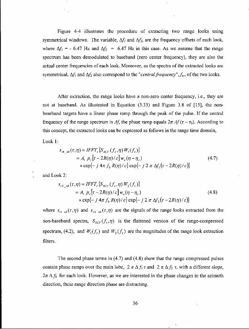
Figure 4-4 illustrates the procedure of extracting two range looks using

symmetrical windows. The .variable, Af and A/2, are the frequency offsets of each look,

where A/} = - 6.47 Hz and A/2 = 6.47 Hz in this case. As we assume that the range

spectrum has been demodulated to baseband (zero center frequency), they are also the

actual center frequencies of each look. Moreover, as the spectra of the extracted looks are

symmetrical, A/1 and A/2 also correspond to the "central frequency", fTC, of the two looks.

After extraction, the range looks have a non-zero center frequency, i.e., they are

not at baseband. As illustrated in Equation (3.33) and Figure 3.8 of [15], the non-

baseband targets have a linear phase ramp through the peak of the pulse. If the central

frequency of the range spectrum is Af the phase ramp equals 2n Af (r - ro). According to

this concept, the extracted looks can be expressed as follows in the range time domain,

Look 1:

srl _nb (T, rf) = IFFTr {SRCF (fr, 77) Wx (/r)}

= Axpr[r-2R(r1)lc]wa(r1-rlc) (4.7)

x exp{- j An f0 R{rj) I c] exp{- j 2 n Af (T - 2R(TJ) I c)}

and Look 2:

' , 2 _ * <J>V) = IFFTr {SRCF (fT,77) W2 (fT)}

= 4 pr[t-2R{i1)lc}wa(r1-rlc) (4.8)

x exp{- j An f0 R(rj) I c] exp{- j 2 n Af2 (r - 2^ (7 ) /c)}

where srl nb(T,Tj) and sr2 nb(r,r/) are the signals of the range looks extracted from the

non-baseband spectra, SRCF(fr,rj) is the flattened version of the range-compressed

spectrum, (4.2), and W^f) and W2(fr) are the magnitudes of the range look extraction

filters.

The second phase terms in (4.7) and (4.8) show that the range compressed pulses

contain phase ramps over the main lobe, 2 K Af x and 2K Af x, with a different slope,

2z Afk for each look. However, as we are interested in the phase changes in the azimuth

direction, these range direction phase are distracting.

36

4.2.2 Shifting to baseband

In order for the azimuth phases of the two looks to be easily compared, the range

center frequencies of the two looks can be moved to the same frequency. For conceptual

simplicity, the new centers will be moved to zero (baseband), where the phases over the

main lobe of the compressed pulses are flat [26].

This bandshifting is done after the range look extraction step. As the shift in the

frequency domain corresponds to a modulation in time domain, the signal of two

extracted looks after the spectrum shift can be expressed in the time domain as,

Look 1:

sri (r, 7) = IFFTr {SRCF (fT + Afx, 77) Wx (/r + Afx)}

= 4 pr[r-2tf(77)/CK(77 - 77c) (4.9) xexp{- j ATV (TO +Afx)R(rj)lc}

and Look 2:

sjT,T,) = IFFTr{S^(Sr+Af2,r!)W2lfT + Af2)}

= A]pr[T-2R(rj)/c]wa(rJ-rJc) (4.10)

x exp{- j 4TT (/„ + Af2 )R(rj)/c}

where sr] (r, 77) and sr2 (r, 77) are the signals of the range looks extracted from baseband

spectra. It can be seen that after shifting the spectra to baseband, the z dependence of the

phase is removed and the extracted looks are conditioned to generate the appropriate beat

signal.

Figure 4-5 illustrates the frequency response and the impulse response of the

baseband extracted looks in the single target simulation. It can be seen that the two

baseband looks have the same phase slope ramps in the frequency response, but the

phases at the central frequency (i.e., zero frequency) are different. In addition, the phases

at the central frequency correspond to the phase of the main lobe in the impulse response,

which verifies the theory discussed in Section 4.1.2 and 4.1.3.

37

T3

"c O ) ns

2000 r ' 0 0 ' < s n a v e * n e same magnitude spectrunj

1500 L a ' baseband

1000

500

0

300

200

100

0

-100

-200

Lookl: Phase at ce n-freq: -1:95 rads

400

<D 300 T3

H 200 E

K 100

0

*> 2 ra

oT o tn ra

2 lo Dks have the sam e ampliti ide enve ope

128 130 132 134 136

Phase

Look 1

of main lobe: -1.95 rads / -20 20 128 130 132 134 136

-20 0 20 Range frequency (MHz)

-5T 2

IK

v Look 2

Phase of main lobe: 2.55 rads \ 128 130 132 134 136

Range time (cells)

(a) Frequency response (b) Impulse response

Figure 4-5 Illustrating the phase relationship between frequency and time domain after shifting the extracted looks to baseband

4.2.3 Properties of the beat signal

After the shifting, the beat signal can be derived from the two baseband-extracted

looks, (4.9) and (4.10), by multiplying one look with the conjugate of the other:

hem 0", V) = sr' 7) sr2 (r, 77)

=|4 wa(rj -t]cf exp{-; 4 n AfrR(rf)lc)

38

where Afr = Af2 - A/, is the frequency difference of the two range looks.

It can be seen from (4.11) that the phase of the beat signal varies with azimuth

time because of the change of the slant range function, R(rj). If we expand R(rj) about the

central illuminated time, r\c, and ignore the small higher order components, the range

between target and radar can be given by:

1 V 2 cos2 6 R(rJ) = R(rJc) - ^sin^ i C (7-7 c ) + ~ r (?-7 c ) 2 (4.12)

where Vr is the effective radar velocity and 6 r,c is the beam squint angle measured in the

slant range plane.

In (4.12), R(rj) has a linear and quadratic components. The linear component gives

rise to a pure sine wave in the beat signal, whose frequency is given by:

2Afr dR(rj) = 2Afr Vr sm9rc = _

dr] c /„

where / = -2 Vr sin 0r c IA is the Doppler centroid frequency.

Jbeal — j „ _ _ ~ r J V \ H - l : > )

The quadratic component gives rise to a non-zero bandwidth in the beat signal.

Usually the bandwidth of the beat signal is quite small compared to the PRF. Hence, the

beat signal can be approximated by a single frequency with noise. The bandwidth of the

beat signal will be discussed in more detail in Section 5.1.

In summary, the beat signal has an average frequency proportional to the absolute

Doppler centroid frequency, which we are trying to estimate. The proportionality factor is

the fractional separation of the range looks, Afr I / „ . At this point, the requirement of the

symmetrical magnitude spectrum is recognized. If the looks are not symmetrical, the

average frequency calculated from the beat spectrum will not equal (4.12), and a different

look separation Afr must be "calibrated", as illustrated in Figure 4-2.

39

4.3 Cross Beating and the Use of RCMC

As described in the opening paragraph, as the existence of RCM in the received

data may limit the signal duration within one range cell and reduce the sensitivity of the

frequency estimation, there are some advantages to using RCM Correction (RCMC) in

the MLBF algorithm. In this section, we discuss two phenomena that reduce the purity of

the beat signal, and how range cell migration correction (RCMC) can be used to alleviate

them.

4.3.1 The effect of the cross beating

The MLBF concept outlined in Section 4.2 is based on a single target in each

range cell, which leads to the derivation of the beat signal, (4.13). However, in practice

there is inevitably more than one target in each range cell. This leads to a cross beating

effect that distorts the beat signal [13]. The cross beating arises when more than one

significant target is present in a range cell, and the Lookl of one target beats with Look 2

of other targets. The beating between different targets (cross-beating) gives rise to

spurious frequency components in the beat spectrum. Depending on the number, strength

and distribution of the extra targets, the cross-beating can distort the beat spectrum or add

noise to it.

In order to understand the effect of the cross beating, we first analyze the case of

two targets. Consider two targets P and Q, which are in the same range cell but separated

in azimuth, with beam center crossing times, r\p and r\Q. Then, the two range looks,

s^rj) and s2(n), can be expressed as [13],

Look 1:

)K(i7-7,)J 4/-,)*(7-7e)

(4.14)

40

and Look 2:

^ 2 ( V ) = SP2(T]) + SQ2(TJ)

(4.15)

where sn(rj), sP2(rj), and sQX(rj), sQ2(rj) are the range compressed signals of Look 1

In (4.16), the first term represents the beat signal generated by Target P alone, the

second term represents the beat signal generated by Target Q alone. These two auto-beat

terms provide correct beat frequency, as in the case of single target. However, the third

and fourth terms represent the signals generated by a target in one look beating with

another target in the other look, a phenomenon referred to as cross beating.

The cross beating leads to extra frequencies in the beat signal spectrum. The third

term of (4.16) can be expanded as:

and Look 2 for Targets P and Q individually, Ap and AQ are the amplitude of the targets

after range compression and look extraction.

Then, the beat signal in this case becomes:

Sbeal

(Jl) = s\ (7) -*2 07)

= sP '(7)• sP2(7) + sQ'(n)• sQ2(rj)

+ sP* (7) ' sQ2 (7) + (7) • sP2 (7)

(4.16)

sP'(ri)-sQ2(Tj)

Ap*AQwa(n--nc--nP)wa(r]-?]c-nQ) (4.17)

exp jy [(/0 + A/, )R(T1-T1p)- (f0 + A/ 2 )R(TJ - rjQ)]

Using the expansion for R(rj) of (4.12), the frequency of this cross term is:

41

J P'Q

2 d[(f0 + A/, )R(rj - 1 7 , )-(/"<> + Af2 )R(r1 - nQ )]| c drj

2{Af2 -Af)Vr s in^ c 2Vr

2 cos2 6rJ, 1=1c

• cR(r]c) (4.18)

= fbeal

where fbea, is the single-target beat frequency defined in (4.13), Ka is the Doppler FM

rate of the signal, and Arj - t]Q - rjp is the separation of the two targets in azimuth time.

Similarly, the cross frequency of the forth term of (4.16) can be expressed as:

fro.^fbea.-K^Arj (4.19)

The cross beating leads to these extra frequencies in the beat signal spectrum.

Equations (4.18) and (4.19) show that the offset, ±KaArj, of the cross-beating

frequencies from the expected beat frequency depends on the Doppler FM rate and the

target separation, but does not depend on the look separation, Af2 - A/,.

The amplitude of the cross-beating signals is usually less than the main beat

signal, as one target is often smaller than the other target and because the duration of the

overlap of the two targets is less than the exposure time of one target. Thus, the beat

spectrum is not distorted much if \Ap\ » \AQ\ and/or if the targets are well separated in

azimuth. However, the effect of the cross beating on the spectrum becomes noticeable

when AQ becomes close to Ap in magnitude and there is substantial overlap between the

targets.

42

(a) The beat spectrum of a single target

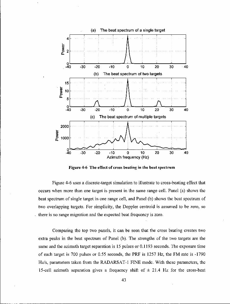
Figure 4-6 uses a discrete-target simulation to illustrate to cross-beating effect that

occurs when more than one target is present in the same range cell. Panel (a) shows the

beat spectrum of single target in one range cell, and Panel (b) shows the beat spectrum of

two overlapping targets. For simplicity, the Doppler centroid is assumed to be zero, so

there is no range migration and the expected beat frequency is zero.

Comparing the top two panels, it can be seen that the cross beating creates two

extra peaks in the beat spectrum of Panel (b). The strengths of the two targets are the

same and the azimuth target separation is 15 pulses or 0.1193 seconds. The exposure time

of each target is 700 pulses or 0.55 seconds, the PRF is 1257 Hz, the FM rate is -1790

Hz/s, parameters taken from the RADARSAT-1 FINE mode. With these parameters, the

15-cell azimuth separation gives a frequency shift of ± 21.4 Hz for the cross-beat

43

components. Therefore, the frequency shift of the cross-beating components observed in

Panel (b) agrees with the offset frequencies of (4.18) and (4.19).

Panel (c) shows the extra distortion that occurs in the beat spectrum when there

are many targets in the same range cell. In this simulation, there are 20 targets with a

random separation in azimuth between 1 and 3 pulses. The target amplitudes are equal at

one unit, and Gaussian noise is added with an RMS value of unity. The cross-beating

components in the same range cell add coherently, which can result in spurious peaks and

nulls in the beat spectrum.

In general, the cross-beating increases with the density of the targets. When the

density is too high, the beat frequency may not be detected within the ambiguity error

limits. That is why it is more difficult to estimate the beat frequency when there are many

targets with similar magnitude, as in homogeneous, low contrast scenes.

4.3.2 The effect of RCM

A significant amount of range cell migration (RCM) is often present in satellite

SAR data. With the existence of RCM, the signal trajectory has a slope over azimuth and

the signal energy can be spread over several range cells during the exposure time. In this

case, each target is fragmented in each range cell. As a consequence, the fragmented

exposure time of the target in each rang cell leads to a wider peak and less resolution in

the beat signal spectrum. Moreover, the partial exposures that exist with RCM create a

higher density of targets in each range cell, resulting in more cross beating.

The effect of RCM is illustrated in Figure 4-7, which compares the trajectories of

two targets that have a small displacement in range and azimuth. Panel (a) shows the

locus of target energy in the range compressed data with no RCM, as in the case where

the beam is steered to zero Doppler. When the Doppler centroid is well away from zero,

significant RCM can be present, as shown in Panel (b).

44

Range cells beating Range cells beating

(a) With No R C M (b) With significant R C M

Figure 4-7 Distribution of the energy of two targets in range-compressed data

Figure 4-7 illustrates the effect of RCM, which compares the trajectories of two

targets that have a small displacement in range and azimuth. Panel (a) shows the locus of

target energy in the range compressed data with RCM, while Panel (b) shows the locus

without RCM. It also can be seen that with RCM the target exposure time in each cell,

Tajeat = 1/5 Ta, is only one fifth of that without RCM, Ta_beat = Ta. In addition, the

partial exposures that exist with RCM create a higher density of targets in each range cell,

resulting in more cross beating.

Two effects are noticed in Figure 4-7. First, the exposure time of each target is

reduced by the RCM, when observed within a single range cell. In this example, the

exposure time within a range cell has been reduced to Ta I 5 by the 5-cell RCM, where Ta

is the full exposure time of a target. As the beat signal takes place within one range cell,

the reduced exposure time means that the resolution of the beat signal is broadened.

Second, while there is only one target in each range cell when there is no RCM, the RCM

has created two targets in each cell. This creates the cross-beating effect discussed in

Section 4.3.1, as long as the partial exposures overlap. Both of these effects reduce the

45

sensitivity of the beat frequency estimation. The cross-beating effect tends to get larger

when a high density of targets is present, although the target overlap is reduced when the

exposure within a cell is smaller.

Figure 4-8 illustrates the effect of the RCM on the beat spectra using a discrete-

target simulation. RADARS AT-1 FINE parameters are used, with a PRF of 1257 Hz and

an exposure time of 700 pulses. Three cases of RCM are shown. In the first row, the

Doppler centroid is set to zero, so there is no linear RCM, and only a small amount of

quadratic RCM (about half a cell). In the second row, the Doppler centroid is set to 4.7

PRFs, giving the target(s) an RCM of 20 cells. In the third row, the Doppler centroid is

set to 9.4 PRFs, giving the target(s) an RCM of 40 cells.

20

No RCM I 10 Q -

Single target Two targets Multiple targets 40

20

It t A :

-20 0 20 40 60 80 -20 0 20 40 60 80 -20 0 20 40 60 80

| 4

RCM: 20 cells § Q. 2

10

5

40

20

-20 0 20 40 60 80 -20 0 20 40 60 80 -20 0 20 40 60 80

a> 4 RCM: 40 cells §

o- 2

40

20

0 -20 0 20 40 60 80 -20 0 20 40 60 80 -20 0 20 40 60 80 Azimuth frequency (Hz) Azimuth frequency (Hz) Azimuth frequency (Hz)

Figure 4-8 Illustrating the effects of R C M on the beat signal resolution - single, double and multiple targets case

46

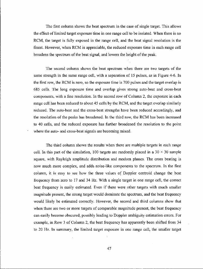
The first column shows the beat spectrum in the case of single target. This allows

the effect of limited target exposure time in one range cell to be isolated. When there is no

RCM, the target is fully exposed in the range cell, and the beat signal resolution is the

finest. However, when RCM is appreciable, the reduced exposure time in each range cell

broadens the spectrum of the beat signal, and lowers the height of the peak.

The second column shows the beat spectrum when there are two targets of the

same strength in the same range cell, with a separation of 15 pulses, as in Figure 4-6. In

the first row, the RCM is zero, so the exposure time is 700 pulses and the target overlap is

685 cells. The long exposure time and overlap gives strong auto-beat and cross-beat

components, with a fine resolution. In the second row of Column 2, the exposure in each

range cell has been reduced to about 45 cells by the RCM, and the target overlap similarly

reduced. The auto-beat and the cross-beat strengths have been reduced accordingly, and

the resolution of the peaks has broadened. In the third row, the RCM has been increased

to 40 cells, and the reduced exposure has further broadened the resolution to the point

where the auto- and cross-beat signals are becoming mixed.

The third column shows the results when there are multiple targets in each range

cell. In this part of the simulation, 100 targets are randomly placed in a 30 x 30 sample

square, with Rayleigh amplitude distribution and random phases. The cross beating is

now much more complex, and adds noise-like components to the spectrum. In the first

column, it is easy to see how the three values of Doppler centroid change the beat

frequency from zero to 17 and 34 Hz. With a single target in one range cell, the correct

beat frequency is easily estimated. Even if there were other targets with much smaller

magnitude present, the strong target would dominate the spectrum, and the beat frequency

would likely be estimated correctly. However, the second and third columns show that

when there are two or more targets of comparable magnitude present, the beat frequency

can easily become obscured, possibly leading to Doppler ambiguity estimation errors. For

example, in Row 3 of Column 2, the beat frequency has apparently been shifted from 34

to 20 Hz. In summary, the limited target exposure in one range cell, the smaller target

47

overlap and the cross-beating of multiple targets tend to increase the error in the

estimation of the beat frequency as the RCM increases

4.3.3 Benefit of applying RCMC

In this section, we discuss the benefits of applying RCM Correction (RCMC)

before the beat frequency is estimated. When RCMC is applied with the correct

ambiguity number, each target is confined to one range cell, and the beat signal arising

from a target beating with itself (auto-beating) has the finest possible resolution.

However, there is another effect of RCMC, which may help or hinder the beat

signal frequency estimation, depending on the distribution and strength of targets. RCMC

may bring other targets into the same range cell, with a full exposure. The overlap with

the existing target may be larger, giving rise to a stronger, sharper, cross-beat component.

Figure 4-9 illustrates how RCMC can help to improve the beat frequency estimation. In

the simulation, 100 targets are used, randomly placed within a 30 x 30 sample grid. Their

amplitudes have a Rayleigh distribution, and their phases are random. Panel (a) shows the

beat spectrum before RCMC, while Panel (b) shows the spectrum after RCMC. The beat

spectrum has been averaged incoherently across range cells.

Due to the effect of the RCM and the cross beating, the spectrum before RCMC is

wide and noisy in Panel (a). But after RCMC in Panel (b), a much cleaner, narrower

spectrum results from increasing the exposure time in each range cell, and reducing the

cross beating. In this example, there is an average of three targets in each range cell. The

narrow peak increases the accuracy of the MLBF algorithm by improving the estimation

of the beat frequency.

48

(a) Multiple targets - before RCMC

§ 0.5

„ . .- 1 . . 1

f =15 96Hz —>i

_

beat •

i V

i i 1

1

§ 0.5 0-

1

§ 0.5

0

-30 -20 -10 0 10 20 30 40 50 60

(b) After applying RCMC after look extraction I I

f ,=19.64Hz-J beat 71

_

r i i \ r

-30 -20 -10 0 10 20 30 40 50 60

(c) After applying RCMC before look extraction

_ I I I

f , =O.O0Hz - J beat fil

_

0 -30 -20 -10 0 10 20 30 40 50 60

Azimuth frequency (Hz)

Figure 4-9 Illustrating the effects of RCMC on the beat signal resolution

4.3.4 Examples with real data

In our study, the RADARSAT-1 fine mode scene of Vancouver is selected to

illustrate the properties of Doppler estimators. The processed image of the whole scene is

shown in Figure 4-10. There is water, farmland, city and mountains in the scene [15].

49

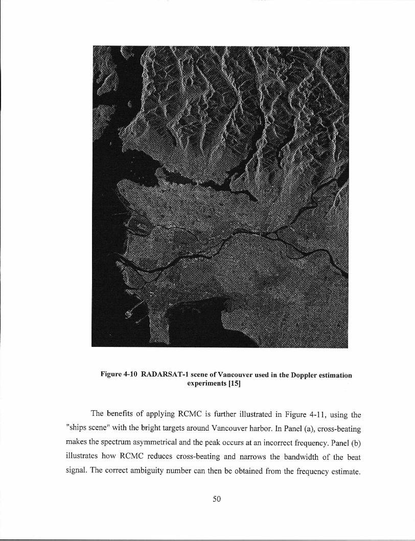
Figure 4-10 R A D A R S A T - 1 scene of Vancouver used in the Doppler estimation experiments [15]

The benefits of applying RCMC is further illustrated in Figure 4 - 1 1 , using the

"ships scene" with the bright targets around Vancouver harbor. In Panel (a), cross-beating

makes the spectrum asymmetrical and the peak occurs at an incorrect frequency. Panel (b)

illustrates how RCMC reduces cross-beating and narrows the bandwidth of the beat

signal. The correct ambiguity number can then be obtained from the frequency estimate.

50

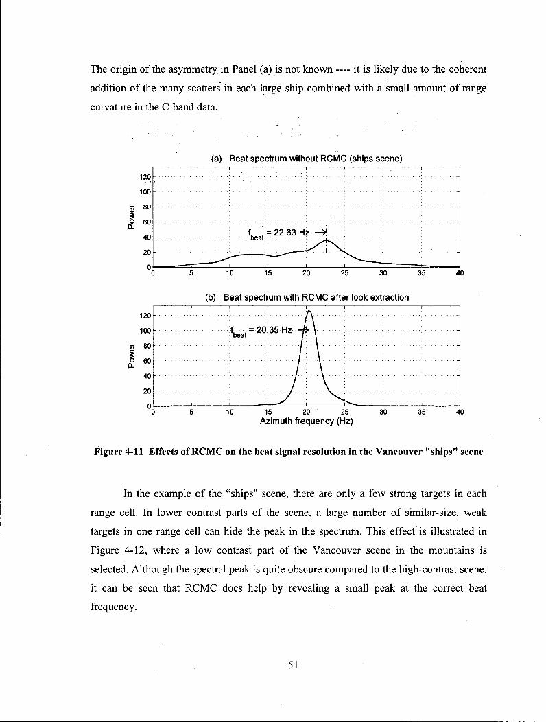
The origin of the asymmetry in Panel (a) is not known — it is likely due to the coherent

addition of the many scatters in each large ship combined with a small amount of range

curvature in the C-band data.

120

100 8 0

O 60 Q.

40

20

0

(a) Beat spectrum without RCMC (ships scene) i i i

f =22.63 H z -»i beat :

i \ i • i i

i \ r —*

10 15 20 25 30 35 40

120

100

fc 80

O 60 D.

40

20

0

(b) Beat spectrum with RCMC after look extraction

f - on OK u-» _bJ \ : b e a < : /

10 15 20 25

Azimuth frequency (Hz) 30 35 40

Figure 4-11 Effects of RCMC on the beat signal resolution in the Vancouver "ships" scene

In the example of the "ships" scene, there are only a few strong targets in each

range cell. In lower contrast parts of the scene, a large number of similar-size, weak

targets in one range cell can hide the peak in the spectrum. This effect is illustrated in

Figure 4-12, where a low contrast part of the Vancouver scene in the mountains is

selected. Although the spectral peak is quite obscure compared to the high-contrast scene,

it can be seen that RCMC does help by revealing a small peak at the correct beat

frequency.

51

Figure 4-12 Effects of R C M C on the beat signal resolution in the Vancouver "mountains"

scene

4.3.5 Why RCMC must be applied after look extraction

As illustrated Section 4.1.2, it is the variation along azimuth of the slope of the

phase in the range spectrum that makes the MLBF algorithm work. Therefore, if RCMC

is to be applied in the MLBF algorithm, one must be careful not to destroy this phase

variation.

Case I: RCMC before look extraction

If we apply RCMC before range look extraction, the RCMC changes the target

range from R(rf) to *o in all range lines in (4.2), where RQ is the reference slant range for

that target. This has the effect of removing the phase ramp along azimuth time after the

52

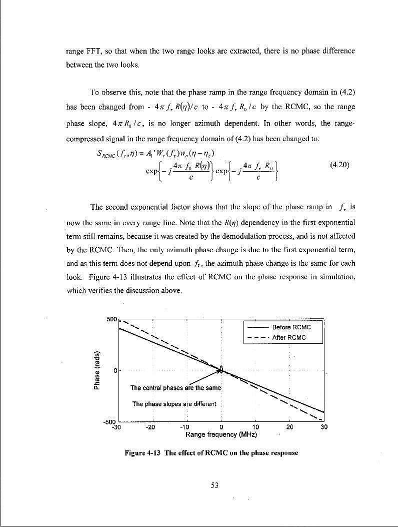
range FFT, so that when the two range looks are extracted, there is no phase difference

between the two looks.

To observe this, note that the phase ramp in the range frequency domain in (4.2)

has been changed from - 4K fT R(rj)/c to - 4K fr R0 fc by the RCMC, so the range

phase slope, 4KR0/C, is no longer azimuth dependent. In other words, the range-

compressed signal in the range frequency domain of (4.2) has been changed to:

The second exponential factor shows that the slope of the phase ramp in fT is

now the same in every range line. Note that the R(rf) dependency in the first exponential

term still remains, because it was created by the demodulation process, and is not affected

by the RCMC. Then, the only azimuth phase change is due to the first exponential term,

and as this term does not depend upon fr, the azimuth phase change is the same for each

look. Figure 4-13 illustrates the effect of RCMC on the phase response in simulation,

which verifies the discussion above.

Figure 4-13 The effect of R C M C on the phase response

53

Correspondingly, the two range looks extracted from the signal after RCMC can

be expressed as,

Lookl:

srl'(r,rj) = Al pr[r-2RJc\wa{r1-rlc)

x exp{- j An f0 R(JJ) I c] exp{; A n Afx RJc]

And Look 2:

sr2'(r,r/) = A] pr[T-2RQ/c]wa(rj-Tjc) (422)

xexp{- j An./„ R(TJ)Ic]exp{- j An Af2RJc}

As a result, in the case of applying the RCMC before look extraction, the beat

signal can be expressed as:

sbea,f(j^) = s/{r,T])sr2\T,r])

= \A w

a (7-7 e ) | 2 exp{-;4^ Afr RJc)

As the phase of the beat signal is a constant in azimuth (compare (4.23) with

(4.11)), the beat signal has zero frequency, and the information used to obtain a Doppler

estimate has been lost, as follows:

/ ^ ' = ^ ^ = 0 (4.24) c drj

Figure 4-14 illustrates the simulation results in this case. It can be seen that the

phases of the two looks have the same changing pattern and hence their difference is

constant. As a consequence, the beat frequency obtained from the two looks is zero, and

thus cannot be used to obtain a Doppler estimate.

54

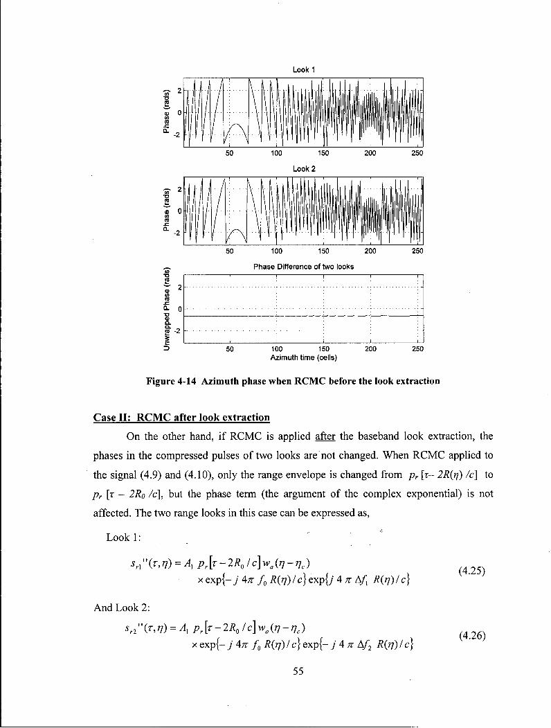
Look 1

Azimuth t ime (cells)

Figure 4-14 Azimuth phase when R G M C before the look extraction

Case I I : RCMC after look extraction

On the other hand, if RCMC is applied after the baseband look extraction, the

phases in the compressed pulses of two looks are not changed. When RCMC applied to

the signal (4.9) and (4.10), only the range envelope is changed from pr [x- 2R(rf) /c] to

pr [T - 2Ro /c], but the phase term (the argument of the complex exponential) is not

affected. The two range looks in this case can be expressed as,

Look 1:

sH''(T,TJ) = A, pr[T-2R01c] wa(TJ-T]C)

x exp{- j An /„ R(ij) I c] exp{/ 4 n A/, R(rj) I c)

And Look 2:

sr2''(T,77) = A, pr[T - 2R01c] wa(TJ-TJC)

xexp{- j An /„ R(TJ)Ic)exp{- j An Af2 R(n)Ic]

(4.25)

(4.26)

55

Consequently, the azimuth phase difference of the two looks still maintains the

correct dependence on the range migration. Figure 4-15 shows azimuth phase plots when

RCMC is applied after the look extraction. Comparing to Figure 4-14, the phase

difference of two looks is not constant, but changing with azimuth time. Moreover, it can

be seen that the phase difference is almost a linear function of azimuth time, and the slope

of the linear phase gives the value of the beat frequency. As a result, the correct Doppler

estimate can be obtained from this phase variation.

Look 1

Azimuth time (cells)

Figure 4-15 Azimuth phase when R C M C after the look extraction

These effects are illustrated in the Panels (b) and (c) of Figure 4-9. In Panel (b),

RCMC is applied after range look extraction, and the benefits of RCMC described in

Section 4.3.3 are obtained. In Panel (c), however, RCMC has been applied before range

56

look extraction, the beat frequency has been shifted to zero, and the distinctive beat

frequency, has been lost.

In conclusion, applying RCMC after look extraction gives the same beat

frequency as without RCMC, but applying RCMC before the look extraction shifts the

beat frequency to zero. Therefore, the RCMC should be applied after the baseband look

extraction in order to preserve the correct beat frequency [26].

4.4 Iterative Procedure Using RCMC

The existing MLBF algorithm is not as reliable as it could be, due to the coarse

resolution of the beat frequency and the occurrences of the cross-beating between

multiple targets in one range cell. In this section, the implementation scheme of the

method using RCMC is discussed and the experimental results on real satellite SAR data

show that this method has a better performance than the existing MLBF algorithm.

4.4.1 The iterative procedure

RCMC can only be applied correctly if the Doppler ambiguity number is known,

which is not available until after the current estimation procedure is completed. Hence, in

order to take advantage of the RCMC routine in the MLBF algorithm, an iterative

procedure is proposed — see the flowchart in Figure 4-16.

57

Range compressed data

Range FFT

Flatten the range spectrum

Extract two range looks

Shift the looks to baseband

Estimate baseband Doppler centroid

Range IFFT

Generate the beat signal

Estimate the beat frequency

Calculate the absolute Doppler Centroid

Resolve the Doppler ambiguity number

Generate look extraction windows

Apply RCMC to the current looks, using

the current ambiguity estiamte

Yes

Is it the first Iteration; or the current""

estimate is different from the previous one?

No

Output ihe final Doppler ambiguity cstinuiv.'

Figure 4-16 Flowchart of the proposed R C M C / M L B F algorithm

In the first iteration, since we don't yet know the absolute Doppler centroid, the

conventional MLBF algorithm can be implemented without RCMC to obtain the initial

58

estimate. In some cases, an initial estimate of the Doppler centroid from geometry can be

used in the first iteration. In subsequent iterations, RCMC can be applied using the

current Doppler ambiguity estimate. As the RCMC is refined, the bandwidth of the beat

signal is reduced, and lower bandwidth will benefit the ILP frequency estimator. The

iterations continue until the Doppler ambiguity settles down to a stable value — we have

found that usually only two iterations are required with real data (see Section 4.4.2). Note

that in this method, as in other ambiguity resolvers, the baseband Doppler estimates are

obtained first and unwrapped so that a single Doppler ambiguity number applies over the

whole scene.

As the iterative algorithm requires applying the RCMC and the MLBF algorithm

more than once, the computation time is a little more than the standard MLBF algorithm.

As the RCMC is applied after range look extraction, the look extraction is only applied

once as the RCMC is changed. We have found that the extra computation load is

acceptable, and the iterative MLBF computation only occupies a small portion of the

whole SAR processing time.

4.4.2 Experimental results

In Section 4.3.4, the Vancouver "ships" and "mountains" scenes give two

examples of how the iterative RCMC method can improve the sensitivity of the MLBF

algorithm. In order to test its performance on different kinds of terrain in satellite SAR

data, we apply them to real SAR data of RADARS AT-1 find mode Vancouver scene, as

shown in Figure 4-10. In order to take advantage of spatial averaging and avoid bad

estimates from areas with very weak backscatter, we make use of the concept of "spatial

diversity" [19]. In this approach, the whole scene is divided into blocks, the estimators are

applied and specific quality measurements are calculated for each block to exclude areas

of the scene that are likely to lead to incorrect Doppler estimates. In this experiment, we

divide the Vancouver data set into 12 range x 19 azimuth blocks, with each of the 228

blocks having 655 range cells and 1024 range lines. The block borders are outlined in the

"range-compressed image" of Figure 4-17.

59

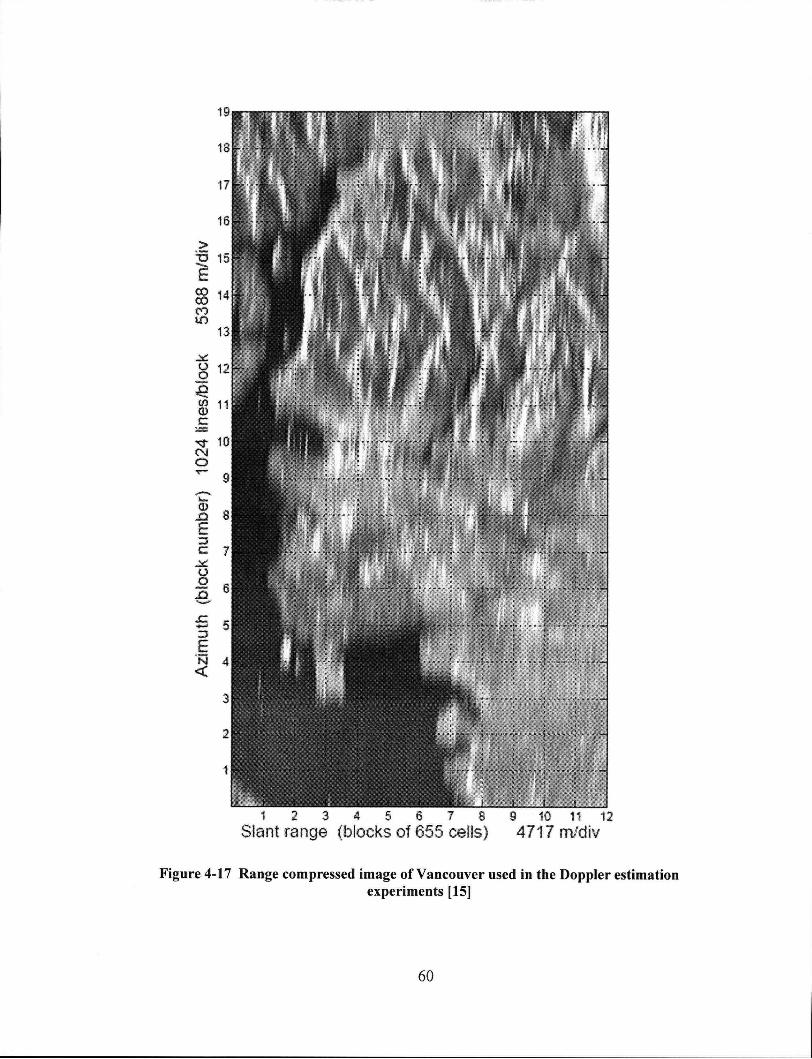
1 2 3 4 5 6 7 8 9 10 11 12 Slant range (blocks of 655 cells) 4717 m/div

Figure 4-17 Range compressed image of Vancouver used in the Doppler estimation experiments [15]

60

Both the standard MLBF algorithm and the iterative MLBF algorithm using

RCMC are implemented for each block. In this experiment, we use the frequency

estimator based on the FFTs to estimate the beat frequency [13]. After processing all the

blocks, the blocks with the possible bad estimates are removed using quality criteria. In

order to compare the performances of all methods, the same quality criterion (the SNR of

the range-compressed data larger than -1 dB) is applied in each case, so that the same

blocks are removed. Then, a single Doppler ambiguity number is obtained for the whole

scene using a "majority vote" or an average operation.

The iterative RCMC method shows an even better improvement. It has the highest

success rate of all the estimators. Because the beat spectrum is cleaner after RCMC, the

choice of frequency estimator is not so critical, and the simple FFT estimator works well.

200

Ambiguity Number

Figure 4-18 Histogram of the M L B F estimates of each block with and without R C M C

61

Table 4-1 Doppler Ambiguity estimates using Standard MLBF and the proposed method

Doppler Ambiguity estimators Mean (PRFs)

St. Dev. (PRFs)

Success rate (%)

Standard MLBF -5.74 1.09 62

Iterative MLBF using the RCMC -5.92 0.73 92

The histogram and the comparison table show that the iterative MLBF using

RCMC has a much better performance than the existing standard MLBF. The Standard

deviation is reduced by about 30%, and the success rate increases considerably to 92%. In

this experiment, most of the blocks that are taken as the good estimates only need two

iterations. Only 2% blocks with good estimates need three iterations.

4.5 Summary

The MLBF algorithm is the one of the most reliable methods for Doppler

ambiguity resolution. By examining the phase of the frequency-domain signal, we found

that the azimuth phase variation caused by range migration plays an important role in the

generation of the beat signal. We also presented the importance of having symmetrical

range looks.

Then, we presented the method of applying RCMC to improve the sensitivity of

the MLBF algorithm. The cross beating caused by multiple targets in a range cell

introduces spurious signals into the spectrum of the beat signal. The presence of RCM

reduces the exposure time in one range cell and thereby broadens the resolution of the

beat signal. Then, we have shown how RCMC can alleviate these effects by increasing

the resolution of the beat signal, and possibly reducing the cross beating. The analysis

also shows that RCMC must be applied after the range look extraction, and that an

iterative scheme must be used because the correct ambiguity is needed to perform RCMC

62

properly. Finally, experiments with RADARSAT-1 data are used to illustrate the

improved estimation accuracy of the modified algorithm.

63

Chapter 5

Improved Beat Frequency

Estimation in the MLBF algorithm

Among the Doppler ambiguity resolvers, the Multi-look Beat frequency (MLBF)

algorithm proves to have good performance, especially in high contrast areas. It also

avoids estimating the offset frequency, which is required in the WDA and MLCC

algorithms. However, the existing MLBF algorithm has some problems. As it uses FFT

operations to measure the central frequency of the beat signal by finding the maximum

coefficient, it leads to quantization errors as only the energy at discrete frequencies is

evaluated. In this method, the limited exposure in each range cell also reduces resolution

of the spectrum. In addition, the algorithm using FFTs requires a zero-padding procedure

when applied to burst mode data, such as ScanSAR data [13]. Therefore, more efficient

and accurate methods are required to improve the performance of the MLBF algorithm

In this chapter, several frequency estimators are introduced to improve the beat

frequency estimation in the MLBF algorithm. First, the center of gravity is used to

measure the beat frequency from the beat signal spectrum. Then five established

frequency estimators based on phase increments are applied to measure beat frequency

from the phase information.

5.1 The Principle of the Beat Signal

As described in Chapter 3 and Chapter 4, the MLBF algorithm is based on the

fact that the Doppler Centroid frequency can be derived from the azimuth phase

difference between two looks that are extracted from the range spectrum. By multiplying

64

the signal of one look with the conjugate of the other look, a beat signal results, which

can be expressed as [15]:

sbea,(j^) = sr,\r,ri)srl(T,T1)

=\A ™a(n-Vcf e xp{-j 4 K R{rj)ic}

where Afr - Hf2 - A/y. A/y and A/2 are the central frequencies of the two range looks

separately, assuming the two looks have symmetrical magnitude spectra.

To examine how the beat signal varies with azimuth time, we expand the slant

range function R(rf) about the central illumined time nc. If the small higher order

components are ignored, the range between target and radar can be given by:

\V2cos29rc

R(rj) = R(r1c)-Vr sin0 ( 7 - 7 c ) + - r'c (rj-n,)2 (5.2) 2 R(TJC)

where 9rc is the beam squint angle measured in the slant range plane

As the linear component, - Vr sin Orc(n-nc) , has a much larger value than the

quadratic component, — ^ ° ° S ^ r , c (77 -nc), the beat signal expressed by (5.2) mainly 2 R(TJC)

contains a single frequency with a narrow bandwidth.

According to the phase history of (5.1), Figure 5-1 shows the Azimuth

frequency/time history of the beat signal. It can be seen that the beat signal has an average

(central) frequency and a bandwidth.

65

Azimuth frequency

PRF

ft beat

BWhe

Azimuth Time rj

Figure 5-1 The frequency spread-out of the beat signal along azimuth

The central frequency of the beat signal, feat, can be derived from the phase of

(5.1) and the linear component of (5.2), and is given by:

2Afr dRjrj) = 2Af Vr sin0rc = A / r

J beat j _ y J nc c dr] c

where fnc is the Doppler Centroid frequency and /

fo

2 Vr s\ndr

(5.3)

Similarly, the bandwidth of the beat signal, BWbeat, can be derived from the phase

of (5.1) and the quadratic component of (5.2), which is expressed as:

EW Wrd2R(T})_ ¥ r Vr" C O S 2 0„ be°'~ c dr]2 ~ cR(r]c) ( 5 4 )

= -^tL BW r '-'"azimuth

JO

where BWazimulh is the azimuth bandwidth of the received signal and V2cos26rc BW = - —

azimuth i n / \

66

Both the center frequency, fbeat, and the bandwidth, BWbeat, of the beat signal are

quite small compared to the system PRF. Taking the RADARSAT-1 Vancouver scene

data as an example, where f„c ~ -5900Hz, fbeat is about 21 Hz, the predicted BWbeal is

about 2.5 Hz, while the PRF is 1275 Hz, as shown in Figure 5-1. The small value of fbeat

compared to the PRF avoids unwrapping and makes this algorithm suitable for Doppler

ambiguity estimation. (The ambiguity error limits are +/- 3.5 Hz in this case.) The narrow

bandwidth, BWbeat, justifies that the beat signal can be approximated by a single

frequency with noise.

As the beat frequency is proportional to the absolute Doppler centroid in (5.3),

the absolute Doppler centroid frequency can be estimated from the measurement of the

beat frequency, which can be expressed as:

' .: fnc ~, ~ fbeat (5-5)

The above analysis is based on the existence of a single target in each range cell

without noise. However, in implementation noises are usually inevitable. In addition,

when there is more than one target, cross beating exists, which lowers the SNR of the beat

signal and makes it harder to estimate the beat frequency accurately [15].

5.2 Single Frequency Estimation

As discussed in Section 5.1, the beat signal can be approximated to a single

frequency signal with noise. Therefore, single frequency estimators can be applied to the

estimation of the beat frequency. In this section, the model for single frequency

estimation is established and analyzed. Then, the survey results give several single

frequency estimators and each estimator is described separately.

67

5.2.1 Introduction

The problem of estimating the frequency of a complex exponential in additive

white noise is a fundamental and well-studied problem in estimation theory. In particular,

consider the Appoint received data to consist of a single complex sinusoid in complex

white Gaussian noise, which has the form of:

x(n) - A exp{j(con + q>)} + z(n), (5.6)

n = 0, 1, 2, N-l

where co,- n < co< n, is the frequency in radians/sample, and A and <p, -n <<p <n

are unknown constants. The noise z is a zero-mean complex white Gaussian process with:

z(ri) - zr (n) + jzt (n). Its components zr (n) and z, (ri) are real, uncorrected, zero-mean

Gaussian random variables with variance cr212 (a2 is the variance of z(n) from the

calculation of £[(z («) - E (z(n)) ) (z (n) - E (z(n)) )*]. )

According to estimation theory, the ultimate accuracy bound for frequency

estimation is derived from the Cramer-Rao inequality, which is called the Cramer-Rao

Bound. The Cramer-Rao Bound can be calculated as [27]:

CRB = 6 , =— (5.7 SNRN(N2-l) A ^ N { N 2 _ V )

(7

where SNR is the Signal to Noise Ratio, and Af is the length of the signal array.

As illustrated in Figure 5-2, our survey results show that the frequency estimators

can be classified into two categories: algorithms based on FFTs and algorithms based on

phase increments. In the following sections, we will be discussing seven frequency

estimators. The methods based on FFTs include measuring the frequency of the

maximum FFT coefficient and measuring the Center of Gravity. The methods based on

phase increments include Kay's estimator, ACCC estimator, FCFB estimator, HLC

estimator and ILP estimator. The contents and the organization of the following

subsections are shown in Figure 5-2.

68

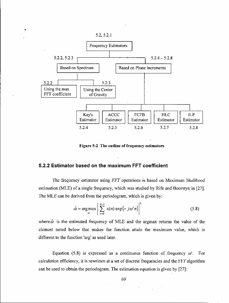
5.2, 5.2.1

Frequency Estimators

5.2.2, 5.2.3

Based on Spectrum

5.2.4-5.2.8

Based on Phase increments

5.2.2 Using the max FFT coefficient

5.2.3 Using the Center

of Gravity

Kay's Estimator

5.2.4

ACCC Estimator

5.2.5

FCFB Estimator

5.2.6

HLC Estimator

5.2.7

ILP Estimator

5.2.8

Figure 5-2 The outline of frequency estimators

5.2.2 Estimator based on the maximum FFT coefficient

The frequency estimator using FFT operations is based on Maximum likelihood

estimation (MLE) of a single frequency, which was studied by Rife and Boorstyn in [27].

The MLE can be derived from the periodogram, which is given by:

co = arg max A M

£ x(n)exp{-jco'n} n=0

(5.8)

whereby is the estimated frequency of MLE and the argmax returns the value of the

element noted below that makes the function attain the maximum value, which is

different to the function 'arg' as used later.

Equation (5.8) is expressed as a continuous function of frequency co'. For

calculation efficiency, it is rewritten at a set of discrete frequencies and the FFT algorithm

can be used to obtain the periodogram. The estimation equation is given by [27]:

69

2n co = arg max

NFFT OZm<NFFT-\

where Nfpr is the FFT length.

FFT

x(ri) exp{- j {InmnlNFFT)} n=0

(5.9)

It is straight-forward from equation (5.9) that the frequency can be estimated by

finding the discrete frequency that corresponds to the maximum FFT coefficient. The

existing MLBF algorithm uses such method in the beat frequency estimation. However,

this method leads to quantization error because it only evaluates the energy at discrete

frequencies. In this case, the maximum quantization error is given by:

4/1 = A V r

FFT-scale

fo 1 PRF Af 2 NFFT

(5.10)

In the implementation of RADARSAT-1 dataset, if we apply a 1024-point FFT

and separate the two range looks by about half of the range spectrum bandwidth, the

maximum quantization error is about 100 Hz. Since the existence of the quantization error

restricts the accuracy of the estimator even at high SNR, more accurate frequency

estimators are required to improve the beat frequency estimation.

5.2.3 Estimator based on the "center of gravity"

Since the frequency of the signal corresponds to the peak center of the signal

spectrum, we can measure the frequency by finding the "center of gravity" in the

spectrum of the beat signal in order to reduce the effects of the quantization errors and

other addictive errors [29]. Similar to Section 5.2.2, we use FFTs to obtain the spectrum

of the signal. Then, the single frequency can be estimated by this method using:

I>, FS, v = —N (5-11)

ZZFS, ;=1

70

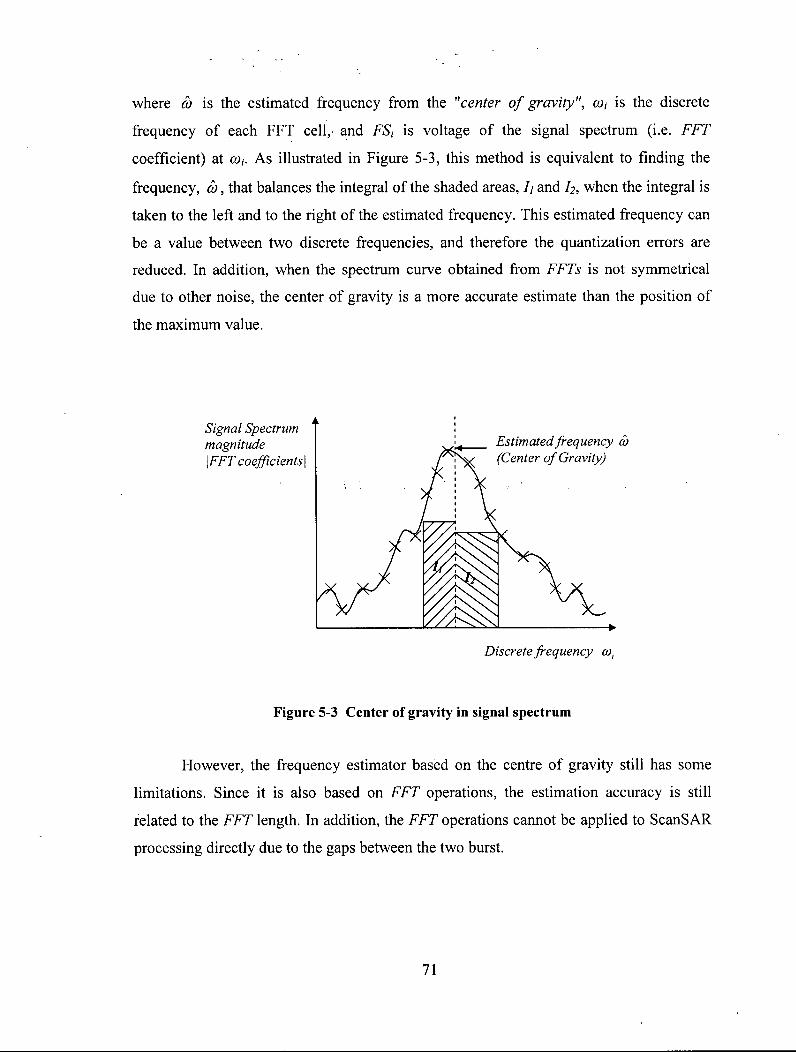
where co is the estimated frequency from the "center of gravity", (Oj is the discrete

frequency of each FFT cell, and FSt is voltage of the signal spectrum (i.e. FFT

coefficient) at co,-. As illustrated in Figure 5-3, this method is equivalent to finding the

frequency, co, that balances the integral of the shaded areas, /; and h, when the integral is

taken to the left and to the right of the estimated frequency. This estimated frequency can

be a value between two discrete frequencies, and therefore the quantization errors are

reduced. In addition, when the spectrum curve obtained from FFTs is not symmetrical

due to other noise, the center of gravity is a more accurate estimate than the position of

the maximum value.

Discrete frequency a>i

Figure 5-3 Center of gravity in signal spectrum

However, the frequency estimator based on the centre of gravity still has some

limitations. Since it is also based on FFT operations, the estimation accuracy is still

related to the FFT length. In addition, the FFT operations cannot be applied to ScanSAR

processing directly due to the gaps between the two burst.

71

5.2.4 Kay's estimator

The frequency estimators based on phase increments can avoid the problems and

limitations of the estimators based on the FFT operations. Kay's estimator (proposed by

Steven Kay in 1989 [30] ) is the basic single frequency estimator that uses phase

increments instead of the periodogram to estimate the signal frequency. If we assume that

the SNR, which is A21 cr2, is large, the data model of (5.6) can be rewritten by replacing

additive noise by phase noise, which is given by:

x(n) w A exp(y (an + cp + u(n) ) (5.12)

n = 0,1, 2,---,N-l

where u(n) is zero mean white Gaussian phase noise with variance a212A2.

Therefore, the phase of the signal can be written as:

arg( x(n)) = an + <p + u(n) (5.13)

where arg returns the argument (phase) of a complex number.

The differenced phase data can be given as:

A arg( x(n)) = arg( x(n +1)) - arg( x(n)) (5.14)

The formula can be simplified as:

Aarg( x(n)) = a + u(n + \)-u(ri) (5.15)

The problem now is to estimate co from a process with colored Gaussian noise,

u(n+\) - u(ri). The MLE of co is equivalent to the minimum variance unbiased estimator.

After some algebra, the estimate based on the weighted phase average is obtained as: N-2

cv = ^ w(ri) Aarg( x(n)) (5.16)

where w(ri) is the weighting function that guarantees that the estimator attains the

Cramer-Rao Bound. It has the parabolic form [30]:

72

0.025

2 0.02 g> 'o

0.015 o o

•B 0.01 .e g>

cu 5 0.005

N = 64

i i

10 20 30 40 Sample number (n)

50 60

Figure 5-4 Weighting function of Kay's estimator

Figure 5-4 shows the weighting function of Kay's estimator for a 64-point signal.

The weighting is used to recognize the fact that the middle part of the array contains more

information of the frequency than the edges.

In addition, Kay also proposed four options in [30], which include weighted

linear predictor, unweighted linear predictor, weighted phase averager and unweighted

phase averager. The difference between linear predictor and phase average is the

exchanged operations of taking the summation and the angle. Since arg is non-linear

operation, when it is interchanged with the sum operation, a different result is obtained.

5.2.5 ACCC estimator

In the linear predictor option of Kay's estimator, the frequency estimator may

further be written by using the equivalence:

73

A arg(x(«)) = arg( x(n +1)) - arg( x(ri)) = arg(jc* (n) x(n +1) )

(5.18)

Therefore, the calculation of the phase increment is equivalent to the calculation

of the Cross Correlation Coefficients (CCC) at lag one. For simplification, if we ignore

the colored noise in (5.15), the estimator then is to calculate the average cross correlation

coefficients (ACCC) as:

co = arg N-2

N-— Z x\n)x(n + l) — 1 n=0 j

(5.19)

It is worth noting is that the use of the CCC in Baseband Doppler Centroid

Estimation was proposed by Soren Madsen in 1989 [8], the same year in which Kay

proposed his estimator. In that algorithm, the Baseband Doppler Centroid is measured

using the average of CCC (ACCC) along the azimuth lines. In order to reduce the effect

of noise, the estimate results can be further averaged along range cells. Because the CCC

is a complex number and we implement the average before taking the argument operation

in the complex domain, the results of ACCC algorithm are weighted by the magnitude of

the CCC vectors.

It is concluded in [30] that the original Kay's estimator using the weighted phase

average gets closer to the Cramer-Rao Bound than ACCC estimator at high SNR.

However, the accuracy of both estimators decreases dramatically when the SNR is below

some value. Such a SNR value is called the "SNR threshold" and the SNR threshold can

be used to evaluate the performance of the frequency estimators. The lower the SNR

threshold is, the better results the frequency estimator can get under noisy conditions.

5.2.6 Four channel filter banking (FCFB) estimator

Since Kay's estimator and ACCC estimator may suffer from a relatively high

SNR threshold, the idea of applying a filter to enhance the SNR is brought out in the four

channel filter banking (FCFB) method [31] proposed by M. Fowler and J. Johnson in

74

1999. In this method we apply four simple filters to overlapping frequency bands that

cover (-n, n\, as shown in Figure 5-5. The four channel filters work as band pass filters,

which let the signal pass through while remove the noise outside the pass band. Then we

detect which band the frequency lies in by comparing the energy in the four channels. The

output signal with the highest energy is then processed using the ACCC estimator.

Finally, the estimate result is adjusted to achieve the correct answer according to which

channel is used.

The steps of the algorithm are given as following:

1) Digitally heterodyne x(ri) with exp{- j(nf2)n\, exp{-jOn], exp{/(;r/2)«}, and

exp{j7rn}, respectively to generate x\(n), X2(ri), x^n), and x^(ri).

2) Filter and decimate these signals to get a, (ri) = x, (2n -1) + x; (2ri), for

n = \ , 2 , ... , N/2-l;

3) Calculate the detection statistic as T, = (N/2)-\ 2 fl,(« + l) a*(n) /= 1,2, 3,4

4) Select am(ri) to be the signal whose detection statistic Tm = max{r,,r2,r3,r4};

if two T, 's equal the maximum, either can be chosen;

75

5) Compute the fine estimate using the formula (5.19) and adjust it by

cb = [cbf +(m- 2)n ll\ , where m is the number of the channel used. mod In

Since this estimator only adds very simple filters into the basic ACCC estimator,

its computational complexity is acceptable. The experimental results show that this

estimator can improve the SNR threshold of the basic Kay's and ACCC estimator to some

extent, but the improvement is not significant [33] .

5.2.7 Higher lag correlation (HLC) estimator

Another method for improving the basic Kay's and ACCC estimators, proposed

by Michael P. Fitz [32] in 1994, is to use the correlation at higher lag instead of only the

correlation at lag one in the estimation. The correlation at higher lag can provide extra

information of the angle and therefore improve the accuracy of the estimator.

arg(x*(«) x(n + m)) = arg(x(« + m))-arg(x(n)) ^ - m A arg(x(«)) + Noise

where x\n)x(n + m) is one term in the correlation calculation at lag m. It can be seen

from (5.20) that the angle of the correlation at higher lag can be written as the

accumulations of the angles of the correlation at lag one with noise.

The high lag correlation estimator is derived by taking the derivative of the

periodogram w. r. t. (with respect to) co' as shown in (5.8), and then set it equal to zero.

After grouping terms, the likelihood equation can be expressed as [32] :

N

L0\m) = \m = 0 (5.21) RN (m) Qxp(-jco'm) _m=\

where RN (m) is the correlation at high lag. And it can be expressed by: N

*jv(w)= ^x(ri) x'(n-m) (5.22) n=m+l

With large N, (5.21) can be approximated as:

76

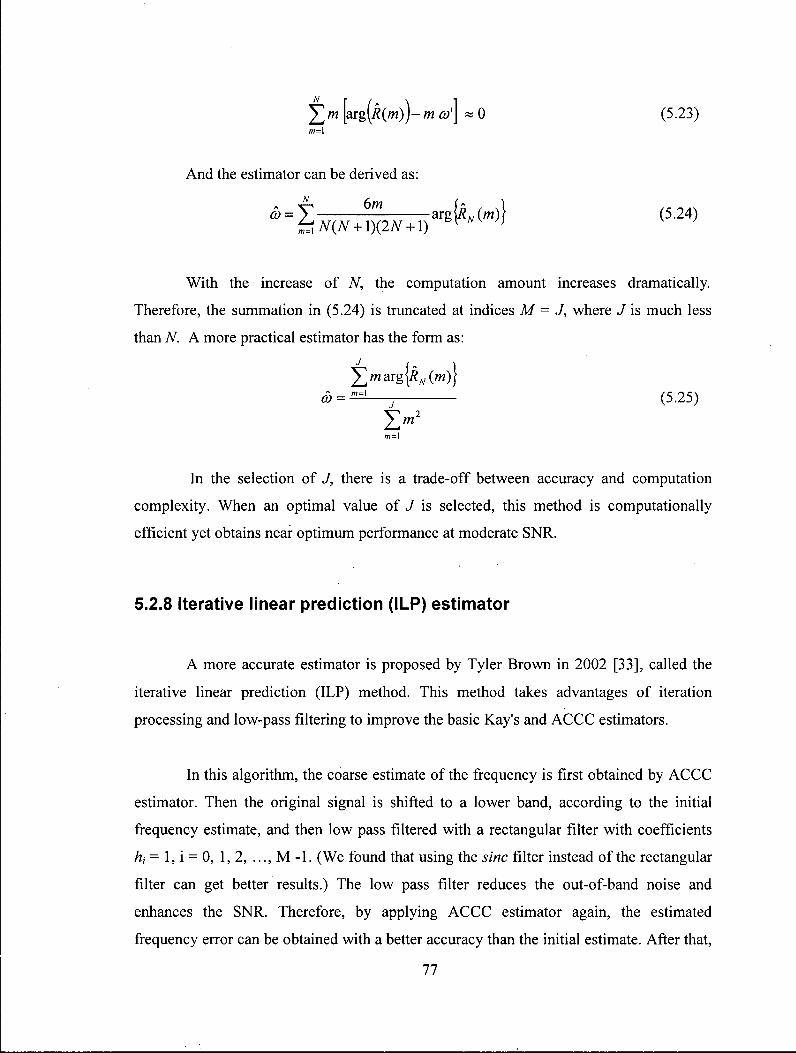
-mco'\ «0 (5.23) m=l

And the estimator can be derived as: N 6m

4 - Z N(N + \)(2N + l) arg (5.24)

With the increase of N, the computation amount increases dramatically.

Therefore, the summation in (5.24) is truncated at indices M = J, where J is much less

than N. A more practical estimator has the form as:

In the selection of J, there is a trade-off between accuracy and computation

complexity. When an optimal value of J is selected, this method is computationally

efficient yet obtains near optimum performance at moderate SNR.

5.2.8 Iterative linear prediction (ILP) estimator

A more accurate estimator is proposed by Tyler Brown in 2002 [33], called the

iterative linear prediction (ILP) method. This method takes advantages of iteration

processing and low-pass filtering to improve the basic Kay's and ACCC estimators.

In this algorithm, the coarse estimate of the frequency is first obtained by ACCC

estimator. Then the original signal is shifted to a lower band, according to the initial

frequency estimate, and then low pass filtered with a rectangular filter with coefficients

hi••= 1 , i = 0, 1 , 2, M - 1 . (We found that using the sine filter instead of the rectangular

filter can get better results.) The low pass filter reduces the out-of-band noise and

enhances the SNR. Therefore, by applying ACCC estimator again, the estimated

frequency error can be obtained with a better accuracy than the initial estimate. After that,

co = m=l (5.25)

I>2

77

the coarse frequency estimate is corrected by the estimated frequency error and the next

iteration starts by shifting the original signal with the corrected frequency estimate. After

each iteration, the bandwidth of the low-pass filter is reduced by two. In this way, the

SNR is enhanced by a narrower filter bandwidth, which improves the estimation

accuracy. Therefore, by iteratively applying the ACCC estimator, the procedure can

reduce the error of the estimated frequency at each iteration. The iterative procedure can

be ended when there is no significant improvements detected or the bandwidth of the low

pass filter is smaller than the bandwidth of the beat signal.

The iterative calculation and frequency estimate at iteration k are given by:

xk (n) = exp(-7© t_,«) x(n)

Mk-\

v*00= Z X k ( M k n + ™)> « = 0 , 1 , ... , N

m=0 Mk-\

Am, = 1

-arg NIMk-\

v\(n-\)vk(n)

(5.26)

(5.27)

(5.28)

d>k=(Mk+a>k_x)'_ (5.29)

where cbQ is the initial estimate of the basic Kay's estimator, vk (n) is the signal after low-

pass filtering, Ad>k is the estimated frequency error in the current iteration, and cbk is the

corrected frequency estimate in the current iteration.

As the analysis above, the ILP estimator improve the performance of the basic

estimators by iteratively applying low-pass filters. As the bandwidth of the low-pass

filter is reduced at each iteration, the frequency estimate is getting more and more

accurate. Consequently, the ILP estimator has the best performance among the survey

results of frequency estimators.

78

5.2.9 Simulations of single frequency estimators

To test and compare the performance of the discussed frequency estimators, we

simulate a single frequency signal with white noise and use these estimators to measure

the frequency separately. In this experiment, we use Mean Square Error (MSE) as the

accuracy measurement. The MSE is defined as the average of the square of the difference

between the estimated frequency and the actual frequency, which can be calculated as:

which is defined as

where E[ ] is the calculation of expectation, 6> is the estimated frequency, and cotrue is the

true frequency.

( 5 . 3 0 )

70

HLC Estimator

|> ILP Estimator -10

-15 -10 -5 0 5 SNR (dB)

10 15 20 25

Figure 5-6 Comparison of single frequency estimators

79

Figure 5-6 shows the estimation results of all the frequency estimators for

comparison. In Figure 5-6, it can be seen that all the estimators suffer from the SNR

threshold. As we discussed before, the SNR threshold is defined as the SNR value, below

which the estimate accuracy decreases dramatically. As illustrated in the figure, the SNR

threshold of the ILP estimator is about -4 dB; the SNR thresholds of the FFTs estimators

(including the estimator using Center of Gravity) are about -7 dB despite of the FFTs

length; the SNR threshold of the FCFB estimator is about 6 dB; and the SNR threshold of

the High Lag Correlation estimator is about 0 dB. In addition, the ACCC estimator does

not appear to exhibit a sharp SNR threshold but gradually deteriorates in performance

with decreasing SNR. The results show that the estimation algorithms based on

periodogram have a relatively lower SNR threshold. Moreover, the estimation error of the

estimator using the maximum FFT coefficient keeps constant beyond the SNR threshold

due to the quantization errors. Even using the Center of Gravity, the estimate results of

the FFT methods still cannot get an approach to the Cramer-Rao Bound as close as the

algorithms based on phase increments. Considering the closeness to the Cramer-Rao

Bound as well as the SNR threshold, we can come to the conclusion that the ILP

estimator is the best algorithm for the single frequency estimation problem among all the

estimators in this study.

5.3 The Beat Frequency Estimation

As discussed in Section 5.1, the beat signal can be approximated by a single-

frequency narrow-band signal. Therefore, the frequency estimators discussed in Section

5.1 can be applied to the beat frequency estimation. However, as the existence of noise,

the bandwidth, and the cross beating, the accuracy of the beat frequency estimation is not

as good as in the ideal condition.

80

5.3.1 The application of the frequency estimators

If we use the beat frequency,/^ in (5.2), to substitute the linear term in (5.1), and

ignore the quadratic term, the beat signal with additive noise can be expressed in discrete

time as:

Shea, O ) ~ ^(")eXp f f

j2n J^L^n \ + z(n) V PRF j

H = 0,1,2, ...,N-\

(5.31)

where n is the azimuth time index, A(n) is the azimuth envelope, and z(n) is the complex

noise with variance a 2 .

So, comparing the beat signal in discrete time (5.31) to the single frequency signal

model (5.6), the frequency estimators can be applied directly to the beat signal. Using the

basic Kay's estimator, the estimated beat frequency has the similar form as in (5.16) ,

which is given by:

PRF ^ fbeat = X, ^ A "g^ t e * (")} ( 5 J 2 )

2n „ = 0

where w(ri) is the same weighting function as in (5.17).

Similarly, other phase-based frequency estimators can be applied to the beat

frequency estimation. In those estimators, the ILP estimator is expected to have the best

performance. The estimated beat frequency using the ILP estimator can be obtained by

the following calculation:

f lk)=Af {k) + f (* _ , ) (5 331 J beat ^Jbeal ^ J beat W ' J : , i

where) fbeJ° is the initial estimate of the basic Kay's estimator, A f b e a , ( k ) is the

estimated frequency error in the current iteration, and fbeJk) is the frequency estimate in

the current iteration after correction.

81

With the estimate of the beat frequency, the absolute Doppler centroid frequency

and the Doppler ambiguity can be obtained using the same procedure as in the existing

MLBF algorithm, described in Chapter 3.

5.3.2 Quality criteria

In order to avoid corruption by bad estimates from the areas with very weak

backscatter or low contrast, quality criteria can be used to detect and remove bad

estimates from the final absolute Doppler estimate, when the "spatial diversity" approach

[19] is used. In addition to the data quality criteria of SNR and contrast used in [19], two

other estimator quality criteria that are specific to the operation of the beat frequency

estimators were examined:

Peak to Mean Ratio (PMR)

In the frequency estimators based on FFTs, the periodogram can be checked for

quality. A good periodogram with a sharp and clear peak would give a good frequency

estimate. Therefore, by checking the shape of the periodogram, we can obtain the

measurement of how good the frequency estimate could be. A quality criterion "Peak to

Mean Ratio (PMR)" is introduced for this purpose. As shown in Figure 5-7, the Peak to

Mean Ratio is defined as the ratio between the global peak and the mean value of the non-

peak area in the periodogram. The peak area is the area within the 10 dB bandwidth

downward from the peak of the main lobe, and the non-peak area is the remaining area

other than the peak area. This ratio is usually expressed in dB units, and is given by:

PMR = 20 log f P e a k

g l o b a l

KMeannon_peak ;

(5.34)

82

Magnitude

Global Peak

Mean of non-Peak area

Azimuth frequency

Figure 5-7 Measurement of PMR

Phase Coherence

In the estimators based on phase increments, the more consistent the phase

increments are, the better estimates can be obtained. Hence, in this case the phase

coherence is found to be the most appropriate quality measurement [34]. The phase

coherence measures the consistency of the phase increments of the beat signal. It is

defined as the ratio between the absolute value of the summation and the summation of

the absolute value of the vectors that contains the phase increments, and can be expressed

as:

\N-2

£ s\eal (n)sbeal 0 + 1)

Ph coher -N-2 (5.35)

where sbea*(ri) sbeal (n +1) is the correlation of the beat signal, whose phase is the phase

increments of the beat signal.

83

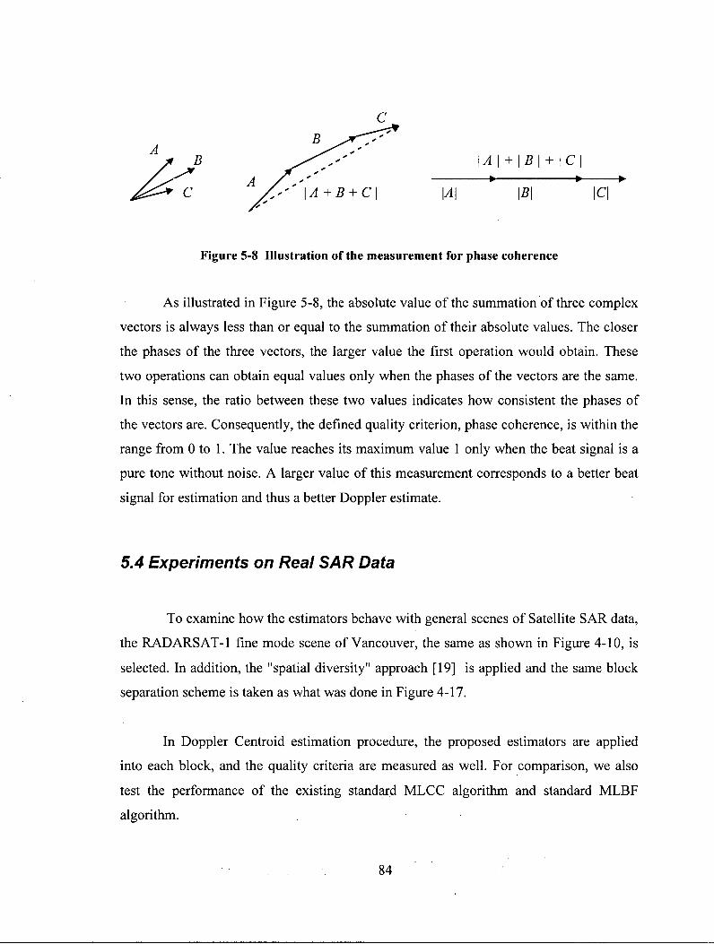
Figure 5-8 Illustration of the measurement for phase coherence

As illustrated in Figure 5-8, the absolute value of the summation of three complex

vectors is always less than or equal to the summation of their absolute values. The closer

the phases of the three vectors, the larger value the first operation would obtain. These

two operations can obtain equal values only when the phases of the vectors are the same.

In this sense, the ratio between these two values indicates how consistent the phases of

the vectors are. Consequently, the defined quality criterion, phase coherence, is within the

range from 0 to 1. The value reaches its maximum value 1 only when the beat signal is a

pure tone without noise. A larger value of this measurement corresponds to a better beat

signal for estimation and thus a better Doppler estimate.

5.4 Experiments on Real SAR Data

To examine how the estimators behave with general scenes of Satellite SAR data,

the RADARSAT-1 fine mode scene of Vancouver, the same as shown in Figure 4-10, is

selected. In addition, the "spatial diversity" approach [19] is applied and the same block

separation scheme is taken as what was done in Figure 4-17.

In Doppler Centroid estimation procedure, the proposed estimators are applied

into each block, and the quality criteria are measured as well. For comparison, we also

test the performance of the existing standard MLCC algorithm and standard MLBF

algorithm.

84

5.1.1 Examining the quality criteria

In this experiment, SNR, PMR of the periodogram and the phase coherence are

measured as the quality criteria of the estimators to remove the possible bad estimates.

For the Vancouver scene, the true Doppler ambiguity number is -6. So the good quality

criteria should keep the blocks with correct Doppler ambiguity estimates and remove the

blocks with incorrect Doppler ambiguity estimates as many as possible.

Table 5-1 Examining quality criteria with M L B F using I L P estimator

Quality Criteria Number of blocks with

Good estimate

Number of blocks with

Bad estimate

SNR>-2.8dB 172 30

SNR < -2.8 dB 7 19

PMR> 1.5 dB 170 30

PMR < 1.5 dB 9 19

Phase Coherence > 0.17 175 30

Phase Coherence < 0.17 4 19

Table 5-1 shows how the quality criteria behave in recognizing the blocks with

good estimates from those with the bad estimates. It can be seen that a threshold can be

chosen that does a reasonable job of separating those blocks that yield good estimates

from those blocks that give bad estimates. In this experiment, we adjust the thresholds so

the number of blocks excluded is the same for each criterion. From the result, it can be

seen that the quality criterion of the phase coherence with a threshold at 0.17 shows the

best performance in rejecting the possible bad estimates while keeping the good

estimates. In this case, 21 blocks out of total 228 blocks (about 10%) are rejected.

85

5.4.1 Results of Doppler ambiguity estimates

After removing the possible bad estimates, the final Doppler ambiguity estimate

can be obtained by an average or "majority vote" operation. The estimate results of all the

estimators within the remaining 207 blocks are listed in Table 5-2. In this table, the

ambiguity error before rounding, the standard deviation, and the success rate of the

correct estimates are considered as the measurements of the estimator's performance. We

consider the standard deviation as the best parameter to evaluate the estimator because it

shows how the estimate results disperse around the true value and it's the most direct

measurement of the randomness of the estimator. In addition, it is worth noting that since

there are many bright isolated targets in the Vancouver scene, the estimate results of

MLBF algorithm are much better than those of MLCC algorithm.

Table 5-2 Comparison of Doppler ambiguity resolvers for the Vancouver data

Doppler Ambiguity Resolvers Mean (PRFs)

St. Dev. (PRFs)

Success rate (%)

Standard MLCC -5.99 1.36 41

Standard MLBF -5.72 1.09 62

MLBF using Center of Gravity -5.75 0.92 69

MLBF using Kay's -5.95 0.92 55

MLBF using ACCC -6.02 0.90 57

MLBF using HLC -5.94 0.75 63

MLBF using FCFB -5.88 0.83 56

MLBF using ILP -5.89 0.43 85

Figure 5-9 shows the histogram of the Doppler ambiguity estimates by using

different Doppler ambiguity resolvers. It illustrates the same results as shown in Table 5-2

86

in a more visible way. The height of the peak at the correct ambiguity number corresponds to the success rate, and the spread of the "bars" is related to the standard deviation of the estimates. The symmetry of the bar chart is very important to get the correct average (mean).

Standard MLCC Standard MLBF

-10 -5 0

MLBF using Cen-of-Grav

MLBF Using Kay's

i . -15 -10 -5

MLBF Using High Lag Corr

MLBF Using ACCC

MLBF Using FCFB

150

100

50

-15 -10

MLBF Using ILP

-10 Ambiguity Number Ambiguity Number

Figure 5-9 Histogram of the Doppler ambiguity estimates by DARs

of the 207 selected blocks

87

It can be seen in Table 5-2 as well as in Figure 5-9 that the frequency estimators

using the phase increments have lower standard deviation than the estimators using FFTs.

It means that the frequency estimators show better performances than the existing

frequency estimators in the MLBF algorithm. Especially, the ILP estimator has the best

performance among all the estimators. It has the lowest standard deviation (less than half

of the existing estimator) as well as the highest success rate (23% higher than the existing

estimator). So, in implementation, we recommend to apply the ILP estimator in the beat

frequency estimation in the MLBF algorithm.

5.5 Summary

In this chapter, we applied improved beat frequency estimation methods to the

MLBF algorithm for the Doppler ambiguity resolution. As the existing MLBF algorithm

uses the maximum FFT coefficient to measure the beat frequency, the estimate accuracy

is limited by the quantization errors and RCM segmentation. As a survey result, several

frequency estimators are introduced to avoid such quantization errors. We first analyzed

and examined the estimator based on the center of gravity in the periodogram. Then, we

introduced and compared five frequency estimators that are based on phase increments.

To improve the beat frequency estimation, we applied the frequency estimators discussed

with better accuracy in the MLBF algorithm. The experimental results on RADARSAT-1

real data show that the proposed method gives more consistent estimates than the existing

MLBF algorithm. It can achieve correct Doppler ambiguity estimates in a higher

percentage of the blocks and its estimation error is less than half that of the existing

algorithm.

88

Chapter 6 Improved Slope Estimation for Doppler Ambiguity Resolution

The Look Misregistration algorithm proposed in 1986 [10] uses the fact that the

average slope of the target trajectory before range cell migration correction (RCMC) is

proportional to the beam squint angle and the Doppler centroid. Consequently, the

Doppler centroid frequency can be estimated by measuring the slope of the target

trajectory in range compressed image. Kong et al. have proposed to apply the Radon

Transform in the slope estimation to estimate the Doppler centroid frequency of airborne

SAR data in 2005 [35]. In this chapter, Kong's method is well explained and adapted for

Doppler ambiguity resolution for satellite SAR data. In addition, a simpler method of

combining RCMC and integration in slope estimation is presented. Through the

experiments on real data, both the Radon method and the new method prove to have good

performances in estimating the Doppler ambiguity number for satellite SAR data, not

only in scenes with bright isolated targets, but also in the areas with low to medium

contrast.

6.1 Geometry of a SAR Target Trajectory

As discussed in Chapter 2, the Doppler centroid can be derived from the

geometry model of the SAR system; with an accurate knowledge of the system

parameters such as the satellite attitude (see Appendix 12A of [15]). The geometry model

of the SAR system is shown in Figure 6-1, where Vr the effective. SAR is forward

velocity, and 6rc is the beam squint angle measured in the slant range plane. If we know

the parameter values, the total Doppler centroid fnc can be expressed as:

89

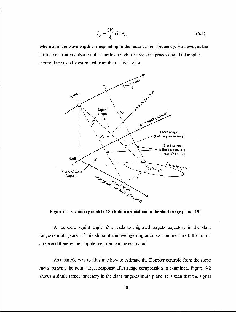
f7c 2V

r (6.1)

where Xc is the wavelength corresponding to the radar carrier frequency. However, as the

attitude measurements are not accurate enough for precision processing, the Doppler

centroid are usually estimated from the received data.

Figure 6-1 Geometry model of SAR data acquisition in the slant range plane [15]

A non-zero squint angle, dr<c, leads to migrated targets trajectory in the slant

range/azimuth plane. If this slope of the average migration can be measured, the squint

angle and thereby the Doppler centroid can be estimated.

As a simple way to illustrate how to estimate the Doppler centroid from the slope

measurement, the point target response after range compression is examined. Figure 6-2

shows a single target trajectory in the slant range/azimuth plane. It is seen that the signal

90

energy can be spread over several range cells during the exposure time. The variation of

range with time is called Range Cell Migration (RCM). As the direction of the beam

center line is perpendicular to the target trajectory at the middle of the target exposure, the

squint angle, dr,c, is equal to the angle of the linear component of RCM.

Azimuth

Satellite antenna

Target trajectory

Beam center line

Slant range (satellite to target)

Figure 6-2 Range migration of a point target in range compressed domain

To illustrate variation of the slant range with time, the slant range equation is

examined. We expand the equation of the slant range about the beam center crossing time

Y]c and ignore the higher order components. Then the range from the satellite to the target

at certain azimuth time, R(r\), can be approximated by the parabola:

lK r

2 cos 2 0 r c

R(r?) = R(rjc)-Vr sin6rfi (rj - 7c) + - r>c (rj-rjj2 (6.2)

From (6.2), we see that the average RCM slope can be expressed as - Vr sin 8rc,

in units of m/s. If the slope is positive, that is, the range increases with azimuth time, the

antenna has a "backward" or negative squint angle - the Doppler frequency is negative, as

is typical of ascending orbits without yaw steering. On the other hand, a negative slope

corresponds to a forward squint angle of the antenna.

91

Therefore, if the RCM slope is measured correctly, the absolute Doppler centroid

can be derived directly from (6.1), with the knowledge of the radar wavelength, X and

satellite effective velocity, Vr. While there are more accurate ways of estimating the

baseband Doppler centroid, the methods of measuring the RCM slope can provide a

reliable estimate of the Doppler ambiguity number.

In this chapter, we introduce two Doppler ambiguity resolvers based on the RCM

slope estimation. One is using the Radon Transform, and the other is using RCMC and

azimuth integration.

6.2 Using the Radon Transform

The Radon Transform is a well-known method of detecting linear features in an

image, such as the slope of lines [36] [37]. Kong et al. have applied the Radon Transform

to estimate the Doppler centroid frequency of airborne SAR data in 2005 [35]. In this

section, we explain Kong's method in more detail and apply it to the Doppler ambiguity

estimation for satellite SAR data. In addition, a few improvements are proposed.

6.2.1 The Radon transform for linear feature detection

In order to extract the information of RCM slope from the range compressed

image, certain image processing techniques can be applied. The Radon transform is an

effective technique in extracting the parameters of linear features, such as their slope,

even in the presence of noise [36] [37]. Because of its advantageous property in detecting

lines with arbitrary orientation, the Radon transform has been successfully used in the

SAR imagery processing, such as ship wake detection [38]. This transform integrates

intensity along every possible direction in the image and maps this information into a

feature space parameterized by the angle with respect to the positive y-axis, 0, and its

distance from the origin, p.

92

The angle, 6, and the distance, p, form the coordinates in the transformed

representation of a line. The concept is that a concentrated point in the transform space

represents a linear feature in the image. This approach is particularly suited for noisy

images, since the integration process tends to average out intensity fluctuations due to

noise. The Radon transform equation for the image, g(x, y), is defined as [36]:

g(p,0) = f f g(x,y)8(p-xcosd - ysm6)dxdy (6.3)

where 8 is the Dirac delta function and d( p - x cosd - y sinO) directs the integration

along the angle, 6. The range of 6 is limited to 0 < 6 < n.

To illustrate the relationship between the image coordinates, (x, y), and the

transform parameters, (6, p), a range compressed SAR magnitude image with three point

targets is simulated in Figure 6-3 Panel (a). A significant linear RCM is assumed, and the

quadratic RCM is negligible. The skew angle of the target trajectories is 30 degree, and

the Radon transform is taken over angles from 28 to 32 degrees, in steps of 0.2 degrees.

The transform result is shown in Panel (b), where only the central part of the p axis is

displayed. When the integration in (6.3) is taken along the true direction of the lines, the

energy is most concentrated along the p axis. It can be seen that there are three

concentrated areas of energy in the vicinity of 6 = 30°, which indicates the angle of the

skewed lines in the image.

93

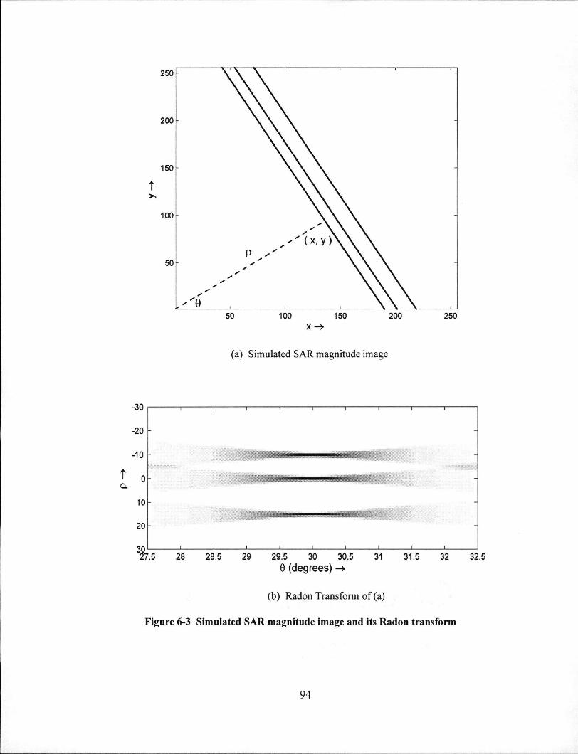
50 100 150 200 250

X - >

(a) Simulated SAR magnitude image

(b) Radon Transform of (a)

Figure 6-3 Simulated SAR magnitude image and its Radon transform

9 4

In order to investigate the results in more detail, we take vetical slices along the p

axis of Figure 6-3 Panel (b) at several angles. Figure 6-4 shows those five slices from 26

degree to 32 degree. It can be seen that the Radon Tranform result is highly concentrated

at the actual skew angleof the target trajectories and increasingly dispersed at other

angles. In this way, the RCM slope in the range-compressed SAR image can be estimated

by finding the skew angle, 6, that gives the maximum concentration of the Radon

Transform energy along the p axis. A detection method of the Feature Space Line

Detector (FSLD) was proposed in [37], which it was shown that the calculation of the

variance of the slices along the p axis is a good measurement of the concentration.

Figure 6-4 Vertical slices through Radon transform of Figure 6-3 Panel (b)

6.2.2 Applying the Radon transform to Doppler estimation

Due to its ability of detecting the linear features in an image, Kong et al. applied

the Radon transform into Doppler centroid estimation of airborne SAR data in their

geometry Doppler estimator (GDE) [35]. However, due to the lack of bright isolated

targets in most real SAR data, the measurements are usually not precise enough for the

estimation of the baseband part of the Doppler centroid. Since there are several

95

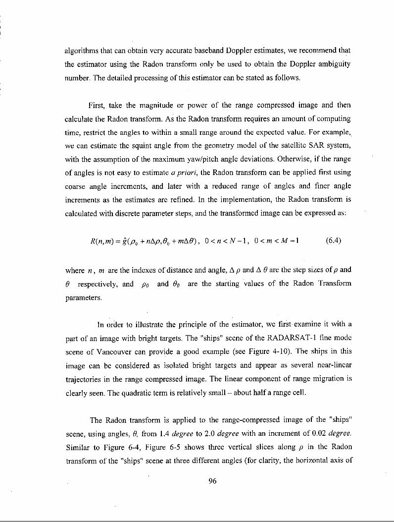
algorithms that can obtain very accurate baseband Doppler estimates, we recommend that

the estimator using the Radon transform only be used to obtain the Doppler ambiguity

number. The detailed processing of this estimator can be stated as follows.

First, take the magnitude or power of the range compressed image and then

calculate the Radon transform. As the Radon transform requires an amount of computing

time, restrict the angles to within a small range around the expected value. For example,

we can estimate the squint angle from the geometry model of the satellite SAR system,

with the assumption of the maximum yaw/pitch angle deviations. Otherwise, if the range

of angles is not easy to estimate a priori, the Radon transform can be applied first using

coarse angle increments, and later with a reduced range of angles and finer angle

increments as the estimates are refined. In the implementation, the Radon transform is

calculated with discrete parameter steps, and the transformed image can be expressed as:

R(n,m) = g(p0 + nt\p,0o + mA0), 0<n<N -1 , 0 <m < M -1 (6.4)

where n, m are the indexes of distance and angle, A p and A 6 are the step sizes of p and

0 respectively, and po and do are the starting values of the Radon Transform

parameters.

In order to illustrate the principle of the estimator, we first examine it with a

part of an image with bright targets. The "ships" scene of the RADARSAT-1 fine mode

scene of Vancouver can provide a good example (see Figure 4-10). The ships in this

image can be considered as isolated bright targets and appear as several near-linear

trajectories in the range compressed image. The linear component of range migration is

clearly seen. The quadratic term is relatively small - about half a range cell.

The Radon transform is applied to the range-compressed image of the "ships"

scene, using angles, 6, from 1.4 degree to 2.0 degree with an increment of 0.02 degree.

Similar to Figure 6-4, Figure 6-5 shows three vertical slices along p in the Radon

transform of the "ships" scene at three different angles (for clarity, the horizontal axis of

96

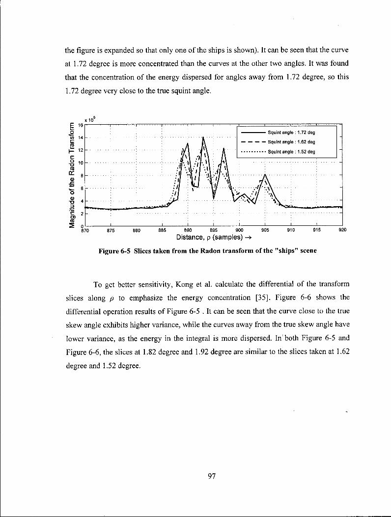
the figure is expanded so that only one of the ships is shown). It can be seen that the curve

at 1.72 degree is more concentrated than the curves at the other two angles. It was found

that the concentration of the energy dispersed for angles away from 1.72 degree, so this

1.72 degree very close to the true squint angle.

870 875 880 885 890 895 900 905 910 915 920

Distance, p (samples) ->

Figure 6-5 Slices taken from the Radon transform of the "ships" scene

To get better sensitivity, Kong et al. calculate the differential of the transform

slices along p to emphasize the energy concentration [35]. Figure 6-6 shows the

differential operation results of Figure 6-5 . It can be seen that the curve close to the true

skew angle exhibits higher variance, while the curves away from the true skew angle have

lower variance, as the energy in the integral is more dispersed. In both Figure 6-5 and

Figure 6-6, the slices at 1.82 degree and 1.92 degree are similar to the slices taken at 1.62

degree and 1.52 degree.

97

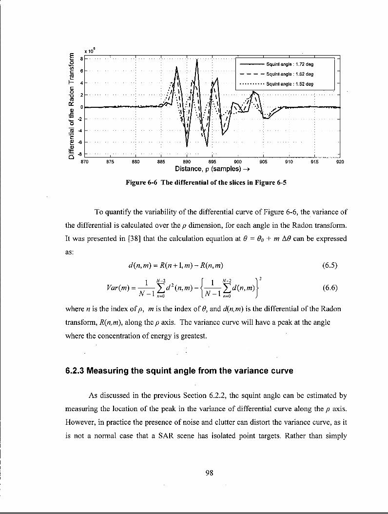
870 875 880 885 890 895 900 905 910 915 920

Distance, p (samples) H>

Figure 6-6 The differential of the slices in Figure 6-5

To quantify the variability of the differential curve of Figure 6-6, the variance of

the differential is calculated over the p dimension, for each angle in the Radon transform.

It was presented in [38] that the calculation equation at 9 = Oo + m AO can be expressed

as:

d(n,m) = R(n + \,m)-R(n,m) (6.5)

Var ( H I ) = -J— X d2 (/i, m) -1-*- £ d(n, m)\ (6.6)

where n is the index of p, m is the index of 6, and d(n,m) is the differential of the Radon

transform, R(n,m), along the p axis. The variance curve will have a peak at the angle

where the concentration of energy is greatest.

6.2.3 Measuring the squint angle from the variance curve

As discussed in the previous Section 6.2.2, the squint angle can be estimated by

measuring the location of the peak in the variance of differential curve along the p axis.

However, in practice the presence of noise and clutter can distort the variance curve, as it

is not a normal case that a SAR scene has isolated point targets. Rather than simply

98

finding the peak of the variance curve, a curve fitting approach can find the central angle

more accurately.

Kong et al. have recommended using a Gaussian function with four unknown

parameters to fit the variance curve and measure the peak location from the fitting

parameters. The Gaussian function is defined as:

G(x) = A exp f ( * - / Q 2 > >

2a2 + C (6.7)

where x is the independent angle variable, and the four unknown parameters are: the

amplitude, A, the mean or peak location parameter p., the standard deviation, a, and the

additive constant (pedestal), C.

In the definition, a certain Gaussian function can be fully expressed by the four

parameters: A, /u, a, and C. After finding a set of parameters that can form a Gaussian

function with a closest shape to the actual curve, the peak location of the curve can be

measured from the mean value \x. Figure 6-7 shows the curve fit procedure.

Variance

Angle 0

Figure 6-7 Fitting a Gaussian function to the variance curve

99

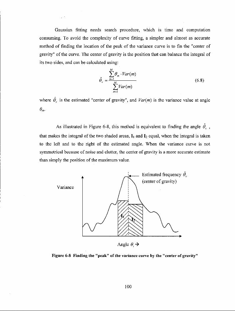
Gaussian fitting needs search procedure, which is time and computation

consuming. To avoid the complexity of curve fitting, a simpler and almost as accurate

method of finding the location of the peak of the variance curve is to fin the "center of

gravity" of the curve. The center of gravity is the position that can balance the integral of

its two sides, and can be calculated using:

YO.-Varim) I (6-8)

^Far (m) m=l

where 6C is the estimated "center of gravity", and Var(m) is the variance value at angle

0m-

A s illustrated in Figure 6-8, this method is equivalent to finding the angle Gc ,

that makes the integral of the two shaded areas, I i and I2 equal, when the integral is taken

to the left and to the right of the estimated angle. When the variance curve is not

symmetrical because of noise and clutter, the center of gravity is a more accurate estimate

than simply the position of the maximum value.

100

To test the performances of the two measurements, we implement them with the

"ships" scene. In the implementation, we use MATLAB's fminsearch routine to find

the four unknown parameters for the Gaussian fit. This routine uses the Nelder-Mead

parameter search procedure [39]. Figure 6 -9 shows the measurement results of the

Gaussian fit and center of gravity for the "ships" scene. Because the variance curve is

quite symmetrical and the noise level is low in this high contrast case, the Gaussian fit

curve is very close to the actual variance curve. The closeness of the fit curve shows that

the Gaussian function is an appropriate fitting function for this SAR data. It is also shown

in the figure that using Gaussian fit the measured squint angle is 1.726 degree, and using

the center of gravity the measured squint angle is 1.731 degree. Both of the measurements

are very close to the true squint angle of 1.720 degree. While the Gaussian fitting method

obtains the best estimate in this case, the error of the center of gravity method is fairly

small, well within the ambiguity error limit (the ambiguity error limit represents the range

of angles that do not lead to a Doppler ambiguity error). In summary, the Gaussian fitting

method can give the best squint angle measurement. The center of gravity method can be

viewed as a simpler but still adequate way.

1.4 1.5 1.6 1.7 1.8 1.9

Squint Angle (degrees) -»

Figure 6-9 Estimating the squint angle from the variance curve ("ships" scene)

101

6.2.4 Resolving the Doppler ambiguity

However, the estimated squint angle is in the unit of range samples per azimuth

sample and needs to be changed into unit of meters per second. So, the estimated angle is

multiplied by c /(2Fr) to change range samples into meters and by the PRF to change

azimuth samples into seconds. After the adjustments, the result is measured in the same

unit of the squint angle of the radar beam and the Doppler centroid can be calculated

directly from (6.1).

As in other Doppler ambiguity resolvers, the baseband Doppler Centroid should

be measured first using "spectral fit" or ACCC algorithm [15]. Then, the baseband

Doppler centroid is subtracted from the estimated absolute Doppler frequency and the

result is divided by the PRF. After this, the ambiguity estimate is obtained by a rounding

operation. This reduces the ambiguity estimate to the more reliable estimate of an integer.

The calculating procedure can be expressed as [15]:

Mamb = round] r f _ f <\ J rjc J rjc

PRF

(6.9)

where fvc is the absolute Doppler frequency estimate from the Radon method, fnc' is the

accurate baseband Doppler centroid estimate, and Mamt is the estimated ambiguity

number.

6.2.5 Discussion

In this subsection, two SAR signal processing procedure are discussed that would

provide some improvements to the Radon estimation method.

Removing Quadratic RCM

As shown in (2.6) of Chapter 2, the RCM is not a purely linear function and the

quadratic components of RCM cannot be ignored in some SAR system. If the quadratic

RCM is significant, the estimated slope will vary along the target trajectory and the peak

102

of the variance curve will be further dispersed, reducing the sensitivity of the estimator.

Therefore, in order to adjust the RCM to a straight line, it is recommended to remove the

quadratic part from the full RCM before applying the Radon Transform.

The quadratic RCM in meters in azimuth time domain can be expressed as:

V2cos20rc , V2

A ^ ( 7 ) = ' :-c(rj-rjc)2 « - _ ^ ( 7 - 7 c ) 2 (6.10)

where the approximation is used when the squint angle, 6rx, is small enough and cos2 6r,c

can be approximated by 1. The variable rjc is the beam center crossing time and R{rjc) is

the slant range at the time when the target is illuminated by the beam center.

Fortunately, for most C-Band satellite SAR systems, such as RADARSAT-1 and

ENVISAT, the quadratic part of RCM is relatively small. For example, in the "ships"

scene that is acquired by the F2 beam of RADARSAT-1, the maximum quadratic RCM is

about one half a range cell. Hence, removing the quadratic RCM would not lead to a

significant improvement in this case. But for L-band satellites data, the quadratic part of

RCM could be as large as several cells, and removing this part will improve the estimator

considerably. It is also worth noting that the quadratic component of RCM can only be

efficiently removed in the azimuth frequency domain and that the Radon method can be

adapted to operate in this domain.

Secondary Range Compression

Depending upon the radar system parameters and the squint angle, secondary

range compression (SRC) may have to be applied to sharpen the focus in the range

Doppler domain. As discussed in Chapter 6 of [15], without SRC the range-compressed

image can be defocused in the azimuth frequency domain, even though it is well focused

in the azimuth time domain. On the other hand, if SRC is applied with the range

compression filter, the image is well focused in the azimuth frequency domain, but

possibly defocused in the azimuth time domain.

103

Therefore, if we apply the Radon Transform into RCM slope detection in the

azimuth time domain (as we do in the examples in this Chapter), SRC should be

implemented after the estimator. Otherwise, if RCM slope is detected in the azimuth

frequency domain, SRC should be implemented before the estimator.

6.2.6 Quality Criteria

In order to avoid the corruption of the bad estimates from the areas with very

weak backscatter or low contrast, quality criteria are used to detect and remove bad

estimates from the final estimate, when the "spatial diversity" approach [19] is applied. In

addition to the common quality criteria of SNR and contrast used in [15], four other

estimator quality criteria that are specific to the estimator using the Radon Transform are

examined as following:

Gaussian fit flag

This flag is to indicate whether the Gaussian fit method can achieve a expected

fitting curve. If the search for the four Gaussian fit parameters does not converge, the fit

procedure fails and the MATLAB 1 fminsearch' routine will come out with an error

flag (flag = 0). In addition, if the fit parameters are beyond a reasonable range, we also

declare that the fit procedure fails and set the flag to zero. On the other hand, if the fit is

deemed successful, the flag is set to one and the next three criteria are examined.

Fit distortion (Fit std)

The Fit distortion is defined as the normalized standard deviation of the difference

between the measured variance curve and the fitting Gaussian function. This quality

parameter is used to measure how close the shape of the variance curve to the Gaussian

function. If the fit distortion has a fairly small value, it means that the variance curve is

well-shaped and most possibly can provide a good estimate. On the contrary, if the fit

distortion has a relatively large value, it means that the variance curve is distorted

considerably and may provide a bad estimate.

104

Peak to Pedestal Ratio (PPR)

In addition, the shape of the fitted Gaussian function can be used to measure how

good the estimate is. The Peak to Pedestal Ratio is obtained from the Gaussian fitting

parameters by PPR = (A+Q I C. This quality parameter is used to measure the relative

height of the peak. The bigger the ratio, the more outstanding the peak, and consequently

the better the estimate.

Width of Gaussian fit

The parameter of standard deviation, er, of the Gaussian function gives the width

of the Gaussian fit. It is used to measure the sharpness of the variance curve. As we

assume that sharper variance curves indicate better the estimates, it is preferred that the

width of Gaussian fit has a smaller value.

6.3 Using the RCMC and Integration

The Doppler ambiguity resolver using the Radon Transform is a reliable method

to obtain Doppler ambiguity estimates. However, the Radon Transform requires large and

complex computations. In this section, we propose a new Doppler ambiguity resolver

using RCMC and integration, which is based on the similar principle as the algorithm

using the Radon transform but only requires simple calculations. Similar to the algorithm

using the Radon Transform, this estimator cannot provide accurate baseband Doppler

centroid frequency, but has good performance in Doppler Ambiguity estimation.

6.3.1 RCMC and azimuth integration

As discussed in the Section 6.2.2, the slope of the target trajectories with residual

Range Cell Migration (RCM) is proportional to the Doppler centroid. In the proposed

algorithm, RCMC is used to change the slope of the targets trajectories, and the azimuth

integration is used to measure straightness of the trajectories along azimuth.

105

The absolute Doppler centroid frequency consists of baseband Doppler centroid

part and Doppler Ambiguity part, which can be expressed by:

where f„c is the baseband Doppler centroid frequency, Mamb is the ambiguity number.

In this algorithm, in order to resolve the correct Doppler ambiguity number,

correct baseband Doppler centroid estimates, fnc', are required. The coarse baseband

Doppler estimates can be obtained by baseband Doppler estimators, such as "spectral fit"

and ACCC algorithms. Then, the baseband Doppler is found as a function of range over

the whole scene and unwrapped over the PRF jumps. In addition, the possible range of

the Doppler ambiguity number is estimated from the geometry model, with the

assumption of the maximum satellite attitude variation. As a result, a set of candidate

absolute Doppler centroid frequencies is obtained from (6.11) according to the Doppler

ambiguity range.

After that, full RCMC (e.g., both the linear and quadratic parts) is applied over the

whole range compressed image using the candidate Doppler centroid frequencies. For

processing efficiency, RCMC is usually implemented in range time and azimuth

frequency domain, which is also called the range Doppler domain. In our study, RCMC is

performed by using an interpolator based on the sine function in the range Doppler

domain. The sine kernel is truncated and weighted by Kaiser Window. This equation

represents the target displacement as a function of azimuth frequency fn and the amount of

RCM to correct is given by the second term in (6.10)

where f„c is the absolute Doppler centroid used, X is the signal wavelength, and Vr is the

radar effective velocity.

If RCMC is applied with correct Doppler ambiguity number, the target trajectories

should be sprightly parallel to the azimuth direction and the energy gets most

concentrated in certain range cells. Otherwise, if RCMC is applied with Doppler

fnc=fnc' + MambPRF (6.11)

RCM(fn) = (6.12) %Vr

2

106

ambiguity errors, the target trajectories have residual migration over several range cells,

and the energy is dispersed over those range cells. Therefore, the correct Doppler

ambiguity can be estimated by finding the ambiguity number with which RCMC can fully

remove the RCM and make the target trajectories exactly straight to the range direction.

Applying azimuth integration of the data magnitude or power is found to be an

effective way to measure the straightness of the target trajectory after RCMC. This

operation is similar to what we do in the Radon Transform when the skew angle is zero. If

the target trajectories are fully straight to the range direction, the energy vs. range is most

concentrated. On the other hand, if the target trajectories have skewed slope along

azimuth, the energy vs. range is dispersed.

To test its performance, the RCMC with azimuth integration method is applied to

the "ships" scene, the same as the one we used in Section 6.2.2. The results of the azimuth

integration using several ambiguity numbers are shown in Figure 6-10. It can be seen that

the result with the most concentrated energy is obtained when the correct ambiguity

number, Mamb = - 6 is used. The results are dispersed, when the ambiguity numbers are

away from the correct number, - 6. The larger the errors, the more dispersed the energy.

107

6.3.2 Finding the Doppler ambiguity

As discussed in Section 6.2.2, the variance is a good parameter to measure the

concentration of the curve. In this estimator, the variance of the integration curve vs. the

Doppler Ambiguity number is calculated. The variance can be obtained by:

Var{m) = —— £ Int2 (n, m) - ——- £ Int(n, m) (6.13)

where m is the index of the Ambiguity number, n is the index of range cell, and Int(n,m)

is the azimuth integration at the specific range cell and ambiguity number.

The correct answer is even more apparent when the differential and variance are

taken over the range variable. These results are plotted in Figure 6-11, which shows that

the RCMC/integration results agree closely with the Radon transform results.

; 5 /

/

\ \

/ \ /

/ /

/ \

\

r

/ /

/

\

\ :

: - - - " ^ —~

J

-8 -6.5 -6 -5.5

Ambiguity number -4.5

Figure 6-11 Variance curve in RCMC/Integration method

6.3.3 Discussion

Essentially, this method replaces the Radon transform with a simple integration of

the image energy over one dimension (azimuth). Only one ambiguity number results in

108

RCMCed data that is aligned accurately in azimuth, and quality checks are an effective

way of checking the accuracy of the alignment.

The baseband centroid estimates must be unwrapped so that a single ambiguity

number applies over the whole scene. The spatial diversity, curve fitting method is the

most reliable way of ensuring accurate estimates that vary smoothly over the scene, and

the unwrapping is correct [19].

The RCMC is best applied in the azimuth frequency domain, as in the range

Doppler algorithm, so that the quadratic RCMC can be performed efficiently. The

subsequent estimation can be done in this domain, which is why SRC should be applied

with the range compression filter (i.e., using Option 3 described in Chapter 6 of [15]).

6.3.4 Quality criteria

As in any ambiguity estimation method, parts of each scene will likely yield bad

estimates. These usually occur in areas of low image SNR and/or low image contrast.

Using the "spatial diversity" approach [19] over small blocks of the scene, quality criteria

can be used to reject the bad blocks and obtain higher confidence in the answer. In

addition to measuring the SNR and contrast of each block, the Peak to Pedestal Ration

(PPR) is a suitable quality parameter.

As described in Section 6.2.4, the quality criteria are measured to remove the bad

estimates. In this algorithm, we examine the quality measurements that are obtained from

the shape of the variance curve. It can be found in the analysis that the sharper the curve

of variance vs. Ambiguity number is, the more isolated targets are contained in the block

and the more accurate estimate would be obtained. Therefore, we use the PMR and

Normalized peak as the quality criteria.

109

Peak to Pedestal Ratio (PPR) Similar to the quality measurement PMR described in Section 5.3.2, this

measurement is used to measure the height of the peak compared to the non-peak values.

The ratio is obtained by dividing the value of the peak point by the mean value of the

other points.

6.4 Experiments on Real Satellite Data

As shown in the simulations and results of "ships" scene, the estimators using the

Radon Transform and the RCMC/integration method have good performances in the area

with isolated bright targets, since the targets have clearly-defined linear features after

range compression. Kong has examined this estimator using the Radon Transform on

three sets of airborne SAR data. In this section, we examine the performances of the

estimators on general scenes of Satellite SAR data with different kinds of terrain. For

comparison with other Doppler Ambiguity solvers, the RADARSAT-1 Vancouver scene

is selected, as shown in Figure 4-10. In this experiment, the "spatial diversity" approach

[19] is applied to obtain a single ambiguity number over the whole scene and the same

block separation scheme is taken as what was done in Figure 4-17.

After range compression, the accurate "spectral fit" baseband Doppler estimator is

applied and the PRF wraparound is removed. The quadratic component of RCM is

removed. Then, the Radon and the RCMC/integration methods are applied to estimate the

Doppler ambiguity. The quality criteria are measured for each block to test their

effectiveness and to remove biased or noisy estimates

6.4.1 Analysis of typical results

Typical results are shown in Figure 6-12. This figure shows the results of the 12

blocks in the first row of the scene. The blocks run in the range direction of the scene, and

are numbered from left to right, starting from the top of the figure. The horizontal axis

refers to the angle used in the Radon transform, but is expressed in units of ambiguity

110

number for compatibility with the RCMC/integration method and for visibility of the

result in ambiguity units. The baseband centroid is removed from the estimate, so the

answer should be an integer. The correct answer is indicated by the vertical solid line and

equals -6, and the vertical dashed lines indicate the ambiguity error limits (exceeding

these limits results in an ambiguity error).

ROW: 1 DopCen Amb Solver based on slope estimation. Aver, area 1024 x 655

-8 -6 - 4 - 8 -6 - 4 - 8 -6 - 4 - 8 -6 Amb = -6 Amb = -6 Amb = -6 Amb = -6 A m b „ = -6 Amb = -6 A m b „ = -6 Amb _ , = -6

-8 -6 - 4 - 8 -6 - 4 - 8 -6 - 4 - 8 -6 -4 Ambiguity number Ambiguity number Ambiguity number Ambiguity number

Figure 6-12 Finding the location of the peak of the variance curve by the Radon transform

(Gaussian fit) method and by the RCMC/integration method — Vancouver scene, Row 1

In each subfigure, the solid curve shows the variance of the difference of the

Radon transform, referred to as the variance curve. Range compression is performed

without SRC, and then the Radon transform is applied. The Gaussian fit to the Radon

variance is indicated by the dash-dot line, and a quality criterion is expressed in the Peak-

to-Pedestal ratio (PPRRT). The other quality criteria discussed in Sections 6.2.6 are also

111

computed and checked, but are not shown on the plots for clarity reasons. The

RCMC/integration results are shown by the diamonds and the connecting dashed line.

This line is more quantized as it is only calculated at integer ambiguity numbers. Its Peak-

to-Pedestal ratio (PPRRCm) is also annotated to analogous to the PPRRT - However, the

two ratios are not totally comparable due to the quantization of the calculations. Finally,

the estimated ambiguity values are given at the top of each subfigure for the Radon

transform (left) and the RCMC/integration methods (right).

From Figure 6-12, it can be seen that the estimators can behave differently with

different scene content, as referring to the bottom row of Figure 12.31 of [15]. Block 1 is

half on land and half in the water. Even though the land is on a wooded island with few

cultural features, there is enough contrast in the land to give the correct estimate with both

methods, although the peak to pedestal ratios are quite low compared to other successful

blocks. Similarly, Block 7 is mainly in the water, but has enough land area to give a good

result. Blocks 2, 3, 5 and 6 are almost entirely in the water, with no bright targets and a

low SNR because the water is not rough. The curves of variance vs. ambiguity number

are dispersed, flat and random due to the lack of contrast. In three of these cases, the

Radon variance curve does not have a well-defined peak and the Gaussian fit fails. In

Block 5, the RCMC/integration method just barely gives the correct estimate. Both

estimates are correct in Block 6, but the PPRs of both methods are low, which indicates a

higher probability of error.

In comparison, Blocks 8 to 12 are in a suburban/agricultural/wooded area in

northern Washington State, with relatively high contrast. The shapes of the variance

curves are sharper, narrower, and closer to the Gaussian function and have a larger PPR

than the other blocks. As a result, the angle estimates are well within the ambiguity error

limits. Block 4 is also in the water, but contains the partial exposure of a single ship. The

Radon variance curve and its Gaussian fit have a peak just outside the ambiguity error

limit and give an incorrect result. However, the RCMC/integration method has a well-

defined peak at Mamb - - 6, and gives the correct result.

112

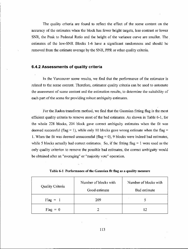
The quality criteria are found to reflect the effect of the scene content on the

accuracy of the estimates when the block has fewer bright targets, less contrast or lower

SNR, the Peak to Pedestal Ratio and the height of the variance curve are smaller. The

estimates of the low-SNR Blocks 1-6 have a significant randomness and should be

removed from the estimate average by the SNR, PPR or other quality criteria.

6.4.2 Assessments of quality criteria

In the Vancouver scene results, we find that the performance of the estimator is

related to the scene content. Therefore, estimator quality criteria can be used to automate

the assessment of scene content and the estimation results, to determine the suitability of

each part of the scene for providing robust ambiguity estimates.

For the Radon transform method, we find that the Gaussian fitting flag is the most

efficient quality criteria to remove most of the bad estimates. As shown in Table 6-1, for

the whole 228 blocks, 204 block gave correct ambiguity estimates when the fit was

deemed successful (flag =1), while only 10 blocks gave wrong estimate when the flag =

1. When the fit was deemed unsuccessful (flag = 0), 9 blocks were indeed bad estimates,

while 5 blocks actually had correct estimates. So, if the fitting flag = 1 were used as the

only quality criterion to remove the possible bad estimates, the correct ambiguity would

be obtained after an "averaging" or "majority vote" operation.

Table 6-1 Performance of the Gaussian fit flag as a quality measure

Quality Criteria Number of blocks with

Good estimate

Number of blocks with

Bad estimate

Flag = 1 209 5

Flag = 0 2 12

113

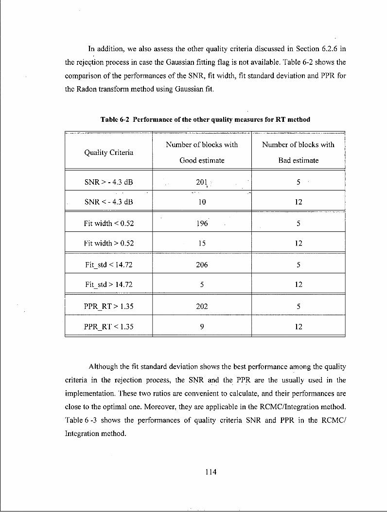
In addition, we also assess the other quality criteria discussed in Section 6.2.6 in

the rejection process in case the Gaussian fitting flag is not available. Table 6-2 shows the

comparison of the performances of the SNR, fit width, fit standard deviation and PPR for

the Radon transform method using Gaussian fit.

Table 6-2 Performance of the other quality measures for R T method

Quality Criteria Number of blocks with

Good estimate

Number of blocks with

Bad estimate

SNR > - 4.3 dB 201 ft

5

SNR < - 4.3 dB 10 12

Fit width < 0.52 196 5

Fit width > 0.52 15 12

Fit_std < 14.72 206 5

Fit_std> 14.72 5 12

PPR_RT> 1.35 202 5

PPR_RT< 1.35 9 12

Although the fit standard deviation shows the best performance among the quality

criteria in the rejection process, the SNR and the PPR are the usually used in the

implementation. These two ratios are convenient to calculate, and their performances are

close to the optimal one. Moreover, they are applicable in the RCMC/integration method.

Table 6 -3 shows the performances of quality criteria SNR and PPR in the RCMC/

Integration method.

114

Table 6-3 Performance of the quality measures for RCMC/integration method

Quality Criteria Number of blocks with

Good estimate

Number of blocks with

Bad estimate

SNR > - 4.3 dB 202 4

SNR < - 4.3 dB 10 12

PPR_RCin> 1.25 203 4

PPR_RCin< 1.25 9 12

6 .4 .3 Comparison of the experiment results

In this section, we examine and compare the performance of the Radon and

RCMC/integration estimators over a consistent set of blocks of the Vancouver scene.

Results of the standard MLCC and MLBF algorithms are included as well for

comparison. Each estimator has different quality measures, but in order to compare the

estimators fairly, we only use only one quality criterion in this comparison so that the

same blocks are rejected for each estimator. The quality criterion of "SNR > -1 dB" is

used, and 28 out of the 228 blocks are rejected. These are mainly the blocks that are

dominated by water areas.

Table 6-4 shows the comparison results of the performance of different estimators.

The second and the third column give the mean value and standard deviation of the

estimates before the rounding operation in the non-rejected blocks, while the final column

gives the percentage of the blocks with the correct estimates after rounding operation of

the non-rejected blocks. The first two rows assess the standard version of the MLCC and

MLBF algorithms described in Chapter 3. The next two rows give the results of the

iterative RCMC method and improved beat frequency estimation method described in

Chapter 4 and Chapter 5. The last three rows assess the Radon transform method using

115

the center of gravity measurement, the Radon transform method with Gaussian fit, and

finally the RCMC/integration method.

Table 6-4 Comparison of Doppler ambiguity resolvers for the Vancouver data

Doppler Ambiguity Resolvers Mean

(PRFs)

St. Dev.

(PRFs)

Success rate

(%)

Standard MLCC -5.83 1.36 41

Standard MLBF -5.72 1.09 62

MLBF using iterative RCMC -5.92 0.73 92

MLBF using ILP -5.89 0.43 85

Radon with Center of Gravity -5.99 0.16 99

Radon with Gaussian fit -5.98 0.14 99

RCMC with integration -6.01 0.10 99

The mean values of results are all close enough to the correct number for all

methods. However, the standard deviation is a more valuable assessment as it reveals the

degree of randomness directly. It can be seen that the estimates based on the Radon

transform and the RCMC/integration method are clearly giving estimates with less

variability. The Gaussian fit method of estimating the slope gives better results than the

center of gravity method, likely because it uses a more appropriate function in the fitting

procedure. Finally, the RCMC/integration method give equal or better results than the

Radon transform method, and may be the best one of all (note that the standard deviation

value for the RCMC/integration method is somewhat affected by the integer-quantized

solutions).

The histograms of the estimates of the different Doppler ambiguity resolvers

reveal the same comparison results as described above, as shown in Figure 6-13.

116

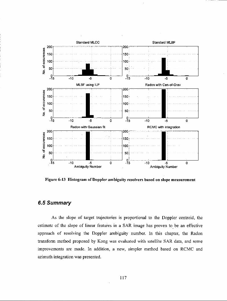
Standard MLCC Standard MLBF 200 F

0 -15

200 ;

rence

ren

ce

150 • O O 100 O

"o 50 6 z oL

-15

0 -15

-10 -5

MLBF using ILP

-10 -5

Radon with Gaussian fit

-10 -5 Ambiguity Number

200

•|150

100

50

0 -15

1200

150

1100

50

0 -15

200

150

100

50

0 -15

1. -10 -5

Radon with Cen-of-Grav

-10 -5

RCMC with integration

-10 -5 Ambiguity Number

Figure 6-13 Histogram of Doppler ambiguity resolvers based on slope measurement

6.5 Summary

As the slope of target trajectories is proportional to the Doppler centroid, the

estimate of the slope of linear features in a SAR image has proven to be an effective

approach of resolving the Doppler ambiguity number. In this chapter, the Radon

transform method proposed by Kong was evaluated with satellite SAR data, and some

improvements are made. In addition, a new, simpler method based on RCMC and

azimuth integration was presented.

117

Both the simulations and real data experiments show that the Doppler centroid

estimators based on slope measurement are effective in resolving the Doppler ambiguity

number. In the experiment using RADARSAT-1 data, the estimates can obtain an

unbiased Doppler Ambiguity number and have a much smaller standard deviation than

the current Doppler Ambiguity Estimators. It is shown that the slope estimation method

work well in medium to high contrast scenes, even when no prominent targets are visible.

The estimators gave correct result in almost all areas of the tested scene, except in calm

water.

118

Chapter 7

Conclusions

7.1 Summary

This thesis has focused on Doppler centroid estimation problems and

improvements to existing Doppler Ambiguity estimators for high-quality SAR

processing. We have presented several improvements to the existing MLBF and slope-

based estimation algorithms. In addition, experiments were conducted with the real

satellite dataset, RADARSAT-1 Vancouver scene, in order to test the performances of the

proposed methods.

Background to study

First, the Doppler centroid frequency and existing Doppler centroid estimation

algorithms were introduced. The "spectral fit" and ACCC algorithms were chosen as

reliable baseband Doppler estimators. The three phase-based Doppler ambiguity resolvers

(the WDA algorithm, MLCC algorithm, and MLBF algorithm) were discussed. The

WDA algorithm measures the slope of the centroid versus the transmission frequency

directly in the range frequency domain. The MLCC algorithm uses two range looks to

emulate two radars working in different transmission frequencies. The difference of the

central frequencies of the two looks is measured by using the ACCC calculation, and the

estimate of the absolute Doppler centroid is obtained. Like the MLCC algorithm, the

MLBF algorithm takes advantage of the two range looks to estimate the Doppler centroid.

These estimates can be obtained by beating the signals of the two looks and measuring

the beat frequency from the generated beat signal. Because of their different measurement

methods, the WDA and MLCC algorithm work well in low contrast scenes and can be

biased by partially exposed strong targets. On the other hand, the MLBF algorithm

119

performs well in high contrast scenes and does not suffer as much from partially exposed

bright targets as the other algorithms. In addition, the "spatial diversity" approach is used

to provide a single ambiguity number over the whole frame of data. Areas of the scene

that bias the estimates can be recognized using quality measures, and rejected from the

estimation process. Then, a polynomial or geometry model can be used to fit a Doppler

surface over the whole frame.

Principle of the MLBF algorithm

Since the MLBF algorithm proves to be one of the most reliable ways of

estimating the Doppler centroid frequency of SAR signals, we mainly concentrated on

this popular algorithm. We discussed a number of ways of improving its estimation

sensitivity. First, we examined the principle of the MLBF algorithm in more detail, and

gave a more thorough, frequency domain explanation of how it works. We showed how

the phase of each range look depends on the range migration and how the phase varies in

the range frequency domain. Based on this analysis, we highlighted the importance of

extracting symmetrical range looks and shifting the range looks to baseband.

The benefits of applying RCMC

We also found that the RCMC has the effect of narrowing the bandwidth of the

beat signal, and reducing the effect of cross beating when more than one significant target

is present in one range cell. The noise in the beat signal due to cross beating is thereby

reduced, allowing the FFT to obtain finer resolution because of the longer target exposure

time in each range cell. Therefore, we considered using the RCMC to straighten the target

trajectories before the beat frequency estimator is applied. We also demonstrated that the

RCMC must be applied after the look extraction to preserve the phase variation, a point

that was not obvious when the problem was first considered. If the RCMC is applied

before the look extraction, the beat signal would have constant phase and the Doppler

centroid could not be obtained from the measurement of the beat frequency. Based on the

above analysis, we proposed an iterative scheme.of.applying the RCMC, since the

ambiguity number is needed to be updated for correct RCMC.

120

Improved frequency estimator The existing MLBF algorithm uses FFT operations to estimate the beat frequency

by finding the maximum coefficient. This method has limitations of resolution and

quantization, especially when the signal is discontinuous in one range cell due to range

cell migration or burst mode operation. We thereby considered using more accurate

frequency estimation methods based on phase increments and noise rejection filters to

improve the beat frequency estimation. In this thesis, we examined five established

frequency estimators, including Kay's estimator, the ACCC estimator, the FCFB

estimator, the HLC estimator, and the ILP estimator. We discussed the processing

procedures of all the estimators and the quality measurements of the phase coherence,

which especially for the estimator using phase increments. Since the ILP estimator is the

most accurate frequency estimator in the literature, we replaced the conventional FFT

estimator with the ILP estimator to improve the beat frequency estimation. Although this

method and the iterative RCMC algorithm can be combined, the majority of the

estimation improvement can be obtained by using one of the modifications alone, as each

method approaches the same sensitivity problem in a different fashion.

Improved slope estimation algorithm

We also examined and improved the methods that estimate the Doppler centroid

by measuring the alignment of linear features in SAR data. These methods are based on

the same principle as the "look misregistration" algorithm. The slope estimation methods

take advantage of the fact that Range Migration is caused by the beam squint angle and its

slope is proportional to the Doppler centroid. Kong has proposed a method that uses the

Radon transform to measure the slope of the target energy and obtain the absolute

Doppler centroid for the airborne SAR data. In our study, we discussed the properties

and application of the Radon transform in more detail, and examined Kong's method in

the Doppler ambiguity resolution for satellite SAR data. We developed an alternative and

computationally simpler method that uses RCMC with azimuth integration in Doppler

ambiguity resolution. This method employs the RCMC to change the slope of targets

trajectories, and uses azimuth integration to find which Doppler ambiguity number makes

the trajectories vertical. Several quality measurements of the "spatial diversity" approach

121

derived from the data and from each particular estimator were used to increase the

robustness of the algorithm.

Experiments with RADARSAT data

The experiments with RADARSAT-1 data showed that the improved method

yields more consistent estimates than does the existing algorithms. The proposed iterative

RCMC method can increase the percentage of blocks yielding the correct ambiguity

number from 62 to 92%. The method using the ILP estimator can obtain a standard

deviation less than half that obtained by the existing method, and a much higher

percentage of blocks that yield the correct ambiguity number. In addition, the slope

estimation methods work well in medium to high contrast scenes, even when no

prominent targets are visible. They can significantly increase the percentage of blocks

yielding the correct ambiguity number. The improved estimators work best with the high

contrast scenes, but work surprisingly well in medium to low contrast scenes.

7.2 Contributions

This thesis has presented several improved techniques for estimating the Doppler

centroid in satellite SAR data. Particularly, we have:

• proposed a method that applies the RCMC after look extraction to reduce cross-

beating and narrow the bandwidth of the beat signal, thereby improving the

estimate results of the MLBF algorithm;

• proposed a method that uses more accurate frequency estimators based on phase

increments to improve estimation of the beat frequency, which thereby improves

the performance of the existing MLBF algorithm;

• applied the method using the Radon transform in the Doppler ambiguity

resolution for satellite SAR data, and proposed some minor improvements to this

method;

122

• proposed a simpler slope measurement method for Doppler ambiguity resolution

using RCMC and azimuth integration, which has the same or even better

performance than Kong's method; and

• developed several quality measurements for the proposed methods and

implemented them in the "spatial selected" approach.

7.3 Future Work

The results of our research suggest the following topics for future investigation:

• The improved MLBF algorithms and the improved slope estimation algorithms

can be combined together to further increase the sensitivity of estimate results.

• Better quality measurements need to be developed to remove more bad estimates

and increase the robustness of the Doppler ambiguity resolvers.

• More real datasets with different contents should be used to test the performance

of the proposed algorithms, such as ENVISAT data.

• The proposed algorithms should be applied to ScanSAR data to test their

performance with burst mode datasets.

123

Bibliography

[1] J. J. Kovaly, "Synthetic Aperture Radar," Artech House, Dedham, MA, 1976.

[2] I. G. Cumming and J. R. Bennett, "Digital Processing of SEASAR SAR Data," in

Rec. IEEE International Conference on Acoustics, Speech and Signal Processing,

pp. 710-718, Aprirl 1979.

[3] C. Wu, K. Y. Liu, and M. J. Jin, "A Modeling and Correlation Algorithm for

Spaceborne SAR Signals," IEEE Trans, on Aerospace and Electronic Systems,

Vol. 18, Issue 5, pp. 563-574, September 1982.

[4] R. K. Raney, H. Runge, R. Bamler, I. G. Cumming, and F. H. Wong, "Precision

SAR Processing Using Chirp Scaling," IEEE Trans. Geoscience and Remote

Sensing, Vol. 32, Issue 4, pp. 786-799, July 1994.

[5] A. A. Thompson, J. C. Curlander, N. S. Mclagan, T. E. Feather, M. D'lorio, and J.

Lam, "ScanSAR Processing Using the Fast Scan System," in Proceedings of the

International Geoscience and Remote Sensing Symp., IGARSS'94, Vol. 2, pp.

1187-1189, August 1994.

[6] H. Ffellsten and L. E. Anderson, "An Inverse Method for the Processing of

Synthetic Aperture Radar Data," Inverse Problems, Vol. 3, Issue 1, pp. 111-124,

February 1987.

[7] F. K. Li, D. H. Held, J. C. Curlander, and C. Wu, "Doppler Parameter Estimation

for Spaceborne Synthetic Aperture Radars," IEEE Trans. Geoscience and Remote

Sensing, Vol. 23, Issue 1, pp. 47-56, January 1985.

[8] S. N. Madsen, "Estimating the Doppler Centroid of SAR Data," IEEE Trans.

Aerospace Electronic system, Vol. 25, Issue 2, pp. 134-140, March 1989.

[9] R. Bamler, "Doppler Fequency Estimation and Cramer-Rao Bound," IEEE Trans.

Geoscience and Remote Sensing, Vol. 29, Issue 3, pp. 385-390, May 1991.

[10] I. G. Cumming, P. F. Kavanagh, and M. R. Ito, "Resolving the Doppler

Ambiguity for Spaceborne Synthetic Aperture Radar," in Proceedings of the

124

International Geoscience and Remote Sensing Symposium, IGARSS'86, pp. 1639-

1643, September 1986.

[11] C. Y. Chang and J. C. Curlander, "Application of the Multiple PRF Technique to

Resolve Doppler Centroid Estimation Ambiguity for Spaceborne SAR," IEEE

Trans. Geoscience and Remote Sensing, Vol. 30, pp. 941-949, September 1992.

[12] R. Bamler and H. Runge, "PRF-ambiguity Resolving by Wavelength Diversity,"

IEEE Trans. Geoscience and Remote Sensing, Vol. 29, pp. 997-1003, November

1991.

[13] F. H. Wong and I. G. Cumming, "A Combined SAR Doppler Centroid Estimation

Scheme Based upon Signal Phase," IEEE Trans, on Geoscience and Remote

Sensing, Vol. 34, pp. 696-707, May 1996.

[14] J. Curlander and R. McDonough, "Synthetic Aperture Radar: Systems and Signal

Processing," John Wiley & Sons, New York, November 1991.

[15] I. G- Cumming and F. H. Wong, "Digital Processing of Synthetic Aperture Radar

Data Algorithms and Implementation," Artech House, Norwood, MA, January

2005.

[16] Tonghua Zhang, "Investigation of Biases in Doppler Centroid Estimation

Algorithms," Master's thesis, Dept. of Electrical and Computer Engineering, The

University of British Columbia, August 1999.

[17] R. K. Hawkins, T. I. Lukowski, K. P. Murnaghan, and S. K. Srivastava, "The

Effects of Doppler Processing Errors in SAR Data," in Proceedings of the CEOS

SAR Calibration Workshop, pp. 201-208, February 1998.

[18] I. G. Cumming, "Model-Based Doppler Estimation for Frame-Based SAR

Processing," in Proceedings of International Geoscience and Remote Sensing

Symp., IGARSS'01, Vol. 6, pp. 2645-2647, July 2001.

[19] I. G. Cumming. "A Spatially Selective Approach to Doppler Estimation for

Frame-Based Satellite SAR Processing," IEEE Trans, on Geoscience and Remote

Sensing, Vol. 42, Issue 6, pp. 1135-1148, June 2004.

[20] Stability and Controllability, Flight Training Handbook, AvStop Magazine online

from: http://avstop.com/AC/FlightTraingHandbook/Stability.html

125

[21] M. Y. Jin, "Optimal Doppler Centroid Estimation for SAR Data From A Quasi-

homogeneous Source," IEEE Trans. Geoscience and Remote Sensing, Vol. GE-

24, pp. 1022-1025, March 1986.

[22] C. Cafforio, P. Guccione, and A. Monti Guarnieri, "Doppler Centroid Estimation

for ScanSAR Data," IEEE Trans, on Geoscience and Remote Sensing, Vol. 42,

Issue 1, pp. 14-23, January 2004.

[23] M. V. Dragosevic and B. Plache, "Doppler Tracker for A Spaceborne ScanSAR

System," IEEE Trans. Aerospace Electroic. System, Vol. 36, pp. 907-924, July

2000.

[24] E. O. Brigham, "The Fast Fourier Transform: An Introduction to Its Theory and

Application," Prentice Hall, Upper Saddle River, NJ, November 1973.

[25] Discussions with Dr. Ian Cumming, March 2005.

[26] Personal communication with Dr. Frank Wong and Dr. Ian Cumming, May 2005.

[27] D. Rife and R. Boorstyn, "Single-tone Parameter Estimation from Discrete-time

Observations," IEEE Trans. Inform. Theory, Vol. IT-20, pp.591-598, September

1974.

[28] S. Kay, "Modern Spectral Estimation: Theory and Application," Englewood Cliffs.

NJ: Prentice-Hall, 1988.

[29] A. Herment, G. Demoment. P. Dumee, J. P. Guglielmi, and A. Delouche, "A New

Adaptive Mean Frequency Estiamtor: Application to Constant Variance Color

Flow Mapping," IEEE Trans, on Ultrasonics, Ferroeletrics, and Frequency

Control, Vol. 40, Issue 6, pp. 796-804 , November 1993.

[30] S. Kay, "A Fast and Accurate Single Frequency Estimator," IEEE Trans.

Acoustic, Speech, Signal Processing, Vol. 37, pp. 1987-1990. December 1989.

[31] M. Fowler and J. Johnson, "Extending the Threshold and Frequency Range for

Phase-based Frequency Estimation," IEEE Trans. Signal Processing, Vol. 47, pp.

2857-2863, October 1999.

[32] M. P. Fitz, "Further Results in the Fast Estimation of A Single Frequency," IEEE

Trans, on Communication, Vol. 42, Part 2. pp. 862-864, February-April 1994.

126

[33] T. Brown and M. M. Wang, "An Iterative Algorithm for Single-frequency

Estimation," IEEE Trans. Signal Processing, Vol. 50, No. 11, pp. 2671-2682,

November 2002.

[34] S. Li and I. G. Cumming, "Improved Beat Frequency Estimation in the MLBF

Doppler Ambiguity Resolver," in IEEE Proceedings of International Geoscience

and Remote Sensing Symp., IGARSS'05, Vol. 5, pp. 3348-3351, July 2005.

[35] Y.-K. Kong, B.-L. Cho, and Y.-S. Kim, "Ambiguity-Free Doppler Centroid

Estimation Technique for Airborne SAR Using the Radon Transform," IEEE

Trans. Geoscience and Remote Sensing, Vol. 43, Issue 4, pp. 715-721, April 2005.

[36] P. Toft, "The Radon Transform - Theory and Implementation," PhD Thesis,

Informatics and Mathematical Modeling, Technical University of Demark, 1996

[37] A. L. Warrick and P. A. Delaney, "Detection of Linear Features Using a Localized

Radon Transform," in Conference Record of the Thirtieth Asilomar Conference on

Signals, Systems and Computers, Vol. 2, pp. 1245 - 1249, November 1996.

[38] A. C. Copeland, G. Ravichandran, and M. M. Trivedi, "Localized Radon

Transform-based Detection of Ship Wakes in SAR Images," IEEE Trans, on

Geoscience and Remote Sensing, Vol. 33, pp. 35-45, January 1995.

[39] J. A. Nelder and R. Mead, "A Simplex Method for Function Minimization,"

Computer Journal, Vol. 7, pp. 308-313, 1965. Available in MATLAB as the

function FMINSEARCH.

127