Improved Birnbaum–Saunders inference under type II censoring

Computational Statistics and Data Analysis 57 (2013) 68–81

Contents lists available at SciVerse ScienceDirect

Computational Statistics and Data Analysis

journal homepage: www.elsevier.com/locate/csda

Improved Birnbaum–Saunders inference under type II censoringLarissa Santana Barreto, Audrey H.M.A. Cysneiros ∗, Francisco Cribari-NetoDepartamento de Estatística, Universidade Federal de Pernambuco, Cidade Universitária, Recife/PE, 50740–540, Brazil

a r t i c l e i n f o

Article history:Received 28 August 2011Received in revised form 2 April 2012Accepted 5 June 2012Available online 16 June 2012

Keywords:BiasBirnbaum–Saunders distributionBootstrapLikelihood ratio testMaximum likelihood estimationModified profile likelihood

a b s t r a c t

The Birnbaum–Saunders distribution is useful for modeling reliability data. In this paperwe obtain adjusted profile maximum likelihood estimators for the Birnbaum–Saundersdistribution shape parameter under type II data censoring. We consider the adjustmentsto the profile likelihood function proposed by Barndorff-Nielsen (1983), Cox and Reid(1987), Fraser and Reid (1995), Fraser et al. (1999) and Severini (1998, 1999). We obtainmodified profile likelihood ratio tests and also consider bootstrap-based inference. Intervalestimation is addressed as well. Several bootstrap confidence intervals are considered.Monte Carlo simulation results on point estimation, interval estimation and hypothesistesting inference are reported. Finally, we present two applications that use real (notsimulated) data.

© 2012 Elsevier B.V. All rights reserved.

1. Introduction

Practitioners often analyze data on the time elapsed until a certain event takes place. Several models have beenconsidered for analyzing such data. Birnbaum and Saunders (1969a) introduced a two-parameter distribution for modelinglifetime data using amodel in which failure follows from the development and growth of a dominant crack. The distributionwas later derived by Desmond (1985) under less stringent assumptions. He also investigated the relationship betweenthe Birnbaum–Saunders and inverse Gaussian distributions (Desmond, 1986). The Birnbaum–Saunders distribution hasthe appealing feature of typically providing satisfactory tail fitting and has been widely revisited in the last decade or so;see, e.g., Cysneiros et al. (2008), Díaz-Garcia and Leiva-Sánchez (2005), Galea et al. (2004), Lemonte et al. (2007), Ng et al.(2003, 2006), Wang et al. (2006) and Wu and Wong (1994). In particular, Cysneiros et al. (2008) develop a modified profilelikelihood estimation (point estimation and hypothesis testing) under complete data (no censoring). It is common, however,for lifetime data to be subject to censoring. Our chief goal in this paper is to extend their results to situations in which thedata are collected under type II censoring and to also consider interval estimation. We obtain adjustments to the profilelikelihood function that deliver more accurate inference on the Birnbaum–Saunders shape parameter. Different modifiedlikelihood ratio tests are presented. Inference based on such tests is typically more reliable than that based on the standardlikelihood ratio test, as evidenced by our numerical (Monte Carlo) results. We also consider hypothesis testing inferenceunder data resampling. To that end, a bootstrapping scheme is employed to estimate the test statistic null distributionand the corresponding inference is based on the comparison between the test statistic and a critical value obtained from theestimated null distribution. Practitioners are usually also interested in performing interval estimation.We consider the usualasymptotic confidence interval, which is obtained from the asymptotic normality of themaximum likelihood estimator, andalso different bootstrap-based confidence intervals. As revealed by our numerical results, bootstrap interval estimation canlead to much more accurate inferences in small samples than the standard approximate confidence interval.

∗ Corresponding author. Tel.: +55 8121267435; fax: +55 8121268422.E-mail addresses: [email protected] (L.S. Barreto), [email protected] (A.H.M.A. Cysneiros), [email protected] (F. Cribari-Neto).URLs: http://www.de.ufpe.br/∼audrey (A.H.M.A. Cysneiros), http://www.de.ufpe.br/∼cribari (F. Cribari-Neto).

0167-9473/$ – see front matter© 2012 Elsevier B.V. All rights reserved.doi:10.1016/j.csda.2012.06.005

L.S. Barreto et al. / Computational Statistics and Data Analysis 57 (2013) 68–81 69

The paper unfolds as follows. Section 2 describes different adjustments to profile likelihood functions. In Section 3 weobtain adjustments to the Birnbaum–Saunders log-likelihood function and describe bootstrap-based inference. Numerical(Monte Carlo) results on point estimation, interval estimation and hypothesis testing inference are presented and discussedin Sections 4 and 5. Two applications that use real (not simulated) data are presented in Section 6. Finally, Section 7 offerssome concluding remarks.

2. Adjustments to the profile likelihood function

Let θ = (τ⊤, φ⊤)⊤ be the parameter vector that indexes a statistical model and assume that τ and φ are the interestand nuisance parameters, respectively. Also, let L(τ , φ) denote the corresponding likelihood function which is constructedusing a sample of n observations. The profile likelihood function for τ is defined as

Lp(τ ) = L(τ ,φτ ),

where L(·) is the usual likelihood function andφτ is the maximum likelihood estimator of φ for a given value of τ .Since the profile likelihood function is obtained by replacing the nuisance parameter φ by an estimate, φτ , it is not a

genuine likelihood function, i.e., it does not have all of the desirable properties that a true likelihood function enjoys. Forinstance, there exist both score and information biases, which are of order O(1). Note that by fixing the nuisance parameterat its point estimate one to some extent neglects the uncertainty involved in such estimation. It should be noted, however,that the likelihood ratio statistic based on the profile log-likelihood function ℓp(τ ) for making inference on the parameter ofinterest equals that based on the log-likelihood function ℓ(τ , φ), that is, LR = 2

ℓ(τ ,φ) − ℓ(τ ,φτ )

= 2

ℓp(τ) − ℓp(τ )

,

whereτ andφ are, respectively, the maximum likelihood estimators of τ and φ.Several modifications of the profile likelihood function were proposed in the literature. They all aim at reducing the

impact of the nuisance parameter on inferences made about the parameter of interest. Barndorff-Nielsen (1983) obtaineda modified profile likelihood function which is an approximation to the marginal or conditional likelihood function for τ , ifeither exists. His proposal follows from the p∗ formula,which is an approximation to the conditional density of themaximumlikelihood estimator given an ancillary statistic. His modified log-likelihood function can be expressed as

ℓBN(τ ) = ℓp(τ ) − log∂φτ

∂φ− 1

2log |jφφ(τ ,φτ ;τ ,φ, a)|, (2.1)

where jφφ(τ ,φτ ;τ ,φ, a) = −∂2ℓ(τ ,φ;τ ,φ,a)

∂φ2 (notice that it is evaluated at (τ ,φτ )) and∂φτ

∂φ is the matrix of partial derivatives

ofφτ with respect toφ. The maximizer of ℓBN(τ ) is denoted byτBN.An alternative expression for the log-likelihood function in (2.1) follows from replacing ∂φτ/∂φ by jφφ(τ ,φτ ;τ ,φ, a)−1

ℓφ;φ(τ ,φτ ;τ ,φ, a):

ℓBN(τ ) = ℓp(τ ) +12log |jφφ(τ ,φτ ;τ ,φ, a)| − log |ℓφ;φ(τ ,φτ ;τ ,φ, a)|,

where

ℓφ;φ(τ , φτ ; τ , φ, a) =∂

∂φ

∂ℓ(τ , φτ ; τ , φ, a)

∂φ

.

Note, however, that the latter form involves a sample space derivative and requires an ancillary statistic a such that (τ ,φ, a)is minimally sufficient.

Some approximations to the abovemodified log-likelihood functionwere proposed. They follow from approximating thesample space derivative. Severini’s (1999) approximation can be easily computed and has an error of order O(n−1/2). It isparticularly useful when expected values of products of log-likelihood derivatives are hard to obtain. His approximation isgiven by

ℓBN(τ ) = ℓp(τ ) +12log |jφφ(τ ,φτ )| − log |Iφ(τ ,φτ ;τ ,φ)|,

where

Iφ(τ , φ; τ0, φ0) =

nj=1

ℓ(j)φ (τ , φ)ℓ

(j)φ (τ0, φ0)

⊤.

Here, ℓ(j)φ is the score function for the jth observation. We denote the corresponding maximum likelihood estimator by τ BN.

A second approximation to Barndorff-Nielsen’s modified profile likelihood function was introduced by Fraser and Reid(1995) and by Fraser et al. (1999). It is given by

ℓBN(τ ) = ℓp(τ ) +12log |jφφ(φτ , τ )| − log |ℓφ;T (φτ , τ )Vφ |, (2.2)

70 L.S. Barreto et al. / Computational Statistics and Data Analysis 57 (2013) 68–81

where ℓφ;T (φ, τ ) = ∂ℓφ(φ, τ )/∂T ′, ℓφ(φ, τ ) being the score function for φ, T ′= (t1, . . . , tn) and

Vφ =

−

∂F(y1;φ,τ)/∂φf (y1;φ,τ)

, . . . ,−∂F(yn;φ,τ)/∂φ

f (yn;φ,τ)

′

.

The corresponding maximum likelihood estimator is denoted by τ BN.Cox and Reid (1987) obtained a modified profile log-likelihood function that approximates the conditional density

function of the observations given the nuisance parameter. It is given by

ℓCR(τ ) = ℓp(τ ) −12log |jφφ(τ ,φτ )|.

Like ℓBN(τ ), the above function is a penalized profile log-likelihood function. Here, however, the interest and nuisanceparameters must be orthogonal. We note that the Cox and Reid (1987) log-likelihood function is invariant underreparameterizations of the form (τ , φ) → (τ , ζ (τ , φ)) and we denote the maximizer of ℓCR(τ ) byτCR.

For further details on adjustments to the profile likelihood function, we refer readers to Pace and Salvan (1997) andSeverini (2000).

3. Improved Birnbaum–Saunders inference under type II censoring

Let {t(1), . . . , t(r)} be the r smallest observations of an independent sample of size n from a Birnbaum–Saundersdistributed random variable T . We say that {t(1), . . . , t(r), t(r), . . . , t(r)} is a sample of size n subject to type II censoring,where n − r observations are censored. The likelihood function is given by

L = L(α, β) =n!

(n − r)!

1 − Φ

1α

ξ

t(r)β

n−r

1√2παβ

r

ri=1

ξ ′

t(i)β

exp

−

12α2

ri=1

ξ 2t(i)β

and the log-likelihood function is

ℓ = log(L) = c + (n − r) log1 − Φ

1α

ξ

t(r)β

− r log(αβ) +

ri=1

logξ ′

t(i)β

−

12α2

ri=1

ξ 2t(i)β

,

where c = log

n!(n−r)!

−

r2 log(2π), ξ(z) = z1/2 − z−1/2 and ξ ′(z) = (z1/2 + z−1/2)/(2z).

In what follows we shall use the following notation:

t∗(i) =t(i)β

, u∗=

1r

ri=1

t∗(i), v∗=

1r

ri=1

1t∗(i)

−1

,

K ∗(β) =

1r

ri=1

11 + t∗(i)

−1

and H(x) =φ(x)

1 − Φ(x).

Note that H(x) is the standard normal (Gaussian) risk function.The restricted maximum likelihood estimator of β , sayβα , is obtained from the following nonlinear equation:

Q (β) = ϕ2(β)

12

−1

K ∗(β)

−

u∗

2+

12v∗

−ϕ(β)(n − r)

r× H

1

ϕ(β)ξ(t∗(r))

t∗(r)ξ

′(t∗(r)), (3.1)

where ϕ2(β) = α2= (h2(β)h3(β) − h1(β)h4(β))/(h1(β) − h3(β)). Here,

h1(β) = ξ(t∗(r)),

h2(β) = −1r

ri=1

ξ 2(t∗(i)),

h3(β) =

1 +

1r

ri=1

t∗(i)ξ′′(t∗(i))

ξ ′(t∗(i))

−1

t∗(r)ξ′(t∗(r)),

h4(β) =

1 +

1r

ri=1

t∗(i)ξ′′(t∗(i))

ξ ′(t∗(i))

−1 −

1r

ri=1

t∗(i)ξ(t∗(i))ξ′(t∗(i))

.

See Ng et al. (2006) for details. We note that the restricted maximum likelihood estimator of β equals the correspondingstandard maximum likelihood estimator, that is,βα = β .

L.S. Barreto et al. / Computational Statistics and Data Analysis 57 (2013) 68–81 71

It follows from the definition of the profile likelihood function that

ℓp(α) = (n − r) log1 − Φ

1α

ξ

t(r)βα

− r log(αβα) +

ri=1

logξ ′

t(i)βα

−

12α2

ri=1

ξ 2t(i)βα

.

The profile maximum likelihood estimator of α – the maximizer of ℓp(α) – is denoted byαp.We shall now obtain adjustments to the Birnbaum–Saunders profile likelihood function using the results outlined in

Section 2.At the outset, we obtain two approximations to Barndorff-Nielsen’s (1983)modified profile log-likelihood function. They

use the approximations to the sample space derivative proposed by Severini (1999) and Fraser and Reid (1995) and are given,respectively, by

ℓBN(α) = ℓp(α) +12log |jββ(α,βα)| − log |Iβ(α,βα;α,β)| (3.2)

and

ℓBN(α) = ℓp(α) +12log |jββ(α,βα)| − log |ℓβ;T (α,βα)Vβ |, (3.3)

where

Iβ(α,βα;α,β) =

rj=1

1β2

12

−

βt(j) +β −

12α2

t(j)β −

βt(j)

12

−

βt(j) +β −

12α2

t(j)β −

βt(j)

+ (n − r)H

1α

ξ

t(r)β

H1α ξ

t(r)β

1

ααβ2

ξ ′

t(r)β2 t(r)β

2

,

ℓβ;T (α,βα)Vβ =

r−1i=1

t(i)β

−1

t(i) +βα

+1

2(αβα)2+

12(t(i)α)2

+ (n − r + 1)

t(r)β×

(n − r)

αβα

1βα

H1α

ξ(t∗(r))

t∗(r)ξ′′(t∗(r)) + ξ ′(t∗(r))

+

t∗(r)αβα

ξ ′(t∗(r))

2 H ′

1α

ξ(t∗(r))

+ (n − r + 1)t(r)β

−

1

(t(r) +βα)2+

1

2(αβα)2+

12(t(r)α)2

and

jββ(α,βα) =r

(αβα)2

−Q (βα) + A31

. (3.4)

In order to solve Eq. (3.4) we use Eq. (3.1) evaluated atβα together with

H ′(x) = −xH(x) + H2(x)

and

A31 = −α2

1K ∗

−1r

ri=1

1(1 + t∗(i))2

+

u∗

2+

12v∗

+α(n − r)

rt∗(r)

×

H1α

ξ(t∗(r))

t∗(r)ξ′′(t∗(r)) + ξ ′(t∗(r))

+

t∗(r)α

ξ ′(t∗(r))

2 H ′

1α

ξ(t∗(r))

.

We denote the adjusted profile maximum likelihood estimators of α obtained from (3.2) and (3.3) by αBN and αBN,respectively.

It can be shown that Cox and Reid’s (1987) modified Birnbaum–Saunders log-likelihood function can be expressed as

ℓCR(α) = ℓp(α) −12log |jββ(α,βα)|,

where jββ is as given in (3.4). The corresponding adjusted profile maximum likelihood estimator of α is denoted byαCR.The estimators βα,αp, αBN,αBN, αCR do not have closed-form. They can be computed by numerically maximizing the

corresponding log-likelihood function using, e.g., a Newton or quasi-Newton algorithm; see Nocedal and Wright (1999).Suppose now that the interest lies in testing the null hypothesis H0 : α = α0 against the alternative hypothesis

H1 : α = α0, where α0 is a given scalar. The profile and adjusted profile likelihood ratio test statistics are given by

LRp = 2ℓp(αp) − ℓp(α0)

,

LRBN−1 = 2ℓBN(α) − ℓBN(α0)

,

LRBN−2 = 2ℓBN(α) − ℓBN(α0)

72 L.S. Barreto et al. / Computational Statistics and Data Analysis 57 (2013) 68–81

and

LRCR = 2 {ℓCR(αCR) − ℓCR(α0)} .

Under the null hypothesis, they are all asymptotically distributed as χ21 .

It is noteworthy that, as pointed out in Section 2, the Cox and Reid (1987) adjustment to the profile likelihood functionrequires orthogonality between the parameter of interest and the nuisance parameter. Under complete data, the parametersthat index the Birnbaum–Saunders distribution are orthogonal, i.e., the off-diagonal elements of Fisher’s informationmatrixare equal to zero; see Lemonte et al. (2007). Under type II censoring, however, Fisher’s informationmatrix cannot be obtainedanalytically.We are thus unsure of the orthogonality betweenα andβ .We shall, however,workwith the Cox andReid (1987)adjustment. Our numerical (Monte Carlo) results show that it typically delivers reliable inference.

An alternative approach involves the estimation of the test statistic null distribution using data resampling. Morespecifically, B pseudo-samples of size n are generated from the Birnbaum–Saunders distribution after replacing α and βby α0 and β , respectively. Observations are censored according to the type II censoring in the original sample. Note thatthe data resampling is performed by imposing the null hypothesis. The test statistic is computed for each artificial sample.The critical value to be used in the test is then obtained as the 1 − γ quantile of the B test statistics computed from thepseudo-samples, where γ is the nominal level of the test. The null hypothesis is rejected if LRp exceeds the critical valueestimated from the B artificial samples. This sampling scheme is known as parametric bootstrap (Efron, 1979).

Practitioners are also usually interested in performing interval estimation. The usual approach is to employ an asymptoticconfidence interval (ACI) which follows from the asymptotic distribution of the maximum likelihood estimators. When thesample size is large, the maximum likelihood estimatorsα andβ are approximately normally distributed:αβ

A∼ N2

αβ

,

V11 V12V21 V22

,

whereV11 V12V21 V22

= V is theinverse of Fisher’s information. We then have the following asymptotic 100(1− γ )% (0 < γ <

1/2) confidence interval for α:α + zγ /2

V11,α + z1−γ /2

V11

,

where zp is such that Pr(Z ≤ zp) = p, Z ∼ N (0, 1) and hats denote evaluation at the maximum likelihood estimates. Here,zp denotes the pth (0 < p < 1) standardnormal quantile. Inwhat follows,V11 is the (1, 1) element of the observed informationmatrix evaluated at the maximum likelihood estimators, since no closed-form expression for Fisher’s information matrixis available under type II censoring. It is noteworthy that such an interval is based on a large sample approximation andmay be inaccurate in small samples. We also note that it may include negative values with positive probability and that itis always symmetric.

An alternative lies in the use of bootstrap resampling. Different bootstrap-based confidence intervals can be constructed.The percentile bootstrap confidence interval for α is obtained from the empirical distribution ofα, which is constructedusing B bootstrap (censored) samples. We generate B (censored) bootstrap samples (parametric bootstrap) and computeα∗b for each pseudo-sample (b = 1, . . . , B), i.e., we estimate the parameter α using each of the artificial datasets. The Bestimates are then ordered and we take the bootstrap estimates at the B × (γ /2) and B × (1 − γ /2) positions as the lowerand upper limits of the (1 − γ ) × 100% confidence interval, 0 < γ < 1/2. We denote these quantities as α∗(γ /2) andα∗(1−γ /2), respectively. If B× (γ /2) and B× (1−γ /2) are not integers, we can proceed as follows. Let k = ⌊(B + 1) × γ /2⌋(the greatest integer that does not exceed (B + 1) × γ /2), and use as lower and upper interval limits the k and (B + 1 − k)bootstrap replicates, respectively. The percentile confidence interval for α is thus given byα∗(γ /2),α∗(1−γ /2) .

The bootstrap-t confidence interval with coverage (1−γ )×100% can be computed as follows.We generate B (censored)bootstrap samples and for each sample we compute the statistic T ∗b

= (α∗b−α)/ep∗b, whereα is the estimate computed

using the original sample, α∗b is the estimate from the bth pseudo-sample and ep∗b is the standard error of α∗b (b =

1, . . . , B), which is obtained from the inverse of the observed information matrix. Let t(γ /2) and t(1−γ /2) be the bootstrapreplicates at positions B × (γ /2) and B × (1 − γ /2), respectively, after all bootstrap values are ordered. If B × (γ /2) andB×(1−γ /2) are not integers,we proceed as outlined in the description of the percentile confidence interval. The bootstrap-tconfidence interval isα − t(1−γ /2)ep,α − t(γ /2)ep .

Another bootstrap confidence interval is the BCa interval. In order to construct the BCa interval with (1 − γ ) × 100%coverage we obtain B bootstrap samples from the original sample and compute α∗b for each pseudo-dataset. We thencompute the following quantities:

v0 = Φ−1#{α∗b <α}

B

,

L.S. Barreto et al. / Computational Statistics and Data Analysis 57 (2013) 68–81 73

a =16Skew(uα(α)),

δ1 = Φ

v0 +v0 + zγ /2

1 −a(v0 + zγ /2)

,

δ2 = Φ

v0 +v0 + z1−γ /2

1 −a(v0 + z1−γ /2)

,

where Skew(·) denotes the skewness coefficient and uα is the log-likelihood derivative with respect to α evaluated atα. Weorder the B bootstrap values ofα∗b and take as lower and upper confidence intervals limits the B× δ1 and B× δ2 replicates.The BCa confidence interval is thus given byα∗(δ1),α∗(δ2)

.

In all bootstrapping schemes used for interval estimation, sampling is to be performed parametrically. That is, wemust sample from the Birnbaum–Saunders distribution after replacing the parameters that index the distribution by theircorresponding estimates (computed from the original data). We also note that the bootstrap samples should be censoredfollowing the original sample censoring, i.e., they should include the same number of censored observations as the originalsample. For further details on bootstrap inference, we refer readers to Davison and Hinkley (1997).

4. Monte Carlo simulation results

In what follows we shall report Monte Carlo simulation results on point estimation, interval estimation and hypothesistesting inference. The parameter of interest is α. For point estimation and hypothesis testing inference, we base ourresults on 10,000 Monte Carlo replications and B = 600 bootstrap replications. For interval estimation, the number ofbootstrap replications is increased to B = 1000. The sample sizes are n = 20 and n = 30, the values of the parameterof interest are α = 0.10, 0.25, 0.50, 1.00, the value of β is fixed at 1.00 and censoring covers 10%, 30% and 50% of allobservations. All simulations were carried out using the Ox matrix programming language (Doornik, 2009) and all log-likelihood maximizations were performed using the BFGS quasi-Newton algorithm. Bootstrap sampling was performedparametrically.

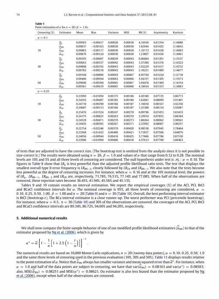
Tables 1–4 contain simulation results on point estimation.We report themean, bias, variance,mean squared error (MSE),relative bias (RB), asymmetry and kurtosis of the following estimators:αp,αBN, αBN andαCR. We note, at the outset, thatthe adjusted profile maximum likelihood estimators display smaller relative biases than the standard maximum likelihoodestimator (αp), the best performing estimator being αBN. For instance, in Table 2 with α = 0.50 and 10% censoring, therelative biases are 1.16% (αBN), 1.28% (αCR), 1.63% (αBN) and 4.30% (αp). The relative bias of the standardmaximum likelihoodestimator is thus nearly four times larger than that of the best performing modified estimator. Second, the relative biasesincrease with the proportion of censored observations. For example, we notice from Table 2 (α = 0.5) that when thepercentage of censored observations equals 30% and 50% the relative biases are, respectively: 1.87% and 3.51% (αBN), 2.41%and 4.70% (αCR), 3.16% and 5.29% (αBN), and 6.20% and 9.09% (αp). Third, we note that the mean squared errors of allestimators are nearly the same.

Tables 5 and 6 contain the null rejection rates at the 10%, 5%, 1% and 0.5% nominal levels of the different tests on α(LRp, LRBN−1, LRBN−2, LRCR and LRb). When only 10% of the observations are censored, the best performing tests are LRBN−2and LRCR, which are followed by the bootstrap test. For instance, the figures in Table 5 (α0 = 0.10, 10% nominal level) showthat the null rejection rates of the LRp, LRBN−1, LRBN−2, LRCR and LRb tests are, respectively, 11.31%, 10.18%, 10.03%, 10.03%and 9.88%. When the percentage of censored observations increases (to 30% and then to 50%), the bootstrap test becomesthe best performing test. For example, when α0 = 1.0, half of the observations are censored and at the 10% nominal level(Table 5), the null rejection rates of the LRp, LRBN−1, LRBN−2, LRCR and LRb tests are 21.68%, 19.18%, 17.83%, 18.18% and10.62%, respectively. Notice that the standard likelihood ratio test is quite liberal.

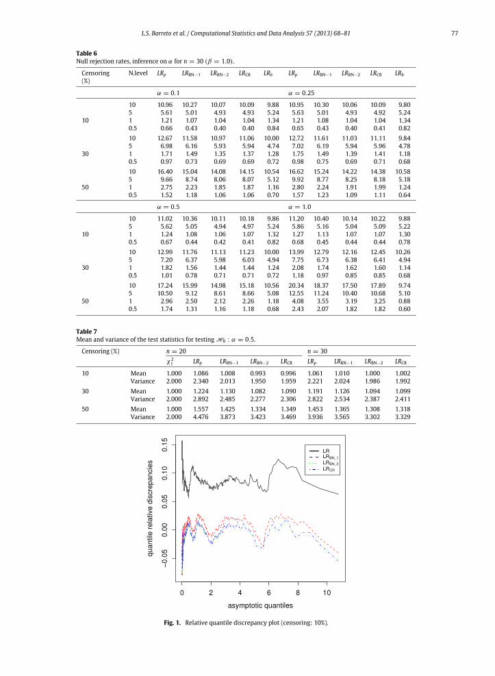
Table 7 contains the mean and variance of the LRp, LRBN−1, LRBN−2 and LRCR test statistics together with the first twoχ21 moments. The null hypothesis under test is H : α = 0.5. Data generation was carried out under the null hypothesis,

β = 1.00 and n = 20, 30. Notice that the LRBN−2 test statistic displays the best agreement between exact and asymptoticmoments; LRCR is the runner-up.

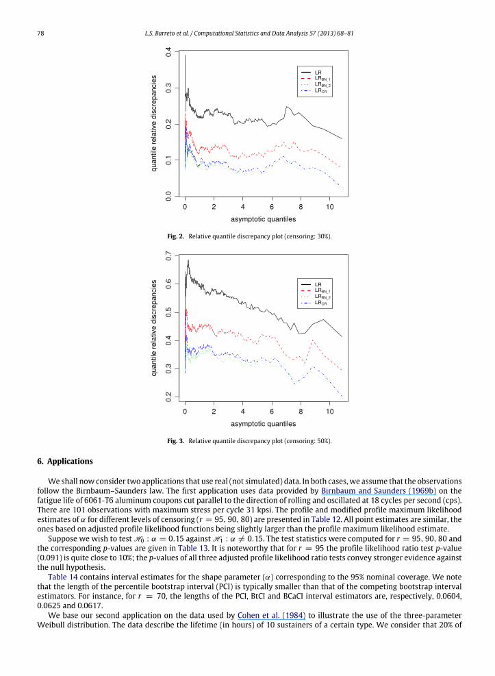
Figs. 1–3 are relative quantile discrepancy plots. We plot the relative quantile discrepancies (absolute differencesbetween exact and asymptotic quantiles divided by the latter) against asymptotic quantiles; n = 20 and differentlevels of censoring (10%, 30% and 50%, respectively). The closer to zero the relative quantile discrepancies, the better theapproximation of the exact null distribution by the asymptotic χ2

1 distribution. When only 10% of the observations arecensored (Fig. 1), LRBN−1, LRBN−2 and LRCR display very small relative quantile distortions, unlike LRp. The relative quantilediscrepancies becomemore pronounced as the proportion of censored observations increases (Figs. 2 and 3). Overall, LRBN−2is the winner. It typically displays the smallest relative quantile discrepancies.

Nonnull rejection rates (i.e., powers) are reported in Table 8. Since some of the tests are size-distorted, the tests werecarried out using exact (estimated from the size simulations) and not asymptotic critical values. We thus compare powers

74 L.S. Barreto et al. / Computational Statistics and Data Analysis 57 (2013) 68–81

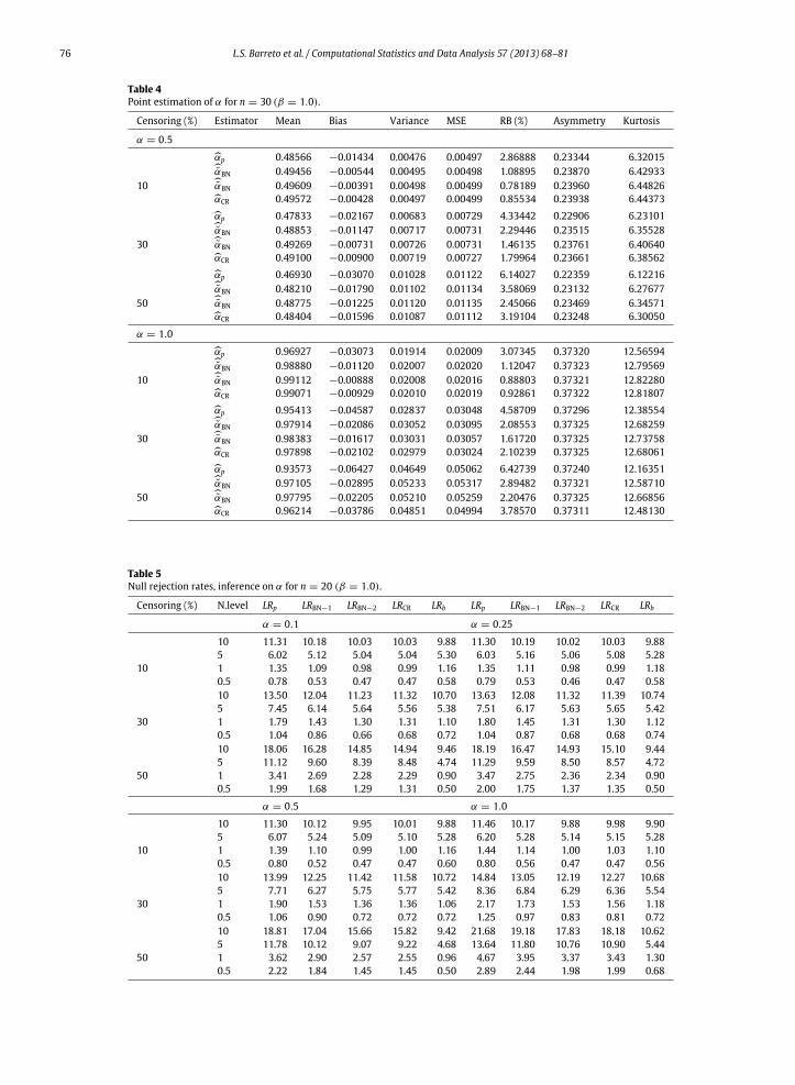
Table 1Point estimation of α for n = 20 (β = 1.0).

Censoring (%) Estimator Mean Bias Variance MSE RB (%) Asymmetry Kurtosis

α = 0.1 αp 0.09583 −0.00417 0.00028 0.00030 4.16936 0.01354 3.14088αBN 0.09837 −0.00163 0.00030 0.00030 1.62944 0.01425 3.1484310 αBN 0.09883 −0.00117 0.00030 0.00030 1.16713 0.01438 3.14983αCR 0.09876 −0.00124 0.00030 0.00030 1.23807 0.01436 3.14961αp 0.09393 −0.00607 0.00039 0.00043 6.06684 0.01301 3.13537αBN 0.09663 −0.00337 0.00042 0.00043 3.37380 0.01376 3.1432330 αBN 0.09808 −0.00192 0.00043 0.00043 1.92229 0.01417 3.14755αCR 0.09782 −0.00218 0.00043 0.00043 2.18221 0.01409 3.14677αp 0.09104 −0.00896 0.00059 0.00067 8.95794 0.01224 3.12718αBN 0.09406 −0.00594 0.00063 0.00066 5.94157 0.01305 3.1357350 αBN 0.09606 −0.00394 0.00065 0.00067 3.94478 0.01360 3.14154αCR 0.09581 −0.00419 0.00065 0.00066 4.18934 0.01353 3.14083

α = 0.25 αp 0.23950 −0.01050 0.00175 0.00186 4.20180 0.07725 3.86773αBN 0.24593 −0.00407 0.00185 0.00186 1.62681 0.08099 3.9140710 αBN 0.24710 −0.00290 0.00186 0.00187 1.16018 0.08167 3.92258αCR 0.24687 −0.00313 0.00186 0.00187 1.25388 0.08154 3.92087αp 0.23476 −0.01524 0.00247 0.00270 6.09796 0.07453 3.83433αBN 0.24175 −0.00825 0.00263 0.00270 3.29934 0.07855 3.8838430 αBN 0.24529 −0.00471 0.00270 0.00273 1.88264 0.08062 3.90941αCR 0.24435 −0.00565 0.00267 0.00271 2.25992 0.08007 3.90257αp 0.22754 −0.02246 0.00370 0.00420 8.98538 0.07045 3.78464αBN 0.23568 −0.01432 0.00400 0.00421 5.72837 0.07506 3.8407950 αBN 0.24056 −0.00944 0.00416 0.00425 3.77666 0.07786 3.87530αCR 0.23906 −0.01094 0.00406 0.00418 4.37613 0.07700 3.86463

of tests that are adjusted to have the correct size. (The bootstrap test is omitted from the analysis since it is not possible tosize-correct it.) The results were obtained using n = 20, β = 1.0 and values of α that range from 0.12 to 0.28. The nominallevels are 10% and 5% and all three levels of censoring are considered. The null hypothesis under test is H0 : α = 0.10. Thefigures in Table 8 show that LRp is less powerful than the adjusted profile likelihood ratio tests. The test that displays thesmallest overall type II error frequency is LRBN−2, closely followed by LRCR and LRBN−1. We also note that the tests becomeless powerful as the degree of censoring increases. For instance, when α = 0.16 and at the 10% nominal level, the powersof LRp, LRBN−1, LRBN−2 and LRCR are, respectively, 71.78%, 76.51%, 77.14% and 77.08%. When half of the observations arecensored, these rejection rates become 36.45%, 41.94%, 45.56% and 45.13%.

Tables 9 and 10 contain results on interval estimation. We report the empirical coverages (%) of the ACI, PCI, BtCIand BCaCI confidence intervals for α. The nominal coverage is 95%, all three levels of censoring are considered, α =

0.10, 0.25, 0.50, 1.00, β = 1.00 and n = 20 (Table 9) and n = 30 (Table 10). Overall, the best performing interval estimatoris BtCI (bootstrap-t). The BCa interval estimator is a close runner-up. The worst performer was PCI (percentile bootstrap).For instance, when α = 0.5, n = 30 (Table 10) and 30% of the observations are censored, the coverages of the ACI, PCI, BtCIand BCaCI confidence intervals are 89.34%, 86.72%, 94.60% and 94.20%, respectively.

5. Additional numerical results

We shall now compare the finite sample behavior of one of our modified profile likelihood estimators (αBN) to that of theestimator proposed by Ng et al. (2006), which is given by

α∗=α 1 −

1n

1 + 2.5

1 −

rn

−1

.

The numerical results are based on 10,000 Monte Carlo replications, n = 20 (twenty data points), α = 0.10, 0.25, 0.50, 1.0and the same three levels of censoring used in the previous evaluation (10%, 30% and 50%). Table 11 displays results relativeto the point estimation ofα. Notice thatαBN always has smaller variance andmean squared error thanα∗. For instance, whenα = 1.0 and half of the data points are subject to censoring, we have that var(αBN) = 0.08163 and var(α∗) = 0.08583;also, MSE(αBN) = 0.08251 and MSE(α∗) = 0.08621. Ou estimator is also less biased than the estimator proposed by Nget al. (2006), except when half of the observations are censored.

L.S. Barreto et al. / Computational Statistics and Data Analysis 57 (2013) 68–81 75

Table 2Point estimation of α for n = 20 (β = 1.0).

Censoring (%) Estimator Mean Bias Variance MSE RB (%) Asymmetry Kurtosis

α = 0.5 αp 0.47846 −0.02154 0.00699 0.00745 4.30780 0.22914 6.23263αBN 0.49181 −0.00819 0.00742 0.00749 1.63867 0.23708 6.3955010 αBN 0.49417 −0.00583 0.00749 0.00752 1.16621 0.23847 6.42457αCR 0.49357 −0.00643 0.00746 0.00751 1.28657 0.23812 6.41716αp 0.46898 −0.03102 0.00998 0.01094 6.20327 0.22340 6.11838αBN 0.48419 −0.01581 0.01075 0.01100 3.16147 0.23257 6.3023030 αBN 0.49065 −0.00935 0.01097 0.01106 1.86968 0.23640 6.38132αCR 0.48796 −0.01204 0.01079 0.01093 2.40733 0.23481 6.34837αp 0.45460 −0.04540 0.01525 0.01731 9.08084 0.21453 5.94736αBN 0.47354 −0.02646 0.01696 0.01766 5.29171 0.22617 6.1731750 αBN 0.48243 −0.01757 0.01744 0.01775 3.51384 0.23152 6.28084αCR 0.47649 −0.02351 0.01661 0.01716 4.70154 0.22795 6.20879

α = 1.0 αp 0.95378 −0.04622 0.02802 0.03016 4.62157 0.37295 12.38140αBN 0.98327 −0.01673 0.03016 0.03044 1.67350 0.37325 12.7309810 αBN 0.98743 −0.01257 0.03028 0.03044 1.25671 0.37324 12.77977αCR 0.98600 −0.01400 0.03018 0.03038 1.40032 0.37324 12.76298αp 0.93411 −0.06589 0.04132 0.04566 6.58923 0.37233 12.14385αBN 0.97161 −0.02839 0.04619 0.04700 2.83919 0.37322 12.5936830 αBN 0.98027 −0.01973 0.04610 0.04649 1.97287 0.37325 12.69584αCR 0.97126 −0.02874 0.04450 0.04532 2.87355 0.37322 12.58962αp 0.90474 −0.09526 0.06761 0.07668 9.52594 0.37075 11.78327αBN 0.95772 −0.04228 0.08126 0.08305 4.22823 0.37303 12.4284950 αBN 0.97028 −0.02972 0.08163 0.08251 2.97221 0.37321 12.57794αCR 0.94384 −0.05616 0.07214 0.07530 5.61615 0.37268 12.26174

Table 3Point estimation of α for n = 30 (β = 1.0).

Censoring (%) Estimator Mean Bias Variance MSE RB (%) Asymmetry Kurtosis

α = 0.1 αp 0.09722 −0.00278 0.00019 0.00020 2.77887 0.01392 3.14499αBN 0.09892 −0.00108 0.00020 0.00020 1.08188 0.01441 3.1500910 αBN 0.09924 −0.00076 0.00020 0.00020 0.76339 0.01450 3.15105αCR 0.09918 −0.00082 0.00020 0.00020 0.82397 0.01448 3.15087αp 0.09576 −0.00424 0.00027 0.00029 4.24016 0.01352 3.14068αBN 0.09757 −0.00243 0.00028 0.00029 2.43095 0.01402 3.1460330 αBN 0.09855 −0.00145 0.00029 0.00029 1.45391 0.01430 3.14896αCR 0.09835 −0.00165 0.00028 0.00029 1.64770 0.01424 3.14838αp 0.09396 −0.00604 0.00039 0.00043 6.03829 0.01302 3.13546αBN 0.09601 −0.00399 0.00041 0.00043 3.98996 0.01359 3.1414150 αBN 0.09732 −0.00268 0.00042 0.00043 2.67598 0.01395 3.14530αCR 0.09717 −0.00283 0.00042 0.00043 2.83452 0.01391 3.14483

α = 0.25 αp 0.24300 −0.00700 0.00119 0.00124 2.79995 0.07928 3.89282αBN 0.24730 −0.00270 0.00123 0.00124 1.08028 0.08179 3.9240510 αBN 0.24809 −0.00191 0.00124 0.00124 0.76321 0.08226 3.92986αCR 0.24791 −0.00209 0.00124 0.00124 0.83424 0.08215 3.92856αp 0.23935 −0.01065 0.00169 0.00180 4.26161 0.07716 3.86667αBN 0.24404 −0.00596 0.00176 0.00180 2.38238 0.07989 3.9003530 αBN 0.24641 −0.00359 0.00179 0.00181 1.43768 0.08127 3.91752αCR 0.24575 −0.00425 0.00178 0.00180 1.69949 0.08088 3.91274αp 0.23485 −0.01515 0.00248 0.00271 6.06114 0.07458 3.83497αBN 0.24037 −0.00963 0.00262 0.00271 3.85252 0.07775 3.8739550 αBN 0.24355 −0.00645 0.00268 0.00272 2.57872 0.07960 3.89681αCR 0.24260 −0.00740 0.00264 0.00270 2.96134 0.07904 3.88991

76 L.S. Barreto et al. / Computational Statistics and Data Analysis 57 (2013) 68–81

Table 4Point estimation of α for n = 30 (β = 1.0).

Censoring (%) Estimator Mean Bias Variance MSE RB (%) Asymmetry Kurtosis

α = 0.5 αp 0.48566 −0.01434 0.00476 0.00497 2.86888 0.23344 6.32015αBN 0.49456 −0.00544 0.00495 0.00498 1.08895 0.23870 6.4293310 αBN 0.49609 −0.00391 0.00498 0.00499 0.78189 0.23960 6.44826αCR 0.49572 −0.00428 0.00497 0.00499 0.85534 0.23938 6.44373αp 0.47833 −0.02167 0.00683 0.00729 4.33442 0.22906 6.23101αBN 0.48853 −0.01147 0.00717 0.00731 2.29446 0.23515 6.3552830 αBN 0.49269 −0.00731 0.00726 0.00731 1.46135 0.23761 6.40640αCR 0.49100 −0.00900 0.00719 0.00727 1.79964 0.23661 6.38562αp 0.46930 −0.03070 0.01028 0.01122 6.14027 0.22359 6.12216αBN 0.48210 −0.01790 0.01102 0.01134 3.58069 0.23132 6.2767750 αBN 0.48775 −0.01225 0.01120 0.01135 2.45066 0.23469 6.34571αCR 0.48404 −0.01596 0.01087 0.01112 3.19104 0.23248 6.30050

α = 1.0 αp 0.96927 −0.03073 0.01914 0.02009 3.07345 0.37320 12.56594αBN 0.98880 −0.01120 0.02007 0.02020 1.12047 0.37323 12.7956910 αBN 0.99112 −0.00888 0.02008 0.02016 0.88803 0.37321 12.82280αCR 0.99071 −0.00929 0.02010 0.02019 0.92861 0.37322 12.81807αp 0.95413 −0.04587 0.02837 0.03048 4.58709 0.37296 12.38554αBN 0.97914 −0.02086 0.03052 0.03095 2.08553 0.37325 12.6825930 αBN 0.98383 −0.01617 0.03031 0.03057 1.61720 0.37325 12.73758αCR 0.97898 −0.02102 0.02979 0.03024 2.10239 0.37325 12.68061αp 0.93573 −0.06427 0.04649 0.05062 6.42739 0.37240 12.16351αBN 0.97105 −0.02895 0.05233 0.05317 2.89482 0.37321 12.5871050 αBN 0.97795 −0.02205 0.05210 0.05259 2.20476 0.37325 12.66856αCR 0.96214 −0.03786 0.04851 0.04994 3.78570 0.37311 12.48130

Table 5Null rejection rates, inference on α for n = 20 (β = 1.0).

Censoring (%) N.level LRp LRBN−1 LRBN−2 LRCR LRb LRp LRBN−1 LRBN−2 LRCR LRb

α = 0.1 α = 0.25

10 11.31 10.18 10.03 10.03 9.88 11.30 10.19 10.02 10.03 9.885 6.02 5.12 5.04 5.04 5.30 6.03 5.16 5.06 5.08 5.28

10 1 1.35 1.09 0.98 0.99 1.16 1.35 1.11 0.98 0.99 1.180.5 0.78 0.53 0.47 0.47 0.58 0.79 0.53 0.46 0.47 0.5810 13.50 12.04 11.23 11.32 10.70 13.63 12.08 11.32 11.39 10.745 7.45 6.14 5.64 5.56 5.38 7.51 6.17 5.63 5.65 5.42

30 1 1.79 1.43 1.30 1.31 1.10 1.80 1.45 1.31 1.30 1.120.5 1.04 0.86 0.66 0.68 0.72 1.04 0.87 0.68 0.68 0.7410 18.06 16.28 14.85 14.94 9.46 18.19 16.47 14.93 15.10 9.445 11.12 9.60 8.39 8.48 4.74 11.29 9.59 8.50 8.57 4.72

50 1 3.41 2.69 2.28 2.29 0.90 3.47 2.75 2.36 2.34 0.900.5 1.99 1.68 1.29 1.31 0.50 2.00 1.75 1.37 1.35 0.50

α = 0.5 α = 1.0

10 11.30 10.12 9.95 10.01 9.88 11.46 10.17 9.88 9.98 9.905 6.07 5.24 5.09 5.10 5.28 6.20 5.28 5.14 5.15 5.28

10 1 1.39 1.10 0.99 1.00 1.16 1.44 1.14 1.00 1.03 1.100.5 0.80 0.52 0.47 0.47 0.60 0.80 0.56 0.47 0.47 0.5610 13.99 12.25 11.42 11.58 10.72 14.84 13.05 12.19 12.27 10.685 7.71 6.27 5.75 5.77 5.42 8.36 6.84 6.29 6.36 5.54

30 1 1.90 1.53 1.36 1.36 1.06 2.17 1.73 1.53 1.56 1.180.5 1.06 0.90 0.72 0.72 0.72 1.25 0.97 0.83 0.81 0.7210 18.81 17.04 15.66 15.82 9.42 21.68 19.18 17.83 18.18 10.625 11.78 10.12 9.07 9.22 4.68 13.64 11.80 10.76 10.90 5.44

50 1 3.62 2.90 2.57 2.55 0.96 4.67 3.95 3.37 3.43 1.300.5 2.22 1.84 1.45 1.45 0.50 2.89 2.44 1.98 1.99 0.68

L.S. Barreto et al. / Computational Statistics and Data Analysis 57 (2013) 68–81 77

Table 6Null rejection rates, inference on α for n = 30 (β = 1.0).

Censoring(%)

N.level LRp LRBN−1 LRBN−2 LRCR LRb LRp LRBN−1 LRBN−2 LRCR LRb

α = 0.1 α = 0.25

10 10.96 10.27 10.07 10.09 9.88 10.95 10.30 10.06 10.09 9.805 5.61 5.01 4.93 4.93 5.24 5.63 5.01 4.93 4.92 5.24

10 1 1.21 1.07 1.04 1.04 1.34 1.21 1.08 1.04 1.04 1.340.5 0.66 0.43 0.40 0.40 0.84 0.65 0.43 0.40 0.41 0.8210 12.67 11.58 10.97 11.06 10.00 12.72 11.61 11.03 11.11 9.845 6.98 6.16 5.93 5.94 4.74 7.02 6.19 5.94 5.96 4.78

30 1 1.71 1.49 1.35 1.37 1.28 1.75 1.49 1.39 1.41 1.180.5 0.97 0.73 0.69 0.69 0.72 0.98 0.75 0.69 0.71 0.6810 16.40 15.04 14.08 14.15 10.54 16.62 15.24 14.22 14.38 10.585 9.66 8.74 8.06 8.07 5.12 9.92 8.77 8.25 8.18 5.18

50 1 2.75 2.23 1.85 1.87 1.16 2.80 2.24 1.91 1.99 1.240.5 1.52 1.18 1.06 1.06 0.70 1.57 1.23 1.09 1.11 0.64

α = 0.5 α = 1.0

10 11.02 10.36 10.11 10.18 9.86 11.20 10.40 10.14 10.22 9.885 5.62 5.05 4.94 4.97 5.24 5.86 5.16 5.04 5.09 5.22

10 1 1.24 1.08 1.06 1.07 1.32 1.27 1.13 1.07 1.07 1.300.5 0.67 0.44 0.42 0.41 0.82 0.68 0.45 0.44 0.44 0.7810 12.99 11.76 11.13 11.23 10.00 13.99 12.79 12.16 12.45 10.265 7.20 6.37 5.98 6.03 4.94 7.75 6.73 6.38 6.41 4.94

30 1 1.82 1.56 1.44 1.44 1.24 2.08 1.74 1.62 1.60 1.140.5 1.01 0.78 0.71 0.71 0.72 1.18 0.97 0.85 0.85 0.6810 17.24 15.99 14.98 15.18 10.56 20.34 18.37 17.50 17.89 9.745 10.50 9.12 8.61 8.66 5.08 12.55 11.24 10.40 10.68 5.10

50 1 2.96 2.50 2.12 2.26 1.18 4.08 3.55 3.19 3.25 0.880.5 1.74 1.31 1.16 1.18 0.68 2.43 2.07 1.82 1.82 0.60

Table 7Mean and variance of the test statistics for testing H0 : α = 0.5.

Censoring (%) n = 20 n = 30χ21 LRp LRBN−1 LRBN−2 LRCR LRp LRBN−1 LRBN−2 LRCR

10 Mean 1.000 1.086 1.008 0.993 0.996 1.061 1.010 1.000 1.002Variance 2.000 2.340 2.013 1.950 1.959 2.221 2.024 1.986 1.992

30 Mean 1.000 1.224 1.130 1.082 1.090 1.191 1.126 1.094 1.099Variance 2.000 2.892 2.485 2.277 2.306 2.822 2.534 2.387 2.411

50 Mean 1.000 1.557 1.425 1.334 1.349 1.453 1.365 1.308 1.318Variance 2.000 4.476 3.873 3.423 3.469 3.936 3.565 3.302 3.329

Fig. 1. Relative quantile discrepancy plot (censoring: 10%).

78 L.S. Barreto et al. / Computational Statistics and Data Analysis 57 (2013) 68–81

Fig. 2. Relative quantile discrepancy plot (censoring: 30%).

Fig. 3. Relative quantile discrepancy plot (censoring: 50%).

6. Applications

We shall now consider two applications that use real (not simulated) data. In both cases, we assume that the observationsfollow the Birnbaum–Saunders law. The first application uses data provided by Birnbaum and Saunders (1969b) on thefatigue life of 6061-T6 aluminum coupons cut parallel to the direction of rolling and oscillated at 18 cycles per second (cps).There are 101 observations with maximum stress per cycle 31 kpsi. The profile and modified profile maximum likelihoodestimates of α for different levels of censoring (r = 95, 90, 80) are presented in Table 12. All point estimates are similar, theones based on adjusted profile likelihood functions being slightly larger than the profile maximum likelihood estimate.

Suppose we wish to test H0 : α = 0.15 against H1 : α = 0.15. The test statistics were computed for r = 95, 90, 80 andthe corresponding p-values are given in Table 13. It is noteworthy that for r = 95 the profile likelihood ratio test p-value(0.091) is quite close to 10%; the p-values of all three adjusted profile likelihood ratio tests convey stronger evidence againstthe null hypothesis.

Table 14 contains interval estimates for the shape parameter (α) corresponding to the 95% nominal coverage. We notethat the length of the percentile bootstrap interval (PCI) is typically smaller than that of the competing bootstrap intervalestimators. For instance, for r = 70, the lengths of the PCI, BtCI and BCaCI interval estimators are, respectively, 0.0604,0.0625 and 0.0617.

We base our second application on the data used by Cohen et al. (1984) to illustrate the use of the three-parameterWeibull distribution. The data describe the lifetime (in hours) of 10 sustainers of a certain type. We consider that 20% of

L.S. Barreto et al. / Computational Statistics and Data Analysis 57 (2013) 68–81 79

Table 8Nonnull rejection rates, inference on α.

Censoring (%) α N.level 10% N.level 5%LRp LRBN−1 LRBN−2 LRCR LRp LRBN−1 LRBN−2 LRCR

0.12 14.55 19.01 19.60 19.54 4.83 7.65 8.27 8.170.14 43.88 50.35 51.29 51.15 24.10 30.76 32.35 32.130.16 71.78 76.51 77.14 77.08 52.97 60.70 62.07 61.880.18 87.97 90.79 91.02 90.99 75.79 81.09 82.04 81.83

10 0.20 95.07 96.38 96.49 96.48 88.71 91.44 91.96 91.910.22 98.34 98.82 98.87 98.87 95.50 96.81 97.03 96.980.24 99.12 99.35 99.38 99.38 97.78 98.43 98.59 98.580.26 99.66 99.84 99.86 99.86 99.13 99.36 99.41 99.400.28 99.89 99.92 99.94 99.94 99.72 99.80 99.81 99.810.12 9.69 12.92 14.43 14.20 2.60 4.24 5.13 5.000.14 30.22 36.25 38.68 38.20 14.97 19.86 22.11 21.830.16 53.85 59.69 62.29 61.82 35.30 42.08 44.78 44.520.18 73.75 78.10 79.84 79.58 57.31 63.46 66.17 65.81

30 0.20 85.26 88.34 89.44 89.26 73.96 78.66 80.27 80.140.22 92.19 93.80 94.53 94.44 84.31 87.81 89.00 88.910.24 95.85 96.75 97.10 97.07 91.56 93.52 94.15 94.080.26 97.88 98.34 98.58 98.52 95.30 96.50 96.74 96.720.28 98.89 99.24 99.36 99.33 97.53 98.08 98.29 98.280.12 7.08 9.17 10.95 10.68 1.87 2.61 3.69 3.490.14 18.97 23.10 26.63 26.16 8.61 10.98 13.33 13.110.16 36.45 41.94 45.56 45.13 21.35 25.47 29.66 29.170.18 53.34 58.77 62.18 61.80 36.44 41.65 45.96 45.43

50 0.20 67.14 71.69 74.69 74.39 53.01 57.08 61.06 60.540.22 78.02 81.43 83.50 83.33 65.85 69.71 72.97 72.600.24 85.51 87.71 89.45 89.24 76.54 79.58 81.97 81.680.26 90.01 91.84 92.77 92.65 83.18 85.66 87.61 87.410.28 93.39 94.59 95.41 95.32 88.25 89.97 91.30 91.21

Table 9Confidence interval coverages (95%) for α (β = 1.0 and n = 20).

Censoring (%) ACI PCI BtCI BCaCI ACI PCI BtCI BCaCI

α = 0.1 α = 0.25

10 88.98 86.66 95.04 94.52 88.96 86.54 95.06 94.4830 86.66 83.14 95.14 93.32 86.64 83.04 95.16 93.3850 82.80 79.30 94.60 90.80 82.70 79.20 94.50 90.86

α = 0.5 α = 1.0

10 88.74 86.34 95.04 94.32 88.48 85.62 94.96 94.1830 86.42 82.92 95.00 93.20 85.86 82.42 94.66 92.9850 82.60 79.02 94.20 90.80 81.26 77.94 92.92 90.46

Table 10Confidence interval coverages (95%) for α (β = 1.0 and n = 30).

Censoring (%) ACI PCI BtCI BCaCI ACI PCI BtCI BCaCI

α = 0.1 α = 0.25

10 90.94 88.84 95.00 94.92 90.88 88.80 95.06 94.9030 89.40 87.02 94.66 94.36 89.40 87.02 94.68 94.3050 86.54 83.54 94.52 93.46 86.46 83.54 94.36 93.36

α = 0.5 α = 1.0

10 90.84 88.68 95.06 94.82 90.58 88.20 94.94 94.7830 89.34 86.72 94.60 94.20 88.94 86.26 94.52 94.0850 86.08 83.50 94.08 93.40 85.50 82.94 92.98 93.40

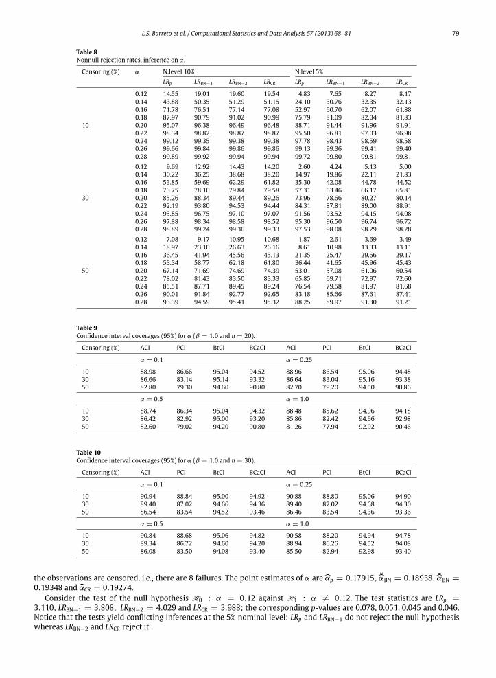
the observations are censored, i.e., there are 8 failures. The point estimates of α areαp = 0.17915,αBN = 0.18938,αBN =

0.19348 andαCR = 0.19274.Consider the test of the null hypothesis H0 : α = 0.12 against H1 : α = 0.12. The test statistics are LRp =

3.110, LRBN−1 = 3.808, LRBN−2 = 4.029 and LRCR = 3.988; the corresponding p-values are 0.078, 0.051, 0.045 and 0.046.Notice that the tests yield conflicting inferences at the 5% nominal level: LRp and LRBN−1 do not reject the null hypothesiswhereas LRBN−2 and LRCR reject it.

80 L.S. Barreto et al. / Computational Statistics and Data Analysis 57 (2013) 68–81

Table 11Point estimation of α for n = 20 (β = 1.0).

α Censoring(%)

RB (αp) Variance(αp)

MSE(αp)

RB(αBN)

Variance(αBN)

MSE(αBN)

RB (α∗) Variance(α∗)

MSE(α∗)

10 4.16936 0.00028 0.00030 1.16713 0.00030 0.00030 2.21935 0.00032 0.000320.1 30 6.06684 0.00039 0.00043 1.92229 0.00043 0.00043 2.94045 0.00047 0.00048

50 8.95794 0.00059 0.00067 3.94478 0.00065 0.00067 2.58261 0.00074 0.0007510 4.20180 0.00175 0.00186 1.16018 0.00186 0.00187 2.18475 0.00199 0.00202

0.25 30 6.09796 0.00247 0.00270 1.88264 0.00270 0.00273 2.90634 0.00297 0.0030250 8.98538 0.00370 0.00420 3.77666 0.00416 0.00425 2.55169 0.00469 0.0047310 4.30780 0.00699 0.00745 1.16621 0.00749 0.00752 2.07168 0.00795 0.00806

0.5 30 6.20327 0.00998 0.01094 1.86968 0.01097 0.01106 2.79093 0.01198 0.0121750 9.08084 0.01525 0.01731 3.51384 0.01744 0.01775 2.44412 0.01936 0.0195110 4.62157 0.02802 0.03016 1.25671 0.03028 0.03044 1.73699 0.03188 0.03218

1.0 30 6.58923 0.04132 0.04566 1.97287 0.04610 0.04649 2.36797 0.04962 0.0501850 9.52594 0.06761 0.07668 2.97221 0.08163 0.08251 1.94261 0.08583 0.08621

Table 12Profile and adjusted profile maximum likelihood estimates of α—first application.

r αp αBN−1 αBN−2 αCR

95 0.16906 0.16992 0.17002 0.1699990 0.17061 0.17149 0.17168 0.1716280 0.17505 0.17599 0.17637 0.17625

Table 13p-values—first application.

r LRp LRBN−1 LRBN−2 LRCR

95 0.091 0.079 0.078 0.07890 0.079 0.068 0.066 0.06780 0.048 0.041 0.039 0.040

Table 14Confidence intervals for α—first application.

r Interval Lower limit Upper limit Width

90 ACI 0.1450 0.1962 0.0512PCI 0.1457 0.1959 0.0502BtCI 0.1487 0.1997 0.0510BCaCI 0.1495 0.2013 0.0518

70 ACI 0.1429 0.2041 0.0612PCI 0.1423 0.2027 0.0604BtCI 0.1486 0.2112 0.0625BCaCI 0.1487 0.2104 0.0617

50 ACI 0.1448 0.2249 0.0801PCI 0.1428 0.2235 0.0807BtCI 0.1533 0.2384 0.0851BCaCI 0.1525 0.2392 0.0867

Table 15Confidence intervals for α—second application.

Interval Lower limit Upper limit Width

ACI 0.0868 0.2715 0.1847PCI 0.0756 0.2587 0.1831BtCI 0.1238 0.4263 0.3025BCaCI 0.1249 0.3586 0.2337

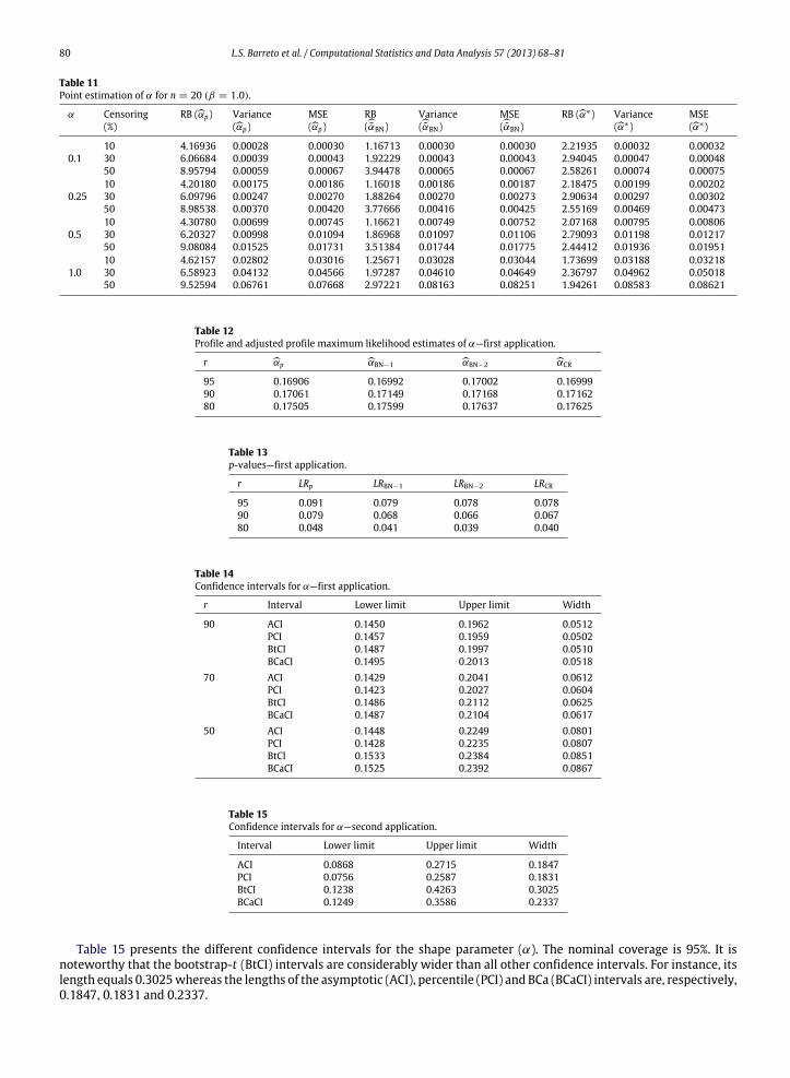
Table 15 presents the different confidence intervals for the shape parameter (α). The nominal coverage is 95%. It isnoteworthy that the bootstrap-t (BtCI) intervals are considerably wider than all other confidence intervals. For instance, itslength equals 0.3025whereas the lengths of the asymptotic (ACI), percentile (PCI) and BCa (BCaCI) intervals are, respectively,0.1847, 0.1831 and 0.2337.

L.S. Barreto et al. / Computational Statistics and Data Analysis 57 (2013) 68–81 81

7. Concluding remarks

We have developed adjusted profile likelihood inference for the Birnbaum–Saunders shape parameter under type IIcensoring. We have also considered bootstrap-based inference: hypothesis testing and interval estimation. In particular,interval estimation is carried out using three different bootstrapping strategies, namely: the percentile, bootstrap-t andbias corrected accelerated confidence intervals. We have also presented and discussed the results of extensive MonteCarlo simulations on point estimation, interval estimation and hypothesis testing. The best performing point estimatorwas that obtained from the maximization of Barndorff-Nielsen’s (1983) adjusted profile log-likelihood function. It typicallydisplayed the smallest relative bias. Our results also revealed that when only a few observations are censored (e.g., 10% ofall observations) both the adjusted profile likelihood ratio tests and the bootstrap test deliver reliable inference. However,when a sizable proportion of the observations are subject to censoring (30%–50%, for example), the bootstrap test clearlyoutperforms the tests obtained from adjusted profile likelihood functions. Finally, the numerical results favor intervalestimation through the bootstrap-t confidence interval, the BCa confidence interval being the runner-up.

Acknowledgments

We gratefully acknowledge financial support from CAPES, CNPq and FACEPE. We also thank two anonymous referees forcomments and suggestions.

References

Barndorff-Nielsen, O.E., 1983. On a formula to the distribution of the maximum likelihood estimator. Biometrika 70, 343–365.Birnbaum, Z.W., Saunders, S.C., 1969a. A new family of life distribution. Journal of Applied Probability 6, 319–327.Birnbaum, Z.W., Saunders, S.C., 1969b. Estimation for a family of life distributions with applications to fatigue. Journal of Applied Probability 6, 328–347.Cohen, A.C., Whitten, B.J., Ding, Y., 1984. Modified moment estimation for the three-parameter Weibull distribution. Journal of Quality Technology 16,

159–167.Cox, D.R., Reid, N., 1987. Parameter orthogonality and approximate conditional inference. Journal of the Royal Statistical Society. Series B 49, 1–39.Cysneiros, A.H.M.A., Cribari-Neto, F., Araújo Júnior, C.A.G., 2008. On Birnbaum–Saunders inference. Computational Statistics and Data Analysis 80, 1–21.Davison, A.C., Hinkley, D.V., 1997. Bootstrap Methods and their Application. Cambridge University Press, New York.Desmond, A.F., 1985. Stochastic models of failure in random environments. Canadian Journal of Statistics 13, 171–183.Desmond, A.F., 1986. On the relationship between two fatigue-life models. IEEE Transactions on Reliability 35, 167–169.Díaz-Garcia, J.A., Leiva-Sánchez, V., 2005. A new family of life distributions based on the elliptically contoured distributions. Journal of Statistical Planning

and Inference 128, 445–457.Doornik, J.A., 2009. An Object-Oriented Matrix Programming Language Ox6. London: Timberlake Consultants and Oxford. http://www.doornik.com.Efron, B., 1979. Bootstrap methods: another look at the jackknife. Annals of Statistics 7, 1–26.Fraser, D.A.S., Reid, N., 1995. Ancillaries and third-order significance. Utilitas Mathematica 47, 33–53.Fraser, D.A.S., Reid, N., Wu, J., 1999. A simple formula for tail probabilities for frequentist and Bayesian inference. Biometrika 86, 655–661.Galea, M., Leiva-Sánchez, V., Paula, G.A., 2004. Influence diagnostics in log-Birnbaum–Saunders regression models. Journal of Applied Statistics 31,

1049–1064.Lemonte, A.J., Cribari-Neto, F., Vasconcellos, K.L.P., 2007. Improved statistical inference for the two-parameter Birnbaum–Saunders distribution.

Computational Statistics and Data Analysis 51, 4656–4681.Ng, H.K.T., Kundu, D., Balakrishnan, N., 2003. Modified moment estimation for the two parameters Birnbaum–Saunders distribution. Computational

Statistics and Data Analysis 43, 283–298.Ng, H.K.T., Kundu, D., Balakrishnan, N., 2006. Point and interval estimation for the two-parameter Birnbaum–Saunders distribution based on type-II

censored samples. Computational Statistics and Data Analysis 50, 3222–3242.Nocedal, J., Wright, S.J., 1999. Numerical Optimization. Springer, New York.Pace, L., Salvan, A., 1997. Principles of Statistical Inference from a Neo-Fisherian Perspective. World Scientific, Singapore.Severini, T.A., 1998. An approximation to the modified profile likelihood function. Biometrika 85, 403–411.Severini, T.A., 1999. An empirical adjustment to the likelihood ratio statistic. Biometrika 86, 235–247.Severini, T.A., 2000. Likelihood Methods in Statistics. Oxford University Press, Oxford.Wang, Z., Desmond, A.F., Lu, X., 2006. Modified censored moment estimation for the two-parameter Birnbaum–Saunders distribution. Computational

Statistics and Data Analysis 50, 1033–1051.Wu, J., Wong, A.C.M., 1994. Improved interval estimation for the two-parameter Birnbaum–Saunders distribution. Computational Statistics and Data

Analysis 47, 809–821.