Importance of the subgrid-scale turbulent moist process: Cloud distribution in global cloud-resolving simulations

Atmospheric Research 96 (2010) 208–217

Contents lists available at ScienceDirect

Atmospheric Research

j ourna l homepage: www.e lsev ie r.com/ locate /atmos

Importance of the subgrid-scale turbulent moist process: Cloud distributionin global cloud-resolving simulations

Akira T. Noda a,⁎, Kazuyoshi Oouchi a, Masaki Satoh a,b, Hirofumi Tomita a,Shin-ichi Iga a, Yoko Tsushima a

a Research Institute for Global Change, Japan Agency for Marine-Earth Science and Technology, 3173-25 Showamachi, Kanazawa-ku, Yokohama City,Kanagawa 236-0001, Japanb Center for Climate System Research, The University of Tokyo, 5-1-5 Kashiwanoha, Chiba 277-8568, Japan

a r t i c l e i n f o

⁎ Corresponding author. Tel.: +81 45 778 5586; faxE-mail address: [email protected] (A.T. Noda)

0169-8095/$ – see front matter © 2009 Elsevier B.V.doi:10.1016/j.atmosres.2009.05.007

a b s t r a c t

Article history:Received 2 December 2008Revised in revised form 18 March 2009Accepted 12 May 2009

This study investigated the turbulent transport process within the nonhydrostatic icosahedralatmospheric model (NICAM), a global cloud-resolving model (GCRM), with particular focus onthe spatial reproducibility of cloud characteristics in NICAM simulations. A turbulent closuremodel was applied, based on level 2 of the model developed by Nakanishi and Niino([Nakanishi, M., and Niino, H., 2006: An improvedMellor–Yamada level-3 model: its numericalstability and application to a regional prediction of advection fog. Boundary-Layer Meteorol.,119, 397–407.]; a revised version of the original Mellor–Yamada model), together with asubgrid-scale condensation process.NICAM simulations were conducted for boreal summer of 2004 using mesh sizes of about14 km and 7 km. Simulated cloud amounts and radiative budget were compared with observeddata. The results confirmed an improvement in the spatial distribution of low clouds thatdevelop in offshore regions of subtropical continents compared to past NICAM experiments([Iga, S., Tomita, H., Tsushima, Y., and Satoh, M., 2007: Climatology of a nonhydrostatic globalmodel with explicit cloud process. Geophys. Res. Lett., 34, L22814, doi:10.1029/2007/GL031048.]). A sensitivity study of subgrid-scale clouds in the turbulent closure schemerevealed that the turbulent transport process modulated by the subgrid-scale cloud stronglycontrols not only the low-cloud amount but also mid- and high-cloud amounts. This indicatesthat parameterization of unresolvable subgrid-scale clouds remains an important componentof cloud behavior in GCRMs.

© 2009 Elsevier B.V. All rights reserved.

Keywords:Global cloud-resolving modelTurbulenceClimatology of cloud amountHigh-resolution simulation

1. Introduction

Global cloud-resolving models (GCRMs) are expected toresult in considerable dimensional changes to global atmo-spheric simulations, particularly with regard to tropical clouddisturbances. The nonhydrostatic icosahedral atmosphericmodel (NICAM; Tomita and Satoh, 2004; Satoh et al., 2008)was designed to incorporate this kind of data, and severalsuccessful experiments have already been conducted on

: +81 45 778 5706..

All rights reserved.

tropical cloud disturbances such as the Madden–JulianOscillations and tropical cyclones (Tomita et al., 2005;Miura et al., 2007a,b; Nasuno et al., 2007, 2009; Fudeyasuet al., 2008; Oouchi et al., 2009). Comparisons of GCRM-simulated cloud data with observed data have revealed goodagreement between observed and simulated values (Iga et al.,2007; Inoue et al., 2008).

GCRMs have remarkable advantages against conventionalgeneral circulation models (GCMs): they can reduce uncer-tainties raised by cumulus parameterization. GCRMs gener-ally use a mesh size smaller than 5 km; thus the 3.5-kmmeshNICAM experiments conducted by Tomita et al. (2005)and Miura et al. (2007a,b) can be categorized as GCRM

209A.T. Noda et al. / Atmospheric Research 96 (2010) 208–217

experiments in a narrow sense. In this paper, GCRMs areloosely defined as atmospheric global models without theuse of cumulus parameterization; by this definition, theglobal 14-km mesh and 7-km mesh experiments conductedby Miura et al. (2007a) and Iga et al. (2007) can also beclassified as GCRM experiments. This is not to say that GCRMsdo not require subgrid schemes; current GCRMs with a meshsize larger than a few kilometers cannot resolve small-scaleatmospheric phenomena including boundary-layer (BL)clouds and associated changes in turbulent transport. Hor-izontal mesh size must not exceed 100 m to permit an explicitresolution of BL clouds; this requires a global large-eddymodel and considerably more computer resources. Therefore,parameterization of the turbulent transport process is one ofthe most pressing issues for improving the physical perfor-mance of GCRMs. Miura et al. (2007a) reported that in theirGCRM simulations, the turbulent transport process affectedthe development of typhoon evolution. Low-cloud behav-ior also greatly affects climate sensitivity in climate models(Bony and Dufresne, 2005; Medeiros et al., 2008).

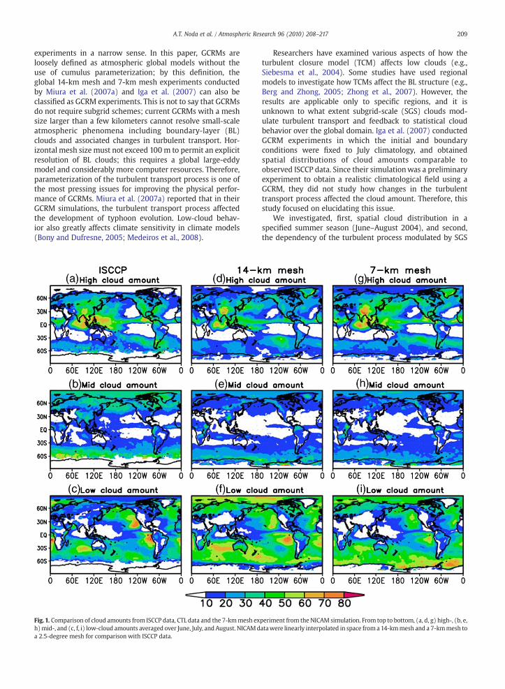
Fig. 1. Comparison of cloud amounts from ISCCP data, CTL data and the 7-kmmesh exh)mid-, and (c, f, i) low-cloud amounts averaged over June, July, and August. NICAMda 2.5-degree mesh for comparison with ISCCP data.

Researchers have examined various aspects of how theturbulent closure model (TCM) affects low clouds (e.g.,Siebesma et al., 2004). Some studies have used regionalmodels to investigate how TCMs affect the BL structure (e.g.,Berg and Zhong, 2005; Zhong et al., 2007). However, theresults are applicable only to specific regions, and it isunknown to what extent subgrid-scale (SGS) clouds mod-ulate turbulent transport and feedback to statistical cloudbehavior over the global domain. Iga et al. (2007) conductedGCRM experiments in which the initial and boundaryconditions were fixed to July climatology, and obtainedspatial distributions of cloud amounts comparable toobserved ISCCP data. Since their simulationwas a preliminaryexperiment to obtain a realistic climatological field using aGCRM, they did not study how changes in the turbulenttransport process affected the cloud amount. Therefore, thisstudy focused on elucidating this issue.

We investigated, first, spatial cloud distribution in aspecified summer season (June–August 2004), and second,the dependency of the turbulent process modulated by SGS

periment from the NICAM simulation. From top to bottom, (a, d, g) high-, (b, e,atawere linearly interpolated in space froma 14-kmmesh and a 7-kmmesh to

210 A.T. Noda et al. / Atmospheric Research 96 (2010) 208–217

clouds on statistical cloud behavior. To do this, we choseparticular months in boreal summer of 2004 for the NICAMsimulation. We also developed a possible TCM implementa-tion for GCRMs. Our detailed analyses of temporal variations,such as seasonal-scale changes and relations with dynamicalenvironmental fields, will be presented in separate papers.

2. Model setup

2.1. Experimental design

We conducted experiments for boreal summer of 2004using horizontal mesh sizes of approximately 14 km and7 km. The 14-km mesh experiment was conducted for5 months (June–October), and the 7-km mesh experimentwas conducted for 3 months (June–August). Our overall goalwas to observe inter-seasonal changes in monsoon circula-tions, but this paper focuses simply on statistical cloudbehavior. To this end, we used 3-monthmean data from June–August in our analysis of the 14-km mesh experiment; thisexperiment is referred to as CTL. To test the sensitivity of thelow cloud, we selected the first 10 days and conductedexperiments for the same period while changing the SGSparameters, as shown in Section 4.

We briefly compare the 7-km mesh experiment with the14-km mesh experiment (Figs. 1 and 2) because a detailedanalysis of resolution dependency is not themain focus of thispaper. A 14-km mesh is insufficient to resolve individualclouds, but our previous research (Miura et al., 2007a,b; Iga etal., 2007) has suggested that the 14-km mesh model canreproduce gross behaviors of cloud ensembles of deepconvections, and it is an acceptable tool for investigating

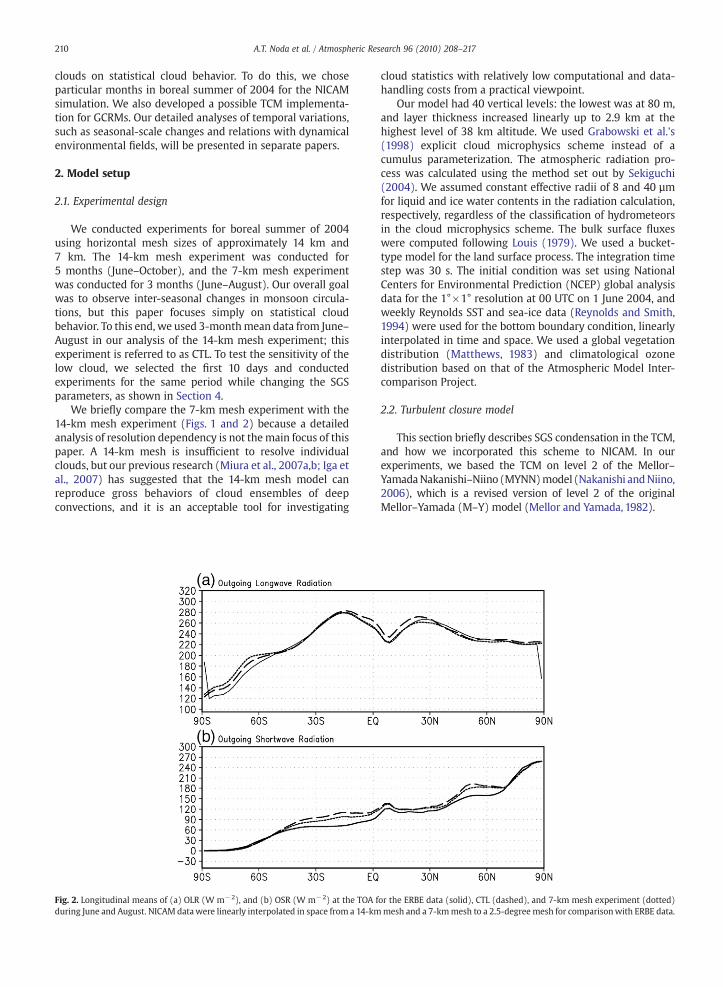
Fig. 2. Longitudinal means of (a) OLR (W m−2), and (b) OSR (W m−2) at the TOA fduring June and August. NICAM datawere linearly interpolated in space from a 14-km

cloud statistics with relatively low computational and data-handling costs from a practical viewpoint.

Our model had 40 vertical levels: the lowest was at 80 m,and layer thickness increased linearly up to 2.9 km at thehighest level of 38 km altitude. We used Grabowski et al.'s(1998) explicit cloud microphysics scheme instead of acumulus parameterization. The atmospheric radiation pro-cess was calculated using the method set out by Sekiguchi(2004). We assumed constant effective radii of 8 and 40 µmfor liquid and ice water contents in the radiation calculation,respectively, regardless of the classification of hydrometeorsin the cloud microphysics scheme. The bulk surface fluxeswere computed following Louis (1979). We used a bucket-type model for the land surface process. The integration timestep was 30 s. The initial condition was set using NationalCenters for Environmental Prediction (NCEP) global analysisdata for the 1°×1° resolution at 00 UTC on 1 June 2004, andweekly Reynolds SST and sea-ice data (Reynolds and Smith,1994) were used for the bottom boundary condition, linearlyinterpolated in time and space. We used a global vegetationdistribution (Matthews, 1983) and climatological ozonedistribution based on that of the Atmospheric Model Inter-comparison Project.

2.2. Turbulent closure model

This section briefly describes SGS condensation in the TCM,and how we incorporated this scheme to NICAM. In ourexperiments, we based the TCM on level 2 of the Mellor–YamadaNakanishi–Niino (MYNN)model (Nakanishi andNiino,2006), which is a revised version of level 2 of the originalMellor–Yamada (M–Y) model (Mellor and Yamada, 1982).

or the ERBE data (solid), CTL (dashed), and 7-km mesh experiment (dotted)mesh and a 7-kmmesh to a 2.5-degree mesh for comparisonwith ERBE data

211A.T. Noda et al. / Atmospheric Research 96 (2010) 208–217

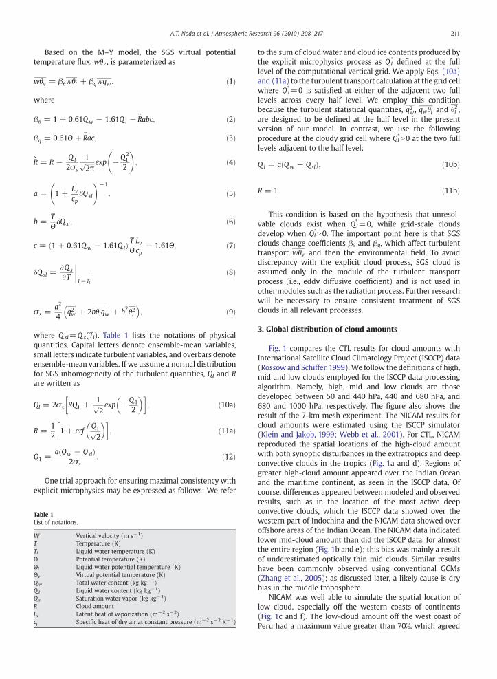
Based on the M–Y model, the SGS virtual potentialtemperature flux, wθv , is parameterized as

wθv = βθwθl + βqwqw ; ð1Þ

where

βθ = 1 + 0:61Qw − 1:61Q l − R̃abc; ð2Þ

βq = 0:61Θ + R̃ac; ð3Þ

R̃ = R − Q l

2σ s

1ffiffiffiffiffiffi2π

p exp −Q21

2

!; ð4Þ

a = 1 +Lvcp

δQ sl

!−1

; ð5Þ

b =TΘδQ sl; ð6Þ

c = 1 + 0:61Qw − 1:61Q lð Þ TΘLvcp

− 1:61Θ; ð7Þ

δQ sl =AQ s

AT jT=Tl

; ð8Þ

σ s =a2

4q2w + 2bθlqw + b2θ2l� �

; ð9Þ

where Q sl=Q s(Tl). Table 1 lists the notations of physicalquantities. Capital letters denote ensemble-mean variables,small letters indicate turbulent variables, and overbars denoteensemble-mean variables. If we assume a normal distributionfor SGS inhomogeneity of the turbulent quantities, Ql and Rare written as

Ql = 2σ s RQ1 +1ffiffiffi2

p exp −Q1

2

� �� �; ð10aÞ

R =12

1 + erfQ1ffiffiffi2

p� �� �

; ð11aÞ

Q1 =a Qw − Qslð Þ

2σ s: ð12Þ

One trial approach for ensuring maximal consistency withexplicit microphysics may be expressed as follows: We refer

Table 1List of notations.

W Vertical velocity (m s−1)T Temperature (K)Tl Liquid water temperature (K)Θ Potential temperature (K)Θl Liquid water potential temperature (K)Θv Virtual potential temperature (K)Qw Total water content (kg kg−1)Q l Liquid water content (kg kg−1)Q s Saturation water vapor (kg kg−1)R Cloud amountLv Latent heat of vaporization (m−2 s−2)cp Specific heat of dry air at constant pressure (m−2 s−2 K−1)

to the sum of cloud water and cloud ice contents produced bythe explicit microphysics process as Ql

* defined at the fulllevel of the computational vertical grid. We apply Eqs. (10a)and (11a) to the turbulent transport calculation at the grid cellwhere Ql

*=0 is satisfied at either of the adjacent two fulllevels across every half level. We employ this conditionbecause the turbulent statistical quantities, q2w , qwθl and θ2l ,are designed to be defined at the half level in the presentversion of our model. In contrast, we use the followingprocedure at the cloudy grid cell where Ql

*N0 at the two fulllevels adjacent to the half level:

Q l = a Qw − Q slð Þ; ð10bÞ

R = 1: ð11bÞ

This condition is based on the hypothesis that unresol-vable clouds exist when Ql

*=0, while grid-scale cloudsdevelop when Ql

*N0. The important point here is that SGSclouds change coefficients βθ and βq, which affect turbulenttransport wθv and then the environmental field. To avoiddiscrepancy with the explicit cloud process, SGS cloud isassumed only in the module of the turbulent transportprocess (i.e., eddy diffusive coefficient) and is not used inother modules such as the radiation process. Further researchwill be necessary to ensure consistent treatment of SGSclouds in all relevant processes.

3. Global distribution of cloud amounts

Fig. 1 compares the CTL results for cloud amounts withInternational Satellite Cloud Climatology Project (ISCCP) data(Rossow and Schiffer,1999).We follow the definitions of high,mid and low clouds employed for the ISCCP data processingalgorithm. Namely, high, mid and low clouds are thosedeveloped between 50 and 440 hPa, 440 and 680 hPa, and680 and 1000 hPa, respectively. The figure also shows theresult of the 7-km mesh experiment. The NICAM results forcloud amounts were estimated using the ISCCP simulator(Klein and Jakob, 1999; Webb et al., 2001). For CTL, NICAMreproduced the spatial locations of the high-cloud amountwith both synoptic disturbances in the extratropics and deepconvective clouds in the tropics (Fig. 1a and d). Regions ofgreater high-cloud amount appeared over the Indian Oceanand the maritime continent, as seen in the ISCCP data. Ofcourse, differences appeared between modeled and observedresults, such as in the location of the most active deepconvective clouds, which the ISCCP data showed over thewestern part of Indochina and the NICAM data showed overoffshore areas of the Indian Ocean. The NICAM data indicatedlower mid-cloud amount than did the ISCCP data, for almostthe entire region (Fig. 1b and e); this bias was mainly a resultof underestimated optically thin mid clouds. Similar resultshave been commonly observed using conventional GCMs(Zhang et al., 2005); as discussed later, a likely cause is drybias in the middle troposphere.

NICAM was well able to simulate the spatial location oflow cloud, especially off the western coasts of continents(Fig. 1c and f). The low-cloud amount off the west coast ofPeru had a maximum value greater than 70%, which agreed

212 A.T. Noda et al. / Atmospheric Research 96 (2010) 208–217

well with the ISCCP data. However, the NICAM data indicatedthat the low-cloud amounts off the coasts of California andNamibia would generally be less than 60%, a slight under-estimation. In mid- and high-latitudes, low clouds weresystematically overproduced; this was probably related to themoist bias that mainly appeared in the lower atmosphere,compared to NCEP analysis data as will be shown in Fig. 5a.The mid- and high-cloud amounts in the 7-km meshexperiment are qualitatively similar to those in CTL (Fig. 1g,h and i) while the low-cloud amount tended to decreaseoverall. The change in the low-cloud amount consequentlydecreased the positive bias observed in the tropical region(e.g., at around 130°W, 10°S) and in the subtropical regionover Oceania. However, the systematic development of lowcloud over the west coastal regions of the continents becamesomewhat weaker.

Fig. 2 compares the longitudinal means for outgoinglongwave radiation (OLR) and outgoing shortwave radiation(OSR) at the top of the atmosphere (TOA) in the CTL and 7-kmmesh experiments with Earth Radiation Budget Experiment(ERBE) data (Harrison et al., 1990). The NICAM OLR distribu-tion was almost identical to observed results, indicating that

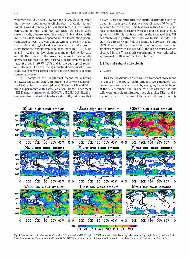
Fig. 3. Comparison of cloud amounts: CTL (left), DRY (center), andWET (right) NICAlow-cloud amounts (5-day mean; 6–10 June 2004). NICAM data were linearly inter

NICAM is able to reproduce the spatial distribution of highclouds in the tropics. A positive bias of about 10 W m−2

appeared for the tropics; this bias was reduced in the 7-kmmesh experiment, consistent with the findings published byIga et al. (2007). In contrast, OSR results indicated that CTLhas much larger positive bias from low-to mid-latitudes; thebias is up to 35 W m−2 in the latitudes between 15°S and50°N. This result was mainly due to excessive low-cloudamounts, as shown in Fig.1c and f. Although a similar bias wasobserved in the 7-km mesh experiment, it was reduced toapproximately 10 W m−2 in the subtropics.

4. Effects of subgrid-scale clouds

4.1. Setup

This section discusses the turbulent transport process andits effect on the spatial cloud amount. We conducted twodistinct sensitivity experiments by changing the formulationof the SGS turbulent flux: in one case, we assumed the gridcells were entirely unsaturated (i.e., clear sky; DRY), and inthe other case, we assumed the grid cells were entirely

M simulation data. From top to bottom, (a, d, g) high, (b, e, h) mid, and (c, f, i)polated in space from a 14-km mesh to a 2.5-degree mesh as in Fig. 1.

213A.T. Noda et al. / Atmospheric Research 96 (2010) 208–217

saturated (i.e., cloudy sky; WET). These assumptions wereachieved by modifying the computation of turbulent flux,respectively, as follows:

R̃Y0andRY0;

Ql = a Qw − Qslð Þ andRY1;

forDRY

forWET:

The modification for WET is similar to modifications usedin a sensitivity study conducted by Miura et al. (2007a), inwhich the threshold value of cloud water for the moist

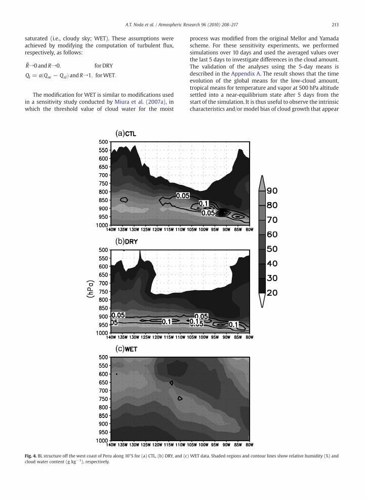
Fig. 4. BL structure off the west coast of Peru along 10°S for (a) CTL, (b) DRY, and (c)cloud water content (g kg−1), respectively.

process was modified from the original Mellor and Yamadascheme. For these sensitivity experiments, we performedsimulations over 10 days and used the averaged values overthe last 5 days to investigate differences in the cloud amount.The validation of the analyses using the 5-day means isdescribed in the Appendix A. The result shows that the timeevolution of the global means for the low-cloud amount,tropical means for temperature and vapor at 500 hPa altitudesettled into a near-equilibrium state after 5 days from thestart of the simulation. It is thus useful to observe the intrinsiccharacteristics and/or model bias of cloud growth that appear

WET data. Shaded regions and contour lines show relative humidity (%) and

214 A.T. Noda et al. / Atmospheric Research 96 (2010) 208–217

in a 3-month mean (Fig. 1d, e, and f); this can be confirmedeven in the first 10 days, as shown in Fig. 3a, b, and c.

4.2. Results

Fig. 3 shows the mean cloud amount over 5 days for CTL,DRY, and WET. The most remarkable change from CTL to DRYis the increased low-cloud amount (Fig. 3c and f). The high-and mid-cloud amounts decrease overall (Fig. 3a and d; b ande). For WET, the low-cloud amount mostly disappears fromthe tropics to mid-latitude areas, while the high-cloudamount clearly increases (Fig. 3g, h, and i).

To clarify the reasons for these changes in cloud amounts,Fig. 4 shows the vertical structure of the low cloud thatdeveloped off the west coast of Peru. For CTL, a high humiditylayer (distributed at around 970 hPa) appeared near theeasternmost areas adjacent to the South American continent(70°W), and a drier layer (with a humidity isoline less than80%) overlaid the humid layer (Fig. 4a). We considered theupper isoline (humidity of 80%) to be the BL top. Low clouddeveloped gradually toward the west. Once the cloud watercontent reached a peak value greater than 0.15 g kg−1 ataround 100°W, it began to decrease (Fig. 4a). This spatialfeature of the cloud deck appearing off the west coast of Peruis consistent with previous results (e.g., Wang et al., 2004).The BL top reached a height of 870 hPa; a layer with morethan 40% humidity developed beyond 750 hPa, indicating thatair in the boundary layer was strongly related to deepconvections.

With regard to DRY, the BL top was obviously lower inheight than the CTL top. This indicates that the humid airremained very near the sea surface, thereby resulting incontinuous low-cloud amount in the tropics, as shown in Fig.3f. For WET (Fig. 4c), air with humidity higher than 50% wasdistributed from low- to mid-levels. This result indicatesexcessive vertical heat transport over this region, which hasthe effect of drying the boundary layer and preventing thedevelopment of low clouds.

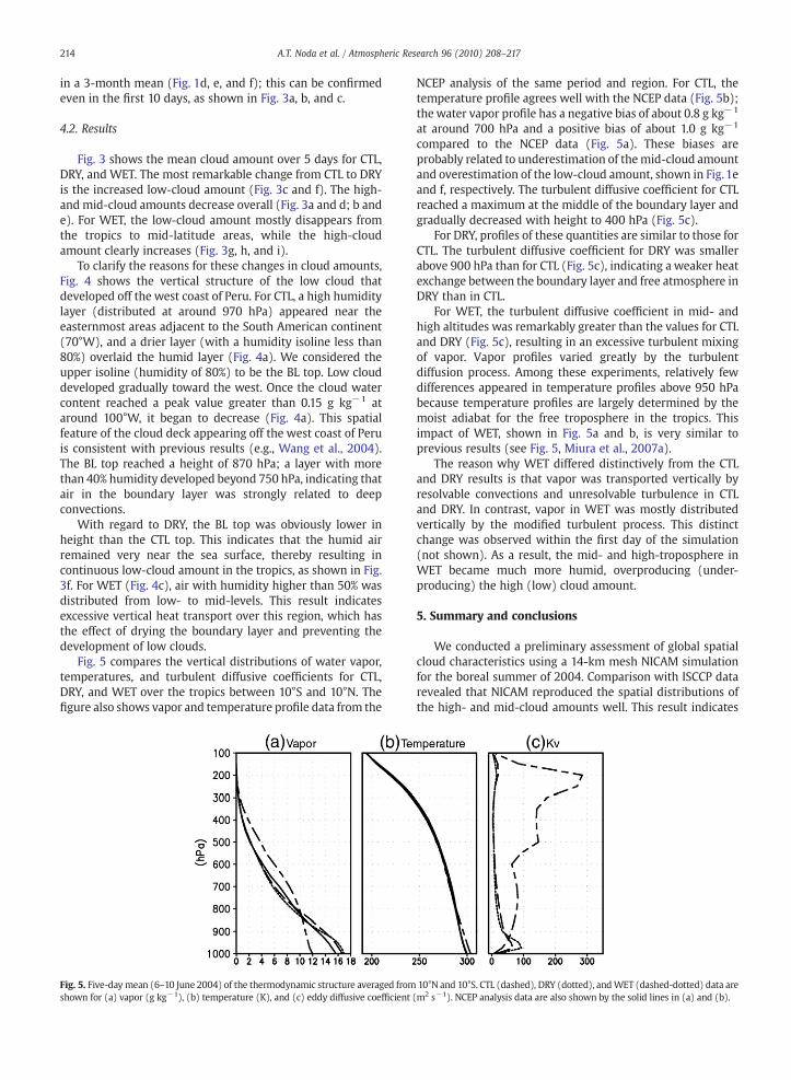
Fig. 5 compares the vertical distributions of water vapor,temperatures, and turbulent diffusive coefficients for CTL,DRY, and WET over the tropics between 10°S and 10°N. Thefigure also shows vapor and temperature profile data from the

Fig. 5. Five-daymean (6–10 June 2004) of the thermodynamic structure averaged fromshown for (a) vapor (g kg−1), (b) temperature (K), and (c) eddy diffusive coefficient

NCEP analysis of the same period and region. For CTL, thetemperature profile agrees well with the NCEP data (Fig. 5b);the water vapor profile has a negative bias of about 0.8 g kg−1

at around 700 hPa and a positive bias of about 1.0 g kg−1

compared to the NCEP data (Fig. 5a). These biases areprobably related to underestimation of themid-cloud amountand overestimation of the low-cloud amount, shown in Fig. 1eand f, respectively. The turbulent diffusive coefficient for CTLreached a maximum at the middle of the boundary layer andgradually decreased with height to 400 hPa (Fig. 5c).

For DRY, profiles of these quantities are similar to those forCTL. The turbulent diffusive coefficient for DRY was smallerabove 900 hPa than for CTL (Fig. 5c), indicating a weaker heatexchange between the boundary layer and free atmosphere inDRY than in CTL.

For WET, the turbulent diffusive coefficient in mid- andhigh altitudes was remarkably greater than the values for CTLand DRY (Fig. 5c), resulting in an excessive turbulent mixingof vapor. Vapor profiles varied greatly by the turbulentdiffusion process. Among these experiments, relatively fewdifferences appeared in temperature profiles above 950 hPabecause temperature profiles are largely determined by themoist adiabat for the free troposphere in the tropics. Thisimpact of WET, shown in Fig. 5a and b, is very similar toprevious results (see Fig. 5, Miura et al., 2007a).

The reason why WET differed distinctively from the CTLand DRY results is that vapor was transported vertically byresolvable convections and unresolvable turbulence in CTLand DRY. In contrast, vapor in WET was mostly distributedvertically by the modified turbulent process. This distinctchange was observed within the first day of the simulation(not shown). As a result, the mid- and high-troposphere inWET became much more humid, overproducing (under-producing) the high (low) cloud amount.

5. Summary and conclusions

We conducted a preliminary assessment of global spatialcloud characteristics using a 14-km mesh NICAM simulationfor the boreal summer of 2004. Comparison with ISCCP datarevealed that NICAM reproduced the spatial distributions ofthe high- and mid-cloud amounts well. This result indicates

10°N and 10°S. CTL (dashed), DRY (dotted), andWET (dashed-dotted) data are(m2 s−1). NCEP analysis data are also shown by the solid lines in (a) and (b).

215A.T. Noda et al. / Atmospheric Research 96 (2010) 208–217

that the horizontal resolution that we used was statisticallyable to capture deep convective clouds. Therefore, NICAM hasgreat potential, since it does not adopt the ad hoc tunings incloud parameterization used in conventional GCMs.

Our research differs most significantly from the researchpublished by Iga et al. (2007) in that we introduced the SGS-cloud effect into the TCM. This yielded great improvements inthe distribution of the low-cloud amounts, mainly in westernoffshore regions of subtropical continents. However, the bias inthe low-cloud amounts was much greater than that for thehigh- and mid-cloud amounts, resulting in overestimation ofOSR at the TOA. Uncertainty of small-scale and unresolvableeddies such as shallow convection is a continuing issue forGCRMs, as with conventional AGCMs (Bony and Dufresne,2005).

Our CTL experiment resulted in excessive low-cloudamount over almost the entire world. This bias in the low-cloud amount is opposite to that in many conventionalGCMs (e.g., Siebesma et al., 2004). In our experiment, theexcessive low-cloud amount was the consequence of thepositive humidity bias in the lower atmosphere. This moistbias was connected to the dry bias in the mid-troposphere,which also resulted in underestimated mid-cloud amount. Areason for such excessive low-cloud amount may be the lackof turbulent transport due to shallow cumulus convections.This is because level 2 of the M–Y model was constructedsupposing down-gradient turbulent diffusion. An additionaldevice to improve counter-gradient transport due toshallow cumulus convections would solve the bias and theexcessive cloud production in the tropical and subtropicalregions.

The lack of the entrainment mixing process accompanyingthe deep convective clouds may have been another cause ofthis dry bias, but this effect should not be explicitly resolvedunless the resolution is sufficiently fine, e.g., O(10 m). To thispoint, our experiments have not considered the effect ofentrainment mixing as subgrid-scale physics, though oursimulation was too coarse to resolve the entrainment mixingissue. An interesting issue for future study is thus to verify theturbulent mixing process that occurs near the edge and/or topof the deep clouds and the resultant heat redistribution in thetroposphere.

Our sensitivity experiments (Section 4) also revealed thatturbulent transport caused by SGS clouds is a key factorcontrolling GCRM cloud behavior. Large-eddy simulations withresolutions of O(10 m) will be required to resolve small-scaleconvections explicitly. Resolution of such small-scale convec-tion in global models will not be possible for some time, so it isimportant to examine in more detail the treatment of SGSclouds, even in the current generation of GCRMs.

Another issue is the combination of various physicalprocesses such as microphysics, turbulence, and radiation ina single SGS-cloud model. In this study, we simply assumedthat every grid cell was either totally clear or totally cloudyduring the radiation process. This assumption probablycaused the biases in OSR and OLR at the TOA: global averagevalues for the first 10 days increased by 0.6 Wm−2 and 0.3Wm−2, respectively (not shown). We did not utilize a fractionalcloud cover of SGS clouds (e.g., Eq. (11a)) to determine thecloud amount, and this resulted in overestimated low-cloudamount.

Recent use of high-resolution models that considerdetailed microphysics processes, together with explicitdynamic fields in large-eddy simulations (e.g., Stevens et al.,1998) has steadily contributed to the body of knowledgeabout cloud dynamics. Future studies can use these data toimprove the SGS scheme as well as the low-cloud amount inGCRMs.

Acknowledgments

We deeply appreciate the reviews for providing very usefulcomments on our original manuscript. We acknowledge theNICAMdevelopmentmembers for helpful discussions through-out this study. This work is partly supported by the InnovationProgram of Climate Projection for the 21st Century of theMinistry of Education, Culture, Sports, Science, and Technology(MEXT), Japan Grant-in-Aids for Scientific Research (B) (8)No.19740299 and (A) (5) No.19204046. The simulations of thisstudy were performed using the Earth Simulator.

Appendix A. Validation of the 5-day statistics

In Section 4, we analyzed the sensitivity of the turbulenttransport process to the global cloud distribution and thermalstructures using 5-day statistics. To validate the analyses, wealso investigated the time evolution of the simulated 10 daysfocusing particularly on the low-cloud amount together withthe temperature and vapor amounts.

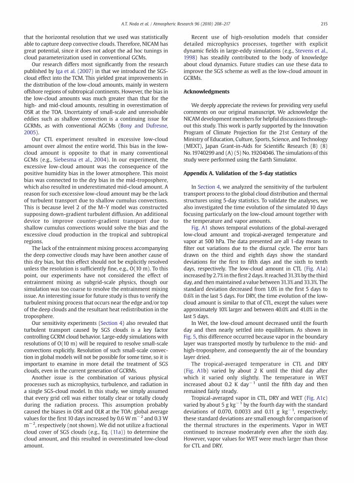
Fig. A1 shows temporal evolutions of the global-averagedlow-cloud amount and tropical-averaged temperature andvapor at 500 hPa. The data presented are all 1-day means tofilter out variations due to the diurnal cycle. The error barsdrawn on the third and eighth days show the standarddeviations for the first to fifth days and the sixth to tenthdays, respectively. The low-cloud amount in CTL (Fig. A1a)increased by 2.7% in thefirst 2 days. It reached31.3% by the thirdday, and thenmaintained a value between 31.3% and 33.3%. Thestandard deviation decreased from 1.0% in the first 5 days to0.6% in the last 5 days. For DRY, the time evolution of the low-cloud amount is similar to that of CTL, except the values wereapproximately 10% larger and between 40.0% and 41.0% in thelast 5 days.

In Wet, the low-cloud amount decreased until the fourthday and then nearly settled into equilibrium. As shown inFig. 5, this difference occurred because vapor in the boundarylayer was transported mostly by turbulence to the mid- andhigh-troposphere, and consequently the air of the boundarylayer dried.

The tropical-averaged temperature in CTL and DRY(Fig. A1b) varied by about 2 K until the third day afterwhich it varied only slightly. The temperature in WETincreased about 0.2 K day−1 until the fifth day and thenremained fairly steady.

Tropical-averaged vapor in CTL, DRY and WET (Fig. A1c)varied by about 5 g kg−1 by the fourth day with the standarddeviations of 0.070, 0.0033 and 0.11 g kg−1, respectively;these standard deviations are small enough for comparison ofthe thermal structures in the experiments. Vapor in WETcontinued to increase moderately even after the sixth day.However, vapor values for WET were much larger than thosefor CTL and DRY.

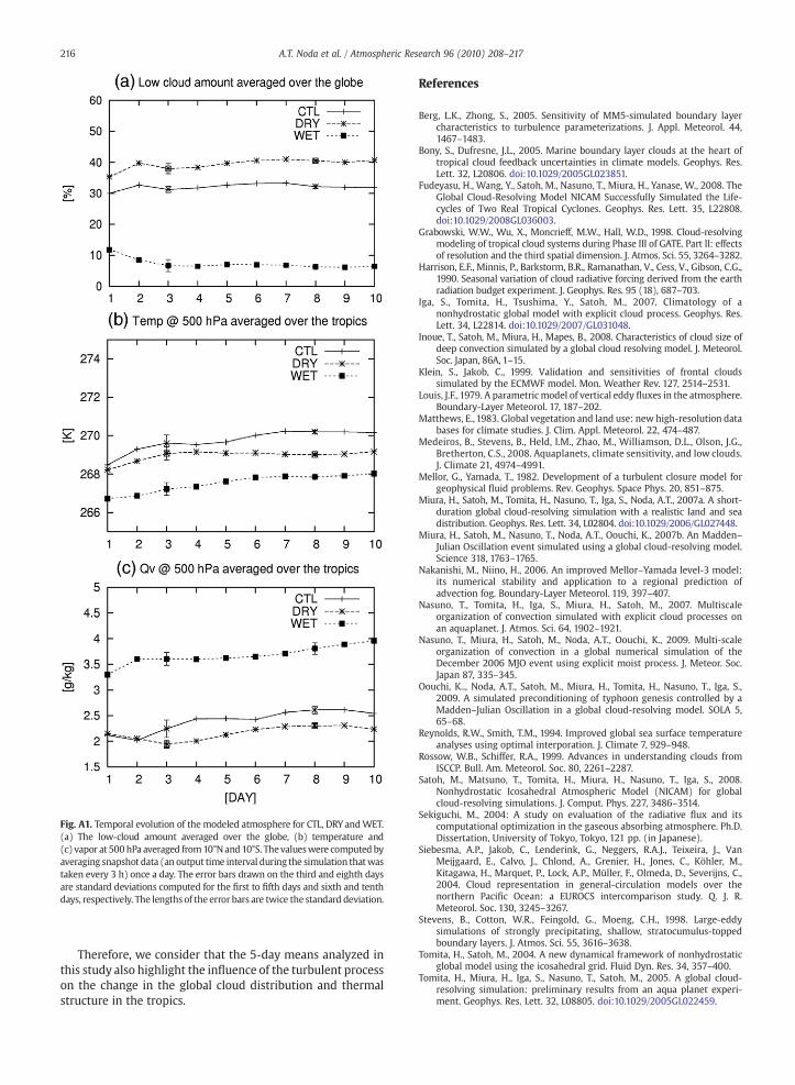
Fig. A1. Temporal evolution of the modeled atmosphere for CTL, DRY andWET.(a) The low-cloud amount averaged over the globe, (b) temperature and(c) vapor at 500 hPa averaged from10°Nand10°S. Thevalueswere computed byaveraging snapshot data (an output time interval during the simulation thatwastaken every 3 h) once a day. The error bars drawn on the third and eighth daysare standard deviations computed for the first to fifth days and sixth and tenthdays, respectively. The lengths of the error bars are twice the standard deviation.

216 A.T. Noda et al. / Atmospheric Research 96 (2010) 208–217

Therefore, we consider that the 5-day means analyzed inthis study also highlight the influence of the turbulent processon the change in the global cloud distribution and thermalstructure in the tropics.

References

Berg, L.K., Zhong, S., 2005. Sensitivity of MM5-simulated boundary layercharacteristics to turbulence parameterizations. J. Appl. Meteorol. 44,1467–1483.

Bony, S., Dufresne, J.L., 2005. Marine boundary layer clouds at the heart oftropical cloud feedback uncertainties in climate models. Geophys. Res.Lett. 32, L20806. doi:10.1029/2005GL023851.

Fudeyasu, H., Wang, Y., Satoh, M., Nasuno, T., Miura, H., Yanase, W., 2008. TheGlobal Cloud-Resolving Model NICAM Successfully Simulated the Life-cycles of Two Real Tropical Cyclones. Geophys. Res. Lett. 35, L22808.doi:10.1029/2008GL036003.

Grabowski, W.W., Wu, X., Moncrieff, M.W., Hall, W.D., 1998. Cloud-resolvingmodeling of tropical cloud systems during Phase III of GATE. Part II: effectsof resolution and the third spatial dimension. J. Atmos. Sci. 55, 3264–3282.

Harrison, E.F., Minnis, P., Barkstorm, B.R., Ramanathan, V., Cess, V., Gibson, C.G.,1990. Seasonal variation of cloud radiative forcing derived from the earthradiation budget experiment. J. Geophys. Res. 95 (18), 687–703.

Iga, S., Tomita, H., Tsushima, Y., Satoh, M., 2007. Climatology of anonhydrostatic global model with explicit cloud process. Geophys. Res.Lett. 34, L22814. doi:10.1029/2007/GL031048.

Inoue, T., Satoh, M., Miura, H., Mapes, B., 2008. Characteristics of cloud size ofdeep convection simulated by a global cloud resolving model. J. Meteorol.Soc. Japan, 86A, 1–15.

Klein, S., Jakob, C., 1999. Validation and sensitivities of frontal cloudssimulated by the ECMWF model. Mon. Weather Rev. 127, 2514–2531.

Louis, J.F., 1979. A parametricmodel of vertical eddy fluxes in the atmosphere.Boundary-Layer Meteorol. 17, 187–202.

Matthews, E., 1983. Global vegetation and land use: new high-resolution databases for climate studies. J. Clim. Appl. Meteorol. 22, 474–487.

Medeiros, B., Stevens, B., Held, I.M., Zhao, M., Williamson, D.L., Olson, J.G.,Bretherton, C.S., 2008. Aquaplanets, climate sensitivity, and low clouds.J. Climate 21, 4974–4991.

Mellor, G., Yamada, T., 1982. Development of a turbulent closure model forgeophysical fluid problems. Rev. Geophys. Space Phys. 20, 851–875.

Miura, H., Satoh, M., Tomita, H., Nasuno, T., Iga, S., Noda, A.T., 2007a. A short-duration global cloud-resolving simulation with a realistic land and seadistribution. Geophys. Res. Lett. 34, L02804. doi:10.1029/2006/GL027448.

Miura, H., Satoh, M., Nasuno, T., Noda, A.T., Oouchi, K., 2007b. An Madden–Julian Oscillation event simulated using a global cloud-resolving model.Science 318, 1763–1765.

Nakanishi, M., Niino, H., 2006. An improved Mellor–Yamada level-3 model:its numerical stability and application to a regional prediction ofadvection fog. Boundary-Layer Meteorol. 119, 397–407.

Nasuno, T., Tomita, H., Iga, S., Miura, H., Satoh, M., 2007. Multiscaleorganization of convection simulated with explicit cloud processes onan aquaplanet. J. Atmos. Sci. 64, 1902–1921.

Nasuno, T., Miura, H., Satoh, M., Noda, A.T., Oouchi, K., 2009. Multi-scaleorganization of convection in a global numerical simulation of theDecember 2006 MJO event using explicit moist process. J. Meteor. Soc.Japan 87, 335–345.

Oouchi, K.., Noda, A.T., Satoh, M., Miura, H., Tomita, H., Nasuno, T., Iga, S.,2009. A simulated preconditioning of typhoon genesis controlled by aMadden–Julian Oscillation in a global cloud-resolving model. SOLA 5,65–68.

Reynolds, R.W., Smith, T.M., 1994. Improved global sea surface temperatureanalyses using optimal interporation. J. Climate 7, 929–948.

Rossow, W.B., Schiffer, R.A., 1999. Advances in understanding clouds fromISCCP. Bull. Am. Meteorol. Soc. 80, 2261–2287.

Satoh, M., Matsuno, T., Tomita, H., Miura, H., Nasuno, T., Iga, S., 2008.Nonhydrostatic Icosahedral Atmospheric Model (NICAM) for globalcloud-resolving simulations. J. Comput. Phys. 227, 3486–3514.

Sekiguchi, M., 2004: A study on evaluation of the radiative flux and itscomputational optimization in the gaseous absorbing atmosphere. Ph.D.Dissertation, University of Tokyo, Tokyo, 121 pp. (in Japanese).

Siebesma, A.P., Jakob, C., Lenderink, G., Neggers, R.A.J., Teixeira, J., VanMeijgaard, E., Calvo, J., Chlond, A., Grenier, H., Jones, C., Köhler, M.,Kitagawa, H., Marquet, P., Lock, A.P., Müller, F., Olmeda, D., Severijns, C.,2004. Cloud representation in general-circulation models over thenorthern Pacific Ocean: a EUROCS intercomparison study. Q. J. R.Meteorol. Soc. 130, 3245–3267.

Stevens, B., Cotton, W.R., Feingold, G., Moeng, C.H., 1998. Large-eddysimulations of strongly precipitating, shallow, stratocumulus-toppedboundary layers. J. Atmos. Sci. 55, 3616–3638.

Tomita, H., Satoh, M., 2004. A new dynamical framework of nonhydrostaticglobal model using the icosahedral grid. Fluid Dyn. Res. 34, 357–400.

Tomita, H., Miura, H., Iga, S., Nasuno, T., Satoh, M., 2005. A global cloud-resolving simulation: preliminary results from an aqua planet experi-ment. Geophys. Res. Lett. 32, L08805. doi:10.1029/2005GL022459.

217A.T. Noda et al. / Atmospheric Research 96 (2010) 208–217

Wang, Y., Xie, S.P., Xu, H., Wang, B., 2004. Regional model simulations ofmarine boundary layer clouds over the southeast pacific off SouthAmerica. Part I: control experiment. Mon. Weather Rev. 132, 274–296.

Webb, M., Senior, C., Bony, S., Morcrette, J.J., 2001. Combining ERBE and ISCCPdata to assess clouds in the Hadley Centre, ECMWF and LMD atmosphericclimate models. J. Clim. Dyn. 17, 905–922.

Zhang, M.H., Lin, W.Y., Klein, S.A., Bacmeister, J.T., Bony, S., Cederwall, R.T., DelGenio, A.D., Hack, J.J., Loeb, N.G., Lohmann, U., Minnis, P., Musat, I., Pincus,

R., Stier, P., Suarez, M.J., Webb, M.J., Wu, J.B., Xie, S.C., Yao, M.S., Zhang, J.H.,2005. Comparing clouds and their seasonal variations in 10 atmosphericgeneral circulation models with satellite measurements. J. Geophys. Res.110, D15S02. doi:10.1029/2004JD005021.

Zhong, S., In, H., Clements, C., 2007. Impact of turbulence, land surface, andradiationparameterizationonsimulatedboundary layerproperties inacoastalenvironment. J. Geophys. Res. 112, D13110. doi:10.1029/2006JD008274.