Implementing H1 by Resolution

Implementing H1 by Resolution ∗

Jean Goubault-Larrecq ([email protected])LSV/UMR 8643, CNRS & ENS Cachan; INRIA Futurs projet SECSI

Abstract. The h1 tool is an implementation of a theorem prover dedicated tosolving Nielson, Nielson and Seidl’s decidable class H1 of first-order Horn clauses.This is based on ordered resolution with selection, eager ε-splitting—a special case ofRiazanov and Voronkov’s splitting with naming rule—, and several additional rules.We tested h1 on a few examples coming from cryptographic protocol verification,and in particular some produced by the csur static code analyzer, due to Parrennesand the author, a tool to detect leakage of secrets in C programs. We also testedh1 on a collection of about 800 problems without equality originating from Sutcliffeand Suttner’s TPTP library. We use these examples and report on the efficiencyof h1. Particularly, we investigate the merits of several optimizations built into h1,which appear to be new. In each case, we try to understand why they fare well orfail. These include naive static soft typing, on-the-fly abbreviation of deep terms,and detecting fully-defined predicates. Of the latter three, on-the-fly abbreviation ofdeep terms, a variant of the rule of definition introduction known in Prolog programtransformation circles, offers drastic speedups in specific applications.

Keywords: resolution, splitting, H1, Horn clauses, abstract interpretation, staticsoft typing, abbreviation, definition introduction, TPTP, cryptographic protocolverification

∗ Partially supported by the ACI Rossignol, and the RNTL projects EVA andPROUVE.

c© 2005 Kluwer Academic Publishers. Printed in the Netherlands.

implem.tex; 13/12/2005; 16:22; p.1

Keywords: resolution, splitting, H1, Horn clauses, abstract interpretation, staticsoft typing, abbreviation, definition introduction, TPTP, cryptographic protocolverification

1. Introduction

Nielson, Nielson and Seidl [16] introduced the class H1 of first-orderHorn clause sets to model reachability in the spi-calculus. They showedthat H1 satisfiability is decidable and DEXPTIME-complete, and thatH1 clause sets can be converted to equivalent tree automata in expo-nential time—so H1 defines regular tree languages. Further subclassesof H1, in particular H3, have polynomial time complexity.

This was further refined in [9], where it was shown that H1 couldbe decided by fairly standard automated deduction techniques, withoptimal complexity, that is, in no more than deterministic exponentialtime. The basic rule is ordered resolution with selection [2], with asuitable ordering and a suitable selection function, supplemented by aform of Riazanov and Voronkov’s splitting with naming rule [18].

While this would seem to indicate that off-the-shelf resolution proverscould be used to decide H1, the ones that we tested resisted using theparticular selection function that is required here. On the other hand,it is an interesting question in itself whether the particular form of H1

clauses lends itself to more efficient proof procedures.This prompted the initial impetus to implement a dedicated res-

olution prover for the H1 class. The resulting tool, called h1, wasimplemented and optimized by the author during the years 2003–2004.Some of the lessons learned indeed apply specifically to H1, but someof the optimizations we found to be most useful are likely to find ap-plication in more general situations as well. In this paper, we wish toreport on the experience we gained during this effort.

1.1. A word on methodology.

When some implementation effort such as h1 is initiated by an aca-demic researcher, there is always some confusion as to what the goalsof this effort should be. You may want to understand whether someoptimization or some deduction rule is useful, and why; or you maystrive for, say, the fastest prover you can. Hooker [12] observes that,

c© 2005 Kluwer Academic Publishers. Printed in the Netherlands.

implem.tex; 13/12/2005; 16:22; p.2

3

while the former is probably the most useful to science, the latter iswhat most researchers attempt to do.

The second approach is what Hooker calls competitive testing : spendsome time implementing, optimizing, tuning your code, then compare itagainst other state-of-the-art provers, e.g., by entering some well-knowncompetition such as the yearly CASC, held at the CADE and IJCARconferences. Hooker observes that this is essentially useless from thepoint of view of the advancement of science. You may have won, thismay be because of some particularly clever algorithm, or because youare a particularly skillful programmer (what is the part of each?). Youmay have won because the particular blend of rules and optimizationsyou used is indeed efficient. In each case, winning a competition doesnot explain why a particular algorithm, rule, or optimization has anybenefit, and in which situations.

The first approach is based on controlled experimentation, see Hooker(op.cit.). This is the age-old principle at the root of scientific experimen-tation. The intent is that you run experiments not to boast about yourparticular algorithm, but to confirm or refute hypotheses. E.g., Hookerexemplifies this approach by showing how a controlled experiment couldstate which of the following hypothesis were likely to explain the effi-ciency of branching rules in Davis-Putnam-like SAT solvers: a) betterbranching rules try to maximize the probability that subproblems aresatisfiable, and b) better branching rules simplify the subproblems asmuch as possible. Hooker claims that predictions following from hy-pothesis a) were consistenly refuted by experiment, so that hypothesisa) had to be abandoned.

We largely agree with Hooker. Nonetheless, we still made the ini-tial mistake of trying to get the most efficient algorithm possible todecide H1. The h1 tool was, in our opinion, rather successful from thispoint of view. During 2003-2004, we concentrated on a few (about 20)problems coming from the application domain we were interested in,cryptographic protocol verification, and specifically, verification thatsensitive data remained confidential in C programs [11]. We describethe most prominent examples below. A few weeks before we submittedthis paper, we decided that it would be natural to deal with exam-ples coming from the now well-established TPTP collection [20]. Morespecifically, the H1 clause sets we picked to test h1 were:

− Five among the problems coming from cryptographic protocol ver-ification, which were relatively or even extremely challenging atsome steps of the development of h1. We call them the Parrennes

examples, since they were communicated to us by Fabrice Par-rennes. The examples alice full1.h1.p, alice full2.h1.p, and

implem.tex; 13/12/2005; 16:22; p.3

4

alice full3.h1.p that we shall repeatedly refer to later wereproduced by an early implementation of csur, our C code analyzer[11]. The latter files are in fact not in H1, but they are close. Thereis a standard approximation procedure (see Section 3.2 below) thatconverts any first-order clause set S without equality to an H1

clause set S0 that over-approximates it, meaning in particular thatif S0 is satisfiable then so is S, and the least Herbrand model ofS0 (which can be presented as a regular tree language) is a modelof S.

The files we consider here have gone through this approximationprocedure after being generated by csur. The early implementa-tion of csur we used contained some bugs which, interestingly,generated relatively hard H1 clause sets. (As the names indicatepartly, the examples cited above encode Alice’s role in a workingC implementation of the Needham-Schroeder public-key protocol[15]. The first too are unsatisfiable—there is an attack—, the thirdone is satisfiable—no attack.)

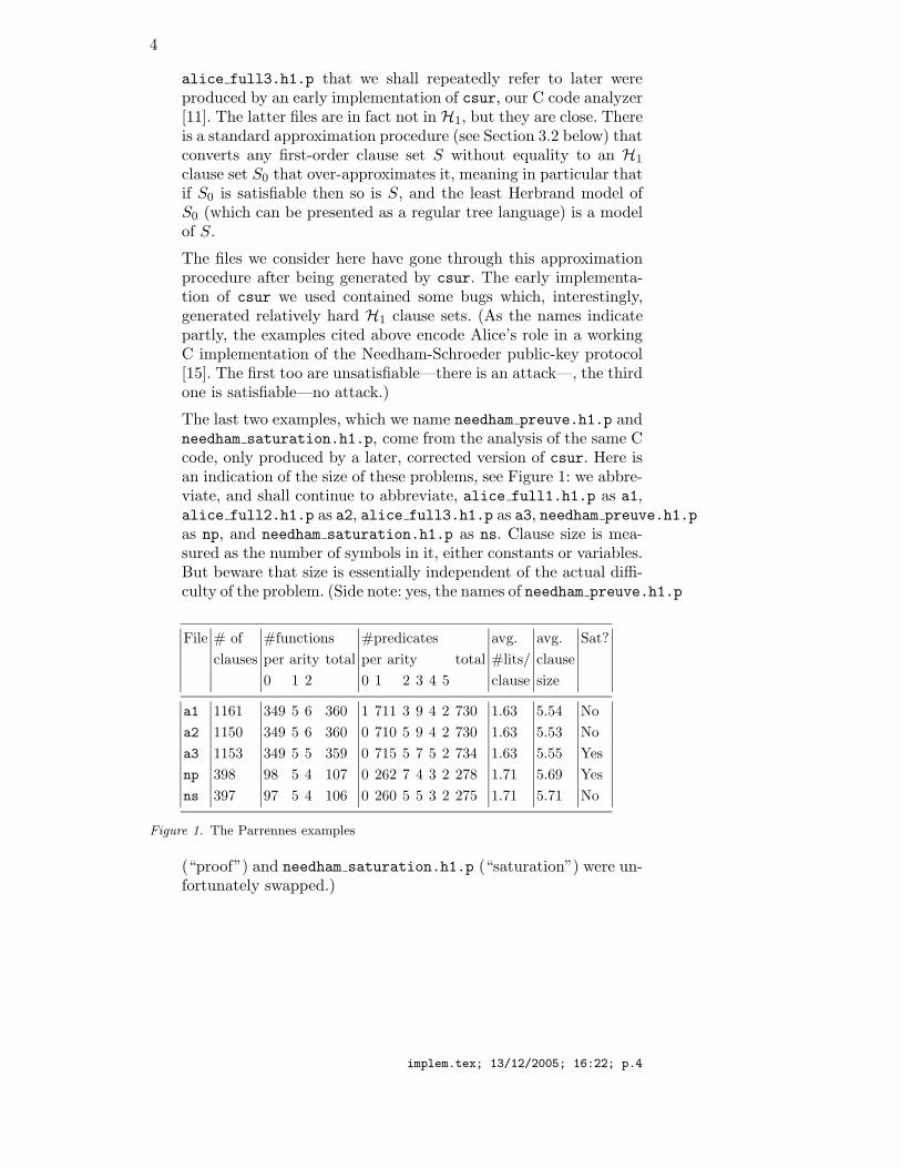
The last two examples, which we name needham preuve.h1.p andneedham saturation.h1.p, come from the analysis of the same Ccode, only produced by a later, corrected version of csur. Here isan indication of the size of these problems, see Figure 1: we abbre-viate, and shall continue to abbreviate, alice full1.h1.p as a1,alice full2.h1.p as a2, alice full3.h1.p as a3, needham preuve.h1.p

as np, and needham saturation.h1.p as ns. Clause size is mea-sured as the number of symbols in it, either constants or variables.But beware that size is essentially independent of the actual diffi-culty of the problem. (Side note: yes, the names of needham preuve.h1.p

File # of #functions #predicates avg. avg. Sat?

clauses per arity total per arity total #lits/ clause

0 1 2 0 1 2 3 4 5 clause size

a1 1161 349 5 6 360 1 711 3 9 4 2 730 1.63 5.54 No

a2 1150 349 5 6 360 0 710 5 9 4 2 730 1.63 5.53 No

a3 1153 349 5 5 359 0 715 5 7 5 2 734 1.63 5.55 Yes

np 398 98 5 4 107 0 262 7 4 3 2 278 1.71 5.69 Yes

ns 397 97 5 4 106 0 260 5 5 3 2 275 1.71 5.71 No

Figure 1. The Parrennes examples

(“proof”) and needham saturation.h1.p (“saturation”) were un-fortunately swapped.)

implem.tex; 13/12/2005; 16:22; p.4

5

− 808 problems extracted from the TPTP library, version 3.0.1 [20].Almost none of the problems from the TPTP library are in the H1

class: only 2 from the COM category (COM001-1.p and COM002-1.p),1 from KRS (KRS004-1.p), 1 from MGT (MGT036-3.p), 1 from MSC

(MSC005-1.p), and 10 from PUZ, totalling 15.

To compensate, we again used the approximation procedure in-dicated above. We selected those problems without equality fromthe COM (computation theory), FLD (fields), KRS (knowledge rep-resentation systems), LCL (logic calculi), MGT (management, or-ganization theory), MSC (miscellaneous), NLP (natural languageprocessing), and PUZ (puzzles). We ignored the other categories,which rest heavily on equality. Finding problems without equalitywas done by executing the Unix command grep -l ’ 0 equa’,profiting from the fact that each TPTP file comes with extensivedescriptions of its properties.

1.2. A Word on Precision

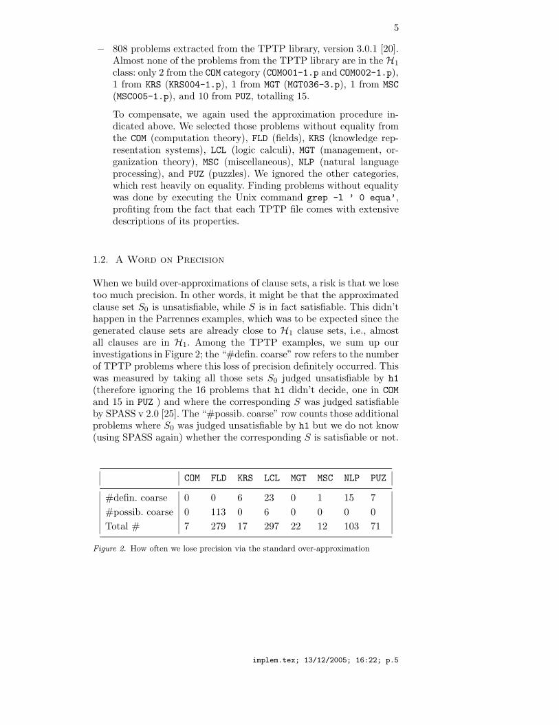
When we build over-approximations of clause sets, a risk is that we losetoo much precision. In other words, it might be that the approximatedclause set S0 is unsatisfiable, while S is in fact satisfiable. This didn’thappen in the Parrennes examples, which was to be expected since thegenerated clause sets are already close to H1 clause sets, i.e., almostall clauses are in H1. Among the TPTP examples, we sum up ourinvestigations in Figure 2; the “#defin. coarse” row refers to the numberof TPTP problems where this loss of precision definitely occurred. Thiswas measured by taking all those sets S0 judged unsatisfiable by h1

(therefore ignoring the 16 problems that h1 didn’t decide, one in COM

and 15 in PUZ ) and where the corresponding S was judged satisfiableby SPASS v 2.0 [25]. The “#possib. coarse” row counts those additionalproblems where S0 was judged unsatisfiable by h1 but we do not know(using SPASS again) whether the corresponding S is satisfiable or not.

COM FLD KRS LCL MGT MSC NLP PUZ

#defin. coarse 0 0 6 23 0 1 15 7

#possib. coarse 0 113 0 6 0 0 0 0

Total # 7 279 17 297 22 12 103 71

Figure 2. How often we lose precision via the standard over-approximation

implem.tex; 13/12/2005; 16:22; p.5

6

1.3. Competitive Testing

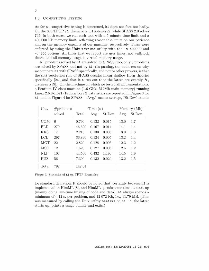
As far as competitive testing is concerned, h1 does not fare too badly.On the 808 TPTP H1 clause sets, h1 solves 792, while SPASS 2.0 solves795. In both cases, we ran each tool with a 5 minute time limit and a400 000 Kb memory limit, reflecting reasonable limits on our patienceand on the memory capacity of our machine, respectively. These wereenforced by using the Unix memtime utility with the -m 400000 and-c 300 options. All times that we report are user times, not wallclocktimes, and all memory usage is virtual memory usage.

All problems solved by h1 are solved by SPASS, too; only 3 problemsare solved by SPASS and not by h1. (In passing, the main reason whywe compare h1 with SPASS specifically, and not to other provers, is thatthe sort resolution rule of SPASS decides linear shallow Horn theoriesspecifically [24], and that it turns out that the latter are exactly H1

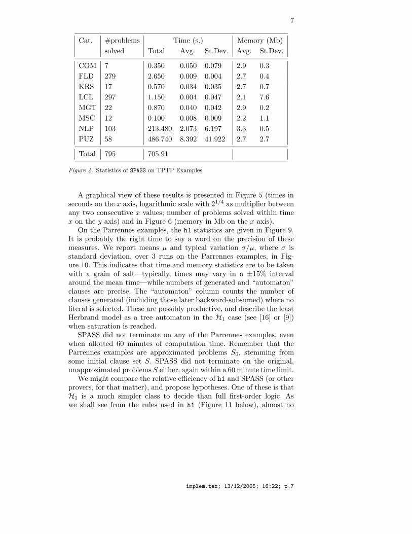
clause sets [9].) On the machine on which we tested all implementations,a Pentium IV class machine (1.6 GHz, 512Mb main memory) runningLinux 2.6.8-1.521 (Fedora Core 2), statistics are reported in Figure 3 forh1, and in Figure 4 for SPASS. “Avg.” means average, “St.Dev” stands

Cat. #problems Time (s.) Memory (Mb)

solved Total Avg. St.Dev. Avg. St.Dev.

COM 6 0.790 0.132 0.015 13.0 1.7

FLD 279 46.520 0.167 0.014 14.1 1.4

KRS 17 2.210 0.130 0.008 13.0 1.3

LCL 297 36.890 0.124 0.005 13.2 1.4

MGT 22 2.820 0.128 0.005 12.3 1.2

MSC 12 1.520 0.127 0.006 12.5 1.2

NLP 103 44.500 0.432 1.190 14.5 1.9

PUZ 56 7.390 0.132 0.020 13.2 1.5

Total 792 142.64

Figure 3. Statistics of h1 on TPTP Examples

for standard deviation. It should be noted that, certainly because h1 isimplemented in HimML [8], and HimML spends some time at start-up(mainly doing run-time linking of code and data), h1 always spends aminimum of 0.12 s. per problem, and 12 072 Kb, i.e., 11.79 MB. (Thiswas measured by calling the Unix utility memtime on h1 -h; the latterstarts up, prints a usage banner and exits.)

implem.tex; 13/12/2005; 16:22; p.6

7



COM 7 0.350 0.050 0.079 2.9 0.3

FLD 279 2.650 0.009 0.004 2.7 0.4

KRS 17 0.570 0.034 0.035 2.7 0.7

LCL 297 1.150 0.004 0.047 2.1 7.6

MGT 22 0.870 0.040 0.042 2.9 0.2

MSC 12 0.100 0.008 0.009 2.2 1.1

NLP 103 213.480 2.073 6.197 3.3 0.5

PUZ 58 486.740 8.392 41.922 2.7 2.7

Total 795 705.91

Figure 4. Statistics of SPASS on TPTP Examples

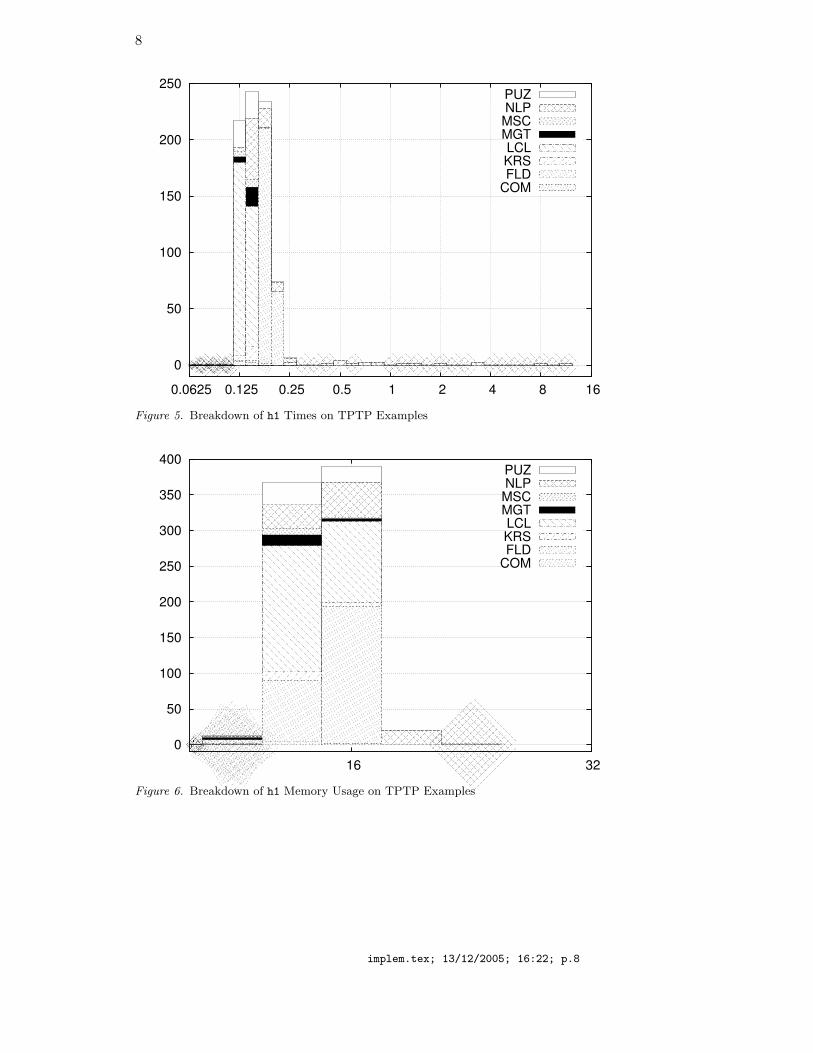
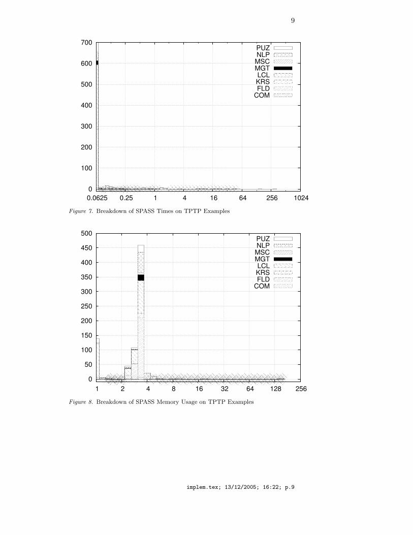
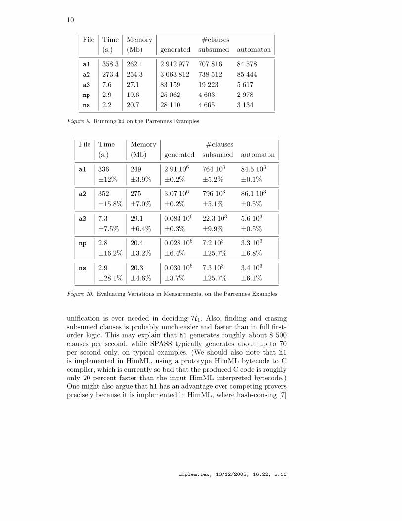
A graphical view of these results is presented in Figure 5 (times inseconds on the x axis, logarithmic scale with 21/4 as multiplier betweenany two consecutive x values; number of problems solved within timex on the y axis) and in Figure 6 (memory in Mb on the x axis).

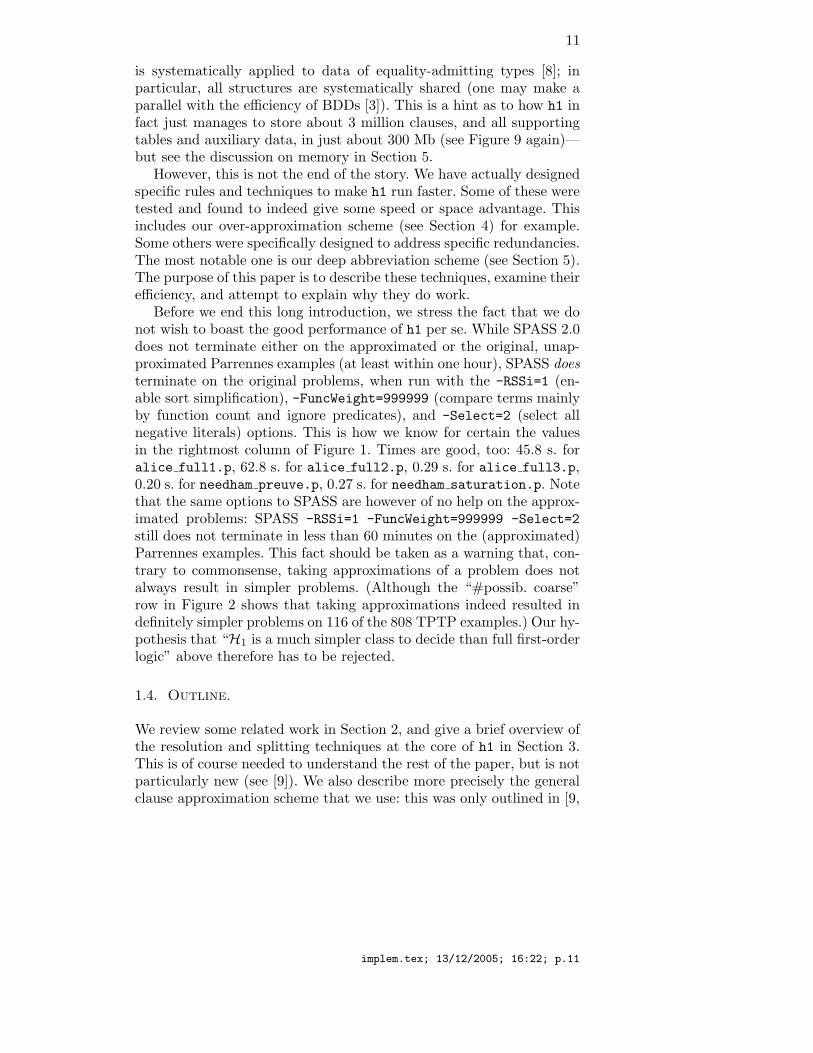
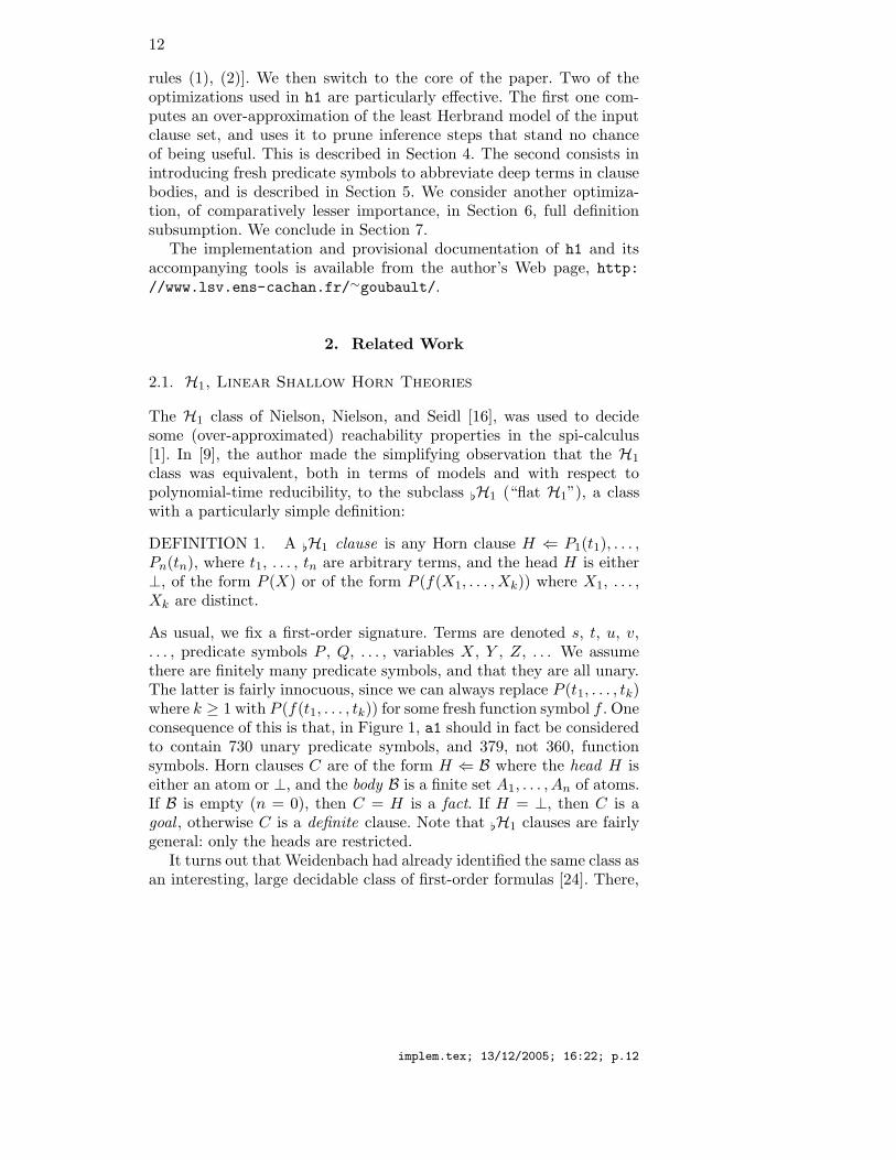
On the Parrennes examples, the h1 statistics are given in Figure 9.It is probably the right time to say a word on the precision of thesemeasures. We report means µ and typical variation σ/µ, where σ isstandard deviation, over 3 runs on the Parrennes examples, in Fig-ure 10. This indicates that time and memory statistics are to be takenwith a grain of salt—typically, times may vary in a ±15% intervalaround the mean time—while numbers of generated and “automaton”clauses are precise. The “automaton” column counts the number ofclauses generated (including those later backward-subsumed) where noliteral is selected. These are possibly productive, and describe the leastHerbrand model as a tree automaton in the H1 case (see [16] or [9])when saturation is reached.

SPASS did not terminate on any of the Parrennes examples, evenwhen allotted 60 minutes of computation time. Remember that theParrennes examples are approximated problems S0, stemming fromsome initial clause set S. SPASS did not terminate on the original,unapproximated problems S either, again within a 60 minute time limit.

We might compare the relative efficiency of h1 and SPASS (or otherprovers, for that matter), and propose hypotheses. One of these is thatH1 is a much simpler class to decide than full first-order logic. Aswe shall see from the rules used in h1 (Figure 11 below), almost no

implem.tex; 13/12/2005; 16:22; p.7

8

0

50

100

150

200

250

0.0625 0.125 0.25 0.5 1 2 4 8 16

PUZNLPMSCMGTLCLKRSFLD

COM

Figure 5. Breakdown of h1 Times on TPTP Examples

0

50

100

150

200

250

300

350

400

16 32


COM

Figure 6. Breakdown of h1 Memory Usage on TPTP Examples

implem.tex; 13/12/2005; 16:22; p.8

9

0

100

200

300

400

500

600

700

0.0625 0.25 1 4 16 64 256 1024


COM

Figure 7. Breakdown of SPASS Times on TPTP Examples

0

50

100

150

200

250

300

350

400

450

500

1 2 4 8 16 32 64 128 256


COM

Figure 8. Breakdown of SPASS Memory Usage on TPTP Examples

implem.tex; 13/12/2005; 16:22; p.9

10

File Time Memory #clauses

(s.) (Mb) generated subsumed automaton

a1 358.3 262.1 2 912 977 707 816 84 578

a2 273.4 254.3 3 063 812 738 512 85 444

a3 7.6 27.1 83 159 19 223 5 617

np 2.9 19.6 25 062 4 603 2 978

ns 2.2 20.7 28 110 4 665 3 134

Figure 9. Running h1 on the Parrennes Examples



a1 336 249 2.91 106 764 103 84.5 103

±12% ±3.9% ±0.2% ±5.2% ±0.1%

a2 352 275 3.07 106 796 103 86.1 103

±15.8% ±7.0% ±0.2% ±5.1% ±0.5%

a3 7.3 29.1 0.083 106 22.3 103 5.6 103

±7.5% ±6.4% ±0.3% ±9.9% ±0.5%

np 2.8 20.4 0.028 106 7.2 103 3.3 103

±16.2% ±3.2% ±6.4% ±25.7% ±6.8%

ns 2.9 20.3 0.030 106 7.3 103 3.4 103

±28.1% ±4.6% ±3.7% ±25.7% ±6.1%

Figure 10. Evaluating Variations in Measurements, on the Parrennes Examples

unification is ever needed in deciding H1. Also, finding and erasingsubsumed clauses is probably much easier and faster than in full first-order logic. This may explain that h1 generates roughly about 8 500clauses per second, while SPASS typically generates about up to 70per second only, on typical examples. (We should also note that h1

is implemented in HimML, using a prototype HimML bytecode to Ccompiler, which is currently so bad that the produced C code is roughlyonly 20 percent faster than the input HimML interpreted bytecode.)One might also argue that h1 has an advantage over competing proversprecisely because it is implemented in HimML, where hash-consing [7]

implem.tex; 13/12/2005; 16:22; p.10

11

is systematically applied to data of equality-admitting types [8]; inparticular, all structures are systematically shared (one may make aparallel with the efficiency of BDDs [3]). This is a hint as to how h1 infact just manages to store about 3 million clauses, and all supportingtables and auxiliary data, in just about 300 Mb (see Figure 9 again)—but see the discussion on memory in Section 5.

However, this is not the end of the story. We have actually designedspecific rules and techniques to make h1 run faster. Some of these weretested and found to indeed give some speed or space advantage. Thisincludes our over-approximation scheme (see Section 4) for example.Some others were specifically designed to address specific redundancies.The most notable one is our deep abbreviation scheme (see Section 5).The purpose of this paper is to describe these techniques, examine theirefficiency, and attempt to explain why they do work.

Before we end this long introduction, we stress the fact that we donot wish to boast the good performance of h1 per se. While SPASS 2.0does not terminate either on the approximated or the original, unap-proximated Parrennes examples (at least within one hour), SPASS does

terminate on the original problems, when run with the -RSSi=1 (en-able sort simplification), -FuncWeight=999999 (compare terms mainlyby function count and ignore predicates), and -Select=2 (select allnegative literals) options. This is how we know for certain the valuesin the rightmost column of Figure 1. Times are good, too: 45.8 s. foralice full1.p, 62.8 s. for alice full2.p, 0.29 s. for alice full3.p,0.20 s. for needham preuve.p, 0.27 s. for needham saturation.p. Notethat the same options to SPASS are however of no help on the approx-imated problems: SPASS -RSSi=1 -FuncWeight=999999 -Select=2

still does not terminate in less than 60 minutes on the (approximated)Parrennes examples. This fact should be taken as a warning that, con-trary to commonsense, taking approximations of a problem does notalways result in simpler problems. (Although the “#possib. coarse”row in Figure 2 shows that taking approximations indeed resulted indefinitely simpler problems on 116 of the 808 TPTP examples.) Our hy-pothesis that “H1 is a much simpler class to decide than full first-orderlogic” above therefore has to be rejected.

1.4. Outline.

We review some related work in Section 2, and give a brief overview ofthe resolution and splitting techniques at the core of h1 in Section 3.This is of course needed to understand the rest of the paper, but is notparticularly new (see [9]). We also describe more precisely the generalclause approximation scheme that we use: this was only outlined in [9,

implem.tex; 13/12/2005; 16:22; p.11

12

rules (1), (2)]. We then switch to the core of the paper. Two of theoptimizations used in h1 are particularly effective. The first one com-putes an over-approximation of the least Herbrand model of the inputclause set, and uses it to prune inference steps that stand no chanceof being useful. This is described in Section 4. The second consists inintroducing fresh predicate symbols to abbreviate deep terms in clausebodies, and is described in Section 5. We consider another optimiza-tion, of comparatively lesser importance, in Section 6, full definitionsubsumption. We conclude in Section 7.

The implementation and provisional documentation of h1 and itsaccompanying tools is available from the author’s Web page, http://www.lsv.ens-cachan.fr/∼goubault/.

2. Related Work

2.1. H1, Linear Shallow Horn Theories

The H1 class of Nielson, Nielson, and Seidl [16], was used to decidesome (over-approximated) reachability properties in the spi-calculus[1]. In [9], the author made the simplifying observation that the H1

class was equivalent, both in terms of models and with respect topolynomial-time reducibility, to the subclass [H1 (“flat H1”), a classwith a particularly simple definition:

DEFINITION 1. A [H1 clause is any Horn clause H ⇐ P1(t1), . . . ,Pn(tn), where t1, . . . , tn are arbitrary terms, and the head H is either⊥, of the form P (X) or of the form P (f(X1, . . . ,Xk)) where X1, . . . ,Xk are distinct.

As usual, we fix a first-order signature. Terms are denoted s, t, u, v,. . . , predicate symbols P , Q, . . . , variables X, Y , Z, . . . We assumethere are finitely many predicate symbols, and that they are all unary.The latter is fairly innocuous, since we can always replace P (t1, . . . , tk)where k ≥ 1 with P (f(t1, . . . , tk)) for some fresh function symbol f . Oneconsequence of this is that, in Figure 1, a1 should in fact be consideredto contain 730 unary predicate symbols, and 379, not 360, functionsymbols. Horn clauses C are of the form H ⇐ B where the head H iseither an atom or ⊥, and the body B is a finite set A1, . . . , An of atoms.If B is empty (n = 0), then C = H is a fact. If H = ⊥, then C is agoal , otherwise C is a definite clause. Note that [H1 clauses are fairlygeneral: only the heads are restricted.

It turns out that Weidenbach had already identified the same class asan interesting, large decidable class of first-order formulas [24]. There,

implem.tex; 13/12/2005; 16:22; p.12

13

[H1 clause sets are called “monadic Horn theories where all positive lit-erals are linear and shallow”. That [H1 can be decided by sort resolutionis the topic of [24, Lemma 4]. That [H1 can be decided in deterministicexponential time was shown in [16], and the fact that this optimal upperbound can be achieved with fairly standard resolution techniques wasshown in [9].

H1 and [H1 are robust classes, in the sense that essentially anyinteresting extension of them is undecidable. (The term robust used inthis empirical sense is attributed to the author by H. Seidl and K. N.Verma. The author thought it was due to K. N. Verma.) The tip of theiceberg is the fact that allowing just one clause with a non-linear head(i.e., with two occurrences of the same variable) produces an undecid-able class, see [9, Theorem 11] or [24, end of Section 3]. Unpublishedresults by the author and by H. Seidl show that various other extensionsare undecidable; most of them reduce to the particular encoding of [9,Theorem 11] (mixing H1 and one-variable clauses; stratified clauses inthe style of [13]; etc.)

2.2. Over-approximations, Static Soft Typing

In Section 4 we shall describe a technique to compute an approximationof the least Herbrand model of the initial Horn clause set S. Thisapproximation is used to prune the search space, and can itself becomputed rapidly. Using approximations is an old idea, which predatescomputer science by several centuries. Using an approximation to prunethe search space in saturation-based theorem proving is often referredto as static soft typing [23].

This preserves completeness. This was proved by C. Weidenbach inthe context of ordered resolution with sorts [22, Section 6.7].

2.3. Splitting, Abbreviation, Definition Introduction

We shall use various replacement rules, in addition to resolution. One ofthem is Riazanov and Voronkov’s particular splitting rule [18], whichreplaces a disjunction C1 ∨ C2 of clauses, where C1 and C2 have novariable in common, by the two clauses C1 ∨ −q and +q ∨ C2, whereq is a fresh predicate constant. (Given any atom A, we write +A forA as a literal, −A for its negation. Any clause is a finite disjunction ofliterals.) This rule, and in particular the refinement called splitting with

naming , was shown to give some performance improvement in generalfirst-order theorem proving tasks [18]. We used the latter refinement togive a second proof that H1 was decidable and DEXPTIME-completein [9].

implem.tex; 13/12/2005; 16:22; p.13

14

The idea of splitting with naming is that q is an abbreviation forthe negation of C2. We replace the disjunction C1 ∨ C2, read as theimplication “if C2 is false, then C1 is true”, by the two implications “ifC2 is false, then q is true” and “if q is true then C1 is true”. (Here weunderstand C1 and C2 as being universally quantified.) One may thinkof several other, similar, abbreviation schemes. For example, if C1 andC2 do share some variables, say X and Y , we may replace C1 ∨ C2 byC1∨−P (X,Y ) and +P (X,Y )∨C2, where P is fresh. The atom P (X,Y )abbreviates the fact that, fixing the values of X and Y , but whateverthe values of the other variables in C2, C2 is false. This is non-ground

splitting , a rule that was extensively used in efficient implementationsof the MACE finite-model finding procedure [21, 4].

Another related rule is definition introduction, used in the fieldof logic program transformation [17]. This rule replaces every clauseC1 ∨ C2, where C1 and C2 share no variable, and C2 is not just asingle linear negative literal without function symbols −P (X1, . . . ,Xk),by the two clauses C1 ∨ −P (X1, . . . ,Xk) and +P (X1, . . . ,Xk) ∨ C2,where P is a fresh predicate symbol, and X1, . . . , Xk are the variablesoccurring in C2. As in splitting with naming, we actually reuse thesame P whenever we apply definition introduction to clauses with thesame C2 part, up to renaming: P (X1, . . . ,Xk) abbreviates the fact thatC2 is false for the particular given choice of values for X1, . . . , Xk. Thedefinition introduction rule was used, together with unfolding (a formof resolution with selection), by Limet and Salzer [14], to obtain decid-ability results for for inductive definitions over language expressions,and quasi-cs logic programs, which are the largest known decidableclasses of set constraints over tree tuple languages.

Our deep abbreviation rule is yet another variation on this theme,see Section 5.

3. Deciding H1 by Resolution, A Quick Tour

3.1. Ordered Resolution with Selection, ε-Splitting

Ordered resolution with selection, with eager ε-splitting provides adecision procedure for H1 [9].

In the case of Horn clauses, ordered resolution with selection canbe stated thus: from the main premise A ⇐ B, A1, . . . , Am (where A1,. . . , Am, m ≥ 1, is the set of selected atoms if any atom is selectedat all, or m = 1 and A1 is -maximal in the whole clause if no atomis selected), and the m side premises A′

i ⇐ B′i, 1 ≤ i ≤ m (where

no atom is selected and A′i is -maximal in each), infer the resolvent

implem.tex; 13/12/2005; 16:22; p.14

15

Aσ ⇐ Bσ,B′1σ, . . . ,B

′mσ (where σ is the simultaneous most general

unifier of A1 with A′1, . . . , Am with A′

m).On the other hand, ε-splitting is a particular case of splitting with

naming [18]. This can be described as follows, refining the intuitionof Section 2.3. Call an ε-block any finite set of atoms of the formP1(X), . . . , Pm(X) (with the same X, and m ≥ 0); it is non-empty

iff m ≥ 1. We shall abbreviate ε-blocks B(X) to make the variable Xexplicit. We say that B(X) is a block of the clause A⇐ B, B(X) iff Xoccurs neither in A nor in B. For each non-empty ε-block B(X), createa fresh nullary predicate symbol qB; if B(X) is a non-empty block ofA ⇐ B, B(X), then replace the latter by the two clauses A ⇐ B, qBand qB ⇐ B(X). Intuitively, the latter defines qB to hold whenever theintersection of the languages of predicates in B is non-empty, and willbe called a defining clause. The former allows one to conclude A fromB, as soon as the splitting atom qB holds.

This replacement rule can be applied anytime without breakingcompleteness, provided A or B contains at least one atom of the formP (t) (for any t), and the ordering is extended so that P (t) qB forevery unary predicate symbol P , every term t, and every splitting atomqB . This is an easy consequence of Bachmair and Ganzinger’s standardredundancy criterion [2, Section 4.2.2].

The ordering of [9] is defined by P (s) Q(t) iff s is a propersuperterm of t, regardless of P and Q. Define the selection function asfollows. Let a simple atom be any atom of the form P (X), or ⊥ byextension. If 1. the clause body contains some splitting atom qB, selectone; otherwise, if 2. it contains a non-simple atom, select one; otherwise,if 3. the head is not simple, then select all atoms in the body; else 4.:none.

It is shown in [9] that these two rules decide the satisfiability of setsof [H1 clauses in exponential time. But we have some freedom in thedefinition of the selection function. In particular, in case 2., we maychoose to select just one non-simple atom, or some of them, or all ofthem. The h1 tool selects all non-simple atoms (unless some predicatesin the body of the clause are fully defined, see Section 6).

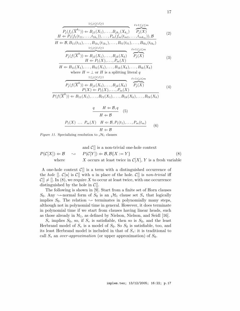
These rules can be presented in the form shown in Figure 11; we

explain them below. We write Xk

for the sequence of pairwise dis-tinct variables X1, . . . , Xk. Note that side premises can only be eitheralternating automaton clauses of the form

P (f(X1, . . . ,Xk)) ⇐ B1(X1), . . . , Bk(Xk) (1)

where B1(X1), . . . , Bk(Xk) are possibly empty ε-blocks, or universal

clauses of the form P (X), or ne-facts qB (stating that B recognizes annon-empty intersection). This is because side premises have no selected

implem.tex; 13/12/2005; 16:22; p.15

16

atom in their bodies, and because we can assume that ε-splitting doesnot apply to them. In the benchmark results presented in the sequel, weshall call “automaton” clauses all alternating automaton and universalclauses alike. These are the ones counted in the “automaton” columnof Figure 9 and other similar tables.

Resolution takes different forms, according to the form of the mainpremise. If the main premise contains a splitting symbol q (case 1. ofthe selection function), then it must unify with some ne-fact, this isrule (5) of Figure 11. Otherwise, the main premise may be in case 2.of the selection function, where there are m ≥ 1 selected non-simpleatoms P1(f1(t11, . . . , t1k1

)), . . . , Pm(fm(tm1, . . . , tmkm)). Some of them,say the first `, will unify with heads of alternating automata clauses,and the others will unify with universal clauses. This is rule (2) when` ≥ 1, and is rule (6) when ` = 0. In case 3. of the selection function,the selected literals must be all (simple) atoms in the body, and themain premise must be of the form H ⇐ P1(X), . . . , Pm(X) where H is⊥, a splitting atom, or an atom P (X) for the same variable X, becauseof our eager use of ε-splitting. In case we unify with ` ≥ 1 alternatingautomaton clauses, either H is ⊥ or a splitting atom, and we applyrule (3), or H = P (X), and we apply rule (4). If ` = 0, then we againapply rule (6).

One of the things to notice in these rules is the fact that unificationand instantiation always takes a very simple form. The role of alter-nating automaton clauses in rule (2) is to peel off one layer of functionsymbols f1, . . . , fm, and to replace variables Xi by immediate subtermstij of terms appearing in the selected atoms of the main premise. Theother rules are even simpler. A nice byproduct is that no unificationprocedure is really needed in implementing these rules.

3.2. The Standard Approximation, Converting H1 to [H1

A nice feature of H1 and [H1 is that any set of Horn clauses admitsa standard approximation, in the form of [H1 clauses. (In fact any setof clauses, Horn or not, by first approximating non-Horn clauses suchas C ∨ +A1 ∨ . . . ∨ +An by the clauses C ∨ +A1, . . . , C ∨ +An, asdone in Flotter [26].) Recall that we use the letter B to denote finitesets of atoms—clause bodies. In the sequel, BX := t denotes B witht substituted for X. Define the rewrite relation ; on Horn clause setsby:

P (C[t]) ⇐ B ;

P (C[Z]) ⇐ B, Q(Z) (Z fresh)

Q(t) ⇐ B(7)

where t is not a variable, Q is a fresh predicate symbol,

implem.tex; 13/12/2005; 16:22; p.16

17

1≤j≤`,`≥1︷︸︸︷Pj(fj(X

kj)) ⇐ Bj1(X1), . . . , Bjkj

(Xkj)

`+1≤j≤m︷︸︸︷Pj(X)

H ⇐ P1(f1(t11, . . . , t1k1)), . . . , Pm(fm(tm1, . . . , tmkm

)),B

H ⇐ B, B11(t11), . . . , B1k1(t1k1

), . . . , B`1(t`1), . . . , B`k`(t`k`

)

(2)

1≤j≤`,`≥1︷︸︸︷Pj(f(X

k)) ⇐ Bj1(X1), . . . , Bjk(Xk)

`+1≤j≤m︷︸︸︷Pj(X)

H ⇐ P1(X), . . . , Pm(X)

H ⇐ B11(X1), . . . , B`1(X1), . . . , B1k(Xk), . . . , B`k(Xk)

(3)

where H = ⊥ or H is a splitting literal q1≤j≤`,`≥1︷︸︸︷

Pj(f(Xk)) ⇐ Bj1(X1), . . . , Bjk(Xk)

`+1≤j≤m︷︸︸︷Pj(X)

P (X) ⇐ P1(X), . . . , Pm(X)

P (f(Xk)) ⇐ B11(X1), . . . , B`1(X1), . . . , B1k(Xk), . . . , B`k(Xk)

(4)

q H ⇐ B, q

H ⇐ B(5)

P1(X) . . . Pm(X) H ⇐ B, P1(t1), . . . , Pm(tm)

H ⇐ B(6)

Figure 11. Specializing resolution to [H1 clauses

and C[] is a non-trivial one-hole context

P (C[X]) ⇐ B ; P (C[Y ]) ⇐ B,BX := Y (8)

where X occurs at least twice in C[X], Y is a fresh variable

A one-hole context C[] is a term with a distinguished occurrence ofthe hole []. C[u] is C[] with u in place of the hole. C[] is non-trivial iffC[] 6= []. In (8), we requireX to occur at least twice, with one occurrencedistinguished by the hole in C[].

The following is shown in [9]. Start from a finite set of Horn clausesS0. Any ;-normal form of S0 is an [H1 clause set S∗ that logicallyimplies S0. The relation ; terminates in polynomially many steps,although not in polynomial time in general. However, it does terminatein polynomial time if we start from clauses having linear heads, suchas those already in H1, as defined by Nielson, Nielson, and Seidl [16].S∗ implies S0, so, if S∗ is satisfiable, then so is S0, and the least

Herbrand model of S∗ is a model of S0. So S0 is satisfiable, too, andits least Herbrand model is included in that of S∗: it is traditional tocall S∗ an over-approximation (or upper approximation) of S0.

implem.tex; 13/12/2005; 16:22; p.17

18

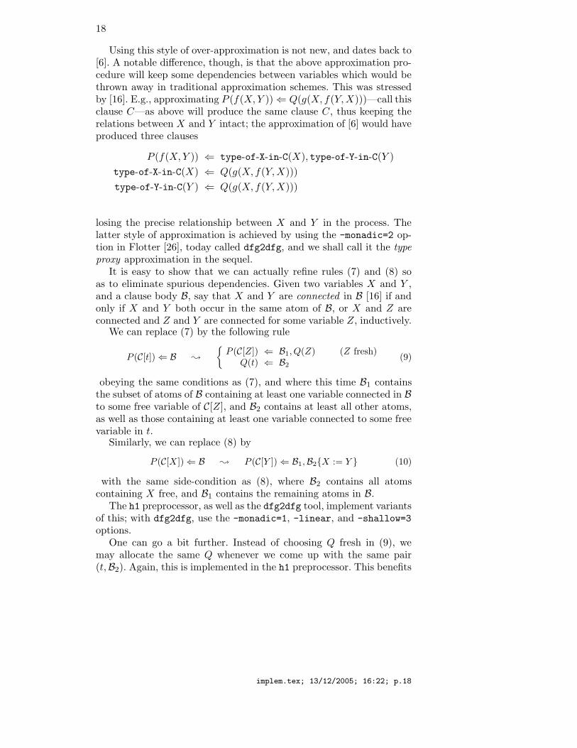
Using this style of over-approximation is not new, and dates back to[6]. A notable difference, though, is that the above approximation pro-cedure will keep some dependencies between variables which would bethrown away in traditional approximation schemes. This was stressedby [16]. E.g., approximating P (f(X,Y )) ⇐ Q(g(X, f(Y,X)))—call thisclause C—as above will produce the same clause C, thus keeping therelations between X and Y intact; the approximation of [6] would haveproduced three clauses

P (f(X,Y )) ⇐ type-of-X-in-C(X), type-of-Y-in-C(Y )

type-of-X-in-C(X) ⇐ Q(g(X, f(Y,X)))

type-of-Y-in-C(Y ) ⇐ Q(g(X, f(Y,X)))

losing the precise relationship between X and Y in the process. Thelatter style of approximation is achieved by using the -monadic=2 op-tion in Flotter [26], today called dfg2dfg, and we shall call it the type

proxy approximation in the sequel.It is easy to show that we can actually refine rules (7) and (8) so

as to eliminate spurious dependencies. Given two variables X and Y ,and a clause body B, say that X and Y are connected in B [16] if andonly if X and Y both occur in the same atom of B, or X and Z areconnected and Z and Y are connected for some variable Z, inductively.

We can replace (7) by the following rule

P (C[t]) ⇐ B ;

P (C[Z]) ⇐ B1, Q(Z) (Z fresh)

Q(t) ⇐ B2(9)

obeying the same conditions as (7), and where this time B1 containsthe subset of atoms of B containing at least one variable connected in Bto some free variable of C[Z], and B2 contains at least all other atoms,as well as those containing at least one variable connected to some freevariable in t.

Similarly, we can replace (8) by

P (C[X]) ⇐ B ; P (C[Y ]) ⇐ B1,B2X := Y (10)

with the same side-condition as (8), where B2 contains all atomscontaining X free, and B1 contains the remaining atoms in B.

The h1 preprocessor, as well as the dfg2dfg tool, implement variantsof this; with dfg2dfg, use the -monadic=1, -linear, and -shallow=3

options.One can go a bit further. Instead of choosing Q fresh in (9), we

may allocate the same Q whenever we come up with the same pair(t,B2). Again, this is implemented in the h1 preprocessor. This benefits

implem.tex; 13/12/2005; 16:22; p.18

19

subsequent proof search: if we had generated k fresh symbols for thesame pair, then any resolution inference involving Q(t) ⇐ B2 as themain premise would have to be done k times, a clear loss of time. Theabbreviation rule of Section 5 is in the same spirit.

In general, one may think that coarser approximations should lead tofaster proof search. We have seen in Section 1.3 that this was certainlytrue for 116 of the 808 TPTP examples, whose unapproximated formis not known to be satisfiable or not, but whose approximated formwas (easily) decidable. This was certainly wrong for the Parrennesexamples, which are hard, but whose original unapproximated formis reasonably easy (using SPASS with the right options). We shouldnot conclude that there is such a formal connection between precisionof an approximation and subsequent efficiency of proof search.

One may also think that coarser approximations will result in extraloss of precision. While this is true, formally, Figure 2 shows that notmuch precision is lost in general. We do not lose more in general inpassing to the type proxy approximation: all of the H1 clause sets fromthe Parrennes and TPTP examples whose type proxy approximationwas found to be unsatisfiable were indeed unsatisfiable.

4. Quickly Finding Over-approximations of the Least

Herbrand Model

Before h1 starts to saturate a given [H1 clause set using ordered resolu-tion with selection and ε-splitting, it computes an over-approximationof the least Herbrand model of the subset of definite clauses.

The first algorithm we implemented to do so was very naive. Strangelyenough, and although we tested many variants or even different ideas,the one algorithm that seems to work best is very close to this initialalgorithm. Here it is.

4.1. Pathsets

The main data structure is the pathset . A pathset is either the specialcatch-all constant Ω, or a finite map (i.e., a table) from pairs (f, i) topathsets π; the pairs (f, i) consist of a function symbol f , say of arityn, and an integer i, which must be 0 if n = 0 (i.e., f is a constant),and otherwise is such that 1 ≤ i ≤ n. We require that pathsets arenormalized: if i = 0, then (f, i) can only be mapped to Ω; moreover,any pair (f, i) is mapped to a non-empty pathset π, i.e., either Ω or anon-empty map.

Pathsets are concise representations of sets of paths through groundterms. A path is just a finite non-empty sequence of pairs (f, i) as above,

implem.tex; 13/12/2005; 16:22; p.19

20

where only the final pair has i = 0. Given a ground term t, the paths

through t are defined as follows. If t is a constant c, then (c, 0) is theonly path through t. Otherwise, say t = f(t1, . . . , tn), with n ≥ 1; thenthe paths through t are all sequences (f, i).π, where 1 ≤ i ≤ n, and πranges over the paths through ti.

In general, the semantics paths(ψ) of pathsets ψ is given as follows:paths(Ω) is the set of all ground terms, while for any ψ 6= Ω, paths(ψ) =(f, i).π|(f, i) ∈ domψ, i 6= 0, π ∈ terms(ψ(f, i)) ∪ (c, 0)|(c, 0) ∈domψ.

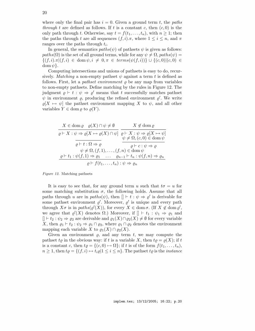
Computing intersections and unions of pathsets is easy to do, recur-sively. Matching a non-empty pathset ψ against a term t is defined asfollows. First, let a pathset environment % be any map from variablesto non-empty pathsets. Define matching by the rules in Figure 12. Thejudgment % ` t : ψ ⇒ %′ means that t successfully matches pathsetψ in environment %, producing the refined environment %′. We write%[X 7→ ψ] the pathset environment mapping X to ψ, and all othervariables Y ∈ dom % to %(Y ).

X ∈ dom % %(X) ∩ ψ 6= ∅

% ` X : ψ ⇒ %[X 7→ %(X) ∩ ψ]

X 6∈ dom %

% ` X : ψ ⇒ %[X 7→ ψ]

% ` t : Ω ⇒ %

ψ 6= Ω, (c, 0) ∈ domψ

% ` c : ψ ⇒ %ψ 6= Ω, (f, 1), . . . , (f, n) ∈ domψ

% ` t1 : ψ(f, 1) ⇒ %1 . . . %n−1 ` tn : ψ(f, n) ⇒ %n

% ` f(t1, . . . , tn) : ψ ⇒ %n

Figure 12. Matching pathsets

It is easy to see that, for any ground term u such that tσ = u forsome matching substitution σ, the following holds. Assume that allpaths through u are in paths(ψ), then [] ` t : ψ ⇒ %′ is derivable forsome pathset environment %′. Moreover, %′ is unique and every paththrough Xσ is in paths(%′(X)), for every X ∈ domσ. (If X 6∈ dom %′,we agree that %′(X) denotes Ω.) Moreover, if [] ` t1 : ψ1 ⇒ %1 and[] ` t2 : ψ2 ⇒ %2 are derivable and %1(X)∩%2(X) 6= ∅ for every variableX, then %1 ` t2 : ψ2 ⇒ %1 ∩ %2, where %1 ∩ %2 denotes the environmentmapping each variable X to %1(X) ∩ %2(X).

Given an environment %, and any term t, we may compute thepathset t% in the obvious way: if t is a variable X, then t% = %(X); if tis a constant c, then t% = (c, 0) 7→ Ω; if t is of the form f(t1, . . . , tn),n ≥ 1, then t% = (f, i) 7→ ti%|1 ≤ i ≤ n. The pathset t% is the instance

implem.tex; 13/12/2005; 16:22; p.20

21

of t by %. Clearly, if every path through Xσ is in paths(%(X)), for everyvariable X ∈ domσ, then every path through tσ is in paths(t%).

The final operation we need is chopping . In general, we require chopto be a function from pathsets to pathsets such that paths(chop(ψ)) ⊇paths(ψ), and such that the range of chop is finite. In practice, chop(ψ)replaces any sub-pathset at depth greater than some fixed bound k ∈ N

by Ω. Formally, chop = chopk, where chop0(ψ) = Ω, and if ψ 6= Ω thenchopk+1(ψ) = (f, i) 7→ chopk(ψ(f, i))|(f, i) ∈ domψ.

We then approximate least Herbrand models by pathset structures,which are by definition finite maps from predicate symbols to pathsets.Intuitively, if P (u) is in the least Herbrand model of a given set ofclauses, we wish to compute a pathset structure Ψ∞ that will map Pto a pathset ψ such that paths(ψ) contains at least all paths through u.Any pathset structure Ψ can also be seen as the set of all pairs (P, π),P ∈ domΨ, π ∈ paths(Ψ(P )); implementing unions of pathsets is thenformally defined, and again easy to implement.

A clause body B = P1(t1), . . . , Pn(tn) matches a pathset structureΨ, yielding the matcher %, if and only if

[] ` t1 : Ψ(P1) ⇒ %1 . . . %n−1 ` tn : Ψ(Pn) ⇒ %n

and %n = %. We shall write this Ψ B ⇒ %. In case no such derivationis possible, we write Ψ 6 B ⇒.

The desired over-approximation Ψ∞ can be computed as a leastfixpoint of an operator resembling the TP operator of Prolog semantics.Let S be a set of Horn clauses, and assume for the sake of readabilitythat ⊥ is just another predicate, so that ⊥% is well-defined and equalto ⊥. For any pathset structure Ψ, define

T ]S(Ψ) = Ψ ∪ chop(H%)|∃(H ⇐ B) ∈ S · Ψ B ⇒ %

The least fixpoint of T ]S is the Ψ∞ we longed for. It is computable,

by standard fixpoint iteration algorithms. E.g., let Ψ0 be the empty

pathset, then compute Ψn+1 = Ψn ∪ T ]S(Ψn) until Ψn+1 = Ψn. This

terminates because chop has finite range. Also, it is clear that Ψ∞ issound , in that: first, if ⊥ is derivable from S, then ⊥ is in the domainof Ψ∞; and second, if the ground atom P (u) is derivable from S, thenpaths(Ψ(P )) contains all paths through u.

In particular, if ⊥ is not in the domain of Ψ∞, then S is satisfiable.This very rarely happens in practical situations. The main purpose ofΨ∞ is different.

implem.tex; 13/12/2005; 16:22; p.21

22

4.2. Using Pathsets Profitably

Pathsets can then be used to do static soft typing. Typically, if resolu-tion generates a clause H ⇐ B, and Ψ∞ 6 B ⇒, then remove H ⇐ B.Call this rule naive static soft typing—naivete refers to the fact thatΨ∞ was computed rather naively.

We observe that this preserves completeness in all calculi that can beproved complete by Bachmair and Ganzinger’s forcing technique: see[22, Section 6.7]. And ordered resolution with selection, and all forms ofsplitting we use, are complete by Bachmair and Ganzinger’s technique.

In the presence of ε-splitting, this involves a subtle point: since thelanguage of predicates is augmented whenever a fresh ne-fact qB isproduced, we need to recompute Ψ∞. Remember that such ne-facts aregenerated when ε-splitting clauses of the form A⇐ B, B(X), where Xis not free in A, B. To recompute Ψ∞, we need to adjust Ψ∞ against thefresh defining clause qB ⇐ B(X) in particular. It is easy to see thatdoing so merely amounts to adding qB 7→ Ω to Ψ∞ whenever theintersection

⋂P∈B Ψ∞(P ) is non-empty. When

⋂P∈B Ψ∞(P ) is empty,

then Ψ∞ 6 B(X) ⇒, so Ψ∞ 6 B, B(X), and we remove A⇐ B, B(X)from the current clause set instead.

Call ne-fact pruning the special case of naive static soft typing thatconsists in removing clauses A ⇐ B, B(X) such that

⋂P∈B Ψ∞(P ) is

empty, and generating qB only when⋂

P∈B Ψ∞(P ) is not empty. Thene-fact pruning rule initially seemed very effective. We have observed,during early stages of the development of h1, that ne-fact pruningaccounted for a great majority of the cases where naive static softtyping applied. In old versions, naive static soft typing accounted formassive reductions in the search space. In the current version of h1,other optimizations muddy the picture.

We have therefore tried to evaluate the impact of naive static softtyping by comparing the results of Section 1.1 with those obtained onthe same clause sets, this time with naive static soft typing deactivated.Technically, it suffices to call h1 with the -path-refine 0 option,which implements chop as chop0, hence computes path structures thatmap each predicate to Ω. We estimate the overhead of computing withpathsets restricted to Ω (instead of really excising the pathset code) tobe negligible.

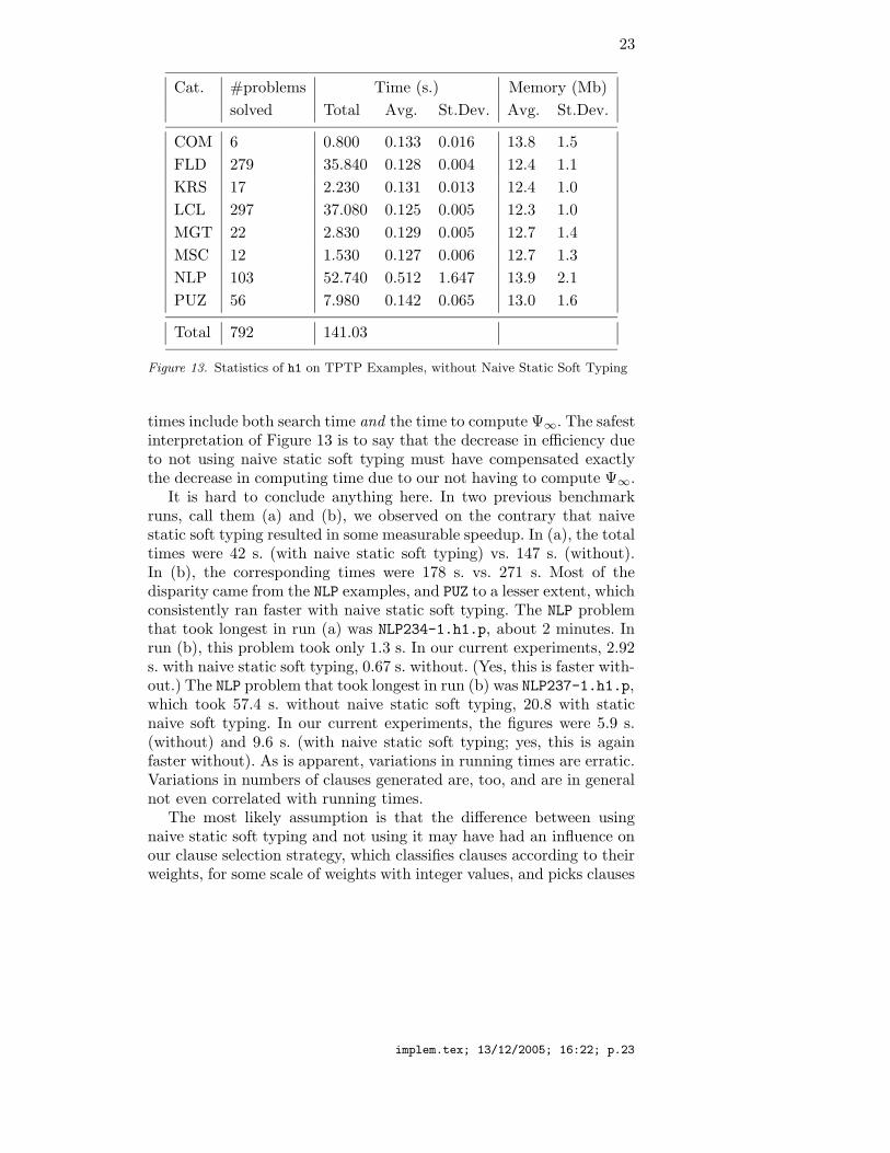
The results are shown in Figure 13 for the TPTP examples. Thenumber of problems solved is the same. (Previous experiments haveexhibited a variation of ±1 problem solved.) And the total running timewas identical, too. However, observe that total running time is a poorindicator of performance, not only because, as we have already seen,we should expect variations of about ±15%, but also because running

implem.tex; 13/12/2005; 16:22; p.22

23



COM 6 0.800 0.133 0.016 13.8 1.5

FLD 279 35.840 0.128 0.004 12.4 1.1

KRS 17 2.230 0.131 0.013 12.4 1.0

LCL 297 37.080 0.125 0.005 12.3 1.0

MGT 22 2.830 0.129 0.005 12.7 1.4

MSC 12 1.530 0.127 0.006 12.7 1.3

NLP 103 52.740 0.512 1.647 13.9 2.1

PUZ 56 7.980 0.142 0.065 13.0 1.6

Total 792 141.03

Figure 13. Statistics of h1 on TPTP Examples, without Naive Static Soft Typing

times include both search time and the time to compute Ψ∞. The safestinterpretation of Figure 13 is to say that the decrease in efficiency dueto not using naive static soft typing must have compensated exactlythe decrease in computing time due to our not having to compute Ψ∞.

It is hard to conclude anything here. In two previous benchmarkruns, call them (a) and (b), we observed on the contrary that naivestatic soft typing resulted in some measurable speedup. In (a), the totaltimes were 42 s. (with naive static soft typing) vs. 147 s. (without).In (b), the corresponding times were 178 s. vs. 271 s. Most of thedisparity came from the NLP examples, and PUZ to a lesser extent, whichconsistently ran faster with naive static soft typing. The NLP problemthat took longest in run (a) was NLP234-1.h1.p, about 2 minutes. Inrun (b), this problem took only 1.3 s. In our current experiments, 2.92s. with naive static soft typing, 0.67 s. without. (Yes, this is faster with-out.) The NLP problem that took longest in run (b) was NLP237-1.h1.p,which took 57.4 s. without naive static soft typing, 20.8 with staticnaive soft typing. In our current experiments, the figures were 5.9 s.(without) and 9.6 s. (with naive static soft typing; yes, this is againfaster without). As is apparent, variations in running times are erratic.Variations in numbers of clauses generated are, too, and are in generalnot even correlated with running times.

The most likely assumption is that the difference between usingnaive static soft typing and not using it may have had an influence onour clause selection strategy, which classifies clauses according to theirweights, for some scale of weights with integer values, and picks clauses

implem.tex; 13/12/2005; 16:22; p.23

24

non-deterministically amongst those of equal weights. (We briefly de-scribe our weight system in Section 6.) To be precise, clauses of equalweight are stored in a HimML map [8]. Depending on memory layout,and the history of memory allocation, the order in which elementsof a HimML map are stored can vary wildly. Any change in memoryallocation may result in a different clause selection strategy. This musthave obscured any effect that static soft typing may have had by itself.

On the other hand, most of the TPTP examples are easy. On aver-age, they are solved within 0.178 s., from which, remember, we mustdiscount 0.12 of startup time. To really evaluate naive static soft typing,we should turn to more complex examples, and possibly ones on whichclause selection has little effect. The Parrennes examples fit the bill.

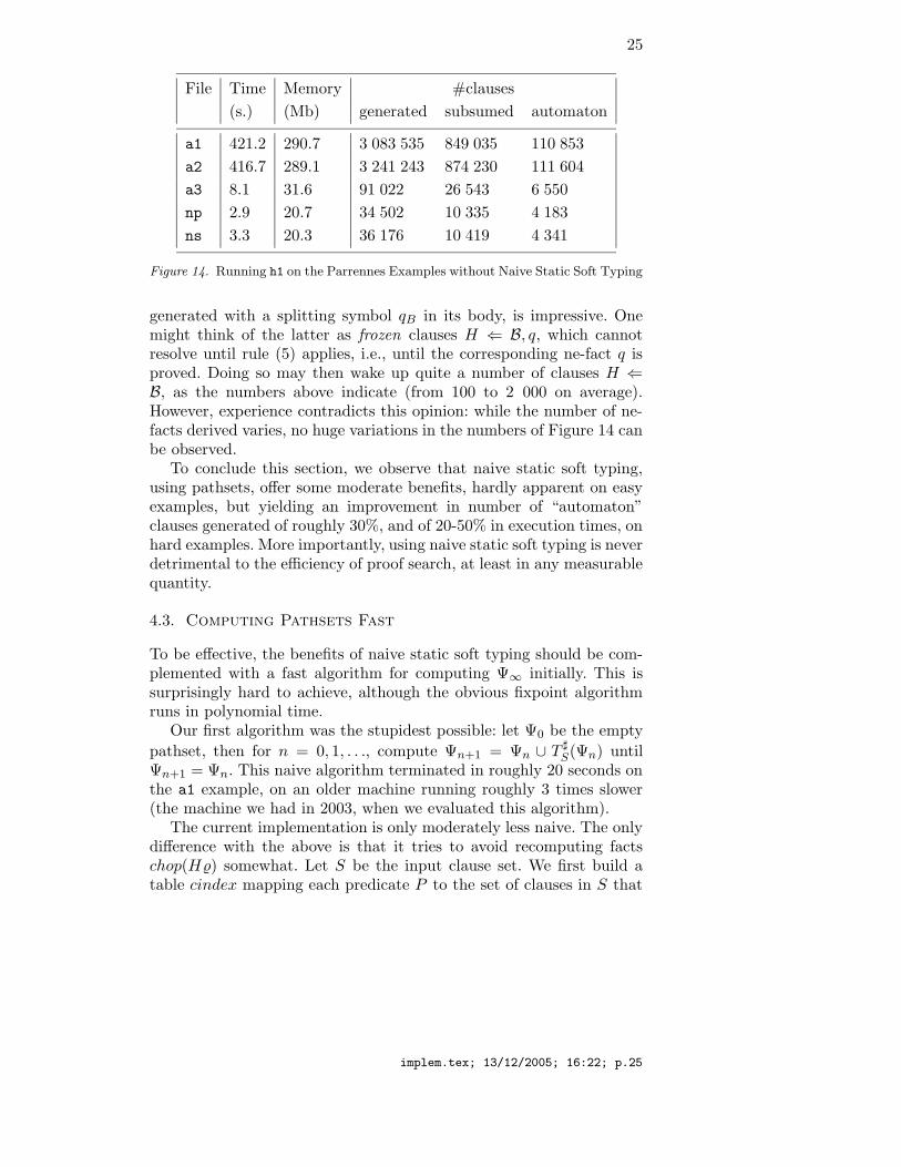
Look at Figure 14. Computation times are slower by 0 to 50%without naive static soft typing: 18% for a1, 52% for a2, 6.5% fora3, 0% for np, 50% for ns. However, we have noticed several timesthat computation times were a poor indicator of performance. Naivestatic soft typing does not make much difference in number of clausesgenerated: only 6% more for the hard examples a1 and a2, 10% morefor a3, around 20% more for np and 40% more for ns. (Similarly fornumber of clauses subsumed on the hard examples; figures are probablyless significant on easy examples. In fact, the percentages indicated wereconsistently the same, up to 1%, on several experiments, except on ns

where we usually only got 20% more clauses.) The difference is clearerin terms of “automaton” clauses. Remember that “automaton” clausesare those where no literal is selected, and are those that participate inresolution as side premises. Remember also that, although resolutiononly uses one main premise, it uses as many side premises as there areselected literals in the main premise. So a small increase in “automaton”clauses may result in dramatic loss of performance. Here, naive staticsoft typing resulted in generating about 30% less “automaton” clauses(a1, a2), resp. 20% less (a3), resp. 40% less (np, ns). (All percentagesgiven in this paragraph were the same in previous experiments again,except for np and ns, where the percentage used to be in the regionaround 20%.)

One figure that does not appear in the above tables is the number ofne-facts generated. With naive static soft typing, they are respectively658 (1 456 696 clauses split), 718 (1 550 665 clauses split), 173 (36 052clauses split), 148 (11 713 clauses split), 160 (13 229 clauses split).Without, these numbers become 663 (1 575 574), 715 (1 661 714), 173(40 834), 151 (16 644), and 162 (18 185). Again, these figures wereremarkably impervious to benchmark reruns. We conclude that ne-factpruning has no measurable impact. Note however that, while only veryfew ne-facts are generated, the number of clauses split, hence of clauses

implem.tex; 13/12/2005; 16:22; p.24

25



a1 421.2 290.7 3 083 535 849 035 110 853

a2 416.7 289.1 3 241 243 874 230 111 604

a3 8.1 31.6 91 022 26 543 6 550

np 2.9 20.7 34 502 10 335 4 183

ns 3.3 20.3 36 176 10 419 4 341

Figure 14. Running h1 on the Parrennes Examples without Naive Static Soft Typing

generated with a splitting symbol qB in its body, is impressive. Onemight think of the latter as frozen clauses H ⇐ B, q, which cannotresolve until rule (5) applies, i.e., until the corresponding ne-fact q isproved. Doing so may then wake up quite a number of clauses H ⇐B, as the numbers above indicate (from 100 to 2 000 on average).However, experience contradicts this opinion: while the number of ne-facts derived varies, no huge variations in the numbers of Figure 14 canbe observed.

To conclude this section, we observe that naive static soft typing,using pathsets, offer some moderate benefits, hardly apparent on easyexamples, but yielding an improvement in number of “automaton”clauses generated of roughly 30%, and of 20-50% in execution times, onhard examples. More importantly, using naive static soft typing is neverdetrimental to the efficiency of proof search, at least in any measurablequantity.

4.3. Computing Pathsets Fast

To be effective, the benefits of naive static soft typing should be com-plemented with a fast algorithm for computing Ψ∞ initially. This issurprisingly hard to achieve, although the obvious fixpoint algorithmruns in polynomial time.

Our first algorithm was the stupidest possible: let Ψ0 be the empty

pathset, then for n = 0, 1, . . ., compute Ψn+1 = Ψn ∪ T ]S(Ψn) until

Ψn+1 = Ψn. This naive algorithm terminated in roughly 20 seconds onthe a1 example, on an older machine running roughly 3 times slower(the machine we had in 2003, when we evaluated this algorithm).

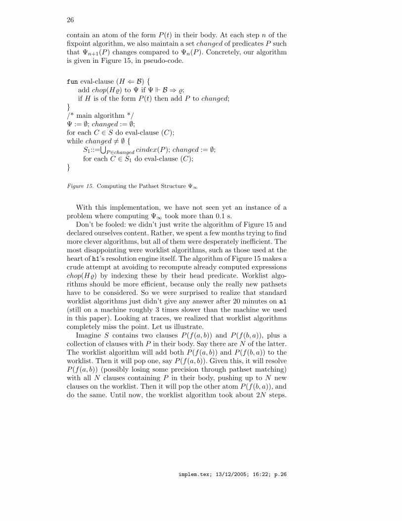
The current implementation is only moderately less naive. The onlydifference with the above is that it tries to avoid recomputing factschop(H%) somewhat. Let S be the input clause set. We first build atable cindex mapping each predicate P to the set of clauses in S that

implem.tex; 13/12/2005; 16:22; p.25

26

contain an atom of the form P (t) in their body. At each step n of thefixpoint algorithm, we also maintain a set changed of predicates P suchthat Ψn+1(P ) changes compared to Ψn(P ). Concretely, our algorithmis given in Figure 15, in pseudo-code.

fun eval-clause (H ⇐ B) add chop(H%) to Ψ if Ψ B ⇒ %;if H is of the form P (t) then add P to changed;

/* main algorithm */Ψ := ∅; changed := ∅;for each C ∈ S do eval-clause (C);while changed 6= ∅

S1::=⋃

P∈changed cindex(P ); changed := ∅;for each C ∈ S1 do eval-clause (C);

Figure 15. Computing the Pathset Structure Ψ∞

With this implementation, we have not seen yet an instance of aproblem where computing Ψ∞ took more than 0.1 s.

Don’t be fooled: we didn’t just write the algorithm of Figure 15 anddeclared ourselves content. Rather, we spent a few months trying to findmore clever algorithms, but all of them were desperately inefficient. Themost disappointing were worklist algorithms, such as those used at theheart of h1’s resolution engine itself. The algorithm of Figure 15 makes acrude attempt at avoiding to recompute already computed expressionschop(H%) by indexing these by their head predicate. Worklist algo-rithms should be more efficient, because only the really new pathsetshave to be considered. So we were surprised to realize that standardworklist algorithms just didn’t give any answer after 20 minutes on a1

(still on a machine roughly 3 times slower than the machine we usedin this paper). Looking at traces, we realized that worklist algorithmscompletely miss the point. Let us illustrate.

Imagine S contains two clauses P (f(a, b)) and P (f(b, a)), plus acollection of clauses with P in their body. Say there are N of the latter.The worklist algorithm will add both P (f(a, b)) and P (f(b, a)) to theworklist. Then it will pop one, say P (f(a, b)). Given this, it will resolveP (f(a, b)) (possibly losing some precision through pathset matching)with all N clauses containing P in their body, pushing up to N newclauses on the worklist. Then it will pop the other atom P (f(b, a)), anddo the same. Until now, the worklist algorithm took about 2N steps.

implem.tex; 13/12/2005; 16:22; p.26

27

In general, if there were m unit clauses, not just 2, with head P , theworklist algorithm would take about mN steps until now.

The algorithm of Figure 15, instead, takes P (f(a, b)) and P (f(b, a)),adds them both to Ψ. This yields a pathset structure mapping P to thefour paths (f, 1).(a, 0).Ω, (f, 2).(b, 0).Ω, (f, 1).(b, 0).Ω, and (f, 2).(a, 0).Ω.(In particular, we lose precision: we cannot rule out matching P (f(a, a))or P (f(b, b)) against Ψ.) Next, there are N clauses with P in theirbodies. Examining them takes N units of time, for a total of N + 2—N +m in the general case where there are m, not just 2, initial clausesto consider.

We have therefore replaced mN operations by m + N . This holdsinitially, i.e., at step 0 of the fixpoint algorithm, but in fact at everystep of this algorithm. At later steps, the number m of facts to considerin worklist algorithms usually grows as a polynomial in the numberof function symbols in the signature (whose degree depends on thelevel at which terms are chopped), while m is bounded by the numberof clauses nC in the algorithm of Figure 15. Precisely, let nf be thenumber of function symbols and np the number of predicate symbols, athe maximal arity of function symbols, and k the level at which termsare chopped. Then m can be as large as np(1 + nf (1 + nf (. . . (1 +

nf )a . . .)a) ≤ np(1 + nf )akin the worklist algorithm, while m ≤ np in

the algorithm of Figure 15. We have therefore reduced the complexity

of finding Ψ∞ from roughly np(1 + nf )akN to nC + N at each step.

In the a1 example, nf is large but only 11 functions are not constants.The number of possible pathsets is however at least np11kN . Withnp = 730, N ≈ nC = 1 161, and k = 3, the worklist algorithm mayhave to consider about 109 pathsets at each step while the algorithmof Figure 15 only has to consider at most 2 322. . . quite a reduction.

4.4. Less Naive Static Soft Typing

Instead of using ad hoc pathset structures, an easy way to compute amore precise over-approximation is to use type proxies. In other words,compute the type proxy approximation Sproxy of the given [H1 clauseset S, then run h1 itself a first time on Sproxy. Hopefully, this shouldrun faster than on S directly. If Sproxy is satisfiable, then S is, too, andwe are done. Otherwise, h1 will output an alternating automaton (i.e.,sets of clauses of the form (1), plus universal clauses) that describes afinite model M of the subset of definite clauses in Sproxy. (To get themodel explicitly, determinize and complete the automaton; the statesof the resulting automaton A form the domain of the model, and thevalue of f on values q1, . . . , qn is the unique state q such that there isa transition q(f(X1, . . . ,Xn)) ⇐ q1(X1), . . . , qn(Xn) in A. More details

implem.tex; 13/12/2005; 16:22; p.27

28

in [10].) Using M, a collection of regular tree languages, as an over-approximation of the least Herbrand model of S if any, is closer to theoriginal spirit of static soft typing for resolution.

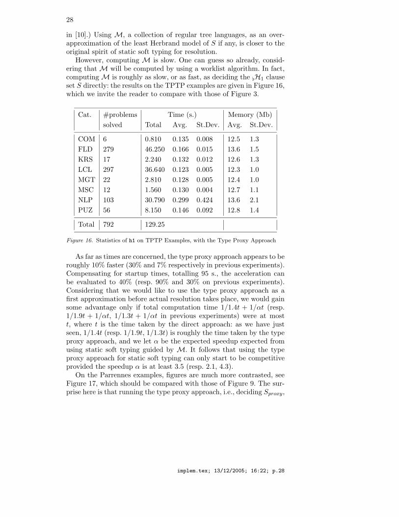
However, computing M is slow. One can guess so already, consid-ering that M will be computed by using a worklist algorithm. In fact,computing M is roughly as slow, or as fast, as deciding the [H1 clauseset S directly: the results on the TPTP examples are given in Figure 16,which we invite the reader to compare with those of Figure 3.



COM 6 0.810 0.135 0.008 12.5 1.3

FLD 279 46.250 0.166 0.015 13.6 1.5

KRS 17 2.240 0.132 0.012 12.6 1.3

LCL 297 36.640 0.123 0.005 12.3 1.0

MGT 22 2.810 0.128 0.005 12.4 1.0

MSC 12 1.560 0.130 0.004 12.7 1.1

NLP 103 30.790 0.299 0.424 13.6 2.1

PUZ 56 8.150 0.146 0.092 12.8 1.4

Total 792 129.25

Figure 16. Statistics of h1 on TPTP Examples, with the Type Proxy Approach

As far as times are concerned, the type proxy approach appears to beroughly 10% faster (30% and 7% respectively in previous experiments).Compensating for startup times, totalling 95 s., the acceleration canbe evaluated to 40% (resp. 90% and 30% on previous experiments).Considering that we would like to use the type proxy approach as afirst approximation before actual resolution takes place, we would gainsome advantage only if total computation time 1/1.4t + 1/αt (resp.1/1.9t + 1/αt, 1/1.3t + 1/αt in previous experiments) were at mostt, where t is the time taken by the direct approach: as we have justseen, 1/1.4t (resp. 1/1.9t, 1/1.3t) is roughly the time taken by the typeproxy approach, and we let α be the expected speedup expected fromusing static soft typing guided by M. It follows that using the typeproxy approach for static soft typing can only start to be competitiveprovided the speedup α is at least 3.5 (resp. 2.1, 4.3).

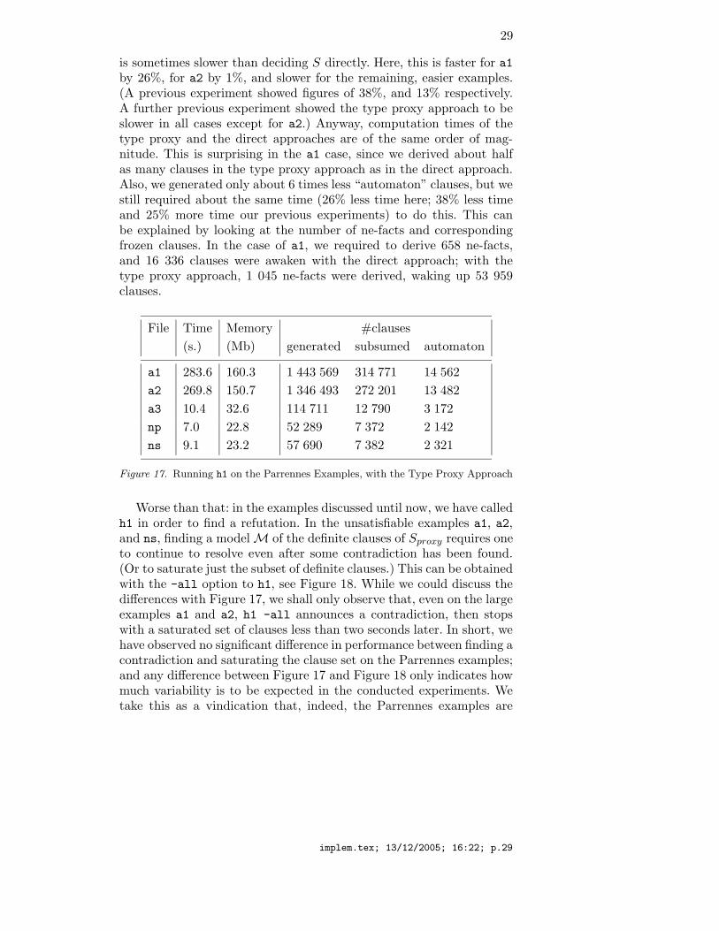
On the Parrennes examples, figures are much more contrasted, seeFigure 17, which should be compared with those of Figure 9. The sur-prise here is that running the type proxy approach, i.e., deciding Sproxy,

implem.tex; 13/12/2005; 16:22; p.28

29

is sometimes slower than deciding S directly. Here, this is faster for a1by 26%, for a2 by 1%, and slower for the remaining, easier examples.(A previous experiment showed figures of 38%, and 13% respectively.A further previous experiment showed the type proxy approach to beslower in all cases except for a2.) Anyway, computation times of thetype proxy and the direct approaches are of the same order of mag-nitude. This is surprising in the a1 case, since we derived about halfas many clauses in the type proxy approach as in the direct approach.Also, we generated only about 6 times less “automaton” clauses, but westill required about the same time (26% less time here; 38% less timeand 25% more time our previous experiments) to do this. This canbe explained by looking at the number of ne-facts and correspondingfrozen clauses. In the case of a1, we required to derive 658 ne-facts,and 16 336 clauses were awaken with the direct approach; with thetype proxy approach, 1 045 ne-facts were derived, waking up 53 959clauses.



a1 283.6 160.3 1 443 569 314 771 14 562

a2 269.8 150.7 1 346 493 272 201 13 482

a3 10.4 32.6 114 711 12 790 3 172

np 7.0 22.8 52 289 7 372 2 142

ns 9.1 23.2 57 690 7 382 2 321

Figure 17. Running h1 on the Parrennes Examples, with the Type Proxy Approach

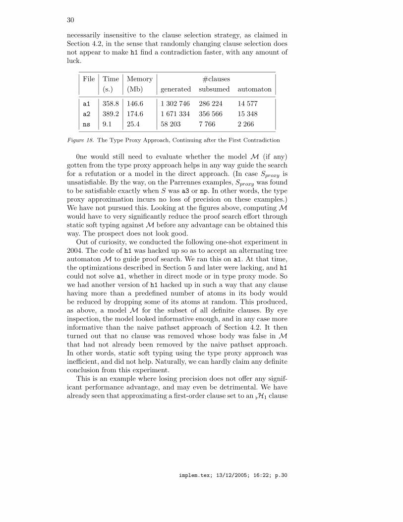
Worse than that: in the examples discussed until now, we have calledh1 in order to find a refutation. In the unsatisfiable examples a1, a2,and ns, finding a model M of the definite clauses of Sproxy requires oneto continue to resolve even after some contradiction has been found.(Or to saturate just the subset of definite clauses.) This can be obtainedwith the -all option to h1, see Figure 18. While we could discuss thedifferences with Figure 17, we shall only observe that, even on the largeexamples a1 and a2, h1 -all announces a contradiction, then stopswith a saturated set of clauses less than two seconds later. In short, wehave observed no significant difference in performance between finding acontradiction and saturating the clause set on the Parrennes examples;and any difference between Figure 17 and Figure 18 only indicates howmuch variability is to be expected in the conducted experiments. Wetake this as a vindication that, indeed, the Parrennes examples are

implem.tex; 13/12/2005; 16:22; p.29

30

necessarily insensitive to the clause selection strategy, as claimed inSection 4.2, in the sense that randomly changing clause selection doesnot appear to make h1 find a contradiction faster, with any amount ofluck.



a1 358.8 146.6 1 302 746 286 224 14 577

a2 389.2 174.6 1 671 334 356 566 15 348

ns 9.1 25.4 58 203 7 766 2 266

Figure 18. The Type Proxy Approach, Continuing after the First Contradiction

0ne would still need to evaluate whether the model M (if any)gotten from the type proxy approach helps in any way guide the searchfor a refutation or a model in the direct approach. (In case Sproxy isunsatisfiable. By the way, on the Parrennes examples, Sproxy was foundto be satisfiable exactly when S was a3 or np. In other words, the typeproxy approximation incurs no loss of precision on these examples.)We have not pursued this. Looking at the figures above, computing Mwould have to very significantly reduce the proof search effort throughstatic soft typing against M before any advantage can be obtained thisway. The prospect does not look good.

Out of curiosity, we conducted the following one-shot experiment in2004. The code of h1 was hacked up so as to accept an alternating treeautomaton M to guide proof search. We ran this on a1. At that time,the optimizations described in Section 5 and later were lacking, and h1

could not solve a1, whether in direct mode or in type proxy mode. Sowe had another version of h1 hacked up in such a way that any clausehaving more than a predefined number of atoms in its body wouldbe reduced by dropping some of its atoms at random. This produced,as above, a model M for the subset of all definite clauses. By eyeinspection, the model looked informative enough, and in any case moreinformative than the naive pathset approach of Section 4.2. It thenturned out that no clause was removed whose body was false in Mthat had not already been removed by the naive pathset approach.In other words, static soft typing using the type proxy approach wasinefficient, and did not help. Naturally, we can hardly claim any definiteconclusion from this experiment.

This is an example where losing precision does not offer any signif-icant performance advantage, and may even be detrimental. We havealready seen that approximating a first-order clause set to an [H1 clause

implem.tex; 13/12/2005; 16:22; p.30

31

set may result in more difficult problems, and should therefore not betoo surprised.

Instead of computing full automata to guide search, one may returnto the pathset approach, and improve it only slightly. Instead of com-puting sets of paths, compute sets of trees. This would avoir the lossof precision mentioned above: when we add P (f(a, b)) and P (f(b, a))to the current pathset Ψ, we in fact add the four paths (f, 1).(a, 0).Ω,(f, 2).(b, 0).Ω, (f, 1).(b, 0).Ω, and (f, 2).(a, 0).Ω. In particular, there isno way to tell that we didn’t want to add P (f(a, a)) or P (f(b, b)).

A cure is too replace pathsets by a suitable representation of setsof ground terms, of depth at most k, on an extended signature with afresh constant Ω denoting any ground term. We let the reader figure outfor herself how to adapt the constructions above. The basic construc-tion, replacing pathsets, would be the treeset : either Ω, or a map fromfunction symbols f , of arity n, to n-tuples of treesets. We tried this in2003, and thought at that time that the only way to implement thecorresponding fixpoint computation was by using a worklist algorithm.As we saw earlier, this is doomed to failure.

It would therefore, at least in principle, be interesting to implementthe naive fixpoint algorithm of Figure 15 on treesets rather than path-sets. Although we didn’t conduct any experiment meant to evaluatethe treeset approach, we convinced ourselves that this would probablynot be worth the trouble. The Parrennes examples are based on theidea [11] that points-to analysis can profitably be described by clauses.In particular, value(c(s, t)) means that the value stored at addresss is t (possibly). The csur analyzer of [11] generates a good deal ofaddresses, which are denoted by constants (whence the large numberof constants in the Parrennes examples), and addresses may point topointer values containing further addresses. Even if we consider onlyconstants for values of s, t, the treeset approach will necessarily derivea collection of facts value(c(a1, a2)), where a1 and a2 denote addressessuch that a1 points to a2. In other words, the treeset approach wouldnecessarily build a graph on around 350 nodes (remember there are349 constants in the examples a1, a2, a3). Worse, some clauses com-pute operations such as transitive closures, e.g., value(c(X,Z)) ⇐value(c(X,Y )), value(c(Y,Z)). (They shouldn’t, considering the se-mantics of pointers. But remember these examples came from an earlybuggy implementation of csur.) In effect, the treeset approach wouldcompute the transitive closure of a 350-vertex graph. This is pro-hibitive. In comparison, the pathset approach just computes over-app-roximations of the domain and codomain of the value(c( , )) relation.We have therefore also relinquished the treeset approach.

To sum up: naivete matters.

implem.tex; 13/12/2005; 16:22; p.31

32

5. Abbreviating Deep Atoms On-the-Fly

The ε-splitting rule is a special case of Riazanov and Voronkov’s split-ting with naming rule [18]. In turn, this rule can be generalized in thefollowing way. Given any clause

H ⇐ B,B′

where we have split the body into two disjoint conjunctions of atomsB and B′, and where the free variables of B are X1, . . . , Xm, create afresh predicate symbol TB and a fresh function symbol abbrvB of aritym, and replace the above clause by the two clauses

H ⇐ TB(abbrvB(X1, . . . ,Xm)),B′

TB(abbrvB(X1, . . . ,Xm)) ⇐ B

As for ε-splitting, and following the splitting with naming philosophy,we reuse the same predicate TB and the same function symbol abbrvBwhen we encounter the same conjunction B. It is even profitable torename variables in B so as to maximize the chances to reuse the samesymbols.

We call this rule the abbreviation rule.This rule is sound. Using Bachmair and Ganzinger’s general redun-

dancy elimination criterion, this rule is complete provided the twogenerated clauses are smaller than the premise H ⇐ B,B′, in a so-called admissible clause ordering [2]. Given our ordering on atoms,an admissible clause ordering is given by, first, comparing literals by±A ±′B if and only if A B, or ± is −, ±′ is +, and A B;second, by considering clauses as multisets of literals, compared by themultiset extension mul of .

One way to achieve completeness is to extend the ordering onatoms so that P (t) TB(t′) qB for each predicate symbol alreadypresent in the original clause set, for each ne-fact qB , and for everysymbol TB. Then completeness obtains if B contains at least one atomnot headed by a T or qB symbol, and H,B′ contains at least an atomnot headed by a T or qB symbol.

The most classical use of such rules is when B is a non-empty con-junction of atoms that has no free variable in common with the restH ⇐ B′ of the clause H ⇐ B,B′. This allows one to simulate splittingin the general case [18]. This was known in the field of logic programtransformation as the rule of definition introduction [17]. The latterwas notably used to obtain decidability results for inductive definitionsover language expressions, and quasi-cs logic programs [14].

The particular case of the abbreviation rule that we will be interestedin is the case where B is reduced to a single deep atom P (t). We say

implem.tex; 13/12/2005; 16:22; p.32

33

that P (t) is deep if and only if it is not shallow; P (t) is shallow ifand only if t is a variable of the application f(Y1, . . . , Yn) of a functionsymbol f to variables Y1, . . . , Yn, not necessarily distinct.

It is probably not clear what can be gained from such a rule. Weaddress this in a jiffy. Meanwhile, let us formalize it.

First, we need to find a canonical term t for each term t, so thatif t and t′ are renamed versions of each other, then t = t′. This canbe obtained as follows. Fix a countable enumeration of variables X0

1 ,. . . , X0

m, . . . , once and for all. Standardize the set of free variablesof each term t by enumerating the free variables of t from left to rightwithout duplication, say X1, . . . , Xm; e.g., enumerate the free variablesof f(X, g(X, f(Y,X), Y, Z,X)) as X, Y , Z. Then replace X1, . . . , Xm

by X01 , . . . , X0

m, that is, define t as tX1 := X01 , . . . ,Xm := X0

m.Let P be the set of predicate symbols and F the set of function

symbols of the original clause set. Let Q be the set of splitting symbolsqB . For any atom P (t) where P ∈ P and t is built from function symbolstaken from F , create a predicate symbol TP (bt) outside P ∪ Q, and a

function symbol abbrvP (bt) outside F . We assume that the functions

P (t) 7→ TP (bt) and P (t) 7→ abbrvP (bt) are one-to-one.

DEFINITION 2. The abbreviation of deep atoms rule is the abbrevi-ation rule restricted to the case where B is a single deep atom P (t).Concretely, this is the rule that replaces any clause

H ⇐ P (t),B

where P (t) is deep, P ∈ P, all function symbols of t are in F , and thereis at least one atom of the form Q(u) with Q ∈ P in H ⇐ B, by thetwo clauses

H ⇐ TP (bt)(abbrvP (bt)(X1, . . . ,Xm)),B

TP (bt)(abbrvP (bt)(X1, . . . ,Xm)) ⇐ P (t)

where X1, . . . , Xm are the free variables of t from left to right, enu-merated without duplication.

This is sound, and complete by Bachmair and Ganzinger’s generalredundancy elimination criterion, provided we take an ordering suchthat P (t) TQ(bu)(t

′) qB for every P ∈ P, as discussed above.To illustrate the speedups that can be achieved with this rule, run h1

with the -no-deep-abbrv option, which disables it, on the Parrennesexamples.

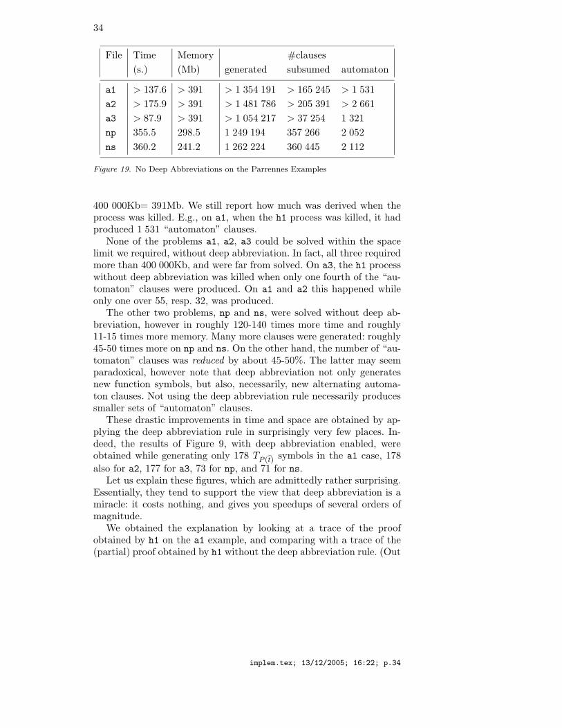
This is summed up in Figure 19. The > x entries mean that the h1

process had to be killed because it exceeded the allotted space limit of

implem.tex; 13/12/2005; 16:22; p.33

34



a1 > 137.6 > 391 > 1 354 191 > 165 245 > 1 531

a2 > 175.9 > 391 > 1 481 786 > 205 391 > 2 661

a3 > 87.9 > 391 > 1 054 217 > 37 254 1 321

np 355.5 298.5 1 249 194 357 266 2 052

ns 360.2 241.2 1 262 224 360 445 2 112

Figure 19. No Deep Abbreviations on the Parrennes Examples

400 000Kb= 391Mb. We still report how much was derived when theprocess was killed. E.g., on a1, when the h1 process was killed, it hadproduced 1 531 “automaton” clauses.

None of the problems a1, a2, a3 could be solved within the spacelimit we required, without deep abbreviation. In fact, all three requiredmore than 400 000Kb, and were far from solved. On a3, the h1 processwithout deep abbreviation was killed when only one fourth of the “au-tomaton” clauses were produced. On a1 and a2 this happened whileonly one over 55, resp. 32, was produced.

The other two problems, np and ns, were solved without deep ab-breviation, however in roughly 120-140 times more time and roughly11-15 times more memory. Many more clauses were generated: roughly45-50 times more on np and ns. On the other hand, the number of “au-tomaton” clauses was reduced by about 45-50%. The latter may seemparadoxical, however note that deep abbreviation not only generatesnew function symbols, but also, necessarily, new alternating automa-ton clauses. Not using the deep abbreviation rule necessarily producessmaller sets of “automaton” clauses.

These drastic improvements in time and space are obtained by ap-plying the deep abbreviation rule in surprisingly very few places. In-deed, the results of Figure 9, with deep abbreviation enabled, wereobtained while generating only 178 TP (bt) symbols in the a1 case, 178

also for a2, 177 for a3, 73 for np, and 71 for ns.Let us explain these figures, which are admittedly rather surprising.

Essentially, they tend to support the view that deep abbreviation is amiracle: it costs nothing, and gives you speedups of several orders ofmagnitude.

We obtained the explanation by looking at a trace of the proofobtained by h1 on the a1 example, and comparing with a trace of the(partial) proof obtained by h1 without the deep abbreviation rule. (Out

implem.tex; 13/12/2005; 16:22; p.34

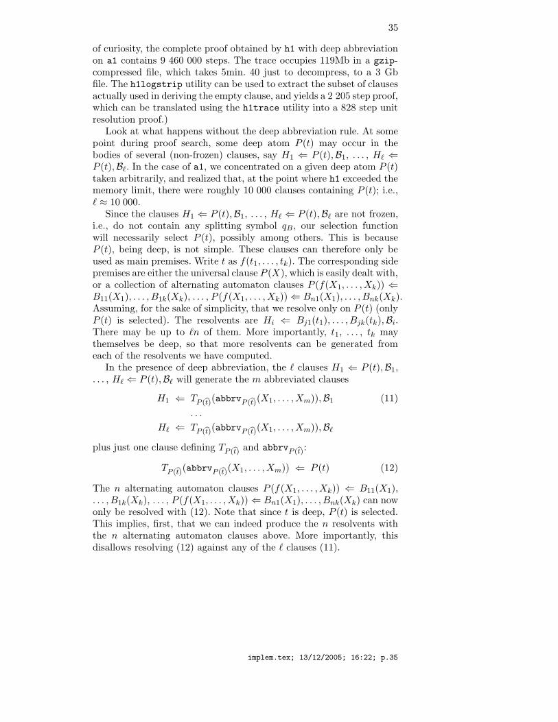
35

of curiosity, the complete proof obtained by h1 with deep abbreviationon a1 contains 9 460 000 steps. The trace occupies 119Mb in a gzip-compressed file, which takes 5min. 40 just to decompress, to a 3 Gbfile. The h1logstrip utility can be used to extract the subset of clausesactually used in deriving the empty clause, and yields a 2 205 step proof,which can be translated using the h1trace utility into a 828 step unitresolution proof.)

Look at what happens without the deep abbreviation rule. At somepoint during proof search, some deep atom P (t) may occur in thebodies of several (non-frozen) clauses, say H1 ⇐ P (t),B1, . . . , H` ⇐P (t),B`. In the case of a1, we concentrated on a given deep atom P (t)taken arbitrarily, and realized that, at the point where h1 exceeded thememory limit, there were roughly 10 000 clauses containing P (t); i.e.,` ≈ 10 000.

Since the clauses H1 ⇐ P (t),B1, . . . , H` ⇐ P (t),B` are not frozen,i.e., do not contain any splitting symbol qB, our selection functionwill necessarily select P (t), possibly among others. This is becauseP (t), being deep, is not simple. These clauses can therefore only beused as main premises. Write t as f(t1, . . . , tk). The corresponding sidepremises are either the universal clause P (X), which is easily dealt with,or a collection of alternating automaton clauses P (f(X1, . . . ,Xk)) ⇐B11(X1), . . . , B1k(Xk), . . . , P (f(X1, . . . ,Xk)) ⇐ Bn1(X1), . . . , Bnk(Xk).Assuming, for the sake of simplicity, that we resolve only on P (t) (onlyP (t) is selected). The resolvents are Hi ⇐ Bj1(t1), . . . , Bjk(tk),Bi.There may be up to `n of them. More importantly, t1, . . . , tk maythemselves be deep, so that more resolvents can be generated fromeach of the resolvents we have computed.

In the presence of deep abbreviation, the ` clauses H1 ⇐ P (t),B1,. . . , H` ⇐ P (t),B` will generate the m abbreviated clauses

H1 ⇐ TP (bt)(abbrvP (bt)(X1, . . . ,Xm)),B1 (11)

. . .

H` ⇐ TP (bt)(abbrvP (bt)(X1, . . . ,Xm)),B`

plus just one clause defining TP (bt) and abbrvP (bt):

TP (bt)(abbrvP (bt)(X1, . . . ,Xm)) ⇐ P (t) (12)

The n alternating automaton clauses P (f(X1, . . . ,Xk)) ⇐ B11(X1),. . . , B1k(Xk), . . . , P (f(X1, . . . ,Xk)) ⇐ Bn1(X1), . . . , Bnk(Xk) can nowonly be resolved with (12). Note that since t is deep, P (t) is selected.This implies, first, that we can indeed produce the n resolvents withthe n alternating automaton clauses above. More importantly, thisdisallows resolving (12) against any of the ` clauses (11).

implem.tex; 13/12/2005; 16:22; p.35

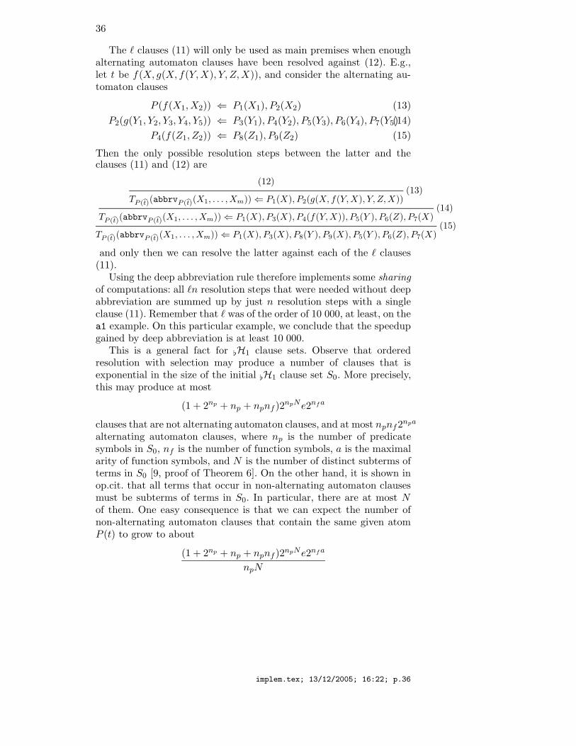
36

The ` clauses (11) will only be used as main premises when enoughalternating automaton clauses have been resolved against (12). E.g.,let t be f(X, g(X, f(Y,X), Y, Z,X)), and consider the alternating au-tomaton clauses

P (f(X1,X2)) ⇐ P1(X1), P2(X2) (13)

P2(g(Y1, Y2, Y3, Y4, Y5)) ⇐ P3(Y1), P4(Y2), P5(Y3), P6(Y4), P7(Y5)(14)

P4(f(Z1, Z2)) ⇐ P8(Z1), P9(Z2) (15)

Then the only possible resolution steps between the latter and theclauses (11) and (12) are

(12)(13)

TP (bt)(abbrvP (bt)(X1, . . . , Xm)) ⇐ P1(X), P2(g(X, f(Y,X), Y, Z,X))(14)

TP (bt)(abbrvP (bt)(X1, . . . , Xm)) ⇐ P1(X), P3(X), P4(f(Y,X)), P5(Y ), P6(Z), P7(X)(15)

TP (bt)(abbrvP (bt)(X1, . . . , Xm)) ⇐ P1(X), P3(X), P8(Y ), P9(X), P5(Y ), P6(Z), P7(X)

and only then we can resolve the latter against each of the ` clauses(11).

Using the deep abbreviation rule therefore implements some sharing

of computations: all `n resolution steps that were needed without deepabbreviation are summed up by just n resolution steps with a singleclause (11). Remember that ` was of the order of 10 000, at least, on thea1 example. On this particular example, we conclude that the speedupgained by deep abbreviation is at least 10 000.

This is a general fact for [H1 clause sets. Observe that orderedresolution with selection may produce a number of clauses that isexponential in the size of the initial [H1 clause set S0. More precisely,this may produce at most

(1 + 2np + np + npnf )2npNe2nfa

clauses that are not alternating automaton clauses, and at most npnf2npa

alternating automaton clauses, where np is the number of predicatesymbols in S0, nf is the number of function symbols, a is the maximalarity of function symbols, and N is the number of distinct subterms ofterms in S0 [9, proof of Theorem 6]. On the other hand, it is shown inop.cit. that all terms that occur in non-alternating automaton clausesmust be subterms of terms in S0. In particular, there are at most Nof them. One easy consequence is that we can expect the number ofnon-alternating automaton clauses that contain the same given atomP (t) to grow to about

(1 + 2np + np + npnf )2npNe2nfa

npN

implem.tex; 13/12/2005; 16:22; p.36

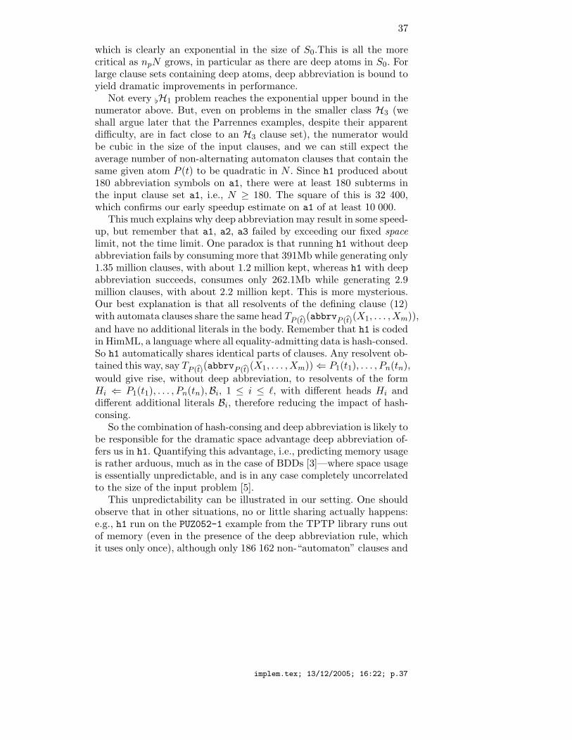
37

which is clearly an exponential in the size of S0.This is all the morecritical as npN grows, in particular as there are deep atoms in S0. Forlarge clause sets containing deep atoms, deep abbreviation is bound toyield dramatic improvements in performance.

Not every [H1 problem reaches the exponential upper bound in thenumerator above. But, even on problems in the smaller class H3 (weshall argue later that the Parrennes examples, despite their apparentdifficulty, are in fact close to an H3 clause set), the numerator wouldbe cubic in the size of the input clauses, and we can still expect theaverage number of non-alternating automaton clauses that contain thesame given atom P (t) to be quadratic in N . Since h1 produced about180 abbreviation symbols on a1, there were at least 180 subterms inthe input clause set a1, i.e., N ≥ 180. The square of this is 32 400,which confirms our early speedup estimate on a1 of at least 10 000.

This much explains why deep abbreviation may result in some speed-up, but remember that a1, a2, a3 failed by exceeding our fixed space

limit, not the time limit. One paradox is that running h1 without deepabbreviation fails by consuming more that 391Mb while generating only1.35 million clauses, with about 1.2 million kept, whereas h1 with deepabbreviation succeeds, consumes only 262.1Mb while generating 2.9million clauses, with about 2.2 million kept. This is more mysterious.Our best explanation is that all resolvents of the defining clause (12)with automata clauses share the same head TP (bt)(abbrvP (bt)(X1, . . . ,Xm)),

and have no additional literals in the body. Remember that h1 is codedin HimML, a language where all equality-admitting data is hash-consed.So h1 automatically shares identical parts of clauses. Any resolvent ob-tained this way, say TP (bt)(abbrvP (bt)(X1, . . . ,Xm)) ⇐ P1(t1), . . . , Pn(tn),

would give rise, without deep abbreviation, to resolvents of the formHi ⇐ P1(t1), . . . , Pn(tn),Bi, 1 ≤ i ≤ `, with different heads Hi anddifferent additional literals Bi, therefore reducing the impact of hash-consing.

So the combination of hash-consing and deep abbreviation is likely tobe responsible for the dramatic space advantage deep abbreviation of-fers us in h1. Quantifying this advantage, i.e., predicting memory usageis rather arduous, much as in the case of BDDs [3]—where space usageis essentially unpredictable, and is in any case completely uncorrelatedto the size of the input problem [5].

This unpredictability can be illustrated in our setting. One shouldobserve that in other situations, no or little sharing actually happens:e.g., h1 run on the PUZ052-1 example from the TPTP library runs outof memory (even in the presence of the deep abbreviation rule, whichit uses only once), although only 186 162 non-“automaton” clauses and

implem.tex; 13/12/2005; 16:22; p.37

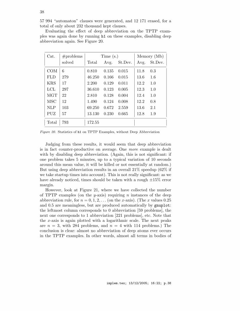
38

57 994 “automaton” clauses were generated, and 12 171 erased, for atotal of only about 232 thousand kept clauses.

Evaluating the effect of deep abbreviation on the TPTP exam-ples was again done by running h1 on these examples, disabling deepabbreviation again. See Figure 20.



COM 6 0.810 0.135 0.015 11.8 0.3

FLD 279 46.250 0.166 0.015 13.6 1.6

KRS 17 2.200 0.129 0.011 12.2 1.0

LCL 297 36.610 0.123 0.005 12.3 1.0

MGT 22 2.810 0.128 0.004 12.4 1.0

MSC 12 1.490 0.124 0.008 12.2 0.8

NLP 103 69.250 0.672 2.559 13.6 2.1

PUZ 57 13.130 0.230 0.665 12.8 1.9

Total 793 172.55

Figure 20. Statistics of h1 on TPTP Examples, without Deep Abbreviation

Judging from these results, it would seem that deep abbreviationis in fact counter-productive on average. One more example is dealtwith by disabling deep abbreviation. (Again, this is not significant: ifone problem takes 5 minutes, up to a typical variation of 10 secondsaround this mean value, it will be killed or not essentially at random.)But using deep abbreviation results in an overall 21% speedup (62% ifwe take startup times into account). This is not really significant: as wehave already noticed, times should be taken with a rough ±15% errormargin.

However, look at Figure 21, where we have collected the numberof TPTP examples (on the y-axis) requiring n instances of the deepabbreviation rule, for n = 0, 1, 2, . . . (on the x-axis). (The x values 0.25and 0.5 are meaningless, but are produced automatically by gnuplot:the leftmost column corresponds to 0 abbreviation [59 problems], thenext one corresponds to 1 abbreviation [221 problems], etc. Note thatthe x-axis is again plotted with a logarithmic scale. The next peaksare n = 3, with 284 problems, and n = 4 with 114 problems.) Theconclusion is clear: almost no abbreviation of deep atoms ever occursin the TPTP examples. In other words, almost all terms in bodies of

implem.tex; 13/12/2005; 16:22; p.38

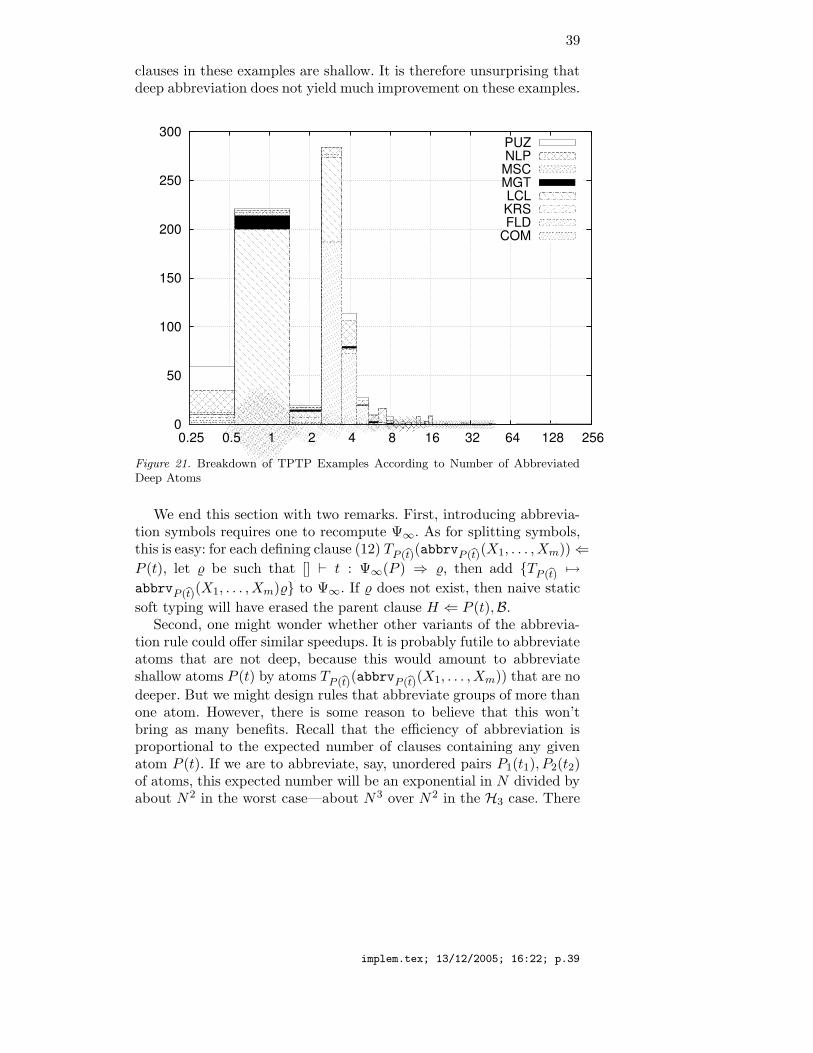
39

clauses in these examples are shallow. It is therefore unsurprising thatdeep abbreviation does not yield much improvement on these examples.

0

50

100

150

200

250

300

0.25 0.5 1 2 4 8 16 32 64 128 256


COM

Figure 21. Breakdown of TPTP Examples According to Number of AbbreviatedDeep Atoms

We end this section with two remarks. First, introducing abbrevia-tion symbols requires one to recompute Ψ∞. As for splitting symbols,this is easy: for each defining clause (12) TP (bt)(abbrvP (bt)(X1, . . . ,Xm)) ⇐

P (t), let % be such that [] ` t : Ψ∞(P ) ⇒ %, then add TP (bt) 7→

abbrvP (bt)(X1, . . . ,Xm)% to Ψ∞. If % does not exist, then naive static

soft typing will have erased the parent clause H ⇐ P (t),B.Second, one might wonder whether other variants of the abbrevia-

tion rule could offer similar speedups. It is probably futile to abbreviateatoms that are not deep, because this would amount to abbreviateshallow atoms P (t) by atoms TP (bt)(abbrvP (bt)(X1, . . . ,Xm)) that are no

deeper. But we might design rules that abbreviate groups of more thanone atom. However, there is some reason to believe that this won’tbring as many benefits. Recall that the efficiency of abbreviation isproportional to the expected number of clauses containing any givenatom P (t). If we are to abbreviate, say, unordered pairs P1(t1), P2(t2)of atoms, this expected number will be an exponential in N divided byabout N2 in the worst case—about N 3 over N2 in the H3 case. There

implem.tex; 13/12/2005; 16:22; p.39

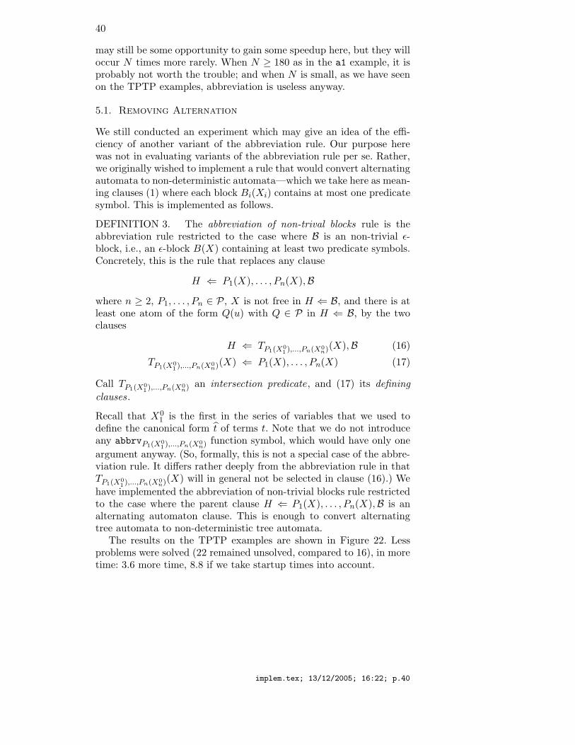
40

may still be some opportunity to gain some speedup here, but they willoccur N times more rarely. When N ≥ 180 as in the a1 example, it isprobably not worth the trouble; and when N is small, as we have seenon the TPTP examples, abbreviation is useless anyway.

5.1. Removing Alternation

We still conducted an experiment which may give an idea of the effi-ciency of another variant of the abbreviation rule. Our purpose herewas not in evaluating variants of the abbreviation rule per se. Rather,we originally wished to implement a rule that would convert alternatingautomata to non-deterministic automata—which we take here as mean-ing clauses (1) where each block Bi(Xi) contains at most one predicatesymbol. This is implemented as follows.

DEFINITION 3. The abbreviation of non-trival blocks rule is theabbreviation rule restricted to the case where B is an non-trivial ε-block, i.e., an ε-block B(X) containing at least two predicate symbols.Concretely, this is the rule that replaces any clause

H ⇐ P1(X), . . . , Pn(X),B

where n ≥ 2, P1, . . . , Pn ∈ P, X is not free in H ⇐ B, and there is atleast one atom of the form Q(u) with Q ∈ P in H ⇐ B, by the twoclauses

H ⇐ TP1(X0

1),...,Pn(X0

n)(X),B (16)

TP1(X0

1),...,Pn(X0

n)(X) ⇐ P1(X), . . . , Pn(X) (17)

Call TP1(X0

1),...,Pn(X0

n) an intersection predicate, and (17) its defining

clauses.

Recall that X01 is the first in the series of variables that we used to

define the canonical form t of terms t. Note that we do not introduceany abbrvP1(X0

1),...,Pn(X0

n) function symbol, which would have only one

argument anyway. (So, formally, this is not a special case of the abbre-viation rule. It differs rather deeply from the abbreviation rule in thatTP1(X0

1),...,Pn(X0

n)(X) will in general not be selected in clause (16).) We

have implemented the abbreviation of non-trivial blocks rule restrictedto the case where the parent clause H ⇐ P1(X), . . . , Pn(X),B is analternating automaton clause. This is enough to convert alternatingtree automata to non-deterministic tree automata.

The results on the TPTP examples are shown in Figure 22. Lessproblems were solved (22 remained unsolved, compared to 16), in moretime: 3.6 more time, 8.8 if we take startup times into account.

implem.tex; 13/12/2005; 16:22; p.40

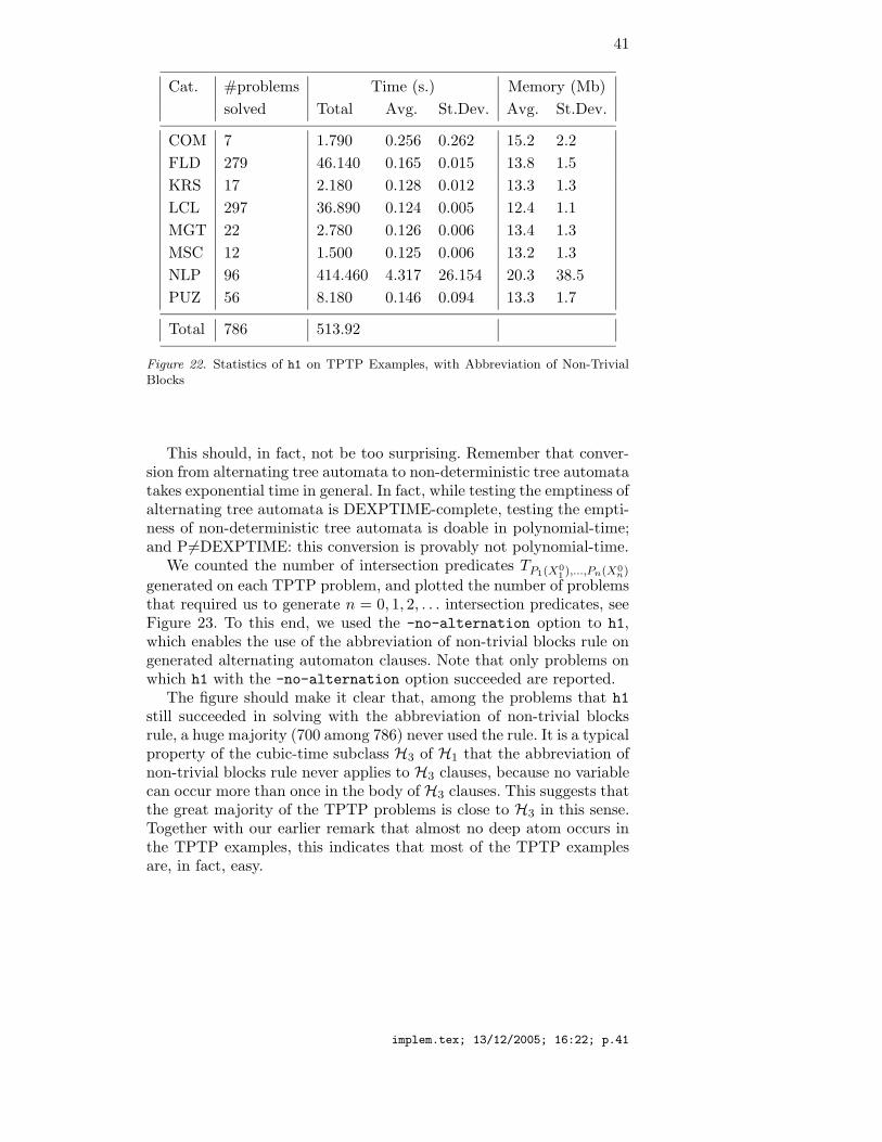
41



COM 7 1.790 0.256 0.262 15.2 2.2

FLD 279 46.140 0.165 0.015 13.8 1.5

KRS 17 2.180 0.128 0.012 13.3 1.3

LCL 297 36.890 0.124 0.005 12.4 1.1

MGT 22 2.780 0.126 0.006 13.4 1.3

MSC 12 1.500 0.125 0.006 13.2 1.3

NLP 96 414.460 4.317 26.154 20.3 38.5

PUZ 56 8.180 0.146 0.094 13.3 1.7

Total 786 513.92

Figure 22. Statistics of h1 on TPTP Examples, with Abbreviation of Non-TrivialBlocks

This should, in fact, not be too surprising. Remember that conver-sion from alternating tree automata to non-deterministic tree automatatakes exponential time in general. In fact, while testing the emptiness ofalternating tree automata is DEXPTIME-complete, testing the empti-ness of non-deterministic tree automata is doable in polynomial-time;and P6=DEXPTIME: this conversion is provably not polynomial-time.

We counted the number of intersection predicates TP1(X0

1),...,Pn(X0

n)

generated on each TPTP problem, and plotted the number of problemsthat required us to generate n = 0, 1, 2, . . . intersection predicates, seeFigure 23. To this end, we used the -no-alternation option to h1,which enables the use of the abbreviation of non-trivial blocks rule ongenerated alternating automaton clauses. Note that only problems onwhich h1 with the -no-alternation option succeeded are reported.

The figure should make it clear that, among the problems that h1

still succeeded in solving with the abbreviation of non-trivial blocksrule, a huge majority (700 among 786) never used the rule. It is a typicalproperty of the cubic-time subclass H3 of H1 that the abbreviation ofnon-trivial blocks rule never applies to H3 clauses, because no variablecan occur more than once in the body of H3 clauses. This suggests thatthe great majority of the TPTP problems is close to H3 in this sense.Together with our earlier remark that almost no deep atom occurs inthe TPTP examples, this indicates that most of the TPTP examplesare, in fact, easy.

implem.tex; 13/12/2005; 16:22; p.41

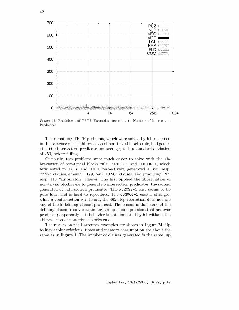
42

0

100

200

300

400

500

600

700

1 4 16 64 256 1024


COM

Figure 23. Breakdown of TPTP Examples According to Number of IntersectionPredicates

The remaining TPTP problems, which were solved by h1 but failedin the presence of the abbreviation of non-trivial blocks rule, had gener-ated 600 intersection predicates on average, with a standard deviationof 250, before failing.

Curiously, two problems were much easier to solve with the ab-breviation of non-trivial blocks rule, PUZ038-1 and COM006-1, whichterminated in 0.8 s. and 0.9 s. respectively, generated 4 325, resp.22 924 clauses, erasing 1 179, resp. 10 904 clauses, and producing 197,resp. 110 “automaton” clauses. The first applied the abbreviation ofnon-trivial blocks rule to generate 5 intersection predicates, the secondgenerated 62 intersection predicates. The PUZ038-1 case seems to bepure luck, and is hard to reproduce. The COM006-1 case is stranger:while a contradiction was found, the 462 step refutation does not useany of the 5 defining clauses produced. The reason is that none of thedefining clauses resolves again any group of side premises that are everproduced; apparently this behavior is not simulated by h1 without theabbreviation of non-trivial blocks rule.

The results on the Parrennes examples are shown in Figure 24. Upto inevitable variations, times and memory consumption are about thesame as in Figure 1. The number of clauses generated is the same, up

implem.tex; 13/12/2005; 16:22; p.42

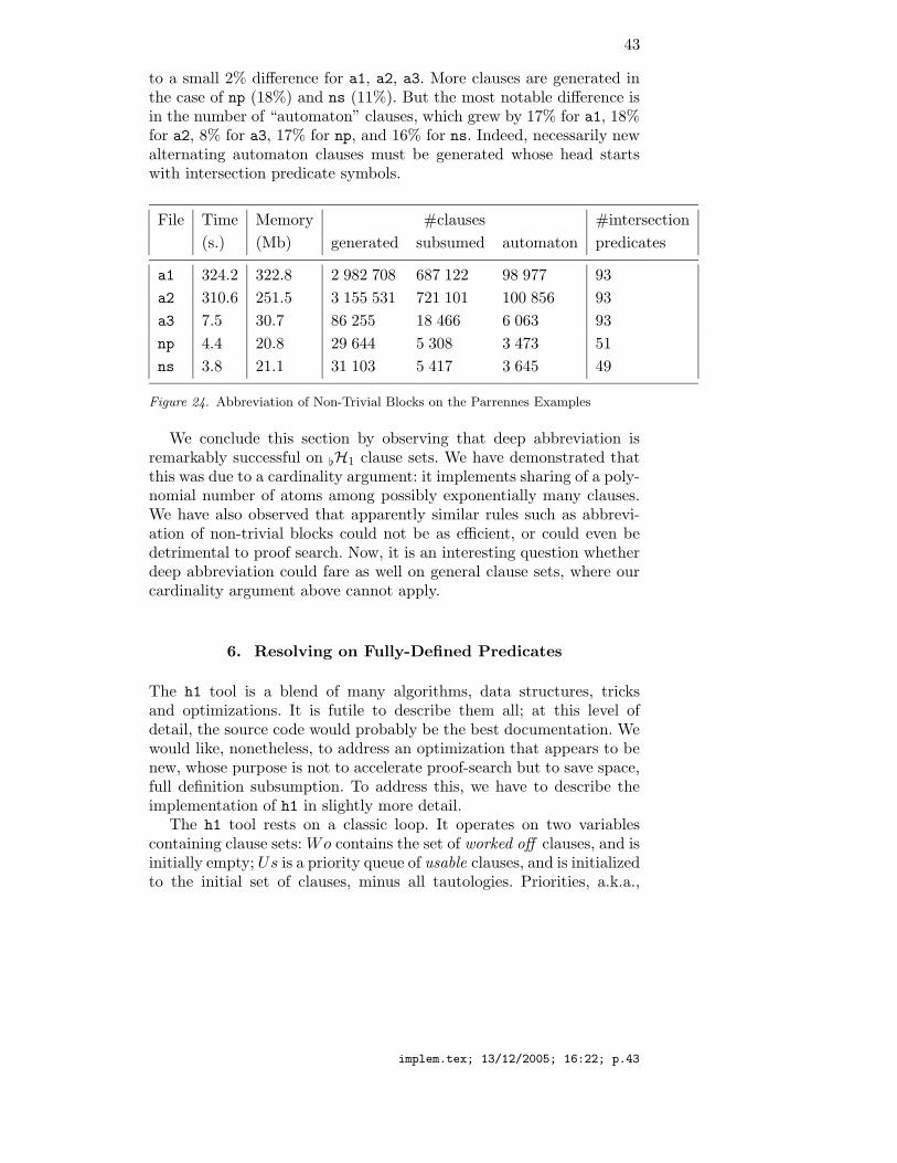
43

to a small 2% difference for a1, a2, a3. More clauses are generated inthe case of np (18%) and ns (11%). But the most notable difference isin the number of “automaton” clauses, which grew by 17% for a1, 18%for a2, 8% for a3, 17% for np, and 16% for ns. Indeed, necessarily newalternating automaton clauses must be generated whose head startswith intersection predicate symbols.

File Time Memory #clauses #intersection

(s.) (Mb) generated subsumed automaton predicates

a1 324.2 322.8 2 982 708 687 122 98 977 93

a2 310.6 251.5 3 155 531 721 101 100 856 93

a3 7.5 30.7 86 255 18 466 6 063 93

np 4.4 20.8 29 644 5 308 3 473 51

ns 3.8 21.1 31 103 5 417 3 645 49

Figure 24. Abbreviation of Non-Trivial Blocks on the Parrennes Examples

We conclude this section by observing that deep abbreviation isremarkably successful on [H1 clause sets. We have demonstrated thatthis was due to a cardinality argument: it implements sharing of a poly-nomial number of atoms among possibly exponentially many clauses.We have also observed that apparently similar rules such as abbrevi-ation of non-trivial blocks could not be as efficient, or could even bedetrimental to proof search. Now, it is an interesting question whetherdeep abbreviation could fare as well on general clause sets, where ourcardinality argument above cannot apply.

6. Resolving on Fully-Defined Predicates

The h1 tool is a blend of many algorithms, data structures, tricksand optimizations. It is futile to describe them all; at this level ofdetail, the source code would probably be the best documentation. Wewould like, nonetheless, to address an optimization that appears to benew, whose purpose is not to accelerate proof-search but to save space,full definition subsumption. To address this, we have to describe theimplementation of h1 in slightly more detail.

The h1 tool rests on a classic loop. It operates on two variablescontaining clause sets: Wo contains the set of worked off clauses, and isinitially empty; Us is a priority queue of usable clauses, and is initializedto the initial set of clauses, minus all tautologies. Priorities, a.k.a.,

implem.tex; 13/12/2005; 16:22; p.43

44

weights, are assigned to each clause in Us so that clauses with smallestweights are selected first.

The basic loop—not quite the h1 loop, but close—works as thefollowing pseudo-code (we use “resolvent” to mean the conclusion ofthe ordered resolution with selection rule):

1.while Us 6= ∅ 2. pick some clause C with smallest weight from Us,3. and remove it from Us;4. if C is the empty clause ⊥ then return “Unsatisfiable”;5. if C is subsumed by some clause from Wo then continue;6. remove all clauses subsumed by C from Wo;7. for each resolvent C ′ of C with some clauses in Wo,8. for each clause H ⇐ B obtained from C ′ by ε-splitting

and deep abbreviation,9. if H ⇐ B is not a tautology

10. and Ψ∞ B ⇒ % for some %11. then add H ⇐ B to Us;12. add C to Wo;13.14.return “Satisfiable”;

This loop is relatively naive by today’s standards. E.g., no clause in Usis ever removed before it is picked at line 2, or is ever used to subsumethe clause C gotten at line 2.

The weight assigned to C when it is inserted into Wo at line 12 issimple, and the result of trial and error: alternating automaton clauseshave weight 0, goal clauses ⊥ ⇐ B are assigned weight 1, clauses ofthe form qB ⇐ B, where qB is a splitting symbol, and clauses whosebody contain some splitting symbol, get weight 2; clauses whose headstarts with an abbreviation symbol TP (bt) have weight 3; clauses of the

form P (X) ⇐ B have weight 4. The weight of all other clauses H ⇐ Bis 4 plus the size of the body B. This reflects the order in which weprefer to consider each kind of clause. However, this is again rathernaive by today’s standards. In particular, we only select clauses byweight, not depth. This is also far from the sophistication displayed inrecent studies [19]. However, remember our goal here is not so much incompetitive testing (see Section 1.1).

One improvement to the above algorithm, implemented in h1, re-places line 12 by: add C to Wo if C is not strictly subsumed by any ofthe clauses H ⇐ B added to Us at line 11. This implements a form ofresolution subsumption, see [2].

At any given stage of this algorithm, say that a predicate symbol Pis fully defined if and only if all “automaton” clauses with head starting

implem.tex; 13/12/2005; 16:22; p.44

45

with P that will ever be produced are already in Wo. In other words, ifand only if P (X) will not be added later to Wo, nor any alterating au-tomaton clause of the form P (f(X1, . . . ,Xk)) ⇐ B1(X1), . . . , Bk(Xk).This can be estimated as follows. Maintain an additional table ∆,mapping each predicate symbol P to the number of clauses of theform P (t) ⇐ B for some t and B, that lie in Us, or that are in Wobut are neither alternating automaton nor universal clauses. It is easyin principle (although it is hard to implement without bugs, in ourexperience) to maintain these counts, by a reference counting stylealgorithm. If ∆(P ) drops to 0, then P is fully defined.

The point in fully defined symbols is that they arise naturally fromthe approximation procedure of Section 3.2. The predicate symbol Qin rule (7), notably, will be classified as fully defined as soon as thedefining clause Q(t) ⇐ B is picked at line 2. This is natural: Q(t) isindeed completely defined by the latter clause, as an abbreviation forB. The deep abbreviation symbols TP (bt) will also profit from this rule,

at some later time.Assume that P is fully defined. If the clause C picked at line 2 is

of the form H0 ⇐ P (t0),B0 where P (t0) is selected, then (assuming,for the sake of simplicity, that we resolve on P (t) only, amongst allpossible atoms in the body P (t0),B0) all the resolvents between C asmain premise and side premises P (ti) ⇐ Bi (which must be universalor alternating automaton clauses) that will ever be generated must begenerated at line 7, and not at any later turn of the loop. We cantherefore remove C after lines 7-11; in other words, in this case, wedo not add C to Wo at line 12. We call this removal rule straight full

definition subsumption.There is another, symmetric case where knowing that P is fully

defined helps, namely when C at line 2 is the last “automaton” clauseto consider before P is fully defined. Formally, when ∆(P ) = 1 justbefore line 2, where C is an “automaton” clause with a head of theform P (s) for some s. Then all the clauses H0 ⇐ P (t0),B0 againstwhich C will be resolved at line 7 can be removed from Wo. Call thisremoval rule backward full definition subsumption.

We go a bit further, and choose to resolve on atoms starting with afully defined symbol prioritarily. In other words, we exploit the freedomin the definition of the selection function that we had observed inSection 3.1. Here is the real definition of our selection function, in thecase 2. where the body B of the given clause contains at least some non-simple atom: if some non-simple atom P (t) in B is such that P is fullydefined, then select all non-simple atoms P (t) with P fully defined fromB; otherwise, select all non-simple atoms from B. This is implementedin h1.

implem.tex; 13/12/2005; 16:22; p.45

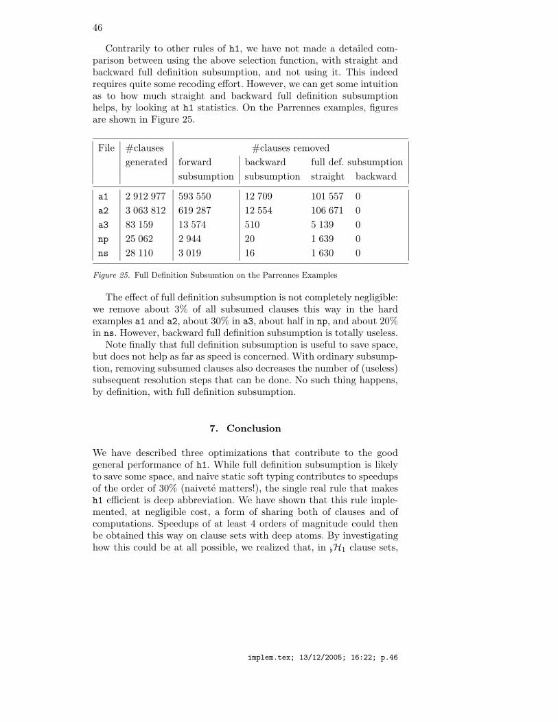
46

Contrarily to other rules of h1, we have not made a detailed com-parison between using the above selection function, with straight andbackward full definition subsumption, and not using it. This indeedrequires quite some recoding effort. However, we can get some intuitionas to how much straight and backward full definition subsumptionhelps, by looking at h1 statistics. On the Parrennes examples, figuresare shown in Figure 25.

File #clauses #clauses removed

generated forward backward full def. subsumption

subsumption subsumption straight backward

a1 2 912 977 593 550 12 709 101 557 0

a2 3 063 812 619 287 12 554 106 671 0

a3 83 159 13 574 510 5 139 0

np 25 062 2 944 20 1 639 0

ns 28 110 3 019 16 1 630 0

Figure 25. Full Definition Subsumtion on the Parrennes Examples

The effect of full definition subsumption is not completely negligible:we remove about 3% of all subsumed clauses this way in the hardexamples a1 and a2, about 30% in a3, about half in np, and about 20%in ns. However, backward full definition subsumption is totally useless.

Note finally that full definition subsumption is useful to save space,but does not help as far as speed is concerned. With ordinary subsump-tion, removing subsumed clauses also decreases the number of (useless)subsequent resolution steps that can be done. No such thing happens,by definition, with full definition subsumption.

7. Conclusion

We have described three optimizations that contribute to the goodgeneral performance of h1. While full definition subsumption is likelyto save some space, and naive static soft typing contributes to speedupsof the order of 30% (naivete matters!), the single real rule that makesh1 efficient is deep abbreviation. We have shown that this rule imple-mented, at negligible cost, a form of sharing both of clauses and ofcomputations. Speedups of at least 4 orders of magnitude could thenbe obtained this way on clause sets with deep atoms. By investigatinghow this could be at all possible, we realized that, in [H1 clause sets,

implem.tex; 13/12/2005; 16:22; p.46

47

only polynomially many atoms could ever be produced, but up to anexponential number of clauses could be generated. Consequently, someatoms must be shared in the proportion of an exponential divided bya polynomial. While this is true for [H1, it is an interesting ques-tion whether a similar phenomenon is bound to happen on generalfirst-order clause sets, and whether deep abbreviation would profit togeneral-purpose theorem provers.

Acknowledgements.

We wish to thank Helmut Seidl for several interesting discussions,Julien Olivain for raising the question of the interaction of deep abbre-viation with memory consumption, and Fabrice Parrennes for providingthe clause sets mentioned in the paper.

References

1. M. Abadi and A. D. Gordon. A calculus for cryptographic protocols: Thespi calculus. In Fourth ACM Conference on Computer and CommunicationsSecurity. ACM Press, 1997.

2. L. Bachmair and H. Ganzinger. Resolution theorem proving. In J. A. Robin-son and A. Voronkov, editors, Handbook of Automated Reasoning, volume I,chapter 2, pages 19–99. North-Holland, 2001.

3. R. E. Bryant. Graph-based algorithms for boolean functions manipulation.IEEE Trans. Comp., C35(8):677–692, 1986.

4. K. Claessen and N. Sorensson. New techniques that improve MACE-style finitemodel building. Proc. CADE-19 Workshop W4, July 2003.

5. O. Coudert. SIAM : Une Boıte a Outils Pour la Preuve Formelle de SystemesSequentiels. PhD thesis, Ecole Nationale Superieure des Telecommunications,Paris, Oct. 1991.

6. T. Fruhwirth, E. Shapiro, M. Y. Vardi, and E. Yardeni. Logic programs astypes for logic programs. In Proc. 6th Symp. Logic in Computer Science, pages300–309. IEEE Computer Society Press, 1991.

7. E. Goto. Monocopy and associative algorithms in an extended Lisp. Technicalreport, U. Tokyo, 1974.

8. J. Goubault-Larrecq. HimML: Standard ML with fast sets and maps. InProc. 5th ACM SIGPLAN Workshop on Standard ML and its Applications(ML’94), pages 62–69, Orlando, Florida, USA, 1994. Implementation availableon http://www.lsv.ens-cachan.fr/∼goubault/himml-dwnld.html.

9. J. Goubault-Larrecq. Deciding H1 by resolution. Information ProcessingLetters, 95(3):401–408, Aug. 2005.

10. J. Goubault-Larrecq. Determinization and models. Information ProcessingLetters, 2006. Submitted.

11. J. Goubault-Larrecq and F. Parrennes. Cryptographic protocol analysis on realC code. In R. Cousot, editor, Proceedings of the 6th International Conference on

implem.tex; 13/12/2005; 16:22; p.47

48

Verification, Model Checking and Abstract Interpretation (VMCAI’05), Paris,France, Jan. 2005. Springer-Verlag LNCS 3385.

12. J. N. Hooker. Testing heuristics: We have it all wrong. Journal of Heuristics,1:33–42, 1996.

13. F. Jacquemard, M. Rusinowitch, and L. Vigneron. Tree automata with equalityconstraints modulo equational theories. Research report, INRIA Futurs, 2005.

14. S. Limet and G. Salzer. Manipulating tree tuple languages by trans-forming logic programs. Electronic Notes in Theoretical Computer Sci-ence, 86(1), 2003. Proceedings of the 4th Intl. Workshop on First-OrderTheorem Proving (FTP’2003), Valencia, Spain, June 2003. Long version,LIFO Research Report RR-2004-01, March 2004, Orleans, France, avail-able from http://www.univ-orleans.fr/SCIENCES/LIFO/prodsci/rapports/

RR/RR2004/RR-2004-01.ps.gz.15. R. M. Needham and M. D. Schroeder. Using encryption for authentication in

large networks of computers. Communications of the ACM, 21(12):993–999,1978.

16. F. Nielson, H. R. Nielson, and H. Seidl. Normalizable Horn clauses, stronglyrecognizable relations and Spi. In Proc. 9th Static Analysis Symposium, pages20–35. Springer Verlag LNCS 2477, 2002.

17. A. Pettorossi and M. Proietti. Transformation of logic programs. In D. Gabbay,C. Hogger, and J. Robinson, editors, Handbook of Logic in Artificial Intelligenceand Logic Programming, volume 5, pages 697–787. Oxford University Press,1998.

18. A. Riazanov and A. Voronkov. Splitting without backtracking. In B. Nebel,editor, Proc. 17th Intl. Joint Conf. Artificial Intelligence, volume 1, pages 611–617. Morgan Kaufmann, Aug. 2001.

19. A. Riazanov and A. Voronkov. Limited resource strategy in resolution theoremproving. Journal of Symbolic Computation, 36(1-2):101–115, July 2003.

20. G. Sutcliffe and C. B. Suttner. The TPTP problem library: CNF release v1.2.1.Journal of Automated Reasoning, 21(2):177–203, 1998.

21. T. Tammet. Finite model building: Improvements and comparisons. Proc.CADE-19 Workshop W4, July 2003.

22. C. Weidenbach. Computational Aspects of a First-Order Logic with Sorts.PhD thesis, Technische Fakultat der Universitat des Saarlandes, Saarbrucken,Germany, 1996.

23. C. Weidenbach. Sorted unification and tree automata. In W. Bibel andP. Schmitt, editors, Applied Logic, volume 1, chapter 9, pages 291–320. Kluwer,1998.

24. C. Weidenbach. Towards an automatic analysis of security protocols in first-order logic. In Proc. 16th Intl. Conf. Automated Deduction, pages 314–328.Springer-Verlag LNAI 1632, 1999.

25. C. Weidenbach, U. Brahm, T. Hillenbrand, E. Keen, C. Theobald, andD. Topic. SPASS version 2.0. In A. Voronkov, editor, Proceedings of the18th International Conference on Automated Deduction. Springer-Verlag LNAI2392, 2002.

26. C. Weidenbach, B. Gaede, and G. Rock. SPASS & FLOTTER version 0.42. InM. A. McRobbie and J. K. Slaney, editors, Proc. 13th Intl. Conf. AutomatedDeduction, pages 141–145. Springer-Verlag LNCS 1104, 1996.

Address for Offprints: ENS Cachan61 avenue du president-Wilson,F-94235 Cachan Cedex

implem.tex; 13/12/2005; 16:22; p.48

Implementing H1 by Resolution

Documents