Implementing Bilateral Tariff Rate Quotas in GTAP using ...

Implementing Bilateral Tariff Rate Quotasin GTAP using GEMPACK

Aziz Elbehri and K.R. Pearson

GTAP Technical Paper No. 18

December 2000

Aziz Elbehri, Markets and Trade Economics Division, USDA/ERS, 1800 M St., NW,Washington, DC 20036, USA. [email protected]

Ken Pearson, Centre of Policy Studies and Impact Project, Monash University, Clayton Vic3800, Australia. [email protected]

Abstract

Explicit modelling of tariff rate quotas (TRQs) is important in the current World TradeOrganization negotiations. In order to do such modelling with GTAP, extra data is requiredand extra equations must be added to the model. This paper provides tools for assistingmodellers to carry out explicit modelling of bilateral tariff rate quotas in GTAP usingGEMPACK.

The paper describes how the extra data for sugar TRQ applications was obtained andreconciled with the standard GTAP data. Supplied with the paper is a TABLO Input fileTRQDATA.TAB which others can use for reconciling their TRQ data with the usual GTAPdata.

Supplied with the paper is a module which can be added to the standard TABLO Input files forGTAP. This module contains the extra equations required to model TRQs.

Detailed hands-on examples are supplied with the paper, as is a TRQ application relating toliberalization of TRQs on sugar imported into the USA. Readers of the paper can replicatethese applications.

A windows interface TRQmate is supplied with the paper. This is a relatively general-purposeinterface which automates the steps in carrying out TRQ applications with GTAP andGEMPACK.

If you wish to carry out your own bilateral TRQ applications with GTAP and GEMPACK, thetools supplied with this paper will make it relatively straightforward for you to do so once youhave collected the extra data you need.

1 INTRODUCTION.......................................................................................1

2 ECONOMICS OF TRQ REGIME: A GRAPHICAL EXPOSITION.............3

3 THE TRQ EQUATIONS IN GTAP/GEMPACK NOTATION......................5

3.1 GTAP Notation : New TRQ Variables and Equations........................................................63.1.1 TRQ TABLO Input Files GTAPxTRQ.TAB...................................................................9

3.2 Extra Data Required for GTAPxTRQ.TAB......................................................................103.2.1 Extra Data in the TRQ Module in GTAPxTRQ.TAB ....................................................11

3.3 Collecting and Processing Extra TRQ Data – TRQDATA.TAB.......................................123.3.1 Some Steps in TRQDATA.TAB...................................................................................133.3.2 The 4-commodity, 6-region Data Used in the Applications ...........................................14

3.4 Checks on the Extra Data ..................................................................................................15

3.5 Quota Rents........................................................................................................................16

3.6 Reallocating Quota Rent Between Importing and Exporting Regions..............................163.6.1 Extra Data Required for Rent Reallocation ...................................................................173.6.2 Rent Reallocation Data for the Application...................................................................173.6.3 Creating Data Bases with Quota Rents Redistributed ....................................................173.6.4 Obtaining this QRSHARE_X Data...............................................................................183.6.5 Associated Change to EV_ALT in GTAPxTRQ.TAB...................................................18

3.7 Tariff Revenues ..................................................................................................................18

4 GEMPACK PROCEDURES FOR ONE SIMULATION ...........................20

4.1 Overview of the Procedures ...............................................................................................204.1.1 Purpose of the Approximate Simulation .......................................................................204.1.2 Sequence of Calculations .............................................................................................20

4.2 The Command File for the Accurate Simulation...............................................................214.2.1 Solution Method ..........................................................................................................214.2.2 Closure/Shocks section of Command file for Accurate Simulation ................................21

4.3 Automation of These Procedures via TRQmate ................................................................22

4.4 Optional Use of TRQTMS.TAB During a TRQmate Run ................................................23

4.5 The Different TABLO Input F iles Supplied ......................................................................23

5 POLICY APPLICATION: PARTIAL LIBERALIZATION OF SUGAR TRQ25

6 EXAMPLES SUPPLIED..........................................................................28

6.1 Getting Started...................................................................................................................286.1.1 Directory Structure for the Examples............................................................................286.1.2 Processing the TABLO Input Files ...............................................................................28

iv

6.1.3 Making the 6x4 TRQ Data ...........................................................................................29

6.2 Standard Closures..............................................................................................................30

6.3 Introductory Examples ......................................................................................................306.3.1 Reversing these Simulations.........................................................................................32

6.4 Hands-on Guide to Carrying Out These Examples 1-4.....................................................326.4.1 Case 1A in Detail.........................................................................................................336.4.2 Looking at the Results from Case 1A ...........................................................................346.4.3 Doing Case 1B.............................................................................................................356.4.4 Doing Other Examples (Cases 2-4)...............................................................................35

6.5 The Reversal of Case 1A ....................................................................................................36

6.6 Saving the Results of an Application..................................................................................36

6.7 Associated Data-Manipulation TABLO Input Files ..........................................................37

6.8 Checks That Must Be Made After the Accurate Simulation .............................................37

6.9 Example Applications.........................................................................................................386.9.1 Preliminary Redistribution of Quota Rents ...................................................................386.9.2 Running Applications 1-3 ............................................................................................39

6.10 Carrying Out Your Own TRQ Applications .................................................................39

6.11 DECOMP, GTAPVIEW and GTAPVOL......................................................................39

7 OTHER TRQ APPLICATIONS................................................................41

8 REFERENCES........................................................................................42

9 APPENDIX 1 : AGGREGATION OF TRQS............................................43

9.1 Method 1: Aggregation Considering Relative Power of Tariffs ........................................43

9.2 Method 2: Aggregation Considering Quota Rent..............................................................44

9.3 Initializing QXSTRQ_RATIO for an Aggregate TRQ......................................................45

10 APPENDIX 2 : EQUATION E_TMS IN GTAPXTRQ.TAB ......................46

1 Introduction

The tariff-rate quota (TRQ) system emerged from the Uruguay Round Agreement onAgriculture (URAA) as a new policy mechanism that ensures both tariffication and marketaccess. The tariffication consisted of converting non-tariff barriers into tariffs and loweringthose tariffs over a period of time. The URAA also ensured that quantities imported beforethe agreement could continue to be imported--this is the market access side of the Agreement--whereby it was guaranteed that some new quantities were charged duty rates that were notprohibitive. Under the URAA, minimum access was established through the tariff quotasbased either on historical import levels, or a minimum import level representing 3 percent ofdomestic consumption, rising to 5 percent of domestic consumption in 2000. However,minimum access commitments are not guarantees of minimum import levels. They aresimply commitments that no non-tariff barriers (NTBs) will be invoked to prevent imports upto these levels outside the in-quota tariffs.

Since the URAA, tariff rate quota import regime has become widely used for controllingimports of agricultural commodities. The WTO Secretariat reports the total number of tariffquotas equal to 1371 notified by 33 countries. Of these 60 percent of all TRQs are reported byOECD countries and 40 percent by non-OECD countries. While most TRQs are implementedon a global basis, a large number of TRQs are country specific, including many politicallysensitive commodities.

Given the prevalence of TRQs, how to liberalize TRQs will be an important issue in thecurrent WTO negotiations on agricultural market access. There are basically two problemswith the TRQ regime that need to be addressed in the upcoming WTO negotiations: theoverall level of access, and the administration of TRQs (Skully, 1999). Expanded marketaccess will depend on increasing the volume of imports allowed under the current regime ofTRQs, either via expanded minimum access commitments or via lowering out-of quota tariffs.In addition, a variety of methods are used to administer TRQs, resulting either explicitly orimplicitly in quota rents distributed between importers and/or exporters. For country specificTRQs where quota-holding exporters benefit from preferential access, quota rents accrue toexporters and the implications for liberalization is likely to be different for importing vsexporting countries.

Given the importance of TRQs in market access negotiations, quantitative models thataccount for the TRQ mechanism will be an important source of information. During theUruguay Round most quantitative trade policy analyses viewed "policy" in agriculture interms of tax or subsidy equivalents. In other words, observed price differences are taken as agood approximation of the incidence of price or quantity barriers. Hence the modeling of theUruguay Round was usually based on tariff equivalents of various policy measures.However, given the prominence of quotas in the current agricultural policy regime, via TRQs,the modeling of border measures must explicitly come to grips with quantitative restraints.Abbott and Paarlberg (1998) offer a partial equilibrium analysis of the TRQ on pork importsinto the Philippines. This paper develops a TRQ model within a general equilibrium multi-regional context. The proposed model allows for bilateral TRQs and can handle bindingprices, quantity constraints, as well as quota rent reallocations. The main advantage of thisgeneral equilibrium approach is that it provides a more comprehensive vehicle for analyzinginteractions with other aspects of a multilateral trade agreement.

In this paper we describe how bilateral tariff-rate quotas can be implemented for policyanalysis in a GTAP model (Hertel, 1997) using the GEMPACK software (Harrison and

2

Pearson, 1996). This model also allows for endogenous income redistribution based on quotasrent allocation between importers and exporters1.

Supplied in conjunction with the paper is a package of software and files for carrying outTRQ applications with GTAP. This package can be downloaded from the web.In particular the Windows software TRQmate in this package makes it very easy to carry outTRQ applications with GTAP. Detailed instructions relating to this can be found in section 6.

Although we only consider bilateral tariff rate quotas at this point, this modeling frameworkcan be easily extended to include global tariff rate quotas as well. We are considering suchgeneralization in future extensions.

The remainder of the paper is as follow. Section 2 provides a graphical description of theTRQ regime and lays down the theoretical basis for our representation of the TRQ model inGTAP. Section 3 describes in detail the actual code used to implement the TRQ model ofsection 2 using GTAP/GEMPACK terminology. Section 0 describes the GEMPACKprocedure in running the simulations. Section 5 illustrates the model with a policy casescenario involving counterfactual sugar TRQ liberalization2. Section 6 describes the filesassociated with additional examples to run TRQ simulations. This section contains detailedinstructions on how to carry out several hands-on examples of TRQ applications. Section 7contains suggestions on how to carry out your own TRQ applications. Finally, two appendicesare included – the first about aggregating TRQ data and the second a technical appendix aboutthe linearized version of the most complicated non-differentiable equation in the TRQ modulewe added to the standard GTAP TABLO Input file.

Acknowledgements

The authors are grateful to Tom Hertel and Mark Horridge for encouragement, assistance andvital feedback on various aspects of this paper. In particular the methodology used toimplement the inequalities associated with tariff-rate quotas is based on insights given byMark Horridge (Horridge, 1993). The authors are also grateful to Martina Brockmeier andMarkus Lips for reviewing a preliminary draft and providing valuable comments andsuggestions.

1 While we expect that TRQs can be modeled using other software, such as GAMS, we are not awareof any published studies to date that address the TRQ regimes in the context of applied generalequilibrium policy modeling.2 For a full analysis of multi-regional TRQ liberalization in the context of WTO 2000 multilateralnegotiations based on this model, see Elbehri et al. (1999).

3

2 Economics of TRQ regime: a graphical exposition

A tariff rate quota is a trade policy regime, which combines elements of tariffs and quotas.Under the TRQ, imports up to some fixed quantity are subject to a low tariff (in-quota tariff)while imports above that quantity are charged a higher tariff (out-of quota tariffs). In theUruguay Round Agreement on Agriculture these fixed quantities are referred to as minimumaccess commitments.

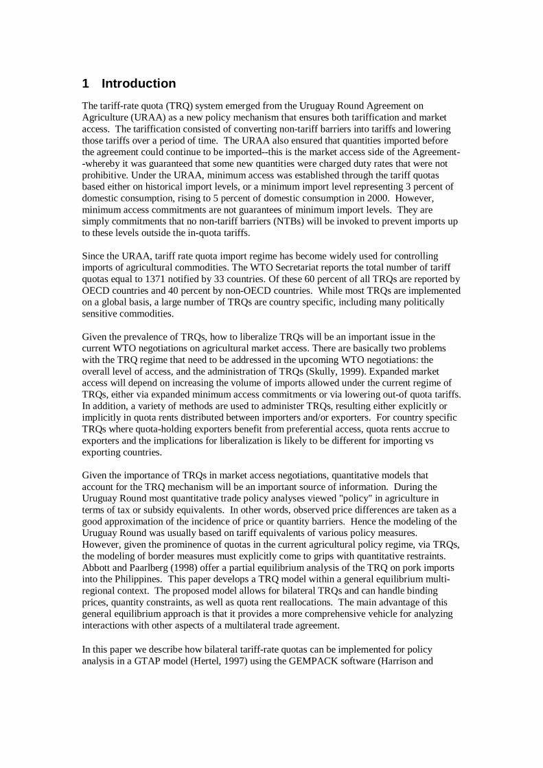
Figure 1 illustrates three possible regimes under the TRQ. Quota (or minimum accesscommitments) is represented by Q. Under the TRQ regime an import supply is represented bya step function with two horizontal lines. The lower line represents the in-quota imports andextends from 0 to Q. The other line represents the effective import supply of over-quotaimports and extends from Q to infinity. At the import volume Q there is a discontinuity: avertical line joins the in-quota and over quota segments. M represents actual imports, whichare determined by a net import demand function, which yields imports according to thedomestic price Pd of the importing country.

In Figure 1, Tin represents the in-quota tariff and Tout the out-of quota tariff. The powers ofthese (1+Tin and 1+Tout respectively) are used in our modeling. [For example, if the in-quota ad valorem rate is 25%, then Tin =0.25 and the power is 1.25.] Pw is the world price andPd is the domestic price determined by the world price plus an applicable tariff. Under theTRQ regime imports can be below the quota Q when in-quota tariff is effective (case 1), orequal to Q making the quota effective (case 2) or above Q making the out-of-quota tariffeffective (case 3). In cases 2 and 3 we have positive quota rents shown in shaded areas,which accrue either to importers, or to exporters, or are shared between importers andexporters, depending on the mechanism by which the TRQ is administered.

In case 1, net import demand at a domestic price equal to the world price times the power ofthe in-quota tariff [Pd = Pw(1 + Tin)] is below the quota Q. The TRQ behaves just like a tariffand no rent accrues. In case 3, net import demand M exceeds the quota Q. In this case Pd =Pw(1 + Tout) and rents are collected by whoever holds the rights to import at the lower in-quotatariff (Tin). Under this regime we have both a rent seeking behavior and an administrativemechanism to allocate the rents. In case 2, net import demand intersects the import supplystep function on its vertical portion at a quantity equal to the quota (Q). In this case thedomestic price exceeds the world price augmented by the in-quota tariff [Pd > Pw(1 + Tin)].The out-of-quota tariff is prohibitive and the difference between Pd and Pw(1 + Tin) representsthe per-unit rent.

The per-unit rent is endogenous and depends on the net import demand intersection with thesupply function. When imports are at quota as in case 2 (Figure 1) the per-unit rent is equal toPd – Pw (1 + Tin). When imports are over quota as in case 3 (Figure 1), the per-unit rent isequal to Pw (Tout – Tin). The total value of the rent is the per-unit rent times the quota volume.

In standard GTAP notation, VIWS denotes the value of imports valued at the world price Pw .In our TRQ treatment, we have found it useful to introduce (see section 3.1 below)

VIWS_TRQ to denote the value of the quota volume Q valued at the world price Pw .VIMSINQ_TRQ to denote the value of the quota volume Q valued at the in-quotaprice Pin .

We show graphically the values of VIWS, VIWS_TRQ and VIMSINQ_TRQ in each case inFigure 1. The shaded areas in cases 2 and 3 of Figure 1 correspond to the quota rent (seesection 3.5 below).

4

Figure 1. Tariff Rate Quota Regime

Imports

P

Q

Pw (1+Tout )

Pd = Pw (1 + Tin )

Imports

P

M=Q

Imports

P

Q

Importdemand

M

Importdemand

M

Case 1: In Quota

Case 2: At Quota

Case 3: Over quota

Pw

Pw

Pw

Pw (1 + Tin )

Pw (1 + Tin )

Pw (1+Tout )

Pd =Pw (1+Tout )

Importdemand

VIWS = bVIWS_TRQ = b+dVIMSINQ_TRQ =a+b+c+d

VIWS = fVIWS_TRQ = fVIMSINQ_TRQ =e+f

e

f

Pd

VIWS = f+gVIWS_TRQ =fVIMSINQ_TRQ =e+f

e

f

ca

b d

g

5

3 The TRQ Equations in GTAP/GEMPACK Notation

Consider imports of some commodity, say sugar, from one region, say Africa, to anotherregion, say USA. If there is a bilateral tariff rate quota in place on these imports, then importsup to a certain volume (the tariff rate quota volume, which we denote by QMS_TRQ) willattract a small tariff (called the in-quota tariff , the power of which we denote by TMSINQ ).Any imports above the tariff rate quota volume QMS_TRQ will attract an extra tariff. Wedistinguish between

• the full extra power of the tariff for over quota imports, which we denote byTMSTRQOVQ , and

• the total power of the tariff for over quota imports, which we denote by TMSOVQ .

Note that

TMSOVQ = TMSTRQOVQ * TMSINQ .

As usual in GTAP, we use TMS to denote the actual power of the import tariff. Here we useTMSTRQ to denote any actual extra power of the tariff (over and above the in-quota tariffTMSINQ). That is,

TMS = TMSINQ * TMSTRQ .

In the notation used in section 2 and Figure 1,

TMSINQ = 1 + Tin ,TMSOVQ = 1 + Tout ,TMSTRQOVQ = (1 + Tout )/(1 + Tin ) ,Pd = Pw * TMS = Pw * TMSINQ * TMSTRQ .

[The standard GTAP notation for Pw and Pd is PIWS and PIMS, respectively.]

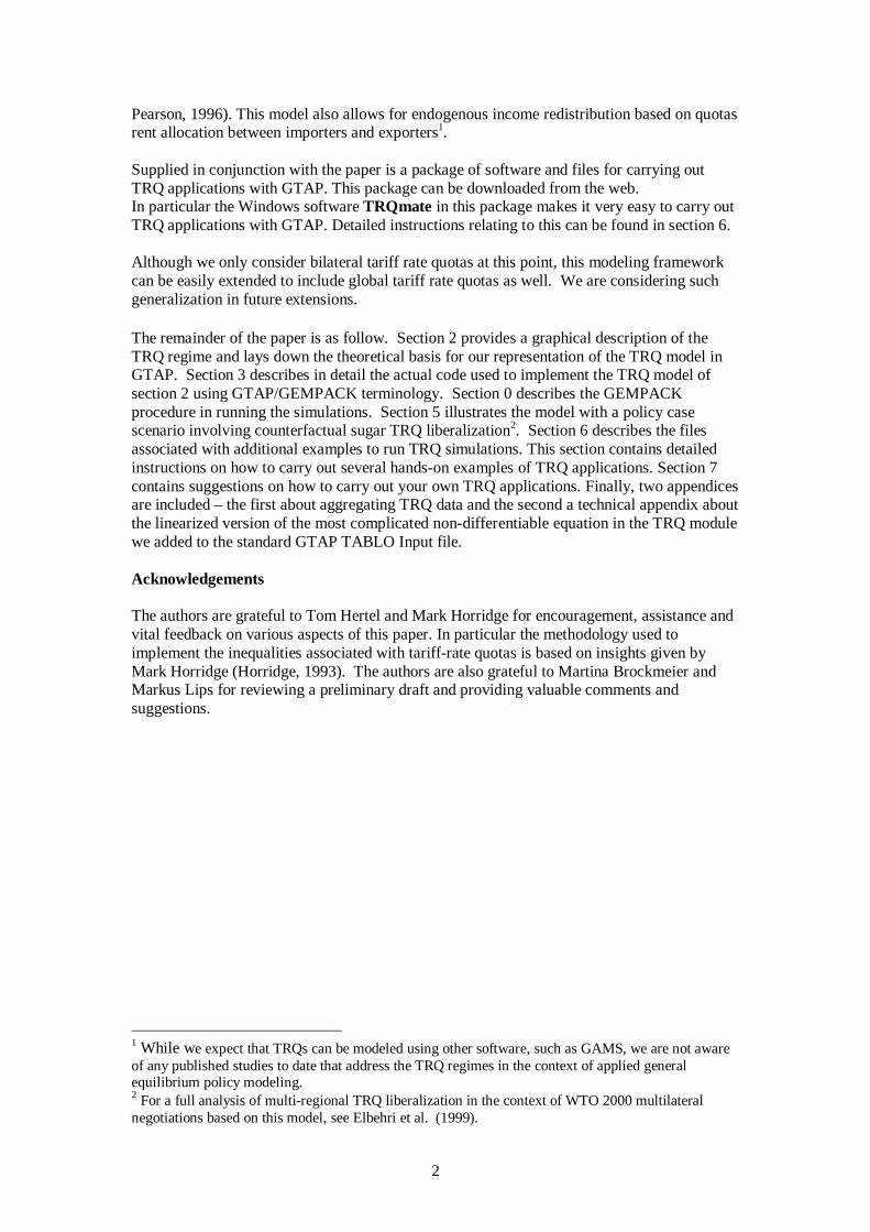
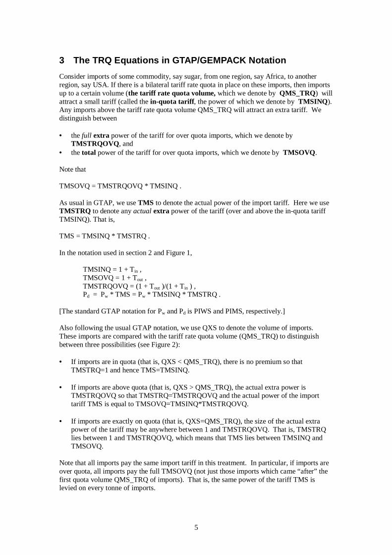
Also following the usual GTAP notation, we use QXS to denote the volume of imports.These imports are compared with the tariff rate quota volume (QMS_TRQ) to distinguishbetween three possibilities (see Figure 2):

• If imports are in quota (that is, QXS < QMS_TRQ), there is no premium so thatTMSTRQ=1 and hence TMS=TMSINQ.

• If imports are above quota (that is, QXS > QMS_TRQ), the actual extra power isTMSTRQOVQ so that TMSTRQ=TMSTRQOVQ and the actual power of the importtariff TMS is equal to TMSOVQ=TMSINQ*TMSTRQOVQ.

• If imports are exactly on quota (that is, QXS=QMS_TRQ), the size of the actual extrapower of the tariff may be anywhere between 1 and TMSTRQOVQ. That is, TMSTRQlies between 1 and TMSTRQOVQ, which means that TMS lies between TMSINQ andTMSOVQ.

Note that all imports pay the same import tariff in this treatment. In particular, if imports areover quota, all imports pay the full TMSOVQ (not just those imports which came “after” thefirst quota volume QMS_TRQ of imports). That is, the same power of the tariff TMS islevied on every tonne of imports.

6

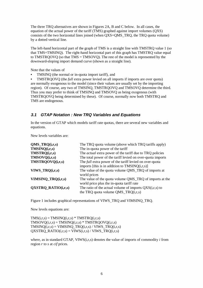
The three TRQ alternatives are shown in Figures 2A, B and C below. In all cases, theequation of the actual power of the tariff (TMS) graphed against import volumes (QXS)consists of the two horizontal lines joined (when QXS=QMS_TRQ, the TRQ quota volume)by a dotted vertical line.

The left-hand horizontal part of the graph of TMS is a straight line with TMSTRQ value 1 (sothat TMS=TMSINQ). The right-hand horizontal part of this graph has TMSTRQ value equalto TMSTRQOVQ (so that TMS = TMSOVQ). The rest of the model is represented by thedownward-sloping import demand curve (shown as a straight line).

Note that the values of• TMSINQ (the normal or in-quota import tariff), and• TMSTRQOVQ (the full extra power levied on all imports if imports are over quota)are normally exogenous to the model (since their values are usually set by the importingregion). Of course, any two of TMSINQ, TMSTRQOVQ and TMSOVQ determine the third.Thus you may prefer to think of TMSINQ and TMSOVQ as being exogenous (withTMSTRQOVQ being determined by these). Of course, normally now both TMSTRQ andTMS are endogenous.

3.1 GTAP Notation : New TRQ Variables and Equations

In the version of GTAP which models tariff rate quotas, there are several new variables andequations.

New levels variables are:

QMS_TRQ(i,r,s) The TRQ quota volume (above which TRQ tariffs apply)TMSINQ(i,r,s) The in-quota power of the tariffTMSTRQ(i,r,s) The actual extra power of the tariff due to TRQ policiesTMSOVQ(i,r,s) The total power of the tariff levied on over-quota importsTMSTRQOVQ(i,r,s) The full extra power of the tariff levied on over-quota

imports [this is in addition to TMSINQ(i,r,s)]VIWS_TRQ(i,r,s) The value of the quota volume QMS_TRQ of imports at

world pricesVIMSINQ_TRQ(i,r,s) The value of the quota volume QMS_TRQ of imports at the

world price plus the in-quota tariff rateQXSTRQ_RATIO(i,r,s) The ratio of the actual volume of imports QXS(i,r,s) to

the TRQ quota volume QMS_TRQ(i,r,s)

Figure 1 includes graphical representations of VIWS_TRQ and VIMSINQ_TRQ.

New levels equations are:

TMS(i,r,s) = TMSINQ(i,r,s) * TMSTRQ(i,r,s)TMSOVQ(i,r,s) = TMSINQ(i,r,s) * TMSTRQOVQ(i,r,s)TMSINQ(i,r,s) = VIMSINQ_TRQ(i,r,s) / VIWS_TRQ(i,r,s)QXSTRQ_RATIO(i,r,s) = VIWS(i,r,s) / VIWS_TRQ(i,r,s)

where, as in standard GTAP, VIWS(i,r,s) denotes the value of imports of commodity i fromregion r to s at cif prices.

7

Imports

TMS=TMSOVQ

Case 3: Over Quota

TMSINQ

TMSOVQ/TMSINQ=TMSTRQOVQ

=TMSTRQ

< QXS

Imports

Importdemand

QMS_TRQ= QXS

TMSOVQ

Case 2: On Quota

TMSINQ

TMSOVQ/TMSINQ=TMSTRQOVQ TMS

TMS/TMSINQ=TMSTRQ

Figure 2: Key variables in the tariff rate quota regime

Power ofthe tarif f

Imports

Importdemand

QMS_TRQ

TMSOVQ

Case 1: In Quota

QXS <

TMS=TMSINQ(here TMSTRQ=1)

TMSOVQ/TMSINQ=TMSTRQOVQ

Power ofthe tariff

Power ofthe tariff

Importdemand

QMS_TRQ

8

The VIWS_TRQ and VIMSINQ_TRQ values are extra data required by this model. Theyare used to infer the value of TMSINQ via the equation above. We say more about this extradata in section 3.2 below.

The main equation describing the TRQ behavior is a little complicated. To introduce it,consider the following IF statements:

(i) If imports are in quota (that is, QXS < QMS_TRQ), we have TMSTRQ(i,r,s)=1 andQXSTRQ_RATIO(i,r,s) < 1.

(ii) If imports are over quota (that is, QXS > QMS_TRQ), we haveTMSTRQ(i,r,s)=TMSTRQOVQ(i,r,s) and QXSTRQ_RATIO(i,r,s) > 1.

(iii) If imports are exactly on quota (that is, QXS = QMS_TRQ), we have TMSTRQ(i,r,s)> 1 and QXSTRQ_RATIO(i,r,s) = 1.

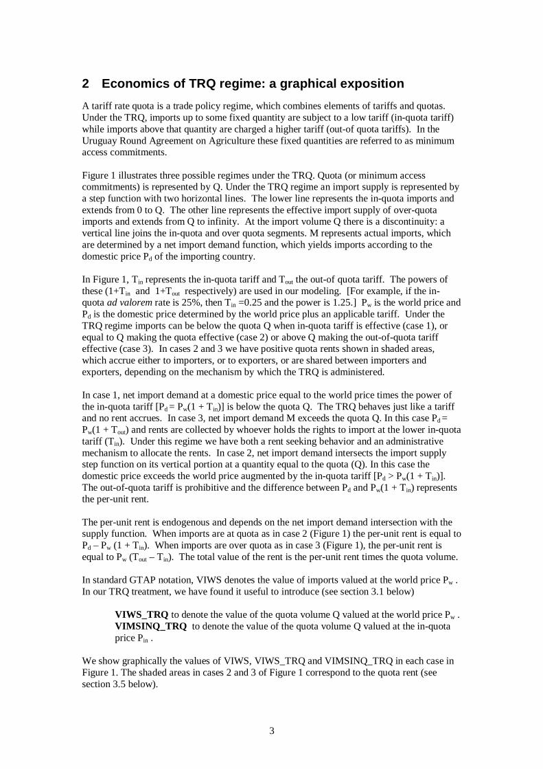
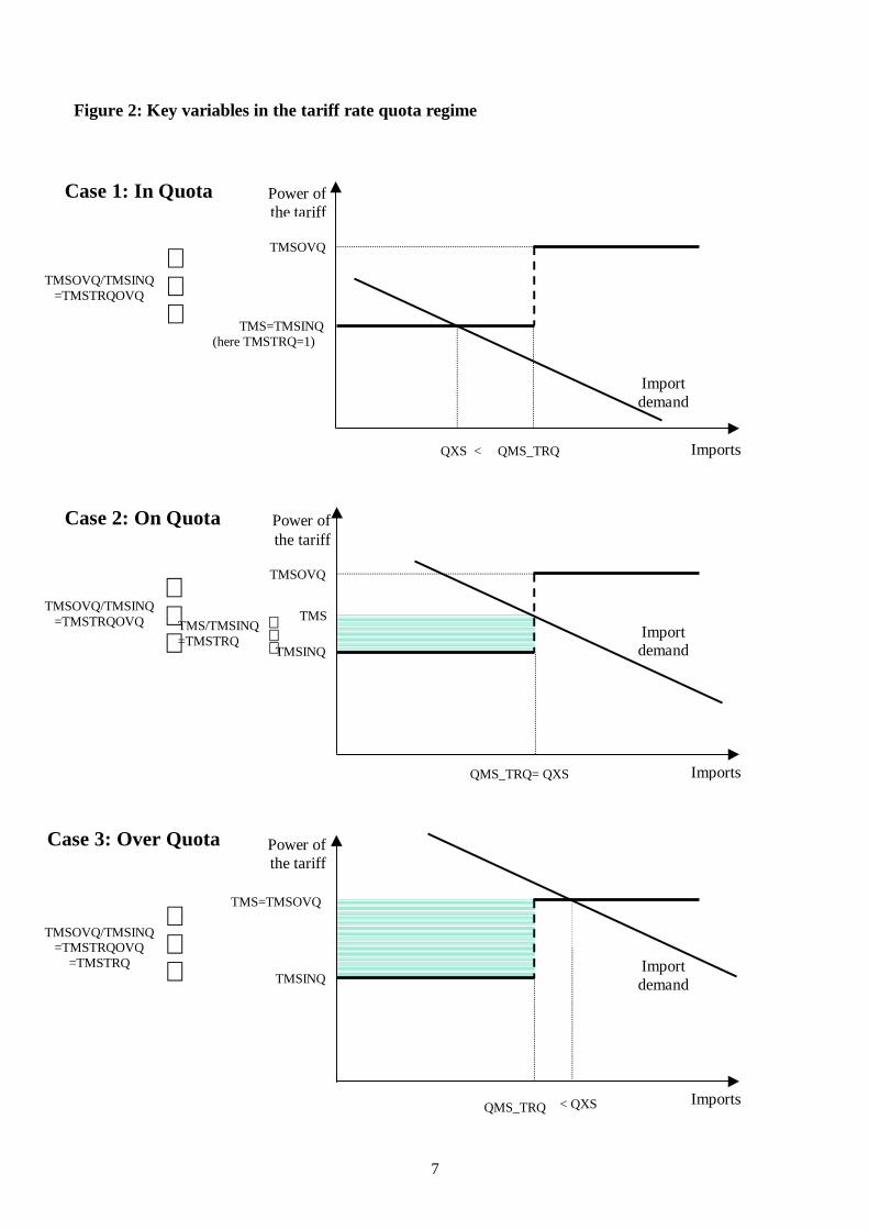
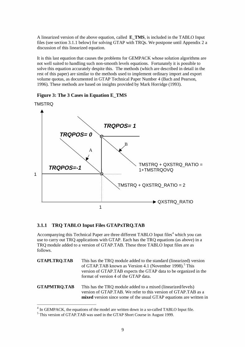
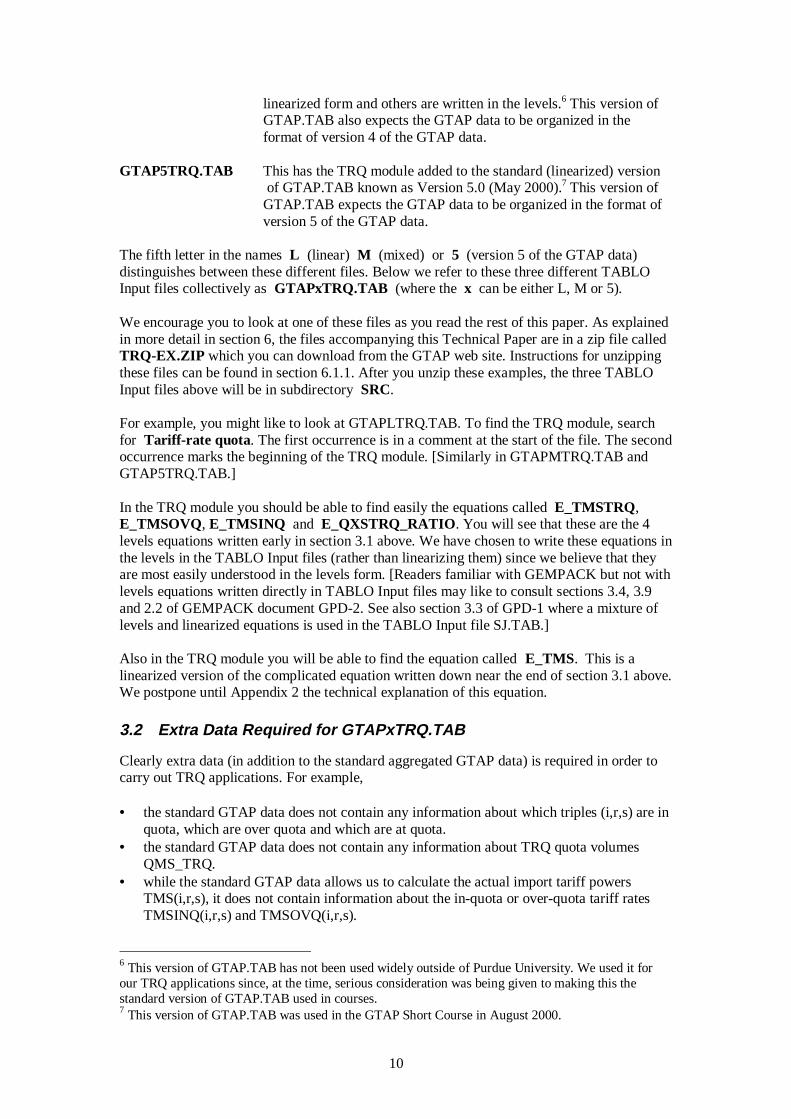
Figure 3 shows a graph of TMSTRQ against QXSTRQ_RATIO. The two 45 degree lineslabelled Line A and Line B have equations

Line A: TMSTRQ + QXSTRQ_RATIO = 2Line B: TMSTRQ + QXSTRQ_RATIO = 1 + TMSTRQOVQ

We have introduced these lines because they assist us in describing the TRQ behavior.

(i) If the current (TMSTRQ,QXSTRQ_RATIO) point is below or on Line A (that is,if TMSTRQ + QXSTRQ_RATIO <= 2) then we want to impose the equationTMSTRQ = 1.

(ii) If the current (TMSTRQ,QXSTRQ_RATIO) point is above or on Line B (that is,if TMSTRQ + QXSTRQ_RATIO >= 1 + TMSTRQOVQ) then we want to impose theequationTMSTRQ = TMSTRQOVQ .

(iii) If the current (TMSTRQ,QXSTRQ_RATIO) point is between Line A and Line B(that is, if TMSTRQ + QXSTRQ_RATIO > 2 and TMSTRQ+QXSTRQ_RATIO < 1 +TMSTRQOVQ)then we want to impose the equationQXS = QMS_TRQ.

This equation can be written as

IF(TMSTRQ + QXSTRQ_RATIO <= 2, TMSTRQ = 1),ELSE IF(TMSTRQ + QXSTRQ_RATIO >= 1 + TMSTRQOVQ, TMSTRQ = TMSTRQOVQ),ELSE IF(TMSTRQ + QXSTRQ_RATIO > 2 and TMSTRQ + QXSTRQ_RATIO < 1+TMSTRQOVQ, QXS = QMS_TRQ).

In code (that is, the TABLO Input files – see section 3.1.1 below), we use the CoefficientTRQPOS to indicate the position of a point in relation to lines A and B. The TRQPOS valuesassigned are shown in Figure 3.3

3 Accurate solutions of the model should be exactly on one of the 3 straight lines shown in Figure 2.[That is, either TMS=TMSINQ, QXS=QMS_TRQ or TMS=TMSOVQ.] However, in the process ofsolving the model, we expect to move at least slightly off these lines. This is why a unique TRQPOSvalue must be assigned to all possible points in Figure 3.

9

A linearized version of the above equation, called E_TMS, is included in the TABLO Inputfiles (see section 3.1.1 below) for solving GTAP with TRQs. We postpone until Appendix 2 adiscussion of this linearized equation.

It is this last equation that causes the problems for GEMPACK whose solution algorithms arenot well suited to handling such non-smooth levels equations. Fortunately it is possible tosolve this equation accurately despite this. The methods (which are described in detail in therest of this paper) are similar to the methods used to implement ordinary import and exportvolume quotas, as documented in GTAP Technical Paper Number 4 (Bach and Pearson,1996). These methods are based on insights provided by Mark Horridge (1993).

Figure 3: The 3 Cases in Equation E_TMS

3.1.1 TRQ TABLO Input Files GTAPxTRQ.TAB

Accompanying this Technical Paper are three different TABLO Input files4 which you canuse to carry out TRQ applications with GTAP. Each has the TRQ equations (as above) in aTRQ module added to a version of GTAP.TAB. These three TABLO Input files are asfollows.

GTAPLTRQ.TAB This has the TRQ module added to the standard (linearized) versionof GTAP.TAB known as Version 4.1 (November 1998).5 Thisversion of GTAP.TAB expects the GTAP data to be organized in theformat of version 4 of the GTAP data.

GTAPMTRQ.TAB This has the TRQ module added to a mixed (linearized/levels)version of GTAP.TAB. We refer to this version of GTAP.TAB as amixed version since some of the usual GTAP equations are written in

4 In GEMPACK, the equations of the model are written down in a so-called TABLO Input file.5 This version of GTAP.TAB was used in the GTAP Short Course in August 1999.

TMSTRQ

QXSTRQ_RATIO

TMSTRQ + QXSTRQ_RATIO = 2

TMSTRQ + QXSTRQ_RATIO =1+TMSTRQOVQTRQPOS=-1

TRQPOS= 0TRQPOS= 1

1

1

BA

10

linearized form and others are written in the levels.6 This version ofGTAP.TAB also expects the GTAP data to be organized in theformat of version 4 of the GTAP data.

GTAP5TRQ.TAB This has the TRQ module added to the standard (linearized) version of GTAP.TAB known as Version 5.0 (May 2000).7 This version ofGTAP.TAB expects the GTAP data to be organized in the format ofversion 5 of the GTAP data.

The fifth letter in the names L (linear) M (mixed) or 5 (version 5 of the GTAP data)distinguishes between these different files. Below we refer to these three different TABLOInput files collectively as GTAPxTRQ.TAB (where the x can be either L, M or 5).

We encourage you to look at one of these files as you read the rest of this paper. As explainedin more detail in section 6, the files accompanying this Technical Paper are in a zip file calledTRQ-EX.ZIP which you can download from the GTAP web site. Instructions for unzippingthese files can be found in section 6.1.1. After you unzip these examples, the three TABLOInput files above will be in subdirectory SRC.

For example, you might like to look at GTAPLTRQ.TAB. To find the TRQ module, searchfor Tariff-rate quota . The first occurrence is in a comment at the start of the file. The secondoccurrence marks the beginning of the TRQ module. [Similarly in GTAPMTRQ.TAB andGTAP5TRQ.TAB.]

In the TRQ module you should be able to find easily the equations called E_TMSTRQ,E_TMSOVQ, E_TMSINQ and E_QXSTRQ_RATIO . You will see that these are the 4levels equations written early in section 3.1 above. We have chosen to write these equations inthe levels in the TABLO Input files (rather than linearizing them) since we believe that theyare most easily understood in the levels form. [Readers familiar with GEMPACK but not withlevels equations written directly in TABLO Input files may like to consult sections 3.4, 3.9and 2.2 of GEMPACK document GPD-2. See also section 3.3 of GPD-1 where a mixture oflevels and linearized equations is used in the TABLO Input file SJ.TAB.]

Also in the TRQ module you will be able to find the equation called E_TMS. This is alinearized version of the complicated equation written down near the end of section 3.1 above.We postpone until Appendix 2 the technical explanation of this equation.

3.2 Extra Data Required for GTAPxTRQ.TAB

Clearly extra data (in addition to the standard aggregated GTAP data) is required in order tocarry out TRQ applications. For example,

• the standard GTAP data does not contain any information about which triples (i,r,s) are inquota, which are over quota and which are at quota.

• the standard GTAP data does not contain any information about TRQ quota volumesQMS_TRQ.

• while the standard GTAP data allows us to calculate the actual import tariff powersTMS(i,r,s), it does not contain information about the in-quota or over-quota tariff ratesTMSINQ(i,r,s) and TMSOVQ(i,r,s).

6 This version of GTAP.TAB has not been used widely outside of Purdue University. We used it forour TRQ applications since, at the time, serious consideration was being given to making this thestandard version of GTAP.TAB used in courses.7 This version of GTAP.TAB was used in the GTAP Short Course in August 2000.

11

Outside estimates of these extra data must be obtained, and care must be taken to ensure thatthese outside estimates are consistent with the rest of the GTAP data you are using.

In section 3.2.1 below we indicate the extra data required for the TRQ module in the TABLOInput files GTAPxTRQ.TAB. In the rest of this section we indicate the sources we used forthe extra data and the steps taken to ensure that these extra data are consistent with the rest ofthe GTAP data we were using.

3.2.1 Extra Data in the TRQ Module in GTAPxTRQ.TAB

It must be possible to obtain a levels solution of the model from the pre-simulation data base.In particular, we need data which will let us infer the pre-simulation values of the in-quotaand over-quota powers of the tariff, and also information from which we can infer the quotavolumes QMS_TRQ. Accordingly, you might expect that the TRQ module inGTAPxTRQ.TAB will require the values of TMSINQ, TMSOVQ and QMS_TRQ for eachtriple (i,r,s).

While we could have required these three arrays, you can see by examining one of theGTAPxTRQ.TAB files that they require three different arrays of extra data, namely

TMSTRQOVQ(i,r,s) The extra power of the tariff levied on over-quota imports [this isin addition to TMSINQ(i,r,s)]

VIWS_TRQ(i,r,s) The value of the quota volume QMS_TRQ of imports at world pricesVIMSINQ_TRQ(i,r,s) The value of the quota volume QMS_TRQ of imports at the world

price plus the in-quota tariff rate

In-quota tariff TMSINQ

The value of TMSINQ can be inferred from the last two of these via

TMSINQ=VIMSINQ_TRQ/VIWS_TRQ.

Over-quota tariff rates

From the usual GTAP data base we can infer the value of the whole actual power of the tariffTMS by dividing VIMS by VIWS. Thus the equations

TMSTRQ = TMS/TMSINQTMSOVQ = TMSINQ * TMSTRQOVQ

allow us to infer the values of TMSTRQ and TMSOVQ.

Quota volumes

We prefer not to read explicit volume data (to avoid the problem of units on our data base).This is why we prefer to hold VIWS_TRQ rather than QMS_TRQ on our TRQ data base.

Firstly note that we can infer the quota ratio QXSTRQ_RATIO from the equation

QXSTRQ_RATIO = VIWS/VIWS_TRQ .

Once we know this quota ratio, we know whether any triple (i,r,s) is in quota (quota ratio < 1),over quota (quota ratio > 1) or at quota (quota ratio = 1). Thus the values of this quota ratioare very useful in working with TRQs.

12

Secondly, we can infer the actual quota volume from the equation

QMS_TRQ = VIWS_TRQ / PCIF

(where PCIF is the levels value of the cif price) if we know the value of PCIF. For this reasonwe have found it convenient to keep track of PCIF in the TRQ module.8 The pre-simulationvalue of PCIF is set equal to one (this amounts to a choice of volume units) and its values areupdated through a simulation via update statements.

Logical File TRQDATA in GTAPxTRQ.TAB

If you look at one of the GTAPxTRQ.TAB files, you will see that the three arrays of extraTRQ data are read from a logical data file called TRQDATA . For example, you will see thatthe TMSTRQOVQ values are read from header “TMS2”.

You will also see, for example, formulas which derive pre-simulation values of TMSINQ,TMSTRQ and TMSOVQ from the values of these extra data and TMS.

Redundancy for over-quota triples

Note that, for a triple (i,r,s) which is over quota, the value of TMSTRQOVQ is redundant.This is because the value of TMSINQ can be inferred from VIWS_TRQ andVIMSINQ_TRQ, the value of TMS can be inferred from the usual GTAP data, we know thatTMSOVQ=TMS (since it is over quota) and hence TMSTRQOVQ can be calculated as

TMSTRQOVQ = TMSOVQ/TMSINQ=TMS/[VIMSINQ_TRQ/VIWS_TRQ].

However, the values of TMSTRQOVQ for triples (i,r,s) which are not over quota cannot beinferred from the rest of the data.

Although this redundancy is an undesirable feature of the data base, we judged the alternativeof storing on the data base just the values of TMSTRQOVQ for triples (i,r,s) which are notover quota to be less desirable (since the set of such triples may change each time a simulationis carried out). Instead when the data base is made, care must be taken to ensure that thepotentially redundant values are consistent with the other data.

3.3 Collecting and Processing Extra TRQ Data – TRQDATA.TAB

As indicated in section 3.2.1 above, the implementation of the TRQ model described hererequires 3 extra arrays of data (over and above the data required for standard GTAP). Theseare the arrays: TMSTRQOVQ(i,r,s), VIWS_TRQ(i,r,s) and VIMSINQ_TRQ(i,r,s) definedabove.

How can you add the extra arrays of data? You will need outside estimates as to which triplesare in quota, which are over quota and which are exactly on quota. You will also look foroutside information about the sizes of TMSINQ, TMSOVQ and QMS_TRQ. If you find datasources for these, they are probably not consistent with the rest of the GTAP data. Forexample, if your outside data tells you TMSINQ and TMSOVQ for a triple which is overquota, the product of TMSINQ and TMSOVQ is probably not equal to TMS inferred by theGTAP data. In such a case, you will need to modify either the outside data or the GTAP datato make them consistent.

8 In GTAPLTRQ.TAB and GTAP5TRQ.TAB, the levels value of PCIF is denoted by PCIF_L.

13

For the applications in this paper, we collected TRQ data from various outside sources (asdescribed below). Then we fed this raw data into a data-manipulation programTRQDATA.TAB whose purpose is to check the data, make it consistent with the usual GTAPdata, and then write out the 3 arrays required. Note that here we took the decision not to alterany of the standard GTAP data but rather to take it as given and to modify the extra TRQ datato be consistent with it. [The alternative of changing the standard GTAP data to be consistentwith the extra TRQ data would be considerably more difficult since the many balancingrequirements in the standard GTAP data would need to be preserved.]

Below we say something about the outside data sources we used, and describe some of thesteps in TRQDATA.TAB.

Inputs into TRQDATA.TAB are the following.

QXSTRQ_RATIO(i,r,s) The ratio of imports over TRQ volume (as defined earlier)TARTMSINQ(i,r,s) Estimates (or target values) of the in-quota tariff TMSINQTARTMSTRQOVQ(i,r,s) Estimates (or target values) of TMSTRQOVQ, the full extra

power of the tariff levied on over-quota imports.

The TARTMSINQ and TARTMSTRQOVQ values are estimates of TMSINQ andTMSTRQOVQ values obtained from outside sources.

The benchmark values for the quota and total imports needed to compute QXSTRQ_RATIOwere assembled from external sources such as country WTO submissions on market accessfor quotas and FAO and UNCTAD for the total value of imports for commodity i for region r.

Both TARTMSINQ and TARTMSOVQ data were collected from external sources includingcountry WTO binding schedules or the UNCTAD tariff data base. A very useful source forthese TRQ tariffs is the Agricultural Market Access Database (AMAD) developed by theEconomic Research Service, United States Department of Agriculture, in collaboration with aconsortium of other agencies9.

3.3.1 Some Steps in TRQDATA.TAB

Here we describe some of the steps we took in TRQDATA.TAB to make the outsideestimates of TRQ data consistent with the standard GTAP data.

For triples (i,r,s) representing commodity i, source region r and destination region s, wedistinguished three cases.

Non-TRQ triples. These are triples for which the data says that imports are in quota. In theapplications in this paper, we were only interested in sugar as a possible TRQ commodity.And we were only interested in TRQs on imports of sugar into USA and EU. Accordingly weforced (in TRQDATA.TAB) all other triples to be non-TRQ triples. We also forced to be non-TRQ triples any triples (i,r,s) for which imports were small in value or for which the TMSvalue in the GTAP data was less than 1.2. For these non-TRQ triples, we overrode anyoutside estimates of QXSTRQ_RATIO and set this ratio to be equal to 0.125 (meaning thatcurrent imports were one-eighth of the volume required to trigger a TRQ tariff). We alsooverrode any outside estimates of TMSTRQOVQ and set this equal to 8. We chose thesevalues of 0.125 and 8 to make it highly unlikely that these triples would ever have importswhich were over the TRQ volume, whatever the changes to the world economy. Note that the

9 The collaborative agencies that contributed to the development of AMAD database include inaddition to ERS/USDA: Agriculture and Agri-Food Canada, EU Commission, DG Agriculture, OECD,UNCTAD, FAO. For access to the database refer to the AMAD home page: www.amad.org

14

TABLO Input files GTAPxTRQ.TAB require values of QXSTRQ_RATIO andTMSTRQOVQ for all triples (i,r,s), even ones for which you never expect a tariff rate quotato be applied.

On quota triples. Here we assumed (potentially overriding the external data) thatTMSINQ=TMSTRQ so that TMSINQ and TMSTRQ are both equal to the square root ofTMS10 (as measured from the standard GTAP data). However, for triples for which TMS inthe GTAP data is less than 1.1, we set TMSTRQ=TMS (and hence TMSINQ=1) to make surethat TMSINQ was never less than 1. [In fact, in our 6x4 data, there were no triples exactly onquota.]

Over quota triples. Here we know that TMSOVQ must equal the TMS shown in the standardGTAP data (since this triple is over quota), and we know from one of the equations in section3.1 that TMSOVQ=TMSINQ*TMSTRQOVQ. But we also have outside estimatesTARTMSINQ of TMSINQ and TARTMSTRQOVQ of TMSTRQOVQ, and it is highly likelythat the product of TARTMSINQ and TARTMSTRQOVQ is not equal to TMS. So we mayneed to modify these outside values. We chose to preserve the ratio between these outsideestimates. That is, we chose to set

TMSINQ/TMSTRQOVQ = TARTMSINQ/TARTMSTRQOVQ.This, plus the known value of TMS from the GTAP data, fixes the values of TMSINQ andTMSTRQOVQ.11 Again this formula could make TMSTRQ less than one. In that case, weoverrode the external data and set TMSTRQ equal to 1.2.

Once the value of TMSTRQ is set for all triples, it is a simple matter to calculate and writeout the values of TMSTRQOVQ, VIWS_TRQ and VIMSINQ_TRQ required forGTAPxTRQ.TAB. [It is easy to calculate them to be consistent with the desiredQXSTRQ_RATIO values and the VIWS values in the standard GTAP data.]

These additional tariff data are read as text files when running the program TRQDATA.TAB.The latter generates the values of: VIWS_TRQ, VIMSINQ_TRQ, and TMSTRQOVQ. Theseoutput arrays from TRQDATA.TAB are all held on a new Header Array file whose logicalname is TRQDATA in both the TABLO files TRQDATA.TAB and GTAPxTRQ.TAB.

This represents Step 1 in Figure 5.

If you collect your own outside data in order to carry out TRQ applications, you will need toreconcile it with the standard GTAP data. You will need to make decisions similar to the oneswe have made (as discussed above). You will probably find a variant of TRQDATA.TABuseful in doing this.

3.3.2 The 4-commodity, 6-region Data Used in the Applications

The TRQ applications in this paper are based on a 4-commodity, 6-region aggregation ofversion 4 of the GTAP data. This aggregation was aimed at modelling the effects of TRQs onsugar. As indicated above, we chose not to modify any of the standard GTAP data set wewere working with, but rather modified the outside estimates of QXSTRQ_RATIO, TMSINQand TMSTRQOVQ to make them consistent with the standard GTAP data.

The commodities in the aggregation used are Sugar, Othag (other agriculture), Mnfcs(manufactures) and Svces (services). The regions are USA, E_U (European Union), ASI(Asia), LAM (Latin America), AFR (Africa) and ROW (Rest of the World). In the TRQ data

10 Recall the equation TMS = TMSINQ * TMSTRQ.11 It is easy to see that TMSTRQ must equal the square root of[TMS*TARTMSTRQOVQ/TARTMSINQ]. This is the formula in TRQDATA.TAB.

15

base we assembled, there are just 9 triples which are over quota, namely imports of sugarfrom ASI, LAM, AFR, ROW into USA and E_U and of sugar from USA into E_U. All othertriples (i,r,s) are in quota. There are no triples in the base data which are exactly on quota.

The files supplied includeDAT6X4.HAR the GTAPDATA filePAR6X4.DAT the GTAPPARM fileSET6X4.HAR the GTAPSETS fileTRQ6X4.HAR the TRQDATA file (which contains the extra TRQ data described above)

3.4 Checks on the Extra Data

The TRQ implementation described here requires TMSOVQ and QMS_TRQ values for everytriple (i,r,s), even for those triples where, in practice, you never expect a tariff rate quota to beapplied.

For triples where no TRQ is in place, and is not likely to be put in place, we recommend

• setting TMSTRQOVQ at a large value (we have used 8 in our additions to the 6x4 data –see section 3.3.1 above), and

• setting QXSTRQ_RATIO equal to a small value (0.125 or 1/8) so that QMS_TRQ equalto 8 times the current import QXS. That is, set VIWS_TRQ equal to 8 times the value ofVIWS shown in the data.

The implementation supplied here will not work unless

TMSTRQOVQ(i,r,s) > 1 for all (i,r,s)1 <= TMS(i,r,s) <= TMSTRQ(i,r,s) in the base data for all (i,r,s).

We recommend that TMSTRQOVQ(i,r,s) is never just a little larger than 1 (say at least 1.2).

It is also vital that the extra data satisfy the levels equations underpinning TRQ. For example,

• if VIWS(i,r,s) > VIWS_TRQ(i,r,s) then TMS(i,r,s) must equal TMSOVQ(i,r,s) since thisis over quota. [Here TMS(i,r,s) is the value implied by VIMS(i,r,s) and VIWS(i,r,s) in thedata.] Also the value of TMSTRQOVQ(i,r,s) in the extra data must be consistent with thevalues of TMSINQ(i,r,s) inferred from the VIWS_TRQ(i,r,s) and VIMSINQ_TRQ(i,r,s)values in the extra data and the value of TMS(i,r,s) inferred from the data.[TMSINQ*TMSTRQOVQ must equal TMS.]

• if VIWS(i,r,s) < VIWS_TRQ(i,r,s) then TMS(i,r,s) must equal TMSINQ(i,r,s) since this isin quota.

• if VIWS(i,r,s) = VIWS_TRQ(i,r,s) then TMSTRQ(i,r,s) must be between 1 andTMSTRQOVQ(i,r,s).

We have built checks such as those above into the various TABLO Input files (including theGTAPxTRQ.TAB files) supplied with this paper.

If you use a TABLO file for ensuring that outside estimates of TRQ data are made consistentwith the base GTAP data (as we do), you should build in checks to ensure that all TRQ levelsequations are satisfied.

16

3.5 Quota Rents

One of the critical issues in analysing the consequence of TRQ liberalization is thedistributional effects of rents between importers and exporters. In our TRQ model, the rest ofthe economy adjusts endogenously to exogenous changes in the split of a quota rent betweenthe exporting region and the importing region. This process requires additional variables andequations.

The variable QUOTA_RENT(i,r,s) is used to denote the value of the total quota rent for agiven bilateral flow (i,r,s) under TRQ. This quota rent corresponds to the shaded areas incases 2 and 3 in Figure 1. The equation determining QUOTA_RENT is:

QUOTA_RENT(i,r,s) = (TMSTRQ(i,r,s) -1) * MIN[(QXS(i,r,s),QMS_TRQ(i,r,s)]

That is: IF QXS(i,r,s) <= QMS_TRQ(i,r,s), thenQUOTA_RENT(i,r,s) = (TMSTRQ(i,r,s) -1) * QXS(i,r,s)

IF QXS(i,r,s) > QMS_TRQ(i,r,s), thenQUOTA_RENT(i,r,s) = (TMSTRQ(i,r,s) -1) * QMS_TRQ(i,r,s)

Note that in the case when imports are below the quota volume, TMSTRQ(i,r,s) is 1 and thequota rents are zero.

3.6 Reallocating Quota Rent Between Importing and Exporting Regions

The variable QRSHARE_X(i,r,s) is used to denote the share of the quota rent associatedwith the triple (i,r,s) that accrues to the exporter. This means that, of the total quota rent, thevalue QRENT_M(i,r,s) allocated to the importing region s is given by the followingequation:

QRENT_M (i,r,s) = [1 – QRSHARE_X (i,r,s)] * QUOTA_RENT(i,r,s)

Likewise, the value QRENT_X(i,r,s) is the quota rent that accrues to the exporting region ris given by the following equation:

QRENT_X (i,r,s) = QRSHARE_X(i,r,s) * QUOTA_RENT(i,r,s)

Any redistribution of quota rents between importers and exporters requires incomeredistribution among the regions consistent with the underlying income/expenditure balanceof the model (as explained below).

In the standard version of the GTAP model, it is assumed that all rents associated with importtariffs accrue to the importing region. This can be seen from the equation namedREGIONALINCOME in the standard GTAP.TAB.12 Since our model allows for quota rentsto be split between importing and exporting regions, a change is needed in the householdincome equation REGIONALINCOME. 12 In the standard GTAP.TAB, the termssum(i,TRAD_COMM, sum(s,REG, {VIMS(i,s,r) * [pms(i,s,r) + qxs(i,s,r)]} - {VIWS(i,s,r) * [pcif(i,s,r) + qxs(i,s,r)]}))on the right-hand side of the REGIONALINCOME equation show this. This is even clearer in themixed linear/levels version of the theory which can be found at the top of the file GTAPMTRQ.TABdistributed with this paper. There the REGIONALINCOME equation is shown in the levels and theterm sum(i,TRAD_COMM, sum(s,REG, VIMS(i,s,r) - VIWS(i,s,r) ))shows that all import tariff revenue accrues to the importing region r.

17

First, the quota portion that accrues to the exporter (QRENT_X(i,r,s)) is subtracted from theimport tariff revenue portion of income in region r as follows:

Sum (i,TRAD_COMM, sum(s,REG, VIMS(i,s,r) - VIWS(i,s,r) - QRENT_X(i,s,r)))

In addition the income equation is augmented by the term TQRENT_X(r) which representsthe sum of quota rents for all TRQ flows captured by region r as an exporter:

TQRENT_X(r) = sum(i,TRAD_COMM, sum{s,REG, QRENT_X(i,r,s)})

3.6.1 Extra Data Required for Rent Reallocation

Our implementation requires QRSHARE_X data for each triple (i,r,s). This data needs to beon a text file (QRSHAR6x4.DAT) and is read from the logical file called QRSHAREX in theTABLO Input files GTAPxTRQ.TAB.

If you are basing your data on a standard GTAP data set (as discussed in section 3.2 above),you should set all these QRSHARE_X values to zero since, as explained above, this is what isassumed in the standard GTAP theory. Then, if you wish to redistribute some of the quotarents to exporters because you think that this more accurately represents reality, you can usethe model to create this modified data, following the procedure outlined in section 3.6.3.

3.6.2 Rent Reallocation Data for the Application

To complement the data files shown in section 3.2.2 above, we have supplied the fileQSHR6X4.DAT which has all the QRSHARE_X values set at zero.

This is not the starting QRSHAREX data file for the applications in section 5 below,however. Rather those applications start from versions of the data in which some quota rentshave already been allocated to exporters (following the procedure described in section 3.6.3).The hands-on details in section 6.9 below will make it clear how you can produce thesemodified data files for yourself.

3.6.3 Creating Data Bases with Quota Rents Redistributed

Suppose that you have collected QRSHARE_X data that shows nonzero shares going to someexporters. You should not simply use this with the other data files you have from a standardGTAP data set (augmented by TRQDATA information as in section 0 above). This is becausethe standard GTAP theory and data assume all import tariffs accrues to importers. Rather youshould use the model to reallocate quota rents as follows.

The idea is to run a simulation that starts from the standard GTAP data, augmented by theTRQDATA and with zero values for all QRSHARE_X values. Then run a simulation withthe standard closure for the TRQ model in which you shock these QRSHARE_X values to thedesired ones.

For example, if you want exporters of sugar from Asia to USA to gain 80 percent of theassociated quota rent, you would give a shock of 0.8 toc_QRSHARE_X(“sugar”,”ASI”,”USA”). This will move the share from zero to the desiredvalue of 0.8. Similarly for other triples.

18

The output of this simulation will be updated GTAPDATA, TRQDATA and QRSHAREX13

data files. These are the files that best represent your collected QRSHARE_X values. Youshould use these (together with the original GTAPSETS and GTAPPARM files) as thestarting point for TRQ applications.

An example of this procedure can be found in the examples discussed in section 6 below. Thepurpose of the example referred to as CASE 0 (see section 6.9.1) is to produce data files inwhich exporters of sugar from 4 regions to USA are allocated 80% of the associated quotarent. The data files produced in CASE 0 are the starting data files for the TRQ applicationsdescribed in section 6.9 below.

3.6.4 Obtaining this QRSHARE_X Data

Although direct data on quota rent shares between importers and exporters are difficult togather, the mechanism by which the TRQ is administered can serve as a guide for allocationrules to use for modelling purposes. For example in the case of first-come first served, onewould expect the quota rents to be shared by both importers and exporters. On the other handif the right to import is given to importers, then presumably all or most of the quota rentsaccrue to the importing country.

Also, exporters may capture most or all of the quota rents if they benefit from beneficialaccess based on existing preferential agreements (for example, the Lome agreement betweenthe EU and ACP countries). In the end, knowledge about the mechanism of TRQadministration as well as possible bilateral or regional trading agreements should informabout the most realistic assumptions of quota rent shares to use for TRQ analysis.

3.6.5 Associated Change to EV_ALT in GTAPxTRQ.TAB

The usual GTAP.TAB files include EV_ALT as an alternative measure of welfare. The valuesof EV and EV_ALT should be equal. A change in the calculation of EV_ALT is requiredwhen there is redistribution of quota rents from importers to exporters. You might like to lookat the equation for EV_ALT in one of the GTAPxTRQ.TAB files to see this change. [Withoutthis change, the values of EV and EV_ALT may not be equal.] We are grateful to MarkusLips for suggesting a workable modification of the EV_ALT equation.

3.7 Tariff Revenues

In TRQ policy analysis, it is useful to report separately changes in tariff revenues associatedwith in-quota imports and out-of-quota imports. In this model, we assume that all importsbelow the quota volume are charged the in-quota tariff (TMSINQ) and all extra imports out-ofthe quota are charged the higher tariffs (TMSOVQ). In other words, we abstract fromfrequent cases when countries may continue to charge only TMSINQ for out-of quotaimports.

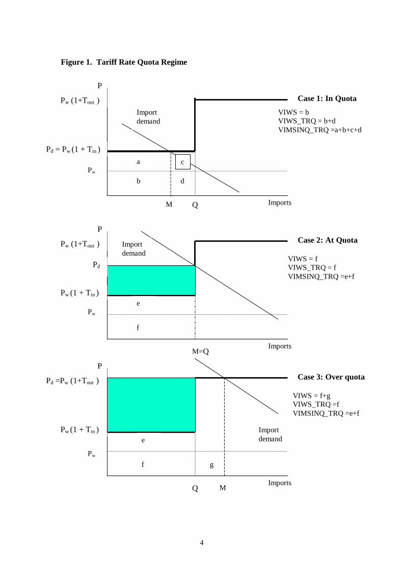
Reporting tariff revenues requires additional variables and equations. The first equationcalculates the total tariff revenue variable TTRF_REV(.):

TTRF_REV(i,r,s)= VIMS(i,r,s) - VIWS(i,r,s) - QRENT(i,r,s)

Next is the equation that defines tariff revenue associated with in-quota imports:

INTRFREV(i,r,s) =

13 Of course, the values in the updated QRSHAREX file will just be your desired QRSHARE_X valuessince you started from all values zero and gave these desired values as shocks.

19

(TMSINQ(i,r,s) -1) * MIN[(VIWS(i,r,s),VIWS_TRQ(i,r,s)]

That is: IF VIWS(i,r,s) <= VIWS_TRQ(i,r,s), thenINTRFREV(i,r,s) = (TMSINQ(i,r,s) -1) * VIWS(i,r,s)

IF VIWS(i,r,s) > VIWS_TRQ(i,r,s), thenINTRFREV(i,r,s) = (TMSINQ(i,r,s) -1) * VIWS_TRQ(i,r,s);

From the two equations above, the tariff revenue portion from the out-of quota imports isderived as:

OVTRFREV(i,r,s)= TTRF_REV(i,r,s) – INTRFREV(i,r,s)

These revenue components are illustrated in Figure 4 below.

Figure 4. Quota Rent and Tariff Revenue

over

-quo

ta ta

riff

reve

nue

(OV

TR

FR

EV

)

PCIF

PMS

QMS_TRQ

quota rent(QUOTA_RENT)

in-quota tariff revenue(INTRFREV)

P

Q

Importdemand

20

4 GEMPACK Procedures for One Simulation

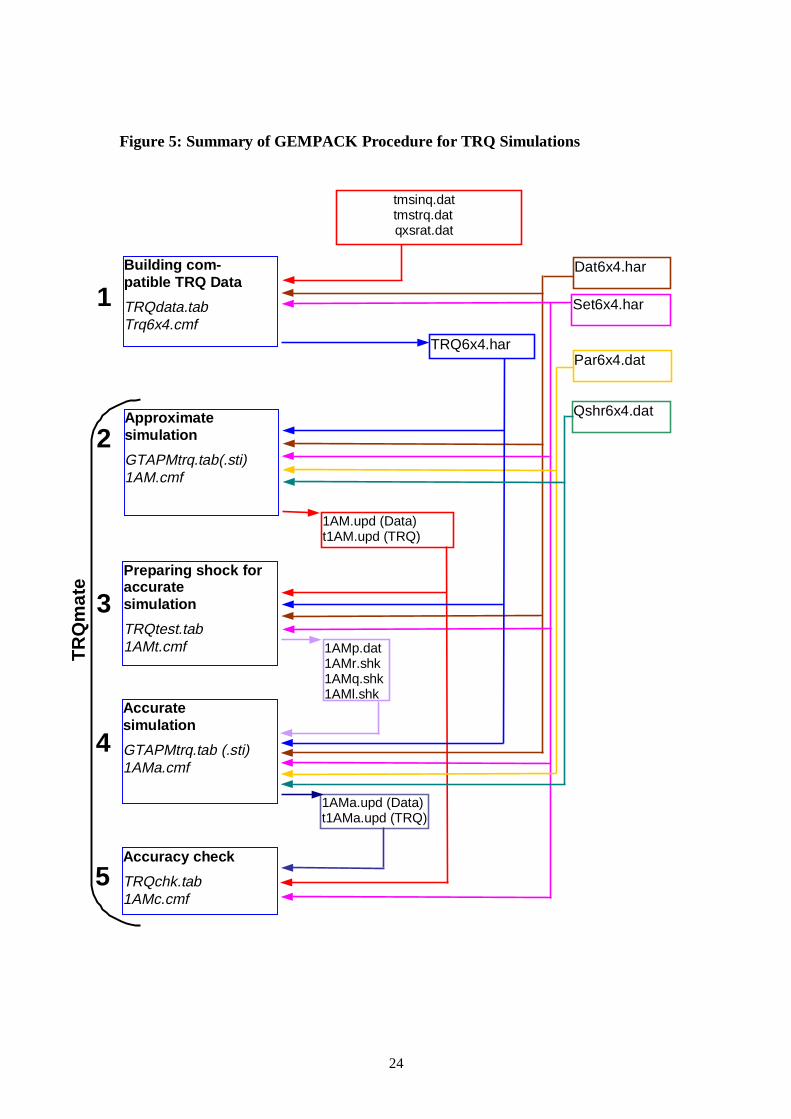
As with quotas [see Bach and Pearson (1996)], a complete TRQ scenario consist of asequence of calculations carried out consecutively. Steps 2-5 in Figure 5 provide a summaryof the various calculations needed to carry a complete TRQ simulation.

Note that, besides the TABLO Input file for the model (one of the GTAPxTRQ.TAB files),two other data-manipulation TABLO Input files

TRQTEST.TAB and TRQCHK.TAB

are used in this sequence of calculations.

4.1 Overview of the Procedures

As you can see from Figure 5,

• an approximate version of the simulation is first carried out (Step 2).• then TRQTEST is run (Step 3).• then an accurate version of the simulation is run (Step 4).• finally TRQCHK is run (Step 5).

The purpose of these different calculations is explained below.

4.1.1 Purpose of the Approximate Simulation

Before doing an accurate simulation it is necessary to carry out an approximate simulationwhich is always done as a single multi-step Euler calculation. The approximate version of thesimulation is run solely to find out the post-simulation TRQ status of each triple (i,r,s). Thatis, to find out if this triple will be in quota, over quota or exactly on quota in the post-simulation world. Once this is known, there is standard machinery (as outlined below) to setup an accurate version of the simulation which forces the model to these TRQ positions and inwhich the usual GEMPACK solution extrapolation procedure can be used to producearbitrarily accurate simulation results.

4.1.2 Sequence of Calculations

• First run the approximate version of the simulation.• After this, a calculation must be made (using TRQTEST.TAB) to find out, for each triple

(i,r,s), which part of the TMSTRQ/QXS curve (as shown in Figure 3 above) the updateddata is nearest to, and what shocks are required to move from the pre-simulation data tothis point. [This calculation uses the updated data after the approximate simulation.]

• This information is fed into the accurate version of the simulation and used to specify analternative closure and additional shocks for the accurate simulation. This alternativeclosure and extra shocks are chosen to guarantee that, for each triple (i,r,s), theTMSTRQ/QXS position in the post-simulation data after the accurate simulation is onexactly the same part of the curve as was reached after the approximate simulation. [Partof the closure and shocks specification for this run relies on outputs from the aboveTRQTEST run.]

• Finally, you must run TRQCHK to check that, for each triple (i,r,s), the TRQ status afterthe accurate simulation is the same as that after the approximate simulation. That is checkthat the TMSTRQ/QXS position in the updated data is very close to the TMSTRQ/QXS

21

graph (consisting of two horizontal lines and one vertical straight line). You must alsoinspect the Extrapolation Accuracy Summary in the LOG file of this run to check that thisaccurate simulation converged satisfactorily. If TRQCHK indicates that the TRQ statusfor any triple is different from that expected, you must start all over, this time taking moreEuler steps in the approximate simulation to try to get the post-simulation TRQ statusmore accurately. If the accurate simulation did not converge sufficiently well, you shouldincrease the number of steps used (or, in some cases, switch back to Euler’s method ifGragg’s method seems not to be working well in this case). [The TRQCHK run accessesthe post-simulation data after both the approximate and accurate simulations.]

4.2 The Command File for the Accurate Simulation

This differs from that for the approximate simulation in the solution method andclosure/shocks sections.

4.2.1 Solution Method

For the approximate version you must use Euler’s method (never Gragg) and you should seesomething like (the number of steps may be different):

Method = euler ;Steps = 40 ;

For the accurate simulation, always extrapolate from 3 separate multi-step calculations, anduse Gragg’s method (unless it seems not to work ok, in which case use Euler’s method). Forexample, you might use:

Method = gragg ;Steps = 6 8 10 ;

4.2.2 Closure/Shocks section of Command file for Accurate Simulation

You will need the following additional statements to modify the closure and shocks from theapproximate version.

! Closure and shock changes for accurate versionEndogenous tms_slack ;statements to shock variable with none exogenous are ok = yes ;

Exogenous p_TMSTRQ = negative value on file <TRQPOSVAL> ;Exogenous p_QXSTRQ_RATIO = zero value on file <TRQPOSVAL> ;Exogenous c_TMSTRQBELOVQ = positive value on file <TRQPOSVAL> ;

Shock p_TMSTRQ = select from file <TMSTRQ_SHK> ;Shock p_QXSTRQ_RATIO = select from file <QXSRAT_SHK> ;Shock c_TMSTRQBELOVQ = select from file <TRQBLOVQ_SHK> ;

The TRQTEST job outputs 4 important files. These have logical names TRQPOSVAL,TMSTRQ_SHK, TRQBLOVQ_SHK and QXSRAT_SHK respectively. The above lines usethese logical names (for example <TRQPOSVAL>) but of course the Command file shouldcontain the actual file names (rather than the logical ones).

22

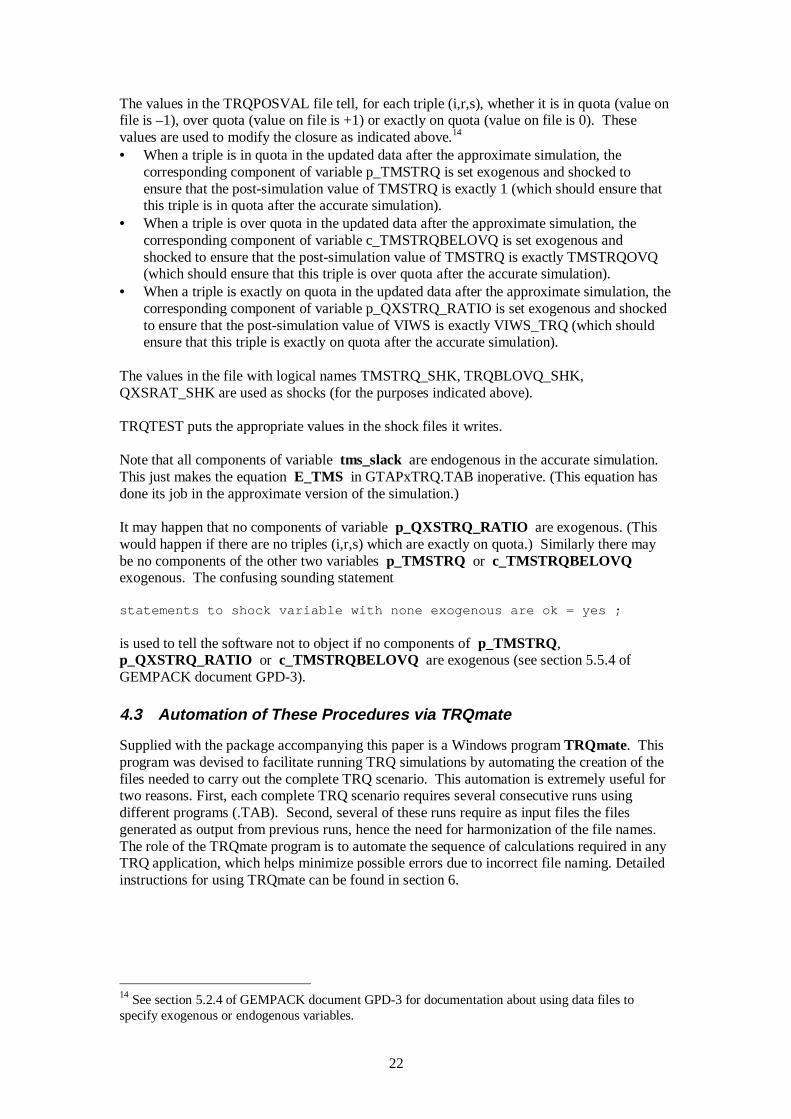
The values in the TRQPOSVAL file tell, for each triple (i,r,s), whether it is in quota (value onfile is –1), over quota (value on file is +1) or exactly on quota (value on file is 0). Thesevalues are used to modify the closure as indicated above.14

• When a triple is in quota in the updated data after the approximate simulation, thecorresponding component of variable p_TMSTRQ is set exogenous and shocked toensure that the post-simulation value of TMSTRQ is exactly 1 (which should ensure thatthis triple is in quota after the accurate simulation).

• When a triple is over quota in the updated data after the approximate simulation, thecorresponding component of variable c_TMSTRQBELOVQ is set exogenous andshocked to ensure that the post-simulation value of TMSTRQ is exactly TMSTRQOVQ(which should ensure that this triple is over quota after the accurate simulation).

• When a triple is exactly on quota in the updated data after the approximate simulation, thecorresponding component of variable p_QXSTRQ_RATIO is set exogenous and shockedto ensure that the post-simulation value of VIWS is exactly VIWS_TRQ (which shouldensure that this triple is exactly on quota after the accurate simulation).

The values in the file with logical names TMSTRQ_SHK, TRQBLOVQ_SHK,QXSRAT_SHK are used as shocks (for the purposes indicated above).

TRQTEST puts the appropriate values in the shock files it writes.

Note that all components of variable tms_slack are endogenous in the accurate simulation.This just makes the equation E_TMS in GTAPxTRQ.TAB inoperative. (This equation hasdone its job in the approximate version of the simulation.)

It may happen that no components of variable p_QXSTRQ_RATIO are exogenous. (Thiswould happen if there are no triples (i,r,s) which are exactly on quota.) Similarly there maybe no components of the other two variables p_TMSTRQ or c_TMSTRQBELOVQexogenous. The confusing sounding statement

statements to shock variable with none exogenous are ok = yes ;

is used to tell the software not to object if no components of p_TMSTRQ,p_QXSTRQ_RATIO or c_TMSTRQBELOVQ are exogenous (see section 5.5.4 ofGEMPACK document GPD-3).

4.3 Automation of These Procedures via TRQmate

Supplied with the package accompanying this paper is a Windows program TRQmate. Thisprogram was devised to facilitate running TRQ simulations by automating the creation of thefiles needed to carry out the complete TRQ scenario. This automation is extremely useful fortwo reasons. First, each complete TRQ scenario requires several consecutive runs usingdifferent programs (.TAB). Second, several of these runs require as input files the filesgenerated as output from previous runs, hence the need for harmonization of the file names.The role of the TRQmate program is to automate the sequence of calculations required in anyTRQ application, which helps minimize possible errors due to incorrect file naming. Detailedinstructions for using TRQmate can be found in section 6.

14 See section 5.2.4 of GEMPACK document GPD-3 for documentation about using data files tospecify exogenous or endogenous variables.

23

4.4 Optional Use of TRQTMS.TAB During a TRQmate Run

There is yet another data-manipulation TABLO Input file supplied to assist with TRQapplications. This is the file TRQTMS.TAB. As you can see by looking at TRQTMS.TAB,the purpose of running TRQTMS is to calculate and report the values of various TRQ-relatedquantities, including

TMSINQ, TMSTRQOVQ, TMSOVQ, TMS, TMSTRQ and QXSTRQ_RATIO.

When you use TRQmate to carry out a TRQ application, you can choose (via the Optionsmenu in TRQmate) to run TRQTMS after both the approximate and accurate simulations (thatis, after Steps 3 and 5 in Figure 5). We have found that looking at some of these values (asoutput by TRQTMS) helps to check the TRQ status of various of the triples (i,r,s), particularlythose whose status changes between the pre-simulation data and the post-simulation data.

Of course, TRQTMS can be used to report these different values for any GTAP data setaugmented by the extra TRQ data (the 3 arrays shown in section 3.2.1). So also TRQTMS canbe run to report the values of the quantities above as found in the pre-simulation data (thoughthis is not an option in TRQmate – you must run it yourself if you want to see thisinformation).

4.5 The Different TABLO Input Files Supplied

You have now been introduced (at least briefly) to the different TABLO Input files suppliedin the software accompanying this paper. These are

GTAPxTRQ.TAB (where “x” is either L, M or 5). See section 3.1.1 . These are used to solvethe model.TRQTEST.TAB and TRQCHK.TAB (see section 4.1.2).TRQTMS.TAB (see section 4.4).TRQDATA.TAB (see section 3.3).

You will learn more about these in section 6.

24

Figure 5: Summary of GEMPACK Procedure for TRQ Simulations

Building com-patible TRQ Data

TRQdata.tabTrq6x4.cmf

Approximatesimulation

GTAPMtrq.tab(.sti)1AM.cmf

Accuratesimulation

GTAPMtrq.tab (.sti)1AMa.cmf

Preparing shock foraccuratesimulation

TRQtest.tab1AMt.cmf

Accuracy check

TRQchk.tab1AMc.cmf

Dat6x4.har

Par6x4.dat

Set6x4.har

1AMp.dat1AMr.shk1AMq.shk1AMl.shk

1AMa.upd (Data)t1AMa.upd (TRQ)

1AM.upd (Data)t1AM.upd (TRQ)

tmsinq.dat tmstrq.dat qxsrat.dat

TRQ6x4.har

5

4

3

2

1

TR

Qm

ate

Qshr6x4.dat

25

5 Policy Application: Partial Liberalization of Sugar TRQ

In this section we illustrate the implementation of the GTAP/TRQ model by quantifying thewelfare and trade effects of U.S. liberalization of its TRQ policy regime for sugar. We usethe 6x4 GTAP aggregation as described in this paper to keep the analysis manageable. In thisapplication we focus on U.S. sugar policy program and simulate alternative scenarios forexpanding TRQs and reducing out-of quota tariffs.

The U.S. maintains a TRQ regime for sugar imports by allocating bilateral quotas to exportingcountries on the basis of their historical market shares. The OECD Secretariat estimates the advalorem equivalent of the out-of-quota tariffs of sugar imported into the U.S. at 129 percent(OECD, 1997). The sugar TRQ regime benefits not only domestic producers (at the expenseof consumers) but also the exporting countries that hold export quota rights in the form ofimplicit subsidy to selected exporters. For example Taiwan, has tariff quota rights for theexport of about 24,000 short tons of sugar to the U.S. (Skully, 1999). While Taiwan alwaysfills its quota (its only sugar export), its domestic production doesn't satisfy its domesticdemand resulting in sugar imports from Thailand and Australia to cover the difference,including the 24,000 tons to cover the domestic production exported to the United States.Similarly the Philippines, another major quota holder of sugar exports to the U.S., hasrecently been unable to cover its domestic needs from domestic production: in fact it has aTRQ to limit sugar imports. If the U.S. liberalizes its sugar TRQ, these countries may lose ifcontraction in quota rents outweighs any revenue increases from expanded trade.

In this section we consider a simple set of counterfactual simulations of TRQ sugarliberalization by the U.S. to illustrate the workings of the model.15 We use a 4-sector 6-regionaggregation. The sectors are: sugar, other agriculture, manufacturing and services. Our focusis on the sugar sector. The regions are: U.S., EU, Asia, Latin America, Africa and Rest ofWorld.

We consider three simple experiments in which only the U.S. liberalizes its sugar TRQ (withrespect to all other regions in the model). The three experiments are:

1) cut in over-quota ad valorem tariff by 33 percent,16

2) expansion of sugar quota by 20 percent, and3) combination of both.

(These correspond to APP1, APP2 and APP3 in the associated files.) All 3 applications startfrom a data base in which 80% of the quota rents accrue to the exporting regions (and only20% to the U.S.).17

Results on trade volume, quota rents, and welfare changes for these 3 applications aresummarized in Table 1.18

15 See Elbehri et al. (1999) for a more complete policy analysis of sugar TRQ liberalization in amultilateral context using the modelling framework outlined in the present paper.16 The actual shocks for this experiment are shocks to the power of the over-quota tariff TMSOVQ.The pre-simulation ad valorem rates for sugar imports into USA are approximately 264.3% for importsfrom EU and 63.8% from the other 4 regions. These are reduced to approximately 156.2% and 42.6%in this application. These correspond to reductions in the power of the over-quota tariff TMSOVQ byapproximately 24.2 percent and 13.0 percent respectively.17 These are the data bases produced by carrying out CASE 0 – see section 6.9.1 below.18 In Table 1, the numbers in the “Welfare” column are the EV results from the model. The numbers inthe “Sugar exports %” column are the qxw results from the model. The numbers in the “Sugar exports

26

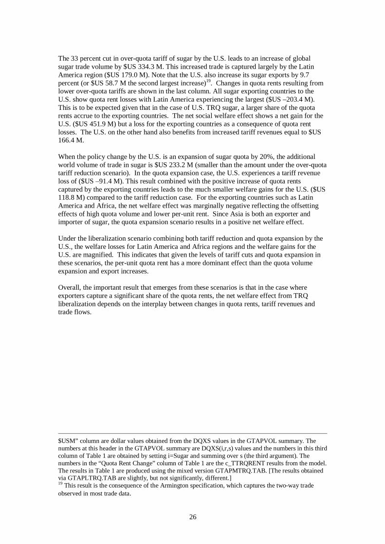
The 33 percent cut in over-quota tariff of sugar by the U.S. leads to an increase of globalsugar trade volume by $US 334.3 M. This increased trade is captured largely by the LatinAmerica region ($US 179.0 M). Note that the U.S. also increase its sugar exports by 9.7percent (or $US 58.7 M the second largest increase)19. Changes in quota rents resulting fromlower over-quota tariffs are shown in the last column. All sugar exporting countries to theU.S. show quota rent losses with Latin America experiencing the largest ($US –203.4 M).This is to be expected given that in the case of U.S. TRQ sugar, a larger share of the quotarents accrue to the exporting countries. The net social welfare effect shows a net gain for theU.S. ($US 451.9 M) but a loss for the exporting countries as a consequence of quota rentlosses. The U.S. on the other hand also benefits from increased tariff revenues equal to $US166.4 M.

When the policy change by the U.S. is an expansion of sugar quota by 20%, the additionalworld volume of trade in sugar is $US 233.2 M (smaller than the amount under the over-quotatariff reduction scenario). In the quota expansion case, the U.S. experiences a tariff revenueloss of ($US –91.4 M). This result combined with the positive increase of quota rentscaptured by the exporting countries leads to the much smaller welfare gains for the U.S. ($US118.8 M) compared to the tariff reduction case. For the exporting countries such as LatinAmerica and Africa, the net welfare effect was marginally negative reflecting the offsettingeffects of high quota volume and lower per-unit rent. Since Asia is both an exporter andimporter of sugar, the quota expansion scenario results in a positive net welfare effect.

Under the liberalization scenario combining both tariff reduction and quota expansion by theU.S., the welfare losses for Latin America and Africa regions and the welfare gains for theU.S. are magnified. This indicates that given the levels of tariff cuts and quota expansion inthese scenarios, the per-unit quota rent has a more dominant effect than the quota volumeexpansion and export increases.

Overall, the important result that emerges from these scenarios is that in the case whereexporters capture a significant share of the quota rents, the net welfare effect from TRQliberalization depends on the interplay between changes in quota rents, tariff revenues andtrade flows.

$USM” column are dollar values obtained from the DQXS values in the GTAPVOL summary. Thenumbers at this header in the GTAPVOL summary are DQXS(i,r,s) values and the numbers in this thirdcolumn of Table 1 are obtained by setting i=Sugar and summing over s (the third argument). Thenumbers in the “Quota Rent Change” column of Table 1 are the c_TTRQRENT results from the model.The results in Table 1 are produced using the mixed version GTAPMTRQ.TAB. [The results obtainedvia GTAPLTRQ.TAB are slightly, but not significantly, different.]19 This result is the consequence of the Armington specification, which captures the two-way tradeobserved in most trade data.

27

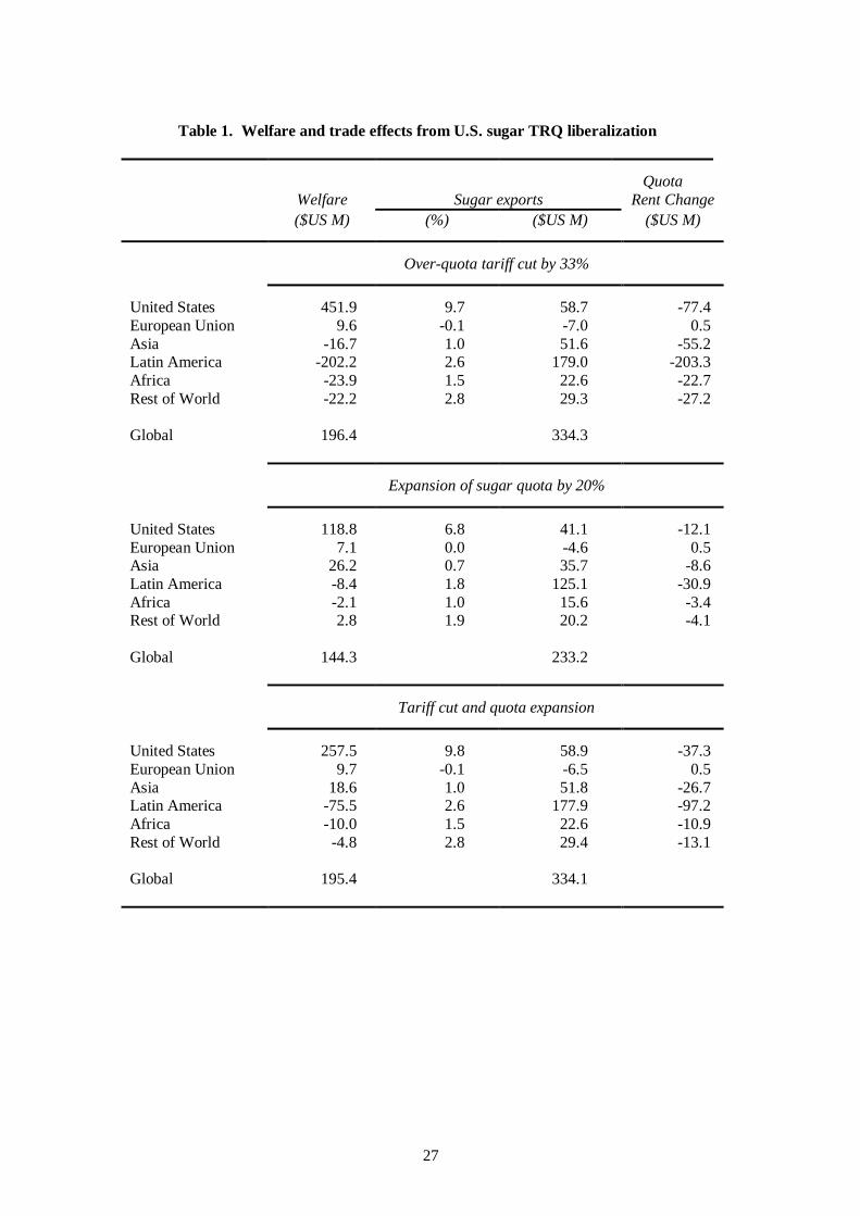
Table 1. Welfare and trade effects from U.S. sugar TRQ liberalization

QuotaWelfare Sugar exports Rent Change($US M) (%) ($US M) ($US M)

Over-quota tariff cut by 33%

United States 451.9 9.7 58.7 -77.4European Union 9.6 -0.1 -7.0 0.5Asia -16.7 1.0 51.6 -55.2Latin America -202.2 2.6 179.0 -203.3Africa -23.9 1.5 22.6 -22.7Rest of World -22.2 2.8 29.3 -27.2

Global 196.4 334.3

Expansion of sugar quota by 20%

United States 118.8 6.8 41.1 -12.1European Union 7.1 0.0 -4.6 0.5Asia 26.2 0.7 35.7 -8.6Latin America -8.4 1.8 125.1 -30.9Africa -2.1 1.0 15.6 -3.4Rest of World 2.8 1.9 20.2 -4.1

Global 144.3 233.2

Tariff cut and quota expansion

United States 257.5 9.8 58.9 -37.3European Union 9.7 -0.1 -6.5 0.5Asia 18.6 1.0 51.8 -26.7Latin America -75.5 2.6 177.9 -97.2Africa -10.0 1.5 22.6 -10.9Rest of World -4.8 2.8 29.4 -13.1

Global 195.4 334.1

28

6 Examples Supplied

Accompanying this paper are several example applications using the 4-commodity 6-regiondata base. The relevant files are available in a ZIP file TRQ-EX.ZIP which can bedownloaded from the web.

Included in TRQ-EX.ZIP are the various TABLO Input files, namely those in section 4.5above.

Also included are the base data files20

GTAPDATA dat6x4.har or dat6x4v5.harGTAPSETS set6x4.har or set6x4v5.harGTAPPARM par6x4.dat or par6x4v5.harTRQDATA trq6x4.har or trq6x4v5.harQSHAREX qshr6x4.dat

There are two groups of applications,

• some introductory examples designed to teach you about using this version of GTAP,• some more serious applications related to liberalization of TRQs relating to sugar. [These

are the applications whose results are reported in section 5].

To carry out the examples and applications supplied on your own computer, you will need aversion of Release 6.0 or later of GEMPACK installed.21

6.1 Getting Started

Much of the testing of the examples here needs to be done in a DOS box.

6.1.1 Directory Structure for the Examples

We have followed Robert McDougall’s preferred directory structure in the ZIP file whichcontains these examples. You should place the ZIP file TRQ-EX.ZIP in a new directory(perhaps call it C:\GTAPTRQ). Then issue the command

pkunzip -d trq-ex

This will unzip the relevant files. The main input files (including the TABLO Input files) gointo a subdirectory called SRC (source files). The original GTAP data files for the 6x4aggregation are placed in a subdirectory called IN (input files). There is also a subdirectorycalled WRK (working files) to hold various output files.

After you unzip the files, look at the file READ-TRQ.ME to see if there are any updates orcorrections to the information in this paper.

6.1.2 Processing the TABLO Input Files

There are several TABLO Input files, as described in section 4.5 above.22

20 Those with “v5” in their names are for use with GTAP5TRQ.TAB while the others are for use withGTAPLTRQ.TAB and GTAPMTRQ.TAB.21 Either a Source-code or an Executable-image version can be used.

29

TABLO must be run to process each of these TABLO Input files. To do this, go into the mainTRQ directory (C:\GTAPTRQ).

• If you have a Source-code version of GEMPACK, issue the command

tabfiles

This will run the DOS batch job tabfiles.bat which should produce executable images ofthe TABLO-generated programs.

• If you have an Executable-image version of GEMPACK, issue the command

tabfilgs

This will run the DOS batch job tabfilgs.bat which should produce output for GEMSIMfor each of the TABLO Input files in this package.

In each case the output will go in subdirectory WRK .

6.1.3 Making the 6x4 TRQ Data

As we have explained in section 3.3, the TABLO Input file TRQDATA.TAB containsinstructions for reading estimates of TMSINQ, TMSTRQOVQ and QXSTRQ_RATIO forall triples (i,r,s). These estimates have been obtained from data sources outside the usualGTAP data (see section 3.3).

• The estimates of TMSINQ (called TARTMSINQ in TRQDATA.TAB) are read from filein\tmsinq.dat (which corresponds to the logical file TMSINQDAT in TRQDATA.TAB).

• The estimates of TMSTRQOVQ (called TARTMSTRQOVQ in TRQDATA.TAB) areread from file in\tmstrq.dat (which corresponds to the logical file TMSTRQOVQDAT inTRQDATA.TAB).

• The estimates of QXSTRQ_RATIO (called the same name in TRQDATA.TAB) are readfrom file in\qxsrat.dat (which corresponds to the logical file TRQIMPRAT inTRQDATA.TAB).

The job of TRQDATA.TAB is to read these TRQ estimates, make them compatible with theGTAP data in the file in\dat6x4.har and then write them out to the file wrk\trq6x4.har .23

You should look into TRQDATA.TAB to see how this is done. In particular, look towardsthe end of the file to see the checks, which ensure that this extra TRQ data satisfies the levelsequations governing TRQ behavior. These are the checks described earlier in section 3.4.

To run TRQDATA.TAB to produce wrk\trq6x4.har and wrk\trq6x4v5.har, change directoryinto the main TRQ directory (C:\GTAPTRQ) and issue the command

trq6x4 (if you have a Source-code version of GEMPACK)trq6x4gs (if you have an Executable-image version of GEMPACK)

22 Also supplied are files for GTAPVIEW, GTAPVOL and DECOMP – see section 6.11 below.23 These are the file names for our version 4 data files. The version 5 data files are in\dat6x4v5.har (theGTAPDATA file) and wrk\trq6x4v5.har (the output from running TRQDATA.TAB).

30

This will run the DOS batch job trq6x4.bat or trq6x4gs.bat which should producewrk\trq6x4.har (this is based on the version 4 GTAP data) and wrk\trq6x4v5.har (this isbased on the version 5 GTAP data).24

It is a good idea to look at the 6x4 data to see, for example, which triples (i,r,s) are over quota.You can do that by viewing trq6x4.har or trq6x4v5.har, using VIEWHAR. To see whichtriples (i,r,s) are over quota, look at the QXSTRQ_RATIO values via the header QRAT. Youshould see that the only triples which are over quota are those for imports of sugar fromregions ASI (Asia), LAM (Latin America), AFR (Africa), ROW (Rest of World) into each ofUSA and E_U and also imports of sugar from USA into E_U. [These are the triples for whichQXSTRQ_RATIO(i,r,s)>1.] For these triples, look to see the values of TMSINQ,TMSTRQOVQ, TMS and TMSTRQ. [Look in TRQDATA.TAB to see to which headersthese values have been written.] Check, for example, that TMS=TMSINQ*TMSTRQ.

You are now ready to start the example simulations and applications.

6.2 Standard Closures

There are two standard closures used in the examples and applications described below. Thestatements to set them up can be found in the files TRQM1.CLS , TRQM2.CLS,TRQL1.CLS , TRQL2.CLS, V5TRQL1.CLS and V5TRQL2.CLS which you can find inyour SRC subdirectory. The difference between these is that, in the first closure (TRQM1,TRQL1 and V5TRQL1), TMSINQ and TMSTRQOVQ are exogenous (and TMSOVQ adjustsendogenously) while in the second closure (TRQM2, TRQL2 and V5TRQL2), TMSINQ andTMSOVQ are exogenous (and TMSTRQOVQ adjusts endogenously).25

The second standard closure TRQM2.CLS, TRQL2.CLS or V5TRQL2.CLS is selected whenwe need to shock the over-quota tariffs (shock to p_TMSOVQ) without changing the in-quotatariffs (TMSINQ). The following table summarizes the two closure options:

Exogenous EndogenousTRQM1.CLS p_tmsinq, p_tmstrqovq p_tmsovqTRQM2.CLS p_tmsinq, p_tmsovq p_tmstrqovq

These standard closures are used for the approximate simulation. As noted in section 4.2.2,slightly different closures are used for the accurate simulation.

6.3 Introductory Examples

These examples all relate to shocks applied to one of the TRQ triples, namely imports ofsugar from Africa into USA. In the pre-simulation data, such imports are over quota. Indeed,TMSTRQOVQ=1.88, TMS=TMSOVQ=1.64 (import tariff), TMSINQ=0.87 (import subsidyfor in-quota imports), VIWS=122.7 and VIWS_TRQ=116.126 which means thatQXSTRQ_RATIO=1.057 so that import volumes are 5.7 percent above the quota volume.

24 The output files trq6x4.har or trq6x4v5.har contain more than the three arrays which are used asinput to GTAPxTRQ.TAB. For example, they contain the implied QXSTRQ_RATIO values (as youwill see in the next paragraph of the main text). These extra values are written because we have found ituseful to look at them in some cases.25 Closures TRQL1,TRQL2 are for use with GTAPLTRQ.TAB, closures TRQM1,TRQM2 are for usewith GTAPMTRQ.TAB while closures V5TRQL1,V5TQL2 are for use with GTAP5TRQ.TAB.26 These are the VIWS and VIWS_TRQ figures from the version 4 data. For the version 5 data (seein\dat6x4v5.har and wrk\trq6x4v5.har), VIWS = 107.7 and VIWS_TRQ = 101.9.

31

There are several different simulations. We describe them all here briefly. Then, in section 6.4below, we give detailed hands-on instructions which you can follow to carry out theseexamples for yourself.

Use the first standard closure (TRQM1.CLS, TRQL1.CLS or V5TRQL1.CLS – see section6.2 above) in the first 3 lots of examples but use the second standard closure (TRQM2.CLS,TRQL2.CLS or V5TRQL2.CLS) for example 4.

1. Simulations increasing TMSINQ, holding TMSTRQOVQ and QMS_TRQ fixed. SinceTMSTRQOVQ is held fixed, an increase in TMSINQ also causes the same percentageincrease in TMSOVQ. Clearly an increase in TMSINQ should reduce imports. Eventuallyimports should reduce to be exactly on quota. A sufficiently large increase in TMSINQshould reduce imports sufficiently far that they become in quota. It turns out that a 20%increase in TMSINQ reduced imports to be exactly on quota while a 100% increase inTMSINQ leaves imports in quota. These are called CASES 1A and 1B, respectively inthe associated Example files.

2. Simulations increasing QMS_TRQ, holding TMSINQ and TMSTRQOVQ fixed. This atrade liberalization. At first sight it seems that any increase in QMS_TRQ should increaseimports. However a small increase (of less than 5.7%) will leave QMS_TRQ below thecurrent volume of imports and this will have no effect on the volume of imports (or onanything else in the model except for the value of quota rents). This is because importersare prepared to pay the full TMSOVQ tariff for a base period volume of imports which ishigher than the increased QMS_TRQ. Larger increases in QMS_TRQ (more than 5.7%)will lead to increases in imports of sugar from Africa into USA. It turns out that a 20%increase in QMS_TRQ leaves imports exactly on the new quota volume. You wouldexpect a very large increase in QMS_TRQ to leave imports within the new quota volume.Indeed, it seems that a 10 fold increase in QMS_TRQ (that is, 1000 per cent increase)does this. The Example files have two cases, CASE 2A (2% increase in QMS_TRQ)and CASE 2B (20% increase in QMS_TRQ).27

3. A simulation decreasing QMS_TRQ. At first sight, you might expect this to decreaseimports since a decrease in QMS_TRQ is the opposite to a liberalization. In fact adecrease has no effect at all (since the imports are already higher than the existing quota).No volumes or other prices change. The only change is the value of quota rents. This isCASE 3.

4. A simulation increasing TMSOVQ, holding TMSINQ and QMS_TRQ fixed. Anyincrease in TMSOVQ should reduce imports (since the imports are over quota and sosuffer from the increased TMS immediately). It turns out that an increase of 20% inTMSOVQ reduces imports to be exactly on quota. However, even a very large increase inTMSOVQ can not reduce imports to in quota. This is because TMSOVQ has no effect onimports once the import volume is no longer over quota. This is CASE 4.

You can see that each of the simulations above is sufficiently simple that we have a very goodqualitative idea as to what should happen. Carrying out such simulations is a very importantpart of testing any new behavior in a model. When we were developing the TRQ code, thesimulations described above showed up several errors and suboptimalities.

27 We do not include CASE 2C (1000% increase in QMS_TRQ) since we found it difficult to get thisexample to converge due to the very large shock.

32

6.3.1 Reversing these Simulations

Each of the simulations above can be reversed. That is, the opposite shock can be applied tothe post-simulation data. When this is done, the percentage-change results of this reversalsimulation should be the exact opposite of the results of the original simulation. Also the post-simulation (that is, updated) data base after the reversal simulation should be identical to theoriginal data base (up to machine accuracy). These reversal simulations are thus alsoimportant checks of our modelling of TRQs (and they also helped us to identify errors).

Consider the first example simulation (CASE 1A) in which TMSINQ is increased by 20 percent. The simulation results show that imports of sugar from Africa into USA decrease involume by –5.39262 percent.28 What should happen in the reversal simulation? Firstly, theshock in the reversal simulation is not –20% but rather –16.66667%. [This is because if youincrease from 100 by 20% you get to 120. To reverse this, you need to reduce from 120 to100. The corresponding percentage change is –20/120*100=-16.66667.] Similarly the reversalof -5.39262 is 100*(5.39262/94.60738)=5.70000. Thus you should expect an increase of5.70000 per cent in imports in the reversal simulation. If you carry out the simulationssufficiently accurately, you should get this result accurate to at least 4 figures. [With the stepsas in the associated files, the result we obtained is 5.70045 which agrees to 4 figures.] Youshould check these reversals of the results. [We lead you through this reversal in section 6.5below.]

Note that after a reversal simulation, the GEMPACK program CMPHAR can be used tocompare the relevant Header Array files (the GTAPDATA and TRQDATA files). It reportsthe largest absolute difference ratio. As long as this is relatively small (say less than 0.00001),the two files can be considered to be identical (to machine accuracy).

6.4 Hands-on Guide to Carrying Out These Examples 1-4

In this section we assume that you have already carried out all the steps in sections 6.1.1,6.1.2 and 6.1.3 above. [That is, have loaded the example files, run TABLO on the relevantTAB files and created the 6x4 TRQ data.] If not, please do that before continuing.

Each of the examples can be carried out using GTAPLTRQ.TAB, GTAPMTRQ.TAB orGTAP5TRQ.TAB. You first need to decide which you prefer to use.

You will use the windows program TRQmate to set up each simulation.

Overview of TRQmate

Here we give a brief overview of how you will use TRQmate. To follow this, run the programTRQmate (for example, by double-clicking on its icon which should be in the directory inwhich you installed the TRQ examples package). Then look at the different pages (asindicated by the bullet points below). [You will not do anything except look at this stage.Detailed instructions for carrying out the examples follow in section 6.4.1 below.]

You specify in TRQmate

28 This result is predictable from the information in the base data if you believe that the increase inTMSINQ will be sufficient to bring this triple exactly on quota. The base data value ofQXSTRQ_RATIO is 1.057000 which means that imports are 5.7000 percent above the quota volume.Thus the simulation result should be a reduction from 1.057000 to exactly 1 which means a reductionof 100*(0.057000/1.057000)=5.39262. Thus the reduction in imports by 5.39262 per cent is asexpected.

33

• the starting data files [click on the Data files page],• the closure and shocks (you can load these from files or type them in) [see the Closure

and Shocks pages],• the executable images of the programs to run to solve the model (that is, the TABLO

Input files to use) [click on the TRQ EXEs page],• the executable images of the optional programs (for example, GTAPView and GTAPVol

– see section 6.11 below) which can be run after the simulations [click on the OptionalEXEs page],

• the directories in which to put the Command files and batch files written by TRQmate[click on the Directories page],

• the directory in which output goes when the job is run [see the Directories page],• a job name (maximum of 6 characters) [click on the Create Job page].

If all of this were set up, you could [don’t do it yet] click on the Write All Files button onthe Create Job page of TRQmate. This would write all the Command files for thesimulation (those for the approximate simulation, the accurate simulation and for testing thesesimulations).

Then you could go to DOS (for example, you can use the menu item File | Shell to DOS inTRQmate’s main menu). Then you could run the whole simulation simply by typing in the jobname (see above). [For example if the job name is “1AM”, the DOS batch job written byTRQmate will be called 1AM.BAT. You would run this by typing 1AM in the DOS box.]

We now lead you in detail through the example in CASE 1A. Then we tell you how you caneasily set up and run the other examples.

6.4.1 Case 1A in Detail

The description in this section assumes that you have installed the package as described insection 6.1.1 above and that you have carried out all the steps in section 6.1 above.

The program TRQmate (that is , TRQMATE.EXE) will be in the directory in which youinstalled the package (perhaps C:\GTAPTRQ).

Start TRQmate running by double-clicking on its icon (or in one of the other usual ways).When it starts to run you will see that it consists of a tabbed notebook with several pages (justlike RunGTAP). The pages are Introduction, Data files, Closure, Shocks, TRQ EXEs,Optional EXEs, Directories, Create Job. There are also File, Examples, View, Optionsand Help menu items.

First you need to tell TRQmate if you are going to use TABLO-generated programs orGEMSIM for simulations. [If you have an Executable-image version of GEMPACK, youmust use GEMSIM. If you have a Source-code version of GEMPACK, we suggest that youuse TABLO-generated programs.] To do this click on menu item Options .

• If you want TABLO-generated programs and item Use TABLO-generated programs ischecked, you do not need to do anything. [Do not click on “Use TABLO-generatedprograms” or you will uncheck it.]

• If you want TABLO-generated programs and it is not checked, click on Use TABLO-generated programs .

• If you want GEMSIM and it is not checked, click on Use GEMSIM .

Getting started to do a simulation with TRQmate is easy. Simply click on the menu item

34

Examples | Load Mixed Case 1A (GTAPMTRQ)

Provided you have not altered the files since installing them, you should be told that this casehas been loaded. [If not, repeat the installation in section 6.1.1 above and carry out the steps insection 6.1 again.]

To see what has happened, look at the different pages in TRQmate. For example, you shouldsee the names of the different data files on the “Data files” page, and the closure on theClosure page. Note that here we are asking you to use the mixed TABLO Input fileGTAPMTRQ.TAB. [Later you can use the alternatives GTAPLTRQ or GTAP5TRQ if youlike by selecting either the item “Load Linear Case 1A (GTAPLTRQ)” or the item “Load V5Case 1A” from the Examples menu.]

Go to the Create Job page and note that the Job Name is set to 1AM. [This is for Case 1Ausing the Mixed version GTAPMTRQ.TAB.]

To write all the files, go to the Create Job page and click on the Write All Files button.This will write several Command files and a batch file 1AM.BAT . 29

To carry out all the steps, go to a DOS box in the directory in which you are runningTRQmate (for example. select menu item Files | Shell to DOS .) Then type in

1AM

which is the name of the batch file written by TRQmate (and also the Job Name).

The various steps will be carried out. If all goes well, you will see the message on the screenthat the batch job appears to have completed satisfactorily.

Congratulations. You have done a TRQ application.

We suggest that you close down TRQmate before looking at the results.

6.4.2 Looking at the Results from Case 1A

Since all steps have been carried out satisfactorily (otherwise the batch job would havereported an error), you can concentrate on the results of the accurate version of the simulation.The files containing the results are all in subdirectory WRK. The relevant files are

• the Solution file 1AMA.SL4 ,• the updated data files 1AMA.UPD (updated GTAPDATA file), T1AMA.UPD

(updated TRQDATA file) and X1AMA.UPD (updated QRSHAREX data file),• the file 1AMA.TMS . This shows the values of the quantities TMSINQ, TMSTRQOVQ,

TMSOVQ, TMS, TMSTRQ, QXSTRQ_RATIO for all triples, as they are in the post-simulation data. You can use these to check that the simulation has moved TRQpositions as expected (as described below).

We expect that the shock given here will move the triple (sugar,AFR,USA) from being overquota to exactly on quota. For example, this change should be reflected in theQXSTRQ_RATIO value for this triple. To check this, look at the text file 1AMA.TMS (in

29 The Command files are all written in subdirectory SRC. They are 1AM.CMF (does approximatesimulation), 1AMT.CMF (runs TRQTEST.TAB after approximate simulation), 1AMA.CMF (runsaccurate simulation) and 1AMC.CMF (runs TRQCHK.TAB after accurate simulation). The pattern ofnames is the same for other Job Names.

35

your favourite text editor) and find the (post-simulation) value ofQXSTRQ_RATIO(sugar,AFR,USA). [It should be almost exactly 1.0. The pre-simulationQXSTRQ_RATIO values can be seen at header “QRAT” in the pre-simulation TRQDATAfile WRK\TRQ6X4.HAR (see the second-last paragraph in section 6.1.3). Check that the pre-simulation value of this ratio is about 1.057 which indicates that this triple was over quota.]

Now look at the simulation results (percentage changes in quantities and prices) in the usualway by opening the Solution file 1AMA.SL4 in ViewSOL (or using GEMPIE). For example,check that the imports of sugar from Africa into USA have fallen.

The batch job 1AM.BAT also carried out GTAPVIEW, GTAPVOL and DECOMP runs (aswas probably indicated on the screen when the batch job finished). We postpone until section6.11 below a discussion of these parts of the job.

6.4.3 Doing Case 1B

Open TRQmate. Check the various pages. You should see that it is just as you left it afterwriting the files for Case 1A above. This is an important feature of TRQmate. It alwaysreturns in the same state as it was when you last closed it down.

To do Case 1B is therefore very easy. The only difference from Case 1A is in the size of theshock. So go to the Shocks page and change the shock. [Comment out the shock of 20% byputting an exclamation mark ! at the start of that line and uncomment the shock to 100% byremoving the exclamation mark from the start of that line.]

Now go to the Create Job page. It is VERY IMPORTANT to change the Job Name beforewriting the files. [Otherwise you will overwrite all results from Case 1A above.] So changethe Job Name from 1AM to 1BM (case 1B using Mixed GTAPMTRQ.TAB).

Then click on Write All Files .

Then you can close down TRQmate and run the DOS batch job 1BM.BAT by typing 1BMin a DOS box when in the directory in which TRQmate is installed.

You can check the results of this example much as you checked the results from Case 1Aabove. [For example, check that the triple (sugar,AFR,USA) is in quota in the updated data bylooking at the QXSTRQ_RATIO values in file wrk\1bma.tms.]

6.4.4 Doing Other Examples (Cases 2-4)

By now you will see how to do the other examples. Just run TRQmate, change the few thingsthat are necessary [do not forget to choose a suitable Job Name], then write the files via“Write All Files”. Then go to DOS to run the application.

For example, suppose that you last ran Case 1B (as above). To do Case 4, run TRQmate, and

• change the closure to the second alternative (either by editing the Closure page andcommenting out/in the appropriate alternative lines, or else by clicking on the “LoadClosure” button and loading file TRQM2.CLS from subdirectory SRC),

• change the shocks to those for Case 4 by clicking on the “Load Shocks” button on theShocks page and loading file CASE4.SHF from subdirectory SRC,

• change the Job Name to 4M.

Then click on Write All Files and run the batch job. When the job finishes, perhaps check thatthe triple (sugar,AFR,USA) ends up at quota.

36

6.5 The Reversal of Case 1A

It is instructive to run this. After you have checked it works well, you will have moreconfidence that the TRQ code is working as it should. We have introduced the reversal ofCase 1A in section 6.3.1 above. You might like to review that before proceeding.

First rerun Case 1A as in section 6.4.1.

Then return to TRQmate to prepare for the reversal simulation. It is important to get thestarting data files and shocks correct.

Change the Shocks page so that the shock is as described in section 6.3.1.

The starting data files for the reversal simulation must be the post-simulation data files fromthe original simulation. You need to set up the correct ones on the Data files page inTRQmate. You do not need to change the GTAPSETS and GTAPPARM files (since thevalues on these do not change in a simulation). But you must change the names of theGTAPDATA, TRQDATA and QRSHAREX data files. These are all in the WRKsubdirectory. Change them to 1AMA.UPD, T1AMA.UPD and X1AMA.UPDrespectively. [Note that you must use the ones updated after the accurate version of Case 1A,not the approximate version.]

It is also important to change the Job Name. We suggest you use 1AMR (“R” for reversal).

Now run this reversal simulation.

To check the results, reread what we expect in section 6.3.1 above and check that this is whathappens.

It is also instructive to compare the updated GTAPDATA after this reversal simulation (this isthe file WRK\1AMRA.UPD) with the original GTAPDATA (in file IN\DAT6X4.HAR). Youcan use the GEMPACK program CMPHAR to do this.30 CMPHAR reports the largestabsolute difference ratio. As long as this is relatively small (say less than 0.00001), the twofiles can be considered to be identical (to machine accuracy). You can repeat for theTRQDATA files.

6.6 Saving the Results of an Application

Suppose that you have just run a TRQ application using TRQmate and then running theassociated DOS batch file. You can save all the results from this run in a separate directory by

30 To run CMPHAR, first go to a DOS box and change directory into the directory in which youinstalled the TRQ package. Then you can compare the original GTAPDATA file in\dat6x4.har with theupdated version wrk\1amra.upd created in the reversal of Case 1A as follows. First typeCMPHARto start CMPHAR running. Then respond as follows.

<carriage-return> ! take the default optionsin\dat6x4.har ! original GTAPDATA filewrk\1amra.upd ! version updated after accurate reversal sim1amra.cmh ! output file (will contain comparison information)a ! compare all common headers

Look in the file 1AMRA.CMH produced. A summary of the largest differences can be found at the endof this file.

37

running the batch job SAVETRQ.BAT which should be in the directory in which you arerunning TRQmate from. You need also to tell SAVETRQ the Job Name.

To be more precise, suppose that you have just finished application with Job Name 1AM.Then type in the command

SAVETRQ 1AM

This will copy all results (Solution files, updated data files, .TMS files, LOG files, XAC file)into the subdirectory 1AM of the directory in which you are running from. [Also copied tothis subdirectory will be the Command files used to run the application.]

6.7 Associated Data-Manipulation TABLO Input Files

As indicated earlier in sections 4.1.2 and 4.4, there are also TABLO Input files which aredesigned to be run before and/or after the accurate simulation. These are

TRQTEST.TAB The whole purpose of the approximate version of the simulation is tofind out the TRQ status of each triple (i,r,s). This TABLO file works this out and preparesshocks for the accurate version of the simulation. These shocks are calculated to ensure thateach triple ends up exactly where it is expected on the basis of the approximate simulation(that is, over quota, exactly on quota or in quota).

TRQCHK.TAB This TABLO file checks that, after the accurate simulation, eachtriple (i,r,s) has the TRQ status (over, on or in quota) expected after the approximatesimulation.

TRQTMS.TAB This TABLO file reports the levels values of various TMS-relatedquantities including TMSINQ, TMSOVQ, TMSTRQOVQ, TMS, TMSTRQ andQXSTRQ_RATIO. Examining these can help you find out about TRQ status changesbetween the base data and the post-simulation data. (See also section 4.4.)

6.8 Checks That Must Be Made After the Accurate Simulation

It is vital to carry out various tests after the accurate version of the simulation. Some of thistesting is done for you by TRQmate (as indicated below). You must do some of this yourself.

• Firstly it is necessary to check that the TRQ status of each triple is as expected on thebasis of the approximate version. This testing is done automatically by TRQCHK.TAB(see section 6.7 above). That contains assertions to check this. If any of these assertionsfails, the run of TRQCHK will end with an error. TRQmate does this testing. If it fails thebatch job will end with an error.

• Secondly, it is important to check that the convergence of the accurate simulation wassatisfactory. You judge this from the Extrapolation Accuracy Summary for the variablesand updated data shown in the LOG file. This is important with any simulation, but isespecially important in this context since, if the approximate simulation is not sufficientlyaccurate, the accurate one may be given targets by TRQTEST.TAB which are not a validsolution of the model. TRQmate does not check this. You must do it yourself. [If theTRQmate Job Name is JJJ, the LOG file for the accurate simulation for is calledJJJA.LOG. It is in subdirectory WRK. For example, to check that job 1AM (see sections6.4.1 and 6.4.2 above) converged satisfactorily, look at the Extrapolation Accuracysummaries in file WRK\1AMA.LOG.]

38

• If either of these tests fails, you must repeat the simulation.

(i) If the TRQCHK test fails, you should try carrying out the approximate simulationmore accurately (which you do by increasing the number of Euler steps in it), and thenrepeating the accurate simulation. To do this, you need to edit the Command file for theapproximate simulation31 to increase the number of Euler steps. Then run the whole batchjob again.

(ii) However if the TRQCHK test succeeded but the accuracy of the accurate simulationwith the Gragg method was not sufficient, you may try increasing the number of steps inthat simulation. To do that, edit the Command file for the accurate simulation32 (forexample, change “steps = 8 12 16 ;” to “steps = 12 16 20 ;”) and then run the whole batchjob again. If that still fails, you should increase the number of Euler steps in theapproximate simulation (as in (i) above) and then run the whole batch job again.

6.9 Example Applications

Three sugar liberalization scenarios are supplied. These are

1. Reduction of 33 per cent in the value of TMSOVQ (for imports of sugar from all regionsinto USA).

2. Increase in the quota volume QMS_TRQ by 20 per cent (for imports of sugar from allregions into USA).

3. Combined effect of 1 and 2 above.

These are the applications described in section 5 above.

Each of these applications starts from data which is slightly different from the GTAPDATA,TRQDATA and QRSHAREX data files used as starting points for the examples in Cases1,2,3,4 described earlier. The difference is that these sugar applications start from data inwhich exporters of sugar to USA from Africa (AFR), Latin America (LAM), Asia (ASI) andRest of World (ROW) have been allocated 80 per cent of the quota rent (leaving just theremaining 20 per cent of rent going to USA).

6.9.1 Preliminary Redistribution of Quota Rents

To produce this data, it is necessary to run a preliminary simulation (which we call CASE 0)to redistribute these quota rents. You can do so by running TRQmate.

• The starting data is as in any of Cases 1-4. To ensure this, click on menu item

Examples | Load Mixed Case 1A (GTAPMTRQ)

• For this Case 0, you need to use the second standard closure so Load ClosureTRQM2.CLS .

• The shocks for this Case 0 are in file CASE0.SHF which you should find insubdirectory SRC; use Load Shocks to load it.

• Finally use Job Name CASE0. [Go to the Create Job page to set this.]

31 If the Job Name is JJJ, this Command file is called JJJ.CMF and is in the SRC subdirectory. Thecurrent version of TRQmate always put “steps = 40 ;” into this Command file.32 If the Job Name is JJJ, this Command file is called JJJA.CMF and is in the SRC subdirectory. Thecurrent version of TRQmate always put “steps = 8 12 16 ;” into this Command file.

39

Then run this Case 0 application.

The updated GTAPDATA, TRQDATA and QRSHAREX data files will be calledCASE0A.UPD, TCASE0A.UPD and XCASE0A.UPD respectively.33 These are the startingpoints for the Applications 1-3.

You might like to check the EV and EV_ALT results from this application – if so useViewSOL to look at file WRK\CASE0A.SL4. You should find that the EV and EV_ALTresults are equal (to several figures) for each region. This only happens because of the changeto the equation for EV_ALT discussed in section 3.6.5.

6.9.2 Running Applications 1-3

When your Case 0 has completed satisfactorily, you are ready to carry out the Applications 1-3. To start any one of them, run TRQmate.

• First make sure that the starting GTAPDATA, TRQDATA and QRSHAREX data filesare selected to be those updated after the Case 0 simulation. [Do this on the Data Filespage of TRQmate. The names of these files can be found at the end of section 6.9.1above. Use the Browse buttons to change the names of these files. These files are all insubdirectory WRK.]

• Then load the appropriate shocks. [These are in files APP1.SHF, APP2.SHF andAPP3.SHF respectively, all in subdirectory SRC.]

• Check that you are using standard closure number 2 (TRQM2.CLS).

Select Job Name APP1, APP2 or APP3. Then Write All Files and run the batch job. Youmight like to compare your results with those described in section 5 above. [See the footnotein section 5 which explains how the numbers in Table 1 are obtained from the simulationresults.]

You can save results from these as indicated above. For example, the command

SAVETRQ APP1

will save the results of Application 1 in a subdirectory APP1.

6.10 Carrying Out Your Own TRQ Applications

You will find it easy to use TRQmate to set up new applications. Be careful to correctlyspecify the starting data files, and the closures and shocks. Also be careful to specify anappropriate Job Name on the “Create Job” page.

You probably will not want to carry out the reversal simulation corresponding to yourapplication (though it should be possible to do so).

6.11 DECOMP, GTAPVIEW and GTAPVOL

TRQmate offers the possibility of producing the usual GTAPVIEW, GTAPVOL andDECOMP outputs after a TRQ simulation. The GTAPVIEW output produced is aGTAPVIEW summary of the updated data files after the TRQ application.

33 We have included these files in subdirectory OK of directory WRK.

40

Different .TAB files and .MAP files need to be used in conjunction with the differentGTAPxTRQ.TAB files. This is indicated below. [The various .TAB and .MAP files are all insubdirectory SRC.]

• If you are using GTAPLTRQ.TAB then the relevant files are GTAPVIEW.TAB,GTAPVOL.TAB. GTAPVOL.MAP, DECMP_TL.TAB and DECMP_TL.MAP.

• If you are using GTAPMTRQ.TAB then the relevant files are GTAPVIEW.TAB,GTAPVOLM.TAB. GTAPVOLM.MAP, DECMP_TM.TAB and DECMP_TM.MAP.

• If you are using GTAP5TRQ.TAB then the relevant files are V5GTAPVE.TAB,V5GTAPVL.TAB. GTAPVOL.MAP, V5DECOMP.TAB and DECMP_TL.MAP.

The menu item Options | Do GtapView, GtapVol, Decomp can be used to turn thesecalculations on or off. If this option is selected, the executable images used to produce theGtapView, GtapVol and Decomp summaries must be indicated on the Optional EXEs pageof TRQmate.

If you load the GTAPMTRQ version of Case 1A via

Examples | Load Mixed Case 1A (GTAPMTRQ)

you will find that option Do GtapView, GtapVol, Decomp is checked. If you run thesimulation you will find that the GTAPVIEW, GTAPVOL and DECOMP outputs areavailable in the WRK subdirectory. More specifically, the GTAPVIEW summary of the post-simulation data 1AMA.UPD is contained in file 1AMV.HAR , the GTAPVOL summary iscontained in file 1AMO.HAR , and the DECOMP output is in file 1AMD.HAR . [The sameapplies if you load the GTAPLTRQ version of Case 1A.]

This applies in general when option Do GtapView, GtapVol, Decomp is checked. If JJJ isthe Job Name, the GTAPVIEW summary of the post-simulation data JJJA.UPD will becontained in file JJJV.HAR, the GTAPVOL summary will be contained in file JJJO.HAR andthe DECOMP output will be contained in file JJJD.HAR.

Note that there is an additional term in the welfare decomposition corresponding to the effectof quota rent transfers from importers to exporters. This is shown as an additional componentlabelled TRANS_QR in the DECOMP output at header “A”.

41

7 Other TRQ Applications

Here we have described how we modeled TRQ applications involving sugar.

Suppose that you wish to model other TRQ applications using GTAP and GEMPACK. Forexample, you may wish to focus on different commodities (besides sugar) and/or differentregions. Which of the tools we have provided can you use without change and which onesshould you expect to change?

Your first job will be to collect external TRQ data and to reconcile it with whicheveraggregation of the standard GTAP data you plan to use. We have described this step briefly insection 3.3. You should be able to use our TRQDATA.TAB but you should examine thespecial cases there carefully to see if they apply in your case. You will probably have to makechanges to TRQDATA.TAB. [For example, when Markus Lips worked with the Swiss TRQon wheat, he needed to introduce other cases in TRQDATA.TAB.] If your external TRQ datais specified at a more disaggregated level that the GTAP data you plan to use it with, you mayneed to aggregate this TRQ data; if so, the suggestions in Appendix 1 may help.

Once you have collected and reconciled the extra data, you can probably use the other toolswe have provided (including your preference amongst the different GTAPxTRQ.TAB files)without change since they are general-purpose tools. This includes TRQmate and itsassociated data-manipulation TABLO Input files TRQTEST, TRQCHK and TRQTMS.

However, if you wish to use a non-standard version of the GTAP theory, you will need to addthe TRQ module to you version of GTAP.TAB. In this case, you should be careful about theversions of GTAPVIEW, GTAPVOL and DECOMP that you use.

Whatever your application, we suggest that you proceed carefully and methodically to ensurethat your modelling is as you want. In particular, we suggest that you carry out at least one ortwo reversals of basic simulations (see section 6.3.1) as one check on your work.

Finally, remember that the tools we have provided only cater for bilateral TRQs. If you wishto model global tariff rate quotas, you will need to do considerably more work.

42

8 References

Abbott, P. and B.A. Morse (1999), TRQ implementation in Developing Countries, paperpresented at the Conference on Agriculture and the New Trade Agenda in the WTO 2000Negotiations, World Bank/WTO, October 1-2, 1999, Geneva , Switzerland.

Abbott, P. and P. Paarlberg (1998), Tariff Rate Quotas: Structural and Stability Impacts inGrowing Markets, Agricultural Economics, 19, 1998, pp. 257-67.

Bach, Christian F. and K.R. Pearson (1996), Implementing Quotas in GTAP usingGEMPACK or How to Linearize an Inequality, GTAP Technical Paper No. 4, PurdueUniversity, pp.37.

Elbehri, A., M. Ingco, T. Hertel and K. Pearson (1999), Agriculture and WTO 2000:Quantitative Assessment of Multilateral Liberalization of Agricultural Policies, paperpresented at the Conference on Agriculture and the New Trade Agenda in the WTO 2000Negotiations, World Bank/WTO, October 1-2, 1999, Geneva , Switzerland.

Harrison, W.J. and K.R. Pearson (1996), Computing Solutions for Large General EquilibriumModels Using GEMPACK, Computational Economics vol. 9, pp.83-127. [A preliminaryversion was Impact Project Preliminary Working Paper No. IP-64, Monash University,Australia, 1994.]

Harrison, W.J. and K.R. Pearson (2000), An Introduction to GEMPACK, GEMPACKDocument No. 1 [GPD-1], Monash University, Clayton, Fifth edition, October 2000.

Harrison, W.J. and K.R. Pearson (2000), TABLO Reference, GEMPACK Document No. 2[GPD-2], Monash University, Clayton, Third edition, October 2000.

Harrison, W.J. and K.R. Pearson (2000), Simulation Reference: GEMSIM, TABLO-generatedPrograms and SAGEM, GEMPACK Document No. 3 [GPD-3], Monash University, Clayton,First edition, October 2000.

Hertel, Thomas W. (Ed.) (1997) Global Trade Analysis: Modeling and Applications,Cambridge University Press.

Horridge, J.M. (1993), Inequality Constraints, unpublished manuscript presented to theGEMPACK Users Day in June 1993.

OECD Secretariat (1997). Internal Document.

Pearson, K.R. (1991), Solving Nonlinear Economic Models Accurately via a LinearRepresentation, Impact Preliminary Working Paper No, IP-55, Melbourne (July), pp.39.

Skully, D. (1999), The Economics of TRQ Administration, Working Paper #99-6,International Agricultural Trade Research Consortium.

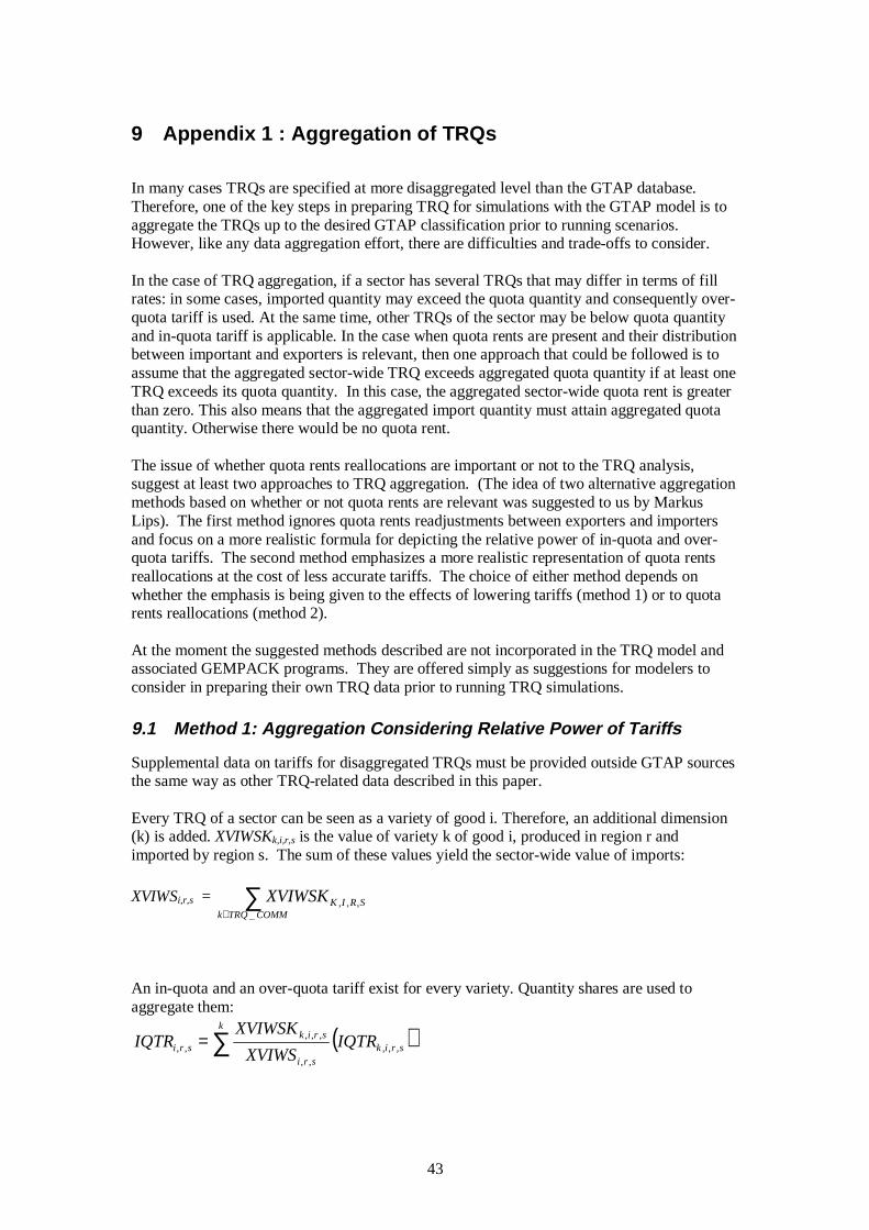
43

9 Appendix 1 : Aggregation of TRQs

In many cases TRQs are specified at more disaggregated level than the GTAP database.Therefore, one of the key steps in preparing TRQ for simulations with the GTAP model is toaggregate the TRQs up to the desired GTAP classification prior to running scenarios.However, like any data aggregation effort, there are difficulties and trade-offs to consider.

In the case of TRQ aggregation, if a sector has several TRQs that may differ in terms of fillrates: in some cases, imported quantity may exceed the quota quantity and consequently over-quota tariff is used. At the same time, other TRQs of the sector may be below quota quantityand in-quota tariff is applicable. In the case when quota rents are present and their distributionbetween important and exporters is relevant, then one approach that could be followed is toassume that the aggregated sector-wide TRQ exceeds aggregated quota quantity if at least oneTRQ exceeds its quota quantity. In this case, the aggregated sector-wide quota rent is greaterthan zero. This also means that the aggregated import quantity must attain aggregated quotaquantity. Otherwise there would be no quota rent.

The issue of whether quota rents reallocations are important or not to the TRQ analysis,suggest at least two approaches to TRQ aggregation. (The idea of two alternative aggregationmethods based on whether or not quota rents are relevant was suggested to us by MarkusLips). The first method ignores quota rents readjustments between exporters and importersand focus on a more realistic formula for depicting the relative power of in-quota and over-quota tariffs. The second method emphasizes a more realistic representation of quota rentsreallocations at the cost of less accurate tariffs. The choice of either method depends onwhether the emphasis is being given to the effects of lowering tariffs (method 1) or to quotarents reallocations (method 2).

At the moment the suggested methods described are not incorporated in the TRQ model andassociated GEMPACK programs. They are offered simply as suggestions for modelers toconsider in preparing their own TRQ data prior to running TRQ simulations.

9.1 Method 1: Aggregation Considering Relative Power of Tariffs

Supplemental data on tariffs for disaggregated TRQs must be provided outside GTAP sourcesthe same way as other TRQ-related data described in this paper.

Every TRQ of a sector can be seen as a variety of good i. Therefore, an additional dimension(k) is added. XVIWSKk,i,r,s is the value of variety k of good i, produced in region r andimported by region s. The sum of these values yield the sector-wide value of imports:

XVIWSi,r,s = ∑∈ COMMTRQk

SRIKXVIWSK_

,,,

An in-quota and an over-quota tariff exist for every variety. Quantity shares are used toaggregate them:

( )∑=k

sriksri

sriksri IQTR

XVIWS

XVIWSKIQTR ,,,

,,

,,,,,

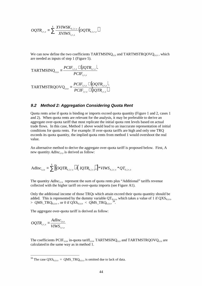
44

( )∑=k

sriksri

sriksri OQTR

XVIWS

XVIWSKOQTR ,,,

,,

,,,,,

We can now define the two coefficients TARTMSINQi,r,s and TARTMSTRQOVQi,r,s , whichare needed as inputs of step 1 (Figure 5).

( )sri

srisri

PCIF

IQTRPCIF

,,

,,,,r,si,TARTMSINQ

+=

( )( )srisri

srisri

IQTRPCIF

OQTRPCIF

,,,,

,,,,r,si,VQTARTMSTRQO

++

=

9.2 Method 2: Aggregation Considering Quota Rent

Quota rents arise if quota is binding or imports exceed quota quantity (Figure 1 and 2, cases 1and 2). When quota rents are relevant for the analysis, it may be preferable to derive anaggregate over-quota tariff that most replicate the initial quota rent levels based on actualtrade flows. In this case, Method 1 above would lead to an inaccurate representation of initialconditions for quota rents. For example: If over-quota tariffs are high and only one TRQexceeds its quota quantity, the implied quota rents from method 1 would overshoot the realvalue.

An alternative method to derive the aggregate over-quota tariff is proposed below. First, Anew quantity AdInci,r,s is derived as follow:

( ) ( )[ ] sriksrik

k

sriksrik QTVIWSIQTROQTR ,,,,,,,,,,,,sr,i, **AdInc ∑ −=

The quantity AdInci,r,s represent the sum of quota rents plus “Additional” tariffs revenuecollected with the higher tariff on over-quota imports (see Figure A1).

Only the additional income of those TRQs which attain exceed their quota quantity should beadded. This is represented by the dummy variable QTk,i,r,s which takes a value of 1 if QXSk,i,r,s

> QMS_TRQk,i,r,s , or 0 if QXSk,i,r,s < QMS_TRQk,i,r,s 34.

The aggregate over-quota tariff is derived as follow:

sri

sr,i,sri

VIWS

AdIncOQTR

,,,, =

The coefficients PCIFi,r,s, in-quota tariffi,r,s, TARTMSINQi,r,s and TARTMSTRQOVQi,r,s arecalculated in the same way as in method 1.

34 The case QXSk,i,r,s = QMS_TRQk,i,r,s is omitted due to lack of data.

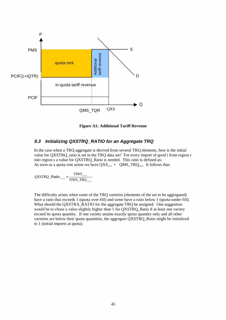
45

Figure A1: Additional Tariff Revenue

9.3 Initializing QXSTRQ_RATIO for an Aggregate TRQ

In the case when a TRQ aggregate is derived from several TRQ elements, how is the initialvalue for QXSTRQ_ratio is set in the TRQ data set? For every import of good i from region rinto region s a value for QXSTRQ_Ratio is needed. This ratio is defined as:As soon as a quota rent arises we have QXSi,r,s • QMS_TRQi,r,s. It follows that:

sri

srisri VIWS_TRQ

VIWSQXSTRQ_

,,

,,,, =Ratio

The difficulty arises when some of the TRQ varieties (elements of the set to be aggregated)have a ratio that exceeds 1 (quota over-fill) and some have a ratio below 1 (quota-under-fill).What should the QXSTRA_RATIO for the aggregate TRQ be assigned. One suggestionwould be to chose a value slightly higher than 1 for QXSTRQ_Ratio if at least one varietyexceed its quota quantity. If one variety attains exactly quota quantity only and all othervarieties are below their quota quantities, the aggregate QXSTRQ_Ratio might be initializedto 1 (initial imports at quota).

Add

ition

alta

riff r

even

uePCIF

PMS

QMS_TQR

quota rent

in-quota tariff revenue

P

Q

S

DPCIF(1+IQTR)

QXS

46

10 Appendix 2 : Equation E_TMS in GTAPxTRQ.TAB

This is a technical section which you do not need to understand in order to use the TRQmodule supplied with this paper.

As explained in section 3.1 , the levels version of the equation E_TMS is:

IF(TMSTRQ + QXSTRQ_RATIO <= 2, TMSTRQ = 1),ELSE IF(TMSTRQ + QXSTRQ_RATIO >= 1 + TMSTRQOVQ, TMSTRQ = TMSTRQOVQ),ELSE IF(TMSTRQ + QXSTRQ_RATIO > 2 and TMSTRQ + QXSTRQ_RATIO < 1+TMSTRQOVQ, QXS = QMS_TRQ).

In the TRQ module, we have added an extra term to this equation. For triples (i,r,s) with noimports (that is, VIWS = 0), it does not make sense to implement the above behavior. Ratherwe have chosen to hold the actual power of the tariff TMS fixed. [This has no effect on TRQssince there are no imports, nor will there be any during the application.]

The three conditions in the equation above are there to tell us the position of the point inrelation to LINE A and LINE B in Figure 3. In the TRQ module, we have introduced aCoefficient called TRQPOS whose value indicates the position of the point in relation to theselines (see Figure 3). Thus the actual levels equation has the form

IF(VIWS <= SMALL_VIWS, TMS is constant),ELSE IF(TRQPOS = -1, TMSTRQ = 1),ELSE IF(TRQPOS = 1, TMSTRQ = TMSTRQOVQ),ELSE IF(TRQPOS = 0, QXS = QMS_TRQ).

where SMALL_VIWS has previously been set equal to zero. The GEMPACK syntax for thisis

IF(VIWS <= SMALL_VIWS, TMS is constant) +IF(VIWS > SMALL_VIWS and TRQPOS = -1, TMSTRQ = 1) +IF(VIWS > SMALL_VIWS and TRQPOS = 1, TMSTRQ = TMSTRQOVQ) +IF(VIWS > SMALL_VIWS and TRQPOS = 0, QXS = QMS_TRQ).

For any triple (i,r,s) only one of the 4 parts applies and the value of the other 3 parts is zero(so that adding the four parts just gives the part which applies).

The linearized version of a sum of “IF” terms such as the above is just the sum of therespective linearized versions of the separate parts, with the conditions still in place. Thus thelinearized version of the above is

IF(VIWS <= SMALL_VIWS, <linearized version of: “TMS is constant”>) +IF(VIWS > SMALL_VIWS and TRQPOS = -1, <linearized version of “TMSTRQ = 1”>) +IF(VIWS > SMALL_VIWS and TRQPOS = 1, <linearized version of “TMSTRQ = TMSTRQOVQ”>) +IF(VIWS > SMALL_VIWS and TRQPOS = 0, <linearized version of “QXS = QMS_TRQ”>).

As explained in Appendix 3 of Bach and Pearson (1996),35 the Newton correctionlinearization of the equation A = 0 is 35 We repeat this here. For an equation

A = 0the Newton correction is to handle the case where (during a multi-step calculation, say) we havewandered off the curve so that the current levels value of A is not zero but has the value E (error) say.Thus we rewrite the equation as

47

c_A + A*del_Newton = 0 (*)

where c_A denotes the change in A and del_Newton is a special linear variable whose valueis set exogenously equal to 1 in every step of a multi-step calculation.36

Hence the linearized version of the levels equation in the TRQ module is

EQUATION (LINEAR) E_TMS (All,i,TRAD_COMM)(All,r,REG)(All,s,REG)IF(VIWS(i,r,s) <= SMALL_VIWS, p_TMS(i,r,s) ) +IF(VIWS(i,r,s) > SMALL_VIWS and TRQPOS(i,r,s) = -1, TMSTRQ(i,r,s)*p_TMSTRQ(i,r,s) + 100*[TMSTRQ(i,r,s)-1]*del_Newton) +IF(VIWS(i,r,s) > SMALL_VIWS and TRQPOS(i,r,s) = 1, TMSTRQ(i,r,s)*p_TMSTRQ(i,r,s) - TMSTRQOVQ(i,r,s)*p_TMSTRQOVQ(i,r,s) + 100*[TMSTRQ(i,r,s)-TMSTRQOVQ(i,r,s)]*del_Newton) +IF(VIWS(i,r,s) > SMALL_VIWS and TRQPOS(i,r,s) = 0, VIWS(i,r,s)*p_QXS(i,r,s) - VIWS_TRQ(i,r,s)*p_QMS_TRQ(i,r,s) + 100*[VIWS(i,r,s)-VIWS_TRQ(i,r,s)]*del_Newton) + tms_slack(i,r,s) = 0 ;

For example, consider the TRQPOS = -1 part. The levels form is TMSTRQ – 1 = 0. Thechange in TMSTRQ is TMSTRQ*p_TMSTRQ/100. Hence, from (*) above, the relevantexpression for the linearization of this part is

TMSTRQ * p_TMSTRQ + 100 * [TMSTRQ – 1] * del_Newton .

[It is ok to multiply this part by 100 (even though other parts of the equation may not be somultiplied) since the RHS is zero.]

Note that the TRQPOS = 0 part is multiplied by 100*PCIF to convert quantities to values (forexample, PCIF*QXS=VIWS).

There is a further term tms_slack(i,r,s) which we have not so far explained. This is a “slack”term added to the equation so that we can “turn the equation off” (that is, effectively remove itfrom the system of equations in operation) by a closure swap. In the approximate simulation(see section 4.1), we want this equation to apply to all triples (i,r,s) which is achieved bysetting all components of the slack variable tms_slack exogenous. This means that the valueof TMS(i,r,s) is set by this equation for all triples (i,r,s). But, in the accurate simulation, weset the TMS(i,r,s) values from our knowledge of the TRQ status (in quota, at quota or overquota) of each triple from the approximate simulation. So this equation E_TMS is turned offby setting all components of tms_slack endogenous. [See the closure swaps for the accuratesimulation in section 4.2.2.]

A = E.

The change linearization of this isc_A = c_E.

The Newton correction comes by taking c_E equal to -A (or -E). Imposing this change on E willhopefully return E to zero (as desired). Thus the Newton correction linearization of A=0 is

c_A = - A or c_A + A = 0.Since this is not a legal GEMPACK linearized equation (the constant term -A is not allowed) weintroduce a special linear variable del_Newton whose value is set exogenously equal to 1 in every stepof a multi-step calculation. This gives us the Newton correction linearization of A=0 as

c_A + A*del_Newton = 0.36 This achieved by declaring del_Newton via the statement

VARIABLE (LINEAR, NO_SPLIT) del_Newton ;