Implementation of Modal Combination Rules for Response ...

UCRL-ID- 1345 11

Implementation of Modal Combination Rules for Response Spectrum Analysis using GEMINI

Phani K. Nukala

June 1999

This is an informal report intended primarily for internal or limited external 7

distribution. The opinions and conclusions stated are those of the author and may or may not be those of the Laboratory. . Work performed under the auspices of the U.S. Department of Energy by the Lawrence Livermore National Laboratory under Contract W-7405ENG-48.

DISCLAIMER

This document was prepared as an account of work sponsored by an agency of the United States Government. Neitherthe United States Government nor the University of California nor any of their employees, makes any warranty, expressor implied, or assumes any legal liability or responsibility for the accuracy, completeness, or usefulness of anyinformation, apparatus, product, or process disclosed, or represents that its use would not infringe privately ownedrights. Reference herein to any specific commercial product, process, or service by trade name, trademark,manufacturer, or otherwise, does not necessarily constitute or imply its endorsement, recommendation, or favoring bythe United States Government or the University of California. The views and opinions of authors expressed herein donot necessarily state or reflect those of the United States Government or the University of California, and shall not beused for advertising or product endorsement purposes.

This report has been reproduceddirectly from the best available copy.

Available to DOE and DOE contractors from theOffice of Scientific and Technical Information

P.O. Box 62, Oak Ridge, TN 37831Prices available from (615) 576-8401, FTS 626-8401

Available to the public from theNational Technical Information Service

U.S. Department of Commerce5285 Port Royal Rd.,

Springfield, VA 22161

Implementation of Modal Combination Rules for Response Spectrum Analysis using GEMINI

Phani Kumar V.V. Nukala

The University of California

Lawrence Livermore National Laboratory

P.O. Box 808

Livermore, CA 94550, USA

1 Introduction

One of the widely used methodologies for describing the behavior of a structural system subjected to seismic excitation is response spectrum modal dynamic analysis. Several modal combination rules are proposed in the literature to combine the responses of individual modes in a response spectrum dynamic analysis. In particular, these modal combination rules are used to estimate the representative maximum value of a particular response of interest for design purposes. Furthermore, these combination rules also provide guidelines for combining the representative maximum values of the response obtained for each of the three orthogonal spatial components of an earthquake. This report mainly focuses on the implementation of different modal combination rules into GEMINI [I].

2 Combination of Modal Responses

The most widely used combination rule for combining the modal responses of individual modes in a response spectrum analysis is the square root of the sum of the squares (SRSS) of the maximum values of the response of individual modes [a]. However, in the case of closely spaced modes, SRSS procedure significantly underestimates the true response [3, 41. Several modal combination rules are proposed in the literature to account for the effect of

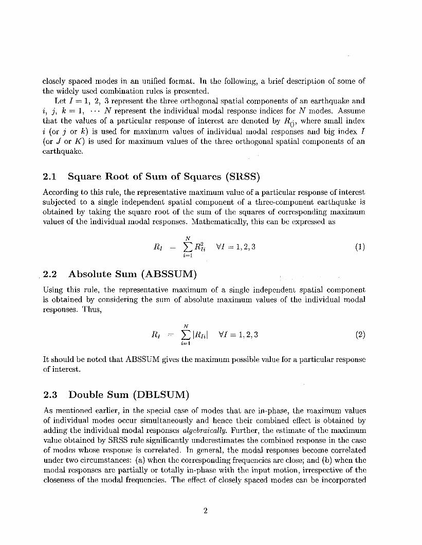
closely spaced modes in an unified format. In the following, a brief description of some of the widely used combination rules is presented.

Let I = 1, 2, 3 represent the three orthogonal spatial components of an earthquake and i, j, k = 1, a- * N represent the individual modal response indices for N modes. Assume that the values of a particular response of interest are denoted by Rtj, where small index i (or j or Ic) is used for maximum values of individual modal responses and big index I (or J or K) is used for maximum values of the three orthogonal spatial components of an earthquake.

2.1 Square Root of Sum of Squares (SRSS)

According to this rule, the representative maximum value of a particular response of interest subjected to a single independent spatial component of a three-component earthquake is obtained by taking the square root of the sum of the squares of corresponding maximum values of the individual modal responses. Mathematically, this can be expressed as

RI = gRii ‘ifI= 1,2,3 (1) i=l

2.2 Absolute Sum (ABSSUM)

Using this rule, the representative maximum of a single independent spatial component is obtained by considering the sum of absolute maximum values of the individual modal responses. Thus,

RI = &Rri, VI= 1,2,3 (2) i=l

It should be noted that ABSSUM gives the maximum possible value for a particular response of interest.

2.3 Double Sum (DBLSUM)

As mentioned earlier, in the special case of modes that are in-phase, the maximum values of individual modes occur simultaneously and hence their combined effect is obtained by adding the individual modal responses algebraically. Further, the estimate of the maximum value obtained by SRSS rule significantly underestimates the combined response in the case of modes whose response is correlated. In general, the modal responses become correlated under two circumstances: (a) when the corresponding frequencies are close; and (b) when the modal responses are partially or totally in-phase with the input motion, irrespective of the closeness of the modal frequencies. The effect of closely spaced modes can be incorporated

2

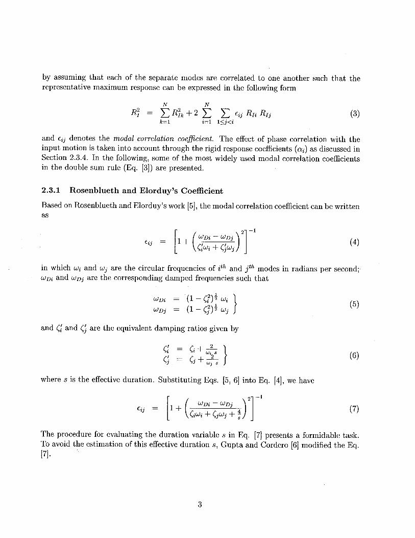
by assuming that each of the separate modes are correlated to one another such that the representative maximum response can be expressed in the following form

R; = 5 R;k + 2 fl: c cij RIi R, k=l i=l l<j<i

(3)

and Eij denotes the modal correlation coeficient. The effect of phase correlation with the input motion is taken into account through the rigid response coefficients (ai) as discussed in Section 2.3.4. In the following, some of the most widely used modal correlation coefficients in the double sum rule (Eq. [3]) are presented.

2.3.1 Rosenblueth and Elorduy’s Coefficient

Based on Rosenblueth and Elorduy’s work [5], the modal correlation coefficient can be written as

in which wi and tij are the circular frequencies of ith and jth modes in radians per second; wgi and WDj are the corresponding damped frequencies such that

WDi = (1 -c,“)i wi

WDj = (1-c;); Wj (5)

and [i and 5; are the equivalent damping ratios given by

where s is the effective duration. Substituting Eqs. [5, 61 into Eq. [4], we have

2 )I -1

Eij = WDi - WDj

CiWi + <jWj + f

(6)

(7)

The procedure for evaluating the duration variable s in Eq. [7] presents a formidable task. To avoid the estimation of this effective duration s, Gupta and Corder0 [6] modified the Eq. [7]. (,

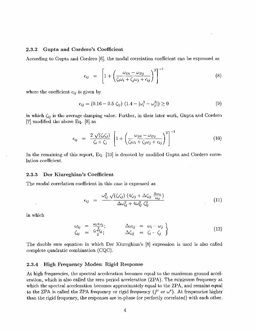
2.3.2 Gupta and Cordero’s Coefficient

According to Gupta and Corder0 [6], the modal correlation coefficient can be expressed as

2 )I -1

Eij = WDi - WDj

[iWi + <jWj + Gj (8)

where the coefficient cij is given by

Cij = (0.16 - O-5 [ij) (I.4 - 1w.f - W;[) 2 0 (9)

in which <ij is the average damping value. Further, in their later work, Gupta and Corder0 [7] modified the above Eq. [8] as

2 )I -1

Eij = WDi - WDj

<@i + cj Wj + Cij (10)

In the remaining of this report, Eq. [lo] is denoted by modified Gupta and Corder0 correlation coefficient.

2.3.3 Der Kiureghian’s Coefficient

The modal correlation coefficient in this case is expressed as

in which

Wij = wi +q.

cij = G$L;’ Aw,j = wi - wi A& = Ci - Cj (12)

The double sum equation in which Der Kiureghian’s [8] expression is used is also called complete quadratic combination (CQC).

2.3.4 High Frequency Modes: Rigid Response

At high frequencies, the spectral acceleration becomes equal to the maximum ground acceleration, which is also called the zero period acceleration (ZPA). The minimum frequency at which the spectral acceleration becomes approximately equal to the ZPA, and remains equal to the ZPA is called the ZPA frequency or rigid frequency (f’ or w’). At frequencies higher than the rigid frequency, the responses are in-phase (or perfectly correlated) with each other.

4

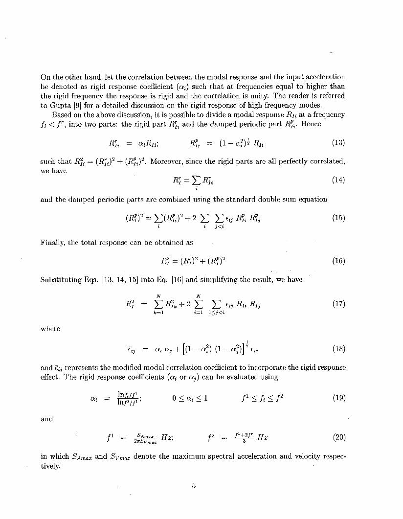
On the other hand, let the correlation between the modal response and the input acceleration be denoted as rigid response coefficient (ai) such that at frequencies equal to higher than the rigid frequency the response is rigid and the correlation is unity. The reader is referred to Gupta [9] for a detailed discussion on the rigid response of high frequency modes.

Based on the above discussion, it is possible to divide a modal response Rli at a frequency fi < f’, into two parts: the rigid part RFi and the damped periodic part R~i. Hence

Rli = aiRri; RTi = (1 - C# Rli (13)

such that R;i = (R;J2 + (RTi)2. M oreover, since the rigid parts are all perfectly correlated, we have

R;=CRTi (14 i

and the damped periodic parts are combined using the standard double sum equation

(Ry)2 = C(Ryi)2 + 2 C Ctij RTi R~i (15) i i j<i

Finally, the total response can be obtained as

R; = (R;)2 + (R;)2 (16)

Substituting Eqs. [13, 14, 151 into Eq. [16] and simplifying the result, we have

R; = 2 Rik + 2 2 C Eij Rli R, k=l i=l l<j<i -

where

-

Eij = Qi O!j + [(l - d!:) (1 - CXT)]’ Cij

(17)

and Cij represents the modified modal correlation coefficient to incorporate the rigid response effect. The rigid response coefficients (ai or aj) can be evaluated using

Qi = p&. 1’

and

f1 = * Hz;

.fl 5 fi 5 f2

f2 = w Hz

(1%

PO> in which ~~~~~ and Svmaz denote the maximum spectral acceleration and velocity respectively.

5

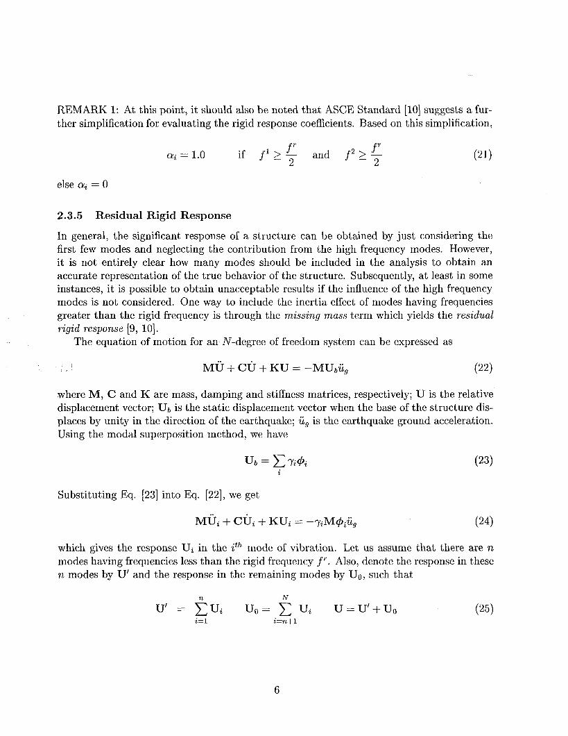
REMARK 1: At this point, it should also be noted that ASCE Standard [lo] suggests a further simplification for evaluating the rigid response coefficients. Based on this simplification,

Qli = 1.0 if f1 2 f and f2 2 f (21)

else pi = 0

2.3.5 Residual Rigid Response

In general, the significant response of a structure can be obtained by just considering the first few modes and neglecting the contribution from the high frequency modes. However, it is not entirely clear how many modes should be included in the analysis to obtain an accurate representation of the true behavior of the structure. Subsequently, at least in some instances, it is possible to obtain unacceptable results if the influence of the high frequency modes is not considered. One way to include the inertia effect of modes having frequencies greater than the rigid frequency is through the missing muss term which yields the residual rigid response [9, lo].

The equation of motion for an N-degree of freedom system can be expressed as

: Mti + Cti + KU = -MU& (22)

where M, C and K are mass, damping and stiffness matrices, respectively; U is the relative displacement vector; Ub is the static displacement vector when the base of the structure dis- places by unity in the direction of the earthquake; ii, is the earthquake ground acceleration. Using the modal superposition method, we have

Substituting Eq. [23] into Eq. [22], we get

which gives the response Ui in the ith mode of vibration. Let us assume that there are n modes having frequencies less than the rigid frequency f ‘. Also, denote the response in these n modes by U’ and the response in the remaining modes by Uo, such that

U’ = eui U(J = 5 Ui u=u’+uo i=l i=n+l

(25)

6

Using Eqs. [22, 24, 251, it is possible to obtain

Moo + Cti, + KU0 = -MU&, (26)

and n

UbO = Ub - c w& (27) i=l

As the response of the structure in modes having frequencies greater than the rigid frequency is pseudo-static, we have

KU0 = -MUboG, =+ U. = -K-‘MUbofi, (28)

Hence the maximum residual rigid response is obtained as

uo max = -K-lMUbo(ZPA) (29)

2.4 Grouping Method

Using this combination rule, closely spaced modes are divided into groups that include all modes having frequencies between the lowest frequency in the group and a frequency 10 % higher. The representative maximum value of a group is obtained by taking the sum of the absolute values of the corresponding maximum individual modal values of that group. Further, the representative maximum value of a particular response is obtained by taking the square root of the sum of the squares of the corresponding representative maximums of all the groups. Mathematically, this can be expressed as follows:

Assume that the modes can be grouped into p individual groups such that no one frequency is in more than one group. Also, assuming that 1 and m denote the lowest and highest frequency modes in the qth group, the representative maximum of each group is obtained as

Using the SRSS rule for combining the group responses, we have

Rf = k=l; kq’P q=l

Substituting Eq. [30] into Eq. [31] and simplifying the result,

Rf = eR;k+f:gF/RIqi Rlqj/ i#.i k=l q=l i=l j=l

(32)

7

which can be re casted into the following double sum rule form as

where Sij can be represented in a sparse matrix format. Precisely, it is this sparse matrix format of iZij that is responsible for representing the double sum rule and grouping method in an unified framework. In the following, the above procedure is illustrated using an example.

Consider a total number of seven frequencies (N = 7) grouped into three groups (p = 3) such that

g1 = W,3); 92 = {4,5); 93 = {6,7)

The corresponding Zij sparse matrix for the above grouping can be represented as

y 11 0 0 0 oT \10000

\oooo [&j] = \ 100

sym\OO \ 1

\-

2.5 Ten Percent Method

Using this combination rule, the representative maximum can be obtained as

Ri=ihk+2 yxjRIi RIjI k=l i j>i

(34)

where the second summation is performed over all i and j modes whose frequencies are closely spaced to each other, i.e., two modes with frequencies are tii and wj are closely spaced, if

Wj - Wi 5 0.1 and

Wi l<i<jlN

Similar to Eq. [32], Eq. [34] can also be re casted into double sum form as

Rf = FRyk-I-2 CClcijRliRIjj k=l i j>i

(36)

8

Once again, let us consider a total of seven frequencies (N = 7). These seven frequencies can be grouped as

91 = W,3h 92 = c&3); Q3 = (374); 94 = {4,5,6)

The corresponding cij sparse matrix for the above grouping can be represented as

[Gj] - -

-\110000 \10000

\ 1000 \llO

sym\lO \ 0

Thus, grouping method and ten percent method can be treated in an unified double sum rule form.

‘* 2.e. : Combination of Spatial Components

In the previous Sections 2.1-2.5, the modal combination rules for a single orthogonal component of an earthquake are presented. In the following, evaluation of the representative maximum response value from the three orthogonal individual spatial components is presented.

When responses from the three earthquake components are calculated separately, the combined earthquake response is obtained by using the square root of the sum of the squares of individual spatial component representative maximum responses, i.e.,

where R is any response of interest and RI is the representative maximum response in the Ith direction and is obtained by using any of the modal combination rules discussed through Sections 2.1-2.5.

3 Some Remarks on Modal Combination Rules

3.1 C&e 1: Residual rigid response as an additional mode

Consider an N degree of freedom structure with a total number N modes. Let us assume that there are n modes having frequencies less than the rigid frequency f’. Also, let RIO

9

denote the residual rigid response due to the high frequency modes. As mentioned earlier, for modes with frequencies equal to or greater than the rigid frequency f’, the responses are in- phase with each other, i.e., the responses are perfectly correlated. Hence the representative maximum due to these modes is given by

R;=Rro+~R;i i=l

(38)

Using Eqs. [3, 13, 15, 161, the representative maximum can be obtained as

R; = (R;)2 + (R;)2 (39)

= R;o + 2 RIO 2 Rl;i + 2 R~i + 2 2 C Cij RIi Rlj I

(40) i=l i=l i=l l<j<i

n+l n+l

= C Rsi + 2 C C 6j RIG RIG 3

(41) i=l i=l l<j<i

where (n + I)th mode is the residual rigid response mode with frequency equal to ZPA, i.e., 0!,+1 = 1.0 ‘. REMARK 2: It should be noted that the above result is identical to the suggested procedure by ASCE Standard [lo] for including the residual rigid response, i.e., residual rigid response can be treated as an’additional mode having a frequency equal to the ZPA or cutoff frequency.

3.2 Case 2: Response of m modes with frequencies fi 2 f’

Now, let us consider that there are m additional modes whose frequency is greater than the cutoff frequency. In such a case,

CYi = 1.0 V i E (n -I 1, n + 2,. . . , n -k m) (42)

and the modes are perfectly correlated, i.e.,

2ij = 1.0 Vi, j E {n+l,n+2;.-,n+m} (43)

Using the double sum rule, the representative maximum response can be obtained as

n+m+l n+m+l R; = C R3i +2 C C Gj RIi RIj (44

i=l i=l l<j<i 1 10

where (n + m + l)th mode is the rigid response mode and Rl~~+~+l) = RIO. Substituting Eqs. [42, 431 into Eq. [44] an simplifying the result, we have d

R; = Rise + 2 R1sO 2 R;i + i=l

where

2 Rpi + 2 2 C Sij Rli Rlj 1

(45) i=l i=l l<j<i

ntm RI~O = RIO + C RIi (46)

i=n+l

REMARK 3: Based on the above derivation, it should be clear that the above result is identical to the procedure suggested by ASCE Standard [lo] for assigning the rigid response coefficients as

Cyi = 0 if fi < f’ (47) =l if fi 2 f’ (48)

and treating the m additional modes as a single mode whose representative maximum is obtained by simply summing the corresponding maximum values of m individual modes. Based on REMARK 2, it is clear that residual rigid response can also be treated as a mode whose frequency is equal to the ZPA or cutoff frequency.

4 Numerical Example

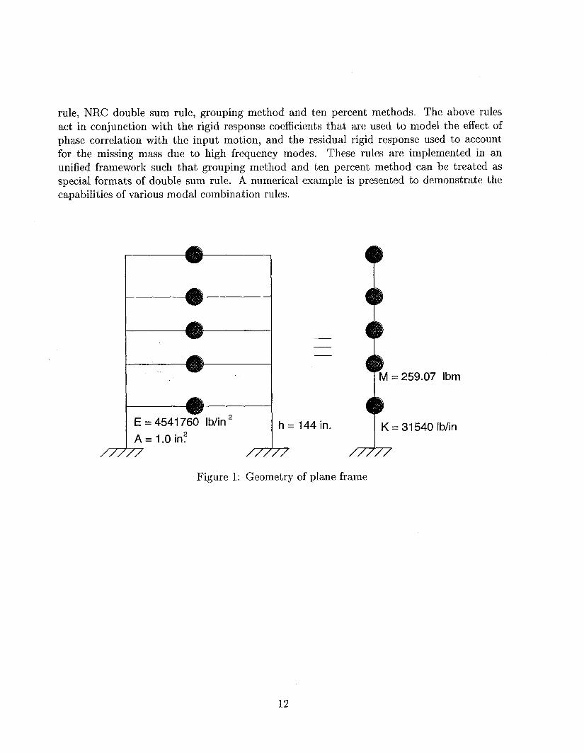
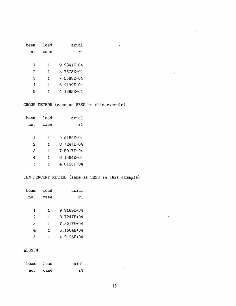
A five story plane frame with geometric and material properties as shown in Fig. [l] is subjected to a seismic loading obtained from El-Centro 1940 earthquake. The plane frame is idealized assuming that the mass of the entire story is located at the center of the slab using a lumped spring-mass idealization. The mass and stiffness properties of the idealized structure are shown in Fig. [l]. The input data deck for an eigenvalue solution and response spectrum analysis of the problem under consideration is given in Appendix I. The output obtained through various modal combination rules with or without residual rigid responses is given in Appendix II. The modified input documentation for response spectrum analysis using GEMINI is given in Appendix III. The reader is also referred to the previous GEMINI [l] documentations for better understanding of the input variables.

5 Summary

This report presents the implementation of several modal combination rules for response spectrum dynamic analysis using GEMINI. The modal combination rules include the widely used square root of the sum of the squares (SRSS) rule, absolute sum rule, double sum

11

rule, NRC double sum rule, grouping method and ten percent methods. The above rules act in conjunction with the rigid response coefficients that are used to model the effect of phase correlation with the input motion, and the residual rigid response used to account for the missing mass due to high frequency modes. These rules are implemented in an unified framework such that grouping method and ten percent method can be treated as special formats of double sum rule. A numerical example is presented to demonstrate the capabilities of various modal combination rules.

259.07 Ibm

K = 31540 lb/in

Figure 1: Geometry of plane frame

12

References

[I] R.C. Murray. “GEMINI: A Computer Program for Two and Three Dimensional Linear Static, and Seismic Structural Analysis”. Rept. ucid-20338, University of California, Lawrence Livermore National Laboratory, 1984.

[2] Newmark N.M. Earthquake Engineering. Prentice-Hall, Inc., Englewood Cliffs, N.J., 1970.

[3] S.L. Singh, A.K. Chu and S. Singh. “Influence of Closely Spaced Modes in Response Spectrum Method of Analysis”. Proceedings of the Specialty Conference on Structural Design of Nuclear Plant Facilities, 2, ASCE, Chicago, IL, 1973.

[4] M. Chu, S.L. Amin and S. Singh. “Spectral Treatment of Actions of Three Earthquake Components on Structures”. Nuclear Engineering and Design, 21, p 126-136, 1993.

[5] E. Rosenblueth and J. Elorduy. “Response of Linear Systems to Certain Transient Disturbances”. Proceedings, Fourth World Conference on Earthquake Engineering, I, p 821-828, Santiago, Chile, 1969.

[6] A.K. Gupta and K. Cordero. “Combination of Modal Responses”. Transaction, Sixth International Conference on Structural Mechanics in Reactor Technology, Paris, 1981.

[7] A.K. Gupta and D.C. Chen. “A Simple Method for Combining Modal Responses”. Transaction, Seventh International Conference on Structural Mechanics in Reactor Technology, Chicago, 1983.

[8] A. Der Kiureghian. “A Response Spectrum Method for Random Vibrations”. Ucb/eerc- 80/15, Earthquake Engineering Research Center, University of California, Berkeley, CA, 1980.

[9] A.K. Gupta. Response Spectrum Method in Seismic Analysis and Design of Structures. CRC Press, Inc., 1990.

[lo] American Society of Civil Engineering. Standard for the Seismic Analysis of Safety Related Nuclear Structures, 1986.

13

APPENDIX I: Input Deck for Numerical Example

Probleml: Part I --plane frame example - eigenvalue solution 7 I la 1 2 3 4 5 6 7 I 2 5

1 1

0 41 I 1 1 I 1 1 I 1 I I I 1 1 I. I 11111 11111 11111 11111 10 1

4541760 0.3 I

0.0 0.0 0.0 144.0 0.0 0.0 288.0 0.0 0.0 432.0 0.0 0.0 576.0 0.0 0.0 720.0 0.0 0.0 432.0 10.0 0.0

1.0 1.0 1.0

112 7 1.1 2 2 3 7 11 3 3 4 7 11 4 4 5 7 11 5 5 6 7 1.1 5 2 0 259.07 3 0 259.07 4 0 259.07 5 0 259.07 6 0 259.07

-1

14

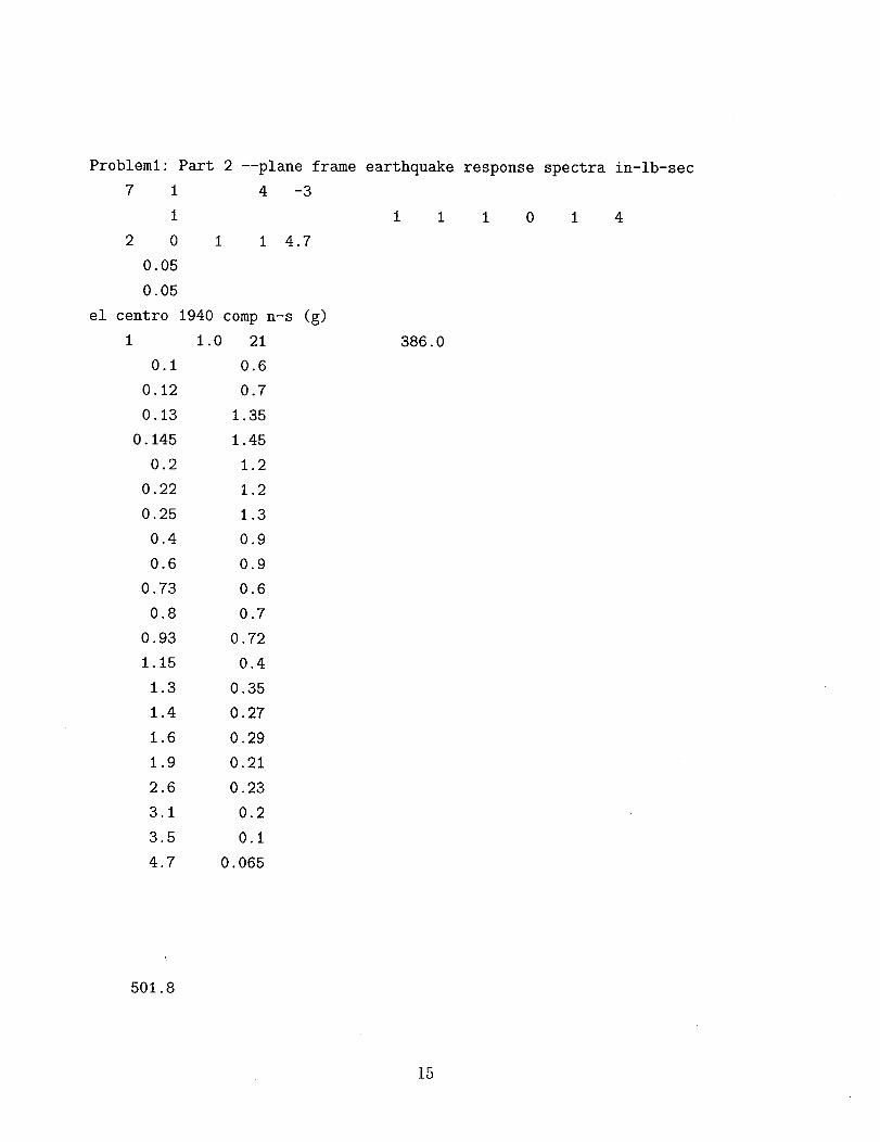
Probleml: Part 2 --plane frame earthquake response spectra in-lb-set 7 1 4 -3

1 1110 14 2 0 1 1 4.7

0.05 0.05

el centro 1940 camp n-s (g) I.

0.1 0.12 0.13

0.145 0.2

0.22 0.25

0.4 0.6

0.73 0.8

0.93 1.15

1.3 1.4 1.6 1.9 2.6 3.1 3.5 4.7

1.0 21 0.6 0.7

1.35 1.45

1.2 1.2 1.3 0.9 0.9 0.6 0.7

0.72 0.4

0.35 0.27 0.29 0.21 0.23

0.2 0.1

0.065

386.0

501.8

15

APPENDIX II: Output

SRSS :

beam load axial no. case rl

1 1 9.9189E+O4 2 1 8.7247E+04 3 1 7.5017E+04 4 1 6.1504E+04 5 1 4.0125E+04

DOUBLE SUM (Gupta and Co) iclose = 1 or 0 => same in this case

beam load no. case

axial rl

1 1 9.9843E+04 2 1 8.7370E+04 3 1 7.486OE+O4 4 1 6.1043E+04 5 1 3.9222E+04

DOUBLE SUM (Rosenblueth and Co) dureff = 4.7 set


1 1 l.O175E+05 2 1 8.7607E+04 3 1 7.4053E+04 4 1 5.9579E+04 5 1 3.7553E+04

16

DOUBLE SUM (cqc)


1 1 9.984lE+04 2 1 8.737OE+O4 3 1 7.486OE+O4 4 1 6.1044E+04 5 1 3.9225E+04

DOUBLE SUM (NRC) (Gupta and Co) iclose = 1 or 0 => same in this case


1 1 9.9843E+O4 2 1 8.7679E+04 3 1 7.5590E+04 4 1 6.2200E+04 5 1 4.1388E+04

DOUBLE SUM (NRC) (Rosenblueth and Co) dureff = 4.7 set


1 1 l.O175E+O5 2 1 8.8562E+04 3 1 7.701lE+04 4 1 6.3970E+04 5 1 4.3560E+04

DOUBLE SUM (NRC) (CQC)

17


1 1 9.984lE+04 2 1 8.7678E+04 3 1 7.5588E+04 4 1 6.2199Ec04 5 1 4.1385E+04

GROUP METHOD (same as SRSS in this example)


1 1 9.9189E+04 2 1 8.7247E+04 3 1 7.5017E+O4 4 1 6.1504E+O4 5 1 4.0125E+04

TEN PERCENT METHOD (same as SRSS in this example)

beam load no. case

1 1 2 1 3 1 4 1 5 1

ABSSUM

axial rl

9.9189E+O4 8.7247E+04 7.5017E+04 6.1504E+04 4.0125E+04


18

1 1 1.4007E+05 2 1 l.l310E+05 3 1 l.O812E+O5 4 1 9.7096E+O4 5 1 7.4865E+04

Rigid Response Coeffcients

------------------------------------------------------------------------------- -------------------------------------------------------------------------------

DOUBLE SUM (Gupta and Co): icorr=O,iclose=l,irrc=i


1 1 9.9844E+O4 2 1 8.7376E+04 3 1 7.4859E+04 4 1 6.1039E+04 5 1 3.9215E+O4

DOUBLE SUM (Rosenblueth and Co) icorr=l,irrc=l


1 1 l.O175E+05 2 1 8.7612E+04 3 1 7.4052E+O4 4 + 1 5.9576E+04 5 1 3.7549E+04

19

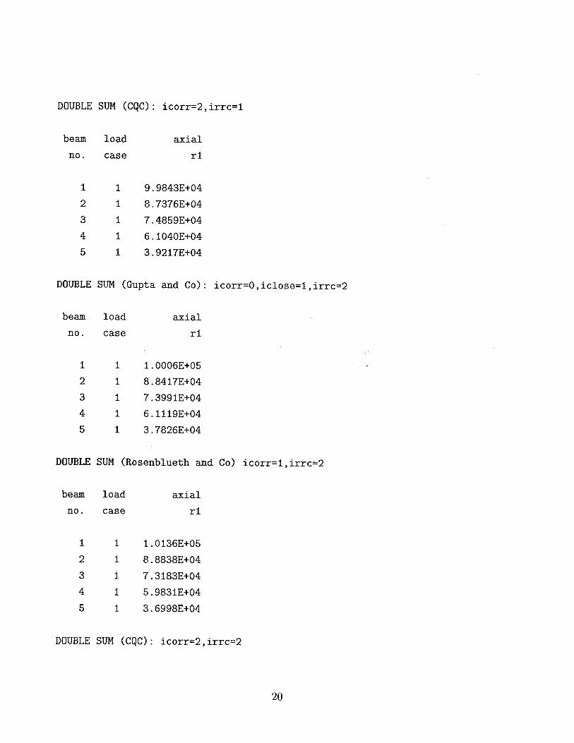
DOUBLE SUM (CQC): icorr=2,irrc=l


1 1 9.9843E+04 2 1 8.7376E+04 3 1 7.4859E+04 4 1 6.1040E+04 5 1 3.9217E+O4

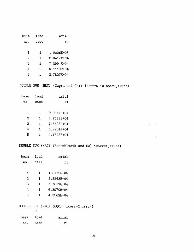
DOUBLE SUM (Gupta and Co): icorr=O,iclose=l,irrc=2


1 1 l.O006E+05 .

2 1 8.8417E+04 3 1 7.3991E+O4 4 1 6.1119E+04 5 1 3.7826E+O4

DOUBLE SUM (Rosenblueth and Co) icorr=l,irrc=2


1 1 l.O136E+05 2 1 8.8838E+04 3 1 7.3183E+04 4 1 5.983lE+04 5 1 3.6998E+04

DOUBLE SUM (CQC): icorr=2,irrc=2

20


1 1 l.O006E+05 2 1 8.8417E+O4 3 1 7.399lE+04 4 1 6.1119E+04 5 1 3.7827E+04

DOUBLE SUM (NRC) (Gupta and Co): icorr=O,iclose=l,irrc=l


1 1 9.9844E+04 2 1 8.7683E+04 3 1 7.5593E+04 4 1 6.2204E+04 5 1 4.1398E+04

DOUBLE SUM (NRC) (Rosenblueth and Co) icorr=l,irrc=l


1 1 l.O175E+O5 2 1 8.8563E+04 3 1 7.7012E+04 4 1 6.3970E+04 5 1 4.3562E+04

DOUBLE SUM (NRC) (CQC): icorr=2,irrc=l


21

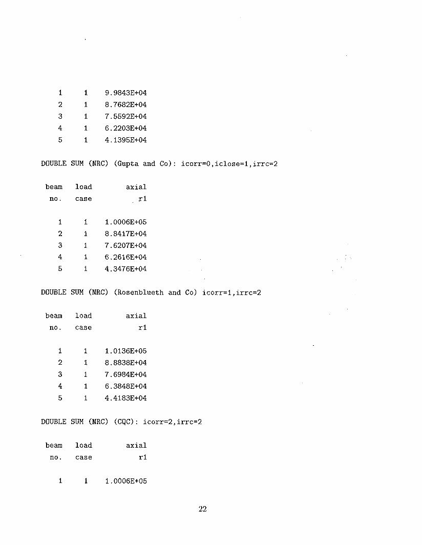
I 1 9.9843E+04 2 1 8.7682E+04 3 1 7.5592E+04 4 1 6.2203E+04 5 1 4.1395E+04

DOUBLE SUM (NRC) (Gupta a.nd Co): icorr=O,iclose=l,irrc=2


1 1 l.O006E+05 2 1 8.8417E+04 3 1 7.6207E+04 4 1 6.2616E+04 5 1 4.3476E+04

DOUBLE SUM (NRC) (Rosenblueth and Co) icorr=l,irrc=2


1 1 l.O136E+05 2 1 8.8838E+04 3 1 7.6984E+O4 4 1 6.3848E+04 5 1 4.4183E+O4

DOUBLE SUM (NRC) (CQC): icorr=2,irrc=2


1 1 l.O006E+05

22

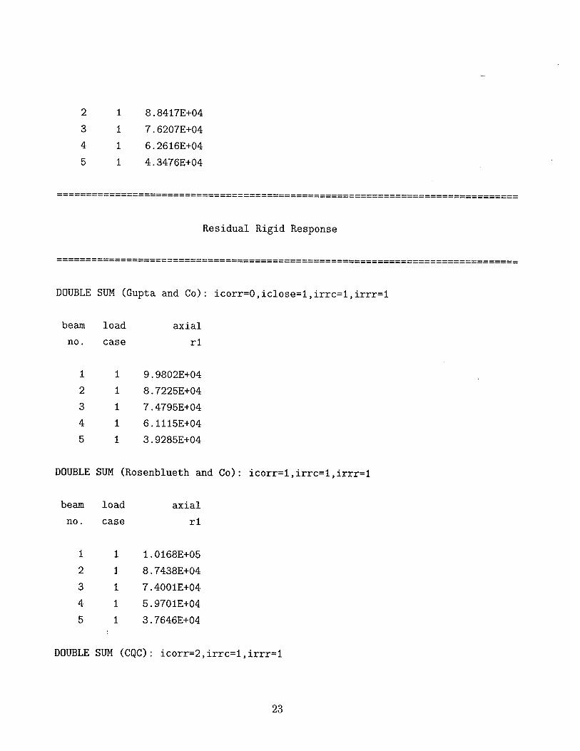
2 1 8.8417E+04 3 1 7.6207E+04 4 1 6.2616E+04 5 1 4.3476E+04

-------------_----------------------------------------------------------------- -----------------_-------------------------------------------------------------

Residual Rigid Response

------------------------------------------------------------------------------- -------------------------------------------------------------------------------

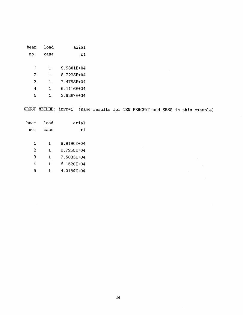
DOUBLE SUM (Gupta and Co): icorr=0,iclose=l,irrc=l,irrr=l


1 1 9.9802E+04 2 1 8.7225E+04 3 1 7.4795E+04 4 1 6.1115E+O4 5 1 3.9285E+04

DOUBLE SUM (Rosenblueth and Co): icorr=l,irrc=l,irrr=l


1 1 l.O168E+05 2 1 8.7438E+04 3 1 7.4001E+04 4 1 5.970lE+04 5 1 3.7646E+04

DOUBLE SUM (CQC): icorr=2,irrc=l,irrr=l

23


1 1 9.9801E+04 2 1 8.7225E+04 3 1 7.4795E+04 4 1 6.1116E+04 5 1 3.9287E+04

GROUP METHOD: irrr=l (same results for TEN PERCENT and SRSS in this example)


1 1 9.919OE+O4 2 1 8.7255E+O4 3 1 7.5033E+O4 4 1 6.152OE+O4 5 1 4.0134E+04

24

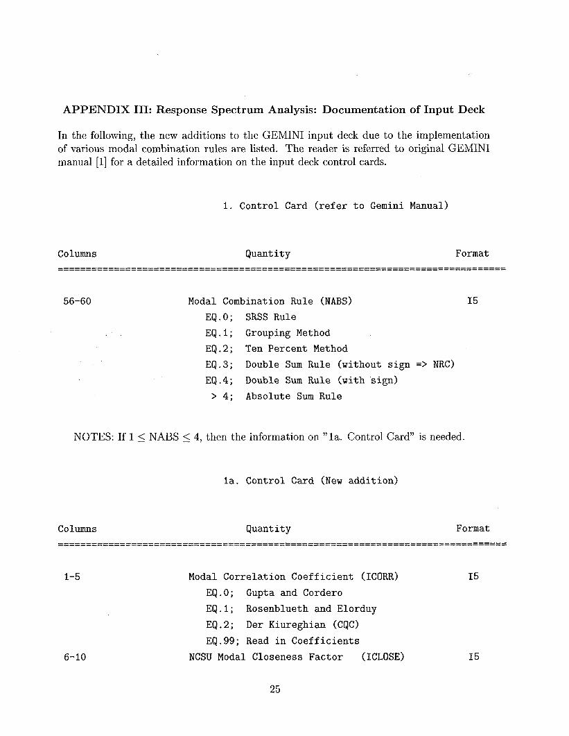
APPENDIX III: Response Spectrum Analysis: Documentation of Input Deck

In the following, the new additions to the GEMINI input deck due to the implementation of various modal combination rules are listed. The reader is referred to original GEMINI manual [l] for a detailed information on the input deck control cards.

I. Control Card (refer to Gemini Manual)

Columns Quantity Format -----------_------------------------------------------------------------------- -------------------------------------------------------------------------------

56-60 Modal Combination Rule (NABS) 15 EQ.0; SRSS Rule EQ.1; Grouping Method EQ.2; Ten Percent Method EQ.3; Double Sum Rule (without sign => NRC) EQ.4; Double Sum Rule (with sign)

> 4; Absolute Sum Rule

NOTES: If 1 5 NABS < 4, then the information on “la. Control Card” is needed.

la. Control Card (New addition)

l-5

6-10

Modal Correlation Coefficient (ICORR) EQ.O; Gupta and Corder0 EQ.1; Rosenblueth and Elorduy EQ.2; Der Kiureghian (CQC) EQ.99; Read in Coefficients

NCSU Modal Closeness Factor (ICLOSE)

15

15

25

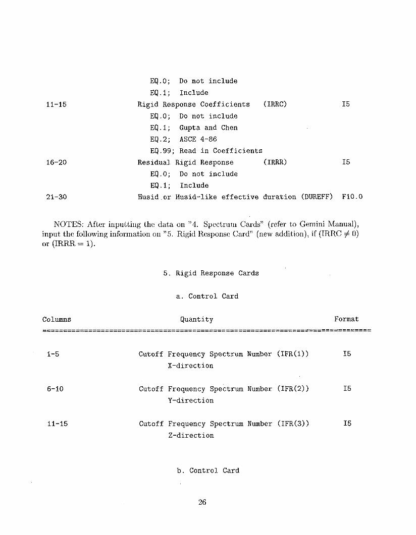
Ii-15

16-20

21-30

15

EQ.O; Do not include EQ.1; Include

Rigid Response Coefficients (IRRC) EQ.O; Do not include EQ.1; Gupta and Chen EQ.2; ASCE 4-86 EQ.99; Read in Coefficients

Residual Rigid Response (IRRR) 15 EQ.O; Do not include EQ.1; Include

Husid.or Husid-like effective duration (DUREFF) FlO.0

NOTES: After inputting the data on “4. Spectrum Cards” (refer to Gemini Manual), input the following information on ” 5. Rigid Response Card” (new addition), if (IRRC # 0) or (IRRR = 1).

5. Rigid Response Cards

a. Control Card

Columns Quantity Format ------------------------------------------------------------------------------- -------------------------------------------------------------------------------

l-5 Cutoff Frequency Spectrum Number (IFR(l)) X-direction

15

6-10

Ii-15

Cutoff Frequency Spectrum Number (IFR(2)) Y-direction

Cutoff Frequency Spectrum Number (IFR(3)) Z-direction

15

15

b. Control Card

26

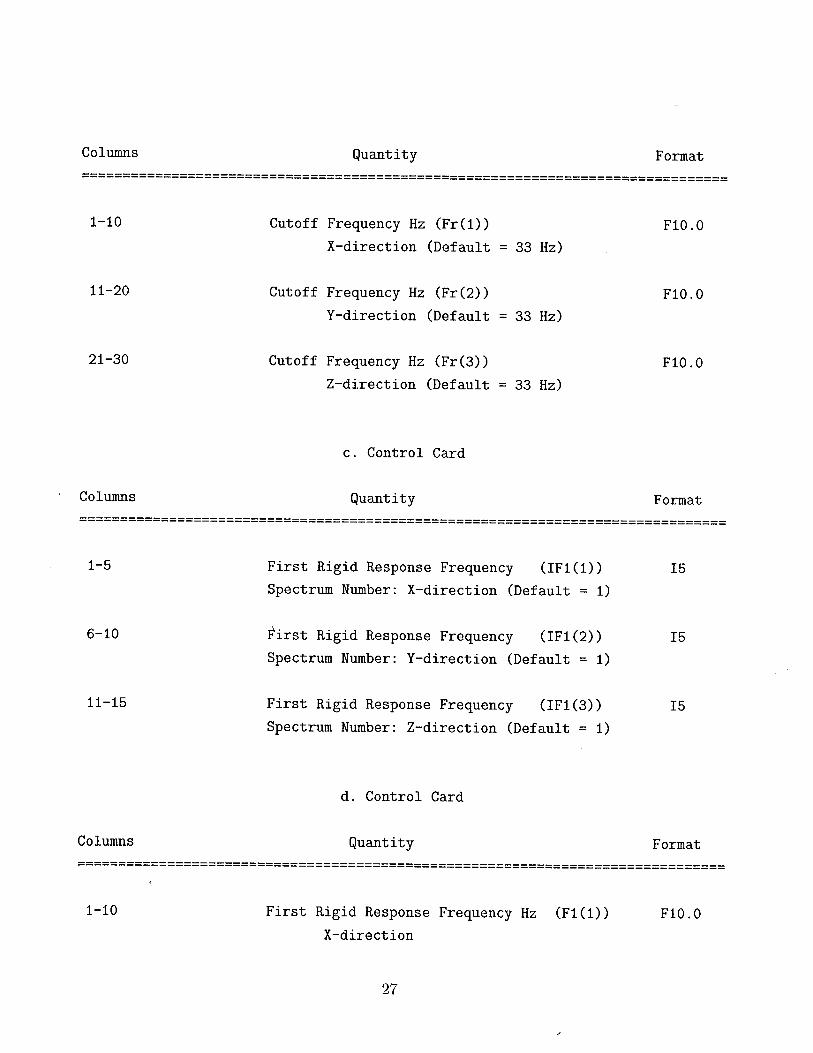
Columns Quantity Format ___-------_-------------------------------------------------------------------- ___----------------------------------------------------------------------------

l-10 Cutoff Frequency Hz (Fr(1)) X-direction (Default = 33 Hz)

F1O.O

Ii-20 Cutoff Frequency Hz (Fr(2)) Y-direction (Default = 33 Hz)

FlO.0

21-30 Cutoff Frequency Hz (Fr(3)) Z-direction (Default = 33 Hz)

F1O.O

c. Control Card

Columns Quantity Format ___----~~~---~~-----~-----~~-----------------------~~-------------~~~---~~~---- ___----~~~---~~~----~-----~------------------~-----~~-------------------~~~----

l-5 First Rigid Response Frequency (IFI( Spectrum Number: X-direction (Default = I)

15

6-10 F\irst Rigid Response Frequency (IFl(2)) Spectrum Number: Y-direction (Default = I)

15

Ii-15 First Rigid Response Frequency (IFl(3)) Spectrum Number: Z-direction (Default = I)

15

d. Control Card

Columns Quantity Format ___---------------------------------------------------------------------------- ___----------------------------------------------------------------------------

l-10 First Rigid Response Frequency Hz (Fl(1)) X-direction

F1O.O

27

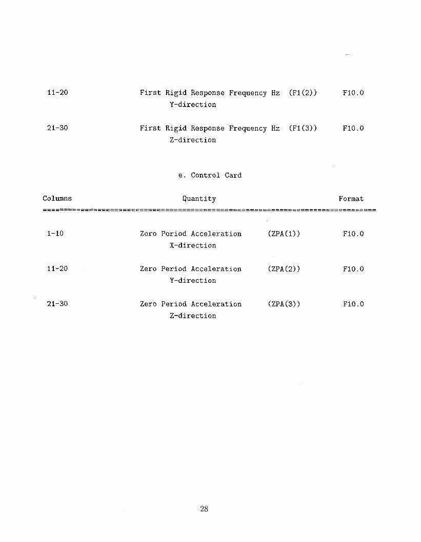
Ii-20

21-30

First Rigid Response Frequency Hz (Fl(2)) FlO.0 Y-direction

First Rigid Response Frequency Hz @ l(3)) FlO.0 Z-direction

e. Control Card

Columns Quantity Format ===============================================================================

l-10 Zero Period Acceleration X-direction

(ZPA(l)) FlO.0

Ii-20 Zero Period Acceleration Y-direction

(ZPA(2)) FlO.0

21-30 Zero Period Acceleration Z-direction

@A(3)) FlO.0

28

Implementation of Modal Combination Rules for Response ...

Documents