Implementation of Finite Element Method with Higher Order Particle Discretization Scheme

Implementation of Finite Element Method with HigherOrder Particle Discretization Scheme

Mahendra Kumar PAL1, Lalith WIJERATHNE2, Muneo HORI3, TsuyoshiICHIMURA4, Seizo TANAKA5

1PhD. Candidate, Department of Civil Engineering, University of Tokyo (Bunkyo, Tokyo 113-0032)E-mail: [email protected]

2Member of JSCE, Assoc. Prof., Earthquake Research Institute, University of Tokyo (Bunkyo, Tokyo 113-0032)E-mail: [email protected]

3Member of JSCE, Prof., Earthquake Research Institute, University of Tokyo (Bunkyo, Tokyo 113-0032)E-mail: [email protected]

4Member of JSCE, Assoc. Prof., Earthquake Research Institute, University of Tokyo (Bunkyo, Tokyo 113-0032)E-mail: [email protected]

5Member of JSCE, Asst. Prof., Earthquake Research Institute, University of Tokyo (Bunkyo, Tokyo 113-0032)E-mail: [email protected]

This paper studies the extension of particle discretization scheme (PDS) in order to improve finite elementmethod implemented with this discretization scheme (PDS-FEM). Polynomials are included in the basisfunctions, while original PDS uses a characteristic function or zero-th order polynomial only. It is shownthat including 1st order polynomials in PDS, the rate of the convergence reaches the value of 2 even forthe derivative. 1st order polynomials are successfully included in PDS-FEM. A numerical experiment iscarried out by applying 1st order PDS-FEM, and the improvement of the accuracy is discussed.

Key Words: particle discretization scheme, higher order extension, Taylor expansion, FEM

1. Introduction

Cracking of solid is a common phenomenon whichleads to failure. It strongly depends on local ma-terial properties, since no identical crack pattern isfound for experimental samples of the same config-uration subjected to the same loading. Also, surfacesof cracks are complicated, as they kink or branch in abulk body.

The numerical analysis of cracking must accountfor the two characteristics, namely, the dependenceon local material heterogeneities and the formation ofcomplicated surfaces. Conventional numerical meth-ods may not be capable of studying these character-istics in an efficient manner, since it is not a simpletask to determine the configuration of the propagat-ing crack surface, which could kink or branch, byconsidering local material heterogeneities. A few re-cent advancements 1),2),3),4),5) have increased the capa-bility of the conventional numerical methods to anal-yse cracking. For instance, a new enhancement istracking of the crack front, which is supported withautomated modification, in simulating the propagat-ing crack. However, objective decision on tracking ofthe crack front is deceptive. Also, this enhancementis computationally expensive and complex in imple-

mentation.Particle Discretization Scheme-Finite Element

Method (PDS-FEM)6),7),8),9) is a new numericalmethod of simulating cracking phenomena, which en-ables us to make simple modelling of the crack sur-face considering material heterogeneities. In PDS,a function is discretized by using the characteris-tic functions of each tessellation, so that a functiondiscretized in PDS allows discontinuities across allneighbouring tessellations. It is rigorously provedthat PDS-FEM has the identical stiffness matrix withlinear element FEM. Hence, cracking is easily treatedas discontinuity of the discretized function, and thereduction of the stiffness due to cracking is rigorouslycomputed.

The limitation of the accuracy that is inherent to thelinear element FEM is shared by PDS-FEM. Thus, theimprovement of the accuracy of PDS-FEM is of pri-mary importance, with the key feature of FEM, thesimple determination of the crack surface consideringmaterial heterogeneities, being preserved as it is. Tothis end, this paper considers higher order PDS. Thebasic idea is to regard PDS as a discretization schemewhich assembles a set of Taylor series expansions. Atarget function is expanded in polynomials in eachtessellation, and these polynomials are connected to

土木学会論文集 A2(応用力学), Vol. 70, No. 2 (応用力学論文集 Vol. 17), I_297-I_305, 2014.

I_297

form a discretized function.It should be emphasized that taking the Taylor

series expansion is most accurate in representing asmooth function locally. The disadvantage of this ex-pansion is that the expanded polynomials do never de-cay near the boundary of the domain of expansion.In higher order PDS, we allow the presence of dis-continuity in neighbouring Taylor series expansions,so that crack surfaces can be simply modelled as theinterface between the neighbouring domains of ex-pansion. The presence of numerous discontinuitiesis a hinge in computing derivatives of a discretizedfunction. In higher-order PDS, derivatives are dis-cretized by using another tessellation, to overcomethis hinge, just as the present PDS employs the conju-gate Voronoi and Delaunay tessellations in discretiz-ing a function and its derivative, respectively.

The contents of this paper are as follows: First, weformulate higher order PDS in Section 2, clarifyingthe discretization of a function and its derivative. Asthe simplest case, 1st order PDS is implemented inFEM in Section 3. A numerical example is solved byusing PDS-FEM, and the improvement of the accu-racy of PDS-FEM is discussed in Sections 4. Someremarks are made in the last section.

The Cartesian coordinate system is used, with indexnotation such as xi, representing the i-th coordinate;summation convention is employed, and an index fol-lowing a comma denotes the partial derivative withrespect to that coordinate. For simpler expressions,symbolic notation is used as well for a vector or ten-sor quantity.

2. Higher order PDS

While any pair of conjugate geometries can be usedfor tessellating an analysis domain, PDS-FEM hasutilized the pair of conjugate Voronoi and Delaunaytessellations; a certain error of discretization identi-cally vanishes for this pair. In this paper, we followthe previous works of PDS-FEM and use conjugateVoronoi and Delaunay tessellations.

Let f be a target function in an analysis domainV . We take conjugate Voronoi and Delaunay tes-sellations, Φα and Ψβ, for this V , and denoteby yα or zβ the mother point of Ψα and the centreof gravity of Ψβ , respectively and denote by ϕα andψβ the characteristic function of Φα and Ψβ , respec-tively.Here,the characteristics function Φα satisfiesΦα(x) = 1 for x ∈ Ωα and = 0 for x ∈ Ωα . Wedefine a discretized function and derivative of f , asfollows:

fd(x) =Nα∑α=1

(N∑

n=0

fαnPn(x− yα)ϕα(x)

), (1)

gdi (x) =

Nβ∑β=1

(N∑

n=0

gβni Pn(x− zβ)ψβ(x)

), (2)

where P0 = 1 and Pn = xn for n = 1, ..., N ofthe N dimension setting, Nα is a number of Voronoitessellations and Nβ is a number of Delaunay tessel-lations. The coefficient fαn is determined by mini-mizing Ef =

∫(f − fd)2 dv, which results into the

following system of equation,∑Iαnαmfαm =

∫Pn(x− yα)ϕα(x)f(x) dv.

(3)Also, the coefficient gβni is determined by minimizingEg =

∫|gd(x) − ∇fd(x)|2 dv with |(.)|2 being the

norm of a vector (.), which results into the followingsystem of equation,∑

Iβnβmgβmi =

∫Pn(x− zβ)ψβ(x)fd,i(x) dv.

(4)Here, by definition, fd,i is expressed in terms of fαnas∑fαn(Pn(x − yα)ϕα(x)),i. Here Iαnαm =∫

Pn(x− yα)Pm(x− yα) dv.As is seen, it is straightforward to include the 1st

order polynomials in the original PDS that uses thecharacteristic functions as the basis functions of dis-cretization. The conversion from the discretized func-tion to the discretized derivative is straightforward aswell, since the closed function (that is measured interms of natural L2) is chosen by minimizing a nat-urally defined error. From now on, we call this PDSas 1st order PDS. Further extension of PDS to higherorder polynomials is also straightforward. Indeed,Eq.(1) or (2) gives an expression of this higher or-der PDS, just by including higher order polynomialsin Pn. The number of the coefficients, however, in-creases as the order of the polynomial increases; forinstance, the number of the coefficients increase from4 to 10 if the second order polynomials are included.

In presenting higher order PDS, the authors use theterm Taylor expansion in a naive sense. As is seen,the coefficients fαn and gβni are not exactly the coef-ficient one would obtain if Taylor series expansion isperformed. However, the higher the order of polyno-mials used in PDS, the closer the coefficients of PDSto that of Taylor expansion. This naive use of Tay-lor expansion makes it easy to deliver a clear mentalimage about the higher order PDS.

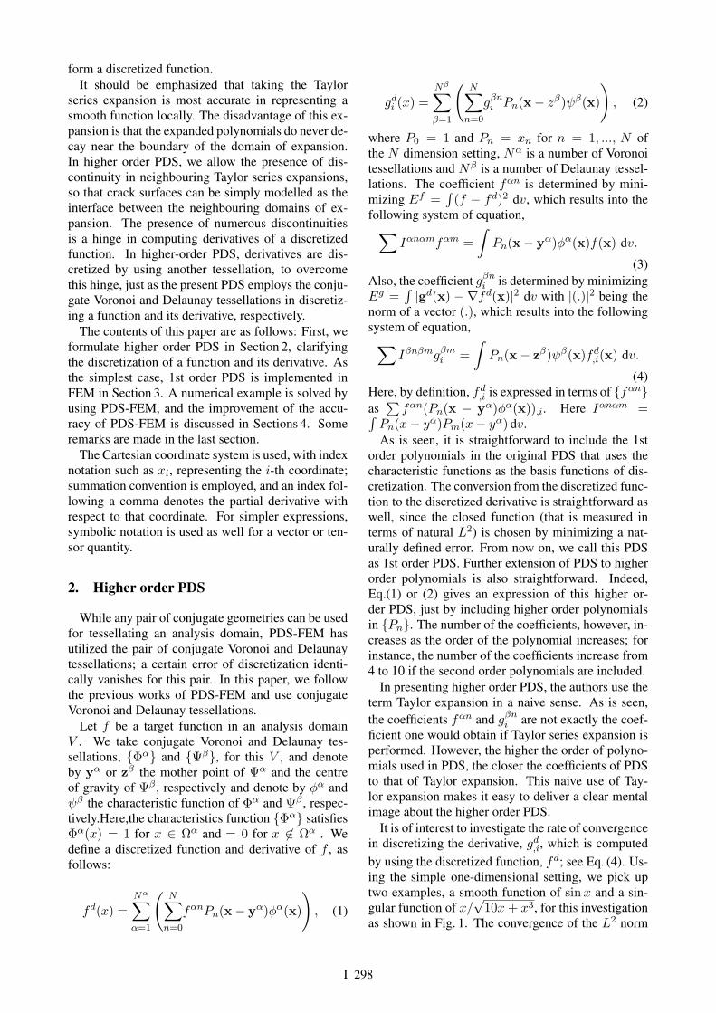
It is of interest to investigate the rate of convergencein discretizing the derivative, gd,i, which is computedby using the discretized function, fd; see Eq. (4). Us-ing the simple one-dimensional setting, we pick uptwo examples, a smooth function of sinx and a sin-gular function of x/

√10x+ x3, for this investigation

as shown in Fig. 1. The convergence of the L2 norm

I_298

1 2 3 4 5

0.15

0.20

0.25

0.30

0.35

0.40

(a)1 2 3 4 5

0.15

0.20

0.25

0.30

0.35

0.40

(b)

1 2 3 4 5

0.05

0.10

0.15

0.20

0.25

0.30

(c)1 2 3 4 5

0.05

0.10

0.15

0.20

0.25

0.30

(d)

Fig.1 (a) & (b) Approximation of function and (c) & (d)its derivative with two different tessellation

0.0625

0.125

0.25

0.5

1

9 36 144

log

2(L

2-n

orm

)

log2(number of DOF)

Sin(x)

f(x)=x ⁄ √(10x+x^3 )

1

1

1.97

2.1

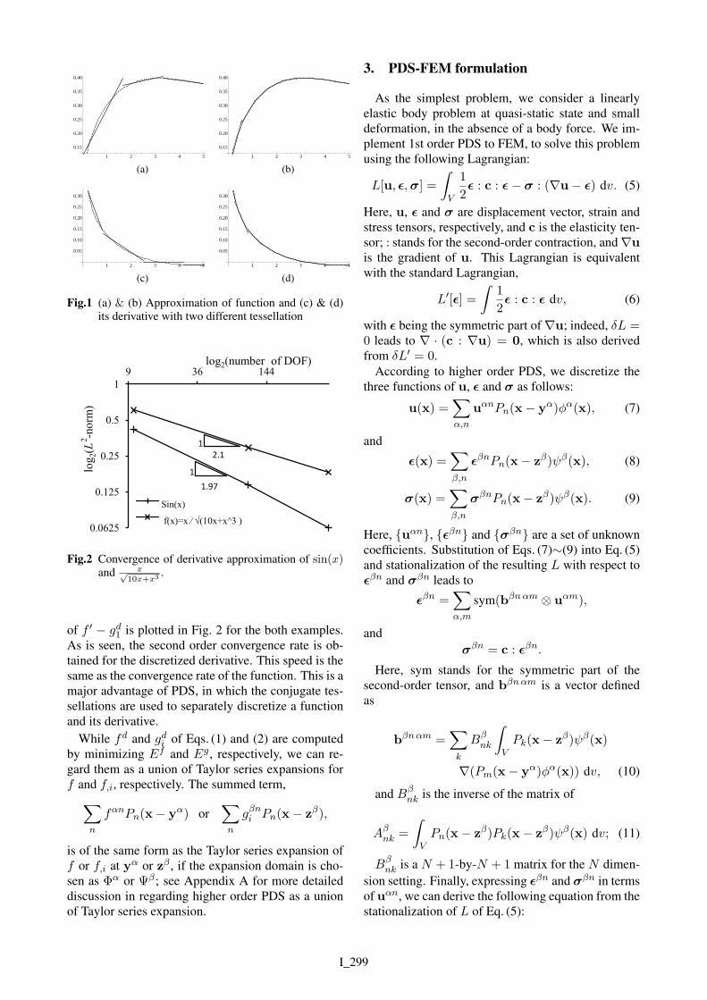
Fig.2 Convergence of derivative approximation of sin(x)and x√

10x+x3.

of f ′ − gd1 is plotted in Fig. 2 for the both examples.As is seen, the second order convergence rate is ob-tained for the discretized derivative. This speed is thesame as the convergence rate of the function. This is amajor advantage of PDS, in which the conjugate tes-sellations are used to separately discretize a functionand its derivative.

While fd and gdi of Eqs. (1) and (2) are computedby minimizing Ef and Eg, respectively, we can re-gard them as a union of Taylor series expansions forf and f,i, respectively. The summed term,∑

n

fαnPn(x− yα) or∑n

gβni Pn(x− zβ),

is of the same form as the Taylor series expansion off or f,i at yα or zβ , if the expansion domain is cho-sen as Φα or Ψβ; see Appendix A for more detaileddiscussion in regarding higher order PDS as a unionof Taylor series expansion.

3. PDS-FEM formulation

As the simplest problem, we consider a linearlyelastic body problem at quasi-static state and smalldeformation, in the absence of a body force. We im-plement 1st order PDS to FEM, to solve this problemusing the following Lagrangian:

L[u, ϵ,σ] =

∫V

1

2ϵ : c : ϵ− σ : (∇u− ϵ) dv. (5)

Here, u, ϵ and σ are displacement vector, strain andstress tensors, respectively, and c is the elasticity ten-sor; : stands for the second-order contraction, and ∇uis the gradient of u. This Lagrangian is equivalentwith the standard Lagrangian,

L′[ϵ] =

∫1

2ϵ : c : ϵ dv, (6)

with ϵ being the symmetric part of ∇u; indeed, δL =0 leads to ∇ · (c : ∇u) = 0, which is also derivedfrom δL′ = 0.

According to higher order PDS, we discretize thethree functions of u, ϵ and σ as follows:

u(x) =∑α,n

uαnPn(x− yα)ϕα(x), (7)

and

ϵ(x) =∑β,n

ϵβnPn(x− zβ)ψβ(x), (8)

σ(x) =∑β,n

σβnPn(x− zβ)ψβ(x). (9)

Here, uαn, ϵβn and σβn are a set of unknowncoefficients. Substitution of Eqs. (7)∼(9) into Eq. (5)and stationalization of the resulting L with respect toϵβn and σβn leads to

ϵβn =∑α,m

sym(bβnαm ⊗ uαm),

andσβn = c : ϵβn.

Here, sym stands for the symmetric part of thesecond-order tensor, and bβnαm is a vector definedas

bβnαm =∑k

Bβnk

∫VPk(x− zβ)ψβ(x)

∇(Pm(x− yα)ϕα(x)) dv, (10)

and Bβnk is the inverse of the matrix of

Aβnk =

∫VPn(x− zβ)Pk(x− zβ)ψβ(x) dv; (11)

Bβnk is a N + 1-by-N + 1 matrix for the N dimen-

sion setting. Finally, expressing ϵβn and σβn in termsof uαn, we can derive the following equation from thestationalization of L of Eq. (5):

I_299

∑α′,m′

(bβnαm · c · bβnα′m′) · uα′m′

= 0, (12)

for α and m. This matrix equation is the equationthat is solved by higher order PDS-FEM. Indeed,

bβnαm · c · bβnα′m′or

∑i,k

bβnαmi cijklb

βnα′m′

k

gives the stiffness matrix of higher order PDS-FEM.

It is possible to derive Eq. (12) using the standardLagrangian, L′, of Eq. (6). When u is discretized asEq. (7), we compute the gradient as

∇u(x) =∑β,m

(bβnαm ⊗ uαm)Pn(x− zβ)ψβ(x).

Note that this discretization of ∇u follows the dis-cretization of a function’s derivative, which is ex-plained in the preceding section. Substitution of∇u into Eq. (6) and stationalization of the resultingL yields the identical matrix equation as given inEq. (12).

Although expressions appear simple, the computa-tion of bβnαm defined in Eq. (10) needs careful ma-nipulation. We summarize key equations in comput-ing this vector, together with the matrix Aβ

nk definedin Eq. (11). There are cases in which special care haveto be taken in enforcing boundary conditions for PDS-FEM; Appendix B discusses this issue.

4. Numerical Example

In this section, we present some numerical resultsto demonstrate the improvements in implementingfirst order polynomials in PDS-FEM. Some details ofthe difficulty in setting boundary conditions has beenmentioned in the latter part of the this section. Re-sults of first order PDS-FEM is compared with thatof zero-th order and analytical solutions. Further, therate of convergence for displacement and stress areevaluated to ensure the improvements.

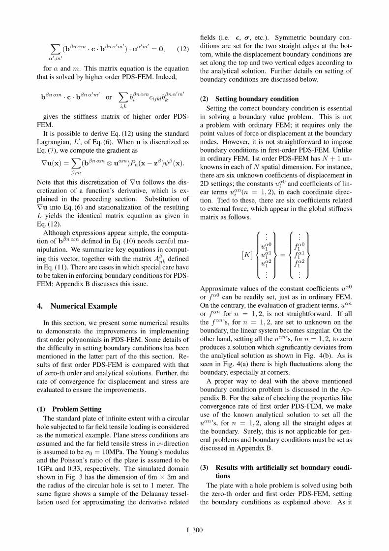
(1) Problem SettingThe standard plate of infinite extent with a circular

hole subjected to far field tensile loading is consideredas the numerical example. Plane stress conditions areassumed and the far field tensile stress in x-directionis assumed to be σ0 = 10MPa. The Young’s modulusand the Poisson’s ratio of the plate is assumed to be1GPa and 0.33, respectively. The simulated domainshown in Fig. 3 has the dimension of 6m × 3m andthe radius of the circular hole is set to 1 meter. Thesame figure shows a sample of the Delaunay tessel-lation used for approximating the derivative related

fields (i.e. ϵ, σ, etc.). Symmetric boundary con-ditions are set for the two straight edges at the bot-tom, while the displacement boundary conditions areset along the top and two vertical edges according tothe analytical solution. Further details on setting ofboundary conditions are discussed below.

(2) Setting boundary conditionSetting the correct boundary condition is essential

in solving a boundary value problem. This is nota problem with ordinary FEM; it requires only thepoint values of force or displacement at the boundarynodes. However, it is not straightforward to imposeboundary conditions in first-order PDS-FEM. Unlikein ordinary FEM, 1st order PDS-FEM has N + 1 un-knowns in each of N spatial dimension. For instance,there are six unknown coefficients of displacement in2D settings; the constants uα0i and coefficients of lin-ear terms uαni (n = 1, 2), in each coordinate direc-tion. Tied to these, there are six coefficients relatedto external force, which appear in the global stiffnessmatrix as follows.

[K]

...uα01uα11uα21

...

=

...fα01

fα11

fα21...

Approximate values of the constant coefficients uα0

or fα0 can be readily set, just as in ordinary FEM.On the contrary, the evaluation of gradient terms, uαn

or fαn for n = 1, 2, is not straightforward. If allthe fαn’s, for n = 1, 2, are set to unknown on theboundary, the linear system becomes singular. On theother hand, setting all the uαn’s, for n = 1, 2, to zeroproduces a solution which significantly deviates fromthe analytical solution as shown in Fig. 4(b). As isseen in Fig. 4(a) there is high fluctuations along theboundary, especially at corners.

A proper way to deal with the above mentionedboundary condition problem is discussed in the Ap-pendix B. For the sake of checking the properties likeconvergence rate of first order PDS-FEM, we makeuse of the known analytical solution to set all theuαn’s, for n = 1, 2, along all the straight edges atthe boundary. Surely, this is not applicable for gen-eral problems and boundary conditions must be set asdiscussed in Appendix B.

(3) Results with artificially set boundary condi-tions

The plate with a hole problem is solved using boththe zero-th order and first order PDS-FEM, settingthe boundary conditions as explained above. As it

I_300

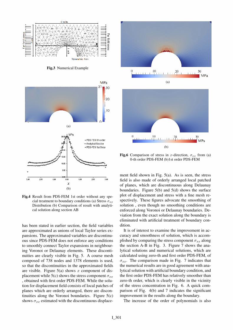
Fig.3 Numerical Example

(a)

(b)

Fig.4 Result from PDS-FEM 1st order without any spe-cial treatment to boundary conditions (a) Stress σxxDistribution (b) Comparison of result with analyti-cal solution along section AB

has been stated in earlier section, the field variablesare approximated as unions of local Taylor series ex-pansions. The approximated variables are discontinu-ous since PDS-FEM does not enforce any conditionsto smoothly connect Taylor expansions in neighbour-ing Voronoi or Delaunay elements. These disconti-nuities are clearly visible in Fig. 5. A course meshcomposed of 738 nodes and 1378 elements is used,so that the discontinuities in the approximated fieldsare visible. Figure 5(a) shows x component of dis-placement while 5(c) shows the stress component σxx, obtained with first order PDS-FEM. While the solu-tion for displacement field consists of local patches ofplanes which are orderly arranged, there are discon-tinuities along the Voronoi boundaries. Figure 5(c)shows σxx estimated with the discontinuous displace-

(a)

(b)

Fig.6 Comparison of stress in x-direction, σxx from (a)0-th order PDS-FEM (b)1st order PDS-FEM

ment field shown in Fig. 5(a). As is seen, the stressfield is also made of orderly arranged local patchedof planes, which are discontinuous along Delaunayboundaries. Figure 5(b) and 5(d) shows the surfaceplot of displacement and stress with a fine mesh re-spectively. These figures advocate the smoothing ofsolution , even though no smoothing conditions areenforced along Voronoi or Delaunay boundaries. De-viation from the exact solution along the boundary iseliminated with artificial treatment of boundary con-dition.

It is of interest to examine the improvement in ac-curacy and smoothness of solution, which is accom-plished by comparing the stress component σxx alongthe section A-B in Fig. 3. Figure 7 shows the ana-lytical solutions and numerical solutions, which arecalculated using zero-th and first order PDS-FEM, ofσxx. The comparison made in Fig. 7 indicates thatthe numerical results are in good agreement with ana-lytical solution with artificial boundary condition, andthe first order PDS-FEM has relatively smoother thanzero-th order, which is clearly visible in the vicinityof the stress concentration in Fig. 6. A quick com-parison of Fig. 4(b) and 7 indicates the significantimprovement in the results along the boundary.

The increase of the order of polynomials is also

I_301

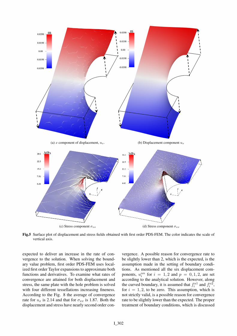
(a) x component of displacement, ux. (b) Displacement component ux

(c) Stress component σxx (d) Stress component σxx

Fig.5 Surface plot of displacement and stress fields obtained with first order PDS-FEM. The color indicates the scale ofvertical axis.

expected to deliver an increase in the rate of con-vergence to the solution. When solving the bound-ary value problem, first order PDS-FEM uses local-ized first order Taylor expansions to approximate bothfunctions and derivatives. To examine what rates ofconvergence are attained for both displacement andstress, the same plate with the hole problem is solvedwith four different tessellations increasing fineness.According to the Fig. 8 the average of convergencerate for ux is 2.14 and that for σxx is 1.87. Both thedisplacement and stress have nearly second order con-

vergence. A possible reason for convergence rate tobe slightly lower than 2, which is the expected, is theassumption made in the setting of boundary condi-tions. As mentioned all the six displacement com-ponents, uαni for i = 1, 2 and p = 0, 1, 2, are setaccording to the analytical solution. However, alongthe curved boundary, it is assumed that fα1i and fα2i ,for i = 1, 2, to be zero. This assumption, which isnot strictly valid, is a possible reason for convergencerate to be slightly lower than the expected. The propertreatment of boundary conditions, which is discussed

I_302

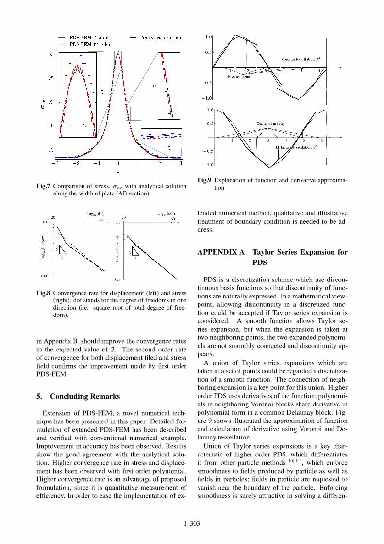
Fig.7 Comparison of stress, σxx with analytical solutionalong the width of plate (AB section)

Fig.8 Convergence rate for displacement (left) and stress(right). dof stands for the degree of freedoms in onedirection (i.e. square root of total degree of free-dom).

in Appendix B, should improve the convergence ratesto the expected value of 2. The second order rateof convergence for both displacement filed and stressfield confirms the improvement made by first orderPDS-FEM.

5. Concluding Remarks

Extension of PDS-FEM, a novel numerical tech-nique has been presented in this paper. Detailed for-mulation of extended PDS-FEM has been describedand verified with conventional numerical example.Improvement in accuracy has been observed. Resultsshow the good agreement with the analytical solu-tion. Higher convergence rate in stress and displace-ment has been observed with first order polynomial.Higher convergence rate is an advantage of proposedformulation, since it is quantitative measurement ofefficiency. In order to ease the implementation of ex-

Fig.9 Explanation of function and derivative approxima-tion

tended numerical method, qualitative and illustrativetreatment of boundary condition is needed to be ad-dress.

APPENDIX A Taylor Series Expansion forPDS

PDS is a discretization scheme which use discon-tinuous basis functions so that discontinuity of func-tions are naturally expressed. In a mathematical view-point, allowing discontinuity in a discretized func-tion could be accepted if Taylor series expansion isconsidered. A smooth function allows Taylor se-ries expansion, but when the expansion is taken attwo neighboring points, the two expanded polynomi-als are not smoothly connected and discontinuity ap-pears.

A union of Taylor series expansions which aretaken at a set of points could be regarded a discretiza-tion of a smooth function. The connection of neigh-boring expansion is a key point for this union. Higherorder PDS uses derivatives of the function; polynomi-als in neighboring Voronoi blocks share derivative inpolynomial form in a common Delaunay block. Fig-ure 9 shows illustrated the approximation of functionand calculation of derivative using Voronoi and De-launay tessellation.

Union of Taylor series expansions is a key char-acteristic of higher order PDS, which differentiatesit from other particle methods 10),11), which enforcesmoothness to fields produced by particle as well asfields in particles; fields in particle are requested tovanish near the boundary of the particle. Enforcingsmoothness is surely attractive in solving a differen-

I_303

tial equation. However, it is contradicting to the con-sequence of the Taylor series expansion, i.e., a smoothfunction allows Taylor series expansion but the ex-panded polynomials cannot be smoothly connected toeach other.

We are not denying the usefulness of the well-established particle methods. Instead, we are pointingout the consequence of Taylor series expansion, andthere could be a room to improve the particle meth-ods. A function discretized by PDS has discontinuityeverywhere, which is a draw back in the viewpointof the particle method. A further study is needed toinvestigate discontinuities of a discretized function.

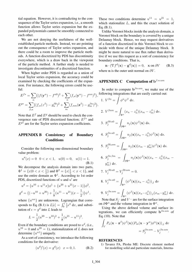
When higher order PDS is regarded as a union oflocal Taylor series expansion, the accuracy could beexamined by checking the coefficients of the expan-sion. For instance, the following errors could be use-ful:

Ef∗ =∑α

((f(yα)− fα0)2 +

∑n

(f,n(yα)− fαn)2

),

Eg∗ =∑β,n

((f,n(z

β)− gβ0n )2 +∑m

(f,nm(zβ)− gβnm )2).

Note thatEf andEg should be used to check the con-vergence rate of PDS discretized function; Ef∗ andEg∗ are for the Taylor series expansion coefficients.

APPENDIX B Consistency of BoundaryConditions

Consider the following one-dimensional boundaryvalue problem:

u′′(x) = 0 0 < x < 1, u(0) = 0, u(1) = 1.(B.1)

We decompose the analysis domain into two parts,Φ1 = x|0 < x < 1

2 and Φ2 = x|12 < x < 1, anduse the entire domain as Ψ1. According to 1st orderPDS, discretized functions of u and u′ are

ud =(u10 + u11x

)ϕ1 +

(u20 + u21(x− 1)

)ϕ2,

gd =((−u10 + u20) +

1

8(u11 − u21)(x− 1

2))ψ1,

where uαn are unknowns. Lagrangian that corre-sponds to Eq. (B.1) is L[ϵ] =

∫ 10

12ϵ

2 dx, and substi-tution of ϵ = gd into L leads to

L =1

2(u20 − u10)2 +

1

8(u21 − u11)2.

Even if the boundary conditions are posed to ud, (i.e.,u10 = 0 and u20 = 1), stationalization of L does notdetermine uα1 uniquely.

As a sort of consistency, we introduce the followingconditions for the derivative:

(ud)′(x) = gd(x) x = 0, 1. (B.2)

These two conditions determine u11 = u21 = 1,which stationalize L, and this the exact solution ofEq. (B.1).

Unlike Voronoi blocks inside the analysis domain, aVoronoi block on the boundary is covered by a uniqueDelaunay block. Hence, we may request derivativesof a function discretized in this Voronoi block to co-incide with those of the unique Delaunay block. Itmight be more natural to use flux rather than deriva-tive if we use this request as a sort of consistency forboundary conditions. That is,

n · (∇fd(x)− gd(x)) = 0, x on ∂V (B.3)where n is the outer unit normal on ∂V .

APPENDIX C Computation of bβ.nαm

In order to compute bβnαm, we make use of thefollowing integrations that are easily carried out:

1. V βα =

∫ϕαψβ dv.

2. V βnm =

∫Φα

(xn − zβn)(xm − zβm) dv.

3. Sβ0α0j =

∫∂Φα

nj(x)ψβ(x) ds.

4. Sβnα0j =

∫∂Φα

nj(x)(xn − zβn)ψβ(x) ds.

5. Sβ0,αmj =

∫∂Φα

nj(x)(xm − yαm)ψβ(x) ds.

6. Sβnβmj =

∫∂Φα

nj(x)ψβ(x)(xn − zβn)(xm −

yαm) dv.

7. V β0α0j = V β0αm

j = 0.

8. V βnα0j =

∫Φα

(ψβ(x)(xn − zβn)),j dv

9. V βnαmj =

∫Φα

(ψβ(x)(xn−zβn)),j(xm−yαm) dv.

Note that S...j and V ... are for the surface integration

on ∂Φα and the volume integration in Φα.Using the above defined volume and surface in-

tegrations, we can efficiently compute bβnαm ofEq. (10). Note that∫

VPn(x− zβ)ψβ(x)(Pm(x− yα)ϕα(x)),j dv

= Sβnαmj − V βnαm

j .

REFERENCES1) Tavarez FA, Plesha ME: Discrete element method

for modelling solid and particulate materials, Interna-

I_304

tional Journal for Numerical Methods in Engineering,70(4), pp 379–404, 2006.

2) Miehe C, Grses E: A robust algorithm forconfigurational-force-driven brittle crack propa-gation with R-adaptive mesh alignment, InternationalJournal for Numerical Methods in Engineering, 72,pp 127–155, 2007.

3) Moes N, Dolbow J, Belytschko T: A finite elementmethod for crack growth without remeshing. Interna-tional Journal for Numerical Methods in Engineering,46(1), pp 131–150, 1999.

4) Oliver J, Huespe AE, Sanchez PJ: A comparativestudy on finite elements for capturing strong discon-tinuities: E-FEM vs X-FEM, Computer Methods inApplied Mechanics and Engineering, 195, pp 4732–4752, 2006.

5) Hansbo A, Hansbo P: A finite element method for thesimulation of strong and weak discontinuities in solidmechanics, Computer Methods in Applied Mechanicsand Engineering, 193, pp 3523–3540, 2004.

6) M.L.L. Wijerathne, Kenji Oguni, Muneo Hori: Nu-merical analysis of growing crack problem using par-ticle discretization scheme, International Journal forNumerical Methods in Engineering, 80, pp 46–73,2009.

7) Muneo Hori, Kenji Oguni, Hide Sakaguchi: Pro-posal of FEM implemented with particle discretiza-tion scheme for analysis of failure phenomena, Jour-nal of Mechanics and Physics of Solids, 53, pp 681–703, 2005.

8) M.L.L. Wijerathne, Muneo Hori, Hide Sakaguchi andKenji Oguni: 3D dynamic simulation of crack prop-agation in extra corporeal shock wave lithotripsy,IOP Conference Series: Materials Science and Engi-neering, 10(1),doi:10.1088/1757-899X/10/1/012120 ,2010.

9) Chen Hao, Wijerathne Lalith, Hori, Muneo andIchimura Tsuyoshi: Stability of dynamic growth oftwo anti-symmetric cracks using PDS-FEM, Journalof Japan Society of Civil Engineering, Ser. A2 (AM)68(1), pp 10–17, 2012.

10) Gingold RA, Monaghan JJ: Smoothed particle hy-drodynamics: theory and application to non-sphericalstars, Monthly Notices of the Royal Astronomical So-ciety, 181, pp 375–389, 1977.

11) Schlangen E, Garboczi EJ: Fracture simulations ofconcrete using lattice models: computational aspects,Engineering Fracture Mechanics, 57(2), pp 319–332,1997.

(Received June 20, 2014)

I_305