Quantum mirrors of log Calabi-Yau surfaces and higher genus curve counting a thesis presented for the degree of Doctor of Philosophy of Imperial College London by Pierrick Bousseau Department of Mathematics Imperial College 180 Queen’s Gate, London SW7 2BZ June 2018

Welcome message from author
This document is posted to help you gain knowledge. Please leave a comment to let me know what you think about it! Share it to your friends and learn new things together.
Transcript

Quantum mirrors of log Calabi-Yausurfaces and higher genus curve counting
a thesis presented for the degree of
Doctor of Philosophy of Imperial College London
by
Pierrick Bousseau
Department of Mathematics
Imperial College
180 Queen’s Gate, London SW7 2BZ
June 2018


I certify that this thesis, and the research to which it refers, are the product of my own work,
and that any ideas or quotations from the work of other people, published or otherwise, are
fully acknowledged in accordance with the standard referencing practices of the discipline.
3

Copyright
The copyright of this thesis rests with the author and is made available under a Creative
Commons Attribution Non-Commercial No Derivatives licence. Researchers are free to copy,
distribute or transmit the thesis on the condition that they attribute it, that they do not
use it for commercial purposes and that they do not alter, transform or build upon it. For
any reuse or redistribution, researchers must make clear to others the licence terms of this
work.
4

Thesis advisor: Professor Richard Thomas Pierrick Bousseau
Quantum mirrors of log Calabi-Yau surfaces and higher genuscurve counting
Abstract
We present three results, at the intersection of tropical geometry, enumerative geometry,
mirror symmetry and non-commutative algebra.
1. A correspondence between Block-Gottsche q-refined tropical curve counting and higher
genus log Gromov-Witten theory of toric surfaces.
2. A correspondence between q-refined two-dimensional Kontsevich-Soibelman scattering
diagrams and higher genus log Gromov-Witten theory of log Calabi-Yau surfaces.
3. A q-deformation of the Gross-Hacking-Keel mirror construction, producing a defor-
mation quantization with canonical basis for the Gross-Hacking-Keel families of log
Calabi-Yau surfaces.
These results are logically dependent: the proof of the third result relies on the second,
whose proof itself relies on the first. Nevertheless, each of them is of independent interest.
5

To my parents.
6

Acknowledgments
I would like to thank my supervisor Richard Thomas for continuous support and innumerous
discussions, suggestions and corrections.
I thank the examiners, Mark Gross and Johannes Nicaise, for careful reading and corrections.
I thank Tom Bridgeland, Michel van Garrel, Lothar Gottsche, Mark Gross, Liana Heuberger,
Ilia Itenberg, Yanki Lekili, Rahul Pandharipande, Bernd Siebert, Jacopo Stoppa for vari-
ous invitations to conferences and seminars, where some results of this thesis have been
presented, and for useful comments and discussions.
I thank Navid Nabijou, Dan Pomerleano and Vivek Shende for specific discussions directly
related to the content of this thesis.
This work would not have been possible without the London mathematical environment and
they are too many people to mention. This includes members and graduate students of the
Departments of Mathematics of Imperial College London, UCL, KCL, and in particular my
fellows of the LSGNT program.
Finally, thanks to all the people met around the world during conferences and having con-
tributed to my mathematical education, and who are again too numerous to list.
This work has been supported by the EPSRC award 1513338, Counting curves in algebraic
geometry, Imperial College London, and has benefited from the EPRSC [EP/L015234/1],
EPSRC Centre for Doctoral Training in Geometry and Number Theory (The London School
of Geometry and Number Theory), University College London.
7


Contents
Introduction 13
Introduction to Chapter 1 . . . . . . . . . . . . . . . . . . . . . . . . . . . . . . . . . . . 13
Introduction to Chapter 2 . . . . . . . . . . . . . . . . . . . . . . . . . . . . . . . . . . . 18
Introduction to Chapter 3 . . . . . . . . . . . . . . . . . . . . . . . . . . . . . . . . . . . 23
1 Tropical refined curve counting from higher genera 27
1.1 Precise statement of the main result . . . . . . . . . . . . . . . . . . . . . . . . . 27
1.1.1 Toric geometry . . . . . . . . . . . . . . . . . . . . . . . . . . . . . . . . . . 27
1.1.2 Log Gromov-Witten invariants . . . . . . . . . . . . . . . . . . . . . . . . 28
1.1.3 Tropical curves . . . . . . . . . . . . . . . . . . . . . . . . . . . . . . . . . . 30
1.1.4 Unrefined correspondence theorem . . . . . . . . . . . . . . . . . . . . . . 33
1.1.5 Refined correspondence theorem . . . . . . . . . . . . . . . . . . . . . . . 33
1.1.6 Fixing points on the toric boundary . . . . . . . . . . . . . . . . . . . . . 35
1.1.7 An explicit example . . . . . . . . . . . . . . . . . . . . . . . . . . . . . . . 36
1.2 Gluing and vanishing properties of lambda classes . . . . . . . . . . . . . . . . . 37
1.3 Toric degeneration and decomposition formula . . . . . . . . . . . . . . . . . . . 38
1.3.1 Tropicalization . . . . . . . . . . . . . . . . . . . . . . . . . . . . . . . . . . 38
1.3.2 Toric degeneration . . . . . . . . . . . . . . . . . . . . . . . . . . . . . . . . 40
1.3.3 Decomposition formula . . . . . . . . . . . . . . . . . . . . . . . . . . . . . 43
1.4 Non-torically transverse stable log maps in X∆ . . . . . . . . . . . . . . . . . . . 46
1.5 Statement of the gluing formula . . . . . . . . . . . . . . . . . . . . . . . . . . . . 49
1.5.1 Preliminaries . . . . . . . . . . . . . . . . . . . . . . . . . . . . . . . . . . . 49
1.5.2 Contribution of trivalent vertices . . . . . . . . . . . . . . . . . . . . . . . 50
1.5.3 Contribution of bivalent pointed vertices . . . . . . . . . . . . . . . . . . 51
1.5.4 Contribution of bivalent unpointed vertices . . . . . . . . . . . . . . . . . 51
1.5.5 Statement of the gluing formula . . . . . . . . . . . . . . . . . . . . . . . 52
1.6 Proof of the gluing formula . . . . . . . . . . . . . . . . . . . . . . . . . . . . . . . 55
1.6.1 Cutting . . . . . . . . . . . . . . . . . . . . . . . . . . . . . . . . . . . . . . 55
1.6.2 Counting log structures . . . . . . . . . . . . . . . . . . . . . . . . . . . . . 58
1.6.3 Comparing obstruction theories . . . . . . . . . . . . . . . . . . . . . . . . 63
9

1.6.4 Gluing . . . . . . . . . . . . . . . . . . . . . . . . . . . . . . . . . . . . . . . 66
1.6.5 Identifying the pieces . . . . . . . . . . . . . . . . . . . . . . . . . . . . . . 68
1.6.6 End of the proof of the gluing formula . . . . . . . . . . . . . . . . . . . . 70
1.7 Vertex contribution . . . . . . . . . . . . . . . . . . . . . . . . . . . . . . . . . . . 71
1.7.1 Reduction to a function of the multiplicity . . . . . . . . . . . . . . . . . 71
1.7.2 Reduction to vertices of multiplicity 1 and 2 . . . . . . . . . . . . . . . . 75
1.7.3 Contribution of vertices of multiplicity 1 and 2 . . . . . . . . . . . . . . 78
1.7.4 Contribution of a general vertex . . . . . . . . . . . . . . . . . . . . . . . 85
1.8 Comparison with known results for K3 and abelian surfaces . . . . . . . . . . . 85
1.8.1 K3 surfaces . . . . . . . . . . . . . . . . . . . . . . . . . . . . . . . . . . . . 86
1.8.2 Abelian surfaces . . . . . . . . . . . . . . . . . . . . . . . . . . . . . . . . . 88
1.9 Descendants and refined broccoli invariants . . . . . . . . . . . . . . . . . . . . . 89
2 The quantum tropical vertex 93
2.1 Scattering . . . . . . . . . . . . . . . . . . . . . . . . . . . . . . . . . . . . . . . . . 93
2.1.1 Torus . . . . . . . . . . . . . . . . . . . . . . . . . . . . . . . . . . . . . . . 93
2.1.2 Quantum torus . . . . . . . . . . . . . . . . . . . . . . . . . . . . . . . . . . 94
2.1.3 Automorphisms of formal families of tori . . . . . . . . . . . . . . . . . . 94
2.1.4 Scattering diagrams . . . . . . . . . . . . . . . . . . . . . . . . . . . . . . . 96
2.2 Gromov-Witten theory of log Calabi-Yau surfaces . . . . . . . . . . . . . . . . . 98
2.2.1 Log Calabi-Yau surfaces . . . . . . . . . . . . . . . . . . . . . . . . . . . . 99
2.2.2 Curve classes . . . . . . . . . . . . . . . . . . . . . . . . . . . . . . . . . . . 99
2.2.3 Log Gromov-Witten invariants . . . . . . . . . . . . . . . . . . . . . . . . 100
2.2.4 3-dimensional interpretation of the invariants NYmg,p . . . . . . . . . . . . 101
2.2.5 Orbifold Gromov-Witten theory . . . . . . . . . . . . . . . . . . . . . . . 103
2.3 Main results . . . . . . . . . . . . . . . . . . . . . . . . . . . . . . . . . . . . . . . . 104
2.3.1 Statement . . . . . . . . . . . . . . . . . . . . . . . . . . . . . . . . . . . . . 104
2.3.2 Examples . . . . . . . . . . . . . . . . . . . . . . . . . . . . . . . . . . . . . 106
2.3.3 Orbifold generalization . . . . . . . . . . . . . . . . . . . . . . . . . . . . . 108
2.3.4 More general quantum scattering diagrams . . . . . . . . . . . . . . . . . 109
2.4 Gromov-Witten theory of toric surfaces . . . . . . . . . . . . . . . . . . . . . . . 110
2.4.1 Curve classes on toric surfaces . . . . . . . . . . . . . . . . . . . . . . . . 110
2.4.2 Log Gromov-Witten invariant of toric surfaces . . . . . . . . . . . . . . . 111
2.5 Degeneration from log Calabi-Yau to toric . . . . . . . . . . . . . . . . . . . . . . 112
10

2.5.1 Degeneration formula: statement . . . . . . . . . . . . . . . . . . . . . . . 112
2.5.2 Degeneration set-up . . . . . . . . . . . . . . . . . . . . . . . . . . . . . . . 113
2.5.3 Statement of the decomposition formula . . . . . . . . . . . . . . . . . . 115
2.5.4 Classification of rigid tropical curves . . . . . . . . . . . . . . . . . . . . . 118
2.5.5 Gluing formula . . . . . . . . . . . . . . . . . . . . . . . . . . . . . . . . . . 122
2.5.6 End of the proof of the degeneration formula . . . . . . . . . . . . . . . . 126
2.6 Scattering and tropical curves . . . . . . . . . . . . . . . . . . . . . . . . . . . . . 127
2.6.1 Refined tropical curve counting . . . . . . . . . . . . . . . . . . . . . . . . 128
2.6.2 Elementary quantum scattering . . . . . . . . . . . . . . . . . . . . . . . . 129
2.6.3 Quantum scattering from refined tropical curve counting . . . . . . . . 130
2.7 End of the proof of Theorems 2.6 and 2.7 . . . . . . . . . . . . . . . . . . . . . . 134
2.7.1 End of the proof of Theorem 2.6 . . . . . . . . . . . . . . . . . . . . . . . 134
2.7.2 End of the proof of Theorem 2.7 . . . . . . . . . . . . . . . . . . . . . . . 135
2.8 Integrality results and conjectures . . . . . . . . . . . . . . . . . . . . . . . . . . . 139
2.8.1 Integrality conjecture . . . . . . . . . . . . . . . . . . . . . . . . . . . . . . 139
2.8.2 Integrality result . . . . . . . . . . . . . . . . . . . . . . . . . . . . . . . . . 141
2.8.3 Quadratic refinement . . . . . . . . . . . . . . . . . . . . . . . . . . . . . . 142
2.8.4 Proof of the integrality theorem . . . . . . . . . . . . . . . . . . . . . . . 145
2.8.5 Integrality and quiver DT invariants . . . . . . . . . . . . . . . . . . . . . 147
2.8.6 del Pezzo surfaces . . . . . . . . . . . . . . . . . . . . . . . . . . . . . . . . 150
2.9 Relation with Cecotti-Vafa . . . . . . . . . . . . . . . . . . . . . . . . . . . . . . . 152
2.9.1 Summary of the Cecotti-Vafa argument . . . . . . . . . . . . . . . . . . . 152
2.9.2 Comparison with Theorem 2.6 . . . . . . . . . . . . . . . . . . . . . . . . 154
2.9.3 Ooguri-Vafa integrality . . . . . . . . . . . . . . . . . . . . . . . . . . . . . 154
3 Deformation quantization of log Calabi-Yau surfaces 156
3.1 Basics and main results . . . . . . . . . . . . . . . . . . . . . . . . . . . . . . . . . 156
3.1.1 Looijenga pairs . . . . . . . . . . . . . . . . . . . . . . . . . . . . . . . . . . 156
3.1.2 Tropicalization of Looijenga pairs . . . . . . . . . . . . . . . . . . . . . . 158
3.1.3 Algebras and quantum algebras . . . . . . . . . . . . . . . . . . . . . . . . 159
3.1.4 Ore localization . . . . . . . . . . . . . . . . . . . . . . . . . . . . . . . . . 160
3.1.5 The Gross-Hacking-Keel mirror family . . . . . . . . . . . . . . . . . . . 161
3.1.6 Deformation quantization . . . . . . . . . . . . . . . . . . . . . . . . . . . 162
3.1.7 Main results . . . . . . . . . . . . . . . . . . . . . . . . . . . . . . . . . . . 163
11

3.2 Quantum modified Mumford degenerations . . . . . . . . . . . . . . . . . . . . . 165
3.2.1 Building blocks . . . . . . . . . . . . . . . . . . . . . . . . . . . . . . . . . 165
3.2.2 Quantum scattering diagrams . . . . . . . . . . . . . . . . . . . . . . . . . 169
3.2.3 Quantum automorphisms . . . . . . . . . . . . . . . . . . . . . . . . . . . 171
3.2.4 Gluing . . . . . . . . . . . . . . . . . . . . . . . . . . . . . . . . . . . . . . . 173
3.2.5 Result of the gluing for I = J . . . . . . . . . . . . . . . . . . . . . . . . . . 175
3.2.6 Quantum broken lines and theta functions . . . . . . . . . . . . . . . . . 176
3.2.7 Deformation quantization of the mirror family . . . . . . . . . . . . . . . 178
3.2.8 The algebra structure . . . . . . . . . . . . . . . . . . . . . . . . . . . . . . 180
3.3 The canonical quantum scattering diagram . . . . . . . . . . . . . . . . . . . . . 182
3.3.1 Log Gromov-Witten invariants . . . . . . . . . . . . . . . . . . . . . . . . 182
3.3.2 Definition . . . . . . . . . . . . . . . . . . . . . . . . . . . . . . . . . . . . . 183
3.3.3 Consistency . . . . . . . . . . . . . . . . . . . . . . . . . . . . . . . . . . . . 184
3.3.4 Reduction to the Gross-Siebert locus. . . . . . . . . . . . . . . . . . . . . 185
3.3.5 Pushing the singularities at infinity . . . . . . . . . . . . . . . . . . . . . 187
3.3.6 Consistency of ν(Dcan) . . . . . . . . . . . . . . . . . . . . . . . . . . . . . 188
3.3.7 Comparing Dcan and ν(Dcan) . . . . . . . . . . . . . . . . . . . . . . . . . 190
3.3.8 End of the proof of Theorem 3.26 . . . . . . . . . . . . . . . . . . . . . . 192
3.4 Extension over boundary strata . . . . . . . . . . . . . . . . . . . . . . . . . . . . 193
3.4.1 Torus equivariance . . . . . . . . . . . . . . . . . . . . . . . . . . . . . . . 193
3.4.2 End of the proof of Theorem 3.7 . . . . . . . . . . . . . . . . . . . . . . . 194
3.4.3 Quantization of V1 and V2 . . . . . . . . . . . . . . . . . . . . . . . . . . 195
3.4.4 End of the proof of Theorem 3.8 . . . . . . . . . . . . . . . . . . . . . . . 199
3.4.5 q-integrality: end of the proof of Theorem 3.9 . . . . . . . . . . . . . . . 200
3.5 Example: degree 5 del Pezzo surfaces . . . . . . . . . . . . . . . . . . . . . . . . . 202
3.6 Higher genus mirror symmetry and string theory . . . . . . . . . . . . . . . . . . 203
3.6.1 From higher genus to quantization via Chern-Simons . . . . . . . . . . . 203
3.6.2 Quantization and higher genus mirror symmetry . . . . . . . . . . . . . 204
Bibliography 206
12

Introduction
In this thesis, we present some contributions at the intersection of tropical geometry, enu-
merative geometry, mirror symmetry and non-commutative algebra. The text is divided in
three chapters.
Chapter 1 is about enumerative geometry, more precisely log Gromov-Witten invariants, of
complex toric surfaces, and tropical geometry of the real plane. We solve the all genus log
Gromov-Witten theory, with insertion of the top lambda class, of toric surfaces. The answer
is formulated in terms of q-refined counts of tropical curves and conversely gives a previously
unknown geometric meaning to these q-refined counts.
Chapter 2 is about enumerative geometry, more precisely log Gromov-Witten invariants, of
log Calabi-Yau surfaces with maximal boundary, i.e. of pairs (Y,D), where Y is a smooth
projective complex surface and D is a singular reduced normal crossing effective anticanon-
ical divisor. The class of log Calabi-Yau surfaces is a natural extension of the class of toric
surfaces. In particular, the complement U = Y −D is a non-compact algebraic symplectic
surface, generalization of (C∗)2, and non-compact analogue of K3 surfaces. We solve the all
genus log Gromov-Witten theory, with insertion of the top lambda class, of log Calabi-Yau
surfaces. The answer is formulated in terms of algebraic and combinatorial objects: q-refined
scattering diagrams. The proof is done by reduction to the toric case, for which the main
result of Chapter 1 is used.
Chapter 3 is about deformation quantization of log Calabi-Yau surfaces. Using the log
Gromov-Witten invariants studied in Chapter 2 as input, we construct non-commutative
algebras, deformation quantizations of Poisson algebras of regular functions on the non-
compact surfaces U . It seems to be a new way to construct non-commutative algebras.
The genus zero/unrefined/commutative versions of these results were previously known.
More precisely, our Chapters 1-2-3 can be viewed as a higher genus/q-refined/non-commutative
generalization of the series of papers [Mik05][NS06]-[GPS10]-[GHK15a].
We give below detailed Introductions to each of the three Chapters.
Introduction to Chapter 1
Tropical geometry gives a combinatorial way to approach problems in complex and real al-
gebraic geometry. An early success of this approach is Mikhalkin’s correspondence theorem
[Mik05], proved differently and generalized by Nishinou and Siebert [NS06], between counts
of complex algebraic curves in complex toric surfaces and counts with multiplicity of tropical
curves in R2. The main result of Chapter 1, Theorem 1, is an extension to a correspon-
dence between some generating series of higher genus log Gromov-Witten invariants of toric
13

surfaces and counts with q-multiplicity of tropical curves in R2.
Counts of tropical curves in R2 with q-multiplicity were introduced by Block and Gottsche
[BG16]. The usual multiplicity of a tropical curve is defined as a product of integer mul-
tiplicities attached to the vertices. Block and Gottsche remarked that one can obtain a
refinement by replacing the multiplicity m of a vertex by its q-analogue
[m]q ∶=qm2 − q−
m2
q12 − q−
12
= q−m−1
2 (1 + q + ⋅ ⋅ ⋅ + qm−1) .
The q-multiplicity of a tropical curve is then the product of the q-multiplicities of the vertices.
The count with q-multiplicity of tropical curves specializes for q = 1 to the ordinary count
with multiplicity. This definition is done at the tropical level so is combinatorial in nature
and its geometric meaning is a priori unclear.
Let ∆ be a balanced collection of vectors in Z2 and let n be a non-negative integer1. This
determines a complex toric surface X∆ and a counting problem of virtual dimension zero
for complex algebraic curves in X∆ of some genus g∆,n, of some class β∆, satisfying some
tangency conditions with respect to the toric boundary divisor, and passing through n points
of X∆ in general position. Let N∆,n ∈ N be the solution to this counting problem. According
to Mikhalkin’s correspondence theorem, N∆,n is a count with multiplicity of tropical curves
in R2, and so it has a Block-Gottsche refinement N∆,n(q) ∈ N[q±12 ].
For every g ⩾ g∆,n, we consider the same counting problem as before—same curve class,
same tangency conditions—but for curves of genus g. The virtual dimension is now g−g∆,n.
To obtain a number, we integrate a class of degree g − g∆,n, the lambda class λg−g∆,n, over
the virtual fundamental class of a corresponding moduli space of stable log maps. For every
g ⩾ g∆,n, we get a log Gromov-Witten invariant N∆,ng ∈ Q.
Theorem 1. For every ∆ balanced collection of vectors in Z2, and for every non-negative
integer n such that g∆,n ⩾ 0, we have the equality
∑g⩾g∆,n
N∆,ng u2g−2+∣∆∣
= N∆,n(q) ((−i)(q
12 − q−
12 ))
2g∆,n−2+∣∆∣
of power series in u with rational coefficients, where
q = eiu = ∑n⩾0
(iu)n
n!,
and ∣∆∣ is the cardinality of ∆.
Remarks
• According to Theorem 1, the knowledge of the Block-Gottsche invariant N∆,n(q) is
equivalent to the knowledge of the log Gromov-Witten invariants N∆,ng for all g ⩾ g∆,n.
This provides a geometric meaning to Block-Gottsche invariants, independent of any
choice of tropical limit, making their deformation invariance manifest.
1Precise definitions are given in Section 1.1.
14

• Given a family π∶C → B of nodal curves, the Hodge bundle E is the rank g vector bundle
over B whose fiber over b ∈ B is the space H0(Cb, ωCb) of sections of the dualizing
sheaf ωCb of the curve Cb = π−1(b). The lambda classes are classically [Mum83] the
Chern classes of the Hodge bundle:
λj ∶= cj(E) .
The log Gromov-Witten invariantsN∆,ng are defined by an insertion of (−1)g−g∆,nλg−g∆,n
to cut down the virtual dimension from g − g∆,n to zero.
• One can interpret Theorem 1 as establishing integrality and positivity properties for
higher genus log Gromov-Witten invariants of X∆ with one lambda class inserted.
• The change of variables q = eiu makes the correspondence of Theorem 1 quite non-
trivial. In particular, it cannot be reduced to an easy enumerative correspondence. It
is essential to have a virtual/non-enumerative count on the Gromov-Witten side: for
g large enough, most of the contributions to N∆,ng come from maps with contracted
components.
• In Theorem 1.5, we present a generalization of Theorem 1 where some intersection
points with the toric boundary divisor can be fixed.
• One could ask for a generalization of Theorem 1 including descendant log Gromov-
Witten invariants, i.e. with insertion of psi classes. In the simplest case of a trivalent
vertex with insertion of one psi class, we will show in Section 1.9 that it is possible
to reproduce the numerator qm2 + q−
m2 of the multiplicity introduced by Gottsche and
Schroeter [GS16a] in the context of refined broccoli invariants, in a way similar to how
we reproduce the numerator qm2 −q−
m2 of the Block-Gottsche multiplicity in Theorem 1.
Relation with previous works
q-analogues
It is a general principle in mathematics, going back at least to Heine’s introduction of q-
hypergeometric series in 1846, that many “classical” notions have a q-analogue, recovering
the classical one in the limit q → 1. The Block-Gottsche refinement of the tropical curve
counts in R2 is clearly an example of this principle. In many other examples, it is well known
that it is a good idea to write q = eh, the limit q → 1 becoming the limit h → 0. From this
point of view, the change of variable q = eiu in Theorem 1 is maybe not so surprising.
Gottsche-Shende refinement by Hirzebruch genus
Whereas the specialization of Block-Gottsche invariants at q = 1 recovers a count of complex
algebraic curves, the specialization q = −1 recovers in some cases a count of real algebraic
curves in the sense of Welschinger [Wel05]. This strongly suggests a motivic interpretation
of the Block-Gottsche invariants and indeed one of the original motivations of Block and
15

Gottsche was the fact that, under some ampleness assumptions, the refined tropical curve
counts should coincide with the refined curve counts on toric surfaces defined by Gottsche and
Shende [GS14] in terms of Hirzebruch genera of Hilbert schemes. Using motivic integration,
Nicaise, Payne and Schroeter [NPS16] have reduced this conjecture to a conjecture about the
motivic measure of a semialgebraic piece of the Hilbert scheme attached to a given tropical
curve.
Our approach to the Block-Gottsche refined tropical curve counting is clearly different from
the Gottsche-Shende approach: we interpret the refined variable q as coming from the
resummation of a genus expansion whereas they interpret it as a formal parameter keeping
track of the refinement from some Euler characteristic to some Hirzebruch genus.
The Gottsche-Shende refinement makes sense for surfaces more general than toric ones,
as do the higher genus log Gromov-Witten invariants with one lambda class inserted. So
one might ask if Theorem 1 can be extended to more general surfaces, as a relation between
Gottsche-Shende refined invariants and generating series of higher genus log Gromov-Witten
invariants. In Theorem 1.29 and 1.32, we show by combining known results that this is
indeed the case for K3 and abelian surfaces. In particular, Theorem 1 is not an isolated
fact but part of a family of similar results. The case of a log Calabi-Yau surface obtained as
complement of a smooth anticanonical divisor in a del Pezzo surface, and its relation with,
in physics terminology, a worldsheet definition of the refined topological string of local del
Pezzo 3-folds, will be discussed in a future work.
MNOP
The change of variables q = eiu is reminiscent of the MNOP, [MNOP06a], [MNOP06b],
Gromov-Witten/ Donaldson-Thomas (DT) correspondence on 3-folds. The log Gromov-
Witten invariants N∆,ng can be rewritten as C∗-equivariant log Gromov-Witten invariants
of the 3-fold X∆×C, where C∗ acts by scaling on C, see Lemma 7 of Maulik-Pandharipande-
Thomas [MPT10]. If a log DT theory and a log MNOP correspondence were developed, this
would predict that the generating series of N∆,ng is a rational function in q = eiu, which is
indeed true by Theorem 1. But it would not be enough to imply Theorem 1 because the
relation between log DT invariants and Block-Gottsche invariants is a priori unclear. In
fact, the Gottsche-Shende conjecture and the result of Filippini and Stoppa suggest that
Block-Gottsche invariants are refined DT invariants whereas the MNOP correspondence
involves unrefined DT invariants. This topic will be discussed in more details elsewhere.
BPS integrality
When the log Gromov-Witten invariants of X∆ ×C coincide with ordinary Gromov-Witten
invariants of X∆ × C, which is probably the case if ∣v∣ = 1 for every v ∈ ∆ and if the
toric boundary divisor of X∆ is positive enough, then the integrality implied by Theorem 1
coincides with the BPS integrality predicted by Pandharipande [Pan99], and proved via
symplectic methods by Zinger [Zin11], for generating series of Gromov-Witten invariants of
a 3-fold and of curve class intersecting positively the anticanonical divisor.
16

Mikhalkin refined real count
Mikhalkin [Mik15] has given an interpretation of some particular Block-Gottsche invariants
in terms of counts of real curves. We do not understand the relation with our approach in
terms of higher genus log Gromov-Witten invariants. We merely remark that both for us
and for Mikhalkin, it is the numerator of the Block-Gottsche multiplicities which appears
naturally.
Parker theory of exploded manifolds
This Chapter owes a great intellectual debt towards the paper [Par16] of Brett Parker,
where a correspondence theorem between tropical curves in R3 and some generating series
of curve counts in exploded versions of toric 3-folds is proved. Indeed, a conjectural version of
Theorem 1 was known to the author around April 20162 but it was only after the appearance
of [Par16] in August 2016 that it became clear that this result should be provable with
existing technology. In particular, the idea to reduce the amount of explicit computations
by exploiting the consistency of some gluing formula (see Section 1.7) follows [Par16].
Plan of Chapter 1
In Section 1.1, we fix our notations and we describe precisely the objects involved in the
formulation of Theorem 1. In Section 1.2, we review some gluing and vanishing properties
of the lambda classes.
The next five Sections form the proof of Theorem 1.
The first step of the proof, described in Section 1.3, is an application of the decomposition
formula of Abramovich, Chen, Gross and Siebert [ACGS17a] to the toric degeneration of
Nishinou, Siebert [NS06]. This gives a way to write our log Gromov-Witten invariants as a
sum of contributions indexed by tropical curves.
In the second step of the proof, described in Sections 1.5 and 1.6, we prove a gluing formula
which gives a way to write the contribution of a tropical curve as a product of contributions
of its vertices. Here, gluing and vanishing properties of the lambda classes reviewed in
Section 1.2, combined with a structure result for non-torically transverse stable log maps
proved in Section 1.4, play an essential role. In particular, we only have to glue torically
transverse stable log maps and we don’t need to worry about the technical issues making
the general gluing formula in log Gromov-Witten theory difficult (see Abramovich, Chen,
Gross, Siebert [ACGS17b]).
After the decomposition and gluing steps, what remains to do is to compute the contribution
to the log Gromov-Witten invariants of a tropical curve with a single trivalent vertex. The
third and final step of the proof of Theorem 1, carried out in Section 1.7, is the explicit
evaluation of this vertex contribution. Consistency of the gluing formula leads to non-trivial
2And was for example presented at the Workshop: Curves on surfaces and 3-folds, EPFL, Lausanne, 21June 2016.
17
relations between these vertex contributions, which enable us to reduce the problem to
particularly simple vertices. The contribution of these simple vertices is computed explicitly
by reduction to Hodge integrals previously computed by Bryan and Pandharipande [BP05]
and this ends the proof of Theorem 1.
In Section 1.8, we prove Theorem 1.29 and Theorem 1.32, which are analogues for K3 and
abelian surfaces of Theorem 1 for toric surfaces.
In Section 1.9, we make contact in a simple case with refined broccoli invariants.
Introduction to Chapter 2
Statements
We start by giving slightly imprecise versions of the main results of this Chapter. For us,
a log Calabi-Yau surface is a pair (Y,D), where Y is a smooth complex projective surface
and D is a reduced effective normal crossing anticanonical divisor on Y . A log Calabi-Yau
surface (Y,D) has maximal boundary3 if D is singular.
Theorem 2. The functions attached to the rays of the q-deformed 2-dimensional Kontsevich-
Soibelman scattering diagrams are, after the change of variables q = eih, generating series of
higher genus log Gromov-Witten invariants—with maximal tangency condition and insertion
of the top lambda class—of log Calabi-Yau surfaces with maximal boundary.
A precise version of Theorem 2 is given by Theorems 2.6 and 2.7 in Section 2.3.
Theorem 3. Higher genus log Gromov-Witten invariants–with maximal tangency condition
and insertion of the top lambda class–of log Calabi-Yau surfaces with maximal boundary
satisfy an Ooguri-Vafa/open BPS integrality property.
A precise version of Theorem 3 is given by Theorem 2.30 in Section 2.8.
We also formulate a new conjecture.
Conjecture 4. Higher genus relative Gromov-Witten invariants-with maximal tangency
condition and insertion of the top lambda class–of a del Pezzo surface S relatively to a
smooth anticanonical divisor are related to refined counts of dimension one stable sheaves
on the local Calabi-Yau 3-fold TotKS, total space of the canonical line bundle of S.
A precise version of Conjecture 4 is given by Conjecture 2.41 in Section 2.8.6.
3In Chapter 3, following [GHK15a], a log Calabi-Yau surface with maximal boundary is called a Looijengapair.
18

Context and motivations
SYZ
The Strominger-Yau-Zaslow [SYZ96] picture of mirror symmetry suggests a two steps con-
struction of the mirror of a Calabi-Yau variety admitting a Lagrangian torus fibration: first,
construct the “semi-flat” mirror by dualizing the non-singular torus fibers; second, correct
the complex structure of the “semi-flat” mirror such that it extends across the locus of singu-
lar fibers. It is expected, [SYZ96], [Fuk05], that the corrections involved in the second step
are determined by some counts of holomorphic discs in the original variety with boundary
on torus fibers.
KS
In dimensional two and with at most nodal singular fibers in the torus fibration, Kontsevich-
Soibelman [KS06] had the insight that algebraic self-consistency constraints on the correc-
tions were strong enough to determine these corrections uniquely. More precisely, they
reduced the problem to an algebraic computation of commutators in a group of formal
families of symplectomorphisms of the dimension two algebraic torus.
This algebraic formalism, graphically encoded under the form of scattering diagrams, was
generalized and extended to higher dimensions by Gross-Siebert [GS11] and plays an essential
role in the Gross-Siebert algebraic approach to mirror symmetry.
GPS
In [GPS10], Gross-Pandharipande-Siebert made some progress in connecting the original
enumerative expectation and the algebraic recipe of scattering diagrams. They showed
that the 2-dimensional Kontsevich-Soibelman scattering diagrams indeed have an enumer-
ative meaning: they compute some genus zero log Gromov-Witten invariants of some log
Calabi-Yau surfaces with maximal boundary, i.e. complements of a singular normal crossing
anticanonical divisor in a smooth projective surface.
This agrees with the original expectation because these geometries admit Lagrangian torus
fibrations and these genus zero log Gromov-Witten invariants should be thought as algebraic
definitions of some counts of holomorphic discs with boundary on Lagrangian torus fibers4.
The combination of 2-dimensional scattering diagrams with their enumerative interpretation
given by [GPS10] was the main tool in the Gross-Hacking-Keel [GHK15a] construction of
mirrors for log Calabi-Yau surfaces with maximal boundary.
4For some symplectic approach, relating counts of holomorphic discs in hyperkahler manifolds of realdimension 4 and the Konstevich-Soibelman wall-crossing formula, we refer to the works of Lin [Lin17] andIacovino [Iac17].
19

Higher genus GPS = refined KS
At the end of their paper, Section 11.8 of [KS06] (see also [Soi09]), Kontsevich-Soibelman
already remarked that the 2-dimensional scattering diagram formalism has a natural q-
deformation, with the group of formal families of symplectomorphisms of the 2-dimensional
algebraic torus replaced by a group a formal families of automorphisms of the 2-dimensional
quantum torus, a natural non-commutative deformation of the 2-dimensional algebraic torus.
The enumerative meaning of this q-deformed scattering diagram was a priori unclear.
In Section 5.8 of [GPS10], Gross-Pandharipande-Siebert remarked that the genus zero log
Gromov-Witten invariants they consider have a natural extension to higher genus, by inte-
gration of the top lambda class, and they asked if there is an interpretation of these higher
genus invariants in terms of scattering diagrams.
The main result of the present Chapter, Theorem 2, is that the two previous questions, the
enumerative meaning of the algebraic q-deformation and the algebraic meaning of the higher
genus deformation, are answers to each other.
OV
The higher genus log Gromov-Witten invariants of log Calabi-Yau surfaces that we are
considering–with insertion of the top lambda class–should be thought as an algebro-geometric
definition of some counts of higher genus Riemann surfaces with boundary on a Lagrangian
torus fiber in a Calabi-Yau 3-fold geometry, essentially the product of the log Calabi-Yau
surface by a third trivial direction, see Section 2.2.4. For such counts of higher genus open
curves in a Calabi-Yau 3-fold geometry, Ooguri-Vafa [OV00] have conjectured an open BPS
integrality structure. Theorem 3, which is a consequence of Theorem 2 and of non-trivial
algebraic properties of q-deformed scattering diagrams, can be viewed as a check of this BPS
integrality structure.
DT
The non-trivial integrality properties of q-deformed scattering diagrams are well-known to
be related to integrality properties of refined Donaldson-Thomas (DT) invariants, [KS08].
Indeed, q-deformed scattering diagrams control the wall-crossing behavior of refined DT
invariants.
The fact that the integrality structure of DT invariants coincides with the Ooguri-Vafa
integrality structure of higher genus open Gromov-Witten invariants of Calabi-Yau 3-folds,
essentially involving the quantum dilogarithm in both cases, can be viewed as an early
indication that something like Theorem 2 should be true.
As consequence of Theorem 2, we get explicit relations between refined DT invariants of
some quivers and higher genus log Gromov-Witten invariants of log Calabi-Yau surfaces, see
Section 2.8.5, generalizing the unrefined/genus zero relation of [GP10], [RW13].
20

CV
In fact, Cecotti-Vafa [CV09] have given a physical derivation of the wall-crossing formula in
DT theory going through the higher genus open Gromov-Witten theory of some Calabi-Yau
3-fold. We will explain in Section 2.9 that Theorem 2 and 3 are indeed fully compatible with
the Cecotti-Vafa argument. In particular, Theorem 2 can be viewed as a highly non-trivial
mathematical check of the connection predicted by Witten [Wit95] between higher genus
open A-model and quantum Chern-Simons theory.
del Pezzo
Theorem 2 and 3 are about log Calabi-Yau surfaces with maximal boundary, i.e. with a
singular normal crossing anticanonical divisor. Similar questions can be asked for log Calabi-
Yau surfaces with respect to a smooth anticanonical divisor. Conjecture 4 gives a non-trivial
correspondence in such case, suggested by the similarities between refined DT theory and
open higher genus Gromov-Witten invariants discussed above.
Comments on the proof of Theorem 2
The curve counting invariants appearing in Theorem 2 are log Gromov-Witten invariants,
as defined by Gross and Siebert [GS13], and Abramovich and Chen [Che14b], [AC14]. The
proof of Theorem 2 relies on recently developed general properties of log Gromov-Witten
invariants, such as the decomposition formula of [ACGS17a].
The main tool of [GPS10] is a reduction to a tropical setting using the correspondence
theorem of Mikhalkin [Mik05] and Nishinou-Siebert [NS06] between counts of curves in
complex toric surfaces and counts of tropical curves in R2. Similarly, the main tool of the
present Chapter is a reduction to a tropical setting using the main result, Theorem 1, of
Chapter 1.
Given the fact that the relation between q-deformed tropical invariants and q-deformed
scattering diagrams has already been worked out by Filippini-Stoppa [FS15], Theorem 2
should really be viewed as a combination of Theorem 1 and [FS15]. The new results required
for the proof of Theorem 2 are: the check that the degeneration step used in [GPS10] to go
from a log Calabi-Yau setting to a toric setting extends to the higher genus case and the
check that the correspondence given by Theorem 1 has exactly the correct form to be used
as input in [FS15].
The most technical part is the higher genus version of the degeneration step. As the gen-
eral version of the degeneration formula in log Gromov-Witten theory is not yet known,
we combine the general decomposition formula of [ACGS17a] with some situation specific
vanishing statements, which, as in Chapter 1, reduce the gluing operations to some torically
transverse locus where they are under control, for example thanks to [KLR18].
21

Comments on the proof of Theorem 3.
The proof of Theorem 3 is a combination of Theorem 2 and of the non-trivial integral-
ity results about q-deformed scattering diagrams proved by Kontsevich and Soibelman in
Section 6 of [KS11]. In fact, to get the most general form of Theorem 3, the results contained
in [KS11] do not seem to be enough. We use an induction argument on scattering diagrams,
parallel to the one used in Appendix C3 of [GHKK18], to reduce the most general case to a
case which can be treated by [KS11].
A small technical point is to keep track of signs, because of the difference between quantum
tori and twisted quantum tori, see Section 2.8.3 on the quadratic refinement for details.
Plan of Chapter 2
In Section 2.1, we review the notion of 2-dimensional scattering diagrams, both classical
and quantum, with an emphasis on the symplectic/Hamiltonian aspects. In Section 2.2, we
introduce a class of log Calabi-Yau surfaces and their log Gromov-Witten invariants.
In Section 2.3, we state our main result, Theorem 2.6, precise version of Theorem 2, relat-
ing 2-dimensional quantum scattering diagrams and generating series of higher genus log
Gromov-Witten invariants of log Calabi-Yau surfaces. We also state a generalization of
Theorem 2.6, Theorem 2.7, phrased in terms of orbifold log Gromov-Witten invariants.
Sections 2.4, 2.5, 2.6, 2.7 are dedicated to the proof of Theorems 2.6 and 2.7. The general
structure of the proof is parallel to [GPS10]. In Section 2.4, we introduce higher genus
log Gromov-Witten invariants of toric surfaces. In Section 2.5, the most technical part
of this Chapter, we prove a degeneration formula relating log Gromov-Witten invariants
of log Calabi-Yau surfaces defined in Section 2.2 and appearing in Theorem 2.6, with log
Gromov-Witten invariants of toric surfaces defined in Section 2.4.2. In Section 2.6, following
Filippini-Stoppa [FS15], we review the connection between quantum scattering diagrams
and refined counts of tropical curves. We finish the proof of Theorem 2.6 in Section 2.7,
combining the results of Sections 2.5 and 2.6 with Theorem 1. The orbifold Gromov-Witten
computation needed to finish the proof of Theorem 2.7 is done in Section 2.7.2.
In Section 2.8.1, we formulate a BPS integrality conjecture for higher genus log Gromov-
Witten invariants of log Calabi-Yau surfaces. In Section 2.8.2, we state Theorem 2.30, precise
form of Theorem 3. The proof of Theorem 2.30 takes Sections 2.8.3, 2.8.4. In Section 2.8.5,
Theorem 2.38 gives an explicit connection with refined DT invariants of quivers. Finally, in
Section 2.8.6, we state Conjecture 2.41, precise version of Conjecture 4.
In Section 2.9, we explain how Theorem 2 can be viewed as a mathematical check of the
physics work of Cecotti-Vafa [CV09] and how Theorem 3 is compatible with the Ooguri-Vafa
integrality conjecture [OV00].
22

Introduction to Chapter 3
Context and motivations
Mirror symmetry
The Strominger-Yau-Zaslow [SYZ96] picture of mirror symmetry suggests an original way of
constructing algebraic varieties: given a Calabi-Yau variety, its mirror geometry should be
constructed in terms of the enumerative geometry of holomorphic discs in the original variety.
This picture has been developed by Fukaya [Fuk05], Kontsevich-Soibelman [KS06], Gross-
Siebert [GS11], Auroux [Aur07] and many others. In particular, Gross and Siebert have
developed an algebraic approach in which the enumerative geometry of holomorphic discs is
replaced by some genus zero log Gromov-Witten invariants. Given the recent progress in log
Gromov-Witten theory, in particular the definition of punctured invariants by Abramovich-
Chen-Gross-Siebert [ACGS17b], it is likely that this approach will lead to some general
mirror symmetry construction in the algebraic setting, see Gross-Siebert [GS16b] for an
announcement.
The work of Gross-Hacking-Keel
An early version of this mirror construction has been used by Gross-Hacking-Keel [GHK15a]
to construct mirror families of log Calabi-Yau surfaces, with non-trivial applications to the
theory of surface singularities and in particular a proof of the Looijenga’s conjecture on
smoothing of cusp singularities. More precisely, the construction of [GHK15a] applies to
Looijenga pairs, i.e. to pairs (Y,D), where Y is a smooth projective complex surface and
D is some reduced effective normal crossing anticanonical divisor on Y . The upshot is in
general a formal flat family X → S of surfaces over a formal completion, near some point s0,
the “large volume limit of Y”, of an algebraic approximation to a compactification of the
complexified Kahler cone of Y .
Furthermore, X is an affine Poisson formal variety with a canonical linear basis of so-called
theta functions and the map X → S is Poisson if S is equipped with the zero Poisson
bracket. Under some positivity assumptions on (Y,D), this family can be in fact extended
to an algebraic family over an algebraic base and the generic fiber is then a smooth algebraic
symplectic surface.
The first step of the construction involves defining the fiber Xs0 , i.e. the “large complex
structure limit” of the family X . This step is essentially combinatorial and can be reduced
to some toric geometry: Xs0 is a reducible union of toric varieties.
The second step is to construct X by smoothing of Xs0 . This construction is based on the
consideration of an algebraic object, a scattering diagram, notion introduced by Kontsevich-
Soibelman [KS06] and further developed by Gross-Siebert [GS11], whose definition encodes
genus zero log Gromov-Witten invariants5 of (Y,D). The key non-trivial property to check
5In fact, in [GHK15a], an ad hoc definition of genus zero Gromov-Witten invariants is used,which wassupposed to coincide with genus zero log Gromov-Witten invariants. This fact follows from the Remark at
23

is the so-called consistency of the scattering diagram. In [GHK15a], the consistency relies
on the work of Gross-Pandharipande-Siebert [GPS10], which itself relies on connection with
tropical geometry [Mik05], [NS06]. Once the consistency of the scattering diagram is guar-
anteed, some combinatorial objects, the broken lines [Gro10], [CPS10], are well-defined and
can be used to construct the algebra of functions H0(X ,OX ) with its linear basis of theta
functions.
Quantization6
The variety X being a Poisson variety over S, it is natural to ask about its quantization, for
example in the sense of deformation quantization. As X and S are affine, the deformation
quantization problem takes its simplest form: to construct a structure of non-commutative
H0(S,OS)[[h]]-algebra on H0(X ,OX )[[h]] whose commutator is given at the linear order
in h by the Poisson bracket on H0(X ,OX ). There are general existence results, [Kon01],
[Yek05], for deformation quantizations of smooth affine Poisson varieties. Some useful ref-
erence on deformation quantization of algebraic symplectic varieties is [BK04]. In fact, on
the smooth locus of X → S, we have something relative symplectic of relative dimension two
and then the existence of a deformation is easy because the obstruction space vanishes for
dimension reasons. But they are no known general results which would guarantee a priori
the existence of a deformation quantization of X over S because X → S is singular, e.g.
over s0 ∈ S to start with. Specific examples of deformation quantization of such geometries
usually involve some situation-specific representation theory or geometry, e.g. see [Obl04],
[EOR07], [EG10], [AK17].
Main results.
The main result of the present Chapter is a construction of a deformation quantization of
X → S. Our construction follows the lines of Gross-Hacking-Keel [GHK15a] except that,
rather than to use only genus zero log Gromov-Witten invariants, we use higher genus
log Gromov-Witten invariants, the genus parameter playing the role of the quantization
parameter h on the mirror side.
We construct a quantum version of a scattering diagram and we prove its consistency using
the main result of Chapter 2. Once the consistency of the quantum scattering diagram is
guaranteed, some quantum version of the broken lines are well-defined and can be used to
construct a deformation quantization of H0(X ,OX ). In fact, it follows from Chapter 2 that
the dependence on the deformation parameter h is in fact algebraic7 in q = eih, something
which in general cannot be obtained from some general deformation theoretic argument. In
other words, the main result of the present Chapter can be phrased in the following slightly
the end of Section 4 of Chapter 1. In the present Chapter, we use log Gromov-Witten theory systematically.6The existence of theta functions is related to the geometric quantization of the real integrable system
formed by a Calabi-Yau manifold with a SYZ fibration. We do NOT refer to this quantization story. Forus, quantization always means deformation quantization of a holomorphic symplectic/Poisson variety.
7Because in general X is already a formal object, this claim has to be stated more precisely, seeTheorem 3.9. It is correct in the most naive sense if (Y,D) is positive enough and X is then really analgebraic family.
24

vague terms (see Theorems 3.7, 3.8 and 3.9 for precise statements).
Theorem 5. The Gross-Hacking-Keel [GHK15a] Poisson family X → S, mirror of a Looi-
jenga pair (Y,D), admits a deformation quantization, which can be constructed in a syn-
thetic way from the higher genus log Gromov-Witten theory of (Y,D). Furthermore, the
dependence on the deformation quantization parameter h is algebraic in q = eih.
The notion of quantum scattering diagram is already suggested at the end of Section 11.8
of [KS06] and was used by Soibelman [Soi09] to construct non-commutative deformations of
non-archimedean K3 surfaces. The connection with quantization, e.g. in the context of clus-
ter varieties [FG09a], [FG09b], was expected, and quantum broken lines have been studied by
Mandel [Man15]. The key novelty is the connection between these algebraic/combinatorial
q-deformations and the geometric deformation given by higher genus log Gromov-Witten
theory.
This connection between higher genus Gromov-Witten theory and quantization is perhaps a
little surprising, even if similarly looking statement are known or expected. In Section 3.6,
we explain that Theorem 5 should be viewed as an example of higher genus mirror symmetry
relation, the deformation quantization being a 2-dimensional reduction of the 3-dimensional
higher genus B-model (BCOV theory). We also comment on the relation with some string
theoretic expectation, in a way parallel to Section 2.9 of Chapter 2.
In the context of mirror symmetry, there is a well-known symplectic interpretation of some
non-commutative deformations on the B-side, involving deformation of the complexified
symplectic form which do not preserve the Lagrangian nature of the fibers of the SYZ
fibration. An example of this phenomenon has been studied by Auroux-Katzarkov-Orlov
[AKO06] in the context of mirror symmetry for del Pezzo surfaces. Further examples should
appear in some work of Sheridan and Pascaleff. This approach remains entirely into the
traditional realm of genus zero holomorphic curves and so is completely different8 from our
approach using higher genus curves.
It is natural to ask how is the deformation quantization given by Theorem 5 related to
previously known examples of quantization. In Section 3.5, we treat a simple example and
we recover a well-known description of the A2 quantum X -cluster variety [FG09a].
For Y a cubic surface in P3 and D a triangle of lines on Y , the quantum scattering diagram
can be explicitly computed and so using techniques similar to those developed in [GHK],
one should be able to show that the deformation quantization given by Theorem 5 coincides
with the one constructed by Oblomkov [Obl04] using Cherednik algebras (double affine
Hecke algebras). We leave this verification, and the general relation to quantum X -cluster
varieties, to some future work.
Similarly, if Y is a del Pezzo surface of degree 1, 2 or 3 and D a nodal cubic, it would
be interesting to compare Theorem 5 with the construction of Etingof, Oblomkov, Rains
[EOR07] using Cherednik algebras. In these cases, the quantum scattering diagrams are
extremely complicated and new ideas are probably required.
Finally, we mention that Gross-Hacking-Keel-Siebert [GHKS] have given a mirror construc-
8The compatibility of these two approaches can be understood via a chain of string theoretic dualities.
25

tion for K3 surfaces, producing canonical bases of theta functions for homogeneous coordi-
nate rings. This construction uses scattering diagrams whose initial data are the scattering
diagrams considered in [GHK15a] for the log Calabi-Yau surfaces which are irreducible com-
ponents of the special fiber of a maximal degeneration of K3 surfaces. By using the quantum
scattering diagrams leading to the proof of Theorem 5, we expect to be able to construct
deformation quantizations with canonical bases for K3 surfaces.
Comments on the proof of Theorem 5
Our proof of Theorem 5 follows closely the structure of [GHK15a]. When an argument in the
quantum case is formally parallel to its classical version, we often simply refer to [GHK15a].
The parts that we treat with care are those involving the non-commutative rings, building
blocks of the gluing construction, and in particular the computations potentially affected
with ordering issues, which have no analogue in the commutative context of [GHK15a].
Plan of Chapter 3
In Section 3.1, we set-up our notations and we give precise versions of the main results.
In Section 2.1, we describe the formalism of quantum scattering diagrams and quantum
broken lines. In Section 3.3, we explain how to associate to every Looijenga pair (Y,D) a
canonical quantum scattering diagram constructed in terms of higher genus log Gromov-
Witten invariants of (Y,D). The key result in our construction is Theorem 3.26 establishing
the consistency of the canonical quantum scattering diagram. The proof of Theorem 3.26
follows the reduction steps used by Gross-Hacking-Keel [GHK15a] in the genus zero case.
In the final step, we use the main result of Chapter 2 in place of the main result of [GPS10].
In Section 3.4, we finish the proofs of the main theorems. In Section 3.5, we work out
some explicit example. Finally, in Section 3.6, we discuss the relation of our main result,
Theorem 5, with higher genus mirror symmetry and some string theoretic arguments.
26

1Tropical refined curve counting
from higher genera
1.1 Precise statement of the main result
1.1.1 Toric geometry
Let ∆ be a balanced collection of vectors in Z2, i.e. a finite collection of vectors in Z2 − 0
summing to zero1. Let ∣∆∣ be the cardinality of ∆. For v ∈ Z2 − 0, let ∣v∣ the divisibility of
v in Z2, i.e. the largest positive integer k such that we can write v = kv′ with v′ ∈ Z2. Then
the balanced collection ∆ defines the following data by standard toric geometry.
• A projective2 toric surface X∆ over C, whose fan has rays R⩾0v generated by the
vectors v ∈ Z2 − 0 contained in ∆. We denote ∂X∆ the toric boundary divisor of
X∆.
• A curve class β∆ on X∆, whose polytope is dual to ∆. If ρ is a ray in the fan of X∆,
we write Dρ for the prime toric divsisor of X∆ dual to ρ and ∆ρ the set of elements
v ∈ ∆ such that R⩾0v = ρ. Then we have
β∆.Dρ = ∑v∈∆ρ
∣v∣ ,
and these intersection numbers uniquely determine β∆. The total intersection number
1A given element of Z2−0 can appear several times in ∆. Here we follow the notation used by Itenberg
and Mikhalkin in [IM13].2This is true only if the elements in ∆ are not all collinear. If they are, we replace X∆ by a toric
compactification whose choice will be irrelevant for our purposes.
27

of β∆ with the toric boundary divisor ∂X∆ is given by
β∆.(−KX∆) = ∑
v∈∆
∣v∣ .
• Tangency conditions for curves of class β∆ with respect to the toric boundary divisor
of X∆. We say that a curve C is of type ∆ if it is of class β∆ and if for every ray ρ in
the fan of X∆, the curve C intersects Dρ in ∣∆ρ∣ points with multiplicities ∣v∣, v ∈ ∆ρ.
Similarly, we have a notion of stable log map of type ∆.
• An asymptotic form for a parametrized tropical curve h∶Γ → R2 in R2. We say that
a parametrized tropical curve in R2 is of type ∆ if it has ∣∆∣ unbounded edges, with
directions v and with weights ∣v∣, v ∈ ∆.
1.1.2 Log Gromov-Witten invariants
The moduli space of n-pointed genus g stable maps to X∆ of class β∆ intersecting properly
the toric boundary divisor ∂X∆ with tangency conditions prescribed by ∆ is not proper: a
limit of curves intersecting ∂X∆ properly does not necessarily intersect ∂X∆ properly. A
nice compactification of this space is obtained by considering stable log maps. The idea is
to allow maps intersecting ∂X∆ non-properly, but to remember some additional information
under the form of log structures, which give a way to make sense of tangency conditions even
for non-proper intersections. The theory of stable log maps has been developed by Gross
and Siebert [GS13], and Abramovich and Chen [Che14b], [AC14]. By stable log maps, we
always mean basic stable log maps in the sense of [GS13]. We refer to Kato [Kat89] for
elementary notions of log geometry.
We consider the toric divisorial log structure on X∆ and use it to view X∆ as a log scheme.
Let Mg,n,∆ be the moduli space of n-pointed genus g stable log maps to X∆ of type ∆. By
n-pointed, we mean that the source curves are equipped with n marked points in addition
to the marked points keeping track of the tangency conditions with respect to the toric
boundary divisor. We consider that the latter are notationally already included in ∆.
By the work of Gross, Siebert [GS13] and Abramovich, Chen [Che14b], [AC14], Mg,n,∆ is a
proper Deligne-Mumford stack3 of virtual dimension
vdimMg,n,∆ = g − 1 + n + β∆.(−KX∆) − ∑
v∈∆
(∣v∣ − 1) = g − 1 + n + ∣∆∣ ,
and it admits a virtual fundamental class
[Mg,n,∆]virt
∈ AvdimMg,n,∆(Mg,n,∆,Q) .
The problem of counting n-pointed genus g curves passing though n fixed points has virtual
3Moduli spaces of stable log maps have a natural structure of log stack. The structure of log stack isparticularly important to treat correctly evaluation morphisms in log Gromov-Witten theory in general, see[ACGM10]. We will always consider these moduli spaces as stacks over the category of schemes, not as logstacks, and we will always work with naive evaluation morphisms between stacks, not log stacks. This willbe enough for us. See the remark at the end of Section 1.3.2 for some justification.
28

dimension zero if
vdimMg,n,∆ = 2n ,
i.e. if the genus g is equal to
g∆,n ∶= n + 1 − ∣∆∣ .
In this case, the corresponding count of curves is given by
N∆,n ∶= ⟨τ0(pt)n⟩g∆,n,n,∆∶= ∫
[Mg∆,n,n,∆]virt
n
∏j=1
ev∗j (pt) ,
where pt ∈ A2(X∆) is the class of a point and evj is the evaluation map at the j-th marked
point.
According to Mandel and Ruddat [MR16], Mikhalkin’s correspondence theorem can be re-
formulated in terms of these log Gromov-Witten invariants. Our refinement of the corre-
spondence theorem will involve curves of genus g ⩾ g∆,n.
For g > g∆,n, inserting n points is no longer enough to cut down the virtual dimension to
zero. The idea is to consider the Hodge bundle E over Mg,n,∆. If π∶C → Mg,n,∆ is the
universal curve, of relative dualizing4 sheaf ωπ, then
E ∶= π∗ωπ
is a rank g vector bundle over Mg,n,∆. The Chern classes of the Hodge bundle are classically
[Mum83] called the lambda classes and denoted as
λj ∶= cj(E) ,
for j = 0, . . . , g. Because the virtual dimension of Mg,n,∆ is given by
vdimMg,n,∆ = g − g∆,n + 2n ,
inserting the lambda class λg−g∆,nand n points will cut down the virtual dimension to zero,
so it is natural to consider the log Gromov-Witten invariants with one lambda class inserted
N∆,ng ∶= ⟨(−1)g−g∆,nλg−g∆,n
τ0(pt)n⟩g,n,∆
∶= ∫[Mg,n,∆]virt
(−1)g−g∆,nλg−g∆,n
n
∏j=1
ev∗j (pt) .
Our refined correspondence result, Theorem 1.4, gives an interpretation of the generating
series of these invariants in terms of refined tropical curve counting.
4The dualizing line bundle of a nodal curve coincides with the log cotangent bundle up to some twist bymarked points and so is a completely natural object from the point of view of log geometry.
29

1.1.3 Tropical curves
We refer to Mikhalkin [Mik05], Nishinou, Siebert [NS06], Mandel, Ruddat [MR16], and
Abramovich, Chen, Gross, Siebert [ACGS17a] for basics on tropical curves. Each of these
references uses a slightly different notion of parametrized tropical curve. We will use a
variant of [ACGS17a], Definition 2.5.3, because it is the one which is the most directly
related to log geometry. It is easy to go from one to the other.
For us, a graph Γ has a finite set V (Γ) of vertices, a finite set Ef(Γ) of bounded edges
connecting pairs of vertices and a finite set E∞(Γ) of legs attached to vertices that we view
as unbounded edges. By edge, we refer to a bounded or unbounded edge. We will always
consider connected graphs.
A parametrized tropical curve h∶Γ→ R2 is the following data:
• A non-negative integer g(V ) for each vertex V , called the genus of V .
• A bijection of the set E∞(Γ) of unbounded edges with
1, . . . , ∣E∞(Γ)∣ ,
where ∣E∞(Γ)∣ is the cardinality of E∞(Γ).
• A vector vV,E ∈ Z2 for every vertex V and E an edge adjacent to V . If vV,E is not
zero, the divisibility ∣vV,E ∣ of vV,E in Z2 is called the weight of E and is denoted w(E).
We require that vV,E ≠ 0 if E is unbounded and that for every vertex V , the following
balancing condition is satisfied:
∑E
vV,E = 0 ,
where the sum is over the edges E adjacent to V . In particular, the collection ∆V of
non-zero vectors v∆,E for E adjacent to V is a balanced collection as in Section 1.1.1.
• A non-negative real number `(E) for every bounded edge of E, called the length of E.
• A proper map h∶Γ→ R2 such that
– If E is a bounded edge connecting the vertices V1 and V2, then h maps E affine
linearly on the line segment connecting h(V1) and h(V2), and h(V2) − h(V1) =
`(E)vV1,E .
– If E is an unbounded edge of vertex V , then h maps E affine linearly to the ray
h(V ) +R⩾0vV,E .
The genus gh of a parametrized tropical curve h∶Γ→ R2 is defined by
gh ∶= gΓ + ∑V ∈V (Γ)
g(V ) ,
where gΓ is the genus of the graph Γ.
We fix ∆ a balanced collection of vectors in Z2, as in Section 1.1.1, and we fix a bijection
of ∆ with 1, . . . , ∣∆∣. We say that a parametrized tropical curve h∶Γ → R2 is of type ∆ if
30

there exists a bijection between ∆ and vV,EE∈E∞(Γ) compatible with the fixed bijections
to
1, . . . , ∣∆∣ = 1, . . . , ∣E∞(Γ)∣ .
Remark that
∑E∈E∞(Γ)
vV,E = 0
by the balancing condition.
We say that a parametrized tropical curve h∶Γ → R2 is n-pointed if we have chosen a
distribution of the labels 1, . . . , n over the vertices of Γ, a vertex having the possibility to
have several labels. Vertices without any label are said to be unpointed whereas those with
labels are said to be pointed. For j = 1, . . . , n, let Vj be the pointed vertex having the
label j. Let p = (p1, . . . , pn) be a configuration of n points in R2. We say that a n-pointed
parametrized tropical curve h∶Γ → R2 passes through p if h(Vj) = pj for every j = 1, . . . , n.
We say that a n-pointed parametrized tropical curve h∶Γ→ R2 passing through p is rigid if
it is not contained in a non-trivial family of n-pointed parametrized tropical curves passing
through p of the same combinatorial type.
Proposition 1.1. For every balanced collection ∆ of vectors in Z2, and n a non-negative
integer such that g∆,n ⩾ 0, there exists an open dense subset U∆,n of (R2)n such that if p =
(p1, . . . , pn) ∈ U∆,n then pj ≠ pk for j ≠ k and if h∶Γ→ R2 is a rigid5 n-pointed parametrized
tropical curve of genus g ⩽ g∆,n and of type ∆ passing through p, then
• g = g∆,n.
• We have g(V ) = 0 for every vertex V of Γ. In particular, the graph Γ has genus g∆,n.
• Images by h of distinct vertices are distinct.
• No edge is contracted to a point.
• Images by h of two distinct edges intersect in at most one point.
• Unpointed vertices are trivalent.
• Pointed vertices are bivalent.
Proof. This is essentially Proposition 4.11 of Mikhalkin [Mik05], which itself is essentially
some counting of dimensions. In [Mik05], there is no genus attached to the vertices but if we
have a parametrized tropical curve of genus g ⩽ g∆,n with some vertices of non-zero genus,
the underlying graph has genus strictly less than g and so strictly less than g∆,n, which is
impossible by Proposition 4.11 of [Mik05] for p general enough.
Proposition 1.2. If p ∈ U∆,n, then the set T∆,p of rigid n-pointed genus g∆,n parametrized
tropical curves h∶Γ→ R2 of type ∆ passing through p is finite.
5Here, the rigidity assumption is only necessary to forbid contracted edges. It happens to be the naturalassumption in the general form of the decomposition formula of [ACGS17a], as explained and used inSection 1.3.3.
31

Proof. This is Proposition 4.13 if Mikhalkin [Mik05]: there are finitely many possible com-
binatorial types for a parametrized tropical curve as in Proposition 1.1, and for a fixed
combinatorial type, the set of such tropical curves passing through p is a zero dimensional
intersection of a linear subspace with an open convex polyhedron, so is a point.
Lemma 1.3. Let h∶Γ→ R2 be a parametrized tropical curve in T∆,p. Then Γ has
2g∆,n − 2 + ∣∆∣
trivalent vertices.
Proof. By definition of T∆,p, the graph Γ is of genus g∆,n and its vertices are either trivalent
or bivalent. Replacing the two edges adjacent to each bivalent vertex by a unique edge, we
obtain a trivalent graph Γ with the same genus and the same number of unbounded edges
as Γ. Let ∣V (Γ)∣ be the number of vertices of Γ and let ∣Ef(Γ)∣ be the number of bounded
edges of Γ. A count of half-edges using that Γ is trivalent gives
3∣V (Γ)∣ = 2∣Ef(Γ)∣ + ∣∆∣ .
By definition of the genus, we have
1 − g∆,n = ∣V (Γ)∣ − ∣Ef(Γ)∣ .
Eliminating ∣Ef(Γ)∣ from the two previous equalities gives the desired formula and so finishes
the proof of Lemma 1.3.
For h∶Γ→ R2 a parametrized tropical curve in R2 and V a trivalent vertex of adjacent edges
E1, E2 and E3, the multiplicity of V is the integer defined by
m(V ) ∶= ∣det(vV,E1 , vV,E2)∣ .
Thanks to the balancing condition
vV,E1 + vV,E2 + vV,E3 = 0 ,
we also have
m(V ) = ∣det(vV,E2 , vV,E3)∣ = ∣det(vV,E3 , vV,E1)∣ .
For (h∶Γ→ R2) ∈ T∆,p, the multiplicity of h is defined by
mh ∶= ∏V ∈V (3)(Γ)
m(V ) ,
where the product is over the trivalent, i.e. unpointed, vertices of Γ.
Let N∆,ptrop be the count with multiplicity of n-pointed genus g∆,n parametrized tropical curves
32

of type ∆ passing through p, i.e.
N∆,ptrop ∶= ∑
h∈T∆,p
mh .
This tropical count with multiplicity has a natural refinement, first suggested by Block and
Gottsche [BG16]. We can replace the integer valued multiplicity mh of a parametrized
tropical curve h∶Γ→ R2 by the N[q±12 ]-valued multiplicity
mh(q) ∶= ∏V ∈V (3)(Γ)
qm(V )
2 − q−m(V )
2
q12 − q−
12
= ∏V ∈V (3)(Γ)
⎛
⎝
m(V )−1
∑j=0
q−m(V )−1
2 +j⎞
⎠,
where the product is taken over the trivalent vertices of Γ. The specialization q = 1 recovers
the usual multiplicity:
mh(1) =mh .
Counting the parametrized tropical curves in T∆,p as above but with q-multiplicities, we
obtain a refined tropical count
N∆,ptrop(q) ∶= ∑
h∈T∆,p
mh(q) ∈ N[q±12 ] ,
which specializes to the tropical count N∆,ptrop at q = 1 :
N∆,ptrop(1) = N
∆,ptrop .
1.1.4 Unrefined correspondence theorem
Let ∆ be a balanced collection of vectors in Z2, as in Section 1.1.1, and let n be a non-
negative integer and p ∈ U∆,n. Then we have some log Gromov-Witten count N∆,n of
n-pointed genus g∆,n curves of type ∆ passing through n points in the toric surface X∆
(see Section 1.1.2), and we have some count with multiplicity N∆,ntrop of n-pointed genus g∆,n
tropical curves of type ∆ passing through n points p = (p1, . . . , pn) in R2 (see Section 1.1.3).
The (unrefined) correspondence theorem then takes the simple form
N∆,n= N∆,p
trop.
The result proved by Mikhalkin [Mik05] and generalized by Nishinou, Siebert [NS06] is an
equality between the tropical count N∆,ntrop and an enumerative count of algebraic curves.
The fact that this enumerative count coincides with the log Gromov-Witten count N∆,n is
proved by Mandel and Ruddat in [MR16].
1.1.5 Refined correspondence theorem
The Block-Gottsche refinement from N∆,p to N∆,p(q), reviewed in Section 1.1.3, is done at
the tropical level so is combinatorial in nature and its geometric meaning is a priori unclear.
33

The main result of the present Chapter is a new non-tropical interpretation of Block-Gottsche
invariants in terms of the higher genus log Gromov-Witten invariants with one lambda class
inserted Ng∆,n that we introduced in Section 1.1.2. In particular, this geometric interpreta-
tion is independent of any tropical limit and makes the tropical deformation invariance of
Block-Gottsche invariants manifest.
More precisely, we prove a refined correspondence theorem, already stated as Theorem 1 in
the Introduction.
Theorem 1.4. For every ∆ balanced collection of vectors in Z2, for every non-negative
integer n such that g∆,n ⩾ 0, and for every p ∈ U∆,n, we have the equality
∑g⩾g∆,n
N∆,ng u2g−2+∣∆∣
= N∆,ptrop(q) ((−i)(q
12 − q−
12 ))
2g∆,n−2+∣∆∣
of power series in u with rational coefficients, where
q = eiu = ∑n⩾0
(iu)n
n!.
Remarks
• The change of variables q = eiu makes the above correspondence quite non-trivial. In
particular, in contrast to its unrefined version, it cannot be reduced to a finite to one
enumerative correspondence. It is essential to have a virtual/non-enumerative count
on the Gromov-Witten side: for g large enough, most of the contributions to N∆,ng
come from maps with contracted components.
• The refined tropical count has the symmetry N∆,ntrop(q) = N
∆,ntrop(q
−1) and so, after the
change of variables q = eiu, is a even power series in u. In particular, as
(−i)(q12 − q−
12 ) ∈ uQ[[u2
]] ,
the tropical side of Theorem 1.4 lies in
u2g∆,n−2+∣∆∣Q[[u2]] ,
as does the Gromov-Witten side. Taking the leading order terms on both sides in the
limit u→ 0, q → 1, we recover the unrefined correspondence theorem N∆,n = N∆,ptrop.
• By Lemma 1.3, we know that 2g∆,n − 2 + ∣∆∣ is the number of trivalent vertices of a
parametrized tropical curve in T∆,p. In particular, the tropical side of Theorem 1.4
can be obtained directly by considering only the numerators of the Block-Gottsche
multiplicities, i.e. Theorem 1.4 can be rewritten
∑g⩾g∆,n
N∆,ng u2g−2+∣∆∣
= ∑h∈T∆,p
∏V
(−i) (qm(V )
2 − q−m(V )
2 ) ,
where q = eiu.
34

1.1.6 Fixing points on the toric boundary
It is possible to generalize Theorem 1.4 by fixing the position of some of the intersection
points with the toric boundary divisor. Let ∆F be a subset of ∆ and let
ev∆F ∶Mg,n,∆ → (∂X∆)∣∆F
∣
be the evaluation map at the intersection points with the toric boundary divisor ∂X∆ indexed
by the elements of ∆F .
The problem of counting n-pointed genus g curves of type ∆ passing through n given points
of X∆ and with fixed position of the intersection points with ∂X∆ indexed by ∆F , has
virtual dimension zero if the genus is equal to
g∆F
∆,n ∶= n + 1 − ∣∆∣ + ∣∆F∣ .
For every g ⩾ g∆F
∆,n, we define the invariants
N∆,ng,∆F ∶= ∫
[Mg,n,∆]virt(−1)g−g
∆F
∆,nλg−g∆F
∆,n
ev∗∆F (r∣∆F
∣)n
∏j=1
ev∗j (pt) ,
where r ∈ A1(∂X∆) is the class of a point on ∂X∆.
We can consider the corresponding tropical problem. Fix a generic configuration x =
(xv)v∈∆F of points in R2 and say that a tropical curve of type ∆ is of type (∆,∆F ) if
the unbounded edges in correspondence with ∆F asymptotically coincide with the half-lines
xv +R⩾0v, v ∈ ∆F .
We define a refined tropical count
N∆,p,xtrop,∆F (q) ∈ N[q±
12 ] ,
by counting with q-multiplicity the tropical curves of genus g∆F
∆,n and of type (∆,∆F ) passing
through a generic configuration p = (p1, . . . , pn) of n points in R2.
The following result is the generalization of Theorem 1.4 to the case of non-empty ∆F .
Theorem 1.5. For every ∆ balanced collection of vectors in Z2, for every ∆F subset of ∆
and for every n non-negative integer such that g∆F
∆,n ⩾ 0, we have the equality
∑
g⩾g∆F
∆,n
N∆,ng,∆F u
2g−2+∣∆∣= ( ∏
v∈∆F
1
∣v∣)N∆,p,x
trop (q) ((−i)(q12 − q−
12 ))
2g∆F
∆,n−2+∣∆∣
of power series in u with rational coefficients, where q = eiu.
The proof of Theorem 1.5 is entirely parallel to the proof of Theorem 1.4 (Theorem 1 of the
Introduction). The required modifications are discussed at the end of Section 1.7.4.
35

1.1.7 An explicit example
In the present Section, we check by a direct computation one of the consequences of Theorem 1.
Let us consider the problem of counting rational cubic curves in P2 passing through 8 points
in general position. To match the notations of the Introduction, we choose ∆ containing
three times the vector (1,0), three times the vector (0,1) and three times the vector (−1,−1).
The toric surface X∆ is then P2 and the curve class β∆ is the class of a cubic curve in
P2. We have ∣∆∣ = 9, n = 8, g∆,n = 0. Let us write Ng for N∆,ng . We have N0 = 12 and
the corresponding Block-Gottsche invariant is q + 10 + q−1 (see Example 1.3 of [NPS16] for
pictures of tropical curves). From the point of view of Gottsche-Shende [GS14], the relevant
relative Hilbert scheme to consider happens to be the pencil of cubics passing through the
8 given points, i.e. P2 blown-up in 9 points, whose Hirzebruch genus is indeed 1 + 10q + q2.
According to Theorem 1.4, we have
∑g≥0
Ngu2g−2+9
= i(q + 10 + q−1)(q
12 − q−
12 )
7
= i(q92 + 3q
72 − 48q
52 + 168q
32 − 294q
12 + 294q−
12 − 168q−
32 + 48q−
52 − 3q−
72 − q−
92 )
= 12u7−
9
2u9
+137
160u11
−1253
11520u13
+ . . .
We will check directly that N1 = − 92. Remark that a Block-Gottsche invariant equal to 12
rather than to q + 10 + q−1 would lead to N1 = −72. In particular, the value of N1 is already
sensitive to the choice of the correct refinement.
We have 6
N1 = ∫[M1,8(P2,3)]virt
(−1)1λ1
8
∏j=1
ev∗j (pt) ,
where pt ∈ A2(P2) is the class of a point. Introducing an extra marked point and using the
divisor equation, one can write
N1 =1
3∫[M1,8+1(P2,3)]virt
(−1)1λ1
⎛
⎝
8
∏j=1
ev∗j (pt)⎞
⎠ev∗9(h) ,
where h ∈ A1(P2) is the class of a line. On M1,1, we have
λ1 =1
12δ0 ,
where δ0 is the class of a point. Taking for representative of δ0 the point corresponding to
the nodal genus one curve, with j-invariant i∞, and resolving the node, we can write
N1 = −1
12⋅1
2⋅1
3∫[M0,8+1+2(P2,3)]virt
⎛
⎝
8
∏j=1
ev∗j (pt)⎞
⎠ev∗9(h)(ev∗10 × ev∗11)(D) ,
6A general choice of representative for λ1 cuts out a locus in the moduli space made entirely of toricallytransverse stable maps. In particular, we do not have to worry about the difference between log and usualstable maps. A general form of this argument is used in the proof of the gluing formula in Section 1.6.
36

where the factor 12
comes from the two ways of labeling the two points resolving the node,
and D is the class of the diagonal in P2 × P2. We have
D = 1 × pt + pt × 1 + h × h .
The first two terms do not contribute to N1 for dimension reasons so
N1 = −1
12⋅1
2⋅1
3∫[M0,8+1+2(P2,3)]virt
⎛
⎝
8
∏j=1
ev∗j (pt)⎞
⎠ev∗9(h)ev∗10(h)ev∗11(h) .
Using the divisor equation, we obtain
N1 = −1
12⋅1
2⋅ 3 ⋅ 3∫
[M0,8(P2,3)]virt
⎛
⎝
8
∏j=1
ev∗j (pt)⎞
⎠= −
9
24N0 = −
9
2,
as expected.
1.2 Gluing and vanishing properties of lambda classes
In this Section, we review some well-known facts: a gluing result for lambda classes,
Lemma 1.6, and then a vanishing result, Lemma 1.7.
Lemma 1.6. Let B be a scheme over C. Let Γ be a graph, of genus gΓ, and let πV ∶CV → B
be prestable curves over B indexed by the vertices V of Γ. For every edge E of Γ, connecting
vertices V1 and V2, let sE,1 and sE,2 be smooth sections of πV1 and πV2 respectively. Let
π∶C → B be the prestable curve over B obtained by gluing together the sections sV1,E and
sV2,E corresponding to a same edge E of Γ. Then, we have an exact sequence
0→ ⊕V ∈V (Γ)
(πV )∗ωπV → π∗ωπ → O⊕gΓ → 0 ,
where ωπV and ωπ are the relative dualizing line bundles.
Proof. Let sE ∶B → C be the gluing sections. Then we have an exact sequence
0→ OC → ⊕V ∈V (Γ)
OCV → ⊕E∈E(Γ)
OsE(B) → 0 .
Applying Rπ∗, we obtain an exact sequence
0→ π∗OC → ⊕V ∈V (Γ)
π∗OCV → ⊕E∈E(Γ)
π∗OsE(B)
→ R1π∗OC → ⊕V ∈V (Γ)
R1π∗OCV → 0 .
The kernel of
R1π∗OC → ⊕V ∈V (Γ)
R1π∗OCV
37

is a free sheaf of rank ∣E(Γ)∣ − ∣V (Γ)∣ + 1 = gΓ. We obtain the desired exact sequence by
Serre duality.
Equivalently, if we choose gΓ edges of Γ whose complement is a tree, we can understand the
morphism
π∗ωπ → O⊕gΓ
as taking the residues at the corresponding gΓ sections.
Lemma 1.7. Let B be a scheme over C. Let π∶C → B be a prestable curve of arithmetic
genus g over B. For every integer g′ such that 0 ⩽ g′ ⩽ g, let Bg′ be the closed subset of B
of points b such that the dual graph of the curve π−1(b) is of genus ⩾ g′. Then the lambda
classes λj ∈H2j(B,Q), defined by λj = cj(π∗ωπ), satisfy
λj ∣Bg′ = 0
in H2j(Bg′ ,Q) for all j > g − g′.
Proof. Let Bg′ be the finite cover of Bg′ given by the possible choices of g′ fully separating
nodes, i.e. of nodes whose complement is of genus 0. Separating these g′ fully separating
nodes gives a way to write the pullback of C to Bg′ as the gluing of curves according to
a dual graph Γ of genus g′. According to Lemma 1.6, the Hodge bundle of this family of
curves has a trivial rank g′ quotient. As Bg′ is finite over B′g, it is enough to guarantee the
desired vanishing in rational cohomology.
1.3 Toric degeneration and decomposition formula
In Section 1.3.1, we review the natural link between log geometry and tropical geometry
given by tropicalization. In Section 1.3.2, we start the proof of Theorem 1 by considering the
Nishinou-Siebert toric degeneration. In Section 1.3.3, we apply the decomposition formula
of Abramovich, Chen, Gross, Siebert [ACGS17a] to this toric degeneration to write the log
Gromov-Witten invariants N∆,ng in terms of log Gromov-Witten invariants N∆,h
g indexed
by parametrized tropical curves h∶Γ → R2. We use the vanishing result of Section 1.2 to
restrict the tropical curves appearing.
1.3.1 Tropicalization
Log geometry is naturally related to tropical geometry. Every log scheme X admits a
tropicalization Σ(X).
Recall that a log scheme is a schemeX endowed with a sheaf of monoidsMX and a morphism
of sheaves of monoids7
αX ∶MX → OX ,
7All the monoids considered will be commutative and with an identity element.
38

where OX is seen as a sheaf of multiplicative monoids, such that the restriction of αX to
α−1X (O∗
X) is an isomorphism.
The ghost sheaf of a log scheme X is the sheaf of monoids
MX ∶=MX/α−1(O
∗X) .
For the kind of log schemes that we are considering, fine and saturated, the ghost sheaf is of
combinatorial nature. In this case, one can think of the log geometry of X as a combination
of the geometry of the underlying scheme X and of the combinatorics of the ghost sheaf
MX . Non-trivial interactions between these two aspects of log geometry are encoded in the
sequence
O∗X →MX →MX .
A cone complex is an abstract gluing of convex rational cones along their faces. If X is a log
scheme, the tropicalization Σ(X) of X is the cone complex defined by gluing together the
convex rational cones Hom(MX,x,R⩾0) for all x ∈X according to the natural specialization
maps. Tropicalization is a functorial construction. For more details on tropicalization of
log schemes, we refer to Appendix B of [GS13] and Section 2 of [ACGS17a]. Tropicalization
gives a pictorial way to describe the combinatorial part of log geometry contained in the
ghost sheaf.
Examples
• Let X be a toric variety. We can view X as a log scheme for the toric divisorial log
structure, i.e. the divisorial log stucture with respect to the toric boundary divisor
∂X. The sheaf MX is the sheaf of functions non-vanishing outside ∂X and αX is the
natural inclusion ofMX in OX . The tropicalization Σ(X) of X is naturally isomorphic
as cone complex to the fan of X.
• Let M be a monoid whose only invertible element is 0. Let X be the log scheme of
underlying scheme the point pt = Spec C, with MX =M⊕C∗ and
αX ∶M⊕C∗→ C
(m,a)↦ aδm,0 .
We denote this log scheme as ptM
and such a log scheme is called a log point. By
construction, we have MptM
= M and so the tropicalization Σ(ptM
) is the cone
Hom(M,R⩾0), i.e. the fan of the affine toric variety Spec C[M] .
• The log point ptN obtained forM = N is called the standard log point. Its tropicaliza-
tion is simply Σ(ptN) = R⩾0, the fan of the affine line A1.
• The log point pt0 obtained forM = 0 is called the trivial log point. Its tropicalization
Σ(pt0) is reduced to a point.
• A stable log map to some relative log scheme X → S determines a commutative
diagram in the category of log schemes,
39

C X
ptM
S ,
f
π
where ptM
is a log point and π is a log smooth proper integral curve. In particular, the
scheme underlying C is a projective nodal curve with a natural set of smooth marked
points. We can take the tropicalization of this diagram to obtain a commutative
diagram of cone complexes
Σ(C) Σ(X)
Σ(ptM
) Σ(S) .
Σ(f)
Σ(π)
Σ(C) is a family of graphs over the cone Σ(ptM) = Hom(M,R⩾0): the fiber of Σ(π)
over a point in the interior of the cone is the dual graph of C. Fibers over faces of the
cone are contractions of the dual graph. In particular, the fiber over the origin of the
cone is obtained by fully contracting the dual graph of C to a graph with a unique
vertex. If X is a toric variety with the toric divisorial log structure and S is the trivial
log point, then Σ(f) is a family of parametrized tropical curves in the fan of X. We
refer to Section 2.5 of [ACGS17a] for more details.
1.3.2 Toric degeneration
Let ∆ be a balanced configuration of vectors, as in Section 1.1.1, and let n be a non-negative
integer such that g∆,n ⩾ 0. We fix p = (p1, . . . , pn) a configuration of n points in R2 belonging
to the open dense subset U∆,n of (R2)n given by Proposition 1.1. Let T∆,p be the set of n-
pointed genus g∆,n parametrized tropical curves in R2 of type ∆ passing through p. The
set T∆,p is finite by Proposition 1.2. Proposition 1.1 shows that the elements of T∆,p are
particularly nice parametrized tropical curves.
We can slightly modify p such that p ∈ (Q2)n ∩ U∆,n without changing the combinatorial
type of the elements of T∆,p and so without changing the tropical counts N∆,ptrop and N∆,p
trop(q).
In that case, for every parametrized tropical curve h∶Γ → R2 in T∆,p and for every vertex
V of Γ, we have h(V ) ∈ Q2 and for every edge E of Γ, we have `(E) ∈ Q. Indeed, the
positions h(V ) of vertices in R2 and the lengths `(E) of edges are natural parameters on
the moduli space of genus g∆,n parametrized tropical curves of type ∆ and this moduli space
is a rational polyhedron in the space of these parameters. The set T∆,p is obtained as zero
dimensional intersection of this rational polyhedron with the rational (because p ∈ (Q2)n)
linear space imposing to pass through p. It follows that the parameters h(V ) and `(E) are
rational for elements of T∆,p.
We follow the toric degeneration approach introduced by Nishinou and Siebert [NS06]
(see also Mandel and Ruddat [MR16]). According to [NS06] Proposition 3.9 and [MR16]
Lemma 3.1, there exists a rational polyhedral decomposition P∆,p of R2 such that
• The asymptotic fan of P∆,p is the fan of X∆.
40

• For every parametrized tropical curve h∶Γ → R2 in T∆,p, the images h(V ) of vertices
V of Γ are vertices of P∆,p and the images h(E) of edges E of Γ are contained in union
of edges of P∆,p
Remark that the points pj in R2 are image of vertices of parametrized tropical curves in
T∆,p and so are vertices of P∆,p.
Given a parametrized tropical curve h∶Γ → R2 in T∆,p, we construct a new parametrized
tropical curve h∶ Γ → R2 by simply adding a genus zero bivalent unpointed vertex to Γ at
each point h−1(V ) for V a vertex of P∆,p which is not the image by h of a vertex of Γ. The
image h(E) of each edge E of Γ is now exactly an edge of P∆,p. The graph Γ has three
types of vertices:
• Trivalent unpointed vertices, coming from Γ.
• Bivalent pointed vertices, coming from Γ.
• Bivalent unpointed vertices, not coming from Γ.
Doing a global rescaling of R2 if necessary, we can assume that P∆,p is an integral polyhedral
decomposition, i.e. that all the vertices of P∆,p are in Z2, and that all the lengths `(E) of
edges E of parametrized tropical curves h∶ Γ → R2, coming from h∶Γ → R2 in T∆,p, are
integral.
Taking the cone over P∆,p × 1 in R2 × R, we obtain the fan of a three dimensional toric
variety XP∆,pequipped with a morphism
ν∶XP∆,p→ A1
coming from the projection R2 × R → R on the third R factor. We have ν−1(t) ≃ X∆ for
every t ∈ A1 − 0. The special fiber X0 ∶= ν−1(0) is a reducible surface whose irreducible
components XV are toric surfaces in one to one correspondence with the vertices V of P∆,p,
X0 =⋃V
XV .
In other words, ν∶XP∆,p→ A1 is a toric degeneration of X∆.
We consider the toric varieties A1, XP∆,p, X∆ and XV as log schemes with respect to the
toric divisorial log structure. In particular, the toric morphism ν induces a log smooth
morphism
ν∶XP∆,n→ A1 .
Restricting to the special fiber gives a structure of log scheme on X0 and a log smooth
morphism to the standard log point
ν0∶X0 → ptN.
From now on, we will denote X0 the scheme underlying the log scheme X0. Beware that
the toric divisorial log structure that we consider on XV is not the restriction of the log
41

structure that we consider on X0.
For every j = 1, . . . , n, the ray R⩾0(pj ,1) in R2 × R defines a one-parameter subgroup C∗pj
of (C∗)3 ⊂ XP∆,n. We choose a point Pj ∈ (C∗)2 and we write ZPj the affine line in XP∆,n
defined as the closure of the orbit of (Pj ,1) under the action of C∗pj . We have
ZPj ∩ ν−1
(1) = ZPj ∩X∆ = Pj ,
and
P 0j ∶= ZPj ∩ ν
−1(0)
is a point in the dense torus (C∗)2 contained in the toric component of X0 corresponding
to the vertex pj of P∆,p. In other words, ZPj is a section of ν degenerating Pj ∈X∆ to some
P 0j ∈X0.
Recall from Section 1.1.2 that the log Gromov-Witten invariants N∆,ng are defined using
stable log maps of target X∆,
N∆,ng ∶= ∫
[Mg,n,∆]virt(−1)g−g∆,nλg−g∆,n
n
∏j=1
ev∗j (pt) ,
where Mg,n,∆ is the moduli space of n-pointed stable log maps to X∆ of genus g and of
type ∆.
Let Mg,n,∆(X0/ptN) be the moduli space of n-pointed stable log maps to π0∶X0 → ptN of
genus g and of type ∆. It is a proper Deligne-Mumford stack of virtual dimension
vdimMg,n,∆(X0/ptN) = vdimMg,n,∆ = g − g∆,n + 2n
and it admits a virtual fundamental class
[Mg,n,∆(X0/ptN)]virt
∈ Ag−g∆,n+2n(Mg,n,∆(X0/ptN),Q) .
Considering the evaluation morphism
ev∶Mg,n,∆(X0/ptN)→Xn0
and the inclusion
ιP 0 ∶ (P 0 ∶= (P 01 , . . . , P
0n))Xn
0 ,
we can define the moduli space8
Mg,n,∆(X0/ptN, P0) ∶=Mg,n,∆(X0/ptN) ×Xn0 P
0 ,
of stable log maps passing through P 0, and by the Gysin refined homomorphism (see
8As already mentioned in Section 1.1.2, we consider moduli spaces of stable log maps as stacks, not logstacks. In particular, the morphisms ev, ιP0 and the fiber product defining Mg,n,∆(X0/ptN, P
0) are defined
in the category of stacks, not log stacks.
42

Section 6.2 of [Ful98]), a virtual fundamental class
[Mg,n,∆(X0/ptN, P0)]
virt ∶= ι!P 0[Mg,n,∆(X0/ptN)]virt
∈ Ag−g∆,n(Mg,n,∆(X0/ptN, P
0),Q) .
Remark that this definition is compatible with [ACGS17a] because each P 0j , seen as a log
morphism P 0j ∶ptN → X0, is strict. This follows from the fact that we have chosen P 0
j in
the dense torus (C∗)2 contained in the toric component of X0 dual to the vertex pj of
P∆,p. If it were not the case9, then, following Section 6.3.2 of [ACGS17a], the definition of
Mg,n,∆(X0/ptN, P0) should have been replaced by a fiber product in the category of fs log
stacks and [Mg,n,∆(X0/ptN, P0)]virt should have been defined by some perfect obstruction
theory directly on Mg,n,∆(X0/ptN, P0).
By deformation invariance of the virtual fundamental class on moduli spaces of stable log
maps in log smooth families, we have
N∆,ng = ∫
[Mg,n,∆(X0/ptN,P0)]virt
(−1)g−g∆,nλg−g∆,n.
1.3.3 Decomposition formula
As the toric degeneration breaks the toric surface X∆ into many pieces, irreducible com-
ponents of the special fiber X0, one can similarly expect that it breaks the moduli space
Mg,n,∆ of stable log maps to X∆ into many pieces, irreducible components of the moduli
space Mg,n,∆(X0/ptN) of stable log maps to X0. Tropicalization gives a way to understand
the combinatorics of this breaking into pieces.
As we recalled in Section 1.3.1, a n-pointed stable log map to X0/ptN of type ∆ gives a
commutative diagram of log schemes
C X0
ptM
ptN ,
f
π ν0
g
which can be tropicalized in a commutative diagram of cone complexes
Σ(C) Σ(X0)
Σ(ptM
) Σ(ptN) .
Σ(f)
Σ(π) Σ(ν0)
Σ(g)
We have Σ(ptN) ≃ R⩾0 and the fiber Σ(ν0)−1(1) is naturally identified with R2 equipped with
the polyhedral decomposition P∆,p, whose asymptotic fan is the fan of X∆. So the above
9In Section 6.3.2 of [ACGS17a], sections defining point constraints have to interact non-trivially with thelog structure of the special fiber to produce something interesting because the degeneration considered thereis a trivial product, whereas we are considering a non-trivial degeneration.
43

diagram gives a family over the polyhedron Σ(g)−1(1) of n-pointed parametrized tropical
curves in R2 of type ∆
The moduli space Mtrop
g,n,∆ of n-pointed genus g parametrized tropical curves in R2 of type
∆ is a rational polyhedral complex. If Mtrop
g,n,∆ were the tropicalization of Mg,n,∆(X0/ptN)
(seen as a log stack over ptN), then Mtrop
g,n,∆ would be the dual intersection complex of Mtrop
g,n,∆.
In particular, irreducible components of Mg,n,∆(X0/ptN) would be in one to one correspon-
dence with the 0-dimensional faces of Mtrop
g,n,∆. As the polyhedral decomposition of Mtrop
g,n,∆ is
induced by the combinatorial type of tropical curves, the 0-dimensional faces of Mtrop
g,n,∆ cor-
respond to the rigid parametrized tropical curves, see Definition 4.3.1 of [ACGS17a], i.e. to
parametrized tropical curves which are not contained in a non-trivial family of parametrized
tropical curves of the same combinatorial type.
According to the decomposition formula of Abramovich, Chen, Gross and Siebert [ACGS17a],
this heuristic description of the pieces of Mg,n,∆(X0/ptN) is correct at the virtual level: one
can express [Mg,n,∆(X0/ptN, P0)]virt as a sum of contributions indexed by rigid tropical
curves.
Let h∶ Γ → R2 be a n-pointed genus g rigid parametrized tropical curve to R2 of type ∆
passing through p. For every V vertex of Γ, let ∆V be the balanced collection of vectors
vV,E for all edges E adjacent to V . Using the notations of Section 1.1.1 that we used all
along for ∆ but now for ∆V , the toric surface X∆Vis the irreducible component of X0
corresponding to the vertex h(V ) of the polyhedral decomposition P∆,p.
A n-pointed genus g stable log map to X0 of type ∆ passing through P 0 and marked by h
is the following data, see [ACGS17a], Definition 4.4.110,
• A n-pointed genus g stable log map f ∶C/ptM→ X0/ptN of type ∆ passing through
P 0.
• For every vertex V of Γ, an ordinary stable map fV ∶CV → X∆Vof class β∆V
with
marked points xv for every v ∈ ∆V , such that fV (xv) ∈ Dv, where Dv is the prime
toric divisor of X∆Vdual to the ray R⩾0v.
These data must satisfy the following compatibility conditions: the gluing of the curves CV
along the points corresponding to the edges of Γ is isomorphic to the curve underlying the
log curve C, and the corresponding gluing of the maps fV is the map underlying the log
map f .
According to [ACGS17a], the moduli space Mh,P 0
g,n,∆ of n-pointed genus g stable log maps of
type ∆ passing through P 0 and marked by h is a proper Deligne-Mumford stack, equipped
with a natural virtual fundamental class [Mh,P 0
g,n,∆]virt. Forgetting the marking by h gives a
morphism
ih∶Mh,P 0
g,n,∆ →Mg,n,∆(X0/ptN, P0) .
10In [ACGS17a], the marking includes also a choice of curve classes for the stable maps fV . In our case,the curve classes are uniquely determined because a curve class in a toric variety is uniquely determined byits intersection numbers with the components of the toric boundary divisor.
44

According to the decomposition formula, [ACGS17a] Theorem 6.3.9, we have
[Mg,n,∆(X0/ptN, P0)]
virt=∑
h
nh∣Aut(h)∣
(ih)∗[Mh,P 0
g,n,∆]virt ,
where the sum is over the n-pointed genus g rigid parametrized tropical curves to (R2,P∆,p)
of type ∆ passing through p, nh is the smallest positive integer such that the scaling of h by
nh has integral vertices and integral lengths, and ∣Aut(h)∣ is the order of the automorphism
group of h.
Recall from Proposition 1.1 that a parametrized tropical curve h∶Γ→ R2 in T∆,p has a source
graph Γ of genus g∆,n and that all vertices V of Γ are of genus zero: g(V ) = 0. In Section
1.3.2, we explained that the polyhedral decomposition P∆,p defines a new parametrized
tropical h∶ Γ → R2, for each h∶Γ → R2 in T∆,p, by addition of unmarked genus zero bivalent
vertices. Given such parametrized tropical curve h∶ Γ → R2, one can construct genus g
parametrized tropical curves by changing only the genus of vertices g(V ) so that
∑V ∈V (Γ)
g(V ) = g − g∆,n .
We denote T g∆,p the set of genus g parametrized tropical curves obtained in this way.
Lemma 1.8. Parametrized tropical curves h∶ Γ → R2 in T g∆,p are rigid. Furthermore, for
such h, we have nh = 1 and ∣Aut(h)∣ = 1.
Proof. The rigidity of parametrized tropical curves in T g∆,p follows from the rigidity of
parametrized tropical curves in T∆,p because the genera attached to the vertices cannot
change under a deformation preserving the combinatorial type, and added bivalent vertices
to go from Γ to Γ are mapped to vertices of P∆,p and so cannot move without changing the
combinatorial type.
We have nh = 1 because in Section 1.3.2, we have chosen the polyhedral decomposition P∆,p
to be integral: vertices of h map to integral points of R2 and edges E of Γ have integral
lengths `(E). We have ∣Aut(h)∣ = 1 because h is an immersion. The genus of vertices never
enters in the above arguments.
For every h∶ Γ→ R2 parametrized tropical curve in T g∆,p, we define
N∆,n
g,h∶= ∫
[Mh,P0
g,n,∆]virt(−1)g−g∆,nλg−g∆,n
.
Proposition 1.9. For every ∆, n and g ⩾ g∆,n, we have
N∆,ng = ∑
h∈T g∆,p
N∆,n
g,h.
Proof. This follows from the decomposition formula and from the vanishing property of
lambda classes.
45

If h is a rigid parametrized tropical curve of genus g > g∆,n, then every point in Mh,P 0
g,n,∆ is a
stable log map whose tropicalization has genus g > g∆,n. In particular, the dual intersection
complex of the source curve has genus g > g∆,n. By Lemma 1.7, λg−g∆,nis zero on restriction
to such family of curves.
Example. The generic way to deform a parametrized tropical curve in T g∆,p is to open
g(V ) small cycles in place of a vertex of genus g(V ). When the cycles coming from various
vertices grow and meet, we can obtain curves with vertices of valence strictly greater than
three which can be rigid. Proposition 1.9 guarantees that such rigid curves do not contribute
in the decomposition formula after integration of the lambda class.
Below is an illustration of a genus one vertex opening in one cycle and growing until forming
a 4-valent vertex.
AAA
HHHHH
HHH
1
HHH
AA
@@@
HHH
HHH
@@@
@@
HH
1.4 Non-torically transverse stable log maps in X∆
Let ∆ be a balanced collections of vectors in Z2, as in Section 1.1.1. We consider the toric
surface X∆ with the toric divisorial log structure. In this Section, we prove some general
properties of stable log maps of type ∆ in X∆, using as tool the tropicalization procedure
reviewed in Section 1.3.1.
We say that a stable log map (f ∶C/ptM→X∆) to X∆ is torically transverse11 if its image
does not contain any of the torus fixed points of X∆, i.e. if its image does not pass through
the “corners” of the toric boundary divisor ∂X∆. The difficulty of log Gromov-Witten
theory, with respect to relative Gromov-Witten theory for example, comes from the log
stable maps which are not torically transverse: the “corners” of ∂X∆ are the points where
∂X∆ is not smooth and so are exactly the points where the log structure of X∆ is locally
more complicated that the divisorial log structure along a smooth divisor.
The following result is a structure result for log stable maps of type ∆ which are not torically
transverse. Combined with vanishing properties of lambda classes reviewed in Section 1.2,
this will give us in Section 1.6 a way to completely discard log stable maps which are not
torically transverse.
11We allow a torically transverse stable log map to have components contracted to points of ∂X∆ whichare not torus fixed points. In particular, we use a notion of torically transverse map which is slightly differentfrom the one used by Nishinou and Siebert in [NS06].
46

Proposition 1.10. Let f ∶C/ptM→X∆ be a stable log map to X∆ of type ∆. Let
Σ(f)∶Σ(C)/Σ(ptN)→ Σ(X∆)
be the family of tropical curves obtained as tropicalization of f . Assume that f is not torically
transverse and that the unbounded edges of the fibers of Σ(f) are mapped to rays of the fan of
X∆. Then the dual graph of C has positive genus, i.e. C contains at least one non-separating
node.
Proof. Recall that Σ(f) is a family over the cone Σ(ptN) = Hom(M,R⩾0) of parametrized
tropical curves in R2. We assume that the unbounded edges of these parametrized tropical
curves are mapped to rays of the fan of X∆.
We fix a point in the interior of the cone Hom(M,R⩾0) and we consider the corresponding
parametrized tropical curve h∶Γ→ R2 in R2. Combinatorially, Γ is the dual graph of C.
Lemma 1.11. There exists a vertex V of Γ mapping away from the origin in R2 and a
non-contracted edge E adjacent to V such that h(E) is not included in a ray of the fan of
X∆.
Proof. We are assuming that f is not torically transverse. This means that at least one
component of C maps dominantly to a component of the toric boundary divisor ∂X∆ or
that at least one component of C is contracted to a torus fixed point of X∆.
If one component of C is contracted to a torus fixed point of X∆, then we are done because
the corresponding vertex V of Γ is mapped away from the origin and from the rays of the fan
of X∆, and any non-contracted edge of Γ adjacent to V is not mapped to a ray of the fan of
X∆. Remark that there exists such non-contracted edge because if not, as Γ is connected, all
the vertices of Γ would be mapped to h(V ) and so the curve C would be entirely contracted
to a torus fixed point, contradicting β∆ ≠ 0.
So we can assume that no component of C is contracted to a torus fixed point, i.e. that all
the vertices of Γ are mapped either to the origin or to a point on a ray of the fan of X∆,
and that at least one component of C maps dominantly to a component of ∂X∆. We argue
by contradiction by assuming further that every edge of Γ is either contracted to a point or
mapped inside a ray of the fan of X∆.
Let Γ0 be the subgraph of Γ formed by vertices mapping to the origin and edges between
them. For every ray ρ of the fan of X∆, let ∆ρ be the set of v ∈ ∆ such that R⩾0v = ρ, and
let Γρ be the subgraph of Γ formed by vertices of Γ mapping to the ray ρ away from the
origin and the edges between them.
By our assumption, there is no edge in Γ connecting Γρ and Γρ′ for two different rays ρ and
ρ′. For every ray ρ, let E(Γ0,Γρ) the set of edges of Γ connecting a vertex V0(E) of Γ0 and
a vertex Vρ(E) of Γρ. It follows from the balancing condition that, for every ray ρ, we have
∑E∈E(Γ0,Γρ)
vV0(E),E = ∑v∈∆ρ
v .
47

Let C0 be the curve obtained by taking the components of C intersecting properly the toric
boundary divisor ∂X∆. The dual graph of C0 is Γ0 and the total intersection number of C0
with the toric divisor Dρ is
∑E∈E(Γ0,Γρ)
∣vV0(E),E ∣ ,
where ∣vV0(E),E ∣ is the divisibility of vV0(E),E in Z2, i.e. the multiplicity of the corresponding
intersection point of C0 and Dρ.
From the previous equality, we obtain that the intersection numbers of C0 with the com-
ponents of ∂X∆ are equal to the intersection numbers of C with the components of ∂X∆
so [f(C0)] = β∆. It follows that all the components of C not in C0 are contracted, which
contradicts the fact that at least one component of C maps dominantly to a component of
∂X∆.
We continue the proof of Proposition 1.10. By Lemma 1.11, there exists a vertex V of Γ
mapping away from the origin in R2 and a non-contracted edge E adjacent to V such that
h(E) is not included in a ray of the fan of X∆. We will use (V,E) as initial data for a
recursive construction of a non-trivial cycle in Γ.
There exists a unique two-dimensional cone of the fan of X∆, containing h(V ) ∈ R2 − 0
and delimited by rays ρ1 and ρ2, such that the rays ρ1, R⩾0h(V ) and ρ2 are ordered in the
clockwise way and such that h(V ) ∈ ρ1 if h(V ) is on a ray. Let v1 and v2 be vectors in
R2 − 0 such that ρ1 = R⩾0v1 and ρ2 = R⩾0v2. The vectors v1 and v2 form a basis of R2 and
for every v ∈ R2, we write (v, v1) and (v, v2) for the coordinates of v in this basis, i.e. the
real numbers such that
v = (v, v1)v1 + (v, v2)v2 .
By construction, we have (h(V ), v1) > 0 and (h(V ), v2) ⩾ 0. As vV,E ≠ 0, we have (vV,E , v1) ≠
0 or (vV,E , v2) ≠ 0.
If (vV,F , v2) = 0 for every edge F adjacent to V , then (vV,E , v1) ≠ 0 and (h(V ), v2) > 0.
In particular, E is not an unbounded edge. By the balancing condition, up to replacing E
by another edge adjacent to V , one can assume that (vV,E , v1) > 0. Then, the edge E is
adjacent to another vertex V ′ with (h(V ′), v1) > (h(V ), v1) and (h(V ′), v2) = (h(V ), v2).
By the balancing condition, there exists an edge E′ adjacent to V ′ such that (vV ′,E′ , v1) > 0.
If (vV,F ′ , v2) = 0 for every edge F ′ adjacent to V ′, then in particular we have (vV,E′ , v2) = 0
and so E′ is adjacent to another vertex V ′′ with (h(V ′′), v1) > (h(V ′), v1) and (h(V ′′), v2) =
(h(V ′), v2), and we can iterate the argument. Because Γ has finitely many vertices, this
process has to stop: there exists a vertex V in the cone generated by ρ1 and ρ2 and an edge
E adjacent to V such that (vV ,E , v2) ≠ 0.
The upshot of the previous paragraph is that, up to changing V and E, one can assume
that (vV,E , v2) ≠ 0. By the balancing condition, up to replacing E by another edge adjacent
to V , one can assume that (vV,E , v2) > 0. The edge E is adjacent to another vertex V ′
with (h(V ′), v2) > (h(V ), v2). By the balancing condition, one can find an edge E′ adjacent
to V ′ such that (vV ′,E′ , v2) > 0. If h(V ′) is in the interior of the cone generated by ρ1
and ρ2, then E′ is not an unbounded edge and so is adjacent to another vertex V ′′ with
48

(h(V ′′), v2) > (h(V ′), v2). Repeating this construction, we obtain a sequence of vertices of
image in the cone generated by ρ1 and ρ2. Because Γ has finitely many vertices, this process
has to terminate: there exists a vertex V of Γ such that h(V ) ∈ ρ2 and connected to V by a
path of edges mapping to the interior of the cone delimited by ρ1 and ρ2.
Repeating the argument starting from V , and so on, we construct a path of edges in Γ whose
projection in R2 intersects successive rays in the clockwise order. Because the combinatorial
type of Γ is finite, this path has to close eventually and so Γ contains a non-trivial closed
cycle, i.e. Γ has positive genus.
Remark: It follows from Proposition 1.10 that the ad hoc genus zero Gromov-Witten
invariants defined in terms of relative Gromov-Witten invariants of some open geometry
used by Gross, Pandharipande, Siebert in [GPS10](Section 4.4), and Gross, Hacking, Keel
in [GHK15a] (Section 3.1), coincide with log Gromov-Witten invariants12. In fact, our proof
of Proposition 1.10 can be seen as a tropical analogue of the main properness argument of
[GPS10] (Proposition 4.2) which guarantees that the ad hoc invariants are well-defined.
1.5 Statement of the gluing formula
We continue the proof of Theorem 1 started in Section 1.3. In Section 1.5, we state a gluing
formula, Corollary 1.15, expressing the invariants N∆,n
g,hattached to a parametrized tropical
curve h∶ Γ → R2 in terms of invariants N1,2g,V attached to the vertices V of Γ. This gluing
formula is proved in Section 1.6, using the structure result of Section 1.4 and the vanishing
result of Section 1.2 to reduce the argument to the locus of torically transverse stable log
maps.
1.5.1 Preliminaries
We fix h∶ Γ → R2 a parametrized tropical curve in T g∆,p. The purpose of the gluing formula
is to write the log Gromov-Witten invariant
N∆,n
g,h= ∫
[Mh,P0
g,n,∆]virt(−1)g−g∆,nλg−g∆,n
,
introduced in Section 1.3.3, in terms of log Gromov-Witten invariants of the toric surfaces
X∆Vattached to the vertices V of Γ. Recall from Section 1.3.2 that Γ has three types of
vertices:
• Trivalent unpointed vertices, coming from Γ.
• Bivalent pointed vertices, coming from Γ.
• Bivalent unpointed vertices, not coming from Γ.
12This result was expected: see Remark 3.4 of [GHK15a] but it seems that no proof was published untilnow.
49

According to Lemma 4.20 of Mikhalkin [Mik05], the connected components of the comple-
ment of the bivalent pointed vertices of Γ are trees with exactly one unbounded edge.
r r r r r @@ @@
@@@
@@@
@@@
In particular, we can fix an orientation of edges of Γ consistently from the bivalent pointed
vertices to the unbounded edges. Every trivalent vertex of Γ has two ingoing and one
outgoing edges with respect to this orientation. Every bivalent pointed vertex has two
outgoing edges with respect to this orientation. Every bivalent unpointed vertex has one
ingoing and one outgoing edges with respect to this orientation.
r r r r r @@I @@I
@@@I
@@@
@@@I
6
1.5.2 Contribution of trivalent vertices
Let V be a trivalent vertex of Γ. Let Mg,∆Vbe the moduli space of stable log maps to X∆V
of genus g and of type ∆V . It has virtual dimension
vdimMg,∆V= g + 2 ,
and admits a virtual fundamental class
[Mg,∆V]virt
∈ Ag+2(Mg,∆V,Q).
Let Ein,1V and Ein,2
V be the two ingoing edges adjacent to V , and let EoutV be the outgoing
edge adjacent to V . Let DEin,1V
, DEin,2V
and DEoutV
be the corresponding toric divisors of
50

X∆V. We have evaluation morphisms
(evEin,1V
V , evEin,2V
V , evEoutV
V )∶Mg,∆V→DEin,1
V×DEin,2
V×DEout
V.
We define
N1,2g,V ∶= ∫
[Mg,∆V]virt
(−1)gλg(evEin,1V
V )∗(ptEin,1
V)(ev
Ein,2V
V )∗(ptEin,2
V) ,
where ptEin,1V
∈ A1(DEin,1V
), ptEin,2V
∈ A1(DEin,2V
) are classes of a point on DEin,1V
, DEin,2V
respectively.
1.5.3 Contribution of bivalent pointed vertices
Let V be a bivalent pointed vertex of Γ. Let Mg,∆Vbe the moduli space of 1-pointed13
stable log maps to X∆Vof genus g and of type ∆V . It has virtual dimension
vdimMg,∆V= g + 2 ,
and admits a virtual fundamental class
[Mg,∆V]virt
∈ Ag+2(Mg,∆V,Q).
We have the evaluation morphism at the extra marked point,
ev∶Mg,∆V→X∆V
,
and we define
N1,2g,V ∶= ∫
[Mg,∆V]virt
(−1)gλgev∗(pt) ,
where pt ∈ A2(X∆V) is the class of a point on X∆V
.
1.5.4 Contribution of bivalent unpointed vertices
Let V be a bivalent unpointed vertex of Γ. Let Mg,∆Vbe the moduli space of stable log
maps to X∆Vof genus g and of type ∆V . It has virtual dimension
vdimMg,∆V= g + 1 ,
and admits a virtual fundamental class
[Mg,∆V]virt
∈ Ag+1(Mg,∆V,Q).
13As in Section 1.1.2, 1-pointed means that the source curves are equipped with one marked point inaddition to the marked points keeping track of the tangency conditions.
51

Let EinV be the ingoing edge adjacent to V and Eout
V the outgoing edge adjacent to V . Let
DEinV
and DEoutV
be the corresponding toric divisors of X∆V. We have evaluation morphisms
(evEinV
V , evEoutV
V )∶Mg,∆V→DEin
V×DEout
V.
We define
N1,2g,V ∶= ∫
[Mg,∆V]virt
(−1)gλg(evEinV
V )∗(ptEin
V) ,
where ptEinV∈ A1(DEin,1
V) is the class of a point on DEin
V.
1.5.5 Statement of the gluing formula
The following gluing formula expresses the log Gromov-Witten invariant N∆,n
g,hattached to
a parametrized tropical curve h∶ Γ→ R2 in terms of the log Gromov-Witten invariants N1,2g,V
attached to the vertices V of Γ and of the weights w(E) of the edges of Γ.
Proposition 1.12. For every h∶ Γ→ R2 parametrized tropical curve in T g∆,p, we have
N∆,n
g,h=⎛⎜⎝∏
V ∈V (Γ)
N1,2g(V ),V
⎞⎟⎠
⎛⎜⎝
∏E∈Ef (Γ)
w(E)⎞⎟⎠,
where the first product is over the vertices of Γ and the second product is over the bounded
edges of Γ.
The proof of Proposition 1.12 is given in Section 1.6.
In the following Lemmas, we compute the contributions N1,2g(V ),V
of the bivalent vertices.
Lemma 1.13. Let V be a bivalent pointed vertex of Γ. Then we have
N1,2g,V = 0
for every g > 0, and
N1,20,V = 1
for g = 0.
Proof. Let w be the weight of the two edges of Γ adjacent to V . We can take X∆V= P1 ×P1
and β∆V= w([P1] × [pt]). We have the evaluation map at the extra marked point
ev∶Mg,∆V→ P1
× P1 .
We fix a point p = (p1, p2) ∈ C∗ × C∗ ⊂ P1 × P1 and we denote ιp∶p P1 × P1 and ιp1 ∶p
P1 × p2 ≃ P1 the inclusion morphisms.
Let Mg,1(P1/0 ∪ ∞,w;w,w) be the moduli space of genus g 1-pointed stable maps to
P1, of degree w, relative to the divisor 0 ∪ ∞, with intersection multiplicities w both
52
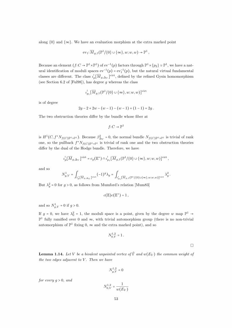
along 0 and ∞. We have an evaluation morphism at the extra marked point
ev1∶Mg,1(P1/0 ∪ ∞,w;w,w)→ P1 ,
Because an element (f ∶C → P1×P1) of ev−1(p) factors through P1×p2 ≃ P1, we have a nat-
ural identification of moduli spaces ev−1(p) = ev−11 (p), but the natural virtual fundamental
classes are different. The class ι!p[Mg,∆V]virt, defined by the refined Gysin homomorphism
(see Section 6.2 of [Ful98]), has degree g whereas the class
ι!p1[Mg,1(P1
/0 ∪ ∞,w;w,w)]virt
is of degree
2g − 2 + 2w − (w − 1) − (w − 1) + (1 − 1) = 2g .
The two obstruction theories differ by the bundle whose fiber at
f ∶C → P1
is H1(C, f∗Nf(C)∣P1×P1). Because β2∆V
= 0, the normal bundle Nf(C)∣P1×P1 is trivial of rank
one, so the pullback f∗Nf(C)∣P1×P1 is trivial of rank one and the two obstruction theories
differ by the dual of the Hodge bundle. Therefore, we have
ι!p[Mg,∆V]virt
= cg(E∗) ∩ ι!p1[Mg,1(P1
/0 ∪ ∞,w;w,w)]virt ,
and so
N1g,V = ∫
ι!p[Mg,∆V]virt
(−1)gλg = ∫ι!p1
[Mg,1(P1/0∪∞,w;w,w)]virtλ2g .
But λ2g = 0 for g > 0, as follows from Mumford’s relation [Mum83]
c(E)c(E∗) = 1 ,
and so N1g,V = 0 if g > 0.
If g = 0, we have λ20 = 1, the moduli space is a point, given by the degree w map P1 →
P1 fully ramified over 0 and ∞, with trivial automorphism group (there is no non-trivial
automorphism of P1 fixing 0, ∞ and the extra marked point), and so
N1,20,V = 1 .
Lemma 1.14. Let V be a bivalent unpointed vertex of Γ and w(EV ) the common weight of
the two edges adjacent to V . Then we have
N1,2g,V = 0
for every g > 0, and
N1,20,V =
1
w(EV )
53

for g = 0.
Proof. The argument is parallel to the one used to prove Lemma 1.13. The only difference
is that the vertex is no longer pointed and the invariant N1,2g,V is defined using the evaluation
map at one of the tangency point. The vanishing for g > 0 still follows from λ2g = 0. For
g = 0, the moduli space is a point, given by the degree w(EV ) map P1 → P1 fully ramified
over 0 and ∞, but now with an automorphism group Z/w(EV ) (the extra marked point
in Lemma 1.13 is no longer there to kill all non-trivial automorphisms). It follows that
N1,20,V = 1
w(EV ).
Corollary 1.15. Let h∶ Γ→ R2 be a parametrized tropical curve in T g∆,p.
• If there exists one bivalent vertex V of Γ with g(V ) ≠ 0, then
N∆,n
g,h= 0 .
• If g(V ) = 0 for all the bivalent vertices V of Γ, then
N∆,n
g,h=⎛⎜⎝
∏V ∈V (3)(Γ)
N1,2g(V ),V
⎞⎟⎠
⎛
⎝∏
E∈Ef (Γ)
w(E)⎞
⎠,
where the first product is over the trivalent vertices of Γ (or Γ), and the second product
is over the bounded edges of Γ (not Γ).
Proof. If Γ has a bivalent vertex V with g(V ) > 0, then, according to Lemmas 1.13 and 1.14,
we have N1,2g(V ),V
= 0 and so N∆,n
g,h= 0 by Proposition 1.12.
If g(V ) = 0 for all the bivalent vertices V of Γ, then, according to Lemma 1.13, we have
N1,2g(V ),V
= 1 for all the bivalent pointed vertices V of Γ and according to Lemma 1.14,
we have N1,2g(V ),V
= 1w(EV )
for all the bivalent unpointed vertices V of Γ . It follows that
Proposition 1.12 can be rewritten
N∆,n
g,h=⎛⎜⎝
∏V ∈V (3)(Γ)
N1,2g(V ),V
⎞⎟⎠
⎛⎜⎝
∏V ∈V (2up)(Γ)
1
w(EV )
⎞⎟⎠
⎛⎜⎝
∏E∈Ef (Γ)
w(E)⎞⎟⎠,
where the first product is over the trivalent vertices of Γ (which can be naturally identified
with the trivalent vertices of Γ) and the second product is over the bivalent unpointed
vertices of Γ. Recalling from Section 1.3.2 that the edges of Γ are obtained as subdivision
of the edges of Γ by adding the bivalent unpointed vertices, we have
⎛⎜⎝
∏V ∈V (2up)(Γ)
1
w(EV )
⎞⎟⎠
⎛⎜⎝
∏E∈Ef (Γ)
w(E)⎞⎟⎠= ∏E∈Ef (Γ)
w(E) .
54

1.6 Proof of the gluing formula
This Section is devoted to the proof of Proposition 1.12. Part of it is inspired the proof by
Chen [Che14a] of the degeneration formula for expanded stable log maps, and the proof by
Kim, Lho and Ruddat [KLR18] of the degeneration formula for stable log maps in degen-
erations along a smooth divisor. In Section 1.6.1, we define a cut morphism. Restricted to
some open substack of torically transverse stable maps, we show in Section 1.6.2 that the
cut morphism is etale, and in Section 1.6.3, that the cut morphism is compatible with the
natural obstruction theories of the pieces. Using in addition Proposition 1.10 and the results
of Section 1.2, we prove a gluing formula in Section 1.6.4. To finish the proof of Proposition
1.12, we explain in Section 1.6.5 how to organize the glued pieces.
1.6.1 Cutting
Let h∶ Γ → R2 be a parametrized tropical curve in T g∆,p. We denote V (2p)(Γ) the set of
bivalent pointed vertices of Γ and V (2up)(Γ) the set of bivalent unpointed vertices of Γ.
Evaluations evEV ∶Mg(V ),∆V→ DE at the tangency points dual to the bounded edges of Γ
give a morphism
ev(e)∶ ∏V ∈V (Γ)
Mg(V ),∆V→ ∏
E∈Ef (Γ)
(DE)2 ,
where DE is the divisor of X0 dual to an edge E of Γ.
Evaluations ev(p)V ∶Mg(V ),∆V
→ X∆Vat the extra marked points corresponding to the biva-
lent pointed vertices give a morphism
ev(p)∶ ∏V ∈V (Γ)
Mg(V ),∆V→ ∏
V ∈V (2p)(Γ)
X∆V.
Let
δ∶ ∏E∈Ef (Γ)
DE → ∏E∈Ef (Γ)
(DE)2
be the diagonal morphism. Let
ιP 0 ∶ (P 0= (P 0
V )V ∈V (2p)(Γ)) ∏
V ∈V (2p)(Γ)
X∆V,
be the inclusion morphism of P 0.
Using the fiber product diagram in the category of stacks
⨉V ∈V (Γ)
Mg(V ),∆V ∏V ∈V (Γ)
Mg(V ),∆V
⎛
⎝∏
E∈Ef (Γ)
DE
⎞
⎠× P 0
∏E∈Ef (Γ)
(DE)2 × ∏V ∈V (2p)(Γ)
X∆V,
(δ×ιP0)M
ev(e)×ev(p)
δ×ιP0
55

we define the substack ⨉V ∈V (Γ)Mg(V ),∆V
of ∏V ∈V (Γ)Mg(V ),∆V
consisting of curves whose
marked points keeping track of the tangency conditions match over the divisors DE and
whose extra marked points associated to the bivalent pointed vertices map to P 0.
Lemma 1.16. Let
C X0
ptM
ptN ,
f
π ν0
g
be a n-pointed genus g stable log map of type ∆ passing through P 0 and marked by h∶ Γ→ R2,
i.e. a point of Mh,P 0
g,n,∆. Let
Σ(C) Σ(X0)
Σ(ptM
) Σ(ptN) .
Σ(f)
Σ(π) Σ(ν0)
Σ(g)
be its tropicalization. For every b ∈ Σ(g)−1(1), let
Σ(f)b∶Σ(C)b → Σ(ν0)−1
(1) ≃ R2
be the fiber of Σ(f) over b. Let E be an edge of Γ and let Ef,b be the edge of Σ(C)b marked
by E. Then Σ(f)b(Ef,b) ⊂ h(E).
Proof. We recalled in Section 1.5 that the connected components of the complement of
the bivalent pointed vertices of Γ are trees with exactly one unbounded edge. We prove
mboxLemma 1.16 by induction, starting with the edges connected to the bivalent pointed
vertices and then we go through each tree following the orientation introduced in Section
1.5.
Let E be an edge of Γ adjacent to a bivalent pointed vertex V of Γ. Let P 0V ∈ X∆V
be
the corresponding marked point. As f is marked by h, we have an ordinary stable map
fV ∶CV → X∆V, a marked point xE in CV such that f(xE) ∈ DE and fV (CV ) contains
P 0V . We can assume that X∆V
= P1 × P1, DE = 0 × P1, β∆V= w(E)([P1] × [pt]), and
P 0V = (P 0
V,1, P0V,2) ∈ C∗×C∗ ⊂ P1×P1. Then fV factors through P1×P 0
V,2 and xE = (0, P 0V,2).
It follows that Σ(f)b(Ef,b) ⊂ h(E).
Let E be the outgoing edge of a trivalent vertex of Γ, of ingoing edges E1 and E2. By
the induction hypothesis, we know that Σ(f)b(E1f,b) ⊂ h(E1) and Σ(f)b(E
2f,b) ⊂ h(E2).
We conclude that Σ(f)b(Ef,b) ⊂ h(E) by an application of the balancing condition, as in
Proposition 30 (tropical Menelaus theorem) of Mikhalkin [Mik15].
For a stable log map
56

C X0
ptM
ptN
f
π ν0
g
marked by h, we have nodes of C in correspondence with the bounded edges of Γ. Cutting
C along these nodes, we obtain a morphism
cut∶Mh,P 0
g,n,∆ → ⨉V ∈V (Γ)
Mg(V ),∆V.
Let us give a precise definition of the cut morphism14. By definition of the marking, for every
vertex V of Γ, we have an ordinary stable map fV ∶CV → X∆V, such that the underlying
stable map to f is obtained by gluing together the maps fV along nodes corresponding to
the edges of Γ.
We have to give CV the structure of a log curve, and enhance fV to a log morphism. In
particular, we need to construct a monoid MV .
We fix a point b in the interior of Σ(g)−1(1). Let Σ(f)b∶Σ(C)b → R2 be the corresponding
parametrized tropical curve. Let Σ(C)V,b be the subgraph of Σ(C)b obtained by taking
the vertices of Σ(C)b dual to irreducible components of CV , the edges between them, and
considering the edges to other vertices of Σ(C)b as unbounded edges. Let Σ(f)V,b be the
restriction of Σ(f)b to Σ(C)V,b. It follows from Lemma 1.16 that one can view Σ(f)V,b as
a parametrized tropical curve of type ∆V to the fan of X∆V.
We defineMV as being the monoid whose dual is the monoid of integral points of the moduli
space of deformations of Σ(f)V,b preserving its combinatorial type15. Let iCV ∶CV → C
and iX∆V∶X∆V
→ X0 be the inclusion morphisms of ordinary (not log) schemes. The
parametrized tropical curves Σ(f)V encode a sheaf of monoidsMCV and a map f−1V MX∆V
→
MCV . We define a log structure on CV by
MCV =MCV ×i−1CVMC
i−1CVMC .
The natural diagram
f−1V MX∆V
MCV
f−1V i−1
X∆VMX0 i−1
CVMC
can be uniquely completed, by restriction, with a map
f−1V MX∆V
→MCV
14We are considering a stable log map over a point. It is a notational exercise to extend the argument toa stable log map over a general base, which is required to really define a morphism between moduli spaces
15The base monoid of a basic stable log map has always such description in terms of deformations oftropical curves. See Remark 1.18 and Remark 1.21 of [GS13] for more details
57

compatible with f−1V MX∆V
→MCV . This defines a log enhancement of fV and finishes the
construction of the cut morphism.
Remark: If one considers a general log smooth degeneration and if one applies the decom-
position formula, it is in general impossible to write the contribution of a tropical curves
in terms of log Gromov-Witten invariants attached to the vertices. This is already clear
at the tropical level. The theory of punctured invariants developed by Abramovich, Chen,
Gross, Siebert in [ACGS17b] is the correct extension of log Gromov-Witten theory which
is needed in order to be able to write down a general gluing formula. In our present case,
the Nishinou-Siebert toric degeneration is extremely special because it has been constructed
knowing a priori the relevant tropical curves. It follows from Lemma 1.16 that we always
cut edges contained in an edge of the polyhedral decomposition, and so we don’t have to
consider punctured invariants.
1.6.2 Counting log structures
We say that a map to X0 is torically transverse if its image does not contain any of the
torus fixed points of the toric components X∆V. In other words, its corestriction to each
toric surface X∆Vis torically transverse in the sense of Section 1.4.
Let Mh,P 0,
g,n,∆ be the open locus of Mh,P 0
g,n,∆ formed by the torically transverse stable log maps
to X0, and for every vertex V of Γ, let M
g(V ),∆Vbe the open locus of Mg(V ),∆V
formed by
the torically transverse stable log maps to X∆V. The morphism cut restricts to a morphism
cut∶Mh,P 0,
g,n,∆ → ⨉V ∈V (Γ)
M
g(V ),∆V.
Proposition 1.17. The morphism
cut∶Mh,P 0,
g,n,∆ → ⨉V ∈V (Γ)
M
g(V ),∆V
is etale of degree
∏E∈Ef (Γ)
w(E) ,
where the product is over the bounded edges of Γ.
Proof. Let (fV ∶CV → X∆V)V ∈ ⨉V ∈V (Γ)
M
g(V ),∆V. We have to glue the stable log maps
fV together. Because we are assuming that the maps fV are torically transverse, the image
in X0 by fV of the curves CV is away from the torus fixed points of the components X∆V.
The gluing operation corresponding to the bounded edge E of Γ happens entirely along the
torus C∗ contained in the divisor DE .
It follows that it is enough to study the following local model. Denote ` ∶= `(E)w(E),
where `(E) is the length of E and w(E) the weight of E. Let XE be the toric variety
Spec C[x, y, u±, t]/(xy = t`), equipped with a morphism νE ∶XE → C given by the coordinate
t. Using the natural toric divisorial log structures on XE and C, we define by restriction a
58

log structure on the special fiber X0,E ∶= ν−1E (0) and a log smooth morphism to the standard
log point ν0,E ∶X0,E → ptN. The scheme underlying X0,E has two irreducible components,
X1,E ∶= Cx ×C∗u and X2,E ∶= Cy ×C∗
u, glued along the smooth divisor DE ∶= C∗
u. We endow
X1,E and X2,E with their toric divisorial log structures.
Let f1∶C1/ptM1
→ X1,E be the restriction to X1,E of a torically transverse stable log map
to some toric compactification of X1,E , with one point p1 of tangency order w(E) along DE ,
and let f2∶C2/ptM2
→ X2,E be the restriction to X2,E of a torically transverse stable log
map to some toric compactification of X2,E , with one point p2 of tangency order w(E) along
DE . We assume that f(p1) = f(p2) and so we can glue the underlying maps f1∶C1 →X1,E
and f2∶C2 →X2,E to obtain a map f ∶C →X0,E where C is the curve obtained from C1 and
C2 by identification of p1 and p2. We denote p the corresponding node of C. We have to
show that there are w(E) ways to lift this map to a log map in a way compatible with the
log maps f1 and f2 and with the basic condition. If C1 and C2 had no component contracted
to f(p) ∈ DE , this would follow from Proposition 7.1 of Nishinou, Siebert [NS06]. But we
allow contracted components, so we have to present a variant of the proof of Proposition 7.1
of [NS06].
We first give a tropical description of the relevant objects. The tropicalization of X0,E is
the cone Σ(X0,E) = Hom(MX0,E ,f(p),R⩾0). It is the fan of XE , a two-dimensional cone
generated by rays ρ1 and ρ2 dual to the divisors X1,E and X2,E . The toric description
XE = Spec C[x, y, u±, t]/(xy = t`) defines a natural chart for the log structure of X0,E .
Denote sx, sy, st the corresponding elements ofMX0,E ,f(p) and sx, sy, st their projections in
MX0,E ,f(p). We have sxsy = s`t. Seeing elements ofMX0,E ,f(p) as functions on Σ(X0,E), we
have ρ1 = s−1y (0), ρ2 = s
−1x (0) and st∶Σ(X0,E) → R⩾0 is the tropicalization of the projection
X0,E → ptN. Level sets s−1t (c) are line segments [P1, P2] in Σ(X0,E), connecting a point P1
of ρ1 to a point P2 of ρ2, of length `c.
Denote C1,E and C2,E the irreducible components of C1 and C2 containing p1 and p2
respectively. We can see them as the two irreducible components of C meeting at the node
p. Fix j = 1 or j = 2. The tropicalization of Cj/ptMj
is a family Σ(Cj) of tropical curves
Σ(Cj)b parametrized by b ∈ Σ(ptMj
) = Hom(Mj ,R⩾0). Let Vj,E be the vertex of these
tropical curves dual to the irreducible component Cj,E . The image Σ(fj)(Vj,E) of Vj,E
by the tropicalization Σ(fj) of fj is a point in the tropicalization Σ(Xj,E) = R⩾0. This
induces a map Hom(Mj ,R⩾0) → R⩾0 defined by an element vj ∈Mj . The component Cj,Eis contracted by fj onto fj(pj) if and only if vj ≠ 0. In other words, vj is the measure
according to the log structures of “how” Cj,E is contracted by fj . The marked point pj on
Cj,E defines an unbounded edge Ej , of weight w(E), whose image by Σ(fj) is the unbounded
interval [Σ(fj)(Vj,E),+∞) ⊂ Σ(Xj,E) = R⩾0.
We explain now the gluing at the tropical level. Let j = 1 or j = 2. Let [0, `j] ⊂ Σ(Xj,E) = R⩾0
be an interval. If c is a large enough positive real number, we denote ϕjc∶ [0, `j] s−1t (c) =
[P1, P2] the linear inclusion such that ϕjc(0) = Pj and ϕjc([0, `j]) is a subinterval of [P1, P2]
of length `j . Let bj ∈ Σ(ptMj
). There exists `j large enough such that all images by Σ(fj)
of vertices of Σ(fj)bj are contained in [0, `j] ⊂ Σ(Xj,E) = R⩾0.
59

For c large enough, the line segments ϕ1c([0, `1]) and ϕ2
c([0, `2]) are disjoint. We have
[P1, P2]
= [P1, ϕ1c(Σ(f1)(V1))) ∪ [ϕ1
c(Σ(f1)(V1)), ϕ2c(Σ(f2)(V2))] ∪ (ϕ2
c(Σ(f2)(V2)), P2] .
We construct a new tropical curve Σb1,b2,c by removing the unbounded edges E1 and
E2 of Σ(f1)b1 and Σ(f2)b2 , and gluing the remaining curves by an edge F connecting
V1,E and V2,E , of weight w(E), and length 1w(E)
times the length of the line segment
[ϕ1c(Σ(f1)(V1)), ϕ
2c(Σ(f2)(V2))]. We construct a tropical map Σb1,b2,c → Σ(X0,E) using
Σ(f1)b1 , Σ(f2)b2 and mapping the edge F to [ϕ1c(Σ(f1)(V1)), ϕ
2c(Σ(f2)(V2))]. We define
M as being the monoid whose dual is the monoid of integral points of the moduli space of
deformations of these tropical maps.
We have M = M1 ⊕M2 ⊕ N. The element (0,0,1) ∈ M defines the function on the
moduli space of tropical curves Σ(ptM
) = Hom(M,R⩾0) given by the length of the glu-
ing edge F . The function given by 1`
times the length of the line segment [P1, P2] de-
fines an element sMt ∈ M. The morphism of monoids N → M, 1 ↦ sMt , induces a map
g∶ptM→ ptN. The decomposition of [P1, P2] into the three intervals [P1, ϕ
1c(Σ(f1)(V1))),
[ϕ1c(Σ(f1)(V1)), ϕ
2c(Σ(f2)(V2))] and (ϕ2
c(Σ(f2)(V2)), P2], implies the relation
` sMt = (v1,0,0) + (0,0,w(E)) + (0, v2,0)
in M =M1 ⊕M2 ⊕N.
r
r
@@
@@@
@@
@@
rr
ρ1
ρ2
P2
P1
ϕ1c(Σ(f1)(V1))
ϕ2c(Σ(f2)(V2))
Σ(X0,E)
From the tropical description of the gluing and from the fact that we want to obtain a basic
log map, we find that there is a unique structure of log smooth curve C/ptM
compatible with
the structures of log smooth curves on C1 and C2. As p is a node of C, we have for the ghost
sheaf of C at p: MC,p =M ⊕N N2, with N → N2, 1 ↦ (1,1), and N →M =M1 ⊕M2 ⊕N,
1↦ ρp = (0,0,1).
It remains to lift f ∶C →X0,E to a log map f ∶C →X0,E such that the diagram
C X0,E
ptM
ptN
f
π ν0,E
g
60

commutes. The restriction of f to Cj/ptMj
has to coincide with fj , for j = 1 and j = 2. It
follows from the explicit description of M and MC that such f exists and is unique away
from the node p.
It follows from the tropical description of the gluing that at the ghost sheaves level, f at p
is given by
f∶MX0,E ,f(p) →MC,p =M⊕N N2
= (M1 ⊕M2 ⊕N)⊕N N2
sx ↦ ((v1,0,0), (w(E),0))
sy ↦ ((0, v2,0), (0,w(E)))
st ↦ π(sMt ) = (sMt , (0,0)) .
The relation ` sMt = (v1, v2,w(E)) in M =M1 ⊕M2 ⊕N implies that
f(sx) + f
(sy) = ((v1, v2,0), (w(E),w(E))) = ((v1, v2,w(E)), (0,0))
= f(`sMt ) ,
and so that this map is indeed well-defined.
The log maps f1∶C1/ptM1→X1,E and f2∶C2/pt
M2→X2,E define morphisms
f 1∶MX1,E ,f(p1) →MC1,p1 ,
and
f 2∶MX2,E ,f(p2) →MC2,p2 .
For j = 1 or j = 2, let Mj ⊕ N → OCj ,pj be a chart of the log structure of Cj at pj . This
realizesMCj ,pj as a quotient of (Mj ⊕N)⊕O∗C,p. Denote sj,m ∈MCj ,pj the image of (m,1)
for m ∈Mj ⊕N.
We fix a coordinate u on C1 near p1 such that
f 1(sx) = s1,(v1,0)uw(E)
and a coordinate v on C2 near p2 such that
f 2(sy) = s2,(v2,0)vw(E) .
We are trying to define some f ∶MX0,E ,f(p) →MC,p, lift of f, compatible with f 1 and f 2.
For every ζ a w(E)-th root of unity, the map
M⊕N N2→ OC,p
(m, (a, b))↦
⎧⎪⎪⎨⎪⎪⎩
ζauavb if m = 0
0 if m ≠ 0
defines a chart for the log structure of C at p. This realizes MC,p as a quotient of (M⊕N
61

N2) ⊕ O∗C,p. Denote sζm ∈ MC,p the image of (m,1) for m ∈ M ⊕N N2. Remark that
sζ((v1,0,0),(0,0))
, sζ((0,v2,0),(0,0))
and sζ((0,0,0),(1,1))
are independent of ζ and we denote them
simply as s((v1,0,0),(0,0)), s((0,v2,0),(0,0)) and s((0,0,0),(1,1)).
Then
f ,ζ ∶MX0,E ,f(p) →MC,p
sx ↦ sζ((v1,0,0),(w(E),0))
sy ↦ sζ((0,v2,0),(0,w(E)))
st ↦ π((sMt ,1))
is a lift of f, compatible with f 1 and f 2.
Assume that f ,ζ ≃ f ,ζ′
for ζ and ζ ′ two w(E)-th roots of unity. It follows from the com-
patibility with f 1 and f 2 that there exists ϕ1 ∈ O∗C,p and ϕ2 ∈ O
∗C,p such that sζ
′
((0,0,0),(1,0))=
ϕ1sζ((0,0,0),(0,1))
and sζ′
((0,0,0),(0,1))= ϕ2s
ζ((0,0,0),(0,1))
. It follows from the definition of the
charts that ϕ1 = ζ ′ζ−1 in OC1,p1 and ϕ2 = 1 in OC2,p2 . Compatibility with ptM→ ptN
implies that ϕ1ϕ2 = 1. This implies that ϕ1 = ϕ2 = 1 and ζ = ζ ′.
It remains to show that any f , lift of f
compatible with f 1 and f 2, is of the form f ,ζ for
some ζ a w(E)-th root of unity. For such f , there exists unique s′(1,0) ∈MC,p and s′
(0,1) ∈
MC,p such that αC(s′(1,0)) = u, αC(s′
(0,1)) = v, and f (sx) = s((v1,0,0),(0,0))(s′(1,0))
w(E) and
f (sy) = s((0,v2,0),(0,0))(s′(0,1))
w(E). From sxsy = s`t, we get (s′
(1,0)s′(0,1))
w(E) = sw(E)
((0,0,0),(1,1))
and so s′(1,0)s
′(0,1) = ζ
−1s((0,0,0),(1,1)) for some ζ a w(E)-th root of unity. It is now easy to
check that s′(1,0) = ζ
−1sζ((0,0,0),(1,0))
, s′(0,1) = s
ζ((0,0,0),(0,1))
and f = f ,ζ .
Remarks:
• When v1 = v2 = 0, i.e. when the components C1,E and C2,E are not contracted, the
above proof reduces to the proof of Proposition 7.1 of [NS06] (see also the proof of
Proposition 4.23 of [Gro11]). In general, log geometry remembers enough information
about the contracted components, such as v1 and v2, to make possible a parallel
argument.
• The gluing of stable log maps along a smooth divisor is discussed in Section 6 of
[KLR18], proving the degeneration formula along a smooth divisor. In the above
proof, we only have to glue along one edge connecting two vertices. In Section 6 of
[KLR18], further work is required to deal with pair of vertices connected by several
edges.
62

1.6.3 Comparing obstruction theories
As in the previous Section 1.6.2, let Mh,P 0,
g,n,∆ be the open locus of Mh,P 0
g,n,∆ formed by the
torically transverse stable log maps to X0, and for every vertex V of Γ, let M
g(V ),∆Vbe the
open locus of Mg(V ),∆Vformed by the torically transverse stable log maps to X∆V
. The
morphism cut restricts to a morphism
cut∶Mh,P 0,
g,n,∆ → ⨉V ∈V (Γ)
M
g(V ),∆V.
The goal of the present Section is to use the morphism cut to compare the virtual classes
[Mh,P 0,
g,n,∆ ]virt and [M
g(V ),∆V]virt, which are obtained by restricting the virtual classes [M
h,P 0
g,n,∆]virt
and [Mg(V ),∆V]virt to the open loci of torically transverse stable log maps.
Recall that X0 = ν−1(0), where ν∶XP∆,n→ A1. Following Section 4.1 of [ACGS17a], we
define X0 ∶= AX ×AA1 0, where AX and AA1 are Artin fans, see Section 2.2 of [ACGS17a].
It is an algebraic log stack over ptN. There is a natural morphism X0 → X0.
Following Section 4.5 of [ACGS17a], let Mhg,n,∆ be the stack of n-pointed genus g prestable
basic log maps to X0/ptN marked by h and of type ∆. There is a natural morphism of stacks
Mh,P 0
g,n,∆ →Mhg,n,∆ . Let π∶C → M
h,P 0
g,n,∆ be the universal curve and let f ∶C → X0/ptN be the
universal stable log map. According to Proposition 4.7.1 and Section 6.3.2 of [ACGS17a],
the virtual fundamental class [Mh,P 0
g,n,∆]virt is defined by E, the cone of the morphism
(ev(p))∗LιP0 [−1]→ (Rπ∗f∗TX0∣X0
)∨, seen as a perfect obstruction theory relative to Mhg,n,∆.
Here, TX0∣X0is the relative log tangent bundle, and LιP0 = ⊕V ∈V (2p)(Γ)
(TX∆V∣P 0V)∨[1] is the
cotangent complex of ιP 0 . As X0 is log etale over ptN, we have TX0∣X0= TX0∣ptN
. We denote
E the restriction of E to the open locus Mh,P 0,
g,n,∆ of torically transverse stable log maps.
For every vertex V of Γ, let πV ∶CV →Mg(V ),∆Vbe the universal curve and let fV ∶CV →X∆V
be the universal stable log map. Let AX∆Vbe the Artin fan of X∆V
and let Mg(V ),∆Vbe
the stack of prestable basic log maps to AX∆V, of genus g(V ) and of type ∆V . There is a
natural morphism of stacks Mg(V ),∆V→Mg(V ),∆V
. According to Section 6.1 of [AW13], the
virtual fundamental class [Mg(V ),∆V]virt is defined by (R(πV )∗f
∗V TX∆V
)∨, seen as a perfect
obstruction theory relative to Mg(V ),∆V. Here, TX∆V
is the log tangent bundle.
Recall that ⨉V ∈V (Γ)
Mg(V ),∆Vis defined by the fiber product diagram
⨉V ∈V (Γ)
Mg(V ),∆V ∏V ∈V (Γ)
Mg(V ),∆V
⎛
⎝∏
E∈Ef (Γ)
DE
⎞
⎠× P 0
∏E∈Ef (Γ)
(DE)2 × ∏V ∈V (2p)(Γ)
X∆V.
(δ×ιP0)M
ev(e)×ev(p)
ev(e)×ev(p)
δ×ιP0
We compare the deformation theory of the individual stable log maps fV and the deformation
theory of the stable log maps fV constrained to match at the gluing nodes. Let F be the
63

cone of the natural morphism
(ev(e)× ev(p)
)∗Lδ×ιP0 [−1]→ (δ × ιP 0)
∗M ( ⊠
V ∈V (Γ)
(R(πV )∗f∗V TX∆V
)∨) ,
where Lδ×ιP0 is the cotangent complex of the morphism δ× ιP 0 . It defines a perfect obstruc-
tion theory on ⨉V ∈V (Γ)
Mg(V ),∆Vrelative to ∏
V ∈V (Γ)
Mg(V ),∆V, whose corresponding virtual
fundamental class is, using Proposition 5.10 of [BF97],
(δ × ιP 0)!∏
V ∈V (Γ)
[Mg(V ),∆V]virt ,
where (δ × ιP 0)! is the refined Gysin homomorphism (see Section 6.2 of [Ful98]). We denote
F the restriction of F to the open locus ⨉V ∈V (Γ)M
g(V ),∆Vof torically transverse stable log
maps.
The cut operation naturally extends to prestable log maps to X0/ptN marked by h, and so
we have a commutative diagram
Mh,P 0,
g,n,∆ ⨉V ∈V (Γ)
M
g(V ),∆V
Mhg,n,∆ ∏
V ∈V (Γ)
Mg(V ),∆V.
cut
µ
cutC
By Proposition 1.17, the morphism cut is etale and so (cut)∗F defines a perfect obstruc-
tion theory on Mh,P 0,
g,n,∆ relative to ∏V ∈V (Γ)
Mg(V ),∆V.
The maps Mh,P 0,
g,n,∆
µÐ→ Mh
g,n,∆(X0/ptN)cutCÐÐ→ ∏
V ∈V (Γ)
Mg(V ),∆Vdefine an exact triangle of
cotangent complexes
LMh,P0,
g,n,∆ ∣ ∏V ∈V (Γ)
Mg(V ),∆V
→ LMh,P0,
g,n,∆ ∣Mhg,n,∆
→ µ∗LMhg,n,∆
∣ ∏V ∈V (Γ)
Mg(V ),∆V
[1][1]Ð→ .
Adding the perfect obstruction theories (cut)∗F and E, we get a diagram
(cut)∗F E
LMh,P0,
g,n,∆ ∣ ∏V ∈V (Γ)
Mg(V ),∆V
LMh,P0,
g,n,∆ ∣Mhg,n,∆
µ∗LMhg,n,∆
∣ ∏V ∈V (Γ)
Mg(V ),∆V
[1] .[1]
Proposition 1.18. The above diagram can be completed into a morphism of exact triangles
64

(cut)∗F E µ∗LMhg,n,∆
∣ ∏V ∈V (Γ)
Mg(V ),∆V
[1] .
LMh,P0,
g,n,∆ ∣ ∏V ∈V (Γ)
Mg(V ),∆V
LMh,P0,
g,n,∆ ∣Mhg,n,∆
µ∗LMhg,n,∆
∣ ∏V ∈V (Γ)
Mg(V ),∆V
[1] .
[1]
[1]
Proof. Denote X0 , X
∆V, D
E the objects obtained from X0, X∆V, DE by removing the
torus fixed points of the toric surfaces X∆V. Denote ιX
∆Vthe inclusion morphism of X
∆V
in X0 .
If E is a bounded edge of Γ, we denote V 1E and V 2
E the two vertices of E. Let F be the sheaf
on the universal curve C∣Mh,P0,
g,n,∆
defined as the kernel of
⊕V ∈V (Γ)
f∗(ιX
∆V)∗TX
∆V→ ⊕
E∈Ef (Γ)
(ιE)∗(evE)∗TD
E
(sV )V ↦ (sV 1E∣D
E− sV 2
E∣D
E)E ,
where evE is the evaluation at the node pE dual to E, and ιE the section of C given
by pE . It follows from the exact triangle obtained by applying Rπ∗ to the short exact
sequence defining F and from Lδ = ⊕E∈Ef (Γ)T ∨DE [1] that (cut)∗F is given by the cone of
the morphism (ev(p))∗LιP0 [−1] → (Rπ∗F)∨. So in order to compare E and (cut)∗F, we
have to compare f∗TX
0 ∣ptNand F . The sheaf f∗TX
0 ∣ptNcan be written as the kernel of
f∗ ⊕V ∈V (Γ)
(ιX
∆V)∗(ιX
∆V)∗TX
0 ∣ptN→ ⊕
E∈Ef (Γ)
(ιE)∗(evE)∗TX
0 ∣ptN.
(sV )V ↦ (sV 1E∣D
E− sV 2
E∣D
E)E .
Remark that because X0 is the special fiber of a toric degeneration, all the log tangent
bundles TX0, TX∆V
, TDE are free sheaves (see e.g. Section 7 of [NS06]). In particular, the
restrictions (ιX
∆V)∗TX
0 ∣ptN→ TX
∆Vare isomorphisms, the restriction
⊕E∈Ef (Γ)
(evE)∗TX
0 ∣ptN→ ⊕
E∈Ef (Γ)
(evE)∗TD
E
has kernel ⊕E∈Ef (Γ)(evE)∗OD
Eand so there is an induced exact sequence
0→ f∗TX
0 ∣ptN→ F → ⊕
E∈Ef (Γ)
(ιE)∗(evE)∗OD
E→ 0 ,
which induces an exact triangle on Mh,P 0
g,n,∆ :
(cut)∗F→ E
→ ⊕E∈Ef (Γ)
(evE)∗OD
E[1]
[1]Ð→ .
It remains to check the compatibility of this exact triangle with the exact triangle of cotan-
65

gent complexes. We have
µ∗LMhg,n,∆
∣ ∏V ∈V (Γ)
Mg(V ),∆V
= ⊕E∈Ef (Γ)
(ιE)∗OpE .
Indeed, restricted to the locus of torically transverse stable log maps, cutC is smooth, and,
given a torically transverse stable log map to X0/ptN, a basis of first order infinitesimal
deformations fixing its image by cutC in ∏V ∈V (Γ)Mg(V ),∆V
is indexed by the cutting nodes.
The dual of the natural map
⊕E∈Ef (Γ)
(evE)∗OD
E→ µ∗L
Mhg,n,∆
∣ ∏V ∈V (Γ)
Mg(V ),∆V
= ⊕E∈Ef (Γ)
(ιE)∗OpE
sends the canonical first order infinitesimal deformation indexed by the cutting node pE
to the canonical summand OD
Ein the normal bundle to the diagonal ∏E∈Ef (Γ)
DE in
∏E∈Ef (Γ)(D
E)2, and so is an isomorphism. This guarantees the compatibility with the
exact triangle of cotangent complexes.
Remark: Restricted to the open locus of torically transverse stable maps, the discussion is
essentially reduced to a collection of gluings along the smooth divisors DE . A comparison of
the obstruction theories in the context of the degeneration formula along a smooth divisor
is given with full details in Section 7 of [KLR18].
Proposition 1.19. We have
(cut)∗ ([Mh,P 0,
g,n,∆ ]virt
)
=⎛⎜⎝
∏E∈Ef (Γ)
w(E)⎞⎟⎠
⎛⎜⎝(δ × ιP 0)
!M ∏V ∈V (Γ)
[M
g(V ),∆V]virt
⎞⎟⎠.
Proof. It follows from Proposition 1.18 and from Theorem 4.8 of [Man12] that the relative
obstruction theories E and (cut)∗F define the same virtual fundamental class on Mh,P 0,
g,n,∆ .
By Proposition 1.17, cut is etale, and so, by Proposition 7.2 of [BF97], the virtual funda-
mental class defined by (cut)∗F is the image by (cut)∗ of the virtual fundamental class
defined by F. It follows that
[Mh,P 0,
g,n,∆ ]virt
= (cut)∗(δ × ιP 0)!M ∏V ∈V (Γ)
[M
g(V ),∆V]virt .
According to Proposition 1.17, the morphism cut is etale of degree ∏E∈Ef (Γ)w(E), and so
the result follows from the projection formula.
1.6.4 Gluing
Recall that we have the morphism
(δ × ιP 0)M ∶ ⨉V ∈V (Γ)
Mg(V ),∆V→ ∏
V ∈V (Γ)
Mg(V ),∆V.
66

For every V ∈ V (Γ), we have a projection morphism
prV ∶ ∏V ′∈V (Γ)
Mg(V ′),∆V ′→Mg(V ),∆V
.
On each moduli space Mg(V ),∆V, we have the top lambda class (−1)g(V )λg(V ).
Proposition 1.20. We have
N∆,n
g,h= ∫
(δ×ιP0)! ∏V ∈V (Γ)
[Mg(V ),∆V]virt
(δ × ιP 0)∗M ∏V ∈V (Γ)
pr∗V ((−1)g(V )λg(V )) .
Proof. By definition (see Section 1.3.3), we have
N∆,n
g,h= ∫
[Mh,P0
g,n,∆]virt(−1)g−g∆,nλg−g∆,n
.
Using the gluing properties of lambda classes given by Lemma 1.6, we obtain that
(−1)g−g∆,nλg−g∆,n= (cut)∗(δ × ιP 0)
∗M ∏V ∈V (Γ)
pr∗V ((−1)g(V )λg(V )) .
It follows from the projection formula that
N∆,n
g,h= ∫
(cut)∗[Mh,P0
g,n,∆]virt(δ × ιP 0)
∗M ∏V ∈V (Γ)
pr∗V ((−1)g(V )λg(V )) .
According to Proposition 1.19, the cycles
(cut)∗ ([Mh,P 0
g,n,∆]virt
)
and⎛⎜⎝
∏E∈Ef (Γ)
w(E)⎞⎟⎠
⎛⎜⎝(δ × ιP 0)
!∏
V ∈V (Γ)
[Mg(V ),∆V]virt
⎞⎟⎠
have the same restriction to the open substack
⨉V ∈V (Γ)
M
g(V ),∆V
of
⨉V ∈V (Γ)
Mg(V ),∆V.
It follows, by Proposition 1.8 of [Ful98], that their difference is rationally equivalent to a
cycle supported on the closed substack
Z ∶=⎛
⎝⨉
V ∈V (Γ)
Mg(V ),∆V
⎞
⎠−⎛
⎝⨉
V ∈V (Γ)
M
g(V ),∆V
⎞
⎠.
67

If we have
(fV ∶CV →X∆V)V ∈V (Γ)
∈ Z ,
then at least one stable log map fV ∶CV →X∆Vis not torically transverse. By Lemma 1.16,
the unbounded edges of the tropicalization of fV are contained in the rays of the fan of X∆V.
It follows that we can apply Proposition 1.10 to obtain that at least one of the source curves
CV contains a non-trivial cycle of components. By the vanishing result of Lemma 1.7, this
implies that
∫Z(δ × ιP 0)
∗M ∏V ∈V (Γ)
pr∗V ((−1)g(V )λg(V )) = 0 .
It follows that
∫(cut)∗[M
h,P0
g,n,∆]virt(δ × ιP 0)
∗M ∏V ∈V (Γ)
pr∗V ((−1)g(V )λg(V ))
= ∫(δ×ιP0)! ∏
V ∈V (Γ)
[Mg(V ),∆V]virt
(δ × ιP 0)∗M ∏V ∈V (Γ)
pr∗V ((−1)g(V )λg(V )) .
This finishes the proof of Proposition 1.20.
1.6.5 Identifying the pieces
Proposition 1.21. We have
∫(δ×ιP0)! ∏
V ∈V (Γ)
[Mg(V ),∆V]virt
(δ × ιP 0)∗M ∏V ∈V (Γ)
pr∗V ((−1)g(V )λg(V )) = ∏V ∈V (Γ)
N1,2g(V ),V
.
Proof. Using the definitions of δ and ιP 0 , we have
∫(δ×ιP0)! ∏
V ∈V (Γ)
[Mg(V ),∆V]virt
(δ × ιP 0)∗M ∏V ∈V (Γ)
pr∗V ((−1)g(V )λg(V ))
= ∫∏
V ∈V (Γ)
[Mg(V ),∆V]virt
(ev(p))∗([P 0
])(ev(e))∗([δ]) ∏
V ∈V (Γ)
pr∗V ((−1)g(V )λg(V )) ,
where
[P 0] = ∏
V ∈V (2p)(Γ)
P 0V ∈ A∗
⎛⎜⎝
∏V ∈V (2p)(Γ)
X∆V
⎞⎟⎠
is the class of P 0 and
[δ] ∈ A∗⎛⎜⎝
∏E∈Ef (Γ)
(DE)2⎞⎟⎠
is the class of the diagonal ∏E∈Ef (Γ)DE . As each DE is a projective line, we have
[δ] = ∏E∈Ef (Γ)
(ptE × 1 + 1 × ptE) ,
68

where ptE ∈ A1(DE) is the class of a point.
We fix an orientation of edges of Γ as described in Section 1.5. In particular, every trivalent
vertex has two ingoing and one outgoing adjacent edges, every bivalent pointed vertex has
two outgoing adjacent edges, every bivalent unpointed vertex has one ingoing and one outgo-
ing edges. For every bounded edge E of Γ, we denote V sE the source vertex of E and V tE the
target vertex of E, as defined by the orientation. Furthermore, the connected components of
the complement of the bivalent pointed vertices of Γ are trees with exactly one unbounded
edge.
We argue that the effect of the insertion (ev(p))∗([P 0])(ev(e))∗([δ]) can be computed in
terms of the combinatorics of ingoing and outgoing edges of Γ16. More precisely, we claim
that the only term in
(ev(e))∗([δ]) = ∏
E∈Ef (Γ)
((evEV sE)∗(ptE) + (evEV t
E)∗(ptE)) ,
giving a non-zero contribution after multiplication by
⎛⎜⎝
∏V ∈V (2p)(Γ)
(ev(p)V )
∗(P 0
V )⎞⎟⎠
∏V ∈V (Γ)
pr∗V ((−1)g(V )λg(V ))
and integration over ∏V ∈V (Γ)[Mg(V ),∆V
]virt is ∏E∈Ef (Γ)(evEV t
E)∗(ptE).
We prove this claim by induction, starting at the bivalent pointed vertices, where things are
constrained by the marked points P 0, and propagating these constraints following the flow
on Γ defined by the orientation of edges.
Let V be a bivalent pointed vertex, E an edge adjacent to V and V ′ the other ver-
tex of E. The edge E is outgoing for V and ingoing for V ′, so V ′ = V tE . We have in
(ev(p))∗([P 0])(ev(e))∗([δ]) a corresponding factor
(ev(p)V )
∗(P 0
V ) ((evEV )∗(ptE) + (evEV ′)
∗(ptE)) .
But
(ev(p)V )
∗(P 0
V )(evEV )∗(ptE)(−1)g(V )λg(V ) = 0
for dimension reasons (its insertion over Mg(V ),∆Vdefines an enumerative problem of virtual
dimension −1) and so only the factor
(ev(p)V )
∗(P 0
V )(evEV ′)∗(ptE)
survives, which proves the initial step of the induction.
Let E be an outgoing edge of a trivalent vertex V , of ingoing edges E1 and E2. Let V tEbe the target vertex of E. By the induction hypothesis, every possibly non-vanishing term
16It is essentially a cohomological reformulation and generalization of the way the gluing is organized inMikhalkin’s proof of the tropical correspondence theorem, [Mik05].
69

contains the insertion of (evE1
V )∗(ptE1)(evE2
V )∗(ptE2). But
(evE1
V )∗(ptE1)(evE
2
V )∗(ptE2)(evEV )
∗(ptE)(−1)g(V )λg(V ) = 0
for dimension reasons (its insertion over Mg(V ),∆Vdefines an enumerative problem of virtual
dimension −1) and so only the factor
(evE1
V )∗(pt1
E)(evE2
V )∗(pt2
E)(evEV tE)∗(ptE)
survives.
Let E be an outgoing edge of a bivalent unpointed vertex V , of ingoing edges E1. Let V tE the
target vertex of E. By the induction hypothesis, every possibly non-vanishing term contains
the insertion of (evE1
V )∗(ptE1). But
(evE1
V )∗(ptE1)(evEV )
∗(ptE)(−1)g(V )λg(V ) = 0
for dimension reasons (its insertion over Mg(V ),∆Vdefines an enumerative problem of virtual
dimension −1) and so only the factor
(evE1
V )∗(ptE1)(evEV t
E)∗(ptE)
survives. This finishes the proof by induction of the claim.
Using the notations introduced in Section 1.5, we can rewrite
∏E∈Ef (Γ)
(evEV tE)∗(ptE)
as
⎛⎜⎝
∏V ∈V (3)(Γ)
(evEin,1V
V )∗(ptEin,1
V)(ev
Ein,2V
V )∗(ptEin,2
V)⎞⎟⎠
⎛⎜⎝
∏V ∈V (2up)(Γ)
(evEinV
V )∗(ptEin
V)⎞⎟⎠,
and so we proved
∫(δ×ιP0)! ∏
V ∈V (Γ)
[Mg(V ),∆V]virt
(δ × ιP 0)∗M ∏V ∈V (Γ)
pr∗V ((−1)g(V )λg(V ))
=⎛⎜⎝
∏V ∈V (3)(Γ)
N1,2g(V ),V
⎞⎟⎠
⎛⎜⎝
∏V ∈V (2p)(Γ)
N1,2g(V ),V
⎞⎟⎠
⎛⎜⎝
∏V ∈V (2up)(Γ)
N1,2g(V ),V
⎞⎟⎠.
This finishes the proof of Proposition 1.21.
1.6.6 End of the proof of the gluing formula
The gluing identity given by Proposition 1.12 follows from the combination of Proposition
1.20 and Proposition 1.21.
70

1.7 Vertex contribution
In this Section, we evaluate the invariants N1,2g,V attached to the vertices V of Γ and appearing
in the gluing formula of Corollary 1.15. The first step, carried out in Section 1.7.1 is to
rewrite these invariants in terms of more symmetric invariants Ng,V depending only on the
multiplicity of the vertex V . In Section 1.7.2, we use the consistency of the gluing formula
to deduce non-trivial relations between these invariants and to reduce the question to the
computation of the invariants attached to vertices of multiplicity one and two. Invariants
attached to vertices of multiplicity one and two are explicitly computed in Section 1.7.3
and this finishes the proof of Theorem 1. Modifications needed to prove Theorem 1.5 are
discussed at the end of Section 1.7.4.
1.7.1 Reduction to a function of the multiplicity
The gluing formula of the previous Section, Corollary 1.15, expresses the log Gromov-Witten
invariant N∆,ng,h attached to a parametrized tropical curve h∶Γ → R2 as a product of log
Gromov-Witten N1,2g(V ),V
attached to the trivalent vertices V of Γ, and of the weights w(E)
of the edges E of Γ. The definition of N1,2g(V ),V
given in Section 1.5 depends on a specific
choice of orientation on the edges of Γ. In particular, the definition of N1,2g(V ),V
does not
treat the three edges adjacent to V in a symmetric way.
Let Ein,1V and Ein,2
V be the two ingoing edges adjacent to V , and let EoutV be the outgoing
edge adjacent to V . Let DEin,1V
, DEin,2V
and DEoutV
be the corresponding toric divisors of
X∆V. We have evaluation morphisms
ev = (ev1, ev2, evout)∶Mg,∆V→DEin,1
V×DEin,2
V×DEout
V.
In Section 1.5, we defined
N1,2g,V = ∫
[Mg,∆V]virt
(−1)gλgev∗1(pt1)ev∗2(pt2) ,
where pt1 ∈ A1(DEin,1V
) and pt2 ∈ A1(DEin,2V
) are classes of a point on DEin,1V
and DEin,2V
respectively.
But one could similarly define
N2,outg,V ∶= ∫
[Mg,∆V]virt
(−1)gλgev∗2(pt2)ev∗out(ptout) ,
and
Nout,1g,V ∶= ∫
[Mg,∆V]virt
(−1)gλgev∗out(ptout)ev∗1(pt1) ,
where ptout ∈ A∗(DEoutV
) is the class of a point on EoutV . The following Lemma gives a
relation between these various invariants.
71

Lemma 1.22. We have
N1,2g,V w(Ein,1
V )w(Ein,2V ) = N2,out
g,V w(Ein,2V )w(Eout
V ) = Nout,1g,V w(Eout
V )w(Ein,1V )
and we denote by Ng,V this number.
Proof. Let ΓV be the trivalent tropical curve given by V and its three edges Ein,1V , Ein,2
V and
EoutV . Let ΓV ′ be the trivalent tropical curve with a unique vertex V ′ and edges Ein,1
V ′ , Ein,2V ′
and EoutV ′ , such that
w(Ein,1V ) = w(Ein,1
V ′ ) ,w(Ein,2V ) = w(Ein,2
V ′ ) ,w(EoutV ) = w(Eout
V ′ ) ,
and
vV,Ein,1V
= −vV ′,Ein,1
V ′, vV,Ein,2
V= −vV ′,Ein,2
V ′, vV,Eout
V= −vV ′,Eout
V ′.
Let ΓV,V ′ be the tropical curve obtained by gluing EoutV and Eout
V ′ together.
Taking
∆ = vV,Ein,1V,−vV ′,Ein,1
V ′, vV,Ein,2
V,−vV ′,Ein,2
V ′
and n = 3, we have g∆,n = 0 and T∆,p consists of a unique tropical curve ΓpV,V ′ , obtained
from ΓV,V ′ by adding three bivalent vertices corresponding to the three point p1, p2 and p3
in R2.
Choosing differently p = (p1, p2, p3), the tropical curve ΓpV,V ′ can look like
Ein,1V
Ein,2V
EoutV Ein,1
V ′
Ein,2V ′
r rr
or like
Ein,1V
Ein,2V
EoutV Ein,1
V ′
Ein,2V ′
r r r
72

But the log Gromov-Witten invariants N∆,3g are independent of the choice of p and so can
be computed for any choice of p. For each of the two above choices of p, the gluing formula
of Corollary 1.15 gives an expression for N∆,3g . These two expressions have to be equal.
Writing
F (u) = ∑g⩾0
Ngu2g+1
we obtain17
F 1,2V (u)F 1,out
V ′ (u)w(Ein,1V )w(Ein,2
V )w(EoutV )w(Ein,1
V ′ )
= F 1,outV (u)F 1,out
V ′ (u)w(Ein,1V )w(Eout
V )w(EoutV )w(Ein,1
V ′ ) ,
and so after simplification
F 1,2V (u)F 1,out
V ′ (u)w(Ein,2V ) = F 1,out
V (u)F 1,outV ′ (u)w(Eout
V ) .
By GL2(Z) invariance, we have F 1,2V (u) = F 1,2
V ′ (u) and F 1,outV (u) = F 1,out
V ′ (u). By the
unrefined correspondence theorem, we know that F 1,outV (u) ≠ 0, so we obtain
F 1,2V (u)w(Ein,2
V ) = F 1,outV (u)w(Eout
V ) ,
which finishes the proof of Lemma 1.22.
We define the contribution FV (u) ∈ Q[[u]] of a trivalent vertex V of Γ as being the power
series
FV (u) = ∑g⩾0
Ng,V u2g+1.
Proposition 1.23. For every ∆ and n such that g∆,n ⩾ 0, and for every p ∈ U∆,n, we have
∑g⩾g∆,n
N∆,ng u2g−2+∣∆∣
= ∑(h∶Γ→R2)∈T∆,p
∏V ∈V (3)(Γ)
FV (u)
where the product is over the trivalent vertices of Γ.
Proof. This follows from the decomposition formula, Proposition 1.9, from the gluing for-
mula, Corollary 1.15, and from Lemma 1.22. Indeed, every bounded edge of Γ is an ingoing
edge for exactly one trivalent vertex of Γ and every trivalent vertex of Γ has exactly two
ingoing edges. Combining the invariant N1,2g(V ),V
of a trivalent vertex V with the weights
of its two ingoing edges, one can rewrite the double product of Corollary 1.15 as a single
product in terms of the invariants defined by Lemma 1.22.
Proposition 1.24. The contribution FV (u) of a vertex V only depends on the multiplicity
m(V ) of V .
In particular, for every m positive integer, one can define the contribution Fm(u) ∈ Q[[u]]
as the contribution FV (u) of a vertex V of multiplicity m.
17Recall that we are considering marked points as bivalent vertices and that this affects the notion ofbounded edge. According to the gluing formula of Corollary 1.15, we need to include one weight factor foreach bounded edge.
73

Proof. We follow closely Brett Parker, [Par16] (Section 3).
For v1, v2 ∈ Z2 − 0, let us denote by Fv1,v2(u) the contribution FV (u) of a vertex V
of adjacent edges E1, E2 and E3 such that vV,E1 = v1 and vV,E2 = v2. The contribution
Fv1,v2(u) depends on (v1, v2) only up to linear action of GL2(Z) on Z2. In particular, we
can change the sign of v1 and/or v2 without changing Fv1,v2(u).
By the balancing condition, we have vV,E3 = −vV,E1 − vV,E2 and so
Fv1,v2(u) = F−v1,v2(u) = Fv1−v2,v2(u) .
By GL2(Z) invariance, we can assume v1 = (∣v1∣,0) and v2 = (v2x,∗) with v2x ⩾ 0. If ∣v1∣
divides v2x, v2x = a∣v1∣, then replacing v2 by v2 − av1, which does not change Fv1,v2 , we can
assume that v1 = (∣v1∣,0) and v2 = (0,∗). If not, we do the Euclidean division of v2x by ∣v1∣,
v2x = a∣v1∣+b, 0 ⩽ b < ∣v1∣, and we replace v2 by v2−av1 to obtain v2 = (b,∗). Exchanging the
roles of v1 and v2, we can assume by GL2(Z) invariance that v1 = (∣v1∣,0), for some ∣v1∣ ⩽ b
and v2 = (v2x,∗) for some v2x ⩾ 0, and we repeat the above procedure. By the Euclidean
algorithm, this process terminates and at the end we have v1 = (∣v1∣,0) and v2 = (0, ∣v2∣). In
particular, for every v1, v2 ∈ Z2 − 0, the contribution Fv1,v2 only depends on gcd(∣v1∣, ∣v2∣)
and on the multiplicity ∣det(v1, v2)∣.
By the previous paragraph, we can assume that v1 = (∣v1∣,0) and v2 = (0, ∣v2∣).
Taking
∆ = (∣v1∣,0), (0, ∣v2∣), (0,1), (−∣v1∣,−∣v2∣ − 1) ,
and n = 3, we have g∆,n = 0 and T∆,p contains a unique tropical curve Γp.
Choosing differently p = (p1, p2, p3), the tropical curve Γp can look like
(∣v1∣,0)
(0, ∣v2∣)(0,1)
(−∣v1∣,−∣v2∣ − 1)
or like
74

(∣v1∣,0)
(0,1)(0, ∣v2∣)
(−∣v1∣,−∣v2∣ − 1)
But the log Gromov-Witten invariants N∆,3g are independent of the choice of p and so can
be computed for any choice of p. For each of the two above choices of p, the gluing formula
of Proposition 1.23 gives an expression for N∆,3g . These two expressions have to be equal
and we obtain
F(∣v1∣,0),(0,∣v2∣)(u)F(0,1),(−∣v1∣,−∣v2∣−1)(u) = F(∣v1∣,0),(0,1)(u)F(0,∣v2∣),(−∣v1∣,−∣v2∣−1)(u) .
For both pairs of vectors (∣v1∣,0), (0,1) and (0,1), (−∣v1∣,−∣v2∣−1), the gcd of the divisibilities
is equal to one and the absolute value of the determinant is equal to ∣v1∣, so we have
F(0,1),(−∣v1∣,−∣v2∣−1)(u) = F(∣v1∣,0),(0,1)(u) .
As this quantity is non-zero by the unrefined correspondence theorem, we can simplify it
from the previous equality to obtain
F(∣v1∣,0),(0,∣v2∣)(u) = F(0,∣v2∣),(−∣v1∣,−∣v2∣−1)(u) .
As
gcd(∣(0, ∣v2∣)∣, ∣(−∣v1∣,−∣v2∣ − 1)∣) = 1 ,
we obtain the desired result.
1.7.2 Reduction to vertices of multiplicity 1 and 2
We start reviewing the key step in the argument of Itenberg and Mikhalkin [IM13] proving
the tropical deformation invariance of Block-Gottsche invariants. We consider a tropical
curve with a 4-valent vertex V . Let Q be the quadrilateral dual to V . We assume that
Q has no pair of parallel sides. In that case, there exists a unique parallelogram P having
two sides in common with Q and being contained in Q. Let A,B,C and D denote the four
vertices of Q, such that A,B and D are vertices of P . Let E be the fourth vertex of P ,
contained in the interior of Q. There are three combinatorially distinct ways to deform
this tropical curve into a simple one, corresponding to the three ways to decompose Q into
triangles or parallelograms:
75

1. We can decompose Q into the triangles ABD and BCD.
2. We can decompose Q into the triangles ABC and ACD.
3. We can decompose Q into the triangles BCE, DEC and the parallelogram P .
Case (1):
r rr r
rHHH
HHH
AAAAAA
A B
D
C
Case (2):
r rr r
rHH
HHHH
AAAAAA
@@@@@@
A B
D
C
Case (3):
r rr r
rHHHH
HH
AAAAAA
@@@
A B
D
C
E
The deformation invariance result then follows from the identity
(q∣ACD∣− q−∣ACD∣
)(q∣ABC∣− q−∣ABC∣
)
= (q∣BCD∣− q−∣BCD∣
)(q∣ABD∣− q−∣ABD∣
) + (q∣BCE∣− q−∣BCE∣
)(q∣DEC∣− q−∣DEC∣
)
where ∣ − ∣ denotes the area. This identity can be proved by elementary geometry consider-
ations.
The following result goes in the opposite direction and shows that the constraints imposed by
tropical deformation invariance are quite strong. The generating series of log Gromov-Witten
invariants Fm(u) will satisfy these constraints. Indeed, they are defined independently of
any tropical limit, so applications of the gluing formula to different degenerations have to
give the same result.
76

Proposition 1.25. Let F ∶Z>0 → R be a function of positive integers valued in a commutative
ring R, such that, for any quadrilateral Q as above, we have18
F (2∣BCD∣)F (2∣ABD∣) = F (2∣ACD∣)F (2∣ABC ∣) + F (2∣BCE∣)F (2∣DEC ∣).
Then for every integer n ⩾ 2, we have
F (n)2= F (2n − 1)F (1) + F (n − 1)2
and for every integer n ⩾ 3, we have
F (n)2= F (2n − 2)F (2) + F (n − 2)2.
In particular, if F (1) and F (2) are invertible in R, then the function F is completely de-
termined by its values F (1) and F (2).
Proof. The first equality is obtained by taking Q to be the quadrilateral of vertices (−1,0),
(−1,1), (0,1), (n − 1,−(n − 1)).
Picture of Q for n = 2:
r rr r
rHHHH
HH
AAAAAA
@@@@@@
The second equality is obtained by taking Q to be the quadrilateral of vertices (−1,0),
(−1,1), (1,0), (n − 1,−(n − 1)).
Picture of Q for n = 3:
r r rHHHH
HH
rQQQQQQQQQ
@@@@@@@@@r
HHHHHH
AAAAAA
18All the relevant areas are half-integers and so their doubles are indeed integers.
77

1.7.3 Contribution of vertices of multiplicity 1 and 2
Vertex of multiplicity one
We now evaluate the contribution F1(u) of a vertex of multiplicity 1 by direct computation.
We consider ∆ = (−1,0), (0,−1), (1,1). The corresponding toric surface X∆ is simply P2,
of fan
D1
D2
Dout
and of dual polygon
r r@@@
rD1
D2
Dout
Let D1, D2 and Dout be the toric boundary divisors of P2. The class β∆ is simply the class
of a curve of degree one, i.e. of a line, on P2. Let Mg,∆ be the moduli space of genus g stable
log maps of type ∆. We have evaluation maps
(ev1, ev2)∶Mg,∆ →D1 ×D2 ,
and in Section 1.5, we defined
N1,2g,∆ = ∫
[Mg,∆V]virt
(−1)gλgev∗1(pt1)ev∗2(pt2) ,
where pt1 ∈ A∗(D1) and pt2 ∈ A
∗(D2) are classes of a point on D1 and D2 respectively.
By definition (see Section 1.7.1), we have
F1(u) = ∑g⩾0
N1,2g,∆u
2g+1 .
Proposition 1.26. The contribution of a vertex of multiplicity one is given by
F1(u) = 2 sin(u
2) = −i(q
12 − q−
12 )
where q = eiu.
78

Proof. Let P1 and P2 be points on D1 and D2 respectively, away from the torus fixed
points. Let S be the surface obtained by blowing-up P2 at P1 and P2. Denote by D the
strict transform of the class of a line in P2 and by E1, E2 the exceptional divisors. Denote
∂S the strict transform of the toric boundary ∂P2 of P2. We endow S with the divisorial log
structure with respect to ∂S. Let Mg(S) be the moduli space of genus g stable log maps to
S of class D−E1−E2 with tangency condition to intersect ∂S in one point with multiplicity
one. It has virtual dimension g and we define
NSg ∶= ∫
[Mg(S)]virt(−1)gλg .
The strict transform C of the line L in P2 passing through P1 and P2 is the unique genus
zero curve satisfying these conditions and has normal bundle NC∣S = OP1(−1) in S. All the
higher genus maps factor through C, and as C is away from the preimage of the torus fixed
points of P2, log invariants coincide with relative invariants [AMW14]. More precisely, we
can consider the moduli space Mg(P1/∞,1,1) genus g stable maps to P1, of degree one, and
relative to a point ∞ ∈ P1. If π∶C →Mg(P1/∞,1,1) is the universal curve and f ∶C → P1 ≃ C
is the universal map, the difference in obstruction theories between stable maps to S and
stable maps to P1 comes from R1π∗f∗NC∣S = R1π∗f
∗OP1(−1).
These integrals have been computed by Bryan and Pandharipande[BP05], (see the proof of
the Theorem 5.1), and the result is
∑g⩾0
NSg u
2g−1=
1
2 sin (u2).
So we obtain
NSg = ∫
[Mg(P1/∞,1,1)]virt(−1)gλg e (R
1π∗f∗OP1(−1)) ,
where e(−) is the Euler class. Rewriting
(−1)gλg = e(R1π∗OC) = e(R
1π∗f∗OP1) ,
we get
NSg = ∫
[Mg(P1/∞,1,1)]virte (R1π∗f
∗(OP1 ⊕OP1(−1))) .
As in [GPS10], we will work with the non-compact varieties (P2), D1, D
2, S obtained by
removing the torus fixed points of P2 and their preimages in S.
Denote P1 the projectivized normal bundle to D1 in (P2), coming with two natural sections
(D1)0 and (D
1)∞. Denote P1 the blow-up of P1 at the point P1 ∈ (D1)∞, E1 the correspond-
ing exceptional divisor and C1 the strict transform of the fiber of P1 passing through P1. In
particular, E1 and C1 are both projective lines with degree −1 normal bundle in (P1). Fur-
thermore, E1 and C1 intersect in one point. Similarly, denote P2 the projectivized normal
bundle to D2 in (P2), coming with two natural sections (D
2)0 and (D2)∞. Denote P2 the
blow-up of P2 at the point P2 ∈ (D2)∞, E2 the corresponding exceptional divisor and C2 the
strict transform of the fiber of P2 passing through P2. In particular, E2 and C2 are both
projective lines with degree −1 normal bundle in (P2). Furthermore, E2 and C2 intersect
79

in one point.
We degenerate S as in Section 5.3 of [GPS10]. We first degenerate (P2) to the normal
cone of D1 ∪D
2, i.e. we blow-up (D
1 ∪D2)×0 in (P2) ×C. The fiber over 0 ∈ C has three
irreducible components: (P2), P1, P2, with P1 and P2 glued along (D1)0 and (D
2)0 to D1
and D2 in (P2). We then blow-up the strict transforms of the sections P1 ×C and P2 ×C.
The fiber of the resulting family away from 0 ∈ C is isomorphic to S. The fiber over zero
has three irreducible components: (P2), P1, P2.
We would like to apply a degeneration formula to this family in order to compute NSg . As
discussed above, all the maps in Mg(S) factor through C and so NSg can be seen as a relative
Gromov-Witten invariant of the non-compact surface S, relatively to the strict transforms
of D1 and D
2.
The key point is that for homological degree reasons, the degenerating relative stable maps
do not leave the non-compact geometries we are considering. More precisely, any limiting
relative stable map has to factor through C1 ∪ L ∪ C2, with degree one over each of the
components C1, L and C2. So, even if the target geometry is non-compact, all the relevant
moduli spaces of relative stable maps are compact. It follows that we can apply the ordinary
degeneration formula in relative Gromov-Witten theory [Li02].
We obtain
∑g⩾0
NSg u
2g−1=⎛
⎝∑g⩾0
N1,2g,∆u
2g+1⎞
⎠
⎛
⎝∑g⩾0
NC1g u2g−1⎞
⎠
⎛
⎝∑g⩾0
NC2g u2g−1⎞
⎠.
The invariants NC1g and NC2
g , coming from curves factoring through C1 and C2, which are
(−1)-curves in P1 and P2 respectively, can be written as relative invariants of P1:
NC1g = NC2
g = ∫[Mg(P1/∞,1,1)]virt
e (R1π∗f∗(OP1 ⊕OP1(−1))) ,
which is exactly the formula giving NSg , and so
∑g⩾0
NC1g u2g−1
= ∑g⩾0
NC2g u2g−1
=1
2 sin (u2).
Remark that this equality is a higher genus version of Proposition 5.2 of [GPS10]. Combining
the previous equalities, we obtain
1
2 sin (u2)=⎛
⎝∑g⩾0
N1,2g,∆u
2g+1⎞
⎠
⎛
⎝
1
2 sin (u2)
⎞
⎠
2
,
and so
∑g⩾0
N1,2g,∆u
2g+1= 2 sin(
u
2) .
80

Vertex of multiplicity 2
We now evaluate the contribution F2(u) of a vertex of multiplicity 2 by direct computation.
We consider ∆ = (−1,0), (0,−2), (1,2). The corresponding toric surface X∆ is simply the
weighted projective plane P1,1,2, of fan
D1
D2
Dout
and of dual polygon
r r rHHHH
HH
rD1
D2
Dout
Let D1, D2 and Dout be the toric boundary divisors of P1,1,2. We have the following
numerical properties:
2D1 =D2 = 2Dout ,
D1.D2 = 1, D1.Dout =1
2, D2.Dout = 1 ,
D21 =
1
2,D2
2 = 2,D2out =
1
2.
The class β∆ satisfies β∆.D1 = 1, β∆.D2 = 2, β∆.Dout = 1 and so
β∆ = 2D1 =D2 = 2Dout .
Let Mg,∆ be the moduli space of genus g stable log maps of type ∆. We have evaluation
maps
(ev1, ev2)∶Mg,∆ →D1 ×D2 ,
and in Section 1.5, we defined
N1,2g,∆ = ∫
[Mg,∆V]virt
(−1)gλgev∗1(pt1)ev∗2(pt2) ,
where pt1 ∈ A∗(D1) and pt2 ∈ A
∗(D2) are classes of a point on D1 and D2 respectively.
By definition (see Section 1.7.1), we have
F1(u) = 2⎛
⎝∑g⩾0
N1,2g,∆u
2g+1⎞
⎠.
81

Proposition 1.27. The contribution of a vertex of multiplicity two is given by
F2(u) = 2 sin(u) = (−i)(q − q−1)
where q = eiu.
Proof. We have to prove that
∑g⩾0
N1,2g,∆u
2g+1= sin(u) .
Let P2 be a point on D2 away from the torus fixed points. Let S be the surface obtained by
blowing-up P1,1,2 at P2. Still denote β∆ the strict transform of the class β∆ and by E2 the
exceptional divisor. Denote ∂S the strict transform of the toric boundary ∂P1,1,2 of P1,1,2.
We endow S with the divisorial log structure with respect to ∂S. Let Mg(S) be the moduli
space of genus g stable log maps to S of class β∆ −2E2 with tangency condition to intersect
D1 in one point with multiplicity one and Dout in one point with multiplicity one. It has
virtual dimension g and we have an evaluation map
ev1∶Mg,S →D1
We define
NSg ∶= ∫
[Mg(S)]virt(−1)gλgev∗1(pt1) ,
where pt1 ∈ A1(D1) is the class of a point on D1.
In fact, because a curve in the linear system β∆ − 2E2 is of arithmetic genus ga given by
2ga − 2 = (β∆ − 2E2) ⋅ (β∆ − 2E2 +KS)
= (2D1 − 2E2) ⋅ (2D1 − 4D1 −E2)
= −4D21 + 2E2
2
= −4 ,
i.e. ga = −1 < 0, all the moduli spaces Mg(S) are empty and so
∑g⩾0
NSg u
2g−1= 0 .
We write ∆ = (−1,0), (0,−1), (0,−1), (1,2) and Mg,∆ the moduli space of genus g stable
log maps of type ∆. We have evaluation maps
(ev1, ev2, ev2′)∶Mg,∆ →D1 ×D2 ×D2 ,
and we define
N1,2,2′
g,∆∶= ∫
[Mg,∆]virt(−1)gλgev∗1(pt1)ev∗2(pt2)ev∗2′(pt2) ,
where pt1 ∈ A∗(D1) and pt2 ∈ A
∗(D2) are classes of a point on D1 and D2 respectively.
82

As in [GPS10], we will work with the non-compact varieties (P1,1,2), D1, D
2, S obtained
by removing the torus fixed points of P1,1,2 and their preimages in S. Denote P2 the
projectivized normal bundle to D2 in (P2), coming with two natural sections (D
2)0 and
(D2)∞. Denote P2 the blow-up of P2 at the point P2 ∈ (D
2)∞, E2 the corresponding
exceptional divisor and C2 the strict transform of the fiber of P2 passing through P2. In
particular, E2 and C2 are both projective lines with degree −1 normal bundle in (P2).
Furthermore, E2 and C2 intersect in one point.
We degenerate S as in Section 5.3 of [GPS10]. We first degenerate (P1,1,2) to the normal
cone of D2, i.e. we blow-up D
2×0 in (P1,1,2)×C. The fiber over 0 ∈ C has two components:
(P1,1,2) and P2, with P2 glued along (D2)0 to D
2 in (P1,1,2). We then blow-up the strict
transform of the section P2 × C. The fiber of the resulting family away from 0 ∈ C is
isomorphic to S. The fiber over zero has two components: (P1,1,2) and P2.
We would like to apply a degeneration formula to this family in order to compute NSg . The
key point is that for homological degree reasons, the relevant degenerating relative stable
maps do not leave the non-compact geometries we are considering. More precisely, after
fixing a point P1 ∈D1, realizing the insertion ev∗1(pt1), any limiting relative stable map has
to factor through L ∪ C2, with degree one over L and degree two over C2, where L is the
unique curve in P1,1,2, of class β∆, passing through P1 and through P2 with tangency order
two along D2. So, even if the target geometry is non-compact, all the relevant moduli spaces
of relative stable maps are compact. It follows that we can apply the ordinary degeneration
formula in relative Gromov-Witten theory [Li02].
The application of the degeneration formula gives two terms, corresponding to the two
partitions 2 = 1 + 1 and 2 = 2 of the intersection number
(β∆ − 2E2).E2 = 2 .
For the first term, the invariants on the side of P1,1,2 are N1,2,2′
g,∆, whereas on the side of P2,
we have disconnected invariants, corresponding to two degree one maps to C2. As in the
proof of Proposition 1.26, the relevant connected degree one invariants of C2 are given by
NC2g = ∫
[Mg(P1/∞,1,1)]virte (R1π∗f
∗(OP1 ⊕OP1(−1))) ,
satisfying
∑g⩾0
NC2g u2g−1
=1
2 sin (u2).
For the second term, the invariants on the side of P1,1,2 are N1,2g,∆, whereas on the side of P2,
we have connected invariants, corresponding to one degree two map to C2. More precisely,
the relevant connected degree two invariants of C2 are given by
N2C2g = ∫
[Mg(P1/∞,2,2)]virte (R1π∗f
∗(OP1 ⊕OP1(−1))) ,
where Mg(P1/∞,2,2) is the moduli space of genus g stable maps to P1, of degree two, and
relative to a point ∞ ∈ P1 with maximal tangency order two. According to [BP05] (see the
83

proof of Theorem 5.1), we have
∑g⩾0
N2C2g u2g−1
= −1
2
1
2 sin(u).
It follows that the degeneration formula takes the form
∑g⩾0
NSg u
2g−1
=1
2
⎛
⎝∑g⩾0
N1,2,2′
g,∆u2g+2⎞
⎠
⎛
⎝
1
2 sin (u2)
⎞
⎠
2
+ 2⎛
⎝∑g⩾0
N1,2g,∆u
2g+1⎞
⎠
(−1)
2
1
2 sin(u).
The factor 12
in front of the fist term is a symmetry factor and the factor 2 in front of the
second term is a multiplicity.
There exists a unique tropical curve of type ∆, which looks like
This tropical curve has two vertices of multiplicity one, so using the gluing formula of
Proposition 1.23 and Proposition 1.26, we find
∑g⩾0
N1,2,2′
g,∆u2g+2
= (F1(u))2= (2 sin(
u
2))
2
.
Combining the previous results, we obtain
0 =1
2−
1
2 sin(u)
⎛
⎝∑g⩾0
N1,2g,∆u
2g+1⎞
⎠,
and so the desired formula.
Remark: The proofs of Propositions 1.26 and 1.27 rely on the fact that the involved curves
have low degree. More precisely, in each case, the key point is that the dual polygon does not
contain any interior integral point, i.e. a generic curve in the corresponding linear system on
the surface has genus zero. This implies that, after imposing tangency constraints, all the
higher genus stable maps factor through some rigid genus zero curve in the surface. This
guarantees the compactness result needed to work as we did with relative Gromov-Witten
theory of non-compact geometries. The higher genus generalization of the most general case
84

of the degeneration argument of Section 5.3 of [GPS10] cannot be dealt with in the same
way. This generalization is one of the main topics of Chapter 2.
1.7.4 Contribution of a general vertex
Proposition 1.28. The contribution of a vertex of multiplicity m is given by
Fm(u) = (−i)(qm2 − q−
m2 ).
Proof. By Proposition 1.26, the result is true for m = 1 and by Proposition 1.27, the result
is true for m = 2. By consistency of the gluing formula of Proposition 1.23, the function
F (m) ∶= Fm valued in the ring R ∶= Q[[u]] satisfies the hypotheses of Proposition 1.25. The
result follows by induction on m using Proposition 1.25.
The proof of Theorem 1 (Theorem 1.4 in Section 1.1.5) follows from the combination of
Proposition 1.23, Proposition 1.24 and Proposition 1.28.
To prove Theorem 1.5, generalizing Theorem 1 by allowing to fix the positions of some of the
intersection points with the toric boundary, we only have to organize the gluing procedure
slightly differently. The connected components of the complement of the bivalent vertices
of Γ, as at the beginning of Section 1.5, are trees with one unfixed unbounded edge and
possibly several fixed unbounded edges. We fix an orientation of the edges such that edges
adjacent to bivalent pointed vertices go out of the bivalent pointed vertices, such that the
fixed unbounded edges are ingoing and such that the unfixed unbounded edge is outgoing.
With respect to this orientation, every trivalent vertex has two ingoing and one outgoing
edges, and so, without any modification, we obtain the analogue of the gluing formula of
Corollary 1.15:
N∆,ng,h =
⎛
⎝∏
V ∈V (3)(Γ)
N1,2g(V ),V
⎞
⎠
⎛
⎝∏
E∈Ef (Γ)
w(E)⎞
⎠.
In Lemma 1.22, we defined Ng,V ∶= N1,2g(V ),V
w(Ein,1V )w(Ein,2
V ), where Ein,1V and Ein,1
V are the
ingoing edges adjacent to V . Every bounded edge is an ingoing edge to some vertex but
some ingoing edges are fixed unbounded edges and so
N∆,ng,h =
⎛
⎝∏
EF∞∈EF
∞(Γ)
1
w(EF∞)
⎞
⎠
⎛
⎝∏
V ∈V (3)(Γ)
Ng(V ),V
⎞
⎠,
where the first product is over the fixed unbounded edges of Γ. Theorem 1.5 then follows
from Proposition 1.28.
1.8 Comparison with known results for K3 and abelian surfaces
In this Section, we prove two results, Theorem 1.29 and Theorem 1.32, which are analogues
for K3 and abelian surfaces of Theorem 1 for toric surfaces. We treat both cases in completely
parallel ways.
85

1.8.1 K3 surfaces
Some of the remarks below were already made by Gottsche and Shende in [GS14] (see
Theorem 71 and Conjecture 72) and merely interpreted as coincidences. The goal of this
section is to formulate these remarks in a way that makes clear their compatibility with our
work. More precisely, Theorem 1.29 is an analogue for K3 surfaces of Theorem 1 for toric
surfaces.
Let S be a smooth projective K3 surface over C and let β ∈H2(S,Z) be a non-zero effective
curve class. The moduli space Mg(S,β) of genus g stable maps to S of class β admits a
reduced virtual class [Mg(S,β)]red of degree g (see [MPT10] and references there).
Let us consider the problem of counting genus g0 curves of class β passing through g0 given
points. A Gromov-Witten definition of this counting problem is given by
⟨τ0(pt)g0⟩g0,β ∶= ∫[Mg0,g0
(S,β)]red
g0
∏j=1
ev∗j (pt) ,
where pt ∈ A2(S) is the class of a point. We assume for now that β is primitive.
We consider the same problem for curves of genus g, i.e. curves of genus g of class β passing
through g0 points, and we cut down the virtual dimension from g−g0 to zero by introducing
a (−1)g−g0λg−g0 . In other words, we consider
⟨(−1)g−g0λg−g0τ0(pt)g0⟩g,β ∶= ∫[Mg,g0
(S,β)]red(−1)g−g0λg−g0
g0
∏j=1
ev∗j (pt) .
Because we are assuming β is primitive, ⟨τ0(pt)g0⟩g0,β coincides with the Severi degree
considered by Gottsche and Shende in [GS14] and so has a natural refinement, defined by
replacing Euler characteristics by Hirzebruch genera in a description in terms of Hilbert
schemes,
⟨τ0(pt)g0⟩g0,β(q) ∈ Z[q±12 ] .
Comparing explicit formulas for ⟨(−1)g−g0λg−g0τ0(pt)g0⟩g,β obtained in [MPT10] with ex-
plicit formulas for ⟨τ0(pt)g0⟩g0,β(q) obtained in [GS14], we obtain:
Theorem 1.29. If β is primitive, then
∑g≥g0
⟨(−1)g−g0λg−g0τ0(pt)g0⟩g,βu2g−2
= (−1)g0+1(q
12 − q−
12 )
2g0−2⟨τ0(pt)g0⟩g0,β(q) ,
where q = eiu.
Proof. We introduce the notations19
∆(q, z) ∶= z∏n≥1
(1 − zn)20(1 − qzn)2
(1 − q−1zn)2
19Beware the change of notations: we use q for what is y in [GS14], and z for what is q in [GS14] and[MPT10].
86

and
DG2(q, z) ∶= ∑m≥1
mzm∑d∣m
1
d(qd2 − q−
d2
q12 − q−
12
)
2
.
Both sides of the equality in Theorem 1.29 only depends on β2 = 2h−2 and we write ⟨. . . ⟩g,h
for ⟨. . . ⟩g,β .
According to [MPT10] (Theorem 3), we have, after some easy rewriting:
∑h≥0
∑g≥g0
⟨(−1)g−g0λg−g0τ0(pt)g0⟩g,hu2g−2zh−1
= (−1)g0+1(q
12 − q−
12 )
2g0−2 (DG2(q, z))g0
∆(q, z),
where q = eiu. According to [GS14] (Conjecture 68, proven in [GS15]), we have
∑h≥0
⟨τ0(pt)g0⟩g0,h(q)zh−1
=(DG2(q, z))
g0
∆(q, z).
Comparing the two previous formulas, we obtain the desired identity.
Theorem 1.29 is a perfect analogue of Theorem 1. In particular, the prefactors in (q12 −q−
12 )
are remarkably similar.
If β is not primitive, one should extract multicover contributions to formulate the analogue
of Theorem 1.29. In [OP16] (Conjecture C2), a general conjecture is formulated for the mul-
ticovering structure of Gromov-Witten invariants of K3 surfaces with descendant insertions.
For the invariants we are considering, this conjecture takes the following form:
Conjecture 1.30. We have
⟨(−1)g−g0λg−g0τ0(pt)g0⟩g,β = ∑β=kβ′
k2(g+g0)−3⟨(−1)g−g0λg−g0τ0(pt)g0⟩g0,β′
,
where β′ is a primitive class such that (β′)2 = (β′)2.
Combining Theorem 1.29 with this conjecture, we obtain:
Conjecture 1.31. For general β, we have
∑g≥g0
⟨(−1)g−g0λg−g0τ0(pt)g0⟩g,βu2g−2
= (−1)g0+1∑β=kβ′
k2g0−1(q
k2 − q−
k2 )
2g0−2⟨τ0(pt)g0⟩g0,β′
(qk) ,
where β′ is a primitive class such that (β′)2 = (β′)2, and q = eiu.
87

1.8.2 Abelian surfaces
Let A be a smooth projective abelian surface over C and let β ∈ H2(A,Z) be a non-zero
effective curve class. The moduli space Mg(A,β) of genus g stable maps to A of class β
admits a reduced virtual class [Mg(A,β)]red of degree g − 2 (see [BOPY15] and references
there).
Let us consider the problem of counting genus g0 ≥ 2 curves of class β passing through g0−2
points. A Gromov-Witten definition of this counting problem is given by
⟨τ0(pt)g0−2⟩g0,β ∶= ∫
[Mg0,g0−2(A,β)]red
g0−2
∏j=1
ev∗j (pt) ,
where pt ∈ A2(A) is the class of a point. Let us assume that β is primitive.
We consider the same problem for curves of genus g, i.e. curves of genus g of class β passing
through g0−2 points, and we cut down the virtual dimension from g−g0 to zero by introducing
a (−1)g−g0λg−g0 . In other words, we consider
⟨(−1)g−g0λg−g0τ0(pt)g0−2⟩g,β ∶= ∫
[Mg,g0(S,β)]red
(−1)g−g0λg−g0
g0−2
∏j=1
ev∗j (pt) .
Because we are assuming β is primitive, ⟨τ0(p)g0−2⟩g0,β coincides with the Severi degree
considered by Gottsche and Shende in [GS14] and so has a natural refinement, defined by
replacing Euler characteristics by Hirzebruch genera in a description in terms of Hilbert
schemes,
⟨τ0(pt)g0−2⟩g0,β(q) ∈ Z[q±
12 ] .
Theorem 1.32. If β is primitive, then
∑g≥g0
⟨(−1)g−g0λg−g0τ0(pt)g0−2⟩g,βu
2g−2
= (−1)g0+1(q
12 − q−
12 )
2g0−2⟨τ0(pt)g0−2
⟩g0,β(q) ,
where q = eiu.
Proof. We introduce the notation20
DG2(q, z) ∶= ∑m≥1
mzm∑d∣m
1
d(qd2 − q−
d2
q12 − q−
12
)
2
.
According to [BOPY15] (Theorem 2), we have, after some easy rewriting (one has to remark
that the function S of [BOPY15] is equal to −(q12 − q−
12 )2DG2):
∑h≥0
∑g≥g0
⟨(−1)g−g0λg−g0τ0(pt)g0−2⟩g,hu
2g−2zh
20Beware the change of notations: we use q for what is y in [GS14] and p in [BOPY15], and we use z forwhat is q in [GS14] and [BOPY15].
88

= (−1)g0+1(q
12 − q−
12 )
2g0−2(DG2(q, z))
g0−2(z
d
dz)DG2(q, z) ,
where q = eiu. According to [GS14] (statement before Proposition 74, proven in [GS15]), we
have
∑h≥0
⟨τ0(pt)g0⟩g0,h(q)zh= (DG2(q, z))
g0−2(z
d
dz)DG2(q, z) .
Comparing the two previous formulas, we obtain the desired identity.
Theorem 1.32 is a perfect analogue of Theorem 1. In particular, the prefactors in (q12 −q−
12 )
are remarkably similar.
1.9 Descendants and refined broccoli invariants
In [MR16], Mandel and Ruddat have extended the unrefined correspondence theorem to
include descendant log Gromov-Witten invariants, i.e. log Gromov-Witten invariants with
insertion of psi classes, in the case of genus zero curves21. On the tropical side, one needs
to introduce extra markings corresponding to the various insertions of psi classes.
The simplest local model is a parametrized tropical curve h∶Γ→ R2, of some type ∆, where
Γ has a unique vertex, three unbounded edges, and l markings corresponding to insertions
of psi classes ψk1
1 , . . . , ψkll . In addition to the usual multiplicity, this tropical curve has to
be counted with an extra factor
(l
k1, . . . , kl) =
l!
k1! . . . kl!,
corresponding to the fact that
∫M0,l+3
l
∏i=1
ψkii = (l
k1, . . . , kl) ,
where M0,l+3 is the moduli space of (l + 3)-pointed genus zero stable curves.
To include descendants in Theorem 1, one should study generating series of descendant log
Gromov-Witten invariants with a further insertion of one lambda class.
In this Appendix, we study the simplest possible case of a trivalent vertex with insertion of
only one psi class and we recover the numerator qm2 + q−
m2 of the multiplicity introduced by
Gottsche and Schroeter [GS16a] in the context of refined broccoli invariants.
Let h∶Γ → R2 be a parametrized tropical curve, of some type ∆, where Γ has a unique
vertex, three unbounded edges, and one extra marking corresponding to the insertion of one
psi class ψ1. For the corresponding log Gromov-Witten invariants with one psi class and
one lambda class inserted, one can argue as in Sections 1.5, 1.6 and 1.7 to prove a gluing
21In positive genus with insertion of psi classes, superabundant tropical curves generically arise and so theresult of [MR16] cannot be applied.
89

formula and use its consistency to reduce the problem to a generating series
Fψm(u) = ∑g≥0
Nψg,V u
2g+1
depending only on the multiplicity of the vertex.
Recall that we denoted Fm(u) the analogue generating series without psi class and that by
Proposition 1.28, we have Fm(u) = (−i)(qm2 − q−
m2 ), i.e. essentially the numerator of the
Block-Gottsche multiplicity.
In the following proposition, we show that Fψm(u) is essentially the numerator of the Gottsche-
Schroeter multiplicity.
Proposition 1.33. For every nonnegative integer m, we have
Fψm(u) = u cos(mu
2)
where q = eiu.
Proof. In Section 1.7.2, we use steps in the proof by Itenberg and Mikhalkin of the tropical
deformation invariance of the Block-Gottsche invariants to obtain identities which have to
be satisfied by the generating series Fm(u) by consistency of the gluing formula.
Similarly, looking at the proof of Theorem 4.1 of [GS16a], we obtain that, by consistency of
the gluing formula, we have
Fm(u)Fψm(u) = F2m−1(u)Fψ1 (u) − Fm−1(u)F
ψm−1(u) .
Using that Fm(u) = (−i)(qm2 −q−
m2 ), it is enough to compute Fψ1 (u) to determine all Fψm(u)
by induction.
Thus, we have to show that F1(u) = u cos (u2). We follow the argument used in the proof
of Proposition 1.26 to compute F1(u). We consider ∆ = (−1,0), (0,−1), (1,1). The corre-
sponding toric surface X∆ is simply P2. Let D1, D2 and Dout be the toric boundary divisors
of P2. The class β∆ is simply the class of a curve of degree one, i.e. of a line, on P2. Let
Mψ
g,∆ be the moduli space of genus g stable log maps of type ∆ with an extra marking
x3. We denote ψ3 the insertion of one psi class at this extra marking. We have the usual
evaluation maps
(ev1, ev2)∶Mg,∆ →D1 ×D2 .
We consider
N1,2,ψg,∆ = ∫
[Mψ
g,∆V]virt
(−1)gλgev∗1(pt1)ev∗2(pt2)ψ3 ,
where pt1 ∈ A∗(D1) and pt2 ∈ A
∗(D2) are classes of a point on D1 and D2 respectively.
By definition, we have
Fψ1 (u) = ∑g≥0
N1,2,ψg,∆ u2g+1 .
Let P1 and P2 be points on D1 and D2 respectively, away from the torus fixed points. Let
90

S be the surface obtained by blowing-up P2 at P1 and P2. Denote by D the strict transform
of the class of a line in P2 and by E1, E2 the exceptional divisors. Denote ∂S the strict
transform of the toric boundary ∂P2 of P2. We endow S with the divisorial log structure
with respect to ∂S. Let Mg(S) be the moduli space of genus g stable log maps to S of class
D −E1 −E2 with tangency condition to intersect ∂S in one point with multiplicity one. Let
Mψ
g (S) be the moduli space of the same stable log maps but with an extra marked point.
We define
NSg ∶= ∫
[Mg(S)]virt(−1)gλg ,
and
NS,ψg ∶= ∫
[Mψ
g (S)]virt(−1)gλgψ ,
where ψ is a psi class inserted at the extra marked point.
The strict transform C of the line in P2 passing through P1 and P2 is the unique genus
0 curves satisfying these conditions and has normal bundle NC∣S = OP1(−1) in S. All the
higher genus maps factor through C, and as C is away from the preimage of the torus fixed
points of P2, log invariants coincide with relative invariants [AMW14].
By the proof of Proposition 1.26, we know that
∑g≥0
NSg u
2g−1=
1
2 sin (u2).
We consider the moduli space Mψ
g (P1/∞,1,1) of degree 1 genus g stable maps to P1, relative
to a point ∞ ∈ P1, and with an extra marking. Let π∶C →Mg(P1/∞,1,1) be the universal
curve and let f ∶C → P1 ≃ C be the universal map. We need to compute
Nψg,P1 ∶= ∫
[Mψ
g (P1/∞,1,1)]virtcg (R
1π∗f∗(OP1 ⊕OP1(−1)))ψ ,
where ψ is a psi class inserted at the extra marked point. Following the proof by Bryan and
Pandharipande of Theorem 5.1 in [BP05], and inserting the psi class, we find
Nψg,P1 = ∫
Mg,2
ψ2g−21 ψ2λg .
Applying formula (6) of [GP98], we obtain
Nψg,P1 = (2g − 1)∫
Mg,1
ψ2g−21 λg ,
and so
∑g≥0
Nψg,P1u
2g−2=d
du
⎛
⎝∑g≥0
(∫Mg,1
ψ2g−21 λg)u
2g−1⎞
⎠
=d
du
⎛
⎝
1
2 sin (u2)
⎞
⎠= −
cos (u2)
(2 sin (u2))
2.
We degenerate S as in Section 5.3 of [GPS10], and we apply the degeneration formula in
91

relative Gromov-Witten theory [Li02]. There are three ways to distribute the psi class.
Using the previous results, we obtain
−u cos (u
2)
(2 sin (u2))
2=⎛
⎝∑g≥0
N1,2,ψg,∆ u2g+1⎞
⎠
⎛
⎝
1
2 sin (u2)
⎞
⎠
2
− 2u cos (u
2)
(2 sin (u2))
2,
and so the desired identity.
92

2The quantum tropical vertex
2.1 Scattering
In this Section, we first fix our notations for the basic objects considered in this Chapter: tori,
quantum tori and automorphisms of formal families of them. We then introduce scattering
diagrams, both classical and quantum, following [KS06], [GS11], [GPS10] and [FS15].
2.1.1 Torus
We fix T = (C∗)2 a 2-dimensional complex algebraic torus. Let M ∶= Hom(T,C∗) be the
2-dimensional lattice of characters of T . Characters form a linear basis of the algebra of
functions on T ,
Γ(OT ) = ⊕m∈M
Czm ,
with the product given by zm ⋅ zm′
= zm+m′
. In other words, the algebra of functions on T
is the algebra of the lattice M : Γ(OT ) = C[M].
We fix
⟨−,−⟩∶⋀2M
∼Ð→ Z
an orientation of M , i.e. an integral unimodular skew-symmetric bilinear form on M . This
defines a Poisson bracket on Γ(OT ), given by
zm, zm′
= ⟨m,m′⟩zm+m′
,
and a corresponding algebraic symplectic form Ω on T .
If we choose a basis (m1,m2) of M such that ⟨m1,m2⟩ = 1, then, denoting z1 ∶= zm1 and
z2 ∶= zm2 , we have identifications T = (C∗)2, M = Z2, Γ(OT ) = C[z±1 , z
±2 ] and Ω = dz1
z1∧ dz2
z2.
93

2.1.2 Quantum torus
Given the symplectic torus (T,Ω), or equivalently the Poisson algebra (Γ(OT ),−,−), it
is natural to look for a “quantization”. The quantum torus T q is the non-commutative
“space” whose algebra of functions is the non-commutative C[q±12 ]-algebra Γ(OT q), with
linear basis indexed by the lattice M ,
Γ(OT q) = ⊕m∈M
C[q±12 ]zm ,
and with product defined by
zm ⋅ zm′
= q12 ⟨m,m
′⟩zm+m′
.
The quantum torus T q is a quantization of the torus T in the sense that writing q = eih and
taking the limit h→ 0, q → 1, the linear term in h of the commutator [zm, zm′
] is determined
by the Poisson bracket zm, zm′
:
[zm, zm′
] = (q12 ⟨m,m
′⟩− q−
12 ⟨m,m
′⟩)zm+m′
= ⟨m,m′⟩ihzm+m′
+O(h2) .
We denote T h the non-commutative “space” whose algebra of functions is the C((h))-algebra
Γ(OT h) ∶= Γ(OT q)⊗C[q±12 ]
C((h)).
2.1.3 Automorphisms of formal families of tori
Let R be a complete local C-algebra and let mR be the maximal ideal of R. By definition
of completeness, we have
R = lim←Ð`
R/m`R .
We denote S ∶= Spf R the corresponding formal scheme and s0 the closed point of S defined
by mR. Let TS be the trivial family of 2-dimensional complex algebraic tori parametrized
by S, i.e. TS ∶= S × T . The corresponding algebra of functions is given by
Γ(OTS) = lim←Ð`
(R/m`R ⊗ Γ(OT )) = lim←Ð`
(R/m`R ⊗C[M]) .
Let T hS be the trivial family of non-commutative 2-dimensional tori parametrized by S, i.e.
T hS ∶= S × T h. The corresponding algebra of functions is simply given by
Γ(OT hS) = lim←Ð`
(R/m`R ⊗ Γ(OT h)) .
The family TS of tori has a natural Poisson structure, whose symplectic leaves are the torus
fibers, and whose Poisson center is R. Explicitly, we have
Hmzm,Hm′zm
′
=HmHm′zm, zm′
,
94

for every Hm,Hm′ ∈ R and m,m′ ∈M . The family T hS of non-commutative tori is a quanti-
zation of the Poisson variety TS .
Let
H = ∑m∈M
Hmzm
be a function on TS whose restriction to the fiber over the closed point s0 ∈ S vanishes, i.e.
such that H = 0 mod mR. Then H,− defines a derivation of the algebra of functions on
TS and so a vector field on TS , the Hamiltonian vector field defined by H, whose restriction
to the fiber over the closed point s0 ∈ S vanishes.
The time one flow of this vector field defines an automorphism
ΦH ∶= exp (H,−)
of TS , whose restriction to the fiber over the closed point s0 ∈ S is the identity. Remark that
ΦH is well-defined because of the assumptions that H = 0 mod mR and R is a complete
local algebra, i.e. exp makes sense formally.
Let VR be the subset of automorphisms of TS which are of the form ΦH for H as above. By
the Baker-Campbell-Hausdorff formula, VR is a subgroup of the group of automorphisms of
TS . In [GPS10], VR is called the tropical vertex group.
Let
H = ∑m∈M
Hmzm
be a function on T hS whose restriction to the fiber over the closed point s0 ∈ S vanishes, i.e.
such that H = 0 mod mR. Conjugation by exp (H) defines an automorphism
ΦH ∶= Adexp(H)= exp (H) (−) exp (−H)
of T hS whose restriction to the fiber over the closed point s0 ∈ S is the identity. Remark that
ΦH is well-defined because of the assumption that H = 0 mod mR and R is a compete local
algebra, i.e. everything makes sense formally. Let VhR be the subset of automorphisms of T hSwhich are of the form ΦH for H as above. By the Baker-Campbell-Hausdorff formula, VhRis a subgroup from the group of automorphisms of T hS . We call VhR the quantum tropical
vertex group1.
If the limit
H ∶= limh→0
(ihH)
exists, then, replacing zm by zm, H can be naturally viewed as a function on TS and is the
classical limit of H. It is easy to check that ΦH is the classical limit of ΦH .
1This group is much bigger that the “quantum tropical vertex group” of [KS11]. We will meet the groupof [KS11] in Section 2.8, under the name “BPS quantum tropical vertex group”.
95

2.1.4 Scattering diagrams
In this section, we work in the 2-dimensional real plane MR ∶= M ⊗Z R. We call ray d a
half-line of rational slope in MR, and we denote md ∈M −0 its primitive integral direction,
pointing away from the origin.
Definition 2.1. A scattering diagram D over R is a set of rays d in MR, equipped with
functions Hd such that either
Hd ∈ lim←Ð`
(R/m`R ⊗C[zmd]) ,
or
Hd ∈ lim←Ð`
(R/m`R ⊗C[z−md]) ,
and such that Hd = 0 mod mR, and for every ` ⩾ 1, only finitely many rays d have Hd ≠ 0
mod m`R.
A ray (d,Hd) such that
Hd ∈ lim←Ð`
(R/m`R ⊗C[zmd]) ,
is called outgoing and a ray (d,Hd) such that
Hd ∈ lim←Ð`
(R/m`R ⊗C[z−md]) ,
is called ingoing.
Given a ray (d,Hd), we denote m(Hd) ∶= md if (d,Hd) is outgoing, and m(Hd) ∶= −md if
(d,Hd) is ingoing. In both cases, we have
Hd ∈ lim←Ð`
(R/m`R ⊗C[zm(Hd)]) ,
We will always consider scattering diagrams up to the following simplifying operations:
• A ray (d,Hd) with Hd = 0 is considered as trivial and can be safely removed from the
scattering diagram.
• If two rays (d1,Hd1) and (d2,Hd2) are such that d1 = d2 and are both ingoing or
outgoing, then they can be replaced by a single ray (d,Hd), where d = d1 = d2 and
Hd = Hd1 +Hd2 . Remark that, because Hd1 ,Hd2 = 0, we have ΦHd= ΦHd1
ΦHd2=
ΦHd2ΦHd1
.
Let D be a scattering diagram. We call singular locus of D the union of the set of initial
points of rays and of the set of non-trivial intersection points of rays. Let γ∶ [0,1]→MR be
a smooth path. We say that γ is admissible if γ does not intersect the singular locus of D,
if the endpoints of γ are not on rays of D, and if γ intersects transversely all the rays of D.
Let γ be an admissible smooth path in MR. Let ` ⩾ 1 be a positive integer. By definition, D
contains only finitely many rays (d,Hd) with Hd ≠ 0 mod m`R. So there exist finitely many
96

0 < t1 ⩽ ⋅ ⋅ ⋅ ⩽ ts < 1, the times of intersection of γ with rays (d1,Hd1), . . . , (ds,Hds) of D such
that Hdr ≠ 0 mod ml. For r = 1, . . . , s, we define εr ∈ ±1 to be the sign of ⟨m(Hdi), γ′(tr)⟩.
We then define
θγ,D,` ∶= ΦεsHds. . .Φε1Hd1
.
Taking the limit `→ +∞, we define
θγ,D ∶= lim`→+∞
θγ,D,` .
Definition 2.2. A scattering diagram D over R is consistent if, for every closed admissible
smooth path γ∶ [0,1]→MR, we have θγ,D = id .
The following result is due to Kontsevich-Soibelman [KS06], Theorem 6 (see also Theorem
1.4 of [GPS10]).
Proposition 2.3. Any scattering diagram D can be canonically completed by adding only
outgoing rays to form a consistent scattering diagram S(D).
Proof. It is enough to show that for every non-negative integer `, it is possible to add
outgoing rays to D to get a scattering diagram D` consistent at the order `, i.e. such that
θγ,D`= id mod m`+1
R . The construction is done by induction on l, starting with D0 = D.
Let us assume we have constructed D`−1, consistent at the order ` − 1. Let p be a point in
the singular locus of D`−1 and let γ be a small anticlockwise closed loop around p. As D`−1
is consistent at the order ` − 1, we can write θγ,D`−1= ΦH for some H with H = 0 mod m`R.
There are finitely many mj ∈M − 0 primitive such that we can write
H =∑j
Hj mod m`+1R
with Hj ∈ m`RR ⊗ C[zmj ]. We construct D` by adding to D`−1 the outgoing rays (p +
R⩾0mj ,Φ−Hj).
Adding hats everywhere, we get the definition of a quantum scattering diagram D, with
functions
Hd ∈ lim←Ð`
(R/m`R ⊗C((h))[zmd]) ,
for outgoing rays and
Hd ∈ lim←Ð`
(R/m`R ⊗C((h))[z−md]) ,
for ingoing rays, the notion of consistent quantum scattering diagram, and the fact that
every quantum scattering diagram D can be canonically completed by adding only outgoing
rays to form a consistent quantum scattering diagram S(D).
We will often call Hd the Hamiltonian attached to the ray d.
Remark: A general notion of scattering diagram, as in Section 2 of [KS13], takes as input
a lattice M and a M -graded Lie algebra g. What we call a (classical) scattering diagram is
the special case where M is the lattice of characters of a 2-dimensional symplectic torus T
97

and where g = (Γ(OTS),−,−). What we call a quantum scattering diagram is the special
case where M is the lattice of characters of a 2-dimensional symplectic torus T and where
g = (Γ(OT hS), [−,−]).
Remark: In our definition of a scattering diagram, we attach to each ray d a function
Hd =∑`⩾0
Hlz`m(Hd) ,
such that Hd = 0 mod mR, which can be interpreted as Hamiltonian generating an auto-
morphism
ΦHd= exp (Hd,−) .
In [GPS10], [GS11] or [FS15], the terminology is slightly different. To a ray d, they attach
a function
fd =∑`⩾0
c`z`m(Hd) ,
such that fd = 1 mod mR, and, to a path γ(t) intersecting transversely d at time t0, an
automorphism
θfd,γ ∶ zm↦ zmf
⟨nd,m⟩
d ,
where nd is the primitive generator of d such that ⟨nd, γ′(t0)⟩ > 0. These two choices are
equivalent. Indeed, if ε is the sign of ⟨m(Hd), γ′(t0)⟩, we have
ΦεHd= θfd,γ
if Hd and fd are related by
log fd =∑`⩾0
`H`z`m(Hd) .
The formalism of [GS11] is more general because it treats the Calabi-Yau case and not
just a holomorphic symplectic case. For our purposes, focused on a holomorphic symplectic
situation, using the Hamiltonians Hd rather than the functions fd makes the quantization
step transparent. The quantum version of the functions fd will be studied and used in
Chapter 3.
2.2 Gromov-Witten theory of log Calabi-Yau surfaces
Our main result, Theorem 2.6, is an enumerative interpretation of a class of quantum scat-
tering diagrams, as introduced in the previous Section 2.1, in terms of higher genus log
Gromov-Witten invariants of a class of log Calabi-Yau surfaces. In Section 2.2.1 we re-
view the definition of these log Calabi-Yau surfaces, following [GPS10]. We define the
relevant higher genus log Gromov-Witten invariants in Sections 2.2.2 and 2.2.3. We give a
3-dimensional interpretation of these invariants in Section 2.2.4. Finally, we give a general-
ization of these invariants to some orbifold context in Section 2.2.5.
98

2.2.1 Log Calabi-Yau surfaces
We fix m = (m1, . . . ,mn) an n-tuple of primitive non-zero vectors of M = Z2. The fan in
R2 with rays −R⩾0m1, . . . ,−R⩾0mn defines a toric surface Y m. Let Dm1 , . . . ,Dmn be the
corresponding toric divisors. If m1, . . . ,mn do not span M , i.e. if Y m is non-compact, we
add some extra rays to the fan to make it span M and we still denote Y m the corresponding
compact toric surfaces. The choice of the added rays will be irrelevant for us (because of
the log birational invariance result in log Gromov-Witten theory proved in [AW13]).
For every j = 1, . . . , n, we blow-up a point xj in general position on the toric divisor Dmj2.
Remark that it is possible to have R⩾0mj = R⩾0mj′ , and so Dmj =Dmj′ , for j ≠ j′, and that
in this case we blow-up several distinct points on the same toric divisor. We denote Ym the
resulting projective surface and ν∶Ym → Y m the blow-up morphism. Let Ej ∶= ν−1(xj) be
the exceptional divisor over xj . We denote ∂Ym the strict transform of the toric boundary
divisor. The divisor ∂Ym is an anticanonical cycle of rational curves and so the pair (Ym, ∂Ym)
is an example of log Calabi-Yau surface with maximal boundary.
2.2.2 Curve classes
We want to consider curves in Ym meeting ∂Ym in a unique point. We first explain how
to parametrize the relevant curve classes in terms of their intersection numbers pj with the
exceptional divisors Ej .
Let p ∶= (p1, . . . , pn) ∈ P ∶= Nn. We assume that ∑nj=1 pjmj ≠ 0 and so we can uniquely write
n
∑j=1
pjmj = `pmp ,
with mp ∈M primitive and `p ∈ N.
We explain now how to define a curve class βp ∈ H2(Ym,Z). In short, βp is the class of a
curve in Ym having for every j = 1, . . . , n, intersection number pj with the exceptional divisor
Ej , and exactly one intersection point with the anticanonical cycle ∂Ym.
More precisely, the vector mp ∈M belongs to some cone of the fan of Y m and we write the
corresponding decomposition
mp = aLpm
Lp + a
Rpm
Rp ,
where mLp , mR
p ∈M are primitive generators of rays of the fan of Y m and where aLp , aRp ∈ N.
Remark that there is only one term in this decomposition if the ray R⩾0mp coincides with
one of the rays of the fan of Y m. Let DLp and DR
p be the toric divisors corresponding to the
rays R⩾0mLp and R⩾0m
Rp . Let β ∈ H2(Y m,Z) be determined by the following intersection
numbers with the toric divisors:
2By deformation invariance of log Gromov-Witten invariants, the precise choice of xj will be irrelevantfor us.
99

• Intersection number with Dmj , 1 ⩽ j ⩽ n, distinct from DLp and DR
p :
β.Dmj = ∑j′,Dmj′ =Dmj
pj′ .
• Intersection number with DLp :
β.DLp = `pa
Lp + ∑
j,Dmj =DLp
pj .
• Intersection number with DRp :
β.DRp = `pa
Rp + ∑
j,Dmj =DRp
pj .
• Intersection number with every toric divisor D different from the Dmj , j = 1, . . . , n,
and from DLp and DR
p : β.D = 0.
Such class β ∈H2(Y m,Z) exists by standard toric geometry because of the relation
n
∑j=1
pjmj = `pmp .
Finally, we define
βp ∶= ν∗β −
n
∑j=1
pjEj ∈H2(Ym,Z) .
By construction, we have
βp.Ej = pj ,
for j = 1, . . . , n,
βp.DLp = `pa
Lp ,
βp.DRp = `pa
Rp ,
and
βp.D = 0 ,
for every component D of ∂Ym distinct from DLp and DR
p .
2.2.3 Log Gromov-Witten invariants
For every p = (p1, . . . , pn) ∈ P = Nn, we defined in the previous Section 2.2.2 positive integers
`p, aLp , aRp , some componentsDL
p andDRp of the divisor ∂Ym and a curve class βp ∈H2(Ym,Z).
We would like to consider genus g stable maps f ∶C → Ym of class βp, intersecting properly
the components of ∂Ym, and meeting ∂Ym in a unique point. At this point, such a map
necessarily has an intersection number `paLp with DL
p and `paRp with DR
p .
The space of such stable maps is not proper in general: a limit of curves intersecting properly
∂Ym does not necessarily intersect ∂Ym properly. A nice compactification of this space is
100

obtained by considering stable log maps. The idea is to allow maps intersecting ∂Ym non-
properly, but to remember some additional information under the form of log structures,
which give a way to make sense of tangency conditions even for non-proper intersections. The
theory of stable log maps3 has been developed by Gross and Siebert [GS13], and Abramovich
and Chen [Che14b], [AC14]. We refer to Kato [Kat89] for elementary notions of log geometry.
We consider the divisorial log structure on Ym defined by the divisor ∂Ym and use it to see
Ym as a smooth log scheme.
Let Mg,p(Ym/∂Ym) be the moduli space of genus g stable log maps to Ym, of class βp, with
contact order along ∂Ym given by `pmp. It is a proper Deligne-Mumford stack of virtual
dimension g and it admits a virtual fundamental class
[Mg,p(Ym/∂Ym)]virt
∈ Ag(Mg,p(Ym/∂Ym),Q) .
If π∶C →Mg,p(Ym/∂Ym) is the universal curve, of relative dualizing sheaf ωπ, then the Hodge
bundle
E ∶= π∗ωπ
is a rank g vector bundle over Mg,p(Ym/∂Ym). Its Chern classes are classically called the
lambda classes, λj ∶= cj(E) for j = 0, . . . , g. Finally, we define the genus g log Gromov-Witten
invariants of Ym which will be of interest for us by
NYmg,p ∶= ∫
[Mg,p(Ym/∂Ym)]virt(−1)gλg ∈ Q .
Remark that the top lambda class λg has exactly the right degree to cut down the virtual
dimension from g to zero, so that NYmg,p is not obviously zero.
The fact that the top lambda class should be the natural insertion to consider for some
higher genus version of [GPS10] was already suggested in Section 5.8 of [GPS10]. From our
point of view, higher genus invariants with the top lambda class inserted are the correct
objects because it is to them that the correspondence tropical theorem of Chapter 1 applies.
In Section 2.9, we will explain how our main result Theorem 2.6 fits into an expected story
for higher genus open holomorphic curves in Calabi-Yau 3-folds. This is probably the most
conceptual understanding of the role of the invariants NYm
g,β : they are really higher genus
invariants of the log Calabi-Yau 3-fold Ym×P1, and the top lambda class is simply a measure
of the difference between surface and 3-fold obstruction theories. This will be made precise
in the following Section 2.2.4, whose analogue for K3 surfaces is well-known, see Lemma 7
of [MPT10].
2.2.4 3-dimensional interpretation of the invariants NYmg,p
In this Section, we rewrite the log Gromov-Witten invariants NYmg,p of the log Calabi-Yau
surface Ym in terms of 3-dimensional geometries, first S ×C and then S × P1.
We endow the 3-fold Ym×C with the smooth log structure given by the divisorial log structure
3By stable log maps, we always mean basic stable log maps in the sense of [GS13].
101

along the divisor ∂Ym ×C. Let
Mg,p(Ym ×C/∂Ym ×C)
be the moduli space of genus g stable log maps to Ym, of class βp, with contact order along
∂Ym ×C given by `pmp. It is a Deligne-Mumford stack of virtual dimension 1 and it admits
a virtual fundamental class
[Mg,p(Ym/∂Ym)]virt
∈ A1(Mg,p(Ym/∂Ym),Q) .
Because C is not compact, Mg,p(Ym ×C/∂Ym ×C) is not compact and so one cannot simply
integrate over the virtual class. Using the standard action of C∗ on C, fixing 0 ∈ C, we get
an action of C∗ on Mg,p(Ym ×C/∂Ym ×C), with its perfect obstruction theory, whose fixed
point locus is the space of stable log maps mapping to Ym × 0, i.e. Mg,p(Ym/∂Ym), with
its natural perfect obstruction theory. Given the virtual localization formula [GP99], it is
natural to define equivariant log Gromov-Witten invariants
NYm×Cg,p ∶= ∫
[Mg,p(Ym/∂Ym)]virt
1
e(Norvirt)∈ Q(t) ,
where Norvirt is the equivariant virtual normal bundle of Mg,p(Ym/∂Ym) in
Mg,p(Ym ×C/∂Ym ×C) ,
e(Norvirt) is its equivariant Euler class, and t is the generator of the C∗-equivariant coho-
mology of a point.
Lemma 2.4. We have
NYm×Cg,p =
1
tNYmg,p .
Proof. Because the 3-dimensional geometry Ym ×C, including the log/tangency conditions,
is obtained from the 2-dimensional geometry Ym by a trivial product with a trivial factor
C, with C∗ scaling this trivial factor, the virtual normal at a stable log map f ∶C → Ym is
H0(C, f∗O) −H1(C, f∗O) = t −E∨ ⊗ t so
1
e(Norvirt)=
1
t(
g
∑i=0
(−1)iλitg−i
) ,
and
NYm×Cg,p = ∫
[Mg,p(Ym,∂Ym)]virt
(−1)gλg
t=
1
tNYmg,p .
Remark: The proof of Lemma 2.4 is identical to the proof of Lemma 7 in [MPT10] up
to some small point: in [MPT10], counts of expected dimensions work because of the use
of a reduced Gromov-Witten theory of K3 surfaces, whereas for us, counts of expected
dimensions work because of the use of log Gromov-Witten theory.
102

We consider now the 3-fold Zm ∶= Ym×P1 with the smooth log structure given by the divisorial
log structure along the divisor
∂Zm ∶= (∂Ym × P1) ∪ (Ym × 0) ∪ (Ym × ∞) .
The divisor ∂Zm is anticanonical, containing zero-dimensional strata, and so the pair (Zm, ∂Zm)
is an example of log Calabi-Yau 3-fold with maximal boundary.
Let
Mg,p(Zm/∂Zm)
be the moduli space of genus g stable log maps to Zm, of class βp, with contact order along
∂Zm given by `pmp. It is a proper Deligne-Mumford stack of virtual dimension 1 and it
admits a virtual fundamental class
[Mg,p(Zm/∂Zm)]virt
∈ A1(Mg,p(Zm/∂Zm),Q) .
Composing the natural evaluation map at the contact order point with ∂Zm with the pro-
jection ∂Zm → P1, we get a map ρ∶Mg,p(Zm/∂Zm) → P1 and we define log Gromov-Witten
invariants
NZmg,p ∶= ∫
[Mg,p(Zm/∂Zm)]virtρ∗(pt) ∈ Q ,
where pt ∈ A1(P1) is the class of a point.
Lemma 2.5. We have
NZmg,p = NYm
g,p .
Proof. We use virtual localization [GP99] with respect to the action of C∗ on the P1-factor
with weight t at 0 and weight −t at ∞. We choose pt0 as equivariant lift of pt ∈ A1(P1).
Because of the insertion of pt0 = t, only the fixed point 0 ∈ P1, and not ∞ ∈ P1, contributes
to the localization formula, and we get
NZmg,p = tNYm×C
g,p ,
hence the result by Lemma 2.4.
2.2.5 Orbifold Gromov-Witten theory
We give an orbifold generalization of Sections 2.2.1, 2.2.2, 2.2.3, which will be necessary to
state Theorem 2.7 in Section 2.7.2.
As in Section 2.2.1, we fix m = (m1, . . . ,mn) an n-tuple of primitive non-zero vectors of
M = Z2 and this defines a toric surface Y m, with toric divisors Dmj , 1 ⩽ j ⩽ n. For every
r = (r1, . . . , rn) an n-tuple of positive integers, we define a projective surface Ym,r by blowing-
up a subscheme of length rj in general position on the toric divisor Dmj , for every 1 ⩽ j ⩽ n.
For r = (1, . . . ,1), we simply have Ym,r = Ym defined in Section 2.2.1.
Let ν∶Ym,r → Y m be the blow-up morphism. If rj ⩾ 2, then Ym,r has a Arj−1-singularity on
103

the exceptional divisor Ej ∶= ν−1(xj). We will consider Ym,r as a Deligne-Mumford stack
by taking the natural structure of smooth Deligne-Mumford stack on a Arj−1 singularity.
The exceptional divisor Ej is then a stacky projective line P1[rj ,1], with a single Z/rj
stacky point 0 ∈ P1[rj ,1]. The normal bundle to Ej in Ym,r is the orbifold line bundle
OP1[rj ,1](−[0]/(Z/rj)) of degree −1/rj , and in particular we have E2j = −1/rj .
Denote Pr the set of (p1, . . . , pn) ∈ P = Nn such that rj divides pj , for every 1 ⩽ j ⩽ n.
Exactly as in Section 2.2.2, we define for every p ∈ Pr a curve class βp ∈ H2(Ym,r,Z). The
only difference is that now we have
βp.Ej =pj
rj.
We denote ∂Ym,r the strict transform of the toric boundary divisor ∂Y m of Y m, and we
endow Ym with the divisorial log structure define by ∂Ym. So we see Ym,r as a smooth
Deligne-Mumford log stack. Because the non-trivial stacky structure is disjoint from the
divisor ∂Ym,r supporting the non-trivial log structure, there is no difficulty in combining
orbifold Gromov-Witten theory, [AGV08], [CR02], with log Gromov-Witten theory, [GS13],
[Che14b], [AC14], to get a moduli space Mg,p(Ym,r/∂Ym,r) of genus g stable log maps to Ym,r,
of class βp, with contact order along ∂Ym,r given by `pmp. It is a proper Deligne-Mumford
stack of virtual dimension g, admitting a virtual fundamental class
[Mg,p(Ym,r/∂Ym,r)]virt
∈ Ag(Mg,p(Ym,r/∂Ym,r),Q) .
We finally define genus g orbifold log Gromov-Witten invariants of Ym,r by
NYm,rg,p ∶= ∫
[Mg,p(Ym,r/∂Ym,r)]virt(−1)gλg ∈ Q .
2.3 Main results
In Section 2.3.1, we state the main result of the present Chapter, Theorem 2.6, precise
form of Theorem 2 mentioned in the Introduction. In Section 2.3.2, we give elementary
examples illustrating Theorem 2.6. In Section 2.3.3, we state Theorem 2.7, a generalization
of Theorem 2.6 including orbifold geometries. Finally, we give in Section 2.3.4 some brief
comments about the level of generality of Theorems 2.6 and 2.7.
2.3.1 Statement
Using the notations of Section 2.1, we define a family of consistent quantum scattering
diagrams. Our main result, Theorem 2.6, is that the Hamiltonians attached to the rays of
these quantum scattering diagrams are generating series of the higher genus log Gromov-
Witten invariants defined in Section 2.2.
We fix m = (m1, . . . ,mn) an n-tuple of primitive non-zero vectors of M . We denote P ∶= Nn
and we take R ∶= C[[P ]] = C[[t1, . . . , tn]] as complete local C-algebra. Let Dm be the quantum
104

scattering diagram over R consisting of incoming rays (dj , Hdj), 1 ⩽ j ⩽ n, where
dj = −R⩾0mj ,
and
Hdj = −i∑`⩾1
1
`
(−1)`−1
2 sin ( `h2)t`j z
`mj =∑`⩾1
1
`
(−1)`−1
q`2 − q−
`2
t`j z`mj ,
where q = eih.
Let S(Dm) be the corresponding consistent quantum scattering diagram given by Proposi-
tion 2.3, obtained by adding outgoing rays to Dm. We can assume that, for every m ∈M−0
primitive, S(Dm) contains a unique outgoing ray of support R⩾0m.
For every m ∈M − 0 primitive, let Pm be the subset of p = (p1, . . . , pn) ∈ P = Nn such that
∑nj=1 pjmj is positively collinear with m:
n
∑j=1
pjmj = `pm
for some `p ∈ N.
Recall that in Section 2.2, for every m = (m1, . . . ,mn), we introduced a log Calabi-Yau
surface Ym and for every p = (p1, . . . , pn) ∈ P = Nn, we defined some genus g log Gromov-
Witten NYmg,p of Ym.
Theorem 2.6. For every m = (m1, . . . ,mn) an n-tuple of primitive non-zero vectors in M
and for every m ∈M−0 primitive, the Hamiltonian Hm attached to the outgoing ray R⩾0m
in the consistent quantum scattering diagram S(Dm) is given by
Hm = (−i
h) ∑p∈Pm
⎛
⎝∑g⩾0
NYmg,p h
2g⎞
⎠
⎛
⎝
n
∏j=1
tpjj
⎞
⎠z`pm .
Remarks:
• In the classical limit h → 0, Theorem 2.6 reduces to the main result (Theorem 5.4) of
[GPS10], expressing the classical scattering diagram S(Dm) in terms of the genus zero
log Gromov-Witten invariants NYm
0,p4.
• The proof of Theorem 2.6 takes Sections 2.4, 2.5 2.6, and 2.7. In Section 2.2.3, we
define higher genus log Gromov-Witten invariants NY mg,w of toric surfaces Y m. In
Section 2.5, we prove a degeneration formula expressing the log Gromov-Witten invari-
ants NYmg,p of the log Calabi-Yau surface Ym in terms of log Gromov-Witten invariants
NY mg,w of the toric surface Y m. In Section 2.6, we review, following [FS15], the rela-
tion between quantum scattering diagrams and Block-Gottsche q-deformed tropical
curve count. In Section 2.7, we conclude the proof by using Theorem 1.4, the main
4In [GPS10], the genus zero invariants are defined as relative Gromov-Witten invariants of some opengeometry. The fact that they coincide with genus zero log Gromov-Witten invariants follows from the cyclearguments used in the proofs of Proposition 1.10 and Lemma 2.12.
105

result of Chapter 1, relating q-deformed tropical curve count and higher genus log
Gromov-Witten invariants of toric surfaces.
• The consistency of the quantum scattering diagram S(Dm) translates into the fact
that the product, ordered according to the phase of the rays, of the elements ΦHj ,
j = 1, . . . , n, and ΦHm, m ∈ M − 0 primitive, of the quantum tropical vertex group
VhR, is equal to the identity. So one can paraphrase Theorem 2.6 by saying that the
log Gromov-Witten invariants NYmg,p produce relations in the quantum tropical vertex
group VhR, or conversely that relations in VhR give constraints on the log Gromov-
Witten invariants NYmg,p .
• The automorphism ΦHj attached to the incoming rays dj of the quantum scattering
diagram S(Dm) are conjugation by eHdj , i.e. by
exp(∑`⩾1
1
`
(−1)`−1
q`2 − q−
`2
t`j z`mj) ,
which can be written as Ψq(−tj zmj) where
Ψq(x) ∶= exp(−∑`⩾1
1
`
x`
q`2 − q−
`2
) =∏k⩾0
1
1 − qk+12x
,
is the quantum dilogarithm5. We refer for example to [Zag07] for a nice review of the
many aspects of the dilogarithm, including its quantum version.
As the incoming rays of S(Dm) are expressed in terms of quantum dilogarithms, it
is natural to ask if the outgoing rays, which by Theorem 2.6 are generating series
of higher genus log Gromov-Witten invariants, can be naturally expressed in terms
of quantum dilogarithms. This question is related to the multicover/BPS structure
of higher genus log Gromov-Witten theory and is fully answered by Theorem 3 in
Section 2.8.
2.3.2 Examples
In this Section, we give some elementary examples illustrating Theorem 2.6.
Trivial scattering: propagation of a ray.
We take n = 1 and m = (m1) with m1 = (1,0) ∈ M = Z2. In this case, R = C[[t1]], and
the quantum scattering diagram Dm contains a unique incoming ray: d1 = −R⩾0(1,0) =
R⩾0(−1,0) equipped with
Hd1 = −i∑`⩾1
1
`
(−1)`−1
2 sin ( `h2)t`1z
(`,0) .
5Warning: various conventions are used for the quantum dilogarithm throughout the literature.
106
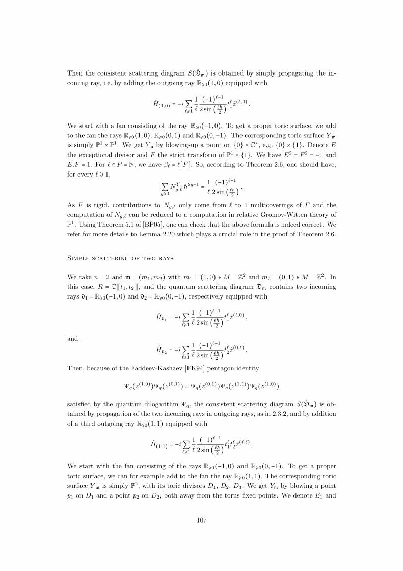
Then the consistent scattering diagram S(Dm) is obtained by simply propagating the in-
coming ray, i.e. by adding the outgoing ray R⩾0(1,0) equipped with
H(1,0) = −i∑`⩾1
1
`
(−1)`−1
2 sin ( `h2)t`1z
(`,0) .
We start with a fan consisting of the ray R⩾0(−1,0). To get a proper toric surface, we add
to the fan the rays R⩾0(1,0), R⩾0(0,1) and R⩾0(0,−1). The corresponding toric surface Y m
is simply P1 × P1. We get Ym by blowing-up a point on 0 ×C∗, e.g. 0 × 1. Denote E
the exceptional divisor and F the strict transform of P1 × 1. We have E2 = F 2 = −1 and
E.F = 1. For ` ∈ P = N, we have β` = `[F ]. So, according to Theorem 2.6, one should have,
for every ` ⩾ 1,
∑g⩾0
NYm
g,` h2g−1
=1
`
(−1)`−1
2 sin ( `h2).
As F is rigid, contributions to Ng,` only come from ` to 1 multicoverings of F and the
computation of Ng,` can be reduced to a computation in relative Gromov-Witten theory of
P1. Using Theorem 5.1 of [BP05], one can check that the above formula is indeed correct. We
refer for more details to Lemma 2.20 which plays a crucial role in the proof of Theorem 2.6.
Simple scattering of two rays
We take n = 2 and m = (m1,m2) with m1 = (1,0) ∈ M = Z2 and m2 = (0,1) ∈ M = Z2. In
this case, R = C[[t1, t2]], and the quantum scattering diagram Dm contains two incoming
rays d1 = R⩾0(−1,0) and d2 = R⩾0(0,−1), respectively equipped with
Hd1 = −i∑`⩾1
1
`
(−1)`−1
2 sin ( `h2)t`1z
(`,0) ,
and
Hd2 = −i∑`⩾1
1
`
(−1)`−1
2 sin ( `h2)t`2z
(0,`) .
Then, because of the Faddeev-Kashaev [FK94] pentagon identity
Ψq(z(1,0)
)Ψq(z(0,1)
) = Ψq(z(0,1)
)Ψq(z(1,1)
)Ψq(z(1,0)
)
satisfied by the quantum dilogarithm Ψq, the consistent scattering diagram S(Dm) is ob-
tained by propagation of the two incoming rays in outgoing rays, as in 2.3.2, and by addition
of a third outgoing ray R⩾0(1,1) equipped with
H(1,1) = −i∑`⩾1
1
`
(−1)`−1
2 sin ( `h2)t`1t
`2z
(`,`) .
We start with the fan consisting of the rays R⩾0(−1,0) and R⩾0(0,−1). To get a proper
toric surface, we can for example add to the fan the ray R⩾0(1,1). The corresponding toric
surface Y m is simply P2, with its toric divisors D1, D2, D3. We get Ym by blowing a point
p1 on D1 and a point p2 on D2, both away from the torus fixed points. We denote E1 and
107

E2 the corresponding exceptional divisors and F the strict transform of the unique line in
P2 passing through p1 and p2. We have E21 = E2
2 = F 2 = −1 and E1.F = E2.F = 1. For ` ∈ Nand (`, `) ∈ P = N2, we have β(`,`) = `[F ]. So according to Theorem 2.6, one should have,
for every ` ⩾ 1,
∑g⩾0
NYm
g,(`,`)h2g−1
=1
`
(−1)`−1
2 sin ( `h2).
As F is rigid, contributions to Ng,(`,`) only come from ` to 1 multicoverings of F and the
computations of Ng,(`,`) reduces to a computation identical to the one used for Ng,` in the
case of trivial scattering.
More complicated scatterings
Already at the classical level of [GPS10], general scattering diagrams can be very compli-
cated. A fortiori, general quantum scattering diagrams are extremely complicated. Direct
computation of the higher genus log Gromov-Witten invariants NYmg,p is a difficult problem
in general. In particular, unlike what happens in the two previously described examples,
linear systems defined by βp and the tangency condition contain in general curves of posi-
tive genus, and so genus g > 0 stable log maps appearing in the moduli space defining NYmg,p
do not factor through genus zero curves in general. As consistent scattering diagrams can
be algorithmically computed, one can view Theorem 2.6 as an answer to the problem of
effectively computing the higher genus log Gromov-Witten invariants NYmg,p .
2.3.3 Orbifold generalization
As in Section 5.5 and 5.6 of [GPS10] for the classical case, we can give an enumera-
tive interpretation of quantum scattering diagrams more general than those considered in
Theorem 2.6 if we allow ourself to work with orbifold Gromov-Witten invariants.
We fix m = (m1, . . . ,mn) an n-tuple of primitive non-zero vectors of M = Z2 and r =
(r1, . . . , rn) an n-tuple of positive integers. We denote P ∶= Nn and we take R ∶= C[[P ]] ∶=
C[[t1, . . . , tn]] as complete local C-algebra. Let Pr be the set of p = (p1, . . . , pn) ∈ P such
that rj divides pj for every 1 ⩽ j ⩽ n. Let Dm,r be the quantum scattering diagram over R
consisting of incoming rays (dj , Hdj), 1 ⩽ j ⩽ n, where
dj = −R⩾0mj ,
and
Hdj = −i∑`⩾1
1
`
(−1)`−1
2 sin (rj`h
2)trj`j zrj`mj =∑
`⩾1
1
`
(−1)`−1
qrj`
2 − q−rj`
2
trj`j zrj`mj ,
where q = eih. Let S(Dm,r) be the corresponding consistent quantum scattering diagram
given by Proposition 2.3, obtained by adding outgoing rays to Dm,r. For every m ∈M −0,
let Pr,m be the subset of p = (p1, . . . , pn) ∈ Pr such that ∑nj=1 pjmj is positively collinear with
m:n
∑j=1
pjmj = `pm
108

for some `p ∈ N.
Recall that in Section 2.2.5, for every m = (m1, . . . ,mn) and r = (r1, . . . , rn), we introduced
an orbifold log Calabi-Yau surface Ym,r and for every p = (p1, . . . , pn) ∈ Pr, we defined some
genus g orbifold log Gromov-Witten NYm,rg,p of Ym,r.
Theorem 2.7. For every m = (m1, . . . ,mn) an n-tuple of primitive non-zero vectors in M ,
every r = (r1, . . . , rn) an n-tuple of positive integers and for every m ∈M −0 primitive, the
Hamiltonian Hm attached to the outgoing ray R⩾0m in the consistent quantum scattering
diagram S(Dm,r) is given by
Hm = (−i
h) ∑p∈Pr,m
⎛
⎝∑g⩾0
NYm,rg,p h2g⎞
⎠
⎛
⎝
n
∏j=1
tpjj
⎞
⎠z`pm .
Remarks:
• For r = (1, . . . ,1), Theorem 2.7 reduces to Theorem 2.6.
• In the classical limit h→ 0, Theorem 2.6 reduces to Theorem 5.6 of [GPS10].
• The proof of Theorem 2.7 is entirely parallel to the proof of its special case Theorem 2.6.
The key point is that orbifold and logarithmic questions never interact in a non-trivial
way. The only major needed modification is an orbifold version of the multicovering
formula of Lemma 2.20. This is done in Lemma 2.25, Section 2.7.2.
2.3.4 More general quantum scattering diagrams
We still fix m = (m1, . . . ,mn) an n-tuple of primitive vectors of M = Z2 and we continue
to denote P = Nn, so that R = C[[P ]] = C[[t1, . . . , tn]]. One could try to further generalize
Theorem 2.7 by starting with a quantum scattering diagram over R consisting of incoming
rays (dj , Hdj), 1 ⩽ j ⩽ n, where dj = −R⩾0mj , and where
Hdj =∑`⩾1
Hdj ,`t`j z`mj ,
for arbitrary
Hdj ,` ∈ C[[h]] .
In the classical limit h → 0, Theorem 5.6 of [GPS10], classical limit of our Theorem 2.7, is
enough to give an enumerative interpretation of the resulting consistent scattering diagram
in such generality. Indeed, the genus zero orbifold Gromov-Witten story takes as input
classical Hamiltonians
Hr =∑`⩾1
(−1)`−1
r`2tr`zr` =
1
r(tz)r +O((tz)r+1
) ,
for all r ⩾ 0, which form a basis of C[(tz)]. In particular, at every finite order in mR, every
classical scattering diagram consisting of n incoming rays meeting at 0 ∈ R2 coincides with a
109

classical scattering diagram whose consistent completion has an enumerative interpretation
in terms of genus zero orbifold Gromov-Witten invariants.
In the quantum story, because of the extra dependence in h, things are more complicated.
Theorem 2.7 only covers a class of Hamiltonians Hdj whose form is dictated by the multi-
covering structure of higher genus orbifold Gromov-Witten theory.
2.4 Gromov-Witten theory of toric surfaces
For every m = (m1, . . . ,mn) an n-tuple of primitive non-zero vectors in M = Z2, we defined
in Section 2.2.1 a log Calabi-Yau surface Ym obtained as blow-up of some toric surface Y m,
and we introduced in Section 2.2.3 a collection of log Gromov-Witten invariants NYmg,p of Ym.
In the present Section, we define analogue log Gromov-Witten invariants NY mg,w of the toric
surface Y m. In the next Section 2.5, we will compare the invariants NYmg,p of Ym and NY m
g,w of
Y m.
2.4.1 Curve classes on toric surfaces
Recall from Section 2.2.1 that Y m is a proper toric surface whose fan contains the rays
−R⩾0mj for j = 1, . . . , n. We denote ∂Y m the union of toric divisors of Y m. We want
to consider curves in Y m meeting ∂Y m in a number of prescribed points with prescribed
tangency conditions and at one unprescribed point with prescribed tangency condition.
In this Section, we explain how to parametrize the relevant curve classes in terms of the
prescribed tangency conditions wj at the prescribed points.
Let s be a positive integer and let w = (w1, . . . ,ws) be a s-tuple of non-zero vectors in M
such that for every r = 1, . . . , s, there exists 1 ⩽ j ⩽ n such that −R⩾0wr = −R⩾0mj . In
particular, the ray −R⩾0wr belongs to the fan of Y m and we denote Dwr the corresponding
toric divisor of Y m. Remark that we can have Dwr =Dwr′ even if r ≠ r′. We denote ∣wr ∣ ∈ Nthe divisibility of wr ∈ M = Z2, i.e. the largest positive integer k such that one can write
wr = kv with v ∈ M . One should think about wr as defining a toric divisor Dwr and an
intersection number ∣wr ∣ with Dwr for a curve in Y m.
We assume that ∑sr=1wr ≠ 0 and so we can uniquely write
s
∑r=1
wr = `wmw ,
with mw ∈M primitive and `w ∈ N.
We explain now how to define a curve class βw ∈ H2(Y m,Z). In short, βw is the class of a
curve in Y m having for every r = 1, . . . , s, an intersection point of intersection number ∣wr ∣
with Dwr , and exactly one other intersection point with the toric boundary ∂Y m.
More precisely, the vector mw ∈M belongs to some cone of the fan of Y m and we write the
corresponding decomposition
mw = aLwmLw + a
Rwm
Rw ,
110

where mLw, mR
w ∈M are primitive generators of rays of the fan of Y m and where aLw, aRw ∈ N.
Remark that there is only one term in this decomposition if the ray R⩾0mw coincides with one
of the rays of the fan of Y m. Let DLw and DR
w be the toric divisors of Y m corresponding to the
rays R⩾0mLw and R⩾0m
Rw. Let βw ∈ H2(Y m,Z) be determined by the following intersection
numbers with the toric divisors:
• Intersection number with Dwr , 1 ⩽ r ⩽ s, distinct from DLw and DR
w :
βw.Dwr = ∑r′,Dwr′ =Dwr
∣wr′ ∣ ,
• Intersection number with DLw:
βw.DLw = `wa
Lw + ∑
r,Dwr=DLw
∣wr ∣ .
• Intersection number with DRw :
βw.DRw = `wa
Rw + ∑
r,Dwr=DRw
∣wr ∣ .
• Intersection number with every toric divisor D different from the Dwr , 1 ⩽ r ⩽ s, and
from DLw and DR
w : βw.D = 0.
Such class βw ∈H2(Y m,Z) exists by standard toric geometry because of the relation
s
∑r=1
wr = `wmw .
2.4.2 Log Gromov-Witten invariant of toric surfaces
In the previous Section, given w = (w1, . . . ,ws) a s-tuple of non-zero vectors in M , we defined
some positive integers `w, aLw, aRw, some toric divisors DLw and DR
w of Y m, and a curve class
βw ∈H2(Y m,Z).
We would like to consider genus g stable map f ∶C → Y m of class βw, intersecting ∂Ym in
s + 1 points, s of them being intersection with Dwr at a point of intersection number ∣wr ∣
for r = 1, . . . , s, and the last one being a point of intersection number `waLw with DL
w and
`waRw with DR
w . We also would like to fix the position of the s intersection numbers with the
divisors Dwr . It is easy to check that the expected dimension of this enumerative problem is
g. As in Section 2.2.3, we will cut down the virtual dimension from g to zero by integration
of the top lambda cass.
As in Section 2.2.3, to get proper moduli spaces, we work with stable log maps. We consider
the divisorial log structure on Y m defined by the toric divisor ∂Y m and use it to view Y m as
a smooth log scheme. Let Mg,w(Y m, ∂Y m) be the moduli space of genus g stable log maps
to Y m, of class βw, with s + 1 tangency conditions along ∂Y m defined by the s + 1 vectors
111

−w1, . . . ,−ws, `wmw in M . It is a proper Deligne-Mumford stack of virtual dimension g + s
and it admits a virtual fundamental class
[Mg,w(Y m, ∂Y m)]virt
∈ Ag+s(Mg,w(Y m, ∂Y m),Q) .
For every r = 1, . . . , s, we have an evaluation map
evr ∶Mg,w(Y m, ∂Y m)→Dwr .
If π∶C → Mg,w(Y m, ∂Y m) is the universal curve, of relative dualizing sheaf ωπ, then the
Hodge bundle E ∶= π∗ωπ is a rank g vector bundle over Mg,w(Y m, ∂Y m), of top Chern class
λg ∶= cg(E).
We define
NY mg,w ∶= ∫
[Mg,w(Y m,∂Y m)]virt(−1)gλg
s
∏r=1
ev∗r(ptr) ∈ Q ,
where ptr ∈ A1(Dwi) is the class of a point. It is a rigorous definition of the enumerative
problem sketched at the beginning of this Section.
2.5 Degeneration from log Calabi-Yau to toric
2.5.1 Degeneration formula: statement
We fix m = (m1, . . . ,mn) an n-tuple of primitive non-zero vectors inM = Z2. In Section 2.2.1,
we defined a log Calabi-Yau surface Ym obtained as blow-up of some toric surface Y m.
In Section 2.2.3, we introduced a collection of log Gromov-Witten invariants NYmg,p of Ym,
indexed by n-tuples p = (p1, . . . , pn) ∈ P = Nn. In Section 2.4.2, we defined log Gromov-
Witten invariants NY mg,w of the toric surface Y m indexed by s-tuples w = (w1, . . . ,ws) ∈M
s.
The main result of the present Section, Proposition 2.8, is the statement of an explicit
formula expressing the invariants NYmg,p in terms of the invariants NY m
g,p .
We first need to introduce some notations to relate the indices p = (p1, . . . , pn) indexing the
invariants NYmg,p and the indices w = (w1, . . . ,ws) indexing the invariants NY m
g,w . The way it
goes is imposed by the degeneration formula in Gromov-Witten theory and hopefully will
become conceptually clear in Section 2.5.4.
We fix p = (p1, . . . , pn) ∈ P = Nn. We call k a partition of p, and we write k ⊢ p, if k is an
n-tuple (k1, . . . , kn), with kj a partition of pj , for 1 ⩽ j ⩽ n. We encode a partition kj of pj
as a sequence kj = (k`j)`⩾1 of non-negative integers, all zero except finitely many of them,
such that
∑`⩾1
`k`j = pj .
Given k a partition of p, we denote
s(k) ∶=n
∑j=1
∑`⩾1
k`j .
112

We now define, given a partition k of p, a s(k)-tuple
w(k) = (w1(k), . . . ,ws(k)(k))
of non-zero vectors in M = Z2, by the following formula:
wr(k) ∶= `mj
if
1 +j
∑j′=1
`−1
∑`′=1
k`′j′ ⩽ r ⩽ k`j +j
∑j′=1
`−1
∑`′=1
k`′j′ .
In particular, for every 1 ⩽ j ⩽ n and ` ⩾ 1, the s(k)-tuple w(k) contains k`j copies of the
vector `mj ∈ M . Remark that because mj is primitive in M , we have ` = ∣wr(k)∣, where
∣wr(k)∣ is the divisibility of wr(k) in M . Remark also that
s(k)
∑r=1
wr(k) =n
∑j=1
∑`⩾1
k`j`mj =n
∑j=1
pjmj = `pmp ,
and so, comparing notations of Sections 2.2.2 and 2.4.1, `w(k) = `p and mw(k) =mp.
Using the above notations, we can now state Proposition 2.8.
Proposition 2.8. For evey m = (m1, . . . ,mn) an n-tuple of primitive non-zero vectors in
M = Z2, and for every p = (p1, . . . , pn) ∈ P = Nn, the log Gromov-Witten invariants NYmg,p of
the log Calabi-Yau surface Ym are expressed in terms of the log Gromov-Witten invariants
NY mg,w of the toric surface Y m by the following formula:
∑g⩾0
NYmg,p h
2g−1
= ∑k⊢p
⎛
⎝∑g⩾0
NY m
g,w(k)h2g−1+s(k)⎞
⎠
n
∏j=1
∏`⩾1
1
k`j !`k`j
⎛
⎝
(−1)`−1
`
1
2 sin ( `h2)
⎞
⎠
k`j
,
where the first sum is over all partitions k of p.
The proof of Proposition 2.8 takes Sections 2.5.2, 2.5.3, 2.5.4, 2.5.5, 2.5.6. We consider the
degeneration from Ym to Y m introduced in Section 5.3 of [GPS10] and we apply a higher
genus version of the argument of [GPS10]. Because the general degeneration formula in
log Gromov-Witten theory is not yet available, we give a proof of the needed degeneration
formula following the general strategy used in Chapter 1, which uses specific vanishing
properties of the top lambda class.
2.5.2 Degeneration set-up
We first review the construction of the degeneration considered in Section 5.3 of [GPS10].
We fix m = (m1, . . . ,mn) an n-tuple of primitive non-zero vectors in M = Z2. Recall from
Section 2.2.1 that Y m is a proper toric surface whose fan contains the rays −R⩾0mj for
113

j = 1, . . . , n, and that we denote Dmj the corresponding toric divisors. For every j = 1, . . . , n,
we also choose a point xj in general position on the toric divisor Dmj . Let Y m ×C → C be
the trivial family over C and let xj ×C be the sections determined by the points xj . Up
to doing some toric blow-ups, which do not change the log Gromov-Witten invariants we
are considering by [AW13], we can assume that the divisors Dmj are disjoint.
The degeneration of Y m to the normal cone of Dm1 ∪ ⋅ ⋅ ⋅ ∪Dmn ,
εYm
∶Ym → C ,
is obtained by blowing-up the loci Dm1 , . . . ,Dmn over 0 ∈ C in Y m ×C. The special fiber is
given by
ε−1Ym
(0) = Y m ∪n
⋃j=1
Pj ,
where NDmj ∣Y mis the normal line bundle to Dmj in Y m, and Pj is the projective bundle over
Dmj obtained by projectivization of the rank two vector bundle ODmj ⊕NDmj ∣Y mover Dmj .
The embeddings ODmj ODmj ⊕NDmj ∣Y mand NDmj ∣Y m
ODmj ⊕NDmj ∣Y minduce two
sections of Pj →Dmj that we denote respectively Dmj ,∞ and Dmj ,0. In ε−1Ym
(0), the divisor
Dmj in Y m is glued to the divisor Dmj ,0 in Pj . The strict transform of the section xj×Cof Y m ×C is a section Sj of ε
Ym, whose intersection with ε−1
Ym(0) is a point xj,∞ ∈Dmj ,∞.
We then blow-up the sections Sj , j = 1, . . . , n, in Ym and we obtain a family
εYm∶Ym → C, .
whose fibers away from zero are isomorphic to the surface Ym, and whose special fiber is
given by
Ym,0 ∶= ε−1Ym
(0) = Y m ∪n
⋃j=1
Pj ,
where Pj is the blow-up of Pj at all the points xj′,∞ such that Pj′ = Pj . We denote Ej′
the corresponding exceptional divisor in Pj and Cj′ the strict transform in Pj of the unique
P1-fiber of Pj →Dmj containing xj′,∞. We have Ej′ .Cj′ = 1 in Pj .
We would like to get Proposition 2.8 by application of a degeneration formula in log Gromov-
Witten theory to the family
εYm∶Ym → C ,
to relate the invariants NYmg,p of the general fiber Ym to the invariants NY m
g,w of Y m which
appears as component of the special fiber Ym,0. In [GPS10], Gross-Pandharipande-Siebert
work with an ad hoc definition of the genus 0 invariants as relative Gromov-Witten invariants
of some open geometry and they only need to apply the usual degeneration formula in
relative Gromov-Witten theory. In our present setting, with log Gromov-Witten invariants
in arbitrary genus, we cannot follow exactly the same path.
Because the general degeneration formula in log Gromov-Witten theory is not yet avail-
able, we follow the strategy used in Chapter 1. We apply the decomposition formula
of Abramovich-Chen-Gross-Siebert [ACGS17a], we use the vanishing property of the top
114

lambda class to restrict the terms appearing in this formula and to prove a gluing formula
by working only with torically transverse stable log maps. We review the decomposition
formula of [ACGS17a] in Section 2.5.3. In Section 2.5.4, we identify the various terms
contributing to the decomposition formula. In Section 2.5.5, we prove a gluing formula
computing each of these terms. We finish the proof of Proposition 2.8 in Section 2.5.6.
2.5.3 Statement of the decomposition formula
We consider Ym as a smooth log scheme for the divisorial log structure defined by the
divisor Ym,0 union the strict transforms of the divisors ∂Y m ×C in Y m ×C for j = 1, . . . , n.
Considering C as a smooth log scheme for the divisorial log structure defined by the divisor
0, we get that εYmis a log smooth morphism. Restricting to the special fiber gives a
structure of log scheme on Ym,0 and a log smooth morphism to the standard log point ptN(the point 0 equipped with the log structure restricted by 0 C of the divisorial log
structure on C):
εYm,0 ∶Ym,0 → ptN .
Let Mg,p(Ym,0) be the moduli space of genus g stable log maps to εYm,0 ∶Ym,0 → ptN, of class
βp, with a marked point of contact order `pmp. It is a proper Deligne-Mumford stack of
virtual dimension g and it admits a virtual fundamental class
[Mg,p(Ym,0)]virt
∈ Ag(Mg,p(Ym,0),Q) .
By deformation invariance of the virtual fundamental class on moduli spaces of stable log
maps in log smooth families, we have
NYmg,p = ∫
[Mg,p(Ym,0)]virt(−1)gλg .
The decomposition formula of [ACGS17a] gives a decomposition of [Mg,p(Ym,0)]virt indexed
by tropical curves mapping to the tropicalization of Ym,0. These tropical curves encode the
intersection patterns of irreducible components of stable log maps mapping to the special
fiber of the degeneration. We refer to Appendix B of [GS13] and Section 2 of [ACGS17a] for
the general notion of tropicalization of a log scheme. We denote Σ(X) the tropicalization
of a log scheme X, it is a cone complex, i.e. an abstract gluing of cones.
We start by describing the tropicalization Σ(Ym,0) of Ym,0. Tropicalizing the log mor-
phism εYm,0 ∶Ym,0 → ptN, we get a morphism of cone complexes Σ(εYm,0)∶Σ(Ym,0)→ Σ(ptN).
We have Σ(ptN) = R⩾0 and Σ(Ym,0) is naturally identified with the cone over the fiber
Σ(εYm,0)−1(1) at 1 ∈ R⩾0. It is thus enough to describe the cone complex Σ(εYm,0)
−1(1). We
denote
Ytropm,0 ∶= Σ(εYm,0)
−1(1) .
The cone complex Ytropm,0 is the tropicalization of
Ym,0 = Y m ∪n
⋃j=1
Pj ,
115

equipped with the divisorial log structure defined by the divisor ∂Y m ∪ ⋃nj=1 ∂Pj . In par-
ticular, it has one vertex v0 dual to Y m and vertices vj dual to Pj , j = 1, . . . , n. For every
j = 1, . . . , n, there is an edge ej,0 of integral length 1, connecting v0 and vj , dual to Dmj ,0,
and an unbounded edge ej,∞ attached to vj , dual to Dmj ,∞.
The best way to understand Ytropm,0 is probably to think about it as a modification of the
tropicalization of Y m. As Y m is simply a toric surface, its tropicalization Σ(Y m) can be
naturally identified with R2 endowed with the fan decomposition. In particular, Σ(Y m)
has one vertex v0 = 0 ∈ R2 and unbounded edges −R⩾0mj , attached to v0 and dual to the
toric boundary divisors Dmj . To go from Σ(Y m) to Ytropm,0 , one adds a vertex vj on each
primitive integral point of −R⩾mj , which has the effect to split −R⩾0vj into a bounded edge
ej,0 and an unbounded edge ej,∞. One still has to cut along ej,∞ and to insert there two
two-dimensional cones dual to the two “corners” of ∂Pj which are on Dmj ,∞. In particular,
for j = 1, . . . , n, the vertex vj is 4-valent and looks locally as the fan of the Hirzebruch surface
Pj . In general, there is no global linear embedding of Ytropm,0 in R2.
r
HHH
HHH
HHH
HHH
AAAAAAAAA
−R⩾0m10
−R⩾0m2
Figure: tropicalization of Y m.
r
HHHH
HHH
HHH
HH
AAAAAAAAA
r
AAAAAA
r
v0 e1,0 e1,∞
v1
v2
e2,0
e2,∞
Figure: picture of Ytropm,0 .
116

We refer to Definition 2.5.3 of [ACGS17a] for the general definition of parametrized tropical
curve h∶Σ → Ytropm,0 . It is a natural generalization of the notion of parametrized tropical
curve in R2 that we will use and review in Section 2.6.1. In particular, Σ is a graph, with
bounded and unbounded edges mapped by h to Ytropm,0 in an affine linear way and vertices
V of Σ are decorated by some genus g(V ). The total genus g of the parametrized tropical
curve is defined by gΓ +∑V g(V ), where gΓ is the genus of the graph Γ.
Some distinction between Ytropm,0 and R2, related to the fact that the components Pj of Ym,0
are non-toric, is that the usual form of the balancing condition for tropical curve in R2 is
not necessarily valid at vertices of Γ mapping to one of the vertices vj , j = 1, . . . , n, of Ytropm,0 .
For vertices of Γ mapping away from vj , j = 1, . . . , n, the usual balancing condition applies.
Following Definition 4.2.1 of [ACGS17a], a decorated parametrized tropical curve is a
parametrized tropical curve h∶Γ → Ytropm,0 where each vertex has a further decoration by
a curve class in the stratum of Ym,0 dual to the stratum of Ytropm,0 where this vertex is
mapped. In short, a decorated parametrized tropical curve to Ytropm,0 encodes all the neces-
sary combinatorial information to be a fiber of the tropicalization of a stable log maps to
Ym,0.
The decomposition formula of [ACGS17a] involves decorated parametrized tropical curves
which are rigid in their combinatorial type. This is easy to understand intuitively: the
decomposition formula is supposed to describe how the moduli space of stable log maps
breaks into pieces under degeneration. If the moduli space of tropical curves were the trop-
icalization, and so the dual intersection complex, of the moduli space of stable log maps,
components of the moduli space of stable log maps should be in bijection with the zero
dimensional strata of the moduli space of tropical curves, i.e. with exactly rigid tropical
curves. The decomposition formula [ACGS17a] expresses that this intuitive picture is cor-
rect, at least at the virtual level.
The tropical curves relevant in the study of Mg,p(Ym,0) are genus g decorated parametrized
tropical curve Γ → Ytropm,0 of type p, i.e. with only one unbounded edge, of weight `p and of
direction mp, and with total curve class βp.
According to Section 4.4 of [ACGS17a], for every h∶Γ → Ytropm,0 rigid genus g decorated
parametrized topical curve of type p, there exists a notion of stable log map marked by h,
and a moduli space Ym,0 → ptN of stable log maps marked by h, which is a proper Deligne-
Mumford stack equipped with a virtual fundamental class [Mhkg,p(Ym,0)]
virt. Forgetting the
marking by h gives a morphism
ih∶Mh
g,p(Ym,0)→Mh
g,p(Ym,0) .
We can finally state the decomposition formula, Theorem 4.8.1 of [ACGS17a]: we have
[Mg,p(Ym,0)]virt
=∑h
nh∣Aut(h)∣
(ih)∗[Mh
g,p(Ym,0)]virt ,
where the sum is over rigid genus g decorated parametrized tropical curves h∶Γ → Ytropm,0
of type p, nh is the smallest positive integer such that after scaling by nh, h gets integral
117

vertices and integral lengths, and ∣Aut(h)∣ is the order of the automorphism group of h.
2.5.4 Classification of rigid tropical curves
In order to extract some explicit information from the decomposition formula, the first step
is to identify the rigid decorated parametrized tropical curves h∶Γ → Ytropm,0 of type p. It is
in general a difficult question. But because we are only interested in invariants obtained
by integration of the top lambda class λg, and not in the full virtual class, the situation is
much simpler by the following Lemma.
Lemma 2.9. Let h∶Γ → Ytropm,0 be a genus g rigid decorated parametrized tropical curve of
type p with Γ of positive genus. Then we have
∫[M
h
g,p(Ym,0)]virt(−1)gλg = 0 .
Proof. If f ∶C → Ytropm,0 is a stable log map in M
h
g,p(Ym,0), then, by definition of the marking
by h, the dual intersection complex of C retracts onto Γ and in particular, has genus bigger
than the genus of Γ, which is positive by hypothesis. It follows that C contains a cycle of
irreducible components. By Lemma 1.7, the class λg vanishes on families of curves containing
cycles of irreducible components.
By Lemma 2.9, we only have to determine the rigid decorated parametrized tropical curves
h∶Γ→ Ytropm,0 of type p with Γ of genus zero.
Recall that we defined in Section 2.5.1 what is a partition of p and that we associated to
such partition k of p a positive integer s(k) and a s(k)-tuple (w1, . . . ,ws(k)) of non-zero
vectors in M = Z2. In particular, each wr(k) can be naturally written wr(k) = `mj for some
` ⩾ 0 and some 1 ⩽ j ⩽ n.
We first explain how to construct a genus g rigid decorated parametrized tropical curve
hk,g ∶Γk,g → Ytropm,0 with Γk,g of genus zero, for every partition k of p and for every g =
(g0, g1, . . . , gs(k)), (s(k) + 1)-tuple of non-negative integers such that ∣g∣ ∶= g0 + ∑s(k)r=1 gr =
g. We refer to Section 2.5 of [ACGS17a] for details on the general notion of decorated
parametrized tropical curve.
Let Γk,g be the genus zero graph6 consisting of vertices V0, V1, . . . , Vs(k), bounded edges Er,
r = 1, . . . , s(k), connecting V0 to Vr, and an unbounded edge Ep attached to V0.
We define a structure of tropical curve on Γk,g by assigning:
• Genera to the vertices. We assign g0 to V0, and gr to Vr, for all 1 ⩽ r ⩽ s(k).
• Lengths to the bounded edges. We assign the length
`(Er) ∶=1
∣wr(k)∣=
1
`
6We assume for simplicity that mp does not coincide with any of the −mj . If not, we need to add a2-valent vertex Vp on Ep and we have hk,g(Vp) = vj for j such that mp = −mj .
118

to the bounded edge Er, for all 1 ⩽ r ⩽ s(k).
Finally, we define a decorated parametrized tropical curve
hk,g ∶Γk,g → Ytropm,0
by the following data:
• We define hk,g(V0) ∶= v0, and, writing wr(k) = lmj , hk,g(Vr) ∶= vj , for all 1 ⩽ r ⩽ s(k).
• Edge markings of bounded edges. We define vV0,Er ∶= wr for all 1 ⩽ r ⩽ s(k). In
particular, the bounded edge Er has weight ∣wr(k)∣ = `. This is a valid choice because
h(Vr) − h(V0) =mj =1
``mj = `(Er)vV0,Er .
This uniquely specifies an affine linear map hk,g ∣Er .
• Edge marking of the unbounded edge. We define vV0,Ep ∶= `pmp. In particular, the
unbounded edge Ep has weight `p. This uniquely specifies an affine linear map hk,g ∣Ep .
• Decoration of vertices by curve classes. We decorate V0 with the curve class βw(k) ∈
H2(Y m,Z). Writing wr(k) = `mj , we decorate the vertex Vr with the curve class
`[Cj] ∈H2(Pj ,Z).
Figure: picture of Γk,g.
r
HHH
HHH
AAAAAAAAA
rr
rV2
E2
V0 E1 V1
V3
E3
Ep
Lemma 2.10. The genus g decorated parametrized tropical curve
hk,g ∶Γk,g → Ytropm,0
is rigid.
Proof. This is obvious because hk,g has no contracted edge and all vertices of Γk,g are mapped
to vertices of Ytropm,0 : it is not possible to deform hk,g without changing its combinatorial
type.
119

Proposition 2.11. Every genus g rigid decorated parametrized tropical curve h∶Γ → Ytropm,0
of type p, with Γ of genus zero, is of the form hk,g for some k partition of p and g =
(g0, g1, . . . , gs(k)) some (s(k) + 1)-tuple of non-negative integers such that ∣g∣ = g.
Proof. The argument7 is similar to the one used in the proof of Proposition 1.10, itself
a tropical version of the properness argument, Proposition 4.2, of [GPS10]. By iterative
application of the balancing condition, we will argue that the source Γ of a rigid decorated
parametrized tropical curve h∶Γ→ Ytropm,0 of type p not of the form hk,g, necessarily contains
a closed cycle and so has positive genus.
Let h∶Γ → Ytropm,0 be a genus g rigid parametrized tropical curve of type p. As h is rigid,
there is no edge of Γ contracted by h. The fact that h has type p implies that h has only
one unbounded edge and this unbounded edge has weight `p and direction mp.
Lemma 2.12. Assume that there exists a vertex V of Γ such that
h(V ) ∉ v0, v1, . . . , vn ,
then Γ has positive genus.
Proof. We first assume that h(V ) is contained in the interior of one of the two-dimensional
cones C of Ytropm,0 . Because h(V ) is away from the vertices vj , the situation is locally toric
and the balancing condition has to be satisfied in h(V ). If h(V ) ∉ R⩾0mp, there is no
unbounded edge of Γ ending at V , and so by balancing, not all edges attached to h(V ) can
point towards the vertex of C, i.e. at least one edge of C points towards a boundary ray of
C. If h(V ) ∈ R⩾0mp, we can get the same conclusion: if all edges passing through h(V )
were parallel to R⩾0mp, this would contradict the rigidity of h because one could move h(V )
along R⩾0mp.
Then, we follow the proof of Proposition 1.10. Fixing a cyclic orientation on the collection
of cones and rays of Ytropm,0 , we can assume that this edge points towards the left (from the
point of view of the vertex of the cone, looking inside the cone) ray of C. If this edge ends on
some vertex still contained in the interior of C, then the balancing condition still applies and
so there is still an edge attached to this vertex pointing towards the left ray of C. Because
Γ has finitely many vertices, iterating this construction finitely many times, we construct a
path starting from h(V ) and ending at some vertex h(V ′) on the left boundary ray of C.
Let C′ be the two-dimensional cone of Ytropm,0 adjacent to C near h(V ′). Then we claim that
by the balancing condition, there exists an edge attached to h(V ′) pointing towards the left
ray of C′. Indeed, the only case for which the balancing condition is not a priori satisfied is
if h(V ′) = vj for some j. But at vj , the non-toric nature of Pj only modifies the balancing
condition in the direction parallel to ej,0 and ej,∞: if there is an incoming edge with non-zero
transversal direction, then there is still an outgoing edge with non-zero transversal direction
(Pj is obtained from the Hirzebruch surface Pj →Dmj by blowing-up points on the divisors
7We assume for simplicity that mp is distinct from all −mj . It is easy to adapt the argument in thisspecial case.
120

Dmj ,∞: this does not affect the fact that the general fibers of Pj → Dmj are still linearly
equivalent).
Iterating this construction, we get a path in Γ whose image by h in Ytropm,0 is a path which
intersects successive rays in the anticlockwise order. Because Γ has finitely many edges, this
path has to close eventually and so Γ contains a non-trivial closed cycle, i.e. Γ has positive
genus.
It remains to treat the case where h(V ) is in the interior of a one dimensional ray of Ytropm,0 .
If all the edges attached to h(V ) were parallel to the ray, this would contradict the ridigity
of h because one could move h(V ) along the ray. So at least one of the edges attached
to h(V ) is not parallel to the ray and by balancing, we can assume that there is an edge
attached to h(V ) pointing towards the 2-dimensional cone of Ytropm,0 left to the ray. We can
then apply the iterative argument described above.
We continue the proof of Proposition 2.11. Let us assume that Γ has genus zero. By
Lemma 2.12, every vertex V of Γ maps to one of the vertices v0, v1, . . . , vn of Γ. If there
were an edge connecting a vertex mapped to vj with a vertex mapped to vj′ , 1 ⩽ j, j′ ⩽ n
with j ≠ j′, then we could apply the iterative argument used in the proof of Lemma 2.12,
and this would contradict the assumption that Γ has genus zero.
It follows that every edge in Γ adjacent to some vertex mapped to vj for some 1 ⩽ j ⩽ n is
also adjacent to some vertex mapped to v0. As Γ is connected and there is no contracted
edges, this implies that there is a unique vertex V0 of Γ such that h(V0) = v0. As Γ is of type
p, the curve classes of the vertices mapping to vj , 1 ⩽ j ⩽ n, naturally define a partition k of
p, the genera of the various vertices define some g and it is easy to check that h = hk,g.
Define
Nhk,gg,p ∶= ∫
[Mhk,gg,p (Ym,0)]virt
(−1)gλg ∈ Q .
Proposition 2.13. We have
NYmg,p = ∑
k⊢p
∑g
∣g∣=g
nhk,g∣Aut(hk,g)∣
Nhk,gg,p .
Proof. This follows from integrating (−1)gλg over the decomposition formula of [ACGS17a],
reviewed at the end of Section 2.5.3. By Lemma 2.9, rigid tropical curves h∶Γ→ Ytropm,0 , with
Γ of positive genus, do not contribute, and by Proposition 2.11, all the relevant rigid tropical
curves h∶Γ → Ytropm,0 are of the form hk,g ∶Γk,g → Y
tropm,0 for some k partition of p and some g
such that ∣g∣ = g.
We fix k a partition of p and g such that ∣g∣ = g and we consider the decorated parametrized
tropical curve h∶Γk,g → Ytropm,0 .
Lemma 2.14. We have
nhk,g = lcm∣wr(k)∣,1 ⩽ r ⩽ s(k) .
121

Proof. Recall that nhk,g is the smallest positive integer such that after scaling by nkk,g , hk,g
gets integral vertices and integral lengths. By definition of hk,g, vertices of hk,g are already
mapped to integral points of Ytropm,0 . On the other hand, bounded edges Er of Γk,g have
fractional lengths 1/∣wr(k)∣. It follows that nk,g is the least common multiple of the positive
integers ∣wr(k)∣, 1 ⩽ r ⩽ s(k).
For 1 ⩽ j ⩽ n, ` ⩾ 1 and a ⩾ 0, denote k`ja the number of vertices of Γk,g having genus a
among the k`j ones having curve class decoration `[Cj]. Remark that we have
k`j = ∑a⩾0
k`ja ,
ands(k)
∑r=1
gr =n
∑j=1
∑`⩾1
∑a⩾0
ak`ja .
Lemma 2.15. The order of the automorphism group of the decorated parametrized tropical
curve hk,g ∶Γk,g → Ytropm,0 is given by
∣Aut(hk,g)∣ =n
∏j=1
∏`⩾1
∏a⩾0
k`ja! .
Proof. For every 1 ⩽ j ⩽ n, ` ⩾ 1 and a ⩾ 0, there are k`ja of the vertices Vr having the
same curve class decoration `[Cj], the same genus a, and the attached edges have the same
weight ellmj , so permutations of these k`ja vertices define automorphisms of the decorated
tropical curve hk,g. Any other permutation of the vertices of Σk permutes vertices having
different curve class decorations and/or different genus, and so cannot be an automorphism
of the decorated tropical curve.
Corollary 2.16. We have
NYmg,p = ∑
k⊢p
∑g
∣g∣=g
(lcm∣wr(k)∣,1 ⩽ r ⩽ s(k))⎛
⎝
n
∏j=1
∏`⩾1
∏a⩾0
1
k`ja!
⎞
⎠Nhk,gg,p .
Proof. Combination of Proposition 2.13, Lemma 2.14 and Lemma 2.15.
2.5.5 Gluing formula
The previous Section has reduced the computation of the log Gromov-Witten invariants
NYmg,p to the computation of invariants
Nhk,gg,p ∶= ∫
[Mhk,gg,p (Ym,0)]virt
(−1)gλg .
where Mhk,gg,p (Ym,0) is a moduli space of stable log maps to Ym,0 marked by hk,g, i.e. whose
tropicalization is equipped with a retraction on hk,g.
122

Let f ∶C → Ym,0 be a stable log map of tropicalization hk,g. Then C has irreducible compo-
nents C0,C1, . . . ,Cs(k), of genus g0, g1, . . . , gs(k) and we have
• f ∣C0 is a genus g0 stable map to Y m of class βw(k), transverse to ∂Y m, with s + 1
tangency conditions along ∂Y m defined by the s + 1 vectors −w1, . . . ,−ws, `pmp ∈M8.
• For all 1 ⩽ r ⩽ s(k), wr(k) = lmj , f ∣Cr is a genus gr stable map to Pj , of class `[Cj],
with a full tangency condition of order ` along Dmj ,0.
This suggests to consider the moduli space Ma,`(Pj , ∂Pj) of genus a stable log maps to Pj ,equipped with the divisorial log structure with respect to the divisor ∂Pj , of class `[Cj],
with a full tangency condition of order ` along Dmj . It is a proper Deligne-Mumford stack
of virtual dimension a, admitting a virtual fundamental class
[Ma,`(Pj , ∂Pj)]virt∈ Aa(Ma,`(Pj , ∂Pj),Q) .
We define
N `Pja ∶= ∫
[Ma,`(Pj ,∂Pj)]virt(−1)aλa ∈ Q .
The decomposition of a stable log map f ∶C → Ym,0 into irreducible components suggests
that we should be able to express Nhk,gg,p in terms of NY m
g0,w(k)and N
`Pja .
The following Proposition 2.17 gives a gluing formula showing that it is indeed the case.
Proposition 2.17. We have
Nhk,gg,p =
NY m
g0,w(k)
lcm∣wr(k)∣,1 ⩽ r ⩽ s(k)
⎛
⎝
n
∏j=1
∏`⩾1
`k`j ∏a⩾0
(N `Pja )
k`ja⎞
⎠.
Proof. We gave a brief description of stable log maps whose tropicalization is hk,g as a
motivation for why a gluing formula like Proposition 2.17 should be true. But the moduli
space of such stable log maps is not proper. The relevant proper moduli space Mhk,gg,p (Ym,0)
is a moduli space of stable log maps marked by hk,g, containing stable log maps whose
tropicalization only retracts onto hk,g. These stable log maps interact in a complicated way
with the log structure of Ym,0 and the gluing of such stable log maps has not been worked
out yet.
We go around this issue by following the strategy used in Section 1.6. On an open locus
of torically transverse stable maps, the above mentioned problems do not arise and the
difficulty of the gluing problem is of the same level as the usual degeneration formula in
relative Gromov-Witten theory. The log version of this gluing problem has been recently
treated in full details by Kim, Lho and Ruddat [KLR18]. On the complement of the nice
locus of torically transverse stable log maps, a combinatorial argument of Proposition 1.10
implies that one of the relevant curves will always contain a non-trivial cycle of components.
8For simplicity, we are assuming that mp is distinct from all −mj . It is easy to adapt the argument inthis special case. The gluing formula remains unchanged, for the same reason that 2-valent vertices play atrivial role in Chapter 1: see Lemma 1.14.
123
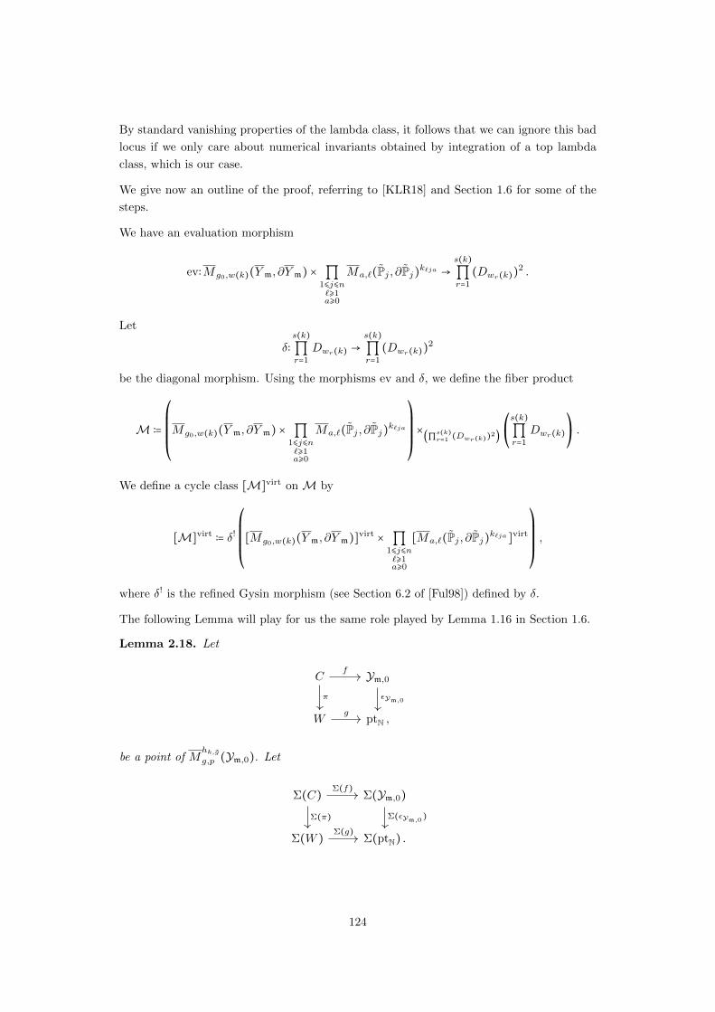
By standard vanishing properties of the lambda class, it follows that we can ignore this bad
locus if we only care about numerical invariants obtained by integration of a top lambda
class, which is our case.
We give now an outline of the proof, referring to [KLR18] and Section 1.6 for some of the
steps.
We have an evaluation morphism
ev∶Mg0,w(k)(Y m, ∂Y m) × ∏1⩽j⩽n`⩾1a⩾0
Ma,`(Pj , ∂Pj)k`ja →s(k)
∏r=1
(Dwr(k))2 .
Let
δ∶s(k)
∏r=1
Dwr(k) →
s(k)
∏r=1
(Dwr(k))2
be the diagonal morphism. Using the morphisms ev and δ, we define the fiber product
M ∶=
⎛⎜⎜⎜⎜⎝
Mg0,w(k)(Y m, ∂Y m) × ∏1⩽j⩽n`⩾1a⩾0
Ma,`(Pj , ∂Pj)k`ja⎞⎟⎟⎟⎟⎠
×(∏
s(k)r=1 (Dwr(k))
2)
⎛
⎝
s(k)
∏r=1
Dwr(k)
⎞
⎠.
We define a cycle class [M]virt on M by
[M]virt ∶= δ!
⎛⎜⎜⎜⎜⎝
[Mg0,w(k)(Y m, ∂Y m)]virt
× ∏1⩽j⩽n`⩾1a⩾0
[Ma,`(Pj , ∂Pj)k`ja]virt
⎞⎟⎟⎟⎟⎠
,
where δ! is the refined Gysin morphism (see Section 6.2 of [Ful98]) defined by δ.
The following Lemma will play for us the same role played by Lemma 1.16 in Section 1.6.
Lemma 2.18. Let
C Ym,0
W ptN ,
f
π εYm,0
g
be a point of Mhk,gg,p (Ym,0). Let
Σ(C) Σ(Ym,0)
Σ(W ) Σ(ptN) .
Σ(f)
Σ(π) Σ(εYm,0)
Σ(g)
124

be its tropicalization. For every b ∈ Σ(g)−1(1), let
Σ(f)b∶Σ(C)b → Σ(εYm,0)−1
(1) = Ytropm,0
be the fiber of Σ(f) over b. For every r = 1, . . . , s(k), let EΣ(f)br be the edge of Σ(f)b marked
by the edge Er of Γk,g. Then, we have
h(EΣ(f)br ) ⊂ hk,g(Er) .
Proof. This follows from the fact that for every 1 ⩽ j ⩽ n, the curve Cj is rigid in Pj , so the
vertices of Γ marked by the vertex Vr of Γk,g are mapped on hk,g(Er).
Given a stable log map f ∶C → Ym,0 marked by hk,g, we have nodes of C in correspondence
with the bounded edges of Γ. Cutting C along these nodes, we obtain a morphism
cut∶Mhk,gg,p (Ym/∂Ym)→M .
Because of Lemma 2.18, each cut is locally identical to the corresponding cut in a degener-
ation along a smooth divisor and so we can refer to Section 1.6 or Section 5 of [KLR18] for
a precise definition of the cut morphism, dealing with log structures.
We say that a stable log map f ∶C → Y m is torically transverse if its image does not contain
any of the torus fixed points of Y m, i.e. if its image does not pass through the “corners”
of the toric boundary divisor ∂Y m, i.e. if its tropicalization has no vertex mapping in the
interior of one of the two-dimensional cones of the fan of Y m.
Let M0
g0,w(k)(Y m, ∂Y m) be the open substack of Mg0,w(k)(Y m, ∂Y m) consisting of torically
transverse stable log maps. We define
M0 ∶=
⎛⎜⎜⎜⎜⎝
M0
g0,w(k)(Y m, ∂Y m) × ∏1⩽j⩽n`⩾1a⩾0
Ma,`(Pj , ∂Pj)k`ja⎞⎟⎟⎟⎟⎠
×(∏
s(k)r=1 (Dwr(k))
2)
⎛
⎝
s(k)
∏r=1
Dwr(k)
⎞
⎠,
Mhk,g,0
g,p (Ym/∂Ym) ∶= cut−1(M
0) ,
and we denote
cut0∶M
hk,g,0
g,p (Ym/∂Ym)→M0
the corresponding restriction of the cut morphism.
Lemma 2.19. The morphism
cut0∶M
hk,g,0
g,p (Ym/∂Ym)→M0
is etale of degree∏nj=1∏`⩾1 `
k`j
lcm∣wr(k)∣,1 ⩽ r ⩽ s(k).
125

Proof. Because of the restriction to the torically transverse locus, the gluing question is
locally isomorphic to the corresponding gluing question in a degeneration along a smooth
divisor, and so the result follows from formula (6.13) and Lemma 9.2 of [KLR18]9.
Restricted to the torically transverse locus, the comparison of obstruction theories on
Mhk,gg,p (Ym/∂Ym) and M reduces to the same question studied in Section 9 of[KLR18] for
a degeneration along a smooth divisor. In particular, combining Lemma 2.19 with formula
9.14 of [KLR18], we obtain that the cycle classes
(cut)∗([Mhk,gg,p (Ym/∂Ym)]
virt)
and∏nj=1∏`⩾1 `
k`j
lcm∣wr(k)∣,1 ⩽ r ⩽ s(k)[M]
virt
have the same restriction to the open substackM0 ofM. It follows by [Ful98] Proposition 1.8,
that their difference is rationally equivalent to a cycle supported on the closed substack
Z ∶=M −M0 .
At a point of Z, the corresponding stable log map f ∶C → Y m to Y m is not torically transverse.
Using Lemma 2.18, we can apply Proposition 1.10 to get that C contains a non-trivial cycle
of components. Vanishing properties of lambda classes given by Lemma 1.7, combined with
gluing properties of lambda classes given by Lemma 1.6, finally imply the gluing formula
stated in Proposition 2.17, as in the end of Section 1.6.
Remark: The most general form of the gluing formula in log Gromov-Witten theory, work in
progress of Abramovich-Chen-Gross-Siebert, requires the use of punctured Gromov-Witten
invariants, see [ACGS17b]. We do not see punctured invariants in our gluing formula because
we only consider rigid tropical curves contained in the polyhedral decomposition of Ytropm,0 .
2.5.6 End of the proof of the degeneration formula
We now finish the proof of the degeneration formula, Proposition 2.8.
Combining Corollary 2.16 with Proposition 2.17, we get
NYmg,p = ∑
k⊢p
∑g
∣g∣=g
NY m
g0,w(k)
⎛
⎝∏j⩾1
∏`⩾1
`k`j ∏a⩾0
1
k`ja!(N `Pj
a )k`ja
⎞
⎠.
Denote
F `Pj(h) ∶= ∑a⩾0
N `Pja h2a−1 .
9In the corresponding argument in Section 1.6, the denominator of the formula did not appear becausethe relevant tropical curves had all edges of integral length.
126

We have
(F `Pj(h))k`j = ∑k`j=∑a⩾0 k`ja
k`j !
∏a⩾0 k`ja!(∏a⩾0
(N `Pja )
k`ja) h∑a⩾0(2a−1)k`ja .
Using k`j = ∑a⩾0 k`ja, s(k) = ∑nj=1∑`⩾1 k`j and g − g0 = ∑
nj=1∑`⩾0∑a⩾ ak`ja to count the
powers of h, we get
∑g⩾0
NYmg,p h
2g−1= ∑k⊢p
⎛
⎝∑g⩾0
NY m
g,w(k)h2g−1+s(k)⎞
⎠
n
∏j=1
∏`⩾1
1
k`j !`k`j(F `Pj(h))k`j .
It follows that the proof of the degeneration formula, Proposition 2.8, is finished by the
following Lemma.
Lemma 2.20. For every 1 ⩽ j ⩽ n and ` ⩾ 1, we have
F `Pj(h) =(−1)`−1
`
1
2 sin ( `h2).
Proof. It is a higher genus version of Proposition 5.2 of [GPS10]. As the curve Cj ≃ P1 is
rigid in Pj , with normal bundle OP1(−1), every stable log map, element of Ma,`(Pj , ∂Pj),factors through Cj ≃ P1.
Let Ma,`(P1/∞) be the moduli space of genus a stable log maps to P1, relative to ∞ ∈ P1,
of degree ` and with maximal tangency order ` along ∞. It has virtual dimension 2a− 1+ `.
We have Ma,`(Pj , ∂Pj) = Ma,`(P1/∞) as stacks but their natural obstruction theories are
different. Denoting π∶C → Ma,`(P1/∞) the universal source log curve and f ∶C → P1 the
universal log map, the two obstruction theories differ by R1π∗f∗NCj ∣Pj = R
1π∗f∗OP1(−1).
So we obtain
N `Pja = ∫
[Ma,`(P1/∞)]virte (R1π∗f
∗(OP1 ⊕OP1(−1)) ,
where e(−) is the Euler class. We are now in a setting relative to a smooth divisor so
numerical invariants extracted from log Gromov-Witten theory coincide with those extracted
from relative Gromov-Witten theory by [AMW12]. These integrals in relative Gromov-
Witten theory have been computed by Bryan and Pandharipande ([BP05], see proof of
Theorem 5.1) and the result is
∑a⩾0
N `Pja h2a−1
=(−1)`−1
`
1
2 sin ( `h2).
2.6 Scattering and tropical curves
In this Section, we review the connection established in [FS15] between quantum scattering
diagrams and refined tropical curve counting.
127

2.6.1 Refined tropical curve counting
In this Section, we review the definition of the refined tropical curve counts used in [FS15].
The relevant tropical curves are identical to those considered in [GPS10]. The only difference
is that they are counted with the Block-Gottsche refined multiplicity [BG16], q-deformation
of the usual Mikhalkin multiplicity [Mik05].
We first recall the definition of a parametrized tropical curve to R2 by simply repeating the
presentation we gave in Chapter 1.
For us, a graph Γ has a finite set V (Γ) of vertices, a finite set Ef(Γ) of bounded edges
connecting pairs of vertices and a finite set E∞(Γ) of legs attached to vertices that we view
as unbounded edges. By edge, we refer to a bounded or unbounded edge. We will always
consider connected graphs.
A parametrized tropical curve h∶Γ→ R2 is the following data:
• A nonnegative integer g(V ) for each vertex V , called the genus of V .
• A labeling of the elements of the set E∞(Γ).
• A vector vV,E ∈ Z2 for every vertex V and E an edge adjacent to V . If vV,E is not
zero, the divisibility ∣vV,E ∣ of vV,E in Z2 is called the weight of E and is denoted w(E).
We require that vV,E ≠ 0 if E is unbounded and that for every vertex V , the following
balancing condition is satisfied:
∑E
vV,E = 0 ,
where the sum is over the edges E adjacent to V . If E is an unbounded edge, we
denote vE for vV,E , where V is the unique vertex to which E is attached.
• A nonnegative real number `(E) for every bounded edge of E, called the length of E.
• A proper map h∶Γ→ R2 such that
– If E is a bounded edge connecting the vertices V1 and V2, then h maps E affine
linearly on the line segment connecting h(V1) and h(V2), and h(V2) − h(V1) =
`(E)vV1,E .
– If E is an unbounded edge of vertex V , then h maps E affine linearly to the ray
h(V ) +R≥0vV,E .
The genus gh of a parametrized tropical curve h∶Γ→ R2 is defined by
gh ∶= gΓ + ∑V ∈V (Γ)
g(V ) ,
where gΓ is the genus of the graph Γ.
Let w = (w1, . . . ,ws) be a s-tuple of non-zero vectors in M . We fix x = (x1, . . . , xs) ∈ (R2)s.
We say that a parametrized tropical curve h∶Γ → R2 is of type (w,x) if Γ has exactly s + 1
unbounded edges, labeled E0,E1, . . . ,Es, such that
128

• vE0 = ∑sr=1wr,
• vEr = −wr for all r = 1, . . . , s,
• Er asymptotically coincides with the half-line −R⩾0wr + xr, for all r = 1, . . . , s.
Let Tw,x be the set of genus zero10 parametrized tropical curves h∶Γ → R2 of type (w,x)
without contracted edges. If x ∈ (R2)s is general enough (in some appropriate open dense
subset), then it follows from [Mik05] or [NS06] that Tw,x is a finite set, and that if (h∶Γ→ R2),
then Γ is trivalent and h is an immersion (distinct vertices have distinct images and two
distinct edges have at most one point in common in their images).
For h∶Γ→ R2 a parametrized tropical curve in R2 and V a trivalent vertex of adjacent edges
E1, E2 and E3, the multiplicity of V is the integer defined by
m(V ) ∶= ∣det(vV,E1 , vV,E2)∣ .
Thanks to the balancing condition
vV,E1 + vV,E2 + vV,E3 = 0 ,
this definition is symmetric in E1,E2,E3. The Block-Gottsche [BG16] multiplicity of V is a
Laurent polynomial in a formal variable q12 :
[mV ]q ∶=qm(V )
2 − q−m(V )
2
q12 − q−
12
= q−m(V )−1
2 (1 + q + ⋅ ⋅ ⋅ + qm(V )−1
2 ) ∈ N[q±12 ] .
For (h∶Γ→ R2) a parametrized tropical curve with Γ trivalent, the refined multiplicity of h
is defined by
mh(q12 ) ∶= ∏
V ∈V (Γ)
[m(V )]q ,
where the product is over the vertices of Γ.
If x ∈ (R2)s is in general position, we count the elements of Tw,x with refined multiplicities
and we get a refined count of tropical curves:
N tropw,x (q
12 ) ∶= ∑
h∶Γ→R2
mh(q12 ) ∈ N[q±
12 ] .
According to Itenberg-Mikhalkin [IM13], N tropw,x (q
12 ) does not depend on x if x is general11,
and we simply denote N tropw (q
12 ) the corresponding invariant.
2.6.2 Elementary quantum scattering
Let m1 and m2 be two non-zero vectors in M = Z2. Let D be the quantum scattering diagram
over an Artinian ring R consisting of two incoming rays −R⩾0m1 and −R⩾0m2 equipped with
10In particular, the graph Γ has genus zero and all the vertices have genus zero.11This also follows from Theorem 1.4
129
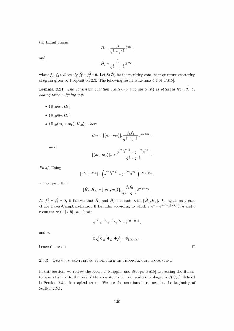
the Hamiltonians
H1 =f1
q12 − q−
12
zm1 ,
and
H2 =f2
q12 − q−
12
zm2 ,
where f1, f2 ∈ R satisfy f21 = f2
2 = 0. Let S(D) be the resulting consistent quantum scattering
diagram given by Proposition 2.3. The following result is Lemma 4.3 of [FS15].
Lemma 2.21. The consistent quantum scattering diagram S(D) is obtained from D by
adding three outgoing rays:
• (R⩾0m1, H1)
• (R⩾0m2, H2)
• (R⩾0(m1 +m2), H12), where
H12 ∶= [⟨m1,m2⟩]qf1f2
q12 − q−
12
zm1+m2 ,
and
[⟨m1,m2⟩]q ∶=q
⟨m1,m2⟩
2 − q−⟨m1,m2⟩
2
q12 − q−
12
.
Proof. Using
[zm1 , zm2] = (q⟨m1,m2⟩
2 − q−⟨m1,m2⟩
2 ) zm1+m2 ,
we compute that
[H1, H2] = [⟨m1,m2⟩]qf1f2
q12 − q−
12
zm1+m2 .
As f21 = f2
2 = 0, it follows that H1 and H2 commute with [H1, H2]. Using an easy case
of the Baker-Campbell-Hausdorff formula, according to which eaeb = ea+b+12 [a,b] if a and b
commute with [a, b], we obtain
eH2e−H1e−H2eH1 = e[H1,H2] ,
and so
Φ−1H2
ΦH1ΦH2
Φ−1H1
= Φ[H1,H2]
,
hence the result
2.6.3 Quantum scattering from refined tropical curve counting
In this Section, we review the result of Filippini and Stoppa [FS15] expressing the Hamil-
tonians attached to the rays of the consistent quantum scattering diagram S(Dm), defined
in Section 2.3.1, in tropical terms. We use the notations introduced at the beginning of
Section 2.5.1.
130

Proposition 2.22. For every m = (m1, . . . ,mn) an n-tuple of primitive non-zero vectors in
M and for every m ∈ M − 0, the Hamiltonian Hm attached to the outgoing ray R⩾0m in
the consistent quantum scattering diagram S(Dm) is given by
Hm = ∑p∈Pm
∑k⊢p
N tropw(k)
(q12 )
⎛
⎝
n
∏j=1
∏`⩾1
1
k`j !((−1)`−1
`
q12 − q−
12
q`2 − q−
`2
)
k`j⎞
⎠
⎛
⎝
n
∏j=1
tpjj
⎞
⎠
z`pm
q12 − q−
12
,
where q = eih, and the first sum is over all partitions k of p.
Proof. This follows from the main result, Corollary 4.9, of [FS15], which is a q-deformed
version of the proof of Theorem 2.8 of [GPS10]. A higher dimensional generalization of this
argument has been given by Mandel in [Man15]. For completeness and because we organize
the combinatorics in a slightly different way, we provide a proof.
By definition, S(Dm) is the consistent quantum scattering diagram obtained from the quan-
tum scattering diagram Dm consisting of incoming rays (di, Hdj), j = 1, . . . , n, where
dj = −R⩾0mj ,
and
Hdj =∑`⩾1
1
`
(−1)`−1
q`2 − q−
`2
t`j z`mj .
Let us work over the ring C[t1, . . . , tn]/(tN+11 , . . . , tN+1
n ). We embed this ring into
C[uja∣1 ⩽ j ⩽ n,1 ⩽ a ⩽ N]/⟨u2ja∣1 ⩽ j ⩽ n,1 ⩽ a ⩽ N⟩
by
tj =N
∑a=1
uja
for all 1 ⩽ j ⩽ n. We then have
t`j = ∑A⊂1,...,N
∣A∣=`
`! ∏a∈A
uja ,
and so
Hdj =N
∑`=1
∑A⊂1,...,N
∣A∣=`
(1
`
(−1)`−1
q`2 − q−
`2
) `!(∏a∈A
uja) z`mj .
This suggests to consider the quantum scattering diagram Dsplitm consisting of incoming rays
(dj`A, Hdj`A), 1 ⩽ ` ⩽ N , A ⊂ 1, . . . ,N, ∣A∣ = `, where
dj`A = −R⩾0mj + cj`A ,
for cj`A ∈ R2 in general position, and
Hdj`A = (1
`
(−1)`−1
q`2 − q−
`2
) `!(∏a∈A
uja) z`mj .
131

If we had taken all cj`A = 0, then Dsplitm would have been equivalent to Dm. But for cj`A ∈ R2
in general position, Dsplitm is a perturbation of Dm: each ray (dj , H∂j) of Dm splits into
various rays (dj`A, Hdj`A) of Dsplitm .
The key simplifying fact is that the consistent scattering diagram S(Dsplitm ) can be obtained
from Dsplitm by a recursive procedure involving only elementary scatterings in the sense of
Lemma 2.21. When two rays of Dsplitm intersect, we are in the situation of Lemma 2.21
because u2ja = 0. The local consistency at this intersection is then guaranteed by emitting a
third ray according to Lemma 2.21. Further intersections of the old and newly created rays
can similarly be treated by application of Lemma 2.21. Indeed, the assumptions of general
position of the cj`A guarantees that only double intersections occur.
The asymptotic scattering diagram of S(Dsplitm ) is the scattering diagram obtained by taking
all the rays of S(D) and placing their origin at 0 ∈ R2. By uniqueness of the consistent
completion, the asymptotic scattering diagram is precisely S(Dm). To get the Hamiltonian
Hm attached to an outgoing ray R⩾0m in S(Dm), it is then enough to collect the various
contributions to the corresponding asymptotic ray of S(Dsplitm ) coming from the recursive
construction of S(Dsplitm ).
Let us study how the recursive construction of S(Dsplitm ) can produce a ray d asymptotic to
R⩾0m and equipped with a function Hd proportional to z`dm, for some `d ⩾ 1. Such a ray
is obtained by successive applications of Lemma 2.21 starting from a subset of the initial
incoming rays of Dsplitm .
We focus on one particular sequence of such elementary scatterings. Such sequence naturally
defines a graph Γ in R2. This graph starts with unbounded edges given by the initial rays
taking part to the sequence of scatterings. When two of these rays meet, they scatter and
produce a third ray given by Lemma 2.21. If this third ray does not contribute to further
scatterings ultimately contributing to Hd, we do not include it in Γ and we continue Γ by
propagating the two initial rays. In particular, Γ contains a 4-valent vertex given by the two
initial rays crossing without non-trivial interaction.
If the third ray does contribute to further scatterings ultimately contributing to Hd, we
include it in Γ and we do not propagate the two initial rays. In particular, Γ gets a trivalent
vertex given by the two initial rays meeting and producing the third ray. Iterating this
construction, we get one trivalent vertex for each elementary scattering ultimately giving a
contribution to Hd. At the end of this process, the last elementary scattering produces the
ray d which becomes an unbounded edge of the graph.
The graph Γ has two kinds of vertices: trivalent vertices where a non-trivial elementary
scattering happens and 4-valent vertices where two rays cross without non-trivial interaction.
For every 4-valent vertices, we can separate the two rays crossing, and we get a trivalent
graph Γ and a map h∶Γ → Γ ⊂ R2 which is one to one except over the 4-valent vertices of Γ
where it is two to one. It follows from the iterative construction that the trivalent graph Γ
is a tree, i.e. a graph of genus zero.
The function attached to initial ray of Dsplitm is a monomial in z, whose power is proportional
to the direction of the ray. By Lemma 2.21, this property is preserved under elementary
132

scattering. Each edge E of our Γ is thus equipped with a function proportional to zmE
for some mE ∈ M = Z2 proportional to the direction of E. Furthermore, in an elementary
scattering of two edges E1 and E2 equipped with mE1 and mE2 , the produced edge E3
is equipped with mE1 +mE2 by Lemma 2.21. In other words, the balancing condition is
satisfied at each vertex and so we can view h∶Γ→ R2 as a parametrized tropical curve to R2
in the sense of Section 2.6.1.
For every 1 ⩽ j ⩽ n and ` ⩾ 1, there is a number k`j of subsets A of 1, . . . , n, of size `,
such that dj`A is one of the initial ray appearing in Γ. Denote by AΓj` this set of subsets of
1, . . . , n. Writing pj ∶= ∑`≥1 `k`j , we have by the balancing condition
n
∑j=1
pj = `dm,
and in particular `d = `p.
It follows from an iterative application of Lemma 2.21 that the contribution of Γ to Hd is
given by
mΓ(q12 )
⎛⎜⎝
n
∏j=1
∏`⩾1
((−1)`−1
`
q12 − q−
12
q`2 − q−
`2
)
k`j
(`!)k`j⎛⎜⎝∏
A∈AΓj`
∏a∈A
uja⎞⎟⎠
⎞⎟⎠
z`pm
q12 − q−
12
,
where mΓ(q12 ) is the refined multiplicity of the tropical curve Γ.
To get the complete expression for Hd, we have to sum over the possible Γ.
If we fix p = (p1, . . . , pn) ∈ P = Nn, k a partition of p and for every 1 ⩽ j ⩽ n and ` ⩾ 1, a set
Aj` of k`j disjoint subsets of 1, . . . ,N of size `, we can consider the set Tj`Aj` of genus zero
tropical curves Γ having one unbounded edge of asymptotic direction R⩾0m and weight `pm,
and for every 1 ⩽ j ⩽ n, ` ⩾ 1, A ∈ Aj`, an unbounded edge of weight `mj asymptotically
coinciding with dj`A. By Section 2.6.1, this set is finite.
We already saw how a sequence of elementary scatterings contributing to Hd produces
an element Γ ∈ Tj`Aj` . Conversely, any Γ ∈ Tj`Aj` will define a sequence of elementary
scatterings appearing in the construction of S(Dsplitm ) and contributing to Hd.
It follows that, for every m ∈M − 0, we have
Hm =
∑p∈Pm
∑k⊢p
∑Aj`
⎛⎜⎝
∑Γ∈Tj`Aj`
mΓ(q12 )
⎞⎟⎠
⎛
⎝
n
∏j=1
∏`⩾1
((−1)`−1
`
q12 − q−
12
q`2 − q−
`2
)
k`j
(`!)k`j⎛
⎝∏
A∈Aj`
∏a∈A
uja⎞
⎠
⎞
⎠
z`pm
q12 − q−
12
,
But by Section 2.6.1, we have
∑Γ∈Tj`Aj`
mΓ(q12 ) = N trop
w(k)(q
12 ) ,
which is in particular independent of Aj`. So we can do the sum over Aj`. Given an Aj`,
133

we can form
B ∶= ⋃A∈Aj`
A,
a subset of 1, . . . ,N of size ∑`⩾1 `k`j = pj . Conversely, the number of ways to write a set
B of pj = ∑`⩾1 `k`j elements as a disjoint union of subsets, k`j of them being of size `, is
equal topj !
∏`⩾1 k`j !(`!)k`j
.
Replacing the sum over Aj` by a sum over B, we get
Hm =
∑p∈Pm
∑k⊢p
N tropw(k)
(q12 )
⎛
⎝
n
∏j=1
∏`⩾1
1
k`j !((−1)`−1
`
q12 − q−
12
q`2 − q−
`2
)
k`j⎞
⎠
⎛⎜⎜⎜⎝
n
∏j=1
∑B⊂1,...,N
∣B∣=pj
pj !∏b∈B
ujb
⎞⎟⎟⎟⎠
z`pm
q12 − q−
12
,
Finally, using that
tpjj = ∑
B⊂1,...,N
∣B∣=pj
pj !∏b∈B
ujb ,
we obtain the desired formula for Hm.
Corollary 2.23. We have
Hm = ∑p∈Pm
∑k⊢p
N tropw(k)
(q12 )
⎛
⎝
n
∏j=1
∏`⩾1
1
k`j !((−1)`−1
`
1
q`2 − q−
`2
)
k`j⎞
⎠(q
12 − q−
12 )s(k)−1z`pm .
Proof. We simply rearrange (q12 − q−
12 ) factors in Proposition 2.22 and use that
s(k) =n
∑j=1
∑`⩾1
k`j .
2.7 End of the proof of Theorems 2.6 and 2.7
2.7.1 End of the proof of Theorem 2.6
In this Section, we finish the proof of Theorem 2.6. We have to express the Hamiltonians
attached to the rays of the consistent quantum scattering diagram S(Dm) in terms of the
log Gromov-Witten invariants NYmg,p of the log Calabi-Yau surface Ym.
We know already:
• Corollary 2.23, expressing the Hamiltonians attached to the rays of S(Dm) in terms
of the refined counts N tropw (q
12 ) of tropical curves in R2.
134

• Proposition 2.8, relating the log Gromov-Witten invariants NYmg,p of the log Calabi-Yau
surface Ym to the log Gromov-Witten invariants NY mg,w of the toric surface Y m.
It remains to connect the refined tropical counts N tropw (q
12 ) to the log Gromov-Witten in-
variants NY mg,w of the toric surface Y m. This is given by the following Proposition 2.24, which
is a special case of the main result, Theorem 1.4, of Chapter 1.
Proposition 2.24. For every m = (m1, . . . ,mn) n-tuple of non-zero primitive vectors in
M = Z2, every p = (p1, . . . , pn) ∈ P = Nn, and every k partition of p, we have
∑g⩾0
NY m
g,w(k)h2g−1+s(k)
= N tropw(k)
(q12 )
⎛
⎝
s(k)
∏r=1
1
∣wr ∣
⎞
⎠(2 sin(
h
2))
s(k)−1
= N tropw(k)
(q12 )
⎛
⎝
n
∏j=1
∏`⩾1
1
`k`j
⎞
⎠(2 sin(
h
2))
s(k)−1
.
Proof. We simply explain the change in notations needed to translate from Theorem 1.4.
In Chapter 1, we fixed a ∆ a balanced collection of vectors in Z2, specifying a toric surface
X∆ and tangency conditions for a curve along the toric divisors. We fixed a subset ∆F of
∆, for which the corresponding tangency conditions happen at prescribed positions on the
toric divisors. Finally, we fixed a non-negative integer n. Theorem 1.4 is a correspondence
theorem between log Gromov-Witten invariants of X∆, counting curves in X∆ satisfying
the tangency constraints imposed by ∆ and ∆F , and passing through n points in general
position, and refined counts of tropical curves in R2 satisfying the tropical analogue of these
constraints.
To get Proposition 2.24, we take ∆ = (w1(k), . . . ,ws(k)(k), kwmw)12, ∆F = (w1(k), . . . ,ws(k)(k))
and n = 0. Using the notations of Chapter 1, we have ∣∆∣ = s(k)+1, ∣∆F ∣ = s(k) and g∆F
∆,n = 0.
Using finally that the variable u keeping track of the genus in Chapter 1 is denoted h in the
present Chapter, we see that Theorem 1.4 reduces to Proposition 2.24.
By comparison of the explicit formulas of Corollary 2.23, Proposition 2.24 and Proposition 2.8,
and using the relation
s(k) =n
∑j=1
∑`⩾1
k`j
to collect the powers of i, we find exactly the formula given in Theorem 2.6 for the Hamiltoni-
ans of the quantum scattering diagram S(Dm) in terms of the log Gromov-Witten invariants
NYmg,p of the log Calabi-Yau surface Ym. This ends the proof of Theorem 2.6.
2.7.2 End of the proof of Theorem 2.7
The proof of Theorem 2.7 follows the one of Theorem 2.6, up to minor notational changes.
The only needed serious modification is an orbifold version of the multicovering formula of
Lemma 2.20. This is provided by Lemma 2.25 below.
12We then have X∆ = Y m up to some toric blow ups, which do not change the relevant log Gromov-Witteninvariants by [AW13].
135

We fix positive integers r and `. Let P1[r,1] be the stacky projective line with a single
orbifold point of isotropy group Z/r at 0. Let Mg,`(P1[r,1]/∞) be the moduli space of
genus g orbifold stable maps to P1[r,1], relative to ∞ ∈ P1[r,∞], of degree r`, with maximal
tangency order r` along ∞. It is a proper Deligne-Mumford stack of virtual dimension
2g − 1 + `, admitting a virtual fundamental class
[Mg,`(P1[r,1]/∞)]
virt∈ A2g−1+`(Mg,`(P1
[r,1]/∞),Q) .
Let OP1[r,1](−[0]/(Z/r)) be the orbifold line bundle on P1[r,1] of degree −1/r. Denoting
π∶C → Mg,`(P1[r,1]/∞) the universal source curve and f ∶C → P1[r,1] the universal map,
we define
N `g,r ∶= ∫
[Mg,`(P1[r,1]/∞)]virt(−1)gλg e (R
1π∗f∗ (OP1[r,1](−[0]/(Z/r)))) ∈ Q ,
where e(−) is the Euler class.
Lemma 2.25. For every positive integers r and `, we have
∑g⩾0
N `g,rh
2g−1=
(−1)`−1
`
1
2 sin ( r`h2
).
Proof. It is an higher genus version of Proposition 5.7 of [GPS10] and an orbifold version
of Theorem 5.1 of [BP05]. Very similar localization computations of higher genus orbifold
Gromov-Witten invariants can be found in [JPT11]. The main thing we need to explain is
the replacement in the orbifold case for the Mumford relation c(E)c(E∨) = 1 playing a key
role in the proof of Theorem 5.1 of [BP05]. We will simply have to twist the usual Hodge
theoretic argument of [Mum83] by a local system.
We consider the action of C∗ on P1[r,1] with tangent weights [1/r,−1] at the fixed points
[0,∞]. We choose the equivariant lifts of
OP1[r,1](−[0]/(Z/r))
and OP1[r,1] having fibers over the fixed points [0,∞] of weight [−1/r,0] and [0,0] respec-
tively. For such choices, the argument given in the proof of Theorem 5.1 of [BP05] shows
that only one graph Γ contributes to the C∗-localization formula computing N `g,r. The graph
Γ consists of a genus g vertex over 0, a unique edge of degree r` and a degenerate genus zero
vertex over ∞.
The contribution of Γ is computed using the virtual localization formula of [GP99]. The
corresponding C∗-fixed locus is13 the fiber product
Mg,1(BZ/r) ×IBZ/r BZ/(rd) ,
where Mg,1(BZ/r) is the moduli stack of 1-pointed14 genus g orbifold stable maps to the
classifying stack BZ/r, IBZ/r is the rigidified inertia stack of BZ/r, and the classifying
13We are assuming g > 0. The case g = 0 is simpler and treated in Proposition 5.7 of [GPS10].14With a trivial stacky structure at the marked point.
136

stack BZ/(rd) appears as moduli space of C∗-invariant Galois covers P1 → P1[r,1] of degree
r`. This fibered product is a cover of Mg,1(BZ/r) of degree r/(r`).
We denote π0∶C0 →Mg,1(BZ/r) the universal source curve over Mg,1(BZ/r). The data of
an orbifold stable map f0∶C0 → BZ/r is equivalent to the data of an (orbifold) Z/r-local
system L on C0. We denote by t the generator of the C∗-equivariant cohomology of a point.
The computation of the inverse of the equivariant Euler class of the equivariant virtual
bundle is done in Section 2.2 [JPT11] and gives
e(R1(π0)∗ (OC0 ⊗L⊗
t
r))
(r`)`
t``!
1tr`− ψ
(r
t)δL,0 t
r,
where δL,0 = 1 if L is the trivial Z/r-local system and 0 else. The vector bundle
R1(π0)∗ (OC0 ⊗L⊗
t
r)
over Mg,1(BZ/r) comes from the equivariant orbifold line bundle TP1[r,1](−∞)∣[0]/(Z/r) over
BZ/r, restriction over [0]/(Z/r) of the degree 1/r orbifold line bundle TP1[r,1](−∞) over
P1[r,1].
The contribution of the integrand in the definition of N `g,r is
(−1)gλge(R1(π0)∗ (OC0 ⊗ (L⊗
t
r)∨
))(−t
r)
1−δR,0
(−1)`−1 (` − 1)!
(r`)`−1t`−1 .
The vector bundle R1(π0)∗ (OC0 ⊗ (L⊗ tr)∨) over Mg,1(BZ/r) comes from the equivariant
orbifold line bundle OP1[r,1](−[0]/(Z/r))∣[0]/(Z/r) over BZ/r, restriction over [0]/(Z/r) of
the degree −1/r orbifold line bundle OP1[r,1](−[0]/(Z/r)) over P1[r,1].
By Serre duality, we have
R1(π0)∗ (OC0 ⊗ (L⊗
t
r)∨
) = ((π0)∗ (ωπ0 ⊗L⊗t
r))
∨
,
and so
e(R1(π0)∗ (OC0 ⊗ (L⊗
t
r)∨
)) = (−1)rke((π0)∗ (ωπ0 ⊗L⊗t
r))
= (−1)rk(t
r)
rk rk
∑j=0
(r
t)j
cj ((π0)∗ (ωπ0 ⊗L))
= (−1)rk(t
r)
rk
c rt((π0)∗(ωπ0 ⊗L)) ,
where rk is the rank of (π0)∗ (ωπ0 ⊗L), locally constant function on Mg,1(BZ/r), equal to
g on the component with L trivial and to g − 1 on the components with L non-trivial, and
where
cx(E) ∶=∑j⩾0
xjcj(E)
137
is the Chern polynomial of a vector bundle E. Similarly, we have
e(R1(π0)∗ (OC0 ⊗L⊗
t
r)) = (
t
r)
rk rk
∑j=0
(r
t)j
cj (R1(π0)∗ (OC0 ⊗L))
= (t
r)
rk
c rt(R1
(π0)∗ (OC0 ⊗L)) .
We twist now the Hodge theoretic argument of [Mum83] (see formulas (5.4) and (5.5)) (see
also Proposition 3.2 of [BGP08]) by the local system L. The complex
ωC0∶0→ OC0
dÐ→ ωπ0 → 0 ,
twisted by L, gives rise to an exact sequence
0→ (π0)∗(ωπ0 ⊗L)→ R1(π0)∗(ω
C0⊗L)→ R1
(π0)∗(OC0 ⊗L)→ 0 .
By Hodge theory, we have the Gauss-Manin connection on the restriction of R1(π0)∗(ωC0⊗L)
to the open dense subset of Mg,1(BZ/r) given by smooth curves, with regular singularities
and nilpotent residue along the divisor of nodal curves. This is enough to imply
cx (R1(π0)∗(ω
C0⊗L)) = 1 ,
and so
cx ((π0)∗(ωπ0 ⊗L)) cx (R1(π0)∗(OC0 ⊗L)) = 1 .
Using this relation to simplify the above expressions, we get
N `g,r =
r
r`∫Mg,1(BZ/r)
(−1)`−1(−1)g+rk+1−δL,0 (
t
r)
2 rk−2δL,0+1 λgtr`− ψ
.
Using that rk = g − 1 + δR,0, this can be rewritten as
N `g,r = ∫
Mg,1(BZ/r)
(−1)`−1
`(t
r)
2g−1 λgtr`− ψ
.
As the dimension of Mg,1(BZ/r) is 3g−2, we have to extract the term proportional to ψ2g−2
and we get
N `g,r = ∫
Mg,1(BZ/r)
(−1)`−1
``2g−1λgψ
2g−2 .
The integrand is now pullback from the moduli space Mg,1 of 1-pointed genus g stable maps.
As the forgetful map Mg,1(BZ/r)→Mg,n has degree15 r2g−1, we have
N `g,r =
(−1)`−1
`(r`)2g−1
∫Mg,1
λgψ2g−2 ,
and the result then follows, as in the proof of Theorem 5.1 of [BP05], from the Hodge
integrals computations of [FP00].
15There are r2g Z/r-local systems on a smooth genus g curve, each with a Z/r group of automorphisms.
138

2.8 Integrality results and conjectures
In Section 2.8.1, we state Conjecture 2.28, a log BPS integrality conjecture. In Section 2.8.2,
we state Theorem 2.30, precise version of Theorem 3 of the Introduction, establishing the
validity of Conjecture 2.28 for (Ym, ∂Ym). The proof of Theorem 3 takes Sections 2.8.3
and 2.8.4. In Section 2.8.5, we describe some explicit connection with refined Donaldson-
Thomas theory of quivers. Finally, in Section 2.8.6, we discuss del Pezzo surfaces with a
smooth anticanonical divisor and we formulate Conjecture 2.41, precise form of Conjecture 4
of the Introduction.
2.8.1 Integrality conjecture
We formulate a higher genus analogue of the log BPS integrality conjecture, Conjecture 6.2,
of [GPS10]. We start by formulating a rationality conjecture, Conjecture 2.26, before stating
the integrality conjecture, Conjecture 2.28.
Let Y be a smooth projective surface and let ∂Y ⊂ Y be a reduced normal crossing effective
divisor. We endow Y with the divisorial log structure defined by ∂Y and we get a smooth
log scheme. Following Section 6.1 of [GPS10], we say that (Y, ∂Y ) is log Calabi-Yau with
respect to some non-zero class β ∈H2(Y,Z) if β.(∂Y ) = β.(−KY ).
Two basic examples are:
• For every m = (m1, . . . ,mn) an n-tuple of primitive non-zero vectors in M = Z2, the
pair (Ym, ∂Ym)16 defined in Section 2.2.1. Then (Ym, ∂Ym) is log Calabi-Yau with
respect to every class β ∈ H2(Ym,Z) and so in particular with respect to the classes
βp ∈H2(Ym,Z) defined in Section 2.2.2.
• Y a del Pezzo surface and ∂Y a smooth anticanonical divisor. Then (Y, ∂Y ) is log
Calabi-Yau with respect to every class β ∈H2(Y,Z).
We fix (Y, ∂Y ) log Calabi-Yau with respect to some β ∈ H2(Y,Z) such that β.(∂Y ) ≠ 0.
Let Mg,β(Y /∂Y ) be the moduli space of genus g stable log maps to Y of class β and full
tangency of order β.(∂Y ) at a single unspecified point of D. It is a proper Deligne-Mumford
stack of virtual dimension g admitting a virtual fundamental class
[Mg,β(Y /∂Y )]virt
∈ Ag(Mg,β(Y /∂Y ),Q) .
We define
NY /∂Yg,β ∶= ∫
[Mg,β(Y /∂Y )]virt(−1)gλg ∈ Q .
Remark that if (Y, ∂Y ) is of the form (Ym, ∂Ym) and β is of the form βp, see Section 2.2.2,
then we have NY /∂Yg,β = NYm
g,p where NYmg,p are the invariants defined in Section 2.2.3.
We can now formulate the rationality conjecture.
16Strictly speaking, Ym is not smooth, but log smooth. We can either make Ym smooth by toric blow-upsor allow log smooth objects in the definition of log Calabi-Yau.
139

Conjecture 2.26. Let (Y, ∂Y ) be a log Calabi-Yau pair with respect to some class β ∈
H2(Y,Z) such that β.(∂Y ) ≠ 0. Then there exists a rational function
Ωβ(q12 ) ∈ Q(q±
12 )
such that we have the equality of power series in h,
Ωβ(q12 ) = (−1)β.(∂Y )+1
(2 sin(h
2))
⎛
⎝∑g⩾0
NY /∂Yg,β h2g−1⎞
⎠,
after the change of variables q = eih.
Remarks:
• Ωβ(q12 ) is unique if it exists.
• If the rational function Ωβ(q12 ) exists, then it is invariant under q
12 ↦ q−
12 , because its
power series expansion in h after q = eih has real coefficients.
• Given the 3-dimensional interpretation of the invariants NY,∂Yg,β given in Section 2.2.4,
Conjecture 2.26 should follow from a log version of the MNOP conjectures, [MNOP06a],
[MNOP06b], once an appropriate theory of log Donaldson-Thomas invariants is devel-
oped. If ∂Y is smooth, then Conjecture 2.26 indeed follows from the relative MNOP
conjectures, see Section 3.3 of [MNOP06b].
Let (Y, ∂Y ) be a log Calabi-Yau pair with respect to some primitive class β ∈H2(Y,Z) such
that β.(∂Y ) ≠ 0. Let us assume that Conjecture 2.26 is true for all the classes multiple of β.
So, for every n ⩾ 1, we have a rational function Ωnβ(q12 ) ∈ Q(q±
12 ). We define a collection of
rational functions Ωnβ(q12 ) ∈ Q(q±
12 ), n ⩾ 1, invariant under q
12 ↦ q−
12 , by the relations
Ωnβ(q12 ) =∑
`∣n
1
`
q12 − q−
12
q`2 − q−
`2
Ωn` β
(q`2 ) .
Lemma 2.27. These relations have a unique solution, given by
Ωnβ(q12 ) =∑
`∣n
µ(`)
`
q12 − q−
12
q`2 − q−
`2
Ωn` β
(q`2 ) ,
where µ is the Mobius function.
Proof. Indeed, we have
∑`∣n
1
`
q12 − q−
12
q`2 − q−
`2
⎛
⎝∑`′∣n`
µ(`′)
`′q`2 − q−
`2
q``′
2 − q−``′
2
Ω n``′β(q
``′
2 )⎞
⎠
=∑`∣n
∑`′∣n`
µ(`′)
``′q
12 − q−
12
q``′
2 − q−``′
2
Ω n``′β(q
``′
2 ) = ∑m∣n
1
m
q12 − q−
12
qm2 − q−
m2
Ω nmβ
(qm2 )
⎛
⎝∑`′∣m
µ(`′)⎞
⎠
140

= ∑m∣n
1
m
q12 − q−
12
qm2 − q−
m2
Ω nmβ
(qm2 )δm,1 = Ωnβ(q
12 ) ,
where we used the Mobius inversion formula ∑`′∣m µ(`′) = δm,1.
We can now formulate the integrality conjecture.
Conjecture 2.28. Let (Y, ∂Y ) be a log Calabi-Yau pair with respect to some class β ∈
H2(Y,Z), such that β.(∂Y ) ≠ 0, and such that the rationality Conjecture 2.26 is true for all
multiples of β, so that the rational functions Ωnβ(q12 ) ∈ Q(q±
12 ), are defined. Then, in fact,
for every n ⩾ 1, Ωnβ(q12 ) is a Laurent polynomial in q
12 with integer coefficients, i.e.
Ωnβ(q12 ) ∈ Z[q±
12 ] ,
invariant under q12 ↦ q−
12 .
Remark:
• In Section 2.9.3, we explain why this integrality conjecture can be interpreted in some
cases as a mathematically well-defined example of the general integrality for open
Gromov-Witten invariants in Calabi-Yau 3-folds predicted by Ooguri-Vafa [OV00]. In
particular, the log BPS invariants Ωβ(q12 ) should be thought as examples of Ooguri-
Vafa/open BPS invariants.
• In the classical limit h → 0, the integrality of Ωnβ ∶= Ωnβ(q12 = 1) is equivalent to
Conjecture 6.2 of [GPS10].
• If β2 = −1, β.(∂Y ) = 1, and the class β only contains a smooth rational curve, then
it follows from Lemma 2.20 that Conjecture 2.28 is true. More precisely, we have
Ωnβ(q12 ) = 1
nq
12 −q−
12
qn2 −q−
n2
for every n ⩾ 1, and so Ωβ(q12 ) = 1 and Ωnβ(q
12 ) = 0 for n > 1.
2.8.2 Integrality result
Lemma 2.29. For every m = (m1, . . . ,mn) an n-tuple of primitive non-zero vectors in
M = Z2 and p ∈ P = Nn, the rationality Conjecture 2.26 is true for the log Calabi-Yau pair
(Ym, ∂Ym) with respect to the curve class βp ∈H2(Y,Z).
Proof. This follows from Theorem 2.6, expressing the generating series of invariants NYmg,p
as a Hamiltonian Hm attached to some ray of the quantum scattering diagram S(Dm),
and from Proposition 2.22, giving a formula for Hm whose coefficients are manifestly in
Q[q±12 ][(1 − q`)−1]`⩾1.
Alternatively, one could argue that, because the initial quantum scattering diagram Dm
is defined over Q[q±12 ][(1 − q`)−1]`⩾1, the resulting consistent quantum scattering diagram
S(Dm) is also defined over Q[q±12 ][(1 − q`)−1]`⩾1 and so Lemma 2.29 follows directly from
Theorem 2.6.
141

By Lemma 2.29, we have rational functions
ΩYm
p (q12 ) ∈ Q(q±
12 ) ,
such that
ΩYm
p (q12 ) = (−1)`p+1
(2 sin(h
2))
⎛
⎝∑g⩾0
NYmg,p h
2g−1⎞
⎠,
as power series in h, after the change of variables q = eih. Remark that we used the fact
that βp.(∂Ym) = `p.
The following result is, after Theorem 2.6, the second main result of this Chapter. It is the
precise form of Theorem 3 in the Introduction.
Theorem 2.30. For every m = (m1, . . . ,mn) an n-tuple of primitive non-zero vectors in
M = Z2 and p ∈ P = Nn, the integrality Conjecture 2.28 is true for the log Calabi-Yau pair
(Ym, ∂Ym) with respect to the class βp ∈ H2(Ym,Z). In other words, there exists ΩYmp (q
12 ) ∈
Z[q±12 ] such that
ΩYm
p (q12 ) = ∑
p=`p′
1
`
q12 − q−
12
q`2 − q−
`2
ΩYm
p′ (q`2 ) .
The proof of Theorem 2.30 takes the next Sections 2.8.3 and 2.8.4.
2.8.3 Quadratic refinement
According to Theorem 2.6, generating series of the log Gromov-Witten invariants NYmg,p
are Hamiltonians attached to the rays of some quantum scattering diagram S(Dm). Our
integrality result, Theorem 2.30, will follow from a general integrality result for scattering
diagrams. Our main input, the integrality result of [KS11], is phrased in terms of twisted
quantum scattering diagrams, i.e. scattering diagrams valued in automorphisms of twisted
quantum tori. The comparison with quiver DT invariants, done in Section 2.8.5, also requires
to consider twisted quantum scattering diagrams.
In the present Section, we explain how to compare the quantum scattering diagram S(Dm)
with a twisted quantum scattering diagram S(Dtwm ). This comparison requires the notion
of quadratic refinement. A short and to the point discussion by Neitzke can be found in
[Nei14]. Some related discussion can be found in Appendix A of [Lin17].
We start with P = Nn = ⊕nj=1Nej . For p = (p1, . . . , pn) ∈ P = Nn, we denote ord(p) ∶= ∑nj=1 pj .
An n-tuple m = (m1, . . . ,mn) of primitive non-zero vectors in M = Z2 naturally defines an
additive map
r∶P →M
ej ↦mj .
For every A a Z[q±12 ]-algebra, we denote TAP,tw the non-commutative “space” whose algebra
of functions is the algebra Γ(OTAP,tw
) given by A[[P ]], powers series in xp, p ∈ P , with
142

coefficients in A, with the product defined by
xp.xp′
= (−1)⟨r(p),r(p′)⟩q
12 ⟨r(p),r(p
′)⟩xp+p
′
.
The main difference with respect to the formalism of Section 2.1 is the twist by the extra
sign (−1)⟨r(p),r(p′)⟩.
We will use A = Z[[q±12 ]], Z((q
12 )) and Q((q
12 )). We have obviously the inclusions
Γ(OT
Z[[q±1/2]]
P,tw
) ⊂ Γ(OT
Z((q1/2))
P,tw
) ⊂ Γ(OT
Q((q1/2))
P,tw
) .
Every
Htw= ∑p∈P
Htwp xp ∈ Γ(O
TQ((q1/2))
P,tw
) ,
such that Htw = 0 mod P , defines via conjugation by exp (Htw) an automorphism
ΦtwHtw = Adexp(Htw)
= exp (Htw) (−) exp (−Htw)
of Γ(OT
Q((q1/2))
P,tw
).
Definition 2.31. A twisted quantum scattering diagram Dtw over (r∶P →M) is a set of
rays d in MR, equipped with elements
Htwd ∈ Γ(O
TQ((q1/2))
P,tw
) ,
such that:
• There exists (a necessarily unique) p ∈ P primitive such that Htwd ∈ xpQ((q
12 ))[[xp]]
and either r(p) ∈ −N⩾1md or r(p) ∈ N⩾1md. We say that the ray (d, Htwd ) is ingoing
if r(p) ∈ −N⩾1md and outgoing if r(p) ∈ N⩾1md. We call p the P -direction of the ray
(d, Htwd ).
• For every ` ⩾ 0, there are only finitely many rays d of P -direction p satisfying ord(p) ⩽
`.
Using the automorphisms ΦtwHtw
, we define as in Section 2.1.4 the notion of consistent twisted
quantum scattering diagram and one can prove that every twisted quantum scattering dia-
gram Dtw can be canonically completed by adding only outgoing rays to form a consistent
twisted quantum scattering diagram S(Dtw).
The following Lemma will give us a way to go back and forth between quantum scattering
diagrams and twisted quantum scattering diagrams.
Lemma 2.32. The map σM ∶M → ±1, defined by σM(0) = 1 and σM(m) = (−1)∣m∣ for
m ∈M non-zero, where ∣m∣ is the divisibility of m in M , is a quadratic refinement of
∧2M → ±1
143

(m1,m2)↦ (−1)⟨m1,m2⟩ ,
i.e. we have
σM(m1 +m2) = (−1)⟨m1,m2⟩σM(m1)σM(m2) ,
for every m1,m2 ∈M . It is the unique quadratic refinement such that σM(m) = −1 for every
m ∈M primitive.
Proof. We fix a basis of M and we denote m = (mx,my) the coordinates of some m ∈M in
this basis. We define σ′M ∶M → ±1 by
σ′M(m) = (−1)mxmy+mx+my .
It is easy to check that σ′M is a quadratic refinement of (−1)⟨−,−⟩: the parity of
(mx1 +m
x2)(m
y1 +m
y2) +m
x1 +m
x2 +m
y1 +m
y2
differs from the parity of
mx1m
y1 +m
x1 +m
y1 +m
x2m
y2 +m
x2 +m
y2
by mx1m
y2 +m
x2m
y1, which has the parity of ⟨m1,m2⟩.
If m ∈M is primitive, then (mx,my) is equal to (1,0), (0,1) or (1,1) modulo two, and in
all these three cases, we get σ′M(m) = −1. Combined with the fact that σ′M is a quadratic
refinement, this implies that, for every m ∈M , we have σ′M(m) = (−1)∣m∣, i.e. σ′M = σM . In
particular, σM is a quadratic refinement and σ′M is independent of the choice of basis.
The uniqueness statement follows from the fact that a quadratic refinement is determined
by its value on a basis of M .
Let Dtwm be the twisted quantum scattering diagram consisting of incoming rays (dj , H
twdj ),
1 ⩽ j ⩽ n, where
dj = −R⩾0mj ,
and
Htwdj = −∑
`⩾1
1
`
1
q`2 − q−
`2
x`ej ∈ Γ(OT
Q((q1/2))
P,tw
) ,
where we consider1
q`2 − q−
`2
= −q`2 ∑k⩾0
qk` ∈ Q((q12 )) .
Let S(Dtwm ) be the corresponding consistent twisted quantum scattering diagram obtained
by adding only outgoing rays.
Define σP ∶P → ±1 by σP ∶= σM r. It follows from Lemma 2.32 that σP is a quadratic
refinement and so⎛
⎝
n
∏j=1
tpjj
⎞
⎠zr(p) ↦ σP (p)xp ,
is an algebra isomorphism between quantum tori and twisted quantum tori. Using this
144

isomorphism, we can construct a twisted quantum scattering diagram S(Dm)tw from the
quantum scattering diagram Dm.
The incoming rays of S(Dm)tw are (dj , Htwdj ), 1 ⩽ j ⩽ n, where dj = −R⩾0mj and
Htwdj = −∑
`⩾1
1
`
1
q`2 − q−
`2
x`ej .
The outgoing rays of S(Dm)tw are (R⩾0m,Htwm ) where
Htwm = − ∑
p∈Pm
Ωp(q12 )
q12 − q−
12
xp = − ∑p∈Pm
∑p=`p′
1
`
1
q`2 − q−
`2
ΩYm
p′ (q`2 )xp .
Lemma 2.33. We have S(Dtwm ) = S(Dm)tw.
Proof. As (∏nj=1 t
pjj )zr(p) ↦ σP (p)xp is an algebra isomorphism, the twisted quantum scat-
tering diagram S(Dm)tw is consistent and so the result follows from the uniqueness of the
consistent completion of twisted quantum scattering diagrams.
2.8.4 Proof of the integrality theorem
We give below the proof of Theorem 2.30. It is a combination of the scattering arguments
of Appendix C3 of [GHKK18] with the formalism of quantum admissible series of [KS11].
Because of the structure of the induction argument, we will in fact prove a more general
statement than Theorem 2.30. We will prove, Proposition 2.35, that the consistent comple-
tion of any (twisted) quantum scattering with incoming rays equipped with Hamiltonians
satisfying some BPS integrality condition has outgoing rays equipped Hamiltonians satisfy-
ing the BPS integrality condition.
We fix p ∈ P primitive. Consider
Htw=∑`⩾1
Htw` (q
12 )x`p ∈ xpQ((q
12 ))[[xp]] .
We define
Ω`(q12 ) ∶= −(q
12 − q−
12 )Htw
` (q12 ) ∈ Q((q
12 )) ,
and
Ω`(q12 ) ∶=∑
`′∣`
µ(`′)
`′q
12 − q−
12
q`2 − q−
`2
Ω ``′(q
`2 ) ∈ Q((q
12 )) .
It follows from Lemma 2.27 that we have
Htw= −∑
n⩾1∑`⩾1
1
`
Ωn(q`2 )
q`2 − q−
`2
x`np .
Definition 2.34. We say that Htw ∈ xpQ((q12 ))[[xp]] satisfies the BPS integrality condition
if the corresponding Ωl(q12 ) ∈ Q((q
12 )) are in fact Laurent polynomials with integer coeffi-
cients, i.e. Ω`(q12 ) ∈ Z[q
12 ].
145

Remarks:
• Htw satisfies the BPS integrality condition if and only if exp (Htw) is admissible in
the sense of Section 6 of [KS11].
• It follows from the product form of the quantum dilogarithm, as recalled in Section
2.3.1, that if Htw satisfies the BPS integrality condition, then ΦtwHtw
preserves the
subring Γ(OT
Z[[q1/2]]
P,tw
) of Γ(OT
Q((q1/2))
P,tw
). We call BPS quantum tropical vertex group17
the subgroup of automorphisms of Γ(OT
Z[[q1/2]]
P,tw
) generated by automorphisms of the
form ΦtwHtw
with Htw satisfying the BPS integrality condition.
We fix a choice of twisted quantum scattering diagram in each equivalence class by consider-
ing as distinct rays with different P -directions and by merging rays with coinciding supports
and with the same P -direction.
Proposition 2.35. Let nI be a positive integer and (p1, . . . , pnI ) be an nI-tuple of primitive
vectors in P . Let Dtw be a twisted quantum scattering diagram over (r∶P →M), consisting
of incoming rays (dj , Htwdj ), 1 ⩽ j ⩽ nI , with dj = −R⩾0r(p
j) and Htwdj ∈ xp
j
Q((q12 ))[[xp
j
]]
satisfying the BPS integrality condition. Then the consistent twisted quantum scattering
diagram S(Dtw) is such that for every outgoing ray (d, Htwd ), of P -direction p ∈ P , we have
that Htwd ∈ xpQ((q
12 ))[[xp]] satisfies the BPS integrality condition.
Proof. If nI = 2, or if more generally all the initial rays −Rr(pj) are contained in a common
half-plane of MR, then the result follows directly from Proposition 9 of [KS11].
We will reduce the general case to the case nI = 2 by using an argument parallel to the one
used in Appendix C.3 of [GHKK18] to prove some positivity property of classical scattering
diagrams.
For p = (p1, . . . , pn) ∈ P = Nn, we denote ord(p) ∶= ∑nj=1 pj . It is simply the total degree of
the monomial in several variables ∏nj=1 t
pjj .
The result we will prove by induction over some positive integer N is:
Proposition 2.36. Let n be a positive integer and r∶P = Nn → M be an additive map.
Let nI be a positive integer and (p1, . . . , pnI ) be an nI-tuple of primitive vectors in P .
Let Dtw be a twisted quantum scattering diagram over (r∶P → M), consisting of incoming
rays (dj , Htwdj ), 1 ⩽ j ⩽ nI , with dj = −R⩾0r(p
j) and Htwdj ∈ xp
j
Q((q12 ))[[xp
j
]] satisfying
the BPS integrality condition. Then every outgoing ray (d, Htwd ) of the consistent twisted
quantum scattering diagram S(Dtw), whose P -direction p satisfies ord(p) ⩽ N , is such that
Htwd ∈ xpQ((q
12 ))[[xp]] satisfies the BPS integrality condition.
Proposition 2.36 is obviously true for N = 1: the only outgoing rays with P -direction p
satisfying ord(p) = 1 are obtained by straight propagation of the initial rays and so satisfy
the BPS integrality condition if it is the case for the initial rays.
17Called the quantum tropical vertex group in [KS11] .
146

Let N > 1 be an integer. We assume by induction that Proposition 2.36 is true for all
integers strictly less than N and we want to prove it for N . As in Step III of Appendix C3
of [GHKK18], up to applying the perturbation trick, consisting in separating transversally
and generically the initial rays with the same support and then looking at the new local
scatterings, we can assume that at most two initial rays have order one.
We now use the change of monoid trick, as in Steps I and IV of Appendix C3 of [GHKK18].
Denote P ′ = ⊕nIj=1Ne
′j and
r′∶P ′→M
e′j ↦ r′(ej) ∶= r(pj) .
Let Dtw′
be the twisted quantum scattering diagram over (r′∶P ′ →M) obtained by replacing
xpj
by xe′
j in Htwdj . Denote
u∶P ′→ P
e′j ↦ pj .
Let (d, Htwd ) be an outgoing ray of S(Dtw), whose P -direction p satisfies ord(p) = N . Then
(d, Htwd ) is the sum of images by u of outgoing rays of S(Dtw′
), of P ′-direction mapping to
p by u. Let (d′, Htwd′ ) be such outgoing ray of S(Dtw′
).
Writing p′ = ∑nIj=1 p
′je′j , (p′1, . . . , p
′n) ∈ NnI , we have
ord(p′) = ord⎛
⎝
nI
∑j=1
p′je′j
⎞
⎠=nI
∑j=1
p′j ,
whereas
ord(p) = ord⎛
⎝
nI
∑j=1
p′jpj⎞
⎠=nI
∑j=1
p′j ord(pj) .
If only two p′j are non-zero, then the ray (d′, Htwd′ ) belongs to a twisted quantum scattering
diagram with two incoming rays and so its BPS integrality follows from Proposition 9 of
[KS11]. If more than two of the p′j are non-zero, then, at least one of the pj with nj ≠ 0
satisfies ord(pj) ⩾ 2 and so ord(p′) < ord(p). The BPS integrality of the ray (d′, Htwd′ ) then
follows by the induction hypothesis.
We can now finish the proof of Theorem 2.30. By Theorem 2.6 and Lemma 2.33, it is enough
to show that the outgoing rays of the twisted quantum scattering diagram S(Dtwm ) satisfy
the BPS integrality condition. As the initial rays of S(Dtwm ) satisfy the BPS integrality
condition, the result follows from Proposition 2.35.
2.8.5 Integrality and quiver DT invariants
We refer to [KS08], [JS12], [Rei10], [Rei11], [MR17] for Donaldson-Thomas (DT) theory of
quivers.
For every m = (m1, . . . ,mn) an n-tuple of primitive non-zero vectors in M = Z2, we define
147

a quiver Qm, with set of vertices 1,2, . . . , n and, for every 1 ⩽ j, k ⩽ n, ⟨mj ,mk⟩+ ∶=
max(⟨mj ,mk⟩,0) arrows from the vertex j to the vertex k. We identify P = ⊕nj=1Nej with
the set of dimension vectors for the quiver Qm.
Lemma 2.37. The quiver Qm is acyclic, i.e. does not contain any oriented cycle, if and
only if the n vectors m1, . . . ,mn are all contained in a closed half-plane of MR = R2.
Proof. The quiver Qm contains an arrow from the vertex i to the vertex j if and only if
(mi,mj) is an oriented basis of R2.
Let us assume that the quiver Qm is acyclic. Every θ = (θj)1⩽j⩽n ∈ Zn defines a notion
of stability for representations of Qm. For every p ∈ P , we then have a projective variety
Mθ−ssp , moduli space of θ-semistable representations of Qm of dimension p, containing the
open smooth locus Mθ−stp of θ-stable representations. Denote ι∶Mθ−st
p →Mθ−ssp the natural
inclusion. The main result of [MR17] is that the Laurent polynomials
ΩQm,θp (q
12 ) ∶= (−1)dimMθ−ss
p q−12 dimMθ−ss
p
dimMθ−stp
∑j=0
(dimH2j(Mθ−ss
p , ι!∗Q)) qj
∈ (−1)dimMθ−ssp q−
12 dimMθ−ss
p N[q]
are the refined DT invariants of Qm for the stability θ. In the above formula, ι!∗ is the
intermediate extension functor defined by ι and so ι!∗Q is a perverse sheaf on Mθ−ssp .
As Qm is acyclic, we can assume, up to relabeling m1, . . . ,mn, that ⟨mj ,mk⟩ ⩾ 0 if j ⩽ k.
If θ1 < θ2 < ⋅ ⋅ ⋅ < θn, then ΩQm,θej (q
12 ) = 1, for all 1 ⩽ j ⩽ n, and ΩQm,θ
p (q12 ) = 0 for p ∈
P − e1, . . . , en. We call such θ a trivial stability condition.
If θ1 > θ2 > ⋅ ⋅ ⋅ > θn, we call θ a maximally non-trivial stability condition. We simply denote
ΩQmp (q
12 ) for ΩQm,θ
p (q12 ) and θ a maximally non-trivial stability condition.
Theorem 2.38. For every m = (m1, . . . ,mn) such that the quiver Qm is acyclic, for every
p ∈ P = Nn, we have the equality
ΩQmp (q
12 ) = ΩYm
p (q12 )
between the refined DT invariant ΩQmp (q
12 ) of the quiver Qm and the log BPS invariant
ΩYmp (q
12 ) of the log Calabi-Yau surface Ym.
Proof. The twisted quantum scattering diagram S(Dtwm ) controls the wall-crossing of refined
DT invariants of Qm from the trivial stability condition to the maximally non-trivial stability
condition.
Remarks:
• In the limit q12 → 1, and if Qm is complete bipartite, then Theorem 2.38 reduces to
the Gromov-Witten/Kronecker correspondence of [GP10], [RW13], [RSW12].
148

• Theorem 2.38 can be viewed as a concrete example of equality between open BPS
invariants and DT invariants of quivers. The expectation for this kind of relation goes
back at least to [CV09], as reviewed in Section 2.9. Related recent stories include
[KRSS17a], [KRSS17b], where some knot invariants, which via some string theoretic
duality should be examples of open BPS invariants, are identified with some quiver DT
invariants, and [Zas18], where a precise correspondence between open BPS invariants
of some class of Lagrangian submanifolds in C3 and some DT invariants of quivers is
conjectured.
• Theorem 2.38 gives a different proof of Theorem 2.30 when Qm is acyclic. When Qm
is not acyclic, it is unclear a priori how to relate the log BPS invariants ΩYmp (q
12 ) to
some DT quiver theory. In the physics language, one should remove the contributions
of non-trivial single-centered (pure Higgs) indices (see [MPS13] and follow-ups). It
is still an open question to define mathematically the corresponding operation in DT
quiver theory. The fact that the integrality given by Theorem 2.30 holds even if Qm
is not acyclic is probably an additional evidence that it should be possible.
• When Qm is acyclic, Theorem 2.38 gives a positivity result for the log BPS invariants
ΩYmp (q
12 ). It is unclear how to prove a similar positivity result if Qm is not acyclic.
We finish this Section by some remark about signs. The definition of ΩYmp (q
12 ) given in
Section 2.8.2 includes a global sign (−1)`p−1 = (−1)βp.(∂Ym)−1, whereas the formula given
above for ΩQmp (q
12 ) includes a global sign (−1)dimMθ−ss
p . Using that βp.(∂Ym) and β2p have
the same parity by Riemann-Roch on Ym, the following result gives a direct proof that these
two signs are identical.
Lemma 2.39. For every p ∈ P , we have
dimMθ−ssp = β2
p + 1 .
Proof. We write p = ∑nj=1 pjej ∈ P . By standard quiver theory, we have
dimMθ−ssp =
n
∑j=1
n
∑k=1
⟨mj ,mk⟩+pjpk −n
∑j=1
p2j + 1 .
By definition, Section 2.2.2, we have
βp = ν∗β −
n
∑j=1
pjEj ,
where ν∶Ym → Y m is the blow-up morphism and β ∈H2(Y m,Z) is defined by some intersec-
tion numbers. It follows that
β2p = β
2−
n
∑j=1
p2j .
From the intersection numbers defining β, we see that the convex polygon dual to β is
obtained by successively adding the vectors pjmj and `pmp, in the order given by the
counterclockwise ordering of the mj and mp given by their argument. By standard toric
149

geometry, β2 is given by twice the area of the dual polygon and so we have
β2=
n
∑j=1
n
∑k=1
⟨mj ,mk⟩+pjpk .
It follows that
β2p =
n
∑j=1
n
∑k=1
⟨mj ,mk⟩+pjpk −n
∑j=1
p2j = dimMθ−ss
p − 1 .
2.8.6 del Pezzo surfaces
In this Section, we study the conjectures of Section 2.8.1 in the case where Y is a del
Pezzo surface S and ∂Y is a smooth anticanonical divisor E of Y . In particular, E is a
smooth genus one curve. We formulate Conjecture 2.41, precise form of Conjecture 4 of the
Introduction.
Lemma 2.40. Let S be a del Pezzo surface, and E be a smooth anticanonical divisor of S.
Then, for every β ∈ H2(Y,Z), the rationality Conjecture 2.26 is true for the log Calabi-Yau
pair (S,E) with respect to the curve class β.
Proof. As in Section 2.2.4, the invariants NS/Eg,β can be written as equivariant Gromov-
Witten invariants of the 3-fold S × C relative to the divisor E × C. The rationality result
then follows from the Gromov-Witten/stable pairs correspondence for the relative 3-fold
geometry S ×C/E ×C.
This case of the Gromov-Witten/stable pairs correspondence can be proved following Section 5.3
of [MPT10]. This involves considering the degeneration of S×C to the normal cone of E×C.
Denote N the normal bundle to E in S. The degeneration formula expresses equivariant
Gromov-Witten/stable pairs theories of S × C, without insertions, in terms of the relative
equivariant Gromov-Witten/stable pairs theories, without insertions, of S × C/E × C and
P(N ⊕OE) ×C.
As S × C is deformation equivalent to a toric 3-fold18, the Gromov-Witten/stable pairs
correspondence, without insertions, for S ×C follows from Section 5.1 of [MPT10].
The equivariant Gromov-Witten/stable pairs theory of P(N ⊕ OE) × C/E × C coincides
with the non-equivariant Gromov-Witten theory of P(N ⊕ OE) × E/E × E. The 3-fold
P(N ⊕OE) ×E is a P1-bundle over E × E and we are considering curves of degree 0 over
the second E factor. As E ×E is holomorphic symplectic, the Gromov-Witten/stable pairs
theories vanish unless the curve class has also degree 0 over the first E factor. The Gromov-
Witten/stable pairs correspondence for P(N⊕OE)×E/E×E, without insertions, thus follows
from the Gromov-Witten/stable pairs correspondence, without insertions, for local curves.
It follows from Proposition 6 of [PP13] that the degeneration formula can be inverted to
18Indeed, a del Pezzo surface is deformation equivalent to a (non-necessarily del Pezzo) toric surface: if Sis a blow-up of P2 in n points, then S is deformation equivalent to a surface obtained by n successive toricblow-ups of P2.
150

imply the Gromov-Witten/stable pairs correspondence, without insertions, for S × C/E ×
C.
By Lemma 2.40, we have rational functions
ΩS/E
β (q12 ) ∈ Q(q±
12 ) ,
such that
ΩS/E
β (q12 ) = (−1)β.E+1
(2 sin(h
2))
⎛
⎝∑g⩾0
NS/Eg,β h2g−1⎞
⎠,
as power series in h, after the change of variables q = eih.
We define
ΩS/Eβ (q
12 ) = ∑
β=`β′
µ(`)
`
q12 − q−
12
q`2 − q−
`2
Ωβ′(q`2 ) ∈ Q(q
12 ) .
According to Conjecture 2.28, one should have ΩS/Eβ (q
12 ) ∈ Z[q±
12 ].
Let Mβ be the moduli space of dimension one stable sheaves on S, of class β ∈ H2(S,Z),
and Euler characteristic 1. It is a smooth projective variety of dimension β2 + 1. We denote
χq(Mβ) ∶= q− 1
2 (β2+1)
β2+1
∑j,k=0
(−1)j+khj,k(Mβ)qj∈ Z[q±
12 ]
the normalized Hirzebruch genus of Mβ , where hj,k are the Hodge numbers. It follows
from Theorem 2 of [Mar07], following [ESm93] and [Bea95], that hj,k(Mβ) = 0 if j ≠ k. In
particular, χq(Mβ) coincides with the normalized Poincare polynomial of Mβ .
Conjecture 2.41. We have
ΩS/Eβ (q
12 ) = (−1)β
2+1
(β.E)χq(Mβ) .
Remarks:
• We have β2 = β.E mod 2 by Riemann-Roch.
• In the limit q12 → 1, Conjecture 2.41 reduces to
NS/E0,β = (−1)β.E−1
∑β=`β′
(−1)(β′)2+1 (β
′.E)
`2e(Mβ′)
= (−1)β.E−1(β.E) ∑
β=`β′
1
`3(−1)(β
′)2+1e(Mβ′) ,
which is a known result. Indeed, by an application of the degeneration formula origi-
nally due to Graber-Hassett and generalized in [vGGR17], we haveNS/E0,β = (−1)β.E+1(β.E)NX
0,β ,
where X is the local Calabi-Yau 3-fold given by the total space of the canonical line
bundle KS of S, and NX0,β is the genus 0, class β, Gromov-Witten invariant of X. So
151

the above formula is equivalent to
NX0,β = ∑
β=`β′
1
`3(−1)(β
′)2+1e(Mβ′) ,
which is exactly the Katz conjecture (Conjecture 2.3 of [Kat08]) for X. As X is
deformation equivalent to a toric Calabi-Yau 3-fold, the Katz conjecture for X follows
from the combination of the Gromov-Witten/stable pairs correspondence (Section 5.1
of [MPT10]), the integrality result of [Kon06] and Theorem 6.4 of [Tod12].
• The right-hand side (−1)β2+1χq(Mβ) should be thought as a refined DT invariant of
X, counting dimension one sheaves. From this point of view, Conjecture 2.41 is an
equality between a log BPS invariant on one side and a refined DT invariant on the
other side, in a way completely parallel to Theorem 2.38.
• Further conceptual evidences for Conjecture 2.41 and a further refinement of Conjec-
ture 2.41 will be presented elsewhere.
2.9 Relation with Cecotti-Vafa
In [CV09], Cecotti-Vafa have given a physical derivation of the fact that the refined BPS
indices of a N = 2 4d quantum field theory admitting a Seiberg-Witten curve satisfy the
refined Kontsevich-Soibelman wall-crossing formula. To make connection with Theorem 2.6,
we focus on only one part of the argument, establishing the relation between open Gromov-
Witten invariants and wall-crossing formula via Chern-Simons theory. In particular, we do
not discuss the application to the BPS spectrum of N = 2 4d quantum field theories, which
would be related to our Section 2.8.5 on quiver DT invariants.
2.9.1 Summary of the Cecotti-Vafa argument
Let U be a non-compact hyperkahler manifold19, (I, J,K) be a quaternionic triple of com-
patible complex structures, (ωI , ωJ , ωK) be the corresponding triple of real symplectic forms
and (ΩI ,ΩJ ,ΩK) be the corresponding triple of holomorphic symplectic forms.
Let Σ ⊂ U be a I-holomorphic Lagrangian subvariety of U , i.e. a submanifold such that
ΩI ∣Σ = 0. It is an example of (B,A,A)-brane in U : it is a complex subvariety for the complex
structure I and a real Lagrangian for any of the real symplectic forms (cos θ)ωJ +(sin θ)ωK ,
θ ∈ R. There is in fact a twistor sphere Jζ , ζ ∈ P1, of compatible complex structures, such
that I = J0, J = J1 and K = Ji.
Let X be the non-compact Calabi-Yau 3-fold, of underlying real manifold U × C∗ and
equipped with a complex structure twisted in a twistorial way, i.e. such that the fiber over
ζ ∈ C∗ is the complex variety (U,Jζ). Consider S1 ⊂ C∗ and L ∶= Σ × S1 ⊂X.
We consider the open topological string A-model on (X,L), i.e. the count of holomorphic
19In [CV09], Cecotti-Vafa consider U = C2 but the generalization to an arbitrary hyperkahler surface isclear and is considered for example in [CNV10] (in particular Appendix B).
152

maps (C,∂C)→ (X,L) from an open Riemann surface C to X with boundary ∂C mapping
to L20. We restrict ourselves to open Riemann surfaces with only one boundary component.
Given a class β ∈ H2(X,L), let Ng,β ∈ Q be the “count” of holomorphic maps ϕ∶ (C,∂C) →
(X,L) with C a genus g Riemann surface with one boundary component and [ϕ(C,∂C)] = β.
We denote
∂β = [∂C] ∈H1(L) ,
i.e. the image of β by the natural boundary map H2(X,L) → H1(L). A holomorphic map
ϕ∶ (C,∂C) → (X,L) of class β ∈ H2(X,L) is a Jeiθ -holomorphic map to U , at a constant
value eiθ ∈ S1, where θ is the argument of ∫β ΩI .
According to Witten [Wit95], in absence of non-constant worldsheet instantons, the effective
spacetime theory of the A-model on the A-brane L is Chern-Simons theory of gauge group
U(1). The field of this theory is a U(1) gauge field A and its action is
ICS(A) ∶=1
2∫LA ∧ dA .
The non-constant worldsheet instantons deform this result, see Section 4.4 of [Wit95]. The
effective spacetime theory on the A-brane L is still a U(1)-gauge theory but the Chern-
Simons action is deformed by additional terms involving the worldsheet instantons:
I(A) = ICS(A) +∑β
∑g⩾0
Ng,βh2ge− ∫β ωe∫∂β A .
The partition function of the deformed theory can be written as a correlation function in
Chern-Simons theory
Z = ∫ DAeiI(A)
h
= ⟨ exp⎛
⎝i ∑β∈H2(X,L)
∑g⩾0
Ng,βh2g−1e− ∫β ωe∫∂β A
⎞
⎠⟩
CS
.
As L = Σ × S1, we can adopt a Hamiltonian description where S1 plays the role of the time
direction. The classical phase space of U(1) Chern-Simons theory on L = Σ×S1 is the space
of U(1) flat connections on Σ. When Σ is a torus, the classical phase space is the dual torus
T . For every m ∈H1(L), the holonomy around m defined a function zm on T , i.e. a classical
observable,
zm(A) ∶= e∫mA .
The algebra structure is given by zmzm′
= zm+m′
and the Poisson structure by zm, zm′
=
⟨m,m′⟩zm+m′
. The algebra of quantum observables is given by the non-commutative torus,
zmzm′
= q12 ⟨m,m
′⟩zm+m′
, where q = eih. Writing tβ = e− ∫β ω, we get
Z = TrH⎛
⎝T ∏β∈H2(X,L)
Adexp(−i∑g⩾0Ng,β h2g−1tβ zm)
⎞
⎠,
20Usually, A-branes, i.e. boundary conditions for the A-model, have to be Lagrangian submanifolds. Infact, L is not Lagrangian in X but only totally real. Combined with specific aspects of the twistorialgeometry, it is probably enough to have well-defined worldsheet instantons contributions. As suggested in[CV09], it would be interesting to clarify this point.
153

where H is the Hilbert space of quantum Chern-Simons theory and where T ∏β is a time
ordered product, with ordering according to the phase of ∫β ΩI .
The key physical input used by Cecotti-Vafa [CV09] is the continuity of the partition function
Z as function of the position of L in X. It follows that the jump of the invariants Ng,β under
variation of L in X is controlled by the refined Kontsevich-Soibelman wall-crossing formula
formulated in terms of products of automorphisms of the quantum torus.
2.9.2 Comparison with Theorem 2.6
Our main result, Theorem 2.6, expresses the log Gromov-Witten theory of a log Calabi-Yau
surface (Ym, ∂Ym) in terms of the 2-dimensional Kontsevich-Soibelman scattering diagram.
The complement Um ∶= Ym−∂Ym is a non-compact holomorphic symplectic surface admitting
a SYZ real Lagrangian torus fibration. In some cases, Um admits a hyperkahler metric, such
that the original complex structure of Um is the compatible complex structure J , and such
that the SYZ fibration becomes I-holomorphic Lagrangian. Typical examples include 2-
dimensional Hitchin moduli spaces, see [Boa12] for a nice review. In such cases, we can
apply the Cecotti-Vafa story summarized above to U ∶= Um, with Σ a torus fiber of the SYZ
fibration.
The log Gromov-Witten invariants with insertion of a top lambda class Ng,β , introduced in
Section 2.2, should be viewed as a rigorous definition of the open Gromov-Witten invariants
in the twistorial geometry X, with boundary on a torus fiber Σ “near infinity”21. This is in
part justified by the 3-dimensional interpretation of the invariants NYm
g,β given in Section 2.2.4
and in particular by Lemma 2.5.
Automorphisms of the quantum torus appearing in Section 2.9.1 coincide with the automor-
phisms of the quantum torus appearing in Theorem 2.6. It follows that Theorem 2.6 can
be viewed as a mathematically rigorous check of the physical argument given by Cecotti-
Vafa [CV09], based on the continuity of Chern-Simons correlation functions and on the
connection predicted by Witten [Wit95] between A-model topological string and quantum
Chern-Simons theory.
2.9.3 Ooguri-Vafa integrality
Using the review of the Cecotti-Vafa paper [OV00] given in 2.9.1, we can explain the relation
between Conjecture 2.28 and Theorem 2.30 of Section 2.8 and the integrality conjecture of
Ooguri-Vafa [OV00].
If (Y, ∂Y ) is a log Calabi-Yau surface, the complement U ∶= Y − ∂Y is a non-compact
holomorphic symplectic surface. Assuming that U admits a hyperkahler metric such that the
original complex structure of U is the compatible complex structure, and an I-holomorphic
Lagrangian torus fibrations, we can apply Section 2.9.1, taking for Σ a fiber of the torus
21An early reference for the interpretation of some open Gromov-Witten invariants in terms of relativestable maps is [LS06]. The intuitive picture to have in mind is that an open Riemann surface with a boundaryon a torus fiber very close to the divisor at infinity can be capped off by a holomorphic disc meeting thedivisor at infinity in one point.
154

fibration. As in Section 2.9.2, the log Gromov-Witten invariants with insertion of a top
lambda class defined in Section 2.8 should be viewed as a rigorous definition of the open
Gromov-Witten invariants in the twistorial geometry X, with boundary on a torus fiber Σ
“near infinity”, i.e. near the anticanonical divisor ∂Y of Y . Ooguri-Vafa have given a physical
derivation of an integrality result for these open Gromov-Witten invariants, analogue to the
Gopakumar-Vafa [GV98a] [GV98b] integrality for closed Gromov-Witten invariants.
The open topological string A-model has a natural embedding in physical string theory.
More precisely, in type IIA string theory on R4 ×X, it computes F -terms in the N = (2,2)
2d quantum field theory on the non-compact worldvolume of a D4-brane on R2 ×L. In the
strong coupling limit of type IIA string theory, we get M-theory on R5 ×X, with some M5-
brane on R3×L, and fundamental strings become M2-branes. Let Ωr,β ∈ Z be the BPS index
given by counting M2-branes with boundary on L, of class β ∈H2(X,L), and defining BPS
states of spin r ∈ 12Z in R3. Comparing the type IIA string description and the M-theory
description, Ooguri-Vafa [OV00] obtained the relation
∑g⩾0
Ng,βh2g−1
= ∑β=`β′
(−1)`−1
`
1
2 sin ( `h2)
⎛⎜⎝∑r∈ 1
2ZΩr,β′e
i`rh⎞⎟⎠.
The corresponding integrality obviously coincides with the integrality of Conjecture 2.28
and Theorem 2.30.
155

3Deformation quantization of log
Calabi-Yau surfaces
3.1 Basics and main results
3.1.1 Looijenga pairs
Let (Y,D) be a Looijenga pair1: Y is a smooth projective complex surface and D is a sin-
gular reduced normal crossings anticanonical effective divisor on Y . Writing the irreducible
components
D =D1 + ⋅ ⋅ ⋅ +Dr ,
D is a cycle of r irreducible smooth rational curvesDj if r ⩾ 2, or an irreducible nodal rational
curve if r = 1. The complement U ∶= Y −D is a non-compact Calabi-Yau surface, equipped
with a holomorphic symplectic form ΩU , defined up to non-zero scaling and having first order
poles along D. We refer to [Loo81], [Fri15], [GHK15a], [GHK15b], for more background on
Looijenga pairs.
There are two basic operations on Looijenga pairs:
• Corner blow-up. If (Y,D) is a Looijenga pair, then the blow-up Y of Y at one of the
corners of D, equipped with the preimage D of D, is a Looijenga pair.
• Boundary blow-up. If (Y,D) is a Looijenga pair, then the blow-up Y of Y at a smooth
point of D, equipped with the strict transform D of D, is a Looijenga pair.
A corner blow-up does not change the interior U of a Looijenga pair (Y,D). An interior
blow-up changes the interior of a Looijenga pair: if (Y , D) is an interior blow-up of (Y,D),
1We follow the terminology of Gross-Hacking-Keel [GHK15a]
156

then, for example, we have
e(U) = e(U) + 1 ,
where U is the interior of (Y,D), U is the interior of (Y , D), and e(−) denotes the topological
Euler characteristic.
If Y is a smooth toric variety and D is its toric boundary divisor, then (Y , D) is a Looijenga
pair, of interior U = (C∗)2. In particular, we have e(U) = e((C∗)2) = 0. Such Looijenga
pairs are called toric. A Looijenga pair (Y,D) is toric if and only if its interior U = Y −D
has a vanishing Euler topological characteristic: e(U) = 0.
A toric model of a Looijenga pair (Y,D) is a toric Looijenga pair (Y , D) such that (Y,D)
is obtained from (Y , D) by applying successively a finite number of boundary blow-ups.
If (Y,D) is a Looijenga pair, then, by Proposition 1.3 of [GHK15a], there exists a Looijenga
pair (Y , D), obtained from (Y,D) by applying successively a finite number of corner blow-
ups, which admits a toric model. In particular, we have e(U) ⩾ 0, where U is the interior of
(Y,D).
Let (Y , D) be a toric model of a Looijenga pair (Y,D) of interior U . Let ω be a torus
invariant real symplectic form on (C∗)2 = Y − D. Then the corresponding moment map
for the torus action gives to Y the structure of toric fibration, whose restriction to U is
a smooth fibration in Lagrangian tori. By definition of a toric model, we have a map
p∶ (Y,D)→ (Y , D), composition of successive boundary blow-ups. Let Ej denote the excep-
tional divisors, j = 1, . . . , e(U). Then for εj small enough positive real numbers, there exists
a symplectic form ω in the class
p∗[ω] −e(U)
∑j=1
εjEj
with respect to which Y admits an almost toric fibration, whose restriction to U is a fibration
in Lagrangian tori with e(U) nodal fibers, [AAK16].
Toric models of a given Looijenga pair are very far from being unique but are always related
by sequences of corner blow-ups/blow-downs and boundary blow-ups/blow-downs. The
corresponding almost toric fibrations are related by nodal trades, [Sym03].
Following Section 6.3 of [GHK15a], we say that (Y,D) is positive if one of the following
equivalent conditions is satisfied:
• There exists positive integers a1, . . . , ar such that, for all 1 ⩽ k ⩽ r, we have
⎛
⎝
r
∑j=1
ajDj
⎞
⎠.Dk > 0 .
• U is deformation equivalent to an affine surface.
• U is the minimal resolution of Spec H0(U,OU), which is an affine surface with at worst
Du Val singularities.
157

3.1.2 Tropicalization of Looijenga pairs
We refer to Sections 1.2 and 2.1 of [GHK15a] and to Section 1 of [GHKS16] for details.
Let (Y,D) be a Looijenga pair. Let D1, . . . ,Dr be the component of D, ordered in a cyclic
order, the index j of Dj being considered modulo r. For every j modulo r, we consider an
integral affine cone σj,j+1 = (R⩾0)2, of edges ρj and ρj+1. We abstractly glue together the
cones σj−1,j and σj,j+1 along the edge ρj . We obtain a topological space B, homeomorphic
to R2, equipped with a cone decomposition Σ in two-dimensional cones σj,j+1, all meeting
at a point that we call 0 ∈ B, and pairwise meeting along one-dimensional cones ρj . The
pair (B,Σ) is the dual intersection complex of (Y,D). We define an integral linear structure
on B0 = B − 0 by the charts
ψj ∶Uj → R2 ,
where Uj ∶= Int(σj−1,j ∪ σj,j+1) and ψj is defined on the closure of Uj by
ψj(vj−1) = (1,0) , ψj(vj) = (0,1) , ψj(vj+1) = (−1,−D2j ) ,
where vj is a primitive generator of ρj and ψj is defined linearly on the two-dimensional
cones. Let Λ be the sheaf of integral tangent vectors of B0. It is a locally constant sheaf on
B0 of fiber Z2.
The integral linear structure on B0 extends to B through 0 if and only if (Y,D) is toric.
In this case, B can be identified with R2 as integral linear manifold and Σ is simply the
fan of the toric variety Y . In general, the integral linear structure is singular at 0, with a
non-trivial monodromy along a loop going around 0.
As B0 is an integral linear manifold, its set B0(Z) of integral points is well-defined. We
denote B(Z) ∶= B0(Z)∪ 0. If (Y,D) is toric, with Y −D = (C∗)2, then B(Z) is the lattice
of cocharacters of (C∗)2, i.e. the lattice of one-parameter subgroups C∗ → (C∗)2. Thus,
intuitively, a point of B0(Z) is a way to go to infinity in (C∗)2. This intuition remains true
in the non-toric case: a point in B0(Z) is a way to go to infinity in the interior U of the pair
(Y,D).
More precisely, if we equip (Y,D) with its divisorial log structure, then p ∈ B(Z) defines a
tangency condition along D for a marked point x on a stable log curve f ∶C → (Y,D). If
p = 0, then f(x) ∉D. If p =mjvj , mj ∈ N, then f(x) ∈Dj with tangency order mj along Dj
and tangency order zero along Dj−1 and Dj+1. If p =mjvj+1 +mj+1vj+1, mj ,mj+1 ∈ N, then
f(x) ∈Dj ∩Dj+1 with tangency order mj along Dj and tangency order mj+1 along Dj+12.
Let P be a toric monoid and P gp be its group completion, a finitely generated abelian group.
Denote P gpR ∶= P gp ⊗Z R, a finite dimensional R-vector space. Let ϕ be a convex P gp
R -valued
multivalued Σ-piecewise linear function on B0. Let Λj be the fiber of the sheaf Λ of integral
tangent vectors over the chart Uj . Let nj−1,j , nj,j+1 ∈ Λ∨i ⊗ P
gp be the slopes of ϕ∣σj−1,j and
ϕ∣σj,j+1 . Let Λρj be the fiber of the sheaf of integral tangent vectors to the ray ρj . Let
δj ∶Λj → Λj/Λρj ≃ Z be the quotient map. We fix signs by requiring that δj is nonnegative
on tangent vectors pointing from ρj to σj,j+1. Then (nj,j+1 − nj−1,j)(Λρj) = 0 and hence
2This makes sense precisely because we are using log geometry.
158

there exists κρj ,ϕ ∈ P with
nj,j+1 − nj−1,j = δjκρj ,ϕ ,
called the kink of ϕ along ρj .
Let B0,ϕ be the P gpR -torsor, which is set-theoretically B0 × P
gpR but with an integral affine
structure twisted by ϕ: for each chart ψj ∶Uj → R2 of B0, we define a chart on B0,ϕ by
(x, p)↦
⎧⎪⎪⎨⎪⎪⎩
(ψj(x), p) if x ∈ σj−1,j
(ψj(x), p + δj(x)κρj ,ϕ) if x ∈ σj,j+1 ,
where δj ∶σj,j+1 → R⩾0 is the integral affine map of differential δj . By definition, ϕ can be
viewed as a section of the projection π∶B0,ϕ → B0. Then P ∶= ϕ∗ΛB0,ϕ is a locally constant
sheaf on B0,ϕ, of fiber Z2 ⊕ P gp, and the projection π∶B0,ϕ → B0 induces a short exact
sequence
0→ P gp→ P
rÐ→ Λ→ 0
of locally constant sheaves on B0, where P gp is the constant sheaf on B0 of fiber P gp, and
where r is the derivative of π.
The sheaf Λ is naturally a sheaf of symplectic lattices: we have a skew-symmetric non-
degenerate form
⟨−,−⟩∶Λ⊗Λ→ Z .
We extend ⟨−,−⟩ to a skew-symmetric form on P of kernel P gp.
3.1.3 Algebras and quantum algebras
When we write “A is an R-algebra”, we mean that A is an associative algebra with unit
over a commutative ring with unit R. In particular, R is naturally contained in the center
of A.
We fix k an algebraically closed field of characteristic zero and i ∈ k a square root of −1.
For every monoid3 M equipped with a skew-symmetric bilinear form
⟨−,−⟩∶M ×M → Z ,
we denote k[M] the monoid algebra of M , consisting of monomials zm, m ∈M , such that
zm.zm′
= zm+m′
. It is a Poisson algebra, of Poisson bracket determined by
zm, zm′
= ⟨m,m′⟩zm+m′
.
We denote kq ∶= k[q± 1
2 ] and kq[M] the possibly non-commutative kq-algebra structure on
k[M]⊗k kq such that
zm.zm′
= q12 ⟨m,m
′⟩zm+m′
.
3All the monoids considered will be commutative and with an identity element.
159

We denote kh ∶= k[[h]]. We view kh as a complete topological ring for the h-adic topology
and in particular, we will use the operation of completed tensor product ⊗ with kh:
(−)⊗kkh ∶= lim←Ðj
(−)⊗k (k[h]/hj) .
We view kh as a kq-module by the change of variables
q = eih = ∑k⩾0
(ih)k
k!.
We denote kh[M] ∶= kq[M]⊗kqkh. The possibly non-commutative algebra kh[M] is a
deformation quantization of the Poisson algebra k[M] in the sense that kh[M] is flat as
kh-module, and taking the limit h → 0, q → 1, the linear term in h of the commutator
[zm, zm′
] in kh[M] is determined by the Poisson bracket zm, zm′
in k[M]:
[zm, zm′
] = (q12 ⟨m,m
′⟩− q−
12 ⟨m,m
′⟩)zm+m′
= ⟨m,m′⟩ihzm+m′
+O(h2) .
We will often apply the constructions k[M] and kh[M] to M a fiber of the locally constant
sheaves Λ or P.
In particular, considering the toric monoid P with the zero skew-symmetric form, we denote
R ∶= k[P ]
and
Rh ∶= kh[P ] = R⊗kkh .
For every monomial ideal I of R, we denote
RI ∶= R/I
RqI ∶= R/I ⊗k kq = RI[q± 1
2 ]
and
RhI ∶= Rh/I = RI⊗kkh = RI[[h]] .
Remark that the algebras Rh, RqI and RhI are commutative.
3.1.4 Ore localization
As should be clear from the previous Section, we will be dealing with non-commutative
rings. Unlike what happens for commutative rings, it is not possible in general to localize
with respect to an arbitrary multiplicative subset of a non-commutative ring, because of
left-right issues. These left-right issues are absent by definition if the multiplicative subset
satisfies the so-called Ore conditions.
We refer for example to Section 2.1 of [Kap98] and Section 1.3 of [Gin98] for short presen-
tations of these elementary notions of non-commutative algebra. A multiplicative subset
160

S ⊂ A − 0 of an associative ring A is said to satisfy the Ore conditions if
• For all a ∈ A and s ∈ S, there exists b ∈ A and t ∈ S such that4 ta = bs.
• For all a ∈ A, if there exists s ∈ S such that as = 0, then there exists t ∈ S such that
ta = 0.
• For all b ∈ A and t ∈ S, there exists a ∈ A and s ∈ S such that5 ta = bs.
• For all a ∈ A, if there exists s ∈ S such that sa = 0, then there exists t ∈ S such that
at = 0.
If S is a multiplicative subset of an associative ring A and if S satisfies the Ore conditions,
then there is a well-defined localized ring A[S−1].
Let R be a commutative ring. Denote Rh ∶= R[[h]].
Lemma 3.1. Let A be a Rh-algebra such that A0 ∶= A/hA is a commutative R-algebra.
Assume that A is h-nilpotent, i.e. that there exists j such that hjA = 0. Denote π∶A → A0
the natural projection. Let S ⊂ A0 − 0 be a multiplicative subset. Then the multiplicative
subset S ∶= π−1(S) of A satisfies the Ore conditions.
Proof. See the proof of Proposition 2.1.5 in [Kap98].
Definition 3.2. Let A be a Rh-algebra such that A0 ∶= A/hA is a commutative R-algebra.
Assume that A is h-complete, i.e. that A = lim←Ðj
A/hjA. By Lemma 3.1, each A/hjA defines
a sheaf of algebras on X0 ∶= Spec A0, that we denote OhX0/hj. We define
OhX0
∶= lim←Ðj
OhX0
/hj .
It is a sheaf in Rh-algebras over X0, such that OhX0/h = OX0 .
Remark: Definition 3.2 gives us a systematic way to turn certain non-commutative algebras
into sheaves of non-commutatives algebras.
3.1.5 The Gross-Hacking-Keel mirror family
We fix (Y,D) a Looijenga pair. Let NE(Y )R ⊂ A1(Y,R) be the cone generated by curve
classes and let NE(Y ) be the monoid NE(Y )R ∩A1(Y,Z).
Let σP ⊂ A1(Y,R) be a strictly convex polyhedral cone containing NE(Y )R. Let P ∶=
σP ∩ A1(Y,Z) be the associated toric monoid and let R ∶= k[P ] be the corresponding k-
algebra. We denote tβ the monomial in R defined by β ∈ P . Let mR be the maximal
4Informally, as−1= t−1b, i.e. every fraction with a denominator on the right can be rewritten as a fraction
with a denominator on the left.5Informally, t−1b = as−1, i.e. every fraction with a denominator on the left can be rewritten as a fraction
with a denominator on the right.
161
monomial ideal of R. For every monomial ideal I of R with radical mR, we denote RI ∶= R/I
and SI ∶= Spec RI .
Let TD ∶= Grm be the torus whose character group has a basis eDj indexed by the irreducible
components Dj of D. The map
β ↦r
∑j=1
(β.Dj)eDj
induces an action of TD on SI .
Theorem 0.1 of [GHK15a] gives the existence of a flat TD-equivariant morphism
XI → SI ,
with XI affine. The algebra of functions of XI is given as RI -module by
H0(XI ,OXI ) = AI ∶= ⊕
p∈B(Z)RIϑp ,
The algebra structure on H0(XI ,OXI ) is determined by genus zero log Gromov-Witten
invariants of (Y,D).
By Theorem 0.2. of [GHK15a], there exists a unique smallest radical monomial ideal Jmin ⊂ R
such that,
• For every monomial ideal I of R of radical containing Jmin, there is a finitely generated
RI -algebra structure on AI compatible with the RI+mN -algebra structure on AI+mN
given by Theorem 0.1 of [GHK15a] for all N > 0.
• The zero locus V (Jmin) ⊂ Spec R contains the union of the closed toric strata corre-
sponding to faces F of σP such that there exists 1 ⩽ j ⩽ r such that [Dj] ∉ F . If (Y,D)
is positive, then Jmin = 0 and V (Jmin) = Spec R.
• Let RJmin denote the Jmin-adic completion of R. The algebras AI determine a TD-
equivariant formal flat family of affine surfaces X Jmin → Spf RJmin . The theta functions
ϑp determine a canonical embedding X Jmin ⊂ Amax(r,3) × Spf RJmin . In particular, if
(Y,D) is positive, then we get an algebraic family X → Spec R and the theta functions
ϑp determine a canonical embedding X ⊂ Amax(r,3) × Spec R.
3.1.6 Deformation quantization
We discuss below the notion of deformation quantization. There are two technical aspects to
keep in mind: first, we work relatively to a non-trivial base, second, we work in general with
formal schemes. We refer to [Kon01], [Yek05], [BK04], for general facts about deformation
quantization in algebraic geometry.
Definition 3.3. A Poisson scheme over a scheme S is a scheme π∶X → S over S, equipped
with a π−1OS-bilinear Poisson bracket, i.e. a π−1OS-bilinear skew-symmetric map of sheaves
−,−∶OX ×OX → OX ,
162

which is a biderivation
a, bc = a, bc + a, cb ,
and a Lie bracket
a,b, c + b,c, a + c,a, b = 0 .
The two definitions below give two notions of deformation quantization of a Poisson scheme.
Definition 3.4. Let π∶ (X,−,−) → S be a Poisson scheme over a scheme S. A deforma-
tion quantization of (X,−,−) over S is a sheaf OhX of associative flat π−1OS⊗kh-algebras
on X, complete in the h-adic topology, equipped with an isomorphism OhX/hOhX ≃ OX , such
that for every f and g in OX , and f and g lifts of f and g in OhX , we have
[f , g] = ihf, g mod h2 ,
where [f , g] ∶= f g − gf is the commutator in OhX .
Definition 3.5. Let π∶ (X,−,−) → S be a Poisson scheme over a scheme S. Assume
that both X and S are affine. A deformation quantization of (X,−,−) over S is a flat
H0(S,OS)⊗kh-algebra A, complete in the h-adic topology, equipped with an isomorphism
A/hA ≃H0(X,OX), such that for every f and g in H0(X,OX), and f and g lifts of f and
g in A, we have
[f , g] = ihf, g mod h2 ,
where [f , g] ∶= f g − gf is the commutator in A.
The compatibility of these two definitions is guaranteed by the following lemma.
Lemma 3.6. When both X and S are affine, the notions of deformation quantization given
by Definitions 3.5 and 3.4 are equivalent.
Proof. One goes from a sheaf quantization to an algebra quantization by taking global
sections. One goes from an algebra quantization to a sheaf quantization by Ore localization,
see Section 3.1.4.
Definitions 3.4 and 3.5 and Lemma 3.6 have obvious analogues if one replaces schemes by
formal schemes6.
3.1.7 Main results
We fix (Y,D) a Looijenga pair and we use notations introduced in Section 3.1.5. The Gross-
Hacking-Keel mirror family XI → SI has a natural structure of Poisson scheme over SI .
Indeed, the Gross-Hacking-Keel construction glues together simple pieces having natural
Poisson structures by Poisson preserving gluing maps. Our main result, Theorem 3.7, is the
construction of a deformation quantization of the Gross-Hacking-Keel mirror family by a
higher genus deformation of the Gross-Hacking-Keel construction.
6or, in fact, any locally ringed space.
163

Theorem 3.7. Let I be a monomial ideal of R with radical mR. Then there exists a flat
TD-equivariant RhI -algebra AhI , such that AhI is a deformation quantization over SI of the
Gross-Hacking-Keel mirror family XI → SI , and AhI is given as RhI -module by
AhI = ⊕p∈B(Z)
RhI ϑp ,
where the algebra structure is determined by higher genus log Gromov-Witten invariants of
(Y,D), with genus expansion parameter identified with the quantization parameter h.
Remark: Taking the limit over all monomial ideals I of R with radical mR, we get a
deformation quantization of the formal family
limÐ→I
XI → limÐ→I
SI .
The following Theorem is a quantum version of Theorem 0.2 of [GHK15a].
Theorem 3.8. There is a unique smallest radical monomial J hmin ⊂ R such that,
• For every monomial ideal I of R of radical containing J hmin, there is a finitely generated
RhI -algebra structure on
AhI = ⊕p∈B(Z)
RhI ϑp ,
compatible with the RhI+mk
R
-algebra structure on AhI+mk
R
given by Theorem 3.7 for all
k > 0.
• The zero locus V (Jmin) ⊂ R contains the union of the closed toric strata corresponding
to faces F of σP such that there exists 1 ⩽ j ⩽ r such that [Dj] ∉ F . If (Y,D) is
positive, then J hmin = 0, i.e. V (J hmin) = Spec R and Ah0 is a deformation quantization
of the mirror family X → Spec R.
The following result, Theorem 3.9, controls the dependence in h of the deformation quanti-
zation given by Theorem 3.8: this dependence is algebraic in q = eih.
Theorem 3.9. Let I be a monomial ideal of R with radical containing J hmin. Then there
exists a flat RqI-algebra AqI such that
AhI = AqI⊗kqkh ,
where kh is viewed as a kq-module via q = eih.
The proof of Theorems 3.7, 3.8, and 3.9 takes Sections 3.2, 3.3, 3.4. In Section 3.2, we
explain how a consistent quantum scattering diagram can be used as input to a construction
of quantum modified Mumford degeneration, giving a deformation quantization of the mod-
ified Mumford degeneration of [GHK15a], [GHKS16], constructed from a classical scattering
diagram. In Section 3.3, we explain how to construct a quantum scattering diagram from
higher genus log Gromov-Witten theory of a Looijenga pair and we prove its consistency
164

using Theorem 2.6, the main result of Chapter 2. We finish the proof of Theorems 3.7, 3.8
and 3.9 in Section 3.4.
3.2 Quantum modified Mumford degenerations
In this Section, we explain how to construct a quantization of the mirror family of a given
Looijenga pair (Y,D) starting from its tropicalization (B,Σ) and a consistent quantum
scattering diagram.
In Section 3.2.1, we describe the rings Rhσ,I and Rhσ,I involved in the construction of the
quantum version of modified Mumford degenerations. In Section 3.2.2, we review the notion
of quantum scattering diagrams. In Section 3.2.4, we explain how a consistent quantum
scattering diagram gives a way to glue together the rings Rhσ,I and Rhσ,I to produce a quan-
tum modified Mumford degeneration. In Section 3.2.6, we review the notions of quantum
broken lines and theta functions and we use them in Section 3.2.7 to prove that the quan-
tum modified Mumford degeneration is indeed a deformation quantization of the modified
Mumford degeneration of [GHK15a]. In Section 3.2.8, we express the structure constants of
the quantum algebra of global sections in terms of quantum broken lines.
3.2.1 Building blocks
The goal of this Section is to define non-commutative deformations Rhσ,I and Rhρ,I of the
rings Rσ,I and Rρ,I defined in Sections 2.1 and 2.2 of [GHK15a]. The way to go from Rσ,I
to Rhσ,I is fairly obvious. The deformation Rhρ,I of Rρ,I is maybe not so obvious.
We fix (Y,D) a Looijenga pair, (B,Σ) its tropicalization, P a toric monoid, J a radical
monomial ideal of P , and ϕ a P gpR -valued multivalued convex Σ-piecewise linear function on
B.
For any locally constant sheaf F on B0 and any simply connected subset τ of B0, we write
Fτ for the stalk of this local system at any point of τ . We will constantly use this notation
for τ a cone of Σ.
If τ is a cone of Σ, we define the localized fan τ−1Σ as being the fan in ΛR,τ defined as
follows:
• If τ is two-dimensional, then τ−1Σ consists just of the entire space ΛR,τ .
• If τ is one-dimensional, then τ−1Σ consists of the tangent line of τ in ΛR,τ along with
the two half-planes with boundary this tangent line.
For each τ cone of Σ, the Σ-piecewise P -convex function ϕ∶B0 → B0,ϕ determines a τ−1Σ-
piecewise linear P -convex function ϕτ ∶ΛR,τ → PR,τ . We define the toric monoid Pϕτ ⊂ Pτ
by
Pϕτ ∶= s ∈ Pτ ∣ s = p + ϕτ(m) for some p ∈ P , m ∈ Λτ.
165

If ρ is a one-dimensional cone of Σ, bounding the two-dimensional cones σ+ and σ− of Σ, we
have Pϕρ ⊂ Pϕσ+ , Pϕρ ⊂ Pϕσ− , and
Pϕσ+ ∩ Pϕσ− = Pϕρ .
Figure: Pϕσ+
rρσ+ σ−
ϕσ+
ϕσ−
ϕρr
r r r r r r r r r r r rr r r r r r r r r r r rr r r r r r r r r r r rr r r r r r r r r r r r
Figure: Pϕσ−
rρσ+ σ−
ϕσ+
ϕσ−
ϕρr
r r r r r rr r r r r r r r rr r r r r r r r r r rr r r r r r r r r r r r
r r r r rr r rr
Figure: Pϕρ
rρσ+ σ−
ϕσ+
ϕσ−
ϕρr
r r r r r rr r r r r r r r rr r r r r r r r r r rr r r r r r r r r r r r
166

For every σ two-dimensional cone of Σ, we define Rhσ,I ∶= kh[Pϕσ ]/I, deformation quantiza-
tion of Rσ,I ∶= k[Pϕσ ]/I. We have a natural trivialization Pϕσ = P ⊕Λσ and so Rhσ,I is simply
the algebra of functions on a trivial family of two-dimensional quantum tori parametrized
by Spec RI .
Let ρ be a one-dimensional cone of Σ. Let κρ,ϕ ∈ P be the kink of ϕ across ρ, so that
zκρ,ϕ ∈ RI . Let X be an invertible formal variable. We fix elements fρout ∈ RhI [X−1] and
fρin ∈ RhI [X].
Let Rhρ,I be the RhI -algebra generated by formal variables X+, X− and X, with X invertible,
and with relations
XX+ = qX+X ,
XX− = q−1X−X ,
X+X− = q12D
2ρ zκρ,ϕ fρout(q−1X)fρin(X)X−D2
ρ ,
X−X+ = q− 1
2D2ρ zκρ,ϕ fρout(X)fρin(qX)X−D2
ρ ,
where q = eih. The RhI -algebra Rhρ,I is flat as RhI -module and so is a deformation quantization
of
Rρ,I ∶= RI[X+,X−,X±]/(X+X− − z
κρ,ϕX−D2ρfρout(X)fρin(X)) .
Let σ+ and σ− be the two-dimensional cones of Σ bounding ρ, and let ρ+ and ρ− be the other
boundary rays of σ+ and σ− respectively, such that ρ−, ρ and ρ+ are in anticlockwise order.
The precise form of Rhρ,I is justified by the following Proposition.
Proposition 3.10. The map of RhI -algebras
ψρ,−∶RhI ⟨X+,X−,X
±⟩→ Rhσ−,I
defined by
ψρ,−(X) = zϕρ(mρ) ,
ψρ,−(X−) = zϕρ(mρ−) ,
ψρ,−(X+) = fρin(zϕρ(mρ))zϕρ(mρ+)fρout(zϕρ(mρ))
= zϕρ(mρ+)fρin(qzϕρ(mρ))fρout(zϕρ(mρ)) ,
induces a map of RhI -algebras
ψρ,−∶Rhρ,I → Rhσ−,I .
The map of RhI -algebras
ψρ,+∶RhI ⟨X+,X−,X
±⟩→ Rhσ+,I ,
167

defined by
ψρ,+(X) = zϕρ(mρ) ,
ψρ,+(X−) = fρout(zϕρ(mρ))zϕρ(mρ−)fρin(zϕρ(mρ))
= zϕρ(mρ−)fρout(q−1zϕρ(mρ))fρin(zϕρ(mρ)) ,
ψρ,+(X+) = zϕρ(mρ+) ,
induces a map of RhI -algebras
ψρ,+∶Rhρ,I → Rhσ+,I .
Proof. We have to check that ψρ,− and ψρ,+ map the relations defining Rhρ,I to zero.
We have ⟨mρ,mρ+⟩ = 1 and ⟨mρ,mρ−⟩ = −1. It follows that
ψρ,−(XX+ − qX+X) = 0 ,
ψρ,+(XX+ − qX+X) = 0 ,
and
ψρ,−(XX− − q−1X−X) = 0 ,
ψρ,+(XX− − q−1X−X) = 0 .
Furthermore, we have
mρ− +D2ρmρ +mρ+ = 0
so
⟨mρ+ ,mρ−⟩ =D2ρ
and
ϕρ(mρ−) + ϕρ(mρ+) = κρ,ϕ −D2ρϕρ(mρ) .
It follows that
ψρ,−(X+X−) = fρin(zϕρ(mρ))zϕρ(mρ+)fρout(zϕρ(mρ))zϕρ(mρ−)
= q12D
2ρ fρin(zϕρ(mρ))fρout(q−1zϕρ(mρ))zκρ,ϕ−D
2ρϕρ(mρ)
= q12D
2ρ zκρ,ϕ ψρ,− (fρin(X)fρout(q−1X)X−D2
ρ) ,
ψρ,+(X+X−) = zϕρ(mρ+)fρout(zϕρ(mρ))zϕρ(mρ−)fρin(zϕρ(mρ))
= q12D
2ρ fρin(zϕρ(mρ))fρout(q−1zϕρ(mρ))zκρ,ϕ−D
2ρϕρ(mρ)
= q12D
2ρ zκρ,ϕ ψρ,+ (fρin(X)fρout(q−1X)X−D2
ρ) ,
168

and
ψρ,−(X−X+) = zϕρ(mρ−)fρin(zϕρ(mρ))zϕρ(mρ+)fρout(zϕρ(mρ))
= q−12D
2ρ zκρ,ϕ−D
2ρϕρ(mρ)fρin(zqϕρ(mρ))fρout(zϕρ(mρ))
= q−12D
2ρ zκρ,ϕ ψρ,− (fρin(qX)fρout(X)X−D2
ρ) ,
ψρ,+(X−X+) = fρout(zϕρ(mρ))zϕρ(mρ−)fρin(zϕρ(mρ))zϕρ(mρ+)
= q−12D
2ρ fρ(z
ϕρ(mρ))fρin(qzϕρ(mρ))zκρ,ϕ−D2ρϕρ(mρ)
= q−12D
2ρ zκρ,ϕ ψρ,+ (fρin(qX)fρout(X)X−D2
ρ) .
Remark:
• In the special case where D2ρ = 0 and fρin = 1, our description of Rhρ,I by generators and
relations coincides with the description given by Soibelman in Section 7.5 of [Soi09] of a
local model for deformation quantization of a neighborhood of a focus-focus singularity.
• Rhσ,I is a deformation quantization of Rσ,I , and Rhρ,I is a deformation quantization of
Rρ,I . The maps ψρ,+ and ψρ,− are quantizations of the maps ψρ,− and ψρ,+ defined
by formula (2.8) of [GHK15a]. Following [GHK15a], we denote Uσ,I ∶= Spec Rσ,I
and Uρ,I ∶= Spec Rρ,I . If ρ is a one-dimensional cone of Σ, and σ+ and σ− are the
two-dimensional cones of Σ bounding ρ, then the maps ψρ,− and ψρ,+ induce open
immersions
Uσ−,I Uρ,I
and
Uσ+,I Uρ,I .
Using Ore localization (see Definition 3.2), we can produce from Rhσ,I and Rhρ,I some sheaves
of flat kh-algebras OhUσ,I and OhUρ,I on Uσ,I and Uρ,I , such that
OhUσ,I
/hOhUσ,I ≃ OUσ,I
and
OhUρ,I
/hOhUρ,I ≃ OUρ,I
respectively.
3.2.2 Quantum scattering diagrams
Quantum scattering diagrams have been studied by Filippini-Stoppa [FS15] in dimension two
and by Mandel [Man15] in higher dimensions. We have already seen this kind of quantum
169

scattering diagram in Chapter 2. Mandel [Man15] also studied quantum broken lines and
quantum theta functions. The quantum scattering diagrams studied in [FS15], [Man15] or
in our Chapter 2 live on a smooth integral affine manifold. We need to make some changes
to include the case we care about, where the integral affine manifold is the tropicalization B
of a Looijenga pair and has a singularity at the origin with a non-trivial monodromy around
it.
As in the previous Section, we fix (Y,D) a Looijenga pair, (B,Σ) its tropicalization, P
a toric monoid, J a radical monomial ideal of P , and ϕ a P gpR -valued multivalued convex
Σ-piecewise linear function on B. Recall from Section 3.1.2 that we then have an exact
sequence
0→ P gp→ P
rÐ→ Λ→ 0
of locally constant sheaves on B0.
We explained in Section 3.2.1 how to define for every cone τ of Σ a toric monoid Pϕτ . We
denote by
kh[Pϕτ ]
the J-adic completion of the kh-algebra kh[Pϕτ ]. The map r∶P → Λ induces a morphism of
monoids r∶Pϕτ → Λτ .
Definition 3.11. A quantum scattering diagram D for the data (B,Σ), P , J and ϕ is a
set
D = (d, Hd)
where
• d ⊂ B is a ray of rational slope in B with endpoint the origin 0 ∈ B.
• Let τd be the smallest cone of Σ containing d and let md ∈ Λτd be the primitive generator
of d pointing away from the origin. Then we have either
Hd = ∑p∈Pϕτd
r(p)∈Z<0md
Hpzp∈ kh[Pϕτd ] ,
or
Hd = ∑p∈Pϕτd
r(p)∈Z>0md
Hpzp∈ kh[Pϕτd ] .
In the first case, we say that the ray (d, Hd) is outgoing, and in the second case, we
say that the ray (d, Hd) is ingoing.
• Let τd be the smallest cone of Σ containing d. If dim τd = 2, or if dim τd = 1 and
κτd,ϕ ∉ J , then Hd = 0 mod J .
• For any ideal I ⊂ P of radical J , there are only finitely many rays (d, Hd) such that
Hd ≠ 0 mod I.
Remark: Given a ray (d, Hd) of a quantum scattering diagram, we call Hd the Hamiltonian
attached to ρ. This terminology is justified by the following Section 3.2.3, where we attach
170

to (d, Hd) the automorphism ΦHdgiven by the time one evolution according to the quantum
Hamiltonian Hd.
3.2.3 Quantum automorphisms
Let (d, Hd) is a ray of a quantum scattering diagram D for the data (B,Σ), P , J and ϕ. Let
τd be the smallest cone of Σ containing d and let md ∈ Λτd be the primitive generator of d
pointing away from the origin. Denote m(Hd) =md if (d, Hd) is outgoing and m(Hd) = −md
if (d, Hd) is ingoing. Writing
Hd = ∑p∈Pϕτd
Hpzp∈ kh[Pϕτd ] ,
we denote
fd ∶= exp
⎛⎜⎜⎜⎜⎝
∑p∈Pϕτd
r(p)=`m(Hd)
(q` − 1)Hpzp
⎞⎟⎟⎟⎟⎠
∈ kh[Pϕτd ] ,
where q = eih. Remark that, by our definition of m(Hd), we have ` ⩽ 0 when writing
r(p) = `m(Hd).
We write
fd = ∑p∈Pϕτd
fpzp .
For every j ∈ Z, we define
fd(qj z) ∶= ∑
p∈Pϕτdr(p)=`m(Hd)
q`jfpzp∈ kh[Pϕτd ] ,
where q = eih.
Lemma 3.12. The automorphism ΦHdof kh[Pϕτd ] given by conjugation by exp (Hd),
zp ↦ exp (Hd) zp exp (−Hd) ,
is equal to
zp ↦
⎧⎪⎪⎪⎪⎪⎪⎪⎪⎪⎨⎪⎪⎪⎪⎪⎪⎪⎪⎪⎩
zp⟨m(Hd),r(p)⟩−1
∏j=0
fd(qj z) if ⟨m(Hd), r(p)⟩ ⩾ 0
zp∣⟨m(Hd),r(p)⟩∣−1
∏j=0
fd(q−j−1z)−1 if ⟨m(Hd), r(p)⟩ < 0 .
Proof. Using that zp′
zp = q⟨r(p′),r(p)⟩zpzp
′
, we get
exp (Hd) zp exp (−Hd) = z
p exp
⎛⎜⎜⎜⎜⎝
∑p′∈Pϕτd
r(p′)=`m(Hd)
(q`⟨m(Hd),r(p)⟩ − 1)Hp′ zp′
⎞⎟⎟⎟⎟⎠
.
171

If ⟨m(Hd), r(p)⟩ ⩾ 0, this can be written
zp exp
⎛⎜⎜⎜⎜⎝
∑p′∈Pϕτd
r(p′)=`m(Hd)
1 − q`⟨m(Hd),r(p)⟩
1 − q`(q` − 1)Hp′ z
p′
⎞⎟⎟⎟⎟⎠
= zp exp
⎛⎜⎜⎜⎜⎝
∑p′∈Pϕτd
r(p′)=`m(Hd)
⟨m(Hd),r(p)⟩−1
∑j=0
q`j(q` − 1)Hp′ zp′
⎞⎟⎟⎟⎟⎠
= zp⟨m(Hd),r(p)⟩−1
∏j=0
fd(qj z) .
If ⟨m(Hd), r(p)⟩ < 0, this can be written
zp exp
⎛⎜⎜⎜⎜⎝
− ∑p′∈Pϕτd
r(p′)=`m(Hd)
1 − q−`∣⟨m(Hd),r(p)⟩∣
1 − q−`q−`(q` − 1)Hp′ z
p′
⎞⎟⎟⎟⎟⎠
= zp exp
⎛⎜⎜⎜⎜⎝
− ∑p′∈Pϕτd
r(p′)=`m(Hd)
∣⟨m(Hd),r(p)⟩∣−1
∑j=0
(q−j−1)`(q` − 1)Hp′ z
p′
⎞⎟⎟⎟⎟⎠
= zp∣⟨m(Hd),r(p)⟩∣−1
∏j=0
fd(q−j−1z)−1 .
Remark: One can equivalently write ΦHdas
zp ↦
⎧⎪⎪⎪⎪⎪⎪⎪⎪⎪⎨⎪⎪⎪⎪⎪⎪⎪⎪⎪⎩
⎛
⎝
⟨m(Hd),r(p)⟩−1
∏j=0
fρ(q−j−1z)
⎞
⎠zp if ⟨m(Hd), r(p)⟩ ⩾ 0
⎛
⎝
∣⟨m(Hd),r(p)⟩∣−1
∏j=0
fρ(qjz)−1⎞
⎠zp if ⟨m(Hd), r(p)⟩ < 0 .
A direct application of the definition of fd gives the following Lemma.
Lemma 3.13. If
H = i∑`⩾1
(−1)`−1
`
z−`ϕ(md)
2 sin ( `h2)= −∑
`⩾1
(−1)`−1
`
z−`ϕ(md)
q`2 − q−
`2
,
172

where q = eih, we have m(H) =md and
f = exp(−∑`⩾1
(−1)`−1
`
q−` − 1
q`2 − q−
`2
z−`ϕ(md)) = 1 + q−12 z−ϕ(md) .
If
H = i∑`⩾1
(−1)`−1
`
z`ϕ(md)
2 sin ( `h2)= −∑
`⩾1
(−1)`−1
`
z`ϕ(md)
q`2 − q−
`2
,
where q = eih, we have m(H) = −md and
f = exp(−∑`⩾1
(−1)`−1
`
q−` − 1
q`2 − q−
`2
z`ϕ(md)) = 1 + q−12 zϕ(md) .
3.2.4 Gluing
We fix a quantum scattering diagram D for the data (B,Σ), P , J and ϕ, and an ideal I of
radical J .
Let ρ be a one-dimensional cone of Σ, bounding the two-dimensional cones σ+ and σ−,
such that σ−, ρ, σ+ are in an anticlockwise order. Identifying X with zϕρ(mρ), we define
fρout ∈ RhI [X−1] by
fρout ∶= ∏d∈D,d=ρoutgoing
fd mod I ,
where the product is over the outgoing rays of D of support ρ, and we define fρin ∈ RhI [X]
by
fρin ∶= ∏d∈D,d=ρingoing
fd mod I ,
where the product is over the ingoing rays of D of support ρ.
By Section 3.2.1, we then have RhI -algebras Rhσ+,I , Rhσ−,I
, Rhρ,I .
Let (d, Hd) be a ray of D such that τd = σ is a two-dimensional cone of Σ. Let md ∈ Λτdbe the primitive generator of d pointing away from the origin. Let γ be a path in B0 which
crosses d transversally at time t0. We define
θγ,d∶Rhσ,I → Rhσ,I ,
zp ↦ ΦεHd
(zp) ,
where ε ∈ ±1 is the sign of −⟨m(Hd), γ′(t0)⟩.
Let DI ⊂ D be the finite set of rays (d, Hd) with Hd ≠ 0 mod I, i.e. fd ≠ 1 mod I. If γ is a
path in B0 entirely contained in the interior of a two-dimensional cone σ of Σ, and crossing
elements of DI transversally, we define
θγ,DI∶= θγ,dn ⋅ ⋅ ⋅ θγ,d1 ,
173

where γ crosses the elements d1, . . . ,dn of DI in the given order.
For every σ two-dimensional cone of Σ, bounded by rays ρ+ and ρ−, such that ρ−, σ, ρ+ are
in anticlockwise order, we choose γσ ∶ [0,1]→ B0 a path whose image is entirely contained in
the interior of σ, with γ(0) close to ρ− and γ(1) close to ρ+, such that γσ crosses every ray
of DI contained in σ transversally exactly once. Let
θγσ,DI∶Rhσ,I → Rhσ,I
be the corresponding automorphism. In the classical limit, θγ,DIinduces an automorphism
θγ,DIof Uσ,I . Gluing together the open sets Uσ,I ⊂ Uρ−,I and Uσ,I ⊂ Uρ+,I along these
automorphisms, we get the scheme XI,D defined in [GHK15a].
Recall from the end of Section 3.2.1 that by Ore localization the algebras Rhσ,I and Rhρ,Iproduce sheaves OhUσ,I and OhUρ,I on Uσ,I and Uρ,I respectively. Using θγσ,DI
, we can glue
together the sheaves OhUρ,I to get a sheaf of RhI -algebras OhX
I,Don X
I,D.
From the fact that the sheaves OhUρ,I are deformation quantizations of Uρ,I , we deduce that
the sheafOhX
I,Dis a deformation quantization ofX
I,D. In particular, we haveOhX
I,D/hOhX
I,D=
OX
I,Dand OhX
I,Dis a sheaf a flat RhI -algebras.
Remark: Let ρ be a one-dimensional cone of Σ. Let σ+ and σ− be the two two-dimensional
cones of Σ bounding ρ, and let ρ+ and ρ− be the other boundary rays of σ+ and σ− re-
spectively, such that ρ−, ρ and ρ+ are in anticlockwise order. According to Remark 2.6 of
[GHK15a], we have, in Uρ,I ,
Uρ−,I ∩Uρ+,I ≃ (Gm)2× Spec (RI)zκρ,ϕ ,
where (RI)zκρ,ϕ is the localization of RI defined by inverting zκρ,ϕ . Similarly, the restriction
of OhX
I,Dto Uρ−,I ∩ Uρ+,I is the Ore localization of kh[M]⊗(RI)zκρ,ϕ , where M = Z2 is
the character lattice of (Gm)2, equipped with the standard unimodular integral symplectic
pairing. We have a natural identification M = Λρ. Restricted to kh[M]⊗(RI)zκρ,ϕ , and
assuming that fρin = 1 mod zκρ,ϕ and fρout = 1 mod zκρ,ϕ , the expression ψρ+ ψ−1ρ− makes
sense7 and is given by
(ψρ+ ψ−1ρ− )(z
ϕρ(mρ)) = zϕρ(mρ) ,
(ψρ+ ψ−1ρ− )(z
ϕρ(mρ−)) = fρout(zϕρ(mρ))zϕρ(mρ−)fρin(zϕρ(mρ)) ,
(ψρ+ ψ−1ρ− )(z
ϕρ(mρ+)) = f−1ρin(z
ϕρ(mρ))zϕρ(mρ+)f−1ρout(zϕρ(mρ)) .
As ⟨mρ,mρ−⟩ = −1 and ⟨mρ,mρ+⟩ = 1, this implies that ψρ+ ψ−1ρ− coincides with the trans-
formation
θγ,ρ = ∏d∈D,d=ρ
θγ,d, ,
where θγ,d is defined by the same formulas as above and with γ a path intersecting ρ in a
single point and going from σ− to σ+.
7Without restriction, ψρ− is not invertible and so ψ−1ρ− does not make sense.
174

3.2.5 Result of the gluing for I = J .
Assume r ⩾ 3 and κρ,ϕ ∈ J for every ρ one-dimensional cone of Σ. The following Lemma
3.14 gives an explicit description of OhX
I,Dfor I = J .
Denote k[Σ] the k-algebra with a k-basis zm ∣m ∈ B(Z) with multiplication given by
zm ⋅ zm′
=
⎧⎪⎪⎨⎪⎪⎩
zm+m′
if m and m′ lie in a common cone of Σ
0 otherwise.
Let 0 be the closed point of Spec k[Σ] whose ideal is generated by zm ∣m ≠ 0. Denote
RJ[Σ] ∶= RJ ⊗k k[Σ]. According to Lemma 2.12 of [GHK15a], we have
XJ ≃ (Spec RJ[Σ]) − ((Spec RJ) × 0) .
Denote kh[Σ] the kh-algebra with a kh-basis zm ∣m ∈ B(Z) with multiplication given by
zm ⋅ zm′
=
⎧⎪⎪⎨⎪⎪⎩
q12 ⟨m,m
′⟩zm+m′
if m and m′ lie in a common cone of Σ
0 otherwise.
Denote RhJ[Σ] ∶= RJ ⊗kkh[Σ].
Lemma 3.14. Assume r ⩾ 3 and κρ,ϕ ∈ J for every ρ one-dimensional cone of Σ. Then
Γ(XJ,D,O
hX
J,D) = RhJ[Σ], and the sheaf OhX
J,Dis the restriction to X
J of the Ore localization,
see Section 3.1.4, of RhJ[Σ] over Spec RJ[Σ].
Proof. By definition of a quantum scattering diagram, if d is contained in the interior of a
two-dimensional cone of Σ, we have Hd = 0 mod J and so the corresponding automorphism
ΦHdis the identity. As we are assuming κρ,ϕ ∈ J , Rhρ,J is the RhJ -algebra generated by formal
variables X+, X− and X, with X invertible, and with relations
XX+ = qXX+ ,
XX− = q−1X−X ,
X+X− =X−X+ = 0 ,
where q = eih. Let σ+ and σ− be the two two-dimensional cones of Σ bounding ρ, and let ρ+
and ρ− be the other boundary rays of σ+ and σ− respectively, such that ρ−, ρ and ρ+ are in
anticlockwise order.
From ϕρ(mρ−)+ϕρ(mρ+) = κρ,ϕ−D2ρϕρ(mρ) and κρ,ϕ ∈ J , we deduce that zϕρ(mρ−)zϕρ(mρ+) =
0 in Rhρ,I , Rhσ−I
and Rhσ+,I . As zϕρ(mρ−) is invertible in Rhσ−I , we have zϕρ(mρ+) = 0 in Rhσ−I .
Similarly, as zϕρ(mρ+) is invertible in Rhσ+I , we have zϕρ(mρ−) = 0 in Rhσ+I .
So the map ψρ,−∶Rhρ,J → Rhσ−,J is given by ψρ,−(X) = zϕρ(mρ), ψρ,−(X−) = zϕρ(mρ−),
ψρ,−(X+) = 0. Similarly, the map ψρ,+∶Rhρ,J → Rhσ+,J is given by ψρ,+(X) = zϕρ(mρ),
ψρ,+(X−) = 0, ψρ,+(X+) = zϕρ(mρ+). The result follows.
175

3.2.6 Quantum broken lines and theta functions
We fix (Y,D) a Looijenga pair, (B,Σ) its tropicalization, P a toric monoid, J a radical
monomial ideal of P , ϕ a P gpR -valued multivalued convex Σ-piecewise linear function on B,
and D a quantum scattering diagram for the data (B,Σ), P , J and ϕ.
Quantum broken lines and quantum theta functions have been studied by Mandel [Man15],
for smooth integral affine manifolds. We make below the easy combination of the notion
of quantum broken lines and theta functions used by [Man15] with the notion of classical
broken lines and theta functions used in Section 2.3 of [GHK15a] for the tropicalization B
of a Looijenga pair.
Definition 3.15. A quantum broken line of charge p ∈ B0(Z) with endpoint Q in B0 is a
proper continuous piecewise integral affine map
γ∶ (−∞,0]→ B0
with only finitely many domains of linearity, together with, for each L ⊂ (−∞,0] a maximal
connected domain of linearity of γ, a choice of monomial mL = cLzpL where cL ∈ k∗h and
pL ∈ Γ(L,γ−1(P)∣L), such that
• For each L and t ∈ L, we have −r(pL) = γ′(t), i.e. the direction of the line is determined
by the monomial attached to it.
• We have γ(0) = Q ∈ B0.
• For the unique unbounded domain of linearity L, γ∣L goes off for t → −∞ to infinity
in the cone σ of Σ containing p and mL = zϕσ(p), i.e. the charge p is the asymptotic
direction of the broken line.
• Let t ∈ (−∞,0) be a point at which γ is not linear, passing from the domain of lin-
earity L to the domain of linearity L′. Let τ be the cone of Σ containing γ(t). Let
(d1, Hd1), . . . , (dN , HdN ) be the rays of D that contain γ(t). Then γ passes from one
side of these rays to the other side at time t.
Expand the product of
∏1⩽k⩽N
⟨m(Hdk),r(pL)⟩>0
⟨m(Hk),r(pL)⟩−1
∏j=0
fdk(qj z)
and
∏1⩽k′⩽N
⟨m(Hdk′),r(pL)⟩<0
∣⟨m(Hk′),r(pL)⟩∣−1
∏j′=0
fdk′ (q−j′−1z) ,
as a formal power series in kh[Pϕτ ]. Then there is a term czs in this sum with
mL′ =mL.(czs) .
176

Let Q ∈ B−SuppI(D) be in the interior of a two-dimensional cone σ of Σ. Let γ be a quantum
broken line with endpoint Q. We denote Mono(γ) ∈ kh[Pϕσ ] the monomial attached to the
last domain of linearity of γ.
The following finiteness result is formally identical to Lemma 2.25 of [GHK15a].
Lemma 3.16. Let Q ∈ B − SuppI(D) be in the interior of a two-dimensional cone σ of Σ.
Fix p ∈ B0(Z). Let I be an ideal of radical J . Assume that κρ,ϕ ∈ J for at least one ray ρ of
Σ. Then
• The collection of quantum broken lines γ of charge p with endpoint Q and such that
Mono(γ) ∉ Ikh[Pϕσ ] is finite.
• If one boundary ray of the connected component of B − SuppI(D) containing Q is a
ray ρ of Σ, then for every quantum broken line γ of charge p with endpoint Q, we have
Mono(γ) ∈ kh[Pϕρ].
Proof. Identical to the proof of Lemma 2.25 of [GHK15a].
Let Q ∈ B − SuppI(D) be in the interior of a two-dimensional cone σ of Σ. Fix p ∈ B0(Z).
Let I be an ideal of radical J . We define
LiftQ(p) ∶=∑γ
Mono(γ) ∈ kh[Pϕσ ]/I ,
where the sum is over all the quantum broken lines γ of charge p with endpoint Q. According
to Lemma 3.16, there are only finitely many such γ with Mono(γ) ∉ Ikh[Pϕσ ] and so LiftQ(p)
is well-defined.
The following definition is formally identical to Definition 2.26 of [GHK15a].
Definition 3.17. Assume that κρ,ϕ ∈ J for at least one one-dimensional cone ρ of Σ. We
say that a quantum scattering diagram D for the data (B,Σ), P , J and ϕ is consistent if
for every ideal I of P of radical J and for all p ∈ B0(Z), the following holds. Let Q ∈ B0 be
chosen so that the line joining the origin and Q has irrational slope, and Q′ ∈ B0 similarly.
Then
• If Q and Q′ are contained in a common two-dimensional cone σ of Σ, then we have
LiftQ′(p) = θγ,DI(LiftQ(p))
in Rhσ,I , for every γ path in the interior of σ connecting Q and Q′, and intersecting
transversely the rays of D.
• If Q− is contained in a two-dimensional cone σ− of Σ, and Q+ is contained in a two-
dimensional cone σ+ of Σ, such that σ+ and σ− intersect along a one-dimensional
cone ρ of Σ, and furthermore Q− and Q+ are contained in connected components of
B − SuppI(D) whose closures contain ρ, then LiftQ+(p) ∈ Rhσ+,I and LiftQ−
(p) ∈ Rhσ−,Iare both images under ψρ,+ and ψρ,− respectively of a single element Liftρ(p) ∈ R
hρ,I .
177

The following construction is formally identical to Construction 2.27 of [GHK15a]. Suppose
that D has r ⩾ 3 irreducible components, and that D is a consistent quantum scattering
diagram for the data (B,Σ), P , J and ϕ. Assume that κρ,ϕ ∈ J for all one-dimensional
cones ρ of Σ. Let I be an ideal of P of radical J . We construct below an element
ϑp ∈ Γ(XI,D,O
hX
I,D)
for each p ∈ B(Z) = B0(Z) ∪ 0.
We first define ϑ0 ∶= 1. Let p ∈ B0(Z). Recall that XI,D is defined by gluing together schemes
Uρ,I , indexed by ρ rays of Σ, and that OhX
I,Dis defined by gluing together sheaves OhUρ,I on
Uρ,I , such that Γ(Uρ,I ,OhX
I,D) = Rhρ,I . So, to define ϑp, it is enough to define elements of
Rhρ,I compatible with the gluing functions. But, by definition, the consistency of D gives us
such elements Liftρ(p) ∈ Rhρ,I .
The quantum theta functions ϑp ∈ Γ(XI,D,O
hX
I,D) reduce in the classical limit to the theta
functions ϑp ∈ Γ(XI,D,OX
I,D) defined in [GHK15a].
3.2.7 Deformation quantization of the mirror family
Suppose D has r ⩾ 3 irreducible components, and let ϕ be a P gpR -valued convex Σ-piecewise
linear function on B such that κρ,ϕ ∈ J for all one-dimensional cones ρ of Σ. Let D be a
consistent quantum scattering diagram for the data (B,Σ), P , J and ϕ. Let I be an ideal
of P of radical J .
Denote
XI,D ∶= Spec Γ(XI,D,OX
I,D)
the affinization of XI,D and j∶X
I,D → XI,D the affinization morphism. It is proved in
[GHK15a], Theorem 2.28, that j is an open immersion, that j∗OX
I,D= OXI,D , and that XI
is flat over RI . More precisely, the RI -algebra
AI ∶= Γ(XI,D,OX
I,D) = Γ(XI,D,OXI,D)
is free as RI -module and the set of theta functions ϑp, p ∈ B(Z) is a RI -module basis of AI .
Theorem 3.18. Suppose D has r ⩾ 3 irreducible components, and let ϕ be a P gpR -valued
convex Σ-piecewise linear function on B such that κρ,ϕ ∈ J for all one-dimensional cones ρ
of Σ. Let D be a consistent quantum scattering diagram for the data (B,Σ), P , J and ϕ.
Let I be an ideal of P of radical J . Then
• The sheaf OhXI,D ∶= j∗OhX
I,Dof RhI -algebras is a deformation quantization of XI,D over
RI in the sense of Definition 3.4.
• The RhI -algebra
AhI ∶= Γ(XI,D,O
hX
I,D) = Γ(XI,D,O
hXI,D
)
is a deformation quantization of XI,D over RI in the sense of Definition 3.5.
178

• The RhI -algebra AhI is free as RhI -module.
• The set of quantum theta functions
ϑhp ∣p ∈ B(Z)
is a RhI -module basis for AhI .
Proof. We follow the structure of the proof of Theorem 2.28 of [GHK15a].
We first prove the result for I = J . As r ⩾ 3 and κρ,ϕ ∈ J for all one-dimensional cones ρ of
Σ, the only broken line contributing to LiftQ(p), for every Q in B0 and p ∈ B0(Z), is the
straight line of endpoint Q and direction p, and this provides a non-zero contribution only
if Q and p lie in the same two-dimensional cone of Σ. Combined with Lemma 3.14, this
implies that the map
⊕p∈B(Z)
RhJ ϑp → AhJ ∶= Γ(XJ,D,O
hX
J,D) = RhJ[Σ]
is given by
ϑp ↦ zp
and so is an isomorphism.
We now treat the case of a general ideal I of P of radical J . By construction, OhX
I,Dis a
deformation quantization of XI,D over RI . In particular, OhX
I,Dis a sheaf in flat RhI -algebras.
As used in [GHK15a], the fibers of XJ,D → Spec RJ satisfy Serre’s condition S2 by [Ale02].
We have OhXJ,D ≃ OXJ,D⊗kh as kh-module and so it follows that j∗j∗OhXJ,D = OhXJ,D . The
existence of quantum theta functions ϑp guarantees that the natural map
OhXI,D
∶= j∗OhXI,D
→ j∗j∗OhXJ,D
= OhXJ,D
is surjective. So the result follows from the following Lemma, analogue of Lemma 2.29 of
[GHK15a].
Lemma 3.19. Let X0/S0 be a flat family of surfaces such whose fibers satisfy Serre’s con-
dition S2. Let j∶X0 ⊂ X0 be the inclusion of an open subset such that the complement has
finite fiber. Let S0 ⊂ S be an infinitesimal thickening of S0, and X/S a flat deformation of
X0/S0, inducing a flat deformation X/S of X0/S0. Let OhX0
be a deformation quantiza-
tion of X0/S0 such that OhX0≃ OX0⊗kh as OS0⊗kh-module, and so j∗j
∗OhX0= OhX0
by the
relative S2 condition satisfied by X0/S0. Let OhX be a deformation quantization of X/S,
restricting to j∗OhX0over X
0 . If the natural map
OhX ∶= j∗O
hX → j∗j
∗OhX0
= OhX0
is surjective, then OhX is a deformation quantization of X/S.
Proof. We have to prove that OhX is flat over OS⊗kh.
179

Let I ⊂ OS be the nilpotent ideal defining S0 ⊂ S. Let Xn, Xn, Sn be the nth order
infinitesimal thickening of X0, X0 , S0 in S, i.e. OXn = OX/In+1, OX
n= OX/In+1 and
OSn = OS/In+1.
We define OhXn ∶= j∗OhX
n. We show by induction on n that OhXn is flat over OSn⊗kh.
For n = 0, we have j∗OhX
0= j∗j
∗OhX0= OhX0
, which is flat over OS0⊗kh by assumption.
Assume that the induction hypothesis is true for n − 1. Since OhX
nis flat over OSn⊗kh, we
have an exact sequence
0→ In/In+1⊗O
hX
0→ O
hX
n→ O
hX
n−1→ 0 .
Applying j∗, we get an exact sequence
0→ j∗(In/In+1
⊗ j∗OhX0)→ O
hXn → O
hXn−1
.
We have j∗(In/In+1 ⊗ j∗OhX0
) = In/In+1 ⊗OhX0.
By assumption, the natural map OhX → j∗j∗OhX0
= OhX0is surjective. By the induction
hypothesis, we have OhXn−1/I = OhX0
. As I is nilpotent, it follows that the map OhXn → OhXn−1
is surjective. So we have an exact sequence
0→ In/In+1⊗O
hX0→ O
hXn → O
hXn−1
→ 0 ,
implying that OhXn is flat over OSn⊗kh.
3.2.8 The algebra structure
This Section is a q-deformed version of Section 2.4 of [GHK15a].
We saw in the previous Section that the RhI -algebra
AhI ∶= Γ(XI,D,O
hX
I,D)
is free asRhI -module, admitting a basis of quantum theta functions ϑp, p ∈ B(Z). Theorem 3.20
below gives a combinatorial expression for the structure constants of the algebra AhI in the
basis of quantum theta functions.
If γ is a quantum broken line of endpoint Q in a cone τ of Σ, we can write the monomial
Mono(γ) attached to the segment ending at Q as
Mono(γ) = c(γ)zϕτ (s(γ))
with c(γ) ∈ kh[Pϕτ ] and s(γ) ∈ Λτ .
Theorem 3.20. Let p ∈ B(Z) and let z ∈ B −SuppI(Dcan) be very close to p. For every p1,
180

p2 ∈ B(Z), the structure constants Cpp1,p2∈ RhI in the product expansion
ϑp1 ϑp2 = ∑p∈B(Z)
Cpp1,p2ϑp
are given by
Cpp1,p2= ∑γ1,γ2
c(γ1)c(γ2)q12 ⟨s(γ1),s(γ2)⟩ ,
where the sum is over all broken lines γ1 and γ2, of asymptotic charges p1 and p2, satisfying
s(γ1) + s(γ2) = p, and both ending at the point z ∈ B0.
Proof. Let τ be the smallest cone of Σ containing p. Working in the algebra kh[Pϕτ ]/I, we
have
Liftz(p1)Liftz(p2) = ∑p∈B(Z)
Cpp1,p2Liftz(p) .
By definition, we have
Liftz(p1) =∑γ1
c(γ1)zϕτ (s(γ1)) ,
and
Liftz(p2) =∑γ2
c(γ2)zϕτ (s(γ2)) .
As p and z belongs to the cone τ , the only quantum broken line of charge p ending at z is
the straight line z +R⩾0 equipped with the monomial zϕτ (p), and so we have
Liftz(p) = zϕτ (p) .
The result then follows from the multiplication rule
zϕτ (s(γ1))zϕτ (s(γ2)) = q12 ⟨s(γ1),s(γ2)⟩zϕτ (p) .
Remark: In the formula given by the previous theorem, the non-commutativity of the
product of the quantum theta functions comes from the twist by the power of q,
q12 ⟨s(γ1),s(γ2)⟩ ,
which is obviously not symmetric in γ1 and γ2 as ⟨−,−⟩ is skew-symmetric.
Taking the classical limit h→ 0, we get an explicit formula for the Poisson bracket of classical
theta functions, which could have been written and proved in [GHK15a].
Corollary 3.21. Let p ∈ B(Z) and let z ∈ B − SuppI(Dcan) be very close to p. For every
p1, p2 ∈ B(Z), the Poisson bracket of the classical theta functions ϑp1 and ϑp2 is given by
ϑp1 , ϑp2 = ∑p∈B(Z)
P pp1,p2ϑp ,
181

where
P pp1,p2∶= ∑γ1,γ2
⟨s(γ1), s(γ2)⟩c(γ1)c(γ2) ,
where the sum is over all broken lines γ1 and γ2 pf asymptotic charges p1 and p2, satisfying
s(γ1) + s(γ2) = p, and both ending at the point z ∈ B0.
3.3 The canonical quantum scattering diagram
In this Section, we construct a quantum deformation of the canonical scattering diagram
constructed in Section 3 of [GHK15a] and we prove its consistency. In Section 3.3.1, we give
the definition of a family of higher genus log Gromov-Witten invariants of a Looijenga pair.
In Section 3.3.2, we use these invariants to construct the quantum canonical scattering
diagram of a Looijenga pair and we state its consistency, Theorem 3.26. The proof of
Theorem 3.26 takes Sections 3.3.4, 3.3.5, 3.3.6, 3.3.7, and 3.3.8, and follows the general
structure of the proof given in the classical case by [GHK15a], the use of [GPS10] being
replaced by the use of Theorem 2.6.
3.3.1 Log Gromov-Witten invariants
We fix (Y,D) a Looijenga pair, (B,Σ) its tropicalization, P a toric monoid and η∶NE(Y )→
P a morphism of monoids. Let ϕ be the unique8 (up to addition of a linear function) P gpR -
valued multivalued convex Σ-piecewise linear function on B such that κρ,ϕ = η([Dρ]) for
every ρ one-dimensional cone of Σ, where [Dρ] ∈ NE(Y ) is the class of the divisor Dρ dual
to ρ.
Let d ⊂ B be a ray with endpoint the origin and with rational slope. Let τd ∈ Σ be the
smallest cone containing d and let md ∈ Λτd be the primitive generator of d pointing away
from the origin.
Let us first assume that τ = σ is a two-dimensional cone of Σ. The ray d is then contained in
the interior of σ. Let ρ+ and ρ− be the two rays of Σ bounding σ. Let mρ± ∈ Λσ be primitive
generators of ρ± pointing away from the origin. As σ is isomorphic as integral affine manifold
to the standard positive quadrant (R⩾0)2 of R2, there exists a unique decomposition
md = n+mρ+ + n−mρ−
with n+ and n− positive integers. Let NE(Y )d be the set of classes β ∈ NE(Y ) such that
there exists a positive integer `β such that
β.Dρ+ = `βn+ ,
β.Dρ− = `βn− ,
and
β.Dρ = 0 ,
8See Lemma 1.13 of [GHK15a].
182

for every one-dimensional cone ρ of Σ distinct of ρ+ and ρ−.
If τ = ρ is a one-dimensional cone of Σ, we define NE(Y )d as being the set of classes
β ∈ NE(Y ) such that there exists a positive integer `β such that
β.Dρ = `β ,
and
β.Dρ′ = 0 ,
for every one-dimensional cone ρ′ of Σ distinct of ρ.
The upshot of the preceding discussion is that, for any ray d with endpoint the origin and
of rational slope, we have defined a subset NE(Y )d of NE(Y ).
We equip Y with the divisorial log structure defined by the normal crossing divisor D. The
resulting log scheme is log smooth. As reviewed in Section 3.1.2, integral points p ∈ B(Z) of
the tropicalization naturally define tangency conditions for stable log maps to Y .
For every β ∈ NE(Y )d, let Mg(Y /D,β) be the moduli space of genus g stable log maps
to (Y,D), of class β, and satisfying the tangency condition `βmd ∈ B(Z). By the work of
Gross, Siebert [GS13] and Abramovich, Chen [Che14b], [AC14], Mg(Y /D,β) is a proper
Deligne-Mumford stack of virtual dimension g and it admits a virtual fundamental class
[Mg(Y /D,β)]virt∈ Ag(Mg(Y /D,β),Q) .
If π∶C →Mg(Y /D,β) is the universal curve, of relative dualizing sheaf ωπ, then the Hodge
bundle
E ∶= π∗ωπ
is a rank g vector bundle over Mg(Y /D,β). Its Chern classes are classically called the
lambda classes,
λj ∶= cj(E) ,
for j = 0, . . . , g. We define genus g log Gromov-Witten invariants of (Y,D) by
NY /Dg,β ∶= ∫
[Mg(Y /D,β)]virt(−1)gλg ∈ Q .
3.3.2 Definition
Using the higher genus log Gromov-Witten invariants defined in the previous Section, we
can define a natural deformation of the canonical scattering diagram defined in Section 3.1
of [GHK15a].
Definition 3.22. We define Dcan as being the set of pairs (d, Hd), where d is a ray of ratio-
nal slope in B with endpoint the origin, and, denoting τd the smallest cone of Σ containing
183

d, and md ∈ Λτd the primitive generator of d pointing away from the origin, Hd is given by
Hd ∶= (i
h) ∑β∈NE(Y )d
⎛
⎝∑g⩾0
NY /Dg,β h2g⎞
⎠zη(β)−ϕτd(`βmd) ∈ kh[Pϕτd ] .
The following Lemma is almost formally identical to Lemma 3.5 of [GHK15a].
Lemma 3.23. Let J be a radical ideal of P . Suppose that the map η∶NE(Y )→ P satisfies
the following conditions
• If d is contained in the interior of a two-dimensional cone of Σ, then η(β) ∈ J for
every β ∈ NE(Y )d such that Ng,β ≠ 0 for some g.
• If d is a ray ρ of Σ and κρ,ϕ ∉ J , then η(β) ∈ J for every β ∈ NE(Y )d such that
Ng,β ≠ 0 for some g.
• For any ideal I in P of radical J , there are only finitely may classes β ∈ NE(Y ) such
that Ng,β ≠ 0 for some g and such that η(β) ∉ I.
Then Dcan is a quantum scattering diagram for the data (B,Σ), P , J , and ϕ. Furthermore,
the quantum scattering diagram Dcan has only outgoing rays.
Proof. The assumptions guarantee the finiteness requirements in the definition of a quantum
scattering diagram, see Section 3.2.2. The ray (d, Hd) is outgoing because
r(η(β) − ϕτd(`βmd)) = −`βmd ∈ Z<0md .
Lemma 3.24. The canonical quantum scattering diagram Dcan is invariant under flat de-
formation of (Y,D).
Proof. This follows from deformation invariance of the log Gromov-Witten invariants NY /Dg,β .
Lemma 3.25. The classical limit of the canonical quantum scattering diagram Dcan is the
canonical scattering diagram defined in Section 3.1 of [GHK15a].
Proof. It follows from the cycle argument used in the proofs of Proposition 1.10 and 2.12,
and from the log birational invariance of log Gromov-Witten invariants [AW13], that the
relative genus zero Gromov-Witten invariants of non-compact surfaces used in [GHK15a]
coincide with the genus zero log Gromov-Witten invariants NY /D0,β .
3.3.3 Consistency
The following result states that the quantum scattering diagram Dcan, defined in Section 3.3.2,
is consistent in the sense of Section 3.2.6.
184

Theorem 3.26. Suppose that
• For any class β ∈ NE(Y ) such that Ng,β ≠ 0 for some g, we have η(β) ∈ J .
• For any ideal I of P of radical J , there are only finitely many classes β ∈ NE(Y ) such
that Ng,β ≠ 0 for some g and η(β) ∉ I.
• η([Dρ]) ∈ J for at least one boundary component Dρ ⊂D.
Then the canonical quantum scattering diagram Dcan is consistent.
Let us review the various steps taken by [GHK15a] to prove the consistency of the canonical
scattering diagram in the classical case.
• Step I. We can replace (Y,D) by a corner blow-up of (Y,D).
• Step II. Changing the monoid P .
• Step III. Reduction to the Gross-Siebert locus.
• Step IV. Pushing the singularities at infinity.
• Step V. D satisfies the required compatibility condition.
Step I, see Proposition 3.10 of [GHK15a], is easy in the classical case. The quantum case is
similar: the scattering diagram changes only in a trivial way under corner blow-up and we
will not say more.
Step II, see Proposition 3.12 of [GHK15a], is more subtle and involves some regrouping of
monomials in the comparison of the broken lines for two different monoids. Exactly the
same regrouping operation deals with the quantum case too.
Step III in [GHK15a] requires an understanding of genus zero multicover contributions of
exceptional divisors of a toric model. We explain below, Section 3.3.4, how the quantum
analogue is obtained from the knowledge of higher genus multicover contributions.
Step IV in [GHK15a] is the reduction of the consistency of Dcan to the consistency of a
scattering diagram ν(Dcan) on an integral affine manifold without singularities. We explain
in Sections 3.3.5, 3.3.7, 3.3.8, how the consistency of the quantum scattering diagram Dcan
can be reduced to the consistency of a quantum scattering diagram ν(Dcan) on an integral
affine manifold without singularities.
Step V in [GHK15a] is the proof of consistency of ν(Dcan) and ultimately relies on the main
result of [GPS10]. We explain in Section 3.3.6 how its q-analogue, i.e. the consistency of
ν(Dcan), ultimately relies on Theorem 2.6.
3.3.4 Reduction to the Gross-Siebert locus.
We start recalling some notations from Chapter 2.
185

Let m = (m1, . . . ,mn) be an n-tuple of primitive non-zero vectors of M = Z2. The fan in R2
with rays −R⩾0m1, . . . ,−R⩾0mn defines a toric surface Ym. Denote ∂Ym the anticanonical
toric divisor of Ym, and let Dm1 , . . . ,Dmn be the irreducible components of ∂Ym dual to the
rays −R⩾0m1, . . . ,−R⩾0mn.
For every j = 1, . . . , n, we blow-up a point xj in general position on the toric divisor Dmj .
Remark that it is possible to have R⩾0mj = R⩾0mj′ , and so Dmj =Dmj′ , for j ≠ j′, and that
in this case we blow-up several distinct points on the same toric divisor. We denote Ym the
resulting projective surface and π∶Ym → Ym the blow-up morphism. Let Ej ∶= π−1(xj) be
the exceptional divisor over xj . We denote ∂Ym the strict transform of ∂Ym.
Using Steps I and II and the deformation invariance property of Dcan, we can make the
following assumptions (see Assumptions 3.13 of [GHK15a]):
• There exists m = (m1, . . . ,mn) a n-tuple of primitive non-zero vectors of M = Z2 such
that (Y,D) = (Ym, ∂Ym).
• The map η∶NE(Y )→ P is an inclusion and P × = 0.
• There is an ample divisor H on Y such that there is a face of P whose intersection
with NE(Y ) is the face NE(Y )∩(p∗H)⊥ generated by the classes [Ej] of exceptional
divisors. Let G be the prime monomial ideal of R generated by the complement of
this face.
• J = P − 0.
Following Definition 3.14 of [GHK15a], we call Gross-Siebert locus the open torus orbit T gs
of the toric face Spec k[P ]/G of Spec k[P ].
Proposition 3.27. For each ray ρ of Σ,with primitive generator mρ ∈ Λρ pointing away
from the origin, the Hamiltonian Hρ attached to ρ in the scattering diagram Dcan satisfies
Hρ = i ∑j,Dmj =Dρ
∑`⩾1
1
`
(−1)`−1
2 sin ( `h2)z`η([Ej])−`ϕρ(mρ) mod G.
Proof. The only contributions to Hρ mod G come from the multiple covers of the excep-
tional divisors Ej . The result then follows from Lemma 2.20.
Proposition 3.28. The canonical quantum scattering diagram Dcan is a scattering diagram
for the data (B,Σ), P , G and ϕ. Concretely, for every ideal I of P of radical G, there are
only finitely many rays such (d, Hd) such that Hd ≠ 0 mod I.
Proof. This follows from the argument given in the proof of Corollary 3.16 in [GHK15a]. It
is a geometric argument about curve classes and the genus of the curves plays no role.
Corollary 3.29. If Dcan is consistent as a quantum scattering diagram for the data (B,Σ),
P , G and ϕ, then Dcan is consistent as a quantum scattering diagram for the data (B,Σ),
P , J and ϕ.
186

Following Remark 3.18 of [GHK15a], we denote E ⊂ P gp the sublattice generated by the
face P /G. We have naturally T gs = Spec k[E] ⊂ Spec k[P ]. Denote mP+E = (P +E) /E.
The following Lemma is formally identical to Lemma 3.19 of [GHK15a].
Lemma 3.30. If Dcan, viewed as a quantum scattering diagram for the data (B,Σ), P +E,
ϕ and mP+E, is consistent, then Dcan, viewed as a quantum scattering diagram for the data
(B,Σ), P , ϕ and G, is consistent.
Proof. Identical to the proof of Lemma 3.19 of [GHK15a].
It follows that we can replace P by P + E, and so from now on, we assume that P ∗ = E
and G = P /E. Concretely, this means that it is enough to check the consistency of Dcan by
working in rings in which the monomials zη([Ej]−ϕρ(mρ) are invertible.
3.3.5 Pushing the singularities at infinity
We first recall the notations introduced at the beginning of Step IV of [GHK15a].
We denote M = Z2 the lattice of cocharacters of the torus acting on the toric surface
(Y , ∂Ym). Let (B, Σ) be the tropicalization of (Ym, ∂Ym). The affine manifold B has no
singularity at the origin and so is naturally isomorphic to MR = R2. The cone decomposition
Σ of MR = R2 is simply the fan of Y . Let ϕ be the single-valued P gpR -valued on B such that
κρ,ϕ = π∗[Dρ] ,
for every ρ one-dimensional cone of Σ and where Dρ is the toric divisor dual to ρ. Since ϕ is
single-valued and B has no singularities, the sheaf P, as defined in Section 3.1.2 is constant
with fiber P gp ⊕M .
There is a canonical piecewise linear map ν∶B → B which restricts to an integral affine
isomorphism ν∣σ ∶σ → σ from each two-dimensional cone σ of Σ to the corresponding two-
dimensional cone σ of Σ. This map naturally identifies B(Z) with B(Z). Restricted to each
two-dimensional cone σ of Σ, the derivative ν∗ of ν induces a identification ΛB,σ ≃ ΛB,σ, an
isomorphism of monoids
νσ ∶Pϕσ → Pϕσ
p + ϕσ(m)↦ p + ϕσ(ν∗(m)) ,
for p ∈ P and m ∈ Λσ, and so an identification of algebras of kh[Pϕσ ] and kh[Pϕσ ].
If ρ is a one-dimensional cone of Σ, then ν∗ is only defined on the tangent space to ρ (not
on the full Λρ because ν is only piecewise linear) and so give an identification
νρ∶p + ϕρ(m)∣ m tangent to ρ, p ∈ P→ p + ϕρ(m)∣ m tangent to ρ, p ∈ P
p + ϕρ(m)↦ p + ϕρ(ν∗(m)) .
We define below a quantum scattering diagram ν(Dcan) for the data (B, Σ), P , ϕ and G.
187

• For every ray (d, Hd) of Dcan contained in the interior of a two-dimensional cone of Σ,
the quantum scattering diagram ν(Dcan) contains the ray
(ν(d), ντσ(Hd)) ,
which is outgoing.
• For every ray (ρ, Hρ), with ρ a one-dimensional cone of Σ, and so by Proposition 3.27,
Hρ = Gρ + i ∑j,Dmj =Dρ
∑`⩾1
1
`
(−1)`−1
2 sin ( `h2)z`[Ej]−`ϕρ(mρ) ,
with Gρ = 0 mod G, the quantum scattering diagram ν(Dcan) contains two rays:
(ρ, ντd(Gρ)) ,
which is outgoing, and
⎛⎜⎝ρ, i ∑
j,Dmj =Dρ
∑`⩾1
1
`
(−1)`−1
2 sin ( `h2)z`ϕ(mρ)−`[Ej]
⎞⎟⎠,
which is ingoing.
Remark: In going from Dcan to ν(Dcan), we invert z`[Ej]−`ϕρ(mρ), which becomes z`ϕρ(mρ)−`[Ej].
This makes sense because we are assuming P ∗ = E.
3.3.6 Consistency of ν(Dcan)
Let Dm be the quantum scattering diagram for the data (B, Σ), P , ϕ and G, having, for
each ρ one-dimensional cone of Σ, a ray (ρ, Hρ) where
Hρ ∶= i ∑j,Dmj =Dρ
∑`⩾1
1
`
(−1)`−1
2 sin ( `h2)z`ϕ(mρ)−`[Ej] .
Writing `ϕ(mρ) − `[Ej] = (`mρ, ϕ(`mρ) − `[Ej]), it is clear that Hρ ∈ kh[Pϕ], where the
monoid
Pϕ = (m, ϕ(m) + p)∣m ∈M,p ∈ P
is independent of ρ.
For such quantum scattering diagram D, with all Hamiltonians valued in the same ring, it
makes sense to define an automorphism θγ,D of this ring, as in Section 3.2.4, but for γ an
arbitrary path in B0 transverse to the rays of the diagram. By [KS06], Theorem 6, there
exists another scattering diagram S(D) containing D, such that S(D) − D consists only of
outgoing rays and θγ,S(D)is the identity for γ a loop in B0 going around the origin. We can
assume that there is at most one ray of S(D) − D in each possible outgoing direction.
188

The scattering diagram S(Dm) was the main object of study of Chapter 29.
For every m ∈M − 0, let Pm be the subset of p = (p1, . . . , pn) ∈ Nn such that ∑ni=1 pimi is
positively collinear with m:n
∑i=1
pimi = `pm
for some `p ∈ N. Given p ∈ Pm, we defined in Section 2.2.2 a curve class βp ∈ A1(Ym,Z).
Recall that if d ⊂ B is a ray with endpoint the origin and with rational slope, we denote
md ∈M the primitive generator of d pointing away from the origin.
The following Proposition expresses S(Dm) in terms of the log Gromov-Witten invariants
NYm/∂Ym
g,β defined in Section 3.3.1 and entering in the definition of Dcan.
Proposition 3.31. The Hamiltonian Hd attached to an outgoing ray d of S(Dm) − Dm is
given by
Hd = (i
h) ∑p∈Pmd
⎛
⎝∑g⩾0
NYm/∂Ym
g,βph2g⎞
⎠z(−`βmd,βp−ϕ(`βmd)) ,
where (−`βmd, βp − ϕ(`βmd)) ∈ Pϕ.
Proof. This is Theorem 2.6.
Proposition 3.32. We have S(Dm) = ν(Dcan).
Proof. We compare the explicit description of S(Dm) given by Proposition 3.31 with the
explicit description of S(Dm) obtained from its definition in Section 3.3.5 and from the
definition of Dcan in Section 3.3.2.
The ingoing rays obviously coincide.
Let d be an outgoing ray. The corresponding Hamiltonian in ν(Dcan) involves the log
Gromov-Witten invariants NYm/∂Ym
g,β , for
β ∈ NE(Y )d ∩G,
whereas the corresponding Hamiltonian in S(Dm) involves the log Gromov-Witten invariants
NYm/∂Ym
g,βpfor p ∈ Pmd
. The only thing to show is that NYm/∂Ym
g,β = 0 if β ∈ NE(Y )d ∩G is not
of the form βp for some p ∈ Pmd.
Recall that we have the blow-up morphism π∶Ym → Ym. Let β ∈ NE(Y )d ∩ G. We can
uniquely write β = π∗π∗β − ∑nj=1 pjEj for some pj ∈ Z, j = 1, . . . , n. If pj ⩾ 0 for every
j = 1, . . . , n, then p = (p1, . . . , pn) ∈ Nn and β = βp.
Assume that there exists 1 ⩽ j ⩽ n such that pj < 0. Then β.Ej = pj < 0 and so every stable
log map f ∶C → Ym of class β has a component dominating Ej . If d ≠ −R⩾0mj , then we
can do an analogue of the cycle argument of Proposition 1.10 and Lemma 2.12. Knowing
the asymptotic behavior of the tropical map to the tropicalization B of Ym, imposed by
9Comparing the conventions of the present Chapter and of Chapter 2, the notions of outgoing andingoing rays are exchanged. This implies that a global sign must be included in comparing Hamiltonians ofthe present Chapter and those of Chapter 2.
189
the tangency condition `βmd, and using repetitively the balancing condition, we get that C
needs to contain a cycle of components mapping surjectively to ∂Ym. Vanishing properties
of the lambda class given by Lemma 1.7 then imply that NYm/∂Ym
g,β = 0. If d = −R⩾0mj for
some j, then the same argument implies the vanishing of NYm/∂Ym
g,β , except if β is a multiple
of some Ej , which is not the case by the assumption β ∈ G.
The following Proposition is the quantum version of Theorem 3.30 of [GHK15a].
Proposition 3.33. Let I be an ideal of P of radical G. If Q and Q′ are two points in
general position in MR − Supp(S(Dm))I , and γ is a path connecting Q and Q′ for which
θγ,S(Dm)Iis defined, then
LiftQ′(p) = θγ,S(Dm)I(LiftQ(p))
as elements of kh[Pϕ]/I.
Proof. The key input is that, by construction, θγ,S(Dm)is the identity for γ a loop in B0 going
around the origin. Proofs of the classical statement can be found in [CPS10], Section 5.4
of [Gro11] and Section 3.2 of the first arxiv version of [GHK15a]. Putting hats everywhere,
the same argument proves the quantum version, without extra complication.
3.3.7 Comparing Dcan and ν(Dcan)
In order to obtain the consistency of Dcan from some properties of ν(Dcan), we need to
compare the rings Rhσ,I , Rhρ,I coming from (B,Σ), ϕ, and the corresponding rings Rhσ,I , R
hρ,I
coming from (B, Σ), ϕ. Such comparison is done in the following Lemma.
Lemma 3.34. There are isomorphisms pρ∶Rhρ,I → Rhρ,I and pσ ∶R
hσ,I → Rhσ,I , intertwining
• the maps ψρ,−∶Rhρ,I → Rhσ−,I and ψρ,−∶ R
hρ,I → Rhσ−,I ,
• the maps ψρ,+∶Rhρ,I → Rhσ+,I and ψρ,+∶ R
hρ,I → Rhσ+,I ,
• the automorphisms θγ,Dcan ∶ Rhσ,I → Rhσ,I and θγ,ν(Dcan)
∶ Rhσ,I → Rhσ,I , where γ is a path
in σ for which θγ,Dcan is defined and γ = ν γ.
Proof. It is a quantum version of Lemma 3.27 of [GHK15a]. The isomorphism pσ simply
comes from the isomorphism of monoids νσ ∶Pϕσ → Pϕσ .
Recall from Section 3.2.1 that the rings Rhρ,I and Rhρ,I are generated by variables X+, X−,
X and X+,X−, X respectively and we define pρ as the morphism of RhI -algebras such that
pρ(X+) = X+, pρ(X−) = X−, pρ(X) = X. We have to check that pρ is compatible with the
relations defining Rhρ,I and Rhρ,I .
190

We have fρin = 1. Using Proposition 3.27 and Lemma 3.13, we can write
fρout(X) = gρ(X) ∏j,Dmj =Dρ
(1 + q−12 zEjX−1
) ,
for some gρ(X) = 1 mod G. Using the definition of ν(Dcan) given in Section 3.3.5, and
Lemma 3.13, we have
fρin(X) = ∏j,Dmj =Dρ
(1 + q−12 z−Ej X) ,
and
fρout(X) = gρ(X) .
We need to check that
pρ (q12D
2ρ zDρ fρin(X)fρout(q−1X)X−D2
ρ) = q12D
2ρ zDρ fρin(X)fρout(q−1X)X−D2
ρ .
We have D2ρ =D
2ρ − lρ and Dρ =Dρ −∑j,Dmj =Dρ
Ej and so the desired identity follows from
(1 + q−12 zEj(q−1X)
−1) = (1 + q
12 zEjX−1
) = q12 zEjX−1
(1 + q−12 z−EjX) .
Similarly, the relation
pρ(q− 1
2D2ρ zDρ fρout(X)fρin(qX)X−D2
ρ) = q−12D
2ρ zDρ fρout(X)fρin(qX)X−D2
ρ
follows from
(1 + q−12 zEjX−1
) = q−12 zEjX−1
(1 + q12 z−EjX) = q−
12 zEjX−1
(1 + q−12 z−Ej(qX)) .
Lemma 3.35. The piecewise linear map ν∶B → B induces a bijection between broken lines
of Dcan and broken lines of ν(Dcan).
Proof. It is a quantum version of Lemma 3.27 of [GHK15a].
It is enough to compare bending and attached monomials of broken lines near a one-
dimensional cone ρ of Σ. Indeed, away from such ρ, ν is linear and so the claim is obvious.
Let ρ be a one-dimensional cone of Σ. Let σ+ and σ− be the two-dimensional cones of
Σ bounding ρ, and let ρ+, ρ− be the other boundary one-dimensional cones of σ+ and σ−
respectively, such that ρ−, ρ and ρ+ are in anticlockwise order. Let mρ be the primitive
generator of ρ pointing away from the origin. We continue to use the notations introduced
in the proof of Lemma 3.34.
Let γ be a quantum broken line in B0, passing from σ− to σ+ across ρ. Let czs, s ∈ Pϕσ− ,
be the monomial attached to the domain of linearity of γ preceding the crossing with ρ.
Without loss of generality, we can assume s = ϕσ−(mρ−). Indeed, the pairing ⟨−,−⟩ is trivial
on P , r(s) is a linear combination of mρ and mρ− , and zϕσ−(mρ) transforms trivially across
191

ρ.
By the Definition 3.15 of a quantum broken line, we have to show that
pσ+ (zϕσ−(mρ−)fρout(q−1X)) = zϕσ−(mρ−)fρout(q−1X)fρin(X) .
From the relations
zϕρ(mρ+)zϕρ(mρ−) = q12D
2ρ zDρX−D2
ρ
in k[Pϕρ],
zϕρ(mρ+)zϕρ(mρ−) = q12D
2ρ zDρX−D2
ρ
in k[Pϕρ], and using D2ρ =D
2ρ − lρ and Dρ =Dρ −∑j,Dmj =Dρ
Ej , we get
pσ+(zϕρ(mρ−)) = zϕρ(mρ−) ∏
j,Dmj =Dρ
(q−12 Xz−Ej) .
The result follows from the identity
q−12 Xz−Ej(1 + q−
12 zEj(q−1X)
−1) = 1 + q−
12 z−EjX .
Lemma 3.36. Let σ be a two-dimensional cone of Σ. For every Q ∈ σ and for every
p ∈ B0(Z), we have
pσ(LiftQ(p)) = Liftν(Q)(ν(p)) .
Proof. It is a direct consequence of Lemma 3.35.
3.3.8 End of the proof of Theorem 3.26
This Section is parallel to the proof of Theorem 3.30 of [GHK15a]. We have to show that
Dcan satisfies the two conditions entering the Definition 3.17 of consistency of a quantum
scattering diagram.
• Let Q and Q′ be generic points in B0 contained in a common two-dimensional cone σ
of Σ, and let γ be a path in the interior of σ connecting Q and Q′, and intersecting
transversely the rays of D. We have to show that
LiftQ′(p) = θγ,Dcan(LiftQ(p)) .
By Lemma 3.34 and Lemma 3.36, it is enough to show that
Liftν(Q′)(ν(p)) = θν(γ),ν(Dcan)(Liftν(Q)(ν(p))) ,
which follows from the combination of Proposition 3.32 and Proposition 3.33.
• Let Q− and Q+ be two generic points in B0, contained respectively in two-dimensional
cones σ− and σ+ of Σ, such that σ+ and σ− intersect along a one-dimensional cone ρ
192

of Σ. Assuming further that Q− and Q+ are contained in connected components of
B − SuppI(D) whose closures contain ρ, we have to show that LiftQ+(p) ∈ Rhσ+,I and
LiftQ−(p) ∈ Rhσ−,I are both images under ψρ,+ and ψρ,− respectively of a single element
Liftρ(p) ∈ Rhρ,I . By Lemma 3.34 and Lemma 3.36, it is enough to prove the corre-
sponding statement after application of ν. This result follows from the combination
of the Remark at the end of Section 3.2.4 and of the second point of Lemma 3.16.
3.4 Extension over boundary strata
3.4.1 Torus equivariance
Recall from Section 3.1.5 that TD ∶= Grm is the torus whose character group χ(TD) has a
basis eDj indexed by the irreducible components Dj of D, 1 ⩽ j ⩽ r. The map
β ↦r
∑j=1
(β.Dj)eDj
induces an action of TD on SI = Spec RI .
Following Section 5 of [GHK15a], we consider
w∶B → χ(TD)⊗R ,
the unique piecewise linear map such that w(0) = 0 and w(mρj) = eDj for all 1 ⩽ j ⩽ r, where
mρj is the primitive generator of the ray ρj .
According to Theorem 5.2 of [GHK15a], for every I monomial ideal of R such that XI,Dcan →
Spec RI is defined, the TD-action on Spec RI has a natural lift to XI,Dcan , such that the
decomposition
H0(XI,Dcan ,OXI,Dcan ) = AI = ⊕
p∈B(Z)RIϑp
as RI -module is a weight decomposition, TD acting on ϑp with weight w(p).
We extend the action of TD on RI by k-algebra automorphisms to an action of TD on RhIby kh-automorphism by assigning weight zero to h.
Proposition 3.37. The TD-action on AI by k-algebra automorphisms, equivariant for the
structure of RI-algebra, lifts to a TD-action on AhI by kh-automorphisms, equivariant for
the structure of RhI -algebra. Furthermore, the decomposition
AhI = ⊕p∈B(Z)
RhI ϑp
as RhI -module is a weight decomposition, TD acting on ϑp with weight w(p).
Proof. It is a quantum deformation of the proof of Theorem 5.2 of [GHK15a]. As AhI =
Γ(XI,Dcan ,OhX
I,Dcan), it is enough to define the TD-action on OhX
I,Dcan.
193

Remark that for every ray d of Dcan, the monomials appearing in Hd and so in fd have weight
zero. Indeed they are of the form zβ−ϕτd(`βmd) with β ∈ NE(Y )d, which by definition means
that β.Dj = `β(md,Dj) for all 1 ⩽ j ⩽ r. In other words, the scattering automorphisms have
weight zero.
Let ρ be a one-dimensional cone of Σ. Let σ+ and σ− be the two-dimensional cones of
Σ bounding ρ, and let ρ+, ρ− be the other boundary one-dimensional cones of σ+ and σ−
respectively, such that ρ−, ρ and ρ+ are in anticlockwise order. From the explicit description
of Rhρ,I by generator and relations given in Section 3.2.1, and recalling that ϕ is such that
κρ,ϕ = [Dρ], we define an action of TD on Rhρ,I , equivariant for the structure of equivariant
RhI -algebra by acting on X with the character eDρ , on X+ with the character eDρ+ , and on
X− with the character eDρ− . The fact that fρin and fρout have weight zero implies that the
relations defining Rhρ,I are equivariant and so this TD-action is indeed well-defined on Rhρ,I .
As the scattering automorphisms have weight zero, these TD-actions on the various Rhρ,Iglue to define a TD-action on OhX
I,Dcan.
The check that ϑp is an eigenfunction of the TD-action with weight w(p) is now formally
identical to the corresponding classical check given in the proof of Theorem 5.2 of [GHK15a].
As the scattering automorphisms have weight zero, the weights of the monomials on the
various domains of linearity of a broken line are identical and so it is enough to consider
the unbounded domain of linearity. In this case, the monomial is zϕτp(p), which has weight
w(p).
3.4.2 End of the proof of Theorem 3.7
We fix (Y,D) a Looijenga pair. Let σP ⊂ A1(Y,R) be a strictly convex polyhedral cone
containing NE(Y )R. Let P ∶= σP ∩A1(Y,Z) be the associated monoid and let R ∶= k[P ] be
the corresponding k-algebra. For J = mR the maximal ideal monomial of R, the assumptions
of Theorem 3.26 are satisfied and so the canonical quantum scattering diagram Dcan is
consistent.
If (Y,D) admits a toric model, then D has r ⩾ 3 irreducible components, and so we can
apply Theorem 3.18. Combined with Proposition 3.37, this proves Theorem 3.7 in this case.
In general, it is proven in Section 6.2 of [GHK15a] that
H0(XI ,OXI ) = AI ∶= ⊕
p∈B(Z)RIθp ,
with the RI -algebra structure determined by the classical version of the product formula
given in Theorem 3.20. So Theorem 3.7 follows from the following Proposition 3.38.
Proposition 3.38. For every monomial ideal I of R of radical mR, the multiplication rule
of Theorem 3.20 defines a structure of RhI -algebra on the RhI -module
AhI ∶= ⊕p∈B(Z)
RhI ϑp .
194

Proof. If (Y,D) admits a toric model, then D has r ⩾ 3 components and so the result follows
from Theorem 3.20.
In general, there is a corner blow-up (Y ′,D′) of (Y,D) admitting a toric model. The result
for (Y ′,D′) implies the result for (Y,D) as in Section 6.2 of [GHK15a].
3.4.3 Quantization of V1 and V2
By Poposition 3.38, for every monomial ideal I of R of radical mR, we have a structure of
RhI -algebra on
AhI = ⊕p∈B(Z)
RhI ϑp .
In this Section, we describe explicitly this algebra for I = mR.
In the classical limit h = 0, we get a commutative RI -algebra which, by [GHK15a] is the
algebra of functions on the variety Vr, where r is the number of irreducible components of
D, and
• If r ⩾ 3, Vr is the r-cycle of coordinates planes in the affine space Ar, Vr = A2x1,x2
∪
A2x2,x3
∪ ⋅ ⋅ ⋅ ∪A2xr,x1
⊂ Arx1,...,xr .
• If r = 2, V2 is a union of two affine planes10,
V2 = Spec k[x, y, z]/(xyz − z2) ,
affine cone over the union of the two rational curves z = 0 and xy − z = 0, intersecting
in two points, embedded in the weighted projective plane P1,1,2.
• If r = 1, V1 = Spec k[x, y, z]/(xyz − x2 − z3), affine cone over a nodal curve embedded
in the weighted projective plane P(3,1,2)x,y,z .
When r ⩾ 3, the explicit description of AhmR follows from the combination of Section 3.2.5
and the beginning of the proof of Theorem 3.18: we have
ϑm ⋅ ϑm′ =
⎧⎪⎪⎨⎪⎪⎩
q12 ⟨m,m
′⟩ϑm+m′ if m and m′ lie in a common cone of Σ
0 otherwise.
In particular, denoting v1, . . . , vr the primitive generators of the one-dimensional cones
ρ1, . . . , ρr of Σ, AhmR is generated as kh-algebra by ϑv1 , . . . , ϑvr .
For r = 2 and r = 1, computing AhmR is slightly more subtle and the answer is given below in
Propositions 3.39 and 3.40.
Both V1 and V2 are hypersurfaces in A3x,y,z. Evey hypersurface F (x, y, z) = 0 in A3
x,y,z has
10In [GHK15a], the description V2 = Spec k[u, v,w]/(w2−u2v2
) is given. It is equivalent to our description
via the change of variables x =√
2u, y =√
2v, z = w + uv .
195

a natural Poisson structure defined by
x, y =∂F
∂z,y, z =
∂F
∂x,z, x =
∂F
∂y,
see [EG10] for example.
For V2 and F (x, y, z) = z2 − xyz, we get
x, y = 2z − xy ,y, z = −yz ,z, x = −zx .
It follows from y, z = −yz and z, x = −zx that this bracket coincides with the one coming
from the standard symplectic form on the two natural copies of (Gm)2 contained in V1.
For V1 and F (x, y, z) = z3 + x2 − xyz, we get
x, y = 3z2− xy ,y, z = 2x − yz ,z, x = −zx .
It follows from x, z = xz that the above Poisson structure is indeed the one induced by
the standard symplectic form on the natural copy of (Gm)2 contained in V2.
We first explain how to recover the above Poisson brackets from the formula given by
Corollary 3.21 in terms of classical broken lines. We then use the formula of Theorem 3.20
in terms of quantum broken lines to compute the q-commutators deforming these Poisson
brackets.
For V2, the tropicalization B contains two two-dimensional cones σ1, and σ2, and two one-
dimensional cones ρ1 and ρ2. Let v1 and v2 in B(Z) be the primitive generators of ρ1 and ρ2.
Cutting B along ρ1, we can identify B as the upper half-plane in R2 with an identification
of the two boundary horizontal rays. Denote w = (1,0), w′ = (−1,0), v2 = (0,1). We have
x = ϑv1 = ϑw = ϑw′ , y = ϑv2 , z = ϑw+v2 . The broken lines description of the product gives
xy = ϑv1ϑv2 = ϑw+v2 + ϑw′+v2 ,
and
ϑw+v2ϑw′+v2 = 0 ,
so ϑw′+v2 = xy − z and (xy − z)z = 0, which is indeed the equation defining V2. We have
x, y = ϑv1 , ϑv2 = ⟨(1,0), (0,1)⟩ϑw+v2 + ⟨(−1,0), (0,1)⟩ϑw′+v2 = ϑw+v2 − ϑw′+v2
Using ϑw′+v2 = xy − z, we get x, y = 2z − xy. We have
y, z = ϑv2 , ϑw+v2 = ⟨(0,1), (1,1)⟩ϑw+2v2 = −ϑv2ϑw+v2 = −yz .
Finally, we have
z, x = ⟨(1,1), (1,0)⟩ϑ2w+v2 = −ϑwϑw+v2 = −zx .
Using the formula of Theorem 3.20, we compute the q-commutators deforming the above
196

Poisson brackets. We have
xy = ϑv1 ϑv2 = q12 ϑw+v2 + q
− 12 ϑw′+v2 ,
so ϑw′+v2 = q12 xy − qz2. On the other hand, we have
yx = ϑv2 ϑv1 = q− 1
2 ϑw′+v2 + q12 ϑw′+v2 ,
q−12 yx = q−1ϑw′+v2 + ϑw′+v2 ,
and so
q12 xy − q−
12 yx = (q − q−1
)z2 .
We have
yz = ϑv2 ϑw+v2 = q− 1
2 ϑw+2v2 ,
and
zy = ϑw+v2 ϑv2 = q12 ϑw+2v2 ,
so
q12 yz − q−
12 zy = 0 .
We have
zx = ϑw+v2 ϑw = q−12 ϑ2w+v2
and
xz = ϑwϑw+v2 = q12 ϑ2w+v2 ,
so
q12 zx − q−
12 xz = 0 .
Finally, we compute the q-deformation of the cubic relation F = 0:
xyz = ϑwq− 1
2 ϑw+2v2 = q12 z2 .
In summary, we proved:
Proposition 3.39. The deformation quantization of V2 given by the product formula of
Theorem 3.20 is the associative kh-algebra generated by variables x, y, z and with relations
q12 xy − q−
12 yx = (q − q−1
)z ,
q12 yz − q−
12 zy = 0 ,
q12 zx − q−
12 xz = 0 ,
xyz = q12 z2 .
For V1, the tropicalization B contains one two-dimensional cone σ, and one one-dimensional
cone ρ. Let v in B(Z) be the primitive generator of ρ. Cutting B along ρ, we can identify
B as a quadrant in R2 with an identification of the two boundary rays. Denote w = (1,0)
197

and w′ = (0,1). The description of the product of classical theta functions by broken lines
is given in Section 6.2 of [GHK15a]. We have x = ϑ2w+w′ , y = ϑv = ϑw = ϑw′ , z = ϑw+w′ . We
have
x, y = ϑ2w+w′ , ϑv = ⟨(2,1), (1,0)⟩ϑ3w+w′ + ⟨(2,1), (0,1)⟩ϑ2w+2w′
= −ϑ3w+w′ + 2ϑ2w+2w′ .
On the other hand, we have xy = ϑ3w+w′ +ϑ2w+2w′ and z2 = ϑ2w+2w′ , and so x, y = 3z2−xy.
We have
y, z = ϑv, ϑw+w′ = ⟨(1,0), (1,1)⟩ϑ2w+w′ + ⟨(0,1), (1,1)⟩ϑw+2w′
= ϑ2w+w′ − ϑw+2w′ .
On the other hand, we have yz = ϑ2w+w′ + ϑw+2w′ and x = ϑ2w+w′ , and so y, z = 2x − yz.
We have
z, x = ϑw+w′ , ϑ2w+w′ = ⟨(1,1), (2,1)⟩ϑ3w+2w′ = −ϑ3w+2w′ .
On the other hand, we have zx = ϑ3w+2w′ and so z, x = −zx.
Using the formula of Theorem 3.20, we compute the q-commutators deforming the above
Poisson brackets. We have
xy = ϑ2w+w′ ϑv = q− 1
2 ϑ3w+w′ + qϑ2w+2w′ ,
so
ϑ3w+w′ = q12 xy − q
32 z2 .
On the other hand, we have
yx = ϑvϑ2w+w′ = q12 ϑ3w+w′ + q−1ϑ2w+2w′ ,
q−12 yx = ϑ3w+w′ + q−
32 z2 ,
and so
q12 xy − q−
12 yx = (q
32 − q−
32 )z2 .
We have
yz = ϑvϑw+w′ = q12 ϑ2w+w′ + q−
12 ϑw+2w′ ,
so
ϑw+2w′ = q12 yz − qx .
On the other hand, we have
zy = ϑw+w′ ϑv = q− 1
2 ϑ2w+w′ + q12 ϑw+2w′ ,
q−12 zy = q−1x + ϑw+2w′ ,
and so
q12 yz − q−
12 zy = (q − q−1
)x .
198

We have
zx = ϑw+w′ ϑ2w+w′ = q−12 ϑ3w+2w′
ϑ3w+2w′ = q12 zx .
On the other hand, we have
xz = ϑ2w+w′ ϑw+w′ = q12 ϑ3w+2w′ ,
and so
q12 zx − q−
12 xz = 0 .
Finally, we compute the q-deformation of the cubic relation F = 0:
xyz = ϑ2w+w′(q12 ϑ2w+w′ + q−
12 ϑw+2w′) = q
12 ϑ2
2w+w′ + q−12 q
32 ϑ3w+3w′ ,
xyz = q12 x2
+ qz3 .
In summary, we proved:
Proposition 3.40. The deformation quantization of V1 given by the product formula of
Theorem 3.20 is the associative kh-algebra generated by variables x, y, z and with relations
q12 xy − q−
12 yx = (q
32 − q−
32 )z2 ,
q12 yz − q−
12 zy = (q − q−1
)x ,
q12 zx − q−
12 xz = 0 ,
xyz = q12 x2
+ qz3 .
3.4.4 End of the proof of Theorem 3.8
In this Section, we finish the proof of Theorem 3.8, which is done by combination of
Proposition 3.41 and Proposition 3.42. We follow Section 6.1 of [GHK15a].
For every I monomial ideal of P , we define the free RhI -module
AhI = ⊕p∈B(Z)
RhI ϑp .
According to Proposition 3.38, if I has radical mR, then there is a natural RhI -algebra
structure on AhI .
Let Γ ⊂ B(Z) be a finite collection of integral points such that the corresponding quantum
theta functions ϑp generate the kh-algebra AhmR . Using the notations of Section 3.4.3, we
can take Γ = v1, . . . , vr if r ⩾ 3, Γ = v1, v2,w + v2 if r = 2, and Γ = v,w +w′,2w +w′ if
r = 1.
Proposition 3.41. There exists a unique minimal radical monomial ideal J hmin of P such
that, for every I monomial ideal of P of radical containing J hmin,
199

• There exists a RhI -algebra structure on AhI such that, for every k > 0, the natural
isomorphism of RhI+mk -modules AhI ⊗ RhI+mk = AhI+mk is an isomorphism of RhI+mk -
algebras.
• The quantum theta functions ϑp, p ∈ Γ, generate AhI as an RhI -algebra.
Proof. Follows as its classical version in Section 6.1 of [GHK15a].
As in Section 6.1 of [GHK15a], the first point of Proposition 3.41 is equivalent to the fact
that for every p1, p2 ∈ B(Z), at most finitely many terms zβϑp with β ∉ I appear in the
expansion given by Theorem 3.20 for ϑp1 ϑp2 .
Proposition 3.42. Suppose that F ⊂ σP is a face such that F does not contain the class of
every component of D, then J hmin ⊂ P − F . If (Y,D) is positive, then J hmin = 0.
Proof. The proof is formally identical to the proof of its classical version, Proposition 6.6 of
[GHK15a]. The main input, the TD-equivariance, is given in our case by Proposition 3.37.
Remark: Let Jmin be the ideal defined by Proposition 6.5 of [GHK15a]. We obviously have
Jmin ⊂ J hmin, as the vanishing of all genus Gromov-Witten invariants includes the vanishing
of genus zero Gromov-Witten invariants. If (Y,D) is positive then Jmin = J hmin = 0. In
general, it is unclear if we always have Jmin = J hmin or if there are examples with Jmin ≠ J hmin.
Geometrically, it is the question to know if some vanishing of genus zero Gromov-Witten
invariants implies (or not) a vanishing of all higher genus Gromov-Witten invariants.
3.4.5 q-integrality: end of the proof of Theorem 3.9
The RhI -algebra structure on
AhI = ⊕p∈B(Z)
RhI ϑp
is given by the product formula of Theorem 3.20,
ϑp1 ϑp2 = ∑p∈B(Z)
Cpp1,p2ϑp .
A priori, we have Cpp1,p2∈ RhI = RI[[h]]. Theorem 3.9 follows from the following Proposition.
Proposition 3.43. For every p1, p2, p3 ∈ B(Z), we have
Cpp1,p2∈ RqI = RI[q
± 12 ] ,
where q = eih. More precisely, Cpp1,p2is the power series expansion around h = 0 of a Laurent
polynomial in q12 after the change of variables q = eih.
200

Proof. Recall that, if γ is a quantum broken line of endpoint Q in a cone τ of Σ, we write
the monomial Mono(γ) attached to the segment ending at Q as
Mono(γ) = c(γ)zϕτ (s(γ))
with c(γ) ∈ kh[Pϕτ ] and s(γ) ∈ Λτ .
By definition, we have
Cpp1,p2= ∑γ1,γ2
c(γ1)c(γ2)q12 ⟨s(γ1),s(γ2)⟩ ,
where the sum is over all broken lines γ1 and γ2, of asymptotic charges p1 and p2, satisfying
s(γ1) + s(γ2) = p, and both ending at the point z ∈ B0, an where z ∈ B − SuppI(Dcan) very
close to p.
So it is enough to show that, for every γ quantum broken line of endpoint Q in a cone τ
of Σ, we have c(γ) ∈ kq[Pϕτ ]. We will show more generally that for every quantum broken
line γ of Dcan, and for every L domain of linearity of γ, the attached monomial mL = cLzpL
satisfies cL ∈ kq.
It is obviously true if L is the unbounded domain of linearity of γ since then cL = 1. Given
the formula in Definition 3.15 specifying the change of monomials when the quantum broken
line bends, it is then enough to show that, for every ray (d, Hd) of Dcan, the corresponding
fd is in kq [Pϕτd ].
Given the argument used in Section 6.2 of [GHK15a], we can assume that (Y,D) admits a
toric model, and, using the deformation invariance of Dcan, see Lemma 3.24, we can assume
further that there exists m = (m1, . . . ,mn) such that (Y,D) = (Ym, ∂Ym), as in Section 3.3.4.
In Section 3.3.5, we introduced a quantum scattering diagram ν(Dcan). From the definition
of ν(Dcan) and the explicit formulas given in the proof of Lemma 3.34 comparing Dcan and
ν(Dcan), it is enough to prove the result for outgoing rays ν(Dcan).
By Proposition 3.32, we have ν(Dcan) = S(Dm). So it remains to show that, for every
outgoing ray (d, Hd) of S(Dm), the corresponding fd is in kq[Pϕ].
By Proposition 3.31, the Hamiltonian Hd attached to an outgoing ray d of S(Dm) − Dm is
given by
Hd = (i
h) ∑p∈Pmd
⎛
⎝∑g⩾0
NYm/∂Ym
g,βph2g⎞
⎠zβp−ϕ(`βmd) .
According to Theorem 2.30, for every p ∈ Pmd, there exists
ΩYmp (q
12 ) =∑
j∈ZΩYm
p,j qj2 ∈ Z[q±
12 ] ,
such that
(i
h)⎛
⎝∑g⩾0
NYmg,p h
2g−1⎞
⎠= −(−1)βp.∂Ym+1
∑p=`p′
1
`
1
q`2 − q−
`2
ΩYm
p′ (q`2 ) ,
201

which can be rewritten
(i
h)⎛
⎝∑g⩾0
NYmg,p h
2g−1⎞
⎠=∑j∈Z
∑p=`p′
1
`
1
q`2 − q−
`2
(−1)`βp′ .∂YmΩYm
p′,jqj`2 ,
Using Lemma 3.13, we get that
fd = ∏p∈Pmd
∏j∈Z
(1 + qj−12 zβp−ϕ(`βmd))
ΩYmp,j ,
which concludes the proof.
3.5 Example: degree 5 del Pezzo surfaces
Let Y be a del Pezzo surface of degree 5, i.e. a blow-up of P2 in four points in general
position, and let D be an anticanonical cycle of five (−1)-curves on Y . The Looijenga pair
(Y,D) is studied in Example 1.9, Example 3.7 and Example 6.12 of [GHK15a]. Remark
that the interior U = Y −D has topological Euler characteristic e(U) = 2.
Let j be an index modulo 5. We denote Dj the components of D and ρj the corresponding
one-dimensional cones in the tropicalization (B,Σ) of (Y,D). Let vj be the primitive gen-
erator of ρj and Ej be the unique (−1)-curve in Y which is not contained in D and meets
Dj transversally in one point.
The only curve classes contributing to the canonical quantum scattering diagram Dcan are
multiples of some [Ej], and so Dcan consists of five rays (ρj , Hρj). By Lemma 2.20, we have
Hρj = i∑`⩾1
1
`
(−1)`−1
2 sin ( `h2)z`η([Ej])−`ϕρj (vj) .
and so, by Lemma 3.13, the corresponding fρj are given by
fρj = 1 + q−12 zEj−ϕρj (vj) .
Proposition 3.44. The k[NE(Y )]-algebra defined by the product formula of Theorem 3.20
is generated by the quantum theta functions ϑj, satisfying the relations
ϑvj−1ϑvj+1
= z[Dj](z[Ej] + q12 ϑvj) ,
ϑvj+1 ϑvj−1 = z[Dj](z[Ej] + q−
12 ϑvj) .
Proof. The description of quantum broken lines is identical to the description of classical
broken lines given in Example 3.7 of [GHK15a].
The term z[Dj]z[Ej] is the coefficient of ϑ0 = 1. The final directions of the broken lines γ1
and γ2 satisfy s(γ1) + s(γ2) = 0, so ⟨s(γ1), s(γ2)⟩ = 0 and the quantum result is identical to
the classical one.
The term z[Dj]ϑvj corresponds to two straight broken lines for vj−1 and vj+1, with endpoint
202

the point vj of ρj . The corresponding extra power of q in Theorem 3.20 is q±12 ⟨vj−1,vj+1⟩ =
q±12 .
Remark: Setting [Ej] = [Dj] = 0, we recover some well-known description of the A2
quantum X -cluster algebra, see formula (60) in Section 3.3 of [FG09a].
3.6 Higher genus mirror symmetry and string theory
3.6.1 From higher genus to quantization via Chern-Simons
In Section 2.9, we compared our enumerative interpretation of the q-refined 2-dimensional
Kontsevich-Soibelman scattering diagrams in terms of higher genus log Gromov-Witten
invariants of log Calabi-Yau surfaces with the physical derivation of the refined wall-crossing
formula from topological string given by Cecotti-Vafa [CV09].
A parallel discussion shows that the main result of the present Chapter, the connection
between higher genus log Gromov-Witten invariants of log Calabi-Yau surfaces and quanti-
zation of the mirror geometry, also fits naturally into this story.
Let (Y,D) be a Looijenga pair. The complement U ∶= Y −D is a non-compact holomorphic
symplectic surface admitting a real Lagrangian torus fibration. According to the SYZ picture
of mirror symmetry, the mirror of U should be obtained by taking the dual Lagrangian torus
fibration, corrected by counts of holomorphic discs in U with boundary on the torus fibers.
As in Section 2.9, we assume that U admits a hyperkahler metric, such that the original
complex structure of U is the compatible complex structure J , and such that the torus
fibration is I-holomorphic Lagrangian. Let X be the non-compact Calabi-Yau 3-fold, of
underlying real manifold U×C∗ and equipped with a complex structure twisted in a twistorial
way, i.e. such that the fiber over ζ ∈ C∗ is the complex variety (U,Jζ). Consider S1 ⊂ C∗
and L ∶= Σ × S1 ⊂ X. Again following Section 2.9, the log Gromov-Witten invariants with
insertion of a top lambda class Ng,β , introduced in Section 3.3, should be viewed as a
rigorous definition of the open Gromov-Witten invariants in the twistorial geometry X,
with boundary on a torus fiber L “near infinity”.
Always following Section 2.9, according to Witten [Wit95], in absence of non-constant world-
sheet instantons, the effective spacetime theory of the A-model on the A-brane L is Chern-
Simons theory of gauge group U(1). The non-constant worldsheet instantons deform this
result. The effective spacetime theory on the A-brane L is still a U(1)-gauge theory but
the Chern-Simons action is deformed by additional terms involving the worldsheet instan-
tons. The genus zero worldsheet instantons correct the classical action whereas higher genus
worldsheet instantons give higher quantum corrections.
We now arrive at the key point, i.e. the relation between the SYZ mirror construction
in terms of dual tori and the Chern-Simons story, whose quantization is supposed to be
naturally related to higher genus curves. As L = Σ × S1, we can adopt a Hamiltonian
description where S1 plays the role of the time direction. The key point is that the classical
phase space of U(1) Chern-Simons theory on L = Σ×S1 is the space of U(1) flat connections
203

on Σ, i.e. it is exactly the dual torus of Σ used in the construction of the SYZ mirror. The
genus zero worldsheet instantons corrections to U(1) Chern-Simons theory then translate
into the genus zero worldsheet instantons corrections in the SYZ construction of the mirror.
The Poisson structure on the mirror comes from the natural Poisson structure on the classical
phase spaces of Chern-Simons theory. It is then natural to think that a quantization of
the mirror should be obtained from quantization of Chern-Simons theory. Quantization of
the torus of flat connections gives a quantum torus and higher genus worldsheet instantons
corrections to quantum Chern-Simons theory imply that these quantum tori should be glued
together in a non-trivial way. We recover the main construction of the present Chapter:
gluing quantum tori together using higher genus curve counts in the gluing functions. The
fact that we have been able to give a rigorous version of this construction should be viewed
as a highly non-trivial mathematical check of the above string-theoretic expectations.
3.6.2 Quantization and higher genus mirror symmetry
In the previous Section, we explained how to understand the connection between higher
genus log Gromov-Witten invariants and deformation quantization using Chern-Simons the-
ory as an intermediate step. In this explanation, a key role is played by the non-compact
Calabi-Yau 3-fold X, partial twistor family of U .
In the present Section, we adopt a slightly different point of view, and we also consider
a similar non-compact Calabi-Yau 3-fold on the mirror side: Y = V × C∗. It is natural
to expect that the mirror symmetry relation between U and V lifts to a mirror symmetry
relation between the Calabi-Yau 3-folds X and Y .
As explained in the previous Section, the higher genus log Gromov-Witten invariants that
we are considering should be viewed as part of an algebraic version of the open higher genus
A-model on X. Open higher genus A-model should be mirror to open higher genus B-model
on Y . We briefly explain below why the open higher genus B-model on Y = V × C∗ has
something to do with quantization of the holomorphic symplectic variety V .
String field theory of open higher genus B-model for a single B-brane wrapping Y is holo-
morphic Chern-Simons theory, of field a (0,1)-connection A and action
S(A) = ∫Y
ΩY ∧A ∧ ∂A ,
where ΩY is the holomorphic volume form of V . We will be rather interested in a single
B-brane wrapping a curve C∗v ∶= v × C∗ ⊂ Y , where v is a point in V . The study of the
dimensional reduction of holomorphic Chern-Simons to describe a B-brane wrapping a curve
was first done by Aganagic and Vafa [AV00] (Section 4). Writing locally
ΩY = dx ∧ dp ∧dz
z,
where (x, p) are local holomorphic Darboux coordinates on V near v and z a linear coordinate
along C∗, the fields of the reduced theory on C∗v are functions (x(z, z), p(z, z)) and the action
204

is
S(x, p) = ∫C∗v
dz
z∧ p ∧ ∂x .
A further dimensional reduction from the cylinder C∗v to a real line Rt leads to a theory of
a particle moving on V , of position (x(t), z(t)), of action
S(x, p) = ∫Rtp(t)dx(t) .
In particular, p(t) and x(t) are canonically conjugate variables and in the corresponding
quantum theory, obtained as dimensional reduction of the higher genus B-model, they should
become operator satisfying the canonical commutation relations [x, p] = h. We conclude
that the higher genus B-model of the B-branes C∗v should lead to a quantization of the
holomorphic symplectic surface V . The same relation between higher genus B-model and
quantization appears in [ADK+06] and follow-ups.
We conclude that Theorem 5 should be viewed as an example of higher genus mirror sym-
metry relation.
205

Bibliography
[AAK16] Mohammed Abouzaid, Denis Auroux, and Ludmil Katzarkov. Lagrangian fi-
brations on blowups of toric varieties and mirror symmetry for hypersurfaces.
Publ. Math. Inst. Hautes Etudes Sci., 123:199–282, 2016.
[AC14] Dan Abramovich and Qile Chen. Stable logarithmic maps to Deligne-Faltings
pairs II. Asian J. Math., 18(3):465–488, 2014.
[ACGM10] Dan Abramovich, Qile Chen, William D Gillam, and Steffen Marcus. The
evaluation space of logarithmic stable maps. arXiv preprint arXiv:1012.5416,
2010.
[ACGS17a] Dan Abramovich, Qile Chen, Mark Gross, and Bernd Siebert. Decomposition
of degenerate Gromov-Witten invariants. arXiv preprint arXiv:1709.09864,
2017.
[ACGS17b] Dan Abramovich, Qile Chen, Mark Gross, and Bernd Siebert. Punctured log-
arithmic curves. preprint, available on the webpage of Mark Gross, 2017.
[ADK+06] Mina Aganagic, Robbert Dijkgraaf, Albrecht Klemm, Marcos Marino, and
Cumrun Vafa. Topological strings and integrable hierarchies. Comm. Math.
Phys., 261(2):451–516, 2006.
[AGV08] Dan Abramovich, Tom Graber, and Angelo Vistoli. Gromov-Witten theory of
Deligne-Mumford stacks. Amer. J. Math., 130(5):1337–1398, 2008.
[AK17] Dylan G. L. Allegretti and Hyun Kyu Kim. A duality map for quantum cluster
varieties from surfaces. Adv. Math., 306:1164–1208, 2017.
[AKO06] Denis Auroux, Ludmil Katzarkov, and Dmitri Orlov. Mirror symmetry for
del Pezzo surfaces: vanishing cycles and coherent sheaves. Invent. Math.,
166(3):537–582, 2006.
[Ale02] Valery Alexeev. Complete moduli in the presence of semiabelian group action.
Ann. of Math. (2), 155(3):611–708, 2002.
[AMW12] Dan Abramovich, Steffen Marcus, and Jonathan Wise. Comparison theorems
for Gromov-Witten invariants of smooth pairs and of degenerations. arXiv
preprint arXiv:1207.2085, 2012.
[AMW14] Dan Abramovich, Steffen Marcus, and Jonathan Wise. Comparison theorems
for Gromov-Witten invariants of smooth pairs and of degenerations. Ann. Inst.
Fourier (Grenoble), 64(4):1611–1667, 2014.
[Aur07] Denis Auroux. Mirror symmetry and T -duality in the complement of an anti-
canonical divisor. J. Gokova Geom. Topol. GGT, 1:51–91, 2007.
206

[AV00] Mina Aganagic and Cumrun Vafa. Mirror symmetry, D-branes and counting
holomorphic discs. arXiv preprint hep-th/0012041, 2000.
[AW13] Dan Abramovich and Jonathan Wise. Invariance in logarithmic Gromov-
Witten theory. arXiv preprint arXiv:1306.1222, 2013.
[Bea95] Arnaud Beauville. Sur la cohomologie de certains espaces de modules de fibres
vectoriels. In Geometry and analysis (Bombay, 1992), pages 37–40. Tata Inst.
Fund. Res., Bombay, 1995.
[BF97] Kai Behrend and Barbara Fantechi. The intrinsic normal cone. Invent. Math.,
128(1):45–88, 1997.
[BG16] Florian Block and Lothar Gottsche. Refined curve counting with tropical ge-
ometry. Compos. Math., 152(1):115–151, 2016.
[BGP08] Jim Bryan, Tom Graber, and Rahul Pandharipande. The orbifold quantum co-
homology of C2/Z3 and Hurwitz-Hodge integrals. J. Algebraic Geom., 17(1):1–
28, 2008.
[BK04] Roman Bezrukavnikov and Dmitry Kaledin. Fedosov quantization in algebraic
context. Mosc. Math. J., 4(3):559–592, 782, 2004.
[Boa12] Philip Boalch. Hyperkahler manifolds and nonabelian Hodge theory of (irreg-
ular) curves. arXiv preprint arXiv:1203.6607, 2012.
[BOPY15] Jim Bryan, Georg Oberdieck, Rahul Pandharipande, and Qizheng Yin. Curve
counting on abelian surfaces and threefolds. arXiv preprint arXiv:1506.00841,
2015.
[BP05] Jim Bryan and Rahul Pandharipande. Curves in Calabi-Yau threefolds and
topological quantum field theory. Duke Math. J., 126(2):369–396, 2005.
[Che14a] Qile Chen. The degeneration formula for logarithmic expanded degenerations.
J. Algebraic Geom., 23(2):341–392, 2014.
[Che14b] Qile Chen. Stable logarithmic maps to Deligne-Faltings pairs I. Ann. of Math.
(2), 180(2):455–521, 2014.
[CNV10] Sergio Cecotti, Andrew Neitzke, and Cumrun Vafa. R-twisting and 4d/2d
correspondences. arXiv preprint arXiv:1006.3435, 2010.
[CPS10] Michael Carl, Max Pumperla, and Bernd Siebert. A trop-
ical view of Landau-Ginzburg models. http://www.math.uni-
hamburg.de/home/siebert/preprints/LGtrop.pdf, 2010.
[CR02] Weimin Chen and Yongbin Ruan. Orbifold Gromov-Witten theory. In Orbifolds
in mathematics and physics (Madison, WI, 2001), volume 310 of Contemp.
Math., pages 25–85. Amer. Math. Soc., Providence, RI, 2002.
[CV09] Sergio Cecotti and Cumrun Vafa. BPS wall crossing and topological strings.
arXiv preprint arXiv:0910.2615, 2009.
207

[EG10] Pavel Etingof and Victor Ginzburg. Noncommutative del Pezzo surfaces and
Calabi-Yau algebras. J. Eur. Math. Soc. (JEMS), 12(6):1371–1416, 2010.
[EOR07] Pavel Etingof, Alexei Oblomkov, and Eric Rains. Generalized double affine
Hecke algebras of rank 1 and quantized del Pezzo surfaces. Adv. Math.,
212(2):749–796, 2007.
[ESm93] Geir Ellingsrud and Stein Arild Strø mme. Towards the Chow ring of the
Hilbert scheme of P2. J. Reine Angew. Math., 441:33–44, 1993.
[FG09a] Vladimir V. Fock and Alexander B. Goncharov. Cluster ensembles, quanti-
zation and the dilogarithm. Ann. Sci. Ec. Norm. Super. (4), 42(6):865–930,
2009.
[FG09b] Vladimir V. Fock and Alexander B. Goncharov. Cluster ensembles, quanti-
zation and the dilogarithm. II. The intertwiner. In Algebra, arithmetic, and
geometry: in honor of Yu. I. Manin. Vol. I, volume 269 of Progr. Math., pages
655–673. Birkhauser Boston, Inc., Boston, MA, 2009.
[FK94] Ludvig D. Faddeev and Rinat M. Kashaev. Quantum dilogarithm. Modern
Phys. Lett. A, 9(5):427–434, 1994.
[FP00] Carl Faber and Rahul Pandharipande. Hodge integrals and Gromov-Witten
theory. Invent. Math., 139(1):173–199, 2000.
[Fri15] Robert Friedman. On the geometry of anticanonical pairs. arXiv preprint
arXiv:1502.02560, 2015.
[FS15] Sara. A. Filippini and Jacopo Stoppa. Block-Gottsche invariants from wall-
crossing. Compos. Math., 151(8):1543–1567, 2015.
[Fuk05] Kenji Fukaya. Multivalued Morse theory, asymptotic analysis and mirror sym-
metry. In Graphs and patterns in mathematics and theoretical physics, vol-
ume 73 of Proc. Sympos. Pure Math., pages 205–278. Amer. Math. Soc., Prov-
idence, RI, 2005.
[Ful98] William Fulton. Intersection theory, volume 2 of Ergebnisse der Mathematik
und ihrer Grenzgebiete. 3. Folge. A Series of Modern Surveys in Mathematics
[Results in Mathematics and Related Areas. 3rd Series. A Series of Modern
Surveys in Mathematics]. Springer-Verlag, Berlin, second edition, 1998.
[GHK] Mark Gross, Paul Hacking, and Sean Keel. Mirror symmetry for log Calabi-Yau
surfaces II. in preparation.
[GHK15a] Mark Gross, Paul Hacking, and Sean Keel. Mirror symmetry for log Calabi-Yau
surfaces I. Publ. Math. Inst. Hautes Etudes Sci., 122:65–168, 2015.
[GHK15b] Mark Gross, Paul Hacking, and Sean Keel. Moduli of surfaces with an anti-
canonical cycle. Compos. Math., 151(2):265–291, 2015.
[GHKK18] Mark Gross, Paul Hacking, Sean Keel, and Maxim Kontsevich. Canonical bases
for cluster algebras. J. Amer. Math. Soc., 31(2):497–608, 2018.
208

[GHKS] Mark Gross, Paul Hacking, Sean Keel, and Bernd Siebert. Theta functions for
K3 surfaces. in preparation.
[GHKS16] Mark Gross, Paul Hacking, Sean Keel, and Bernd Siebert. Theta functions on
varieties with effective anti-canonical class. arXiv preprint arXiv:1601.07081,
2016.
[Gin98] Victor Ginzburg. Lectures on D-modules. Online lecture notes, With collabo-
ration of Baranovsky, V. and Evens S., 1998.
[GP98] Ezra Getzler and Rahul Pandharipande. Virasoro constraints and the Chern
classes of the Hodge bundle. Nuclear Phys. B, 530(3):701–714, 1998.
[GP99] Tom Graber and Rahul Pandharipande. Localization of virtual classes. Invent.
Math., 135(2):487–518, 1999.
[GP10] Mark Gross and Rahul Pandharipande. Quivers, curves, and the tropical ver-
tex. Port. Math., 67(2):211–259, 2010.
[GPS10] Mark Gross, Rahul Pandharipande, and Bernd Siebert. The tropical vertex.
Duke Math. J., 153(2):297–362, 2010.
[Gro10] Mark Gross. Mirror symmetry for P2 and tropical geometry. Adv. Math.,
224(1):169–245, 2010.
[Gro11] Mark Gross. Tropical geometry and mirror symmetry, volume 114 of CBMS Re-
gional Conference Series in Mathematics. Published for the Conference Board
of the Mathematical Sciences, Washington, DC; by the American Mathematical
Society, Providence, RI, 2011.
[GS11] Mark Gross and Bernd Siebert. From real affine geometry to complex geometry.
Ann. of Math. (2), 174(3):1301–1428, 2011.
[GS13] Mark Gross and Bernd Siebert. Logarithmic Gromov-Witten invariants. J.
Amer. Math. Soc., 26(2):451–510, 2013.
[GS14] Lothar Gottsche and Vivek Shende. Refined curve counting on complex sur-
faces. Geom. Topol., 18(4):2245–2307, 2014.
[GS15] Lothar Gottsche and Vivek Shende. The χ−y-genera of relative Hilbert schemes
for linear systems on Abelian and K3 surfaces. Algebr. Geom., 2(4):405–421,
2015.
[GS16a] Lothar Gottsche and Franziska Schroeter. Refined broccoli invariants. arXiv
preprint arXiv:1606.09631, 2016.
[GS16b] Mark Gross and Bernd Siebert. Intrinsic mirror symmetry and punctured
Gromov-Witten invariants. arXiv preprint arXiv:1609.00624, 2016.
[GV98a] Rajesh Gopakumar and Cumrun Vafa. M-Theory and Topological Strings–I.
arXiv preprint hep-th/9809187, 1998.
209

[GV98b] Rajesh Gopakumar and Cumrun Vafa. M-Theory and Topological Strings–II.
arXiv preprint hep-th/9812127, 1998.
[Iac17] Vito Iacovino. Kontsevich-Soibelman Wall Crossing Formula and Holomorphic
Disks. arXiv preprint arXiv:1711.05306, 2017.
[IM13] Ilia Itenberg and Grigory Mikhalkin. On Block-Gottsche multiplicities for pla-
nar tropical curves. Int. Math. Res. Not. IMRN, (23):5289–5320, 2013.
[JPT11] Paul Johnson, Rahul Pandharipande, and Hsian-Hua Tseng. Abelian Hurwitz-
Hodge integrals. Michigan Math. J., 60(1):171–198, 2011.
[JS12] Dominic Joyce and Yinan Song. A theory of generalized Donaldson-Thomas
invariants. Mem. Amer. Math. Soc., 217(1020):iv+199, 2012.
[Kap98] Mikhail Kapranov. Noncommutative geometry based on commutator expan-
sions. J. Reine Angew. Math., 505:73–118, 1998.
[Kat89] Kazuya Kato. Logarithmic structures of Fontaine-Illusie. In Algebraic analysis,
geometry, and number theory (Baltimore, MD, 1988), pages 191–224. Johns
Hopkins Univ. Press, Baltimore, MD, 1989.
[Kat08] Sheldon Katz. Genus zero Gopakumar-Vafa invariants of contractible curves.
J. Differential Geom., 79(2):185–195, 2008.
[KLR18] Bumsig Kim, Hyenho Lho, and Helge Ruddat. The degeneration formula for
stable log maps. arXiv preprint arXiv:1803.04210, 2018.
[Kon01] Maxim Kontsevich. Deformation quantization of algebraic varieties. Lett. Math.
Phys., 56(3):271–294, 2001. EuroConference Moshe Flato 2000, Part III (Di-
jon).
[Kon06] Yukiko Konishi. Integrality of Gopakumar-Vafa invariants of toric Calabi-Yau
threefolds. Publ. Res. Inst. Math. Sci., 42(2):605–648, 2006.
[KRSS17a] Piotr Kucharski, Markus Reineke, Marko Stosic, and Piotr Su lkowski. BPS
states, knots, and quivers. Physical Review D, 96(12):121902, 2017.
[KRSS17b] Piotr Kucharski, Markus Reineke, Marko Stosic, and Piotr Su lkowski. Knots-
quivers correspondence. arXiv preprint arXiv:1707.04017, 2017.
[KS06] Maxim Kontsevich and Yan Soibelman. Affine structures and non-Archimedean
analytic spaces. In The unity of mathematics, volume 244 of Progr. Math.,
pages 321–385. Birkhauser Boston, Boston, MA, 2006.
[KS08] Maxim Kontsevich and Yan Soibelman. Stability structures, motivic
Donaldson-Thomas invariants and cluster transformations. arXiv preprint
arXiv:0811.2435, 2008.
[KS11] Maxim Kontsevich and Yan Soibelman. Cohomological Hall algebra, exponen-
tial Hodge structures and motivic Donaldson-Thomas invariants. Commun.
Number Theory Phys., 5(2):231–352, 2011.
210

[KS13] Maxim Kontsevich and Yann Soibelman. Wall-crossing structures in
Donaldson-Thomas invariants, integrable systems and Mirror Symmetry. arXiv
preprint arXiv:1303.3253, 2013.
[Li02] Jun Li. A degeneration formula of GW-invariants. J. Differential Geom.,
60(2):199–293, 2002.
[Lin17] Yu-Shen Lin. Correspondence Theorem between Holomorphic Discs and Trop-
ical Discs on K3 Surfaces. arXiv preprint arXiv:1703.00411, 2017.
[Loo81] Eduard Looijenga. Rational surfaces with an anticanonical cycle. Ann. of
Math. (2), 114(2):267–322, 1981.
[LS06] Jun Li and Yun Song. Open string instantons and relative stable morphisms.
In The interaction of finite-type and Gromov-Witten invariants (BIRS 2003),
volume 8 of Geom. Topol. Monogr., pages 49–72. Geom. Topol. Publ., Coventry,
2006.
[Man12] Cristina Manolache. Virtual pull-backs. J. Algebraic Geom., 21:201–245, 2012.
[Man15] Travis Mandel. Refined tropical curve counts and canonical bases for quantum
cluster algebras. arXiv preprint arXiv:1503.06183, 2015.
[Mar07] Eyal Markman. Integral generators for the cohomology ring of moduli spaces
of sheaves over Poisson surfaces. Adv. Math., 208(2):622–646, 2007.
[Mik05] Grigory Mikhalkin. Enumerative tropical algebraic geometry in R2. J. Amer.
Math. Soc., 18(2):313–377, 2005.
[Mik15] Grigory Mikhalkin. Quantum indices of real plane curves and refined enumer-
ative geometry. arXiv preprint arXiv:1505.04338, 2015.
[MNOP06a] D. Maulik, N. Nekrasov, A. Okounkov, and R. Pandharipande. Gromov-Witten
theory and Donaldson-Thomas theory. I. Compos. Math., 142(5):1263–1285,
2006.
[MNOP06b] D. Maulik, N. Nekrasov, A. Okounkov, and R. Pandharipande. Gromov-Witten
theory and Donaldson-Thomas theory. II. Compos. Math., 142(5):1286–1304,
2006.
[MPS13] Jan Manschot, Boris Pioline, and Ashoke Sen. On the Coulomb and Higgs
branch formulae for multi-centered black holes and quiver invariants. J. High
Energy Phys., (5):166, front matter+42, 2013.
[MPT10] Davesh Maulik, Rahul Pandharipande, and Richard P. Thomas. Curves on K3
surfaces and modular forms. J. Topol., 3(4):937–996, 2010. With an appendix
by Aaron Pixton.
[MR16] Travis Mandel and Helge Ruddat. Descendant log Gromov-Witten invariants
for toric varieties and tropical curves. arXiv preprint arXiv:1612.02402, 2016.
211

[MR17] Sven Meinhardt and Markus Reineke. Donaldson–Thomas invariants versus
intersection cohomology of quiver moduli. Journal fur die reine und angewandte
Mathematik (Crelles Journal), 2017.
[Mum83] David Mumford. Towards an enumerative geometry of the moduli space of
curves. In Arithmetic and geometry, Vol. II, volume 36 of Progr. Math., pages
271–328. Birkhauser Boston, Boston, MA, 1983.
[Nei14] Andrew Neitzke. Comparing signs in wall-crossing formulas.
https://www.ma.utexas.edu/users/neitzke/expos/sign-expos.pdf, 2014.
[NPS16] Johannes Nicaise, Sam Payne, and Franziska Schroeter. Tropical refined curve
counting via motivic integration. arXiv preprint arXiv:1603.08424, 2016.
[NS06] Takeo Nishinou and Bernd Siebert. Toric degenerations of toric varieties and
tropical curves. Duke Math. J., 135(1):1–51, 2006.
[Obl04] Alexei Oblomkov. Double affine Hecke algebras of rank 1 and affine cubic
surfaces. Int. Math. Res. Not., (18):877–912, 2004.
[OP16] Georg Oberdieck and Rahul Pandharipande. Curve counting on K3 × E, the
Igusa cusp form χ10, and descendent integration. In K3 surfaces and their mod-
uli, volume 315 of Progr. Math., pages 245–278. Birkhauser/Springer, [Cham],
2016.
[OV00] Hirosi Ooguri and Cumrun Vafa. Knot invariants and topological strings. Nu-
clear Phys. B, 577(3):419–438, 2000.
[Pan99] Rahul Pandharipande. Hodge integrals and degenerate contributions. Comm.
Math. Phys., 208(2):489–506, 1999.
[Par16] Brett Parker. Three dimensional tropical correspondence formula. arXiv
preprint arXiv:1608.02306, 2016.
[PP13] Rahul Pandharipande and Aaron Pixton. Descendent theory for stable pairs
on toric 3-folds. J. Math. Soc. Japan, 65(4):1337–1372, 2013.
[Rei10] Markus Reineke. Poisson automorphisms and quiver moduli. J. Inst. Math.
Jussieu, 9(3):653–667, 2010.
[Rei11] Markus Reineke. Cohomology of quiver moduli, functional equations, and
integrality of Donaldson-Thomas type invariants. Compos. Math., 147(3):943–
964, 2011.
[RSW12] Markus Reineke, Jacopo Stoppa, and Thorsten Weist. MPS degeneration for-
mula for quiver moduli and refined GW/Kronecker correspondence. Geom.
Topol., 16(4):2097–2134, 2012.
[RW13] Markus Reineke and Thorsten Weist. Refined GW/Kronecker correspondence.
Math. Ann., 355(1):17–56, 2013.
212

[Soi09] Yan Soibelman. On non-commutative analytic spaces over non-Archimedean
fields. In Homological mirror symmetry, volume 757 of Lecture Notes in Phys.,
pages 221–247. Springer, Berlin, 2009.
[Sym03] Margaret Symington. Four dimensions from two in symplectic topology. In
Topology and geometry of manifolds (Athens, GA, 2001), volume 71 of Proc.
Sympos. Pure Math., pages 153–208. Amer. Math. Soc., Providence, RI, 2003.
[SYZ96] Andrew Strominger, Shing-Tung Yau, and Eric Zaslow. Mirror symmetry is
T -duality. Nuclear Phys. B, 479(1-2):243–259, 1996.
[Tod12] Yukinobu Toda. Stability conditions and curve counting invariants on Calabi-
Yau 3-folds. Kyoto J. Math., 52(1):1–50, 2012.
[vGGR17] Michel van Garrel, Tom Graber, and Helge Ruddat. Local Gromov-Witten
Invariants are Log Invariants. arXiv preprint arXiv:1712.05210, 2017.
[Wel05] Jean-Yves Welschinger. Invariants of real symplectic 4-manifolds and lower
bounds in real enumerative geometry. Invent. Math., 162(1):195–234, 2005.
[Wit95] Edward Witten. Chern-Simons gauge theory as a string theory. In The Floer
memorial volume, volume 133 of Progr. Math., pages 637–678. Birkhauser,
Basel, 1995.
[Yek05] Amnon Yekutieli. Deformation quantization in algebraic geometry. Adv. Math.,
198(1):383–432, 2005.
[Zag07] Don Zagier. The dilogarithm function. In Frontiers in number theory, physics,
and geometry. II, pages 3–65. Springer, Berlin, 2007.
[Zas18] Eric Zaslow. Wavefunctions for a Class of Branes in Threespace. arXiv preprint
arXiv:1803.02462, 2018.
[Zin11] Aleksey Zinger. A comparison theorem for Gromov-Witten invariants in the
symplectic category. Adv. Math., 228(1):535–574, 2011.
213
Related Documents