Impedance Spectroscopy and Cyclic Voltammetry to ... - OSF

Impedance Spectroscopy and Cyclic Voltammetry to Determine Double Layer Capacitances

and Electrochemically Active Surface Areas

Maximilian Schalenbach*a

a Currently without affiliation

The electrochemically active surface area (ECSA) of an electrode can be estimated by means of double layer

capacitance (DLC) measurements using impedance spectroscopy and cyclic voltammetry. In this study, the

responses of smooth and porous gold electrodes (chosen as model systems) to both methods are measured

and described by physical models. I point out that diffusion limited adsorption processes significantly

contribute to the measured responses and thus complicate the estimation of DLCs. Impedance is derived to

be in most cases more suitable for measuring DLCs as higher frequencies are available and as contributions

of serial resistances and capacitances can be separately evaluated in the frequency domain. The relaxation

properties in the frequency domain are shown to display a useful tool to survey the accuracy of the DLC

estimation. The DLCs of polished gold electrodes are shown to be proportional to their geometric surface

area. From these measurements a specific DLC of 6 ± 2 μF/cm² of gold in perchloric acid is determined,

which agrees with the lowest reported values of strongly scattering data in the literature. A handy flow chart

for experimentalists to determine electrode capacitances from impedance spectra is proposed.

1 Introduction Normalizing the current to the electrochemically active surface area (ECSA) of electrodes is decisive to properly determine

the kinetic parameters of electrochemical reactions. In corrosion studies, dissolution rates become meaningful when

normalized to the ECSA. In the focus of energy conversion, the hydrogen evolution reaction (HER), hydrogen oxidation

reaction (HOR), oxygen evolution reaction (OER) and oxygen reduction reaction (ORR) are currently extensively

examined in the literature 1–3. A precise measurement of the ECSA is particularly essential to characterize these catalytic

processes, since only then the true kinetic effects of electrocatalysts can be determined 4.

The precise measurement of the electrode’s ECSA is, however, in most cases challenging 5,6. Most reliable techniques to

determine the ECSA of electrodes in electrolytes are based on the specific adsorption of ions or gases 7–9 (such as carbon

monoxide or hydrogen adsorption on Pt in aqueous electrolytes 10,11). Moreover, the underpotential deposition of metals

was proposed to measure the surface area of electrodes 7,12. A potential driven change of the electrode’s oxidation state can

also be used to measure the ECSA 13. However, these techniques are selective and thus only applicable to specific materials.

A commonly used procedure to measure the surface areas of powders is the Brunauer–Emmett–Teller (BET) method 14,15,

where gas adsorption is probed under near vacuum conditions. However, for this method samples with surface areas of a

few square meters are necessary to achieve a significant signal. Thus, BET is typically used for fine powders but is not

applicable to low-surface area electrodes. Measuring double layer capacitance (DLC) might be an appropriate approach to

probe the ECSAs of different electrode materials 16,17. However, the comparison of surface areas of powders determined

by BET and DLC measurements showed derivation by orders of magnitudes 18.

Gold as the noblest of all metals is here representing a model system to measure DLCs, as it does not form oxide layers in

a broad potential region. Moreover, it does not adsorb hydrogen or oxygen as strong as other noble metals as for example

the platinum metal group 19. However, even for gold electrodes, reported values on the specific DLC vary by over an order

of magnitude 20–26 with values from 6 to 100 μF/cm². These differences are attributable to different experimental

conditions (such as different electrode potentials and electrolytes), excitation frequencies, and data evaluation procedures.

Particularly, probing plane electrodes at frequencies below 1 kHz can lead to a severe overestimation of the DLC as

diffusion limited adsorption processes can significantly contribute to the response.

The aim of this study is to discuss how DLCs can be properly assessed using cyclic voltammetry and impedance

spectroscopy. This study shows that the time response and adsorption processes 27 must be considered in detail in order to

correctly measure DLCs. To understand the measured response of an electrode, physical models for cyclic voltammetry

and impedance measurements are developed and parameterized with experimental data on smooth and porous gold

electrodes. I emphasize that even for gold, a careful analysis of the frequency response is necessary to correctly determine

the DLC. The measured capacitance can be far larger that the DLC when diffusion limited adsorption processes contribute.

By using the relaxation properties of the measured resistive and capacitive contributions in the frequency domain, I

demonstrate that a proper impedance evaluation lead to a linear relation of the experimentally determined DLC and the

geometric surface area of gold electrodes.

2 Experimental Three gold wires (Alfa Aesar, purity 99.99%) of different lengths and diameters were first sandpapered and then polished

with alumina particles of 0.3 μm diameter. The wetted surface area of the wires was varied by dipping different lengths

into the electrolyte. Accordingly, wetted surface areas that span over more than one order of magnitude could be achieved.

Moreover, using this geometry, the area of the electrolyte-solid-interface does not have to be adjusted by gaskets as in the

case of other geometries (such as plane samples). Thus, the electrolyte was just in contact with the gold electrode and the

electrochemical cell, providing clean measurement conditions. However, the wire electrodes used in this study do not

represent a perfect parallel arrangement of the working and counter electrode, which would yield the best results for

impedance measurement. Nevertheless, the impedance of a gold electrode with such an ideal arrangement is compared to

that of the wire samples, showing negligible differences (see SI). Another disadvantage of the wire electrodes is the

meniscus of the electrolyte on the electrode that could affect the wetted area of the wires. However, on gold the contact

angle of water is close to 90° 28, so that the meniscus only slightly affected the wetted surface area of the samples that were

immersed perpendicular to the electrolyte level.

One gold wire of 1 mm diameter was dipped by approximately 18 mm in the electrolyte. This sample is in the following

referred to as ‘smooth electrode’. Moreover, a coil consisting of 1 mm diameter gold wire was dipped into the solution.

The length of the wetted part of the wire of this sample was 75 mm. Another coil consisting of a 0.5 mm diameter gold

wire with a wetted length of 370 mm was also examined. The impedance spectra of the coil samples are discussed in the

appendix. The ends of the wires that were not in contact with the electrolyte were soldered to copper wires to avoid contact

resistances. The soldered part was placed above the electrolyte level and carefully sealed with Parafilm. Besides the

polished wire samples, a porous gold electrode was manufactured by electrodeposition of gold onto a gold wire 29. To

achieve this coating, approximately 1 cm of the wire was immersed in a plating bath of 1 M perchloric acid (Alfa Aesar),

0.05 M HAuCl4 (Alfa Aesar) and 1 M ammonium chloride (Alfa Aesar). A cathodic current of 0.5 A was applied for 25 s.

The thus produced nano-porous coating was rinsed rigorously in order to remove the electrodeposition solution from the

pores of the deposit. This electrode is in the following referred to as ‘porous electrode’.

Aqueous solutions of 0.1 M perchloric acid (Suprapur, Merck chemicals) made with deionized water (resistance of

18.2 MΩ cm, Pureflex) were used for all the capacitance measurements that are presented in this article. An in-house made

three electrode Teflon cell with 0.1 l of electrolyte filling was used. In this cell, a Luggin capillary was placed

approximately 5 mm below the end of the wire electrodes. The capillary was connected to a separated compartment with

a saturated Ag/AgCl reference electrode (Metrohm). The counter electrode was a platinum wire, also placed in a separated

compartment. Thus, gases evolved at the counter electrode could not diffuse to the working electrode. The cell was sealed

with a cap and the interior was purged with argon at a rate of 80 ml/min. A Gamry Reference600 potentiostat was used

for all cyclic voltammetry and impedance measurements. Peak-to-peak amplitudes of 10 mV and electrode potentials of

0.5V vs RHE were employed for all measurements presented in the following. The mean potential of the excitation form

was applied for 120 s before the measurement was started to reduce charge or de-charge currents. For cyclic voltammetry

measurements ten scans with the same rate were conducted in series. The data graphed in the plots refers to the eights

scans, respectively. The differences to the previous and subsequent scans were negligible.

3 Theory and model In the following, first the circuits used to describe the measured responses are briefly reviewed. Secondly, relaxation

properties are elucidated. The detailed physical description of the circuits including equations is given in the appendix.

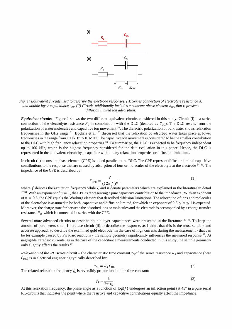
Equivalent circuits - Figure 1 shows the two different equivalent circuits considered in this study. Circuit (i) is a series

connection of the electrolyte resistance 𝑅s in combination with the DLC (denoted as 𝐶DL). The DLC results from the

polarization of water molecules and capacitive ion movement 30. The dielectric polarization of bulk water shows relaxation

frequencies in the GHz range 31. Bockris et al. 32 discussed that the relaxation of adsorbed water takes place at lower

frequencies in the range from 100 kHz to 10 MHz. The capacitive ion movement is considered to be the smaller contribution

to the DLC with high frequency relaxation properties 33. To summarize, the DLC is expected to be frequency independent

up to 100 kHz, which is the highest frequency considered for the data evaluation in this paper. Hence, the DLC is

represented in the equivalent circuit by a capacitor without any relaxation properties or diffusion limitations.

In circuit (ii) a constant phase element (CPE) is added parallel to the DLC. The CPE represent diffusion limited capacitive

contributions to the response that are caused by adsorption of ions or molecules of the electrolyte at the electrode 34–36. The

impedance of the CPE is described by

𝑍CPE =𝜁

(𝑖 2π 𝑓 )𝑛 ,

(1)

where 𝑓 denotes the excitation frequency while 𝜁 and 𝑛 denote parameters which are explained in the literature in detail 37,38. With an exponent of 𝑛 = 1, the CPE is representing a pure capacitive contribution to the impedance. With an exponent

of 𝑛 = 0.5, the CPE equals the Warburg element that described diffusion limitations. The adsorption of ions and molecules

of the electrolyte is assumed to be both, capacitive and diffusion limited, for which an exponent of 0.5 ≤ 𝑛 ≤ 1 is expected.

Moreover, the charge transfer between the adsorbed ions or molecules and the electrode is accompanied by a charge transfer

resistance 𝑅ct which is connected in series with the CPE.

Several more advanced circuits to describe double layer capacitances were presented in the literature 39–41. To keep the

amount of parameters small I here use circuit (ii) to describe the response, as I think that this is the most suitable and

accurate approach to describe the examined gold electrode. In the case of high currents during the measurement - that can

be for example caused by Faradaic reactions - the sample geometry significantly influences the measured response 42. At

negligible Faradaic currents, as in the case of the capacitance measurements conducted in this study, the sample geometry

only slightly affects the results 42.

Relaxation of the RC series circuit –The characteristic time constant 𝜏S of the series resistance 𝑅𝑆 and capacitance (here

𝐶DL) is in electrical engineering typically described by:

𝜏S = 𝑅𝑆 𝐶DL (2)

The related relaxation frequency 𝑓S is reversibly proportional to the time constant:

𝑓S =1

2𝜋 𝜏S

(3)

At this relaxation frequency, the phase angle as a function of log(𝑓) undergoes an inflection point (at 45° in a pure serial

RC-circuit) that indicates the point where the resistive and capacitive contributions equally affect the impedance.

Fig. 1: Equivalent circuits used to describe the electrode responses. (i): Series connection of electrolyte resistance 𝑅𝑠

and double layer capacitance 𝐶𝐷𝐿. (ii) Circuit additionally includes a constant phase element 𝑍𝐶𝑃𝐸 that represents

diffusion limited ion adsorption.

4 Results In the following, the measured and modeled responses of the examined smooth and porous gold electrode are presented.

Cyclic voltammetry measurements of the gold electrodes between 0 and 1.2 V vs RHE (see SI) showed the lowest amount

of Faradaic currents in the region around 0.5 V vs RHE. Accordingly, this potential was used as the mean electrode potential

for all conducted measurements.

The modeled electrode responses to sinusoidal excitations (impedance measurements) are calculated analytically, while

those to triangular excitations (cyclic voltammetry) are modeled numerically. Detailed mathematical descriptions of the

equivalent circuits are given in the SI. The equivalent circuits are parameterized based on the measured impedance spectra

as summarized in Table 1. A peak-to-peak amplitude 𝑈0 of 10 mV is used for cyclic voltammetry and impedance

measurements. This small excitation amplitude shall avoid potential driven contributions of Faradaic reactions.

To describe cyclic voltammetry measurements, the current 𝐼 is normalized to the employed scan rate:

𝐶𝑎𝑝 =𝐼

𝜈

(4)

Using this expression, the normalized current 𝐶𝑎𝑝 shows the dimension of capacitance (unit Farad). When capacitive

contributions dominate the response of an electrode during cyclic voltammetry, the normalized current 𝐶𝑎𝑝 equals its

capacitance. For interest readers, the physical response of the circuits graphed in Fig. 1 to triangular excitations is discussed

in the appendix in detail.

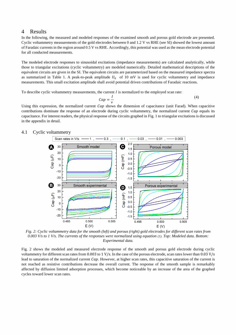
4.1 Cyclic voltammetry

Fig. 2: Cyclic voltammetry data for the smooth (left) and porous (right) gold electrodes for different scan rates from

0.003 V/s to 1 V/s. The currents of the responses were normalized using equation (1). Top: Modeled data. Bottom:

Experimental data.

Fig. 2 shows the modeled and measured electrode response of the smooth and porous gold electrode during cyclic

voltammetry for different scan rates from 0.003 to 1 V/s. In the case of the porous electrode, scan rates lower than 0.03 V/s

lead to saturation of the normalized current 𝐶𝑎𝑝. However, at higher scan rates, this capacitive saturation of the current is

not reached as resistive contributions decrease the overall current. The response of the smooth sample is remarkably

affected by diffusion limited adsorption processes, which become noticeable by an increase of the area of the graphed

cycles toward lower scan rates.

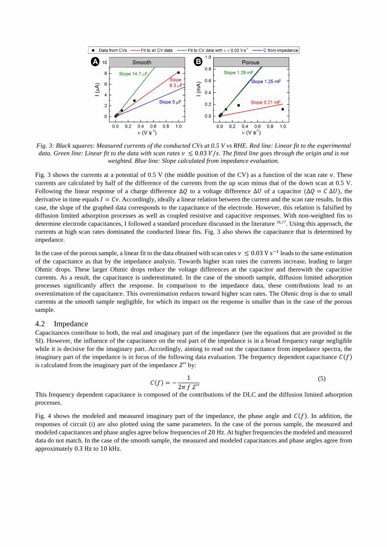
Fig. 3: Black squares: Measured currents of the conducted CVs at 0.5 V vs RHE. Red line: Linear fit to the experimental

data. Green line: Linear fit to the data with scan rates 𝜈 ≤ 0.03 𝑉/𝑠. The fitted line goes through the origin and is not

weighted. Blue line: Slope calculated from impedance evaluation.

Fig. 3 shows the currents at a potential of 0.5 V (the middle position of the CV) as a function of the scan rate 𝜈. These

currents are calculated by half of the difference of the currents from the up scan minus that of the down scan at 0.5 V.

Following the linear response of a charge difference Δ𝑄 to a voltage difference Δ𝑈 of a capacitor (Δ𝑄 = 𝐶 Δ𝑈), the

derivative in time equals 𝐼 = 𝐶𝜈. Accordingly, ideally a linear relation between the current and the scan rate results. In this

case, the slope of the graphed data corresponds to the capacitance of the electrode. However, this relation is falsified by

diffusion limited adsorption processes as well as coupled resistive and capacitive responses. With non-weighted fits to

determine electrode capacitances, I followed a standard procedure discussed in the literature 16,17. Using this approach, the

currents at high scan rates dominated the conducted linear fits. Fig. 3 also shows the capacitance that is determined by

impedance.

In the case of the porous sample, a linear fit to the data obtained with scan rates ν ≤ 0.03 V s−1 leads to the same estimation

of the capacitance as that by the impedance analysis. Towards higher scan rates the currents increase, leading to larger

Ohmic drops. These larger Ohmic drops reduce the voltage differences at the capacitor and therewith the capacitive

currents. As a result, the capacitance is underestimated. In the case of the smooth sample, diffusion limited adsorption

processes significantly affect the response. In comparison to the impedance data, these contributions lead to an

overestimation of the capacitance. This overestimation reduces toward higher scan rates. The Ohmic drop is due to small

currents at the smooth sample negligible, for which its impact on the response is smaller than in the case of the porous

sample.

4.2 Impedance Capacitances contribute to both, the real and imaginary part of the impedance (see the equations that are provided in the

SI). However, the influence of the capacitance on the real part of the impedance is in a broad frequency range negligible

while it is decisive for the imaginary part. Accordingly, aiming to read out the capacitance from impedance spectra, the

imaginary part of the impedance is in focus of the following data evaluation. The frequency dependent capacitance 𝐶(𝑓)

is calculated from the imaginary part of the impedance 𝑍′′ by:

𝐶(𝑓) = −1

2𝜋 𝑓 𝑍′′

(5)

This frequency dependent capacitance is composed of the contributions of the DLC and the diffusion limited adsorption

processes.

Fig. 4 shows the modeled and measured imaginary part of the impedance, the phase angle and 𝐶(𝑓). In addition, the

responses of circuit (i) are also plotted using the same parameters. In the case of the porous sample, the measured and

modeled capacitances and phase angles agree below frequencies of 20 Hz. At higher frequencies the modeled and measured

data do not match. In the case of the smooth sample, the measured and modeled capacitances and phase angles agree from

approximately 0.3 Hz to 10 kHz.

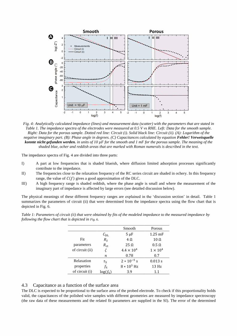
Fig. 4: Analytically calculated impedance (lines) and measurement data (scatter) with the parameters that are stated in

Table 1. The impedance spectra of the electrodes were measured at 0.5 V vs RHE. Left: Data for the smooth sample.

Right: Data for the porous sample. Dotted red line: Circuit (i). Solid black line: Circuit (ii). (A): Logarithm of the

negative imaginary part. (B): Phase angle in degrees. (C) Capacitances calculated by equation Fehler! Verweisquelle

konnte nicht gefunden werden. in units of 10 µF for the smooth and 1 mF for the porous sample. The meaning of the

shaded blue, ocher and reddish areas that are marked with Roman numerals is described in the text.

The impedance spectra of Fig. 4 are divided into three parts:

I) A part at low frequencies that is shaded blueish, where diffusion limited adsorption processes significantly

contribute to the impedance.

II) The frequencies close to the relaxation frequency of the RC series circuit are shaded in ochery. In this frequency

range, the value of 𝐶(𝑓) gives a good approximation of the DLC.

III) A high frequency range is shaded reddish, where the phase angle is small and where the measurement of the

imaginary part of impedance is affected by large errors (see detailed discussion below).

The physical meanings of these different frequency ranges are explained in the ‘discussion section’ in detail. Table 1

summarizes the parameters of circuit (ii) that were determined from the impedance spectra using the flow chart that is

depicted in Fig. 6.

Table 1: Parameters of circuit (ii) that were obtained by fits of the modeled impedance to the measured impedance by

following the flow chart that is depicted in Fig. 6.

Smooth Porous 𝐶DL 5 μF 1.25 mF

Fit 𝑅𝑆 4 Ω 10 Ω

parameters 𝑅ct 25 Ω 0.5 Ω

of circuit (ii) 𝜁 4.4 × 104 1 × 104 𝑛 0.78 0.7

Relaxation 𝜏S 2 ∗ 10−5 s 0.013 s

properties 𝑓S 8 ∗ 103 Hz 13 Hz

of circuit (i) log (𝑓S) 3.9 1.1

4.3 Capacitance as a function of the surface area The DLC is expected to be proportional to the surface area of the probed electrode. To check if this proportionality holds

valid, the capacitances of the polished wire samples with different geometries are measured by impedance spectroscopy

(the raw data of these measurements and the related fit parameters are supplied in the SI). The error of the determined

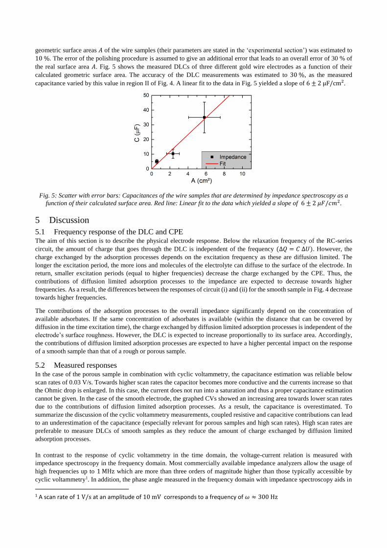
geometric surface areas 𝐴 of the wire samples (their parameters are stated in the ‘experimental section’) was estimated to

10 %. The error of the polishing procedure is assumed to give an additional error that leads to an overall error of 30 % of

the real surface area 𝐴. Fig. 5 shows the measured DLCs of three different gold wire electrodes as a function of their

calculated geometric surface area. The accuracy of the DLC measurements was estimated to 30 %, as the measured

capacitance varied by this value in region II of Fig. 4. A linear fit to the data in Fig. 5 yielded a slope of 6 ± 2 μF/cm².

Fig. 5: Scatter with error bars: Capacitances of the wire samples that are determined by impedance spectroscopy as a

function of their calculated surface area. Red line: Linear fit to the data which yielded a slope of 6 ± 2 𝜇𝐹/𝑐𝑚2.

5 Discussion

5.1 Frequency response of the DLC and CPE The aim of this section is to describe the physical electrode response. Below the relaxation frequency of the RC-series

circuit, the amount of charge that goes through the DLC is independent of the frequency (Δ𝑄 = 𝐶 Δ𝑈). However, the

charge exchanged by the adsorption processes depends on the excitation frequency as these are diffusion limited. The

longer the excitation period, the more ions and molecules of the electrolyte can diffuse to the surface of the electrode. In

return, smaller excitation periods (equal to higher frequencies) decrease the charge exchanged by the CPE. Thus, the

contributions of diffusion limited adsorption processes to the impedance are expected to decrease towards higher

frequencies. As a result, the differences between the responses of circuit (i) and (ii) for the smooth sample in Fig. 4 decrease

towards higher frequencies.

The contributions of the adsorption processes to the overall impedance significantly depend on the concentration of

available adsorbates. If the same concentration of adsorbates is available (within the distance that can be covered by

diffusion in the time excitation time), the charge exchanged by diffusion limited adsorption processes is independent of the

electrode’s surface roughness. However, the DLC is expected to increase proportionally to its surface area. Accordingly,

the contributions of diffusion limited adsorption processes are expected to have a higher percental impact on the response

of a smooth sample than that of a rough or porous sample.

5.2 Measured responses In the case of the porous sample in combination with cyclic voltammetry, the capacitance estimation was reliable below

scan rates of 0.03 V/s. Towards higher scan rates the capacitor becomes more conductive and the currents increase so that

the Ohmic drop is enlarged. In this case, the current does not run into a saturation and thus a proper capacitance estimation

cannot be given. In the case of the smooth electrode, the graphed CVs showed an increasing area towards lower scan rates

due to the contributions of diffusion limited adsorption processes. As a result, the capacitance is overestimated. To

summarize the discussion of the cyclic voltammetry measurements, coupled resistive and capacitive contributions can lead

to an underestimation of the capacitance (especially relevant for porous samples and high scan rates). High scan rates are

preferable to measure DLCs of smooth samples as they reduce the amount of charge exchanged by diffusion limited

adsorption processes.

In contrast to the response of cyclic voltammetry in the time domain, the voltage-current relation is measured with

impedance spectroscopy in the frequency domain. Most commercially available impedance analyzers allow the usage of

high frequencies up to 1 MHz which are more than three orders of magnitude higher than those typically accessible by

cyclic voltammetry1. In addition, the phase angle measured in the frequency domain with impedance spectroscopy aids in

1 A scan rate of 1 V/s at an amplitude of 10 mV corresponds to a frequency of 𝜔 ≈ 300 Hz

the data evaluation. With reference to these advantages of impedance spectroscopy, this technique is from now on in focus

of the discussion. In the case of circuit (ii), the DLC and the diffusion limited adsorption processes both affect the imaginary

part of the impedance. Both contributions can only be separated by a detailed evaluation of the frequency response that is

discussed in the following.

5.3 Impedance evaluation and capacitance determination During high frequency probing of circuit (i) or (ii), the phase angle approaches zero as the impedance of the capacitor and

CPE both decrease and thus the contribution of the electrolyte resistance dominates. The imaginary part of the impedance

is calculated from the measured total impedance 𝑍 and the phase angle 𝜃 by 𝑍′′ = 𝑍 sin (𝜃). At small values of 𝜃, the

approximation sin(𝜃) ≈ 𝜃 is valid, which means that the measurement error of 𝜃 directly affects the error of the imaginary

part of the impedance. For example, if 𝜃 = 2° ± 1°, the relative error of 𝑍′′ is ± 50 %, while in the case of 𝜃 = 45° ± 1°

the error of 𝑍′′ is negligible. Accordingly, the relative measurement error of 𝑍′′ increases towards a low absolute value of

the phase angle. Moreover, inductive contributions affect 𝑍′′ linearly with frequency and are thus complicating the

capacitance estimation. The frequency range where these effects significantly falsify the measurements was shaded reddish

in Fig. 4 and shall not be used for a proper impedance analysis. The impedance measurements are reliable at phase angles

above 5°.

Based on the previous paragraph and Section 5.1, the following two facts can be condensed:

1) The higher the frequency, the smaller are the contributions of diffusion limited adsorption processes.

2) The smaller the phase angle, the higher is the measurement error of the imaginary part.

With reference to these trends, I propose that the frequency region around the relaxation of the series circuit is best to read

out the DLC from impedance spectra. In this frequency region, the absolute value of the phase angle is large enough to

enable a precise determination of the imaginary part of the impedance, while adsorption processes ideally have a negligible

proportion on the measured response. If diffusion limited adsorption processes are near the relaxation frequency negligible,

both, circuit (i) and (ii) have the same relaxation frequency. If not, it is not possible to distinguish between the contributions

of the DLC and diffusion limited adsorption processes, as further discussed in the following.

In the ‘theory section’ I discussed that the relaxation frequency 𝑓S of the RC series circuit equals the high frequency

inflection point 𝑓ip of the phase angle. The CPE can shift the inflection point 𝑓ip of the phase angle toward lower values

than the 45° of a pure RC-series circuit. The examined gold electrodes showed 𝑓ip between 30° and 45°. The relaxation

frequency 𝑓S of the series circuit can be calculated by equation (3). The electrolyte resistance 𝑅S typically equals the real

part of the impedance at 100 kHz, for which it is often referred to as high frequency resistance. Ideally, 𝑓ip and 𝑓S should

exactly match, which means that 𝐶ip equals the double layer capacitance 𝐶DL. The percental difference of 𝑓ip and 𝑓𝑆 can be

used as a measure for the relative error of the capacitance estimation:

Δ𝐶DL = 𝐶ip

(𝑓ip − 𝑓𝑆)

𝑓𝑆

(6)

However, the values of 𝑓ip and 𝑓S are themselves typically accompanied by large errors, which complicate a precise error

estimation by the latter equation. Nevertheless, the latter equation is an easy approach to control whether the estimated

capacitance is in the right order of magnitude. Generally, the influence of diffusion limited adsorption processes increases

the value of Δ𝐶DL. With reference to the discussed samples, the values of 𝑓𝑆 of the probed electrodes summarized in Table

1 agree well with the values of 𝑓ip in Fig. 4.

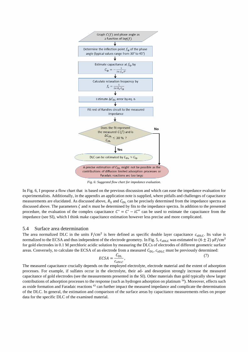
Fig. 6: Suggested flow chart for impedance evaluation.

In Fig. 6, I propose a flow chart that is based on the previous discussion and which can ease the impedance evaluation for

experimentalists. Additionally, in the appendix an application note is supplied, where pitfalls and challenges of capacitance

measurements are elucidated. As discussed above, 𝑅S and 𝐶DL can be precisely determined from the impedance spectra as

discussed above. The parameters 𝜁 and 𝑛 must be determined by fits to the impedance spectra. In addition to the presented

procedure, the evaluation of the complex capacitance 𝐶∗ = 𝐶′ − 𝑖𝐶′′ can be used to estimate the capacitance from the

impedance (see SI), which I think make capacitance estimation however less precise and more complicated.

5.4 Surface area determination The area normalized DLC in the units F/cm2 is here defined as specific double layer capacitance 𝑐sDLC. Its value is

normalized to the ECSA and thus independent of the electrode geometry. In Fig. 5, 𝑐sDLC was estimated to (6 ± 2) μF/cm²

for gold electrodes in 0.1 M perchloric acidic solution by measuring the DLCs of electrodes of different geometric surface

areas. Conversely, to calculate the ECSA of an electrode from a measured 𝐶DL, 𝑐sDLC must be previously determined:

𝐸𝐶𝑆𝐴 =𝐶DL

𝑐sDLC

, (7)

The measured capacitance crucially depends on the employed electrolyte, electrode material and the extent of adsorption

processes. For example, if sulfates occur in the electrolyte, their ad- and desorption strongly increase the measured

capacitance of gold electrodes (see the measurements presented in the SI). Other materials than gold typically show larger

contributions of adsorption processes to the response (such as hydrogen adsorption on platinum 34). Moreover, effects such

as oxide formation and Faradaic reactions 43 can further impact the measured impedance and complicate the determination

of the DLC. In general, the estimation and comparison of the surface areas by capacitance measurements relies on proper

data for the specific DLC of the examined material.

6 Conclusions In this study, comparative capacitance measurements of gold electrodes in perchloric acid are conducted using cyclic

voltammetry and impedance spectroscopy. The measured responses are described by physical models. Besides the double

layer capacitance (DLC), diffusion limited adsorption processes affect the response. Towards higher frequencies, the

impact of the diffusion limited adsorption processes on the impedance decrease. Using impedance spectroscopy, higher

frequencies are accessible comparable to cyclic voltammetry. Another advantage of impedance spectroscopy is that serial

resistive and capacitive contributions can be separated with the information carried by the phase angle. I derive that the

relaxation frequency of the RC-series circuit can be used to survey the validity of the DLC estimation. By examining gold

electrodes of different defined geometric surfaces, a linear relation between the surface area and measured capacitance is

shown. Values for the specific DLC of gold electrodes in perchloric acid reported previously were often overestimated, as

they were determined at low frequencies, where diffusion limited adsorption processes dominated the response. I propose

a handy flow chart that describes how to extract capacitances from impedance spectra and how to use the relaxation

frequency to survey the error of the determined DLC of a sample.

7 Nomenclature 𝐶(𝑓) Capacitance calculated by eq. 5 (F)

𝐶𝑎𝑝 Capacitance calculated by eq. 4 (F)

𝐶DL Double layer capacitance (F)

𝐶ip Capacitance at the inflection point of the phase angle (F)

𝑐sDLC Specific capacitance (F cm−2)

Δ𝐶DL Error of the double layer capacitance estimation (F)

𝐸𝐶𝑆𝐴 Electrochemically active surface area (m2)

𝑓 Frequency (Hz)

𝑓ip Frequency of the inflection point in the phase angle (Hz)

𝑓S Relaxation frequency of the RC-series circuit (Hz)

𝑖 Complex number

𝐼 Current (A)

𝑛 Constant phase element parameter (dimensionless)

Δ𝑄 Charge difference (C)

𝑅ct Charge transfer resistance (Ω)

𝑅S Electrolyte or serial resistance (Ω)

Δ𝑈 Voltage difference (V)

𝑈0 Excitation amplitude (V)

𝑍 Impedance (Ω)

𝑍′ Real part of impedance (Ω)

𝑍′′ Imaginary part of impedance (Ω)

𝑍CPE Constant phase element (Ω)

𝜃 Phase angle

𝜁 Constant phase element parameter (cm)

𝜏S Relaxation time of the RC-series circuit (s)

𝜏ct Relaxation time of the RC-parallel circuit (s)

𝜈 Scan rate (V/s)

8 References 1. P. Quaino, F. Juarez, E. Santos, and W. Schmickler, Beilstein J. Nanotechnol., 5, 846–854 (2014).

2. I. Katsounaros, S. Cherevko, A. R. Zeradjanin, and K. J. J. Mayrhofer, Angew. Chem. Int. Ed. Engl., 53, 102–21

3. M. Schalenbach et al., J. Electrochem. Soc., 163, F3197–F3208 (2016).

4. M. Schalenbach, A. R. Zeradjanin, O. Kasian, S. Cherevko, and K. J. J. Mayrhofer, Int. J. Electrochem. Sci., 13, 1173–

5. G. Jarzabek and Z. Borkowska, Electrochim. Acta, 42, 2915–2918 (1997).

6. M. Watt-Smith, J. Friedrich, S. Rigby, T. Ralph, and F. Walsh, J. Phys. D Appl. Phys., 41, 1–8 (2008).

7. S. Trasatti and O. A. Petrii, J. Electroanal. Chem., 327, 353–376 (1992).

8. D. S. Hall, C. Bock, and B. R. MacDougall, J. Electrochem. Soc., 161, H787–H795 (2014)

9. E. Herrero, L. J. Buller, and H. D. Abruna, Chem. Rev., 101, 1897–1930 (2001)

10. U. Heiz, A. Sanchez, S. Abbet, and W. Schneider, J. Am. Chem. Soc., 121, 3214–3217 (1999).

11. J. M. Doña Rodríguez, J. A. Herrera Melián, and J. Pérez Peña, J. Chem. Educ., 77, 1195–1197 (2000)

12. S. M. Alia, K. E. Hurst, S. S. Kocha, and B. S. Pivovar, J. Electrochem. Soc., 163, F3051–F3056 (2016).

13. M. Schalenbach et al., Electrochim. Acta, 259, 1154–1161 (2017).

14. K. S. W. Sing, Adv. Colloid Interface Sci., 76–77, 3–11 (1998)

15. S. Brunauer, P. H. Emmett, and E. Teller, J. Am. Chem. Soc., 60, 309–319 (1938)

16. C. C. L. McCrory et al., J. Am. Chem. Soc., 137, 4347–4357 (2015) http://pubs.acs.org/doi/abs/10.1021/ja510442p.

17. C. C. L. McCrory, S. Jung, J. C. Peters, and T. F. Jaramillo, J. Am. Chem. Soc., 135, 16977–16987 (2013).

18. S. Jung, C. C. L. McCrory, I. M. Ferrer, J. C. Peters, and T. F. Jaramillo, J. Mater. Chem. A, 4, 3068–3076 (2016)

19. B. Hammer and J. K. Norskov, Nature, 376, 238–240 (1995).

20. B. Piela and P. Wrona, J. Electroanal. Chem., 388, 69–79 (1995).

21. A. J. Motheo, A. Sadkowski, and R. S. Neves, J. Electroanal. Chem., 430, 253–262 (1997).

22. A. J. Motheo, J. R. Santos, A. Sadkowski, and A. Hamelin, J. Electroanal. Chem., 397, 331–334 (1995).

23. T. Pajkossy, Solid State Ionics, 94, 123–129 (1997).

24. T. Pajkossy, Solid State Ionics, 176, 1997–2003 (2005).

25. G. M. Schmid and N. Hackerman, J. Electrochem. Soc., 109, 243–247 (1962)

26. B. B. Berkes, A. Maljusch, W. Schuhmann, and A. S. Bondarenko, J. Phys. Chem. C, 115, 9122–9130 (2011).

27. G. J. Brug, A. L. G. van den Eeden, M. Sluyters-Rehbach, and J. H. Sluyters, J. Electroanal. Chem., 176, 275–295

(1984).

28. M. E. Abdelsalam, P. N. Bartlett, T. Kelf, and J. Baumberg, Langmuir, 21, 1753–1757 (2005).

29. S. Cherevko and C. H. Chung, Electrochem. commun., 13, 16–19 (2011)

30. E. Spohr, Electrochim. Acta, 49, 23–27 (2003).

31. U. Kaatze, J. Solution Chem., 26, 1049–1112 (1997) http://link.springer.com/10.1007/BF02768829.

32. J. Bockris, E. Gileadi, and K. Mueller, J. Chem. Phys., 44, 1445–1456 (1966)

33. C. H. Hamann, A. Hamnett, and W. Vielstich, Electrochemistry, 2nd ed., Wiley-VCH, (2007).

34. A. Tymosiak-Zielińska and Z. Borkowska, Electrochim. Acta, 46, 3063–3071 (2001).

35. D. Leikis, K. Rybalka, E. Sevatyanov, and A. Frumkin, Electroanal. Chem. Interfacial Electrochem., 46, 161–169

(1973).

36. W. G. Pell, A. Zolfaghari, and B. E. Conway, J. Electroanal. Chem., 532, 13–23 (2002).

37. J.-B. Jorcin, M. E. Orazem, N. Pébère, and B. Tribollet, Electrochim. Acta, 51, 1473–1479 (2006).

38. P. Zoltowski, Electroanal. Chem., 443, 149–154 (1998).

39. J. Kang, J. Wen, S. H. Jayaram, A. Yu, and X. Wang, Electrochim. Acta, 115, 587–598 (2014)

40. H. Wang and L. Pilon, Electrochim. Acta, 64, 130–139 (2012) http://dx.doi.org/10.1016/j.electacta.2011.12.118.

41. H. Wang, A. Thiele, and L. Pilon, J. Phys. Chem. C, 117, 18286–18297 (2013).

42. V. M.-W. Huang, V. Vivier, M. E. Orazem, N. Pebere, and B. Tribollet, J. Electrochem. Soc., 154, C99 (2007).

43. T. Brousse, D. Belanger, and J. W. Long, J. Electrochem. Soc., 162, A5185–A5189 (2015)

44. R. Makharia, M. F. Mathias, and D. R. Baker, J. Electrochem. Soc., 152, A970 (2005)

45. J. Bisquert, Phys. Chem. Chem. Phys, 2, 4185–4192 (2000).

46. U. Rammelt and G. Reinhard, Electrochim. Acta, 35, 1045–1049 (1990).

47. H. Song et al., Electrochim. Acta, 44, 3513–3519 (1999).

9 Appendix The appendix contains:

• Application notes for experimentalists displaying pitfalls and limitations to measure the DLC & ECSA via

capacitance.

• A detail description of the analytical and numerical model that was used to describe the measurements.

• An example how the resistors and capacitor affect the response of cyclic voltammetry measurements.

• Relaxation properties of the RC-parallel circuit

• Examinations on the measurement precision with dummy cells that consist of the same parameters as the

equivalent circuit diagrams used for the measurements.

• Comparative measurements on a plane electrode that show a negligible impact of sample geometry on the

presented results.

• Raw data of the gold-wire measurements that are displayed in Fig. 5.

• Capacitance measurements at different potentials

• Measurements of the smooth gold electrode in sulfuric acid

• CV data between 0 and 1.2 V vs RHE

• Limitations of impedance measurements

• Impedance data graphed as complex capacitance

9.1 Application Notes I like to present the following suggestions to measure the surface area and double layer capacitances of electrodes:

1) Setup: Special care should be given to the choice of the electrolyte, as different ion species can significantly affect the

contributions of adsorption processes to the measured response (see example of Au electrode with sulfates below).

The electrolyte should be purged with non-reactive gases such as argon or nitrogen in order to avoid electrochemical

reactions related to reactive gases such as atmospheric oxygen. The distance of the Luggin capillary to the working

electrode should be as small as possible to achieve a small value of the electrolyte resistance2. If a sample is supported

by an additional conductive material (as for instance carbon), both materials will contribute to the measured

capacitance.

2) Measurement procedure: I suggest to rather use impedance spectroscopy than cyclic voltammetry for capacitance

measurements with reference to the discussion presented in the article. The quality of impedance analyzers should be

examined to check whether the used device enables a trustworthy determination of the capacitance3. The measured

2 The smaller the value of 𝑅S, the higher is the relaxation frequency of the RC series circuit and the lower is the impact of adsorption processes at this frequency. Thus, small values of 𝑅S ease the capacitance determination. 3 In the relevant region of the relaxation of the RC series circuit, the value of the impedance is typically in the order of a

few Ohms. Under these conditions, the measurement error of impedance analyzers are typically quite large. Dummy

capacitance can significantly depend on the potential especially when ad- or desorption phenomena contribute. Thus,

I recommend to measure the capacitance at various electrode potentials. Cyclic voltammetry however can be useful to

measure samples with capacitances higher than 1 mF, which can lead to relaxation frequencies that can be lower that

the available spectrum of impedance analyzers. Capacitance measurements by cyclic voltammetry are in our opinion

only suitable if the determined capacitance is independent within at least tenfold different values of the scan rate.

3) Impedance evaluation: The flow chart that I presented might be a simple and appropriate procedure to extract

capacitances from impedance spectra. If an equivalent circuit diagram to fit a function to the measured data is used,

this should not be too complex, as with a high amount of parameters arbitrary functions can be drawn but the physical

meaning of the parameters can be lost.

4) Pitfalls and limits: If the sample has pores or if the distance to the counter electrode varies, the Ohmic drop can lead

to inhomogeneous potential differences between the electrode and the electrolyte 44. These differences are attributable

to Ohmic drops resulting from the ionic conduction through the pores. In addition, bad conducting electrodes (such as

oxides) can lead to significant potential drop in the electrode itself. In these cases, the equivalent circuit diagram

consists of additional constant phase elements 37,45–47. Thus, the values of the resistances and the extent of diffusion

limitations are decisive, whether the capacitance can be read out correctly from the measured impedance. In the case

of 𝑅ct ≫ 𝑅S, the capacitance can be read out by flow chart presented as the RC series circuit dominates the measured

response. If 𝑅ct is equal or smaller than 𝑅S , redox processes can overshadow the impact of the capacitance on the

impedance. However, in the case of strongly diffusion limited redox processes it still may be possible to estimate the

capacitance from the impedance spectra.

5) Surface area estimation: The specific capacitance of the electrode and electrolyte combination should be measured

with a smooth sample of a defined surface area, as comparing the capacitances of different electrode materials can

lead to wrong estimations of the surface area.

9.2 General comments for the model The response of the circuit (ii) to sinosoidal excitations that are applied during impedance spectroscopy can be easily

described by an analytical solution. However, its responses to the triangular excitations that are applied during cyclic

voltammetry are difficult to describe by an analytical solution and thus are treated by an easier numerical solution. For all

the model descriptions considered, Ohmic drops at resistors are described by Ohms law:

The capacitances are characterized by a linear response of the change of charge Δ𝑄 to a potential alteration of Δ𝑈𝐶. The

capacitance 𝐶 connects both properties:

Δ𝑄 = 𝐶 Δ𝑈𝐶 (9)

9.3 Analytical model for the impedance

9.3.1 Analytical description

The analytical solution of the impedance for circuit (ii) is rigorously discussed in the literature and is thus only briefly

reviewed in the following. For the purpose of simplification, the angular frequency 𝜔 = 2𝜋𝑓 is introduced. The impedance

of circuit (ii) equals:

𝑍 = 𝑅s +1

(𝑅ct + 𝑍CPE)−1 + 𝑖𝜔𝐶DL

(10)

The impedance of the CPE (denotes as 𝑍CPE) is typically described by

𝑍CPE =𝜁

(𝑖𝜔)𝑛 ,

(11)

where 𝜁 and 𝑛 denote the parameters that characterize the CPE. For the sake of simplification, the parameter 𝑛 is in the

following substitute by 𝑛 = −𝛼:

𝑍CPE = 𝜁 (𝑖𝜔)𝛼 (12)

By making use of the Euler equation, the latter equation can be rewritten as:

𝑍CPE = 𝜁 𝜔𝛼⌊cos(0.5 𝜋𝛼) + 𝑖 sin(0.5 𝜋𝛼)⌋ (13)

The following abbreviations are used to ease the calculations below:

𝜌 = 𝑅𝑒(𝑍CPE) = 𝜁 cos(0.5 𝜋𝛼) 𝜔𝛼 (14)

𝜎 = 𝐼𝑚(𝑍CPE) = 𝜁 sin(0.5 𝜋𝛼) 𝜔𝛼 (15)

By setting equation (13) into equation (10), the real and imaginary part of the impedance can be calculated to

cells that consist of electric resistances and capacitors with the same resistances and capacitances as those of the

measured electrochemical cell are effective approaches to characterize the measurement precision (see below).

𝑈 = 𝑅 𝐼 (8)

𝑍′ = 𝑅s +𝛽

𝛽2 + 𝛾2

(16)

−𝑍′′ =𝛾

𝛽2 + 𝛾2 , (17)

where 𝛽 and 𝛾 represent the following terms:

𝛽 =(𝑅ct + 𝜌)

(𝑅ct + 𝜌)2 + 𝜎2

(18)

𝛾 = −𝜎

(𝑅ct + 𝜌)2 + 𝜎2+ 𝜔𝐶DL . (19)

9.3.2 Fit function for the capacitance

Using the relation

C(ω) = −1

𝜔 𝑍′′=

𝛽2 + 𝛾2

𝜔 𝛾 ,

(20)

the fit function for the frequency dependent capacitance C(ω) can be derived to:

C(ω) = 𝐶DL +

1𝜔

− 𝐶DL 𝜉 sin (𝜋𝛼2

) 𝜔𝛼

−𝜉 sin (𝜋𝛼2

) 𝜔𝛼 + [(𝑅ct + 𝜉 cos (𝜋𝛼2

) 𝜔𝛼 )2

+ (𝜉 sin (𝜋𝛼2

) 𝜔𝛼 )2

] 𝜔𝐶DL

(21)

9.3.3 Relaxation time of the RC-parallel circuit

Debye derived an analytical equation to describe the complex dielectric function of solids and their relaxation. This

expression can be transferred to the relaxation of the RC-parallel circuit, while the corresponding relaxation time is here

denoted as 𝜏ct. For the purpose of simplification the CPE is neglected now. Using the equation

which is similar to the equation that was derived by Debye, an equivalent description of the impedance in terms of equation

(10) with a negligible CPE (𝜉 = 0) can be provided. When the angular frequency times the relaxation time equals unity

(𝜔𝜏ct = 1), the imaginary part of the impedance shows a maximum while the phase angle shows a minimum. This extreme

means d𝑍′′

dω= 0. Based on this relation the relaxation time of the RC parallel circuit can be calculated to:

𝜏ct = 𝑅ct 𝐶DL . (23)

9.3.4 Relation of relaxation time and inflection point of the phase angle

As discussed in the article, the frequency of the inflection point 𝑓ip of the phase angle should equal the relaxation frequency

𝑓s of the serial 𝑅𝐶-circuit to enable a proper capacitance estimation. This relation is displayed in Fig. S7 for the parameters

of the smooth sample with a variation of the capacitance from 0.5 to 50 μF. In Fig. S7A, the ratio of 𝑓s to 𝑓 is displayed,

as calculated by 𝑓s

𝑓=

1

2𝜋 𝑓 𝑅s 𝐶DL. The ratio equals unity when 𝑓 = 𝑓s. At this frequency the phase angle undergoes the

inflection point 𝑓ip of the phase angle. Moreover, at this frequency, the relation 𝐶(𝑓) ≈ 𝐶DL is typically reached, which

means that the frequency dependent capacitance shows almost the same value as the sample capacitance. The inflection

point 𝑓ip of the phase angle typically takes place between -35° and -45°. In general, higher capacitances decrease the

relaxation frequency of the 𝑅𝐶-circuit.

𝑍 = 𝑅E +𝑅ct

1 + 𝑖𝜔𝜏ct

, (22)

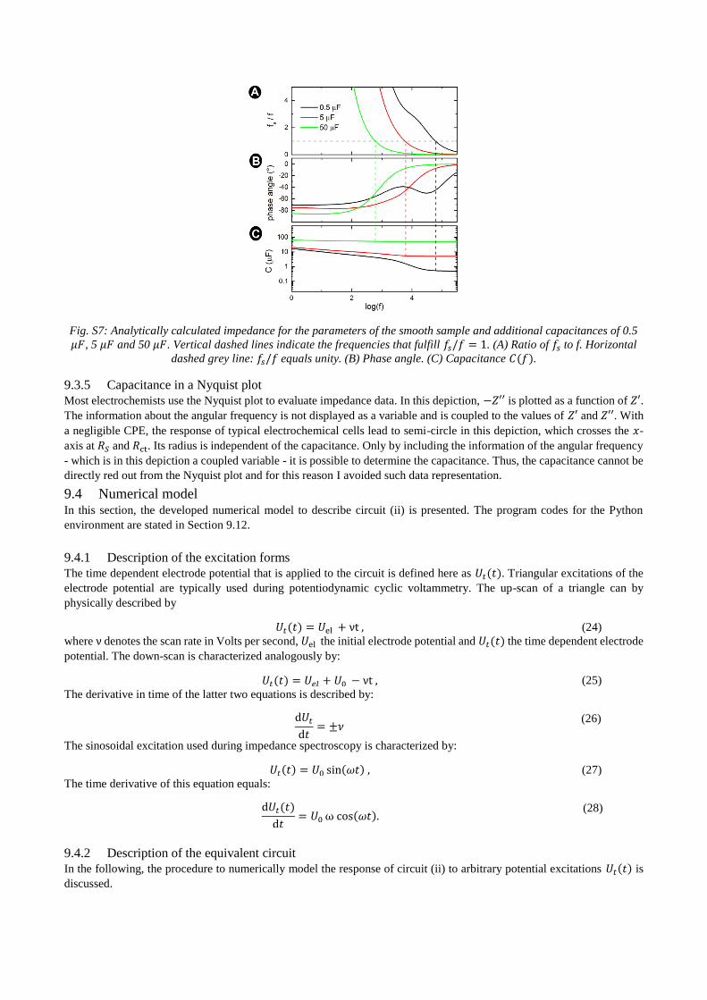
Fig. S7: Analytically calculated impedance for the parameters of the smooth sample and additional capacitances of 0.5

𝜇𝐹, 5 𝜇𝐹 and 50 𝜇𝐹. Vertical dashed lines indicate the frequencies that fulfill 𝑓𝑠/𝑓 = 1. (A) Ratio of 𝑓𝑠 to f. Horizontal

dashed grey line: 𝑓𝑠/𝑓 equals unity. (B) Phase angle. (C) Capacitance 𝐶(𝑓).

9.3.5 Capacitance in a Nyquist plot

Most electrochemists use the Nyquist plot to evaluate impedance data. In this depiction, −𝑍′′ is plotted as a function of 𝑍′.

The information about the angular frequency is not displayed as a variable and is coupled to the values of 𝑍′ and 𝑍′′. With

a negligible CPE, the response of typical electrochemical cells lead to semi-circle in this depiction, which crosses the 𝑥-

axis at 𝑅𝑆 and 𝑅ct. Its radius is independent of the capacitance. Only by including the information of the angular frequency

- which is in this depiction a coupled variable - it is possible to determine the capacitance. Thus, the capacitance cannot be

directly red out from the Nyquist plot and for this reason I avoided such data representation.

9.4 Numerical model In this section, the developed numerical model to describe circuit (ii) is presented. The program codes for the Python

environment are stated in Section 9.12.

9.4.1 Description of the excitation forms

The time dependent electrode potential that is applied to the circuit is defined here as 𝑈𝑡(𝑡). Triangular excitations of the

electrode potential are typically used during potentiodynamic cyclic voltammetry. The up-scan of a triangle can by

physically described by

𝑈𝑡(𝑡) = 𝑈el + νt , (24)

where ν denotes the scan rate in Volts per second, 𝑈el the initial electrode potential and 𝑈𝑡(𝑡) the time dependent electrode

potential. The down-scan is characterized analogously by:

𝑈𝑡(𝑡) = 𝑈𝑒𝑙 + 𝑈0 − νt , (25)

The derivative in time of the latter two equations is described by:

d𝑈𝑡

d𝑡= ±𝜈

(26)

The sinosoidal excitation used during impedance spectroscopy is characterized by:

𝑈𝑡(𝑡) = 𝑈0 sin(𝜔𝑡) , (27)

The time derivative of this equation equals:

d𝑈𝑡(𝑡)

d𝑡= 𝑈0 ω cos(𝜔𝑡).

(28)

9.4.2 Description of the equivalent circuit

In the following, the procedure to numerically model the response of circuit (ii) to arbitrary potential excitations 𝑈𝑡(𝑡) is

discussed.

Constant phase element (CPE) - The CPE equals the sum of an Ohmic part and a part that only contributes to imaginary

part of the current. Accordingly, the different contributions to the real and imaginary part of the current to the CPE can be

expressed by a series equivalent circuit of 𝑍CPE′ and 𝑍CPE′′:

𝑍CPE = 𝑍CPE′ + 𝑖𝑍CPE′′ (29)

The real part of the CPE equals the above defined 𝜌. Accordingly, the resistive current through the CPE can be calculated

by Ohm’s law:

𝑈CPE = 𝑍CPE′ 𝐼CPE = 𝜌 𝐼CPE (30)

The angular frequency is in the case of a triangular function not well defined and is replaced by expression that equals

the inverse period time times 2π:

=2π 𝜈

𝑈0

(31)

For the purpose of simplification, a sinusoidal excitation shall here be considered in order to describe the imaginary current.

In the following, 𝑈 denotes the voltage at the imaginary part of the CPE while 𝐼 denotes the capacitive current. When the

response of a pure imaginary impedance element contributes, the phase angle of the current is tilt by −90°. Accordingly,

in the case of 𝑈(𝑡) = 𝑈0 sin(𝜔𝑡), Ohm’s law for the imaginary part of the impedance can be written as:

𝑈0 sin(𝜔𝑡 − 𝜑) = 𝑍′′ 𝐼(𝑡) (32)

By using 𝜑 = −90° for a pure imaginary current, the relation sin(𝜔𝑡 − 𝜑) = −cos(𝜔𝑡) results. With the definition of the

imaginary part of the CPE, the latter equation can be rewritten as:

𝑈0 cos(𝜔𝑡) = −𝜎 𝐼(𝑡). (33)

Using the derivative of the 𝑈(𝑡) in time (as described by eq. (28)), this expression equals:

d

d𝑡𝑈(𝑡) = −𝜎 𝐼 .

(34)

The latter equation is a general description of the CPE and also can be used to describe triangular excitations. In total, the

real and imaginary part of the CPE are described on the basis of equation (30) and (34) by:

d

d𝑡𝑈𝑍CPE

(𝑡) = 𝜌d

d𝑡𝐼𝑍CPE

+ 𝜎 𝐼𝑍CPE ,

(35)

where 𝑈𝑍𝑊 and 𝐼𝑍𝑊

denote the overall voltage and current at the CPE.

Parallel circuit - To ease the physical description of circuit (ii) I like to first consider the parallel circuit. In this parallel

sub-circuit the series connection of the charge transfer resistance and the CPE is aligned parallel to the capacitor. The

current and voltage at the capacitor are defined by 𝑈𝐶 and 𝐼𝐶 . By taking the derivative of equation (9) in time, the charge

at the capacitor transforms into a current:

d

d𝑡𝑈𝐶 =

𝐼𝐶

𝐶DL

(36)

The series alignment of the charge transfer resistance and the CPE means that the current through both is equal. On the

basis of Kirchhoff circuit laws the voltage at the charge transfer resistor plus the CPE is equal to that at the capacitor:

𝑈Rct+ 𝑈𝑍CPE

= 𝑈C (37)

By setting equation (8), (35) and (36) into the latter equation and by taking the derivative in time, the following relation

can be derived:

d

dt𝐼𝑅ct

=1

𝑅ct + 𝜌 (

𝐼𝐶

𝐶DL

− 𝐼𝑅ct𝜎 ) .

(38)

This differential equation describes the overall parallel circuit.

Overall circuit - Adding the voltages (Kirchhoff’s circuit laws) of the parallel circuit and the resistance yields:

𝑈𝑡 = 𝑈𝐶 + 𝑈𝑅s (39)

The current through the parallel sub-circuit and the series resistance 𝑅𝑆 is equal and is in the following denoted as total

current 𝐼𝑡. This total current equals the sum of that through the charge transfer resistor (defined as 𝐼𝑅ct) and the capacitor:

𝐼𝑡 = 𝐼𝐶 + 𝐼𝑅ct (40)

The voltage drop 𝑈𝑅s at the series resistor can be described by Ohm’s law:

𝑈𝑅s= 𝑅s 𝐼𝑡 (41)

With reference to the series connection of the parallel circuit to the electrolyte resistance, the total current 𝐼𝑡 through the

series resistor equals:

𝐼𝑡 = 𝐼𝑅s (42)

Combining equations (9), (39) and (41) yields:

𝑈𝑡 = 𝑄

𝐶DL

+ 𝑅s (𝐼𝑅ct+ 𝐼𝑐)

(43)

The derivative in time of the latter equation equals:

d𝑈t

dt=

𝐼𝐶

𝐶DL

+ 𝑅1 (d𝐼𝑅ct

d𝑡+

d𝐼𝑐

dt)

(44)

By setting equation (38) into the latter equation a first order linear differential equation results:

d𝐼C

dt+ 𝐼𝐶 (

1

Rs

+1

Rct + 𝜌) −

𝐼𝑅ct𝜎

𝑅ct + 𝜌−

1

𝑅s

d𝑈t

dt= 0

(45)

The system of the equations (38), (40) and (45) describe the total equivalent circuit.

9.4.3 Discretization of the numerical equations

Using the Euler forward method (which is the simplest algorithm to discretize differential equations), the equations derived

above were discretized. In short, the Euler forward method describes a derivative by

d𝑦

dt=

𝑦𝑛+1 − 𝑦𝑛

h ,

(46)

where h denotes the time increment and n the n-th step of the numerical simulation. Accordingly, a differential equation

of the form

d𝑦

dt= 𝑥

(47)

is discretized by using the Euler forward method to: 𝑦𝑛+1 − 𝑦𝑛

h= 𝑥𝑛 . (48)

Using this approach, the iterative element 𝑦𝑛+1 was calculated by:

𝑦𝑛+1 = ℎ𝑥𝑛 + 𝑦𝑛. (49)

Analogously, the differential equations of circuit (ii) were discretized and implemented in the program codes that are

presented in the Section 9.12.

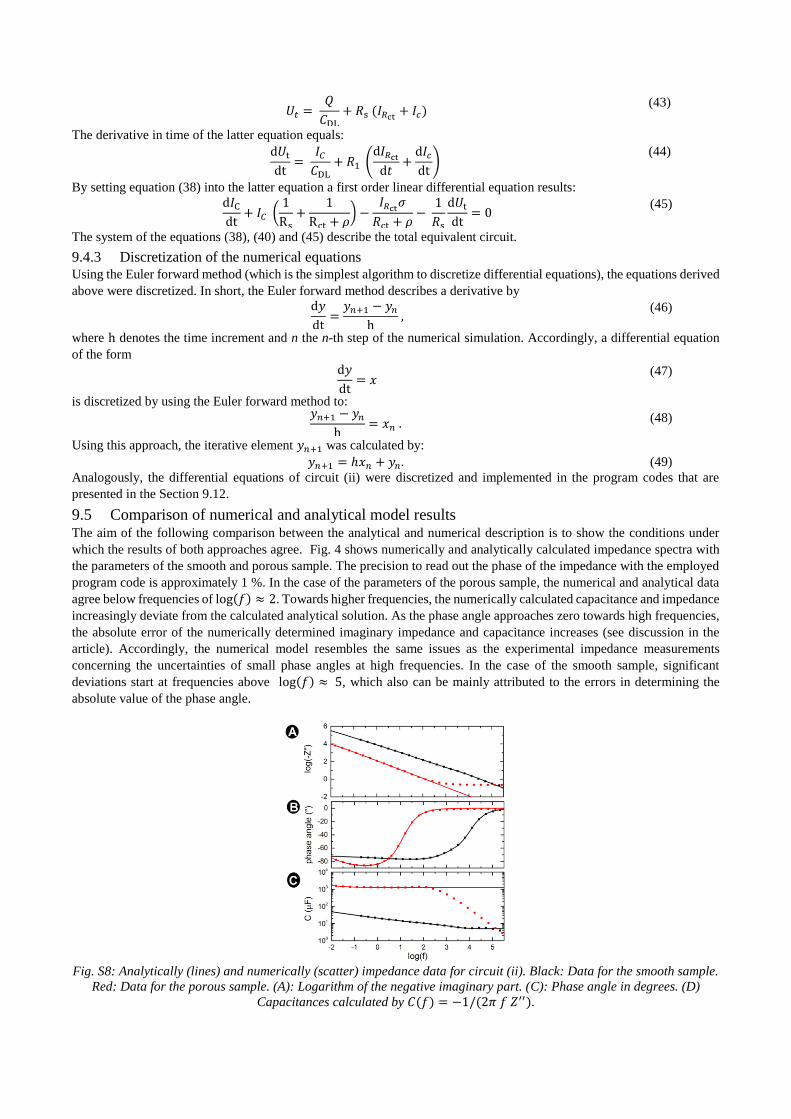
9.5 Comparison of numerical and analytical model results The aim of the following comparison between the analytical and numerical description is to show the conditions under

which the results of both approaches agree. Fig. 4 shows numerically and analytically calculated impedance spectra with

the parameters of the smooth and porous sample. The precision to read out the phase of the impedance with the employed

program code is approximately 1 %. In the case of the parameters of the porous sample, the numerical and analytical data

agree below frequencies of log(𝑓) ≈ 2. Towards higher frequencies, the numerically calculated capacitance and impedance

increasingly deviate from the calculated analytical solution. As the phase angle approaches zero towards high frequencies,

the absolute error of the numerically determined imaginary impedance and capacitance increases (see discussion in the

article). Accordingly, the numerical model resembles the same issues as the experimental impedance measurements

concerning the uncertainties of small phase angles at high frequencies. In the case of the smooth sample, significant

deviations start at frequencies above log(𝑓) ≈ 5, which also can be mainly attributed to the errors in determining the

absolute value of the phase angle.

Fig. S8: Analytically (lines) and numerically (scatter) impedance data for circuit (ii). Black: Data for the smooth sample.

Red: Data for the porous sample. (A): Logarithm of the negative imaginary part. (C): Phase angle in degrees. (D)

Capacitances calculated by 𝐶(𝑓) = −1/(2𝜋 𝑓 𝑍′′).

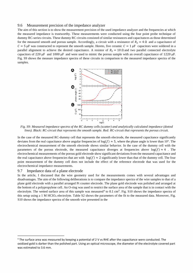
9.6 Measurement precision of the impedance analyzer The aim of this section is to show the measurement precision of the used impedance analyzer and the frequencies at which

the measured impedance is trustworthy. These measurements were conducted using the four point probe technique of

dummy RC-series circuits. These dummy RC circuits consisted of similar resistances and capacitances as those determined

for the measured smooth and porous sample. Accordingly, a circuit with a resistance of 𝑅𝑆 = 4 Ω and a capacitance of

𝐶 = 5 μF was constructed to represent the smooth sample. Hereto, five ceramic 𝐶 = 1 μF capacitors were soldered in a

parallel alignment to achieve the desired capacitance. A resistor of 𝑅𝑆 = 10 Ω and two parallel connected electrolyte

capacitors of 220 μF and 1000 μF and were used to mimic the porous sample with an overall capacitance of 1220 μF.

Fig. S9 shows the measure impedance spectra of these circuits in comparison to the measured impedance spectra of the

samples.

Fig. S9: Measured impedance spectra of the RC dummy cells (scatter) and analytically calculated impedance (dotted

lines). Black: RC-circuit that represents the smooth sample. Red: RC-circuit that represents the porous circuit.

In the case of the measured RC-dummy cell that represents the smooth electrode, the measured capacitance significantly

deviates from the real capacitance above angular frequencies of log(𝑓) ≈ 5, where the phase angle is lower than 10°. The

electrochemical measurement of the smooth electrode shows similar behavior. In the case of the dummy cell with the

parameters of the porous electrode, the measured capacitance diverges at frequencies above log(𝑓) ≈ 4 . The

electrochemical measurements of the porous gold electrode show significant deviations from the measured capacitance and

the real capacitance above frequencies that are with log(𝑓) ≈ 2 significantly lower than that of the dummy cell. The four

point measurement of the dummy cell does not include the effect of the reference electrode that was used for the

electrochemical impedance measurements.

9.7 Impedance data of a plane electrode In the article, I discussed that the wire geometry used for the measurements comes with several advantages and

disadvantages. The aim of the following deliberations is to compare the impedance spectra of the wire samples to that of a

plane gold electrode with a parallel arranged Pt counter electrode. The plane gold electrode was polished and arranged at

the bottom of a polypropylene cell. An O-ring was used to restrict the surface area of the sample that is in contact with the

electrolyte. The wetted surface area of this sample was measured4 to 0.1 cm². Fig. S10 shows the impedance spectra of

this setup using a 1 M HClO4 electrolyte. Table S2 shows the parameters of the fit to the measured data. Moreover, Fig.

S10 shows the impedance spectra of the smooth wire presented in the

4 The surface area was measured by keeping a potential of 2 V vs RHE after the capacitance were conducted. The oxidized gold is darker than the polished part. Using an optical microscope, the diameter of the electrolyte covered part was estimated to 3.6 mm.

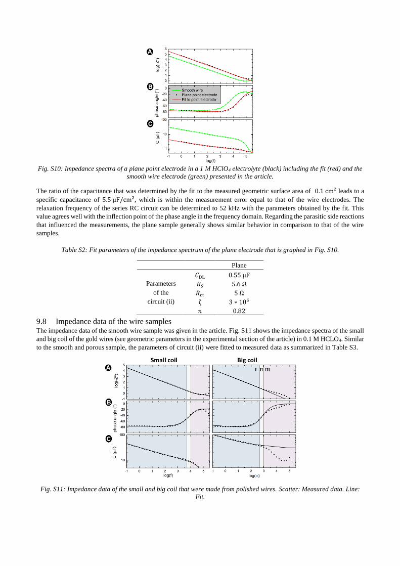
Fig. S10: Impedance spectra of a plane point electrode in a 1 M HClO4 electrolyte (black) including the fit (red) and the

smooth wire electrode (green) presented in the article.

The ratio of the capacitance that was determined by the fit to the measured geometric surface area of 0.1 cm² leads to a

specific capacitance of 5.5 μF/cm², which is within the measurement error equal to that of the wire electrodes. The

relaxation frequency of the series RC circuit can be determined to 52 kHz with the parameters obtained by the fit. This

value agrees well with the inflection point of the phase angle in the frequency domain. Regarding the parasitic side reactions

that influenced the measurements, the plane sample generally shows similar behavior in comparison to that of the wire

samples.

Table S2: Fit parameters of the impedance spectrum of the plane electrode that is graphed in Fig. S10.

Plane 𝐶DL 0.55 μF

Parameters 𝑅𝑆 5.6 Ω

of the 𝑅ct 5 Ω

circuit (ii) ζ 3 ∗ 105 𝑛 0.82

9.8 Impedance data of the wire samples The impedance data of the smooth wire sample was given in the article. Fig. S11 shows the impedance spectra of the small

and big coil of the gold wires (see geometric parameters in the experimental section of the article) in 0.1 M HCLO4. Similar

to the smooth and porous sample, the parameters of circuit (ii) were fitted to measured data as summarized in Table S3.

Fig. S11: Impedance data of the small and big coil that were made from polished wires. Scatter: Measured data. Line:

Fit.

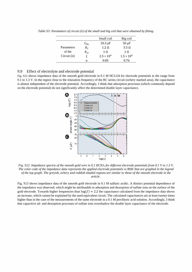
Table S3: Parameters of circuit (ii) of the small and big coil that were obtained by fitting.

Small coil Big coil 𝐶DL 10.3 μF 30 μF

Parameters 𝑅𝑆 1.2 Ω 5.5 Ω

of the 𝑅ct 1 Ω 1 Ω

Circuit (ii) ζ 2.5 ∗ 104 1.5 ∗ 104 𝑛 0.85 0.76

9.9 Effect of electrolyte and electrode potential Fig. S12 shows impedance data of the smooth gold electrode in 0.1 M HCLO4 for electrode potentials in the range from

0.1 to 1.3 V. In the region close to the relaxation frequency of the RC series circuit (ochery marked area), the capacitance

is almost independent of the electrode potential. Accordingly, I think that adsorption processes (which commonly depend

on the electrode potential) do not significantly affect the determined double layer capacitance.

Fig. S12: Impedance spectra of the smooth gold wire in 0.1 HClO4 for different electrode potentials from 0.1 V to 1.3 V.

The color code of the impedance data represents the applied electrode potentials vs RHE that are graphed in the legend

of the top graph. The greyish, ochery and reddish shaded regions are similar to those of the smooth electrode in the

article .

Fig. S13 shows impedance data of the smooth gold electrode in 0.1 M sulfuric acidic. A distinct potential dependence of

the impedance was observed, which might be attributable to adsorption and desorption of sulfate ions on the surface of the

gold electrode. Towards higher frequencies than log(𝑓) ≈ 2.2 the capacitance calculated from the impedance data shows

an increase, which cannot be explained by the used equivalent circuit. The calculated capacitances are at least twenty times

higher than in the case of the measurements of the same electrode in a 0.1 M perchloric acid solution. Accordingly, I think

that capacitive ad- and desorption processes of sulfate ions overshadow the double layer capacitance of the electrode.

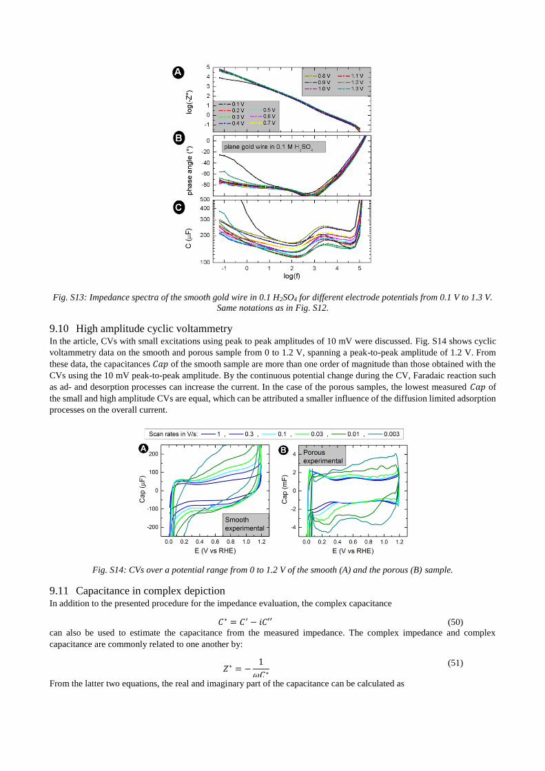
Fig. S13: Impedance spectra of the smooth gold wire in 0.1 H2SO4 for different electrode potentials from 0.1 V to 1.3 V.

Same notations as in Fig. S12.

9.10 High amplitude cyclic voltammetry In the article, CVs with small excitations using peak to peak amplitudes of 10 mV were discussed. Fig. S14 shows cyclic

voltammetry data on the smooth and porous sample from 0 to 1.2 V, spanning a peak-to-peak amplitude of 1.2 V. From

these data, the capacitances 𝐶𝑎𝑝 of the smooth sample are more than one order of magnitude than those obtained with the

CVs using the 10 mV peak-to-peak amplitude. By the continuous potential change during the CV, Faradaic reaction such

as ad- and desorption processes can increase the current. In the case of the porous samples, the lowest measured 𝐶𝑎𝑝 of

the small and high amplitude CVs are equal, which can be attributed a smaller influence of the diffusion limited adsorption

processes on the overall current.

Fig. S14: CVs over a potential range from 0 to 1.2 V of the smooth (A) and the porous (B) sample.

9.11 Capacitance in complex depiction In addition to the presented procedure for the impedance evaluation, the complex capacitance

𝐶∗ = 𝐶′ − 𝑖𝐶′′ (50)

can also be used to estimate the capacitance from the measured impedance. The complex impedance and complex

capacitance are commonly related to one another by:

𝑍∗ = −1

𝜔𝐶∗

(51)

From the latter two equations, the real and imaginary part of the capacitance can be calculated as

𝐶′ = −𝑍′′

𝜔 |𝑍|2

(52)

and

𝐶′′ = −𝑍′

𝜔 |𝑍|2

(53)

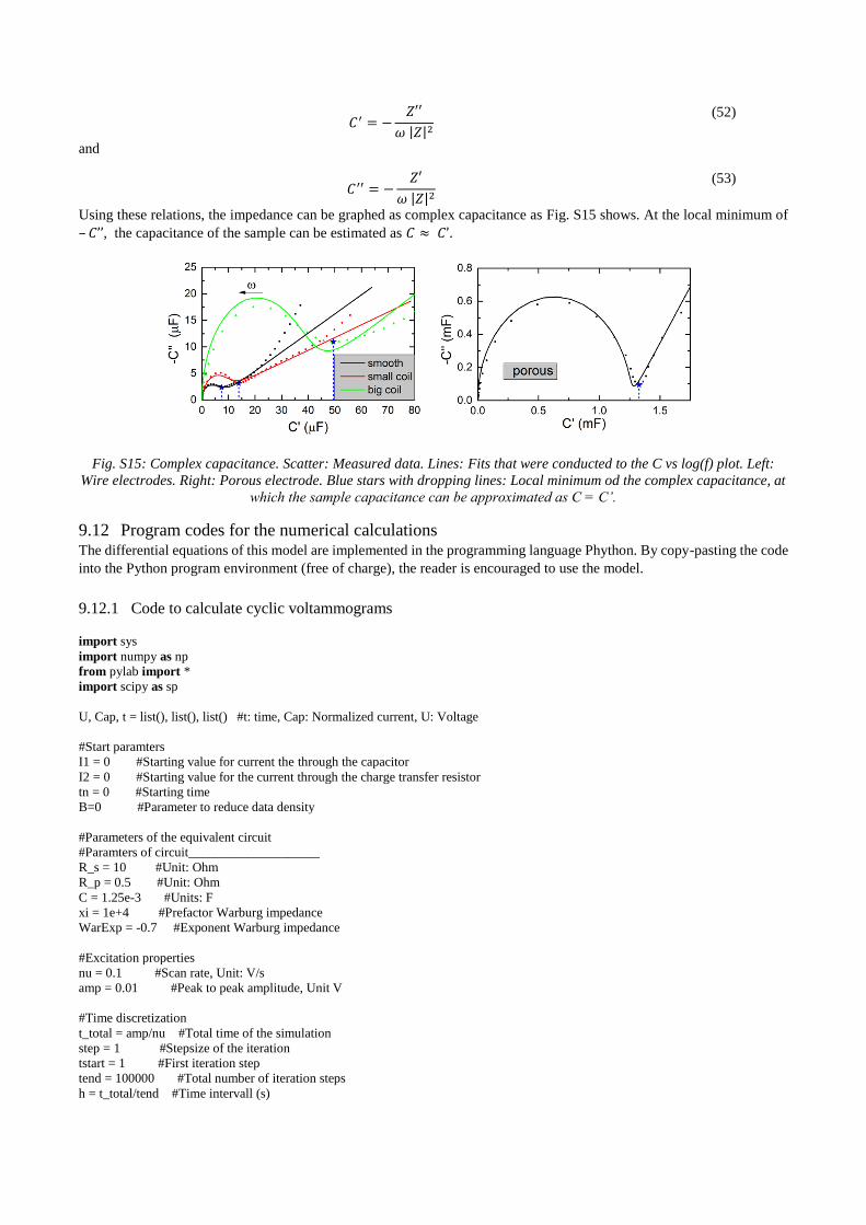
Using these relations, the impedance can be graphed as complex capacitance as Fig. S15 shows. At the local minimum of

– 𝐶’’, the capacitance of the sample can be estimated as 𝐶 ≈ 𝐶’.

Fig. S15: Complex capacitance. Scatter: Measured data. Lines: Fits that were conducted to the C vs log(f) plot. Left:

Wire electrodes. Right: Porous electrode. Blue stars with dropping lines: Local minimum od the complex capacitance, at

which the sample capacitance can be approximated as C = C’.

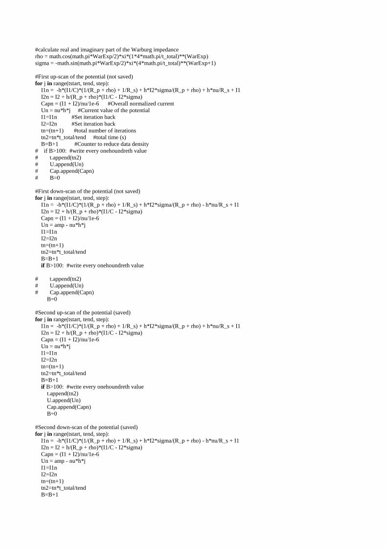
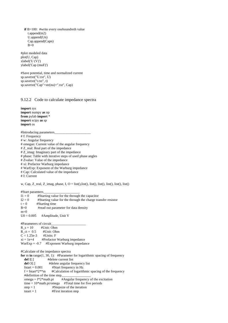
9.12 Program codes for the numerical calculations The differential equations of this model are implemented in the programming language Phython. By copy-pasting the code

into the Python program environment (free of charge), the reader is encouraged to use the model.

9.12.1 Code to calculate cyclic voltammograms

import sys

import numpy as np

from pylab import *

import scipy as sp

U, Cap, t = list(), list(), list() #t: time, Cap: Normalized current, U: Voltage

#Start paramters

I1 = 0 #Starting value for current the through the capacitor

I2 = 0 #Starting value for the current through the charge transfer resistor

tn = 0 #Starting time

B=0 #Parameter to reduce data density

#Parameters of the equivalent circuit

#Paramters of circuit____________________

R_s = 10 #Unit: Ohm

R_p = 0.5 #Unit: Ohm

C = 1.25e-3 #Units: F

xi = 1e+4 #Prefactor Warburg impedance

WarExp = -0.7 #Exponent Warburg impedance

#Excitation properties

nu = 0.1 #Scan rate, Unit: V/s

amp = 0.01 #Peak to peak amplitude, Unit V

#Time discretization

t_total = amp/nu #Total time of the simulation

step = 1 #Stepsize of the iteration

tstart = 1 #First iteration step

tend = 100000 #Total number of iteration steps

h = t_total/tend #Time intervall (s)

#calculate real and imaginary part of the Warburg impedance

rho = math.cos(math.pi*WarExp/2)*xi*(1*4*math.pi/t_total)**(WarExp)

sigma = -math.sin(math.pi*WarExp/2)*xi*(4*math.pi/t_total)**(WarExp+1)

#First up-scan of the potential (not saved)

for j in range(tstart, tend, step):

I1n = -h*(I1/C)*(1/(R_p + rho) + 1/R_s) + h*I2*sigma/(R_p + rho) + h*nu/R_s + I1

I2n = I2 + h/(R_p + rho)*(I1/C - I2*sigma)

Capn = (I1 + I2)/nu/1e-6 #Overall normalized current

Un = nu*h*j #Current value of the potential

I1=I1n #Set iteration back

I2=I2n #Set iteration back

tn=(tn+1) #total number of iterations

tn2=tn*t_total/tend #total time (s)

B=B+1 #Counter to reduce data density

# if B>100: #write every onehoundreth value

# t.append(tn2)

# U.append(Un)

# Cap.append(Capn)

# B=0

#First down-scan of the potential (not saved)

for j in range(tstart, tend, step):

I1n = -h*(I1/C)*(1/(R_p + rho) + 1/R_s) + h*I2*sigma/(R_p + rho) - h*nu/R_s + I1

I2n = I2 + h/(R_p + rho)*(I1/C - I2*sigma)

Capn = (I1 + I2)/nu/1e-6

Un = amp - nu*h*j

I1=I1n

I2=I2n

tn=(tn+1)

tn2=tn*t_total/tend

B=B+1

if B>100: #write every onehoundreth value

# t.append(tn2)

# U.append(Un)

# Cap.append(Capn)

B=0

#Second up-scan of the potential (saved)

for j in range(tstart, tend, step):

I1n = -h*(I1/C)*(1/(R_p + rho) + 1/R_s) + h*I2*sigma/(R_p + rho) + h*nu/R_s + I1

I2n = I2 + h/(R_p + rho)*(I1/C - I2*sigma)

Capn = (I1 + I2)/nu/1e-6

Un = nu*h*j

I1=I1n

I2=I2n

tn=(tn+1)

tn2=tn*t_total/tend

B=B+1

if B>100: #write every onehoundreth value

t.append(tn2)

U.append(Un)

Cap.append(Capn)

B=0

#Second down-scan of the potential (saved)

for j in range(tstart, tend, step):

I1n = -h*(I1/C)*(1/(R_p + rho) + 1/R_s) + h*I2*sigma/(R_p + rho) - h*nu/R_s + I1

I2n = I2 + h/(R_p + rho)*(I1/C - I2*sigma)

Capn = (I1 + I2)/nu/1e-6

Un = amp - nu*h*j

I1=I1n

I2=I2n

tn=(tn+1)

tn2=tn*t_total/tend

B=B+1

if B>100: #write every onehoundreth value

t.append(tn2)

U.append(Un)

Cap.append(Capn)

B=0

#plot modeled data

plot(U, Cap)

xlabel('U (V)')

ylabel('Cap (muF)')

#Save potential, time and normalized current

sp.savetxt("U.txt", U)

sp.savetxt("t.txt", t)

sp.savetxt("Cap"+str(nu)+".txt", Cap)

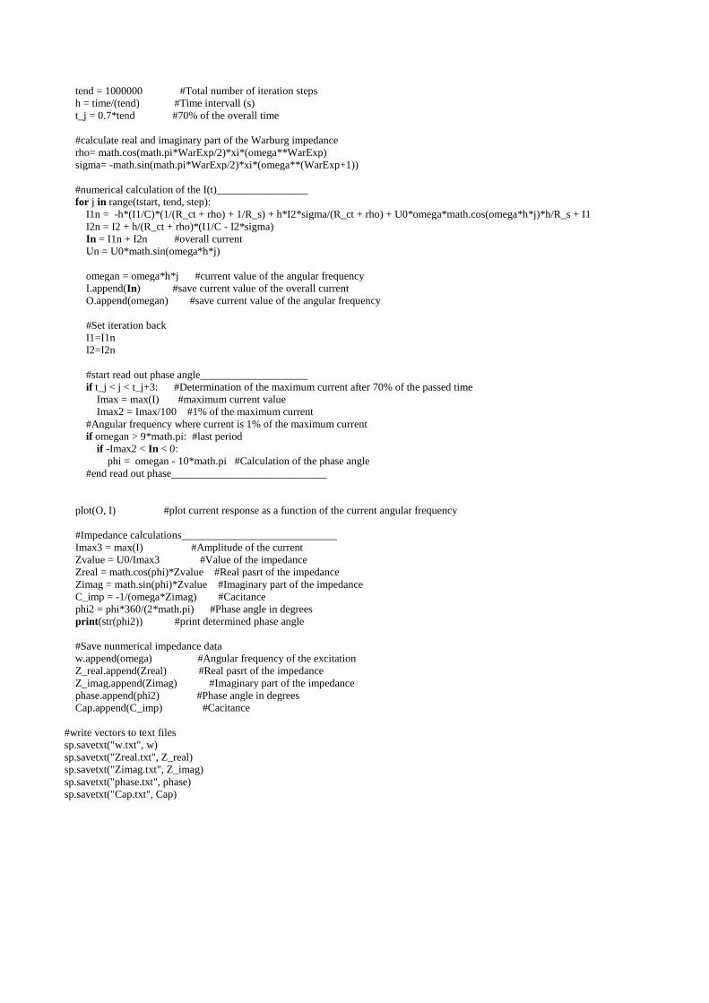
9.12.2 Code to calculate impedance spectra

import sys

import numpy as np

from pylab import *

import scipy as sp

import os

#Introducing parameters_____________________

# f: Frequency

# w: Angular frequency

# omegan: Current value of the angular frequency

# Z_real: Real part of the impedance

# Z_imag: Imaginary part of the impedance

# phase: Table with iterative steps of used phase angles

# Zvalue: Value of the impedance

# xi: Prefactor Warburg impedance

# WarExp: Exponent of the Warburg impedance

# Cap: Calculated value of the impedance

# I: Current

w, Cap, Z_real, Z_imag, phase, I, O = list(),list(), list(), list(), list(), list(), list()

#Start paramters_____________________

I1 = 0 #Starting value for the through the capacitor

I2 = 0 #Starting value for the through the charge transfer resistor

t = 0 #Starting time

B=0 #read out parameter for data density

m=0

U0 = 0.005 #Amplitude, Unit V

#Parameters of circuit____________________

R_s = 10 #Unit: Ohm

R_ct = 0.5 #Unit: Ohm

C = 1.25e-3 #Units: F

xi = 1e+4 #Prefactor Warburg impedance

WarExp = -0.7 #Exponent Warburg impedance

#Calculate of the impedance spectra

for m in range(1, 30, 1): #Parameter for logarithmic spacing of frequency

del I[:] #delete current list

del O[:] #delete angular frequency list

fstart = 0.001 #Start frequency in Hz

f = fstart*2**m #Calculation of logarithmic spacing of the frequency

#definition of the time step_________________

omega = f*2*math.pi #Angular frequency of the excitation

time = 10*math.pi/omega #Total time for five periods

step = 1 #Stepsize of the iteration

tstart = 1 #First iteration step

tend = 1000000 #Total number of iteration steps

h = time/(tend) #Time intervall (s)

t_j = 0.7*tend #70% of the overall time

#calculate real and imaginary part of the Warburg impedance

rho= math.cos(math.pi*WarExp/2)*xi*(omega**WarExp)

sigma= -math.sin(math.pi*WarExp/2)*xi*(omega**(WarExp+1))

#numerical calculation of the I(t)_________________

for j in range(tstart, tend, step):

I1n = -h*(I1/C)*(1/(R_ct + rho) + 1/R_s) + h*I2*sigma/(R_ct + rho) + U0*omega*math.cos(omega*h*j)*h/R_s + I1

I2n = I2 + h/(R_ct + rho)*(I1/C - I2*sigma)

In = I1n + I2n #overall current

Un = U0*math.sin(omega*h*j)

omegan = omega*h*j #current value of the angular frequency

I.append(In) #save current value of the overall current

O.append(omegan) #save current value of the angular frequency

#Set iteration back

I1=I1n

I2=I2n

#start read out phase angle____________________

if t_j < j < t_j+3: #Determination of the maximum current after 70% of the passed time

Imax = max(I) #maximum current value

Imax2 = Imax/100 #1% of the maximum current

#Angular frequency where current is 1% of the maximum current

if omegan > 9*math.pi: #last period

if -Imax2 < In < 0:

phi = omegan - 10*math.pi #Calculation of the phase angle

#end read out phase_____________________________

plot(O, I) #plot current response as a function of the current angular frequency

#Impedance calculations_____________________________

Imax3 = max(I) #Amplitude of the current

Zvalue = U0/Imax3 #Value of the impedance

Zreal = math.cos(phi)*Zvalue #Real pasrt of the impedance

Zimag = math.sin(phi)*Zvalue #Imaginary part of the impedance

C_imp = -1/(omega*Zimag) #Cacitance

phi2 = phi*360/(2*math.pi) #Phase angle in degrees

print(str(phi2)) #print determined phase angle

#Save nunmerical impedance data

w.append(omega) #Angular frequency of the excitation

Z_real.append(Zreal) #Real pasrt of the impedance

Z_imag.append(Zimag) #Imaginary part of the impedance

phase.append(phi2) #Phase angle in degrees

Cap.append(C_imp) #Cacitance

#write vectors to text files

sp.savetxt("w.txt", w)

sp.savetxt("Zreal.txt", Z_real)

sp.savetxt("Zimag.txt", Z_imag)

sp.savetxt("phase.txt", phase)

sp.savetxt("Cap.txt", Cap)