Impartial Trimmed Means for Functional Data

Impartial Trimmed Means for Functional Data

Juan Antonio Cuesta-Albertos and Ricardo Fraiman

Abstract. In this paper we extend the notion of impartial trimming to afunctional data framework, and we obtain resistant estimates of the centerof a functional distribution. We give mild conditions for the existence anduniqueness of the functional trimmed means. We show the continuity of thepopulation parameter with respect to the weak convergence of probabilitymeasures. As a consequence we obtain consistency and qualitative resistanceof the data based estimates. A simplified approximate computational methodis also given. Some real data examples are finally analyzed.

1. Introduction

Real time monitoring of many processes are available for applications and mod-eling in different fields such as medicine, neuroscience, chemometrics, signal trans-mission, stock markets, meteorology and TV audience ratings. In this context theindividual observed responses are rather curves than finite dimensional vectors, andmay be modeled as sampling paths X(t, ω), ω ∈ Ω, of independent realizations ofa stochastic process centered at a function µ(t), i.e., functional data.

In practice, the use of functional data is often preferable to that of large finitedimensional vectors obtained by discrete approximations of the functions (see forinstance the books by Ramsay and Silverman [38, 39]). In [13, 36, 1, 24, 10, 4,20, 37, 40, 26, 25, 6, 15, 16, 30, 2, 19, 12], and the references therein, we haveseveral case–studies and/or theoretical developments for functional data.

Robustness has been an almost not explored area in this context of functionaldata, never the less there is no reason why we should not expect the presenceof outliers in there. For one dimensional data, the simplest robust estimates ofa location parameter are the well known trimmed-mean estimates, a family thatgoes from the sample mean to the sample median as increasing the trimming level.However, there is not a standard way to extend it to higher dimensions. Theconcept of trimmed-means and medians has been a topic of active research in thelast decade, even for two dimensional data.

Usually, trimming is associated to ranks, but in more than one dimension, theconcepts of order statistics and ranks are more involved and several definitions have

1991 Mathematics Subject Classification. Primary 62H30, 62F15, 62G07; Secondary 62F35.Key words and phrases. Impartial trimming, robustness, mean, functional data, consistency,

uniqueness.The first author was supported in part by the Spanish Ministerio de Ciencia y Tecnologıa,

grant BFM2002-04430-C02-02.

1

2 JUAN ANTONIO CUESTA-ALBERTOS AND RICARDO FRAIMAN

been proposed for the finite dimensional case. See, for instance, [31, 43, 5, 34,27, 28, 41, 22, 42, 14, 29, 18] and the book by Mosler [33]. All of them arebased on different notions of depth concepts, a device introduced to measure thecentrality of a vector within a given data cloud.

A different approach to trimming, which is not based on ranks, is the “impar-tial trimming” (self–determined by the data) which was introduced by Gordalizain [22] for the multivariate location model and will be described in detail later on.Roughly speaking, impartial–trimming means that the trimming is not necessar-ily symmetric, and the data which are to be trimmed are self–determined by theestimate based on the whole data cloud. Moreover, even in the one-dimensionalcase, has the main advantage over the usual trimming that it is not required tofix a special zone or direction in advance in which the data will be trimmed. Thisproperty has shown to be important when dealing with asymmetric contamination.

For a related problem, Cuesta–Albertos, Gordaliza and Matran [8, 9] intro-duced a class of procedures based on “impartial trimming” to robustify k-meansfor clustering methods in the finite dimensional case. See also [32, 11].

We will employ this approach to define trimmed means for functional data, andstudy their asymptotic properties under mild conditions.

A robust estimate of the center of a functional distribution has been proposed byFraiman and Muniz in [19]. They define trimmed means for functional data basedon a functional depth concept, which is defined as an integral of the univariatedepths at each single point t. It is useful to point here that two main differenceswith the present work, besides the different approach to the problem, can be stated:

(a) the approach introduced here can be extended to the case of trimmedk-means in a similar way as in [8, 9] where they generalize the work [22].

(b) here the results are obtained under mild assumptions on the underlyingstochastic process. This is not the case in [19] where strong regularityconditions are required on the trajectories of the process.

From here on we proceed as follow. In Section 2 we borrow the definitionof qualitative robustness given in [3] and adapt it to the case of functional dataconsidering a new distance between trajectories. In Section 3 we define a robustestimate based on the concept of impartial trimming. We show the existence of anoptimal trimming, and, based on this optimal trimming, we define our estimate.We prove the strong consistency and robustness of the estimate.

In Section 4 we give conditions for the uniqueness of the parameter to be esti-mated. We introduce the concept of symmetric unimodality for stochastic processeswhich turns out to be a sufficient condition for the uniqueness of the impartialtrimmed–mean parameter. The interest of the uniqueness of the target parameterrelies on the fact that uniqueness is required in order to obtain robustness. (Thisis also the case for one dimensional distributions. For instance, the median is notqualitative robust if the underlying distribution of the random variable X satis-fies P [X = −1] = P [X = 1] = 0.5.) Sharp conditions for the uniqueness of theimpartial trimmed mean parameter, even in a finite dimensional setup, remainsstill an open problem. In this Section we provide an example of a symmetrical,strictly unimodal two-dimensional distribution with strictly positive differentiabledensity function for which not only the uniqueness fails but the parameter is notthe symmetry center. Moreover, at this time we are only aware of the existence oftwo uniqueness results. The first one, in [22], is for one dimensional distributions

IMPARTIAL TRIMMED MEANS FOR FUNCTIONAL DATA 3

and requires that the distribution be unimodal, with a differentiable and strictlypositive density function. The second one, in [21], applies to elliptical, unimodal,differentiable and strictly positive densities.

Computational problems are studied in Section 5 where we introduce a sim-pler consistent alternative estimate, which can be also used as a starting point foran algorithm searching for the proposed estimate. In Section 6 we analyze somereal data examples from TV ratings. Most of the proofs and technical results aredeferred to the Appendix.

In what follows we restrict to consider L2[0, 1]-valued random elements. How-ever, most of the present results can be extended in a straightforward way to thecase of random elements (r.e.’s) with values in an uniformly convex Banach space.

2. Qualitative Robustness

Hampel, in [23], introduced the concept of qualitative robustness for a sequenceof estimates of a finite dimensional parameter in the case of independent and iden-tically distributed (i.i.d.) observations. His definition stated that a sequence ofestimates Tn is robust at a given distribution µ if for any other distribution µ closeto µ in the Prohorov metric, the distribution of Tn under µ and under µ are closein the Prohorov metric, uniformly in the sample size.

The use of the Prohorov distance reflects the intuitive meaning of robustness asinsensitivity of the estimate to round-off errors, and to a small fraction of outliers.

Boente, Fraiman and Yohai in [3] extended these notions to the case of sto-chastic processes with dependent variables, and introduced a new definition of ro-bustness based on the concept of resistance (see also [35, 7]). In a functional datasetup robustness should reflect insensitivity of the estimate to two kinds of differentcontamination. Firstly, following Hampel, the notion of robustness should take careof:

(a) small errors in all the realizations of the process (e.g. round-off errors).(b) a small fraction of far away curves (outliers).

However, it may also happen that in a functional data framework, a muchwilder kind of contamination be present: each curve can be “out of control” duringa small fraction of time. Thus, the second notion of robustness should also takeinto consideration that:

(c) each curve may be disturbed in a small time interval.

This last type of contamination is much wilder than the first one, since it allows,in principle, all the data to be contaminated, each curve at a different small intervalof time. If the data have sharp peaks at different intervals a robust procedure shouldmainly ignore (or, in some way, delete) those peaks. However, if we have some kindof data such that, most of it, presents a sharp spike in the same interval, then themethod should not delete it. This effect can be seen in the following example.

In [17] the behavior of electric power consumers at Buenos Aires, Argentina,is analyzed. For every individual (household) in the sample, measurements weretaken at each of the 96 intervals of 15 minutes in every weekday (Monday to Friday)during January 2001. Monthly averages over days for each individual were analyzed.The main conclusion, was that with respect to the peaks, two typical consumer’sbehavior were found. One with only a peak around 9:00 pm, while another group


Figure 1. Electrical power typical consumers at Buenos Aires,Argentina. Curves represent the mean along week days in January2001 of instantaneous consume, measured every 15 minutes alongthe day. Right: Three typical members of the group with only apeak at night. Left: Three typical members of the group with asecond peak around noon.

had also a peak around noon. In Figure 1 we plot the curves corresponding to someof the typical consumers in each group.

In this work, the important feature of the data was precisely the hours atwhich maximum consume was attained. On the other hand, if we use a naiverobust estimate that starts by a simple “cut-off” of sharp peaks, we could loose thischaracteristic.

In this paper, we propose here an estimate which is able to handle the moreclassical contamination models that takes care of (a) and (b). Another type ofestimates are necessary to deal with contamination of type (c). At this time wehave some idea on how to handle this contamination and it is the subject of someresearch in progress.

To finalize this section, we present some definitions which should be fulfilled byestimates robust against those kind of contaminations. Let E = L2[0, 1], and, forx, y ∈ L2[0, 1] we will denote,

d(x, y) = ‖x− y‖ =(∫ 1

0

|x(t)− y(t)|2dt

)1/2

.

In order to define robustness we borrow the ideas in [3]. First, we introduce ametric dn and a pseudo-metric dn,c, that will be used for the two different robustnessdefinitions. Let xn := (x1, x2, ..., xn) and yn := (y1, y2, ..., yn) with xi, yi ∈ E, i ≥ 1,and define

dn(xn, yn) = infε : (#i : d(xi, yi) ≥ ε)/n ≤ ε,


where #A denotes the cardinal of the set A. If each yi, i = 1, ..., n is obtainedcontaminating the corresponding xi, i = 1, ..., n with contamination of type (a) or(b), this definition makes xn and yn be close.

On the other hand, if we define

dn,c(xn, yn) = infε : (#i : dc,ε(xi, yi) ≥ ε)/n ≤ ε

with

dc,ε(xi, yi) = infA⊂[0,1]

(∫[0,1]−A

|xi(t)− yi(t)|2dt

)1/2

, i = 1, ..., n,

where λ(A) < ε and λ(.) stands for the Lebesgue measure, we obtain a distancewhich makes xnand yn to be close also under contamination of type (c).

Let (F,D) be a metric space and Tn : En → F be a sequence of estimatestaking values in F . Let x = (xn : n ≥ 1) ∈ E∞, and Πn(x) = (x1, x2, ..., xn) ∈ En

be the canonical projection on the first n coordinates. Define

∆n(δ,Πn(x)) = supD[Tn(yn), Tn(Πn(x))] : yn ∈ B(Πn(x), δ, dn),

where B(Πn(x), δ, dn) stands for the open ball in En centered at Πn(x) and radiusδ with respect to the metric dn.

Definition 2.1. Let x ∈ E∞. Tn is resistant at x if, given ε > 0, there existδ > 0, n0 ∈ IN such that ∆n(δ,Πn(x)) ≤ ε, fore very n ≥ n0.

Definition 2.2. Tn is robust at µ, where µ is a probability measure on E∞, if

µ (x ∈ E∞ : Tn is resistant at x) = 1.

Changing dn by dn,c in the previous definitions we get a notion of robustness,that also deals with (c)–type contamination.

3. Definition and properties.

In this paper we will be concerned only with L2[0, 1]-valued r.e.’s which, unlessotherwise stated, will be defined on the same rich enough probability space (Ω, σ, µ).P will be a fixed probability distribution on the Borel σ algebra on E.

Our robust estimate is based on the idea of impartial trimming introduced in[22] which can be extended to the infinite dimensional case in the following way.

Let α ∈ (0, 1). We will say that a measurable function τ : E → [0, 1] is a trimat level α for P if ∫

τ(y)dP (y) ≥ 1− α.

The function τ tells us which part of every point must be trimmed taking intoaccount that a maximum trim of α is allowed.

Let us denote by Pα the family of all trims at level α for P .We divide this section in three subsections. In the first one we prove the exis-

tence of an optimal trimming in the sense of (3.1) below. In the second one we provethe continuity of the trimmed mean population parameter (see definition below)with respect to the convergence in distribution. In the third one, we introduce theestimate and, as a consequence of the results in previous subsection, we obtain thestrong consistency and qualitative robustness of the sequence of empirical trimmedmean estimates.


3.1. Definition of population parameter and existence of an optimaltrimming. Given α ∈ (0, 1), we will show that there exist a point mP ∈ E andτP ∈ Pα, which are optimal in the following sense

(3.1) Iα(P ) := infm∈E,τ∈Pα

∫||y −m||2τ(y)dP (y) =

∫||y −mP ||2τP (y)dP (y).

We will call α-trimmed mean or, simply, trimmed mean, to every mP such thatthere exists a trimming function τP ∈ Pα which satisfy (3.1). τP will be calledoptimal trimming function. If we apply equation (3.1) to the empirical probabilitymeasure Pn, we obtain the empirical α-trimmed mean estimate.

It is possible to extend the previous definition to obtain (Φ, α)-trimmed means(and estimates), as in [22], introducing a continuous and non decreasing weightfunction Φ such that

limt→∞

Φ(t) > Φ(x) for every x ∈ R+,

replacing equation (3.1) by

Iα,Φ(P ) := infm∈E,τ∈Pα

∫Φ [||y −m||] τ(y)dP (y) =

∫Φ [||y −mP ||] τP (y)dP (y).

This family extends the so-called Z-estimates (see, for instance, [44]). However,for the sake of notation, we will assume throughout that Φ(t) = t2.

We start with some previous results. The following lemma states a very wellknown property of the mean and justifies the name of trimmed mean we have givento mP .

Lemma 3.1. Let α > 0 and let τ ∈ Pα. If we define

xτ :=∫

yτ(y)dP (y)∫τ(y)dP (y)

,

then ∫||y − xτ ||2τ(y)dP (y) ≤

∫||y − x||2τ(y)dP (y), for every x ∈ E.

We introduce now some additional notation. Given m ∈ E and r > 0, letB(m, r) (resp. B(m, r)) denotes the open (resp. closed) ball centered at m withradius r. S(m, r) will stand for the associated sphere. Let us also define

rα(m) := infr > 0 : P [B(m, r)] ≥ 1− α.

It follows that if r < rα(m) then P [B(m, r)] < 1− α and

P [B(m, rα(m))] ≤ 1− α ≤ P [B(m, rα(m))].

Proposition 3.2. Let α > 0, m ∈ E and let τm ∈ Pα be such that

(3.2)∫

τm(y)dP (y) = 1− α and IB(m,rα(m)) ≤ τm ≤ IB(m,rα(m)).

Then, we have that for every τ ∈ Pα,

(3.3)∫||y −m||2τm(y)dP (y) ≤

∫||y −m||2τ(y)dP (y).


Proof. Let τ ∈ Pα. We have that∫||y −m||2τ(y)dP (y)−

∫||y −m||2τm(y)dP (y)

=∫

B(m,rα(m))

||y −m||2(τ(y)− 1)dP (y) +∫

Bc(m,rα(m))

||y −m||2τ(y)dP (y)

+∫

S(m,rα(m))

||y −m||2(τ(y)− τm(y))dP (y)

≥ r2α(m)

(∫B(m,rα(m))

(τ(y)− 1)dP (y) +∫

Bc(m,rα(m))

τ(y)dP (y)

+∫

S(m,rα(m))

(τ(y)− τm(y))dP (y)

)≥ 0,

where the first inequality follows from the fact that τ ∈ [0, 1] and the second onefrom the definition of Pα and (3.2).

From equation (3.3), if we denote

(3.4) Dα(m,P ) :=∫||y −m||2τm(y)dP (y),

we obtain easily the following corollary.

Corollary 3.3. Let α > 0 and let P be a probability measure. Then, mP ∈ Eis a trimmed mean parameter of P if and only if

Dα(mP , P ) ≤ Dα(m,P ), for every m ∈ E.

Remark 3.4. Equality in (3.3) is only possible if τ satisfies (3.2). Therefore,according to Proposition 3.2, if an optimal trimming function, τP , does exist, itssupport is a ball with center at the trimmed mean mP . Its radius is rα(mP ). If thetrimmed mean is unique, we will often denote it rα(P ) and we will call it trimmingradius. In what follows, in order to simplify the notation, we will often suppressthe symbol α in the subindices, since it is fixed.

Remark 3.5. If we fix m, the value∫||y −m||2τ(y)dP (y)

does not depend on τ as long as τ satisfies (3.2). This justify the notation introducedin (3.4) and allows us to represent by τm to every trim at level α for P which satisfies(3.2).

Now we are able to establish the existence result. The proof is given in theAppendix.

Theorem 3.6. (Existence of optimal trimming) Let α ∈ (0, 1) and let P be aprobability measure on E. Then there exists mP ∈ E such that

Iα(P ) = Dα(mP , P ).

Obviously, uniqueness of of mP is not guaranteed by this result.


3.2. Continuity. In order to prove consistency and qualitative robustness,we will show the continuity of the trimmed mean parameter with respect to theconvergence in distribution. The proof relies in a technique introduced in [10], andis given in the Appendix.

Theorem 3.7. (Continuity) Let Pn be a sequence of probability measureswhich converges in distribution to the probability measure P . Let α ∈ (0, 1) and letus assume that the trimmed mean of P is unique.

Let mn be a sequence of trimmed means of Pn and denote by rn thesequence of the associated trimming radius. Then

lim ||mn −mP || = 0 and lim rn = r(P ).

Remark 3.8. Without the uniqueness assumption in Theorem 3.7, it can bestill proved, with the same proof, that the sequence mn is sequentially compactin norm and that every accumulation point is an α-trimmed mean of P .

From this remark and Theorem 3.7 we can obtain the following corollary. Itsproof (which is deferred to the Appendix) does not require the uniqueness assump-tion.

Corollary 3.9. Let Pn be a sequence of probability measures which con-verges in distribution to the probability measure P . If α ∈ (0, 1), then

lim Iα(Pn) = Iα(P ).

3.3. Estimates. Consistency and robustness. Let Xn be a sequence ofi.i.d. r.e.’s with distribution P . For every n ∈ IN , we will consider the empiricalprobability measure Pn defined by

Pn :=1n

∑i≤n

δXi(ω), ω ∈ Ω,

where δx denotes for Dirac’s delta measure on x.Given α ∈ (0, 1), we will denote by mω

n any empirical trimmed mean and by τωn

the associated empirical trimming function. The radius of the empirical trimmingfunction will be denote by rω

n .We estimate mP by the sequence mω

n and r(P ) by rωn. The consistency

result is the following.

Theorem 3.10. (Strong Consistency) Let α ∈ (0, 1) and let us assume thatthe probability P has a unique trimmed mean parameter. Let Xn be a sequenceof i.i.d. r.e.’s with distribution P . Then, every sequence of the empirical trimmedmeans and empirical trimming radius satisfy that

lim ||mωn −mP || = 0 and lim rω

n = r(P ), for µ-a.e. ω ∈ Ω.

Proof. This result is, in fact, a corollary of the extension to Banach spaces ofGlivenko-Cantelli’s Theorem and Theorem 3.7.

The resistance of our procedure can be deduced from the results in [3] although,we include an independent proof in the Appendix.


Theorem 3.11. (Robustness) Let us assume that the probability P satisfiesthat its trimmed mean is unique. Let Xn be a sequence of i.i.d. r.e.’s withdistribution P . Then any sequence of empirical trimming means is robust at P∞.

4. Uniqueness of the trimmed mean parameter. Unimodality

In this section we will give a sufficient condition (given in (4.1) below) forthe uniqueness of the trimmed mean parameter of a distribution. In the finitedimensional case it is closely related to symmetry and unimodality.

Definition 4.1. Let X be an E-valued r.e. We will say that its distributionis symmetrical and unimodal with mode at m0 if the distribution of X satisfies

(4.1) P [B(m0, r)] > P [B(m, r)], for every m ∈ E and r > 0.

In the one dimensional case, it is easy to see that if X is symmetrical around mand unimodal, then (4.1) holds; moreover, if P satisfies (4.1), then it can be shownthat P is continuous, symmetrical around m0 and has a unique mode at m0 in thesense that, for every m > m0 and δ > 0 it follows that

P [m,m + δ] > P [m + δ,m + 2δ].

On the other hand, condition (4.1) holds for every finite-dimensional distribu-tion which admits a representation similar to the one given in Theorem 4.4 below.However, we want to remark that unimodality plus symmetry are not enough toguarantee the uniqueness of the trimmed mean as shown in the following example.

Example 4.2. Let us consider the two dimensional and bounded set

A := B(0, 100)⋂[(

[−10, 10]× [−1, 1])⋃

(x1, x2) : |x1| ≤ 10|x2|]

,

where 0 = (0, 0). Let PA be the uniform distribution on A, m0 = (20, 0) and let usassume we want to compute the α-trimmed mean of PA with α = 1−PA[B(m0, 5)].Obviously

(4.2) Dα(0, PA) > Dα(m0, PA).

Given λ > 0, let Pλ be the probability distribution supported on A with densityfunction given by

fλ(x) := K[1 + λ(100− ||x||)IA(x)],where the constant K is chosen in order that fλ be a density function. Therefore,the level curves of Pλ are the intersection of spheres with A, and the parameter λdescribes how step is fλ. Moreover, fλ is strictly unimodal, for every x ∈ IR2:

fλ(x) = fλ(−x)

and the function t :→ fλ(tx), t ∈ IR, is strictly decreasing on t > 0 : tx ∈ A. Wealso have that

limλ→0+

Pλ = PA and limλ→0+

Dα(z, Pλ) = Dα(z, PA), z = 0,m0.

Thus, by (4.2) there exists λ0 such that Dα(0, Pλ0) > Dα(m0, Pλ0) and 0 is notthe trimmed mean of Pλ0 and, by the symmetry of this distribution, the trimmedmean is not unique.

Notice that a slight modification of this example allows to choose Pλ0 supportedby IR2 and fλ0 satisfying any desired regularity condition.


Theorem 4.3. Let P be a probability measure such that there exists m0 ∈ Ewhich satisfies (4.1).

Then, for every α ∈ (0, 1), the trimmed mean of P is unique and coincides withm0.

Proof. Let α > 0. Given m ∈ E and τm a trim at level α for P which satisfies(3.2), the function

r → Qm(r) :=1

1− α

∫B(m,r)

τm(y)dP (y), r ≥ 0,

is a distribution function and satisfies that

Dα(m,P ) = (1− α)∫

r2dQm(r).

Moreover, (4.1) implies that the distribution Qm0 is strictly stochasticallysmaller than Qm and, in consequence,

Dα(m0, P ) < Dα(m,P ).

The next theorem and corollary state that the class of symmetrical and uni-modal distributions is rich enough in the infinite dimensional case. The proof isgiven in the Appendix

Theorem 4.4. Let e1, e2, ... be a fixed orthonormal basis of E. Let X be anE-valued r.e. with distribution P which admits the representation

X =∑

n

Xnen,

where the random variables X1, X2, ... are independent with continuous densityfunctions f1, f2, ... with respect to the Lebesgue measure. Assume also that, forevery n ∈ IN , fn is symmetric with respect to 0 and strictly decreasing on [0,∞).

Then, the distribution of X satisfy (4.1) with m0 = 0.

Corollary 4.5. The assumptions of Theorem 4.4 include all Gaussian Pro-cesses with zero mean.

Proof. It is easy to verify that we can obtain any covariance linear operatorfrom a stochastic process satisfying the assumptions of Theorem 4.4.

5. Computational problems

Given a sample X1, ..., Xn, let Pn stands for the empirical probability mea-sure. The search for the point mω

n which minimizes (3.1) is, in general, compu-tationally too expensive. By this reason we propose an alternative much simplerconsistent estimate, that we denote mω

kn. This estimate just consists on the result-

ing value if we restrict the search of the minimum in (3.1) to the support of Pn.In other words, using the equivalence in Corollary 3.3,we can see that the estimatemω

kn, is determined by the relationship

mωkn∈ X1(ω), ..., Xn(ω) and Dα(mω

kn, P ) = inf

i=1,...nDα(Xi(ω), Pn).

It is clear that mωkn

is much easier to compute because in this task it is onlyrequired to compute and handle the set of distances


||Xi −Xj || : i, j = 1, 2, ..., n .

An algorithm to compute mωkn

is the following. Let m stands for n(1 − α), ifn(1−α) is an integer number, or for to the integer part of n(1−α) + 1, otherwise.The algorithm consist of the following steps:

(1) Compute D(i, j) = ‖Xi(ω)−Xj(ω)‖2, i, j = 1, ..., n(2) Set Obj = ∞(3) Repeat for i = 1 : n

DD = sort(D(i, :))DDD = DD(1 : m, :)If ‖DDD‖2 < Obj, then set Obj = ‖DDD‖2 and mω

kn= Xi(ω)

Let Iα(Pn) := Dα(mωkn

, Pn). Theorem 5.1 states that the sequence mωkn is

consistent if the value mP belongs to the support of P . The proof is given in theAppendix.

Theorem 5.1. Let us assume that the hypotheses in Theorem 3.10 hold. Letus also assume that mP belongs to the support of P . Then

lim ||mωkn−mP || = 0, for µ-a.e. ω ∈ Ω.

The estimate mωn is a mean of some curves in the sample and, in consequence,

this curve does not exist in the sample. However, the estimate mωkn

is one ofthe curves in the sample, which allows to answer some additional questions. Forinstance, let us assume that you are interested into select a representative companyof those in Wall Street shares market. The data consists of the curves representingthe value of every share in the market. If you select the representative employingthis procedure, once the company has been selected, you can analyze it to figure outthe characteristics of “the typical company in Wall Street” (size, business sector,...).

On the other hand, even in the case that one is interested in computing theestimate mω

n , it may worth to use the value mωkn

as an starting point for an iterativealgorithm.

6. Some real data example from TV ratings

In this section we apply our method to some real-data examples. Their pathsare all sampled at the same time points. If this were not the case we suggest to usea linear interpolation or any smoothing procedure to fill in the possible gaps.

Let us assume that we are trying to start a television advertisement campaign.With some simplification, we can say that the price we have to pay for it is pro-portional to the sum of the numbers of individuals watching each individual spot.Moreover, as an additional simplification, let us assume that we have decided toinsert our spots during the broadcasting of a program whose length is 30 minutes,and that we are allowed to choose the exact time in which our spots are going toappear.

In this setup, we have to pay in advance a price which is proportional to anestimation of the total number of individuals watching this program at the exacttime in which the spots will appear. The problem is to make this estimation asaccurate as possible.

In practice, quite often, the data to carry out this estimation are obtained fromevery broadcasting of the program along an earlier month and, essentially, consist


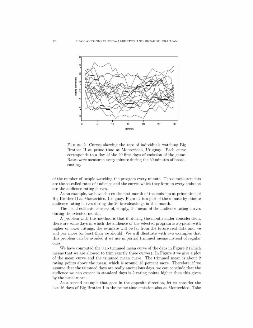
Figure 2. Curves showing the rate of individuals watching BigBrother II at prime time at Montevideo, Uruguay. Each curvecorresponds to a day of the 20 first days of emission of the game.Rates were measured every minute during the 30 minutes of broad-casting.

of the number of people watching the program every minute. Those measurementsare the so-called rates of audience and the curves which they form in every emissionare the audience rating curves.

As an example, we have chosen the first month of the emission at prime time ofBig Brother II at Montevideo, Uruguay. Figure 2 is a plot of the minute by minuteaudience rating curves during the 20 broadcastings in this month.

The usual estimate consists of, simply, the mean of the audience rating curvesduring the selected month.

A problem with this method is that if, during the month under consideration,there are some days in which the audience of the selected program is atypical, withhigher or lower ratings, the estimate will be far from the future real data and wewill pay more (or less) than we should. We will illustrate with two examples thatthis problem can be avoided if we use impartial trimmed means instead of regularones.

We have computed the 0.15 trimmed mean curve of the data in Figure 2 (whichmeans that we are allowed to trim exactly three curves). In Figure 3 we give a plotof the mean curve and the trimmed mean curve. The trimmed mean is about 2rating points above the mean, which is around 15 percent more. Therefore, if weassume that the trimmed days are really anomalous days, we can conclude that theaudience we can expect in standard days is 2 rating points higher than this givenby the usual mean.

As a second example that goes in the opposite direction, let us consider thelast 16 days of Big Brother I in the prime time emission also at Montevideo. Take


Figure 3. Mean and 15 % Trimmed Mean of the curves shown inFigure 2

.

Figure 4. Mean and trimmed mean of the 16 curves containingthe rates of the individuals watching Big Brother I at Montev-ideo, Uruguay, during the last 16 days of the game. The trimmingproportion was 3/16.

α = 3/16 (in order to trim exactly three curves) and let us see the difference betweenthe mean and the α trimmed mean. Those curves appear in Figure 4. This time,the average curve is about 2 points above the trimmed mean.

Now, the question is: Did something unusual happened on the trimmed days?The answer for the second example is rather obvious. The three trimmed curves


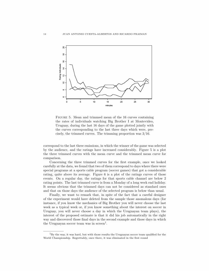
Figure 5. Mean and trimmed mean of the 16 curves containingthe rates of individuals watching Big Brother I at Montevideo,Uruguay, during the last 16 days of the game plotted jointly withthe curves corresponding to the last three days which were, pre-cisely, the trimmed curves. The trimming proportion was 3/16.

correspond to the last three emissions, in which the winner of the game was selectedby the audience, and the ratings have increased considerably. Figure 5 is a plotthe three trimmed curves with the mean curve and the trimmed mean curve forcomparison.

Concerning the three trimmed curves for the first example, once we lookedcarefully at the data, we found that two of them correspond to days where there werespecial programs at a sports cable program (soccer games) that got a considerablerating, quite above its average. Figure 6 is a plot of the ratings curves of thoseevents. On a regular day, the ratings for that sports cable channel are below 2rating points. The last trimmed curve is from a Monday of a long week end holiday.It seems obvious that the trimmed days can not be considered as standard onesand that on those days the audience of the selected program is below than usual.

Finally, we want to remark that, in spite of the fact that a careful designerof the experiment would have deleted from the sample those anomalous days (forinstance, if you know the mechanics of Big Brother you will never choose the lastweek as a typical week or, if you know something about the interest on soccer inUruguay, you will never choose a day in which the Uruguayan team plays), theinterest of the proposed estimate is that it did his job automatically in the rightway and discovered those final days in the second example and those days in whichthe Uruguayan soccer team was in screen1.

1By the way, it was hard, but with those results the Uruguayan soccer team qualified for theWorld Championship. Regrettably, once there, it was eliminated in the first round


Figure 6. Curves showing the rate of individuals watching Ten-field channel at Montevideo, Uruguay, on the 14/08/2001 and the23/08/2001 during the time at which Big Brother II was on thescreen.

7. Appendix

The first lemma is a property of uniformly convex Banach spaces and it isstated here for further reference.

Lemma 7.1. Let xn ⊂ E be a sequence which converges weakly to x0. Then(P.1) lim inf ||xn|| ≥ ||x0||.(P.2) If lim ||xn − x0|| 6= 0, then lim inf ||xn|| > ||x0||.

Proposition 7.2. Let α ∈ (0, 1) and let P be a probability measure on E. Letxn, n = 0, 1, ... ⊂ E be such that

lim ||xn − x0|| = 0 and lim rα(xn) = rα(x0).Then

lim∫||y − xn||2τxn(y)dP (y) =

∫||y − x0||2τx0(y)dP (y).

Proof. To simplify, let us denote τn = τxn . It follows easily that

lim τn(y) =

1 if y ∈ B(x0, rα(x0))

0 if y /∈ B(x0, rα(x0)).On the other hand

1− α = lim∫

τn(y)dP (y)

= lim∫ (

IB(x0,rα(x0)) + IBc(x0,rα(x0))

+ IS(x0,rα(x0))

)τn(y)dP (y),


and, the bounded convergence theorem implies that

(7.1) γ := 1− α− P [B(x0, rα(x0)] = lim∫

S(x0,rα(x0))

τn(y)dP (y).

Now, since

||y − xn||2(IB(x0,rα(x0))(y) + IB

c(x0,rα(x0)

(y))

τn(y) → ||y − x0||2IB(x0,rα(x0))(y),

again the bounded convergence theorem implies that

lim[∫

||y − xn||2τn(y)dP (y)−∫||y − x0||2τ0(y)dP (y)

]= lim

∫S(x0,rα(x0))

(||y − xn||2τn(y)− ||y − x0||2τ0(y)

)dP (y)

= r2α(x0) lim

∫S(x0,rα(x0))

(τn(y)− τ0(y)) dP (y) = 0

by (7.1).

Proof of Theorem 3.6.

Proof. Let xn ⊂ E be a sequence such that

(7.2) Dα(xn, P ) → Iα(P ).

Let us denote, to simplify, τn = τxn . We start proving that both sequencesxn and rα(xn) are bounded. Take H > 0 such that

P [B(0,H)] > α,

and let δ = P [B(0,H)]− α. Thus,∫

B(0,H)τn(y)dP (y) ≥ δ for every n ∈ IN . If the

sequence is not bounded, there exists a subsequence xnk such that ||xnk

|| → ∞,and we have that

lim Dα(xnk, P ) = lim

∫||y − xnk

||2τnk(y)dP (y)

≥ lim∫

B(0,H)

||y − xnk||2τnk

(y)dP (y)

≥ lim(||xnk|| −H)2δ = ∞,

which contradicts (7.2).Boundness of rα(xn) follows from the boundness of xn and the fact that if

H∗ satisfies that P [B(0,H∗)] > 1− α, thus, rα(xn) ≤ supk ||xk||+ H∗, since

B(0,H∗) ⊂ B(xn, ||xn||+ H∗).

In consequence, without loss of generality, we can assume that there exists x0 ∈E and r0 such that the sequence xn converges weakly to x0 and lim rα(xn) = r0.Notice that rα(x0) ≤ r0. Effectively, if we denote A = lim supB(xn, rα(xn)), wehave

1− α ≤ lim supP [B(xn, rα(xn))] ≤ P (A).On the other hand, if y ∈ A, there exists a subsequence xnk

such thaty ∈ B[xnk

, rα(xnk)] for every k and therefore

r0 ≥ lim sup ||y − xnk|| ≥ ||y − x0||,


where last inequality follows from (P.1) in Lemma 7.1. Thus, A is contained in theclosed ball B(x0, r0) and, in consequence, rα(x0) ≤ r0.

Let us, at first, assume that ||xn − x0|| converges to zero. In this case

(7.3) r0 = rα(x0).

Effectively, otherwise, since

1− α ≥ lim inf P [B(xn, rα(xn)] ≥ P [B(x0, r0)],

the only remaining possibility is that P [B(x0, r0)] = 1− α. Therefore there existsr < r0 such that P [B(x0, r)] = 1− α and, from the hypothesis, we have that froman index onward

B(x0, r) ⊂ B(xn, rα(xn)),

being this inclusion strict. Thus, there exists s ∈ (r, rα(xn)) such that

B(x0, r) ⊂ B(xn, s),

from where rα(xn) ≤ s, which is not possible. In consequence, the assumptions ofProposition 7.2 are satisfied and we have that

Iα(P ) = limn

Dα(xn, P ) =∫||y − x0||2τx0(y)dP (y),

and the theorem is proved in this case.The proof will be complete if we show that ||xn − x0|| → 0 as n →∞. Define

for δ > 0 and a natural number n, the sets

Aδ := y : lim inf ||y − xn||2 > ||y − x0||2 + δAn

δ := y : ||y − xk||2 > ||y − x0||2 + δ, for every k ≥ n.

It happens that limn P (Anδ ) = P (Aδ) and, from (P.2) in Lemma 7.1, that

limδ→0+ P (Aδ) = 1. Fix δ0 > 0 such that P (Aδ0) = α + η0 with η0 > 0. Let ε > 0.There exists δ < δ0 such that P (Aδ) > 1− ε. On the other hand, from the fact that||x0|| < lim inf ||xn||, we have that, for all y ∈ E,

||y − x0||2τn(y) ≤ [2 sup ||xn||+ sup rα(xn)]2 =: R.

Therefore

lim∫ (

||y − xn||2 − ||y − x0||2)τn(y)dP (y)

= lim

[∫An

δ0

(||y − xn||2 − ||y − x0||2

)τn(y)dP (y)

+∫

“An

δ0

”c TAn

δ

(||y − xn||2 − ||y − x0||2

)τn(y)dP (y)

+∫(Aδ0)

c T(Aδ)c

(||y − xn||2 − ||y − x0||2

)τn(y)dP (y)

]≥ lim

n[δ0η0 −Rε] ,


and taking limits on ε , we finally have that

Iα(P ) = lim∫||y − xn||2τn(y)dP (y)

≥ δ0η0 + lim∫||y − x0||2τn(y)dP (y)

≥ δ0η0 +∫||y − x0||2τx0(y)dP (y),

which contradicts the definition of Iα(P ).

In our proof of Theorem 3.7 we will employ the very well known Skorohodrepresentation theorem which we state here for the sake of completeness.

Lemma 7.3. Let Pn be a sequence of probability measures which convergesin distribution to the probability measure P . Then, there exist a probability space(X ,S, ν) and a sequence of E-valued random elements Yn : n = 0, 1, ... definedon it such that

(1) The distribution of Y0 is P and for n ≥ 1 the distribution of Yn is Pn.(2) The sequence Yn converges ν-almost surely to Y0.

Proposition 7.4. Let α ∈ (0, 1) and let Pn be a sequence of probabilitymeasures which converges in distribution to the probability measure P . Then it issatisfied that

lim sup Iα(Pn) ≤ Iα(P ).

Proof. Given r > 0, the function

y :→ ||y −mP ||2IB(mP ,r)(y)

is bounded and, if P [S(mP , r)] = 0 it is also P -a.e. continuous.Let us assume that P [B(mP , rα(mP ))] = 1 − α. Therefore, we can take

τmP= IB(mP ,rα(mP )). Let r > rα(mP ) be such that P [S(mP , r)] = 0 and that

P [B(mP , r)] > 1− α. We have that

lim sup Iα(Pn) ≤ lim sup∫

B(mP ,r)

||y −mP ||2dPn(y)

=∫

B(mP ,r)

||y −mP ||2dP (y),

and, if we take limits on r, we obtain that

lim sup Iα(Pn) ≤ Iα(P ).

Now, let us assume that P [B(mP , rα(mP ))] > 1− α. By definition of rα(mP ),if s < rα(mP ), then P [B(mP , s)] < 1− α.

Let s < rα(mP ) < r be such that P [S(mP , s)] = P [S(mP , r)] = 0. Therefore,there exists n0 ∈ IN such that if n ≥ n0, then

Pn[B(mP , s)] < 1− α < Pn[B(mP , r)].

From an index onward, there exists τnr,s a trim at level α for Pn such that

IB(mP ,s) ≤ τnr,s ≤ IB(mP ,r).


We have that

lim sup Iα(Pn) ≤ lim sup∫||y −mP ||2τn

r,s(y)dP (y)

≤ lim∫

B(mp,s)

||y −mP ||2τnr,s(y)dPn(y)

+r2(1− α− Pn[B(mp, s)]

)=

∫B(mp,s)

||y −mP ||2dP (y) + r2(1− α− P [B(mp, s)]

).

From here, if we take limits, simultaneously, on s → rα(mP ) and r → rα(mP ),we have that

lim sup Iα(Pn) ≤∫

B(mp,rα(mP ))

||y −mP ||2dP (y)

+r2α(mP ) (1− α− P [B(mP , rα(mP ))])

=∫||y −mP ||2τ(y)dP (y),

where, if we take

h =1− α− P [B(mP , rα(mP ))]

P [B(mP , rα(mP ))]− P [B(mP , rα(mP ))]the function τ is just

τ(y) =

1 if y ∈ B(mP , rα(mP )),0 if y /∈ B(mP , rα(mP )),h if y ∈ S(mP , rα(mP )),

i.e. τ is a trim at level α for P and the proposition is proved.


Proof. Let H > 0 be such that P [B(mP ,H)] > α and that [S(mP ,H)] = 0.By hypothesis, from an index onward,

Pn[B(mP ,H)] > α.

Thus, taking into account Proposition 7.4, we can apply a similar argumentto the one developed in Theorem 3.6 to show that both sequences mn and rnare bounded. Therefore, the theorem will be proved if we show that every weaklyconvergent subsequence of mn converges in norm and its limit is mP , and thatevery convergent subsequence of rn converges to rα(mP ).

Our first step is to show that if a subsequence mnk converges weakly to m,

then lim ||mnk− m|| = 0 is satisfied. To prove this, let us assume that mnk

isa subsequence which does not satisfy this property and let Yn, n = 0, 1, 2, ... bethe sequence of r.e.’s obtained applying Lemma 7.3 to Pn and P . We would havethat

lim inf ||Ynk(t)−mnk

|| > ||Y0(t)−m|| = lim ||Ynk(t)−m||,

for ν-a.e. t ∈ X . Thus, if we consider the sets

Aδ := y : lim inf ||Ynk−mnk

|| > lim ||Ynk−m||+ δ

Ahδ := y : ||Ynk

−mnk|| > ||Ynk

−m||+ δ, for every k ≥ h.we can use a similar argument to the one in Theorem 3.6 to obtain a contradiction.


Let now mnk be a subsequence which converges in norm to m ∈ E. Take

a subsequence mn′k such that there exists r0 = limk→∞ rn

′k. With the same

argument as in (7.3) we get that r0 = rα(m). On the other hand, if we take s < r0

and t ∈ X such that Y0(t) ∈ B(m, s), then

||Yn′k(t)−mn

′k||2τn

′k(Yn

′k(t)) → ||Y0(t)−m||2.

Therefore with a similar argument to the one used at the final part of the proofof Proposition 7.4 we obtain that there exists a trim at level α for P , τ , such that

lim inf Iα(Pn) = lim inf∫||y −mn

′k||2τn

′k(y)dPn(y)

= lim inf∫||Yn

′k(t)−mn

′k||2τn

′k(Yn

′k(t))dν(t)

=∫||Y0(t)−m||2τ(Y0(t))dν(t)

=∫||y −m||2τ(y)dP (y)

≥ Iα(P ),(7.4)

where τ is defined as in Proposition 7.4. Therefore, Proposition 7.4 implies thatm = mP and that τ = τP .

It remains to show that lim rn = r(P ). But this has been already proved,because, in fact, we have shown that the whole sequence rn is bounded and thatevery convergent subsequence of it converges to rα(mP , P ).

Proof of Corollary 3.9.

Proof. We will employ the same notation as in Theorem 3.7. Let us considera strictly increasing sequence of natural numbers nk. According to Remark 3.8,there exists a subsequence n′

k such that the sequence mn′k converges in norm

to an α-trimmed mean of P , mP .Therefore, if we apply (7.4) to this subsequence, we have that

lim inf Iα(Pn′k) ≥ Iα(P ).

By Proposition 7.4, we have that every subsequence of Iα(Pn) containsa further subsequence which converges to Iα(P ). But this is impossible unlesslim Iα(Pn) = Iα(P ).


Proof. Given z = (z1, ..., zn) ∈ En or z = (z1, z2, ...) ∈ E∞, let us denote bymn(z) the α-trimmed mean of the probability measure P z

n = n−1∑

i≤n δzi .Let us suppose that the theorem does not hold. If so, there exists A ⊂ E∞

with P∞(A) > 0 and such that if x ∈ A, then mn is not resistant at x.According to Theorem 3.10, the set

B := x ∈ E∞ : mn(x) → mP

satisfies that P∞(B) = 1. Without loss of generality we can also assume that forevery x ∈ B, the sequence P x

n converges in distribution to P .


Now, let x ∈ A ∩ B. According to the definition, there exists ε > 0 and threesequences δk, nk and ynk

such that δk > 0 and lim δk = 0; nk ∈ IN andlim nk = ∞ and dnk

(xnk, ynk

) < δk and ||mnk(xnk

)−mnk(ynk

)|| > ε.By Lemma 2.1 in [3], we have that if ρ denotes for the Prohorov metric, then

limk

ρ(P xnk

, Pynknk ) = 0,

and in consequence, we have that the sequence of probability measures P ynknk

converges weakly to P . Thus, according to Theorem 3.7, we have also that

limk

mnk(ynk

) = mP ,

what gives a contradiction with the fact that ||mnk(xnk

)−mnk(ynk

)|| > ε for everyk.

In order to prove Theorem 4.4, we need to introduce some additional notation.Given A ⊂ E and n ∈ IN , An will be the projection of A on the subspace generatedby e1, ..., en, An,1 its projection on the subspace generated by e2, ..., en, andA∞,n the projection on the subspace generated by en+1, en+2, .... −A will be thesymmetrical set of A with respect to 0 and the subspace e2, e3, ...; while, givenδ ∈ IR,

Aδ := x + δe1 : x ∈ A.

Given x ∈ E we will denote, for instance xn = xn and so on. We will abuseof notation and An,1 will also stand for the coordinates set (in Rn) with respect tothe fixed orthonormal basis of E of the set A.

The proof of Theorem 4.4 will be based on the following two propositions.

Proposition 7.5. Under the hypotheses in Theorem 4.4, if A ⊂ E is a closedand bounded set such that there exists δ > 0 satisfying that A1 + δ ⊂ IR−, thenP [Aδ] > P [A].

Proof. Notice that the hypothesis implies that A1 ⊂ IR−. Therefore, theassumptions imply that if a ∈ A1, then f1(a + δ) > f1(a). Moreover, since A isbounded, we have that A1 is compact and there exists η > 1 such that

infa∈A1

f1(a + δ)/f1(a) ≥ η,

which implies that

P [(An)δ] =∫

An

f1(x1 + δ)f2(x2)...fn(xn)dx1...dxn

≥ η

∫An

f1(x1)f2(x2)...fn(xn)dx1...dxn = ηP (An).

Having in mind that η depends only on A1 but not on n, we obtain the resultjust by taking limits on n.

Proposition 7.6. Let us assume the hypotheses in Theorem 4.4. Let r > 0.If m ∈ E satisfies that m1 6= 0, then

(7.5) P [B(m∞,1, r)] > P [B(m1, r)].


Proof. Let r > 0 and m ∈ E be such that m1 > 0 (the other case is analo-gous). Let us consider the half-balls

B− = B(m, r) ∩ x : x1 ≤ m1 and B+ = B(m, r) ∩ x : x1 > m1.

The proof consists on performing some transformations (symmetries and trans-lations) of B− and B+ or some subsets of them. Those transformations depend onr. Thus, we need to split the proof according to the possible values of r. Let usassume at first that r ≤ m1/2.

By the symmetry assumption, P [B+] = P [−B+]. Moreover, (−B+)1 + m1 ⊂IR− and, by Proposition 7.5, we have that

P [(−B+)m1 ] ≥ P [B+].

On the other hand, let us call S(B−) the image of the half-ball B− by the sym-metry determined by the point m− re1 and the subspace generated by e2, e3, ....It follows that, (S(B−))1 ⊂ IR+ and P [S(B−)] ≥ P (B−). On the other hand,S(B−)2r−m1

1 ⊂ IR+ and, by Proposition 7.5, P [S(B−)] ≤ P [S(B−)2r−m1 ].Therefore (7.5) is shown in this case since

B(m∞, r) = (S(B−))2r−m1 ∪ (−B+)m1 ,

and the sets in the right hand side are disjoint.The next case to be considered is m1/2 < r ≤ m1. In this case we handle B+

in the same way as in the previous case. The difference is related to B− becausenow S(B−)1 ∩ IR− 6= ∅. Thus, let us consider the point

m∗ := m− m1

2e1,

and let S∗ denote the symmetry determined by m∗ and the subspace generated bye2, e3, .... Let

C := B− − [B− ∩ S∗(B−)].

Notice that P [S∗(C)] > P [C]. Then the proof is also complete in this casesince now

B(m∞,1, r) = S∗(C) ∪ (B− ∩ S∗(B−)) ∪ (−B+)m1 .

Finally let’s consider the case m1 < r. Here we need to decompose

B− = B−,1 ∪B−,2 := x ∈ B−x1 ≥ 0 ∪ x ∈ B−x1 < 0.

We apply to B−,1 the same transformation as we did to B− in the second case.i.e. we consider

C1 := B−,1 −B−,1 ∩ S∗(B−,1),

and handle C1 as C in previous case, while B−,1 ∩ S∗(B−,1) remains fixed.Concerning B+, let us denote C2 = S∗(B−,2). Obviously C2 ⊂ B+. C2 will

also remain fixed. The only remaining part is B+ ∩ (C2)c. Since

P [B+ ∩ (C2)c] < P [−(B+ ∩ (C2)c)m1 ],

the proof follows since in this case, we have the decomposition

B(m∞,1, r) = [(−(B+ ∩ (C2)c))m1 ] ∪ C2 ∪ S∗(C1) ∪ (B−,1 ∩ (C1)c).



Proof. Let r > 0 and let m ∈ E, m 6= 0. According to Proposition 7.6, ifmn 6= 0 then

P [B(m∞,n−1, r)] < P [B(m∞,n, r)],while, if mn = 0, m∞,n−1 = m∞,n.

Thus, we have the inequalities

P [B(m, r)] ≤ P [B(m∞,1, r)] ≤ P [B(m∞,2, r)] ≤ . . .

where at least one of them is strict. On the other hand lim ||m∞,n|| = 0 and wehave that

P [B(m, r)] < lim P [B(m∞,n, r)] ≤ P [lim sup B(m∞,n, r)] = P [B(0, r)].

The proof of the Theorem 5.1 will be based on the following proposition.

Proposition 7.7. Let us assume that the hypothesis in Theorem 3.7 hold. Letxn ⊂ E be a sequence such that lim ||xn −mP || = 0. Then

lim supDα(xn, Pn) ≤ Iα(P ).

Proof. Given n ∈ IN , let mn be a trimmed mean of Pn. By Theorem 3.7 wehave that lim ||mn −mP || = 0 and that limn rn = r(P ). Thus lim ||mn − xn|| = 0and, if we denote R := sup(rn), it follows that

||y −mn||τn(y) ≤ Rτn(y).

Therefore we have that

Dα(xn, Pn) ≤∫||y − xn||2τn(y)dP (y)

≤ Dα(mn, Pn) +[||mn − xn||2 + 2||mn − xn||R

](1− α)

= Iα(Pn) +[||mn − xn||2 + 2||mn − xn||R

](1− α),

which, together with Corollary 3.9, gives the result.


Proof. By the extension of the Glivenko-Cantelli Theorem there exists a µ-probability one set Ω0 such that if ω ∈ Ω0, then mP belongs to the closure of theset X1(ω), X2(ω), ... and the sequence Pn converges in distribution to P .

Let us fix ω ∈ Ω0. Given n ∈ IN , there exists Xin(ω) ∈ X1(ω), ..., Xn(ω)such that ||Xin(ω)−mP || → 0. Therefore we have that

(7.6) lim sup Iα(Pn) ≤ lim supDα(Xin(ω), Pn) ≤ Iα(P ),

where last inequality is a consequence of Proposition 7.7.Now (7.6) is a starting point analogous to the conclusion of Proposition 7.4

which, if we make here the same reasoning as in Theorem 3.7, allows to obtain thedesired result.

ACKNOWLEDGMENTS. This research was started during a visit of the firstauthor to the Universidad de la Republica del Uruguay. He wants to thank forthe warm hospitality received there. This stay was supported by a grant from theUniversidad de Cantabria.

The present version have been completed during a visit of the second authorto the Universidad de Cantabria. This stay has been supported by the Instituto


de Cooperacion Iberoamericana, Programa de Cooperacion Interuniversitaria AL-E2003.

We would also want to thank to Mediametrıa TV, Corporacion Combex, forproviding the TV rating data.

References

[1] P. BESSE and J.O. RAMSAY, Principal component analysis of sampled functions. Psy-chometrika 51 (1986), 285-311.

[2] G. BOENTE and R. FRAIMAN, Kernel-based functional principal components. Statist.Probab. Lett. 48 (2000), 335-345 .

[3] G. BOENTE, FRAIMAN, R. and V.J. YOHAI, Qualitative Robustness for Stochastic Pro-cesses. Ann. Statist. 15 (1987), 1293-1312.

[4] D. BOSQ, Modelization, non-parametric estimation and prediction for continuous time pro-cesses. Nonparametric Functional Estimation and Related Topics, G.G. Roussas et al. eds.,Kluwer Academic Publishers, 1991, 509-529.

[5] B.M. BROWN. Statistical uses of the spatial median. J. Roy. Statist. Soc. Ser. B, 45 (1983),25-30.

[6] B.A. BRUMBACK and J.A. RICE, Smoothing spline models for the analysis of nested andcrossed samples of curves (with discussion) J. Amer. Statist. Assoc., 93 (1998), 961-994.

[7] D. COX, Metrics on stochastic processes and qualitative robustness Technical Report 3. Dept.Statistics, Univ. Washington, 1981.

[8] J.A. CUESTA-ALBERTOS, A. GORDALIZA and C. MATRAN. Trimmed k-Means: AnAttempt to Robustify Quantizers. Ann. Statist., 25 (1997), 553-576.

[9] J.A. CUESTA-ALBERTOS, A. GORDALIZA and C. MATRAN, Trimmed best k-nets: Arobustified version of an L∞–based clustering method. Statist. Probab. Lett., 36 (1998),401-413.

[10] J. A. CUESTA and C. MATRAN. The Strong Law of Large Numbers for k-Means andBest Possible Nets of Banach Valued Random Variables. Probab. Theory Related Fields, 78(1988), 523-534.

[11] J.A. CUESTA-ALBERTOS, C. MATRAN, C. and A. MAYO-ISCAR. Stem-cell based esti-mators in the mixture model. Technical report, 2003.

[12] A. CUEVAS, M. FEBRERO and R. FRAIMAN. Linear functional regression: the case offixed design and functional response. Unpublised manuscript, 2001.

[13] J. DAUXOIS, A. POUSSE and Y. ROMAIN. Asymptotic theory for principal componentsanalysis of a vector random function: some applications to statistical inference. J. Multi-variate Anal. 12 (1982), 136-154.

[14] D.L. DONOHO and M. GASKO. Breakdown properties of location estimates based on halfs-pace depth and projected outlyingness. Ann. Statist. 20 (1992), 1803-1827.

[15] J. FAN and S.K. LIN. Test of significance when the data are curves. J. Amer. Statist. Assoc.93 (1998), 1007-1021.

[16] F. FERRATY. and P. VIEU. Functional nonparametric model for scalar response. Manu-script, 1999.

[17] D. FRAIMAN. Un analisis de la estructura de consumo electrico en Buenos Aires.TechnicalReport, 2001.

[18] R. FRAIMAN and J. MELOCHE. Multivariate L-estimation (with discussion). Test 8 (1999),255-317.

[19] R. FRAIMAN and G. MUNIZ. Trimmed means for functional data. Test, 10 (2001), 419-440.

[20] R. FRAIMAN and G. PEREZ IRIBARREN. Nonparametric regression estimation in modelswith weak error’s structure. J. Multivariate Anal. 21 (1991), 180-196.

[21] L.A. GARCIA-ESCUDERO, A. GORDALIZA and C. MATRAN. A central limit theoremfor multivariate generalized trimmed k-means. Ann. Statist. 27 (1999), 1061-1079.

[22] A. GORDALIZA. Best approximations to random variables based on trimming procedures.J. Approx. Theory 64 (1991), 162-180.

[23] F.R. HAMPEL. A general qualitative definition of robustness. Ann. Math. Statist. 42 (1971),1887-1896.


[24] J.D. HART and T.E. WEHRLY. Kernel regression estimation using repeated measurementdata. J. Amer. Statist. Assoc. 81 (1986), 1080-1088.

[25] T. HASTIE and R. TIBSHIRANI. Varying-coefficient models. J. Royal Statist. Soc., SeriesB 55 (1993), 757-796.

[26] A. KNEIP and T. GASSER. Statistical tools to analyze data representing a sample of curves.Ann. Statist., 20 (1992), 1266-1305.

[27] R. LIU. On the notion of simplicial depth. Proceedings of the National Academy of Sciences,U.S.A., 85 (1988), 1732-1734.

[28] R. LIU. On a notion of data depth based on random simplices. Ann. Statist. 18 (1990),405-414.

[29] R. LIU and K. SINGH. A quality index based on data depth and multivariate rank tests. J.Amer. Statist. Assoc., 421 (1993), 252-260.

[30] N. LOCANTORE, J.S. MARRON, D.G. SIMPSON, N. TRIPOLI, J. T. ZHANG and K.L.COHEN. Robust principal component analysis for functional data (with discussion). Test 8(1999), 1-74.

[31] P.C. MAHALANOBIS. On the generalized distance in statistics. Proceedings of the NationalAcademy of India, 12 (1936), 49-55.

[32] A. MAYO. Estimacion de Parametros en Mezclas de Poblaciones Normales no Homogeneas.Ph. D. Thesis. Universidad de Valladolid. Spain, 2001.

[33] K. MOSLER. Multivariate Dispersion, Central Regions and Depth. The Lift Zonoid Ap-proach. Lecture Notes in Statistics, 165. Springer, New York, 2002.

[34] H. OJA. Descriptive statistics for multivariate distributions. Statist. Probab. Lett. 1 (1983),327-332.

[35] P. PAPANTONI-KAZAKOS and R.M. GRAY. Robustness of estimates on stationary obser-vations. Ann. Probab., 7 (1979), 989-1002.

[36] J.O. RAMSAY. When the data are functions. Psychometrika , 47 (1982), 379-396.[37] J.O. RAMSAY and C.J. DALZELL. Some tools for functional data analysis (with discussion).

J. Roy. Statist. Soc. Ser. B, 52 (1991), 539-572.[38] J.O. RAMSAY and B.W. SILVERMAN. Functional Data Analysis. Springer Series in Sta-

tistics, Springer, New York, 1997.[39] J.O. RAMSAY and B.W. SILVERMAN. Applied Functional Data Analysis. Springer Series

in Statistics, Springer, New York, 2002.[40] J. RICE and B.W. SILVERMAN. Estimating the mean and covariance structure nonpara-

metrically when data are curves. J. Roy. Statist. Soc. Ser. B 53 (1991), 233-243.[41] C.G. SMALL. A survey of multidimensional medians. Internat. Statist. Rev. 58 (1990), 263-

277.[42] K. SINGH. A notion of majority depth. Technical Report. Rutgers University, Department

of Statistics, 1991.[43] J.W. TUKEY. Mathematics and picturing data. Proceedings of the International Congress

of Mathematics, Vancouver, 2 (1975), 523-531.[44] A.W. van der VAART and J. A. WELLNER Weak Convergence and Empirical Processes.

Springer Series in Statistics. Springer, New York, 1996.

Departamento de Matematicas, Estadıstica y Computacion, Facultad de Ciencias.Avda. los Castros s.n., 39005 SANTANDER, Spain

E-mail address: [email protected]

Departamento de Matematica y Ciencias, Universidad de San Andres, Argentina2

E-mail address: [email protected]

2On leave Centro de Matematica, Universidad de la Republica, Uruguay.

Impartial Trimmed Means for Functional Data

Documents