Impacts of measured data uncertainty on urban stormwater models

Journal of Hydrology 508 (2014) 28–42

Contents lists available at ScienceDirect

Journal of Hydrology

journal homepage: www.elsevier .com/locate / jhydrol

Impacts of measured data uncertainty on urban stormwater models

0022-1694/$ - see front matter � 2013 Elsevier B.V. All rights reserved.http://dx.doi.org/10.1016/j.jhydrol.2013.10.025

⇑ Corresponding author. Address: Department of Civil Engineering, Building 60,Monash University, VIC 3800, Australia. Tel.: +61 3 9905 5022.

E-mail address: [email protected] (C.B.S. Dotto).

C.B.S. Dotto a,⇑, M. Kleidorfer a, A. Deletic a, W. Rauch b, D.T. McCarthy a

a Monash Water for Liveability, Monash University, VIC 3800, Australiab Unit of Environmental Engineering, Faculty of Civil Engineering, University of Innsbruck, Technikerstrasse 13, A-6020 Innsbruck, Austria

a r t i c l e i n f o

Article history:Received 21 January 2013Received in revised form 10 October 2013Accepted 16 October 2013Available online 25 October 2013This manuscript was handled by AndrasBardossy, Editor-in-Chief, with theassistance of Vazken Andréassian, AssociateEditor

Keywords:Input and calibration dataUrban drainageModelling measurement errorsSensitivity analysisBayesian inferenceParameter probability distributions

s u m m a r y

Assessing uncertainties in models due to different sources of errors is crucial for advancing urbandrainage modelling practice. This paper explores the impact of input and calibration data errors on theparameter sensitivity and predictive uncertainty by propagating these errors through an urbanstormwater model (rainfall runoff model KAREN coupled with a build-up/wash-off water quality model).Error models were developed to disturb the measured input and calibration data to reflect commonsystematic and random uncertainties found in these types of datasets. A Bayesian approach was usedfor model sensitivity and uncertainty analysis. It was found that random errors in measured data hadminor impact on the model performance and sensitivity. In general, systematic errors in input and cali-bration data impacted the parameter distributions (e.g. changed their shapes and location of peaks). Inmost of the systematic error scenarios (especially those where uncertainty in input and calibration datawas represented using ‘best-case’ assumptions), the errors in measured data were fully compensated bythe parameters. Parameters were unable to compensate in some of the scenarios where the systematicuncertainty in the input and calibration data were represented using extreme worst-case scenarios. Assuch, in these few worst case scenarios, the model’s performance was reduced considerably.

� 2013 Elsevier B.V. All rights reserved.

1. Introduction and background

Stormwater models underpin the decision making process inurban water management, policies and regulations. Moreover, theyare key tools for the quantification of urban discharges and also forthe design of stormwater treatment technologies. Uncertainties,however, are intrinsic to all models and it is hypothesised thatthe level of accuracy of any model’s output is often compromisedif the different sources of errors are not considered during themodelling exercise. Therefore, assessing uncertainties in modelsdue to different sources of errors is crucial for advancing urbandrainage modelling practice. Typically, three sources of randomand systematic uncertainties are identified: errors in the measuredinput and calibration data, and errors due to incomplete or biasedmodel structure (Butts et al., 2004). While the uncertainty in thecalibrated parameter values combines the different sources, theimpact of calibration and uncertainty analysis methods, differentobjective functions and calibration data availability on the modelsensitivity are also recognised (Mourad et al., 2005; Dotto et al.,2012; Kleidorfer et al., 2012).

As with most models, the calibration of urban drainage modelsrarely results in one unique parameter set, and instead many

equally plausible parameter sets are obtained, which reduces theconfidence in the models when they are used for prediction(Kuczera and Parent, 1998). The uncertainty related to the modelcalibration parameters and its impact on the model outputs hasbeen extensively studied (e.g. Kanso et al., 2003; Feyen et al.,2007). Global sensitivity analysis methods have been applied toestimate the confidence intervals around the model’s predictionwhile revealing the sensitivity of the model outputs to each param-eter (e.g. Feyen et al., 2007; Yang et al., 2008). Many methodologiesare available to conduct these uncertainty/sensitivity analyses,including informal Bayesian methods (e.g. GLUE by Beven andBinley (1992)) and formal Bayesian approaches (e.g. MICA byDoherty (2003) and DREAM by Vrugt et al. (2009)). Comparisonshave been made between these methods in various research areas(e.g. Yang et al., 2008; Matott et al., 2009), including urban drain-age modelling (Dotto et al., 2012). These comparisons suggest thatmodellers should choose the method which is most suitable for thesystem they are modelling (e.g. complexity of the model’sstructure including the number of parameters), their skill andknowledge level, the available information, and the purpose oftheir study.

Measured data such as rainfall, flow rates and pollutant concen-trations are needed for the application of urban drainage models.While rainfall data is the main input for most urban drainage mod-els, flow rates and pollution concentration data are required formodel calibration and validation. These measured datasets have

C.B.S. Dotto et al. / Journal of Hydrology 508 (2014) 28–42 29

inherent uncertainty and it has been shown that this uncertaintyincreases the data requirements for model calibration (Mouradet al., 2005). The input data used in stormwater modelling couldbe highly uncertain. For example, the main sources of uncertaintiesin rainfall intensities, commonly measured using tipping bucketrain gauges, are related to both rainfall catching and counting er-rors (Molini et al., 2005b). While splashing losses were found tobe only up to 2% and evaporation losses were up to 4%, the windlosses were found to be inversely proportional to the rain intensityand were up to 30% for rainfall intensities around 0.25 mm/h(Sevruk, 1982; Rauch et al., 1998; Einfalt et al., 2002). Battery, log-ger and computer clock failures are also significant source of errorsin rainfall measurements. For example, time drifts are inherent toany battery controlling logging device and values around 0.07 min/day were reported by McCarthy (2008). The spatial variability ofrainfall often is a large source of errors when point source mea-surement methods are used (such as tipping bucket gauges). To ad-dress this issue radar rainfall data can be used to estimateprecipitation, but radar data is also subject of several assumptionsthat introduce a number of errors For example, Krajewski et al.(2010) also report differences of up to 30% by comparing radarand rain gauges for 20 investigated storm events.

While addressed in related fields (e.g. hydrologic models:Krzysztofowicz and Kelly, 2000; Haydon and Deletic, 2009), theimpacts of input data uncertainties on urban drainage models arelargely unknown. Only a few studies evaluated the propagationof input data uncertainties through urban drainage models (Rauchet al., 1998; Bertrand-Krajewski et al., 2003) and in all of them, themodels were first calibrated assuming that measured inputs andoutputs are without error, and the impacts of input data uncertain-ties were then propagated through the models, while keeping themodel parameters fixed. Kleidorfer et al. (2009) developed this fur-ther by assessing the impact of input data uncertainties on modelparameters and found that the parameters of both flow and pollu-tion models were influenced by systematic errors in input data.

In addition, the techniques used to measure urban dischargesand associated water quality parameters, that are needed forcalibration of stormwater models, also contain error (Bertrand-Krajewski et al., 2003; Harmel et al., 2006; McCarthy et al.,2008). For example, uncertainties in stormwater flow data, com-monly measured using velocity-area measurement method, rangefrom 2% to 20% (Harmel et al., 2006). While these random errorscan be estimated, uncertainties in flow measurements due to sys-tematic errors (often related to the height measurement and inac-curate velocity calibration or incorrect probe set-up) were notexplored (Harmel et al., 2006).

Errors in water quality data are far larger than for flows or rain-fall. Sampling, storage and analytical/laboratory methods all haveinherent errors which contribute to the uncertainty in the finalsample’s pollutant concentration (Harmel et al., 2006). While sam-pling errors, related to the position of the probe, are significant intotal suspended solids (TSS) measurements, with values up to 33%,they are not significant for dissolved pollutants that do not settle(Harmel et al., 2006). Some dissolved pollutants are more impactedby storage uncertainties; values up to 49% were reported for totalnitrogen (TN) even for samples which are kept iced and are ana-lysed within 6 h (Kotlash and Chessman, 1998). Uncertainty re-lated to the laboratory analysis was less explored, but valuesfrom �9.8% to 5.1% have been reported for TSS (Harmel et al.,2006). Although these uncertainties are acknowledged in the urbandrainage field, the impact of them on stormwater models has notbeen explored.

In addition, the combined impact of input and calibration dataon urban stormwater models is unknown. However, valuable infor-mation can be obtained from related studies on modelling of largenatural catchments. For example, Renard et al. (2008) and Thyer

et al. (2009) applied the Bayesian Total Error Analysis methodology(BATEA proposed by Kuczera et al. (2006)) to evaluate the uncer-tainties in hydrological models arising from model input, outputand structural errors. The BATEA framework is based on hierarchi-cal Bayesian models and is very comprehensive and transferable(Renard et al., 2008). However, it is rather difficult for application,since it requires a large number of extra calibration parameters(that are associated with modelling the errors), is computationallydemanding, and requires a significant level of understanding of thetested model structure and the of the assumed error models(Renard et al., 2008).

In summary, the combined effect of input and calibration datauncertainty on the parameters and outputs of urban drainage mod-els has not been explored. Recently, the International WorkingGroup on Data and Models of the Joint Committee on Urban Drain-age that works under IWA and IAHR proposed an overarchingframework that could address this issue (Deletic et al., 2012). How-ever, the framework has never been tested, lacking practical detailson the methodology. This paper is the first attempt to test the pro-posed framework for assessing the impact of both input and cali-bration data errors on the parameter sensitivity and predictiveuncertainty of an urban rainfall runoff and water quality modelusing a rich Melbourne dataset.

2. Methods

2.1. Adopted stormwater models

Rainfall runoff model. KAREN (Rauch and Kinzel, 2007) was se-lected for the study because of its simplicity and proven perfor-mance for urbanised catchments (Kleidorfer et al., 2009). KARENis a linear reservoir model, which only requires the catchment areaand a rainfall time series as inputs to generate a series of flowsoriginating from impervious areas (Ai) only. Ai of the catchmentis calculated from total area (Atot) and the calibration parametereffective impervious fraction (EIF) as Ai = EIF � Atot. Runoff fromimpervious areas occurs after a rainfall threshold has beenexceeded (calibration parameter li). Therefore, effective rainfallhe is calculated from measured rainfall hn and li as he,j = hn,j � li,j.The initial loss is calculated continuously in each timestep j andfills during rainfall and is drained during dry weather by a perma-nent loss calibration parameter (eV) according to li,j = li,j�1 � eV.Surface runoff volume is calculated using the linear time-areamethod, which is related to the unit hydrograph method (Sherman,1932). At the beginning of a rainfall event, the effective imperviousarea is increased according to the flow time on the catchment sur-face until the whole catchment contributes to runoff after thecatchment’s time of concentration (calibration parameter TOC).Consequently the runoff Qj is calculated from he and Ai for eachtimestep j of length Dt according to Qj ¼ he;1 � Ai;j þ he;2�Ai;j�1 þ � � � þ he;k � Ai;j�kþ1 ¼

PKk¼1he;k � Ai�kþ1: The index k represents

the rainfall index ranging from 1 to K = TOC/Dt, Ai�k+1 is theeffective impervious area for the current timestep.

Water quality model. A very well researched and widely adoptedbuild-up and wash-off model (initially proposed by Sartor andBoyd (1972) was used to model TSS concentrations in catchmentsdischarges. It was selected because of its widespread use in prac-tice; e.g. it is used in SWMM (USEPA, 2007). The original modelwas slightly modified and hence the key equations are presentedin Table 1 (formatted for a 6 min timestep).

The main modification from the original is in the wash-offstage. The concentration of pollutants in the runoff within a time-step (C in mg/L) is a power function of the catchment runoff mod-elled with KAREN (q in mm/h) divided by the catchment runoffcoefficient (RC – here assumed as the EIF calibrated with KAREN).

Table 1The governing equations of the build-up/wash-off model.

Process and model equation Unit Equation no.

Build-up during dry weather: MðtdÞ ¼ M0 1� e�6k11440td

� �(kg) 1

Wash-off during wet weather: CðtÞ ¼ k2MðtdÞ qRC ðt þ rÞk3 (mg/L) 2

WðtÞ ¼ 10�6CðtÞVolðtÞ (kg) 3

M(td) is the mass of solids which accumulate on the surface during dry weather periods (td) within a timestep in kg; M0 is the maximum amount of accumulated solids in kg,k1 represents the accumulation constant in day�1; c is the concentration of pollutants in the runoff at the time t in mg/L; k2 and k3 are the wash-off coefficient and exponent,respectively; q is the runoff in mm/h, RC is the catchment runoff coefficient; and, r in number of timesteps in min is used to correct for the fact that pollutograph precedes therunoff hydrograph (Chiew and McMahon, 1999). W(t) is the wash-off of TSS from the surface; Vol is the runoff volume in L.

30 C.B.S. Dotto et al. / Journal of Hydrology 508 (2014) 28–42

RC was included to represent wash-off only from impervious sur-faces, which is a safe assumption because majority of runoff fromurban catchments are originated from impervious surfaces (Chiewand McMahon, 1999). If instead of q rainfall intensities were used,the model would have to include a routing algorithm (e.g. linearreservoir routing) resulting in an additional parameter(s). A trans-port related parameter (r) was used to represent the small lag timewhich is often noted between the hydrographs and the polluto-graphs (Vaze and Chiew, 2003). The amount of pollutants washedfrom the surface (W in kg) is then calculated in function of the pre-dicted concentration and the volume (Vol in L). In total, there are 5calibration parameters: M0, (kg), k1 (day�1); k2; k3; and, r (numberof timesteps).

2.1.1. Catchment and datasetAn urban catchment, located in Richmond, an eastern suburb of

Melbourne, Australia, was used. The site has a total area of 89 ha,the land use is high-density residential with a total imperviousnessof 74% and an average slope of less than 0.1%. The catchment isdrained by a separate stormwater system.

Rainfall is measured using a standard 0.2 mm/tip tipping gaugelocated 600 m from the catchment centroid. Flows were measuredwith the American Sigma/HACH area-velocity 950 sensor (HACH,2008) installed in the outlet pipe. The water quality samples(TSS) were also collected at the outlet of the catchments by auto-samplers using flow-based intervals and each sample being ana-lysed for TSS. Details on the catchment, monitoring program andthe datasets are available in Francey et al. (2010). Rainfall and flowdata collected between 2004 and 2005, and 44 TSS pollutographs(approximately 250 samples) were used for calibration. The eventtotal rainfall ranged from 2 to 60 mm, the mean maximum eventrunoff rate was 547 L/s and the average of the TSS Event Mean Con-centration (EMC) was 125 mg/L (The EMCs were calculated usingthe discrete TSS concentrations with their associated volumes asper Leecaster et al., 2002). Rainfall and flow data collected from2006 to 2007 were used for model validation; the event total rain-fall ranged from 2 to 44 mm and the mean maximum event runoffrate was 212 L/s. The calibration of the water quality model re-sulted in very low performance, and therefore validation of thismodel would not succeed and was not carried out.

2.2. Assessing global uncertainties

The proposed framework (Fig. 1) is a further development of thegeneral framework proposed by the International Working Groupon Data and Models (see Deletic et al., 2012). Firstly, the modelis fed with a certain set of input data (X). The model then generatesits outputs (Y) as a function of X and a set of calibration parameters(h). By means of an appropriate uncertainty analysis method and acertain objective function (OF), the model is run repeated timesuntil the misfit (e) between the measured data (O) and the mod-elled data (Y) is reduced. Through this process, the parameter prob-ability distributions (PDs) are generated. Finally, the model

predictive uncertainty bands are obtained. To test the influenceof input and calibration data uncertainties on the modelling proce-dure, both datasets were disturbed using error models. The classi-cal approach is again employed, but this time using these disturbeddatasets (disturbed input X* and calibration O* data). The parame-ter distributions and the predictive uncertainty bands producedusing these disturbed datasets are then compared with those pro-duced when using the undisturbed data; the differences are usedto assess the impacts of these errors. To become operational, thisuntested/unapplied framework, had to be developed further as ex-plained in the consequent sections.

2.2.1. Method used for uncertainty analysisA Bayesian approach was selected for evaluation of the model

parameter sensitivity, since it has some important advantageswhen used for stormwater modelling (Dotto et al., 2012). ThePDs of model parameters were generated using the outputs ofthe software package MICA (Doherty, 2003), which uses a MarkovChain Monte Carlo (MCMC) method with the Metropolis–Hastingsalgorithm sampler. The likelihood function adopted in MICA isleast square based and assumes that the residuals between themeasured and modelled values have a normal distribution (e.g.Feyen et al., 2007); as such, the measured calibration and modelleddata series were transformed using a Box–Cox transformation(Box and Cox, 1964) to achieve homoscedasticity and normally dis-tributed residuals. However, all transformation methods changethe content of the observations (Beven et al., 2008), which theninfluences the emphasis on various parts of the hydrograph (or pol-lutograph). This is sometimes not desired if the modelling purposeis to focus on specific parts of the dataset (e.g. flood prediction islinked with peak flows, which are deemphasised when usingBox–Cox transformations) (Doherty and Welter, 2010). Further-more, all observed data have uncertainty, and this should be takeninto account in the likelihood function so that the parameters areestimated appropriately; indeed, it is important that the functionplaces more emphasis on data which has lower uncertainty.Weighting strategies can be used to re-adjust how the likelihoodfunction emphasises various parts of the dataset to (1) considermeasured data uncertainty and (2) compensate for the Box–Coxtransformation which may have adjusted the emphasis in an unde-sirable way. Therefore, the weights were computed based on theinverse of the relative uncertainty in the measured (untrans-formed) data (i.e. the relative error in the measured flow rates cal-culated using the Law of Propagation of Uncertainties; seeMcCarthy et al., 2008 for more information). The serial correlationbetween the data points was not considered because the currentused methods to account for autocorrelation (e.g. first order mod-el) are not effective for small timesteps as used in this study(e.g. Yang et al., 2008; Métadier and Bertrand-Krajewski, 2012).

The performance of the model was evaluated using theNash–Sutcliffe efficiency criterion (E) (Nash and Sutcliffe, 1970)corresponding to the minimum least square value achieved withMICA. E is calculated by normalizing least squares by the variance

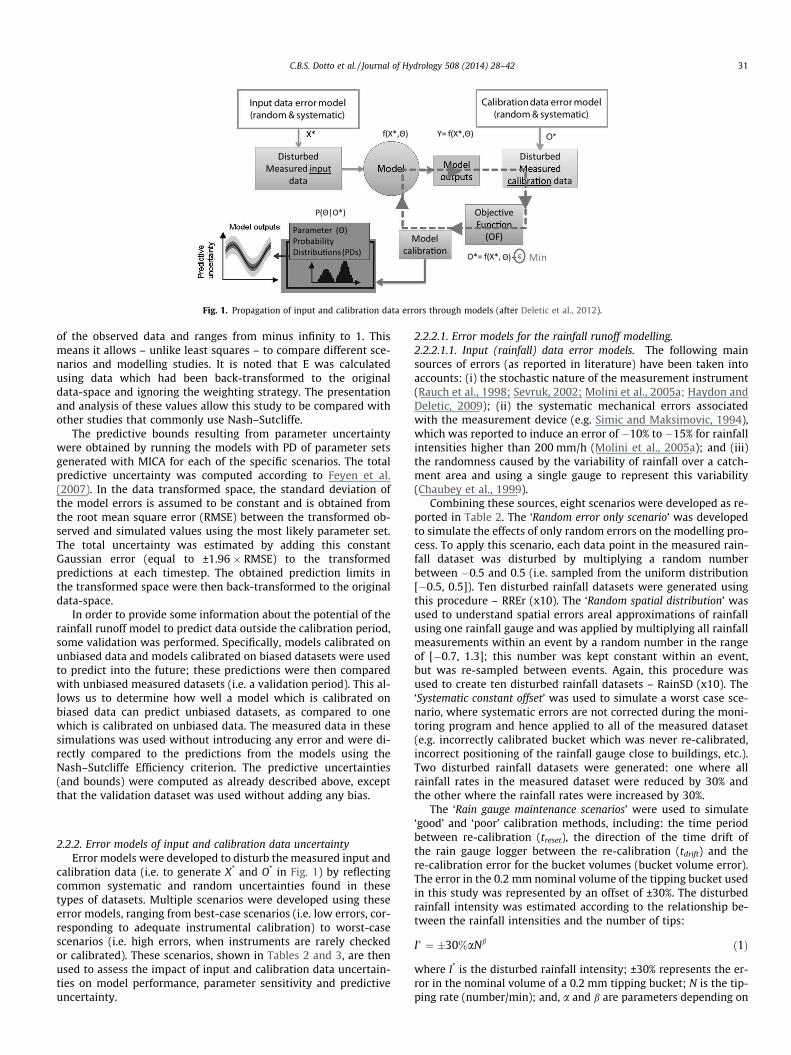
Fig. 1. Propagation of input and calibration data errors through models (after Deletic et al., 2012).

C.B.S. Dotto et al. / Journal of Hydrology 508 (2014) 28–42 31

of the observed data and ranges from minus infinity to 1. Thismeans it allows – unlike least squares – to compare different sce-narios and modelling studies. It is noted that E was calculatedusing data which had been back-transformed to the originaldata-space and ignoring the weighting strategy. The presentationand analysis of these values allow this study to be compared withother studies that commonly use Nash–Sutcliffe.

The predictive bounds resulting from parameter uncertaintywere obtained by running the models with PD of parameter setsgenerated with MICA for each of the specific scenarios. The totalpredictive uncertainty was computed according to Feyen et al.(2007). In the data transformed space, the standard deviation ofthe model errors is assumed to be constant and is obtained fromthe root mean square error (RMSE) between the transformed ob-served and simulated values using the most likely parameter set.The total uncertainty was estimated by adding this constantGaussian error (equal to ±1.96 � RMSE) to the transformedpredictions at each timestep. The obtained prediction limits inthe transformed space were then back-transformed to the originaldata-space.

In order to provide some information about the potential of therainfall runoff model to predict data outside the calibration period,some validation was performed. Specifically, models calibrated onunbiased data and models calibrated on biased datasets were usedto predict into the future; these predictions were then comparedwith unbiased measured datasets (i.e. a validation period). This al-lows us to determine how well a model which is calibrated onbiased data can predict unbiased datasets, as compared to onewhich is calibrated on unbiased data. The measured data in thesesimulations was used without introducing any error and were di-rectly compared to the predictions from the models using theNash–Sutcliffe Efficiency criterion. The predictive uncertainties(and bounds) were computed as already described above, exceptthat the validation dataset was used without adding any bias.

2.2.2. Error models of input and calibration data uncertaintyError models were developed to disturb the measured input and

calibration data (i.e. to generate X* and O* in Fig. 1) by reflectingcommon systematic and random uncertainties found in thesetypes of datasets. Multiple scenarios were developed using theseerror models, ranging from best-case scenarios (i.e. low errors, cor-responding to adequate instrumental calibration) to worst-casescenarios (i.e. high errors, when instruments are rarely checkedor calibrated). These scenarios, shown in Tables 2 and 3, are thenused to assess the impact of input and calibration data uncertain-ties on model performance, parameter sensitivity and predictiveuncertainty.

2.2.2.1. Error models for the rainfall runoff modelling.2.2.2.1.1. Input (rainfall) data error models. The following mainsources of errors (as reported in literature) have been taken intoaccounts: (i) the stochastic nature of the measurement instrument(Rauch et al., 1998; Sevruk, 2002; Molini et al., 2005a; Haydon andDeletic, 2009); (ii) the systematic mechanical errors associatedwith the measurement device (e.g. Simic and Maksimovic, 1994),which was reported to induce an error of �10% to �15% for rainfallintensities higher than 200 mm/h (Molini et al., 2005a); and (iii)the randomness caused by the variability of rainfall over a catch-ment area and using a single gauge to represent this variability(Chaubey et al., 1999).

Combining these sources, eight scenarios were developed as re-ported in Table 2. The ‘Random error only scenario’ was developedto simulate the effects of only random errors on the modelling pro-cess. To apply this scenario, each data point in the measured rain-fall dataset was disturbed by multiplying a random numberbetween �0.5 and 0.5 (i.e. sampled from the uniform distribution[�0.5, 0.5]). Ten disturbed rainfall datasets were generated usingthis procedure – RREr (x10). The ‘Random spatial distribution’ wasused to understand spatial errors areal approximations of rainfallusing one rainfall gauge and was applied by multiplying all rainfallmeasurements within an event by a random number in the rangeof [�0.7, 1.3]; this number was kept constant within an event,but was re-sampled between events. Again, this procedure wasused to create ten disturbed rainfall datasets – RainSD (x10). The‘Systematic constant offset’ was used to simulate a worst case sce-nario, where systematic errors are not corrected during the moni-toring program and hence applied to all of the measured dataset(e.g. incorrectly calibrated bucket which was never re-calibrated,incorrect positioning of the rainfall gauge close to buildings, etc.).Two disturbed rainfall datasets were generated: one where allrainfall rates in the measured dataset were reduced by 30% andthe other where the rainfall rates were increased by 30%.

The ‘Rain gauge maintenance scenarios’ were used to simulate‘good’ and ‘poor’ calibration methods, including: the time periodbetween re-calibration (treset), the direction of the time drift ofthe rain gauge logger between the re-calibration (tdrift) and there-calibration error for the bucket volumes (bucket volume error).The error in the 0.2 mm nominal volume of the tipping bucket usedin this study was represented by an offset of ±30%. The disturbedrainfall intensity was estimated according to the relationship be-tween the rainfall intensities and the number of tips:

I� ¼ �30%aNb ð1Þ

where I* is the disturbed rainfall intensity; ±30% represents the er-ror in the nominal volume of a 0.2 mm tipping bucket; N is the tip-ping rate (number/min); and, a and b are parameters depending on

Table 2Summary of the tested error scenarios for the KAREN rainfall runoff model.

Base scenario NameNo error NoError

Input data error scenarios – Rainfall error scenariosRandom error only* Random multiplicand sampled from U[�0.5, 0.5] for each rain timestep RREr (x10)Random spatial Distribution* Random offset sampled from U[�0.3, 0.3] for each rain event RainSD (x10)Systematic constant offset �30% offset to entire rainfall dataset �30%Rain

+30% offset to entire rainfall dataset +30%Rain

treset tdrfit (min/day) Bucket volume error (%)

Rain gauge maintenance and bucket volume error scenarios1 month �0.14 �30 Rain11 month +0.14 +30 Rain26 months �0.14 �30 Rain36 months +0.14 +30 Rain4

Calibration data error – Flow error scenariosRandom error only* Law of Propagation of Uncertainty FREr (x10)Systematic constant offset �30% offset to entire flow dataset �30%Flow

+30% offset to entire flow dataset +30%Flow

treset Height drift (mm/mth) Re-calibration shift Velocity error (%)

Flow gauge maintenance scenarios1 month �2 U[�5,5] �10 Flow11 month 2 U[�5,5] 10 Flow26 months �10 U[�20,20] �30 Flow36 months 10 U[�20,20] 30 Flow4

Combination of input (rainfall) and calibration (flow) error scenariosSystematic constant offsets �30% offset to entire rainfall & flow datasets �30%R&F

+30% offset to entire rainfall & flow datasets +30%R&F�30% rainfall & +30% flow �30%R+30%F+30% rainfall & �30% flow +30%R�30%F

Rain and flow gauges maintenance scenarios Rain3 & Flow3 Rain3Flow3Rain3 & Flow4 Rain3Flow4Rain4 & Flow3 Rain4Flow3Rain4 & Flow4 Rain4Flow4

* 10 Random sets were generated and 10 MICA realisations were performed.

32 C.B.S. Dotto et al. / Journal of Hydrology 508 (2014) 28–42

the tipping bucket. Here these values were assumed according tothe literature (Simic and Maksimovic, 1994; Molini et al., 2005a,2005b) and were equal to 0.185 and 1.047, respectively. Four dis-turbed datasets were generated for these scenarios (Table 2). Asan example, for the Rain1 scenario, the disturbed dataset was gen-erated by applying the �30% form of Eq. (4), applying a time drift of0.14 min/day and considering that the rain gauge was re-calibratedevery month (which characterises the best case scenarios). In total,the eight input rainfall error scenarios generated 26 disturbed rain-fall datasets, which were then applied to the modelling procedureoutlined in Fig. 1. These were compared with the base-case scenariowhen using the raw measured rainfall data (i.e. no errors).

2.2.2.1.2. Calibration (flow) data error models. The measuredflow data was also disturbed by both random and systematic errorsto create O*, using seven scenarios (Table 2). The uncertaintysources associated with the Doppler area-velocity method are:measuring the channel’s cross sectional area, depth and velocity(Harmel et al., 2006). For the ‘Random error only’ scenario, eachmeasured flow in the time series was disturbed by a random errorterm derived using the Law of Propagation of Uncertainty (fully de-scribed in Taylor and Kuyatt, 1994) as per McCarthy et al. (2008).As with the input data, ten disturbed datasets were generated forthis scenario – FREr (x10). ‘Systematic constant offset’ was consid-ered a worst-case scenario, where the flow measurements werealways either underestimated or overestimated by ±30% (Harmelet al., 2006) and were not corrected for the entire monitoring per-

iod (hence producing two disturbed calibration datasets). The ‘Flowgauge maintenance scenarios’ were developed to test the influenceof ‘good’ and ‘poor’ calibration and maintenance regimes, includingthe systematic effects of: the level drift of the instrument (assumedto occur linearly with time; ±2 and ±10 mm/mth for best and worstcase scenarios, respectively; Harmel et al., 2006), which occurs be-tween the maintenance interval (treset), the error which occurswhen the level sensor is recalibrated at each treset (±5 and±20 mm for best and worst case scenarios, respectively; Harmelet al., 2006) and the velocity error which would occur if the probeis incorrectly positioned within the pipe (±10% and ±30% for bestand worst case scenarios, respectively). Four disturbed datasetswere generated for these scenarios; the disturbed water depthwas calculated according to the equation:

h�ðtÞ ¼ hþ ðC þ atÞ ð2Þ

where h* is the disturbed water depth in mm; l is the measuredwater depth in mm; c is the level drift in mm; a is the drift ratein mm/mth; and, t is the time in months, after re-calibration; Asan example, Flow1’s disturbed dataset was generated by applyingthe following equation:

h�ðtÞ ¼ hþ ðU½�5 mm;þ 5 mm� � 2tÞ ð3Þ

and applying constant and linear noise of �10% to the measuredvelocities. In this scenario it is assumed that level sensor is recali-brated every 1 month. For the seven scenarios tested, 16 disturbed

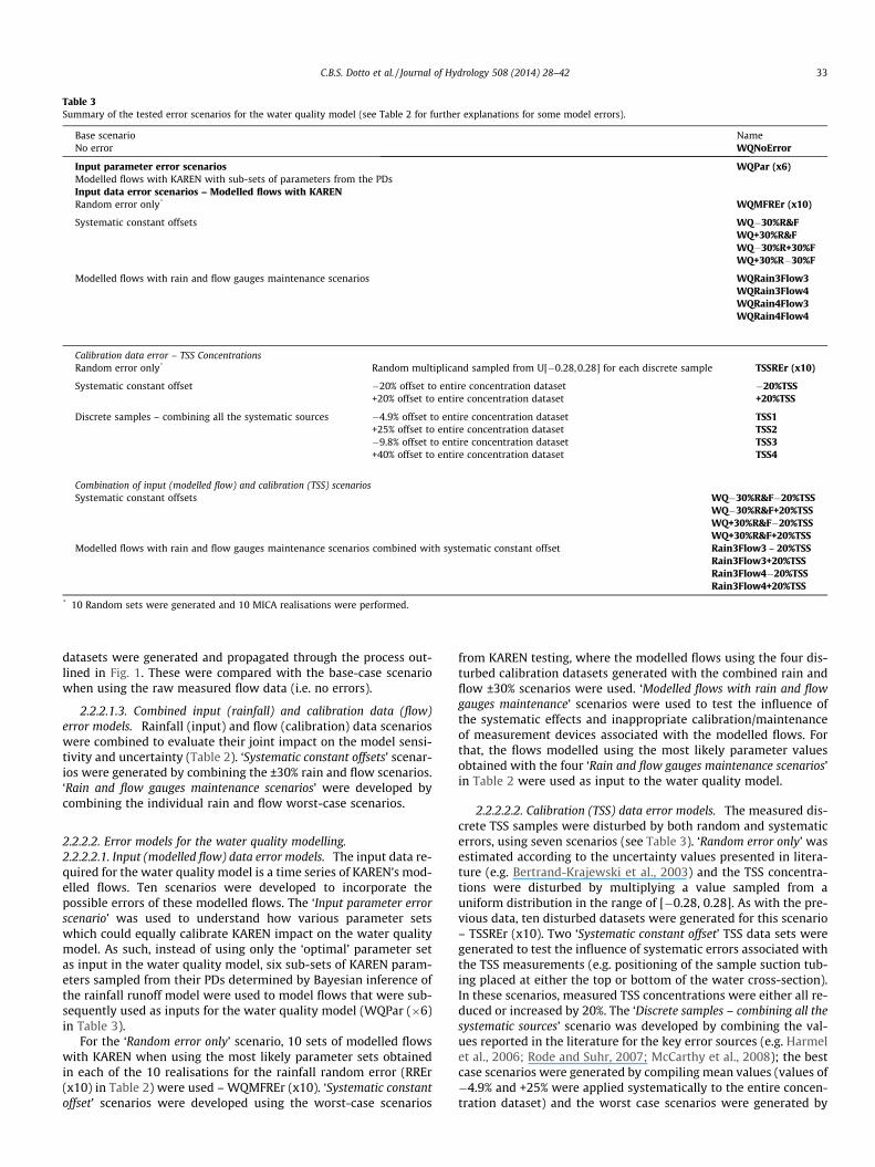
Table 3Summary of the tested error scenarios for the water quality model (see Table 2 for further explanations for some model errors).

Base scenario NameNo error WQNoError

Input parameter error scenarios WQPar (x6)Modelled flows with KAREN with sub-sets of parameters from the PDsInput data error scenarios – Modelled flows with KARENRandom error only* WQMFREr (x10)

Systematic constant offsets WQ�30%R&FWQ+30%R&FWQ�30%R+30%FWQ+30%R�30%F

Modelled flows with rain and flow gauges maintenance scenarios WQRain3Flow3WQRain3Flow4WQRain4Flow3WQRain4Flow4

Calibration data error – TSS ConcentrationsRandom error only* Random multiplicand sampled from U[�0.28,0.28] for each discrete sample TSSREr (x10)

Systematic constant offset �20% offset to entire concentration dataset �20%TSS+20% offset to entire concentration dataset +20%TSS

Discrete samples – combining all the systematic sources �4.9% offset to entire concentration dataset TSS1+25% offset to entire concentration dataset TSS2�9.8% offset to entire concentration dataset TSS3+40% offset to entire concentration dataset TSS4

Combination of input (modelled flow) and calibration (TSS) scenariosSystematic constant offsets WQ�30%R&F�20%TSS

WQ�30%R&F+20%TSSWQ+30%R&F�20%TSSWQ+30%R&F+20%TSS

Modelled flows with rain and flow gauges maintenance scenarios combined with systematic constant offset Rain3Flow3 – 20%TSSRain3Flow3+20%TSSRain3Flow4�20%TSSRain3Flow4+20%TSS

* 10 Random sets were generated and 10 MICA realisations were performed.

C.B.S. Dotto et al. / Journal of Hydrology 508 (2014) 28–42 33

datasets were generated and propagated through the process out-lined in Fig. 1. These were compared with the base-case scenariowhen using the raw measured flow data (i.e. no errors).

2.2.2.1.3. Combined input (rainfall) and calibration data (flow)error models. Rainfall (input) and flow (calibration) data scenarioswere combined to evaluate their joint impact on the model sensi-tivity and uncertainty (Table 2). ‘Systematic constant offsets’ scenar-ios were generated by combining the ±30% rain and flow scenarios.‘Rain and flow gauges maintenance scenarios’ were developed bycombining the individual rain and flow worst-case scenarios.

2.2.2.2. Error models for the water quality modelling.2.2.2.2.1. Input (modelled flow) data error models. The input data re-quired for the water quality model is a time series of KAREN’s mod-elled flows. Ten scenarios were developed to incorporate thepossible errors of these modelled flows. The ‘Input parameter errorscenario’ was used to understand how various parameter setswhich could equally calibrate KAREN impact on the water qualitymodel. As such, instead of using only the ‘optimal’ parameter setas input in the water quality model, six sub-sets of KAREN param-eters sampled from their PDs determined by Bayesian inference ofthe rainfall runoff model were used to model flows that were sub-sequently used as inputs for the water quality model (WQPar (�6)in Table 3).

For the ‘Random error only’ scenario, 10 sets of modelled flowswith KAREN when using the most likely parameter sets obtainedin each of the 10 realisations for the rainfall random error (RREr(x10) in Table 2) were used – WQMFREr (x10). ‘Systematic constantoffset’ scenarios were developed using the worst-case scenarios

from KAREN testing, where the modelled flows using the four dis-turbed calibration datasets generated with the combined rain andflow ±30% scenarios were used. ‘Modelled flows with rain and flowgauges maintenance’ scenarios were used to test the influence ofthe systematic effects and inappropriate calibration/maintenanceof measurement devices associated with the modelled flows. Forthat, the flows modelled using the most likely parameter valuesobtained with the four ‘Rain and flow gauges maintenance scenarios’in Table 2 were used as input to the water quality model.

2.2.2.2.2. Calibration (TSS) data error models. The measured dis-crete TSS samples were disturbed by both random and systematicerrors, using seven scenarios (see Table 3). ‘Random error only’ wasestimated according to the uncertainty values presented in litera-ture (e.g. Bertrand-Krajewski et al., 2003) and the TSS concentra-tions were disturbed by multiplying a value sampled from auniform distribution in the range of [�0.28, 0.28]. As with the pre-vious data, ten disturbed datasets were generated for this scenario– TSSREr (x10). Two ‘Systematic constant offset’ TSS data sets weregenerated to test the influence of systematic errors associated withthe TSS measurements (e.g. positioning of the sample suction tub-ing placed at either the top or bottom of the water cross-section).In these scenarios, measured TSS concentrations were either all re-duced or increased by 20%. The ‘Discrete samples – combining all thesystematic sources’ scenario was developed by combining the val-ues reported in the literature for the key error sources (e.g. Harmelet al., 2006; Rode and Suhr, 2007; McCarthy et al., 2008); the bestcase scenarios were generated by compiling mean values (values of�4.9% and +25% were applied systematically to the entire concen-tration dataset) and the worst case scenarios were generated by

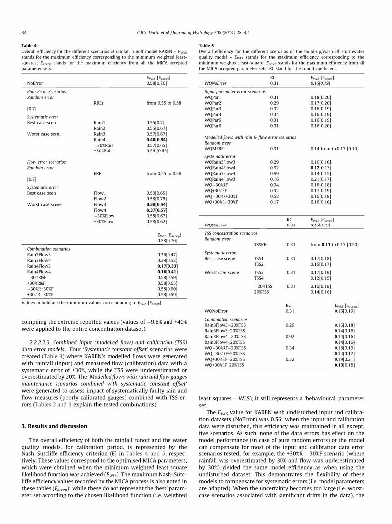
Table 4Overall efficiency for the different scenarios of rainfall runoff model KAREN – EWLS

stands for the maximum efficiency corresponding to the minimum weighted least-squares; Eaccep stands for the maximum efficiency from all the MICA acceptedparameter sets.

EWLS [Eaccep]NoError 0.58[0.76]

Rain Error ScenariosRandom error

RREr from 0.55 to 0.58[0.7]

Systematic errorBest case scen. Rain1 0.55[0.7]

Rain2 0.55[0.67]Worst case scen. Rain3 0.57[0.67]

Rain4 0.40[0.54]�30%Rain 0.57[0.65]+30%Rain 0.56 [0.65]

Flow error scenariosRandom error

FREr from 0.55 to 0.58[0.7]

Systematic errorBest case scen. Flow1 0.50[0.65]

Flow2 0.58[0.75]Worst case scene Flow3 0.38[0.54]

Flow4 0.37[0.57]�30%Flow 0.58[0.67]+30%Flow 0.58[0.62]

EWLS [Eaccep]0.58[0.76]

Combination scenariosRain3Flow3 0.36[0.47]Rain3Flow4 0.39[0.52]Rain4Flow3 0.17[0.33]Rain4Flow4 0.16[0.41]�30%R&F 0.58[0.59]+30%R&F 0.58[0.65]�30%R+30%F 0.58[0.60]+30%R�30%F 0.58[0.59]

Values in bold are the minimum values corresponding to EWLS [Eaccep]

Table 5Overall efficiency for the different scenarios of the build-up/wash-off stormwaterquality model – EWLS stands for the maximum efficiency corresponding to theminimum weighted least-square; Eaccep stands for the maximum efficiency from allthe MICA accepted parameter sets; RC stand for the runoff coefficient.

RC EWLS [Eaccep]WQNoError 0.31 0.16[0.19]

Input parameter error scenariosWQPar1 0.31 0.18[0.20]WQPar2 0.29 0.17[0.20]WQPar3 0.32 0.16[0.19]WQPar4 0.34 0.16[0.19]WQPar5 0.31 0.16[0.19]WQPar6 0.31 0.16[0.20]

Modelled flows with rain & flow error scenariosRandom errorWQMFREr 0.31 0.14 from to 0.17 [0.19]

Systematic errorWQRain3Flow3 0.29 0.16[0.16]WQRain4Flow4 0.92 0.12[0.13]WQRain3Flow4 0.99 0.14[0.15]WQRain4Flow3 0.16 0.21[0.17]WQ�30%RF 0.34 0.16[0.18]WQ+30%RF 0.32 0.17[0.19]WQ�30%R+30%F 0.58 0.16[0.18]WQ+30%R�30%F 0.17 0.16[0.16]

RC EWLS [Eaccep]WQNoError 0.31 0.16[0.19]

TSS concentration scenariosRandom error

TSSREr 0.31 from 0.11 to 0.17 [0.20]

Systematic errorBest case scene TSS1 0.31 0.17[0.18]

TSS2 0.15[0.17]

Worst case scene TSS3 0.31 0.17[0.19]TSS4 0.12[0.15]

�20%TSS 0.31 0.16[0.19]20%TSS 0.14[0.16]

RC EWLS [Eaccep]WQNoError 0.31 0.16[0.19]

Combination scenariosRain3Flow3�20%TSS 0.29 0.16[0.18]Rain3Flow3+20%TSS 0.14[0.16]Rain3Flow4�20%TSS 0.92 0.14[0.16]Rain3Flow4+20%TSS 0.14[0.16]WQ�30%RF�20%TSS 0.34 0.18[0.19]WQ�30%RF+20%TSS 0.14[0.17]WQ+30%RF�20%TSS 0.32 0.19[0.21]WQ+30%RF+20%TSS 0.13[0.15]

34 C.B.S. Dotto et al. / Journal of Hydrology 508 (2014) 28–42

compiling the extreme reported values (values of �9.8% and +40%were applied to the entire concentration dataset).

2.2.2.2.3. Combined input (modelled flow) and calibration (TSS)data error models. Four ‘Systematic constant offset’ scenarios werecreated (Table 3) where KAREN’s modelled flows were generatedwith rainfall (input) and measured flow (calibration) data with asystematic error of ±30%, while the TSS were underestimated oroverestimated by 20%. The ‘Modelled flows with rain and flow gaugesmaintenance scenarios combined with systematic constant offset’were generated to assess impact of systematically faulty rain andflow measures (poorly calibrated gauges) combined with TSS er-rors (Tables 2 and 3 explain the tested combinations).

3. Results and discussion

The overall efficiency of both the rainfall runoff and the waterquality models, for calibration period, is represented by theNash–Sutcliffe efficiency criterion (E) in Tables 4 and 5, respec-tively. These values correspond to the optimised MICA parameters,which were obtained when the minimum weighted least-squarelikelihood function was achieved (EWLS). The maximum Nash–Sutc-liffe efficiency values recorded by the MICA process is also noted inthese tables (Eaccep); while these do not represent the ‘best’ param-eter set according to the chosen likelihood function (i.e. weighted

least squares – WLS), it still represents a ‘behavioural’ parameterset.

The EWLS value for KAREN with undisturbed input and calibra-tion datasets (NoError) was 0.56; when the input and calibrationdata were disturbed, this efficiency was maintained in all except,five scenarios. As such, none of the data errors has effect on themodel performance (in case of pure random errors) or the modelcan compensate for most of the input and calibration data errorscenarios tested; for example, the +30%R � 30%F scenario (whererainfall was overestimated by 30% and flow was underestimatedby 30%) yielded the same model efficiency as when using theundisturbed dataset. This demonstrates the flexibility of thesemodels to compensate for systematic errors (i.e. model parametersare adapted). When the uncertainty becomes too large (i.e. worst-case scenarios associated with significant drifts in the data), the

C.B.S. Dotto et al. / Journal of Hydrology 508 (2014) 28–42 35

calibration procedure is no longer able to compensate hence pro-ducing significantly lower E values; e.g. for the Rain4Flow4 combi-nation scenario (Table 2) which does not only contain a constantsystematic error but also a growing error between maintenanceintervals which cannot be compensated by parameter adaption.

The EWLS for the build-up wash-off model were consistentlylow, independent of whether or not the input or calibration datawere disturbed. With undisturbed input and calibration datasets(WQNoError) a value of 0.16 was achieved, while for the differenterror models, EWLS varies between 0.11 and 0.21. These low valuesmight reflect structural errors in the model, which limits the mod-el’s performance and constrains to significantly distinguish be-tween impacts of the different error models (especially as theresults are based on a random MCMC process). However, the low-est EWLS values are still identified in that three scenarios again rep-resenting worst-case situations where the model is no longer ableto compensate for large measurement errors.

The overall model efficiency varied in the validation data period(data not shown). Considering the NoError scenario, the Nash–Sutcliffe efficiency obtained with the parameter set correspondingto the minimum weighted least-square likelihood function (in thecalibration period – EWLS) dropped from 0.58 in the calibration to0.52 in the validation. This could be explained by (1) the fact thatthe validation data period was much drier than the calibration dataperiod and (2) that the model was calibrated using a least squareslikelihood function, which meant that the model was not well ad-justed for the prediction of the lower flows seen in the validationdata period (please refer to Dotto el al, 2011 for further discussion).An example of a more drastic drop was found for the �30%R+30%Fscenario, in which the same efficiency measure dropped from 0.58to 0.1. This drastic drop can be explained by the fact the model thatwas calibrated to deal with a much higher amount of runoff(in�30%R+30%F). This is reflected by the range of parameter valuesthat calibrated the model for this scenario (e.g. mean EIF valuechanged from around 30% in the NoError to 60% in �30%R+30%Fscenario). As such, the model was not able to predict the ‘normal’flow levels observed during the validation period. The oppositewas observed for the Rain4 scenario, in which the Nash–Sutcliffeincreased from 0.4 to 0.5. In this case the calibrated parameter val-ues were tuned to calibrate the model for higher rainfall rates thannormal, and therefore the model was able to better predict the‘normal’ flow levels to the validation (which are mostly lower thanthe calibration period).

Fig. 2. Histograms for KAREN parameters (top) obtained from the ‘NoError’ scenario andand histograms for the build-up/wash-off model parameters (bottom) obtained from the ‘– TSSREr (x10) (see Table 2 for abbreviations).

3.1. Parameter sensitivity

The results, for both rainfall runoff and water quality models,are presented according to the impact of the error types (i.e. No er-ror, Random error and Systematic error) on each of the calibrationparameters of the two models. For each error type, we start by dis-cussing the impacts of input data errors, then calibration data er-rors, and finish by discussing the impacts of the jointpropagation of input and calibration data errors.

3.1.1. No error analysisThe PDs of parameters revealed that KAREN is quite sensitive to

the effective EIF, TOC and eV, while less influenced by li (see Fig. 2),which is in line with previous studies (Dotto et al., 2012). Thebuild-up/wash-off model is sensitive to M0, k2, k3 and r, but notvery influenced by k1. In addition, it was verified that M0 and k2

are very correlated mainly due to the model structure arrangementas previously described by Kanso et al. (2003).

3.1.2. Random error impact in input and calibration data3.1.2.1. Rainfall runoff model – KAREN. Random errors in measuredinput and calibration data did not significantly impact on the mod-el’s performance (Tables 4 and 5) and sensitivity. For example, EWLS

ranged from 0.55 to 0.58 for the 10 sets of data generated withKAREN rainfall random errors. The PDs of KAREN parameters forthe rainfall random errors scenario have very similar shape asthose for the ‘NoError’ scenario (Fig. 2, top). The same was ob-served when disturbing the rainfall input for spatial distributionerrors (RainSD) and the flow data for random errors in measure-ments (FREr). While Kleidorfer et al. (2009) propagated the randominput data errors in the same stormwater model in a slightly differ-ent way, the conclusion, that random errors do not represent a ma-jor impact in the model sensitivity, was the same. For this reason,the random errors in both input and calibration data were not as-sessed further (i.e. were not combined with the systematic errors).

3.1.2.2. Water quality model – Build-up/wash-off. Similarly, thebuild-up wash-off model PDs were unchanged when applying ran-dom errors to the input and calibration data (Fig. 2, bottom). Again,Kleidorfer et al. (2009) found similar results when analysing TSSand TN loads with a simple regression equation. As such, theseerrors were not combined with the systematic errors.

from the 10 sets of data generated with KAREN rainfall random errors – RREr (x10);WQNoError’ scenario and from the 10 sets of data generated with TSS random errors

Table 6Rainfall runoff model KAREN – Histograms of parameter PDs for the different error scenarios. The variation in the x-axis is to facilitate thevisualisation of specific scenarios.

ScenariosNoerror

EIF (%) TOC (min) li (mm) ev (mm/day)

-30%Rain+30%Rain

20 40 600

40

90 1100

40

1 2.5 4.50

40

0 0.125 0.250

40

-30%Flow+30%Flow

20 40 600

40

90 1100

40

1 2.5 4.50

40

0 0.125 0.250

40

-30%R+30%F+30%R-30%F

20 40 600

40

90 1100

40

1 2.5 4.50

40

0 0.125 0.250

40

-30%R&F+30%R&F

20 40 600

40

90 1100

40

1 2.5 4.50

40

0 0.125 0.250

40

Rain1Rain2d 3

20 40 600

40

90 1100

40

1 2.5 4.50

40

0 0.125 0.250

40

Rain3Rain4

20 40 600

40

90 1100

40

1 2.5 4.50

40

0 0.125 0.250

40

Flow1Flow2

20 40 600

40

90 1100

40

1 2.5 4.50

40

0 0.125 0.250

40

Flow3Flow4

95 990

40

20300

40

162 168

40

90 110

40

1 2.5 4.50

40

0 0.125 0.250

40

Rain3Flow3Rain3Flow4

20300

40

95 990

40

162 168

40

90 110

40

1 2.5 4.50

40

0 0.125 0.250

40

Rain4Flow3Rain4Flow4

92 980

40

20300

40

162 168

40

80 110

40

1 2.5 4.50

40

0 0.125 0.250

40

36 C.B.S. Dotto et al. / Journal of Hydrology 508 (2014) 28–42

Fig. 2 Histograms for KAREN parameters (top) obtained fromthe ‘NoError’ scenario and from the 10 sets of data generated withKAREN rainfall random errors – RREr (x10); and histograms for thebuild-up/wash-off model parameters (bottom) obtained from the‘WQNoError’ scenario and from the 10 sets of data generated withTSS random errors – TSSREr (x10) (see Table 2 for abbreviations).

3.1.3. Systematic errors in input and calibration data3.1.3.1. Rainfall runoff model – KAREN. Impact of systematic errorson parameter sensitivity (visualised in the parameter distribution)

is shown in Table 6. When rainfall is systematically overestimated(e.g.+30%Rain), or flow is underestimated (e.g. �30%Flow), EIF de-creases (to compensate for these errors). These shifts were eithercompensated or accentuated when combining these rainfall andflow errors; for example, in the �30%R+30%F and +30%R�30%F sce-narios, pronounced shifts in EIF were observed, while in the�30%R&F and +30%R&F scenarios little differences were seen inthe PDs as compared with the ‘NoError’ scenario. These results re-flect the ability of the model parameter EIF to entirely compensatefor systematic errors found in the measured datasets and shows

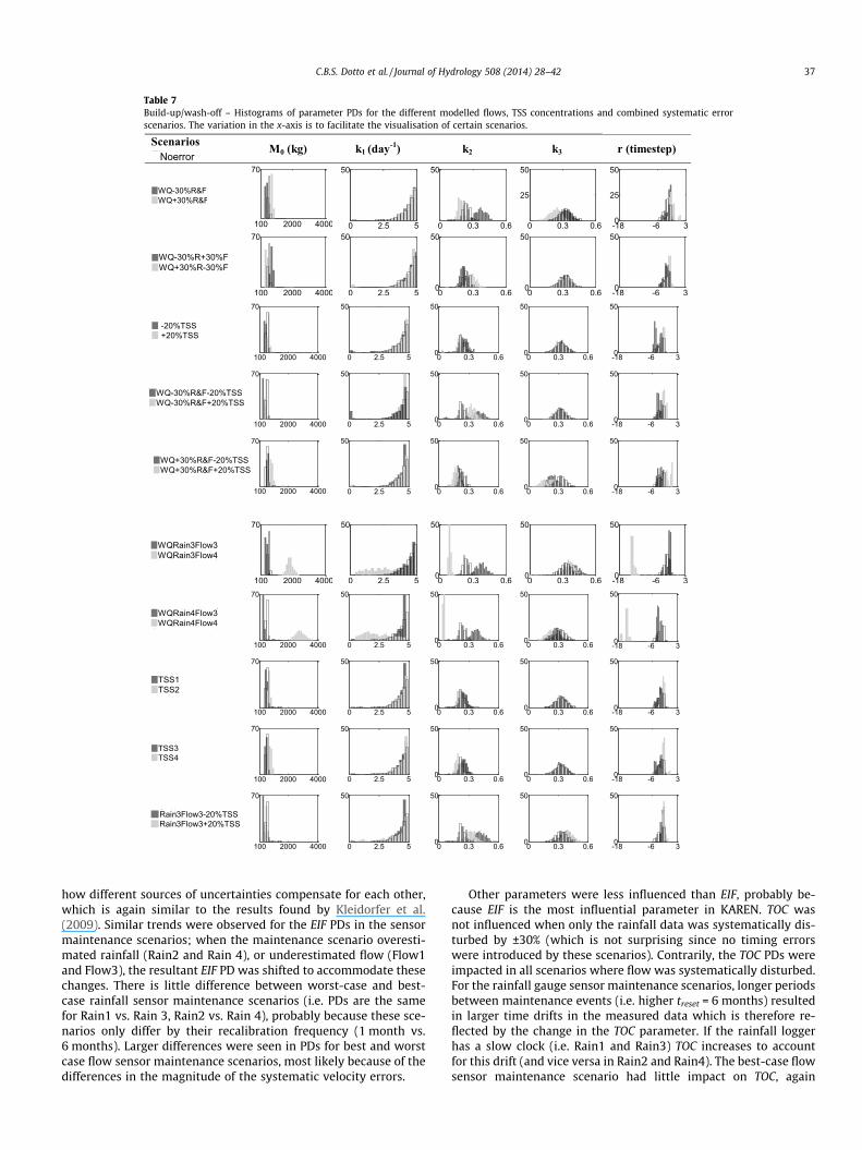
Table 7Build-up/wash-off – Histograms of parameter PDs for the different modelled flows, TSS concentrations and combined systematic errorscenarios. The variation in the x-axis is to facilitate the visualisation of certain scenarios.

ScenariosNoerror

M0 (kg) k1 (day-1) k2 k3 r (timestep)

WQ-30%R&FWQ+30%R&F

100 2000 4000

70

0 2.5 5

50

0 0.3 0.6

50

0 0.3 0.6

25

50

-18 -6 30

25

50

WQ-30%R+30%FWQ+30%R-30%F

100 2000

70

4000 0 2.5 5

50

0 0.3 0.60

50

0 0.3 0.60

50

-18 -6 30

50

-20%TSS +20%TSS

100 2000 4000

70

0 2.5 5

50

0 0.3 0.60

50

0 0.3 0.60

50

-18 -6 30

50

70WQ-30%R&F-20%TSSWQ-30%R&F+20%TSS

100 2000 4000

70

0 2.5 5

50

0 0.3 0.60

50

0 0.3 0.60

50

-18 -6 30

50

70WQ+30%R&F-20%TSSWQ+30%R&F+20%TSS

100 2000 4000

70

0 2.5 5

50

0 0.3 0.60

50

0 0.3 0.60

50

-18 -6 30

50

100 2000 4000

70

0 2.5 5

50

0 0.3 0.60

50

0 0.3 0.60

50

-18 -6 30

50

WQRain4Flow3WQRain4Flow4

100 2000 4000

70

0 2.5 5

50

0 0.3 0.60

50

0 0.3 0.60

50

-18 -6 30

50

TSS1TSS2

100 2000 4000

70

0 2.5 5

50

0 0.3 0.60

50

0 0.3 0.60

50

-18 -6 30

50

TSS3TSS4

100 2000 4000

70

0 2.5 5

50

0 0.3 0.60

50

0 0.3 0.60

50

-18 -6 30

50

Rain3Flow3-20%TSSRain3Flow3+20%TSS

100 2000 4000

70

0 2.5 5

50

0 0.3 0.60

50

0 0.3 0.60

50

-18 -6 30

50

WQRain3Flow3WQRain3Flow4

C.B.S. Dotto et al. / Journal of Hydrology 508 (2014) 28–42 37

how different sources of uncertainties compensate for each other,which is again similar to the results found by Kleidorfer et al.(2009). Similar trends were observed for the EIF PDs in the sensormaintenance scenarios; when the maintenance scenario overesti-mated rainfall (Rain2 and Rain 4), or underestimated flow (Flow1and Flow3), the resultant EIF PD was shifted to accommodate thesechanges. There is little difference between worst-case and best-case rainfall sensor maintenance scenarios (i.e. PDs are the samefor Rain1 vs. Rain 3, Rain2 vs. Rain 4), probably because these sce-narios only differ by their recalibration frequency (1 month vs.6 months). Larger differences were seen in PDs for best and worstcase flow sensor maintenance scenarios, most likely because of thedifferences in the magnitude of the systematic velocity errors.

Other parameters were less influenced than EIF, probably be-cause EIF is the most influential parameter in KAREN. TOC wasnot influenced when only the rainfall data was systematically dis-turbed by ±30% (which is not surprising since no timing errorswere introduced by these scenarios). Contrarily, the TOC PDs wereimpacted in all scenarios where flow was systematically disturbed.For the rainfall gauge sensor maintenance scenarios, longer periodsbetween maintenance events (i.e. higher treset = 6 months) resultedin larger time drifts in the measured data which is therefore re-flected by the change in the TOC parameter. If the rainfall loggerhas a slow clock (i.e. Rain1 and Rain3) TOC increases to accountfor this drift (and vice versa in Rain2 and Rain4). The best-case flowsensor maintenance scenario had little impact on TOC, again

38 C.B.S. Dotto et al. / Journal of Hydrology 508 (2014) 28–42

because timing issues were not introduced. The worst-case flowsensor maintenance scenarios did impact TOC, probably becausethe incremental error added/subtracted to/from the level measure-ments altered the measured hydrographs which changed the prob-ability distribution of TOC. When both input and calibrationdatasets were systematically disturbed, the resulting PDs are sim-ilar to the ones obtained for the flow scenarios.

The initial loss (li) reveals PDs that are distributed among real-istic values for this parameter (i.e. values between 0.5 and 2 mmare usually adopted in similar urban storm models; (e.g. Chiewand McMahon, 1999). Introducing systematic errors into the rain-fall data (i.e. ±30%Rain) slightly influenced the li PDs, while system-atic flow errors (i.e. ±30%Flow) seemed to have no observableinfluence. When both rainfall and flow datasets were systemati-cally disturbed simultaneously (i.e. ±30%R&F, �30%R+30%F and+30%R�30%F), the resultant li PDs resembled those of the rainfallonly scenarios. Similar results were found when testing variousmaintenance scenarios; overestimated rainfall led to higher li val-ues and vice versa for both best and worst case scenarios. Whilethe best-case flow sensor maintenance scenarios (Flow1 andFlow2) yielded no effect on PDs of li, the worst-case scenarios,including the combined input and calibration data errors (e.g.Rain4Flow4) significantly impacted them. It is hypothesised thatthese results are directly linked to EIF’s behaviour, which compen-sated for the dramatic increase in flow measurements in Flow4 andits related scenarios; indeed, it is common to see a relationship be-tween EIF and li, as they are intrinsically linked in the model struc-ture (Boyd et al., 1993).

The eV parameter reflected some of the model limitations.While common values for evaporation in Melbourne are around4 mm/day, the parameter PDs were in the range of 0.01 and0.15 mm/day for most of the scenarios. This parameter is used todrain li (modelled as a reservoir) during dry weather (i.e. betweenevents). So it cannot compensate for changes in rainfall intensity orflow rate. For example a li of 1.5 mm is drained over 10 days wheneV is assumed to be 0.15 mm/day. The realistic (physical) value of4 mm/day could only be identified in the model when very shortdry weather periods between rainfall events exit (i.e. about0.25 days). As length of rainfall events or dry weather periods werenot affected by any of the error scenarios hardly a change in PD canbe seen. (In general the shape of eV PDs, and most likely values, didnot change much within the various scenarios.

In summary, the results from this sensitivity analysis showedthat the systematic errors in input and calibration data (individualor combined) influenced most of the parameters’ distributions. Italso demonstrated that the parameters were able to compensatefor most of the scenarios, mainly for the best case ones. The factthat the model parameters’ compensate for most rainfall errorswas also found by Younger et al. (2009) when evaluating the im-pact of rainfall data error in a hydrologic rainfall runoff model.They found that while the peak flows changed significantly forthe different scenarios, the model performance did not. Further-more, the propagation of input and calibration data errors providednew information about the model structure and its parameters.

Fig. 3. Histograms for the build-up/wash-off model parameters obtained with the inparameters from the PDs – WQPar (x6).

3.1.3.2. Water quality model – Build-up/wash-off. The. impact of sys-tematic errors on parameter sensitivity is shown in Table 7. Resultsfrom the input data error scenarios showed that M0 is directlylinked to the runoff volume; its PDs shifted towards higher valuesin all input data error scenarios where modelled flows were over-estimated (WQ+30%R&F WQ�30%R+30%F, WQRain3Flow4 andWQRain4Flow4) and towards lower values when modelled flowswere underestimated (�30%R&F WQ+30%R�30%F, WQRain3Flow3and WQRain4Flow3). Similarly, M0 was sensitive to calibrationdata error, and varied according to the increase (or decrease) inthe TSS concentrations for each scenario. The impact of combinedinput and calibration data errors on M0 parameter indicated a clear‘additive’ effect for different sources of uncertainties. For example,the combined increase in both volumes and TSS concentration(WQ+30%RF+20%TSS) shifted M0 for the 10% difference as the mod-el does not need to compensate for the +20% in both data. Follow-ing the same pattern, M0 shifts the most when the volumes areincreased and TSS decreased (WQ+30%RF�20%TSS).

The PDs for the k1 parameter were skewed towards the upperlimit of the parameter value (i.e. 5 day�1) for most of the scenarios,which reflects the modelling boundary conditions (i.e. modelstructure limitation). However, testing conducted with MICA con-firmed that this parameter will always skew toward the upperbound of its boundary condition (data not shown). As values ofk1 higher than 5 day�1 are unrealistic (i.e. quick build-up of masson the surface), 5 was still used as the upper bound. These resultssuggest that the build-up of TSS occurs extremely quickly, whichconfirms that the wash-off during typical rainfall events removeonly a very small portion of solids accumulated in the surface(e.g. Vaze and Chiew, 2003). Results from the scenarios whereFlow4 was included were different; i.e. the model was insensitiveto k1 indicating that the errors were compensated by the otherparameters and mainly Mo (as Mo is correlated with k1). It ishypothesised that these results would be different if other pollu-tants were being modelled, for example the antecedent conditionsin the catchment influences the amount of pathogens available onthe surface (McCarthy et al., 2011).

Results from the individual input and calibration data error sce-narios, and also from the combined error scenarios indicated thatthe peaks in the PDs of k2 shifted to the opposite direction of shiftin M0 PDs. Again, the high correlation between these two parame-ters is illustrated. Moreover, the model sensitivity to k2 (Table 7)confirms the wash-off variability within the event, as largeramounts of TSS are washed in the beginning of the event.

PDs of k3 varied with the input data scenarios and did notchange at all for the calibration data error scenarios. This is be-cause the k3 parameter is linked to the input data in Eq. (2). Besidesk3 only responds to changes in variability of the data; this meansthat only scaling the input or output data (constant offset scenar-ios) does not impact on this parameter. In fact, this wash-off expo-nent is related to the kinetic energy of the rainfall, representedhere using the modelled effective runoff rates, in mm/hr, fromimpervious areas. k3 ranges from 0.25 in WQ+30%RF andWQRain4Flow4 to 0.42 in Rain3Flow3+20%TSS, which is in

put parameter error scenarios; i.e. ‘Modelled flows with KAREN with sub-sets of

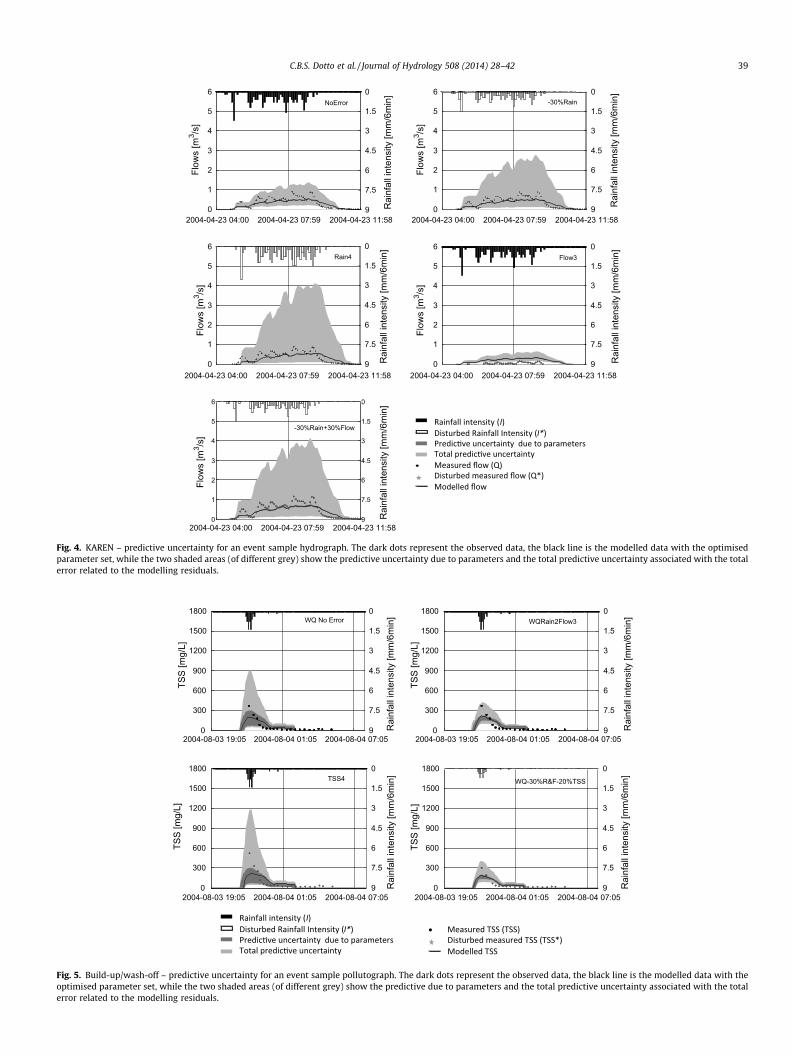
Fig. 4. KAREN – predictive uncertainty for an event sample hydrograph. The dark dots represent the observed data, the black line is the modelled data with the optimisedparameter set, while the two shaded areas (of different grey) show the predictive uncertainty due to parameters and the total predictive uncertainty associated with the totalerror related to the modelling residuals.

Fig. 5. Build-up/wash-off – predictive uncertainty for an event sample pollutograph. The dark dots represent the observed data, the black line is the modelled data with theoptimised parameter set, while the two shaded areas (of different grey) show the predictive due to parameters and the total predictive uncertainty associated with the totalerror related to the modelling residuals.

C.B.S. Dotto et al. / Journal of Hydrology 508 (2014) 28–42 39

Table 8Summary of the observations within the uncertainty bounds for sample scenarios (validation period results for the rainfall runoff model are given between brackets).

Rainfall runoff KAREN

NoError �30%Rain Rain4 Flow3 �30%R+30%F

Observations within the parameter uncertainty bound (%) 9 [8] 9 [1] 6 [2] 20 [2] 9 [2]Observations within the total uncertainty bound (%) 63 [30] 87 [98] 91 [30] 59 [30] 84 [100]

Build-up/Wash-off

WQNoError WQRain3Flow3 TSS4 WQ�30%RF+20%TSS

Observations within the parameter uncertainty bound (%) 48 15 53 19Observations within the total uncertainty bound (%) 72 40 79 42

Fig. 6. KAREN – predictive uncertainty for an event sample hydrograph for the validation data period. The dark dots represent the observed data during the validation period(non-biased), the black line is the modelled data with the optimised parameter set for the specific scenarios, while the two shaded area (of different grey) shows the totalpredictive uncertainty associated with the total error related to the modelling residuals.

40 C.B.S. Dotto et al. / Journal of Hydrology 508 (2014) 28–42

accordance to the 0.29 value found by McCarthy et al. (2011) forsediment transport. For the combined input and calibration dataerror scenarios, k3 only ranged for the scenarios in which the vol-umes were overestimated (e.g. WQ+30%RF�20%TSS andWQ+30%RF+20%TSS).

While the change in the translation parameter r was not signif-icant for most of the input, calibration and combined error scenar-ios, it was extreme for the specific cases in which the flow worstcase scenario in the rainfall runoff model was included (input dataerror: WQRain3Flow4 and WQRain4Flow4; combined data error:WQRain3Flow4±20%TSS). These major shifts are due to the factthat Flow4 was the scenario that implied the worst ‘Flow gaugemaintenance scenario’. The 6 months period for re-calibration of

the sensor (both timing and level/velocity) significantly changedthe properties and location of the modelled hydrograph. As a con-sequence r was affected. For example, r shifted from 3 timesteps(18 min) in the ‘NoError’ scenario to more than 10 timesteps(1 h) in WQRain3Flow4 and WQRain4Flow4.

The five parameters of the build-up/wash-off model werenot significantly impacted when the flows modelled withsub-sets of parameters from KAREN PDs were used to generateTSS concentrations (Fig. 3). This might be because the PD gen-erated for the most sensitive parameter EIF in the ‘NoError’scenario was very narrow (e.g. Fig. 2), and thus different com-binations of KAREN model parameters had very little effect onthe model flows.

C.B.S. Dotto et al. / Journal of Hydrology 508 (2014) 28–42 41

In summary, the results indicated that while the sensitivity ofthe model to its parameters did not alter significantly (i.e. theshape of the parameter distributions remained the same) the mod-el parameters were able to compensate for the errors in measuredinput and calibration data (i.e. parameter values or the position ofthe distributions changed).

Table 7 Build-up/wash-off – Histograms of parameter PDs forthe different modelled flows, TSS concentrations and combinedsystematic error scenarios. The variation in the x-axis is to facilitatethe visualisation of certain scenarios.

3.2. Modelling uncertainty

Figs. 4 and 5 present the predictive uncertainty for an eventwith different error scenarios for KAREN and the build-up/wash-off model, respectively. Table 8 shows a summary of the observa-tions (corresponding to each scenario) which fall within theuncertainty bounds for example scenarios (representing some ofthe different worst case scenarios). In general, the coverage fromparameter uncertainties for KAREN was very low. This is a reflec-tion of the shape and form of the parameter distributions shownin Fig. 4; indeed, KAREN’s most influential parameters have a verynarrow distribution for most of the scenarios. This was thought tobe caused by KAREN’s limited ability to represent pervious surfaceflows and baseflow; without these processes, the model was un-able to predict these lower flows (which dominate the dataset interms of absolute number of data points) meaning that its coveragewas very low (i.e. coverage equally weights all data points in thedataset). Furthermore the fact that the number of observationswithin the parameter uncertainty bands is the same or very similarfor the ‘NoError’ scenario and the �30%Rain, Rain4 and,�30%R+30%F indicates that the effect of measured data uncertaintyis small (see Fig. 6).

The total uncertainty associated with both models varied withthe different scenarios. The percentage of observations within thetotal uncertainty bound for the build-up/wash-off model variedand was almost linearly correlated with the relative number ofobservations within the parameter uncertainty limits (Table 8).KAREN on the other hand, did not present such a clear pattern. Itseems that the total uncertainty was intrinsically related to thescenario characteristics. For example, for Flow3 scenario, whichis the worst case scenario underestimating flows, the coverage ofthe parameter uncertainty increased when compared to the ‘NoEr-ror’ scenario, while the total uncertainty decreased.

As seen in Table 8 the coverage from the total uncertainty forthe NoError scenario was lower during the validation data period,which indicates that the simple model (i.e. not based on the de-tailed physics of the urban drainage systems) is not able to extrap-olate the calibration results into the future. Similar comparison forthe other scenarios is compromised as the model was calibratedwith biased data and validation with non-biased data.

4. Conclusions

The paper presented the application of a simple approach forglobal assessment of uncertainties in urban drainage models,which propagates errors in input and calibration data and evalu-ates how they impact the model calibration performance, sensitiv-ity and predictive uncertainty. The approach was tested for acoupled urban stormwater model (a simple rainfall runoff modelcoupled with a commonly used build-up/wash-off model).

Results suggested that random errors in all input and calibra-tion data had minor impact on the model performance and sensi-tivity. Systematic errors in input and calibration data on theother hand, influenced the model sensitivity (represented by the

parameter distributions). In most of the scenarios (especially thosewhere uncertainty in input and calibration data was representedusing ‘best-case’ assumptions), the errors in measured data werefully compensated by parameter calibration. For example, whenrainfall was systematically under or overestimated, the effectiveimpervious area parameter varied systematically to compensatefor the changes in the input data. In addition the model predictiveuncertainty was also compensated in most of the cases as the num-ber of observations within the parameter uncertainty bound keptfairly constant. It should then be noted that if the model parame-ters were considered initially as reflecting reality, this representa-tion was reduced when input and calibration data errors wereconsidered. Parameters were unable to compensate only in someof the scenarios where the uncertainty in the input and calibrationdata were represented using extreme worst-case scenarios. Assuch, in these few worst case scenarios, the model performancewas reduced considerably. These cases were generally linked toscenarios in which mainly the time drifts in the battery logger de-vice and calibration of water column levels were ignored for longperiods. Results suggested that re-calibration once a month issufficient.

The fact that uncertainties were assessed in such ‘ill-posed’water quality models is one weakness of this research as the ob-tained results are likely to be compromised. However, models ofsimilar model structure are commonly used in water quality mod-elling and the combination of evaluating ‘ill-posed’ models withsuch a large dataset allowed us to confirm that the model structureis possibly the main reason for the poor performance of waterquality models, and maybe not the lack of measured data. In thiscontext, it seems that simple deterministic approaches currentlyused to model water quality could be re-considered either by tak-ing into account the stochastic nature of the pollution generationprocess or by improving the model structure with a broader under-standing of the natural processes.

References

Bertrand-Krajewski, J.L., Bardin, J.P., Mourad, M., Beranger, Y., 2003. Accounting forsensor calibration, data validation, measurement and sampling uncertainties inmonitoring urban drainage systems. Water Science and Technology 47 (2), 95–102.

Beven, K., Binley, A., 1992. The future of distributed models: Model calibration anduncertainty prediction. Hydrological Processes 6 (3), 279–298.

Beven, K.J., Smith, P.J., Freer, J.E., 2008. So just why would a modeller choose to beincoherent? Journal of Hydrology 354 (1–4), 15–32.

Box, G.E.P., Cox, D.R., 1964. An analysis of transformations. Journal of the RoyalStatistical Society 26 (2), 211–252, Series B.

Boyd, M.J., Bufill, M.C., Knee, R.M., 1993. Pervious and impervious runoff in urbancatchments. Hydrological Sciences 38 (6), 463–478.

Butts, M.B., Payne, J.T., Kristensen, M., Madsen, H., 2004. An evaluation of the impactof model structure on hydrological modelling uncertainty for streamflowsimulation. Journal of Hydrology 298 (1–4), 242–266.

Chaubey, I., Haan, C.T., Grunwald, S., Salisbury, J.M., 1999. Uncertainty in the modelparameters due to spatial variability of rainfall. Journal of Hydrology 220 (48–61).

Chiew, F.H.S., McMahon, T.A., 1999. Modelling runoff and diffuse pollution loads inurban areas. Water Science and Technology 39 (12), 214–248.

Deletic, A., Dotto, C.B.S., McCarthy, D.T., Kleidorfer, M., Freni, G., Mannina, G., Uhl,M., Henrichs, M., Fletcher, T.D., Rauch, W., Bertrand-Krajewski, J.L., Tait, S., 2012.Assessing uncertainties in urban drainage models. Physics and Chemistry of theEarth, Parts A/B/C 42–44, 3–10.

Doherty, J., 2003. Model Independent Markov Chain Monte Carlo Analysis - MICA.Watermark Numerical Computing and US EPA, US.

Doherty, J., Welter, D., 2010. A short exploration of structural noise. WaterResources Research 46, W05525, doi:10.1029/2009WR008377.

Dotto, C.B.S., Mannina, G., Kleidorfer, M., Vezzaro, L., Henrichs, M., McCarthy, D.T.,Freni, G., Rauch, W., Deletic, A., 2012. Comparison of different uncertaintytechniques in urban stormwater quantity and quality modelling. WaterResearch 46 (8), 2545–2558.

Einfalt, T., Arnbjerg-Nielsen, K., Spies, S., 2002. An enquiry into rainfall datameasurement and processing for model use in urban hydrology. Water Scienceand Technology 45 (2), 147–152.

Feyen, L., Vrugt, J.A., Nualláin, B.Ó., van der Knijff, J., De Roo, A., 2007. Parameteroptimisation and uncertainty assessment for large-scale streamflow simulationwith the LISFLOOD model. Journal of Hydrology 332 (3–4), 276–289.

42 C.B.S. Dotto et al. / Journal of Hydrology 508 (2014) 28–42

Francey, M., Fletcher, T.D., Deletic, A., Duncan, H., 2010. New insights into waterquality of urban stormwater in South Eastern Australia. Journal ofEnvironmental Engineering 136 (4), 381–390.

HACH, C., 2008. Sigma 950 Flow Meter – Instrument Manual. 2009 <http://www.hach.com/fmmimghach?/CODE%3A3314-2008-1117081%7C1>.

Harmel, R., Cooper, R., Slade, R., Haney, R., Arnold, J., 2006. Cumulative uncertaintyin measured stream flow and water quality data for small watersheds.American Society of Agricultural and Biological Engineers 49 (3), 689–701.

Haydon, S., Deletic, A., 2009. Model output uncertainty of a coupled pathogenindicator-hydrologic catchment model due to input data uncertainty.Environmental Modelling and Software 24 (3), 322–328.

Kanso, A., Gromaire, M.-C., Gaume, E., Tassin, B., Chebbo, G., 2003. Bayesianapproach for the calibration of models: application to an urban stormwaterpollution model. Water Science and Technology 47 (4), 77–84.

Kleidorfer, M., Chen, S., Dotto, C.B.S., McCarthy, D., 2012. Impact of objectivefunction choice on model parameter sensitivity. In: 9th InternationalConference on Urban Drainage Modelling, Belgrade, Serbia.

Kleidorfer, M., Deletic, A., Fletcher, T.D., Rauch, W., 2009. Impact of input datauncertainties on stormwater model parameters. Water Science and Technology60 (6), 1545–1554.

Kotlash, A.R., Chessman, B.C., 1998. Effects of water sample preservation andstorage on nitrogen and phosphorus determinations: implications for the use ofautomated sampling equipment. Water Research 32 (12), 3731–3737.

Krajewski, W.F., Villarini, G., Smith, J.A., 2010. RADAR-Rainfall Uncertainties.Bulletin of the American Meteorological Society 91 (1), 87–94.

Krzysztofowicz, R., Kelly, K., 2000. Hydrologic uncertainty processor forprobabilistic river stage forecasting. Water Resources Research 36 (11), 3265–3277.

Kuczera, G., Kavetski, D., Franks, S., Thyer, M., 2006. Towards a Bayesian total erroranalysis of conceptual rainfall-runoff models: characterising model error usingstorm-dependent parameters. Journal of Hydrology 331 (1–2), 161–177.

Kuczera, G., Parent, E., 1998. Monte Carlo assessment of parameter uncertainty inconceptual catchment models: the Metropolis algorithm. Journal of Hydrology211 (1–4), 69–85.

Leecaster, M.K., Schiff, K., Tiefenthaler, L.L., 2002. Assessment of efficient samplingdesigns for urban stormwater monitoring. Water Research 36 (6), 1556–1564.

Matott, L.S., Babendreier, J.E., Purucker, S.T., 2009. Evaluating uncertainty inintegrated environmental models: a review of concepts and tools. WaterResources Research 45 (6), W06421.

McCarthy, D.T., 2008. Modelling microorganisms in urban stormwater. CivilEngineering. Melbourne, Monash University, Australia. PhD thesis, 488.

McCarthy, D.T., Deletic, A., Mitchell, V.G., Diaper, C., 2011. Development and testingof a model for Micro-Organism Prediction in Urban Stormwater (MOPUS).Journal of Hydrology 409 (1–2), 236–247.

McCarthy, D.T., Deletic, A., Mitchell, V.G., Fletcher, T.D., Diaper, C., 2008.Uncertainties in stormwater E. coli levels. Water Research 42 (6–7), 1812–1824.

Métadier, M., Bertrand-Krajewski, J.L., 2012. Interest of Bayesian learning principlefor stormwater quality modelling based on turbidity time series. In: 9thInternational Conference on Urban Drainage Modelling, Belgrade, Serbia.

Molini, A., Lanza, L.G., Barbera, P.L., 2005a. The impact of tipping-bucket raingaugemeasurement errors on design rainfall for urban-scale applications.Hydrological Processes 19, 1073–1088.

Molini, A., Lanza, L.G., La Barbera, P., 2005b. Improving the accuracy of tipping-bucket rain records using disaggregation techniques. Atmospheric Research 77(1–4), 203–217.

Mourad, M., Bertrand-Krajewski, J.-L., Chebbo, G., 2005. Calibration and validationof multiple regression models for stormwater quality prediction: datapartitioning, effect of dataset size and characteristics. Water Science andTechnology 52 (3), 45–52.

Nash, J.E., Sutcliffe, J.V., 1970. River flow forecasting through conceptualmodels part I – a discussion of principles. Journal of Hydrology 10 (3),282–290.

Rauch, W., Kinzel, H., 2007. KAREN – User Manual, Hydro-IT GmbH, Innsbruck (inGerman).

Rauch, W., Thurner, N., Harremoes, P., 1998. Required accuracy of rainfall data forintegrated urban drainage modeling. Water Science and Technology 37 (11),81–89.

Renard, B., Kuczera, G., Kavetski, D., Thyer, M., Franks, S., 2008. Bayesian Total ErrorAnalysis for Hydrologic Models: Quantifying Uncertainties Arising from Input,Output and Structural Errors. Water Down Under 2008. Engineers Australia,Modbury, SA, Causal Productions.

Rode, M., Suhr, U., 2007. Uncertainties in selected river quality data. Hydrology andEarth System Sciences 11, 863–874.

Sartor, J.D., Boyd, G.B., 1972. Water Pollution Aspects of Street SurfaceContaminants. Rep. EPA-R2-72-081. Washington, D.C., U.S. Environ. Prot.Agency.

Sevruk, B., 1982. Methods of correction for systematic error in point precipitationmeasurement for operational use. WMO Operational Hydrology Report 21 21(589), 91.

Sevruk, B., 2002. WMO questionnaire on recording precipitation gauges: state-of-the-art. Water Science and Technology 45 (2), 139–145.

Sherman, L.K., 1932. Stream-flow from Rainfall by the Unit-Graph Method.Engineering News-Record 108, 501–505.

Simic, M., Maksimovic, C., 1994. Effect of the siphon control on the dynamiccharacteristics of a tipping bucket raingauge. Hydrological Sciences 39 (1), 35–46.

Taylor, B.N., Kuyatt, C.E., 1994. Guidelines for Evaluating and Expressing theUncertainty of NIST Measurement Results. USA, NIST Technical Note 1297,National Institute of Standards and Technology.

Thyer, M., Renard, B., Kavetski, D., Kuczera, G., Franks, S.W., Srikanthan, S., 2009.Critical evaluation of parameter consistency and predictive uncertainty inhydrological modeling: a case study using Bayesian total error analysis. WaterResources Research 45, W00B14, doi:10.1029/2008WR006825.

USEPA, 2007. Storm Water Management Model (SWMM) – User Manual Version5.0. US Environmental Protection Agency (USEPA). US Environmental ProtectionAgency – EPA/600/R-05/039. Washington DC.

Vaze, J., Chiew, F.H.S., 2003. Comparative evaluation of urban storm water qualitymodels. Water Resources Research 39 (10), 1280.

Vrugt, J.A., Braak, C.J.F.t., Diks, C.G.H., Robinson, B.A., Hyman, J.M., Higdon, D., 2009.Accelerating Markov Chain Monte Carlo simulation by differential evolutionwith self-adaptive randomized subspace sampling. International Journal ofNonlinear Sciences and Numerical Simulation 10 (3), 271–288.

Yang, J., Reichert, P., Abbaspour, K.C., Xia, J., Yang, H., 2008. Comparing uncertaintyanalysis techniques for a SWAT application to the Chaohe Basin in China.Journal of Hydrology 358 (1–2), 1–23.

Younger, P.M., Freer, J.E., Beven, K.J., 2009. Detecting the effects of spatial variabilityof rainfall on hydrological modelling within an uncertainty analysis framework.Hydrological Processes 23 (14), 1988–2003.