Impact of the Anti-Aliasing Pre-Filtering on the ...

Impact of the Anti-Aliasing Pre-Filteringon the Measurement of Maximum Time Interval Error

Stefano Bregni*, Franco Setti**

*CEFRIEL, Via Fucini 2, 20133 Milano MI, ITALY, e-mail: [email protected], WWW: http://www.cefriel.it/~bregni**Politecnico di Milano, Dipartimento di Elettronica, Milano, ITALY

Abstract 2. Definition of MTIELatest ETSI and ITU-T standards recommend to evaluate MTIE

basing on Time Error data measured, for observation intervals in therange from 0.1 s to 1000 s, "through an equivalent 10 Hz, first-order,low-pass measurement filter". In this paper, the impact of such pre-filtering is thoroughly studied by simulating periodical and power-lawnoise types. Moreover, some results of measurements on telecommuni-cations clocks are provided in order to support the conclusions stem-ming from simulation with experimental evidence. The results shownpoint out that the impact that such anti-aliasing pre-filtering can havein practice may be substantial and even misleading: measurementsaccomplished through such filter may produce too optimistic results,hiding the true amplitude of phase fluctuations at timing interfaces.

A thorough treatment of MTIE and of its properties can be found in[9]. A further specific analysis is reported in [10]. Here, solely the maindefinitions are summarized for the sake of understanding and to providethe reader with the background concepts.

A general expression describing a pseudo-periodic waveform whichmodels the timing signal s(t) at the clock output is given by [11][13]

s t A t( ) sin ( )= Φ (1)where A is the peak amplitude and Φ(t) is the total instantaneous phase,expressing the ideal linear phase increasing with t and any frequencydrift or random phase fluctuation.

The generated Time function T(t) of a clock is defined, in terms ofits total instantaneous phase, as

1. Introduction Tnom

( )( )

tt= Φ

2πν(2)

major topic of discussion in standard bodies dealing with networksynchronization [1]-[3] is clock noise characterization and meas-A where νnom represents the oscillator nominal frequency. It is

worthwhile noticing that for an ideal clock Tid(t)=t holds, as expected.For a given clock, the Time Error function TE(t) (in standards alsocalled x(t) ) between its time T(t) and a reference time Tref(t) is definedas

urement. Among the quantities considered in latest international stan-dards for specification of phase and frequency stability requirements[4][5], the Maximum Time Interval Error (MTIE) has played histori-cally a major role for characterizing time and frequency performance indigital telecommunications networks [4]−[8], as specifications in termsof MTIE are well suited to support the design of equipment buffer size.

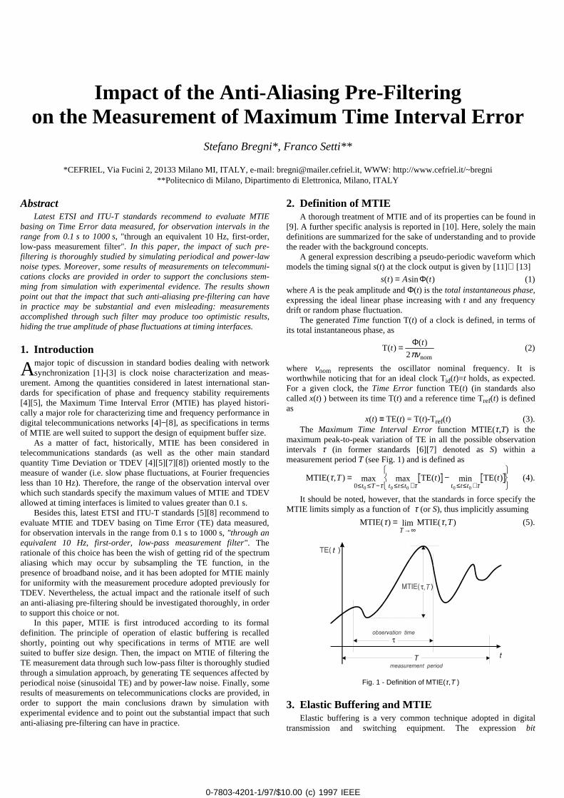
x(t) ≡ TE(t) = T(t)-Tref(t) (3).The Maximum Time Interval Error function MTIE(τ,T) is the

maximum peak-to-peak variation of TE in all the possible observationintervals τ (in former standards [6][7] denoted as S) within ameasurement period T (see Fig. 1) and is defined as

As a matter of fact, historically, MTIE has been considered intelecommunications standards (as well as the other main standardquantity Time Deviation or TDEV [4][5][7][8]) oriented mostly to themeasure of wander (i.e. slow phase fluctuations, at Fourier frequenciesless than 10 Hz). Therefore, the range of the observation interval overwhich such standards specify the maximum values of MTIE and TDEVallowed at timing interfaces is limited to values greater than 0.1 s.

MTIE TE( ) TE( )( , ) max max minττ τ τ

T t tt T t t t t t t

= −%&'

()*≤ ≤ − ≤ ≤ + ≤ ≤ +0 0 0 0 0 0

(4).

It should be noted, however, that the standards in force specify theMTIE limits simply as a function of τ (or S), thus implicitly assumingBesides this, latest ETSI and ITU-T standards [5][8] recommend to

evaluate MTIE and TDEV basing on Time Error (TE) data measured,for observation intervals in the range from 0.1 s to 1000 s, "through anequivalent 10 Hz, first-order, low-pass measurement filter". Therationale of this choice has been the wish of getting rid of the spectrumaliasing which may occur by subsampling the TE function, in thepresence of broadband noise, and it has been adopted for MTIE mainlyfor uniformity with the measurement procedure adopted previously forTDEV. Nevertheless, the actual impact and the rationale itself of suchan anti-aliasing pre-filtering should be investigated thoroughly, in orderto support this choice or not.

MTIE( ) MTIE( )τ τ=→∞T

Tlim , (5).

In this paper, MTIE is first introduced according to its formaldefinition. The principle of operation of elastic buffering is recalledshortly, pointing out why specifications in terms of MTIE are wellsuited to buffer size design. Then, the impact on MTIE of filtering theTE measurement data through such low-pass filter is thoroughly studiedthrough a simulation approach, by generating TE sequences affected byperiodical noise (sinusoidal TE) and by power-law noise. Finally, someresults of measurements on telecommunications clocks are provided, inorder to support the main conclusions drawn by simulation withexperimental evidence and to point out the substantial impact that suchanti-aliasing pre-filtering can have in practice.

Fig. 1 - Definition of MTIE(τ,T )

3. Elastic Buffering and MTIEElastic buffering is a very common technique adopted in digital

transmission and switching equipment. The expression bit

0-7803-4201-1/97/$10.00 (c) 1997 IEEE0-7803-4201-1/97/$10.00 (c) 1997 IEEE

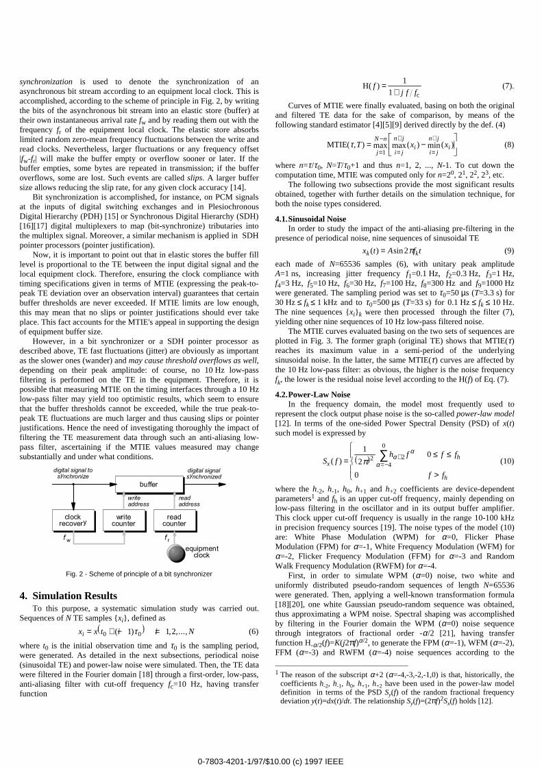
synchronization is used to denote the synchronization of anasynchronous bit stream according to an equipment local clock. This isaccomplished, according to the scheme of principle in Fig. 2, by writingthe bits of the asynchronous bit stream into an elastic store (buffer) attheir own instantaneous arrival rate fw and by reading them out with thefrequency fr of the equipment local clock. The elastic store absorbslimited random zero-mean frequency fluctuations between the write andread clocks. Nevertheless, larger fluctuations or any frequency offset|fw-fr| will make the buffer empty or overflow sooner or later. If thebuffer empties, some bytes are repeated in transmission; if the bufferoverflows, some are lost. Such events are called slips. A larger buffersize allows reducing the slip rate, for any given clock accuracy [14].

Hc

( )fj f f

=+

1

1(7).

Curves of MTIE were finally evaluated, basing on both the originaland filtered TE data for the sake of comparison, by means of thefollowing standard estimator [4][5][9] derived directly by the def. (4)

MTIE( )τ, max max( ) min( )T x xj

N n

i j

n j

ii j

n j

i= −�

!

"

$#

=

−

=

+

=

+

1(8)

where n=τ/τ0, N=T/τ0+1 and thus n=1, 2, ..., N-1. To cut down thecomputation time, MTIE was computed only for n=20, 21, 22, 23, etc.

The following two subsections provide the most significant resultsobtained, together with further details on the simulation technique, forboth the noise types considered.

Bit synchronization is accomplished, for instance, on PCM signalsat the inputs of digital switching exchanges and in PlesiochronousDigital Hierarchy (PDH) [15] or Synchronous Digital Hierarchy (SDH)[16][17] digital multiplexers to map (bit-synchronize) tributaries intothe multiplex signal. Moreover, a similar mechanism is applied in SDHpointer processors (pointer justification).

4.1.Sinusoidal NoiseIn order to study the impact of the anti-aliasing pre-filtering in the

presence of periodical noise, nine sequences of sinusoidal TE

x t A f tk k( ) sin= 2π (9)Now, it is important to point out that in elastic stores the buffer filllevel is proportional to the TE between the input digital signal and thelocal equipment clock. Therefore, ensuring the clock compliance withtiming specifications given in terms of MTIE (expressing the peak-to-peak TE deviation over an observation interval) guarantees that certainbuffer thresholds are never exceeded. If MTIE limits are low enough,this may mean that no slips or pointer justifications should ever takeplace. This fact accounts for the MTIE's appeal in supporting the designof equipment buffer size.

each made of N=65536 samples (6), with unitary peak amplitudeA=1 ns, increasing jitter frequency f1=0.1 Hz, f2=0.3 Hz, f3=1 Hz,f4=3 Hz, f5=10 Hz, f6=30 Hz, f7=100 Hz, f8=300 Hz and f9=1000 Hzwere generated. The sampling period was set to τ0=50 µs (T=3.3 s) for30 Hz ≤ fk ≤ 1 kHz and to τ0=500 µs (T=33 s) for 0.1 Hz ≤ fk ≤ 10 Hz.The nine sequences {xi} k were then processed through the filter (7),yielding other nine sequences of 10 Hz low-pass filtered noise.

The MTIE curves evaluated basing on the two sets of sequences areplotted in Fig. 3. The former graph (original TE) shows that MTIE(τ)reaches its maximum value in a semi-period of the underlyingsinusoidal noise. In the latter, the same MTIE(τ) curves are affected bythe 10 Hz low-pass filter: as obvious, the higher is the noise frequencyfk, the lower is the residual noise level according to the H(f) of Eq. (7).

However, in a bit synchronizer or a SDH pointer processor asdescribed above, TE fast fluctuations (jitter) are obviously as importantas the slower ones (wander) and may cause threshold overflows as well,depending on their peak amplitude: of course, no 10 Hz low-passfiltering is performed on the TE in the equipment. Therefore, it ispossible that measuring MTIE on the timing interfaces through a 10 Hzlow-pass filter may yield too optimistic results, which seem to ensurethat the buffer thresholds cannot be exceeded, while the true peak-to-peak TE fluctuations are much larger and thus causing slips or pointerjustifications. Hence the need of investigating thoroughly the impact offiltering the TE measurement data through such an anti-aliasing low-pass filter, ascertaining if the MTIE values measured may changesubstantially and under what conditions.

4.2.Power-Law NoiseIn the frequency domain, the model most frequently used to

represent the clock output phase noise is the so-called power-law model[12]. In terms of the one-sided Power Spectral Density (PSD) of x(t)such model is expressed by

S fh f f f

f f

xh

h

( ) =≤ ≤

>

%

&K

'K

+=−∑1

20

0

2 24

0

π αα

α0 5 (10)GLJLWDO�VLJQDO�WR�V\QFKURQL]H

GLJLWDO�VLJQDO�V\QFKURQL]HG

EXIIHU

FORFN�UHFRYHU\

ZULWHFRXQWHU

UHDGFRXQWHU

ZULWH�DGGUHVV

UHDG�DGGUHVV

HTXLSPHQW�FORFN

IZ I U

where the h-2, h-1, h0, h+1 and h+2 coefficients are device-dependentparameters1 and fh is an upper cut-off frequency, mainly depending onlow-pass filtering in the oscillator and in its output buffer amplifier.This clock upper cut-off frequency is usually in the range 10-100 kHzin precision frequency sources [19]. The noise types of the model (10)are: White Phase Modulation (WPM) for α=0, Flicker PhaseModulation (FPM) for α=-1, White Frequency Modulation (WFM) forα=-2, Flicker Frequency Modulation (FFM) for α=-3 and RandomWalk Frequency Modulation (RWFM) for α=-4.

Fig. 2 - Scheme of principle of a bit synchronizer First, in order to simulate WPM (α=0) noise, two white anduniformly distributed pseudo-random sequences of length N=65536were generated. Then, applying a well-known transformation formula[18][20], one white Gaussian pseudo-random sequence was obtained,thus approximating a WPM noise. Spectral shaping was accomplishedby filtering in the Fourier domain the WPM (α=0) noise sequencethrough integrators of fractional order -α/2 [21], having transferfunction H-α/2(f)=K(j2πf)α/2, to generate the FPM (α=-1), WFM (α=-2),FFM (α=-3) and RWFM (α=-4) noise sequences according to the

4. Simulation ResultsTo this purpose, a systematic simulation study was carried out.

Sequences of N TE samples {xi}, defined as

x x t i i Ni = + − =0 01 1 2( ) , ,...,τ1 6 (6)

where t0 is the initial observation time and τ0 is the sampling period,were generated. As detailed in the next subsections, periodical noise(sinusoidal TE) and power-law noise were simulated. Then, the TE datawere filtered in the Fourier domain [18] through a first-order, low-pass,anti-aliasing filter with cut-off frequency fc=10 Hz, having transferfunction

1 The reason of the subscript α+2 (α=-4,-3,-2,-1,0) is that, historically, the

coefficients h-2, h-1, h0, h+1, h+2 have been used in the power-law modeldefinition in terms of the PSD Sy(f) of the random fractional frequencydeviation y(t)=dx(t)/dt. The relationship Sy(f)=(2πf)2Sx(f) holds [12].

0-7803-4201-1/97/$10.00 (c) 1997 IEEE0-7803-4201-1/97/$10.00 (c) 1997 IEEE

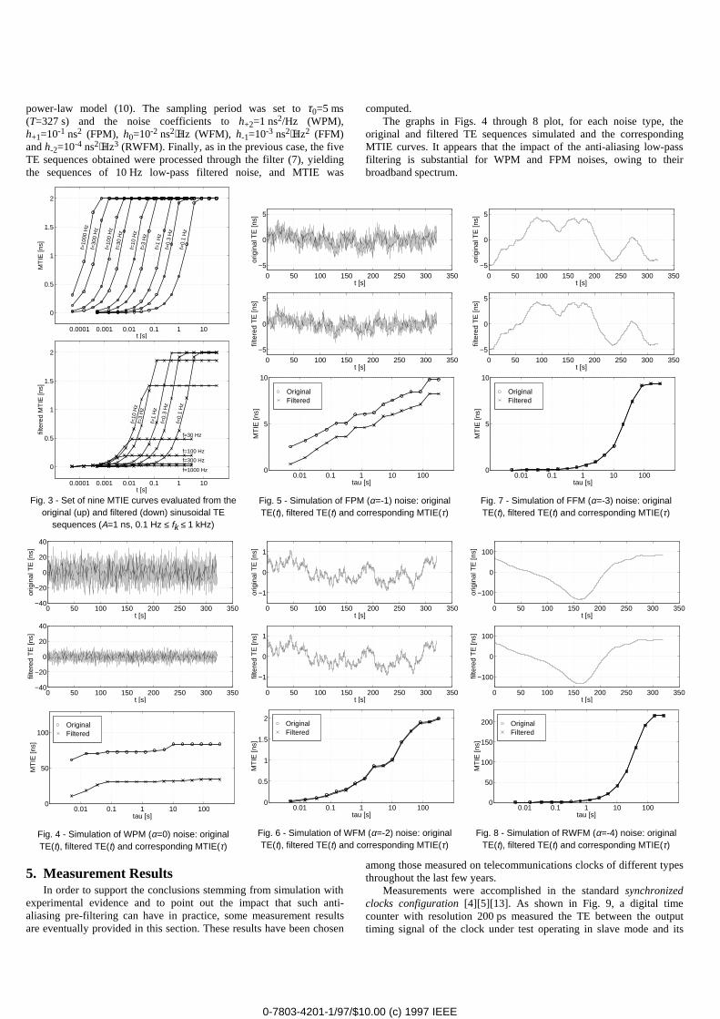
power-law model (10). The sampling period was set to τ0=5 ms(T=327 s) and the noise coefficients to h+2=1 ns2/Hz (WPM),h+1=10-1 ns2 (FPM), h0=10-2 ns2⋅Hz (WFM), h-1=10-3 ns2⋅Hz2 (FFM)and h-2=10-4 ns2⋅Hz3 (RWFM). Finally, as in the previous case, the fiveTE sequences obtained were processed through the filter (7), yieldingthe sequences of 10 Hz low-pass filtered noise, and MTIE was

computed.The graphs in Figs. 4 through 8 plot, for each noise type, the

original and filtered TE sequences simulated and the correspondingMTIE curves. It appears that the impact of the anti-aliasing low-passfiltering is substantial for WPM and FPM noises, owing to theirbroadband spectrum.

0.0001 0.001 0.01 0.1 1 10

0

0.5

1

1.5

2

MT

IE [n

s]

t [s]

f=0.

3 H

z

f=3

Hz

f=30

Hz

f=30

0 H

z

f=0.

1 H

z

f=1

Hz

f=10

Hz

f=10

0 H

z

f=10

00 H

z

0.0001 0.001 0.01 0.1 1 10

0

0.5

1

1.5

2

filte

red

MT

IE [n

s]

t [s]

f=1000 Hz

f=100 Hz

f=10

Hz

f=1

Hz

f=0.

1 H

z

f=300 Hz

f=30 Hz

f=3

Hz

f=0.

3 H

z

0 50 100 150 200 250 300 350

−5

0

5

t [s]

orig

inal

TE

[ns]

0 50 100 150 200 250 300 350

−5

0

5

t [s]

filte

red

TE

[ns]

0 50 100 150 200 250 300 350

−5

0

5

t [s]

orig

inal

TE

[ns]

0 50 100 150 200 250 300 350

−5

0

5

t [s]

filte

red

TE

[ns]

0.01 0.1 1 10 1000

5

10

tau [s]

MT

IE [n

s]

OriginalFiltered

0.01 0.1 1 10 1000

5

10

tau [s]M

TIE

[ns]

OriginalFiltered

Fig. 5 - Simulation of FPM (α=-1) noise: originalTE(t), filtered TE(t) and corresponding MTIE(τ)

Fig. 7 - Simulation of FFM (α=-3) noise: originalTE(t), filtered TE(t) and corresponding MTIE(τ)

Fig. 3 - Set of nine MTIE curves evaluated from theoriginal (up) and filtered (down) sinusoidal TE

sequences (A=1 ns, 0.1 Hz ≤ fk ≤ 1 kHz)

0 50 100 150 200 250 300 350−40

−20

0

20

40

t [s]

orig

inal

TE

[ns]

0 50 100 150 200 250 300 350−40

−20

0

20

40

t [s]

filte

red

TE

[ns]

0 50 100 150 200 250 300 350

−1

0

1

t [s]

orig

inal

TE

[ns]

0 50 100 150 200 250 300 350

−1

0

1

t [s]

filte

red

TE

[ns]

0 50 100 150 200 250 300 350

−100

0

100

t [s]

orig

inal

TE

[ns]

0 50 100 150 200 250 300 350

−100

0

100

t [s]

filte

red

TE

[ns]

0.01 0.1 1 10 1000

0.5

1

1.5

2

tau [s]

MT

IE [n

s]

OriginalFiltered

0.01 0.1 1 10 1000

50

100

150

200

tau [s]

MT

IE [n

s]

OriginalFiltered

0.01 0.1 1 10 1000

50

100

tau [s]

MT

IE [n

s]

OriginalFiltered

Fig. 6 - Simulation of WFM (α=-2) noise: originalTE(t), filtered TE(t) and corresponding MTIE(τ)

Fig. 8 - Simulation of RWFM (α=-4) noise: originalTE(t), filtered TE(t) and corresponding MTIE(τ)

Fig. 4 - Simulation of WPM (α=0) noise: originalTE(t), filtered TE(t) and corresponding MTIE(τ)

5. Measurement Resultsamong those measured on telecommunications clocks of different typesthroughout the last few years.

In order to support the conclusions stemming from simulation withexperimental evidence and to point out the impact that such anti-aliasing pre-filtering can have in practice, some measurement resultsare eventually provided in this section. These results have been chosen

Measurements were accomplished in the standard synchronizedclocks configuration [4][5][13]. As shown in Fig. 9, a digital timecounter with resolution 200 ps measured the TE between the outputtiming signal of the clock under test operating in slave mode and its

0-7803-4201-1/97/$10.00 (c) 1997 IEEE0-7803-4201-1/97/$10.00 (c) 1997 IEEE

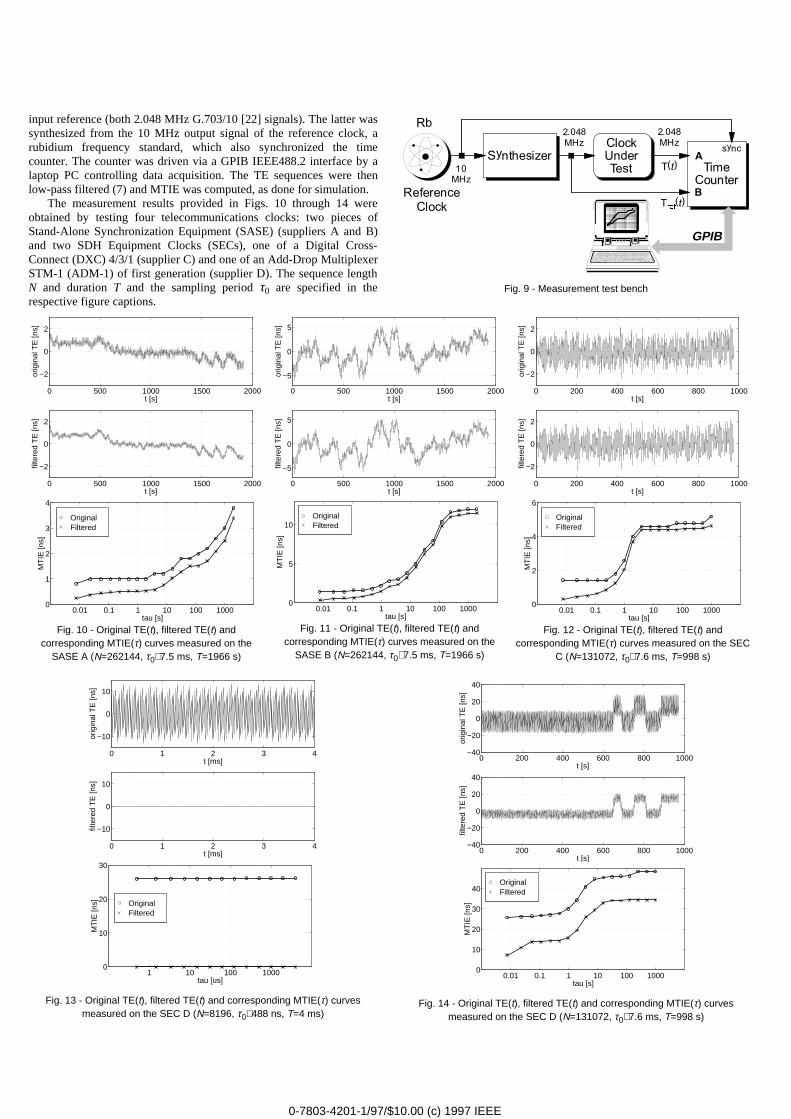
input reference (both 2.048 MHz G.703/10 [22] signals). The latter wassynthesized from the 10 MHz output signal of the reference clock, arubidium frequency standard, which also synchronized the timecounter. The counter was driven via a GPIB IEEE488.2 interface by alaptop PC controlling data acquisition. The TE sequences were thenlow-pass filtered (7) and MTIE was computed, as done for simulation.

&ORFN�8QGHU�7HVW

������0+]

������0+]

6\QWKHVL]HU7LPH�

&RXQWHU

V\QF$

%

7�W�

7����W�UHI

5HIHUHQFH�&ORFN

���0+]

5E

GPIB

The measurement results provided in Figs. 10 through 14 wereobtained by testing four telecommunications clocks: two pieces ofStand-Alone Synchronization Equipment (SASE) (suppliers A and B)and two SDH Equipment Clocks (SECs), one of a Digital Cross-Connect (DXC) 4/3/1 (supplier C) and one of an Add-Drop MultiplexerSTM-1 (ADM-1) of first generation (supplier D). The sequence lengthN and duration T and the sampling period τ0 are specified in therespective figure captions.

Fig. 9 - Measurement test bench

0 500 1000 1500 2000

−2

0

2

t [s]

orig

inal

TE

[ns]

0 500 1000 1500 2000

−2

0

2

t [s]

filte

red

TE

[ns]

0 500 1000 1500 2000

−5

0

5

t [s]

orig

inal

TE

[ns]

0 500 1000 1500 2000

−5

0

5

t [s]

filte

red

TE

[ns]

0 200 400 600 800 1000

−2

0

2

t [s]

orig

inal

TE

[ns]

0 200 400 600 800 1000

−2

0

2

t [s]

filte

red

TE

[ns]

0.01 0.1 1 10 100 10000

1

2

3

4

tau [s]

MT

IE [n

s]

OriginalFiltered

0.01 0.1 1 10 100 10000

5

10

tau [s]

MT

IE [n

s]

OriginalFiltered

0.01 0.1 1 10 100 10000

2

4

6

tau [s]

MT

IE [n

s]OriginalFiltered

Fig. 11 - Original TE(t), filtered TE(t) andcorresponding MTIE(τ) curves measured on the

SASE B (N=262144, τ0≅7.5 ms, T=1966 s)

Fig. 10 - Original TE(t), filtered TE(t) andcorresponding MTIE(τ) curves measured on the

SASE A (N=262144, τ0≅7.5 ms, T=1966 s)

Fig. 12 - Original TE(t), filtered TE(t) andcorresponding MTIE(τ) curves measured on the SEC

C (N=131072, τ0≅7.6 ms, T=998 s)

0 1 2 3 4

−10

0

10

t [ms]

orig

inal

TE

[ns]

0 1 2 3 4

−10

0

10

t [ms]

filte

red

TE

[ns]

0 200 400 600 800 1000−40

−20

0

20

40

t [s]

orig

inal

TE

[ns]

0 200 400 600 800 1000−40

−20

0

20

40

t [s]

filte

red

TE

[ns]

1 10 100 10000

10

20

30

tau [us]

MT

IE [n

s] OriginalFiltered

0.01 0.1 1 10 100 10000

10

20

30

40

tau [s]

MT

IE [n

s]

OriginalFiltered

Fig. 13 - Original TE(t), filtered TE(t) and corresponding MTIE(τ) curvesmeasured on the SEC D (N=8196, τ0≅488 ns, T=4 ms)

Fig. 14 - Original TE(t), filtered TE(t) and corresponding MTIE(τ) curvesmeasured on the SEC D (N=131072, τ0≅7.6 ms, T=998 s)

0-7803-4201-1/97/$10.00 (c) 1997 IEEE0-7803-4201-1/97/$10.00 (c) 1997 IEEE

The graphs shown exhibit a different behaviour according to theunderlying noise spectrum. The impact of the 10 Hz low-pass pre-filtering is always evident, but is substantial in particular in the case ofthe SEC D (Figs. 13 and 14), a Digital Phase-Locked Loop (DPLL)which deserves a closer look. This clock exhibits a wide and very fastperiodic noise, a saw-toothed TE waveform due to frequencyquantization error of peak-to-peak amplitude 25 ns and period 32 µs. Inthe measurement accomplished with sampling period τ0=488 ns (Fig.13), this noise gets completely cancelled by the 10 Hz low-pass filter,so that, while the filtered MTIE reports a reassuring 0 ns, the true MTIEis over 25 ns.

References[1] W. C. Lindsey, F. Ghazvinian, W. C. Hagmann and K. Dessouky,

"Network Synchronization", Proc. of the IEEE, vol. 73, no. 10,Oct. 1985, pp. 1445-1467.

[2] P. Kartaschoff, "Synchronization in Digital CommunicationsNetworks", Proc. of the IEEE, vol. 79, no. 7, July 1991, pp. 1019-1028.

[3] J. C. Bellamy, "Digital Network Synchronization", IEEE Comm.Mag., vol. 33, no. 4, Apr. 1995, pp. 70-83.

[4] ITU-T Rec. G.810 "Definitions and Terminology forSynchronisation Networks", Geneva, May 1996.

[5] ETSI Draft ETS 300 462 "Generic Requirements forSynchronisation Networks", Bonn, Sep. 1996.Considering the measurement accomplished with sampling period

τ0=7.6 ms (Fig. 14), on the other hand, it is interesting to notice that thefiltered MTIE curve does not start from the 0 ns level for τ=τ0, as itmight be expected on the basis of Fig. 13. The reason lies in thespectrum aliasing due to subsampling the saw-toothed noise: the aliasednoise is not fully filtered out due to its lower frequency. In spite of this,the filtered MTIE still reports a noise level three times smaller than theactual one.

[6] ITU-T Recs. G.810 "Considerations on Timing andSynchronization Issues", G.811 "Timing Requirements at theOutputs of Primary Reference Clocks Suitable for PlesiochronousOperation of International Digital Links", G.812 "TimingRequirements at the Outputs of Slave Clocks Suitable forPlesiochronous Operation of International Digital Links", BlueBook, 1988.

[7] ANSI T1.101-199X "Synchronization Interface Standard".[8] ITU-T Rec. G.813 "Timing Characteristics of SDH Equipment

Slave Clocks (SEC)", Geneva, May 1996.6. Conclusions [9] S. Bregni, "Measurement of Maximum Time Interval Error for

Telecommunications Clock Stability Characterization", IEEETrans. Instrum. Meas., vol. IM-45, no. 5, Oct. 1996.The impact on MTIE of filtering the TE measurement data through

a first-order, low-pass, anti-aliasing filter with cut-off frequency fc=10Hz was thoroughly studied through a simulation approach, bygenerating TE sequences affected by periodical noise (sinusoidal TE)and by power-law noise. The simulation results showed in particularthat the impact of anti-aliasing pre-filtering may be substantial for sometypes of noise (namely, WPM and FPM), owing to their broadbandspectrum.

[10] S. Bregni and P. Tavella, "Estimation of the Percentile MaximumTime Interval Error of Gaussian White Phase Noise", Proc. ofIEEE ICC '97, Montréal, Québec, Canada, June 1997.

[11] J. A. Barnes, A. R. Chi, L. S. Cutler, D. J. Healey, D. B. Leeson, T.E. McGunigal, J. A. Mullen Jr., W. L. Smith, R. L. Sydnor, R. F.C. Vessot and G. M. R. Winkler, "Characterization of FrequencyStability", IEEE Trans. Instrum. Meas., vol. IM-20, no. 2, May1971.

Moreover, some results of measurements on varioustelecommunications clocks have been provided. The results shownpoint out that the impact that such anti-aliasing pre-filtering can have inpractice on clocks may be substantial and even misleading:measurements accomplished through such filter may produce toooptimistic results, hiding the true amplitude of TE fluctuations at timinginterfaces, and therefore may yield errors in buffer size design or inassessing the pointer justification rate in SDH transmission chains.

[12] J. Rutman and F. L. Walls, "Characterization of FrequencyStability in Precision Frequency Sources", Proc. of the IEEE, vol.79, no. 7, pp. 952-960, July 1991.

[13] M. Carbonelli, D. De Seta and D. Perucchini, "Characterization ofTiming Signals and Clocks", European Trans. on Telecommun.,vol. 7, no. 1, Jan.-Feb. 1996.

[14] H. L. Hartmann, E. Steiner, "Synchronization Techniques forDigital Networks", IEEE Journal on Sel. Areas in Commun., vol.SAC-4, no. 4, July 1986, pp. 506-513.

[15] ITU-T Rec. G.702 "Digital Hierarchy Bit Rates", Blue Book,Geneva 1988.

Acknowledgements [16] ITU-T Revised Rec. G.707 "Network Node Interface for theSynchronous Digital Hierarchy (SDH)", Geneva, March 1996.The measurement data were acquired out while Stefano Bregni was

with the R&D Div. of SIRTI (Italy), in the framework of the activitiespromoted by the National Study Group on Synchronization (establishedby Telecom Italia and joined by SIRTI, Fondazione Ugo Bordoni andCSELT). A special note of thanks is due to Luca Valtriani (formerlywith SIRTI, now Director of Technical Planning Dept. in TelecomArgentina). Moreover, the Authors wish to thank Elio Bava(Politecnico di Milano) for his continuing support.

[17] M. Sexton and A. Reid, "Broadband Networking: ATM, SDH andSONET". Norwood, MA: Artech House, 1997.

[18] S. Bregni, L. Valtriani and F. Veghini, "Simulation of Clock Noiseand AU-4 Pointer Action in SDH Equipment", in Proc. of IEEEGLOBECOM '95, Singapore, Nov. 1995.

[19] Fred L. Walls and A. De Marchi, "RF Spectrum of a Signal afterFrequency Multiplication: Measurement and Comparison with aSimple Calculation", IEEE Trans. Instrum. Meas., vol. IM-24, no.3, Sept. 1975.

[20] D. E. Knuth, "The Art of Computer Programming", vol. 2, p. 118.London: Addison-Wesley, 1981.

[21] J. A. Barnes, D. W. Allan, "A Statistical Model of Flicker Noise",Proc. of the IEEE, vol. 54, no. 2, pp. 176-178, Feb. 1966.

[22] ITU-T Rec. G.703 "Physical/Electrical Characteristics ofHierarchical Digital Interfaces", Blue Book, Geneva 1988.

0-7803-4201-1/97/$10.00 (c) 1997 IEEE