TAMPERE UNIVERSITY OF TECHNOLOGY Institute of Communications Engineering FRANCESC BORRS TOR Impact of Antenna Beamwidth, Propagation Slope and Coverage Overlapping on Capacity in WCDMA Networks Diplomity Master of Science Thesis Subject approved by the department council on 4.06.2003 Supervisor: Prof. Jukka Lempiinen

Welcome message from author
This document is posted to help you gain knowledge. Please leave a comment to let me know what you think about it! Share it to your friends and learn new things together.
Transcript

TAMPERE UNIVERSITY OF TECHNOLOGY Institute of Communications Engineering
FRANCESC BORRÀS TORÀ
Impact of Antenna Beamwidth,
Propagation Slope and Coverage
Overlapping on Capacity in WCDMA
Networks Diplomityö Master of Science Thesis Subject approved by the department council on 4.06.2003 Supervisor: Prof. Jukka Lempiäinen

Preface The work for this Master´s thesis was carried out in the radio communications group, in
the Institute of Communications Engineering, at Tampere University of Technology
(TUT), in the project �Planning and Topology of 3G Networks�.
I would like to thank Professor Jukka Lempiäinen for his help and my friend Jarno
Niemelä for his patience, personal abnegation and valuable support during my work. In
addition, I would like to thank all TUT personal: Sami (systems administrator), Tarja
(department secretary) and so many others for their efficiency and exquisite manner
during this wonderful year.
Furthermore, I would like to thank my roommate at TUT, Tuomo Kuusisto, for his
pleasant company, co-operation and fruitful working environment during all these
months.
I would also like to thank my home university in Barcelona, Universitat Politècnica de
Catalunya (UPC), for all these years of learning in an extraordinary environment.
Moreover, I would like to thank my sister Neus Borràs for her dedication and valuable
contribution for the fulfilment of this work and my girlfriend Mercè Gabaldà for her
patience during my stay in Finland.
Finally, I would specially like to thank my parents for their touching love, support and
understanding during my studies, since without this nothing would have been possible.
Tampere (Finland), 16.06.2003
Francesc Borràs Torà [email protected]
Colon 13
43748 Ginestar (Tarragona)
SPAIN
Telephone: + 34 977 409 041
ABSTRACT 3
Abstract
TAMPERE UNIVERSITY OF TECHNOLOGY Degree program in Information Technology Telecommunication Engineering Borràs Torà, Francesc: Impact of Antenna Beamwidth, Propagation Slope and Coverage Overlapping on Capacity in WCDMA Networks Master of Science thesis, 104 p. Examiner: Prof. Jukka Lempiäinen Institute of Communications Engineering August 2003 Keywords: UMTS, WCDMA, radio network planning, antenna beamwidth, antenna height, cell range, sectorisation Mobile communications sector has experienced a great growth during 1990�s. Nowadays, tendency is to provide global coverage and high capacity for high speed data services in a more flexible way. Universal Mobile Telecommunications System (UMTS) has been standardized to provide high capacity and global coverage. The air interface selected for UMTS is Wideband Code Division Multiple Access (WCDMA). This solution offers to operators a big number of significant advantages over alternative technologies, including increased network capacity, longer battery life for terminals and enhanced privacy for users. However, such benefits come at the cost of additional network complexity. This is why a background in GSM deployment is no guarantee of success in UMTS. Last estimates are that operator spending on the radio network planning of UMTS system will account for more than 60% of total capital expenditure. For this reason a robust network implementation (correct choices for key parameters like antenna beamwidth, antenna height, number of sectors/site, etc.) is critical if operators want to optimize capacity levels and enable multimedia services, which are a key element of the UMTS value proposition. In this work, impact on coverage and capacity of the system for different network configurations is investigated by using Nokia Networks static radio network planning tool NetAct WCDMA Planner 4.0, which uses Monte-Carlo simulations. After completed all these simulations, results are analysed and main conclusions are explained in order to make easier future works in the same area. To conclude, point out something significant: air interface technology (WCDMA), basic algorithms and radio network planning techniques are radically different respect to GSM, therefore, operators must demonstrate technical leadership and deployment experience in all these aspects. Only then can they expect to achieve the required levels of radio performance for tomorrow´s 3G services.

TIIVISTELMÄ 4
Tiivistelmä
TAMPEREEN TEKNILLINEN YLIOPISTO Tietotekniikan koulutusohjelma Tietoliikennetekniikan laitos Borràs Torà, Francesc: Antennin keilanleveyden, etenemiskertoimen ja peiton limittäisyyden vaikutus WCDMA verkon kapasiteettiin Diplomityö, 104 s. Tarkastaja: Prof. Jukka Lempiäinen Elokuu 2003 Avainsanat: UMTS, WCDMA, radioverkkosuunnittelu, antennin keilanleveys, antennin korkeus, solun säde, sektorointi Matkaviestinjärjestelmät ovat kokeneet suuren kasvun 1990-luvun aikana. Tänä päivänä suuntaus on tuoda käyttäjien ulottuville maailmanlaajuinen peitto ja korkeat datanopeudet joustavalla tavalla. Universal Mobile Telecommunication Systems (UMTS) on standartoitu täyttämään nämä odotukset korkeasta kapasiteetista ja maailmankattavasta peitosta. UMTS:n ilmarajapinnan pääsytekniikaksi valittiin laajakaistainen koodijakotekniikka (Wideband Code Division Multipe Access, WCDMA). Tämä tekniikka tarjoaa operaattoreille lukemattomia etuja vaihtoehtoisien tekniikkojen lisäksi. Näitä ovat mm. parantunut verkon kapasiteetti, matkapuhelimen akun pidentynyt käyttöaika ja käyttäjien yksityisyyden parantuminen. Parannukset ovat kuitenkin aiheuttaneet verkon kompleksisuuden kasvun. Tämän vuoksi GSM-verkon kaltaisella radioverkkosuunnittelulla ei taata menestystä UMTS-verkkosuunnittelun saralla. Viimeisimmän arvion mukaan yli 60% operaattorien kustannuksista aiheutuu UMTS-radioverkkon implementoinnista. Tämän vuoksi joustava radioverkon implmentointi (tärkeiden verkkoparametrien määrittäminen kuten antennin keilanleveyden, antennin korkeuden, sektoreiden lukumäärän jne.) on kriittistä, mikäli operaattorit haluavat optimoida verkon kapasiteetin ja tarjota multimedia palveluita, jotka ovat UMTS verkon uusia, keskeisiä ominaisuuksia. Tässä diplomityössä on tutkittu eri verkkokonfiguraatioiden vaikutusta radioverkon peitoon ja kapasitteettiin käyttämällä Nokia Networks:in Monte-Carlo �simulaatioita hyödyntäävää radioverkkosuunnitteluohjelmaa NetAct WCDMA Planner 4.0. Tulosten analysointi ja johtopäätöset on tehty helpottamaan tulevaisuuden verkkosuunnittelua. Tärkeäksi lopputulokseksi on saatu, että ilmarajapinnan pääsytekniikka (WCDMA), perus algoritmit ja radioverkkon suunnittelutekniikka ovat erilaisia verrattuna GSM:ään, ja sen vuoksi operaattoreiden on hyödynnettävä kaikkea teknista osaamista ja kokemusta näiltä saroilta. Vasta tämän jälkeen he voivat saavuttaa vaaditut suorituskykyvaatimukset huomisen 3G-palveluille.

EXTRACTE 5
Extracte
UNIVERSITAT TECNOLÒGICA DE TAMPERE Programa de graduació en Tecnologies de la Informació Enginyeria de Telecomunicació Borràs Torà, Francesc: Impacte de l´Ample de Feix de les Antenes, de les Pèrdues de Propagació i del Solapament de la Cobertura sobre la Capacitat de Xarxes WCDMA Projecte Final de Carrera, 104 p. Examinador: Prof. Jukka Lempiäinen Institut d´Enginyeria de les Comunicacions Agost 2003 Paraules clau: UMTS, WCDMA, planificació de xarxes ràdio, ample de feix, alçada d´antena, tamany de cel.la, sectorització El sector de les comunicacions mòbils ha experimentat un gran creixement durant els anys 90. Actualment, la tendència és proporcionar cobertura global i gran capacitat d´una forma més flexible per serveis de dades d´alta velocitat. El Sistema Universal de Telecomunicacions Mòbils (UMTS) ha estat estandaritzat per proporcionar alta capacitat i cobertura global. La interfície aèria sel.leccionada per UMTS és Accés Múltiple per Divisó de Codi en Banda Ampla (WCDMA). Aquesta solució ofereix als operadors un gran nombre de significatius avantatges sobre tecnologies alternatives, incloent major capacitat de la xarxa, vida més llarga per les bateries dels terminals i augment d´intimitat pels usuaris. No obstant, aquests beneficis arriben gràcies al cost de complexitat addicional de la xarxa. Aquest és el motiu pel qual l´experiència en GSM no és garantia d´èxit en UMTS. Les últimes estimacions indiquen que la despesa d´un operador en la planificació de xarxes ràdio UMTS superarà més del 60% del capital total invertit. Per aquesta raó una implementació robusta de la xarxa (el.leccions correctes per paràmetres clau com ample de feix de les antenes, alçada de les mateixes, nombre de sectors/cel.la, etc.) és crítica si els operadors volen optimitzar els nivells de capacitat i activar serveis multimèdia, els quals són un element clau del valor de la proposició UMTS. En aquest treball s´estudia l´impacte sobre la cobertura i la capacitat del sistema per diferents configuracions de la xarxa, utilitzant l´eina estàtica de planificació de xarxes ràdio de Nokia Networks, el NetAct WCDMA Planner 4.0, el qual utilitza simulacions Monte-Carlo. Després de completar aquestes simulacions, els resultats són analitzats, explicant les principals conclusions per tal de fer més fàcils futurs treballs en la mateixa àrea. Per acabar, assenyalar quelcom significatiu: la interfície aèria (WCDMA), els algoritmes bàsics i les tècniques de planificació de xarxes ràdio són radicalment diferents respecte a GSM, per tant, els operadors han de demostrar liderat tècnic i experiència en el desplegament en tots aquests aspectes. Només llavors poden esperar aconseguir els nivells de prestació exigits pels serveis de tercera generació del futur.

CONTENTS 6
CONTENTS
PREFACE........................................................................................................................ 2
ABSTRACT..................................................................................................................... 3
TIIVISTELMÄ ............................................................................................................... 4
EXTRACTE .................................................................................................................... 5
1.- INTRODUCTION ..................................................................................................... 8
2.- UMTS.......................................................................................................................... 10
2.1.- STANDARDIZATION ....................................................................................... 11
2.2.- QoS CLASSES .................................................................................................... 11
2.3.- NETWORK ARCHITECTURE.......................................................................... 13
2.3.1.- UMTS RADIO ACCESS NETWORK........................................................ 14
2.3.2.- CORE NETWORK...................................................................................... 14
2.4.- CHANNEL STRUCTURE.................................................................................. 15
3.- WCDMA RADIO ACCESS...................................................................................... 21
3.1.- MULTIPLE ACCESS ......................................................................................... 22
3.2.- CDMA ................................................................................................................. 23
3.3.- DS-CDMA........................................................................................................... 25
3.4.- WCDMA.............................................................................................................. 33
3.4.1.- RADIO PROPAGATION CHARACTERISTICS IN WCDMA ................ 37
4.- PLANNING OF WCDMA RADIO NETWORKS................................................. 43
4.1.- DIMENSIONING................................................................................................ 44
4.2.- DETAILED PLANNING .................................................................................... 46
4.2.1.- CONFIGURATION PLANNING................................................................ 46
4.2.2.- COVERAGE PREDICTIONS ..................................................................... 52
4.2.3.- TOPOLOGY PLANNING ........................................................................... 57
4.3.- OPTIMIZATION................................................................................................. 61
4.4.- CELL TYPES ...................................................................................................... 61
5.- SIMULATIONS......................................................................................................... 65
5.1.- SIMULATION SETUP ....................................................................................... 66

CONTENTS 7
5.2.- RESULTS............................................................................................................ 69
5.2.1.- SCENARIO 1: 3-SECTOR CASE .............................................................. 70
5.2.2.- SCENARIO 2: 6-SECTOR CASE .............................................................. 76
5.2.3.- OPTIMUM CONFIGURATIONS .............................................................. 82
6.- CONCLUSIONS........................................................................................................ 86
7.- REFERENCES .......................................................................................................... 89
APPENDIX...................................................................................................................... 94
List of Acronyms ......................................................................................................... 94
List of Tables ............................................................................................................... 98
List of Figures .............................................................................................................. 99
Simulation Parameters ............................................................................................... 102
1.- INTRODUCTION 8
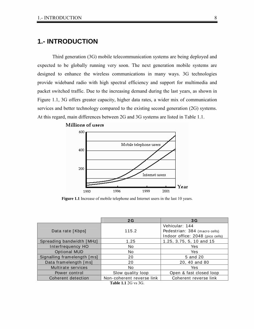
1.- INTRODUCTION Third generation (3G) mobile telecommunication systems are being deployed and
expected to be globally running very soon. The next generation mobile systems are
designed to enhance the wireless communications in many ways. 3G technologies
provide wideband radio with high spectral efficiency and support for multimedia and
packet switched traffic. Due to the increasing demand during the last years, as shown in
Figure 1.1, 3G offers greater capacity, higher data rates, a wider mix of communication
services and better technology compared to the existing second generation (2G) systems.
At this regard, main differences between 2G and 3G systems are listed in Table 1.1.
Figure 1.1 Increase of mobile telephone and Internet users in the last 10 years.
2G 3G
Data rate [Kbps]
115.2 Vehicular: 144 Pedestrian: 384 (macro cells) Indoor office: 2048 (pico cells)
Spreading bandwidth [MHz] 1.25 1.25, 3.75, 5, 10 and 15 Interfrequency HO No Yes
Optional MUD No Yes Signalling framelength [ms] 20 5 and 20
Data framelength [ms] 20 20, 40 and 80 Multirate services No Yes
Power control Slow quality loop Open & fast closed loop Coherent detection Non-coherent reverse link Coherent reverse link
Table 1.1 2G vs 3G.

1.- INTRODUCTION 9
The new wideband characteristics and the flexibility to introduce new services
will be exploited in a variety of mobile devices and innovative seamless applications.
Examples of the proposed services include multimedia applications such as mobile video
conferencing and web browsing. Nevertheless, there will probably not be any single
application that is going to dominate the next generation market, and it is expected that
3G will breed success through its flexibility and a wide range of personal services.
Nonetheless, 3G systems will have a very high potential because they will be able to
support various simultaneous connections, for example speech, Internet connection and
videoconference, with high quality, especially in voice services.
Wideband code division multiple access (WCDMA) has emerged as a main
stream air interface solution for the next generation networks. It has been also selected as
a radio transmission technology (RTT) for UMTS (Universal Mobile
Telecommunications System), which is the european third generation mobile
communications system developed by ETSI (European Telecommunications Standards
Institute).
The most essential elements of the third generation mobile systems have been
already standardized, and basic operational requirements and system architecture are
already well understood. However, there is plenty of room for innovations and
enhancements in many areas within 3G.
This thesis is organized using the top-down approach. First, a general introduction
to UMTS is presented in chapter 2. Then, chapter 3 gives a presentation of the WCDMA
principles, including radio propagation characteristics in WCDMA networks. Radio
network planning for 3G systems is studied in chapter 4. Described planning is enough to
illustrate the basic used mechanisms for an operator in its network design. This chapter
introduces the main purpose of this thesis: study the impact of antenna beamwidth,
propagation slope and coverage overlapping on capacity in WCDMA cellular networks.
This analysis is covered in detail in the next chapter, number 5, by using a static radio
network planning tool provided by Nokia Networks: NetAct WCDMA Planner 4.0, which
uses Monte-Carlo simulations. Finally, conclusions are presented in chapter 6.

2.- UMTS 10
2.- UMTS
UMTS (Universal Mobile Telecommunications System) is one of the major new
third generation mobile communications systems being developed within the framework,
which has been defined by ITU (International Telecommunications Union) and known as
IMT-2000 (International Mobile Telephony). UMTS facilitates convergence between
telecommunications, IT, media and content industries. It has potential to provide end
users with data rates up to 2 Mbps, and it lends itself to give individuals the freedom to
choose among a wide range of services currently in existence or soon to exist. Some
examples of the new services are video telephony and quick access to information and
fast data downloads, for instance, on Internet directly for people on the move.
In this chapter, the standardization process for the 3rd generation mobile
telecommunications system and the different varieties of quality of service on it are
explained. After this, used network architecture and channel structure in this system are
shown in order to understand clearly how it works.

2.- UMTS 11
2.1.- STANDARDIZATION
International Telecommunications Union is coordinating 3G standardization.
Within ITU, the third generation systems are called International Mobile Telephony
2000. Regional standardization organizations, such as ETSI in Europe, have specified
their proposals to fulfil the IMT-2000 requirements. The third generation system is called
UMTS within ETSI.
In the standardization forums, wideband CDMA has emerged as the most widely
adopted third generation air interface [1]. In addition, ETSI selected WCDMA as the
basic access scheme in January 1998. WCDMA specification is produced in 3GPP (Third
Generation Partnership Project) [2], which is the joint standardization project of the
standardization bodies from Europe, Japan, Korea, the USA and China.
Nowadays (June´03), UMTS licenses have been awarded in more than fifteen
countries. Experimental systems are made with field trials and commercial services are
being launched in Japan and other places. Standards and industrial interest groups
mentioned above can be found in [3-6]. 2.2.- QoS CLASSES
UMTS has been designed to support a variety of quality of service (QoS)
requirements that are set by end users and end-user applications. The third generation
services will vary from simple voice telephony to more complex data applications
including voice over IP (VoIP), video conferencing over IP (VCoIP), web browsing, e-
mail and file transfer. 3GPP has identified four different main traffic classes for UMTS
according to the nature of traffic: conversational class, streaming class, interactive class
and background class [7].
The best-known use of conversational class is telephony speech. With Internet
and multimedia, a number of new applications, for example, VoIP and video
conferencing tools will require this scheme. Real time conversation is always performed
between peers of human end users. This is the only traffic type where the required
characteristics are strictly imposed by human perception. Real time conversation is

2.- UMTS 12
characterized by the fact that the transfer time and time variation between information
entities must be low and preserved.
Streaming class is applied when the transferred data is processed as a steady and
continuous stream. Accordingly, the streaming class is characterized by the preserved
time variation between information entities of the stream, but it does not have any
requirements on low transfer delay. Thus, the acceptable delay variation over
transmission media (jitter) is much higher than in the conversational class. An example of
this scheme is the user looking at real-time video or listening to real-time audio.
When the end user, either a machine or human, is on-line requesting data from
remote equipment (i.e., a server), interactive class scheme applies. Examples of
interactive human interaction with remote equipment are web browsing, database
retrieval and server access. Examples of machine interaction with remote equipment are
polling for measurement records and automatic database enquiries. Interactive class is
characterized by request response pattern (round trip delay and response time) and
preserved payload content (low Bit Error Rate). Applications such as e-mail and SMS,
download of databases and reception of measurement records generate distinctive
background class traffic. Background traffic scheme is characterized by the fact that the
destination is not expecting the data within a certain time, but that the data integrity must
be preserved during the delivery. The UMTS QoS classes are summarized in Table 2.1.
TRAFFIC CLASS Conversational Class
Streaming Class
Interactive Class
Background Class
FUNDAMENTAL CHARACTERISTICS
• Preserve time relation (variation) between information entities of the stream
• Conversational pattern (stringent & low delay)
• Preserve time relation (variation) between information entities of the stream
• Request response pattern
• Preserve payload content
• Destination is not expecting the data within a certain time
• Preserve
payload content
EXAMPLE OF APPLICATION
- Voice - Video
telephony - Video games
- Streaming multimedia
- Web browsing
- Network games
- Background download of e-mails
Table 2.1 QoS classes in UMTS.

2.- UMTS 13
The requirements of the QoS classes are met by negotiating appropriate QoS
attribute values for each established or modified UMTS bearer. Traffic parameter set
consists of eight different attributes: maximum bit rate (Kbps), guaranteed bit rate
(Kbps), delivery order (yes/no), SDU (Service data unit) size information (bits),
reliability, transfer delay (seconds), traffic handling priority and allocation/retention
policy [7].
2.3.- NETWORK ARCHITECTURE
UMTS network architecture will be an evolution of GSM and GPRS network,
thus resembling very much of their architecture. It consists of two parts: UMTS terrestrial
radio access network (UTRAN) and core network (CN).
UTRAN provides the air interface for UMTS terminals and core network is
responsible for switching and routing of calls and data connections to external networks.
The UMTS system architecture with the interfaces is depicted, by using a tree diagram, in
Figure 2.1 [8]. The interfaces are defined open to allow the equipment at the endpoints to
be from two different manufacturers. A complete description of the network architecture
and the interfaces between the logical network elements can be found in 3GPP technical
specifications (TS) [3].
Figure 2.1 UMTS network architecture.

2.- UMTS 14
2.3.1.- UMTS Radio Access Network
UTRAN consists of one or more radio network subsystems (RNS). Each radio
network subsystem consists of a radio network controller (RNC), several nodes B
(UMTS base stations) and user equipment (UE).
The radio network controller is responsible for the control of radio resources of
UTRAN. It plays a very important role in power control (PC), handover control (HC),
admission control (AC), load control (LC) and packet scheduling (PS) algorithms, which
are at least partially located at RNC. RNC interfaces the core network via Iu interface and
uses Iub to control one node B. The Iur interface between RNCs allows soft handover
between RNCs.
Node B is equivalent to the GSM base station (BS/BTS), and it is the physical
unit for radio transmission and reception with cells. Node B performs the air interface
processing, which includes channel coding, interleaving, rate adaptation and spreading.
The connection with the user equipment is made via Uu interface, which is actually the
WCDMA radio interface. Node B takes part in softer handover process and it is also
responsible for inner closed-loop power control. User equipment is based on the same
principles as the GSM mobile station (MS), and it consists of two parts: mobile
equipment (ME) and the UMTS subscriber identity module (USIM). Mobile equipment is
the device that provides for radio transmission, and the USIM is the smart card holding
the user identity and personal information.
2.3.2.- Core Network
UMTS is based on an evolved core GSM network integrating circuit and packet
switched traffic. The entities of CN, shown in Figure 2.2, are home location register
(HLR), mobile services switching center/visitor location register (MSC/VLR), gateway
MSC (GMSC), serving GPRS support node (SGSN) and gateway GPRS support node
(GGSN).
The home location register is a database in charge of the management of mobile
subscribers. It holds the subscriber and location information enabling the charging and
routing of calls towards the MSC or SGSN, where the mobile station is registered at that
time.

2.- UMTS 15
The mobile switching center constitutes the interface between the radio system
and the fixed networks. The MSC performs all necessary functions in order to handle the
circuit switched services to and from the mobile stations. A mobile station roaming in an
MSC area is controlled by the visitor location register in charge of this area.
Gateway MSC is the switch at the point where UMTS public land mobile network
(PLMN) is connected to external circuit switched networks. All incoming and outgoing
circuit switched connections go through GMSC.
Serving GPRS support node has similar functionality to that of MSC/VLR, but it
is used for packet switched services. Gateway GPRS support node has the same
functionality for the packet domain as the GMSC has for the circuit domain.
All these elements and their interconnections are shown in Figure 2.2.
Figure 2.2 Block diagram of the UTRAN and CN.
2.4.- CHANNEL STRUCTURE
There are two dedicated channels and one common channel on the uplink. User
data is transmitted on the dedicated physical data channel (DPDCH). Control information
is transmitted on the dedicated physical data channel (DPDCH) too. The random access
channel is a common access channel.
Each DPDCH frame on a single code carries 160 x 2k bits (16 x 2k Kbps), where k
changes between 0, 1, ... and 6, corresponding to a spreading factor of 256/2k with the

2.- UMTS 16
3.84 Mcps of chip rate. Multiple parallel variable rate services can be time multiplexed
within each DPDCH frame. The overall DPDCH bit rate is variable on a frame-by-frame
basis. In most cases, only one DPDCH is allocated per connection, and services are
jointly interleaved sharing the same DPDCH. However, multiple DPDCHs can also be
allocated (e.g. to avoid a too low spreading factor at high data rates).
The dedicated physical control channel (DPCCH) is needed to transmit pilot
symbols for coherent reception, power control signaling bits and rate information for rate
detection. Two basic solutions for multiplexing physical control and data channels are
time multiplexing and code multiplexing. A combined IQ and code multiplexing solution
(dual-channel QPSK) is used in WCDMA uplink to avoid electromagnetic compatibility
(EMC) problems with discontinuous transmission (DTX). The major drawbacks of the
time multiplexed control channel are the EMC problems that arise when DTX is used for
user data. One example of a DTX service is speech. During silent periods no information
bits need to be transmitted, which results in pulsed transmission as control data must be
transmitted in any case.
The rate of transmission of pilot and power control symbols causes severe EMC
problems to both external equipment and terminal interiors. This EMC problem is more
difficult in the uplink direction since mobile stations can be close to other electrical
equipments. The IQ code multiplexed control channel is shown in Figure 2.3.
Figure 2.3 Parallel transmission of DPDCH and DPDCCH channels when data is present/absent.
Since pilot and power control are on a separate channel, no pulse like
transmission takes place. Interference to other users and cellular capacity remains the
same as in the time multiplexed solution.

2.- UMTS 17
The random access burst consists of two parts, a preamble part of length 16 x 256
chips (1 ms) and a data part of variable length. The WCDMA random access scheme is
based on a slotted ALOHA technique with the random access burst structure as shown in
Figure 2.4.
Figure 2.4 Structure of WCDMA random access burst.
Before the transmission of a random access request, the mobile terminal should
carry out the following tasks:
• Achieve chip, slot and frame synchronization to the target base station from the
synchronization channel (SCH) and obtain information about the downlink scrambling
code also from the SCH.
• Retrieve information from BCCH about the random access code(s) used in the target
cell/sector.
• Estimate the downlink path loss, which is used together with a signal strength target to
calculate the required transmit power of the random access request.
It is possible to transmit a short packet together with a random access burst
without setting up a scheduled packet channel. No separate access channel is used for
packet traffic related random access, but all traffic shares the same random access
channel. More than one random access channel can be used if the random access capacity
requires such an arrangement [9].
2.- UMTS 18
In the downlink, there are three common physical channels. The primary and
secondary common control physical channels (CCPCH) carry the downlink common
control logical channels (BCCH, PCH and FACH), finally, the SCH provides timing
information and is used for handover measurements by the mobile station.
The dedicated channels (DPDCH and DPCCH) are time multiplexed. The EMC
problem caused by discontinuous transmission is not considered difficult in downlink
since there are signals to several users transmitted in parallel at the same time and base
stations are not so close to other electrical equipment.
In the downlink, time multiplexed pilot symbols are used for coherent detection.
Since the pilot symbols are connection dedicated, they can be used for channel estimation
and to support downlink fast power control. In addition, a common pilot time multiplexed
in the BCCH channel can be used for coherent detection.
The primary CCPCH carries the BCCH channel and a time multiplexed common
pilot channel. The primary CCPCH is allocated at the same channelization code in all
cells. A mobile terminal can thus always find the BCCH, once the base station's unique
scrambling code has been detected during the initial cell search.
The secondary physical channel for common control carries the PCH and FACH
in time multiplex within the super frame structure. The channelization code of the
secondary CCPCH is transmitted on the primary CCPCH. The SCH consists of two
subchannels, the primary and secondary SCHs. The SCH minimizes the acquisition time
of the long code. The unmodulated primary SCH is used to acquire the timing for the
secondary SCH. The modulated secondary SCH code carries information about the long
code group to which the long code of the BS belongs. In this way, the search of long
codes can be limited to a subset of all the codes.
The primary SCH consists of an unmodulated code of length 256 chips, which is
transmitted once in every slot. The primary synchronization code is the same for every
base station in the system and is transmitted time aligned with the slot boundary. The
secondary SCH consists of one modulated code of length 256 chips, which is transmitted
in parallel with the primary SCH.
Multiple services of the same connection are multiplexed on one DPDCH.
Multiplexing may take place either before or after the inner or outer coding. After service

2.- UMTS 19
multiplexing and channel coding, the multiservice data stream is mapped to one DPDCH.
If the total rate exceeds the upper limit for single code transmission, several DPDCHs can
be allocated [9].
Typical power allocations for the downlink common channels are shown in Table
2.2 .
Activity
[%]
Percentage of
the maximum
base station
power
[%]
Power allocation
with 20 W.
maximum power
[W]
Common pilot channel
(CPICH)
100
10
2.0
Primary synchronization
channel (SCH)
10
6
1.2
Secondary synchronization
channel (SCH)
10
4
0.8
Primary common control
physical channel (CCPCH)
90
5
1.0
Total common channels - ~ 15 ~ 3
Table 2.2 Typical powers for the downlink common channels.
WCDMA has two different types of packet data transmission possibilities. Short
data packets can be appended directly to a random access burst. This method, called
common channel packet transmission, is used for short infrequent packets, where the link
maintenance needed for a dedicated channel would lead to an unacceptable overhead.
When using the uplink common channel, a packet is appended directly to a
random access burst. Also, the delay associated with a transfer to a dedicated channel is
avoided. Note that for common channel packet transmission only open loop power
control is in operation. Common channel packet transmission should therefore be limited
to short packets that only use a limited capacity. The packet transmission on a common
channel is illustrated in Figure 2.5.

2.- UMTS 20
Figure 2.5 Packet transmission on a common channel.
Larger or more frequent packets are transmitted on a dedicated channel. A large
single packet is transmitted using a single-packet scheme where the dedicated channel is
released immediately after the packet has been transmitted. In a multipacket scheme the
dedicated channel is maintained by transmitting power control and synchronization
information between subsequent packets.
Base stations in WCDMA do not need to be synchronized, and therefore, no
external source of synchronization, such us GPS, is needed for the base stations.
Asynchronous base stations must be considered when designing soft handover algorithms
and when implementing position location services.
Before entering soft handover, the mobile station measures observed timing
differences of the downlink SCHs from two base stations. The mobile station reports the
timing differences back to the serving base station and the timing of a new downlink soft
handover connection is adjusted.

3.- WCDMA RADIO ACCESS 21
3.- WCDMA RADIO ACCESS
In this chapter, WCDMA radio access technique, as a type of CDMA, is
explained. CDMA type techniques are based on multiple access, for this reason and first
of all, there is an explanation about multiple access techniques and the way the common
transmission medium is shared between users.
The aim is showing the foundation, advantages and problems of these systems
because this will allow us to have a higher understanding of the work. Nevertheless,
neither this particular text nor the text in its entirety intends to study these systems. The
chapter ends with the air interface technology for 3rd generation network architecture
(WCDMA), including also main characteristics of the radiowave propagation in
WCDMA cellular networks.

3.- WCDMA RADIO ACCESS 22
3.1.- MULTIPLE ACCESS
The basis for any mobile system is its air interface design, and particularly the
way the common transmission medium is shared between users, that is, multiple access
scheme [10]. Multiple access scheme defines how the radio spectrum is divided into
channels, and how the channels separate the different users of the system. WCDMA is
the multiple access method selected by ETSI as basis for UMTS air interface technology.
Multiple access schemes can be classified into groups according to the nature of
the protocol [11]. The basic branches are contentionless (scheduling) and contention
(random access) protocols.
The contentionless protocols avoid the situation in which two or more users
access the channel at the same time by scheduling the transmissions of the users. This can
be done in a fixed fashion by allocating each user a static part of the transmission
capacity, or in a demand-assigned fashion, in which scheduling only takes place between
the users that have something to transmit.
The fixed-assignment technique is used in Frequency Division Multiple Access
(FDMA) and in Time Division Multiple Access (TDMA), which are combined in many
contemporary mobile radio systems such as GSM [12]. In a FDMA system, the total
system bandwidth is divided into several frequency channels that are allocated to users.
In a TDMA system, one frequency channel is divided into time slots that are allocated to
users, and the users only transmit during their assigned time slots. Examples of demand-
assignment contentionless protocols are token bus and token ring LAN´s described by the
IEEE in the 802.4 and 802.5 standards [13].
With the contention protocols, a user cannot be sure that the transmission will not
collide, since other users may be accessing the channel at the same time. If several users
transmit simultaneously, their transmissions will fail. Contention protocols, for example
ALOHA-type protocols [14], resolve conflicts by waiting a random amount of time until
retransmitting the collided message. CDMA, and thus WCDMA, is very different from
the techniques explained above. In principle, it is a contentionless protocol allowing a
number of users to transmit at the same time without conflict. However, contention will
occur if the number of simultaneously transmitting users rise above some threshold. In
CDMA, each user is assigned a distinct code sequence (spreading code) that is used to

3.- WCDMA RADIO ACCESS 23
encode the user's information-bearing signal. The receiver retrieves the desired signal by
using the same code sequence at the reception. The division of TDMA, FDMA and
CDMA channels into time-frequency plane is illustrated in Figure 3.1.
Figure 3.1 Multiple access schemes: (a) FDMA (b) TDMA (c) CDMA.
3.2.- CDMA
Spread spectrum techniques use transmission bandwidth that is many times
greater than the information bandwidth of any user. All radio resources are allocated to
all users simultaneously. In CDMA, all communicating units transmit at the same time
and over the same frequency. Multiple access is achieved by assigning each user or
channel a distinguished spreading code (chip code). This chip code is used to transform a
user�s narrowband signal to a much wider spectrum prior to transmission. The receiver
correlates the received composite signal with the same chip code to recover the original
information-bearing signal.
The ratio of the transmitted bandwidth BT to information bandwidth BI is an
important concept in CDMA systems. It is called processing gain or spreading factor, Gp,
of the spread spectrum system and it is given by Eq. 3.1. The capacity of the system and
its ability to reject interference are directly proportional to Gp. Wide CDMA bandwidth,
that is high chip code rate, gives higher processing gains and thus better system
performance.
(Eq. 3.1)
When multiple users transmit a spread spectrum signal at the same time, the
receiver is able to distinguish the information signal, since each user's distinct code has
[ ]
=
I
Tp B
BdBG log10

3.- WCDMA RADIO ACCESS 24
good auto and cross correlation properties. Thus, as the receiver decodes (despreads) the
received signal, the transmitted signal power is increased above the noise, while the
signals of the other users remain spread across the total bandwidth. The principle of the
spreading and despreading is illustrated in Figure 3.2. In Figure 3.2a, the data signal of
user 1 is spread into wideband signal. Figure 3.2c shows the spreading operation for
several other users. Figure 3.2b illustrates the received wideband signal, which consists
of the signals from all the users, inclusive user 1. Figure 3.2d shows the signal powers
after the despreading operation with the code of user 1. The signal of user 1 is retrieved
by the receiver, whereas the rest of the signals appear random and are experienced as
noise.
Figure 3.2 Principle of spread spectrum technique:
(a) User 1 signal spreading (b) The received signal
(c) Spreading for several users (d) Despread signal for user 1
The described multiple access fully distinguishes CDMA from other multiple
access systems. This makes the radio resource management of CDMA very challenging,
since there is no absolute upper limit on the number of users that can be supported in
each cell. This feature of CDMA is also called soft capacity. If the users are allowed to
enter the system without any restrictions, the interference may increase to intolerable
levels, thus damaging the quality of reverse links by causing power outage of some
terminals.

3.- WCDMA RADIO ACCESS 25
The propagation conditions include path loss, shadowing and fast-fading and the
components of the total interference are cross-correlation interference of users´ signals
and background noise. Overall, the CDMA systems are interference limited systems.
Main advantages of CDMA systems are as follows:
- Increased capacity
- Improved voice quality, eliminating the audible effects of multi path fading
- Enhanced privacy and security
- Improved coverage characteristics which reduce the number of cell sites
- Reduced average transmitted power, thus increasing talk time for portable devices
- Lower interference level to other electronic devices
- Reduction in the number of calls dropped due to handoff failures
- Coexistence with previous technologies, due to CDMA and analog operate in two
spectra with no interference
A general classification of CDMA is depicted in Figure 3.3.
Figure 3.3 Classification of CDMA types.
3.3.- DS-CDMA
Since the transmission bandwidth is very large and each user is transmitting
continuously, there are some special properties in addition to uniqueness that the used
spreading codes must fulfil because of time and frequency overlap:

3.- WCDMA RADIO ACCESS 26
• the crosscorrelations between different spreading codes with all possible relative
shifts should be very low to make the detection of the desired user's signal possible
from the sum of all possible simultaneous users.
• the autocorrelation of every spreading code should be as close to the one of white
noise as possible to allow the possibility of multi path diversity, this also simplifies
channel estimation and synchronization.
If these properties are fulfiled, then we can receive and detect the desired user's
signal as efficiently as possible. By applying the despreading specific function to the
desired user´s received signal despreads only this desired user's signal and all the other
signals remain wideband (low power-density signals) and can be filtered out very
efficiently. Also possible narrowband interference becomes a wideband (low power
density signal) and can be filtered out almost completely. The reception and despreading
in the presence of a narrowband interferer is illustrated in Figure 3.4 [15].
Figure 3.4 Despreading of a wideband signal in the presence of a narrowband interferer.
In DS-CDMA the original information-bearing signal, that is, data signal is
modulated on a carrier, which is spread by a high rate binary code sequence (chip code)
3.- WCDMA RADIO ACCESS 27
∑=
+=N
nknnba
NkR
1
1)(
)sin()(2)( 0ttxPtsd ω⋅=
to produce a bandwidth much larger than the original bandwidth. Logical binary symbols,
bits 0 and 1, are suggested to be considered as mapped to real values �1 and +1 during
the spreading operation. Various modulation techniques can be used for the code
modulation, but usually some form of phase shift keying (PSK) such as binary phase shift
keying (BPSK), quadrature phase shift keying (QPSK) or minimum phase shift keying
(MSK) is employed [11], [16-18].
The modulated wideband signal is transmitted through the radio channel. During
the transmission, the modulated signal suffers from interference caused by the signals of
other users. The desired signal together with interference reaches the receiver. At the
reception, the receiver correlates the composite signal with the chip code of the desired
signal. The multiplication by the distinct ± binary spreading waveform filters out large
part of interference and the original data is recovered. The cross-correlations of the code
sequences of different users should be small in order to get a large power ratio of the
desired signal to the interfering signals. The discrete cross-correlation between two
different codes is given by [16]:
(Eq. 3.2)
where an and bn are the elements of the two sequences with code period N, and k is the
time lag between the signals. In the following, the use of DS-CDMA will be illustrated
with examples by using the simplest form of spreading modulation, that is, BPSK. In
BPSK modulation, the phase of the carrier is shifted 180 degrees in accordance with the
transmitted digital bit stream. In the examples, a single bit transition, from 1 to 0 or from
0 to 1, causes a phase shift whereas two successive bits with equal values do not result in
a phase shift. Let x(t) be the data stream that is to be modulated by a carrier having power
P and radian frequency ω. Then, the modulated stream, sd(t), can be defined as [16]:
(Eq. 3.3)
As an example, let the data stream being modulated to be (1 0) as in Figure 3.5a.
The BPSK modulated data signal, sd(t), is shown in Figure 3.5d. The wideband BPSK
spreading is accomplished by multiplying sd(t) by a function c(t) that takes on values ±1.
The transmitted wideband signal, st(t), can thus be represented by [16]:

3.- WCDMA RADIO ACCESS 28
)sin()()(2)( 0ttxtcPtst ω⋅=
[ ])(sin)()()(2)( 0´´
ddddt TtTtxTtcTtcPts −−−−⋅= ω
G (Eq. 3.4) Let the chip code sequence c(t) to be (1 0 1 0), with processing gain four, as
shown in Figure 3.5b. When modulo-2 addition is used, the spread data will be as shown
in Figure 3.5c. The resulting transmission wave is depicted in Figure 3.5e. As previously
noted, the signal will be despread at the receiving end using the same code as in
transmission. After demodulation and despreading, the original data will be recovered.
The received signal has a propagation delay Td that is determined by the path length. The
signal, st'(t), coming out of the receiver´s correlator is [16]:
rtrtrtrtrtrt(Eq. 3.5)
where T'd is the receiver�s best estimate of the transmission delay. It can be seen that if
the chip code c(t) at the receiver is correctly synchronized with the chip code at the
transmitter (i.e., T'd = Td), the original data is recovered after despreading and
demodulation.
Figure 3.5 Example of generation of the CDMA transmitted signal:
(a) User data (b) Spreading sequence (c) Spread data
(d) Modulated data signal (e) Transmitted signal
As a second example, the spreading and despreading is illustrated with three
users. Let the data and the chip sequence of user 1, which are shown in Figure 3.6a, be
the same as those used in Figure 3.6a and Figure 3.6b. Let the data of user 2 be (1 0) and

3.- WCDMA RADIO ACCESS 29
the spreading code (1 0 0 1). They are shown in Figure 3.6c. In addition, let the data
stream of user 3 to be (0 0) and the spreading code (1 1 0 0), as shown in Figure 3.6e. The
selected processing gain is again 4. Figure 3.6b, Figure 3.6d and Figure 3.6f illustrate the
spread signals of users 1, 2 and 3, respectively. The resulting composite signal of all the
users is given by Figure 3.6g. Figure 3.6h shows the effect of the despreading operation
when the despreading is applied to user 1 [17]. The decoded chips are integrated to give
the decoded data. The retrieved signal is the original one, since the multiplication of the
composite signal by the user 1 chip code cancels the interfering codes from others users.
This is because the cross-correlation, R(k), between the chip codes is zero, as the codes
were selected orthogonal in the example.
Figure 3.6 2nd example of generation of the CDMA transmitted signal:
(a) User 1 data and the spreading sequence (b) Encoded user 1 data
(c) User 2 data and the spreading sequence (d) Encoder user 2 data
(e) User 3 data and the spreading sequence (f) Encoded user 3 data
(g) Composite data and spreading sequence for user 1
(h) Decoded chip and data for user 1
It should be noted that orthogonal codes are completely orthogonal only for zero
delay. For other delays, orthogonal codes have poor cross-correlation properties. Thus,
they are suitable only if all the users of the same channel are synchronized in time to the

3.- WCDMA RADIO ACCESS 30
accuracy of a small fraction of one chip. This is why PN (Pseudo-random Noise-like)
codes are necessary in the reverse link. WCDMA uses Gold sequences, which is a class
of PN-code, for cell and user separation, both in the downlink and in the uplink, and
orthogonal codes for channel separation [19]. The performance and interference
resistance properties of Gold and other scrambling codes are evaluated in [20]. The
choice of the spreading code is very important, as it is the basic building block of any
CDMA system. Many families of spreading codes, with satisfactory auto and cross-
correlation properties, exist [16-17], [21]. In the actual systems, the processing gain is
usually much larger than four, the value that was used in the previous examples. A large
processing gain is, of course, highly beneficial in suppressing interference. For instance,
the chip rate of WCDMA is 3.84 Mcps, which allows large spreading.
Key elements which are fundamental for the performance of DS-CDMA systems
are the following:
• Power control (PC): It solves the near-far problem. That is a situation, in which a
mobile device close to a base station is received at higher power than a mobile
located further away. The first mobile is an interferer for the second one and if the
signal-to-interference ratio (SIR) is not enough for the second mobile, its signal will
not be detected for the BS. Power control solves this by increasing the output power
as the mobile moves away from the base station, and by decreasing the transmit
power as the mobile moves closer to the base station. Power control measures the SIR
and sends commands to the transmitter on the other end to adjust the transmission
power accordingly. Power control is used in both directions in WCDMA, in the
downlink controls inter cell interference (other-cell interference) and in the uplink
controls intra cell interference (own-cell interference).
• Soft handover: Handover (handoff) is the action of switching a call in progress from
one cell to another without interruption when a mobile station moves from one cell to
another, improving the service quality (specially in voice services) and avoiding
inconvenient breaks in transmission. Neighboring cells in FDMA and TDMA cellular
systems do not use the same frequencies. In those systems, a mobile station performs
a hard handover when the signal strength of a neighboring cell exceeds the signal
strength of the current cell with some threshold. In CDMA systems, the universal

3.- WCDMA RADIO ACCESS 31
frequency reuse with factor of one is used (consequence of sharing the same part of
the spectrum). Thus, the previous approach would cause excessive interference in the
neighboring cells. For this reason it is not feasible to perform an instantaneous
handover, which would naturally solve this problem. The solution in CDMA systems
is soft handover (SHO) and softer handover. SHO is the procedure in which a mobile
user may receive and send the same call simultaneously from and to two or more base
stations. In this way, the transmission power of a mobile can be controlled by the
prevailing base station that receives the strongest signal. Softer HO is a handover
between sectors but, on the contrary than SHO, in the same base station.
Seen from the mobile station, there are very few differences between softer and
soft handover. However, in the uplink direction, soft handover differs significantly
from softer handover because the received data from different BS is routed to the
RNC for combining. This is typically done so that the same frame reliability indicator
as provided for outer loop power control is used to select the best frame between both
possible candidates within the RNC. This selection takes place after each interleaving
period, i.e. every 10 - 80 ms.
• Multi path signal reception: In a multi path channel, the original transmitted signal
reflects from obstacles such as buildings and mountains and several copies of the
signal, with slightly different delays, arrive at the receiver. From each multi-path
signal's point of view, other multi-path signals can be regarded as interference and
they are suppressed by the processing gain like other interfering signals in the same
channel. However, CDMA uses the RAKE technique, in which the receiver has
several parallel correlators that process the multi path components independently, and
align them for optimal combining, as we will see.
• RAKE receiver: It is shown in Figure 3.7. A RAKE receiver consists of a bank of
correlators, where each one of them is used to detect separately one of the strongest
multi path components. This receiver is basically a diversity receiver based on the
fact that the multi path components in a CDMA system are uncorrelated if the relative
delays are larger than the chip period. In practice RAKE receivers have several
fingers and are capable of adjusting the tap positions to track the time-variant
channels. This means that for the operation of the RAKE receiver, it is necessary to

3.- WCDMA RADIO ACCESS 32
identify and track major multi path components, i.e., to estimate their relative delays
τk(t) and complex weights hk(t). The estimation of these parameters is most easily
performed by transmitting periodic preambles or pilot symbols. As in any other
diversity receiver, the outputs from the correlators are weighted and added to
compute a reliable decision variable. If the maximal ratio combining technique,
which gives the highest reduction of fading, is used, and the weighting coefficient is
the complex conjugate of the corresponding channel tap value hk*(t). So in RAKE
receiver each multi path signal component is despread separately and the results are
combined into a new decision variable for actual decision.
Figure 3.7 Basic block diagram of a RAKE receiver in a L - tap channel (I&D ≡ integrate and dump).
• Multi user detection (MUD): The simple single user receiver based on the RAKE
concept is good but still far from optimum. An optimum receiver would detect jointly
all the users' signals (of course knowing all the codes). Optimum multi user detectors
are, however, extremely complex to implement and that is why many kinds of
suboptimum detectors have been proposed. Knowing the codes and their correlations,
the most common kinds of multi user detectors are: linear detectors (decorrelator)
and interference cancellers (parallel or successive).
The main benefits of DS-CDMA are:
• Multi path diversity: As it has been said before, true world radio channels are nearly
always of multi path nature, meaning that there exists more than just a single path

3.- WCDMA RADIO ACCESS 33
between the transmitter and the receiver (the received signal is a sum of multiple
replicas of the transmitted signal, each one of them delayed and attenuated
differently). In the normal case, this leads to intersymbol interference (ISI) which is
extremely destructive if not compensated by an equalizer. Using spread spectrum
modulation and spreading code with white noise, like autocorrelation function, the
delayed copies of the transmitted signal will look just like any other wideband
interfering signal (after despreading) and can be rejected by the receiver filtering
operation, or even a more advanced receiver can take advantage of these different
multi paths and combine the signal energy from all the multi paths together: multi
path diversity.
• Rejection of narrowband interference: As shown in Figure 3.4, the spread spectrum
receiver rejects quite powerfully possible narrowband interference because the
interference exhibits the despreading operation at the receiver but not the inverse
operation.
• Low Probability of Intercept (LPI) / Privacy: Because the direct sequence method
distributes the signal power over a very wide frequency band, the power-density is
very low. To despread the signal energy, the spreading code needs to be known, so
this makes very difficult any unauthorized access.
3.4.- WCDMA
Wideband CDMA is a network asynchronous scheme developed as a joint effort
between ETSI and ARIB. Since it has an asynchronous network, different long codes
rather than different phase shifts of the same code are used for the cell and user
separation [4], [22].
It is an extension of DS-CDMA architecture by using a large bandwidth of at least
5 MHz. That is the nominal bandwidth for all third-generation proposals. There are
several reasons for choosing this bandwidth:
1.- Data rates of 144 and 384 Kbps, the main targets of 3rd generation systems, are
achievable within 5 MHz bandwidth with a reasonable capacity. Even a 2 Mbps peak rate
can be provided under limited conditions.

3.- WCDMA RADIO ACCESS 34
2.- Lack of spectrum calls for reasonably small minimum spectrum allocation, especially
if the system has to be deployed within the existing frequency bands occupied already by
2nd generation systems.
3.- The 5 MHz bandwidth can resolve (separate) more multi paths than narrower
bandwidths, increasing diversity and thus improving performance.
Larger bandwidths of 10, 15 and 20 MHz have been proposed to support higher
data rates more effectively. Figure 3.8 shows an example for the operator bandwidth of
15 MHz with three cell layers [23].
Figure 3.8 Frequency use with WCDMA.
The carrier spacing has a raster of 200 KHz and can vary from 4.2 to 5.4 MHz.
The different carrier spacings can be used to obtain suitable adjacent channel protections
depending on the interference scenario. Larger carrier spacing can be also applied
between operators and within one operator´s band in order to avoid inter and intra
operator interference, respectively. Inter frequency measurements and HO´s are
supported by WCDMA to use several cell layers and carriers.
The main characteristic WCDMA items are the following:
• High chip rate (3.84 Mcps) and data rates (up to 2 Mbps)
• FDD and TDD modes
3.- WCDMA RADIO ACCESS 35
• Channel bandwidth about 5 MHz with center frequency raster of 200 KHz
• Provision of multi rate services
• 10 ms frame with 15 time slots
• Packet data
• Fast power control in the downlink
• Asynchronous base stations
• Complex spreading
• A coherent uplink using a user dedicated pilot
• Additional pilot channel in the downlink for beam-forming
• Seamless inter frequency handover
• Inter system handovers, e.g., between GSM and WCDMA
• Support for future advanced technologies like multi user detection (MUD) and smart
adaptive antennas
There are three major techniques for obtaining a spread-spectrum signal:
frequency hopping (FH), time hopping (TH) and direct sequence (DS) spreading [16].
They are briefly reviewed in the following:
• Direct sequence spread spectrum (DS-SS): The data is directly coded by a high chip
rate (spreading) code by multiplying the information-bearing signal with a
pseudorandom ± binary waveform. The receiver knows how to generate the same
code, and correlates the received signal with that code to extract the original data.
UMTS is based on DS-CDMA.
• Frequency hopping spread spectrum (FH-SS): The carrier frequency at which the data
is transmitted is changed rapidly according to the spreading code. By using the same
code, the receiver knows where to find the signal at any given time.
• Time hopping spread spectrum (TH-SS): The information-bearing signal is not
transmitted continuously. Instead, the signal is transmitted in short bursts where the
bursts´ times are decided by the spreading code.
Two or more of the above mentioned SS modulation techniques can be used
together in a hybrid modulation (HM), combining the respective advantages.

3.- WCDMA RADIO ACCESS 36
The main parameters of WCDMA for UMTS are listed in Table 3.1 [11].
Channel bandwidth 1.25, 5, 10 and 20 MHz
Downlink RF channel structure Direct spread with 3.84 Mcps
Roll-off factor for chip shaping 0.22
Frame length 10 or 20 ms (optional)
Spreading modulation
Balanced QPSK (downlink)
Dual channel QPSK (uplink)
Complex spreading circuit
Data modulation
QPSK (downlink)
BPSK (uplink)
Coherent detection
User dedicated time multiplexed pilot
(downlink and uplink) without common
pilot in downlink
Channel multiplexing in uplink
Control and pilot channel time
multiplexed, I&Q multiplexing for data
and control channel
Multirate Variable spreading and multicode
Spreading factors 4 – 512
Power control Open and fast closed loop (1.6 KHz)
Spreading (downlink)
Variable length orthogonal sequences
for channel separation, Gold sequences
218 for cell and user separation
(truncated cycle 10 ms)
Spreading (uplink)
Variable length orthogonal sequences
for channel separation, Gold sequences
241 for user separation (different time
shifts in I and Q channels, truncated
cycle 10 ms)
Handover Soft HO + Interfrequency HO
Table 3.1 Main parameters WCDMA for UMTS.

3.- WCDMA RADIO ACCESS 37
3.4.1.- Radio Propagation Characteristics in WCDMA The UMTS operates in the frequency band of 2000 MHz which is more than
double compared to the 900 MHz and clearly higher than 1800 MHz which are typically
used in the GSM (1900 MHz in the USA). These differences in the operating frequencies
mean that the radio propagation is not equivalent and the base station coverage areas of
the GSM system are not necessarily valid in the UMTS frequency band.
As in 2G, it is necessary to know the radiowave attenuation in the different cell
types of the network, which are classified according to the grouping of different classes
depicted in Figure 3.9. Each of these classes has a different propagation environment
with characteristic properties of the radio propagation channel.
Figure 3.9 Radio propagation environment classes.
The radio propagation channel typical to each radio propagation environment
class can be characterized by the following main properties:
1.- Propagation slope (attenuation due to propagation)
2.- Delay spread
3.- Fast (Rician and Rayleigh) and slow fading characteristics
4.- Angular spread
In order to understand these important concepts, they are briefly explained in the
following:
1.- Propagation slope: Attenuation due to propagation limits the usability of the
radiowave for the telecommunication purposes. When the carrier frequency is high (>3

3.- WCDMA RADIO ACCESS 38
( )φθπλ
,4
2
GGPr trtrP
=
[ ] ( ) [ ] [ ]( ) ( )( )φθλπ
φθ,log10log2045.324
,1log10
2
trtr
GGMHzfKmsrrGG
dBL ⋅−⋅+=
=
GHz) the coupling loss becomes high due to high free space attenuation, high scattering
losses and high attenuation even due to rain. For example light and infrared are good but
the cell area is restricted to line of sight (LOS).
When the carrier frequency is low (<100 MHz) the equipment size becomes large
(antennas, etc) and there are spectrum problems. Therefore, 100 MHz to 3 GHz is
optimal frequency area for the mobile telecommunications.
The received power at a distance r from the isotropic radiator in free space can be
written as [24]:
(Eq. 3.6)
where λ is signal wavelength in meters, Gr and Gt(θ,φ) are receiving and transmitting
antenna gain respectively and Pt is transmitted power. It gives the received power in watt.
The path loss exponent in Eq. 3.6 changes with the environment according to the values
given in Table 3.2.
ENVIRONMENT PATH LOSS EXPONENT
Free space 2
Ideal specular reflection 4
Urban cells 2.7 – 3.5
Urban cells with shadowing 3 – 5
In building, LOS 1.6 – 1.8
In building, obstructed path 4 – 6
In factory, obstructed path 2 – 3
Table 3.2 Path loss exponents according to the environment type.
Path loss in free space can then be written as [24]:
(Eq. 3.7)
where f is system frequency, which is given by Eq. 3.8:
(Eq. 3.8) sec/103 8 mcf ⋅==⋅λ

3.- WCDMA RADIO ACCESS 39
The total received field is a sum of the field components: direct field and ground
reflected fields due to multi path propagation. Figure 3.10 shows a two ray-model in
multi path propagation.
Figure 3.10 Two ray-model in multi path propagation.
2.- Delay spread: In order to understand the difference between GSM and UMTS radio
interface performance, the most important property of the channel is the delay spread. It
describes the amount of multi path propagation in the propagation environment of the
radio link. The delay spread can be calculated from the typical (estimated or measured)
power delay profile (PDP), which describes the signal power as a function of the delay.
Power delay profile can be presented also as impulse response of the channel. Figure 3.11
shows an example of power delay profile based on the channel model defined in [25].
Figure 3.11 Channel impulse response of a typical urban channel.

3.- WCDMA RADIO ACCESS 40
τπSfc 2
1=∆
Power delay profile and delay spread are time domain properties of the radio
channel. The effect of the multi path to the radio channel can also be described by the
frequency domain properties of the radio channel. In the frequency domain, multi path
causes frequency selective fading and signals at different frequencies have different
fading (amplitude and phase). The frequency response of the channel can be calculated as
Fast Fourier Transformation (FFT) of complex impulse response of the channel. One
frequency domain property of the channel is coherence bandwidth ∆fc. It can be
calculated from the time domain property delay spread and it is given by [26]:
(Eq. 3.9)
where Sτ is the delay spread in seconds. Thus, the coherence bandwidth is the minimum
frequency separation of two multi path carriers, which have significantly uncorrelated
fading.
Table 3.3 shows the calculated coherence bandwidths typical for different radio
propagation environments (NB ≡ narrowband, WB ≡ wideband. The system is
narrowband when the radio signal bandwidth is much smaller than the coherence
bandwidth of the radio channel and wideband when it is much higher).
Delay spread [µs] ∆fc [MHz] WCDMA GSM IS-95
Bandwidth [MHz] - - 3.84 0.27 1
Macrocellular
Urban 0.5 0.32 WB NB/WB WB
Rural 0.1 1.6 NB/WB NB NB
Hilly 3 0.053 WB WB WB
Microcellular < 0.1 > 1.6 NB/WB NB NB/WB
Indoor < 0.01 > 16 NB NB NB
Table 3.3 Characteristics for different radio propagation environments.
3.- Fading: In radio communications, the channel is not gaussian because the received
power is changing sharply with the movement of the mobile terminals. Mobile
communications channel is a Rayleigh channel (because these falls in the received power
follow a Rayleigh distribution) and these drops in the received power level are also called
fading. There are two different types of fading:
3.- WCDMA RADIO ACCESS 41
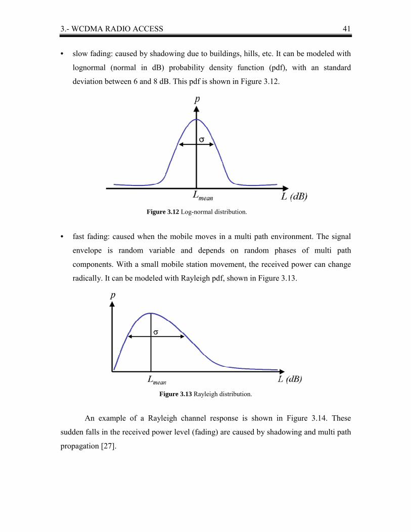
• slow fading: caused by shadowing due to buildings, hills, etc. It can be modeled with
lognormal (normal in dB) probability density function (pdf), with an standard
deviation between 6 and 8 dB. This pdf is shown in Figure 3.12.
Figure 3.12 Log-normal distribution.
• fast fading: caused when the mobile moves in a multi path environment. The signal
envelope is random variable and depends on random phases of multi path
components. With a small mobile station movement, the received power can change
radically. It can be modeled with Rayleigh pdf, shown in Figure 3.13.
Figure 3.13 Rayleigh distribution.
An example of a Rayleigh channel response is shown in Figure 3.14. These
sudden falls in the received power level (fading) are caused by shadowing and multi path
propagation [27].

3.- WCDMA RADIO ACCESS 42
Figure 3.14 Frequency response of Rayleigh channel.
4.- Angular spread: It describes the deviation of the signal incident angle. It can be
calculated in two planes, horizontal or vertical. The received power from the horizontal
plane is still the most important because of obstructing constructions: most of the
reflecting surfaces are related to the horizontal propagation and thus multiple BTS to MS
propagation paths exist more in the horizontal plane.
The horizontal angular spread is around 5-10 degree in macro cells and very wide
in microcellular and indoor environments because the reflecting surfaces surround the
base station antenna. The angular spread has a significant effect on antenna installation
direction and on the selection and implementation of traditional space diversity reception.
Vertical angular spread influences, additionally, the base station antenna array
tilting angle. The angular spread is also a key parameter when the performance of the
adaptive antennas is discussed because the optimization of the CIR depends strongly on
the incident angles of the carrier and on the interference signals. Thus, the performance of
the adaptive antennas is lower or more difficult to achieve in the microcellular
environments than in the macrocellular environments.

4.- PLANNING OF WCDMA RADIO NETWORKS 43
4.- PLANNING OF WCDMA RADIO NETWORKS
The UMTS deployment must be preceded by careful network planning. The
network planning tool must be capable of accurately modeling the system behaviour
when loaded with the expected traffic profile.
The WCDMA planning process can be divided into three phases which are initial
planning (dimensioning), detailed radio network planning and network operation, and,
finally, optimization. Each of these phases is studied in detail in this chapter. To
conclude, planned cell structure in UMTS cellular networks is analysed.
UMTS radio network planning is described in this chapter following the steps
indicated in [26] and in [28]. It is largely researched in those references.

4.- PLANNING OF WCDMA RADIO NETWORKS 44
4.1.- DIMENSIONING
The network planning tool should model the system behaviour with the expected
characteristics of the traffic. They describe the mixture of services being used by the
population of users. In order to accurately predict the radio coverage the system features
associated with WCDMA must be taken into account in the network modeling process.
In WCDMA network multiple services coexist. Different services (voice, data)
have different processing gains, Eb/N0 performance and thus different receiver SNR
requirements. In current 2nd generation systems´ coverage planning process the base
station sensitivity is constant and the coverage threshold is the same for each base station.
In the case of WCDMA the coverage threshold is dependent on the number of users and
used bit rates in all cells, thus it is cell and service specific.
Each phase of the WCDMA planning process, depicted in Figure 4.1 [28],
requires additional support functions like propagation measurements, key performance
indicator definitions, etc. In a cellular system where all the air interface connections
operate on the same carrier the number of simultaneous users is directly influencing on
the receivers´ noise floors. Therefore, in the case of UMTS the planning phases cannot be
separated into coverage and capacity planning, as in 2G system.
Initial planning (i.e. system dimensioning) provides the first and most rapid
evaluation of the network element count as well as the associated capacity of those
elements. This includes both the radio access network (UTRAN) as well as the core
network (CN). The target of the initial planning phase is to estimate the required site
density and site configurations for the area of interest. Initial planning activities include
knowledge of the size of the covered area, specification of the frequency band (for the
radio propagation characteristics), calculation of the path loss in both directions (from the
power budget, also called radio link budget), coverage analysis, capacity estimation, and
finally, estimation for the amount of base station hardware and sites, radio network
controllers (RNCs), equipment at different interfaces and CN elements. The service
distribution, traffic density, traffic growth estimates and QoS requirements are essential
already in the initial planning phase, when the quality is taken into account in terms of
blocking and coverage probability. Power budget calculation is done for each service (in

4.- PLANNING OF WCDMA RADIO NETWORKS 45
this work only speech service has been considered), and the tightest requirement shall
determine the maximum allowed isotropic path loss.
Figure 4.1 WCDMA radio network planning process.
If the radio network is new there have to be several scenarios on how to exceed
the coverage thresholds in different traffic situations. If an existing network is extended,
the traffic history over the area has to be used to identify traffic increases during the next
1-3 years.
The required number of base stations can be tuned by changing the base station
antenna height to correspond to the number accordingly based on traffic requirements for
the coverage area. Because traffic is increasing year after year, this analysis has to be
done based on differing traffic demands, with the final network configuration and
deployment strategy dependent on this long term analysis. If this long term analysis is not
done, the base station antennas will not be located correctly and the radio network
configuration will not be cost-efficient due to overcapacity or load and will require
continuous reconfigurations, which can not be avoided but they can be minimized.
Steadily increasing demands upon coverage cause changes, as in coverage thresholds,

4.- PLANNING OF WCDMA RADIO NETWORKS 46
and these changes have to be taken into account at the dimensioning stage because they
strongly influence base station site locations.
4.2.- DETAILED PLANNING
In the detailed planning phase the traffic distribution is used to allocate the
predicted traffic to the planned cells. This may lead to situations in which the load
between the cells can vary remarkably (some cells may have a load that is very close to
the maximum acceptable load and some cells may have a fairly low load). In this phase,
coverage targets are also checked.
All the cells are identical in the dimensioning phase but in the detailed planning
coverage predictions can be quite different between the cells due to propagation
environment and traffic distribution.
Detailed UMTS planning is divided in three phases which are configuration
planning, coverage predictions and topology planning (site configurations).
4.2.1.- Configuration Planning
Target in this phase is to estimate the maximum range of a cell. For this reason, a
power budget calculation is needed. In the power budget the antenna gains, cable losses,
diversity gains, fading margins, etc are taken into account. There are a few WCDMA
specific items in the link budget respect to the current TDMA based radio access system
like GSM.
The power budget is divided into five parts, which are general information,
service information, receiving end, transmitting end and isotropic path loss. The output of
the power budget calculation is the maximum allowed propagation path loss which in
return determines the cell range and thus the amount of sites needed.
General information of the power budget calculation is given in Table 4.1.

4.- PLANNING OF WCDMA RADIO NETWORKS 47
Parameter Value
Frequency [MHz] 2000
Chip rate [Mcps] 3.84
Reference temperature [K] 293
Boltzman´s constant [J/K] 1.38E-23
Table 4.1 General information of the power budget calculation.
Power budget is calculated for speech service (outdoor users with soft and softer
HO). Air interface bit rate for speech service is 15 Kbps in both directions, UL and DL.
Used load in the power budget calculation is in both directions, uplink and downlink,
75%. Data services have not been considered in this work.
Receiving end parameters are thermal noise density, interference degradation
margin, total noise power at the receiver, processing gain, required Eb/N0, receiver
sensitivity estimation, Low Noise Amplifier (LNA) gain, power control headroom or fast
fading margin and soft HO diversity gain.
Thermal noise density defines the noise floor due to thermal noise. When the
receiver noise figure is added, it is called noise power level at receiver and it is given by
[26]:
(Eq. 4.1)
where k is Boltzman´s constant, T0 is reference temperature in Kelvin, W is the CDMA
modulation bandwidth (3.84 MHz) and F is the noise figure of the receiver. It gives the
noise power in the case of an empty cell in watt.
The interference degradation margin is a function of the cell loading. The more
loading is allowed in the system, the larger interference margin is needed in uplink and
the smaller is the coverage area. Load in uplink direction is given by [28]:
(Eq. 4.2)
( )( )∑
=
++
=N
k
kkkb
UL i
RNEW1
0
11
1
α
η
WFkTPN 0=

4.- PLANNING OF WCDMA RADIO NETWORKS 48
where N is the total number of active users in a cell, (Eb/N0)k is the requirement of bit
energy to noise ratio for user k, R is user bit rate, α is user activity factor (voice activity)
and i is interference from other cells. It gives the load in %.
The downlink dimensioning is following the same logic as the uplink. For a
selected cell range the total base station transmit power ought to be estimated. In this
estimation the soft handover connections must be included. In the downlink equation
there is a new parameter called orthogonality, which shows the degree in which the users
in the same cell interfere with each other. With a orthogonality factor of 100% the users
do not cause interference for other users in the same cell [29]. If the power is exceeded
either the cell range ought to be limited or number of users in a cell has to be reduced.
Load in downlink direction is given by [26]:
(Eq. 4.3)
where ν is the orthogonality factor. Like the Eq. 4.2, it gives the load in %.
In the power budget calculation, in uplink direction the limiting factor is the
mobile station transmission power because it is much lower than the total base station
transmitted power. In downlink direction the limit is the total base station transmitted
power because of noise rise (transmission point-to-multipoint). When balancing the
uplink and downlink service areas both links must be considered.
The interference degradation margin to be taken into account in the power budget
due to a certain loading η (either in UL or DL) is [26]:
(Eq. 4.4)
where η is the load. It gives the interference degradation margin in dB. The load is always
compared to the maximum capacity of the cell (called pole capacity) so it is always in
between 0 % and 100%. Figure 4.2 shows that the interference degradation margin grows
towards infinity if load increases to 100%. In practice, when the interference degradation
margin is fixed, the maximum allowed load of the network is known.
( )η−−= 1log10 10L
( ) ( )[ ] k
N
kk
kbDL i
RW
NEανη ⋅+−=∑
=1
0 1

4.- PLANNING OF WCDMA RADIO NETWORKS 49
Figure 4.2 Interference degradation margin as a function of load.
Total noise power at the receiver is the noise floor including thermal noise, noise
generated by the receiver (noise figure) and interference.
Processing gain is the achieved gain due to spreading process and it is given by
Eq. 3.1.
Required Eb/N0 that is needed to be able to demodulate the signal shows ratio
between the received energy per bit and noise energy. It has to be selected based on the
service (speech or data).
In the link budget the BS receiver noise density is estimating the noise level over
one WCDMA carrier. The required receiver SNR contains the processing gain and the
loss due to the loading. The required signal power at the receiver, S, also called receiver
sensitivity, depends on the SNR requirement, receiver noise figure and system
bandwidth, and it is given by [28]:
(Eq. 4.5)
where [28]
(Eq. 4.6)
the noise power level at receiver, PN, is given by Eq. 4.1 and η is the load.
NPSNRS ⋅=
( ) ( )η−⋅=
10 WRNESNR b
4.- PLANNING OF WCDMA RADIO NETWORKS 50
Cable losses may cause limitations in the power budget in the UL direction,
especially when long cables are used. The UL direction can be improved by introducing a
Low Noise Amplifier (LNA) next to the receiving antenna. The LNA has to have a low
noise figure in order to improve the received field strength level at the base station
receiving end. The LNA has two important parameters when analysing its performance,
which are noise figure and gain. The target is to have as low a noise figure for the
amplifier as possible. Typical values are around 1.5 dB, which is almost the minimum
value. Gain due to LNA is typically 3.5-4 dB. The LNA also has an effect on the
performance of diversity reception because it depends on the received signal levels of the
main and diversity branches.
Power control headroom or fast fading margin is, as interference degradation
margin and soft HO diversity gain, a CDMA specific item in the power budget. Some
margin is needed in the mobile station transmission power for maintaining closed loop
fast power control in unfortunate propagation conditions like the cell edge. This is
applicable especially for pedestrian users where the Eb/N0 to be maintained is more
sensitive to the closed loop power control. It has been studied more in [30-31].
Handovers provide gain against shadow fading by reducing the required fading
margin. By making handovers, the mobile can select a better communication link.
Furthermore, soft HO (macro diversity) gives and additional gain against fast fading by
reducing the required Eb/N0 relative to a single radio link. The amount of gain is a
function of mobile speed, diversity combining algorithm used in the receiver and power
delay profile of the radio channel and it consists of two parts: this above mentioned gain
against fast fading and gain against slow fading.
Transmitting end in the WCDMA power budget is similar to current GSM power
budget. But there are two main differences. First is that BTS power is given per user in
WCDMA (in GSM one user gets the full transmission power when using the time slot
while in WCDMA the output power of a BTS is shared between the control channel and
all the users in a sector/cell. For this reason, if a user could use the full power of a
WCDMA base station this would mean that there cannot be other users in that sector/cell
at that moment) and second is that in WCDMA base stations there is a different

4.- PLANNING OF WCDMA RADIO NETWORKS 51
combining respect to GSM thus there are no combiner loss in the WCDMA power
budget.
The next step is to estimate the maximum cell range and cell coverage area in
different environments/regions. The power budget is estimating the maximum allowed
isotropic path loss, which is calculated in the same way as it is for a GSM cell. In
WCDMA power budget there can be remarkable differences in isotropic path losses
between UL and DL, basically due to asymmetry in traffic (especially in packet data) and
possible different bit rates in the UL and DL. Then, the isotropic path loss is used for cell
range calculations in a similar way as it is used in GSM.
WCDMA power budget in simulations is calculated in Table 4.2.
Parameter UL DL
Thermal noise [dBm] -108.15 -108.15 A
RX noise figure [dB] 5 9 B
Noise power at receiver [dBm] -103.15 -99.15 C=A+B
Interference margin [dB] 6.02 6.02 D
Total noise power at receiver [dBm] -97.13 -93.13 E=C+D
Processing gain [dB] 24.08 24.08 F
Required Eb/N0 [dB] 5 8 G
RX sensitivity [dBm] -116.21 -109.21 H=E-F+G
RX antenna gain [dB] 18 0 I
Cable loss / Body loss [dB] 2.5 3 J
LNA gain [dB] 4 0 K
Soft HO diversity gain [dB] 1.5 3 L
Power control headroom [dB] 2 2 M
Required signal level [dBm] -135.21 -107.21 N=H-I+J-K-L+M
TX power [dBm] 21 33 O
Cable loss / Body loss [dB] 3 2.5 P
TX antenna gain [dBi] 0 18 Q
Peak EIRP [dBm] 18 48.5 R=O-P+Q
Allowed propagation loss [dB] 153.21 155.71 S=-N+R
Table 4.2 WCDMA power budget in simulations.
4.- PLANNING OF WCDMA RADIO NETWORKS 52
( ) [ ]( ) ( ) ( )( ) [ ]( ) KkmsdhChMHzfBAdBL bb −⋅−+−+= loglog55.6log82.13log
4.2.2.- Coverage Predictions
Next step is to estimate the coverage probability. This means that the standard
deviation for the log-normal fading and the propagation model exponent (according to the
values given in Table 3.2) must be set.
In the indoor case, the indoor loss is from 15 to 18 dB and the standard deviation
for log-normal fading margin calculation is set to 10-12 dB. In the outdoor case, typical
standard deviation value is 7 to 10 dB.
In real WCDMA cellular networks the coverage areas of cells overlap and the
mobile station is able to connect to more than just one serving cell. If more than one cell
can be detected the location probability increases and is higher than determined for a
single isolated cell.
In macro cells the base station is usually above rooftops and it is not possible to
calculate analytically the signal strength because of very complex propagation media.
Therefore, the empirical or semi empirical propagation models should be used. Once the
maximum allowed propagation loss in a cell is known, it is easy to apply any known
propagation model for the cell range estimation. The propagation model should be chosen
so that it optimum describes the propagation conditions in the area. The restrictions of the
model are related to the distance from the base station, the base station effective antenna
height, the mobile antenna height and the frequency. One typical example for macro
cellular environment is Okumura-Hata which is a empirical propagation model.
The Okumura-Hata model is widely used for coverage prediction in macro cells.
Based on measurement data made by Okumura in Tokyo in 1968, this data set was fitted
to mathematical model by Hata in 1980. Basic model was made for urban areas but
additionally correction factors for suburban areas and rural areas, irregular terrains and
for different base station and mobile station antenna heights have been applied. This
model is not applicable when the base station antenna is below rooftops.
The Okumura-Hata model can be written as shown in Eq. 4.7 [24].
llll(Eq. 4.7)
according to the values given in Table 4.3.

4.- PLANNING OF WCDMA RADIO NETWORKS 53
Value at frequency between 150 MHz and 1 GHz
Value at frequency between 1.5 and 2 GHz
A 69.55 46.30 B 26.16 33.90
Table 4.3 Okumura-Hata model parameters as a function of frequency. where hb is the base station antenna height in meters, d is the link distance in kilometers, f
is the center frequency in MHz, C is a tunable parameter which depends on propagation
environment (44.9 as a default value but it can vary between 44 and 47) and, finally, K is
an addition correction factor due to topology or morphology which has 0 as a default
value.
Figure 4.3 shows an example of path loss as a function of distance, by using
Okumura-Hata model [24].
Figure 4.3 Path loss as a function of distance by using Okumura-Hata model.
Eq. 4.8 presents an example of Okumura-Hata path loss model for an urban macro
cell with base station antenna height of 25 meters and carrier frequency of 2000 MHz.
More about this has been studied in [32].
(Eq. 4.8)
( ) [ ]( )kmsrdBL log7.359.138 ⋅+=

4.- PLANNING OF WCDMA RADIO NETWORKS 54
Table 4.4 shows typical maximum allowed path loss of existing GSM and
WCDMA systems.
GSM 900
GSM 1800
WCDMA
speech
WCDMA
64 Kbps
WCDMA
144 Kbps
Maximum path loss [dB] 160 154 156 157 154
Table 4.4 Typical maximum allowed path loss of existing GSM and WCDMA systems.
According to the power budget calculation (see Table 4.2) maximum allowed path
loss is 153.21 dB. Slow fading margin (which is typically 10 dB) has to be considered in
the cell range calculation and it should be subtracted from the maximum allowed path
loss before using Eq. 4.8. According to this, cell range cannot be more than 1.3 kms.
After choosing the cell range the coverage area can be calculated. The coverage
area for one cell in hexagonal configuration can be calculated with [28]:
(Eq. 4.9)
where S is the coverage area, r is the maximum cell range and K is a constant, depending
on the network topology. Its value changes according to the site configuration, as shown
in Table 4.5.
SITE CONFIGURATION onmi. 2-sectored 3-sectored 6-sectored
K 2.6 1.3 1.95 2.6
Table 4.5 K-values for the site area calculation.
According to the example given in Eq. 4.8, coverage area by using 6-sectored
sites is 4.4 km2/cell (26.4 km2/site). Total coverage area when 19 base stations are placed
is 500 km2, which is approximately the land area of Tampere. Large variations of this
calculated value due to, for example, coverage overlapping should be taken into account
in real implementation (if even small amount of coverage overlapping, theoretical total
coverage area, this 500 km2, will decrease heavily). For this reason, accurate choices for
those parameters concerning to the topology of the network, like antenna beamwidth, are
key technical elements in topology planning, which is explained in detail in section 4.2.3.
2rKS ⋅=

4.- PLANNING OF WCDMA RADIO NETWORKS 55
Once the site coverage area is known the site configurations in terms of channel
elements, sectors and carriers has to be selected so that the supported traffic density can
fulfil the requirements.
Special emphasis has to be given to the consideration of mutual influence of
coverage and capacity (as indicated in Figure 4.4) [29]. As it has been said before, the
coverage is limited by the uplink because of the maximum available transmission power
of the mobile while the downlink sets limitations on the capacity due to the increasing
interference level [33-34].
Figure 4.4 Mutual influence of coverage and capacity in WCDMA networks.
For this reason, in the very beginning the operator should have knowledge and
vision of the subscriber distribution and growth since it has a direct impact on the
coverage. Finding the correct configuration for the network so that the traffic
requirements are met and the network cost minimized is not a simple task: the number of
carriers, sectoring, loading, number of users and cell range all have a great impact on the
final result.
As coverage and capacity depend on the instantaneous traffic distribution and
influence each another, a simulation combining the uplink and downlink analysis in an
adequate way is required. Figure 4.5 shows how this influence affects the network design
and how this process can be done.

4.- PLANNING OF WCDMA RADIO NETWORKS 56
Figure 4.5 Impact of coverage and capacity on WCDMA network design.
The evaluation of the optimized base station locations can be done when the
planning threshold is defined. It means that the reasonable QoS level for the different
geographical locations have to be agreed: first major national areas, cities and roads
where coverage has to exist and then subareas of them such as urban and suburban areas.
The planning threshold also concerns whether the service has to be extended inside
vehicles and buildings in different areas.
The planning threshold itself is defined as in the GSM by starting from the mobile
station sensitivity (threshold is for the DL direction) and by adding the required planning
margins to the sensitivity level. The required margins in the WCDMA system are:
• slow fading margin (shadowing)
• macro diversity or soft HO gain
• power control headroom (fast fading margin)
• body loss
• antenna orientation loss
• in-vehicle or indoor penetration loss
• interference margin
The planning threshold is calculated by adding all these components to the mobile
station sensitivity.

4.- PLANNING OF WCDMA RADIO NETWORKS 57
4.2.3.- Topology Planning
As is has been said, coverage and capacity planning of UMTS WCDMA cellular
networks cannot be separated, since they are connected to each other. Topology planning
in 3rd generation networks combines coverage and capacity planning which contains
definition of site locations and configuration together with base station antenna
configuration, since these elements influence much on the service coverage and system
capacity of the UMTS network.
Service coverage and system capacity together with sufficient QoS and
economical implementation costs are the most essential factors that determine an
operator´s site density and site configuration for a given planning area. Site densities and
configuration of a UMTS network mainly determine coverage and capacity of a site. In
urban environments, the traffic requirements are much higher than in rural areas and thus
the site density and configuration is different for these cases. Moreover, used
implementation strategy for site configuration defines the over all coverage and capacity
of that particular site. Site locations, the number of sectors and their directions together
with antenna configuration have to be considered in such a manner that given service
coverage, system capacity and QoS requirements are satisfied with reasonable
implementation costs.
Coverage and capacity planning are linked together via power budget calculation
and load equations. This phenomenon makes it impossible to handle coverage and
capacity separately. Because of coverage depends on the loading of the network, system
level simulations are needed in order to determine the performance of UMTS network in
different planning scenarios.
The capacity of UMTS network is known to be interference limited, i.e. soft
capacity limited. For these systems, the Erlang capacity cannot be directly calculated
from Erlang-B formula, since it would give too pessimistic results. It over-estimates the
capacity need since each service is handled alone in the system calculations. If the system
is code limited, the capacity can be estimated from Erlang-B model. In code limited
situation the noise rise in the network is not causing outage or blocking, since the
communication between links is limited by the number of codes. Hence, in code limited

4.- PLANNING OF WCDMA RADIO NETWORKS 58
situation the behaviour of WCDMA network is like FDMA/TDMA based systems and
therefore Erlang-B formulas can be used. In noise limited situations the communication is
limited due to noise rise of the system, not due to the available number of codes.
In contrast to GSM networks, the capacity of UMTS network is said to be soft
blocked. In soft blocked networks the interference rise in a cell causes the blocked calls
instead of the blocking would be caused by the lack of available traffic channels or in
case of UMTS available number of codes.
Main elements in UMTS topology planning are sectoring, antenna beamwidth,
site separation, antenna height and tilting.
The term sectoring refers to increasing the number of sectors belonging to a site
[35]. In existing cellular networks, 3-sectored sites are commonly used. It has been
proposed and researched in many papers that even higher sectoring order, like 6-sectored
sites, would bring coverage and capacity enhancements for UMTS networks.
Omnidirectional base station antennas are typically used in small micro cells or
in indoor cells. Two-sectored base stations are used mainly in sectored micro cells or to
provide roadside coverage. Standard macrocellular solution for low or average loaded
networks would be use of 3-sectored sites and in macrocellular environment for high
capacity needs, 6-sectored sites would provide the best solution.
Sectoring is used in UMTS system to increase the system capacity as well as the
service coverage. It seems to be intuitive that adding more antennas to base station site
configuration increases the capacity of the site. Increasing number of sectors at the base
station site requires also place for addition hardware: when the number of sectors is
doubled, the amount of hardware is also doubled.
The effect of sectoring has two perspectives: if widebeam antennas are used,
coverage threshold is better but the interference level is also higher. Three and six-
sectored sites are depicted in Figure 4.6.

4.- PLANNING OF WCDMA RADIO NETWORKS 59
Figure 4.6 Cell structure for three and six sectors/site. Base station antenna beamwidth plays an important role in UMTS network
performance. With proper antenna beamwidth, especially the number of softer HO
connections can be controlled. Figure 4.7 shows the effect of the antenna beamwidth over
sector overlapping.
Figure 4.7 Coverage vs interference level.
Overlapped areas are possible softer HO areas, which are needed in UMTS
network in order to maintain the interference level as low as possible during sector HO
procedure. But too large softer HO areas consumes limited radio resources of the base
station. Wider base station antenna beamwidth also increases the interference level of the

4.- PLANNING OF WCDMA RADIO NETWORKS 60
neighbouring sector and thus reduces the capacity. The importance of base station
antenna beamwidth is emphasized in higher sectoring order [36].
Site separation is another key element of UMTS topology planning. Having sites
close to each other (big overlap between the cell sites) means that achieved coverage is
good in indoor as well as in outdoor locations. Conversely, this means also higher
interference levels in the network and decreased capacity values [37]. The capacity also
decreases due to higher number of soft HO connections. When the base stations are
placed far apart the cell ranges belong too long and this situation yields for high
transmission power for the mobiles located near the cell edges. Thus, the amount of
coverage overlapping is always on optimization tasks and a trade of between coverage
and capacity requirements.
Base station antenna height affects on the propagation signal near the base station
antenna. Until certain distance, the propagation near the base station antenna happens
with propagation slope of 20 dB/dec. This distance where the propagation slope changes
is called breakpoint distance. After this point, the propagation slope is determined by the
environment.
Use of higher antenna positions yields for larger coverage areas but also for
higher interference levels for surrounding cells [38]. Without tilting the base station
antenna, the interference level of the neighbouring cells increases and the capacity
decreases.
Antenna tilt is a key parameter in controlling interference and it is used, either in a
mechanical way or in an electrical manner, in order to minimize the ratio of interference
[39]. Tilt also affects the throughput at a site, making it a key differentiator when it
comes to QoS. Changing the elevation pattern offers a great opportunity for optimization.
Antenna tilt has not been used in this work.
When one of these elements is changed, the performance of the system is also
changing: sector overlapping grows with antenna height and antenna beamwidth and
when higher site separation is used the interference level between cells is lower but path
loss is higher. These are only some examples about how those parameters concerning to
the topology of the network are affecting to the system performance. More about that can
be found in [40].

4.- PLANNING OF WCDMA RADIO NETWORKS 61
Used values in simulations for those key elements of the topology planning are
shown in Table 4.6. These values have been chosen because of typical macro cellular
network layout and configuration are used. As it has been said, antenna tilt has not been
used in this work.
ANTENNA
BEAMWIDTH
[degree]
SITE
SEPARATION
[kilometers]
ANTENNA
HEIGHT
[meters]
3-SECTOR CASE 65 – 90 1.5 – 2.0 – 2.5 25 – 45
6-SECTOR CASE 33 – 65 1.5 – 2.0 – 2.5 25 – 45
Table 4.6 Simulation values of the network topology parameters.
Simulations will combine all these values in two different scenarios (three and six
sectors/site) and the objective will be to study their impact on capacity in the designed
WCDMA network. .
4.3.- OPTIMIZATION
WCDMA system needs, like GSM, continuous monitoring because the mobile
users´ location and traffic behaviour varies all the time. This monitoring requirement is
only emphasized in the WCDMA because the traffic demand can vary strongly and this
variation influences directly the radio network quality. The better and more accurately the
traffic amount and locations can be modelled the better and more efficiently the radio
network can be designed and implemented.
Main indicators that should be monitored are traffic, soft HO percentage, average
transmitted and received power, drop calls, handovers per call and per cell, throughput
and BER [26].
4.4.- CELL TYPES
For optimal UMTS performance, it is proposed that UMTS network is planned by
using a hierarchical cell structure (HCS): macro, micro and pico cells [41-43]. In general,
QoS and capacity requirements need to be guaranteed in the smallest cells, which are the
most critical cells. A possible use of the hierarchical cell structure is shown in Figure 4.8.

4.- PLANNING OF WCDMA RADIO NETWORKS 62
Figure 4.8 A hierarchical cell scenario in UMTS.
Large cells guarantee a continuous coverage for fast moving mobiles while small
cells are necessary to achieve good spectrum efficiency and high capacity for hot spot
areas. With flexible deployment, it could be possible for an operator to redeploy pico cell
channels for macro cells outside of urban cells in some locations.
The FDD macro cellular network provides a wide area of coverage and it is used
for high speed movement mobiles. Micro cells are used at street level for outdoor
coverage to provide extra capacity where macro cells could not scope. Those micro cells
would not be hexagonal in shape but rather canyonlike, reflecting the topography of a
street and be typically 200 - 400 m in distance. Pico cells would be deployed mainly in
indoor areas where there is a demand for high data rate services such as laptops
networking or multimedia conferencing. Such cells may be in the order of 50 m (typical
value) in distance. A limiting factor will be the range of these terminals when used for
high data rate services. Maximum bit rate for macro cells is hoped to be 384 Kbps and
until 2 Mbps for pico cells.
Main characteristics of these cell types, which are summarized in Table 4.7, are as
follows:

4.- PLANNING OF WCDMA RADIO NETWORKS 63
MACRO CELLS
• Cell range >1 km
• High transmission powers (>10 Watt)
• High gain, directive antennas (Ga = 10 - 20 dB)
• Data rates until 384 Kbps
• Basic coverage and capacity over large area in the first phase of network roll-out
• Low isolation between cells
• High delay spread, fast moving mobiles
• Propagation phenomena very difficult to compute analytically
• Many different propagation paths
• Lots of scattering
MICRO CELLS
• Cell range 100 m to 1 km
• Medium to high transmission powers (>1Watt)
• BS cabinet can be outdoors or indoors (long cabling in some cases)
• Medium gain antennas (Ga = 5 - 10 dB, θ3dB = 60 � 120 degree)
• Data rates even higher than 384 Kbps
• Hot-spot capacity and continuous micro coverage in some cases
• Both outdoor and indoor coverage
• Good isolation between adjacent cells
� buildings isolate cells
� good spectral efficiency
• Low minimum coupling loss close to antenna (50 - 60 dB)
• Low delay spread: only few strong propagation paths
• LOS propagation: line of sight

4.- PLANNING OF WCDMA RADIO NETWORKS 64
• Street corner effect:
� when the mobile moves from
LOS to NLOS the signal strength
might drop 20 - 30 dB
� fast moving mobiles are problematic
• Very high site density up to 20 - 30 sites per km2
PICO CELLS
• Cell range from 10 m to 100 m
• Two solutions: pico BS or distributed antenna systems (DAS)
• Small (pico BS) to high (DAS) transmission powers
• Low gain antennas (Ga = 2 dB)
• Data rates until 2 Mbps
• Hot-spot capacity / indoor coverage
• Problems:
� interaction with outdoor cells: power leaking
� low isolation
� different powers
• Low minimum coupling loss (35 - 50 dB)
• Very low delay spread: only few strong propagation paths → low multi path diversity
and good orthogonality
• Application areas: offices, shopping malls, railway stations, airports, hotels�
CELL TYPE RANGE APPLICATION
Umbrella cells Up to several hundred of
Kms.
Satellite mobile Filling supply gaps
Support traffic peaks Hyper cells > 20 kms. Rural areas Macro cells 1 km. – 20 kms. Highways and suburban areas Micro cells 100 m. – 1 km. Cities and urban areas Pico cells < 100 m. In-building (offices, hotels, etc)
Table 4.7 Ranges and applications of the different UMTS cell types.

5.- SIMULATIONS 65
5.- SIMULATIONS
In this chapter the simulator is presented, including its characteristics and how is
it working. After this, simulations results are depicted, classified by number of sectors
used in the sectoring process. Finally, the best configurations for both cases of sectoring
are compared in order to know the best shape for our design.

5.- SIMULATIONS 66
5.1.- SIMULATION SETUP
Nokia´s simulator NetAct WCDMA Planner 4.0 is used in its static simulation
type. Static simulation is a method where the performance of the network is analysed
over various instances in time or snapshots, where User Equipments (UEs) are in
statistically determined places. The ability of each terminal to make its connection to the
network is calculated through an iterative process.
Various failure mechanisms are typically considered, such us maximum mobile
transmission power, maximum Node B power reached, no available channels or low pilot
Ec/Io.
The performance of the network is then analysed from the results of the snapshots
carried out. Monte-Carlo analysis has been used in this thesis as used in WCDMA
Planner. It is a form of static simulation which requires hours of computing time.
NetAct WCDMA Planner 4.0 offers also the possibility of run dynamic
simulations. In those simulations, UEs moving through the network in successive time
steps are simulated. A mobile list is generated and solved for the first time step. The
simulation may consider time to be split into chip periods, bit periods and time steps
(SNR considered). Successive time steps are then simulated and are dependent upon the
results of the previous time slot. New mobiles are simulated coming into the network and
terminating their calls.
Main advantages and disadvantages of these WCDMA simulation methods are
shown in Table 5.1
Method Accuracy Complexity Taken time
Static calculation
Not very accurate,
particularly with
global margins
Relatively
straightforward to
use once
configured
Shortest
Static simulation
Reasonable but
does not deal with
dynamic network
performance
More difficult to
configure and gives
more complicated
results
Moderate
depending on the
number of UEs
and calls
Table 5.1 Advantages and disadvantages of WCDMA simulation methods.

5.- SIMULATIONS 67
Method Accuracy Complexity Taken time
Dynamic
simulation
Quite high
assuming no bad
assumptions are
made to speed it
up
Difficult to judge
results
Extremely long if
multiple runs are
performed for
statistical validity
Table 5.1 (cont.) Advantages and disadvantages of WCDMA simulation methods.
What is Monte-Carlo simulation? Traditionally, TDMA/FDMA network planning
used static analysis and calculated the margins for a tuned propagation model in order to
protect the system of interferences. Gains were applied to allow for the soft handover
technique. However, as the level of intra cell and inter cell interference varies between
cells, this approach gave misleading results in early networks. Thus, in CDMA networks,
coverage and cell capacity are too interrelated to be predicted accurately with static
analysis to derive margins and gains.
An alternative approach has developed based around simulating networks by
using Monte-Carlo algorithms. Existent WCDMA Planner in NetAct WCDMA Planner
4.0 uses this approach as it provides a good balance between accuracy and usability.
A large number of randomized snapshots are taken of the network performance
for different UEs or terminals over time. In these snapshots, the UEs are in statistically
determined positions and generated independently for each snapshot.
The number of terminals in an active session in a pixel is determined by using a
Poisson distribution with a mean given by the number of terminals in the traffic array.
This means that the total number of terminals in a snapshot is Poisson distributed and so
it will vary from snapshot to snapshot.
These snapshots are then used in calculations to obtain statistically valid
measurements giving an estimate of the mean network performance.
An advantage of using the static Monte-Carlo simulation approach is that it takes
less time than dynamic simulation (where you look at mobiles moving through the
network). Repeated static simulation proves its value for detailed optimization of site
configurations, problem areas and radio resource management algorithms.

5.- SIMULATIONS 68
Used simulation environment is given by a digital map of Tampere area, which is
a city similar to Tarragona in Spain (number of people, geography and other
characteristics are quite the same).
Nineteen base stations (the first two interfering tiers and the central base station)
in hexagonal grid are placed in Tampere area in order to provide UMTS speech service to
the city. Figure 5.1 shows the digital map of Tampere used in the simulations and these
nineteen base stations in the case where three sectors/site have been used. The hexagon
limits the simulation area, so there are terminals only inside it.
Figure 5.1 Digital map of the simulation area.
The simulator needs as inputs a digital map, the network layout, where are
defined the number of sectors/site and the cell range; the traffic raster, which contains the
mobile distribution in the network and many other parameters which are needed by the
Monte-Carlo simulation and, finally, the site configuration, where the antenna parameters
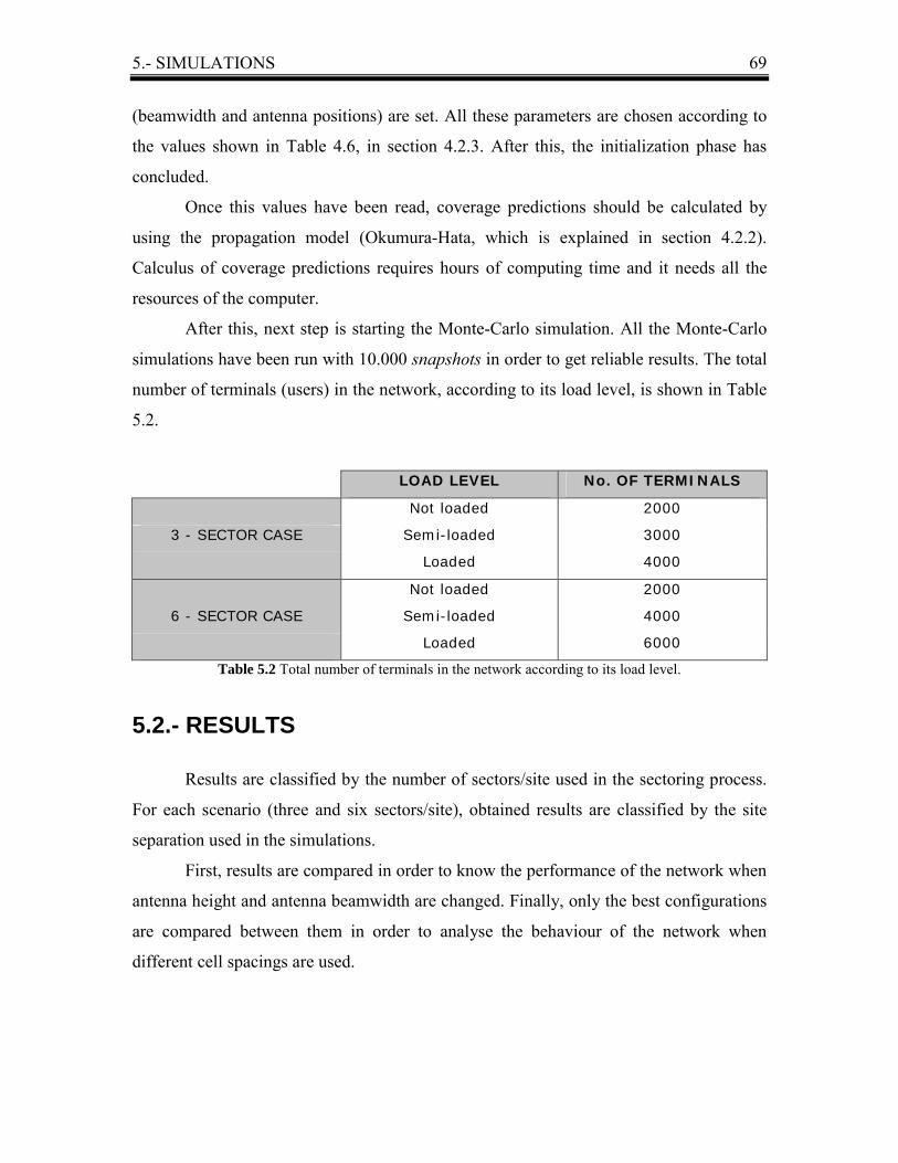
5.- SIMULATIONS 69
(beamwidth and antenna positions) are set. All these parameters are chosen according to
the values shown in Table 4.6, in section 4.2.3. After this, the initialization phase has
concluded.
Once this values have been read, coverage predictions should be calculated by
using the propagation model (Okumura-Hata, which is explained in section 4.2.2).
Calculus of coverage predictions requires hours of computing time and it needs all the
resources of the computer.
After this, next step is starting the Monte-Carlo simulation. All the Monte-Carlo
simulations have been run with 10.000 snapshots in order to get reliable results. The total
number of terminals (users) in the network, according to its load level, is shown in Table
5.2.
LOAD LEVEL No. OF TERMINALS
Not loaded 2000
3 - SECTOR CASE Semi-loaded 3000
Loaded 4000
Not loaded 2000
6 - SECTOR CASE Semi-loaded 4000
Loaded 6000
Table 5.2 Total number of terminals in the network according to its load level.
5.2.- RESULTS
Results are classified by the number of sectors/site used in the sectoring process.
For each scenario (three and six sectors/site), obtained results are classified by the site
separation used in the simulations.
First, results are compared in order to know the performance of the network when
antenna height and antenna beamwidth are changed. Finally, only the best configurations
are compared between them in order to analyse the behaviour of the network when
different cell spacings are used.

5.- SIMULATIONS 70
5.2.1.- Scenario 1: 3-Sector Case
3-SECTORED SITES OF 1.5 km.
2000 T 3000 T 4000 T
90 degree / 25 m
Service probability [%] 100 96.9 79.6Mean # of mobiles in soft HO [%] 19.6 19.3 20.5Mean # of mobiles in softer HO [%] 12 12 13Uplink load [%] 42 61.3 67.2Other-to-own cell interference 0.94 0.942 0.914DL TX. power [dBm] 35.2 38.6 40.4Throughput [kbps/sector] 289.6 420.9 469.1Noise rise [dB] 2.39 4.18 4.88
90 degree / 45 m
Service probability [%] 97.7 79.6 55.7Mean # of mobiles in soft HO [%] 38.1 40.6 43.3Mean # of mobiles in softer HO [%] 9.6 10.5 11.4Uplink load [%] 53.5 63.6 58.8Other-to-own cell interference 1.535 1.48 1.43DL TX. power [dBm] 37.5 40.2 41.3Throughput [kbps/sector] 336.6 415.7 394.9Noise rise [dB] 3.4 4.43 3.89
65 degree / 25 m
Service probability [%] 100 98.7 86.1Mean # of mobiles in soft HO [%] 18.9 18.5 19.1Mean # of mobiles in softer HO [%] 4.8 4.7 5Uplink load [%] 38.6 57.3 66.4Other-to-own cell interference 0.744 0.751 0.729DL TX. power [dBm] 34.6 37.8 39.7Throughput [kbps/sector] 271.9 401.4 470.5Noise rise [dB] 2.14 3.77 4.81
65 degree / 45 m
Service probability [%] 98.8 86.7 65.1Mean # of mobiles in soft HO [%] 33.5 34.9 37.6Mean # of mobiles in softer HO [%] 3.7 4 4.4Uplink load [%] 48.7 62.8 62.6Other-to-own cell interference 1.212 1.188 1.153DL TX. power [dBm] 36.5 39.6 40.9Throughput [kbps/sector] 312.7 412.6 421.8Noise rise [dB] 2.97 4.385 4.32
Figure 5.2 Results of 3-sectored sites, 1.5 km. site separation.
In this case, base stations are close to each other. For this reason the interference
level is increasing quickly if wide and/or high antennas are used (degrading too much the
service probability when the network is loaded). According to the results shown in Figure
5.2, the best antenna configuration is 65 degree antenna beamwidth and 25 meters of
antenna height. Because of the distance between base stations is small, coverage is good
and this antenna configuration supplies a good interference level.

5.- SIMULATIONS 71
Figure 5.3 shows sector throughput as a function of DL traffic power for different
antenna configurations.
250
300
350
400
450
500
34 35 36 37 38 39 40 41 42
DL. AVERAGE TRAFFIC POWER [dBm]
SEC
TOR
TH
RO
UG
HPU
T [K
bps/
sect
or]
90_25
90_45
65_25
65_45
Figure 5.3 Sector throughput vs downlink traffic power with 3-sectored sites, 1.5 km. site separation.
When the transmitted power exceeds 40 dBm, the network starts to be saturated in
all cases, except for the best configuration (65_25), where the saturation area begins later.
Following the same tendency, Figure 5.4 shows the service probability as a function of
sector throughput, also for the different antenna configurations.
75
80
85
90
95
100
250 300 350 400 450 500
SECTOR THROUGHPUT [Kbps/sector]
SER
VIC
E PR
OB
AB
ILIT
Y [%
]
90_2590_4565_2565_45
Figure 5.4 Service probability vs sector throughput with 3-sectored sites, 1.5 km. site separation.

5.- SIMULATIONS 72
3-SECTORED SITES OF 2.0 km.
2000 T 3000 T 4000 T
90 degree / 25 m
Service probability [%] 99.7 96.9 82.7Mean # of mobiles in soft HO [%] 16.1 15.8 16.2Mean # of mobiles in softer HO [%] 12.4 12.3 13.1Uplink load [%] 39.4 57.8 65.5Other-to-own cell interference 0.824 0.833 0.798DL TX. power [dBm] 34.9 38.1 39.8Throughput [kbps/sector] 281.3 409.5 471Noise rise [dB] 2.22 3.84 4.7
90 degree / 45 m
Service probability [%] 99.9 93.3 69.7Mean # of mobiles in soft HO [%] 26.6 26.8 29.1Mean # of mobiles in softer HO [%] 11.9 12.2 13.6Uplink load [%] 46 64.5 64.5Other-to-own cell interference 1.131 1.128 1.086DL TX. power [dBm] 36.1 39.6 41Throughput [kbps/sector] 309.8 435.6 445.3Noise rise [dB] 2.71 4.55 4.53
65 degree / 25 m
Service probability [%] 99.6 98.5 87.8Mean # of mobiles in soft HO [%] 16.5 16 16.2Mean # of mobiles in softer HO [%] 5.1 5 5.2Uplink load [%] 36.3 53.9 63.8Other-to-own cell interference 0.645 0.658 0.63DL TX. power [dBm] 34.3 37.4 39.2Throughput [kbps/sector] 266.7 394 469.6Noise rise [dB] 2 3.47 4.52
65 degree / 45 m
Service probability [%] 99.9 97.1 79.5Mean # of mobiles in soft HO [%] 25.5 25.2 26.4Mean # of mobiles in softer HO [%] 4.4 4.3 4.7Uplink load [%] 42.2 61.4 66.7Other-to-own cell interference 0.901 0.908 0.875DL TX. power [dBm] 35.4 38.8 40.3Throughput [kbps/sector] 289.8 421.4 465.4Noise rise [dB] 2.41 4.22 4.83
Figure 5.5 Results of 3-sectored sites, 2.0 km. site separation.
This configuration is, according to the results shown in Figure 5.5, a medium case
and use of wide and high antennas is now better supported, compared to sites of 1.5
kilometers, because the degradation of the service probability, which is caused by this
use, is not so important, except in the worst case (wide and high antennas). The best
antenna configuration is still 65 degree and 25 meters. This configuration gives better
results in both aspects: service probability and capacity, especially when the network is
loaded.

5.- SIMULATIONS 73
Figure 5.6 shows sector throughput as a function of DL traffic power for different
antenna configurations.
250
300
350
400
450
500
550
34 35 36 37 38 39 40 41 42
DL. AVERAGE TRAFFIC POWER [dBm ]
SEC
TOR
TH
RO
UG
HPU
T [K
bps/
sect
or]
90_25
90_45
65_25
65_45
Figure 5.6 Sector throughput vs downlink traffic power with 3-sectored sites, 2.0 km. site separation.
The same effect appears again: when the transmitted power exceeds 40 dBm, the
network starts to be saturated but this time also for the best configuration. Figure 5.7
shows the service probability, much better compared to sites of 1.5 kilometers (especially
in the worst cases: 65_45 and 90_45) as a function of sector throughput.
75
80
85
90
95
100
250 300 350 400 450 500
SECTOR THROUGHPUT [Kbps/sector]
SER
VIC
E PR
OB
AB
ILIT
Y [%
]
90_25
90_45
65_25
65_45
Figure 5.7 Service probability vs sector throughput with 3-sectored sites, 2.0 km. site separation.
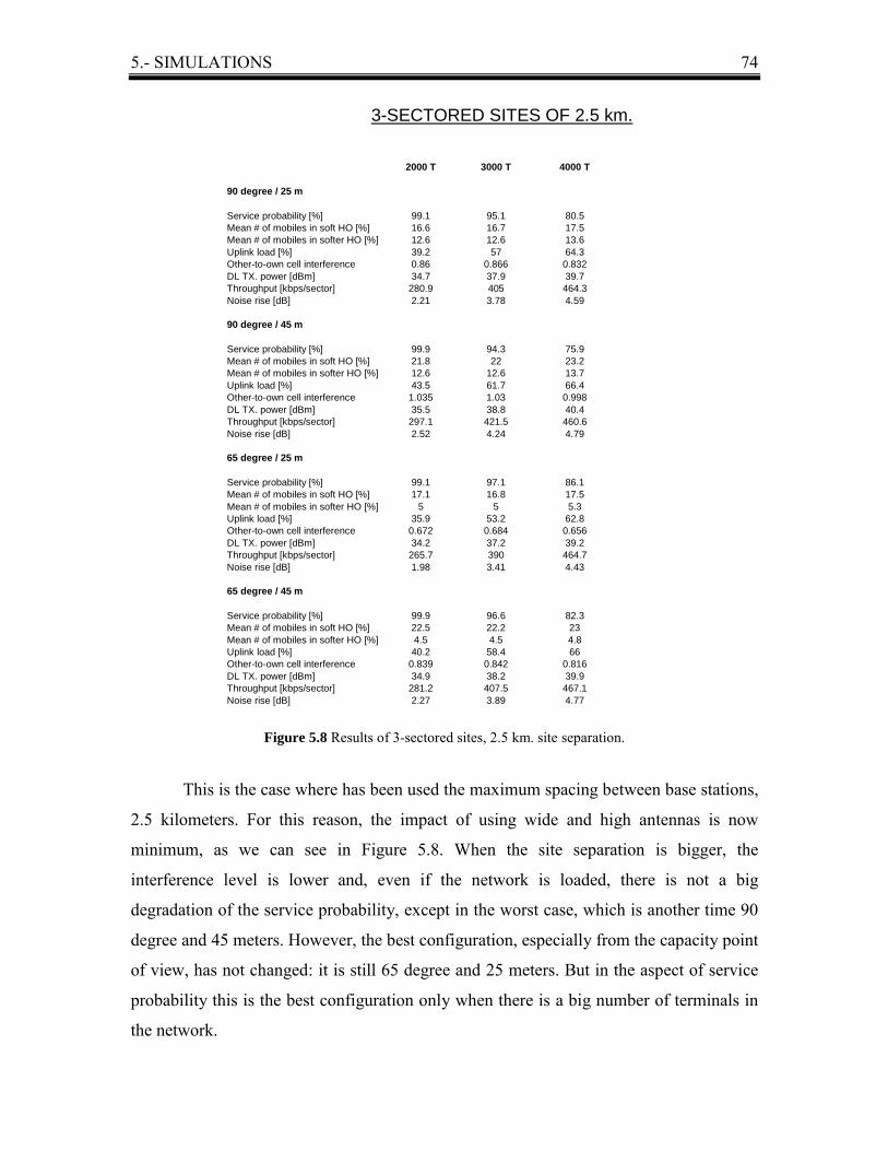
5.- SIMULATIONS 74
3-SECTORED SITES OF 2.5 km.
2000 T 3000 T 4000 T
90 degree / 25 m
Service probability [%] 99.1 95.1 80.5Mean # of mobiles in soft HO [%] 16.6 16.7 17.5Mean # of mobiles in softer HO [%] 12.6 12.6 13.6Uplink load [%] 39.2 57 64.3Other-to-own cell interference 0.86 0.866 0.832DL TX. power [dBm] 34.7 37.9 39.7Throughput [kbps/sector] 280.9 405 464.3Noise rise [dB] 2.21 3.78 4.59
90 degree / 45 m
Service probability [%] 99.9 94.3 75.9Mean # of mobiles in soft HO [%] 21.8 22 23.2Mean # of mobiles in softer HO [%] 12.6 12.6 13.7Uplink load [%] 43.5 61.7 66.4Other-to-own cell interference 1.035 1.03 0.998DL TX. power [dBm] 35.5 38.8 40.4Throughput [kbps/sector] 297.1 421.5 460.6Noise rise [dB] 2.52 4.24 4.79
65 degree / 25 m
Service probability [%] 99.1 97.1 86.1Mean # of mobiles in soft HO [%] 17.1 16.8 17.5Mean # of mobiles in softer HO [%] 5 5 5.3Uplink load [%] 35.9 53.2 62.8Other-to-own cell interference 0.672 0.684 0.656DL TX. power [dBm] 34.2 37.2 39.2Throughput [kbps/sector] 265.7 390 464.7Noise rise [dB] 1.98 3.41 4.43
65 degree / 45 m
Service probability [%] 99.9 96.6 82.3Mean # of mobiles in soft HO [%] 22.5 22.2 23Mean # of mobiles in softer HO [%] 4.5 4.5 4.8Uplink load [%] 40.2 58.4 66Other-to-own cell interference 0.839 0.842 0.816DL TX. power [dBm] 34.9 38.2 39.9Throughput [kbps/sector] 281.2 407.5 467.1Noise rise [dB] 2.27 3.89 4.77
Figure 5.8 Results of 3-sectored sites, 2.5 km. site separation.
This is the case where has been used the maximum spacing between base stations,
2.5 kilometers. For this reason, the impact of using wide and high antennas is now
minimum, as we can see in Figure 5.8. When the site separation is bigger, the
interference level is lower and, even if the network is loaded, there is not a big
degradation of the service probability, except in the worst case, which is another time 90
degree and 45 meters. However, the best configuration, especially from the capacity point
of view, has not changed: it is still 65 degree and 25 meters. But in the aspect of service
probability this is the best configuration only when there is a big number of terminals in
the network.

5.- SIMULATIONS 75
Figure 5.9 shows sector throughput as a function of DL traffic power for the
different antenna configurations.
250
300
350
400
450
500
34 35 36 37 38 39 40 41 42
DL. AVERAGE TRAFFIC POWER [dBm ]
SEC
TOR
TH
RO
UG
HPU
T [K
bps/
sect
or]
90_25
90_45
65_25
65_45
Figure 5.9 Sector throughput vs downlink traffic power with 3-sectored sites, 2.5 km. site separation.
This time the network starts to be saturated before the transmitted power arrives
to 40 dBm, except for 65_25 (best case) and for 90_45 (worst case), in which the capacity
decreases very quickly after the transmitted power has exceeded the level of 40.4 dBm.
To conclude this analysis, Figure 5.10 shows the service probability, which is not very
affected for the antenna configuration, as a function of sector throughput.
75
80
85
90
95
100
250 300 350 400 450 500
SECTOR THROUGHPUT [Kbps/sector]
SER
VIC
E PR
OB
AB
ILIT
Y [%
]
90_2590_4565_2565_45
Figure 5.10 Service probability vs sector throughput with 3-sectored sites, 2.5 km. site separation.

5.- SIMULATIONS 76
5.2.2.- Scenario 2: 6-Sector Case
6-SECTORED SITES OF 1.5 kms.
2000 T 4000 T 6000 T
33 degree / 25 m
Service probability [%] 100 100 96.8Mean # of mobiles in soft HO [%] 24.2 23.2 23Mean # of mobiles in softer HO [%] 4.1 4 3.9Uplink load [%] 20.1 40.1 58.1Other-to-own cell interference 0.79 0.803 0.801DL TX. power [dBm] 30.7 34.9 38.2Throughput [kbps/sector] 141.9 281.9 409Noise rise [dB] 0.98 2.27 3.89
33 degree / 45 m
Service probability [%] 100 99.4 85.1Mean # of mobiles in soft HO [%] 41.8 39.9 41.9Mean # of mobiles in softer HO [%] 2.3 2.3 2.3Uplink load [%] 24.8 49.1 61.4Other-to-own cell interference 1.208 1.219 1.171DL TX. power [dBm] 31.9 36.7 39.7Throughput [kbps/sector] 167.4 329.2 427.5Noise rise [dB] 1.25 3.03 4.26
65 degree / 25 m
Service probability [%] 100 99.4 83.8Mean # of mobiles in soft HO [%] 20.5 20 21Mean # of mobiles in softer HO [%] 36.3 34.5 37.1Uplink load [%] 24.9 50 63Other-to-own cell interference 1.409 1.434 1.386DL TX. power [dBm] 32 36.8 40.1Throughput [kbps/sector] 172.2 338 437.2Noise rise [dB] 1.25 3.06 4.37
65 degree / 45 m
Service probability [%] 100 92.2 64.1Mean # of mobiles in soft HO [%] 41.5 41.3 44.2Mean # of mobiles in softer HO [%] 37.1 37.4 41.9Uplink load [%] 31.3 57.6 57.8Other-to-own cell interference 2.135 2.118 1.999DL TX. power [dBm] 33.3 38.8 40.8Throughput [kbps/sector] 205.8 379.5 408.9Noise rise [dB] 1.65 3.81 3.8
Figure 5.11 Results of 6-sectored sites, 1.5 km. site separation.
If the number of sectors/site grows (in this scenario it is six) the overlapped area
is also bigger. For this reason the number of mobiles in HO is very big when 65 degree
antennas are used. According to the results shown in Figure 5.11, the best configuration
is now 33 degree antenna beamwidth and 25 meters of antenna height and its tendency is
the same than in 3 sectors: narrow and low antennas allow getting better service

5.- SIMULATIONS 77
probability and higher capacity because the interference level is lower and the coverage is
not so bad.
Figure 5.12 shows sector throughput as a function of DL traffic power for
different antenna configurations.
130
180
230
280
330
380
430
480
530
30 32 34 36 38 40 42
DL. AVERAGE TRAFFIC POWER [dBm]
SEC
TOR
TH
RO
UG
HPU
T [K
bps/
sect
or]
33_25
33_45
65_25
65_45
Figure 5.12 Sector throughput vs downlink traffic power with 6-sectored sites, 1.5 km. site separation.
When the transmitted power exceeds 40 dBm, the network starts to be saturated in
all cases except for the best configuration (33_25), which seems to grow even if the
network is very high loaded. But this configuration is not immune to interference, which
degrades the service probability as we can see in Figure 5.13, where is depicted the
service probability as a function of sector throughput.
70
75
80
85
90
95
100
130 180 230 280 330 380 430 480
SECTOR THROUGHPUT [Kbps/sector]
SER
VIC
E PR
OB
AB
ILIT
Y [%
]
33_2533_4565_2565_45
Figure 5.13 Service probability vs sector throughput with 6-sectored sites, 1.5 km. site separation.
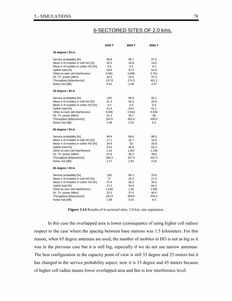
5.- SIMULATIONS 78
6-SECTORED SITES OF 2.0 kms.
2000 T 4000 T 6000 T
33 degree / 25 m
Service probability [%] 99.8 99.7 97.5Mean # of mobiles in soft HO [%] 20.5 19.8 19.5Mean # of mobiles in softer HO [%] 4.8 4.6 4.5Uplink load [%] 18.8 37.4 54.8Other-to-own cell interference 0.681 0.696 0.701DL TX. power [dBm] 30.4 34.5 37.6Throughput [kbps/sector] 137.8 274.3 401.1Noise rise [dB] 0.91 2.08 3.57
33 degree / 45 m
Service probability [%] 100 99.9 95.1Mean # of mobiles in soft HO [%] 31.4 30.2 29.9Mean # of mobiles in softer HO [%] 3.4 3.3 3.3Uplink load [%] 21.9 43.5 61.1Other-to-own cell interference 0.936 0.944 0.933DL TX. power [dBm] 31.3 35.7 39Throughput [kbps/sector] 152.5 302.6 430.5Noise rise [dB] 1.08 2.52 4.2
65 degree / 25 m
Service probability [%] 99.9 99.6 88.3Mean # of mobiles in soft HO [%] 17.1 16.7 16.6Mean # of mobiles in softer HO [%] 34.9 33 33.8Uplink load [%] 23.4 46.8 62.2Other-to-own cell interference 1.24 1.267 1.236DL TX. power [dBm] 31.6 36.3 39.5Throughput [kbps/sector] 166.3 327.4 437.4Noise rise [dB] 1.17 2.81 4.32
65 degree / 45 m
Service probability [%] 100 99.1 79.6Mean # of mobiles in soft HO [%] 27 26.3 27.4Mean # of mobiles in softer HO [%] 37.9 36.2 39.5Uplink load [%] 27.2 53.9 64.2Other-to-own cell interference 1.633 1.65 1.592DL TX. power [dBm] 32.5 37.6 40.5Throughput [kbps/sector] 183.9 359.6 444.2Noise rise [dB] 1.38 3.41 4.5
Figure 5.14 Results of 6-sectored sites, 2.0 km. site separation.
In this case the overlapped area is lower (consequence of using higher cell radius)
respect to the case where the spacing between base stations was 1.5 kilometers. For this
reason, when 65 degree antennas are used, the number of mobiles in HO is not as big as it
was in the previous case but it is still big, especially if we do not use narrow antennas.
The best configuration in the capacity point of view is still 33 degree and 25 meters but it
has changed in the service probability aspect: now it is 33 degree and 45 meters because
of higher cell radius means lower overlapped area and this is low interference level.

5.- SIMULATIONS 79
Figure 5.15 shows sector throughput as a function of DL traffic power for
different antenna configurations.
130
180
230
280
330
380
430
480
530
30 32 34 36 38 40 42
DL. AVERAGE TRAFFIC POWER [dBm]
SEC
TOR
TH
RO
UG
HPU
T [K
bps/
sect
or]
33_25
33_45
65_25
65_45
Figure 5.15 Sector throughput vs downlink traffic power with 6-sectored sites, 2.0 km. site separation.
In Figure 5.15 is again clearly displayed the saturation area of the network, but in
this case when the transmitted power exceeds 40.2 dBm. Nevertheless, when the best
configurations (33_25 and 33_45) are used, sector throughput grows with the transmitted
power even if the network is very high loaded. From the service probability point of
view, both configurations are the best when the network is loaded, especially the last one,
as shown in Figure 5.16, where is depicted the service probability as a function of sector
throughput.
75
80
85
90
95
100
130 180 230 280 330 380 430 480
SECTOR THROUGHPUT [Kbps/sector]
SER
VIC
E PR
OB
AB
ILIT
Y [%
]
33_2533_4565_2565_45
Figure 5.16 Service probability vs sector throughput with 6-sectored sites, 2.0 km. site separation.

5.- SIMULATIONS 80
6-SECTORED SITES OF 2.5 kms.
2000 T 4000 T 6000 T
33 degree / 25 m
Service probability [%] 99.5 99.2 96.3Mean # of mobiles in soft HO [%] 18.9 17.2 17.2Mean # of mobiles in softer HO [%] 4.9 4.7 4.6Uplink load [%] 18.1 36.1 52.7Other-to-own cell interference 0.656 0.673 0.677DL TX. power [dBm] 30 34 37Throughput [kbps/sector] 133.5 265.2 385.9Noise rise [dB] 0.88 2 3.4
33 degree / 45 m
Service probability [%] 100 99.9 96.1Mean # of mobiles in soft HO [%] 24.8 23.9 23.8Mean # of mobiles in softer HO [%] 3.8 3.7 3.7Uplink load [%] 20.2 40.3 58Other-to-own cell interference 0.824 0.837 0.835DL TX. power [dBm] 30.7 34.9 38.1Throughput [kbps/sector] 142.6 283.6 408.9Noise rise [dB] 0.99 2.29 3.88
65 degree / 25 m
Service probability [%] 99.5 98.5 85.4Mean # of mobiles in soft HO [%] 16.4 16.1 16.8Mean # of mobiles in softer HO [%] 32 30.3 31.9Uplink load [%] 23 46 60Other-to-own cell interference 1.243 1.276 1.247DL TX. power [dBm] 31.3 36 39.1Throughput [kbps/sector] 161.6 316.4 418Noise rise [dB] 1.15 2.77 4.11
65 degree / 45 m
Service probability [%] 100 98.7 81.9Mean # of mobiles in soft HO [%] 21.4 20.9 21.9Mean # of mobiles in softer HO [%] 35 33.5 35.8Uplink load [%] 25.5 50.7 62.8Other-to-own cell interference 1.474 1.499 1.456DL TX. power [dBm] 32 37 40Throughput [kbps/sector] 172.2 336.8 427.3Noise rise [dB] 1.29 3.15 4.38
Figure 5.17 Results of 6-sectored sites, 2.5 km. site separation.
Using maximum spacing between base stations, a reduction of the number of
mobiles in HO (increasing the cell radius decreases the overlapped area) is displayed in
the results. But when widebeam antennas are used, (65 degree) this number of mobiles in
HO is still more than two times bigger with respect to the case where narrowbeam
antennas (33 degree) have been used. In the capacity point of view, the best configuration
is still 33 degree and 25 meters, according to the results shown in Figure 5.17. In the
service probability aspect it is another time 33 degree and 45 meters (like when 2.0

5.- SIMULATIONS 81
kilometers site separation were used), but now the difference compared to the use of 25
meters antenna positions and 33 degree antenna beamwidth is bigger, respect to that case
of 2.0 kilometers site separation.
Figure 5.18 shows sector throughput as a function of DL traffic power for
different antenna configurations.
130
180
230
280
330
380
430
480
530
30 32 34 36 38 40 42
DL. AVERAGE TRAFFIC POWER [dBm]
SEC
TOR
TH
RO
UG
HPU
T [K
bps/
sect
or]
33_25
33_45
65_25
65_45
Figure 5.18 Sector throughput vs downlink traffic power with 6-sectored sites, 2.5 km. site separation.
In this case a peculiar event is depicted in Figure 5.18 because the best
configuration, 33_25, which is still giving the best results in capacity aspect, seems to be
saturated when the network load level is high. From the service probability point of view,
33_45 is the best configuration for any state of the network, as shown in Figure 5.19,
where is depicted the service probability as a function of sector throughput.
75
80
85
90
95
100
130 180 230 280 330 380 430 480
SECTOR THROUGHPUT [Kbps/sector]
SER
VIC
E PR
OB
AB
ILIT
Y [%
]
33_2533_4565_2565_45
Figure 5.19 Service probability vs sector throughput with 6-sectored sites, 2.5 km. site separation.

5.- SIMULATIONS 82
5.2.3.- Optimum Configurations
Results for the best configuration in 3-sector case are depicted in Figure 5.20. It is
65 degree antenna beamwidth and 25 meters of antenna height. The poorest results are
obtained with 1.5 kilometers between sites because the interference level is higher due to
they are too close to each other. When the site separation is bigger, there is a little fall in
the number of mobiles in HO, because of the smaller overlapped area. For those cases
where the site separation is higher than 1.5 kilometers, capacity level is always better,
particularly for 2.0 kilometers case, which is the best in this aspect, especially when the
network is loaded, because its saturation area begins later. For this load level, it gives
almost 4% more of capacity respect to the case of 2.5 kms (the second one in this aspect).
3-sectored sites with 65 degree antennas and base station antenna height of 25 m.
2000 T 3000 T 4000 T 5000 T 5500T
1.5 kilometers between BTS
Service probability [%] 100 98.7 86.1 70.4Mean # of mobiles in soft HO [%] 18.9 18.5 19.1 19.6Mean # of mobiles in softer HO [%] 4.8 4.7 5 5.3Uplink load [%] 38.6 57.3 66.4 67.9Other-to-own cell interference 0.744 0.751 0.729 0.707DL TX. power [dBm] 34.6 37.8 39.7 40.5Throughput [kbps/sector] 271.9 401.4 470.5 484.1Noise rise [dB] 2.14 3.77 4.81 4.98
2.0 kilometers between BTS
Service probability [%] 99.6 98.5 87.8 74.7 68.7Mean # of mobiles in soft HO [%] 16.5 16 16.2 16.2 16.1Mean # of mobiles in softer HO [%] 5.1 5 5.2 5.4 5.5Uplink load [%] 36.3 53.9 63.8 67 67.5Other-to-own cell interference 0.645 0.658 0.63 0.601 0.588DL TX. power [dBm] 34.3 37.4 39.2 40 40.3Throughput [kbps/sector] 266.7 394 469.6 499.6 503.4Noise rise [dB] 2 3.47 4.52 4.9 4.95
2.5 kilometers between BTS
Service probability [%] 99.1 97.1 86.1 64.9Mean # of mobiles in soft HO [%] 17.1 16.8 17.5 18.1Mean # of mobiles in softer HO [%] 5 5 5.3 5.7Uplink load [%] 35.9 53.2 62.8 65Other-to-own cell interference 0.672 0.684 0.656 0.61DL TX. power [dBm] 34.2 37.2 39.2 40.3Throughput [kbps/sector] 265.7 390 464.7 486.2Noise rise [dB] 1.98 3.41 4.43 4.66
Figure 5.20 Results of 3-sectored sites with 65 degree antennas and base station antenna height of 25 m.

5.- SIMULATIONS 83
Figure 5.21 shows sector throughput as a function of DL traffic power for
different site separation used.
250
300
350
400
450
500
550
34 35 36 37 38 39 40 41 42
DL. AVERAGE TRAFFIC POWER [dBm]
SEC
TOR
TH
RO
UG
HPU
T [K
bps/
sect
or]
1.5 kms
2.0 kms
2.5 kms
Figure 5.21 Sector throughput vs downlink traffic power for the best configuration with 3-sectored sites.
In Figure 5.22 is depicted the service probability as a function of sector
throughput. Also in this aspect, best results are obtained using 2.0 kilometers between
sites but now the worst case is not with a spacing of 1.5 kilometers.
65
70
75
80
85
90
95
100
250 300 350 400 450 500
SECTOR THROUGHPUT [Kbps/sector]
SER
VIC
E PR
OB
AB
ILIT
Y [%
]
1.5 kms2.0 kms2.5 kms
Figure 5.22 Service probability vs sector throughput for the best configuration with 3-sectored sites.
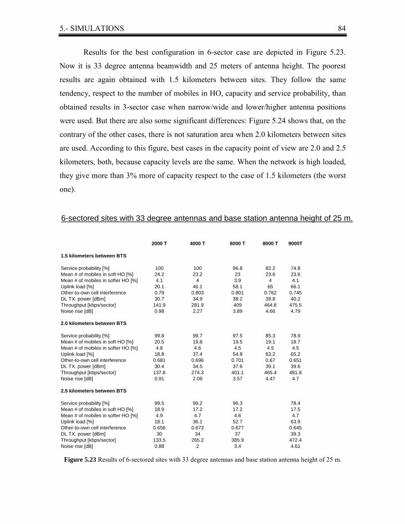
5.- SIMULATIONS 84
Results for the best configuration in 6-sector case are depicted in Figure 5.23.
Now it is 33 degree antenna beamwidth and 25 meters of antenna height. The poorest
results are again obtained with 1.5 kilometers between sites. They follow the same
tendency, respect to the number of mobiles in HO, capacity and service probability, than
obtained results in 3-sector case when narrow/wide and lower/higher antenna positions
were used. But there are also some significant differences: Figure 5.24 shows that, on the
contrary of the other cases, there is not saturation area when 2.0 kilometers between sites
are used. According to this figure, best cases in the capacity point of view are 2.0 and 2.5
kilometers, both, because capacity levels are the same. When the network is high loaded,
they give more than 3% more of capacity respect to the case of 1.5 kilometers (the worst
one).
6-sectored sites with 33 degree antennas and base station antenna height of 25 m.
2000 T 4000 T 6000 T 8000 T 9000T
1.5 kilometers between BTS
Service probability [%] 100 100 96.8 82.2 74.8Mean # of mobiles in soft HO [%] 24.2 23.2 23 23.6 23.6Mean # of mobiles in softer HO [%] 4.1 4 3.9 4 4.1Uplink load [%] 20.1 40.1 58.1 65 66.1Other-to-own cell interference 0.79 0.803 0.801 0.762 0.745DL TX. power [dBm] 30.7 34.9 38.2 39.8 40.2Throughput [kbps/sector] 141.9 281.9 409 464.8 475.5Noise rise [dB] 0.98 2.27 3.89 4.66 4.79
2.0 kilometers between BTS
Service probability [%] 99.8 99.7 97.5 85.3 78.9Mean # of mobiles in soft HO [%] 20.5 19.8 19.5 19.1 18.7Mean # of mobiles in softer HO [%] 4.8 4.6 4.5 4.5 4.5Uplink load [%] 18.8 37.4 54.8 63.2 65.2Other-to-own cell interference 0.681 0.696 0.701 0.67 0.651DL TX. power [dBm] 30.4 34.5 37.6 39.1 39.6Throughput [kbps/sector] 137.8 274.3 401.1 465.4 481.8Noise rise [dB] 0.91 2.08 3.57 4.47 4.7
2.5 kilometers between BTS
Service probability [%] 99.5 99.2 96.3 78.4Mean # of mobiles in soft HO [%] 18.9 17.2 17.2 17.5Mean # of mobiles in softer HO [%] 4.9 4.7 4.6 4.7Uplink load [%] 18.1 36.1 52.7 63.9Other-to-own cell interference 0.656 0.673 0.677 0.645DL TX. power [dBm] 30 34 37 39.3Throughput [kbps/sector] 133.5 265.2 385.9 472.4Noise rise [dB] 0.88 2 3.4 4.61
Figure 5.23 Results of 6-sectored sites with 33 degree antennas and base station antenna height of 25 m.

5.- SIMULATIONS 85
Figure 5.24 shows sector throughput as a function of DL traffic power for
different site separation used.
130
180
230
280
330
380
430
480
530
30 32 34 36 38 40
DL. AVERAGE TRAFFIC POWER [dBm]
SEC
TOR
TH
RO
UG
HPU
T [K
bps/
sect
or]
1.5 kms
2.0 kms
2.5 kms
Figure 5.24 Sector throughput vs downlink traffic power for the best configuration with 6-sectored sites.
Service probability as a function of sector throughput is depicted in Figure 5.25.
Also from this point of view, best results are obtained using 2.0 kilometers between sites.
In this aspect, the worst case is again the same: using a site separation of 2.5 kilometers.
75
80
85
90
95
100
130 180 230 280 330 380 430 480
SECTOR THROUGHPUT [Kbps/sector]
SER
VIC
E PR
OB
AB
ILIT
Y [%
]
1.5 kms
2.0 kms
2.5 kms
Figure 5.25 Service probability vs sector throughput for the best configuration with 6-sectored sites.

6.- CONCLUSIONS 86
6.- CONCLUSIONS
Coverage and capacity planning of UMTS WCDMA cellular networks cannot be
separated, since they are connected to each other. Furthermore, uplink and downlink
directions should be considered separately due to different (asymmetric) traffic.
Topology planning phase contains definition of key parameters like base station
antenna configuration (antenna beamwidth, antenna height or tilting), number of sectors
used in the sectoring process or description of base station locations: distance between
sites, etc. These elements have great impact on the system performance and they
influence strongly on capacity and service coverage of UMTS networks. All these
parameters should be defined in order to provide good coverage and capacity levels,
fulfiling QoSrequirements with reasonable implementation costs.
UMTS network capacity is interference limited, i.e. it is a soft capacity limited
system, because the interference rise in a cell causes the blocked calls. Interference level
is displayed in the simulation results, in section 5.2, and it decreases when the overlapped
area is smaller. If tilting is not considered (it has not been used in this work), the
capacity is higher when narrow antenna beamwidth and lower antenna positions are used.
Use of high antennas is better supported for the network when the distance between base
stations and/or the number of sectors/site are increased. Thus, when spacing between sites
is 2.5 kilometers, service probability is always better using narrow antennas with higher
antenna positions. This is due to higher antenna positions give larger coverage areas but
also higher interference level to neighbouring cells; nevertheless, when large spacing
between sites is used, the effect of better coverage has greater importance than
interference level. Antenna height affects the signal propagation near the base station and
antenna beamwidth allows to control softer HO areas, i.e. number of softer HOs, which
are needed in UMTS network in order to limit the interference level during the HO
procedure but should be taken into account that too large softer HO areas consumes
limited resources of the base station. Importance of a good choice for the base station
antenna beamwidth grows with the order of sectorisation.
In the aspect of spacing between sites, best results are obtained by using 2.0
kilometers between them, which is a middle value between 1.5 kms (better coverage but
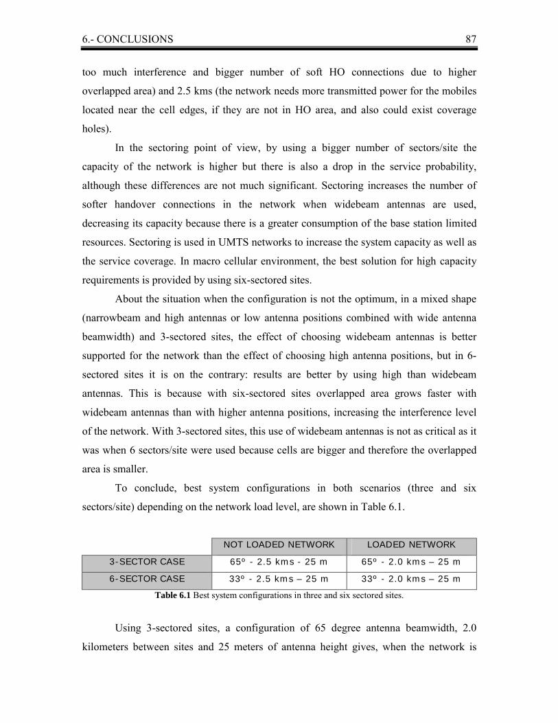
6.- CONCLUSIONS 87
too much interference and bigger number of soft HO connections due to higher
overlapped area) and 2.5 kms (the network needs more transmitted power for the mobiles
located near the cell edges, if they are not in HO area, and also could exist coverage
holes).
In the sectoring point of view, by using a bigger number of sectors/site the
capacity of the network is higher but there is also a drop in the service probability,
although these differences are not much significant. Sectoring increases the number of
softer handover connections in the network when widebeam antennas are used,
decreasing its capacity because there is a greater consumption of the base station limited
resources. Sectoring is used in UMTS networks to increase the system capacity as well as
the service coverage. In macro cellular environment, the best solution for high capacity
requirements is provided by using six-sectored sites.
About the situation when the configuration is not the optimum, in a mixed shape
(narrowbeam and high antennas or low antenna positions combined with wide antenna
beamwidth) and 3-sectored sites, the effect of choosing widebeam antennas is better
supported for the network than the effect of choosing high antenna positions, but in 6-
sectored sites it is on the contrary: results are better by using high than widebeam
antennas. This is because with six-sectored sites overlapped area grows faster with
widebeam antennas than with higher antenna positions, increasing the interference level
of the network. With 3-sectored sites, this use of widebeam antennas is not as critical as it
was when 6 sectors/site were used because cells are bigger and therefore the overlapped
area is smaller.
To conclude, best system configurations in both scenarios (three and six
sectors/site) depending on the network load level, are shown in Table 6.1.
NOT LOADED NETWORK LOADED NETWORK
3-SECTOR CASE 65º - 2.5 kms - 25 m 65º - 2.0 kms – 25 m
6-SECTOR CASE 33º - 2.5 kms – 25 m 33º - 2.0 kms – 25 m
Table 6.1 Best system configurations in three and six sectored sites.
Using 3-sectored sites, a configuration of 65 degree antenna beamwidth, 2.0
kilometers between sites and 25 meters of antenna height gives, when the network is

6.- CONCLUSIONS 88
loaded, a minimum of 17.2 Kbps/sector more of capacity (see Figure 5.20). If
throughput/user is 15 Kbps/user, this configuration allows, with the same QoS level, 65
users more in the network respect to other configurations.
Similarly, if 6-sectored sites are used, repeating the same analysis when the
network is loaded, this situation appears again, but now with 33 degree antennas, 2.0
kilometers between sites and 25 meters of antenna height. That configuration gives a
minimum of 9.4 Kbps/sector more of capacity (see Figure 5.23), which is equivalent to
71 users more in the network compared to other configurations.
In my opinion, in this point it is necessary to study the impact of tilting on
coverage and capacity of WCDMA systems because it has not been used in this work.
Maybe it can change the tendency shown by the results of this thesis, which indicate as
the best configuration for the base station antennas (when tilting is not used) narrowbeam
antennas and low antenna positions.

7.- REFERENCES 89
7.- REFERENCES
[1] Huang C., �An analysis of CDMA 3G wireless communications standards�, IEEE
Transactions on Vehicular Technology Conference, Vol.1, 1999, pp. 342-345.
[2] Chaudhury P., Mohr W. and Onoe S., �The 3GPP proposal for IMT-2000�, IEEE
Communications Magazine, Vol. 37, No. 12, December 1999, pp. 72-81.
[3] 3GPP web site, http://www.3gpp.org/.
[4] ETSI web site, http://www.etsi.org/.
[5] ITU web site, http://www.itu.int/imt/.
[6] UMTS forum web site, http://www.umts-forum.org/.
[7] 3GPP Technical Specification 23.907, �QoS concept�.
[8] Radio communications group of UPC web site, http://www.gcr.tsc.upc.es/.
[9] Ojanperä T. and Prasad R., �Overview of air interface multiple access for IMT-
2000/UMTS�, IEEE Communications Magazine, September 1998.
[10] Ojanperä T. and Prasad R., �Overview of air interface multiple access for IMT-
2000/UMTS�, IEEE Communications Magazine, September 1998, pp. 82-95.
[11] Prasad R., �CDMA for wireless personal communications�, Artech House, 1996.
[12] Redl S. M., Weber M. K. and Oliphant M. W., �An introduction to GSM�, Artech
House, 1995.

7.- REFERENCES 90
[13] IEEE web site, http://www.ieee.org/.
[14] Tanenbaum A. S., �Computer networks�, 3rd edition, Prentice-Hall, 1996.
[15] Cooper, G. R.. and McGillem, C. D., �Modern communications and spread
spectrum�, New York: Mc Graw-Hill Book Company, 1986.
[16] Lee J. S. and Miller L. E., �CDMA systems engineering handbook�, Artech
House, 1998.
[17] Peterson R. L., Ziemer R. E. and Borth D. E., �Introduction to spread spectrum
communications�, Prentice-Hall, 1995.
[18] Viterbi A. J., �CDMA: principles of spread spectrum communications�, Addison-
Wesley, 1995.
[19] 3GPP Technical Specification 25.213, �Spreading and modulation FDD�.
[20] Turkmani A. M. D. and Goni U. S., �Performance evaluation of maximal-length,
Gold and Kasami codes as spreading sequences in CDMA systems�, 2nd
International Conference on Universal Personal Communications, 1993, Vol. 2,
pp. 970-974.
[21] Dinan E. H. and Jabbari B., �Spreading codes for direct sequence CDMA and
Wideband CDMA cellular networks�, IEEE Communications Magazine,
September 1998, Vol. 3, No. 9, pp. 48-54.
[22] ARIB, �Japan´s proposal for candidate radio transmission technology on IMT-
2000: W-CDMA�, June 1998.

7.- REFERENCES 91
[23] Goel, G. and Pasrija, G., �3G CDMA proposals for mobile radio networks�,
Netaji Subhas Institute of Technology, Delhi University.
[24] Heiska, K., �Characteristics of the radiowave propagation in WCDMA�, Nokia
Networks, July 2002.
[25] 3GPP Technical Report 25.943, Deployment Aspects.
[26] Lempiäinen J. and Manninen M., �Radio interface system planning for
GSM/GPRS/UMTS�, Kluwer Academic Publishers, 2001.
[27] Ojanperä T. and Prasad R., �Wideband CDMA for third generation mobile
communications�, Artech House, 1998.
[28] Laiho, J. and Wacker, A., �Radio network planning process and methods for
WCDMA�, Annals of Telecommunications, Vol. 56, No. 5-6, May/June 2001, pp.
317-331.
[29] Holma H. and Toskala A., �WCDMA for UMTS�, John Wiley & Sons Ltd. 2000.
[30] Sipilä, K., Laiho-Steffens, J., Jäsberg, M. and Wacker, A., �Modelling the impact
of the fast power control on the WCDMA uplink�, Vehicular Technology
Conference, Houston, Texas, May 1999.
[31] Sipilä, K., Laiho-Steffens, J., Jäsberg, M. and Wacker, A., �Soft handover gains
in fast power controlled WCDMA uplink�, Vehicular Technology Conference,
Houston, Texas, May 1999.
[32] Coinchon M., Salovaara A. P. and Wagen J. F., �The impact of radio propagation
predictions on urban UMTS planning�, Broadband Communications, 2002.
Access, Transmission, Networking, pp. 32-1 to 32-6.

7.- REFERENCES 92
[33] Wacker A., Laiho J., Sipilä K. and Jäsberg M., �Static simulator for studying
WCDMA radio network planning issues�, Proceedings of IEEE Vehicular
Technology Conference, VTC1999, Houston, Texas, May 1999, pp. 2436-2440.
[34] Laiho J., Wacker A., Sipilä K. and Heiska K., �The impact of the subscriber
profile on WCDMA radio network performance�, Proceedings of IEEE Vehicular
Technology Conference, VTC1999, Houston, Texas, May 1999, pp. 2490-2494.
[35] Laiho-Steffens J., Wacker A., Sipilä K. and Heiska K., �The impact of the base
station sectorisation on WCDMA radio network performance�, Proceedings of
IEEE Vehicular Technology Conference, VTC1999, pp. 2611-2615.
[36] Niemelä J. and Lempiäinen J., �Impact of the base station antenna beamwidth on
capacity in WCDMA cellular networks�, Proceedings of IEEE Vehicular
Technology Conference, VTC2003.
[37] Laiho-Steffens J., Wacker A. and Aikio P., �The impact of the radio network
planning and site configuration on the WCDMA network capacity and quality of
service�, Proceedings of IEEE Vehicular Technology Conference, VTC2000, pp.
1006-1010.
[38] Christer B., Johansson V. and Stefansson S., �Optimizing antenna parameters for
sectorized W-CDMA networks�, Proceedings of IEEE Vehicular Technology
Conference, VTC2000, pp. 1524-1531.
[39] Forkel I., Kemper A., Pabst R. and Hermans R., �The effect of electrical and
mechanical antenna down-tilting in UMTS networks�, Proceedings of 3G 2002,
Third International Conference on 3G Mobile Communication Technologies,
London, UK, May 2002, pp. 86-90.

7.- REFERENCES 93
[40] Laiho J., Wacker A. and Novosad T., �Radio network planning and optimization
for UMTS�, John Wiley & Sons Ltd, 2002.
[41] UMTS Forum Report 5, �Minimum spectrum demand per public terrestrial
UMTS operator in the initial phase�, September 1998.
[42] UMTS Forum Report 6, �UMTS/IMT-2000 spectrum�, December 1998.
[43] Ganz A., Krishna C. M., Tang D. and Haas Z. J., �An optimal design of multitier
wireless cellular systems�, IEEE Communications Magazine, Vol. 35, No. 2,
February 1997, pp. 88-93.
APPENDIX 94
APPENDIX List of Acronyms
AC Admission Control
ARIB Association of Radio Industries and Businesses
BCCH Broadcast Control Channel
BER Bit Error Rate
BPSK Binary PSK
BS BTS
BTS Base Station
CCPCH Common Control Physical Channel
CDMA Code Division Multiple Access
CIR Carrier to Interference Ratio
CN Core Network
DAS Distributed Antenna Systems
DL Downlink
DPCCH Dedicated Physical Control Channel
DPDCH Dedicated Physical Data Channel
DS Direct Sequence
DTX Discontinuous Transmission
Eb/N0 Bit Energy to Noise Ratio
EIRP Equivalent Isotropic Radiated Power
EMC Electromagnetic Compatibility
ETSI European Telecommunications Standards Institute
FACH Forward Access Channel
FDD Frequency Domain Duplex
FDMA Frequency Division Multiple Access
FFT Fast Fourier Transformation
FH Frequency Hopping

APPENDIX 95
GGSN Gateway GPRS Support Node
GMSC Gateway MSC
GPRS General Packet Radio Service
GSM Global System Mobile
HC Handover Control
HCS Hierarchical Cell Structure
HLR Home Location Register
HM Hybrid Modulation
HO Handover / Handoff
IEEE Institute of Electrical and Electronics Engineers
IMT International Mobile Telephony
IQ In-Phase Quadrature
ISI Intersymbol Interference
IT Information Technologies
ITU International Telecommunication Union
LAN Local Area Network
LC Load Control
LNA Low Noise Amplifier
LOS Line of Sight
LPI Low Probability of Intercept
MC Multicarrier
ME Mobile Equipment
MS Mobile Station
MSC Mobile Services Switching
MSK Minimum Shift Keying
MUD Multi User Detection
NB Narrowband
PC Power Control
PCH Paging Channel
PDF Probability Density Function
PDP Power Delay Profile

APPENDIX 96
PLMN Public Land Mobile Network
PN Pseudo-random Noise-like
PS Packet Scheduling
PSK Phase Shift Keying
QoS Quality of Service
QPSK Quadrature PSK
RNC Radio Network Controller
RNS Radio Network Subsystem
RRM Radio Resource Management
RTT Radio Transmission Technology
RX Receiver
SCH Synchronization Channel
SDU Service Data Unit
SGSN Serving GPRS Support Node
SHO Soft HO
SIR Signal to Interference Ratio
SMS Systems Management Server
SNR Signal to Noise Ratio
SS Spread Spectrum
TDD Time Domain Duplex
TDMA Time Division Multiple Access
TH Time Hopping
TPC Transmission Power Control
TX Transmitting
UE User Equipment
UL Uplink
UMTS Universal Mobile Telecommunications System
USIM UMTS Subscriber Identity Module
UTRAN UMTS Terrestrial Radio Access Network
VCoIP Video Conferencing over IP
VLR Visitor Location Register

APPENDIX 97
VoIP Voice over IP
WB Wideband
WCDMA Wideband CDMA
3GPP 3rd Generation Partnership Project

APPENDIX 98
List of Tables
1.1.- 2G vs 3G ��������������������������. pag. 8
2.1.- QoS classes in UMTS���������������������. pag. 12
2.2.- Typical powers for the downlink common channels���������.. pag. 19
3.1.- Main parameters WCDMA for UMTS��������������... pag. 36
3.2.- Path loss exponents according to the environment type��������. pag. 38
3.3.- Characteristics for different radio propagation environments������ pag. 40
4.1.- General information of the power budget calculation...��������.. pag. 47
4.2.- WCDMA power budget in simulations.............................�������.. pag. 51
4.3.- Okumura-Hata model parameters as a function of frequency..............��.. pag. 53
4.4.- Typical maximum allowed path loss of existing GSM and WCDMA
systems........................................................................................................... pag. 54
4.5.- K-values for the site area calculation............................��������.. pag. 54
4.6.- Simulation values of the network topology parameters��������.. pag. 61
4.7.- Ranges and applications of the different UMTS cell types......�����.. pag. 64
5.1.- Advantages and disadvantages of WCDMA simulation methods����.. pag. 66
5.2.- Total number of terminals in the network according to its load level��� pag. 69
6.1.- Best system configurations in three and six sectored sites�������.. pag. 87

APPENDIX 99
List of Figures
1.1.- Increase of mobile telephone and Internet users in the last 10 years��� pag. 8
2.1.- UMTS network architecture������������������. pag. 13
2.2.- Block diagram of the UTRAN and CN��...�����������. pag. 15
2.3.- Parallel transmission of DPDCH and DPDCCH channels when the data
is present/absent���...������������������� pag. 16
2.4.- Structure of WCDMA random access burst������������. pag. 17
2.5.- Packet transmission on a common channel������������.. pag. 20
3.1.- Multiple access schemes�������������������.. pag. 23
3.2.- Principle of spread spectrum technique..�������������. pag. 24
3.3.- Classification of CDMA types ����������������� pag. 25
3.4.- Despreading of a wideband signal in the presence of a narrowband
interferer�������������������������.. pag. 26
3.5.- Example of generation of the CDMA transmitted signal������� pag. 28
3.6.- 2nd example of generation of the CDMA transmitted signal�����. pag. 29
3.7.- Basic block diagram of a RAKE receiver in a L � tap channel����... pag. 32
3.8.- Frequency use with WCDMA�����������������. pag. 34
3.9.- Radio propagation environment classes�������������.. pag. 37
3.10.- Two ray-model in multi path propagation������������... pag. 39
3.11.- Channel impulse response of a typical urban channel �������� pag. 39
3.12.- Log-normal distribution�������������������.. pag. 41
3.13.- Rayleigh distribution��������������������... pag. 41
3.14.- Frequency response of Rayleigh channel ������������.. pag. 42
4.1.- WCDMA radio network planning process�..����������� pag. 45
4.2.- Interference degradation margin as a function of load������..�.. pag. 49
4.3.- Path loss as a function of distance by using Okumura-Hata model.��... pag. 53
4.4.- Mutual influence of coverage and capacity in WCDMA networks��.... pag. 55

APPENDIX 100
4.5.- Impact of coverage and capacity on WCDMA network design..���� pag. 56
4.6.- Cell structure for three and six sectors/site������������.. pag. 59
4.7.- Coverage vs interference level����������������� pag. 59
4.8.- A hierarchical cell scenario in UMTS��������������. pag. 62
5.1.- Digital map of the simulation area���������������� pag. 68
5.2.- Results of 3-sectored sites, 1.5 km. site separation���������... pag. 70
5.3.- Sector throughput vs downlink traffic power with 3-sectored sites,
1.5 km. site separation��������������������.. pag. 71
5.4.- Service probability vs sector throughput with 3-sectored sites, 1.5 km.
site separation�����������������������... pag. 71
5.5.- Results of 3-sectored sites, 2.0 km. site separation���������.. pag. 72
5.6.- Sector throughput vs downlink traffic power with 3-sectored sites,
2.0 km. site separation��������������������. pag. 73
5.7.- Service probability vs sector throughput with 3-sectored sites, 2.0 km.
site separation�����������������������.. pag. 73
5.8.- Results of 3-sectored sites, 2.5 km. site separation���������.. pag. 74
5.9.- Sector throughput vs downlink traffic power with 3-sectored sites,
2.5 km. site separation��������������������. pag. 75
5.10.- Service probability vs sector throughput with 3-sectored sites, 2.5 km.
site separation�����������������������... pag. 75
5.11.- Results of 6-sectored sites, 1.5 km. site separation���������.. pag. 76
5.12.- Sector throughput vs downlink traffic power with 6-sectored sites,
1.5 km. site separation��������������������.. pag. 77
5.13.- Service probability vs sector throughput with 6-sectored sites, 1.5 km.
site separation�����������������������... pag. 77
5.14.- Results of 6-sectored sites, 2.0 km. site separation���������.. pag. 78
5.15.- Sector throughput vs downlink traffic power with 6-sectored sites,
2.0 km. site separation��������������������. pag. 79
5.16.- Service probability vs sector throughput with 6-sectored sites, 2.0 km.
site separation�����������������������... pag. 79
APPENDIX 101
5.17.- Results of 6-sectored sites, 2.5 km. site separation���������.. pag. 80
5.18.- Sector throughput vs downlink traffic power with 6-sectored sites,
2.5 km. site separation��������������������.. pag. 81
5.19.- Service probability vs sector throughput with 6-sectored sites, 2.5 km.
site separation�����������������������... pag. 81
5.20.- Results of 3-sectored sites with 65 degree antennas and base station
antenna height of 25 m�������������������..... pag. 82
5.21.- Sector throughput vs downlink traffic power for the best configuration
with 3-sectored sites���������������������. pag. 83
5.22.- Service probability vs sector throughput for the best configuration with
3-sectored sites�����������������������. pag. 83
5.23.- Results of 6-sectored sites with 33 degree antennas and base station
antenna height of 25 m��������������������. pag. 84
5.24.- Sector throughput vs downlink traffic power for the best configuration
with 6-sectored sites���������������������. pag. 85
5.25.- Service probability vs sector throughput for the best configuration with
6-sectored sites�����������������������. pag. 85

APPENDIX 102
Simulation Parameters BS maximum power [dBm] 43
CPICH [dBm] 33
CCCHs [dBm] 33
SCH [dBm] 33
Maximum power per connection [dBm] 33
BS noise figure [dB] 5
UL required Eb/N0 [dB] 5
MS maximum power [dBm] 21
MS dynamic range [dB] 70
Power control step size [dB] 0.5
Required Ec/I0 [dB] -18
MS noise figure [dB] 9
DL required Eb/N0 [dB] 8
Standard deviation of slow fading [dB] 10
UL noise rise [dB] 6
DL orthogonality [%] 60
Handover window [dB] 4
Standard deviation of power control [dB] 0.5
Total number of carriers 1
Carrier frequency [MHz] 2000
UL air interface bit rate [Kbps] 15
UL user bit rate [Kbps] 15
DL air interface bit rate [Kbps] 15
DL user bit rate [Kbps] 15
Voice activity factor [%] 50

APPENDIX 103
UL Eb/N0 [dB] 5
DL Eb/N0 [dB] 8
Propagation model Okumura-Hata
Constant C 44.15
MS height [meters] 1.5
Average area type correction [dB] - 6.7
Standard deviation of interference [dB] 7.5
Simulation resolution [meters] 5
Chip rate [Mcps] 3.84
Intra-site correlation coefficient 0.8
Inter-site correlation coefficient 0.5
ANTENNAS kathrein 33: - 45 degree polarized, system lever position 0 degree
θ-3dB : vertical → 6.0 degree Gain [dBd] 18.85
horizontal → 31.0 degree

APPENDIX 104
kathrein 65: - 45 degree polarized, system lever position 0 degree
θ-3dB : vertical → 6.0 degree Gain [dBd] 15.85
horizontal → 61.5 degree
kathrein 90: - 45 degree polarized, system lever position 0 degree
θ-3dB : vertical → 6.0 degree Gain [dBd] 14.55
horizontal → 87.5 degree
Related Documents