Impact assessment of rainfall scenarios and land-use change on hydrologic response using synthetic Area IDF curves

Impact assessment of rainfall

scenarios and land-use change on

hydrologic response using synthetic

Area IDF curves

Pingping Luo1),2), Apip3), Bin He4), Weili Duan4),Kaoru Takara5),

Daniel Nover6)

1) State Key Laboratory of Lake Science and Environment

(SKLLSE), Nanjing Institute of Geography and Limnology, Chinese

Academy of Sciences (CAS), Nanjing, China

2) United Nations University - Institute for the Advanced Study

of Sustainability (UNU-IAS), Shibuya, Tokyo, Japan

E-mail: [email protected]

3) Research Centre for Limnology, Indonesian Institute of

Sciences (LIPI), Indonesia

4) State Key Laboratory of Lake Science and Environment

(SKLLSE), Nanjing Institute of Geography and Limnology, Chinese

1

1

2

3

4

5

6

7

8

9

10

11

12

13

14

15

16

17

18

Academy of Sciences (CAS), Nanjing, China

5) Disaster Prevention Research Institute (DPRI), Kyoto

University, Uji, Kyoto, Japan

6) AAAS Science and Technology Policy Fellow, U.S. Agency for

International Development, Ghana, West Africa

This paper has been modified in the final version. Please check

the published paper.

Please cite this paper by using the following citation:

Luo, P., Apip, He, B., Duan, W., Takara, K. and Nover, D.

(2015), Impact assessment of rainfall scenarios and land-use

change on hydrologic response using synthetic Area IDF curves.

Journal of Flood Risk Management. doi: 10.1111/jfr3.12164

Abstract

In combination with land use change, climate change is

increasingly leading to extreme weather conditions and

consequently novel hydrologic conditions. Rainfall Area

Intensity-Duration-Frequency (IDF) curves, commonly used tools

for modeling hydrology and managing flood risk, can be used to

assess hydrologic response under extreme rainfall conditions.

We explore the influence of land use change on hydrologic

2

19

20

21

22

23

24

25

26

27

28

29

30

31

32

33

34

35

36

37

38

39

response under designed extreme rainfall over the period 1976

to 2006 in the Kamo River basin. Runoff for all six designed

rainfall shapes under 2006 land use is higher than that under

1976 land use, but the timing of peak discharge under 2006 land

use occurs at roughly the same time as that under 1976 land

use. Results indicate that runoff under 2006 land use yielded

higher discharge than under 1976 land use, and shape 6 leads to

the most extreme hydrologic response and most dangerous

conditions from the perspective of urban planning and flood

risk management. Future hydrologic response will differ from

present due both to changes in land-cover and changes in

extreme rainfall patterns requiring modification to Area IDF

curves for catchments.

Keywords: scenario, land use change, Area IDF, extreme runoff,

hydrologic response, design storm

3

40

41

42

43

44

45

46

47

48

49

50

51

52

53

54

55

56

57

58

59

60

1. Introduction

Human activities and consequent land use change are dominant

factors contributing to changes in watershed hydrology.

Catchment hydrology is affected by changes in land cover, soil

type, geology, climate, and land use. Storm temporal dynamics

including duration and intensity are important drivers of

hydrologic response. Area Intensity-Duration-Frequency (IDF)

curves are a set of tools that summarize the relationship

between precipitation dynamics (intensity, duration and

frequency) that can be used to explore catchment hydrology.

Better flood risk management in urban catchments requires an

understanding both of the impact of rainfall shape and land use

change on hydrologic response and the way that Area IDF curves

must change as climate change alters our understanding of storm

intensity, duration and frequency.

Land use change can change flood frequency (Brath et al.,

2006; Crooks and Davies, 2001), flood severity (De Roo et al.,

2001), base flow (Wang et al., 2006), and annual mean discharge

4

61

62

63

64

65

66

67

68

69

70

71

72

73

74

75

76

77

78

79

80

81

(Costa et al., 2003). The impact of land use change on

hydrologic response as well as the link between land use and

evapotranspiration regimes has been studied with regard to

catchment hydrology (Dunn and Mackay, 1995). Wijesekara et al.

(2012) extended the land use change impacts assessment from

past to future period on hydrologic processes. However, the

previous land use change assessment studies have not examined

the impact of extreme rainfall timing and distribution on

hydrologic response. Statistical methods have been used to

assess the effect of urbanization and riparian vegetation on

watershed hydrology in Los Penasquitos Creek, California (White

and Greer, 2006). Reconstructed geomorphological evidence

combined with one-dimensional hydraulic modeling has also been

used to analyze the combined effect of late Holocene climatic

variability and land use change in the Guadalentín River,

southeast Spain (Benito et al., 2010). A simple daily rainfall-

runoff model was used to assess the impact of land use change

on catchment hydrology in the Comet River, Central Queensland,

Australia (Siriwardena et al., 2006). To study the long-term

land use change impact on the hydrological response, the new

technology of historical land use reconstruction called Paleo-

5

82

83

84

85

86

87

88

89

90

91

92

93

94

95

96

97

98

99

100

101

102

Land Use Reconstruction (PLUR) model has been developed by Luo

et al. (2014a). For the research on the paleo-hydrology, the

new research framework is introduced by using the modern

technology, hydrological model, statistic method, the PLUR

model and other method (Luo et al., 2014b). The long-term land

use change has been significantly affected at the flood risk.

Changing the land use such as from the farmland to lake area,

from urban area to forest area and so on could be considering

as a useful policy for the flood management purpose (Luo et

al., 2015). By combining the land use change impact assessment

with the reconstruction on paleo-hydrology, it will provide

more powerful evidence for the effect of human activities on

flood events.

Rainfall intensity can be expressed in volume units when

summed over time and space. Storm events can be expressed as

idealized ‘design storms’ in engineering hydrology and the

‘shapes’ of these design storms can be used to analyze

hydrologic response in a given catchment. Analysis of land use

change impact on hydrologic response can be achieved using a

suite of tools, including distributed hydrological models and

relationships expressed through IDF curves. Sub-interval

6

103

104

105

106

107

108

109

110

111

112

113

114

115

116

117

118

119

120

121

122

123

(months or years) selection and series of rainfall events

exceeding a given threshold were experimentally compared for

estimating rainfall IDF relations from fragmentary records

(Svensson, 2007). Nhat et al. (2007) found that IDFs had a

strong relationship with the area of the catchment and proposed

the use of Area-Intensity-Duration-Frequency (AIDF) curves. Two

different regimes for areas of 110 km2 and 992 km2 in the Yodo

River basin were calculated with hourly simple time.

Kyoto, which is bisected by the Katsura River and the Kamo

River experienced extreme rainfall during Typhoon No. 18 from

September 15-16, 2013. Water levels in the Katsura River and

the Uji River reached dangerous flood stages within 6 hours of

the beginning of the rainfall event and the Arashiyama area

near the Katsura River was flooded. Identifying rainfall

conditions that could lead to high and fast peak discharge is

extremely important, particularly as land use change is leading

to conditions that promote such hydrologic response. The basins

surrounding this part of Japan are therefore selected as a

study area to inform water resources managers as they attempt

to address shifting patterns of precipitation and land use

change.

7

124

125

126

127

128

129

130

131

132

133

134

135

136

137

138

139

140

141

142

143

144

The main purpose of this study is to investigate the

influence of land use change under designed rainfall from the

Area IDF curves with different return periods, duration and

shapes on urban catchment hydrologic response using the grid-

based distributed rainfall-runoff model version3 (CDRMV3). Six

design storms based on the Area IDF are selected at the Yodo

river basin. We present two additional historical storms based

on the Area IDF. It presents discharge under 1976 and 2006 land

use with 50, 100 and 200 years flood return period for the six

design storms. The results of this study have important

implications for understanding the relationship between

hydrology and land use change in addition to the hydrology of

flood events. A discussion has been given on incorporating

climate change into Area IDF curves and scenario simulation of

extreme runoff. This work is conducted with the ultimate goal

of supporting flood risk management under ever changing

management contexts.

2. Study site and data

2.1 Study site

There are six sub-basins in the Yodo River basin (YRB)

including the Lake Biwa basin (3,802 km2), the Uji River basin

8

145

146

147

148

149

150

151

152

153

154

155

156

157

158

159

160

161

162

163

164

165

(506 km2), the Kizu River basin (1,647 km2), the Katsura River

basin (1,152 km2), the lower Yodo River basin (521 km2) and the

Kanzaki River basin (612 km2). Kyoto Prefecture is situated in

the union of the Katsura River, Kizu River and Uji River where

the YRB connects to the lower Yodo River and flows to Osaka

Bay. Mountainous terrain comprises about 71.9% and flat area

comprises about 28.1% of the YRB. The mean annual precipitation

of the basins of Lake Biwa, the Katsura River, the Kizu River,

and the lower Yodo River basins are about 1,880, 1,640, 1,590,

and 1,400 mm respectively. Mean annual precipitation in the YRB

is 1387.8 mm (1976 ~ 2000) and mean annual runoff in the YRB is

270.8 m3/s (1952 ~1998) at Hirakata.

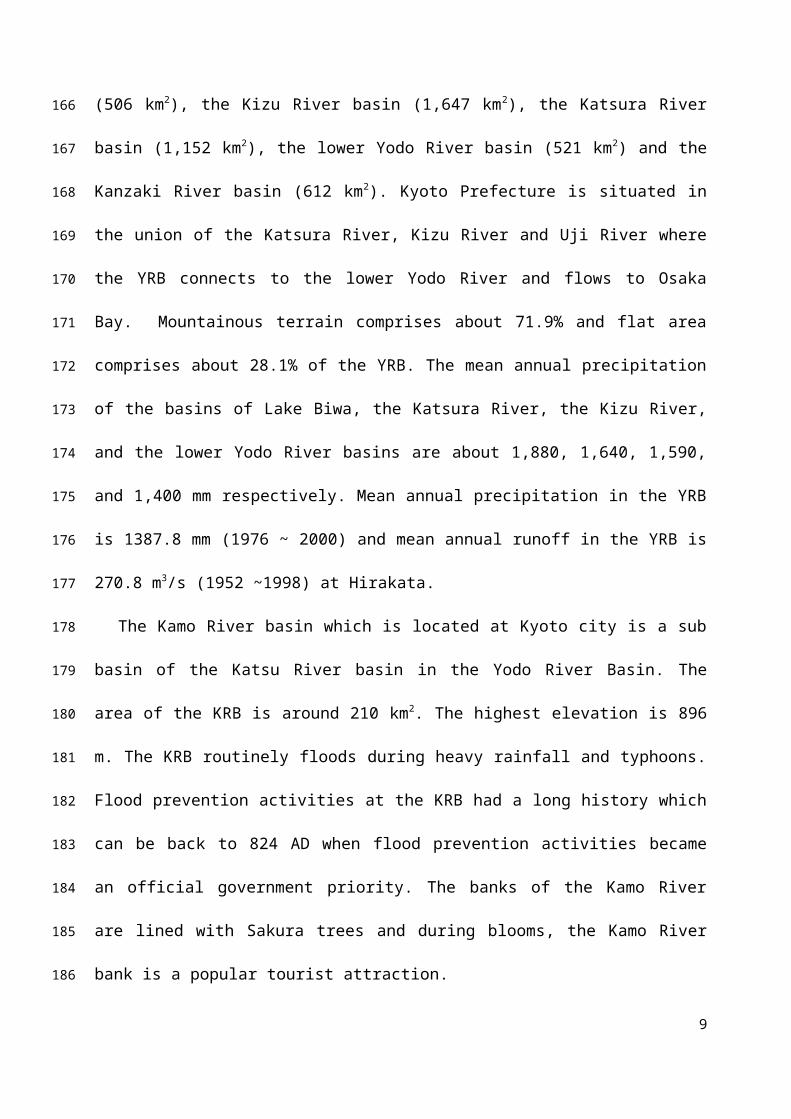
The Kamo River basin which is located at Kyoto city is a sub

basin of the Katsu River basin in the Yodo River Basin. The

area of the KRB is around 210 km2. The highest elevation is 896

m. The KRB routinely floods during heavy rainfall and typhoons.

Flood prevention activities at the KRB had a long history which

can be back to 824 AD when flood prevention activities became

an official government priority. The banks of the Kamo River

are lined with Sakura trees and during blooms, the Kamo River

bank is a popular tourist attraction.

9

166

167

168

169

170

171

172

173

174

175

176

177

178

179

180

181

182

183

184

185

186

2.2 Data

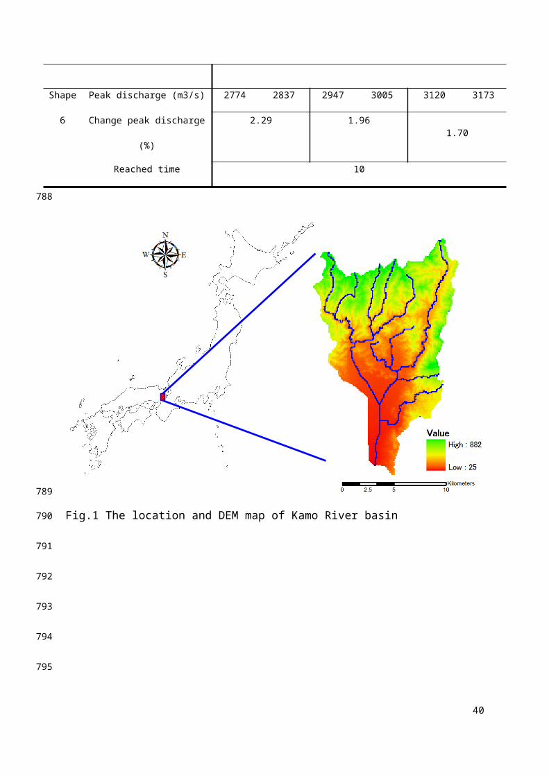
We collected spatial and hydrologic data from the Kamo River

basin including Digital Elevation Model (DEM), land use,

channel network, observed discharge and Automated

Meteorological Data Acquisition System (AMeDAS) data from the

Japan Ministry of Land, Infrastructure, Transport and Tourism

(MLIT). The 50-m resolution DEM data (Fig.1) and 100-m mesh

land use data sheets from 2006 (Fig.2) and 1976 (Fig.2) were

obtained from the National and Regional Planning Bureau of

MLIT. The DEM map in this study was scaled up from 50 to 100 m

by using ArcGIS 10. Table 1 shows the detail land use types in

1976 and 2006.

The observed discharge from September 25-26, 1953, at

Fukakusa is used for calibrating the CDRMV3 in the Kamo river

basin. Design storms of duration 10 and 20 hours with return

periods of 50, 100 and 200 years are made based on results from

Naht et al. (2007) using IDF curves for the Yodo River basin.

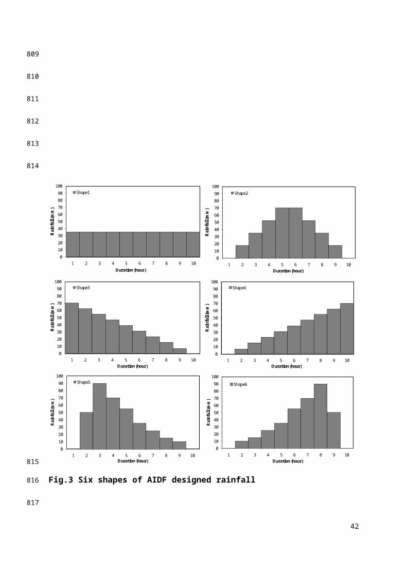
Fig. 3 shows the six design rainfall shapes used in this study.

The hourly rainfall of Shape 1 uses the average value for 10

hours rainfall. Shape 2 has peak rainfall in the middle hour.

Shape 3 has peak rainfall in the first hour. Shape 4 shows the

10

187

188

189

190

191

192

193

194

195

196

197

198

199

200

201

202

203

204

205

206

207

peak rainfall in the last hour. Shape 5 has peak rainfall in

the first few hours. Shape 6 has peak rainfall before the last

few hours.

3. Methods

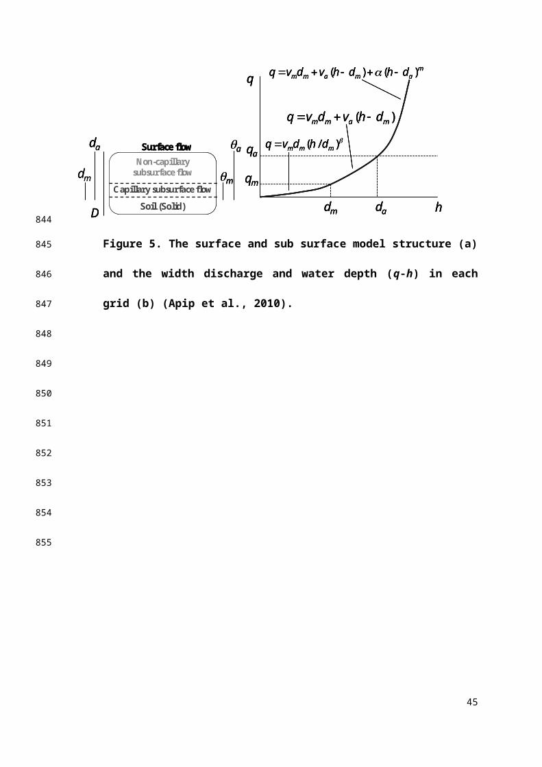
3.1 Grid-based hydrological model

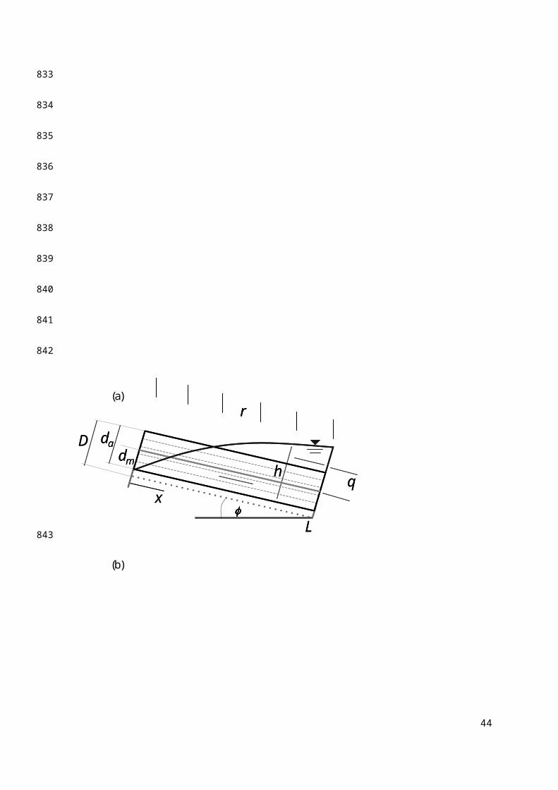
This study uses CDRMV3 model, which uses the Kinematic wave

equation combined with the Lax Wendroff scheme at every node of

each cell (Kojima, 1997) to calculate the surface and

subsurface hydrologic processes in each grid cell. CDRMV3

simulates the dominant lateral flow mechanisms including (1)

subsurface flow through capillary pores, (2) subsurface flow

through non-capillary pores and (3) surface flow on the soil

layer. Flow is simulated suing Darcy’s law with an unsaturated

hydraulic conductivity km at each grid-cell when the water depth

is below the equivalent water depth for unsaturated flow (0 h

dm). The model includes a stage-discharge, q-h relationship

for both surface and subsurface runoff processes (Fig.5) (Apip

et al., 2010; Luo et al., 2013):

q={ vm∗dm∗(hdm

)θ

0≤h≤dm

vm∗dm+va∗(h−dm) dm≤h≤davm∗dm+va∗(h−dm )+α∗(h−da)

m da≤h

(1)

11

208

209

210

211

212

213

214

215

216

217

218

219

220

221

222

223

224

225

226

vm=kmi,va=kai,km=kaθ,α=√i/n

dm=Dθm,da=Dθa

where q is the discharge per unit width, h (mm) is the water

depth, i is the slope gradient, km (mms-1) is the saturated

hydraulic conductivity of the capillary soil layer, ka (mms-1) is

the hydraulic conductivity of the non-capillary soil layer

(saturated), dm (mm) is the depth of the capillary soil layer

(unsaturated), da (mm) is the depth of the capillary and non-

capillary soil layer, vm and va are the flow velocities of

unsaturated and saturated subsurface flows respectively, θ is a

non-dimensional parameter for unsaturated flow, θa is the

effective porosity of the soil layer (D), θm is the effective

porosity of the unsaturated layer, and n (m-1/3s) is the

Manning's roughness coefficient based on the land cover

classes.

3.2 Monte Carlo approach

Monte Carlo approach (MCA) is the technique used in this

study for calibration and uncertainty analysis of the

hydrologic model. MCA is used here to statistically

characterize all model parameters by running hundreds or

12

227

228

229

230

231

232

233

234

235

236

237

238

239

240

241

242

243

244

245

246

thousands of iterations to generate multiple outputs, including

runoff flow for a catchment. MCA approximates stochastic

processes by generating a large number of equally probably

realizations of model parameters according to their

corresponding probability distributions with lower and upper

bounds that are assumed to represent the variation of

calibration parameters. MCA uses random numbers and probability

to solve problems, iteratively evaluating a deterministic model

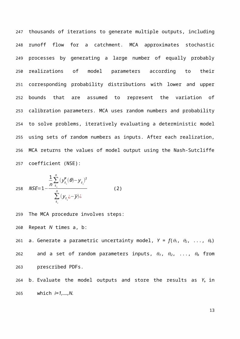
using sets of random numbers as inputs. After each realization,

MCA returns the values of model output using the Nash-Sutcliffe

coefficient (NSE):

NSE=1−

1n∑ti

n(yti

M (θ)−yti)2

∑ti

n(yti

¿−y)¿

(2)

The MCA procedure involves steps:

Repeat N times a, b:

a. Generate a parametric uncertainty model, Y = f(1, 2, ..., k)

and a set of random parameters inputs, i1, i2, ..., ik from

prescribed PDFs.

b. Evaluate the model outputs and store the results as Yi, in

which i=1,….,N.

13

247

248

249

250

251

252

253

254

255

256

257

258

259

260

261

262

263

264

265

The Monte Carlo method is just one of many methods for

analyzing uncertainty propagation and is widely used in

hydrologic models. However, the application of the method is

affected by the appropriateness of the chosen Probability

Distribution Functions (PDFs) for sampling random parameter

values and the number simulations used.

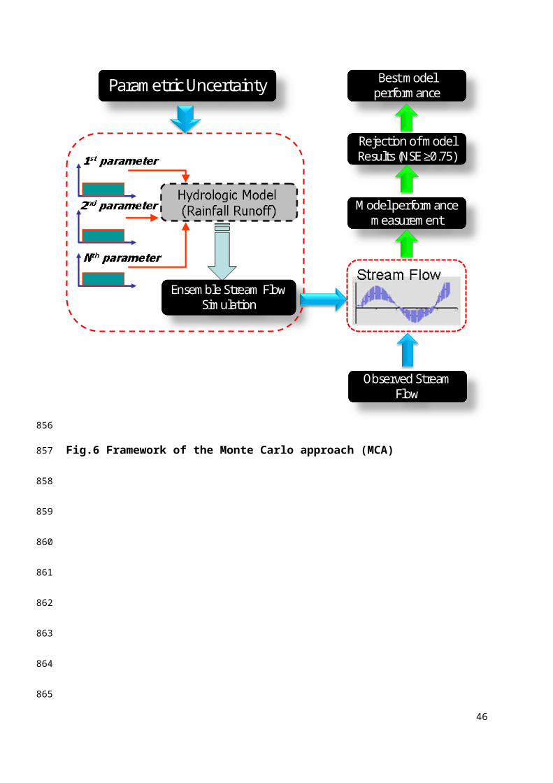
Detail explanation of the MCA process used in this study is

presented in Fig.6. For parametric uncertainty, a set of random

parameters inputs (1st parameter, 2nd parameter,…, Nth

parameter) is input to the hydrologic model to get ensemble

stream flow simulations. The observed stream flow is used to

measure the model performance. The objective function NSE is

used to evaluate the model simulation. If the coefficient of

model results (NSE) is over 0.75, this parameter set will

selected. The process is repeated again until the nth

simulation. Finally, the best model performance is chosen from

the selected parameter sets with NSE is over 0.75.

3.3 Area Intensity-Duration-Frequency (IDF)

All forms of the generalized IDF relationships assume that

rainfall depth or intensity is inversely related to the

duration of a storm raised to a power, or scale factor (Chow et

14

266

267

268

269

270

271

272

273

274

275

276

277

278

279

280

281

282

283

284

285

286

al., 1988). There are several researches found in the

literature for hydrologic applications (Chen, 1983; Hershfied,

1961; VanNguyen et al., 2002; Bell, 1969). Koutsoyiannis et al.

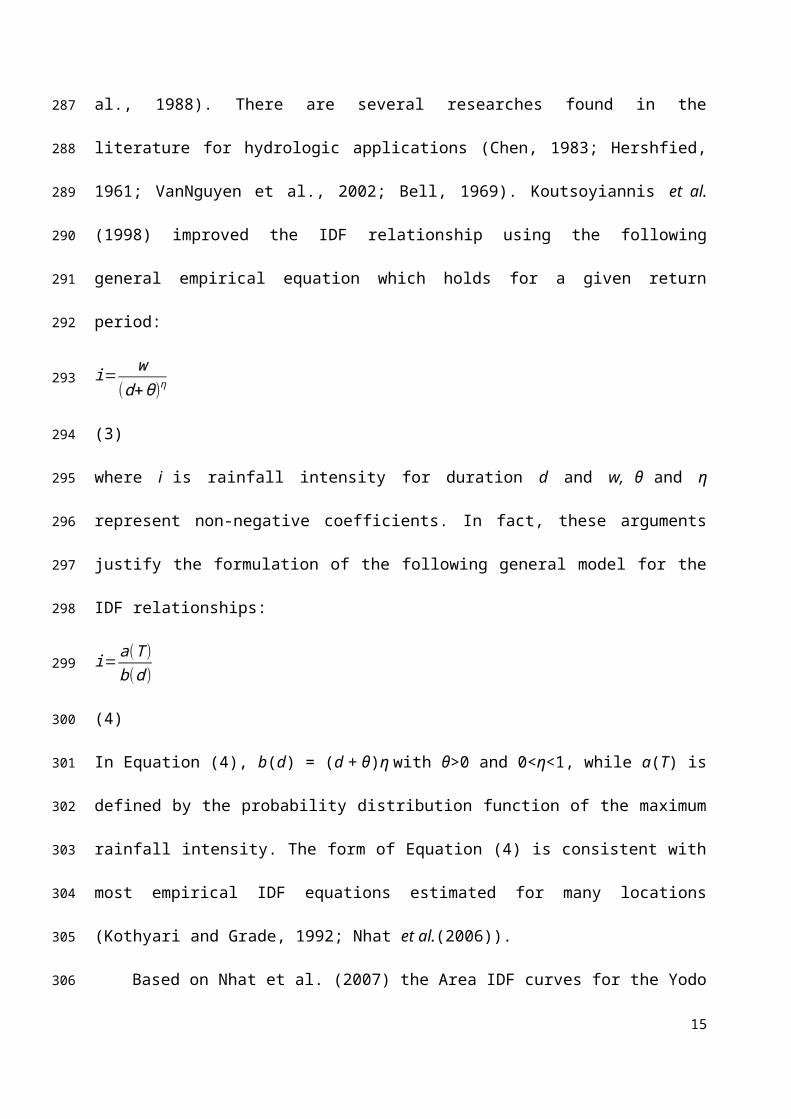
(1998) improved the IDF relationship using the following

general empirical equation which holds for a given return

period:

i= w(d+θ)η

(3)

where i is rainfall intensity for duration d and w, θ and η

represent non-negative coefficients. In fact, these arguments

justify the formulation of the following general model for the

IDF relationships:

i=a(T)b(d)

(4)

In Equation (4), b(d) = (d + θ)η with θ>0 and 0<η<1, while a(T) is

defined by the probability distribution function of the maximum

rainfall intensity. The form of Equation (4) is consistent with

most empirical IDF equations estimated for many locations

(Kothyari and Grade, 1992; Nhat et al.(2006)).

Based on Nhat et al. (2007) the Area IDF curves for the Yodo

15

287

288

289

290

291

292

293

294

295

296

297

298

299

300

301

302

303

304

305

306

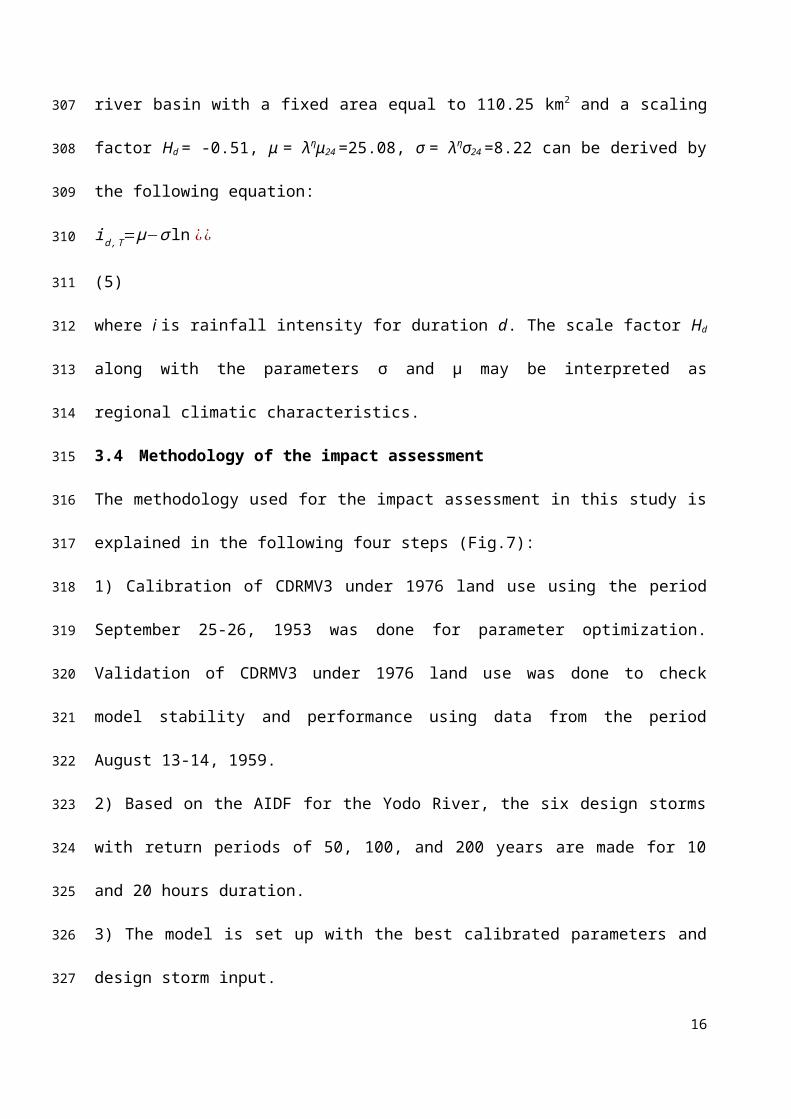
river basin with a fixed area equal to 110.25 km2 and a scaling

factor Hd = -0.51, μ = λημ24 =25.08, σ = λησ24 =8.22 can be derived by

the following equation:

id,T=μ−σln ¿¿

(5)

where i is rainfall intensity for duration d. The scale factor Hd

along with the parameters σ and μ may be interpreted as

regional climatic characteristics.

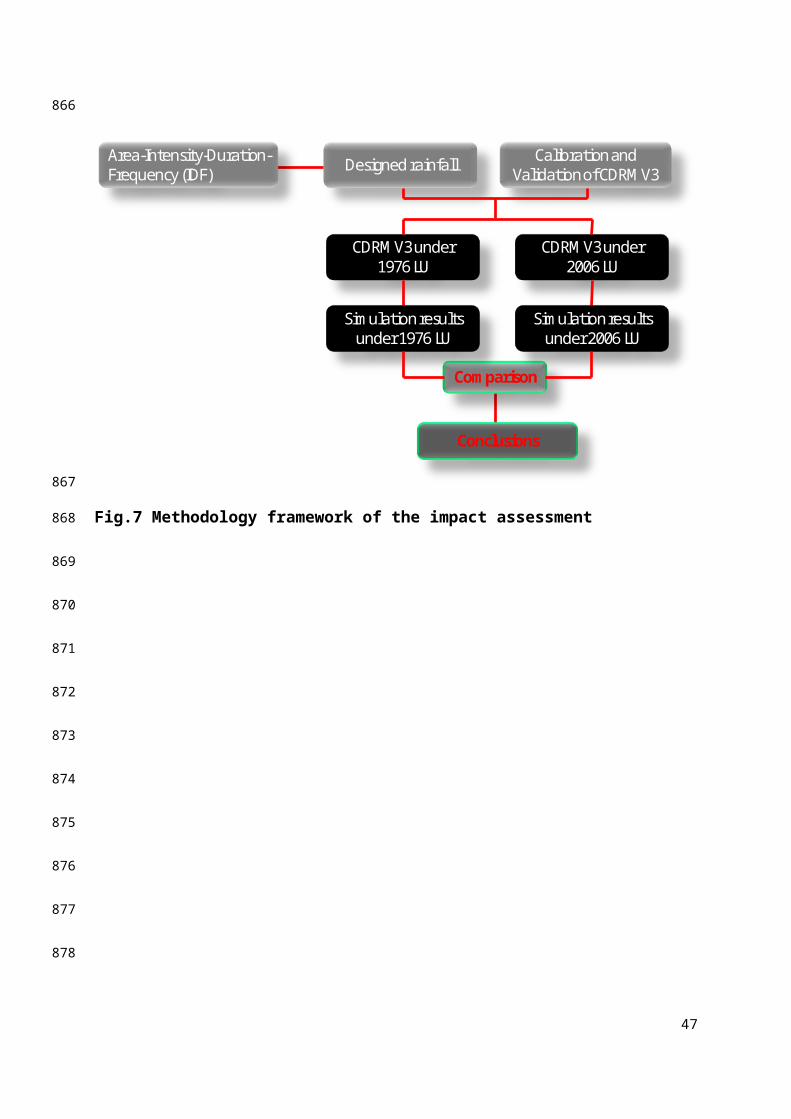
3.4 Methodology of the impact assessment

The methodology used for the impact assessment in this study is

explained in the following four steps (Fig.7):

1) Calibration of CDRMV3 under 1976 land use using the period

September 25-26, 1953 was done for parameter optimization.

Validation of CDRMV3 under 1976 land use was done to check

model stability and performance using data from the period

August 13-14, 1959.

2) Based on the AIDF for the Yodo River, the six design storms

with return periods of 50, 100, and 200 years are made for 10

and 20 hours duration.

3) The model is set up with the best calibrated parameters and

design storm input.

16

307

308

309

310

311

312

313

314

315

316

317

318

319

320

321

322

323

324

325

326

327

4) Simulation results under 1976 and 2006 land use results are

compared.

4. Results and Discussions

4.1 Land use change analysis

We assessed land use change impacts on hydrology between 1976

and 2006. The original classification data of 1976 and 2006

land use is modified for ease of assessing changes. In 1976,

land use type building site A and B are combined into building

site, and lake, marsh, and river area are combined into inland

water area. In the classification of 2006, golf field is

combined with other site. Table 2 shows that forest area

decreased by 0.1% from 1976 to 2006. Building site increased by

3.02% over the same period and rice field and other sites

decreased by 1.69% and 0.77% respectively over the same period.

Table 2 shows that the area of forest decreased by 0.19 km2

from 1976 to 2006, the area of rice field decreased 3.06 km2,

and the area of other site decreased 1.4 km2. All areas showing

decline (rice field, field, forest, waste land, arterial

traffic sites, and other sites) are seen to have contributed to

the land use type ‘building site.’

4.2 Calibration and validation results of the CDRMV3

17

328

329

330

331

332

333

334

335

336

337

338

339

340

341

342

343

344

345

346

347

348

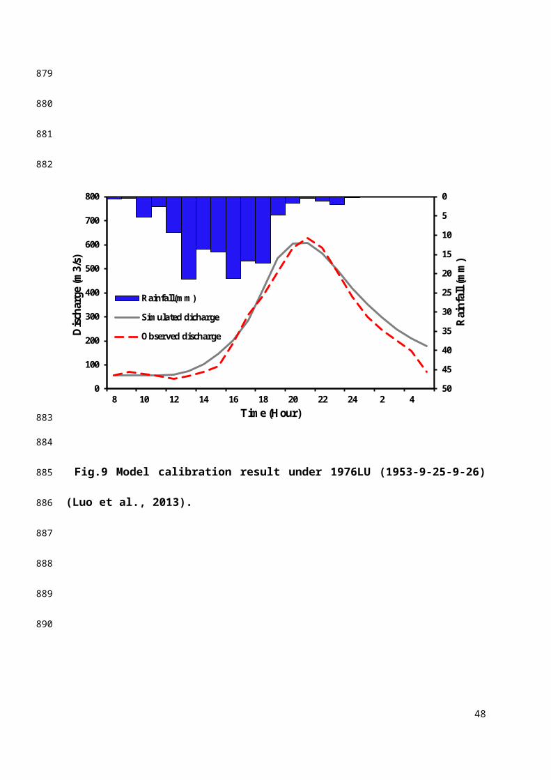
The calibration of the CDRMV3 model is used the rainfall data

from a 1953 flood event due to a lack of observed extreme

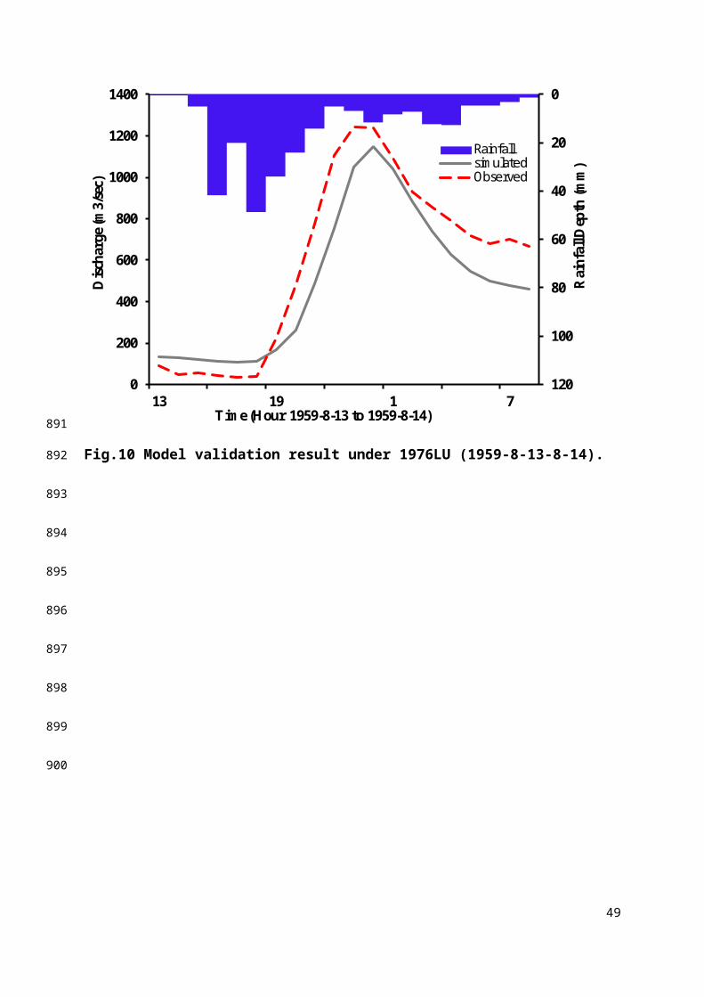
rainfall data from our time period of interest. Fig.9 shows

that the simulation results bracket observed discharge very

well with a NSE of 0.95. The peak discharge of the simulation

is a little lower than the observed discharge. The base flow is

quite fitted with the observed discharge. A detailed

description of the calibration results was presented in Luo et

al. (2014). The observed discharge data from August 13-14,

1959, was used for validation. Fig. 10 shows that the simulated

peak underestimates observed discharge, and the simulated

discharge from 19:00 to 24:00 on August 13 lower than observed

discharge. The simulated discharge from 1:00 to 2:00 on August

14 is quite close to the observed discharge. The simulated

discharge after 3:00 on August 14 shows a significant

decreasing trend. All validation results from August 13-14,

1959, have an NSE of 0.91.

Based on the land use change assessment in 4.1, we

calibrated the significant land use classes, including rice

fields, building sites and other sites, and the forest which

represents the largest land use type in the Kamo River basin.

18

349

350

351

352

353

354

355

356

357

358

359

360

361

362

363

364

365

366

367

368

369

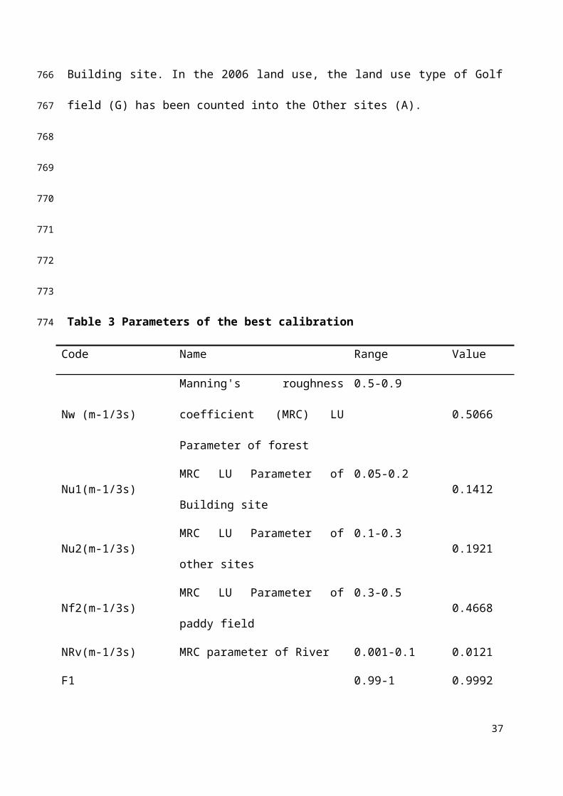
Table 3 shows the values of the best calibration parameters.

The value of Nw is 0.51higher than the value of paddy field

with 0.47.

4.3 Climate condition and land use change effect on extreme

runoff

Land use change assessment was conducted under 1976 and 2006

land use with design storms of different duration, timing,

intensity, and return period. The six design storms of 10 and

20 hours duration with 50, 100 and 200 years return period are

input into the calibrated CDRMV3 for the Kamo River basin. In

this study, we presented the simulated runoff under the six

design storms of 10 hours duration with 50 years return period

considering the land use change impact. Although simulated

runoff under the six design storms of 20 hours duration with

50, 100 and 200 years return period is also calculated, the

results are not included because they are quite similar to

those simulated under the 10 hours duration storm.

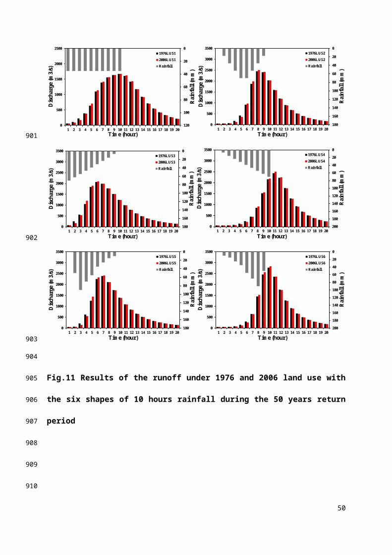
Fig.11 presents the simulated discharge under six design

storms of 10 hours duration with 50 years return period. The

runoff with shape 1 and shape 5 under 2006 land use is lower

than that under 1976 land use in the first 4 hours, and becomes

19

370

371

372

373

374

375

376

377

378

379

380

381

382

383

384

385

386

387

388

389

390

a little higher than that under 1976 land use after the first 4

hours until reaching peak discharge. The most significant

difference in runoff between shape 1 and shape 5 over 1976 to

2006 show that runoff under 2006 land use at the fifth hour is

10.89% and 14.81% higher than that under 1976 land use. The

runoff with shape 3 under 2006 land use is lower than that

under 1976 land use in the first 3 hours, and it is higher than

that under 1976 land use from the fourth hour to the seventh

hour. The runoff with shape 3 under 2006 land use at the fourth

hour is 14.41% greater than that under 1976 land use. The

discharge with shape 4 and 6 under 2006 land use becomes

greater from the second hour to the seventh hour than that in

1976 land use. The peak discharge with shape 4 and shape 6

under 2006 land use is 1.47% and 2.27% higher than that under

1976 land use (Table 4).

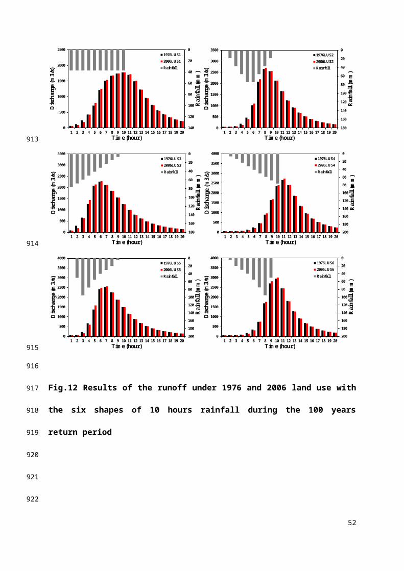
Fig. 12 shows the simulated runoff under the six design

storms of 10 hours duration with 50 years return period. The

peak discharge for shape 1 under 2006 land use is 0.06% higher

than that under 1976 land use, and the runoff for shape 1 under

2006 land use at the fifth hour is 11.67% greater than that

under 1976 land use (Table 4). The runoff with shape 2 under

20

391

392

393

394

395

396

397

398

399

400

401

402

403

404

405

406

407

408

409

410

411

2006 land use is smaller than that under 1976 land use from the

second hour to the fifth hour, and it is higher than that under

1976 land use from the sixth hour to the ninth hour. Peak

discharge with shape 2 under 2006 land use arrives at the

eighth hour with 2706 m3/s which is 2.09% higher than that under

1976 land use (Table 4). The peak discharge with shape 3 under

2006 and 1976 land use arrives at the sixth hour and the peak

discharge with shape 5 under these two land uses is reached at

the seventh hour, and the peak discharge of shape 3 and shape 5

under 2006 are 1.02% and 0.86% respectively higher than that

under 1976 land use (Table 4). The peak discharge with shape 4

and shape 6 under 2006 land use arrive at the same time of the

eleventh hour and the tenth hour with that under 1976 land use,

and it is 1.48% and 1.96% higher than that under 1976 land use.

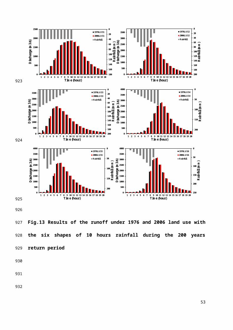
Fig. 13 shows the simulated runoff for the six 200 year

return period design storms under 1976 and 2006 land use. The

peak discharge with shape 1 under 2006 is only 1 m3/s higher

than that under 1976 land use(Table 4), but the simulated

runoff with shape 1 under 2006 land use in the fifth hour is

11.8% higher than that under 1976 land use. The simulated

runoff with shape 2 under 2006 land use is lower than that

21

412

413

414

415

416

417

418

419

420

421

422

423

424

425

426

427

428

429

430

431

432

under 1976 land use from the second hour and the fifth hour,

and it is 8.95% higher at the sixth hour than that under 1976

land use. The simulated discharge with shape 3 and shape 5

under 2006 land use are 13.82% and 15.1% higher at the fourth

and fifth hour with that under 1976 land use. The peak

discharge of shape 4 and shape 6 under 2006 land arrive at the

eleventh hour and the tenth hour with 2839 m3/s and 3173 m3/s

which are 2.64% and 1.7% higher than these under 1976 land use

(Table 4). The changes in peak discharge values for all the

simulations is less than 3% which is considering as the

attribution of the minimal changes on land use from 1976 to

2006.

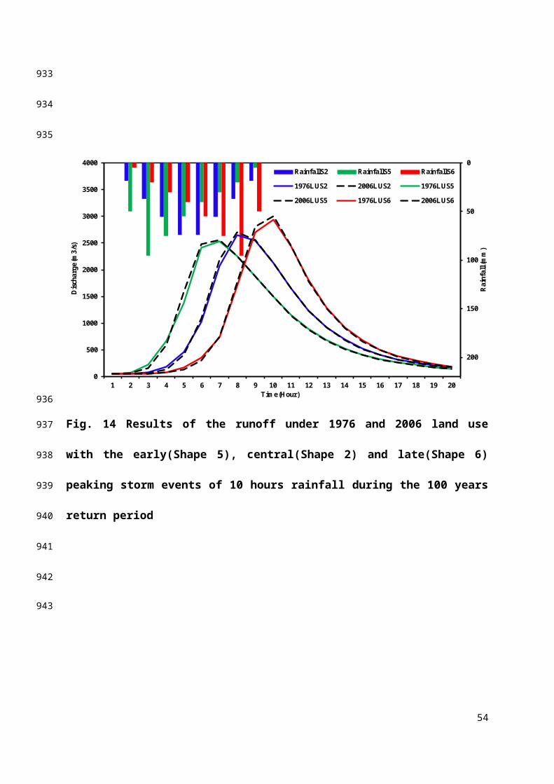
Three synthetic rainfall ‘shapes’ (early-Shape 5, central-

Shape 2 and late-Shape 6 peaking storm events) were selected to

clearly identify the impacts of rainfall shape on hydrological

response. In Fig. 14, the peak discharge under the late

peaking storm is highest with latest peak discharge, while the

peak discharge under the central storm is in the middle between

the peak discharge under the late peaking storm and the early

peaking storm, but it is higher than the peak discharge under

the early peaking storm. Fig.14 shows that the late peaking

22

433

434

435

436

437

438

439

440

441

442

443

444

445

446

447

448

449

450

451

452

453

storm contributes the highest peak discharge, and the peak

discharge under 2006 land-use is significantly higher than the

peak discharge under 1976 land-use.

4.5 Discussion

The designed rainfall with 200 year return period is high

enough that overland flow comes earlier under 2006 land use in

contrast to the situation with 50 and 100 year return period

storms. The runoff of shape 2 with 10 hours duration for these

three return periods under 2006 land use shows lower discharge

from the second hour to the fifth hour than those under 1976

land use, and the highest percentage of the runoff distance

between these in 2006 and 1976 are found at the fourth hour

with 28%, 29% and 30%. The runoff of shape 3 and shape 5 under

2006 land use show significantly higher values in the fourth

hour and the fifth hour than 1976 land use. The runoff of shape

6 shows a significant difference between 2006 and 1976 land use

in times before peak discharge.

Based on the assessment of the runoff with 10 and 20 hours

duration, and six design storms for 50, 100 and 200 year return

periods, the runoff for all events under 2006 land use is a

little lower in the first few hours and a little higher in the

23

454

455

456

457

458

459

460

461

462

463

464

465

466

467

468

469

470

471

472

473

474

few hours before arrival of peak discharge than those under

1976 land use. The main reason for this is that water storage

in 2006 land use is lower before the flood events, and overland

flow is conveyed to the outlet more easily than that in 1976

land use due to the large urban area and less forest area in

2006 land use. The runoff of shape 3 with 10 and 20 hours

duration in the 50, 100 and 200 years return periods show that

discharge increased very quickly and reached peak discharge

within six or seven hours due to the high input rainfall in the

first few hours. The runoff of shape 5 with 10 and 20 hours

duration in the 50, 100 and 200 years return periods show that

it increased very early but a little slower than for shape 3,

and the peak discharge is higher than in the case of shape 3.

Compared with the runoff under the six designed rainfall

shapes, the runoff of shape 6 gave the highest peak discharge

and is considered the most dangerous flood event. The impacts

of rainfall shape on river discharge and implications for flood

management are elucidated via the results of simulations using

early, central and late peaking storm events.

Based on the recent Intergovernmental Panel on Climate

Change (IPCC) Assessment Report (IPCC 2007), using the

24

475

476

477

478

479

480

481

482

483

484

485

486

487

488

489

490

491

492

493

494

495

assessment of future climate from a number of global climate

models (GCM) with different emission scenarios, trends in

extreme precipitation events are expected to increase. The

historical Area IDF has been modified by considering the

relationship between the historical and future climate

conditions (Zhu J., 2013). The historical Area IDF and dynamic

character should be considered into scenario estimation of

extreme runoff under the future climate condition.

5. Conclusions

Land use change impact assessment on runoff is a key

approach for policies makers and scientists in urban planning

and flood risk management. We assessed the impact of land use

change between 1976 and 2006 on runoff generated by design

extreme rainfall of 10 and 20 hours duration with six distinct

intensities and duration and 50, 100 and 200 years return

periods. The runoff of all the cases under 2006 land use is

higher than under 1976 land use due to the larger urban area

and the lower coverage of forest area compared to the 1976 land

use case. However, minimal changes in the land-cover class

occupying the largest land area are actually responsible for

very small changes in flood magnitudes. We found that shape 3

25

496

497

498

499

500

501

502

503

504

505

506

507

508

509

510

511

512

513

514

515

516

leads to extremely fast peak discharge, as does shape 5 and

shape 6 discharge increases slowly, but can lead to the highest

peak discharge. Runoff under 2006 land use gave a higher

discharge than these under 1976 land use, and the shape 6 is

the most dangerous designed rainfall for the future urban

planning and flood risk management. The results of the

hydrological model simulation using the historical Area IDF are

essential to find the impact of rainfall shape and the human

activities impact on river discharge. The results of this study

also provide the designed hourly extreme runoff under the

extreme rainfall from the historical Area IDF for the further

researches on predicting a hourly inundation condition under

the extreme events. To considering the climate change for Area

IDF, it is necessary to study the change on Area IDF by using

the adjustment factor. The adjustment factor is utilized from

the historical recorded rainfall and the future scenarios from

the output of a number of Global Climate Models (GCMs) based on

the assumptive relationship between the historical rainfall and

the future rainfall.

It is important to note that there are several limitations

to this study. Changes in hourly precipitation patterns may be

26

517

518

519

520

521

522

523

524

525

526

527

528

529

530

531

532

533

534

535

536

537

significantly more complex than those used in the study. More

complex patterns have been neglected here and a more

comprehensive study should investigate more nuanced hydrologic

response. Changes in rainfall intensity outside the range

projected by Naht et al. 2007 have been neglected. Naht et al.

use 1956-1985 to formulate equations to estimate rainfall

intensities. However, precipitation dynamics have changed

significantly in the past ~25 years due to climate change.

Finally changes in antecedent soil-moisture were unchanged

between the two durations. All of these limitations speak to

the complexity of the problem of land-use change and hydrologic

forecasting. Future work should build on what is presented here

by adding realistic nuances in land-use change and in synthetic

design storms.

Acknowledgement

The fiscal supports in this study were provided by the project

on “Water and Urban Initiative” at the United Nations

University - Institute for the Advanced Study of Sustainability

(UNU-IAS), the Japan Institute of Country-ology and Engineering

(JICE) Grant Number 13003, the JSPS Grant-in-Aid for Scientific

Research (A) Grant Number 24248041, and Inter-Graduate School

27

538

539

540

541

542

543

544

545

546

547

548

549

550

551

552

553

554

555

556

557

558

Program for Sustainable Development and Survivable Societies

(GSS), MEXT Program for Leading Graduate Schools 2011-2018.

References

Apip, Sayama, T., Tachikawa, Y., and Takara, K., 2012. Spatial

lumping of a distributed rainfall sediment runoff model and

effective lumping scale, Hydrological Processes, Volume

26(6), 855–871.

Bell, F. C., 1969. Generalized rainfall duration frequency

relationships. Journal of Hydraulic Div., ASCE, 95(1), 311-327.

Benito, G., Rico, M., Sánchez-Moya, Y., Sopeña, A.,

Thorndycraft, Barriendos, V.R., M., 2010. The impact of late

Holocene climatic variability and land use change on the flood

hydrology of the Guadalentín River, southeast Spain. Global and

Planetary Change 70, 53–63.

Brath, A., Montanari, A., Moretti, G., 2006. Assessing the

effect on flood frequency of land use change via hydrological

simulation (with uncertainty). Journal of Hydrology 324 (1–4),

141–153.

Chen, C. L., 1983. Rainfall intensity duration frequency

formulas, Journal of Hydraulic Engineering, ASCE, 109(12),

28

559

560

561

562

563

564

565

566

567

568

569

570

571

572

573

574

575

576

577

578

579

1603-1621.

Chow, V.T., Maidment, D.R. & Mays, L.W, 1988. Applied

Hydrology, McGraw-Hill.

Costa, M.H., Botta, A., Cardille, J.A., 2003. Effects of large-

scale changes in land cover on the discharge of the Tocantins

River, Southeastern Amazonia. Journal of Hydrology 283, 206–

217.

Crooks, S., Davies, H., 2001. Assessment of land use change in

the Thames catchment and its effect on the flood regime of the

river. Physics and Chemistry of the Earth, Part B 26 (7–8),

583–591.

De Roo, A., Odijk, M., Schmuck, G., Koster, E., Lucieer, A.,

2001. Assessing the effects of land use changes on floods in

the Meuse and Oder catchment. Physics and Chemistry of the

Earth, Part B 26 (7), 593–599.

Dunn, S.M., Mackay, R., 1995. Spatial variation in

evapotranspiration and the influence of land use on catchment

hydrology, Journal of Hydrology 171, 49-73.

Hershfied, D. M., 1961. Estimating the Probable Maximum

Precipitation, Journal of the Hydraulic Division, Proceeding of

the ASCE, HY5, 99-116.

29

580

581

582

583

584

585

586

587

588

589

590

591

592

593

594

595

596

597

598

599

600

Kojima, T. 1997. Application of remote sensing and GIS to

hydrological analysis. Doctorate of Engineering Dissertation,

Kyoto University, Japan (in Japanese).

Kothyari, U. C. and Grade, R.J.. 1992. Rainfall intensity

duration frequency formula for India, J. Hydr. Eng., ASCE,

118(2), 323-336.

Koutsoyiannis, D., Manetas, A., 1998. A mathematical framework

for studying rainfall intensity duration frequency

relationships, Journal of Hydrology, 206, 118–135.

Luo P., Takara, K., APIP, He, B. and Nover, D., 2014. Paleoflood

simulation in the kamo river basin by using a grid-cell

distributed rainfall-runoff model, Journal of Flood Risk

Management. Vol.15, pp.1052–1061.

Nhat, L. M., Tachikawa, Y., Takara, K.. 2006. Establishment of

Intensity-Duration-Frequency curves for precipitation in the

monsoon area of Vietnam, Annuals of Disas. Prev. Res. Inst.,

Kyoto Univ., No. 49B.

Nhat , L. M. , Tachikawa,Y., Sayama, T. and Takara, K., 2007. A

simple scaling characteristics of rainfall in time and space to

derive intensity duration frequency relationships. Annual

Journal of Hydraulic Engineering, JSCE, Vol.51, 73-78.

30

601

602

603

604

605

606

607

608

609

610

611

612

613

614

615

616

617

618

619

620

621

Sayama, T., Takara, K., Tachikawa, Y., 2003. Reliability

evaluation of rainfall-sediment-runoff models, Erosion

Prediction in Ungauged Basins: Integrating Methods and

Techniques (Proceedings of symposium HS01 held during IUGG2003

at Sapporo, July 2003). IAHS Publ. no. 279. 131-141.

Siriwardena, L., Finlayson, B.L., McMahon, T.A., 2006. The

impact of land use change on catchment hydrology in large

catchments: The Comet River, Central Queensland, Australia.

Journal of Hydrology 326, 199–214.

Svensson, C., Clarke, R. T., Jones, D. A., 2007. An

experimental comparison of methods for estimating rainfall

intensity-duration-frequency relations from fragmentary

records. Journal of Hydrology 341, 79– 89

Van Nguyen, V. T., Nguyen, T.-D., Ashkar, F., 2002. Regional

frequency analysis of extreme rainfalls, Water Sci. Technol.

45(2), 75–81.

Wang, G.X., Zhang, Y., Liu, G.M., Chen, L., 2006. Impact of

land-use change on hydrological processes in the Maying River

basin, China. Science in China Series D: Earth Sciences 49

(10), 1098–1110.

Ward, P.J., Renssen, H., Aerts, J.C.J.H., van Balen R.T., and

31

622

623

624

625

626

627

628

629

630

631

632

633

634

635

636

637

638

639

640

641

642

Vandenberghe, J., 2008. Strong increases in flood frequency and

discharge of the River Meuse over the late Holocene: impacts of

long-term anthropogenic land use change and climate

variability, Hydrol. Earth Syst. Sci., Vol. 12, 159–175.

White, M. D., Greer, K. A., 2006. The effects of watershed

urbanization on the stream hydrology and riparian vegetation of

Los Pe˜nasquitos Creek, California, Landscape and Urban

Planning 74, 125–138

Wijesekara, G.N., Gupta, A., Valeo, C., Hasbani, J.-G., Qiao,

Y., Delaney, P., Marceau, D.J., 2012. Assessing the impact of

future land-use changes on hydrological processes in the Elbow

River watershed in southern Alberta, Canada. Journal of

Hydrology, Volumes 412–413, 220–232

Zhu, J. (2013). ”Impact of Climate Change on Extreme Rainfall

across the United States.” J. Hydrol. Eng., 18(10), 1301–1309.

Intergovernmental Panel on Climate Change (IPCC). (2007).

“Climate change 2007: Synthesis report, summary for

policymakers.” http://⟨

www.ipcc.ch/pdf/assessment-report/ar4/syr/ar4_syr_spm.pdf⟩

(October 29, 2013).

Luo P., Takara, K., APIP, He, B., and Nover, D., 2014a.

32

643

644

645

646

647

648

649

650

651

652

653

654

655

656

657

658

659

660

661

662

663

Reconstruction assessment of historical land use: a case study

at the Kamo River basin, Kyoto, Japan, Computers & Geosciences

63, 106–115.

Luo P., He, B., Takara, K., Duan, W., APIP, Nover, D.,

Watanabe, T., Hu, M., Nakagami K., and Takamiya, I., 2014b.

Assessment of paleo-hydrology and paleo-inundation conditions:

the process, Procedia Environmental Science 20, pp. 747-752.

Luo P., He, B. Takara, K., Xiong, Y. E., Nover, D., Duan, W.,

and Fukushi, K., 2015. Historical Assessment of Chinese and

Japanese Flood Management Policies and Implications for

Managing Future Floods, Environmental Science & Policy, Vol. 48,

pp. 265-277.

33

664

665

666

667

668

669

670

671

672

673

674

675

676

677

678679680681682683684685686687688689690691692693694695

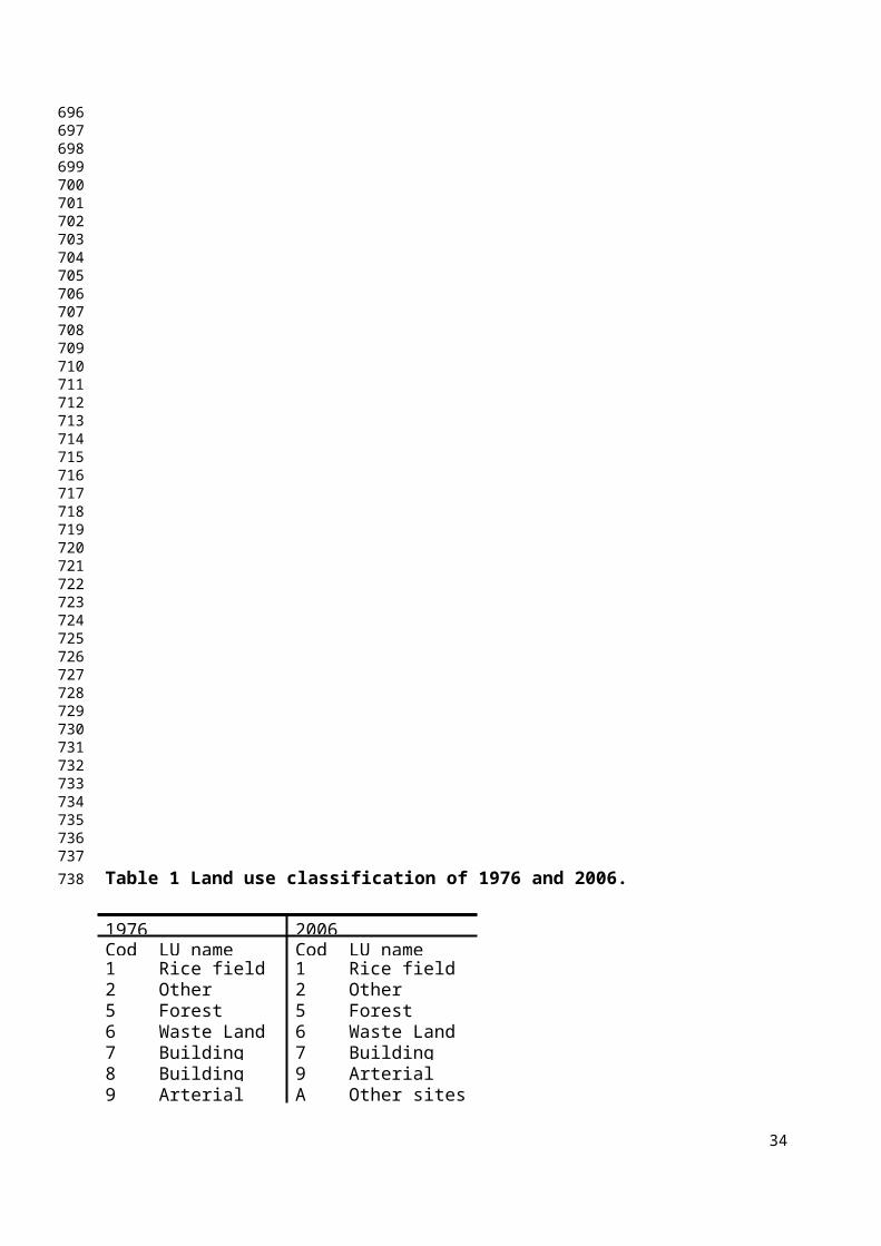
Table 1 Land use classification of 1976 and 2006.

1976 2006Cod LU name Cod LU name1 Rice field 1 Rice field2 Other 2 Other5 Forest 5 Forest6 Waste Land 6 Waste Land7 Building 7 Building8 Building 9 Arterial9 Arterial A Other sites

34

696697698699700701702703704705706707708709710711712713714715716717718719720721722723724725726727728729730731732733734735736737738

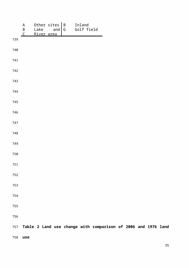
A Other sites B InlandB Lake and G Golf fieldC River area

Table 2 Land use change with comparison of 2006 and 1976 land

use

35

739

740

741

742

743

744

745

746

747

748

749

750

751

752

753

754

755

756

757

758

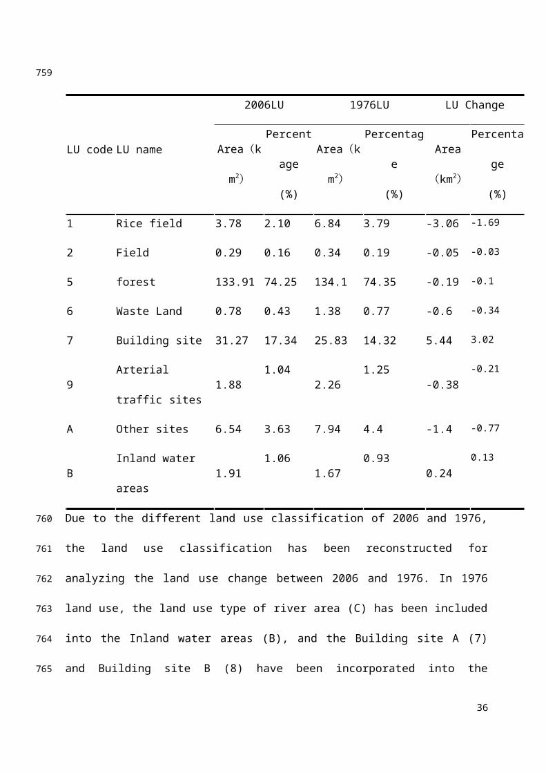
LU code LU name

2006LU 1976LU LU Change

Area（k

m2）

Percent

age

(%)

Area（k

m2）

Percentag

e

(%)

Area

（km2）

Percenta

ge

(%)

1 Rice field 3.78 2.10 6.84 3.79 -3.06 -1.69

2 Field 0.29 0.16 0.34 0.19 -0.05 -0.03

5 forest 133.91 74.25 134.1 74.35 -0.19 -0.1

6 Waste Land 0.78 0.43 1.38 0.77 -0.6 -0.34

7 Building site 31.27 17.34 25.83 14.32 5.44 3.02

9Arterial

traffic sites1.88

1.042.26

1.25-0.38

-0.21

A Other sites 6.54 3.63 7.94 4.4 -1.4 -0.77

BInland water

areas1.91

1.061.67

0.930.24

0.13

Due to the different land use classification of 2006 and 1976,

the land use classification has been reconstructed for

analyzing the land use change between 2006 and 1976. In 1976

land use, the land use type of river area (C) has been included

into the Inland water areas (B), and the Building site A (7)

and Building site B (8) have been incorporated into the

36

759

760

761

762

763

764

765

Building site. In the 2006 land use, the land use type of Golf

field (G) has been counted into the Other sites (A).

Table 3 Parameters of the best calibration

Code Name Range Value

Nw (m-1/3s)

Manning's roughness

coefficient (MRC) LU

Parameter of forest

0.5-0.9

0.5066

Nu1(m-1/3s)MRC LU Parameter of

Building site

0.05-0.20.1412

Nu2(m-1/3s)MRC LU Parameter of

other sites

0.1-0.30.1921

Nf2(m-1/3s)MRC LU Parameter of

paddy field

0.3-0.50.4668

NRv(m-1/3s) MRC parameter of River 0.001-0.1 0.0121

F1 0.99-1 0.9992

37

766

767

768

769

770

771

772

773

774

ASOU (mm) Total soil depth 100-500 105.4310

TOUSUIMS(mm s-

1)

Hydraulic conductivity

in saturated layer

0.0001-0.0020.0004

BetacParameter for

unsaturated flow

3.0-10.06.8597

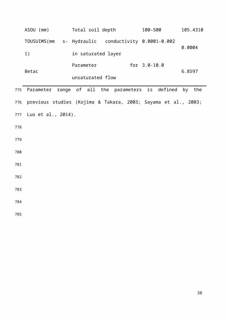
Parameter range of all the parameters is defined by the

previous studies (Kojima & Takara, 2003; Sayama et al., 2003;

Luo et al., 2014).

38

775

776

777

778

779

780

781

782

783

784

785

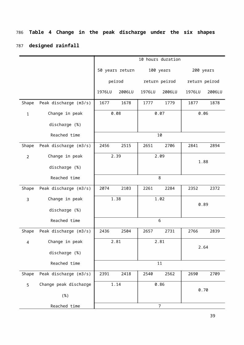
Table 4 Change in the peak discharge under the six shapes

designed rainfall

10 hours duration

50 years return

peirod

100 years

return peirod

200 years

return peirod

1976LU 2006LU 1976LU 2006LU 1976LU 2006LU

Shape

1

Peak discharge (m3/s) 1677 1678 1777 1779 1877 1878

Change in peak

discharge (%)

0.08 0.07 0.06

Reached time 10

Shape

2


Change in peak

discharge (%)

2.39 2.091.88

Reached time 8

Shape

3


Change in peak

discharge (%)

1.38 1.020.89

Reached time 6

Shape

4


Change in peak

discharge (%)

2.81 2.812.64

Reached time 11

Shape

5


Change peak discharge

(%)

1.14 0.860.70

Reached time 7

39

786

787

Shape

6


Change peak discharge

(%)

2.29 1.961.70

Reached time 10

Fig.1 The location and DEM map of Kamo River basin

40

788

789

790

791

792

793

794

795

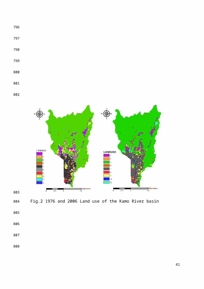
Fig.2 1976 and 2006 Land use of the Kamo River basin

41

796

797

798

799

800

801

802

803

804

805

806

807

808

0102030405060708090100

1 2 3 4 5 6 7 8 9 10

Rainfall (mm)

Duration (hour)

Shape5

0102030405060708090100

1 2 3 4 5 6 7 8 9 10

Rainfall (mm)

Duration (hour)

Shape6

0102030405060708090100

1 2 3 4 5 6 7 8 9 10

Rainfall (mm)

Duration (hour)

Shape3

0102030405060708090100

1 2 3 4 5 6 7 8 9 10

Rainfall (mm)

Duration (hour)

Shape4

0102030405060708090100

1 2 3 4 5 6 7 8 9 10

Rainfall (mm)

Duration (hour)

Shape2

0102030405060708090100

1 2 3 4 5 6 7 8 9 10

Rainfall (mm)

Duration (hour)

Shape1

Fig.3 Six shapes of AIDF designed rainfall

42

809

810

811

812

813

814

815

816

817

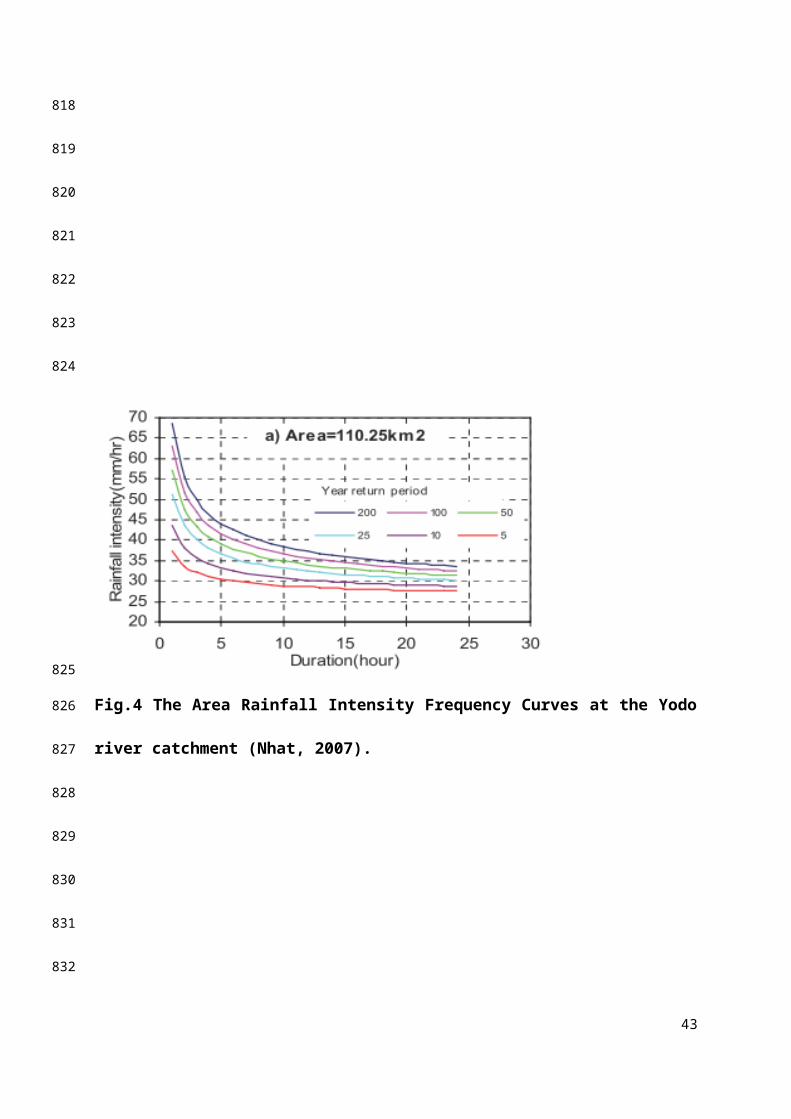
Fig.4 The Area Rainfall Intensity Frequency Curves at the Yodo

river catchment (Nhat, 2007).

43

818

819

820

821

822

823

824

825

826

827

828

829

830

831

832

qh

D

rda

dm

x

L

qh

D

rda

dm

x

L

44

(b)

(a)

833

834

835

836

837

838

839

840

841

842

843

dm

h

q

)/( mmm dhdvq

)( mamm dhvdvq

mamamm dhdhvdvq )()(

dadm

qm

qaNon-capillary subsurface flow

Soil (Solid)

Surface flowda

D

a

mCapillary subsurface flow

dm

h

q

)/( mmm dhdvq

)( mamm dhvdvq


dadm

qm


Soil (Solid)

Surface flowda

D

a


h

q

)/( mmm dhdvq

)( mamm dhvdvq


dadm

qm


Soil (Solid)

Surface flowda

D

a


Figure 5. The surface and sub surface model structure (a)

and the width discharge and water depth (q-h) in each

grid (b) (Apip et al., 2010).

45

844

845

846

847

848

849

850

851

852

853

854

855

Ensem ble Stream Flow Sim ulation

Rejection of m odel Results (NSE ≥0.75)

Best m odel perform anceParam etric Uncertainty

M odel perform ance m easurem ent

Observed Stream Flow

Fig.6 Framework of the Monte Carlo approach (MCA)

46

856

857

858

859

860

861

862

863

864

865

CDRM V3 under 1976 LU

Designed rainfall

Com parison

Area-Intensity-Duration-Frequency (IDF)

CDRM V3 under 2006 LU

Calibration and Validation of CDRM V3

Sim ulation results under 1976 LU

Sim ulation results under 2006 LU

Conclusions

Fig.7 Methodology framework of the impact assessment

47

866

867

868

869

870

871

872

873

874

875

876

877

878

0

5

10

15

20

25

30

35

40

45

500

100

200

300

400

500

600

700

800

8 10 12 14 16 18 20 22 24 2 4

Rainfall (mm)

Discharge (m3/s)

Tim e (H our)

Rainfall(m m )

Sim ulated dicharge

Observed discharge

Fig.9 Model calibration result under 1976LU (1953-9-25-9-26)

(Luo et al., 2013).

48

879

880

881

882

883

884

885

886

887

888

889

890

0

20

40

60

80

100

1200

200

400

600

800

1000

1200

1400

13 19 1 7

Rainfall D

epth (m

m)

Discharge (m3/sec)

Tim e (Hour 1959-8-13 to 1959-8-14)

Rainfallsim ulatedObserved

Fig.10 Model validation result under 1976LU (1959-8-13-8-14).

49

891

892

893

894

895

896

897

898

899

900

0

20

40

60

80

100

1200

500

1000

1500

2000

2500

1 2 3 4 5 6 7 8 9 10 11 12 13 14 15 16 17 18 19 20

Rainfall (mm)

Discharge (m3/s)

Tim e (hour)

1976LUS12006LUS1Rainfall

0

20

40

60

80

100

120

140

160

1800

500

1000

1500

2000

2500

3000

3500

1 2 3 4 5 6 7 8 9 10 11 12 13 14 15 16 17 18 19 20

Rainfall (mm)

Discharge (m3/s)

Tim e (hour)


0

20

40

60

80

100

120

140

160

1800

500

1000

1500

2000

2500

3000

3500

1 2 3 4 5 6 7 8 9 10 11 12 13 14 15 16 17 18 19 20

Rainfall (mm)

Discharge (m3/s)

Tim e (hour)


020

4060

80100120

140160

1802000

500

1000

1500

2000

2500

3000

3500

1 2 3 4 5 6 7 8 9 10 11 12 13 14 15 16 17 18 19 20

Rainfall (mm)

Discharge (m3/s)

Tim e (hour)


0

20

40

60

80

100

120

140

160

1800

500

1000

1500

2000

2500

3000

3500

1 2 3 4 5 6 7 8 9 10 11 12 13 14 15 16 17 18 19 20

Rainfall (mm)

Discharge (m3/s)

Tim e (hour)


0

20

40

60

80

100

120

140

160

180

2000

500

1000

1500

2000

2500

3000

3500

1 2 3 4 5 6 7 8 9 10 11 12 13 14 15 16 17 18 19 20

Rainfall (mm)

Discharge (m3/s)

Tim e (hour)


Fig.11 Results of the runoff under 1976 and 2006 land use with

the six shapes of 10 hours rainfall during the 50 years return

period

50

901

902

903

904

905

906

907

908

909

910

51

911

912

0

20

40

60

80

100

120

1400

500

1000

1500

2000

2500

1 2 3 4 5 6 7 8 9 10 11 12 13 14 15 16 17 18 19 20

Rainfall (mm)

Discharge (m3/s)

Tim e (hour)


0

20

40

60

80

100

120

140

160

1800

500

1000

1500

2000

2500

3000

3500

1 2 3 4 5 6 7 8 9 10 11 12 13 14 15 16 17 18 19 20

Rainfall (mm)

Discharge (m3/s)

Tim e (hour)


0

20

40

60

80

100

120

140

160

1800

500

1000

1500

2000

2500

3000

3500

1 2 3 4 5 6 7 8 9 10 11 12 13 14 15 16 17 18 19 20

Rainfall (mm)

Discharge (m3/s)

Tim e (hour)


0

20

40

60

80

100

120

140

160

180

2000

500

1000

1500

2000

2500

3000

3500

4000

1 2 3 4 5 6 7 8 9 10 11 12 13 14 15 16 17 18 19 20

Rainfall (mm)

Discharge (m3/s)

Tim e (hour)


0

20

40

60

80

100

120

140

160

180

2000

500

1000

1500

2000

2500

3000

3500

4000

1 2 3 4 5 6 7 8 9 10 11 12 13 14 15 16 17 18 19 20

Rainfall (mm)

Discharge (m3/s)

Tim e (hour)


0

20

40

60

80

100

120

140

160

180

2000

500

1000

1500

2000

2500

3000

3500

4000

1 2 3 4 5 6 7 8 9 10 11 12 13 14 15 16 17 18 19 20

Rainfall (mm)

Discharge (m3/s)

Tim e (hour)



the six shapes of 10 hours rainfall during the 100 years

return period

52

913

914

915

916

917

918

919

920

921

922

0

20

40

60

80

100

120

140

160

1800

500

1000

1500

2000

2500

1 2 3 4 5 6 7 8 9 10 11 12 13 14 15 16 17 18 19 20

Rainfall (mm)

Discharge (m3/s)

Tim e (hour)


020

4060

80100120

140160

1802000

500

1000

1500

2000

2500

3000

3500

1 2 3 4 5 6 7 8 9 10 11 12 13 14 15 16 17 18 19 20

Rainfall (mm)

Discharge (m3/s)

Tim e (hour)


0

20

40

60

80100

120

140

160

180

2000

500

1000

1500

2000

2500

3000

3500

1 2 3 4 5 6 7 8 9 10 11 12 13 14 15 16 17 18 19 20

Rainfall (mm)

Discharge (m3/s)

Tim e (hour)


0

50

100

150

2000

500

1000

1500

2000

2500

3000

3500

4000

1 2 3 4 5 6 7 8 9 10 11 12 13 14 15 16 17 18 19 20

Rainfall (mm)

Discharge (m3/s)

Tim e (hour)


0

50

100

150

2000

500

1000

1500

2000

2500

3000

3500

4000

1 2 3 4 5 6 7 8 9 10 11 12 13 14 15 16 17 18 19 20

Rainfall (mm)

Discharge (m3/s)

Tim e (hour)


0

50

100

150

200

2500

500

1000

1500

2000

2500

3000

3500

4000

1 2 3 4 5 6 7 8 9 10 11 12 13 14 15 16 17 18 19 20Ra

infall (mm)

Discharge (m3/s)

Tim e (hour)



the six shapes of 10 hours rainfall during the 200 years

return period

53

923

924

925

926

927

928

929

930

931

932

0

50

100

150

200

0

500

1000

1500

2000

2500

3000

3500

4000

1 2 3 4 5 6 7 8 9 10 11 12 13 14 15 16 17 18 19 20

Rainfall (mm)

Discharge (m3/s)

Tim e (Hour)

RainfallS2 RainfallS5 RainfallS6

1976LUS2 2006LUS2 1976LUS5

2006LUS5 1976LUS6 2006LUS6

Fig. 14 Results of the runoff under 1976 and 2006 land use

with the early(Shape 5), central(Shape 2) and late(Shape 6)

peaking storm events of 10 hours rainfall during the 100 years

return period

54

933

934

935

936

937

938

939

940

941

942

943

Impact assessment of rainfall scenarios and land-use change on hydrologic response using synthetic Area IDF curves

Documents