Immunological Bioinformatics

Welcome message from author
This document is posted to help you gain knowledge. Please leave a comment to let me know what you think about it! Share it to your friends and learn new things together.
Transcript

Immunological Bioinformatics

Sorin Istrail, Pavel Pevzner, and Michael Waterman, editors
Computational molecular biology is a new discipline, bringing togethercomputational, statistical, experimental, and technological methods, which isenergizing and dramatically accelerating the discovery of new technologiesand tools for molecular biology. The MIT Press Series on ComputationalMolecular Biology is intended to provide a unique and effective venue forthe rapid publication of monographs, textbooks, edited collections, referenceworks, and lecture notes of the highest quality.
Computational Molecular Biology: An Algorithmic ApproachPavel A. Pevzner, 2000
Computational Methods for Modeling Biochemical NetworksJames M. Bower and Hamid Bolouri, editors, 2001
Current Topics in Computational Molecular BiologyTao Jiang, Ying Xu, and Michael Q. Zhang, editors, 2002
Gene Regulation and Metabolism: Postgenomic Computation ApproachesJulio Collado-Vides, editor, 2002
Microarrays for an Integrative GenomicsIsaac S. Kohane, Alvin Kho, and Atul J. Butte, 2002
Kernel Methods in Computational BiologyBernhard Schölkopf, Koji Tsuda and Jean-Philippe Vert, editors, 2004
An Introduction to Bioinformatics AlgorithmsNeil C. Jones and Pavel A. Pevzner, 2004
Immunological BioinformaticsOle Lund, Morten Nielsen, Claus Lundegaard, Can Kesmir and Søren Brunak,2005
Ontologies for BioinformaticsKenneth Baclawski and Tianhua Niu, 2005

Immunological Bioinformatics
Ole LundMorten NielsenClaus LundegaardCan KesmirSøren Brunak
The MIT PressCambridge, MassachusettsLondon, England

c©2005 Massachusetts Institute of Technology
All rights reserved. No part of this book may be reproduced in any formby any electronic or mechanical means (including photocopying, recording,or information storage and retrieval) without permission in writing from thepublisher.
MIT press books may be purchased at special quantity discounts forbusiness or sales promotional use. For information please email [email protected] or write to Special Sales Department, The MITpress, 55 Hayward Street, Cambridge, MA 02142.
This book was set in Lucida by the authors and was printed and bound in theUnited States of America.
Library of Congress Cataloging-in-Publication Data
Immunological bioinformatics / Ole Lund .. [et al.].p. cm. — (Computational molecular biology)
Includes bibliographical references and index.ISBN 0-262-12280-4 (alk. paper)1. Immunoinformatics. I. Lund, Ole. II. Series.QR182.2.I46I465 2005571.9’6’0285-dc22
2005042806

Contents
Preface ix
1 Immune Systems and Systems Biology 11.1 Innate and Adaptive Immunity in Vertebrates 101.2 Antigen Processing and Presentation 111.3 Individualized Immune Reactivity 14
2 Contemporary Challenges to the Immune System 172.1 Infectious Diseases in the New Millennium 172.2 Major Killers in the World 172.3 Childhood Diseases 202.4 Clustering of Infectious Disease Organisms 222.5 Biodefense Targets 282.6 Cancer 302.7 Allergy 302.8 Autoimmune Diseases 31
3 Sequence Analysis in Immunology 333.1 Sequence Analysis 333.2 Alignments 343.3 Multiple Alignments 503.4 DNA Alignments 523.5 Molecular Evolution and Phylogeny 533.6 Viral Evolution and Escape: Sequence Variation 553.7 Prediction of Functional Features of Biological Sequences 59
4 Methods Applied in Immunological Bioinformatics 674.1 Simple Motifs, Motifs and Matrices 674.2 Information Carried by Immunogenic Sequences 704.3 Sequence Weighting Methods 734.4 Pseudocount Correction Methods 75
v

vi Contents
4.5 Weight on Pseudocount Correction 774.6 Position Specific Weighting 774.7 Gibbs Sampling 784.8 Hidden Markov Models 824.9 Artificial Neural Networks 894.10 Performance Measures for Prediction Methods 974.11 Clustering and Generation of Representative Sets 100
5 DNA Microarrays in Immunology 1015.1 DNA Microarray Analysis 1015.2 Clustering 1045.3 Immunological Applications 106
6 Prediction of Cytotoxic T Cell (MHC Class I) Epitopes 1096.1 Background and Historical Overview of Methods for Pep-
tide MHC Binding Prediction 1106.2 MHC Class I Epitope Binding Prediction Trained on Small
Data Sets 1126.3 Prediction of CTL Epitopes by Neural Network Methods 1186.4 Summary of the Prediction Approach 131
7 Antigen Processing in the MHC Class I Pathway 1337.1 The Proteasome 1337.2 Evolution of the Immunosubunits 1357.3 Specificity of the (Immuno)Proteasome 1377.4 Predicting Proteasome Specificity 1417.5 Comparison of Proteasomal Prediction Performance 1457.6 Escape from Proteasomal Cleavage 1477.7 Post-Proteasomal Processing of Epitopes 1487.8 Predicting the Specificity of TAP 1517.9 Proteasome and TAP Evolution 152
8 Prediction of Helper T Cell (MHC Class II) Epitopes 1558.1 Prediction Methods 1568.2 The Gibbs Sampler Method 1578.3 Further Improvements of the Approach 170
9 Processing of MHC Class II Epitopes 1739.1 Enzymes Involved in Generating MHC Class II Ligands 1749.2 Selective Loading of Peptides to MHC Class II Molecules 1779.3 Phylogenetic Analysis of the Lysosomal Proteases 1789.4 Signs of the Specificities of Lysosomal Proteases on MHC
Class II Epitopes 180

Contents vii
9.5 Predicting the Specificity of Lysosomal Enzymes 180
10 B Cell Epitopes 18510.1 Affinity Maturation 18610.2 Recognition of Antigen by B cells 18910.3 Neutralizing Antibodies 199
11 Vaccine Design 20111.1 Categories of Vaccines 20211.2 Polytope Vaccine: Optimizing Plasmid Design 20511.3 Therapeutic Vaccines 20711.4 Vaccine Market 211
12 Web-Based Tools for Vaccine Design 21312.1 Databases of MHC Ligands 21312.2 Prediction Servers 215
13 MHC Polymorphism 22113.1 What Causes MHC Polymorphism? 22113.2 MHC Supertypes 223
14 Predicting Immunogenicity: An Integrative Approach 24114.1 Combination of MHC and Proteasome Predictions 24214.2 Independent Contributions from TAP and Proteasome
Predictions 24314.3 Combinations of MHC, TAP, and Proteasome Predictions 24514.4 Validation on HIV Data Set 24914.5 Perspectives on Data Integration 250
References 252

viii Contents
Preface
The immune responses are extraordinarily complex, involving the dynamic in-teraction of a wide array of tissues, cells, and molecules. Immunology hastraditionally been a qualitative science describing the cellular and molecularcomponents of the immune system and their functions. The traditional ap-proaches are by and large reductionist, avoiding complexity, but providingdetailed knowledge of a single event, cell, or molecular entity. The sequencingof the human genome, in concert with emerging genomic and proteomic tech-nologies, changed the way of studying the immune system drastically. Theimmunologists are now, maybe for the first time, aiming to provide a compre-hensive description of the complex immunological processes. Generation ofhuge amounts of data made it clear that this goal cannot be achieved withoutusing powerful computational approaches.
Wherever cellular life occurs, viruses are also found. The immune sys-tems are evolved to defend the organism against these intruders. Since virusesevade or interfere with specific cellular pathways to escape immune responses,knowledge of viral genome sequences has helped, in some cases, fundamentalunderstanding of host biology. Studying host-virus interactions at the levelof single gene effects, however, fails to produce a global systems level under-standing. This should now be achievable in the context of complete host andpathogen genome sequences. So again, understanding host-pathogen interac-tions calls for a close collaboration between microbiology and immunology atthe systems-level.
Immunological bioinformatics is the research field that applies informaticstechniques to generate a systems-level view of the immune system. The long-term goal of the research is to establish an in silico immune system. This maybe done in a stepwise fashion where models are developed for the differentcomponents of the immune system. These models can be combined and mayhelp to understand diseases, and develop therapies, vaccines, and diagnostictools for treatment of major killers such as AIDS, malaria, and cancer.
The immune system does not react to entire pathogens but rather to shortfragments (epitopes) of proteins from pathogens. A major branch of immuno-

x Preface
logical bioinformatics is dedicated to identifying these immunogenic regionsin a broad sense. This book reviews the current state of the art of this branchand other (related) immunological bioinformatics research.
Audience and Prerequisites
The book is aimed at both students and more advanced researchers with di-verse backgrounds. We have tried to provide a succinct description of themain biological concepts and problems for readers with a strong backgroundin mathematics, statistics, and computer science. Likewise, the book is tailoredto biologists and biochemists who will often know more about the biologicalproblems than the text explains, but need some help in understanding the newdata-driven algorithms in the context of biological data. It should in principleprovide enough insights while remaining sufficiently simple for the reader tobe able to implement the algorithms described, or adapt them to a particularproblem.
Content and General Outline of the Book
We have tried to write a book that is more or less self-contained. The bioin-formatics methods are first explained in an intuitive way, and later we go intomore detail of the mathematics lying behind them. Only chapter 4 is ded-icated to a detailed description of the basic methods. A significant portionof the book is built on material taken from articles we have written over theyears, as well as from tutorials given at several conferences, including theISMB (Intelligent Systems for Molecular Biology) conferences, courses given atthe Technical University of Denmark and Utrecht University.
In each chapter we have tried to show the interesting biological insightsgained from the bioinformatics approach. This, we hope demonstrates howand why bioinformatics can be used to understand the complexity of the im-mune system.
Chapter 1 provides an introduction to the challenges of understanding theimmune system from a systems biology perspective.
Chapter 2 contains an overview of the contemporary challenges to the im-mune system.
Chapter 3 shows how sequence analysis (multiple alignments, phylogenicanalysis, function prediction) can be used to address immunologicalquestions.
Preface xi
Chapter 4 explains the background for basic bioinformatics tools that areused in this book.
Chapter 5 is dedicated to DNA microarray data. We give a short review of themethods used to analyze such data, and using published examples, ex-plain how these methods can be applied to basic and clinical immunologyresearch.
Chapter 6 deals with Major histocompatibility complex (MHC) binding pre-dictions. The rules that govern the binding of peptides to MHC class Imolecules are quite well understood and have been used to design com-puterized prediction tools. In this chapter we give an introduction tothe different methods available to predict MHC class I binding (matrices,artificial neural networks, or hidden Markov models), and outline underwhich circumstances one method is preferred to the others.
Chapter 7 describes the processing of MHC class I epitopes. Only approxi-mately 20% of all short peptides are potential MHC ligands, because dur-ing degradation of proteins into smaller fragments many potential lig-ands are destroyed. Moreover, short peptides are selectively transportedto the endoplasmic reticulum, where they can bind new MHC molecules.In this chapter, we present a detailed analysis of the enzymes that gen-erate MHC binders from large proteins and the translocation of thesepeptides into the endoplasmic reticulum.
Chapter 8 contains a description of methods that can be used to predict bind-ing of peptides to MHC class II molecules. Presentation of peptides byclass II molecules is essential for generating an antibody response andactivating macrophages to kill intracellular bacteria.
Chapter 9 describes epitope processing in the MHC class II pathway. In thispathway many different proteases break down antigens in lysosomes andendosomes to generate suitable peptides for MHC class II molecules. Wereview the known specificities of these enzymes, and perform a phyloge-netic analysis of lysosomal proteases. The specificities of these enzymesshow a great variety. Some are very specific, while others do not haveany amino acid preference.
Chapter 10 describes how a B cell response is initiated and matured. We givespecial emphasis on recognition of antigens by B cells, and the methodsto predict B cell epitopes. As B cells can recognize antigens in their nativeform, we also show how structural information of a protein can be usedfor the predictions.

xii Preface
Chapter 11 summarizes how different vaccines are designed and how com-putational methods are used to optimize these vaccines. Since thepublication of the complete genome of a pathogenic bacterium in 1995,hundreds of bacterial pathogens have been sequenced and many newprojects are currently underway. This development calls for use ofadvanced bioinformatics to screen for vaccine candidates.
Chapter 12 gives an overview of the bioinformatics tools and databases avail-able on the Internet for immunology.
Chapter 13 focuses on MHC polymorphism. MHC genes are the most poly-morphic genes described until now. In this chapter we first review thefactors that cause this polymorphism. Then we introduce a new classifi-cation schema of MHC molecules based on their specificities and demon-strate how this classification can be used to understand immunologicaldifferences among individuals.
Chapter 14 explains how all the methods described in this book can be in-tegrated to identify immunogenic regions in microorganisms, and hostgenomes.
Acknowledgments
We would like to thank all the people who have provided feedback on early ver-sions of the manuscript, especially Pernille Haste Andersen, Tim Binnewies,Thomas Blicher, Sune Frankild, Anne Mølgaard, Henrik Bjørn Nielsen, LudoPagie, Stan Mareé, Anders Gorm Pedersen, and Jens Erik Pontoppidan Larsen,and all the members of the Center for Biological Sequence Analysis, who havebeen instrumental for this work over the years in many ways. The mathemat-ical models reviewed in this book were developed in collaboration with manytheoretical immunologists. Especially, we would like to thank Rob J. de Boer,José Borghans and Søren Buus for many years of collaboration in understand-ing different aspects of the immune systems.

Immunological Bioinformatics


Chapter 1
Immune Systems and SystemsBiology
The major assignment of an immune system is to defend the host against in-fections, a task which clearly is essential to any organism. While surprisinglymany other organismal traits may be linked to individual genes, immune sys-tems have always been viewed as systems, in the sense that their genetic foun-dation is complex and based on a multitude of proteins in many pathways,which interact with each other to coordinate the defense against infection.
Full-scale computational models for the entire immune system are there-fore also not going to be simple, but will rely on integration of many differentcomponents. However, many of these components may be much simpler mod-els of how immune systems — step by step — deal with pathogenic organisms.
In the next decade, integrative approaches will form the basis for advanced,quantitative, and qualitative types of systems biology, in which simulation andmodeling will be instrumental in understanding the complex dynamics of en-tire cells and their functional modules at the molecular level. Immune systemsare likely to be high on this agenda. A large variety of experimental techniquesare rapidly creating a sound scientific basis for systems biology, and manyare capable of generating data at the levels of entire cells, tissues, organs, ororganisms. The lists of parts of immune systems are getting more and morecomplete (although several unknown types of components presumably stillawait discovery), leading to a much more realistic scenario for the new waveof large-scale computational analysis of these systems. This contrasts withthe situation a decade ago, when lack of experimental data prevented manydata-driven bioinformatics approaches from being created.
Integrative approaches are also key to more conventional functional anal-
1

2 Immune Systems and Systems Biology
ysis of single macromolecules. Integrating data from different experimentaldomains can often lead to functional hypotheses, which in turn lead to muchmore efficient design and selection of the most relevant experimental assaysin specific situations. As new genome-wide and proteome-wide tissue anddisease-specific data continue to accumulate in the public domain, the experi-mental work needed to assign a function to a specific gene product will alreadyhave been performed more and more often.
Integrative biology is already an efficient route toward many scientific dis-coveries and will most likely become the most efficient route in the future. In-tegrating quantitative, experimental, and computational approaches will bringnew knowledge, novel methods, and innovative technologies to engender im-proved understanding of immune systems and the processes enabling protec-tion against invading pathogens.
Integrative approaches are based on experimental data and are closelylinked to data-driven design of experimental strategies. The growth in thequantity of data enhances the role of integrative techniques. In a decade, it isreasonable to assume that
• the complete DNA sequence for any individual will be determinable atvery low cost;
• representative high-resolution three-dimensional (3D) structures of allhuman proteins will become known, as will protein structures from awide range of other organisms;
• quantitative information on interaction partners (protein, DNA, or othermolecules) for most human proteins will be known;
• hundreds of diseases not caused by any one gene will be understood;
• the "individual gene" as a concept for understanding function and phe-notype will have been replaced by systemic approaches at the level ofdynamic interaction networks;
• models and simulation environments for subcomponents of higher or-ganisms will exist, such as the immune system of an individual;
• the protein content of any tissue can be measured rapidly, including rel-ative and absolute quantification of proteins and their post-translationalmodifications;
• most approvals of new drugs will require extensive analysis of responsesignatures and distinguishing the susceptibility of groups of users bycomputer simulation;

3
• words such as foldome, interactome, secretome, glycome, phosphopro-teome, regulome, systeome, vaccinome and, abstractome will appear inmost standard textbooks.
This list is by no means complete! Rather, it illustrates what has been calledthe big bang in biology, in which almost every subfield is expanding from itspresent state, leading to a completely different, information-driven mode inbiological and medical research.
In order to defend the organism the immune system must be able to con-stantly survey it and discriminate self from nonself, and subsequently actbased on the result of the discriminatory process, for example by internal-izing, killing, and degrading foreign microbes. While attacking the dangerous,i.e., nonself, the immune systems should be nonreactive to components rep-resenting self, in order to avoid autoimmune diseases. Both host defense andself/nonself discrimination seem to be achieved within several phyla by quitedifferent mechanisms. However, many links between, for example, vertebrateand invertebrate immune systems have been found [Hoffmann et al., 1999].The ancestral genes that gave rise to the most important components of thevertebrate immune systems seem to have existed already in invertebrates, al-though their function is not yet elucidated.
It is a very challenging task to understand how different immune systemsfunction to achieve their goals. For many decades, the main focus of immuno-logical research has been to study the mammalian immune systems (mainlyhuman and mouse) in isolation. This research provides the basis for our un-derstanding of the basic immune response today. However, still almost anyexperiment raises more questions than answers. The genomic era gives us theopportunity to tackle understanding of the immune system in a completelydifferent way: the comparative approach. The comparison of many immunesystems helps to put the immune systems of mammals in perspective and canprovide remarkable counterpoints to what is already known. The comparativeapproach will also play an important role in creating immune system modelsfor individuals. The immune systems have been designed for survival of thepopulation, such that any one type of pathogen will not be able to bring downan entire species. Most vaccines are also designed to fight pathogens on a sta-tistical basis, in the sense that they are not equally effective for all individualsin a population. Systems biology approaches addressed to model individualimmune systems are likely to change this situation, leading to an optimal in-teraction between an individualized vaccine and the immune system of theindividual.
The evolution of the immune systems has been influenced by several fac-tors relating to pathogen strategies and to host organism life style. The firstand probably most important factor is the strong selection pressure induced

4 Immune Systems and Systems Biology
by the evolving pathogens. To survive and spread, every pathogen has to evadethe host immune responses, potentially in novel ways. Any successful evasionputs additional selection pressure on the host to find ways of blocking evasion.Second, the life style of an organism (e.g., its lifetime) shapes its immune sys-tem. If an individual is vital to the species, e.g., in species with small progenieswhere it takes a long time to reach sexual maturity, it is much more beneficialto waste some cells within an organism than to waste the organism itself. Thatis the situation with warm-blooded vertebrates. Vertebrate immune systemsprovide rapid, specific, protective immune responses to infectious agents with-out causing severe destruction of the host itself. In addition, these immunesystems can remember the exposure to a pathogen and thus they induce pro-tection for the host and its offspring (via maternal feeding). This is possibleby having a large repertoire of cells that can mount an immune response toalmost any conceivable pathogen. At any time only a very tiny fraction ofthese cells are used, and many of them die without ever getting activated. Atthe other end of the spectrum, species with large progenies may not favor theselection of complex recognition systems requiring very advanced regulationmechanisms.
The diversity of pathogen genomes is enormous. The many genomeprojects continue to reveal big surprises. Figure 1.1 shows one of the mostrecent surprises — a genome atlas [Pedersen et al., 2000] of the newly discov-ered Mimivirus [Raoult et al., 2004] which has a genome size that is more thantwice as large as the genomes of the simplest known prokaryotes, the archaealparasite Nanoarchaeum equitans (0.49 Mbp) and the parasitic bacterium My-coplasma genitalium (0.58 Mbp). It is well known that there is no strong (oreasy-to-understand) relation between the complexity of higher organisms andthe size of their genomes. In contrast, organisms like viruses and bacteriawhere the genome replication expense is a major selective factor have morecompact genomes. In these smaller genomes most of the sequence is normallyaccounted for in terms of overall functionality, that is encoding protein, RNAor control regions of various kinds, even if the cellular role of individual genesmay be unknown.
The Mimivirus described recently by Raoult et al. [2004] is a doublestranded DNA virus growing in amoebae. It was isolated from amoebaegrowing in the water of a cooling tower of a hospital in Bradford, England.Physically, the capsid has a diameter of at last 400 nm — a virion sizecomparable to that of a small parasitic bacterium. The Mimivirus genomecontains 1,262 putative open reading frames, many of which encode centralprotein-translation components, DNA repair pathways, topoisomerases anda number of protein categories not previously found in viruses. The numberof genes is also more than twice as large as the gene content in the smallestknown prokaryotes mentioned above.

5
Figure 1.1: Structural atlas of the 1.2 megabase genome of Mimivirus — the currently largestknown virus. The genome atlas shows the positions of the putative protein, rRNA and tRNAgenes (third and forth circle), local biases in AT content and GC skew (first and second circle), aswell as calculated structural features for the DNA double helix, including its intrinsic curvature(outermost circle), stacking energy levels (sixth circle), and nucleosome position preference (fifthcircle), along the linear 1.2 Mbp genome. Figure courtesy of David Ussery. See plate 1 for colorversion.
The genome atlas shown in figure 1.1 indicates the positions of the pu-tative genes (protein and RNA), local biases in nucleotide content, as well ascalculated structural features for the DNA double helix, such as its intrinsiccurvature and stacking energy levels along the linear 1.2 Mbp genome. Fromthis whole genome view it is clear that several local regions with extreme GCskew may display significant structural properties, and consequently may im-pact the packing of the chromosome.
The size and highly diverse gene content of the Mimivirus challenge sev-eral of the criteria which normally have been used to define what a virus is.A common feature of viruses has been their total dependence on the hosttranslation machinery for protein synthesis [Raoult et al., 2004]. However,

6 Immune Systems and Systems Biology
the Mimivirus genome contains genes for all key steps of mRNA translation.This impacts the current understanding of viral evolution and may hence alsoeventually influence the scenarios for the general evolution of immune sys-tems. The Mimivirus may originate from an ancestor which may have had aneven more complete ability to synthesize protein, and may thus represent aclass of viruses in existence long before the emergence of the three differentdomains of life. Presently, its genome is larger than at least 20 known cellularorganisms from two domains, Archaea and Eubacteria. Most likely even moregiant viruses may await discovery.
While all living organisms — and the subsystems responsible for their char-acteristics — are fundamentally based on genes and transcriptional regula-tion of gene expression, immune systems are protein-driven, both on the hostrecognition side, and in terms of the nonself constituents which are being rec-ognized. Any kind of defense depends crucially upon selecting appropriatetargets. Proteins are indeed one of the prime targets of the immune system.As carriers of structural and functional information, they are indispensable toall known forms of life. At the same time, their diversity is enormous, makingthem excellent targets for recognition and discrimination. In fact, one does nothave to resort to intact proteins to be confronted with an impressive diversity:using the 20 naturally occurring amino acids, one can generate almost 1012
different 9mer peptides. Thus, even relatively short peptides carry sufficientinformation for accurate discrimination of self from nonself.
Protein-protein interactions and protein-peptide interactions are thereforekey to the recognition processes and to the overall functionality of the molecu-lar machines which drive the immune response, e.g., those involved in proteindegradation. In terms of modeling and overall systems level understanding,proteome-wide knowledge of protein-protein interaction is therefore essential.
Experimental data on protein-protein interaction were previously a datatype that was used more sporadically within bioinformatics as the informa-tion resided in scattered form in the scientific literature and not in databases.Due to novel high-throughput techniques interaction data are now producedin larger chunks, and for this reason they are accumulating in public databasesand in nonpublic repositories within the commercial sector. Systematic screen-ing of the literature by database teams have also converted in part the bulk ofearlier work into data highly useful for modeling and systems analysis.
This makes it possible to produce protein-protein interaction networks, ei-ther large-scale, covering thousands of proteins, or more limited, including asmall number of specific proteins known to be involved in a given process.Figure 1.2 shows how the amount of data within the largest public protein-protein interaction databases have developed over the last few years. Many ofthe interaction data sets stem from experiments in nonmammalian organisms,yet these data are extremely useful for modeling networks from the human

7
Figure 1.2: Protein-protein interaction data in the largest public databases collecting experimen-tal evidence on the physical association between proteins, either direct pairwise interaction oras complexes. This type of data will for some time presumably not grow exponentially, as isthe case for classic data types like nucleotide sequences (GenBank) or protein three-dimensionalstructures (PDB). The statistics in the figure is based on mere database content and does not takeinto account data redundancy, different ways of counting binary versus complex interactions,or data for which the underlying protein sequences may be hard to identify in other reposito-ries. In some cases protein-DNA or protein-RNA interaction may also be included. It has beenestimated that the protein-protein interaction databases as of 2004 include 3–10% of the actualnumber of interactions in the human proteome [Bork et al., 2004]. Such estimates are likely tobe very rough as it is not presently known how many different proteins are produced from agiven gene pool due to alternative pre-mRNA splicing, alternative translation starts, proteolyticdegradation, and many other processes which affect the number of interacting protein agents.The human proteome may contain more than 1 million different proteins, which are producedfrom a genome with a gene pool that is two orders of magnitude lower. Figure courtesy of OlgaRigina.
proteome as a large number of fundamental protein-protein interactions areconserved.
It is not uncomplicated to take advantage of these data as they, like manyother types of high-throughput data, are noisy and contain false positives (inaddition to false negatives not showing up as direct errors). Part of the er-ror source is purely experimental; another source is represented by data thatare wrong in the biological context, where, e.g., two proteins which never arepresent in vivo at the same time or in the same compartment have been shownto interact, or participate, in the same complex. Irrespective of the organism,

8 Immune Systems and Systems Biology
protein interactions seem to be organized in topologies with “small world net-work” structures. This means that most proteins have few partners, while onlya small number have very many, typically forming a power distribution [Yooket al., 2004]. Obviously, protein interactions display considerable temporal di-versity, where some proteins form highly stable complexes, while others areinvolved in extremely transient ones. Recently, so-called hub proteins, whichinteract with many other proteins have been categorized into two categoriesbased on their temporal nature [Han et al., 2004]. Party hub proteins and theirinteractors are expressed close in time, while date hub proteins interact withmany different proteins at different times. This is, e.g., the case for cell–cycleregulated proteins, where histones will belong to the first category, while apromiscuous cyclin-dependent kinase like CDC28 will belong to the latter cat-egory [de Lichtenberg et al., 2005].
In the context of immune system–related protein-protein interaction net-works it is possible to pull out data from the interaction databases that canlink known human immune system players to proteins of unknown function,often via search for orthologs and paralogs in other organisms. As an exam-ple, figure 1.3 shows interaction links found in these databases for Toll–likereceptors, which are pattern recognition receptors mediating part of the in-nate immune system, "sensors" of the innate immune system. These receptorsare present in plants, invertebrates, and vertebrates and represent a primi-tive host defense mechanism against bacteria, fungi, and viruses [Beutler andRietschel, 2003]. The figure shows interactions for the interleukin-1 receptor–associated kinase 1 protein, an important adapter in the signaling complex ofthe Toll/interleukin-1 receptor family. In this case a network with 33 nodesis produced, where several proteins of unknown function display associationswith those already known. Such networks, combined with gene expressiondata and protein compartment data, can obviously be used to form data-drivenhypotheses. These hypotheses can be used as quick routes to obtain experi-mental verification since direct, physical interaction is already suggested.
In summary, the optimal way of studying, say, the human immune sys-tem, would be to carry out analysis at several levels including comparative ge-nomics and proteomics, coevolution with pathogens, tissue-specific processes,regulation networks, population dynamics, etc. In other words, contemporarystudy of immune systems calls for a systems biological approach, where onlymultidisciplinary work within bioinformatics; genomics; proteomics; cellular,molecular, and clinical immunology; and mathematical modeling can provideefficient answers to many of the basic problems in immunology. In recentyears several success stories have demonstrated the necessity of the multidis-ciplinary approach. As a result of these developments, immunological bioin-formatics, the field that this book is about, has emerged and seems to havebooming years ahead of it. The aim of this book is to be able to give a flavor

9
Figure 1.3: Protein-protein interaction network constructed for 33 proteins, which can be linkedto interleukin-1 receptor–associated kinase 1 protein (NP_001560) by experimental data ex-tracted from public databases. The network nodes represent proteins, while the edges representthe pairwise physical interactions. All protein-protein interactions given in BIND, DIP and hprdfor seven proteins known to be involved in the toll-like receptor MyD88-dependent signalingpathway (as indicated by KEGG, www.genome.jp/kegg/pathway/hsa/hsa04620.html) have beenextracted and given here as an interaction network. The seven known proteins are representedby diamond squares, the round circles represent proteins not currently in KEGG as being part ofthis pathway. Interrestingly, the seven known proteins show interactions to many of the sameproteins, suggesting that these highly connected proteins might play a role in relation to thepathway. Figure courtesy of Carsten Friis.
of recent developments in this field, together with the necessary background,so that the reader will be able to carry on with practical immunological bioin-formatics. The rest of this chapter will give a short overview of the vertebrateimmune systems.

10 Immune Systems and Systems Biology
1.1 Innate and Adaptive Immunity in Vertebrates
Vertebrate immune systems have two basic branches: innate and adaptive im-munity. The former is phylogenetically older and existed in a primitive formin all multicellular organisms, whereas the latter seems to be only 400 mil-lion years old and is found only in cartilaginous and bony fish, amphibians,reptiles, birds, and mammals [Thompson, 1995].
Eosinophils, monocytes, macrophages, natural killer cells, Toll–like recep-tors (TLRs), and a series of soluble mediators, such as the complement system,represent the innate immunity system. On the other hand, adaptive immunityis induced by lymphocytes and can be further divided into two types: humoralimmunity, mediated by antibody molecules secreted by B lymphocytes thatcan neutralize pathogens outside cells; and cellular immunity, mediated by Tlymphocytes that eliminate infected cells, and provide help to other immuneresponses.
The essential difference between innate and the adaptive immunity lies inthe means by which they recognize pathogens. The innate immune system dis-tinguishes between harmful and innocuous according to, e.g., carbohydrate sig-nals [Fearon and Locksley, 1996]. In contrast to this relatively rigid approach,lymphocytes generate a very large repertoire with potential to recognize dif-ferent and novel antigens. The most efficient defense is obtained when all thecomponents of an immune system “work” together, e.g., the innate immunitymay instruct the adaptive immune system on what to respond to [Fearon andLocksley, 1996, Borghans and de Boer, 2002]. Thus, to decide when and howand how much and how long to fight against what seems to be foreign is underthe influence of many factors, each induced by a part of the vertebrate hostimmune system.
The defense against invaders is costly [Moret and Schmid-Hempel, 2000].Therefore, not surprisingly, any efficient solution found throughout evolutionis maintained along very different lines. For example, there are a number ofconserved innate defenses between insects and mammalians [Hoffmann et al.,1999], such as TLRs. Thus, in higher vertebrates, the innate immune system isnot forgotten; instead it has taken a crucial role of stimulating and orientingthe adaptive response. Quite similar organisms have sometimes also chosen toproceed with very different tactics in defending themselves. These differencescan be due to different local environments at bottleneck situations during evo-lution, where the population sizes have been very small.
Diversity is the hallmark of the adaptive immune systems. Both B andT lymphocytes carry specific receptors for antigen recognition, which are as-sembled from variable (V), diversity (D), and joining (J) gene segments early inlymphocyte development. There are multiple copies of V, D, and J segments,and the recombination of these segments generates a huge repertoire of T and

Antigen Processing and Presentation 11
B cells. The genes responsible for this recombination are called recombination-activating genes, RAG-1 and RAG-2, and their forerunners were inserted intothe germ line of early jawed vertebrates by a transposon [Agrawal et al., 1998].Colonization of an early invertebrate by a transposon represents a fundamen-tal failure of the defense mechanisms of the organism. It is rather ironic thatsuch a failure has been the main reason for evolution of antigen-specific im-munity. Having a diverse repertoire gives the basic advantage of being ableto mount different responses to different pathogens. Moreover, the ability tomount a specific response allows organisms to remember the pathogens thatthey have encountered. Thus, the adaptive immune response has become acommon characteristic of the higher vertebrates by natural selection.
In addition to defense, vertebrate immune systems face two more impor-tant assignments: tolerance to self and homeostasis. The immune systemmaintains a state of equilibrium, although it is continuously being exposed toself antigens and generating responses to a diverse collection of microbes. Toattain this equilibrium, suppression is as important as induction. Self-reactivelymphocytes are created constantly; however, autoimmune diseases are fortu-nately a rare phenomenon. After an efficient response to foreign antigens, theimmune system returns to a state of rest where the number of immune cellsis the same as in the preimmune state. Parallel to obtaining this homeosta-sis, the repertoire is altered in a way that ensures a protective response to theparticular antigen. To create an immune response and to have elevated levelsof particular pathogen-specific cells in the postimmune state do not, however,interfere with the host’s potential of later mounting immune responses to alarge variety of other pathogens.
1.2 Antigen Processing and Presentation
The immune system is one of the best examples of a highly evolved, com-plex biological system, where functional components are interwoven in manynontrivial ways. The initiation, regulation, and termination of an immune re-sponse involve a large number of cells of different types and several stimula-tory/inhibitory signals delivered locally and systemically. It is widely acceptedthat bioinformatics, as part of a systems biology approach, can reveal someanswers to the key questions in such complex systems.
Often decisions made during an immune response, e.g., whether or not torespond to a microbial infection, or which type of response to make, are basedon the information that is inherent in microbial proteins. These proteins mightcarry regions that are recognized by B lymphocytes. This recognition can ini-tiate a cascade of processes in the host which results in antibody productionagainst the microbial protein. Similarly, an infected cell can “present” peptides

12 Immune Systems and Systems Biology
that are generated from the degradation of microbial proteins to immune cells.Indeed, the cellular arm of the immune system, e.g., cytotoxic T lymphocytes,constantly screens cells of the host for such peptides (epitopes) and destroysthe cells that present non-self epitopes. In other words, the cellular arm of theimmune system sees the world through these peptides.
The presentation of the peptides to the immune cells is done by major his-tocompatibility complex (MHC) molecules, which have the largest degree ofpolymorphism among mammalian proteins. Human MHC molecules are calledalso human leukocyte antigens (HLA). Large parts of immunological bioinfor-matics research involve predicting which peptides are most likely to be pre-sented by individual MHC molecules, i.e., predict how different hosts perceivetheir environment. The polymorphism is obviously a means for securing thesurvival of the population rather than the survival of each and every indi-vidual. We will not all be able to fight invading pathogens equally well. Thesestrongly individualized immune responses further complicate the tasks withinimmunological bioinformatics as predictive methods must be able to handlethe diverse genetic background of different groups in the population, and inthe longer perspective of each individual.
There are two main pathways to processing and presenting antigens to Tlymphocytes. The first (the MHC class I pathway) is used to present endoge-nous antigens to CD8+ T cells. In order to be presented, a precursor peptidemust be generated by the proteasome. This peptide may be trimmed at theN-terminal by other peptidases in the cytosol [Reits et al., 2004]. It must thenbind to the transporter associated with antigen processing (TAP) in order tobe translocated to the endoplasmic reticulum (ER). Here its N-terminal canagain be trimmed by the amino-peptidase associated with antigen process-ing (ERAAP) while it binds to the MHC class I molecule [Stoltze et al., 2000b].Thereafter it is transported to the cell surface. Figure 1.4 gives a cartoon rep-resentation of the MHC class I pathway.
The majority of the peptides presented on the cell surface originate fromselfproteins, and thus are not immunogenic. This is due to negative T cell se-lection in the thymus, where T cells that recognize selfantigens are destroyed.Only half of the peptides presented are recognized by a T cell [Yewdell et al.,1999]. The most selective step is binding of a peptide to the MHC class Imolecule, since only 1 in 200 binds with an affinity strong enough to gener-ate a subsequent immune response [Yewdell et al., 1999]. For comparison theselectivity of TAP binding is reported to be 1 in 7 [Uebel et al., 1997]. Thisall happens in competition with other peptides, so in order for a peptide tobe immunogenic (immunodominant) it must go through the above–describedprocesses more efficiently than other peptides produced in a given cell.
These processing steps are essentially relatively simple examples of “se-quence analysis” performed by immune system components, and it is there-

Antigen Processing and Presentation 13
Figure 1.4: The MHC class I pathway. The proteasome cleaves proteins into peptide fragments.These peptides are translocated by the TAP pump over the membrane of the ER. A chaperoneknown as tapasin stabilizes the MHC class I molecules before peptide binding. The MHC class Imolecules are retained in the ER lumen until successful peptide binding occurs. These moleculesare subsequently transported to the plasma membrane. Figure courtesy of Eric A.J. Reits. Seeplate 2 for color version.
fore not surprising that these steps can be modeled quite successfully bybioinformatics approaches. Most of the methods constructed to date havebeen data-driven in the sense that experimental data related to the process-ing (fragment cleavage, binding, transport) have been used to produce algo-rithms reproducing the processing carried out by the immune system. Meth-ods based on first principles, using, e.g., binding templates represented byprotein structures (determined by X-ray crystallography or nuclear magneticresonance) have also been used to generate such algorithms.
The presentation on MHC class II molecules follows a different path [Bryantet al., 2002]: After synthesis and translocation into ER, MHC class II moleculesassociate with the invariant chain (Ii) and the resulting complex traversesthe Golgi complex and accumulates in endosomal compartments. Here Ii isdegraded, leaving the MHC class II molecules in the hands of another MHC-likemolecule, called HLA-DM in humans. HLA-DM loads MHC class II moleculeswith the best ligands originating from endocytosed antigens. The peptide MHCclass II complexes are subsequently transported to the cell surface for presen-tation to CD4+ T cells. Figure 1.5 shows the important elements of the MHC
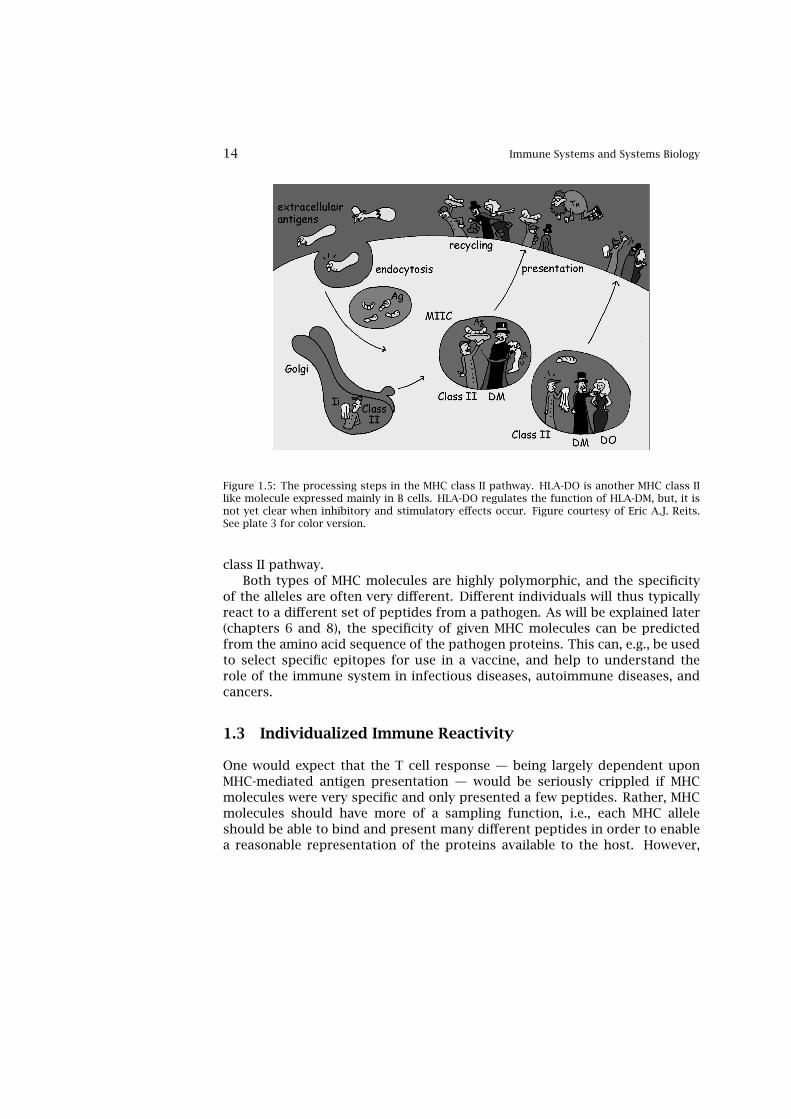
14 Immune Systems and Systems Biology
Figure 1.5: The processing steps in the MHC class II pathway. HLA-DO is another MHC class IIlike molecule expressed mainly in B cells. HLA-DO regulates the function of HLA-DM, but, it isnot yet clear when inhibitory and stimulatory effects occur. Figure courtesy of Eric A.J. Reits.See plate 3 for color version.
class II pathway.Both types of MHC molecules are highly polymorphic, and the specificity
of the alleles are often very different. Different individuals will thus typicallyreact to a different set of peptides from a pathogen. As will be explained later(chapters 6 and 8), the specificity of given MHC molecules can be predictedfrom the amino acid sequence of the pathogen proteins. This can, e.g., be usedto select specific epitopes for use in a vaccine, and help to understand therole of the immune system in infectious diseases, autoimmune diseases, andcancers.
1.3 Individualized Immune Reactivity
One would expect that the T cell response — being largely dependent uponMHC-mediated antigen presentation — would be seriously crippled if MHCmolecules were very specific and only presented a few peptides. Rather, MHCmolecules should have more of a sampling function, i.e., each MHC alleleshould be able to bind and present many different peptides in order to enablea reasonable representation of the proteins available to the host. However,

Individualized Immune Reactivity 15
any sampling function involves some kind of specificity and any degree ofspecificity has a flip side; those epitopes which are ignored by the MHC wouldconstitute immunological "blind spots." From the point of view of the invader,such blind spots would amount to a constant evolutionary pressure to removeMHC presentable epitopes.
This evolutionary pressure would be persistent and unchanging if therewere one, and only one, MHC specificity within the species; and pathogenswould eventually succeed in escaping immune control. The immune systemhas solved this potential problem through MHC polymorphism. In fact, asmentioned above, the MHC is the most polymorphic gene system known. Ona population basis, hundreds of alleles have been found for most of the MHCencoding loci (see figure 12.1 for the number of MHC sequences identifieduntil recently). On an individual basis, only one (homozygous) or two (het-erozygous) of these alleles are expressed per locus. The number of MHC lociper individual also differs among species. While a heterozygous human wouldhave six MHC class I genes (coded in three loci), e.g., the rhesus macaque canhave as many as 22 active MHC class I genes [Daza-Vamenta et al., 2004]. Thepolymorphism affects the peptide binding specificity of the MHC; one allelicMHC product will recognize one part of the universe of peptides, whereas an-other allelic MHC product will recognize a different part of this universe. Thisleads to an individualized immune reactivity. No two individuals will have thesame set of immunological "blind spots" and no microorganism could there-fore evolve to easily circumvent the immune systems of the entire species.Thus, polymorphism is what allows the MHC to exercise some degree of speci-ficity. From a practical point of view, MHC polymorphism is a huge challengeto any T cell epitope discovery process, underpinning the need for bioinfor-matical analysis and resources.


Chapter 2
Contemporary Challenges tothe Immune System
2.1 Infectious Diseases in the New Millennium
More than 400 microbial agents are associated with disease in healthy adulthumans [RAC, 2002]. The number of agents known to be a threat to humanand animal health is large and it may not be not feasible (or possible) to de-velop in a cost-effective manner conventional vaccines against all emergingpathogens: there are only licensed vaccines in the United states for 22 mi-crobial agents [FDA, 2003]. Moreover, since it will take a very long time toestimate the true virulence of these pathogens, the use of complete or partialorganisms might not be safe. Immunological bioinformatics can make an im-portant contribution to the rapid design of novel vaccines by identifying themost immunogenic regions on the pathogens. These regions can subsequentlybe used as candidates for a rational vaccine design.
2.2 Major Killers in the World
It is estimated that 11 million (19%) of the 57 million people who died in theworld in 2002 were killed by infectious or parasitic infection [WHO, 2004a].Table 2.1 shows the major causes of death in the world from infectious dis-eases.
The three main single infectious diseases are HIV/AIDS, tuberculosis, andMalaria, each of which causes more than 1 million deaths.
17

18 Contemporary Challenges to the Immune System
2.2.1 AIDS
Acquired immunodeficiency syndrome (AIDS), which is caused by the humanimmunodeficiency virus (HIV), is now the leading cause of death in youngadults worldwide. WHO states that tackling HIV/AIDS is the world’s most ur-gent public health challenge [WHO, 2004b]. More than 20 million people havedied from AIDS and an estimated 34 to 46 million others are now infected withthe virus. There is as yet no vaccine and no definite cure.
HIV is an enveloped retrovirus that replicates in cells of the immune sys-tem. HIV belongs to a group of retroviruses called the lentiviruses[Lever, 2000].These viruses cause diseases that progress gradually. Often lentivurses per-sist after an infection and continue to replicate for many years before causingovert signs of disease. HIV-1 and HIV-2 are the only known human lentiviruses.
HIV uses the CD4 protein (often expressed by helper T cells andmacrophages) and a chemokine receptor (CCR5 or CXCR4) to infect cells[Pierson and Doms, 2003]. The viral replication occurs only in activated Tcells. Primary infection of humans with HIV-1 is associated with an acutemononucleosis-like clinical syndrome which appears approximately 36 weeksfollowing infection [Hansasuta and Rowland-Jones, 2001]. Initially, the con-centration of virus in the blood (viremia) can be high, but rapidly diminishesas cytotoxic T cell responses develop. Despite the ongoing immune responseHIV infection is not eliminated: HIV establishes a state of persistent infectionin which the virus is continually replicating in newly infected cells. The mainreason that the infection is not cleared is that HIV can easily generate immuneescape mutants: it has a rapid replication rate and a fast mutation rate, whichlead to the generation of many variants of HIV in a single infected patient inthe course of one day.
The main effect of HIV on the immune system is the loss of CD4+ T cells(for a review see, e.g., Hazenberg et al. [2000]). There are at least two dom-inant mechanisms for this. First, direct viral killing of infected T cells; andsecond, killing of infected T cells by cytotoxic lymphocytes that recognize vi-ral peptides. The currently used HAART (highly active antiretroviral therapy )treatment consists of combinations of viral protease inhibitors together withnucleoside analogues and causes a rapid decrease in virus levels and a slowerincrease in CD4+ T cell counts [Berger et al., 1998]. The treatment usually hassevere sideeffects, and many patients cannot continue the treatment for longperiods [Laurence, 2004]. Moreover, in the developing world, where HIV/AIDShas its largest burden, HAART is too expensive for use in every HIV-infected in-dividual. Without treatment the concentration of CD4+ T cells (the CD+ count)decreases gradually, and the body becomes progressively more susceptible toopportunistic infections. Eventually, most HIV-infected individuals developAIDS and die; however a small minority remain healthy for many years, with

Major Killers in the World 19
no apparent ill effects of infection. Hopefully, we will be able to learn fromthese long term nonprogressors how HIV infection can be controlled. If so,it will be possible one day to develop effective vaccines and therapies againstHIV.
2.2.2 Tuberculosis
Tuberculosis (TB) is another emerging public health threat. The Mycobac-terium tuberculosis bacteria (Mtb), the causative agent of TB, is spread fromperson to person by airborne droplets expelled from the lungs when a per-son with TB coughs, sneezes, or speaks. Outbreaks may therefore occur inclosed settings and under crowded living conditions such as homeless shel-ters and prisons. It is estimated that onethird of the world’s population (1.86billion people) is infected with Mtb, and 16.2 million people have TB. Approx-imately 10% of those infected with Mtb develop TB later in life, most of thema few years after infection. Mtb-infected persons can also develop TB if theirimmune system is impaired, e.g., by HIV infection. In 1995, the year withthe highest TB casualty rate to date, nearly 3 million people died worldwidefrom the disease. Currently, there is only one licensed vaccine against TB inthe United States but it is not recommended for use. This vaccine, bacilleCalmette-Guérin (BCG), is reportedly highly variable in its efficacy to preventadult pulmonary TB. It may have a lower efficiency in poor tropical societieswhere people are more exposed to other mycobacteria in the environment.The protection offered by the vaccine normally lasts until adolescence. TheJordan report, NIAID, 2000 states that "For many reasons, the development ofimproved anti-TB vaccines has become a necessity for adequate control andelimination of tuberculosis. These reasons include the spread of (multidrugresistant) MDR-TB, the global burden of the TB epidemic, the growing TB/HIVcoepidemic in large areas of the world, the enormous practical barriers to con-trolling TB adequately through administration of what are complicated andcostly treatment regimens, inadequate diagnostic methods, and the relativeineffectiveness of the current BCG vaccines."
2.2.3 Malaria
Malaria is a serious and sometimes fatal disease caused by a parasite. Patientswith malaria typically become very sick with high fevers, shaking chills, andflulike illness. Four kinds of malaria parasites can infect humans: Plasmodiumfalciparum, P. vivax, P. ovale, and P. malariae. Infection with any of the malariaspecies can make a person feel very ill, but infection with P. falciparum, if notpromptly treated, may be fatal. Although malaria can be a fatal disease, illness

20 Contemporary Challenges to the Immune System
and death from malaria are largely preventable. The World Health Organi-zation estimates that each year 300 to 500 million cases of malaria occur andthat more than 1 million people die of malaria, most of them in young children.Since many countries with malaria are already among the poorer nations, thedisease maintains a vicious cycle of disease and poverty. Malaria has beeneradicated from many developed countries with temperate climates. However,the disease remains a major health problem in many developing countries,in tropical and subtropical parts of the world. An eradication campaign wasstarted in the 1950s, but it failed due to problems, including the resistance ofmosquitoes to insecticides used to kill them, the resistance of malaria para-sites to drugs used to treat them, and administrative issues. In addition, theeradication campaign never involved most of Africa, where malaria is mostcommon.
Usually, people get malaria by being bitten by an infected female Anophe-les mosquito. Only Anopheles mosquitoes can transmit malaria and they musthave been infected by a previous blood meal taken from an infected per-son. When a mosquito bites, a small amount of blood is taken which con-tains the microscopic malaria parasites. The parasites grow and mature inthe mosquito’s gut for a week or more, then travel to the mosquito’s salivaryglands. When the mosquito next takes a blood meal, these parasites mix withthe saliva and are injected into the bite. Once in the blood, the parasites travelto the liver and enter liver cells to grow and multiply. During this incubationperiod, the infected person has no symptoms. After as little as 8 days or aslong as several months, the parasites leave the liver cells and enter red bloodcells. Once in the cells, they continue to grow and multiply. After they mature,the infected red blood cells rupture, freeing the parasites to attack and enterother red blood cells. Toxins released when the red cells burst are what causethe typical fever, chills, and flulike malaria symptoms. If a mosquito bites thisinfected person and ingests certain types of malaria parasites (gametocytes),the cycle of transmission continues.
Because the malaria parasite is found in red blood cells, malaria can alsobe transmitted through blood transfusion, organ transplant, or the shareduse of needles or syringes contaminated with blood. Malaria may also betransmitted from a mother to her fetus before or during delivery (congen-ital malaria) (This discussion has about malaria has been adopted fromhttp://www.cdc.gov/malaria/faq.htm).
2.3 Childhood Diseases
The term childhood diseases normally covers mumps, measles, rubella, chick-enpox, whooping cough, smallpox, diphtheria, tetanus, and polio [DMID,

Childhood Diseases 21
2004]. These diseases have successfully been controlled in the developedworld through vaccines. Over 1 million still die each year from childhooddiseases for which vaccines are available. This is mainly due to the vaccinesnot being available in many underdeveloped countries, and in Russia and theformer East Bloc countries where the healthcare systems have deterioratedover the last 15 years.
Even in the developed world challenges still exist [DMID, 2004]:
• Elimination of adverse side effects of vaccines
• Control of childhood diseases in immunologically compromised children
• Development of more easily administered, "child-friendly" vaccines
• Better control of persisting childhood disease threats such as infectionscaused by rapidly evolving organisms like streptococcus and many mi-crobes causing pneumococcal infection
2.3.1 Respiratory Infections
Infections of the respiratory tract continue to be the leading cause of acuteillness worldwide. Upper respiratory infections (URIs) such as the commoncold, strep throat, sinusitis, and otitis media (ear infections) are very common,especially in children, but seldom have serious or life-threatening complica-tions. Lower respiratory infections (LRIs) include more serious illnesses suchas influenza, bronchitis, pertussis (whooping cough), pneumonia, and tuber-culosis and are the leading contributors to the more than 4 million deathscaused each year by respiratory infections [NIAID, 2002b]. The most commonetiological agents of pneumonia are Streptococcus pneumoniae, Haemophilusinfluenzae, and respiratory syncytial virus (RSV) [NIAID, 2002b]. In one studyRSV was detected in 36.3% and adenoviruses in 14.3% of cases of acute LRIs[Videla et al., 1998].
2.3.2 Diarrheal Diseases
Another major cause of death is diarrheal diseases which may be caused by anumber of pathogens. Even when the most sophisticated methods and diag-nostic reagents are used, more than half of the cases of diarrheal illness can-not be ascribed to a particular agent. Important pathogens include cholera,Shiga toxin–producing Escherichia coli (STEC), enteropathogenic E. coli (EPEC),enterotoxigenic E. coli (ETEC), Helicobacter pylori, rotavirus, caliciviruses [Jianget al., 2000], Shigella, Salmonella typhi, and Campylobacter [NIAID, 2002b].
22 Contemporary Challenges to the Immune System
Typhoid fever, which is caused by Salmonella typhi, remains a serious pub-lic health problem throughout the world, with an estimated 16 to 33 millioncases and 500,000 deaths annually [NIAID, 2002b].
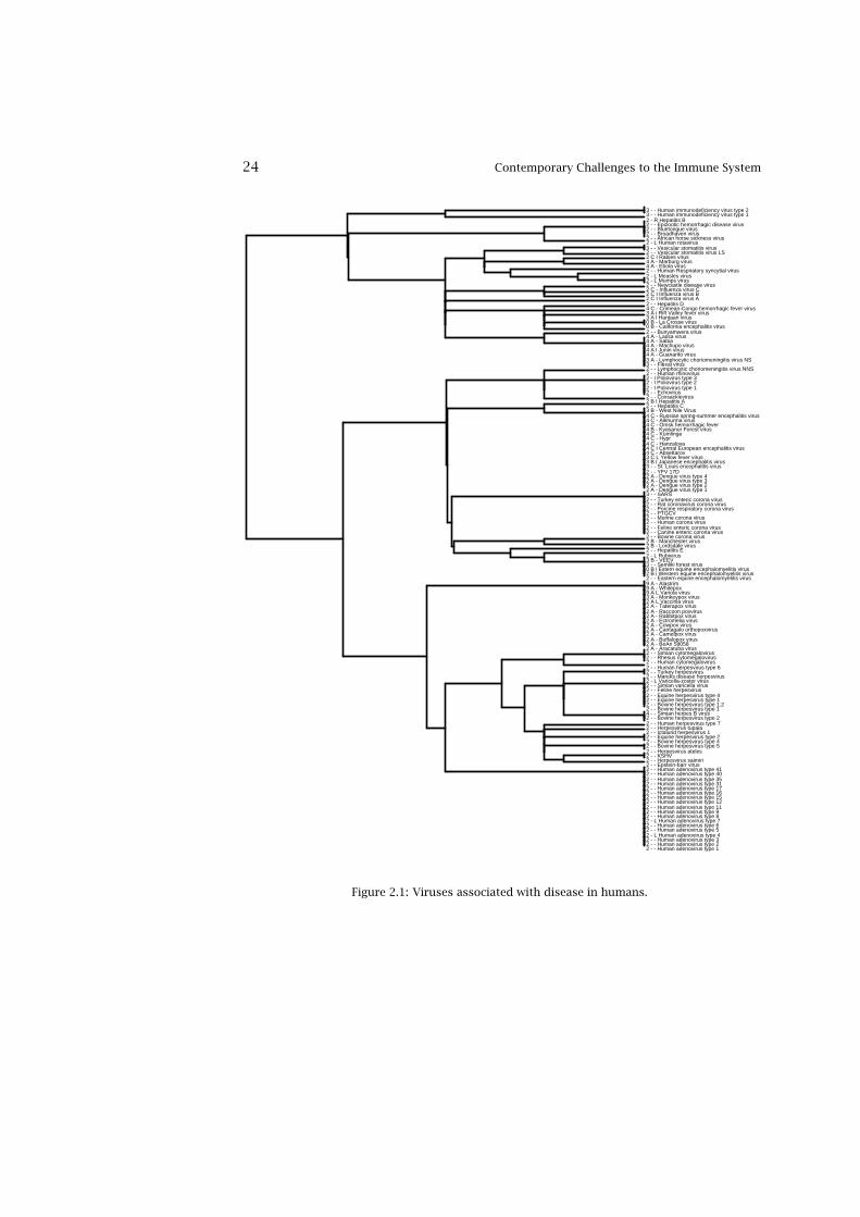
2.4 Clustering of Infectious Disease Organisms
It is difficult to get an overview of the different human pathogens (microorgan-isms associated with diseases in humans). Figures 2.1 through 2.4 shows theviruses, bacteria, parasites, and fungi associated with diseases in humans. Theclustering is based on the number of terms in the Swiss-Prot family descriptionthat are identical between the two organisms. The data were extracted fromhttp://www.cbs.dtu.dk/databases/Dodo.
The pathogens have been selected from appendix B of the RecombinantDNA Advisory Committee guidelines [RAC, 2002] which includes those biolog-ical agents known to infect humans, as well as selected animal agents that maypose theoretical risks if inoculated into humans. RAC divides pathogens intofour classes.
1. Risk group 1 (RG1). Agents that are not associated with disease inhealthy adult humans
2. Risk group 2 (RG2). Agents that are associated with human diseasewhich is rarely serious and for which preventive or therapeutic inter-ventions are often available
3. Risk group 3 (RG3). Agents that are associated with serious or lethalhuman disease for which preventive or therapeutic interventions may beavailable (high individual risk but low community risk)
4. Risk group 4 (RG4). Agents that are likely to cause serious or lethalhuman disease for which preventive or therapeutic interventions are notusually available (high individual risk and high community risk)
In figures 2.1–2.4 names for human pathogens are shown for viruses, bac-teria, parasites and fungi. The first column before the pathogen name is theRAC classification, the second column is the classification of the pathogensaccording to the Centers for Disease Control and Prevention (CDC) bioterrorcategories A–C, where category A pathogens are considered the worst bioterrorthreats [CDC, 2003].
The third column before the pathogen name contains a dash if no vaccineis available for the pathogen and a letter indicating the type of vaccine if one isavailable (A: acellular/adsorbet; C: conjugate; I: inactivated; L: live; P: polysac-charide; R: recombinant; S staphage lysate; T: toxoid). Lower case indicatesthat the vaccine is released as an investigational new drug (IND)).

Clustering of Infectious Disease Organisms 23
Cause Deaths (1000) Percent of total deathsInfectious and parasitic diseases 10,904 19.1Tuberculosis 1,566 2.7STIs excluding HIV 180 0.3
Syphilis 157 0.3Chlamydia 9 0.0Gonorrhea 1 0.0
HIV/AIDS 2,777 4.9Diarrheal diseases 1,798 3.2Childhood diseases 1,124 2.0
Pertussis 294 0.5Poliomyelitis 1 0.0Diphtheria 5 0.0Measles 611 1.1Tetanus 214 0.4
Meningitis 173 0.3Hepatitis B 103 0.2Hepatitis C 54 0.1Malaria 1,272 2.2Tropical diseases 129 0.2
Trypanosomiasis 48 0.1Chagas’ disease 14 0.0Schistosomiasis 15 0.0Leishmaniasis 51 0.1Lymphatic filariasis 0 0.0Onchocerciasis 0 0.0
Leprosy 6 0.0Dengue 19 0.0Japanese encephalitis 14 0.0Trachoma 0 0.0Intestinal nematode infections 12 0.0
Ascariasis 3 0.0Trichuriasis 3 0.0Hookworm disease 3 0.0
Respiratory infections 3,963 6.9Lower respiratory infections 3,884 6.8Upper respiratory infections 75 0.1
Otitis media 4 0.0
Table 2.1: Major causes of death in the world from infectious diseases (2002). The table hasbeen adapted from [WHO, 2004a]. STIs: Sexually transmitted Infections.
24 Contemporary Challenges to the Immune System
2 - - Human adenovirus type 12 - - Human adenovirus type 22 - - Human adenovirus type 32 - L Human adenovirus type 42 - - Human adenovirus type 52 - - Human adenovirus type 62 - L Human adenovirus type 72 - - Human adenovirus type 82 - - Human adenovirus type 92 - - Human adenovirus type 112 - - Human adenovirus type 122 - - Human adenovirus type 152 - - Human adenovirus type 162 - - Human adenovirus type 172 - - Human adenovirus type 312 - - Human adenovirus type 352 - - Human adenovirus type 402 - - Human adenovirus type 412 - - Epstein-barr virus2 - - Herpesvirus saimiri2 - - KSHV2 - - Herpesvirus ateles2 - - Bovine herpesvirus type 52 - - Bovine herpesvirus type 42 - - Equine herpesvirus type 22 - - Ictalurid herpesvirus 12 - - Herpesvirus tupaia2 - - Human herpesvirus type 72 - - Bovine herpesvirus type 24 - - Simian herpes B virus2 - - Bovine herpesvirus type 12 - - Bovine herpesvirus type 1.22 - - Equine herpesvirus type 12 - - Equine herpesvirus type 42 - - Feline herpesvirus2 - - Simian varicella virus2 - L Varicella-zoster virus2 - - Mareks disease herpesvirus2 - - Turkey herpesvirus2 - - Human herpesvirus type 62 - - Human cytomegalovirus2 - - Rhesus cytomegalovirus2 - - Simian cytomegalovirus2 A - Aracatuba virus2 A - BeAn 580582 A - Buffalopox virus2 A - Camelpox virus2 A - Cantagalo orthopoxvirus2 A - Cowpox virus2 A - Ectromelia virus2 A - Rabbitpox virus2 A - Raccoon poxvirus2 A - Taterapox virus2 A L Vaccinia virus3 A - Monkeypox virus9 A L Variola virus9 A - Whitepox9 A - Alastrim2 - - Eastern equine encephalomyelitis virus2 B i Western equine encephalomyelitis virus0 B i Estern equine encephalomyelitis virus3 - - Semliki forest virus3 B - VEEV2 - L Rubivirus2 - - Hepatitis E2 B - Lordsdale virus2 B - Manchester virus2 - - Bovine corona virus2 - - Canine enteric corona virus2 - - Feline enteric corona virus2 - - Human corona virus2 - - Murine corona virus2 - - PTGCV2 - - Porcine respiratory corona virus2 - - Rat coronavirus corona virus2 - - Turkey enteric corona virus3 - - SARS2 A - Dengue virus type 12 A - Dengue virus type 22 A - Dengue virus type 32 A - Dengue virus type 42 - - YFV 17D3 - - St. Louis encephalitis virus3 B I Japanese encephalitis virus3 C L Yellow fever virus4 C - Absettarov4 C I Central European encephalitis virus4 C - Hanzalova4 C - Hypr4 C - Kumlinge4 B - Kyasanur Forest virus4 C - Omsk hemorrhagic fever4 C - Alkhurma virus4 C - Russian spring-summer encephalitis virus3 B - West Nile Virus2 - - Hepatitis C2 B I Hepatitis A2 - - Coxsackievirus2 - - Echovirus2 - I Poliovirus type 12 - I Poliovirus type 22 - I Poliovirus type 32 - - Human rhinovirus2 - - Lymphocytic choriomeningitis virus NNS3 - - Flexal virus3 A - Lymphocytic choriomeningitis virus NS4 A - Guanarito virus4 A l Junin virus4 A - Machupo virus4 A - Sabia4 A - Lassa virus2 - - Bunyamwera virus0 B - California encephalitis virus0 B - La Crosse virus3 A l Hantaan virus3 A i Rift Valley fever virus4 C - Crimean-Congo hemorrhagic fever virus2 - - Hepatitis D2 C I Influenza virus A2 C I Influenza virus B2 C - Influenza virus C2 - - Newcastle disease virus2 - L Mumps virus2 - L Measles virus2 - - Human Respiratory syncytial virus4 A - Ebola virus4 A - Marburg virus2 C I Rabies virus2 - - Vesicular stomatitis virus LS3 - - Vesicular stomatitis virus2 - L Human rotavirus2 - - African horse sickness virus2 - - Broadhaven virus2 - - Bluetongue virus2 - - Epizootic hemorrhagic disease virus2 - R Hepatitis B3 - - Human immunodeficiency virus type 13 - - Human immunodeficiency virus type 2
Figure 2.1: Viruses associated with disease in humans.

Clustering of Infectious Disease Organisms 25
2 - - Acinetobacter baumannii2 - - Moraxella bovis2 - - Moraxella catarrhalis2 - - Moraxella lacunata2 - - Moraxella nonliquefaciens2 - - Moraxella sp2 - - Aeromonas hydrophila2 - - Legionella pneumophila3 B i Coxiella burnetii3 A l Francisella tularensis2 - - Actinobacillus actinomycetemcomitans2 - - Actinobacillus pleuropneumoniae2 - - Actinobacillus suis2 - - Haemophilus ducreyi2 - C Haemophilus influenzae3 - - Pasteurella multocida2 - - Edwardsiella tarda2 B - Salmonella enterica2 B - Salmonella enteritidis2 B - Salmonella gallinarum2 B - Salmonella meleagridis2 B - Salmonella paratyphi2 B - Salmonella pullorum2 B l Salmonella typhi2 B - Salmonella typhimurium2 - - Klebsiella aerogenes2 - - Klebsiella pneumoniae2 - - Klebsiella pneumoniae ozaenae2 - - Klebsiella sp2 B - Yersinia enterocolitica3 A I Yersinia pestis2 B I Escherichia coli 01112 B - Escherichia coli 01272 B - Escherichia coli 01572 B - Shigella boydii2 - - Klebsiella ornithinolytica2 - - Klebsiella planticola2 - - Klebsiella terrigena2 B - Shigella dysenteriae2 B - Shigella flexneri2 B - Shigella sonnei2 B I Vibrio cholerae2 B - Vibrio parahaemolyticus2 B - Vibrio vulnificus2 - - Campylobacter coli2 - - Campylobacter fetus2 B - Campylobacter jejuni2 - - Helicobacter pylori2 - - Helicobacter pylori J992 - - Bartonella henselae2 - - Bartonella quintana2 - - Bartonella vinsonii2 - - Bartonella vinsonii berkhofii3 - - Bartonella bacilliformis3 - - Bartonella clarridgeiae3 - - Bartonella doshiae3 - - Bartonella elizabethae3 - - Bartonella taylorii3 B - Brucella abortus3 B - Brucella canis3 B - Brucella suis3 C - Rickettsia akari3 C - Rickettsia australis3 C - Rickettsia canada3 C - Rickettsia conorii3 B I Rickettsia prowazekii3 C I Rickettsia rickettsii3 C - Rickettsia sibirica3 C - Rickettsia typhi3 C - Rickettsia tsutsugamushi2 - A Bordetella pertussis2 - - Burkholderia cepacia2 - - Burkholderia sp2 - - Burkholderia sp RASC2 - - Burkholderia thailandensis2 - - Burkholderia vietnamiensis2 - - Burkholderia glumae2 - - Burkholderia pyrrocinia3 B - Burkholderia mallei3 B - Burkholderia pseudomallei2 - - Burkholderia eutrophus2 - - Burkholderia pickettii2 - - Neisseria gonorrhoeae2 - P Neisseria meningitidis2 - P Neisseria meningitidis A2 - - Neisseria meningitidis B2 - P Neisseria meningitidis C2 B - Salmonella arizonae2 - R Borrelia burgdorferi2 - - Treponema pallidum2 - - Treponema pallidum pertenue2 - - Leptospira interrogans2 - - Chlamydia psittaci2 - - Chlamydia pneumoniae2 - - Chlamydia trachomatis2 - - Arcanobacterium haemolyticum2 - T Corynebacterium diphtheriae2 - - Corynebacterium pseudotuberculosis2 - - Mycobacterium avium complex2 - - Mycobacterium asiaticum2 - - Mycobacterium chelonae2 - - Mycobacterium fortuitum2 - - Mycobacterium kansasii2 - - Mycobacterium leprae2 - - Mycobacterium malmoense2 - - Mycobacterium marinum2 - - Mycobacterium paratuberculosis2 - - Mycobacterium scrofulaceum2 - - Mycobacterium szulgai2 - - Mycobacterium ulcerans2 - - Mycobacterium xenopi3 - - Mycobacterium bovis3 C L Mycobacterium tuberculosis2 - - Nocardia asteroides2 - - Rhodococcus equi2 A A Bacillus anthracis2 B - Brochothrix thermosphacta2 B - Listeria grayi2 B - Listeria innocua2 B - Listeria ivanovii2 B - Listeria monocytogenes2 B - Listeria seeligeri2 B - Listeria welshimeri2 - S Staphylococcus aureus2 - S Staphylococcus aureus Mu502 - S Staphylococcus aureus N3152 - S Staphylococcus aureus MW22 A - Clostridium botulinum2 - - Clostridium histolyticum2 - - Clostridium septicum2 - T Clostridium tetani2 - P Streptococcus pneumoniae2 - - Streptococcus pyogenes2 - - Streptococcus pyogenes M52 - - Streptococcus pyogenes M182 - - Erysipelothrix rhusiopathiae2 - - Arcanobacterium pyogenes2 - - Amycolata autotrophica2 - - Clostridium novyi
Figure 2.2: Bacteria associated with disease in humans.

26 Contemporary Challenges to the Immune System
2 - - Ascaris lumbricoides suum2 - - Toxocara canis2 - - Brugia malayi2 - - Onchocerca volvulus2 - - Trichinella spiralis2 - - Echinococcus granulosus2 - - Echinococcus multilocularis2 - - Taenia solium2 - - Fasciola hepatica2 - - Schistosoma haematobium2 - - Schistosoma japonicum2 - - Schistosoma mansoni2 B - Entamoeba histolytica2 - - Leishmania braziliensis2 - - Leishmania donovani2 - - Leishmania major2 - - Leishmania mexicana2 - - Leishmania peruviana2 - - Trypanosoma brucei brucei2 - - Trypanosoma brucei rhodesiense2 - - Trypanosoma brucei gambiense2 - - Trypanosoma brucei congolense2 - - Trypanosoma brucei cruzi2 - - Trypanosoma brucei equiperdum2 - - Trypanosoma brucei lewisi2 - - Trypanosoma brucei rangeli2 - - Trypanosoma brucei vivax0 B - Encephalitozoon cuniculi2 B - Microsporidium africanum2 B - Microsporidium ceylonensis0 B - Enterocytozoon bieneusi0 B - Vittaforma corneae0 B - Brachiola vesicularum0 B - Brachiola connori0 B - Encephalitozoon intestinalis0 B - Encephalitozoon hellem0 B - Nosema ocularum0 B - Nosema algerae0 B - Pleistophora sp.0 B - Trachipleistophora hominis0 B - Trachipleistophora anthropophthera2 B - Giardia lamblia2 - - Naegleria fowleri2 B - Cyclospora cayatanensis2 - - Eimeria acervulina2 - - Eimeria bovis2 - - Eimeria tenella2 - - Neospora2 - - Sarcocystis muris2 B - Toxoplasma gondii2 B - Cryptosporidium parvum2 - - Plasmodium cynomolgi2 - - Plasmodium falciparum2 - - Plasmodium malariae2 - - Plasmodium vivax
Figure 2.3: Parasites associated with disease in humans.

Clustering of Infectious Disease Organisms 27
2 - - Ajellomyces dermatitidis
3 - - Ajellomyces capsulata
2 - - Trichophyton rubrum
2 - - Trichophyton tonsurans
3 - - Coccidioides immitis
2 - - Exophiala dermatitidis
2 - - Sporothrix schenckii
2 - - Cryptococcus neoformans
2 - - Microsporum
Figure 2.4: Fungi associated with disease in humans.
28 Contemporary Challenges to the Immune System
2.5 Biodefense Targets
Vaccines have only been made for 14 of the more than 123 agents on the NI-AID A–C list. For many of the bacterial agents antibiotic treatment is possible,but may be inefficient if the agent is inhaled [NIAID, 2002a]. The CDC hasdefined three categories A–C, where category A pathogens are considered tobe the worst bioterror threats [CDC, 2003]. Category A agents include Bacil-lus anthracis (anthrax), Clostridium botulinum toxin (botulism), Yersinia pestis(plague) Variola major (smallpox), Francisella tularensis (tularemia) and viralhemorrhagic fevers.
Anthrax Even with antibiotic treatment inhalation anthrax is a potentially fa-tal (40-75% fatality) disease [NIAID, 2002a]. An anthrax vaccine adsorbed(AVA) is licensed in the United States [FDA, 2003]. There are no datato support the efficacy of AVA for pulmonary anthrax in humans, but ithas been established that the protective antigen (PA) of B. anthracis in-duces significant protective immunity against inhalation spore challengein animal models and that PA is the component of AVA responsible forgenerating such immunity [NIAID, 2000]. Pilot lots of a recombinant PAvaccine are currently being produced [NIAID, 2002a]. The 3D structureof the anthrax toxin has recently been determined. This may be used todiscover vaccines or compounds that block the effect of the toxin.
Smallpox Smallpox was eradicated in 1977. The mortality from smallpoxinfections is approximately 30% [NIAID, 2002a]. The vaccine has se-rious side effects and is associated with complications which may belife-threatening, especially in persons with an impaired immune system[NIAID, 2002a]. Development of a safer vaccine is therefore a priority.A modified vaccinia Ankara (MVA) vaccine for evaluation in a phase Iclinical study is being produced [NIAID, 2002a].
Plague Natural epidemics of plague have been primarily bubonic plague (char-acterized by enlarged lymph nodes ("swollen glands") that are tender andpainful), which is transmitted by fleas from infected rodents. Inhala-tion of aerosolized bacilli can lead to a pneumonic plague (a form ofplague that can spread through the air from person to person; character-ized by lung involvement) which untreated has a mortality rate that ap-proaches 100%. Aggressive antibiotic treatment can be effective [NIAID,2003] No vaccine is currently licensed in the United States. A formalin-killed, whole-cell vaccine (USP) was available until 1999. It could preventbubonic plague but could not prevent pneumonic plague [NIAID, 2003].Phase I human trials are planned for candidate vaccines based on the twoantigens F1 and V [NIAID, 2003].
Biodefense Targets 29
Botulism Botulinum toxin is the etiologic agent responsible for the diseasebotulism, which is characterized by peripheral neuromuscular blockade.Seven antigenic types (A-G) of the toxin exist. All seven toxins causesimilar clinical presentation and disease; botulinum toxins A, B, and Eare responsible for the vast majority of foodborne botulism cases in theUnited States. The heavy chain is not toxic, and has been shown to evokecomplete protection against the toxin. Sequencing of the C. botulinumHall strain A bacterium genome has been completed.
Tularemia Francisella tularensis, which causes tularemia, is a non–spore-forming, facultative intracellular bacterium. If untreated, the diseasecould lead to respiratory failure. Treatment with antibiotics reducesmortality for naturally acquired cases by 2 to 60%. A live attenuatedtularemia vaccine developed by the Department of Defense (DoD) hasbeen administered under an investigational new drug (IND) applicationto thousands of volunteers [NIAID, 2003]. In vivo studies demonstratethat either CD4 or CD8 T cells can mediate resolution of live vaccinestrain (LVS) infections. Antibodies appear to contribute little, if anything,to protective immunity [NIAID, 2002a].
Viral hemorrhagic fevers (VHFs) Viral hemorrhagic fevers encompass agroup of similar diseases caused by four types of viruses:
Arenaviruses, associated with Argentine, Bolivian, and Venezuelan hem-orrhagic fevers, Lassa fever, and Sabia virus–associated hemorrhagicfever
Bunyaviruses, including Crimean-Congo hemorrhagic fever, Rift Valleyfever, and Hantavirus infection
Filoviruses, comprising Ebola and Marburg hemorrhagic fevers
Hemorrhagic flaviviruses, including yellow fever, dengue hemorrhagicfever, West Nile virus, Kyasanur Forest disease, and Omsk hemor-rhagic fever.
With very few exceptions (yellow fever), no vaccines or proven treatmentsexist, and many of the diseases are highly fatal. For Ebola hemorrhagicfever, immunization with an adenoviral (ADV) vector encoding the Ebolaglycoprotein (GP) has been shown to protect against disease in cynomol-gus macaques. Two tetravalent dengue vaccines will be studied in non-human primates in 2003 [NIAID, 2003], and work has been initiated onMarburg and West Nile virus vaccines [NIAID, 2003].
30 Contemporary Challenges to the Immune System
2.6 Cancer
Cancer is one of the three leading causes of death in industrialized countries.Cancers are caused by cells which grow progressively without any regulation.Thus, curing cancer requires destruction of these cells. A possible way ofachieving this would be to generate an immune response against these cells(see for a review, e.g., Crittenden et al. [2005]). This implies that the immunesystem should be able to discriminate tumor cells from healthy cells. Theantigenic differentiation in a tumor cell can provide such discriminatory sig-nals. For example, proteins that are crucial in cell cycle regulation, like p53,are going through differentiation in tumor cells. If the differentiated parts ofthese proteins are presented to T cells on MHC molecules, a T cell responseagainst tumors might be invoked [Marincola et al., 2003, Mocellin et al., 2004].These tumor rejection antigens are usually tumor specific, although they canbe shared by tumors of a similar origin. This makes the identification of tu-mor antigens a very time-consuming process, because for every cancer typenew tumor antigens need to be identified.
For over a century researchers have been trying to invoke antitumor im-mune responses, but, there is still no successful treatment based on immuneresponses, except for a few types of cancer (see e.g., de Leo [2005]). The mainreason is that tumors can escape an immune response in many ways [Maparaand Sykes, 2004]. Tumors are generally genetically unstable, and they canlose their antigens by mutation. Moreover, some tumors lose expression of aparticular MHC molecule, totally blocking antigen presentation. These tumorsmay become susceptible to a natural killer (NK) cell–mediated response Wuand Lanier [2003], but, tumors that lose only one or two MHC molecules mayavoid recognition by NK cells.
Recent developments in understanding antigen presentation and themolecules involved in T cell activation together with fast identification of tu-mor epitopes by bioinformatics tools might allow for new immunotherapeuticstrategies.
2.7 Allergy
Allergy belongs to the class of immune responses called hypersensitivity re-actions. These are harmful immune responses that produce tissue injury andmay cause serious disease. Genetic factors contribute to the development ofallergy, but environmental factors may also be important. Allergic reactionsare caused by a special class of antibodies called immunoglobulin E (IgE) an-tibodies [Janeway et al., 2001]. IgE responses are, under normal physiologicalconditions protective, especially in response to parasitic worms, which are

Autoimmune Diseases 31
prevalent in less developed countries [Hagel et al., 2004]. In the industrial-ized countries, however, due to higher standards of hygienic conditions, IgEresponses occur almost entirely against allergens. Almost half of the inhab-itants of North America and Europe have allergies to one or more commonenvironmental antigens. These allergies are rarely life-threatening, but, theycause much distress and lost time during everyday life.
Allergic reactions occur when allergens cross-link preexisting IgE bound tothe mast cells [Gould et al., 2003]. Mast cells line the body surfaces and arevery important in signaling local infections to other parts of the immune sys-tem. Once activated, they induce inflammatory reactions by secreting severalchemical mediators stored in performed vesicles. In allergy, these reactionscan cause symptoms that range from itching and burning of the skin to life-threatening systemic anaphylaxis. The severity of the symptoms depends onthe dose of antigen and its route of entry. The immediate allergic reactioncaused by mast cells is followed by a more sustained inflammation: the late-phase response. This late response involves the recruitment of other effec-tor cells, especially T helper type 2 lymphocytes, eosinophils, and basophils,which contribute significantly to the immunopathology of an allergic response.
For allergies that are not very severe, the best therapy is avoidance of theallergen. This not only avoids the symptoms but also decreases with time theamount of specific IgE in the blood, the main cause of the allergic reactions.Except for avoidance and the use of drugs to treat the symptoms of allergicdisease and limit the inflammatory response, two treatments are commonlyused in clinical practice [Stokes and Casale, 2004]. The first one is desensi-tization where the aim is to shift the antibody response from IgE to IgG. IgGantibodies can bind to the allergen and thus prevent it from causing allergicreactions. Patients are injected with escalating doses of allergen, starting withtiny amounts. This injection schedule gradually diverts the IgE-dominated re-sponse, driven by T helper 2 cells, to one driven by T helper 1 cells, with theconsequent downregulation of IgE production. A potential complication ofthe desensitization approach is the risk of inducing IgE-mediated allergic re-sponses. The second treatment consists of blocking of the effector pathways,like disabling the recruitment of eosinophils to sites of allergic inflammation.This can be done by using specific migration molecules that all immune cellshave. Finally, a new promise in curing allergy is the use of peptide-based vac-cines [Alexander et al., 2002].
2.8 Autoimmune Diseases
One of the most important challenges that vertebrate immune systems faceis to discriminate self from nonself. In most cases this discrimination is
32 Contemporary Challenges to the Immune System
perfect, but, in some individuals immune reactions against self proteins areinduced. The diseases caused by these reactions are called autoimmunereactions [Janeway et al., 2001]. Normally, when an adaptive immune re-sponse is generated against a pathogen, the immune response goes on untilthe pathogen is cleared from the body. When an adaptive immune responsedevelops against self antigens, however, it is usually impossible for immuneeffector mechanisms to eliminate the antigen completely, because the bodygoes on generating the proteins that it needs. Therefore, the autoimmunediseases cause chronic inflammatory injury to tissues, which may prove lethal.One exception is type 1 diabetes where the antigen-bearing beta-cells are alldestroyed [Mandrup-Poulsen, 2003].
We do not know exactly how these self-reactive immune responses are initi-ated, but environmental and genetic factors play an important role. The mostimportant environmental factor is the pathogen: there is a strong suspicionthat infections can trigger autoimmune disease in genetically susceptible in-dividuals [Prinz, 2004]. This is possible if one or more of the epitopes of thepathogen can cause cross-reactivity with self epitopes. After the clearance ofthe pathogen, the effector T cells can start recognizing the healthy cells thatpresent the self epitope having mimicry to the pathogenic epitopes, causingautoimmunity. Genetically, susceptibility to autoimmune disease is associatedmostly with the MHC genotype. For most of the diseases that show these as-sociations, susceptibility is linked most strongly with MHC class II alleles, butin some cases there are strong associations with particular MHC class I alleles.Most autoimmune diseases strike women more often than men, particularlyaffecting women of middle age or younger [Janeway et al., 2001].
Autoimmune diseases can be classified into clusters that are typically ei-ther organspecific, or systemic. Examples of organ-specific autoimmune dis-eases are Hashimoto’s thyroiditis [Laurent et al., 2004] and Graves’ disease[Weetman, 2003], each predominantly affecting the thyroid gland, and type Iinsulin-dependent diabetes mellitus (IDDM), which
affects the pancreatic islets [Rewers et al., 2004]. Examples of systemic au-toimmune disease are systemic lupus erythematosus (SLE) [Alarcon-Riquelmeand Prokunina, 2003] and primary Sjögren’s syndrome [Rozman et al., 2004],in which tissues as diverse as the skin, kidneys, and brain may all be affected.
For many years immunologists have sought to develop methods for pre-venting and treating autoimmune diseases by identifying those self antigensthat are the target of autoimmune processes [Wraith et al., 1989], and usingvaccines based on these antigens to revert the dangerous immune responseto a nonharmfull one. However, almost all of these attempts entail risk, andrequire exact dosage to get any benefit [McDevitt, 2004].
Chapter 3
Sequence Analysis inImmunology
3.1 Sequence Analysis
The concept of protein families is based on the observation that, while thereare a huge number of different proteins, most of them can be grouped, onthe basis of similarities in their sequences, into a limited number of families.Proteins or protein domains belonging to a particular family generally sharefunctional attributes and are derived from a common ancestor, and will mostoften be the result of gene duplication events.
It is apparent, when studying protein sequence families, that some regionshave been more conserved than others during evolution. These regions aregenerally important for the function of a protein and/or the maintenance ofits three-dimensional structure, or other features related to its localization ormodification. By analyzing constant and variable properties of such groups ofsimilar sequences, it is possible to derive a signature for a protein family ordomain, which distinguishes its members from other unrelated proteins. Herewe mention some examples of such domains that are essential to the immuneresponse.
The immunoglobulin-like (Ig-like) protein domain is a domain of approxi-mately 100 residues with a fold which consists of seven to nine antiparallel βstrands. These β strands form a β-sandwich structure, consisting of three orfour antiparallel β strands on each side of the barrel, connected by a sulfidebridge. The Ig-like domain is of special importance for the immune system. Inaddition to immunoglobulin, T cell receptor and MHC molecules carry Ig-likedomains, i.e., the main players of the adaptive immune system have all Ig-like
33
34 Sequence analysis in immunology
domains. This is not a coincidence: the unique structure of this domain allowsfor maximum flexibility to interact with other molecules. This property makesthe Ig-like domain one of the most widespread protein modules in the animalkingdom. This module has been observed in a large group of related proteinsthat function in cell-cell interactions or in the structural organization and reg-ulation of muscles. The proteins in the Ig-like family consist of one or more ofthese domains.
Toll-like receptors (TLRs) are a family of pattern recognition receptors thatare activated by specific components of microbes and certain host molecules.They constitute the first line of defense against many pathogens and play acrucial role in the function of the innate immune system.
That the field of immunology is almost as big, dispersed, and complicatedas all the rest of the biology put together is exemplified by the fact that allthe different fields of bioinformatics and sequence analysis are applied to im-munological problems. Sequence alignment, structural biology, machine learn-ing and predictive systems, pattern recognition, DNA microarray analysis, andintegrative systems biology are all important tools in the research of the dif-ferent aspects of the immune system and its interaction with pathogens.
3.2 Alignments
Sequence alignment is the oldest but probably the single most important toolin bioinformatics. Being one of the basic techniques within sequence analysis,alignment is, though, far from simple, and the analytic tools (i.e., the computerprograms) are still not perfect. Furthermore, the question of which methodis optimal in a given situation strongly depends on which question we wantthe answer to. The most common questions are: How similar (different) arethis group of sequences, and which sequences in a database are similar to aspecific query sequence. The reasoning behind the questions might, however,be important for the choice of algorithmic solution. Why do we want to knowthis? Are we searching for the function of a protein/gene, or do we want toobtain an estimate of the evolutionary history of the protein family? Issues likethe size of database to search, and available computational resources mightalso influence our selection of a tool.
3.2.1 Ungapped Pairwise Alignments
From the early days of protein and DNA sequencing it was clear that sequencesfrom highly related species were highly similar, but not necessarily identical.Aligning very closely related sequences is a trivial task and can be done manu-ally (figure 3.1 A). In cases where genes are of different sizes and the similarity

Alignments 35
A
10 20 30 40 50 60 70humanD MSEKKQPVDLGLLEEDDEFEEFPAEDWAGLDEDEDAHVWEDNWDDDNVEDDFSNQLRAELEKHGYKMETS
::::::.::::::::::::::::::::.::::::::::::::::::::::::::::::::::::::::::gi|457 MSEKKQTVDLGLLEEDDEFEEFPAEDWTGLDEDEDAHVWEDNWDDDNVEDDFSNQLRAELEKHGYKMETS
10 20 30 40 50 60 70
B
10 20 30 40 50 60 70humanD ----MSEKKQPVDLGLLEEDDEFEEFPAEDWAGLDEDEDAHVWEDNWDDDNVEDDFSNQLRAELEKHGYKMETS
....:...:::::::::::::::::::::..:::..........::....:..::..........Anophe MSDKENKDKPKLDLGLLEEDDEFEEFPAEDWAGNKEDEEELSVWEDNWDDDNVEDDFNQQLRAQLEKHK-----
10 20 30 40 50 60 70
Figure 3.1: A) The human proteasomal DSS1 subunit aligned against the zebra fish homologusing the identity matrix. B) The human proteasomal DSS1 subunit aligned to the mosquitohomolog.
is less, alignments become more difficult to construct. In such cases it is alsoof great value to have a graduation of how related sequences are, i.e., a scoringscheme. The simplest scoring is the relative amount of identical entities, alsocalled % identity, or %ID. This simple approach is actually too simple as ,e.g.,amino acids share many physical-chemical properties, which means that theycan more easily be exchanged than very unrelated amino acids. This meansthat a scoring system that scores different substitutions differently, a substi-tution matrix, is a much better approach. The most useful concept has beento estimate how often a given amino acid is exchanged for another in alreadyaligned similar sequences. The most used are the percentage accepted mu-tations (PAM) matrix [Dayhoff et al., 1978] and the blocks substitution matrix(BLOSUM) [Henikoff and Henikoff, 1992].Mutations between different types ofnucleotides or amino acids is not the only changes that appears in sequencesduring the evolution. The sequences can also loose or gain sequence entities(deletions or insertions, respectively). This also must affect a similarity score,but for simplicity these complications are left to later sections. The simplestway to calculate an alignment score is to make all the possible overlaps be-tween two sequences, and sum the number of identical amino acids in the twosequences (ungapped alignment, figure 3.1 B).
Sequence alignment is essential to the comparative immunology field. Themain research line in this field (so far) is to discover origins of the adaptiveimmune system. Thanks to the homology assessments using sequence align-ments with mammalian equivalents of T cell receptors, MHC genes, cytokines,and antibodies, we now know that the adaptive immune system is well devel-oped in the oldest jawed vertebrates, the sharks [Pasquier and Flajnik, 1999].However, whether or not jawless invertebrates were in possession of such

36 Sequence analysis in immunology
adaptive immunity remains unresolved. The lamprey, which along with itscousin, the hagfish, is the only surviving jawless vertebrate, give immunolo-gists a chance to pinpoint crucial aspects of the origin of the adaptive immunesystem. So far the search for antibodies, T cell receptors, and genes codingfor MHC molecules has failed in these organisms. Recently, however, Panceret al. [2004] have identified a set of uniquely diverse proteins that are onlyexpressed by lamprey lymphocytes and named them variable lymphocyte re-ceptors (VLRs). The sequence analysis of these proteins has revealed that theVLRs consist of multiple leucine-rich repeat (LRR) modules and an invariantstalk region that is attached to the lymphocyte plasma membrane. The re-markable VLR diversity derives from the variation in sequence and numberof the LRR modules. The mature VLRs are thus generated through a processof somatic DNA rearrangement in lymphocytes. These results suggest a novelmechanism that does not involve recombinant-activating genes to generate thelarge diversity that an adaptive immune system is based upon.
3.2.2 Scoring Matrices
Dayhoff et al. [1978] calculated the original PAM matrices using a database ofchanges in groups of closely related proteins. From these changes they derivedthe accepted types of mutations. Each change was entered into a matrix listingall the possible amino acid changes. The relative mutability of different aminoacids was also calculated, i.e., how often a given amino acid is changed to anyother. The information about the individual kinds of mutations, and about therelative mutability of the amino acids were then combined into one “mutationprobability matrix.”
The rows and columns of this matrix represent amino acid substitutionpairs, i.e., the probability that the amino acid of the column will be replacedby the amino acid of the row after a given evolutionary interval. A matrix withan evolutionary distance of 0 PAMs would have only 1s on the main diagonaland 0s elsewhere. A matrix with an evolutionary distance of 1 PAM wouldhave numbers very close to 1 in the main diagonal and small numbers offthe main diagonal. One PAM would correspond to roughly a 1% divergence ina protein (one amino acid replacement per hundred). Assuming that proteinsdiverge as a result of accumulated, uncorrelated, mutations a mutational prob-ability matrix for a protein sequence that has undergone N percent acceptedmutations, a PAM-N matrix, can be derived by multiplying the PAM-1 matrixby itself N times. The result is a whole family of scoring matrices. Dayhoffet al. [1978], imperically, found that for weighting purposes a 250 PAM matrixworks well. This evolutionary distance corresponds to 250 substitutions perhundred residues (each residue can change more than once). At this distance

Alignments 37
A
A R N D C Q E G H I L K M F P S T W Y V B Z XA 2 -2 0 0 -2 0 0 1 -1 -1 -2 -1 -1 -3 1 1 1 -6 -3 0 0 0 0R -2 6 0 -1 -4 1 -1 -3 2 -2 -3 3 0 -4 0 0 -1 2 -4 -2 -1 0 -1N 0 0 2 2 -4 1 1 0 2 -2 -3 1 -2 -3 0 1 0 -4 -2 -2 2 1 0D 0 -1 2 4 -5 2 3 1 1 -2 -4 0 -3 -6 -1 0 0 -7 -4 -2 3 3 -1C -2 -4 -4 -5 12 -5 -5 -3 -3 -2 -6 -5 -5 -4 -3 0 -2 -8 0 -2 -4 -5 -3Q 0 1 1 2 -5 4 2 -1 3 -2 -2 1 -1 -5 0 -1 -1 -5 -4 -2 1 3 -1E 0 -1 1 3 -5 2 4 0 1 -2 -3 0 -2 -5 -1 0 0 -7 -4 -2 3 3 -1G 1 -3 0 1 -3 -1 0 5 -2 -3 -4 -2 -3 -5 0 1 0 -7 -5 -1 0 0 -1H -1 2 2 1 -3 3 1 -2 6 -2 -2 0 -2 -2 0 -1 -1 -3 0 -2 1 2 -1I -1 -2 -2 -2 -2 -2 -2 -3 -2 5 2 -2 2 1 -2 -1 0 -5 -1 4 -2 -2 -1L -2 -3 -3 -4 -6 -2 -3 -4 -2 2 6 -3 4 2 -3 -3 -2 -2 -1 2 -3 -3 -1K -1 3 1 0 -5 1 0 -2 0 -2 -3 5 0 -5 -1 0 0 -3 -4 -2 1 0 -1M -1 0 -2 -3 -5 -1 -2 -3 -2 2 4 0 6 0 -2 -2 -1 -4 -2 2 -2 -2 -1F -3 -4 -3 -6 -4 -5 -5 -5 -2 1 2 -5 0 9 -5 -3 -3 0 7 -1 -4 -5 -2P 1 0 0 -1 -3 0 -1 0 0 -2 -3 -1 -2 -5 6 1 0 -6 -5 -1 -1 0 -1S 1 0 1 0 0 -1 0 1 -1 -1 -3 0 -2 -3 1 2 1 -2 -3 -1 0 0 0T 1 -1 0 0 -2 -1 0 0 -1 0 -2 0 -1 -3 0 1 3 -5 -3 0 0 -1 0W -6 2 -4 -7 -8 -5 -7 -7 -3 -5 -2 -3 -4 0 -6 -2 -5 17 0 -6 -5 -6 -4Y -3 -4 -2 -4 0 -4 -4 -5 0 -1 -1 -4 -2 7 -5 -3 -3 0 10 -2 -3 -4 -2V 0 -2 -2 -2 -2 -2 -2 -1 -2 4 2 -2 2 -1 -1 -1 0 -6 -2 4 -2 -2 -1B 0 -1 2 3 -4 1 3 0 1 -2 -3 1 -2 -4 -1 0 0 -5 -3 -2 3 2 -1Z 0 0 1 3 -5 3 3 0 2 -2 -3 0 -2 -5 0 0 -1 -6 -4 -2 2 3 -1X 0 -1 0 -1 -3 -1 -1 -1 -1 -1 -1 -1 -1 -2 -1 0 0 -4 -2 -1 -1 -1 -1
B
A R N D C Q E G H I L K M F P S T W Y V B Z XA 4 -1 -2 -2 0 -1 -1 0 -2 -1 -1 -1 -1 -2 -1 1 0 -3 -2 0 -2 -1 0R -1 5 0 -2 -3 1 0 -2 0 -3 -2 2 -1 -3 -2 -1 -1 -3 -2 -3 -1 0 -1N -2 0 6 1 -3 0 0 0 1 -3 -3 0 -2 -3 -2 1 0 -4 -2 -3 3 0 -1D -2 -2 1 6 -3 0 2 -1 -1 -3 -4 -1 -3 -3 -1 0 -1 -4 -3 -3 4 1 -1C 0 -3 -3 -3 9 -3 -4 -3 -3 -1 -1 -3 -1 -2 -3 -1 -1 -2 -2 -1 -3 -3 -2Q -1 1 0 0 -3 5 2 -2 0 -3 -2 1 0 -3 -1 0 -1 -2 -1 -2 0 3 -1E -1 0 0 2 -4 2 5 -2 0 -3 -3 1 -2 -3 -1 0 -1 -3 -2 -2 1 4 -1G 0 -2 0 -1 -3 -2 -2 6 -2 -4 -4 -2 -3 -3 -2 0 -2 -2 -3 -3 -1 -2 -1H -2 0 1 -1 -3 0 0 -2 8 -3 -3 -1 -2 -1 -2 -1 -2 -2 2 -3 0 0 -1I -1 -3 -3 -3 -1 -3 -3 -4 -3 4 2 -3 1 0 -3 -2 -1 -3 -1 3 -3 -3 -1L -1 -2 -3 -4 -1 -2 -3 -4 -3 2 4 -2 2 0 -3 -2 -1 -2 -1 1 -4 -3 -1K -1 2 0 -1 -3 1 1 -2 -1 -3 -2 5 -1 -3 -1 0 -1 -3 -2 -2 0 1 -1M -1 -1 -2 -3 -1 0 -2 -3 -2 1 2 -1 5 0 -2 -1 -1 -1 -1 1 -3 -1 -1F -2 -3 -3 -3 -2 -3 -3 -3 -1 0 0 -3 0 6 -4 -2 -2 1 3 -1 -3 -3 -1P -1 -2 -2 -1 -3 -1 -1 -2 -2 -3 -3 -1 -2 -4 7 -1 -1 -4 -3 -2 -2 -1 -2S 1 -1 1 0 -1 0 0 0 -1 -2 -2 0 -1 -2 -1 4 1 -3 -2 -2 0 0 0T 0 -1 0 -1 -1 -1 -1 -2 -2 -1 -1 -1 -1 -2 -1 1 5 -2 -2 0 -1 -1 0W -3 -3 -4 -4 -2 -2 -3 -2 -2 -3 -2 -3 -1 1 -4 -3 -2 11 2 -3 -4 -3 -2Y -2 -2 -2 -3 -2 -1 -2 -3 2 -1 -1 -2 -1 3 -3 -2 -2 2 7 -1 -3 -2 -1V 0 -3 -3 -3 -1 -2 -2 -3 -3 3 1 -2 1 -1 -2 -2 0 -3 -1 4 -3 -2 -1B -2 -1 3 4 -3 0 1 -1 0 -3 -4 0 -3 -3 -2 0 -1 -4 -3 -3 4 1 -1Z -1 0 0 1 -3 3 4 -2 0 -3 -3 1 -1 -3 -1 0 -1 -3 -2 -2 1 4 -1X 0 -1 -1 -1 -2 -1 -1 -1 -1 -1 -1 -1 -1 -1 -2 0 0 -2 -1 -1 -1 -1 -1
Figure 3.2: Substitution matrices. A) PAM250. B) BLOSUM62.
only one amino acid in five remains unchanged so the percent divergence hasincreased to roughly 80%. To avoid working with very small numbers the ma-trices actually used in sequence comparisons is logodds matrices. The oddsmatrix is constructed by taking the elements of the previous matrix and divideeach component by the frequency of the replacement residue. In this way eachcomponent now gives the odds of replacing a given amino acid with anotherspecified amino acid. Finally the log of this matrix is used as the weights inthe matrix. In this it is now possible to sum up the scores for all positions toobtain the final alignment score. The PAM250 matrix is shown in Figure 3.2.
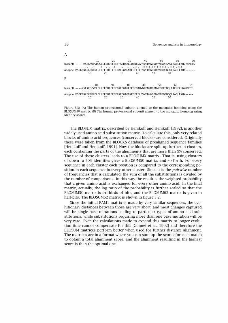
38 Sequence analysis in immunology
A
10 20 30 40 50 60 70humanD -----MSEKKQPVDLGLLEEDDEFEEFPAEDWAGLDEDEDAHVWEDNWDDDNVEDDFSNQLRAELEKHGYKMETS
..: . : :.:. : . .. ...:. :::::::::::::::..::::.::::Anophe MSDKENKDKPKLDLGLLEEDDEFEEFPAEDWAGNKEDEEELSVWEDNWDDDNVEDDFNQQLRAQLEKHK------
10 20 30 40 50 60
B
10 20 30 40 50 60 70humanD ----MSEKKQPVDLGLLEEDDEFEEFPAEDWAGLDEDEDAHVWEDNWDDDNVEDDFSNQLRAELEKHGYKMETS
....:...:::::::::::::::::::::..:::..........::....:..::..........Anophe MSDKENKDKPKLDLGLLEEDDEFEEFPAEDWAGNKEDEEELSVWEDNWDDDNVEDDFNQQLRAQLEKHK-----
10 20 30 40 50 60
Figure 3.3: (A) The human proteasomal subunit aligned to the mosquito homolog using theBLOSUM50 matrix. (B) The human proteasomal subunit aligned to the mosquito homolog usingidentity scores.
The BLOSUM matrix, described by Henikoff and Henikoff [1992], is anotherwidely used amino acid substitution matrix. To calculate this, only very relatedblocks of amino acid sequences (conserved blocks) are considered. Originallythese were taken from the BLOCKS database of prealigned sequence families[Henikoff and Henikoff, 1991]. Now the blocks are split up further in clusters,each containing the parts of the alignments that are more than X% conserved.The use of these clusters leads to a BLOSUMX matrix. That is, using clustersof down to 50% identities gives a BLOSUM50 matrix, and so forth. For everysequence in each cluster each position is compared to the corresponding po-sition in each sequence in every other cluster. Since it is the pairwise numberof frequencies that is calculated, the sum of all the substitutions is divided bythe number of comparisons. In this way the result is the weighted probabilitythat a given amino acid is exchanged for every other amino acid. In the finalmatrix, actually, the log ratio of the probability is further scaled so that theBLOSUM50 matrix is in thirds of bits, and the BLOSUM62 matrix is given inhalf-bits. The BLOSUM62 matrix is shown in figure 3.2.
Since the initial PAM1 matrix is made by very similar sequences, the evo-lutionary distances between those are very short, and most changes capturedwill be single base mutations leading to particular types of amino acid sub-stitutions, while substitutions requiring more than one base mutation will bevery rare. Even the calculations made to expand this matrix to longer evolu-tion time cannot compensate for this [Gonnet et al., 1992] and therefore theBLOSUM matrices perform better when used for further distance alignment.The matrices are in a format where you can sum up the scores for each matchto obtain a total alignment score, and the alignment resulting in the highestscore is then the optimal one.

Alignments 39
3.2.3 Gap Penalties
Using the BLOSUM50 matrix to align mosquito and human proteasomeal sub-units (figure 3.3A) gives a slightly different alignment than just using aminoacid identities (figure 3.3B). These two different alignments also reveal thatthere are two parts of the proteins with a high number of identical aminoacids, but without inserting or deleting letters in one of the sequences theycannot be aligned simultaneously. This leads obviously to the necessity ofinserting gaps in the alignments.
A gap in one sequence represents an insertion in the other sequence. First,to avoid having gaps all over the alignment these have to be penalized justlike unmatching amino acids. This penalty (i.e., the probability that a givenamino acid will be deleted in another related sequence) cannot be derived fromthe database alignments used to create the PAM and BLOSUM matrices, sincethese are ungapped alignments. Instead, a general gap insertion penalty is de-termined, usually empirically, and is often lower than the lowest match score.Having only one score for any gap inserted is called a linear gap cost, andwill lead to the same total penalty for three single gaps at three different po-sitions in the alignment as having a single stretch of three gaps. This doesnot make sense biologically, however, since insertions and deletions often in-volve a longer stretch of DNA in a single event. For this reason two differentgap penalties are usually included in the alignment algorithms: one penaltyfor having a gap at all (gap opening penalty), and another, smaller penalty,for extending already opened gaps. This is called an affine gap penalty and isactually a compromise between the assumption that the insertion, or deletion,is created by one or more events. Furthermore, it is possible to let gaps ap-pended at the ends of the sequences not to have a penalty, since insertions atthe ends will have a much greater chance of not disrupting the function of aprotein. For a more careful discussion of how to set gap penalties, see Vingronand Waterman [1994].
3.2.4 Alignment by Dynamic Programming
Introducing gaps greatly increases the number of different comparisons be-tween two sequences and in the general case it is impossible to do them all.To compensate for that, several shortcut optimization schemes have beeninvented. One of the earliest schemes was developed by Needleman andWunsch [1970] and works for global alignments, i.e., alignments covering allresidues in both sequences. As an example, it is here described how to aligntwo very short sequence stretches taken from our previous proteasome align-ment. For simplicity, we will use the identity matrix (match=1, mismatch=-1)and a linear gap penalty of −2. Using the Needleman-Wunsch approach

40 Sequence analysis in immunology
Score matrix
Trace Matrix
Figure 3.4: Dynamic programming, global alignment. Step 1.

Alignments 41
Score matrix
Trace Matrix
Figure 3.5: Dynamic programming, global alignment. Step 2.

42 Sequence analysis in immunology
Score matrix
Trace Matrix
Figure 3.6: Dynamic programming, global alignment. Step 3.

Alignments 43
Score matrix
Trace Matrix
Figure 3.7: Dynamic programming, global alignment, final matrices (Needleman-Wunsch).
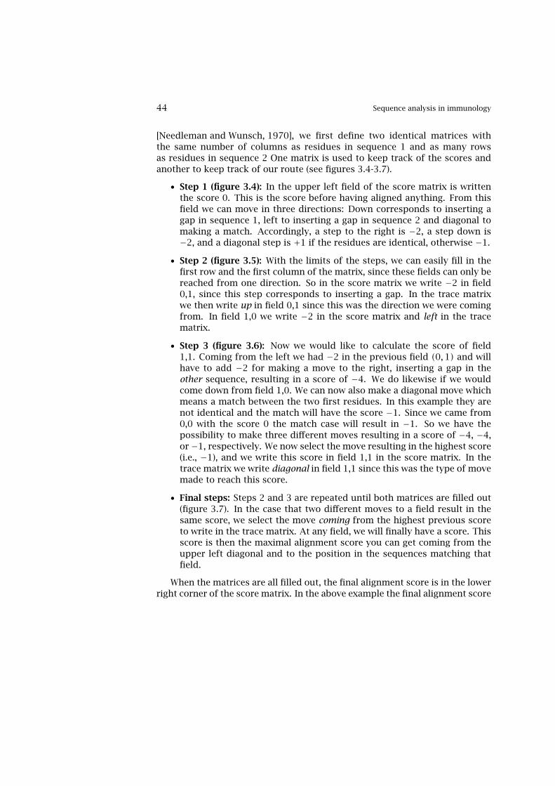
44 Sequence analysis in immunology
[Needleman and Wunsch, 1970], we first define two identical matrices withthe same number of columns as residues in sequence 1 and as many rowsas residues in sequence 2 One matrix is used to keep track of the scores andanother to keep track of our route (see figures 3.4-3.7).
• Step 1 (figure 3.4): In the upper left field of the score matrix is writtenthe score 0. This is the score before having aligned anything. From thisfield we can move in three directions: Down corresponds to inserting agap in sequence 1, left to inserting a gap in sequence 2 and diagonal tomaking a match. Accordingly, a step to the right is −2, a step down is−2, and a diagonal step is +1 if the residues are identical, otherwise −1.
• Step 2 (figure 3.5): With the limits of the steps, we can easily fill in thefirst row and the first column of the matrix, since these fields can only bereached from one direction. So in the score matrix we write −2 in field0,1, since this step corresponds to inserting a gap. In the trace matrixwe then write up in field 0,1 since this was the direction we were comingfrom. In field 1,0 we write −2 in the score matrix and left in the tracematrix.
• Step 3 (figure 3.6): Now we would like to calculate the score of field1,1. Coming from the left we had −2 in the previous field (0,1) and willhave to add −2 for making a move to the right, inserting a gap in theother sequence, resulting in a score of −4. We do likewise if we wouldcome down from field 1,0. We can now also make a diagonal move whichmeans a match between the two first residues. In this example they arenot identical and the match will have the score −1. Since we came from0,0 with the score 0 the match case will result in −1. So we have thepossibility to make three different moves resulting in a score of −4, −4,or −1, respectively. We now select the move resulting in the highest score(i.e., −1), and we write this score in field 1,1 in the score matrix. In thetrace matrix we write diagonal in field 1,1 since this was the type of movemade to reach this score.
• Final steps: Steps 2 and 3 are repeated until both matrices are filled out(figure 3.7). In the case that two different moves to a field result in thesame score, we select the move coming from the highest previous scoreto write in the trace matrix. At any field, we will finally have a score. Thisscore is then the maximal alignment score you can get coming from theupper left diagonal and to the position in the sequences matching thatfield.
When the matrices are all filled out, the final alignment score is in the lowerright corner of the score matrix. In the above example the final alignment score

Alignments 45
is then −1. The score matrix has now served its purpose and is discarded, andthe alignment is reconstructed using the trace matrix. To reconstruct the align-ment start in the lower right corner of the final trace matrix (figure 3.7). Fol-lowing the directions written in the fields, the alignment is now reconstructedbackward. Here diagonal means a match between the two last residues in eachsequence (W match W), and a move diagonal up-left. Next field: diagonal, i.e.,V match V and a move diagonal up-left. The present field value is now up: Thismeans that we introduce a gap in the first sequence to match S in the secondsequence and then move one field up in the trace matrix. The rest of the traceis all diagonal, which means no gaps, and the resulting alignment will be
DEDEDAH-VWKEDEEELSVW
This way to produce an alignment is called dynamic programming, and is stillused in major alignment software packages (e.g., the ALIGN tool in the FASTApackage uses the Needleman-Wunsch algorithm for global alignments). To il-lustrate that there are differences in the resulting alignments according towhich scoring scheme is used, the above alignment using the BLOSUM62 ma-trix in figure 3.2 and a linear gap penalty of −9 results in the following align-ment
DEDEDA-HVWKEDEEELSVW
So the optimal alignment is only optimal using the chosen substitution scoresand gap penalties, and there is no exact way to tell in a particular example ifone set of scores gives a more “correct” alignment than another set of scores.
3.2.5 Local Alignments and Database Searches
The global alignment scheme described above is very good for comparing andanalyzing the relationship between two selected proteins. Proteins, however,are often comprised of different domains, where each domain may be evo-lutionarily related to a different set of sequences. Thus when it comes tosearching for sequences it is more beneficial to only look at the parts of thesequences that actually are related. A search is actually to make pairwise align-ment of your query sequence to all the sequences in the database, and orderthe resulting alignments by the alignment score. For this purpose Smith andWaterman [1981] further developed the dynamic programming approach. TheSmith-Waterman algorithm is like Needleman-Wunsch, except that the tracesonly continue as long as the scores are positive, Whenever a score becomesnegative it is set to 0 and the corresponding trace is empty. Using the BLO-SUM62 substitution matrix and a linear gap penalty of −9, the score and trace

46 Sequence analysis in immunology
Score matrix
Trace Matrix
Figure 3.8: Dynamic programming, local alignment, final matrices (Smith-Waterman).
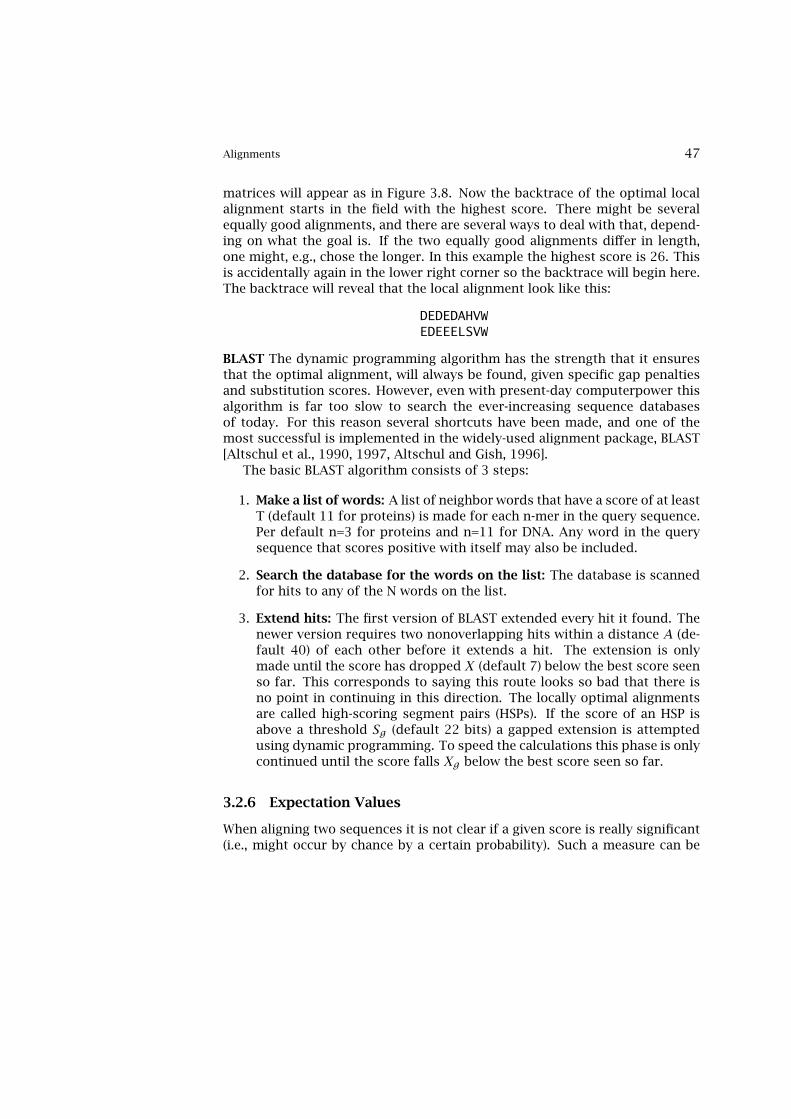
Alignments 47
matrices will appear as in Figure 3.8. Now the backtrace of the optimal localalignment starts in the field with the highest score. There might be severalequally good alignments, and there are several ways to deal with that, depend-ing on what the goal is. If the two equally good alignments differ in length,one might, e.g., chose the longer. In this example the highest score is 26. Thisis accidentally again in the lower right corner so the backtrace will begin here.The backtrace will reveal that the local alignment look like this:
DEDEDAHVWEDEEELSVW
BLAST The dynamic programming algorithm has the strength that it ensuresthat the optimal alignment, will always be found, given specific gap penaltiesand substitution scores. However, even with present-day computerpower thisalgorithm is far too slow to search the ever-increasing sequence databasesof today. For this reason several shortcuts have been made, and one of themost successful is implemented in the widely-used alignment package, BLAST[Altschul et al., 1990, 1997, Altschul and Gish, 1996].
The basic BLAST algorithm consists of 3 steps:
1. Make a list of words: A list of neighbor words that have a score of at leastT (default 11 for proteins) is made for each n-mer in the query sequence.Per default n=3 for proteins and n=11 for DNA. Any word in the querysequence that scores positive with itself may also be included.
2. Search the database for the words on the list: The database is scannedfor hits to any of the N words on the list.
3. Extend hits: The first version of BLAST extended every hit it found. Thenewer version requires two nonoverlapping hits within a distance A (de-fault 40) of each other before it extends a hit. The extension is onlymade until the score has dropped X (default 7) below the best score seenso far. This corresponds to saying this route looks so bad that there isno point in continuing in this direction. The locally optimal alignmentsare called high-scoring segment pairs (HSPs). If the score of an HSP isabove a threshold Sg (default 22 bits) a gapped extension is attemptedusing dynamic programming. To speed the calculations this phase is onlycontinued until the score falls Xg below the best score seen so far.
3.2.6 Expectation Values
When aligning two sequences it is not clear if a given score is really significant(i.e., might occur by chance by a certain probability). Such a measure can be

48 Sequence analysis in immunology
Figure 3.9: Distributions of scores, when aligning a sequence to a database of unrelated se-quences.
obtained by aligning a great number of random sequences to the original se-quence and from the resulting score distribution calculate the probability thata random sequence would result in a given score. This number is called theexpectation-value, or E-value. The random sequences is obtained by shufflingthe elements (nucleotides or amino acids) of the original sequence. In this waythe score distribution will not be biased by a skewed amino acid distributionof the original sequence.
When searching through databases the question also arises whether a givenalignment score confers a relationship between the two aligned regions or not.If we align a sequence to a database of all unrelated sequences and plot thealignment score against how many alignments will have that score we will geta curve like that in figure 3.9. This is called an extreme value distribution.We can from this distribution find out how often a given alignment-score willarise by chance. Thus the E-value is the theoretically expected number of falsehits per sequence query, and a lower E-value means a more significant hit.Importantly, the E-value is dependent on the size of the database searched asthe chance of getting a false hit rises as the database grows.
Different alignment programs use different approaches to calculate theE-value of a given database hit. FASTA actually makes all possible alignments,and returns a real distribution curve (figure 3.10) and calculates the E-value
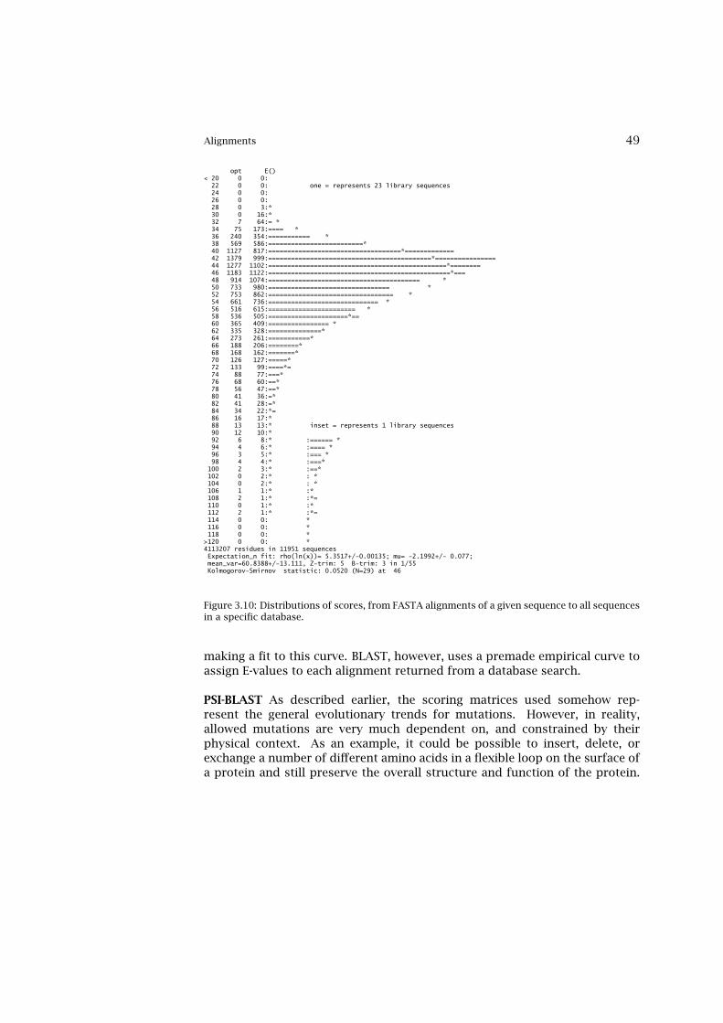
Alignments 49
opt E()< 20 0 0:
22 0 0: one = represents 23 library sequences24 0 0:26 0 0:28 0 3:*30 0 16:*32 7 64:= *34 75 173:==== *36 240 354:=========== *38 569 586:=========================*40 1127 817:===================================*=============42 1379 999:===========================================*================44 1277 1102:===============================================*========46 1183 1122:================================================*===48 914 1074:======================================== *50 733 980:================================ *52 753 862:================================= *54 661 736:============================= *56 516 615:======================= *58 536 505:=====================*==60 365 409:================ *62 335 328:==============*64 273 261:===========*66 188 206:========*68 168 162:=======*70 126 127:=====*72 133 99:====*=74 88 77:===*76 68 60:==*78 56 47:==*80 41 36:=*82 41 28:=*84 34 22:*=86 16 17:*88 13 13:* inset = represents 1 library sequences90 12 10:*92 6 8:* :====== *94 4 6:* :==== *96 3 5:* :=== *98 4 4:* :===*
100 2 3:* :==*102 0 2:* : *104 0 2:* : *106 1 1:* :*108 2 1:* :*=110 0 1:* :*112 2 1:* :*=114 0 0: *116 0 0: *118 0 0: *
>120 0 0: *4113207 residues in 11951 sequences
Expectation_n fit: rho(ln(x))= 5.3517+/-0.00135; mu= -2.1992+/- 0.077;mean_var=60.8388+/-13.111, Z-trim: 5 B-trim: 3 in 1/55Kolmogorov-Smirnov statistic: 0.0520 (N=29) at 46
Figure 3.10: Distributions of scores, from FASTA alignments of a given sequence to all sequencesin a specific database.
making a fit to this curve. BLAST, however, uses a premade empirical curve toassign E-values to each alignment returned from a database search.
PSI-BLAST As described earlier, the scoring matrices used somehow rep-resent the general evolutionary trends for mutations. However, in reality,allowed mutations are very much dependent on, and constrained by theirphysical context. As an example, it could be possible to insert, delete, orexchange a number of different amino acids in a flexible loop on the surface ofa protein and still preserve the overall structure and function of the protein.

50 Sequence analysis in immunology
A R N D C Q E G H I L K M F P S T W Y V1 I -2 -4 -5 -5 -2 -4 -4 -5 -5 6 0 -4 0 -2 -4 -4 -2 -4 -3 42 K -1 -1 -2 -2 -3 -1 3 -3 -2 -2 -3 4 -2 -4 -3 1 1 -4 -3 23 E 5 -3 -3 -3 -3 3 1 -2 -3 -3 -3 -2 -2 -4 -3 -1 -2 -4 -3 14 E -4 -3 2 5 -6 1 5 -4 -3 -6 -6 -2 -5 -6 -4 -2 -3 -6 -5 -55 H -4 2 1 1 -5 1 -2 -4 9 -5 -2 -3 -4 -4 -5 -3 -4 -5 1 -56 V -3 0 -4 -5 -4 -4 -2 -3 -5 1 -2 1 0 1 -4 -3 3 -5 -3 57 I 0 -2 -4 1 -4 -2 -4 -4 -5 1 0 -2 0 2 -5 1 -1 -5 -3 48 I -3 0 -5 -5 -4 -2 -5 -6 1 2 4 -4 -1 0 -5 -2 0 -3 5 -19 Q -2 -3 -2 -3 -5 4 -1 3 5 -5 -3 -3 -4 -2 -4 2 -1 -4 2 -2
10 A 2 -4 -4 -3 2 -3 -1 -4 -2 1 -1 -4 -3 -4 1 2 3 -5 -1 111 E -1 3 1 1 -1 0 1 -4 -3 -1 -3 0 3 -5 4 -1 -3 -6 -3 -112 F -3 -5 -5 -5 -4 -4 -4 -1 -1 1 1 -5 2 5 -1 -4 -4 -3 5 213 Y 3 -5 -5 -6 3 -4 -5 -2 -1 0 -4 -5 -3 3 -5 -2 -2 -2 7 114 L -1 -3 -4 -2 1 5 1 -1 -1 -1 1 -3 -3 1 -5 -1 -1 -2 3 -215 N -1 -4 4 1 5 -3 -4 2 -4 -4 -4 -3 -2 -4 -5 2 0 -5 0 016 P -2 4 -4 -4 -5 0 -3 3 2 -5 -4 0 -4 -3 0 1 -2 -1 5 -317 D -3 -2 1 5 -6 -2 2 2 -1 -2 -2 -3 -5 -4 -5 -1 2 -6 -3 -4
Figure 3.11: Example of a PSSM.
The corresponding number of allowed substitutions would very probably bemuch more limited in the core — or in a secondary structure, rich — regionof the protein. So if a general substitution matrix works well, a matrix repre-senting the specific evolutionary trend for a given position in a given proteinshould work even better. As described by Altschul et al. [1997], this is actuallythe case.
In the PSI-BLAST approach, first an ordinary BLAST search on the basis ofthe BLOSUM62 matrix is performed against the database. Second, a position-specific scoring matrix (PSSM) is calculated as described in chapter 4. The ma-trix is calculated by considering the substitutions observed in pairwise align-ments made between the query sequence and the hits that have an expectationvalue below a selected threshold. Now the calculated matrix (figure 3.11), asa representation of the query sequence, is used to search the database again.So when the alignment score matrix is filled out, we now look in the PSSM fora given position to find the match score between the PSSM and that particularamino acid in the database sequence. For example, if we want to match posi-tion 3 in the search sequence, a glutamic acid, to an alanine, the match score is5. However, if we want to match position 4, also a glutamic acid, to an alanine,the match score is −4. This should illustrate the higher specificity of a PSSMas compared to ordinary substitution matrices.
3.3 Multiple Alignments
When looking at several related sequences, it is often useful and informativeto look at all the sequences in one alignment (multiple alignment). The sim-plest approach is to align all the sequences, one by one, with a single selected“master sequence,” and this is what can be obtained by programs like BLAST.However, these programs make only local alignments, and often gaps and in-

Multiple Alignments 51
A
Drosophila_melanogaster MSAPDKEKEKEKEETNNKSEDLGLLEEDDEFEEFPAEDFRVGDDEEELNVWEDNWDDDNVEDDFSQQLKAHLESKKMETAnopheles_gambiae ----------DKENKDKPKLDLGLLEEDDEFEEFPAEDWAGneDEEELSVWEDNWDDDNVEDDFNQQLRAQLEKHK---Zebrafish -----------------QTVDLGLLEEDDEFEEFPAEDWTGLDEDEDAHVWEDNWDDDNVEDDFSNQLRAELE------HUMAN --------------------DLGLLEEDDEFEEFPAEDWAGLDEDEDAHVWEDNWDDDNVEDDFSNQLRAELE------MOUSE --------------------DLGLLEEDDEFEEFPAEDWAGLDEDEDAHVWEDNWDDDNVEDDFSNQLRAELE------Xenopus_laevis --------------------DLGLLEEDDEFEEFPTEDWTGFDEDEDTHVWEDNWDDDNVEDDFSNQLRAELE------Saccharomyces_cerevisiae ------------------------LEEDDEFEDFPIDTWANGETIkqTNIWEENWDDVEVDDDFTNELKAELDRYKRE-Neurospora_crassa. ----DAKSTEPKPEQPVTEKKTAVLEEDDEFEDFPVDDWEAEDTeeAKHLWEESWDDDDTSDDFSAQLKEELK------
B
Drosophila_melanogaster ----MSAPDKE----KEKEKEETNNKSEDLGLLEEDDEFEEFPAEDFRVGAnopheles_gambiae ----MS--DKEN---KDKPK-------LDLGLLEEDDEFEEFPAEDWAGNHUMAN ----MS----------EKKQ------PVDLGLLEEDDEFEEFPAEDWAGLMOUSE ----MS----------EKKQ------PVDLGLLEEDDEFEEFPAEDWAGLZebrafish ----MS----------EKKQ------TVDLGLLEEDDEFEEFPAEDWTGLXenopus_laevis ---MSS----------DKKP------PVDLGLLEEDDEFEEFPTEDWTGFNeurospora_crassa. ----MASTQPKNDAKSTEPKPEQPVTEKKTAVLEEDDEFEDFPVDDWEAESaccharomyces_cerevisiae MSTDVAAAQAQSKIDLTKKKNE----EINKKSLEEDDEFEDFPIDTWANG
: : . ********:** : :
Drosophila_melanogaster ------DDEEELNVWEDNWDDDNVEDDFSQQLKAHLESK--KMET-Anopheles_gambiae K-----EDEEELSVWEDNWDDDNVEDDFNQQLRAQLEKH--K----HUMAN ------DEDEDAHVWEDNWDDDNVEDDFSNQLRAELEKHGYKMETSMOUSE ------DEDEDAHVWEDNWDDDNVEDDFSNQLRAELEKHGYKMETSZebrafish ------DEDEDAHVWEDNWDDDNVEDDFSNQLRAELEKHGYKMETSXenopus_laevis ------DEDEDTHVWEDNWDDDNVEDDFSNQLRAELEKHGYKMETSNeurospora_crassa. DTEAAKGNNEAKHLWEESWDDDDTSDDFSAQLKEELKKVEAAKKR-Saccharomyces_cerevisiae ETIKS-NAVTQTNIWEENWDDVEVDDDFTNELKAELDRY--KRENQ
:**:.*** :..***. :*: .*.
C
HUMAN 1 ---------- ---------- ------MSEK KQPVDLGLLE EDDEFEEFPAMOUSE 1 ---------- ---------- ------MSEK KQPVDLGLLE EDDEFEEFPAZebrafish 1 ---------- ---------- ------MSEK KQTVDLGLLE EDDEFEEFPADrosophila_m 1 ----MSapDK Ek-------E KEKEET-NNK SE--DLGLLE EDDEFEEFPANeurospora_c 1 ----MA--ST QPKNDAKSTE PKPEQpVTEK KTAV----LE EDDEFEDFPVXenopus_laev 1 m--------- ---------- -----S-SDK KPPVDLGLLE EDDEFEEFPTSaccharomyce 1 mstdVA--AA QAQSKIDLTK KKNEEI-NKK S-------LE EDDEFEDFPIAnopheles_ga 1 ----MS--DK ENKD------ ---------- KPKLDLGLLE EDDEFEEFPA
HUMAN 25 EDWAGLDE-- ----DED-AH VWEDNWDDDN VEDDFSNQLR AELEK----HMOUSE 25 EDWAGLDE-- ----DED-AH VWEDNWDDDN VEDDFSNQLR AELEK----HZebrafish 25 EDWTGLDE-- ----DED-AH VWEDNWDDDN VEDDFSNQLR AELEK----HDrosophila_m 37 EDFRVGDD-- ----EEE-LN VWEDNWDDDN VEDDFSQQLK AHLES----KNeurospora_c 41 DDWEAEDtEA AKGNNEA-KH LWEESWDDDD TSDDFSAQLK EELKKveaaKXenopus_laev 26 EDWTGFDE-- ----DED-TH VWEDNWDDDN VEDDFSNQLR AELEK----HSaccharomyce 41 DTWAng--ET IKSNavtqTN IWEENWDDVE VDDDFTNELK AELDR----YAnopheles_ga 29 EDWAGNKE-- ----DEEeLS VWEDNWDDDN VEDDFNQQLR AQLEK----H
HUMAN 64 GYKMETSMOUSE 64 GYKMETSZebrafish 64 GYKMETSDrosophila_m 76 --KMET-Neurospora_c 90 --Kr---Xenopus_laev 65 GYKMETSSaccharomyce 85 --KRENQAnopheles_ga 69 --K----
Figure 3.12: Multiple alignments of the proteasome DSS1 subunit from different organismsusing A) PSI-BLAST, B) ClustalW, and C) DIALIGN. Lower case letters means a part of the sequencethat is not significantly aligned.

52 Sequence analysis in immunology
sertions will be placed differently in the master sequence depending on whichother sequence it is aligned with. Another approach is to align all sequencespairwise with all other sequences and establish the difference between everypair. Such a map is called a distance matrix, and from this it is possible to ob-tain an estimate of which sequences are most related (a cluster), and aligningthose first, and then align all the prealigned clusters against each other. This isbasically what is implemented in the most used multiple alignment program,ClustalW alias ClustalX [Thompson et al., 1994]. First is calculated a score forthe alignment between each pair of the sequences. These scores are then usedto calculate phylogenetic tree, or a dendrogram, using the clustering methodUPGMA (see Chapter 5). Having calculated the dendrogram, the sequencesare aligned in larger and larger groups. Each of these alignments consists ofaligning 2 alignments, using profile alignments, which are the alignment of 2groups of already aligned sequences. The method is an extension of the profilemethod of Gribskov et al. [1987] for aligning a single sequence with an alignedgroup of sequences. With a sequence-to-sequence alignment, a weight matrixsuch as BLOSUM62 is used to obtain a score for a particular substitution be-tween the pairs of aligned residues. In profile alignments, however, each ofthe two input alignments are treated as a single sequence, but you calculatethe score at aligned positions as the average substitution matrix score of allthe residues in one alignment vs. all those in the other, e.g., if you have 2alignments with I and J sequences respectively the score at any position is theaverage of all the I times J scores of the residues compared separately. Anygaps that are introduced are placed in all of the sequences of an alignment atthe same position. However, all gaps in the ends of the sequences are free.This might give some artifacts, especially when sequences of different lengthare aligned. Newer multiple alignment algorithms implemented in programssuch as T-Coffee [Notredame et al., 2000] and DIALIGN [Morgenstern, 1999]handle these problems much better, but the algorithms behind them will notbe described in this book. Figure 3.12 is an example of the differences in theresults, using different alignment algorithms/programs. Note that PSI-BLASTwill only return local alignments, and that the result is based on pairwise align-ments to the query sequence, i.e., no clustering has been involved.
3.4 DNA Alignments
Untill now only protein alignments have been described. The basic algorithmsand programs used for DNA alignment, however, are the same as for proteins.DNA alignments are much more difficult since at each position, we can haveone of only four different bases as opposed to one of twenty in peptide align-ments. So we will not have a specific substitution matrix like BLOSUM or PAM

Molecular Evolution and Phylogeny 53
but rather take a step back and use a general substitution score for any matchor mismatch but still using affine gap penalties. This makes the probabil-ity of any given substitution equally high, and so the significance of the finalalignment will be lower. Some nucleotide matrices, however, do have differ-ent substitution scores for transitions (Dealing with DNA/RNA sequences fromcoding regions, however, gives an opportunity to shortcut the alignment by ac-tually aligning the translation products, rather than the actual DNA sequences.This approach has been implemented in most alignment software packages, in-cluding FASTA (tfasta [Pearson and Lipman, 1988, Pearson, 1996]) and BLAST(tblast [Altschul et al., 1990, Altschul and Gish, 1996]). In this basic but strongapproach, gaps in the aligned DNA sequences will only occur in multiples oftriplets. This will, however, not catch examples correctly where frameshiftshave actually happened, leading to major changes of larger or smaller parts ofthe translated protein. For such investigations the programs GenA1 [Hein andStøvlbaek, 1994, 1996] and COMBAT [Pedersen et al., 1998] can be used, butonly for pairwise alignments. For multiple alignments an automatic methodexists that will translate DNA to peptide, do the multiple alignment using DI-ALIGN [Morgenstern, 1999], and return the final alignment at the DNA level[Wernersson and Pedersen, 2003]. Multiple DNA alignments are especially use-ful for investigating the evolution on the molecular level (molecular evolution).With such alignments it is possible to examine exactly which positions in theDNA are more or less likely to undergo mutations that survive and are trans-ferred to the progeny. We can also calculate the chance that a given codon willonly allow mutations that will not lead to an amino acid change (silent muta-tions or synonymous mutations) and compare it to the chance that a substitu-tion leads to an amino acid change (nonsynonymous mutations). This ratio iscalled dN/dS and an example of such a calculation is given in chapter 7.
3.5 Molecular Evolution and Phylogeny
Phylogenies reveal evolutionary relationships between organisms and specificsequences. In recent years molecular phylogenies have started to play a ma-jor role in epidemiological studies of pathogens. These studies provide in-formation about where and when a virulent strain can arise. Not only hu-man pathogens but also viral and bacterial disease-causing agents of livestockare of importance, as such outbreaks can cause great economic loss, as wellas increase the chance of a possible cross-species infection. Recent develop-ments of new methods for isolating, amplifying, and sequencing RNA isolatedfrom small samples of blood or tissue have made the molecular phylogeny ofpathogens a rapidly expanding research field. Moreover, since many pathogenscan mutate at much higher rates than eukaryotes, it is possible to obtain the

54 Sequence analysis in immunology
phylogeny of sequences that diverged only recently.One interesting application of molecular phylogeny is represented by anal-
ysis of the origins of HIV epidemics. Exactly when simian immunodeficiencyvirus (SIV) was transmitted from nonhuman primates to humans, giving riseto the human immunodeficiency virus (HIV), is still under investigation. Ko-rber et al. [2000] used a phylogenetic analysis of the viral sequences with aknown date of sampling to estimate the year of origin for the main group ofHIV viruses (HIV-1 M), the principal cause of acquired immunodeficiency syn-drome (AIDS). AIDS is caused by two divergent viruses, HIV-1 and HIV-2. HIV-1is responsible for the global pandemic, while HIV-2 has, until recently, been re-stricted to West Africa and appears to be less virulent in its effects. SIV virusesrelated to HIV have been found in many species of nonhuman primates. By an-alyzing the molecular divergence of the envelope gene, and applying a modelwhich assumes constant mutation rates through time and across lineages, Kor-ber et al. [2000] estimated that the last common ancestor of the HIV-1 M groupappeared in 1931 (with a confidence interval of 1916–1941). Using a differentmolecular clock analysis, where the mutation rate is allowed to change at split-ting events, and also when analyzing a different protein, the same estimateswere obtained. This approach only identifies when the common ancestor be-gan to diversify; it does not identify the exact time of transmission. Still, giventhis estimate, one is able to come up with more precise hypotheses about thetransmission event.
3.5.1 Phylogenetic Methods
The starting point of any phylogenetic work is a collection of sequences thatmight be evolutionarily related. Such a set could be extracted from publicdatabases using some of the tools described previously, or it could be datafrom one’s own work. These sequences must now be aligned by the use ofmultiple alignment software, such as ClustalW. ClustalW also calculates a dis-tance matrix of your sequences, i.e., the relation of each of your sequences tothe other sequences in your alignment. A way to visualize the distances in adistance matrix is a tree-like drawing where the distances along the branchescorrelates with the distances in the distance matrix. Such a drawing is called aphylogenetic tree. One important point about trees is that they are only usefulif the described system has been under vertical evolution (i.e., no horizontalgene transfers and recombination), otherwise a simple tree makes no sense.To calculate the grouping and the branch lengths of such a tree, two majorapproaches are applicable. One approach is optimization methods that willfind the tree that gives the optimal fit to the matrix, e.g., the minimal sum ofsquared errors. Another approach is clustering methods that is related to the

Viral Evolution and Escape: Sequence Variation 55
optimization methods, but is much faster. The clustering methods, however,do not guarantee the optimal solution.
Two major types of trees exist: rooted and unrooted trees. With rootedtrees a common ancestor point is used as the origin of the tree, no matter ifthis is really scientific sane with the given data. In rooted trees the horizontaldistance from the leaves to the origin is directly proportional to the amountof changes. Unrooted trees are used to show relations where no common an-cestor is given, and only the evolutionary distance between the leaves can beinferred. In both rooted and unrooted trees, the leaves are grouped in clusters.This grouping depends heavily on the algorithm used. Some algorithms justgive one of potentially many, more or less equally probable, outputs. Other ap-proaches actually calculate many different solutions and give the most proba-ble outcome with some indication of how reliable a particular solution is.
As a simple example, we will investigate the phylogenetic relationship be-tween HIV and SIV using a set consisting of 27 different gp120 protein se-quences from isolates of HIV-1, HIV-2, chimpanzee SIV, and macaque monkeySIV. The gp120 protein of HIV is crucial for binding of the virus particle totarget cells. It is the specific affinity of gp120 for the CD4 protein that targetsHIV to those cells of the immune system that express CD4 on their surface(e.g., helper T lymphocytes, monocytes, and macrophages). ClustalW is usedto align the sequences (figure 3.13) and, as mentioned earlier, ClustalW alsoclusters the most related sequences. The information from this clustering cansubsequently be used to produce a phylogenetic tree (figure 3.14).
The phylogenetic tree from the analysis (see figure 3.14) shows two sep-arate clusters. One contains SIV from chimpanzee (SIVCZ) together with theHIV-1 sequences, while the other contains SIV from macaque/sooty mangabeytogether with HIV-2. This indicates that HIV-1 originated from one event wherethe virus was transmitted from (presumably) chimpanzee to human, while HIV-2 originated from a second, independent event where the virus was transmit-ted from (presumably) macaque to human.
3.6 Viral Evolution and Escape: Sequence Variation
Coexistence of pathogens with their hosts imposes an evolutionary pressureboth for the host immune systems and the pathogens. The coexistence de-pends on a delicate balance between the replication rate of the pathogen andthe clearance rate by the host immune response. Throughout the animal andplant kingdoms we see several quite different strategies developed by thehost immune systems to defend themselves against intruders. Similarly, thepathogens have developed an array of immune evasion mechanisms to escapetheir elimination by the host’s immune system.
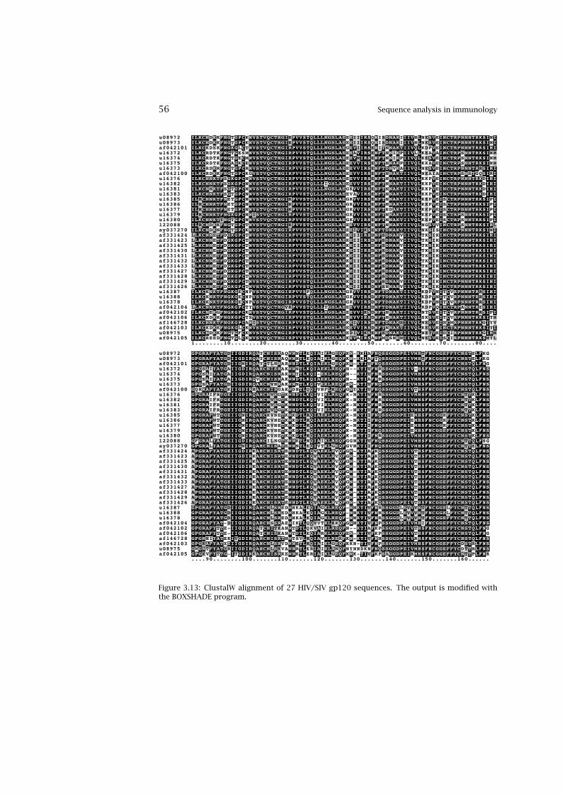
56 Sequence analysis in immunology
u08972 ILKCNDKKFNGTGPCKNVSTVQCTHGIKPVVSTQLLLNGSLAEEEIIIRSQNISDNAKIIIVHLNESVEINCTRPNNNTRKSINIu08973 ILKCNDKKFNGTGPCKNVSTVQCTHGIKPVVSTQLLLNGSLAEEEIIIRSQNISDNAKIIIVHLNESVEINCTRPNNNTRKSINIaf042101 ILKCKDEKFNGKGLCTNVSTVQCTHGIRPVVSTQLLLNGSLAEGEVIIRSENITNNAKTIIVQLKDPVEINCTRPNNNTRKSIHIu16372 ILKCRDTKFNGTGESMNVSTVQCTHGIRPVVSTQLLLNGSLAEEEAVIRSENFTNNIKPIIVLLKEAVAINCTRPSNNTRKSINMu16374 ILKCRDTKFNGTGECMNVSTVQCTHGIRPVVSTQLLLNGSLAEEEVMIRSENFTNNIKPIIVQLKESVEINCTRPSNNTRKSINMu16375 ILKCRDTKFNGAGKCENVSTVQCTHGIRPVVSTQLLLNGSLAEEEVVIRSENFTNNAKPIIVQLKKAVEINCTRPSNNTRKSINMu16373 ILKCRDKRFNGTGPCRNVSTVQCTHGIRPVVSTQLLLNGSLAEEEVVIRSENFTDNVKAIIVQLNESVEINCTRPNNNTRRSIHIaf042100 ILKCRDKKFNGTGPCKGVSTVQCTHGIRPVVSTQLLLNGSLAEEEVVIRSENFTNNAKTIIVQLNEAIAINCTRPSNSTGQSIRIu16376 ILKCNNKTFSGKGPCNNVSTVQCTHGIRPVVSTQLLLNGSLAEEEVVIRSENFTNNAKTIIVQLKKPVEINCTRPNNNTRKDIHIu16382 ILKCNNKTFSGKGPCNNVSTVQCTHGIRPVVSTQLLLIGSLAEEEVVIRSENFTNNAKTIIVQLKKPVEINCTRPNNNTRKDIHIu16381 ILKCNHKTFSGTGPCNNVSTVQCTHGIRPVVSTQLLLNGSLAEGKVVIRSENFTNNAKTIIVQLKKPVEINCTRPNNNTRKDIHIu16383 ILKCNNKTFSGTGPCNNVSTVQCTHGIRPVVSTQLLLNGSLAEEVAVIRSENFTNNAKTIIVQLKKPVEINCTRPNNNTRKDIHIu16385 ILRCNNKTFNETGPCNNVSTVQCTHGIKPVVSTQLLLNGSLAEGKVVIRSENFTNNAKTIIVQLKEPVEISCTRPNNNTRKSIPIu16386 ILRCNNKTFNETGPCNNVSTVQCTHGIKPVVSTQLLLNGSLAEGKVVIRSENFTNNAKTIIVQLKEPVEISCTRPNNNTRKSIPIu16377 ILRCNNKTFNETGPCNNVSTVQCTHGIKPVVSTQLLLNGSLAEGKVVIRSENFTNDAKTIIVQLKEPVEISCTRPNNNTRKSIPIu16379 ILRCNNKTFNGKGPCNNISTVQCTHGIRPVVSTQLLLNGSLAEGKVVIRSENFTNNAKTIIVQLKEPVEISCTRPSNNTRKSIPIu16380 ILKCNNKTYNGTGPCNNVSTVQCTHGIRPVVSTQLLLNGSLAEGKVVIRSENFTNNAKTIIVQLKEPVEISCTRPSNNTRKSIPIl22088 ILRCNDKKFNGTGPCTNVSTVQCTHGIKPVVSTQLLLNGSLAEEEVVIRSENFTNNAKTIIVQLNGSVVINCTRPSNNTRKSIHLay037270 ILKCNDKNFNGTGPCKNVSTVQCTHGIRPVVSTQLLLNGSLAEEEIVIKSENFTDNAKTIIVQLNKSISINCTRPNNNTRKSINIaf331424 LLKCNNETFDGKGPCTNVSTVQCTHGIRPVVSTQLLLNGSLAEKEIIIRSDNFSDNAKVIIVQLTKSIKINCTRPNNNTRKSIHIaf331423 LLKCNNETFDGKGPCTNVSTVQCTHGIRPVVSTQLLLNGSLAEKEIIIRSDNFSDNAKVIIVQLTKSIKINCTRPNNNTRKSIHIaf331425 LLKCNNETFDGKGPCTNVSTVQCTHGIRPVVSTQLLLNGSLAEKEIIIRSDNFSDNAKVIIVQLTKSIKINCTRPNNNTRKSIHIaf331430 LLKCNNETFDGKGPCTNVSTVQCTHGIRPVVSTQLLLNGSLAEKEIIIRSDNFSDNAKVIIVQLTKSIKINCTRPNNNTRKSIHIaf331431 LLKCNNETFDGKGPCTNVSTVQCTHGIRPVVSTQLLLNGSLAEKEIIIRSDNFSDNAKVIIVQLTKSIKINCTRPNNNTRKSIHIaf331432 LLKCNNETFDGKGPCTNVSTVQCTHGIRPVVSTQLLLNGSLAEKEIIIRSDNFSDNAKVIIVQLTKSIKINCTRPNNNTRKSIHIaf331433 LLKCNNETFDGKGPCTNVSTVQCTHGIRPVVSTQLLLNGSLAEKEIIIRSDNFSDNAKVIIVQLTKSIKINCTRPNNNTRKSIHIaf331427 LLKCNNETFDGKGPCTNVSTVQCTHGIRPVVSTQLLLNGSLAEKEIIIRSDNFSDNAKVIIVQLTKSIKINCTRPNNNTRKSIHIaf331428 LLKCNNETFDGKGPCTNVSTVQCTHGIRPVVSTQLLLNGSLAEKEIIIRSDNFSDNAKVIIVQLTKSIKINCTRPNNNTRKSIHIaf331429 LLKCNNETFDGKGPCTNVSTVQCTHGIRPVVSTQLLLNGSLAEKEIIIRSDNFSDNAKVIIVQLTKSIKINCTRPNNNTRKSIHIaf331426 LLKCNNETFDGKGPCTNVSTVQCTHGIRPVVSTQLLLNGSLAEKEIIIRSDNFSNNAKVIIVQLTKSIKINCTRPNNNTRKSIHIu16387 ILKCKNKTFNGKGECNPVSTVQCTHGIRPVVSPQLLLNGSLAEGKVVIRSDNFTDNAKTIIVQLKDPVNITCVRPNNNTRRSIHIu16388 ILKCKNKTFNGKGECNPVSTVQCTHGIRPVVSTQLLLNGSLAEGKVVIRSDNFTDNAKTIIVQLKDPVNITCVRPNNNTRRSIHIu16378 ILKCKNKTFNGKGECNPVSTVQCTHGIRPVVSTQLLLNGSLAEGKVVIRSDNFTDNAKTIIVQLKDPVNITCVRPNNNTRRSIHIaf042104 LLKCNNKTFNGKGPCTYVSTVQCTHGVKPVVSTQLLLYGSLAEEEVVIRSDNFTDNAKTIIVQLRDPVQINCTRPANNTRESIHIaf042102 ILKCNEKGFNGKGPCKNVSTVQCTHGIRPVVSTQLLLNGSLAEEEVVIKSDNFTNNAKTIIVQLNTSVEITCVRPNNNTRRSIPIaf042106 ILKCKDKRFNGKGPCTSVSTVQCTHGIRPVVSTQLLLNGSLAEEEVVIRSDNFTNNAKTIIVQLSKSVEITCVRPNNNTRKSITMaf146728 ILKCNNKTFNGKGPCANISTVQCTHGIRPVVSTQLLLNGSLAEKEIVIRSDNFTDNAKSIIVQLNESVEIHCMRPNNNTRKGIYVaf042103 ILKCKDKKFNGKGLCKNVSTVQCTHGIRPVVSTQLLLNGSLAEEEVVIRSDNFTNNAKTIIVQLKESVKINCTRPNNNTRKSITIu08975 ILKCNDKKFNGTGFCKNVSTVQCTHGIRPVVSTQLLLNGSLAEEDIVIKSENFSDNAKTIIVQLNETVKIDCIRPNNNTRKGIHMaf042105 ILKCREEDFNGTGLCKNVSTVQCTHGIRPVVSTQLLLNGSLAEKEVAIRSANFMDSNKNIIVQLNESVKISCIRPNNNTRKSMTL 1........10........20........30........40........50........60........70........80....
u08972 GPGRAFYATGDIIGDIRQAYCNISRAQWNNTLEQIAIKLGEQFKN-KKIAFNQSSGGDPEIVMHTFNCGGEFFYCNSTELFKGu08973 GPGRAFYATGDIIGDIRQAYCNISRAQWNNTLEQIAIKLGEQFKN-KKIAFTQSSGGDPEIVMHTFNCGGEFFYCNSTELFKGaf042101 GPGRAFYATGDIIGNIRQAYCTLNRARWNDTLKQIAEKLGEQFKN-KTIVFNQSSGGDPEIVMHSFNCGGEFFYCNSTQLFNGu16372 GPGSAIYATGAIIGDIRQAHCNISRAKWNNTLKQIAEKLREQFN--KTIVFNRSSGGDPEIV-HSFNCGGEFFYCNSTQLFNSu16374 GPGSAIYATGAIIGDIRQAHCNISRAKWNTTLKQI-EKLREQFN--KTIVFNRSSGGDPEIVMHSFNCGGEFFYCNSTQLFNSu16375 GPGSAIYATGAIIGDIRQVHCNISRAKWNDTLKQIAEKLREQFN--KTIAFNRSSGGDPEIVMHSFNCGGEFFYCNSTQLFNSu16373 GPGSAFYATGDIIGDIRQAHCNVNRAKWNNTLKQIVEKLREQFEN-KTIVFNQSSGGDPEIVMHSFNCGGEFFYCNSTQLFNSaf042100 GQRRAFYATGKIIGDIRHAHCNISGAKWDNTLQQIVNFLKEQFGNYKTIVFNQSSGGDPEIVTHSFNCGGEFFYCNSTQLFNSu16376 GPGRAIFRTGEIIGDIRQAHCNVSGTKWNDTLKQIVIKLREQFK-NKTIVFNRSSGGDPEIVMHSFNCGGEFFYCNTTKLFNSu16382 GPGRAIFRTGEIIGDIRQAHCNVSGTKWNDTLKQIVIKLREQFK-NKTIVFNRSSGGDPEIVMHSFNCGGEFFYCNTTKLFNSu16381 GPGRAIFRTGEIIGDIRQAHCNVSGTKWNDTLKQIVIKLREQFK-NKTIVFNRSSGGDPEIVMHSFNCGGEFFYCNTTKLFNSu16383 GPGRAIFRTGEIIGDIRQAHCNVSGTKWNDTLKQIVIKLREQFK-NKTIVFNRSSGGDPEIVMHSFNCGGEFFYCNTTKLFNSu16385 GPGRAFWTTGEIIGNIRQAHCKVNETKWKDTLRQIAEKLREQFK-NKTIIFNQSSGGDPEIEMHSFNCGGKFFYCNSTKLFNSu16386 GPGRAFWTTGEIIGNIRQAHCKVNETKWKDTLRQIAEKLREQFK-NKTIIFNQSSGGDPEIEMHSFNCGGKFFYCNSTKLFNSu16377 GPGRAFWTTGEIIGNIRQAHCKVNETKWKDTLRQIAEKLREQFK-NKTIIFNQSSGGDPEIEMHSFNCGGKFFYCNSTKLFNSu16379 GPGRAFWTTGEIIGNIRQAHCKVNETKWKDTLRQIAEKLREQFK-NKTIIFNQSSGGDPEIEMHSFNCGGEFFYCNSTKLFNSu16380 GPGRAFWTTGEIIGNIRQAHCKVNETKWKDTLRQIAEKLREQFK-NKTIIFNRSSGGDPEIVMHSFNCGGEFFYCNSTKLFNSl22088 GFGRALYATGEIIGDIRQAHCILNGTEWNKTLNQIAIKLREQFGGNKTIVFNQSSGGDPEIVMHSFNCGGEFFYCNTTQLFSGay037270 GPGRALYATGEIIGNIRQAHCNISATEWNNTLEQIVTKLGEQFGVNKTIIFNQSSGGDPEIVMHSFNCGGEFFYCNTTELFNSaf331424 APGRAFYATGEIIGDIRKAHCNISRTEWNDTLKQVAEKLRVQFGN-KTIAFKQSSGGDPEIVTHSFNCGGEFFYCNSTQLFNSaf331423 APGRAFYATGEIIGDIRKAHCNISRTEWNDTLKQVAEKLRVQFGN-KTIAFKQSSGGDPEIVTHSFNCGGEFFYCNSTQLFNSaf331425 APGRAFYATGEIIGDIRKAHCNISRTEWNDTLKQVAEKLRVQFGN-KTIAFKQSSGGDPEIVTHSFNCGGEFFYCNSTQLFNSaf331430 APGRAFYATGEIIGDIRKAHCNISRTEWNDTLKQVAEKLRVQFGN-KTIAFKQSSGGDPEIVTHSFNCGGEFFYCNSTQLFNSaf331431 APGRAFYATGEIIGDIRKAHCNISRTEWNDTLKQVAEKLRVQFGN-KTIAFKQSSGGDPEIVTHSFNCGGEFFYCNSTQLFNSaf331432 APGRAFYATGEIIGDIRKAHCNISRTEWNDTLKQVAEKLRVQFGN-KTIAFKQSSGGDPEIVTHSFNCGGEFFYCNSTQLFNSaf331433 APGRAFYATGEIIGDIRKAHCNISRTEWNDTLKQVAEKLRVQFGN-KTIAFKQSSGGDPEIVTHSFNCGGEFFYCNSTQLFNSaf331427 APGRAFYATGEIIGDIRKAHCNISRTEWNDTLKQVAEKLRVQFGN-KTIAFKQSSGGDPEIVTHSFNCGGEFFYCNSTQLFNSaf331428 APGRAFYATGEIIGDIRKAHCNISRTEWNDTLKQVAEKLRVQFGN-KTIAFKQSSGGDPEIVTHSFNCGGEFFYCNSTQLFNSaf331429 APGRAFYATGEIIGDIRKAHCNISRTEWNDTLKQVAEKLRVQFGN-KTIAFKQSSGGDPEIVTHSFNCGGEFFYCNSTQLFNSaf331426 APGRAFYATGEIIGDIRKAHCNISRTEWNDTLKQVAEKLRVQFGN-KTIAFKQSSGGDPEIVTHSFNCGGEFFYCNSTQLFNSu16387 GPGRAFYATGDIIGDIRQAHCNLSREDWHKALEQIAGKLREQF-NNKTIVFNRSSGGDLEVVVHTFNCGGELFYCNTTQLFNSu16388 GPGRAFYATGDIIGDIRQAHCNLSREDWHKALEQIAGKLREQF-NNKTIVFNRSSGGDLEVVVHTFNCGGELFYCNTTQLFNSu16378 GPGRAFYATGDIIGDIRQAHCNLSREDWHKALEQIAGKLREQF-NNKTIVFNRSSGGDLEVVVHTFNCGGEFFYCNTTQLFNSaf042104 GPGRAFYAT-DIIGDIRQAHCNSSRAEWIKTLQQVVTKLKKQFGNNKTIVFNPSSGGDPEIVMHIFNCGGEFFYCNSTQLFNSaf042102 GPGRAFYTTE-IIGDIRQAYCNITKANWTDTLQKVAIKLREQFN--KTIAFKPSSGGDPEIVTHSFNCGGEFFYCNSTQLFNGaf042106 GPGRAFYTTE-IIGDIRQAYCNISKANWTDTLEQIARKLREQFEN-KTIVFKPSSGGDPEIVTHSFNCGGEFFYCNSTQLFNGaf146728 GPGRHIYATEKIVGDIRQAHCNISRTNWTSVLRQIAVKLRERFKN-KTIVFNHSSGGDPEIVRHSFNCGGEFFYCNSTQLFNSaf042103 GPGKAFYATXEIIGDIRQAHCNLSRVDWNETLRQIAIKLGEQFKKN-TIVFNPSSGGDPEIVMHSFNCGGEFFYCDSTRLFNSu08975 GWGRTFYATGRIIGDIRQAHCNLSKVAWNRTLERIAIKLRNQFNYNNDKNFNQSSGGDPEIVMHSFNCGGEFFYCDTTHLFNSaf042105 GPGKVFYTTG-ITGDIRKAHCNISRKEWNKTLERIAIKLGEQFKNK-TIVFKPSAGGDPEIKMHSFNCGGEFFYCNTTPLFNR ....90........100.......110.......120.......130.......140.......150.......160......
Figure 3.13: ClustalW alignment of 27 HIV/SIV gp120 sequences. The output is modified withthe BOXSHADE program.

Viral Evolution and Escape: Sequence Variation 57
Figure 3.14: A rooted tree of 27 aligned HIV/SIV gp120 sequences. HV1XX=HIV-1 sequences,HV2XX=HIV-2 sequences, SIVMX=SIV (macaque), SIVSX=SIV (sooty mangabey), SIVCZ=SIV (chim-panzee).
We can divide the immune evasion mechanisms (mainly of viruses) broadlyinto three categories that allow:
1. avoiding the humoral immune response,
2. interfering with the cellular immune response,
3. disrupting the immune effector functions, e.g., by expressing some cy-tokines.

58 Sequence analysis in immunology
The humoral response is impaired whenever the antibody binding sites ona protein (often on the surface) mutate in such a way that binding is no longerpossible. Especially neutralizing antibodies, i.e., the antibodies that can blockinfection of the cells by the pathogen, cause a high selection pressure on thevirus to mutate. The most straightforward way of identifying such mutantsis via sequence analysis of the pathogenic samples. The first step is to alignthe sequences to pinpoint which regions of the pathogen are mutating. Thismay be the region that is under the strongest selection pressure by the anti-bodies. However, it could also be areas with no constrains. Such alignmentsdemonstrate that the most typical examples of escape from antibody responseoccur in the influenza virus and HIV. The human body can rapidly mount neu-tralizing antibodies against the major surface protein of the influenza surfaceprotein, hemagglutinin. The influenza virus evades this humoral response bytwo mechanisms [Gorman et al., 1992]. First, using point mutations, the vi-ral variants can escape neutralization, but this does not cause severe disease,since there will still be some unaltered epitopes that can be recognized. Sec-ond, if RNA segments are exchanged between different strains, the hemagglu-tinin protein can gain a totally different structure. In such a case, the anti-bodies made during previous infections are no longer functional and severepandemics can occur [Claas and Osterhaus, 1998]. Interestingly, the phyloge-netic analysis of the hemagglutinin protein shows that the antigenic evolutionof the influenza virus is punctuated, i.e., some mutants cause epidemics foralmost eight consecutive years, while others last only for two or three years[Smith et al., 2004]. Since the 1960s (when the first sequences were collected)every viral mutant has been able to cause an epidemic for at least two years,after which enough individuals will have acquired immunity to limit the spreadsignificantly (herd immunity).
Similarly, the cytotoxic T lymphocyte (CTL) response can be abrogatedwhenever peptide binding of MHC molecules or binding of the T cell receptorto the MHC-peptide complex is disturbed. It is relatively difficult to observesuch escapes, because they are different for each individual, depending on heror his MHC background. Therefore many CTL escape variants can be circulat-ing in a host population without one becoming the dominant mutant. Only inchronic infections like HIV and hepatitis B is it possible to find these escapemutants in a patient. Again, for HIV we have an extensive amount of data toanalyze CTL escape mutants. Using sequence analysis it is possible to see thatescape mutations are not spread all over the viral genome, because HIV is notable to tolerate changes equally well in all proteins. HIV has very flexible pro-teins like the envelope protein, gp160, where up to 35% of the sequence canbe different from the wild-type virus [Gaschen et al., 2002]. On the other hand,for some proteins, like capsid protein p24, the surface cannot tolerate pointmutations without a severe loss of viral fitness [von Schwedler et al., 2003,
Prediction of Functional Features of Biological Sequences 59
Leslie et al., 2004].An effective vaccine should be able to target the parts of a pathogenic
genome that are quite conserved even under the above-mentioned selectionpressures. For example, given that less than a 2% amino acid change can causea failure in cross-reactive immunity of the influenza vaccine [Korber et al.,2001b], it is obvious that for an HIV vaccine to use the envelope protein wouldbe futile. One approach to deal with such large diversity is to use the consen-sus or the ancestral virus sequence as a vaccine. Such sequences have the ad-vantage of being central and most similar to circulating strains. Another, saferapproach would be to design epitope vaccines, which again requires choosingthe most conserved epitopes. But the selection of such epitopes also requirescomputational analysis that goes beyond what simple sequence comparisontechniques can handle, as the binding specificities are influenced by correla-tions between amino acids present at different peptide positions. A solutionto this problem is to use machine learning techniques (see chapter 5).
3.7 Prediction of Functional Features of Biological Sequences
During experimental analysis of the immune system, proteins of unknownfunction are typically being identified as key players using high-throughputgene expression or proteomics data. The functional assignment of such im-mune system–related proteins also often requires sequence analysis that goesbeyond what can be solved by simple sequence alignment methods. In mostgenomes no more than 40 to 60% of the proteins can be assigned a functionalrole based on sequence similarity to proteins with known function. Tradi-tionally, protein function has been related directly to the 3D structure of theprotein chain of amino acids, which currently, for an arbitrary sequence, isquite hard (in the general case, impossible) to compute. As the sequence,in a given biochemical context, determines the structure, functional informa-tion between two sequences can be transferred by comparing the sequence ofamino acids by aligning the two against each other. This method is fast andpowerful, but only solves part of the problem: it is still impossible to deter-mine that two quite different sequences encode proteins with essentially thesame biochemical function.
Several different methods have been developed which do not rely on di-rect sequence similarity, but on features which go beyond sequence-wide sim-ilarity, such as the gene position in the genome, or integration of local orglobal protein features. One such method, ProtFun, does not, like sequencealignment, compare any two sequences, but operates in the “feature” spaceof all sequences. ProtFun is therefore complementary to methods based onalignment and the inherent, position-by-position quantification of similarity
60 Sequence analysis in immunology
between two sequences and their amino acids [Jensen et al., 2002, 2003]. Thisparticular method is still entirely sequence-based and does not require priorknowledge of gene expression, gene fusion, or protein-protein interaction.
For any function assignment method, the ability to correctly predict thefunctional relationship depends strongly on the function classification schemeused. One would, e.g., not expect that a method based on coregulation of geneswill work well for a category like "enzyme," since enzymes and the genes cod-ing for their substrates or substrate transporters often display strong coregu-lation at the gene and protein levels.
The ProtFun approach to function prediction is based on the fact that aprotein is not alone when performing its biological task. It will have to oper-ate using the same cellular machinery for modification and sorting as all theother proteins do. Essential types of post-translational modifications (PTMs)include glycosylation, phosphorylation, and cleavage of N-terminal signal pep-tides controlling the entry to the secretory pathway, but hundreds of othertypes of modification exist (a subset of these will be present in any given or-ganism). Many of the PTMs are enabled by local consensus sequence motifs,while others are characterized by more complex patterns of correlation be-tween the amino acids close or far apart in the sequence.
This suggests an alternative approach to function prediction, as one mayexpect that proteins performing similar functions would share some attributeseven though they are not at all related at the global level of amino acid se-quence. As several powerful predictive methods for PTMs and localizationhave been constructed, a function prediction method based on such attributescan be applied to all proteins where the sequence is known.
3.7.1 The ProtFun Method
The ProtFun method integrates (using an artificial neural network approach;see chapter 5 for a general introduction) many individual attribute predictionsand calculated sequence statistics (out of many more tested for discriminativevalue) (see figure 3.15). The integrated method predicts functional categorieswhich can be defined in various ways. The method predicts, e.g., whether a se-quence is likely to function as an enzyme, and if so, its category according tothe classes defined by the Enzyme Commission. The same scheme can be usedto predict any other set of functional classes, including highly specific ones,such as "ligand gated ion channel." It can, for example, be used to identify hor-mones, growth factors, receptors, and ion channels in the human genome asdefined by the Gene Ontology Consortium gene function classification scheme.Obviously, even though such methods produce predictions with false positivesand false negatives, they can provide essential clues, e.g., to selecting an assay
Prediction of Functional Features of Biological Sequences 61
if the confidence scores are sufficiently high.The method uses combinations of attributes as input to the neural network
for predicting the functional category of a protein. Combinations of attributescan be selected by evaluating their discriminative value for a specific functionalcategory, say proteins involved in transcription or proteins being transporters.Attributes useful for function prediction must not only correlate well withthe functional classification scheme, but must also be predictable from thesequence with reasonable accuracy.
Interestingly, the combinations of attributes selected for a given categoryalso implicitly characterize a particular functional class in an entirely new way.This type of method identifies, without any a priori ranking of their impor-tance, the biological features relevant to a particular type of functionality, sayattributes which are discriminative for two different categories of ion channels.
The success of the method indicates that (even predicted) PTMs correlatestrongly with the functional categories and this fits well with general biologi-cal knowledge. For proteins with “regulatory function” one of the most impor-tant features turned out to be phosphorylation, consistent with the fact thatreversible phosphorylation is a well-known and widely used regulatory mecha-nism. Glycosylation was also found to be a strong indicator for regulatory pro-teins. The most important single feature for distinguishing between enzymesand nonenzymes turned out to be predicted protein secondary structure. Thisalso makes sense, as enzymes are known to be overrepresented among all-alpha proteins where the amino acid chain forms an alpha-helix structure, andmore rarely are found to be all-β proteins, where the structure is rich in β-sheet.
3.7.2 Individual Sequence Prediction
The ProtFun method can be used to characterize the entire genome, but it isperhaps best suited for obtaining functional hints for individual sequences forlater use in assay selection and design. As an example we can take the humanprion sequence which is being associated with the Creutzfeldt-Jacob disease.The functionality of this protein, which seems to produce no phenotype whenknocked out in mice, was for a long time not fully understood. The ProtFunmethod predicts (see figure 3.16) with high confidence that the human prionsequence belongs to the transport and binding category, and also that it is veryunlikely to be an enzyme. Indeed, prions have now been shown to be able tobind and transport copper, while no catalytic activity has ever been observed.Interestingly, as the prion is a cell surface glycoprotein (expressed by neuralcells) it has a distinct pattern of post-translational modification, which mostlikely contains information which can be exploited by the prediction method

62 Sequence analysis in immunology
Figure 3.15: The ProtFun neural networks that predict the function of proteins in protein featurespace. Each sequence is converted into features and then the networks (NN) integrate thesefeatures and provide a prediction for the affinity toward different functional categories. Fordifferent categories different protein features will have discriminatory value. During training(using experimentally characterized data) the most discriminative features are determined foreach category.
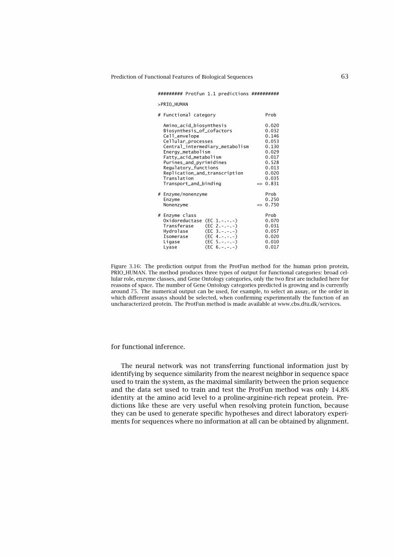
Prediction of Functional Features of Biological Sequences 63
######### ProtFun 1.1 predictions ##########
>PRIO_HUMAN
# Functional category Prob
Amino_acid_biosynthesis 0.020Biosynthesis_of_cofactors 0.032Cell_envelope 0.146Cellular_processes 0.053Central_intermediary_metabolism 0.130Energy_metabolism 0.029Fatty_acid_metabolism 0.017Purines_and_pyrimidines 0.528Regulatory_functions 0.013Replication_and_transcription 0.020Translation 0.035Transport_and_binding => 0.831
# Enzyme/nonenzyme ProbEnzyme 0.250Nonenzyme => 0.750
# Enzyme class ProbOxidoreductase (EC 1.-.-.-) 0.070Transferase (EC 2.-.-.-) 0.031Hydrolase (EC 3.-.-.-) 0.057Isomerase (EC 4.-.-.-) 0.020Ligase (EC 5.-.-.-) 0.010Lyase (EC 6.-.-.-) 0.017
Figure 3.16: The prediction output from the ProtFun method for the human prion protein,PRIO_HUMAN. The method produces three types of output for functional categories: broad cel-lular role, enzyme classes, and Gene Ontology categories, only the two first are included here forreasons of space. The number of Gene Ontology categories predicted is growing and is currentlyaround 75. The numerical output can be used, for example, to select an assay, or the order inwhich different assays should be selected, when confirming experimentally the function of anuncharacterized protein. The ProtFun method is made available at www.cbs.dtu.dk/services.
for functional inference.
The neural network was not transferring functional information just byidentifying by sequence similarity from the nearest neighbor in sequence spaceused to train the system, as the maximal similarity between the prion sequenceand the data set used to train and test the ProtFun method was only 14.8%identity at the amino acid level to a proline-arginine-rich repeat protein. Pre-dictions like these are very useful when resolving protein function, becausethey can be used to generate specific hypotheses and direct laboratory experi-ments for sequences where no information at all can be obtained by alignment.

64 Sequence analysis in immunology
3.7.3 Predicting Functional Categories for Systems Biology: the CellCycle as an Example
Characterization of the immune system also requires that genes and proteinsare grouped into subsystems, where the biochemical task of each protein maybe highly different. The ProtFun method can also be used to group sequencesin this manner. As an example with relevance for the immune system, we de-scribe here a version of the method that predicts whether a protein is encodedby a periodically transcribed, cell cycle regulated gene, or not. The ability of acell to replicate itself is one of the most fundamental features of life, and alsoof disease, most importantly in relation to cancers. The hundreds of genesmaintaining the cell cycle work together in a highly robust manner, making itpossible for cells to divide under many different growth conditions and otherinfluences from the environment. The robustness is achieved by sophisticatedregulation making the periodic gene expression highly stable. The eukary-otic cell cycle is regulated at many levels, from transcription and translationto posttranslational modification and targeted protein degradation. Proteinsneed not only be produced, but also be removed again when no longer needed.The cell cycle molecular machinery consists of highly diverse proteins, withlittle sequence similarity.
A key technique being used to elucidate which genes are involved in a givensubsystem is the DNA microarray method (see section 5.1). This is also thecase for the cell cycle, where gene expression measurements are made duringmany different time points of the cycle. Unfortunately, many of the “lists”of genes, which have been produced in this way do not agree as much asexpected, even if these studies have produced highly valuable informationde Lichtenberg et al. [2003, 2004]. Part of the disagreement relates to dif-ferences in experimental conditions and procedures, but a large fraction ispresumably related to basic noise problems in the DNA microarray technologywhen measuring the expression level of weakly expressed genes.
The ProtFun function classification technique described above can be usedto predict, in feature space, such systems biology related categories de Lichten-berg et al. [2003]. Not all cell cycle related genes are periodic, but many of thekey factors enabling the final formation of protein complexes are. The fact thatthe method with a reasonable high performance is able to separate such twohighly diverse categories, demonstrates that many cell cycle proteins indeeddisplay correlations between their features, which are different from those ofother proteins. These features include phosphorylation, glycosylation, stabil-ity and/or disposition for targeted degradation, as well as localization in thecell.
In relation to the immune system many other sets of proteins creating agiven subsystem may also display feature based similarities that can be ex-

Prediction of Functional Features of Biological Sequences 65
ploited in a prediction approach like ProtFun. One aim is of course to identifynovel components involved, but also to discover whether such biochemicallydiverse proteins share features which can be used to describe the biology be-hind their functionality.


Chapter 4
Methods Applied inImmunological Bioinformatics
A large variety of methods are commonly used in the field of immunologicalbioinformatics. In this chapter many of these techniques are introduced. Thefirst section describes the powerful techniques of weight-matrix construction,including sequence weighting and pseudocount correction. The techniquesare introduced using an example of peptide-MHC binding. In the followingsections the more advanced methods of Gibbs sampling, ANNs, and hiddenMarkov models (HMMs) are introduced. The chapter concludes with a sectionon performance measures for predictive systems and a short section introduc-ing the concepts of representative data set generation.
4.1 Simple Motifs, Motifs and Matrices
In this section, we shall demonstrate how simple but reasonably accurate pre-diction methods can be derived from a set of training data of very limited size.The examples selected relate to peptide-MHC binding prediction, but couldequally well have been related to proteasomal cleavage, TAP binding, or anyother problem characterized by simple sequence motifs.
A collection of sequences known to contain a given binding motif can beused to construct a simple, data-driven prediction algorithm. Table 4.1 showsa set of peptide sequences known to bind to the HLA-A*0201 allele.
From the set of data shown in table 4.1, one can construct simple rulesdefining which peptides will bind to the given HLA molecule with high affinity.From the above example it could, e.g., be concluded that a binding motif must
67

68 Methods Applied in Immunological Bioinformatics
ALAKAAAAMALAKAAAANALAKAAAAVALAKAAAATALAKAAAAVGMNERPILTGILGFVFTMTLNAWVKVVKLNEPVLLLAVVPFIVSV
Table 4.1: Small set of sequences of peptides known to bind to the HLA-A*0201 molecule.
be of the form
X1[LMIV]2X3X4X5X6X7X8[MNTV]9 , (4.1)
where Xi indicates that all amino acids are allowed at position i, and [LMIV]2
indicates that only the specified amino acids L, M, I, and V are allow at position2. Following this approach, two peptides with T and V at position 9, respec-tively, will be equally likely to bind. Since V is found more often than T atposition 9, one might, however, expect that the latter peptide is more likely tobind. We will later discuss in more detail why positions 2 and 9 are of specialimportance.
Using a statistical approach, such differences can be included directly inthe predictions. Based on a set of sequences, a probability matrix ppa can beconstructed, where ppa is the probability of finding amino acid a (a can be anyof the 20 amino acids) on position p (p can be 1 to 9 in this example) in themotif. In the above example p9V = 0.4 and p9T = 0.2. This can be viewed asa statistical model of the binding site. In this model, it is assumed that thereare no correlations between the different positions, e.g., that the amino acidpresent on position 2 does not influence which amino acids are likely to beobserved on other positions among binding peptides.
The probability [also called the likelihood p(sequence|model)] of observinga given amino acid sequence a1a2 . . . ap . . . given the model can be calculatedby multiplying the probabilities for observing amino acid a1 on position 1, a2
on position 2, etc. This product can be written as∏pppa . (4.2)
Any given amino acid sequence a1a2 . . . ap . . . may also be observed in a ran-domly chosen protein. Furthermore, long sequences will be less likely than
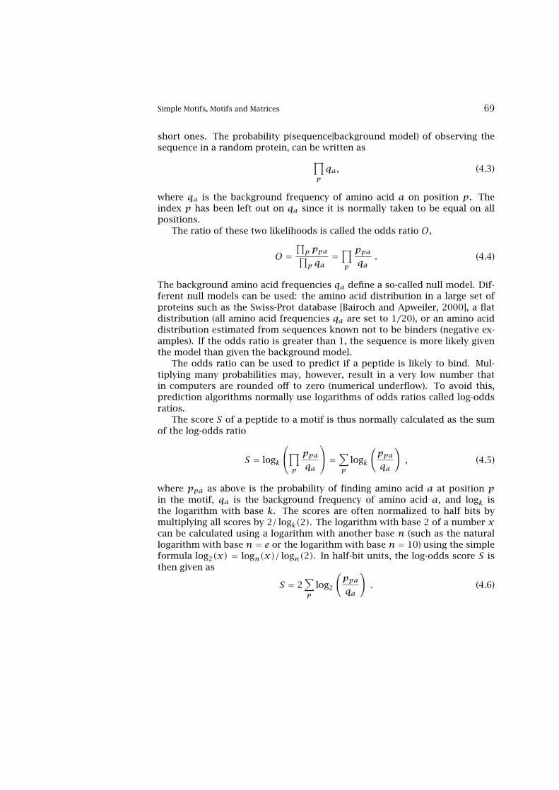
Simple Motifs, Motifs and Matrices 69
short ones. The probability p(sequence|background model) of observing thesequence in a random protein, can be written as∏
pqa, (4.3)
where qa is the background frequency of amino acid a on position p. Theindex p has been left out on qa since it is normally taken to be equal on allpositions.
The ratio of these two likelihoods is called the odds ratio O,
O =∏p ppa∏p qa
=∏p
ppaqa
. (4.4)
The background amino acid frequencies qa define a so-called null model. Dif-ferent null models can be used: the amino acid distribution in a large set ofproteins such as the Swiss-Prot database [Bairoch and Apweiler, 2000], a flatdistribution (all amino acid frequencies qa are set to 1/20), or an amino aciddistribution estimated from sequences known not to be binders (negative ex-amples). If the odds ratio is greater than 1, the sequence is more likely giventhe model than given the background model.
The odds ratio can be used to predict if a peptide is likely to bind. Mul-tiplying many probabilities may, however, result in a very low number thatin computers are rounded off to zero (numerical underflow). To avoid this,prediction algorithms normally use logarithms of odds ratios called log-oddsratios.
The score S of a peptide to a motif is thus normally calculated as the sumof the log-odds ratio
S = logk
∏p
ppaqa
=∑p
logk
(ppaqa
), (4.5)
where ppa as above is the probability of finding amino acid a at position pin the motif, qa is the background frequency of amino acid a, and logk isthe logarithm with base k. The scores are often normalized to half bits bymultiplying all scores by 2/ logk(2). The logarithm with base 2 of a number xcan be calculated using a logarithm with another base n (such as the naturallogarithm with base n = e or the logarithm with base n = 10) using the simpleformula log2(x) = logn(x)/ logn(2). In half-bit units, the log-odds score S isthen given as
S = 2∑p
log2
(ppaqa
). (4.6)

70 Methods Applied in Immunological Bioinformatics
4.2 Information Carried by Immunogenic Sequences
Once the binding motif has been described by a probability matrix ppa, a num-ber of different calculations can be carried out characterizing the motif.
4.2.1 Entropy
The entropy of a random variable is a measure of the uncertainty of the ran-dom variable; it is a measure of the amount of information required to describethe random variable [Cover and Thomas, 1991]. The entropy H (also called theShannon entropy) of an amino acid distribution p is defined as
H(p) = −∑apa log2(pa) , (4.7)
where pa is the probability of amino acid a. Here the logarithm used has thebase of 2 and the unit of the entropy then becomes bits [Shannon, 1948]. Theentropy attains its maximal value log2(20) ' 4.3 if all amino acids are equallyprobable, and becomes zero if only one amino acid is observed at a givenposition. We here use the definition that 0 log(0) = 0. For the data shown intable 4.1 the entropy at position 2 is, e.g., found to be ' 1.36.
4.2.2 Relative Entropy
The relative entropy can be seen as a distance between two probability distri-butions, and is used to measure how different an amino acid distribution p isfrom some background distribution q. The relative entropy is also called theKullback-Leibler distance D and is defined as
D(p‖q) =∑apa log2(
paqa) . (4.8)
The background distribution is often taken as the distribution of amino acidsin proteins in a large database of sequences. Alternatively, q and p can be thedistributions of amino acids among sites that are known to have or not havesome property. This property could, e.g., be glycosylation, phosphorylation,or MHC binding.
The relative entropy attains its maximal value if only the least probableamino acid according to the background distribution is observed. The relativeentropy is non-negative and becomes zero only if p = q. It is not a true metric,however, since it is not symmetric (D(p‖q) 6= D(q‖p)) and does not satisfy thetriangle inequality (D(p‖q) 6< D(p‖r)+D(r‖q)) [Cover and Thomas, 1991].

Information Carried by Immunogenic Sequences 71
4.2.3 Logo Visualization of Relative Entropy
To visualize the characteristics of binding motifs, the so-called sequence logotechnique [Schneider and Stephens, 1990] is often used. The information con-tent at each position in the sequence motif is indicated using the height of acolumn of letters, representing amino acids or nucleotides. For proteins theinformation content is normally defined as the relative entropy between theamino acid distribution in the motif, and a background distribution where allamino acids are equally probable. This gives the following relation for theinformation content:
I =∑apa log2
pa1/20
= log2(20)+∑apa log2 pa . (4.9)
The information content is a measure of the degree of conservation and has avalue between zero (no conservation; all amino acids are equally probable) andlog2(20) ' 4.3 (full conservation; only a single amino acid is observed at thatposition). In the logo plot, the height of each letter within a column is propor-tional to the frequency pa of the corresponding amino acid a at that position.When another background distribution is used, the logos are normally calledKullback-Leibler logos, and letters that are less frequent than the backgroundare displayed upside down.
In logo plots, the amino acids are normally colored according to their prop-erties:
• Acidic [DE]: red
• Basic [HKR]: blue
• Hydrophobic [ACFILMPVW]: black
• Neutral [GNQSTY]: green
But other color schemes can be used if relevant in a given context. An exampleof a logo can be seen in Figure 4.1.
4.2.4 Mutual Information
Another important quantity used for characterizing a motif is the mutual in-formation. This quantity is a measure of correlations between different po-sitions in a motif. The mutual information measure is in general defined asthe reduction of the uncertainty due to another random variable and is thusa measure of the amount of information one variable contains about another.Mutual information between two variables is defined as
I(A;B) =∑a
∑bpab log2(
pabpapb
) , (4.10)
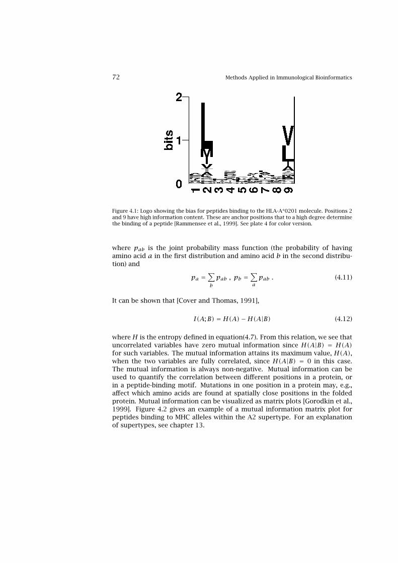
72 Methods Applied in Immunological Bioinformatics
Figure 4.1: Logo showing the bias for peptides binding to the HLA-A*0201 molecule. Positions 2and 9 have high information content. These are anchor positions that to a high degree determinethe binding of a peptide [Rammensee et al., 1999]. See plate 4 for color version.
where pab is the joint probability mass function (the probability of havingamino acid a in the first distribution and amino acid b in the second distribu-tion) and
pa =∑bpab , pb =
∑apab . (4.11)
It can be shown that [Cover and Thomas, 1991],
I(A;B) = H(A)−H(A|B) (4.12)
where H is the entropy defined in equation(4.7). From this relation, we see thatuncorrelated variables have zero mutual information since H(A|B) = H(A)for such variables. The mutual information attains its maximum value, H(A),when the two variables are fully correlated, since H(A|B) = 0 in this case.The mutual information is always non-negative. Mutual information can beused to quantify the correlation between different positions in a protein, orin a peptide-binding motif. Mutations in one position in a protein may, e.g.,affect which amino acids are found at spatially close positions in the foldedprotein. Mutual information can be visualized as matrix plots [Gorodkin et al.,1999]. Figure 4.2 gives an example of a mutual information matrix plot forpeptides binding to MHC alleles within the A2 supertype. For an explanationof supertypes, see chapter 13.

Sequence Weighting Methods 73
Figure 4.2: Mutual information plot calculated from peptides binding to MHC alleleswithin the A2 supertype. The plot was made using MatrixPlot [Gorodkin et al., 1999](http://www.cbs.dtu.dk/services/MatrixPlot/).
4.3 Sequence Weighting Methods
In the following, we will use the logo plots to visualize some problems oneoften faces when deriving a binding motif characterized by a probability matrixppa as described in section 4.1.
The values of ppa may be set to the frequencies fab observed in the align-ment. There are, however, some problems with this direct approach. In figure4.3, a logo representation of the probability matrix calculated from the pep-tides in table 4.1 is shown. From the plot, it is clear that alanine has a veryhigh probability at all positions in the binding motif. The first 5 sequences inthe alignment are very similar, and may reflect a sampling bias, rather than anactual amino acids bias in the binding motif. In such a situation, one wouldtherefore like to downweight identical or almost identical sequences.
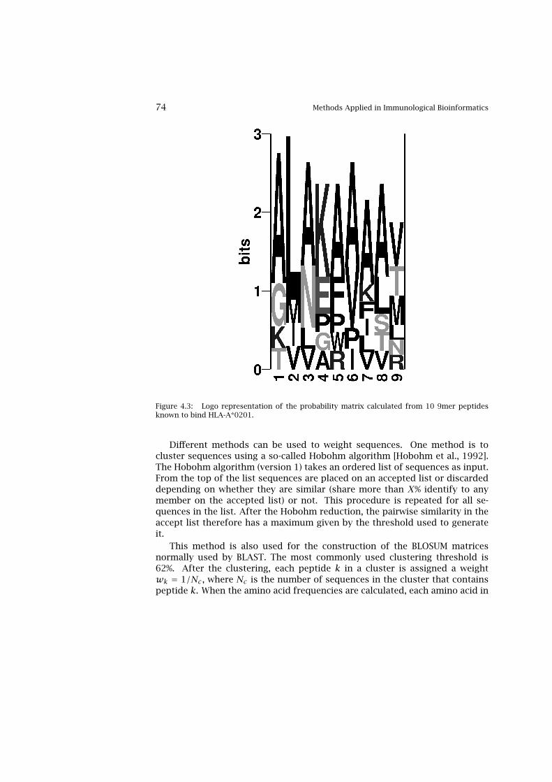
74 Methods Applied in Immunological Bioinformatics
Figure 4.3: Logo representation of the probability matrix calculated from 10 9mer peptidesknown to bind HLA-A*0201.
Different methods can be used to weight sequences. One method is tocluster sequences using a so-called Hobohm algorithm [Hobohm et al., 1992].The Hobohm algorithm (version 1) takes an ordered list of sequences as input.From the top of the list sequences are placed on an accepted list or discardeddepending on whether they are similar (share more than X% identify to anymember on the accepted list) or not. This procedure is repeated for all se-quences in the list. After the Hobohm reduction, the pairwise similarity in theaccept list therefore has a maximum given by the threshold used to generateit.
This method is also used for the construction of the BLOSUM matricesnormally used by BLAST. The most commonly used clustering threshold is62%. After the clustering, each peptide k in a cluster is assigned a weightwk = 1/Nc , where Nc is the number of sequences in the cluster that containspeptide k. When the amino acid frequencies are calculated, each amino acid in

Pseudocount Correction Methods 75
sequence k is weighted by wk. In the above example the first 5 peptides willform one cluster, and each of these sequences thus contributes with a weightof 1
5 to the probability matrix. The frequency of A at position p1 will thenbe p1A = 2/6 = 0.33 as opposed to 6/10 = 0.6 found when using the rawsequence counts.
In the Henikoff and Henikoff [1994] sequence weighting scheme, an aminoacid a on position p in sequence k contributes a weight wkp = 1/rs, where ris the number of different amino acids at a given position (column) in the align-ment and s the number of occurrences of amino acid a in that column. Theweight of a sequence is then assigned as the sum of the weights over all posi-tions in the alignment. The Henikoffs’ method is fast as the computation timeonly increases linearly with the number of sequences. For the Hobohm cluster-ing algorithm, on the other hand, computation time increases as the square ofthe number of sequences (depending on the similarity between the sequences).Performing the sequence weighting using clustering generally leads to more ac-curate results, and clustering is the suggested choice of method if the numberof sequences is limited and the calculation thus computationally feasible.
Figure 4.4 shows a logo representation of the probability matrix calculatedusing clustering sequence weighting. From the figure it is apparent that thestrong alanine bias in the motif has been removed.
4.4 Pseudocount Correction Methods
Another problem with the direct approach to estimating the probability matrixppa is that the statistics often will be based on very few sequence examples (inthis case 10 sequences). A direct calculation of the probability p9I for observ-ing an isoleucine on position 9 in the alignment, e.g., gives 0. This will in turnmean that all peptides with an isoleucine on position 9 will score minus infin-ity in equation (4.5), i.e., be predicted not to bind no matter what the rest of thesequence is. This may be too drastic a conclusion based on only 10 sequences.One solution to this problem is to use a pseudocount method, where priorknowledge about the frequency of different amino acids in proteins is used.Two strategies for pseudocount correction will be described here: Equal andBLOSUM correction, respectively. In both cases the pseudocount frequencygpa for amino acid a on position p in the alignment is estimated as describedby Altschul et al. [1997],
gpa =∑b
fpbqb
qab =∑bfpb qa|b . (4.13)
Here, fpb is the observed frequency of amino acid b on position p, qb is thebackground frequency of amino acid b, qab is the frequency by which amino

76 Methods Applied in Immunological Bioinformatics
Figure 4.4: Logo representation of the probability matrix calculated from 10 9mer peptidesknown to bind HLA-A*0201. The probabilities are calculated using the clustering sequenceweighting method.
acid a is aligned to amino acid b derived from the BLOSUM substitution matrix,and qa|b is the corresponding conditional probability. The equation shows howthe pseudo-count frequency can be calculated. The pseudocount frequency forisoleucine at position 9 in the example in table 4.1 would, e.g., be
g9I =∑bf9b qI|b = 0.3 qI|V + 0.2 qI|T . . .0.1 qI|L ' 0.09 , (4.14)
where here, for simplicity, we have used the raw count values for f9b. Inreal applications the sequence-weighted probabilities are normally used. Theqa|b values are taken from the BLOSUM62 substitution matrix [Henikoff andHenikoff, 1992].
In the Equal correction, a substitution matrix with identical frequencies forall amino acids (1/20) and all amino acid substitutions (1/400) is applied. Inthis case gpa = 1/20 at all positions for all amino acids.

Weight on Pseudocount Correction 77
4.5 Weight on Pseudocount Correction
From estimated pseudocounts, and sequence-weighted observed frequencies,the effective amino acid frequency can be calculated as [Altschul et al., 1997]
ppa =αfpa + βgpa
α+ β . (4.15)
Here fpa is the observed frequency (calculated using sequence weighting), gpathe pseudocount frequency, α the effective sequence number minus 1, andβ the weight on the pseudocount correction. When the sequence weightingis performed using clustering, the effective sequence number is equal to thenumber of clusters. When sequence weighting as described by Henikoff andHenikoff [1992] is applied, the average number of different amino acids in thealignment gives the effective sequence number. If a large number of differentsequences are available α will in general also be large and a relative low weightwill thus be put on the pseudocount frequencies. If, on the other hand, thenumber of observed sequences is one, α is zero, and the effective amino acidfrequency is reduced to the pseudocount frequency gpa. If we calculate thelog-odds score S, for a G, as given by equation (4.5), G gets the score:
SG = loggpGqG
= logqGGqGqG
, (4.16)
where we have used equation (4.13) for gpa. The last log-odds score is theBLOSUM matrix score for G−G, and we thus find that the log-odds score for asingle sequence reduces to the BLOSUM identical match score values.
Figure 4.5 shows the logo plot of the probability matrix calculated fromthe sequences in table 4.1, including sequence weighting and pseudocountcorrection. The figure demonstrates how the pseudocount correction allowsfor probability estimates for all 20 amino acids at all positions in the motif.Note that I is the fifth most probable amino acid at position 9, even thoughthis amino acid was never observed at the position in the peptide sequences.
4.6 Position Specific Weighting
In many situations prior knowledge about the importance of the different po-sitions in the binding motif exists. Such prior knowledge can with success beincluded in the search for binding motifs [Lundegaard et al., 2004, Rammenseeet al., 1997]. In figure 4.6, we show the results of such a position-specificweighting. The figure displays the probability matrix calculated from the 10sequences and a matrix calculated from a large set of 485 peptides. It demon-strates how a reasonably accurate motif description can be derived from a very

78 Methods Applied in Immunological Bioinformatics
Figure 4.5: Logo representation of the probability matrix calculated from 10 9mer peptidesknown to bind HLA-A*0201. The probabilities are calculated using both the methods of se-quence weighting and pseudocount correction.
limited set of data, using the techniques of sequence weighting, pseudocountcorrection, and position-specific weighting.
4.7 Gibbs Sampling
In previous sections, we have described how a weight matrix describing a se-quence motif can be calculated from a set of peptides of equal length. This ap-proach is appropriate when dealing with MHC class I binding, where the lengthof the binding peptides are relatively uniform. MHC class II molecules, on theother hand, can bind peptides of very different length, and the weight-matrixmethods described up to now are hence not directly applicable to characterizethis type of motif. Here we describe a motif sampler suited to deal with suchproblems.
The general problem to be solved by the motif sampler is to locate and
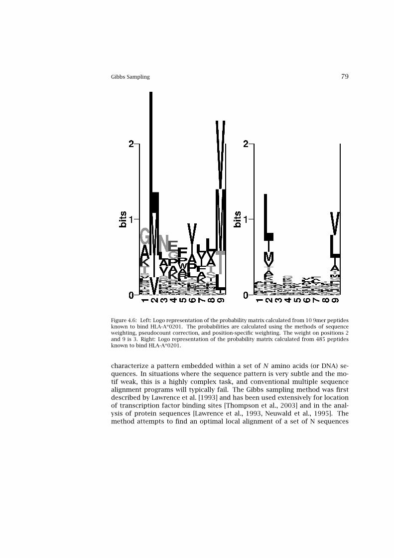
Gibbs Sampling 79
Figure 4.6: Left: Logo representation of the probability matrix calculated from 10 9mer peptidesknown to bind HLA-A*0201. The probabilities are calculated using the methods of sequenceweighting, pseudocount correction, and position-specific weighting. The weight on positions 2and 9 is 3. Right: Logo representation of the probability matrix calculated from 485 peptidesknown to bind HLA-A*0201.
characterize a pattern embedded within a set of N amino acids (or DNA) se-quences. In situations where the sequence pattern is very subtle and the mo-tif weak, this is a highly complex task, and conventional multiple sequencealignment programs will typically fail. The Gibbs sampling method was firstdescribed by Lawrence et al. [1993] and has been used extensively for locationof transcription factor binding sites [Thompson et al., 2003] and in the anal-ysis of protein sequences [Lawrence et al., 1993, Neuwald et al., 1995]. Themethod attempts to find an optimal local alignment of a set of N sequences

80 Methods Applied in Immunological Bioinformatics
by means of Metropolis Monte Carlo sampling [Metropolis et al., 1953] of thealignment space. The scoringfunction guiding the Monte Carlo search is de-fined in terms of fitness (information content) of a log-odds matrix calculatedfrom the alignment.
The algorithm samples possible alignments of the N sequences. For eachalignment a log-odds weight matrix is calculated as log(ppa/qa), where ppais the frequency of amino acid a at position p in the alignment and qa is thebackground frequency of that amino acid. The values of ppa can be estimatedusing sequence weighting and pseudocount correction for low counts as de-scribed earlier in this chapter.
The fitness (energy) of an alignment is calculated as
E =∑p,aCpa log
ppaqa
, (4.17)
where Cpa is the number of times amino acid a is observed at position p inthe alignment, ppa is the pseudocount and sequence weight corrected aminoacid frequency of amino acid b and position p in the alignment. Finally, qais the background frequency of amino acid a. E is equal to the sum of therelative entropy or the Kullback-Leibler distance [Kullback and Leibler, 1951]in the window.
The set of possible alignments is, even for a small data set, very large. Fora set of 50 peptides of length 10, the number of different alignments witha core window of nine amino acids is 250 ' 1015. This number is clearlytoo large to allow for a sampling of the complete alignment space. Instead,the Metropolis Monte Carlo algorithm is applied [Metropolis et al., 1953] toperform an effective sampling of the alignment space.
Two distinct Monte Carlo moves are implemented in the algorithm: (1) thesingle sequence move, and (2) the phase shift move. In the single sequencemove, the alignment of a sequence is shifted a randomly selected number ofpositions. In the phase shift move, the window in the alignment is shifted arandomly selected number of residues to the left or right. This latter type ofmove allows the program to efficiently escape local minima. This may, e.g.,occur if the window overlaps the most informative motif, but is not centeredon the most informative pattern.
The probability of accepting a move in the Monte Carlo sampling is definedas
P = min(1, edE/T ) , (4.18)
where dE is difference in (fitness) energy between the end and start configu-rations and T is a scalar. Note that we seek to maximize the energy function,hence the positive sign for dE in the equation. T is a scalar that is loweredduring the calculation. The equation implies that moves that increase E will

Gibbs Sampling 81
Figure 4.7: Example of an alignment generated by the Gibbs sampler for the DR4(B1*0401)binding motif. The peptides were downloaded from the MHCPEP database [Brusic et al., 1998a].Top left: Unaligned sequences. Top right: Logo for unaligned sequences. Bottom left: Sequencesaligned by Gibbs sampler. Bottom right: Logo for sequences aligned by the Gibbs sampler.Reprinted, with permission, from Nielsen et al. [2004]. See plate 5 for color version.
always be accepted (dE > 0). On the other hand, only a fraction given byedE/T of the moves which decrease E will be accepted. For high values of thescalar T (T � dE) this probability is close to 1, but as T is lowered during thecalculation, the probability of accepting unfavorable moves will be reduced,forcing the system into a state of high fitness (energy). Figure 4.7 shows a setof sequences aligned by their N-terminal (top left) and the corresponding logo(top right). The lower panel shows the alignment by the Gibbs sampler and thecorresponding logo. The figure shows how the Gibbs sampler has identified amotif describing the binding to the DR4(B1*0401) allele. For more details onthe Gibbs sampler see Chapter 8.

82 Methods Applied in Immunological Bioinformatics
4.8 Hidden Markov Models
The Gibbs sampler and other weight-matrix approaches are well suited to de-scribe sequence motifs of fixed length. For MHC class II, the peptide bindingmotif is in most situations assumed to be of a fixed length of 9 amino acids.This implies that the scoringfunction for a peptide binding to the MHC com-plex can be written as a linear sum of 9 terms. In many situations this simplemotif description is, however, not valid. In the previous chapter, we describedhow protein families, e.g, often are characterized by conserved amino acid re-gions separated by amino acid segments of variable length. In such situationsa weight matrix approach is poorly suited to characterize the motif. HMMs, onthe other hand, provide a natural framework for describing such interruptedmotifs.
In this section, we will give a brief introduction to the HMM framework.First, we describe the general concepts of the HMM framework through a sim-ple example. Next the Viterbi and posterior decoding algorithms for aligninga sequence to a HMM are explained, and finally the use of HMMs in some se-lected biological problems is described. A detailed introduction to HMMs andtheir application to sequence analysis problems may be found, e.g., in Durbinet al. [1998] and Baldi and Brunak [2001].
4.8.1 Markov Model, Markov Chain
A Markov model consists of a set of states. Each state is associated with aprobability distribution assigning probability values to the set of possible out-comes. A set of transition probabilities for switching between the states isassigned. In a Markov model (or Markov chain) the outcome of an event de-pends only on the preceding state.
An example of such a model is a B cell epitope model. Regions in thesequence with many hydrophobic residues are less likely to be exposed onthe surface of proteins and it is therefore less likely that antibodies can bindto these regions. In this model, we divide positions in a protein in two states:epitopes E and non-epitopes N. We divide the 20 different amino acids in threegroups. Hydrophobic [ACFILMPVW] , uncharged polar [GNQSTY] and charged[DEHKR]. This model is displayed in Figure 4.8. Even though this model ishighly simplified and does only capture the most simple, of the very complex,features describing the B cell epitopes, it serves the purpose of introducingthe important concepts of an HMM.
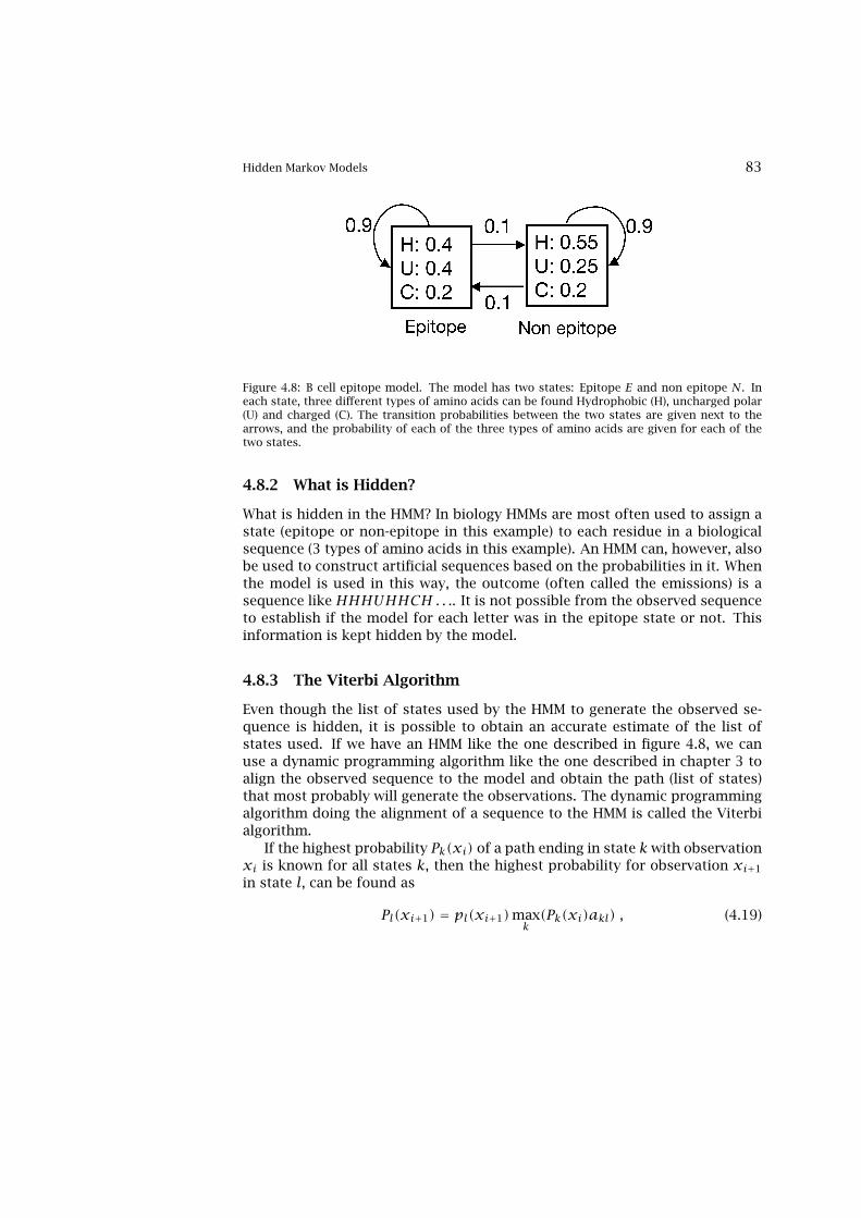
Hidden Markov Models 83
Figure 4.8: B cell epitope model. The model has two states: Epitope E and non epitope N. Ineach state, three different types of amino acids can be found Hydrophobic (H), uncharged polar(U) and charged (C). The transition probabilities between the two states are given next to thearrows, and the probability of each of the three types of amino acids are given for each of thetwo states.
4.8.2 What is Hidden?
What is hidden in the HMM? In biology HMMs are most often used to assign astate (epitope or non-epitope in this example) to each residue in a biologicalsequence (3 types of amino acids in this example). An HMM can, however, alsobe used to construct artificial sequences based on the probabilities in it. Whenthe model is used in this way, the outcome (often called the emissions) is asequence like HHHUHHCH . . .. It is not possible from the observed sequenceto establish if the model for each letter was in the epitope state or not. Thisinformation is kept hidden by the model.
4.8.3 The Viterbi Algorithm
Even though the list of states used by the HMM to generate the observed se-quence is hidden, it is possible to obtain an accurate estimate of the list ofstates used. If we have an HMM like the one described in figure 4.8, we canuse a dynamic programming algorithm like the one described in chapter 3 toalign the observed sequence to the model and obtain the path (list of states)that most probably will generate the observations. The dynamic programmingalgorithm doing the alignment of a sequence to the HMM is called the Viterbialgorithm.
If the highest probability Pk(xi) of a path ending in state k with observationxi is known for all states k, then the highest probability for observation xi+1
in state l, can be found as
Pl(xi+1) = pl(xi+1)maxk(Pk(xi)akl) , (4.19)

84 Methods Applied in Immunological Bioinformatics
where pl(xi+1) is the probability of observation xi+1 in state l, and akl is thetransition probability from state k to state l.
By using this relation recursively, one can find the path through the modelthat most probably will give the observed sequence. To avoid underflow inthe computer the algorithm normally will work in log-space and calculatelogPl(xi+1) instead. In log-space the recursive equation becomes a sum, andthe numbers remain within a reasonable range.
An example of how the Viterbi algorithm is applied is given in figure 4.9.The figure shows how the optimal path through the HMM of figure 4.8 iscalculated for a sequence of NGSLFWIA. By translating the sequence intothe three states defining hydrophobic, neutral and charged residues, we getHHHUUUUU . In the example, we assume that the model is the non-epitopestate at the first H, which implies that is PE(H1) = −∞. The value for assign-ing H to the state N is PN(H1) = log(0.55) = −0.26. For the next residue, thepath must come from the N state. We therefore find, PN(H2) = log(0.55) +log(0.9) − 0.26 = −0.57, and PE(H2) = log(0.4) + log(0.1) − 0.26 = −1.66,since aNN0.9, and aNE = 0.1. The backtracking arrows are for both the E andthe N state placed to the previous N state. For the third residue the path tothe N state can come from both the N and the E states. The value PN(H3) istherefore found using the relation
PN(H3) = log(0.55)+max{log(0.9)− 0.57, log(0.1)− 1.66} = −0.88 (4.20)
and likewise the value PE(H3) is
PE(H3) = log(0.4)+max{log(0.1)− 0.57, log(0.9)− 1.66} = −1.97 (4.21)
In both cases the max function selects the first argument, and the backtrackingarrows are therefore for both the E and the N state assigned to the previousN state. This procedure is repeated for all residues in the sequence, and weobtain the result shown in Figure 4.9. With the arrows, it is indicated whichstate was selected in the maxk function in each step in the recursive calcula-tion. Repeating the calculation for all residues in the observed sequence, wefind that the highest score −4.08 is found in state E. Backtracking throughthe arrows, we find the optimal path to be EEENNNNN (indicated with solidarrows). Note that the most probable path of the sequence HHHUUUU wouldhave ended in the state N with a value of −3.48, and the corresponding pathwould hence have been NNNNNNN. Observing a series of uncharged aminoacids thus does not necessarily mean that the epitope state was used.
4.8.4 The Forward-Backward Algorithm and Posterior Decoding
Many different paths through an HMM can give rise to the same observed se-quence. Where the Viterbi algorithm gives the most probable path through an

Hidden Markov Models 85
Figure 4.9: Alignment of sequence HHHUUUUU to the B cell epitope model of figure 4.8. Theupper part of the figure shows the log-transformed HMM. The probabilities have been trans-formed by taking the logarithm with base 10. The model is assumed to start in the non-epitopestate at the first H. The table in the lower part gives the logPl(xi+1) values for the differentobservations in the N (non epitope), and E (epitope) states, respectively. The arrows show thebacktracking pointers. The solid arrows give the optimal path, the dotted arrows denote thesuboptimal path. The upper two rows in the table give the amino acid and three letter trans-formed sequence, respectively . The lower row gives the most probable path found using theViterbi algorithm.
HMM given the observed sequence, the so-called forward algorithm calculatesthe probability of the observed sequence being aligned to the HMM. This isdone by summing over all possible paths generating the observed sequence.The forward algorithm is a dynamic programming algorithm with a recursiveformula very similar to the Viterbi equation, replacing the maximization stepwith a sum [Durbin et al., 1998]. If fk(xi−1) is the probability of observing thesequence up to and including xi−1 ending in state k, then the probability ofobserving the sequence up to and including xi ending in state l can be foundusing the recursive formula
fl(xi) = pl(xi)∑kfk(xi−1)akl . (4.22)
Here pl(xi) is the probability of observation xi in state l, and akl is the transi-tion probability from state k to state l.
86 Methods Applied in Immunological Bioinformatics
Another important algorithm is the posterior decoding or forward-backward algorithm. The algorithm calculates the probability that an ob-servation xi is aligned to the state k given the observed sequence x. Theterm “posterior decoding” refers to the fact that the decoding is done af-ter the sequence is observed. This probability can formally be written asP(πi = k|x) and can be determined using the so-called forward-backwardalgorithm [Durbin et al., 1998].
P(πi = k|x) =fk(i)bk(i)P(x)
. (4.23)
The term fk(i) is calculated using the forward recursive formula from before,
fk(i) = pk(xi)∑lfl(xi−1)alk , (4.24)
and bk(i) is calculated using a backward recursive formula,
bk(xi) =∑laklpl(xi+1)bl(i+ 1) . (4.25)
From these relations, we see why the algorithm is called forward-backward.fk(i) is the probability of aligning the sequence up to and including xi witha path ending in state k, and bk(i) is the probability of aligning the sequencexi+1 . . . xN to the HMM starting from state k. Finally P(x) is the probability ofaligning the observed sequence to the HMM.
One of the most important applications of the forward-backward algorithmis the posterior decoding. Often many paths through the HMM will have prob-abilities very close to the optimal path found by the Viterbi algorithm. In suchsituations posterior decoding might be a more adequate algorithm to extractproperties of the observed sequence from the model. Posterior decoding givesa list of states that most probably generate the observed sequence using theequation
πposteriori = maxkP(πi = k|x) , (4.26)
where P(πi = k|x) is the probability of observation xi being aligned to stateπk given the observed sequence x. Note that posterior decoding is differentfrom the Viterbi decoding since the list of states found by posterior decodingneed not be a legitimate path through the HMM.
4.8.5 Higher Order Hidden Markov Models
The central property of the Markov chains described until now is the fact thatthe probability of an observation only depends on the previous state and that

Hidden Markov Models 87
the probability of an observed sequence, X, thus can be written as
P(X) = P(x1)P(x2|x1)P(x3|x2) · · ·P(xN|xN−1) (4.27)
where P(xi) denotes the probability of observing x at position i.In many situations, this approximation might not be valid since the proba-
bility of an observation might depend on more than just the preceding state.However by use of higher order Markov models, such dependences can be cap-tured. In a Markov model of n’th order, the probability of an observation xi isgiven by
P(xi) = P(xi|xi−1, . . . , xi−n) (4.28)
A second order hidden Markov model describing B cell epitopes may thusconsist of two states each with 9 possible observations HH, HU , HC , UH,UU , UC , CH, CU , and CC . By assigning different probability values to forinstance the observationsHU , UU and CU , the model can capture higher ordercorrelations.
An n’th order Markov model over some alphabet is thus equivalent to a firstorder Markov chain over an alphabet of n-tuples.
4.8.6 Hidden Markov Models in Immunology
Having introduced the HMM framework through a simple example, we nowturn to some relevant biological problems that are well described using HMMs.The first is highly relevant to antigen processing, and describes how anHMM can be designed to characterize the binding of peptides to the humantransporter associated with antigen processing (TAP). The second exampleaddresses a more general use of HMMs in characterizing similarities betweenprotein sequences, the so-called profile HMMs.
TAP Transport of the peptides into the endoplasmic reticulum is an essen-tial step in the MHC class I presentation pathway. This task is done by TAPmolecules and a detailed description of the function of the TAP molecules isgiven in chapter 7. The peptides binding to TAP have a rather broad length dis-tribution, and peptides up to a length of 18 amino acids can be translocated[van Endert et al., 1994]. The binding of a peptide to the TAP molecules is toa high degree determined by the first three N-terminal positions and the lastC-terminal position in the peptide. Other positions in the peptide determinethe binding to a lesser degree. The binding of a peptide to the TAP moleculesis thus an example of a problem where the binding motif has variable length,and hence a problem that is well described by a HMM. Figure 4.10 shows anHMM describing peptide TAP binding. The figure highlights the importantdifferences and similarities between a weight matrix and an HMM. If we only

88 Methods Applied in Immunological Bioinformatics
Figure 4.10: HMM for peptide TAP binding. The model can describe binding of peptides ofdifferent lengths to the TAP molecules. The binding motif consists of 9 amino acids. The firstthree N-terminal amino acids, and the last C-terminal amino acids must be part of the bindingmotif. Each state is associated with a probability distribution of matching one of the 20 aminoacids. The arrow between the states indicates the transition probabilities for switching betweenthe states. The amino acid probability distributions for each state are estimated using thetechniques of sequence weighting and pseudocount correction (see section 4.4).
consider alignment of 9mer peptides to the HMM, we see that no alignmentcan go through the insertion states (labeled as I in the figure). In this situationthe alignment becomes a simple sum of the amino acid match scores fromeach of the 9 states N1-N3, P1-P5, and C9, and the HMM is reduced to a sim-ple weight matrix. However, if the peptide is longer than nine amino acids,the path through the HMM must pass some insertion state, and it is clear thatsuch a motif could not have been characterized well by a weight matrix.
Profile Hidden Markov Models Profile HMMs are used to characterize se-quence similarities within a family of proteins. As described in chapter 3 amultiple alignment of protein sequences within a protein family can reveal im-portant information about amino acids conservation, mutability, active sites,etc.
A profile HMM provides a natural framework for compiling such informa-tion of a multiple alignment. In figure 4.11, we show an example of a profileHMM. The architecture of a profile HMM is very similar to the model for pep-tide TAP binding. The model is build from a set of match states (P1-P7). Thesestates describe what is conserved among most sequences in the protein fam-ily. Some sequences within a family will have amino acid insertions; others willhave amino acid deletions with respect to the motif. To allow for such varia-tion in sequence, the profile HMM has insertion and deletion states (labeled asI and D in the figure, respectively). The model can insert amino acids betweenmatch states using the insertion state, and a match state can be skipped usingthe deletion states.
An example of a multiple alignment was given in figure 3.12C. From thistype of alignment, one can construct a profile HMM. If we consider positions
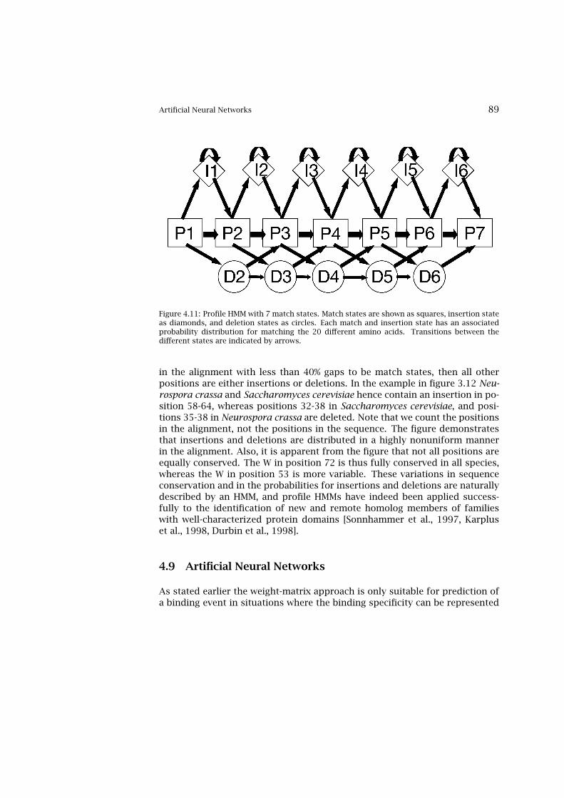
Artificial Neural Networks 89
Figure 4.11: Profile HMM with 7 match states. Match states are shown as squares, insertion stateas diamonds, and deletion states as circles. Each match and insertion state has an associatedprobability distribution for matching the 20 different amino acids. Transitions between thedifferent states are indicated by arrows.
in the alignment with less than 40% gaps to be match states, then all otherpositions are either insertions or deletions. In the example in figure 3.12 Neu-rospora crassa and Saccharomyces cerevisiae hence contain an insertion in po-sition 58-64, whereas positions 32-38 in Saccharomyces cerevisiae, and posi-tions 35-38 in Neurospora crassa are deleted. Note that we count the positionsin the alignment, not the positions in the sequence. The figure demonstratesthat insertions and deletions are distributed in a highly nonuniform mannerin the alignment. Also, it is apparent from the figure that not all positions areequally conserved. The W in position 72 is thus fully conserved in all species,whereas the W in position 53 is more variable. These variations in sequenceconservation and in the probabilities for insertions and deletions are naturallydescribed by an HMM, and profile HMMs have indeed been applied success-fully to the identification of new and remote homolog members of familieswith well-characterized protein domains [Sonnhammer et al., 1997, Karpluset al., 1998, Durbin et al., 1998].
4.9 Artificial Neural Networks
As stated earlier the weight-matrix approach is only suitable for prediction ofa binding event in situations where the binding specificity can be represented
90 Methods Applied in Immunological Bioinformatics
independently at each position in the motif. In many (in fact most) situationsthis is not the case, and this assumption can only be considered to be an ap-proximation. In the binding of a peptide to the MHC molecule the amino acidsmight, e.g., compete for the space available in the binding grove. The mutualinformation in the binding motif will allow for identification of such higher-order sequence correlations. An example of a mutual information calculationfor peptides binding to the MHC class I complex is shown in figure 4.2.
Neural networks with a hidden layer are designed to describe sequencepatterns with such higher-order correlations. Due to their ability to handlethese correlations, hundreds of different applications within bioinformaticshave been developed using this technique, and for that reason ANNs havebeen enjoying a renaissance, not only in biology but also in many other datadomains.
Neural networks realize a method of computation that is vastly differentfrom “rule-based techniques” with strict control over the steps in the calcula-tion from data input to output. Conceptually, neural networks, on the otherhand, use “influence” rather than control. A neural network consists of a largenumber of independent computational units that can influence but not con-trol each other’s computations. That such a system, which consists of a largenumber of unintelligent units, in their biological counterparts can be made toexhibit “intelligent” behavior is not directly obvious, but one can with somejustification use the central nervous system in support of the idea. However,the ANNs obviously do not to any extent match the computing power and so-phistication of biological neural systems.
ANNs are not programmed in the normal sense, but must be influenced bydata — trained — to associate patterns with each other.
The neural network algorithm most often used in bioinformatics is similarto the network structure described by Rumelhart et al. [1991]. This networkarchitecture is normally called a standard, feedforward multilayer perceptron.Other neural network architectures have also been used, but will not be de-scribed here. The most successful of the more complex networks involves dif-ferent kinds of feedback, such that the network calculation on a given (oftenquite short) amino acid sequence segment possibly can depend on sequencepatterns present elsewhere in the sequence. When analyzing nucleotide datathe applications have typically been used also for long sequence segments,such as the determination of whether a given nucleotide belongs to a proteincoding sequence or not. The network can in such a case be trained to takeadvantage of long-range correlations hundreds of nucleotide positions apartin a sequence.
The presentation of the neural network theory outlined below is based onthe paper by Rumelhart et al. [1991], as well as the book by Hertz et al. [1991].The training algorithm used to produce the final network is a steepest descent

Artificial Neural Networks 91
method that learns a training set of input-output pairs by adjusting the net-work weight parameters such that the network for each input will produce anumerical value that is close to the desired target output (either representingdisjunct categories, or real values such as peptide binding affinities). The ideawith the network is to produce algorithms which can handle sequence corre-lations, and also classify data in a nonlinear manner, such that small changesin sequence input can produce large changes in output. The hope is that thenetwork then will be able to reproduce what is well-known in biology, namelythat many single amino acid substitutions can entirely disrupt a mechanism,e.g., by inhibiting binding.
The feedforward neural network consists of connected computing units.Each unit “observes” the other units’ activity through its input connections.To each input connection, the unit attaches a weight, which is a real numberthat indicates how much influence the input in question is to have on thatparticular unit. The influence is calculated as the weight multiplied by theactivity of the neuron delivering the input. The weight can be negative, so aninput can have a negative influence. The neuron sums up all the influence itreceives from the other neurons and thereby achieves a measure for the totalinfluence it is subjected to. From this sum the neuron subtracts a thresholdvalue, which will be omitted from the description below, since it can be viewedas a weight from an extra input unit, with a fixed input value of −1. The linearsum of the inputs is then transformed through a nonlinear, sigmoidal functionto produce its output. The input layer units does not compute anything, butmerely store the network inputs; the information processing in the networktakes place in the internal, hidden layer (most often only one layer), and inthe output layer. A schematic representation of this type of neural network isshown in figure 4.12.
4.9.1 Predicting Using Neural Networks: Conversion of Input to Out-put
Formally the calculation in a network with one hidden layer proceeds as fol-lows. Let the indices i, j, and k refer to the output, hidden, and input layers,respectively. The input neurons each receive an input Ik. The input to each ofthe hidden units is
hj =∑kvjkIk, (4.29)
where vjk is the weight on the input k to the hidden unit j. The output fromthe hidden units is
Hj = g(hj) (4.30)

92 Methods Applied in Immunological Bioinformatics
Figure 4.12: Schematic representation of a conventional feedforward neural network used innumerous applications within bioinformatics.
where
g(x) = 11+ e−x (4.31)
is the sigmoidal function most often used. Note that
g′(x) = g(x)(1− g(x)) . (4.32)
Each output neuron receives the input
oi =∑jwijHj , (4.33)
wherewij are the weights between the hidden and the output units to producethe final output
Oi = g(oi) . (4.34)
Different measures of the error between the network output and the de-sired target output can be used [Hertz et al., 1991, Bishop, 1995]. The mostsimple choice is to let the error E be proportional to the sum of the squareddifference between the desired output di and the output Oi from the last layerof neurons:
E = 12
∑i(Oi − di)2 . (4.35)
4.9.2 Training the Network by Backpropagation
One option is to update the weights by a back-propagation algorithm whichis a steepest descent method, where each weight is changed in the opposite
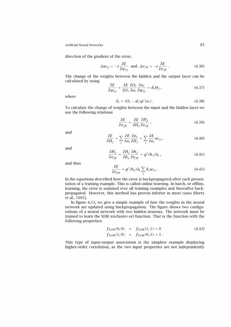
Artificial Neural Networks 93
direction of the gradient of the error,
∆wij = −ε∂E∂wij
and ∆vjk = −ε∂E∂vjk
. (4.36)
The change of the weights between the hidden and the output layer can becalculated by using
∂E∂wij
= ∂E∂Oi
∂Oi∂oi
∂oi∂wij
= δiHj , (4.37)
whereδi = (Oi − di)g′(oi) . (4.38)
To calculate the change of weights between the input and the hidden layer weuse the following relations
∂E∂vjk
= ∂E∂Hj
∂Hj∂vjk
, (4.39)
and∂E∂Hj
=∑i
∂E∂oi
∂oi∂Hj
=∑i
∂E∂oi
wij , (4.40)
and∂Hj∂vjk
= ∂Hj∂hj
∂hj∂vjk
= g′(hj)Ik , (4.41)
and thus∂E∂vjk
= g′(hj)Ik∑iδiwij . (4.42)
In the equations described here the error is backpropagated after each presen-tation of a training example. This is called online learning. In batch, or offline,learning, the error is summed over all training examples and thereafter back-propagated. However, this method has proven inferior in most cases [Hertzet al., 1991].
In figure 4.13, we give a simple example of how the weights in the neuralnetwork are updated using backpropagation. The figure shows two configu-rations of a neural network with two hidden neurons. The network must betrained to learn the XOR (exclusive or) function. That is the function with thefollowing properties:
fXOR(0,0) = fXOR(1,1) = 0 (4.43)
fXOR(1,0) = fXOR(0,1) = 1 .
This type of input-output association is the simplest example displayinghigher-order correlation, as the two input properties are not independently

94 Methods Applied in Immunological Bioinformatics
Figure 4.13: Update of weights in a neural network using backpropagation. The figure showsthe neural network before updating the weights (left) and the network configuration after oneround of backpropagation (right). The learning rate ε in the example is equal to 0.5. Note thatthis is a large value for ε. Normally the value is of the order 0.05.
linked to the categories. The “1” category is represented by input exampleswhere only one of the two features are allowed to be present — not bothfeatures simultaneously. The (1,1) example from the “0” category is thereforean “exception,” and this small data set can therefore not be handled by alinear network without hidden units. The example may seem very simple;still it captures the essence of the sequence properties in many binding sites,where the two features could be charge and side chain volume, respectively.In actual application the number of input features is typically much higher.
In the example shown in figure 4.13, we have for simplicity left out thethreshold value normally subtracted from the input to each neuron. The fig-ure shows the neural network before updating the weights and the networkconfiguration after one round of backpropagation. With the example (1,1),the network output, O, from the network with the initial weights is 0.6. Thisgives the following relation for δ:
δ = (0.6− 0)g′(o) = 0.6 ·O · (1−O) = 0.15 , (4.44)
where we have used equation (4.32) for g′(o).The change of the weights from the hidden layer to the output neuron are
updated using equation (4.37):
∆w1 = −ε 0.15 · 0.5 = −0.075ε

Artificial Neural Networks 95
∆w2 = −ε 0.15 · 0.88 = −0.13ε . (4.45)
The change of the weights in the first layer are updated using equation (4.42)
∆v11 = −ε g′(h1) · 1 · δ · (−1)= ε H1 (1−H1) · δ= 0.04ε
∆v21 = −ε g′(h1) · 1 · δ · (−1) = 0.04ε (4.46)
∆v12 = −ε g′(h2) · 1 · δ · 1 = −0.02ε∆v22 = −ε g′(h2) · 1 · δ · 1 = −0.02ε .
Modifying the weights according to these values, we obtain the neural networkconfiguration shown to the right of figure 4.13. The network output from theupdated network is 0.57. Note that the error indeed has decreased. When thenetwork is trained on all four patterns of the XOR function during a numberof training cycles (including the three threshold weights), the network will inmost cases reach an optimal configuration, where the error on all four patternsis practically zero.
Figure 4.14 demonstrates how the XOR function is learned by the neuralnetwork. If we construct a neural network without a hidden layer this data setcannot be learned, whereas a network with two hidden neurons learns the fourexamples perfectly.
When examining the weight configuration of the fully trained network itbecomes clear how the data set from the XOR function has been learned bythe network. The XOR function can be written as
fXOR(x1, x2) = (x1 + x2)− 2x1x2 = y − z , (4.47)
where y = x1 + x2 and z = 2x1x2. From this relation, we see that the hiddenlayer allows the network to linearize the problem into a sum of two terms.The two functions y and z are encoded by the network using the properties ofthe sigmoid function. If we assume for simplicity that the sigmoid function isreplaced by a step function that emits the value 1 if the input value is greaterthan or equal to the threshold value and zero otherwise, then the y and zfunctions can be encoded having the weights vij = 1 for all values of i andj and the corresponding threshold values 1 and 2 for the first and secondhidden neuron, respectively. With these values for the weights and thresholds,the first hidden neuron will emit a value of 1 if either of the input values are1, and zero otherwise. The second hidden neuron will emit a value of 1 onlyif both the input neurons are 1. Setting the weights w1 = 1, and w2 = −1, thenetwork is now able to encode the XOR function.

96 Methods Applied in Immunological Bioinformatics
Figure 4.14: Neural network learning curves for nonlinear patterns. The plot shows the Pearsoncorrelation as a function of the number of learning cycles during neural network training. Theblack curve shows the learning curve for the XOR function for a neural network without hiddenneurons, and the gray curve shows the learning curve for the neural network with two hiddenneurons.
4.9.3 Sequence Encoding
To feed the neural network with sequence data the amino acids must be trans-formed into numerical values in the input layer. A large set of different encod-ing schemes exists. The most conventionally used is the sparse or orthogonalencoding scheme, where each amino acid is represented as a 20- or 21-bit bi-nary string. Alanine is represented as 10000000000000000000 and cysteine as01000000000000000000, · · ·, where the last digit is used to represent blank,N- and C-terminal positions in a sequence window, i.e., when a window extendsone of the ends of the sequence. Other encoding schemes take advantage ofthe physical and chemical similarities between the different amino acids. Onesuch encoding scheme is the BLOSUM encoding, where each amino acid is en-coded as the 20 BLOSUM matrix values for replacing the amino acid [Nielsenet al., 2003]. A summary of other sequence encoding schemes can be found in[Baldi and Brunak, 2001].
Performance Measures for Prediction Methods 97
Predicted positive Predicted negative TotalActual positive TP FN APActual negative FP TN ANTotal PP PN N
Table 4.2: Classification of predictions. TP: true positives (predicted positive, actual positive);TN: true negatives (predicted negative, actual negative); FP: false positives (predicted positive,actual negative); FN: false negatives (predicted negative, actual positive).
4.10 Performance Measures for Prediction Methods
A number of different measures are commonly used to evaluate the perfor-mance of predictive algorithms. These measures differ according to whetherthe performance of a real-valued predictor (e.g., binding affinities) or a classi-fication is to be evaluated.
In almost all cases percentages of correctly predicted examples are not thebest indicators of the predictive performance in classification tasks, becausethe number of positives often is much smaller than the number of negatives inindependent test sets. Algorithms that underpredict a lot will therefore appearto have a high success rate, but will not be very useful.
We define a set of performance measures from a set of data with N pre-dicted values pi and N actual (or target) values ai. The value pi is found usinga prediction method of choice, and the ai is the known corresponding targetvalue. By introducing a threshold ta, the N points can be divided into actualpositives AP (points with actual values ai greater than ta) and actual nega-tives AN . Similarly, by introducing a threshold for the predicted values tp, thepoints can be divided into predicted positives PP and predicted negatives PN .These definitions are summarized in table 4.2 and will in the following be usedto define a series of different performance measures.
4.10.1 Linear Correlation Coefficient
The linear correlation coefficient, which is also called Pearson’s r , or just thecorrelation coefficient, is the most widely used measure of the association be-tween pairs of values [Press et al., 1992]. It is calculated as
c =∑i(ai − a)(pi − p)√∑
i(ai − a)2√∑
i(pi − p)2, (4.48)
where the overlined letters denote average values. This is one of the bestmeasures of association, but as the name indicates it works best if the actual

98 Methods Applied in Immunological Bioinformatics
and predicted values when plotted against each other fall roughly on a line. Avalue of 1 corresponds to a perfect correlation and a value of −1 to a perfectanticorrelation (when the prediction is high, the actual value is low). A valueof 0 corresponds to a random prediction.
4.10.2 Matthews Correlation Coefficient
I f all the predicted and actual values only take one of two values (normally0 and 1) the linear correlation coefficient reduces to the Matthews correlationcoefficient [Matthews, 1975]
c = TPTN − FPFN√(TP + FN)(TN + FP)(TP + FP)(TN + FN)
= TPTN − FPFN√APANPPPN
. (4.49)
As for the Pearson correlation, a value of 1 corresponds to a perfect correla-tion.
4.10.3 Sensitivity, Specificity
Four commonly used measures are calculated by dividing the true posi-tives and negatives by the actual and predicted positives and negatives[Guggenmoos-Holzmann and van Houwelingen, 2000],
Sensitivity Sensitivity measures the fraction of the actual positives which arecorrectly predicted: sens = TP
AP .
Specificity Specificity denotes the fraction of the actual negatives which arecorrectly predicted: spec = TN
AN
PPV The positive predictive value (PPV) is the fraction of the predicted posi-tives which are correct: PPV = TP
PP .
NPV The negative predictive value (NPV) stands for the fraction of the negativepredictions which are correct: NPV = TN
PN .
4.10.4 Receiver Operator Characteristics Curves
One problem with the above measures (except Pearson’s r ) is that a thresh-old tp must be chosen to distinguish between predicted positives and neg-atives. When comparing two different prediction methods, one may have abetter Matthews correlation coefficient than the other. Alternatively, one mayhave a higher sensitivity or a higher specificity. Such differences may be dueto the choice of thresholds and in that case the two prediction methods may
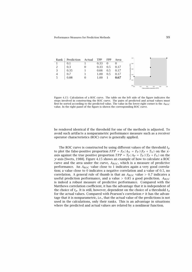
Performance Measures for Prediction Methods 99
Rank Prediction Actual TPP FPP Area1 0.1 1 0.33 0 02 0.3 0 0.33 0.5 0.173 0.35 1 0.66 0.5 0.174 0.7 1 1.00 0.5 0.175 0.88 0 1.00 1 0.67
0.0 0.2 0.4 0.6 0.8 1.0False positive proportion (FPP)
0.0
0.2
0.4
0.6
0.8
1.0
Tru
e po
sitiv
e pr
opor
tion
(TP
P)
Figure 4.15: Calculation of a ROC curve. The table on the left side of the figure indicates thesteps involved in constructing the ROC curve. The pairs of predicted and actual values mustfirst be sorted according to the predicted value. The value in the lower right corner is the AROCvalue. In the right panel of the figure is shown the corresponding ROC curve.
be rendered identical if the threshold for one of the methods is adjusted. Toavoid such artifacts a nonparametric performance measure such as a receiveroperator characteristics (ROC) curve is generally applied.
The ROC curve is constructed by using different values of the threshold tpto plot the false-positive proportion FPP = FP/AN = FP/(FP + TN) on the x-axis against the true positive proportion TPP = TP/AP = TP/(TP + FN) on they-axis [Swets, 1988]. Figure 4.15 shows an example of how to calculate a ROCcurve and the area under the curve, AROC , which is a measure of predictiveperformance. An AROC value close to 1 indicates again a very good correla-tion; a value close to 0 indicates a negative correlation and a value of 0.5, nocorrelation. A general rule of thumb is that an AROC value > 0.7 indicates auseful prediction performance, and a value > 0.85 a good prediction. AROCis indeed a robust measure of predictive performance. Compared with theMatthews correlation coefficient, it has the advantage that it is independent ofthe choice of tp. It is still, however, dependent on the choice of a threshold tafor the actual values. Compared with Pearson’s correlation r it has the advan-tage that it is nonparametric, i.e., that the actual value of the predictions is notused in the calculations, only their ranks. This is an advantage in situationswhere the predicted and actual values are related by a nonlinear function.

100 Methods Applied in Immunological Bioinformatics
4.11 Clustering and Generation of Representative Sets
When training a bioinformatical prediction method, one very important initialstep is to generate representative sets. If the data used to train, for instance, aneural network have many very similar data examples, the network will not betrained in an optimal manner. The reason for this is first of all that the networkwill focus on learning the data that are repeated and thereby get a lower abilityto generalize. The other equally important point is that the performance of theprediction method will be overestimated, since the data in the training and testsets will be very alike.
Generating a representative set from a data set is therefore a very importantpart of the development of a prediction method. The general idea behindgeneration of representative sets is to exclude redundant data. In making arepresentative set one also implicitly makes a clustering since all data pointswhich were removed because of similarity to another data point can be said todefine a cluster.
In sequence analysis a number of algorithms exist for selecting a represen-tative subset from a set of data points. This is generally done by keeping onlyone of two very similar data points. In order to do this a measure for similaritymust be defined between two data points. For sequences this can, e.g., be per-centage identity, alignment score, or significance of alignment score. Hobohmet al. [1992] have presented two algorithms for making a representative setfrom a list of data points D.
Hobohm 1 Repeat for all data points on the list D:
• Add next data point in D to list of nonredundant data points N if itis not similar to any of the elements already on the list.
Hobohm 2 Repeat until all sequences are removed from D:
• Add the data point S with the largest number of similarities to thenon redundant set N.
• Remove data point S and all sequences similar to S from D.
Before applying the Hobohm 1 algorithm, the data points can be sorted ac-cording to some property. This will tend to maximize the average value of thisproperty in the selected set because points higher on the list have less chanceof being filtered out. The property can, e.g., be chosen to be the quality of theexperimental determination of the data point. The Hobohm 2 algorithm aimsat maximizing the size of the selected set by first removing the worst offend-ers, i.e., those with the largest number of neighbors. Hobohm 1 is faster thanHobohm 2 since it is in most cases not necessary to calculate the similaritybetween all pairs of data points.

Chapter 5
DNA Microarrays inImmunology
5.1 DNA Microarray Analysis
The study of DNA microarrays has been booming within bioinformatics tosuch a degree that many now take bioinformatics as a synonym for the anal-ysis of this type of data. However, as explained in chapter 1, DNA microarraydata are even more valuable when integrated with other types of data. DNAmicroarrays are very important for the study of the immune system — in par-ticular the direct interaction between host and pathogen, during and after in-fection. In the following we will give a short introduction to DNA microarrays.For a more detailed introduction see, e.g., Knudsen [2004] or Quackenbush[2001].
DNA microarrays are used to measure the concentration of different mes-senger RNAs (mRNAs) in a biological sample. This is for example done byspotting oligonucleotide sequences, known as probes, on a slide (also called achip), with different sequences spotted on different locations. The mRNA fromthe biological sample is normally converted to complementary DNA (cDNA) ,by reverse transcription, and finally labeled and spotted on a glass slide. Ifsome of the cDNA converted from the sample is complementary in sequenceto one of the probes on the slide it will hybridize to it (bind to its complemen-tary part). By marking the cDNA sequences in the sample with a fluorescentdye the concentration can be quantified by a scanner. Two types of chips areoften used. The first type is the custom chips, where a robot is used to spotcDNA on glass slides. Normally for one slide two different fluorescent labelsare used to distinguish between sample and control. This procedure allows to
101

102 DNA Microarrays in Immunology
analyze two samples on the same slideThe second type of array is a prefabricated oligonucleotide chip where
the oligonucleotide sequences are synthesized on the chip using photo-lithography. The sample and control are hybridized on two different chips.The most common vendor is Affymetrix. The conventional chips of bothtypes typically cover predefined genes from an entire genome. In the newestversions the entire set of exons from a complete organism is covered. Other,more flexible technologies also exist where the customers themselves canproduce custom-made DNA chips. For example, NimbleGen makes DNA mi-croarrays based on micromirror technology (used in data projectors), wherethe user can define the exact sequences of the probes.
The sample preparation in all cases normally consists of six main steps:
1. Extracting mRNA from sample and control.
2. Converting sample to cDNA or cRNA and labeling with fluorescent.
3. Hybridization of sample to probes on the chip.
4. Washing.
5. Scanning of chip.
6. Image processing of scanned image on computer.
In the Affymetrix technology each gene is covered by several probes . Foreach gene the chip contains several different 25mer oligonucleotides: 11− 20probes that are perfect matches (PMs) to different regions in the gene, and11 − 20 corresponding probes that contain one mismatch (MM) in the 25mer.In the Affymetrix system the signal intensity per probe is calculated as a func-tion of the differences between the intensities between the PMs and the MMs.For additional detail see, e.g., the articles by Li and Wong [2001b,a]. Pairs ofPMs and MMs that have large standard deviations from the mean are normallyexcluded from the calculations. In cDNA chips signal intensities are simplycalculated as the difference between the fluorescence level in the spot and thefluorescence level in the surroundings of the spot (i.e., the background).
After the image processing the results are often normalized by adjustingthe expression levels relative to a gene or group of genes that are assumedto have a constant expression level between samples [Quackenbush, 2002].Normally, household genes, which are presumed to be equally expressed underall conditions, or the total amount of mRNA in the sample is used.
For each gene the fold-change (odds ratio) O can be calculated as O =sample/control. The odds ratio is normally changed into a log-odds ratioby taking the logarithm LO = log(O). To establish the significance the experi-ment must be repeated and the statistical significance can then be established,
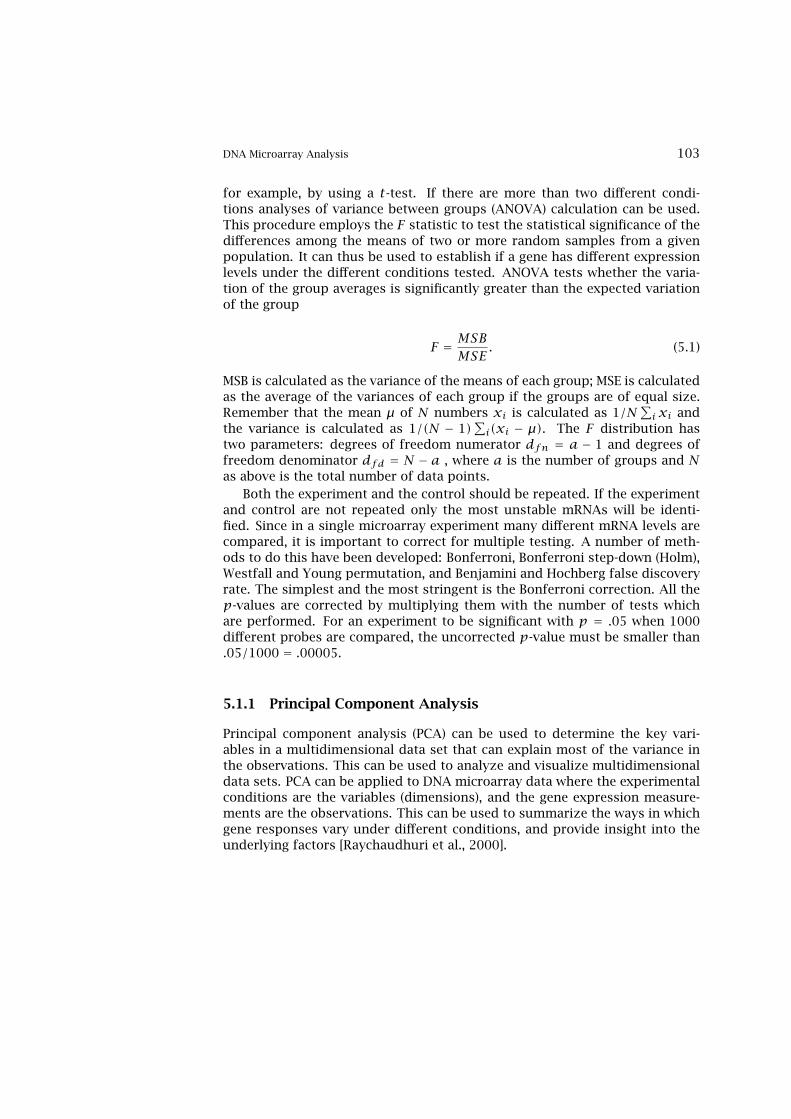
DNA Microarray Analysis 103
for example, by using a t-test. If there are more than two different condi-tions analyses of variance between groups (ANOVA) calculation can be used.This procedure employs the F statistic to test the statistical significance of thedifferences among the means of two or more random samples from a givenpopulation. It can thus be used to establish if a gene has different expressionlevels under the different conditions tested. ANOVA tests whether the varia-tion of the group averages is significantly greater than the expected variationof the group
F = MSBMSE
. (5.1)
MSB is calculated as the variance of the means of each group; MSE is calculatedas the average of the variances of each group if the groups are of equal size.Remember that the mean µ of N numbers xi is calculated as 1/N
∑i xi and
the variance is calculated as 1/(N − 1)∑i(xi − µ). The F distribution has
two parameters: degrees of freedom numerator dfn = a − 1 and degrees offreedom denominator dfd = N − a , where a is the number of groups and Nas above is the total number of data points.
Both the experiment and the control should be repeated. If the experimentand control are not repeated only the most unstable mRNAs will be identi-fied. Since in a single microarray experiment many different mRNA levels arecompared, it is important to correct for multiple testing. A number of meth-ods to do this have been developed: Bonferroni, Bonferroni step-down (Holm),Westfall and Young permutation, and Benjamini and Hochberg false discoveryrate. The simplest and the most stringent is the Bonferroni correction. All thep-values are corrected by multiplying them with the number of tests whichare performed. For an experiment to be significant with p = .05 when 1000different probes are compared, the uncorrected p-value must be smaller than.05/1000 = .00005.
5.1.1 Principal Component Analysis
Principal component analysis (PCA) can be used to determine the key vari-ables in a multidimensional data set that can explain most of the variance inthe observations. This can be used to analyze and visualize multidimensionaldata sets. PCA can be applied to DNA microarray data where the experimentalconditions are the variables (dimensions), and the gene expression measure-ments are the observations. This can be used to summarize the ways in whichgene responses vary under different conditions, and provide insight into theunderlying factors [Raychaudhuri et al., 2000].

104 DNA Microarrays in Immunology
5.2 Clustering
If DNA microarray data are available for several different conditions they canbe used to define clusters of different genes that behave similarly (up- or down-regulated) in different experiments, i.e., under different experimental condi-tions or in different mutant strains. Such genes may be part of a commonpathway and if one of the genes in a group of coregulated genes is known tobe associated with a disease it may indicate that other genes in the group arealso associated with that disease. Even if some related genes are missed (falsenegatives) and unrelated genes are picked up (false positives) the general con-cept of “guilt by association” seems to work [Quackenbush, 2003, Stuart et al.,2003].
Each gene can be represented by N numbers, i.e., an N-dimensional vector,when N experiments are done. The similarity between different genes canbe calculated as a distance in N-dimensional space. The distance betweentwo points x and y in N-dimensional space can be taken to be the Euclidean
distance√∑
i(xi −yi). A better measure is the cosine of the angle between thevectors,
cosα =∑i(xiyi)√∑i x2
i
√∑iy2
i
, (5.2)
since this measure puts less weight on highly expressed genes. Another gooddistance measure is the Pearson correlation coefficient. Different algorithmshave been used to define clusters. UPGMA (unweighted pair group method us-ing arithmetic averages) [Sokal and Michener, 1958, Durbin et al., 1998], neigh-bor joining [Saitou and Nei, 1987, Studier and Keppler, 1988] and K-means[MacQueen, 1967] are often-used clustering methods.
5.2.1 UPGMA Method
The UPGMA method is one of the simplest examples of a hierarchical clus-tering method, i.e., a method where the most similar genes are first groupedtogether. The algorithm is started by letting all data points define their owncluster. Then pairs of clusters with the shortest distance are combined intoone cluster until there is only one cluster.
The distance between two clusters is calculated as the average distancebetween all data points in the first cluster with all data points in the secondcluster. When using UPGMA to draw a tree, all data points are put on a (hori-zontal) line and the nodes combining clusters are put at a height equal to halfthe distance between the clusters.

Clustering 105
5.2.2 Neighbor-Joining
The neighbor-joining algorithm can be seen as an extension of the UPGMAalgorithm. The distance between two points Dij is calculated as dij − (ri + rj)where
ri =1
L− 2
∑kdik. (5.3)
The distance is calculated in this way because the closest neighbors shouldnot always be joined if they have different average distances to other points inthe data set. The description follows that of Durbin et al. [1998].
1. The tree initially consists of all data points as nodes.
2. The pair i, j with the smallest distance Dij is added to the tree as a newnode k with branch lengths dik = 1/2(dij + ri − rj), djk = 1/2(dij − ri +rj) = dij−dik, and distances to other data points dkm = 1/2(dim+djm−dij).
3. k replaces i, j in the list of data points.
4. Repeat steps (2) and (3) until there are two data points left which areconnected with branch length dij .
5.2.3 K-Means
The K-means works by dividing the genes into K clusters and is initialized byrandom assignment of each gene to a cluster. Iteratively the method worksby reassigning all genes to their nearest cluster, until convergence or a givennumber of iterations have been performed. The K-means algorithm differsfrom the ones described above in that it is not hierarchical. A number ofvariants of this algorithm exist. A simple version consists of the following
1. Randomly choosing K genes to define centers.
2. All other genes are assigned to that of the K clusters it is closest to.
3. The K centers are redefined as the average of the genes in the cluster.
4. Steps (2) and (3) are repeated.
106 DNA Microarrays in Immunology
5.3 Immunological Applications
DNA microarrays may be used to monitor which genes are turned on and off inthe host immune system, and in invading pathogens during an infection [Hag-mann, 2000]. This may reveal previously unknown alterations of host geneexpression during infections with viruses [Tong et al., 2004] or with prions[Xiang et al., 2004]. One advantage is that the sample may not even have tocontain the microorganism in question if its effects can be read off from thechanged gene expression of the host [Hagmann, 2000].
Microorganisms may try to escape the host immune response by interferingwith expression of host immune genes. It has, e.g., been shown by microarraystudies that the smallpox virus can modulate the host immune response Ru-bins et al. [2004]. Helminths may also interfere with the immune system: theeggs of the helminth parasite, Schistosoma mansoni, can suppress the abilityof the Toll–like receptor ligand-induced activation of immature dendritic cells[Kane et al., 2004]. Cancer cells may also change the expression of cell surfacemolecules involved in antigen presentation in order to avoid immune surveil-lance [Suscovich et al., 2004].
The difference between the gene expression in vaccinated and nonvacci-nated animals can be elucidated by microarray analysis. Byon et al. [2005]observed significant upregulation of some immune-related genes that are nec-essary for antiviral defense following vaccination with the viral hemorrhagicsepticemia virus glycoprotein. By studying gene expression profiles, they alsofound significant up- and downregulation of unknown genes upon DNA vac-cination. This may be a new basis for establishing the so-called correlates ofprotection, i.e., markers that predict if a vaccine will work or not. Classically,the level of antibodies has often been used as a correlate of protection, butmicroarrays may in the future be used to complement or replace it. More-over, this approach can help us identify other, yet unidentified, players ofprotection. Similar research can be done by comparing naive and immune ani-mal models. For example, Helicobacter pylori-infected mice were characterizedby expression of innate host defense markers while immune mice expressedmany interferon-gamma response genes and T cell markers [Rahn et al., 2004].
A more medical application is to use microarray data to monitor the clini-cal status of patients. This may be important for making decisions on when tostart or change a treatment. A set of genes that are related to the progressionof HIV-1 infection have been identified [Motomura et al., 2004] using microar-ray technology. Such analysis may be used to understand why different indi-viduals have different disease progression speeds. Gene expression profilesof individual patients may be used to design individualized cancer therapies[Kawakami et al., 2004].
Analysis of gene expression profiles may also be used to distinguish differ-

Immunological Applications 107
ent immune cells. Schiott et al. [2004] used gene expression profiles to showthat helper T cell memory populations with or without the CD27 marker areactually functionally different cell populations. Only T cells displaying CD27require costimulation for T cell receptor triggering.


Chapter 6
Prediction of Cytotoxic T Cell(MHC Class I) Epitopes
Cytotoxic T lymphocytes (CTLs) recognize foreign peptides presented on cellsin the body and help to destroy infected or malignant cells. The peptides arepresented by the class I major histocompatibility complex (MHC), and the ac-tual binding of the peptide to the MHC molecules is the single most selectiveevent in the antigen presentation process. The process also includes process-ing (cleavage) of proteins and translocation of peptides from the cytosol intothe endoplasmic reticulum (ER). These latter steps, however, only filter outapproximately four fifths of all potential 9mer peptides, whereas a particularMHC class I allele only binds 1 in 200 potential peptides [Yewdell and Bennink,1999].
The class I MHCs (which are also called class I human leukocyte antigensor HLAs in humans) are encoded by 3 different loci on the genome called A, B,and C. Each of the genes is highly polymorphic and for each locus hundreds ofdifferent alleles exist. The HLAs are thus highly diverse, and each allele binds avery specific set of peptides. All the different alleles can be divided into at least9 supertypes, where the alleles within each supertype exhibit roughly the samepeptide specificity [Sette and Sidney, 1999, Lund et al., 2004]. The concept ofHLA supertypes has great implications for the use of bioinformatical predic-tion algorithms in the search for novel vaccine candidates. The HLA allelespace is very large, and reliable identification of potential epitope candidateswould be an immense task if all alleles were to be included in the search. How-ever, many HLA alleles share a large fraction of their peptide binding reper-toire, and it is often possible to find promiscuous peptides, which bind to aseries of HLA alleles. This allows the search to be limited to a manageable set
109
110 Prediction of MHC Class I epitopes
of alleles. A detailed description of the different HLA supertypes is given inchapter 13.
6.1 Background and Historical Overview of Methods for Pep-tide MHC Binding Prediction
A number of methods for predicting the binding of peptides to MHC moleculeshave been developed (reviewed by Schirle et al. [2001]) since the first motifmethods were presented [Rothbard and Taylor, 1988, Sette et al., 1989b].
The majority of peptides binding to the HLA complex have a length of eightto ten amino acids. For 9mers, positions 2 and 9 are very important for thebinding to most class I HLAs, and these positions are referred to as anchorpositions [Rammensee et al., 1999]. For some alleles the binding motifs furtherhave auxiliary anchor positions. Peptides binding to the A*0101 allele thushave positions 2, 3, and 9 as anchors [Kubo et al., 1994, Kondo et al., 1997,Rammensee et al., 1999].
The importance of the anchor positions for peptide binding and the allele-specific amino acid preference at the anchor positions was first describedby Falk et al. [1991]. The discovery of such allele-specific motifs led to thedevelopment of the first reasonable accurate algorithms [Pamer et al., 1991,Rotzschke et al., 1991]. In these prediction tools, it is assumed that the aminoacids at each position along the peptide sequence contribute a given bind-ing energy, which can independently be added up to yield the overall bindingenergy of the peptide [Parker et al., 1994, Meister et al., 1995, Stryhn et al.,1996]. Similar types of approaches are used by the EpiMatrix method [Schaferet al., 1998], the BIMAS method [Parker et al., 1994], and the SYFPEITHI method[Rammensee et al., 1999]. An example of a peptide binding to an HLA moleculecan be seen in figure 6.1.
These methods cannot take into account correlated effects where the bind-ing affinity of a given amino acid at one position is influenced by amino acidsat other positions in the peptide. Two adjacent amino acids may, e.g., com-pete for the space in a pocket in the MHC molecule. Artificial neural networks(ANN) are ideally suited to take such correlations into account.
Several prediction methods have been made publicly available, includingweight-matrix methods such as BIMAS [Parker et al., 1994] and SYFPEITHI[Rammensee et al., 1999], weight matrices with optimized position-specificweighting [Yu et al., 2002] and ANNs [Brusic et al., 1994, Adams and Koziol,1995]. Recently we have developed a comprehensive HLA-peptide binding pre-diction server including allele-specific weight-matrix predictions for more than120 HLA alleles, as well as ANNs and weight-matrix predictions for 12 allelesrepresenting 12 distinct HLA supertypes. This NetMHC (NetMHC2.0) server is

Background and Historical Overview of Methods for Peptide MHC Binding Prediction 111
A B
Figure 6.1: Example of peptide binding to MHC class I. (A) Cartoon representation of MHC class Ishowing that the peptide is binding to a "floor" made by a β-sheet, and restricted on each side bytwo α-helices. The bound peptide is shown in a sticks representation. B) MHC molecule shownas a molecular surface representation. It can be seen that the binding is closer than it appearsfrom the cartoon model. The figure is based on the PDB (www.rcsb.org/pdb) entry 1q94. Figurecourtesy of Anne Mølgaard. See plate 6 for color version.
available at www.cbs.dtu.dk/services/NetMHC. A more comprehensive list ofservers can be found in chapter 12.
Detailed predictions of peptide binding have been made by dividing bind-ing affinities into classes of affinity ranges; it has been found that the dif-ferent classes are associated with different binding sequence motifs [Adamsand Koziol, 1995]. Neural networks have also been trained to predict MHCbinding using different affinity thresholds [Gulukota et al., 1997]. Mamitsukatrained the transition and emission probabilities of a fully connected hiddenMarkov model (HMM) using a steepest descent algorithm so as to minimizethe differences between the predicted and target probabilities for each pep-tide [Mamitsuka, 1998].
Other prediction algorithms have been developed to predict not only if apeptide binds but also the actual affinity of the binding [Marshall et al., 1995,Stryhn et al., 1996, Rognan et al., 1999, Doytchinova and Flower, 2001, Buuset al., 2003, Nielsen et al., 2003]. For affinity predictions, ANNs in generaloutperform the simpler methods [Gulukota et al., 1997, Nielsen et al., 2003],but generally ANNs need a large number of examples in the training [Yu et al.,2002] to achieve accurate predictions.
Buus et al. [2003] have demonstrated that neural networks trained to per-

112 Prediction of MHC Class I epitopes
form quantitative predictions of peptide MHC binding are superior to con-ventional classification neural networks trained to predict binding vs. non-binding. Nielsen et al. [2003] have further demonstrated that neural networkmethods perform significantly better than linear methods in predicting high-affinity peptides.
A central issue in the development of bioinformatical prediction algorithmsis the number of training examples needed to achieve reliable predictions. Asstated above, ANNs in general need a large number of training data in order toachieve a predictive performance beyond that of the simpler methods. HMMs(or weight matrices), on the other hand, can be trained to a very accurate per-formance on small data sets by use of the techniques described in chapter 4.Common to both artificial networks and HMMs is that both methods rely on theavailability of peptides known to bind a given MHC complex. For many allelessuch data are not available or available only in very limited numbers, and forthese alleles other approaches have to be taken. The number of MHC-peptidecomplexes solved by X-ray crystallography is growing. Based on such struc-tural information, an MHC-peptide binding potential can be derived. Such anapproach has been taken by Altuvia et al. [1995], Schueler-Furman et al. [2000],Doytchinova and Flower [2001] where peptide binding is predicted by eitherfree energy calculations or threading. In situations where no peptide motifinformation exists, these energy-based algorithms are highly valuable.
In this chapter, we will demonstrate how bioinformatical methods can beapplied to derive prediction methods for HLA-peptide binding. In the firstpart, we describe how accurate prediction methods can be derived in situationswhere very limited training data are available. The second part shows howhighly reliable prediction methods can be constructed using a combination ofmany neural networks trained with different sequence encoding schemes.
6.2 MHC Class I Epitope Binding Prediction Trained on SmallData Sets
The highly diverse MHC class I alleles bind very different peptides, and accu-rate binding prediction methods exist only for alleles where the binding pat-tern has been deduced from peptide motifs. Predictions in general tend to bemore precise when more examples are included in the training [Yu et al., 2002],but experimental data on peptides binding to HLA complexes are published inlarge numbers for only a few alleles.
It has earlier been shown that a position specific weighted matrix wherethe weight on selected positions in the matrix describing binding motif is in-creased performs slightly better for A*0201 predictions than an unweightedmatrix [Yu et al., 2002]. A similar result was found in the example for weight-
MHC Class I Epitope Binding Prediction Trained on Small Data Sets 113
matrix construction in chapter 4, where a weight matrix was constructed from10 HLA-A*0201 restricted peptide using the technique of sequence weighting,pseudocount correction for low counts, and position-specific weighting. Thismatrix was shown to share many of the features of a weight matrix trainedon close to 500 HLA-A*0201 restricted peptides. It is, however, not clear fromthese two examples to what extent such a weighting will influence the numberof data needed to generate accurate predictors.
In the following section, we will describe a method for predicting whichpeptides bind to given MHC class I alleles based on scoring matrices with em-pirical position specific anchor weighting.
6.2.1 Weight-Matrix Training
The selected peptides can be stacked into a multiple alignment and using anungapped HMM-like approach the log-odds weight matrix was calculated aslog(ppa/qa), where ppa is the frequency of amino acid a at position p inthe alignment and qa the background frequency of that amino acid in theSwiss-Prot database [Henikoff and Henikoff, 1994]. The values for ppa wereestimated using the techniques of sequence weighting and pseudocount cor-rection for low counts described in chapter 4 [Altschul et al., 1997, Henikoffand Henikoff, 1992]. A schematic view of the procedure is outlined in figure6.2. To analyze how the predictive performance of a weight matrix dependson the number of training data, we varied the numbers of peptides includedto calculate the weight matrix. For each number of training peptides, 200 datasets were constructed, using the bootstrap procedure [Press et al., 1992], byrandomly drawing the chosen number of peptides with replacement from theoriginal data set of peptides.
To visualize the problem one is facing when training a prediction methodon limited amounts of data, we generated sequence logos for peptides bindingto the A*0201 allele using 10 and 100 peptides, respectively. From the logoconstructed using 10 random A*0201 binding peptides (figure 6.3A), it can beseen that the importance of the anchor positions 2 and 9 is not yet visible,while this feature is clearly apparent in the logo based on 100 sequences (fig-ure 6.3B). The amino acid preferences for the hydrophobic amino acids L andL/V at positions 2 and 9, respectively, is, however, present in both logos. Basedon the information content visualized with the logos in figure 6.3, a predictionmethod trained on very little data would very likely benefit by incorporatingthe prior knowledge about the differential importance of the different posi-tions in the motif. This is naturally done by increasing the relative weight onthe anchor positions. The logo of a matrix with position-specific differentialweighting at positions 2 and 9 is shown in figure 6.3C.
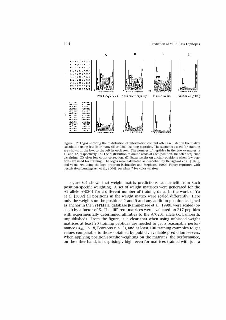
114 Prediction of MHC Class I epitopes
Figure 6.2: Logos showing the distribution of information content after each step in the matrixcalculation using few (I) or many (II) A*0301 training peptides. The sequences used for trainingare shown in the box to the left in each row. The number of peptides in the two examples is10 and 32, respectively. (A) The distribution of amino acids at each position. (B) After sequenceweighting. (C) After low count correction. (D) Extra weight on anchor positions when few pep-tides are used for training. The logos were calculated as described by Hebsgaard et al. [1996],and visualized using the logo program [Schneider and Stephens, 1990]. Figure reprinted withpermission [Lundegaard et al., 2004]. See plate 7 for color version.
Figure 6.4 shows that weight matrix predictions can benefit from suchposition-specific weighting. A set of weight matrices were generated for theA2 allele A*0201 for a different number of training data. In the work of Yuet al. [2002] all positions in the weight matrix were scaled differently. Hereonly the weights on the positions 2 and 9 and any addition position assignedas anchor in the SYFPEITHI database [Rammensee et al., 1999], were scaled (bi-ased) by a factor of 5. The different matrices were evaluated on 217 peptideswith experimentally determined affinities to the A*0201 allele (K. Lamberth,unpublished). From the figure, it is clear that when using unbiased weightmatrices at least 20 training peptides are needed to get a reasonable perfor-mance (AROC > .8, Pearsons r > .5), and at least 100 training examples to getvalues comparable to those obtained by publicly available prediction servers.When applying position-specific weighting on the matrices, the performance,on the other hand, is surprisingly high, even for matrices trained with just a
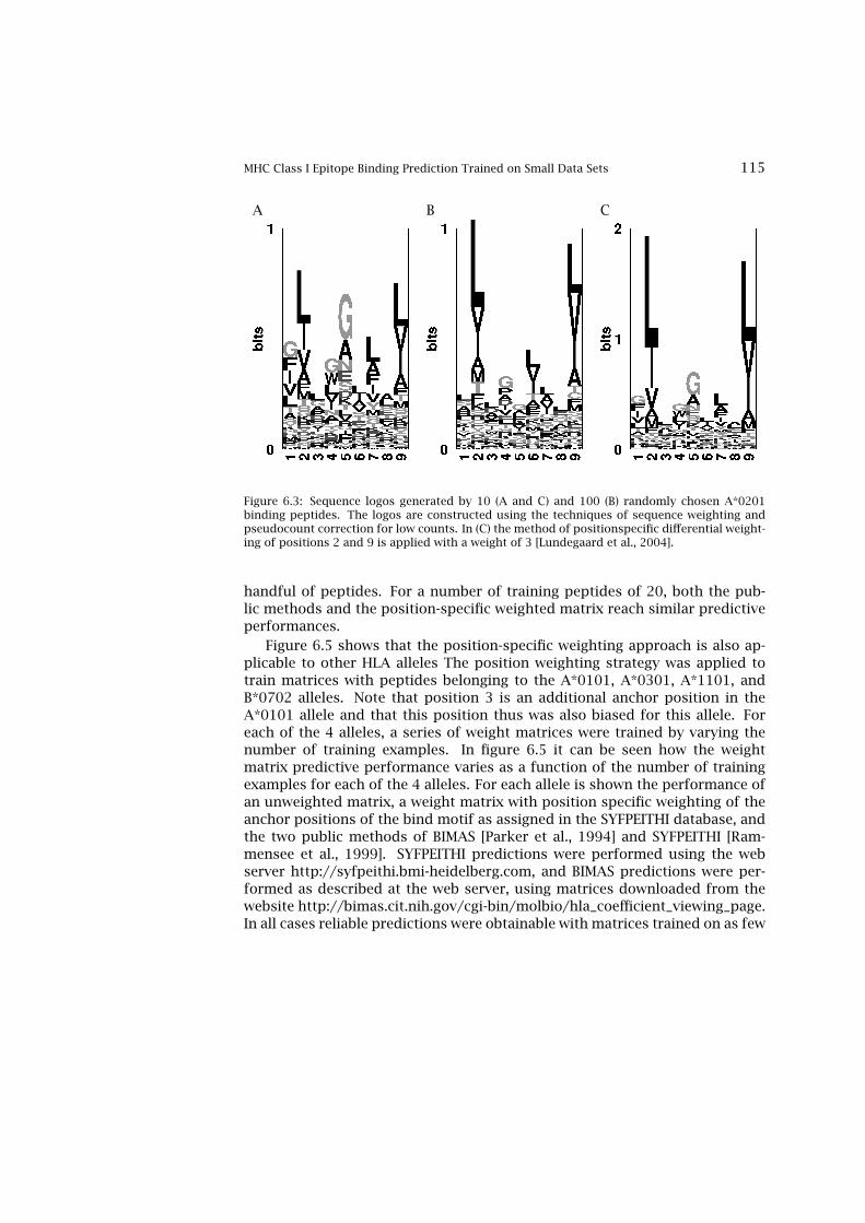
MHC Class I Epitope Binding Prediction Trained on Small Data Sets 115
A B C
Figure 6.3: Sequence logos generated by 10 (A and C) and 100 (B) randomly chosen A*0201binding peptides. The logos are constructed using the techniques of sequence weighting andpseudocount correction for low counts. In (C) the method of positionspecific differential weight-ing of positions 2 and 9 is applied with a weight of 3 [Lundegaard et al., 2004].
handful of peptides. For a number of training peptides of 20, both the pub-lic methods and the position-specific weighted matrix reach similar predictiveperformances.
Figure 6.5 shows that the position-specific weighting approach is also ap-plicable to other HLA alleles The position weighting strategy was applied totrain matrices with peptides belonging to the A*0101, A*0301, A*1101, andB*0702 alleles. Note that position 3 is an additional anchor position in theA*0101 allele and that this position thus was also biased for this allele. Foreach of the 4 alleles, a series of weight matrices were trained by varying thenumber of training examples. In figure 6.5 it can be seen how the weightmatrix predictive performance varies as a function of the number of trainingexamples for each of the 4 alleles. For each allele is shown the performance ofan unweighted matrix, a weight matrix with position specific weighting of theanchor positions of the bind motif as assigned in the SYFPEITHI database, andthe two public methods of BIMAS [Parker et al., 1994] and SYFPEITHI [Ram-mensee et al., 1999]. SYFPEITHI predictions were performed using the webserver http://syfpeithi.bmi-heidelberg.com, and BIMAS predictions were per-formed as described at the web server, using matrices downloaded from thewebsite http://bimas.cit.nih.gov/cgi-bin/molbio/hla_coefficient_viewing_page.In all cases reliable predictions were obtainable with matrices trained on as few

116 Prediction of MHC Class I epitopes
Figure 6.4: Curves of the AROC value (major graph) and the Pearson correlation coefficient(inserted graph) plotted against the number of training examples randomly selected from thetotal pool of peptides. Each value is the simple average of 200 independent calculations with theindication of one standard deviation. The matrices were generated and evaluated with peptidesbinding to the allele A*0201. The score for a given peptide is calculated as the sum of the scoresat each position. Training examples were extracted from the databases SYFPEITHI [Rammenseeet al., 1999] and MHCPEP [Brusic et al., 1998a]. As evaluation sets, we used peptides for which theaffinities for the selected alleles had been measured using the enzyme-linked immunosorbentassay (ELISA) method described by Sylvester-Hvid et al. [2002] (K. Lamberth, unpublished) usinga threshold for binders of 500 nM. Predictions were made for the corresponding evaluation setby each of the 200 matrices of each train set size, and the predictive performance was measuredin terms of both the linear (Pearson) correlation coefficient between the prediction output andlog-transformed measured affinities [Buus et al., 2003] and the area under a receiver operatingcharacteristic (ROC) curve, the AROC value [Swets, 1988]. The final predictive performance isgiven as the simple average of the 200 values. Figure reprinted with permission [Lundegaardet al., 2004].

MHC Class I Epitope Binding Prediction Trained on Small Data Sets 117
Figure 6.5: Curves of the AROC value (major graph) and the Pearson correlation coefficient (in-serted graph) plotted against the number of training examples randomly selected from the totalpool of peptides. Each value is the simple average of 200 independent calculations with theindication of one standard deviation. The matrices were generated and evaluated with peptidesbinding to the alleles A*0101, A*0301, A*1101, and B*0702. Note that the SYFPEITHI A*1101predictions were generated using the A03 predictor. Figure reprinted with permission [Lunde-gaard et al., 2004].
as 5 training examples. For all alleles the performance of the position-specificweighted matrix is comparable to that of the public methods when 20 trainingexamples are available.
Table 6.1 shows the prediction accuracy for predictors for different alleleson severe acute respiratory syndrome (SARS) derived peptides [Sylvester-Hvidet al., 2004] and on peptides from evaluation sets obtained from the MHCBN3.1 database [Bhasin et al., 2003]. In the evaluation the predictive performancein terms of the AROC value was calculated for each of the evaluation sets us-ing position-specific weight matrices trained on different numbers of data; anunweighted matrix trained on all available data; and the two public methods,BIMAS and SYFPEITHI.

118 Prediction of MHC Class I epitopes
Allele Matrix Biased matrix Biased matrix Biased matrix BIMAS SYFPEITHIall peptides 5 peptides 20 peptides all peptides
A*01011 1.000 0.992 ± 0.026 1.000 ± 0.002 1.000 1.000 1.000A*02011 0.925 0.803 ± 0.024 0.830 ± 0.017 0.871 0.907 0.864A*01012 0.963 0.986 ± 0.011 0.992 ± 0.004 0.997 0.951 0.987A*02012 0.992 0.973 ± 0.015 0.978 ± 0.006 0.984 0.979 0.970A*03012 0.912 0.885 ± 0.072 0.873 ± 0.028 0.877 0.857 0.829A*11012 0.937 0.914 ± 0.038 0.948 ± 0.018 0.968 0.950 0.8303
B*07022 0.983 0.972 ± 0.013 0.977 ± 0.009 0.985 0.990 0.990B*15012,4 0.928 0.932 ± 0.039 N.A. 0.955 0.893 N.A.B*58012,4 0.892 0.959 ± 0.008 N.A. 0.959 0.994 N.A.
Table 6.1: Evaluation of 200 matrices made by selecting 5 or 20 peptides respectively, by thebootstrap method, or a single matrix generated by all available different peptides from MHCPEPand SYFPEITHI databases. The performance was measured in terms of the AROC value. Evalua-tion was performed with peptides extracted from the MHCBN 3.11 database, and SARS2 relevantpeptides. 3 Predictions were made using the A03 predictor. 4 The bootstrapping procedure wasnot used due to the small total number of peptides available. Instead, all possible combinationsof the available peptides were used to estimate the standard deviation. Table adapted fromLundegaard et al. [2004].
The analysis confirms that a weight matrix with position specific weightingof the anchor position trained on 20 peptide examples achieves a predictiveperformance comparable to that of BIMAS and SYFPEITHI. In many cases theperformance for a biased matrix trained on only 5 peptide examples is compa-rable to that of the two public methods.
In summary, we have shown that the empirical knowledge of importantanchor positions within the binding motif dramatically reduces the number ofpeptides needed for reliable predictions. The method leads to predictions witha comparable or higher accuracy than other established prediction servers,even in situations where only very limited data are available for training.
6.3 Prediction of CTL Epitopes by Neural Network Methods
Having described how accurate weight matrix–based methods can be derivedwhen very limited training data are available, we now focus on situations wherethe training set is large. In such situations neural networks would be the choiceof method.
Neural network methods for predicting whether or not a peptide binds MHCmolecules have earlier been developed [Brusic et al., 1994, Buus et al., 2003]. Inthis section we will describe how prediction of MHC I binding peptides may beimproved using methods that combine several neural networks, each derivedusing different sequence encoding schemes.
Brusic et al. use a conventional sparse (orthogonal) encoding of the 20-
Prediction of CTL Epitopes by Neural Network Methods 119
amino acid alphabet as well as 6- and 9-letter reduced alphabets [Brusic et al.,1994]. The conventional sparse encoding of the amino acids ignores theirchemical similarities. We shall use a combination of several sequence-encodingstrategies in order to take these similarities into account explicitly. The differ-ent encoding schemes are defined in terms of BLOSUM matrices and hiddenMarkov models in addition to the conventional sparse encoding. The input tothe neural network can consist of a combination of sparse encoding, BLOSUMencoding, and input derived from HMMs. We will show that this can lead toa performance superior to neural networks derived using a single sequence-encoding scheme, especially for the high-affinity binding peptides.
We start by demonstrating that peptides binding to the HLA-A*0204molecule display signals of higher-order sequence correlations; next we traina series of ANNs using different sequence-encoding schemes, and demonstratehow the combination of many such diverse networks improves the predictionaccuracy. In the last part of the section we apply the neural network algorithmto perform a genome-wide search for potential CTL epitopes in the genome ofthe hepatitis C virus (HCV).
6.3.1 Experimental Data
Two sets of data were used to derive the prediction method. One set was usedto train and test the neural networks, and consists of 528 9-mer amino acidpeptides for which the binding affinity to the HLA class I molecule A*0204 hasbeen measured by the method described by Buus et al. [1995]. This data setis hereinafter referred to as the Buus data set. The second data set was usedto train the HMM. This data set was constructed from sequences downloadedfrom the SYFPEITHI database [Rammensee et al., 1995]. All sequences fromthe database were downloaded and clustered into the nine supertypes (A1,A2, A3, A24, B7, B27, B44, B58, and B62) and 3 outlier types (A29, B8, andB46) described by Sette and Sidney [1999]. The sequences in the A2 supertypecluster were aligned manually and trimmed into 211 unique 9-amino acid longpeptides. This data set is hereinafter referred to as the Rammensee data set.
6.3.2 Mutual Information
One important difference between linear prediction methods like first-orderHMMs and nonlinear prediction methods like neural networks with hiddenlayers is their capability to integrate higher-order sequence correlations intothe prediction score. A measure of the degree of higher-order sequence corre-lations in a set of aligned amino acid sequences can be obtained by calculatingthe mutual information matrix. For the case of peptide 9-mers, this is a 9 x

120 Prediction of MHC Class I epitopes
9 matrix where each matrix element is, as described in Chapter 4, calculatedusing the formula
Mij =∑a
∑bPij(ab) log
Pij(ab)Pi(a)Pj(b)
. (6.1)
In this example the summation is over the 20 letters in the conventional aminoacid alphabet and i, j refer to positions in the peptide. Pij(ab) is the prob-ability of mutually finding the amino acid a at position i and amino acid bat position j. Pi(a) is the probability of finding amino acid a at position iirrespective of the content at the other positions, and likewise for Pj(b). Apositive value in the mutual information matrix indicates that prior knowl-edge of the amino acid content at position i will provide information aboutthe amino acid content at position j. The statistical reliability of a mutualinformation calculation relies crucially on the size of the corresponding dataset. In the mutual information calculation one seeks to estimate 400 aminoacid pair frequencies at each position in the matrix. Such estimates are nat-urally associated with large uncertainties when dealing with small data sets.Figure 6.6 shows the mutual information matrix calculated for two differentsets of 9-mer alignments.
The first data set was constructed to obtain the largest possible positive set,by combining peptides from the Rammensee data set with the peptides fromthe Buus data set that were measured to bind MHC (i.e., having a KD < 500nM). This set contains 313 unique sequences. The second data set was con-structed as a negative set by extracting 313 unique random peptides from theMycobaterium tuberculosis genome. The mutual information content is calcu-lated using the conventional 20-amino acid alphabet. The figure demonstratesa signal of mutual information between the seven nonanchor residues posi-tions (1, 3, 4, 5, 6, 7, and 8) in the data set defined by peptides that bind tothe HLA molecule. It is worth remarking that the mutual information contentbetween any of the two anchor positions (2 and 9) and all other amino acidsis substantially lower than the mutual information content between any twononanchor positions.
6.3.3 Combination of More than One Neural Network Prediction
We combine the output from the two networks trained using sparse and BLO-SUM sequence encoding, respectively, in a simple manner, as a weighted sumof the two. To select the weight that corresponds to the optimal performance,we plot the sensitivity/PPV as well as the ROC (relative operating characteris-tic) curves [Swets, 1988] for a series of weighted sum combinations of the twonetwork outputs. The sensitivity is defined as the ratio TP/AP. Here TP (true

Prediction of CTL Epitopes by Neural Network Methods 121
Figure 6.6: Mutual information matrices calculated for two different data sets. The leftpanel shows the mutual information matrix calculated for a data set consisting of 313 pep-tides derived from the Rammensee data set combined with binding peptides from the Buusdata set (defined as KD < 500 nM). The right panel shows the mutual information matrixcalculated for a set of 313 random peptides extracted from the Mycobaterium tuberculosisgenome [Nielsen et al., 2003]. The plot was made using MatrixPlot [Gorodkin et al., 1999](http://www.cbs.dtu.dk/services/MatrixPlot/).
positives) is the number of data points for which both the predicted score isabove a given prediction threshold value and the measured binding affinity isabove a given classification threshold value. AP (actual positives) is the totalnumber of data points that have a measured binding affinity above the affin-ity threshold value. The PPV is defined as the ratio TP/PP. Here PP (predictedpositives) is the total number of predictions with scores above the predic-tion threshold value. The PPV is a measure of the reliability of the predictionmethod. The ROC curves are closely related to the sensitivity/PPV curves, butwith the important difference that one of the axis in the ROC curve is thefalse-positive proportion FP/AN (actual negatives) and not the true positive-to-predicted positive ratio (the PPV). The area under the ROC curve (AROC )provides an estimate of the accuracy of the prediction method. A randommethod will have a value of AROC = 0.5. AROC > 0.8 indicates that the methodhas moderate accuracy and AROC = 1, that the prediction method is perfect[Swets, 1988]. In a sensitivity/PPV plot, the curve for the perfect method is theone where the area under the curve is unity. The curves are estimated using

122 Prediction of MHC Class I epitopes
Figure 6.7: (a) Sensitivity/PPV plot calculated using a classification binding affinity of 500 nM fora series of linear combinations of the two neural network methods corresponding to BLOSUM50and sparse sequence encoding, respectively. The curves were calculated by use of the bootstrapmethod [Press et al., 1992] using 500 data set realizations. (a) 428 peptides in the test/train dataset; (b) 100 peptides in the evaluation set. In the upper graph we determine the optimal per-formance to be the thick blue curve, corresponding to a combination of the two neural networkmethods with 70% weight on the BLOSUM50 encoded prediction and 30% weight on the sparseencoded prediction. This set of weights also results in close to optimal performance in the lowergraph. Inserts to the graphs show the corresponding ROC curves. Figure adapted from Nielsenet al. [2003].
the bootstrap method [Press et al., 1992]. N data sets were constructed byrandomly drawing M data points with replacement from the original data setof M peptides. For each of the N data sets a sensitivity/PPV curve and a ROCcurve was calculated and the curves displayed in figure 6.7 are derived fromthe mean of these N sensitivity/PPV and ROC curve realizations.
In figure 6.7, the sensitivity/PPV curves for the 428 peptides in the train andtest set and the 100 peptides in the evaluation set are shown for a measuredbinding affinity threshold value equal to 0.426, corresponding to a bindingaffinity of 500 nM. In the inserts to the figures the corresponding ROC curvesare shown. From the figure, it is clear that both the sparse and the BLOSUMencoded neural networks have a performance that is inferior to any combi-nation of the two. In figure 6.7(a) the optimal combination is found to havea weight on the BLOSUM encoded network close to 0.7 and a weight on thesparse encoded network close to 0.3. This set of weights for the combinationof the two neural network predictions is also, in figure 6.6(b), seen to improveto the prediction accuracy for the 100 peptides in the evaluation set. Thisis, however, less obvious, due to the small number of binding peptides in theevaluation set. The evaluation set contains 31 peptides with binding affinitystronger than 500 nM.
Prediction of CTL Epitopes by Neural Network Methods 123
The Pearson correlation coefficient between the predicted and the mea-sured binding affinities for the sparse encoded, the BLOSUM encoded, and thecombined neural network method on the peptides in the train/test set is foundto be .849, .887 and .895, respectively. For the peptides in the evaluation setthe corresponding values are found to be .866, .926, and .928 respectively.
The neural network training and testing is next repeated using the full dataset in a fivefold cross-validation. The combined method, hereinafter referredto as comb-I, is defined using the weights on the BLOSUM and the sparse en-coded neural networks, respectively, estimated above.
6.3.4 Integration of Data from the Rammensee Database in the Neu-ral Network Training
In figure 6.8(b), we show the performance of the HMM evaluated on the 528peptides in the Buus data set. The figure displays a reasonable correlationbetween the HMM score and the measured binding affinity. This correlationdemonstrates that the sequences in the Rammensee data set contain valuableinformation and that the neural network training could benefit from an inte-gration of the Rammensee sequence data into the training data set. It is, how-ever, not obvious how such an integration should be done. The Rammenseedata are binary in nature. They describe that a given peptide does bind to theHLA molecule but not the strength of the binding. The data in the Buus dataset, on the other hand, are continuous in that each peptide is associated witha binding affinity. It turns out that a fruitful procedure for integrating theRammensee data into the neural network training is to use the output scoresgenerated by the HMM as additional input to the neural network. The HMM istrained on the peptides in the Rammensee data set. The model is nine residueslong, and the scores used as input to the neural network are the nine scoresobtained when aligning a 9-mer peptide to the model. Two neural networkseach with 189 input neurons (180 for sequence encoding and 9 to encode thescores from the HMM) are trained in a fivefold manner as described above us-ing the HMM scores combined with the sparse or BLOSUM sequence encodingin the input layer, respectively. In the final combined method, the predictionvalue is calculated as the simple average with equal weight of the sparse andBLOSUM encoded neural network predictions, respectively.
This method is hereinafter referred to as comb-II and is the one used in theHCV genome predictions described below.

124 Prediction of MHC Class I epitopes
Figure 6.8: Scatterplot of the predicted score vs. the measured binding affinity for the 528peptides in the Buus data set. The figure shows the performance for four different predictionmethods. The insert to each figure shows an enlargement of the part of the plot that corre-sponds to a binding affinity stronger than 500 nM. (a) Rammensee matrix method, (b) HMMtrained on sequences in the Rammensee data set, (c) Neural network trained with sparse se-quence encoding, and (d) The comb-II neural network method. The straight-line fit to the datain (c) and (d) have slope and intercept of 0.989, -0.029, and 0.979, -0.027, respectively. Figurereprinted with permission [Nielsen et al., 2003].
6.3.5 Neural Network Methods Compared to HMM Methods and theMatrix Method of Rammensee
In table 6.2, we give the test performance measured in terms of the Pearsoncorrelation coefficient for the 528 peptides in the Buus data set for six dif-ferent prediction methods: One method is the matrix method of Rammenseeet al. [1999]; the second, the HMM trained on the Rammensee data set; andthe other four, neural networks methods trained using sparse and BLOSUMsequence encoding, the linear combination of the two, and the linear combi-nation including input from the HMM, respectively. For the matrix methodof Rammensee and the HMM, we calculate the Pearson correlation between

Prediction of CTL Epitopes by Neural Network Methods 125
Method Pearson (all) Pearson (500 nM) Pearson (50 nM)Rammensee 0.761 ± 0.016 0.296 ± 0.073 0.066 ± 0.116HMM 0.804 ± 0.014 0.332 ± 0.061 0.142 ± 0.096NNSparse 0.877 ± 0.011 0.438 ± 0.065 0.345 ± 0.090NNBl50 0.899 ± 0.010 0.498 ± 0.064 0.382 ± 0.099Comb-I 0.906 ± 0.009 0.508 ± 0.063 0.392 ± 0.092Comb-II 0.912 ± 0.009 0.508 ± 0.054 0.420 ± 0.080
Table 6.2: The Pearson correlation coefficient between the predicted score and the measuredbinding affinity for the 528 peptides in the Buus data set. The six methods in the table areRammensee: Score matrix method by H. G. Rammensee; HMM: hidden Markov model trainedon sequence data in the Rammensee data set; NNSparse: neural network with sparse sequenceencoding; NNBL50: neural network with BLOSUM50 sequence encoding; Comb-I: combination ofneural network trained using sparse and BLOSUM50 sequence encoding, respectively; and Comb-II: combination of neural network trained using sparse, BLOSUM50, and HMM sequence encod-ing, respectively. The numbers given in the table are calculated using the bootstrap method[Press et al., 1992] with 500 data set realizations. The correlation values are estimated as av-erage values over the 500 data set realizations and the associated standard deviations. Tableadapted from Nielsen et al. [2003].
the raw output scores and the logarithmically transformed measured bindingaffinities even though this might not be what optimally relates the predictionscore to the measured binding affinity.
From the results shown, it is clear that the neural network methods all havea higher predictive performance compared to both the method of Rammenseeand the HMM. The difference in predictive performance between the neuralnetwork and the Rammensee and the HMM methods is most significant fordata sets defined by peptides with a binding affinity stronger than 50 nM,thus indicating that the signal of higher-order sequence correlation is moststrongly present in peptides that bind strongly to the HLA A2 molecule. Thesame conclusion can be drawn from the data displayed in figure 6.8. Herethe test performance for the 528 peptides is shown as a scatterplot of theprediction score vs. the measured binding affinity for four of the six methodsabove. Again, it is clear that the neural network methods in general and thecombined methods in particular have a higher predictive performance thanthe Rammensee and the HMM methods. The least-squares straight-line fit tothe data shown in figure 6.8 (c) and (d) also validates the quality and accuracyof the neural network predictions. In the two plots the straight line fits havea slope and intercept of 0.989,−0.029 and 0.979,−0.027, respectively, thusdemonstrating the strength of the neural network trained on quantitative datain providing a direct relationship between the neural network output and themeasured binding affinity.
In figure 6.9, we show the sensitivity/PPV curves calculated for the data in
126 Prediction of MHC Class I epitopes
the 528 peptide set using the four different neural network methods as wellas the method of Rammensee and the HMM method. All curves are estimatedusing the bootstrap method described above. The upper graph shows the sen-sitivity/PPV curves for the six methods calculated for a classification thresh-old corresponding to 500 nM, and the lower graph shows the sensitivity/PPVcurves for a classification threshold corresponding to 50 nM. In the inserts tothe graphs are shown the corresponding ROC curves for the six methods. Inthe labels to the curves in the inserts, we give the estimated ROC areas [Swets,1988]. In both graphs, it is clear that the combined neural methods have a per-formance superior to that of the other four methods. All four neural networkmethods and in particular the two combined methods have a performance thatis substantially higher than that of the Rammensee method. The ranking ofthe six methods obtained using the ROC area method is identical to the rank-ing estimated using the Pearson correlation measure given in table 6.2. Usinga Student’s t-test to compare the mean error of prediction (predicted bindingaffinity − measured binding affinity) between the comb-II method and the twoneural network methods trained with a single sequence encoding, we find thatthe p-values are less than 10−4 and .005 for sparse and BLOSUM sequenceencoding, respectively. The individual schemes for ranking the different meth-ods thus all confirm that the combination of several neural network methodstrained with different sequence representations has a performance superiorto any neural network trained with a single sequence representation. Figure6.9 further demonstrates that the integration of the data from the Rammenseedatabase in the training of the neural networks, in terms of the HMM inputdata, increases the reliability of the combined neural network method sub-stantially. For an affinity threshold of 500 nM the plot shows that at a PPV of0.975 the combined neural network method comb-II has a sensitivity of 0.54,where the combined neural network method comb-I, which does not includeHMM data, has a sensitivity of only 0.22. In figure 6.9(a) the largest sensitivitygap between the combined neural method (Comb-II) and the method of Ram-mensee is found at a PPV equal to 0.7, corresponding to a difference of 0.38 insensitivity or a difference in the number of true-positive predictions of 29 of atotal of the 76 high binding peptides in the data set. In figure 6.9(b) the largestsensitivity gap between the two methods is found at a PPV equal to 0.88, corre-sponding to a difference of 0.37 in sensitivity or a difference in the number oftrue-positive predictions of 54 of a total of 144 intermediate binding peptidesin the data set.
Both the method of Rammensee and the HMM are linear methods derivedfrom binary affinity data. Neural networks can, on the other hand, both trainon data with continuous binding affinities and, if a hidden layer is contained,include higher-order sequence correlations in the output score. To estimatethe importance of the ability of the neural network to train on continuous data

Prediction of CTL Epitopes by Neural Network Methods 127
Figure 6.9: Sensitivity/PPV curves calculated from the 528-peptide data set. Six methods areshown in the graphs: Rammensee: matrix method by Rammensee et al. [1999]; HMM: hiddenMarkov Model trained on data from the Rammensee database; SEQ: neural network with sparsesequence encoding; Bl50: neural network with BLOSUM50 sequence encoding; Comb-I: combina-tion of neural network trained with sparse and BLOSUM50 sequence encoding, respectively; andComb-II: combination of neural network with sparse, BLOSUM50, and HMM sequence encoding.The upper graph (a) shows the curves for a classification affinity threshold of 50 nM. The lowergraph (b) shows the curves corresponding to a classification affinity threshold of 500 nM. Thesensitivity/PPV curves were calculated as described in figure 6.8 using 528 data set realizations.In the inserts to the graphs are shown the ROC curves defined in the text. The values given withthe labels to each of the curves in the inserts are the area under the ROC curves. Figure adaptedfrom Nielsen et al. [2003].
and the importance of integration of higher-order sequence correlations in theprediction score, we transformed the Buus data set into binary data by assign-ing peptides with a measured binding affinity stronger than 500 nM an outputvalue of 0.9, and all other peptides a value of 0.1. In a fivefold cross-validationof a neural network using sparse sequence encoding the test performance onthe 528 peptides in the Buus data set was found to be 0.838 ± 0.013 and 0.856± 0.013 for networks trained without and with a hidden layer, respectively.These numbers should be compared to the 0.877 ± 0.011 obtained for a neu-ral network with a hidden layer trained and tested in a similar manner usingcontinuous affinity data. The result hence confirms the importance of bothtraining the prediction method on data with continuous binding affinities andthe ability of the neural network method to integrate higher-order sequencecorrelation in the prediction score.
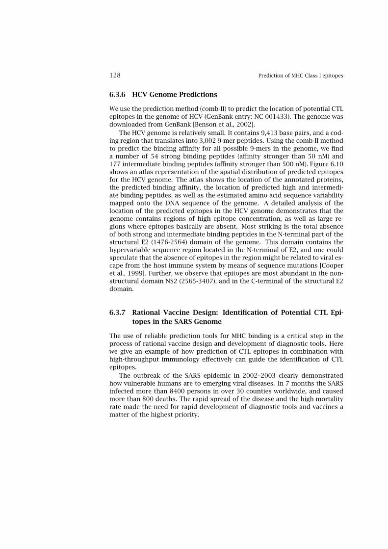
128 Prediction of MHC Class I epitopes
6.3.6 HCV Genome Predictions
We use the prediction method (comb-II) to predict the location of potential CTLepitopes in the genome of HCV (GenBank entry: NC 001433). The genome wasdownloaded from GenBank [Benson et al., 2002].
The HCV genome is relatively small. It contains 9,413 base pairs, and a cod-ing region that translates into 3,002 9-mer peptides. Using the comb-II methodto predict the binding affinity for all possible 9-mers in the genome, we finda number of 54 strong binding peptides (affinity stronger than 50 nM) and177 intermediate binding peptides (affinity stronger than 500 nM). Figure 6.10shows an atlas representation of the spatial distribution of predicted epitopesfor the HCV genome. The atlas shows the location of the annotated proteins,the predicted binding affinity, the location of predicted high and intermedi-ate binding peptides, as well as the estimated amino acid sequence variabilitymapped onto the DNA sequence of the genome. A detailed analysis of thelocation of the predicted epitopes in the HCV genome demonstrates that thegenome contains regions of high epitope concentration, as well as large re-gions where epitopes basically are absent. Most striking is the total absenceof both strong and intermediate binding peptides in the N-terminal part of thestructural E2 (1476-2564) domain of the genome. This domain contains thehypervariable sequence region located in the N-terminal of E2, and one couldspeculate that the absence of epitopes in the region might be related to viral es-cape from the host immune system by means of sequence mutations [Cooperet al., 1999]. Further, we observe that epitopes are most abundant in the non-structural domain NS2 (2565-3407), and in the C-terminal of the structural E2domain.
6.3.7 Rational Vaccine Design: Identification of Potential CTL Epi-topes in the SARS Genome
The use of reliable prediction tools for MHC binding is a critical step in theprocess of rational vaccine design and development of diagnostic tools. Herewe give an example of how prediction of CTL epitopes in combination withhigh-throughput immunology effectively can guide the identification of CTLepitopes.
The outbreak of the SARS epidemic in 2002–2003 clearly demonstratedhow vulnerable humans are to emerging viral diseases. In 7 months the SARSinfected more than 8400 persons in over 30 counties worldwide, and causedmore than 800 deaths. The rapid spread of the disease and the high mortalityrate made the need for rapid development of diagnostic tools and vaccines amatter of the highest priority.
Prediction of CTL Epitopes by Neural Network Methods 129
Figure 6.10: Epitope atlas for the hepatitis C virus. The inner thin (blue) circle shows the locationof annotated proteins. the broader circles represent from the center and out: the location of highbinding peptides, the location of intermediate binding peptides, the predicted binding affinityvalue, and the the sequence variability, respectively. The atlas is plotted using the ”Genewiz”program of H.H. Staerfeldt. See plate 8 for color version.
At the height of the SARS epidemic in the spring of 2003, we performeda complete genome-wide scan covering all (at that time known) 9 HLA super-types (covering > 99% of all major human populations). The SARS genomecontains close to 10,000 unique 9mer peptides. To identify potential CTL epi-topes we applied the method of ANNs and weight matrices. For each HLAsupertype, we selected the top 15 candidates for tests in biochemical bindingassays. From the 10,000 peptides we thus selected 135 for biochemical valida-tion. The biochemical validation consists of a binding experiment, where thebinding affinity between the MHC molecule and the selected peptide is mea-sured in an ELISA experiment [Sylvester-Hvid et al., 2002]. Following this ap-proach, we identified more than 100 potential vaccine candidates, and rapidlyidentified more than 100 potential SARS CTL epitopes [Sylvester-Hvid et al.,2004]. In figure 6.11, we show a graphical representation of the predicted CTL

130 Prediction of MHC Class I epitopes
Figure 6.11: Circular epitope map of the linear genome of the SARS coronavirus. From the centeroutward: indexed RNA, translated regions, observed sequence variation, predicted proteasomalcleavage, predicted A1 epitopes, predicted A*0204 epitopes, predicted A*1101 epitopes, pre-dicted A24 epitopes, predicted B7 epitopes, predicted B27 epitopes, predicted B44 epitopes,predicted B58 epitopes, and predicted B62 epitopes. Figure is a permitted reprint of the coverfigure of Tissue Antigens vol. 64 issues 2-4, related to the paper by Sylvester-Hvid et al. [2004].See plate 9 for color version.
epitopes in the SARS genome for the 9 supertypes. Also included in the figureis the sequence variability in the SARS genome and the predicted proteasomalcleavage. At the conclusion of this study, the SARS epidemic had ended andwe were unable to get access to patients and test our putative epitopes.

Summary of the Prediction Approach 131
6.4 Summary of the Prediction Approach
When trained on very limited positive examples, matrices and other predictionmethods do not contain sufficient information to distinguish between impor-tant and less important positions in the binding motif. Empirical knowledge ofpositions in the motifs that are known to be the most informative can there-fore often guide the predictions if the relative weight of these positions isincreased. Applying this approach it is possible to obtain reliable predictionsof MHC class I binding peptides, even when the allele in question is poorlyinvestigated and few binding examples exist.
When more data are available, ANN methods can be trained to predict MHC-peptide binding with a high reliability. Neural networks can take higher-ordersequence correlations into account when predicting peptide-MHC binding. Theanalysis of the mutual information in peptides that bind HLA-A2 revealed cor-relations between the amino acids located between the anchor positions. Neu-ral networks with hidden units can take such correlations into account, butsimpler methods such as neural networks without hidden units, matrix meth-ods, and first-order HMMs cannot.
Here we have described a method for predicting the binding affinity of pep-tides to the HLA-A2 molecule which is is a combination of a series of neuralnetworks that as input take a peptide sequence as well as the scores of the se-quence to an HMM trained to recognize HLA-A2 binding peptides. The methodcombines two types of neural networks encoded using a classic orthogonal(sparse) encoding and networks where the peptide sequence is encoded as theBLOSUM50 scores to the 20 different amino acids. It is this ability to integratehigher-order sequence correlations into the prediction score combined withthe use of several neural networks derived from different sequence-encodingschemes and the fact that neural networks can be trained on data with con-tinuous binding affinities that allows the neural network method to achieve ahigh reliability.
The combined approach leads to an improved performance over simplerneural network approaches. We also show that the use of the BLOSUM50 ma-trix to encode the peptide sequence leads to an increased performance overthe classic orthogonal (sparse) encoding. BLOSUM sequence encoding is ben-eficial for the neural network training, especially in situations where data arelimited. BLOSUM encoding helps the neural network to generalize, so thatthe parameters in the network corresponding to similar and dissimilar aminoacids are adjusted simultaneously for each sequence example.
A detailed comparison of the derived ANN method to linear methods suchas the matrix method of Rammensee and the first-order HMM has been carriedout. The predictive performance was measured in terms of both the Pearsoncorrelation coefficient and sensitivity/PPV and ROC curve plots. For all mea-

132 Prediction of MHC Class I epitopes
sures it was demonstrated that the neural network methods in general and thecombined neural network method in particular have a predictive performancesuperior to that of the linear methods.
Alternative ways to make MHC binding predictions when little or no dataare available is to use free energy calculations [Rognan et al., 1999] or thread-ing approaches [Altuvia et al., 1995, Schueler-Furman et al., 2000]. These typesof methods may be optimal when no peptides are known to bind a given MHCmolecule. Also, this approach may give information that is complementaryto what can be obtained from the sequence alone and one possible way toimprove the predictive accuracy could be to combine predictions based onsequence with predictions based on structure.
As new alleles constantly are being discovered, in humans as well as inanimals, it is often important to be able to quickly assign these a general motifof binding peptides, for transplantation purposes or veterinary vaccinationprograms. Also, for future rational vaccine design, it will be of great value tobe able to scan for T cell epitopes as broadly as possible. For this purpose theweight matrix method trained with position-specific weighting gives a majoradvantage as only very few binders have to be identified to be able to deducea reliable peptide binding motif.
As an example of the use of bioinformatical prediction tools to guide theprocess of rational vaccine design, we perform a genome-wide scan for poten-tial CTL epitopes in the genomes of HCV and SARS using the neural networkand weight-matrix methods. For the HCV genome the analysis demonstratedthat the genome contains regions of high epitope concentration, as well aslarge regions where epitopes basically are absent. In combination with high-throughput immunology, the genome-wide search for potential CTL epitopesin the SARS genome illustrates how reliable bioinformatical prediction toolscan effectively be integrated into the process of vaccine design and diagnos-tics.
Chapter 7
Antigen Processing in the MHCClass I Pathway
The immune system has to detect even subtle differences in the peptide reper-toire presented (by MHC molecules) that might signal an abnormal state. Look-ing at the evolution of pathogens one can see how critical this peptide sam-pling process is. As a result of strong selection pressure, many pathogens havedeveloped complex processes/molecules to inhibit the machinery responsiblefor generating these peptides. Also, tumor cells are under strong pressure tolower antigen presentation, and thus evade immune responses. Many autoim-mune diseases are linked to presentation of “unusual self,” i.e., the self pep-tides that under normal circumstances are not presented and thus not learnedby the immune system as a part of self. Such deviations from the normalantigen-processing pathways might be sufficient to trigger immune pathology.Thus, the research concerning the processing of of the presented peptideshas important consequences for vaccine development and the design of ther-apeutic strategies to regulate peptide presentation, e.g., for the therapy ofautoimmune diseases or as antitumor therapy. In this chapter we review howpeptides are generated for MHC class I presentation (see figure 7.1).
7.1 The Proteasome
The majority of peptides presented in the context of MHC class I moleculesare generated from the intracellular proteins by the proteasome, an adenosinetriphosphate (ATP) dependent, multisubunit protease. The proteasome playsthe central role in intracellular protein degradation [Kloetzel, 2001, Yewdelland Bennink, 2001, Stoltze et al., 2000a]. The proteasome is involved both in
133

134 Antigen Processing in the MHC Class I Pathway
Figure 7.1: Overview of the generation of peptides for MHC class I presentation. A prereq-uisite for the induction of a CTL response is the generation of peptides from their precursorpolypeptides. The major cytosolic protease associated with the generation of antigenic peptidesin particular the C-terminal end of the peptides is the proteasome. The next step is the translo-cation of the peptides from the cytosol to the interior of the endoplasmic reticulum (ER). Thistransport is facilitated by binding of the peptides to the Transporter associated with AntigenProcessing (TAP). Once inside the ER some peptides can bind to to MHC-I. After binding theMHC-I:peptide complex is transported to the surface of the cell, where it may be recognized byCTLs.
the ubiquitin(Ub)-independent and Ub-dependent pathways of protein degra-dation [Rock and Goldberg, 1999]. The eukaryotic proteasome is a complexformed by regulatory units and one cylindrical enzymatic chamber, the 20Sproteasome. The 20S proteasome consists of 14 different protein subunits[Groll et al., 1997], of which only three have an active site [Groll et al., 1997,1999, Tanaka and Kasahara, 1998, Heinemeyer et al., 1997]. The activity ofthe proteasome in inflammatory sites is altered via induction of the regulatoryunits and replacement of the constitutive active subunits (β-1[δ,Y], β-2[MC14,LMP9, Z] and β-5[MB1, X]) by their immuno (β-1i[LMP2], β−2i[MECL-1] and β-5i[LMP7]) counterparts [Tanaka and Kasahara, 1998, Groettrup et al., 1996].
Evolution of the Immunosubunits 135
Thus two forms of proteasome exist: the “immunoproteasome,” which is ex-pressed in cells stimulated by interferon γ (IFN-γ) or tumor necrosis factorα (TNF-α), and in primary and secondary lymphoid organs, and the “con-stitutive proteasome,” which is expressed in healthy normal tissues and inimmune-privileged organs like the brain [Noda et al., 2000, Dahlmann et al.,2000, Kuckelkorn et al., 2002]. During an antiviral or antibacterial immune re-sponse, immunoproteasomes largely replace constitutive proteasomes [Khanet al., 2001]. This replacement has a positive effect on MHC class I restrictedantigen presentation, as has been demonstrated in several systems (see, e.g.,[Ehring et al., 1996, van Hall et al., 2000, Morel et al., 2000, Chen et al., 2001,Khan et al., 2001, Sijts et al., 2000, Kuckelkorn et al., 1995, Schultz et al.,2002]). The immunoproteasomes are not absolutely necessary to generate im-munogenic epitopes, but immunodominant epitopes are mainly generated bythe immunoproteasomes [van Hall et al., 2000].
7.2 Evolution of the Immunosubunits
The first gene duplication giving rise to the general structure of the protea-some in eukaryotes probably occurred prior to the divergence of archaebacte-ria and eukaryotes [Hughes, 1997, Wollenberg and Swaffield, 2001]. Thereafter,gene duplications occurring prior to the divergence of hagfish and lampreyfrom jawed vertebrates resulted in immunosubunits [Hughes, 1997].
If we perform a phylogenetic analysis to compare evolutionary traits of dif-ferent eukaryotic proteasome subunits, we obtain results as shown in figure7.2. The immunosubunits have accumulated more mutations than the con-stitutive counterparts, in agreement with an earlier study by Hughes [1997].There might be two possible explanations for this: (1) the immunosubunitgenes reside in a region that has higher mutation rates, i.e., they reside ina mutational “hotspot,” or (2) the immunosubunits evolve faster than theirconstitutive counterparts. To be able to distinguish between these two possi-bilities, we may calculate the rates of synonymous (ds) and nonsynonymous(dn) nucleotide substitution per site between human and mouse sequences us-ing the method of Yang and Nielsen [2000]. In short, this method involvesthree steps: (1) counting synonymous and nonsynonymous sites in the two se-quences, (2) counting synonymous and nonsynonymous differences betweenthe two sequences, and (3) correcting for multiple substitutions at the samesite. The method takes into account two major features of DNA sequence evo-lution: transition/transversion rate bias and base/codon frequency bias. Thisproperty makes it superior to earlier methods to estimate dn/ds ratios.
The rate of nonsynonymous mutation (dn) for all constitutive subunits isapproximately 0.4, whereas the immunosubunits can have a dn value of up to
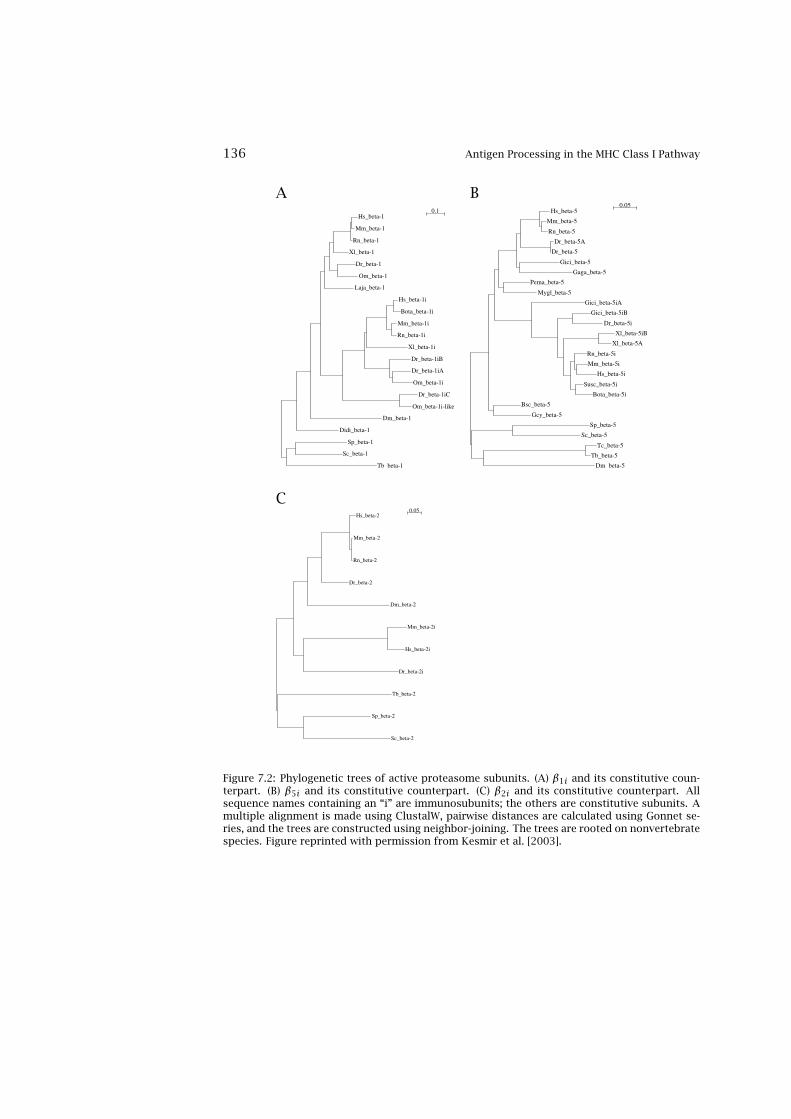
136 Antigen Processing in the MHC Class I Pathway
A B
Tb_beta-1
Sc_beta-1
Sp_beta-1
Didi_beta-1
Dm_beta-1
Om_beta-1i-like
Dr_beta-1iC
Om_beta-1i
Dr_beta-1iA
Dr_beta-1iB
Xl_beta-1i
Rn_beta-1i
Mm_beta-1i
Bota_beta-1i
Hs_beta-1i
Laja_beta-1
Om_beta-1
Dr_beta-1
Xl_beta-1
Rn_beta-1
Mm_beta-1
Hs_beta-10.1
Dm_beta-5
Tb_beta-5
Tc_beta-5
Sc_beta-5
Sp_beta-5
Gcy_beta-5
Bsc_beta-5
Bota_beta-5i
Susc_beta-5i
Hs_beta-5i
Mm_beta-5i
Rn_beta-5i
Xl_beta-5A
Xl_beta-5iB
Dr_beta-5i
Gici_beta-5iB
Gici_beta-5iA
Mygl_beta-5
Pema_beta-5
Gaga_beta-5
Gici_beta-5
Dr_beta-5
Dr_beta-5A
Rn_beta-5
Mm_beta-5
Hs_beta-50.05
C
Sc_beta-2
Sp_beta-2
Tb_beta-2
Dr_beta-2i
Hs_beta-2i
Mm_beta-2i
Dm_beta-2
Dr_beta-2
Rn_beta-2
Mm_beta-2
Hs_beta-20.05
Figure 7.2: Phylogenetic trees of active proteasome subunits. (A) β1i and its constitutive coun-terpart. (B) β5i and its constitutive counterpart. (C) β2i and its constitutive counterpart. Allsequence names containing an “i” are immunosubunits; the others are constitutive subunits. Amultiple alignment is made using ClustalW, pairwise distances are calculated using Gonnet se-ries, and the trees are constructed using neighbor-joining. The trees are rooted on nonvertebratespecies. Figure reprinted with permission from Kesmir et al. [2003].

Specificity of the (Immuno)Proteasome 137
subunit dn dn/ds subunit dn dn/ds subunit dn dn/dsα-1 0.287 0.006 β-1 0.400 0.083 β-1i 0.992 0.164α-2 0.351 0.012 β-2 0.373 0.105 β-2i 0.660 0.138α-3 0.447 0.011 β-3 0.391 0.048α-4 0.406 0.021 β-4 0.257 0.098α-5 0.252 0.028 β-5 0.398 0.119 β-5i 0.489 0.186α-6 0.327 0.090 β-6 0.581 0.106α-7 0.362 0.039 β-7 0.432 0.075MHC 0.049 1.418phosphatase 6 0.359 0.004
Table 7.1: dn/ds ratio of different proteasome subunits from mice and men. Only the subunitsβ-1, β-2, and β-5 and their immuno counterparts are active. For comparison, the dn/ds ratiois also calculated for a housekeeping gene, phosphatase subunit 6 (NM_002721 and BC002223),and two MHC class I molecules, HLA-A*02011 (HLA00005) and HLA-A*01011 (HLA00001) fromthe IMGT/HLA (imgt.cines.fr) [Robinson et al., 2001] database.
1.0 (see table 7.1). Thus, the immunosubunits are indeed coded for in muta-tional hotspots (i.e., in the MHC class II region). However, all immunosubunitsalso have higher dn/ds ratios than their constitutive counterparts (see table7.1), suggesting that the immunosubunits are evolving faster. The subunitsthat do not have enzymatic activity have lower dn/ds ratios. The immunosub-units are nevertheless not the fastest evolving molecules involved in antigenprocessing and presentation; MHC molecules evolve even faster ([Tanaka andNei, 1989, Hughes and Nei, 1988, 1989]; see table 7.1). In summary, this typeof phylogenetic analysis points to a functional differentiation between the im-munoproteasome and the constitutive proteasome.
7.3 Specificity of the (Immuno)Proteasome
The specificity of the proteasome is often studied by in vitro experiments.One example of such an experimental system is the one of Toes et al. [2001],who studied the differences between immunoproteasome and constitutive pro-teasome specificity. Toes et al. [2001] calculated the frequency distributionsof amino acids at cleavage sites and their flanking regions. The cleavage oc-curs between the P1 and the P1′ position [Berger and Schechter, 1970]. Theresidues on the left flanking region of the cleavage are called P1, P2, P3, P4,. . ., while the right side is referred to as P1′, P2′, . . . It has been suggested thatthe P1 position is the most important position determining cleavage [Altuviaand Margalit, 2000], although the flanking region may also be important [Moet al., 2000, Beekman et al., 2000, Ossendorp et al., 1996]. One way of ana-lyzing such data is to calculate the information content at the cleavage siteand in the region flanking the cleavage site. We use two different informationmeasures. The first one is the Shannon information (as described in section

138 Antigen Processing in the MHC Class I Pathway
4.2.1). The second information measure is the Kullback-Leibler information,which identifies by how much the observed distribution differs from the back-ground distribution (see section 4.2.2). In other words this measure correctsthe information content for the distribution of amino acids in natural proteins.
The information content for the P1 position in the immunoproteasomedigests is much higher than in the constitutive proteasome digests (figure7.3a,b). In other words, cleavage by the immunoproteasome is restricted tofewer amino acids, whereas the constitutive proteasome is more degenerate,i.e., many different amino acids can be used as potential cleavage sites. Thus,these results suggest that the immunoproteasome is more specific than theconstitutive proteasome. Another measure for comparing the specificity ofthe two forms of the proteasome is the diversity of amino acids present at theP1 position, as defined in terms of the Simpson index. We define the diversityat position i in an alignment as D(i) = 1/SI(i), where SI(i) is the Simpson in-dex, SI(i) =
∑aa (paa(i))2, and the probabilities satisfy
∑aa paa(i) = 1. This
diversity measure yields a value between 1 and 20; the higher the diversitythe more degenerate the proteasome (i.e., 20 means that all amino acids areused with equal frequency at a given position, and 1 means that only a sin-gle amino acid is found at a given position). The diversity of the P1 positionof the immunoproteasome digests is 5.83, and that of the constitutive pro-teasome is 9.53 (figure 7.3c), again suggesting that the immunoproteasome ismore specific.
We can repeat the analysis without taking into account the frequency withwhich fragments are produced, i.e., we can only look at the observed cleavagesites. The result of the analysis is shown in figure 7.3(d-f). According to thecleavage maps reported in Toes et al. [2001], out of 436 residues in enolase,55 sites are used by the immunoproteasome only, 73 by the constitutive pro-teasome only, and 69 by both proteasomes. In other words, the fraction ofsites used by the immunoproteasome is (55+ 69)/436 = 0.28 and by the con-stitutive proteasome, (73+ 69)/436 = 0.33. The expected value of the overlapthen becomes 0.28× 0.33× 436 = 40 sites, i.e., the observed overlap is largerthan the expected value. The large overlap was also observed in a independentstudy [Peters et al., 2002]. The 55 sites used exclusively by the immunoprotea-some are clearly more specific than the 73 sites used only by the constitutiveproteasome as demonstrated by the high information content, and by the lowdiversity at the P1, P2, and P5′ positions used by the immunoproteasome (seefigure 7.3d-f).
In figure 7.3d-f, the Kullback-Leibler information is much lower than theShannon information for the cleavage sites that are used by both proteasomes.This means that the overlapping sites consist mainly of frequent amino acidsthat do not carry much information, i.e., the overlapping sites are not veryspecific. The sites used only by the constitutive proteasome contain hardly

Specificity of the (Immuno)Proteasome 139
Figure 7.3: Information content and diversity at and around the cleavage sites of the immuno-proteasome (filled circles), and the constitutive proteasome (open circles). In panels (d-f) theobserved cleavage sites used only by the immunoproteasome are given by filled circles, whileopen circles represent sites used only by the constitutive proteasome, and filled diamonds byboth. The figure is generated using the frequency data (a-c) and the cleavage maps (d-f) of Toeset al. [2001]. Panels (a) and (d) represent the Shannon information, panels (b) and (e) representthe Kullback-Leibler information, and panels (c) and (f) represent diversity. Cleavage nomencla-ture according to Berger and Schechter [1970]. Figure adopted from Kesmir et al. [2003].
any motifs, which is indicated by the low information content and the highdiversity of amino acid usage. This suggests that the constitutive proteasomeuses semispecific and degenerate sequence signals to cleave a protein.
The two proteasomes are also differentiated on the basis of the preferredamino acids at the P1 position. In figure 7.4 the distribution of amino acids atthe P1 position is shown. The constitutive proteasome seems to use the acidicamino acids D and E more than one might expect from their distributions inthe enolase protein. In the sequence logo of the P1 position of the immunopro-

140 Antigen Processing in the MHC Class I Pathway
Figure 7.4: Sequence logo at P1 position of all digested fragments found by Toes et al. [2001].This sequence logo has been corrected for the fact that some amino acids are found frequentlyor rarely in the enolase protein, i.e., it is based on Kullback-Leibler information. I-P1 is the P1position of the immunoproteasome digests, C-P1 stands for the P1 position of the constitutiveproteasome digests, and IC-P1 are the P1 positions used by both forms of proteasome. Figureadopted from Kesmir et al. [2003]. See plate 10 for color version.
teasome (figure 7.4), D and E are hardly visible. Thus, the immunoproteasomemakes considerably less use of the acidic amino acids than does the constitu-tive proteasome [Cardozo and Kohanski, 1998, Eleuteri et al., 1997].
Since all these results suggest that the immunoproteasome is a more spe-cific enzyme complex, one would expect the immunoproteasome to use fewercleavage sites in a given protein. Therefore, it is remarkable that when enolasewas degraded with immunoproteasomes and constitutive proteasomes, ap-proximately the same number of cleavage sites were observed (similar resultswere obtained for degradation of ovalbumin [Cascio et al., 2001]). One reasonfor this is that the immunoproteasome uses leucine, which is a very abundantamino acid, much more frequently than the constitutive proteasome. There-fore, the immunoproteasome seems to be able to degrade proteins efficientlydespite its increased specificity and as a result of this the replacement of theconstitutive subunits by immunosubunits does not inhibit cellular growth orviability [Groettrup et al., 2001]. This is important since the cells expressingthe immunoproteasome transiently, or for longer periods, need to maintainthe necessary housekeeping operations.

Predicting Proteasome Specificity 141
7.4 Predicting Proteasome Specificity
Successful prediction of the proteasome cleavage site specificity should bevaluable in the design of treatments based on CTL responses. For example,prediction could help in the choice of peptides for use in the treatment of CTL-mediated autoimmune diseases, or in vaccines inducing T cell–mediated im-munity. However, the complexity of proteasomal enzymatic specificity makessuch predictions difficult.
We will here mention some of the major proteasomal cleavage predic-tion methods. The first method, FragPredict, was developed by Holzhutteret al. [1999] and is publicly available as a part of MAPPP service (www.mpiib-berlin.mpg.de/MAPPP/), which combines proteasomal cleavage prediction withMHC and TAP binding prediction. FragPredict consists of two algorithms. Thefirst algorithm uses a statistical analysis of cleavage-enhancing and -inhibitingamino acid motifs to predict potential proteasomal cleavage sites [Holzhutteret al., 1999]. The second algorithm, which uses the results of the first algo-rithm as an input, predicts which fragments are most likely to be generated.This model takes the time-dependent degradation into account based on akinetic model of the 20S proteasome [Holzhutter and Kloetzel, 2000]. At themoment, FragPredict is the only method that can predict fragments, insteadof only possible cleavage sites.
PAProC (www.paproc.de) is a prediction method for cleavages by human aswell as wild-type and mutant yeast proteasomes. The influences of differentamino acids at different positions are determined by using a stochastic hill-climbing algorithm [Kuttler et al., 2000] based on the experimentally in vitroverified cleavage and noncleavage sites [Nussbaum et al., 2001].
Both methods make use of limited in vitro data. Moreover, FragPredict isa linear method, and it may not capture the nonlinear features of the speci-ficity of the proteasome. However, another prediction system exists, NetChop[Kesmir et al., 2002], which has two extensions: first, the prediction system istrained on multilayered neural networks using in vitro degradation data. Thistechnique is more powerful than PAProC, which uses a one-layered network topredict proteasome cleavage. Second, the approach uses naturally processedMHC class I ligands to predict proteasomal cleavage. Since some of these lig-ands are generated by immunoproteasomes and some by the constitutive pro-teasome, such a method should predict the combined specificity of both formsof proteasomes.
The data used to train NetChop stem from two different sources: The firstset (MHC ligands) comprises 458 cleavage sites determined by MHC class I lig-ands of 188 human proteins [Altuvia and Margalit, 2000]. The distribution ofamino acid residues around the cleavage site for this data set is shown in logoform in figure 7.5. The MHC ligand region is shown as dotted positions. Note

142 Antigen Processing in the MHC Class I Pathway
Figure 7.5: Sequence logo of N- and C-terminal cleavage sites for the MHC ligand database(229 unique sites for both terminals); cleavage nomenclature according to Berger and Schechter[1970]. The level of conservation at each position is computed as the Kullback-Leibler infor-mation content. The dotted positions correspond to the MHC class I ligand. The informationcontent around the C-terminal is much higher than that around the N-terminal. Note that theP1 position for C-termini is the last position of the MHC class I ligand. Figure reprinted withpermission from Kesmir et al. [2002]. See plate 11 for color version.
that the C-terminal cleavage site (i.e., the P1 position; cleavage nomenclatureaccording to Berger and Schechter [1970]) is included in the MHC ligand. InKullback-Leibler sequence logos amino acid symbols are scaled according totheir frequencies of occurrence relative to the background distribution. Thatis, if an amino acid is overrepresented, it will get a large height. On the otherhand, if it is underrepresented, it will also receive a large height, but will begiven a negative value so that it can be visualized differently, e.g., as an upside-down letter. If it occurs at nearly the same frequency as the background distri-bution, it will have a very small height. In generating this logo, the amino acidfrequencies within the MHC ligand (excluding the last position) were used tofind the background distribution, i.e., the distribution of the amino acids thatare not cleaved.
The information content is much higher around the C-terminal thanN-terminal, as previously reported by Altuvia and Margalit [2000]. This isprobably due to the involvement of other proteolytic processes on generatingthe N-terminal of MHC class I ligands [Mo et al., 1999, Stoltze et al., 2000b].

Predicting Proteasome Specificity 143
Figure 7.6: Sequence logo generated using in vitro data on digestion of enolase and β-casein byhuman 20S constitutive proteasome. To create this logo, 156 distinct cleavage sites were used.Figure reprinted with permission from Kesmir et al. [2002]. See plate 12 for color version.
The second data set contains in vitro degradation data by human 20S con-stitutive proteasome for two proteins: enolase [Toes et al., 2001], and β-casein[Emmerich et al., 2000]. A sequence logo based on 184 distinct sites fromthese two proteins is shown in figure 7.6. Here the most significant position isthe P1 residue, followed by P2′, P2, and P3. The dominance of the hydropho-bic residues (L, V, A) together with the acidic ones (D, E) at these positionsis clear, whereas P seems to inhibit cleavage. Comparison of figures 7.5 and7.6 suggests that the nature of the in vitro degradation data is different fromMHC class I ligands. This can be due to the involvement of the immunoprotea-some in generation of MHC class I ligands. However, a clear conclusion cannotbe made here, because the sequence logo displayed in figure 7.5 is indeed acombination of the proteasomal, TAP, and MHC specificities.
Sequence features used for discrimination by the network can be extractedby inspecting the weights of individual neurons. In order to enlarge the anal-ysis of cleavage-promoting and -inhibiting motifs, the weights of a linear net-work trained on the constitutive proteasome data can be analyzed. In the P1position large hydrophobic residues (F, L, and polar Y) promote cleavage pre-diction by the network. Proline at P1 and P2 is strictly cleavage-inhibiting,
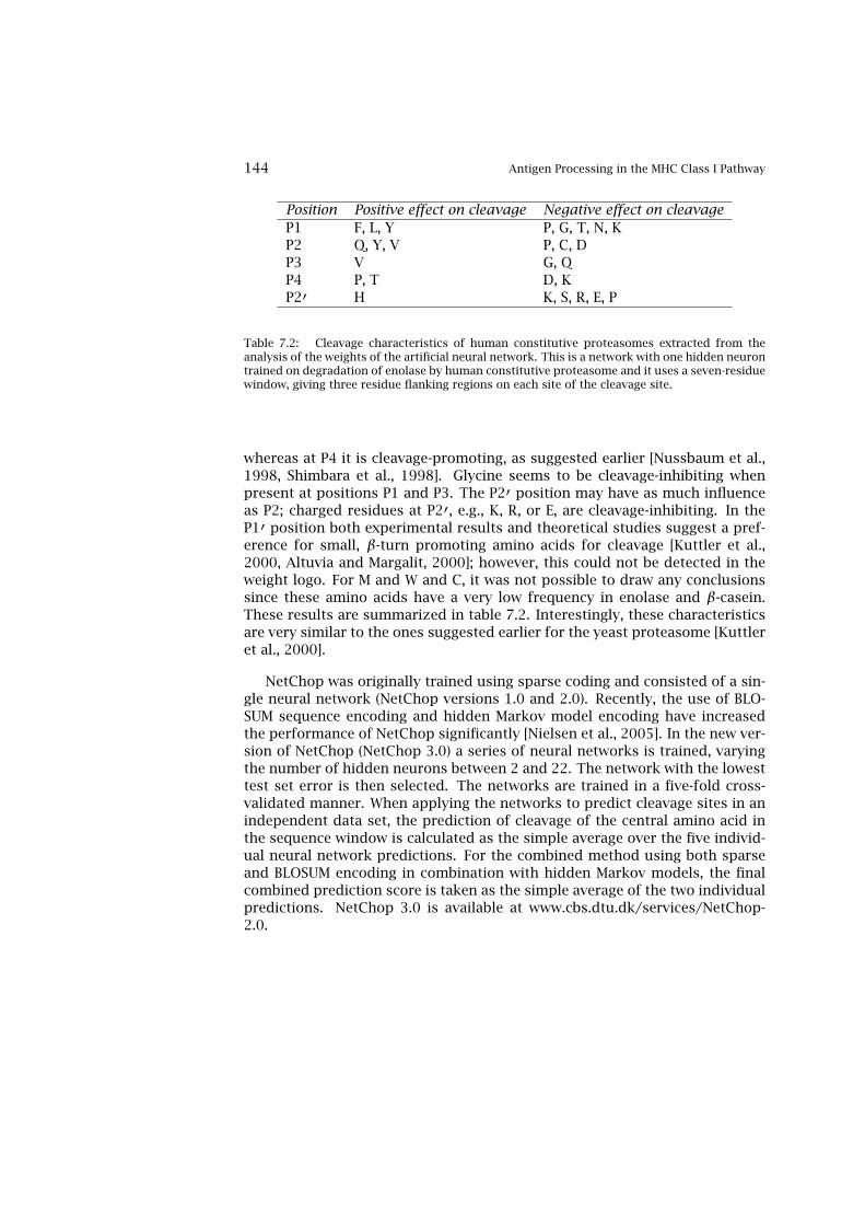
144 Antigen Processing in the MHC Class I Pathway
Position Positive effect on cleavage Negative effect on cleavageP1 F, L, Y P, G, T, N, KP2 Q, Y, V P, C, DP3 V G, QP4 P, T D, KP2′ H K, S, R, E, P
Table 7.2: Cleavage characteristics of human constitutive proteasomes extracted from theanalysis of the weights of the artificial neural network. This is a network with one hidden neurontrained on degradation of enolase by human constitutive proteasome and it uses a seven-residuewindow, giving three residue flanking regions on each site of the cleavage site.
whereas at P4 it is cleavage-promoting, as suggested earlier [Nussbaum et al.,1998, Shimbara et al., 1998]. Glycine seems to be cleavage-inhibiting whenpresent at positions P1 and P3. The P2′ position may have as much influenceas P2; charged residues at P2′, e.g., K, R, or E, are cleavage-inhibiting. In theP1′ position both experimental results and theoretical studies suggest a pref-erence for small, β-turn promoting amino acids for cleavage [Kuttler et al.,2000, Altuvia and Margalit, 2000]; however, this could not be detected in theweight logo. For M and W and C, it was not possible to draw any conclusionssince these amino acids have a very low frequency in enolase and β-casein.These results are summarized in table 7.2. Interestingly, these characteristicsare very similar to the ones suggested earlier for the yeast proteasome [Kuttleret al., 2000].
NetChop was originally trained using sparse coding and consisted of a sin-gle neural network (NetChop versions 1.0 and 2.0). Recently, the use of BLO-SUM sequence encoding and hidden Markov model encoding have increasedthe performance of NetChop significantly [Nielsen et al., 2005]. In the new ver-sion of NetChop (NetChop 3.0) a series of neural networks is trained, varyingthe number of hidden neurons between 2 and 22. The network with the lowesttest set error is then selected. The networks are trained in a five-fold cross-validated manner. When applying the networks to predict cleavage sites in anindependent data set, the prediction of cleavage of the central amino acid inthe sequence window is calculated as the simple average over the five individ-ual neural network predictions. For the combined method using both sparseand BLOSUM encoding in combination with hidden Markov models, the finalcombined prediction score is taken as the simple average of the two individualpredictions. NetChop 3.0 is available at www.cbs.dtu.dk/services/NetChop-2.0.

Comparison of Proteasomal Prediction Performance 145
7.5 Comparison of Proteasomal Prediction Performance
To compare the performance of the three publicly available methods, all themethods above were tested on a set of MHC class I ligands publicly available[Saxova et al., 2003, Nielsen et al., 2005]. In the test the ability of the methods(1) to predict correctly the C-terminal of a ligand and (2) not to predict majorcleavage sites within the ligand was investigated. N-terminal cleavage analysiswas excluded, because the majority of T cell epitopes are trimmed on their N-terminal by other peptidases, e.g., in endoplasmic reticulum [Mo et al., 1999].
The comparison of the predictive performance of FragPredict, PAProC,NetChop 2.0, and NetChop 3.0 is given in figure 7.7. To address the ques-tion of whether the difference in predictive performance between differentprediction methods is statistically significant, a bootstrap experiment can beperformed [Press et al., 1992]. In the bootstrap experiment, a series of N dataset replicas is generated by randomly drawing n data points with replacementfrom the original data set, where n is the size of the original data set. For eachdata set, the predictive performance of two methods is then evaluated. Thep-value for the hypothesis that method M1 performs better than method M2is then estimated from the simple ratio (M1 > M2)/N, where (M1 > M2) isthe number of experiments where method M1 outperformed method M2, andN the number of bootstrap replicas. A p-value greater than .95 will indicatethat the one method significantly outperforms the other.
Performing the bootstrap experiment comparing the Matthews correlationcoefficient values, it was found that the new method (NetChop 3.0) had a per-formance that is significantly higher than that of NetChop 2.0 (p < .001). Thereare two reasons for the increase in predictive performance. First of all, thenetwork training strategy differs between NetChop 2.0 and NetChop 3.0. Inthe latter we perform a fivefold cross-validated training, where each networktraining is stopped when the test set error is minimal. This strategy leads toan ensemble of five networks each with an individual prediction bias. In thetraining of NetChop 2.0, the fivefold training was performed to estimate opti-mal parameter settings and the final NetChop 2.0 network is a single networktrained on all data using these optimal parameter settings. In a separate ex-periment it was found that use of network ensemble alone can increase theperformance of NetChop 2.0 significantly (p < .003). Thus, it is clear that thestrategy of generating a network ensemble leads to a higher predictive perfor-mance.
The second difference between NetChop 2.0 and NetChop3.0 is the use ofdifferent sequence encoding schemes; BLOSUM encoding and the informationcoming from the hidden Markov model leads to an increase in performance.The gain in sensitivity of NetChop3.0 over that of NetChop 2.0 is 0.07 (0.81-0.74), and is achieved at a constant or slightly increased specificity (0.46 vs.

146 Antigen Processing in the MHC Class I Pathway
Figure 7.7: Benchmark calculation of cleavage predictions for neural network methods trainedon MHC ligand data and evaluated on 231 MHC ligands. The performance values for FragPredict,PAProC, and NetChop2.0 are taken from Saxova et al. [2003]. NetChop3.0 refers to a combina-tion of two neural network ensembles trained using sparse and BLOSUM encoding in combina-tion with the hidden Markov model, respectively. The performance measures are calculated asdescribed in chapter 4. CC is the Matthews correlation coefficient [Nielsen et al., 2005].
0.42 for NetChop 3.0 and NetChop 2.0 methods, respectively). The gain in sen-sitivity means that the combined neural network method can correctly iden-tify close to 10% more cleavage sites than NetChop 2.0 with no increase in thefalse-positive rate. The increase in performance is also visible in the correla-tion coefficient (CC) values: CC is 0.16 for NetChop 2.0 and 0.28 for NetChop3.0.
A new version of the NetChop20S neural network (based on in vitro dataonly) using the new network training strategy and sequence encoding schemeswas also trained [Nielsen et al., 2005]. In figure 7.8, we compare the predic-tive performance in terms of a ROC curve for the two prediction methods,NetChop20S and NetChop20S-3.0. One important difference between the pre-dictive performance of NetChop20S-3.0 and that of NetChop20S is the largeincrease in sensitivity (correctly predicted cleavage sites proportion) at lowvalue of the false-positive proportion. At a false-positive rate of 0.1 the sensi-tivity of NetChop20S method is 0.43, corresponding to a correct identificationof only 26 of the 61 cleavage sites. For NetChop20S-3.0 the corresponding sen-sitivity value is 0.57, and the number of correctly identified cleavage sites isthus 35. Thus the combination of many neural networks trained on differenttypes and combinations of sequence encodings leads to more accurate predic-

Escape from Proteasomal Cleavage 147
0.0 0.2 0.4 0.6 0.8 1.0False positive proportion (1-specificity)
0.0
0.2
0.4
0.6
0.8
1.0
Tru
e po
sitiv
e pr
opor
tion
(sen
sitiv
ity) NetChop20S-3.0
Netchop20S
0.00 0.05 0.10 0.15 0.20 0.250.0
0.2
0.4
0.6
Figure 7.8: ROC curves comparing the predictive performance of the combined NetChop20S-3.0 method and NetChop20S. The curves are calculated using the bootstrap method and areaveraged over 1000 bootstrap replicas. The corresponding AROC values are 0.85 and 0.81 forthe combined and NetChop20S methods, respectively. The insert to the graph shows the high-specificity part of the ROC curve in detail. Reprinted with permission from Nielsen et al. [2005].
tion algorithms, i.e., one can obtain an increase in the prediction sensitivitywithout a loss in the specificity. These results are in agreement with stud-ies showing that the combined approach improves the prediction accuracy ofMHC binding (see chapter 6 and [Nielsen et al., 2003]). This new version ofNetChop (NetChop 3.0) is available at www.cbs.dtu.dk/services/NetChop-3.0.
7.6 Escape from Proteasomal Cleavage
The CTL response often causes a strong selection pressure on pathogens, forc-ing these microorganisms to develop different ways to evade the response.These evasions include point mutations or insertions/deletions in the proteinsequences that disturb (1) peptide binding of MHC molecules, (2) binding of Tcell receptor to peptide-MHC complex, and (3) processing of the peptide. Fornow we will focus on evasion from proteasomal processing.
Mutations that influence epitope processing are critical, as cases of immuneescape due to mutations in an epitope’s flanking regions have demonstratedthat escape through processing abrogation is of immunological significance[Beekman et al., 2000, Chassin et al., 1999, Goulder et al., 1997]. Cleavagesites generated by the immunoproteasome are sensitive to the surrounding
148 Antigen Processing in the MHC Class I Pathway
sequence [Niedermann et al., 1999], although no simple cleavage signal is ap-parent. We took HIV as a model pathogen to study whether it is evolving toprevent cleavage [Yusim et al., 2002]. The majority of HIV CTL escape andcross-reactivity studies focus on the influence of substitutions within an epi-tope, that would influence only class I HLA and T cell receptor (TCR) interac-tions by testing of synthetic peptide variants for cross-reactivity in vitro [Caoet al., 1997]. Thus the relative influence of processing escape mutations is notwell addressed in the HIV literature.
To analyze the evolution of HIV sequences with respect to proteasomalcleavage, we can use NetChop 2.0 [Yusim et al., 2002]. NetChop 2.0 was usedto predict cleavage at every site of each sequence in the alignment. Sincewe are interested in learning about the tendency of a site to be cleaved at thepopulation level, we considered the distributions of prediction scores obtainedfor each position from all sequences in the full alignment. The median valueof predictions over all sequences obtained for each site in each HIV-1 proteinalignment was used to represent the population cleavage prediction score forthe site.
The median prediction scores at true C-terminals of experimentally ob-served HIV epitopes vs. all other remaining sites, and vs. only sites fromepitope-lacking regions, were found to be statistically significantly higher us-ing a Mann-Whitney test, for each of the five proteins studied (figure 7.9).NetChop predictions are of course imperfect; a particular site might be mis-classified. The highly significant correlation shown in figure 7.9, betweenC-terminals of identified CTL epitopes and conservation of predicted cleav-age sites in an alignment of HIV proteins shows that at the population level (asopposed to just a single strain), NetChop can distinguish classes of positionsthat are favorable for cleavage, and positions that are embedded in a contextthat makes cleavage very unlikely. Regional localization of low NetChop scoresin areas where there are no defined CTL epitopes suggests that these proteinsubregions may have reduced epitope processing potential, and that this fea-ture can persist throughout the HIV-1 M group.
7.7 Post-Proteasomal Processing of Epitopes
The C-terminals of CTL epitopes are generated precisely by the proteasomeand no further trimming is needed [Cascio et al., 2001]. An exact N-terminalcleavage is, however, less essential since a precursor peptide may be trimmedat the N-terminal by other peptidases in the cytosol [Levy et al., 2002, Reitset al., 2003] and after TAP transport into the ER by peptidases while it bindsto the MHC class I molecule [Serwold et al., 2002, York et al., 2002, Saric et al.,2002]. To investigate the extent of N-terminal trimming of CTL epitopes, we

Post-Proteasomal Processing of Epitopes 149
Figure 7.9: For each protein and for each sequence in the alignment, site-specific predictionscores were computed with NetChop (www.cbs.dtu.dk/Services/NetChop). Then for each siteof the alignment the site-specific predictions were calculated as the medians of the predictionsfrom all protein sequences in the alignment. Site-specific predictions were then organized intofour groups for each protein: group 1, denoted as “C-term” in the figure, represents the predic-tion scores at the sites corresponding to known C-terminals of experimentally defined epitopes;group 2, denoted as “No Epitopes,” represents the predictions at all sites taken from epitope-lacking regions; and group 3, denoted as “No C-term,” refers to the predictions at all sites whichdo not serve as C-terminals of experimentally observed HIV epitopes. The bars in the figure showthe medians of the distributions for each group for each protein. The lines overlapping eachbar correspond to the 25th and 75th percentiles of the distributions. Using the nonparametricMann-Whitney test, the scores for known C-terminal positions, “C-term,” were compared to thegroups “No Epitope” and “No C-term.” For all five proteins the prediction scores at C-terminalsof all experimentally observed HIV epitopes were found to be statistically significantly higherthan prediction scores in the epitope-poor regions (p24: p = .002; Nef: p = .002; p17: p = .002;RT: p < .0001; Env: p < .0001) and positions that are not C-terminals of experimental epitopes(p24: p = .007; Nef: p = .001; p17: p = .001; RT: p < .0001; Env: p < .0001). A differ-ent strategy for training NetChop to recognize cleavage sites, based on relative frequency ofcleavage events in vitro observed in the enolase and β-casein proteins rather than known epi-topes (NetChop-20S), gave a statistically significant difference in the prediction scores betweenC-terminal positions and epitope-lacking regions for Env (p = .0012) and P24 (p = .0006), atrend for RT (p = .08), but not for p17 (p = .67), and Nef (p = .67). Figure adopted from Yusimet al. [2002].
used NetChop predictions. In a large set of CTL epitopes (as used to comparedifferent proteasomal prediction methods), we identified the source proteinof each epitope and extracted those protein sequences from Swiss-Prot. Weestimate the N-terminal extension as the distance from the N-terminal of theepitope to the nearest cleavage site (prediction value > 0.5) at the same side(i.e., we are not normalizing the natural epitope length to define the exten-sion). The output from the neural network is related to the probability of a
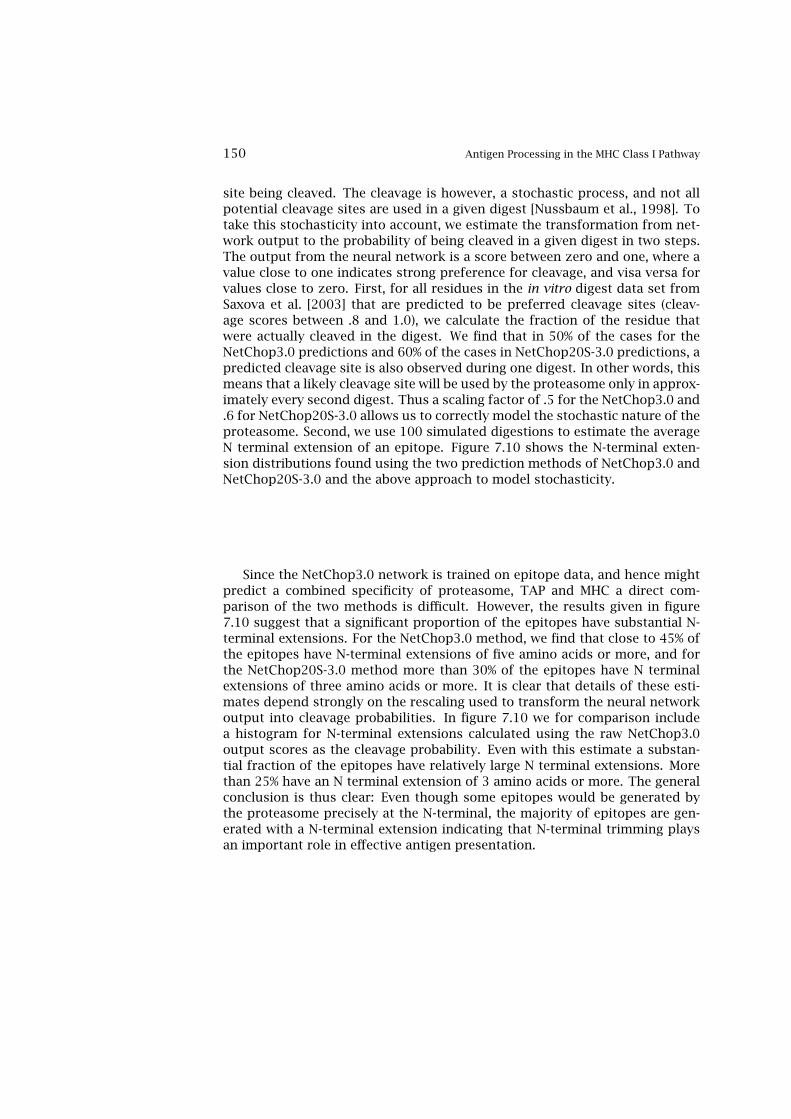
150 Antigen Processing in the MHC Class I Pathway
site being cleaved. The cleavage is however, a stochastic process, and not allpotential cleavage sites are used in a given digest [Nussbaum et al., 1998]. Totake this stochasticity into account, we estimate the transformation from net-work output to the probability of being cleaved in a given digest in two steps.The output from the neural network is a score between zero and one, where avalue close to one indicates strong preference for cleavage, and visa versa forvalues close to zero. First, for all residues in the in vitro digest data set fromSaxova et al. [2003] that are predicted to be preferred cleavage sites (cleav-age scores between .8 and 1.0), we calculate the fraction of the residue thatwere actually cleaved in the digest. We find that in 50% of the cases for theNetChop3.0 predictions and 60% of the cases in NetChop20S-3.0 predictions, apredicted cleavage site is also observed during one digest. In other words, thismeans that a likely cleavage site will be used by the proteasome only in approx-imately every second digest. Thus a scaling factor of .5 for the NetChop3.0 and.6 for NetChop20S-3.0 allows us to correctly model the stochastic nature of theproteasome. Second, we use 100 simulated digestions to estimate the averageN terminal extension of an epitope. Figure 7.10 shows the N-terminal exten-sion distributions found using the two prediction methods of NetChop3.0 andNetChop20S-3.0 and the above approach to model stochasticity.
Since the NetChop3.0 network is trained on epitope data, and hence mightpredict a combined specificity of proteasome, TAP and MHC a direct com-parison of the two methods is difficult. However, the results given in figure7.10 suggest that a significant proportion of the epitopes have substantial N-terminal extensions. For the NetChop3.0 method, we find that close to 45% ofthe epitopes have N-terminal extensions of five amino acids or more, and forthe NetChop20S-3.0 method more than 30% of the epitopes have N terminalextensions of three amino acids or more. It is clear that details of these esti-mates depend strongly on the rescaling used to transform the neural networkoutput into cleavage probabilities. In figure 7.10 we for comparison includea histogram for N-terminal extensions calculated using the raw NetChop3.0output scores as the cleavage probability. Even with this estimate a substan-tial fraction of the epitopes have relatively large N terminal extensions. Morethan 25% have an N terminal extension of 3 amino acids or more. The generalconclusion is thus clear: Even though some epitopes would be generated bythe proteasome precisely at the N-terminal, the majority of epitopes are gen-erated with a N-terminal extension indicating that N-terminal trimming playsan important role in effective antigen presentation.

Predicting the Specificity of TAP 151
Figure 7.10: Distribution of N-terminal extensions for the 231 epitopes in the Saxová benchmarkdata set. The N-terminal extension is calculated as the distance to the nearest cleavage site at theN terminal side of the epitope. The stochastic nature of the proteasomal cleavage is estimatedfrom the network output score as described in the text. The filled and dashed bars show the N-terminal extensions predicted using the NetChop3.0 and NetChop20S-3.0 methods, respectivelyand correcting the predictions for stochasticity. The open bars show the N-terminal extensionspredicted using the raw NetChop3.0 output [Nielsen et al., 2005].
7.8 Predicting the Specificity of TAP
Transport of the peptides into the ER is an essential step in the MHC class Ipresentation pathway. This task is done by TAP molecules that are encoded bythe MHC. TAP belongs to the ABC family of ATP-dependent transporters, andcomprises two transmembrane chains, TAP1 and TAP2. Different species havedifferent degrees of TAP polymorphism: while there is hardly any functionalTAP polymorphism found among humans, the rat has clearly two distinct TAPalleles [Joly and Butcher, 1998].
Peptide and ATP binding result in conformational changes [Reits et al.,2000]. Following an initial peptide binding step (probably very fast), ATP hy-drolysis induces pore opening and disrupts peptide binding. The peptide isreleased from the altered peptide binding site and is translocated through theopen pore to the ER. This translocation occurs via simple diffusion. Later the

152 Antigen Processing in the MHC Class I Pathway
pore closes, and the peptide binding domain returns to the original conforma-tion, completing the translocation cycle.
Peptides that are 8 to16 amino acids long are good substrates for TAP, but9 to 12 amino acid fragments seem to be the best [Uebel and Tampe, 1999].The C-terminals of the good substrates are mainly hydrophobic, while acidicamino acids are strongly disfavored. In addition to the C-terminal, the firstthree residues in the N-terminal seems to be important. In the first two posi-tions basic residues are favored, while the third position can be either a tryp-tophan or tyrosine. Proline at position 2is the strongest single destabilizingresidue found, nearly completely abolishing the binding [Uebel et al., 1997].The binding motif of the TAP, especially in the C-terminal, resembles closelythe binding motifs of many human MHC molecules.
Relatively few methods have been developed to predict the specificity ofTAP. Daniel et al. [1998] have developed artificial neural networks using 9merswhere TAP binding affinity was determined experimentally. Surprisingly, theyfound that some MHC alleles have ligands with very low TAP affinities, e.g.,HLA-A2. However, it has been shown that TAP ligands can be trimmed in ERbefore binding to MHC molecules (see above), i.e., a TAP ligand does not needto be 9 amino acids long. Thus, HLA-A2 might easily have precursors of itsoptimal ligands, which are also good TAP binders.
Recently, Peters et al. [2003a] used a stabilized matrix method to predictTAP affinity of peptides. This method has the advantage of not being bound toonly 9mers, but it can also be used for longer peptides. The method assumesthat only the first three positions in the N-terminal and the last position atthe C-terminal influences the TAP binding. The accuracy of this method ishigh, and the authors have shown that this method can be used to increasethe specificity of MHC binding predictions [Peters et al., 2003a].
With increasing numbers of TAP ligands available on the Internet (e.g., Jen-Pep database,www.jenner.ac.uk [Blythe et al., 2002]), it will likely soon be pos-sible to obtain more accurate TAP predictions.
7.9 Proteasome and TAP Evolution
It has recently been shown that the specificity of human MHC molecules hasevolved to fit the specificity of the immunoproteasome [Kesmir et al., 2003].Thus good MHC ligands also have a high probability to be generated by theproteasome. To add TAP to this evolutionary relation would increase the effi-cacy of the antigen processing and the presentation even further.
To investigate the footprints of a possible evolutionary fit between TAPand the proteasome specificities, we predict C-terminal cleavage for a set ofgood TAP ligands. TAP binding peptides were downloaded from the AntiJen

Proteasome and TAP Evolution 153
database (http://www.jenner.ac.uk/AntiJen/). This database contains a set ofclose to 350 unique peptides with known TAP binding affinity. Only 63 of thesepeptides are natural ligands with a “host” protein in the Swiss-Prot databaseand bind to TAP with an efficient affinity (i.e., affinity < 100,000 nM).
To quantify the similarity between TAP and proteasome specificity, we pre-dict C-terminal cleavage for the above-mentioned TAP ligands. We have shownthat our predictor trained on epitope data predicts the C terminal cleavage ofepitopes most correctly [Kesmir et al., 2002]. However, these networks mighthave learned the specificity of the TAP molecule, since TAP binding motifscould be embedded in the epitope data set. Therefore, we use the NetChop20S-3.0 predictor to circumvent a possible bias in the predictions. We predict theaverage C-terminal cleavage score of these “natural TAP ligands,” and com-pare that to the average cleavage score calculated in the set of natural TAPligands by shuffling the amino acids in the ligands. For the TAP ligands the av-erage cleavage score is 0.607±0.216, and for the shuffled ligand set the valueis 0.427±0.260. The average cleavage score in TAP ligand data set is signifi-cantly higher than for the shuffled ligands (p < .001 in a Student’s t-test for asignificantly different means [Press et al., 1992]). Thus, the TAP binding motif,especially the preference of C-terminal, allows for a significantly higher chanceof being cleaved by the proteasome. Note that our NetChop20S predictor istrained on the constitutive proteasome specificity. Since the immunoprotea-some specificity is much more adapted to TAP specificity [Nielsen et al., 2005],we expect that good TAP ligands be generated by the immunoproteasome morefrequently than our estimate here.
The TAP ligand data set we use contains many MHC ligands. Therefore,both analysis presented here might be showing actually the adaptation be-tween MHC molecules and the proteasome. To remove this bias, we predictcleavage of 500.000 9mers selected randomly from proteins in the Swiss-Protdatabase. In figure 7.11, we plot the average proteasomal cleavage score foreach of the 20 amino acids in this large peptide data set by the NetChop20S-3.0method versus the TAP preference score on the C terminal, which is adaptedfrom a method developed by [Peters et al., 2003a] to predict peptide bindingaffinity to human TAP molecules. A high proteasomal cleavage score indicatesa high chance of cleavage, and a low (negative) TAP score indicates a highchance of TAP transport. The TAP preference score and proteasomal cleav-age score is significantly correlated (Kendall’s τ = -0.44, p=0.007 [Press et al.,1992]). This correlation indicates that the TAP specificity to some degree isadapted so that, the peptides generated by the proteasome are transported ef-ficiently to the ER. While the correlation between the two scores is not perfect,hardly any amino acids are placed in the lower left part of the plot (only K ismarginally present in this part of the plot). This part of the plot contains aminoacids that are favored by TAP for transport but disfavored by proteasome for
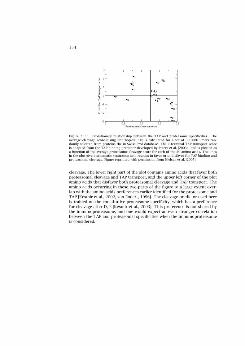
154 Antigen Processing in the MHC Class I Pathway
G
W
PK
N
T
S
C
HQA
I
E
V
D
M
L
FY
R
0 0.2 0.4 0.6 0.8Proteasomal cleavage score
-3
-2
-1
0
1
2
3
C te
rmin
al T
AP
tran
spor
t sco
re
Figure 7.11: Evolutionary relationship between the TAP and proteasome specificities. Theaverage cleavage score (using NetChop20S-3.0) is calculated for a set of 500,000 9mers ran-domly selected from proteins the in Swiss-Prot database. The C-terminal TAP transport scoreis adapted from the TAP binding predictor developed by Peters et al. [2003a] and is plotted asa function of the average proteasome cleavage score for each of the 20 amino acids. The linesin the plot give a schematic separation into regions in favor or in disfavor for TAP binding andproteasomal cleavage. Figure reprinted with permission from Nielsen et al. [2005].
cleavage. The lower right part of the plot contains amino acids that favor bothproteasomal cleavage and TAP transport, and the upper left corner of the plotamino acids that disfavor both proteasomal cleavage and TAP transport. Theamino acids occurring in these two parts of the figure to a large extent over-lap with the amino acids preferences earlier identified for the proteasome andTAP [Kesmir et al., 2002, van Endert, 1996]. The cleavage predictor used hereis trained on the constitutive proteasome specificity, which has a preferencefor cleavage after D, E [Kesmir et al., 2003]. This preference is not shared bythe immunoproteasome, and one would expect an even stronger correlationbetween the TAP and proteasomal specificities when the immunoproteasomeis considered.

Chapter 8
Prediction of Helper T Cell(MHC Class II) Epitopes
Only a small fraction of the possible peptides that is generated from proteinsof pathogenic organisms actually generate an immune response. The mostselective step in antigen presentation is the binding to the MHC molecule[Yewdell and Bennink, 1999]; thus prediction of which peptides that will binda specific MHC complex constitutes an important step in identifying potentialT cell epitopes suitable as vaccine candidates. The specificity of this bindingand that of some of the other processes involved in antigen presentation canbe predicted from the amino acid sequence, and such predictions can be usedto find and select epitopes for use in rational vaccine design and diagnostics.The aim is obviously also to increase the understanding of the role of the im-mune system in infectious diseases, autoimmune diseases, and cancers.
While MHC class I molecules mainly sample peptides from the cytosol,MHC class II samples peptides derived from endocytosed proteins. Unfoldedpolypeptides bind MHC class II molecules in the endocytic organelles (reviewedby Castellino et al. [1997]). Peptides presented by MHC class II molecules inturn activate CD4+ helper T lymphocytes (HTLs) to stimulate cellular and hu-moral immunity against the microorganisms.
Each of the MHC molecules has a different specificity, and the task of deriv-ing MHC prediction algorithms for all alleles is immense. However, many MHCalleles have very similar binding specificities, and it is therefore often possibleto find promiscuous peptides, which bind to a series of MHC variants. Thishas important implications, since it allows for high accuracy predictions forMHC alleles also in situations where the binding motif is poorly characterized[Brusic et al., 2002].
155

156 Prediction of MHC Class II epitopes
A B
Figure 8.1: Example of structure of peptide binding to MHC class II. (A) Cartoon representationof MHC class II showing that the overall structure of the complex is similar to MHC class Icomplexes (see figure 6.1). The bound peptide is shown in a sticks-representation. (B) MHC classII molecule shown on a molecular surface representation. It can be seen that the binding grooveis open in the ends in contrast to MHC class I. The figure is based on the PDB (www.rcsb.org/pdb)entry 1j8h. Figure Courtesy of Anne Mølgaard. See plate 13 for color version.
As opposed to MHC class I, the binding cleft of MHC class II molecules isopen-ended (figure 8.1), and allows the bound peptide to have significant “dan-gling ends.” As a result MHC class II binding peptides have a broad length dis-tribution complicating binding predictions. Thus identification of the correctalignment is a crucial part of identifying the core of an MHC class II bindingmotif. The MHC class II binding motifs have relatively weak and often degen-erate sequence signals. While some alleles like HLA-DRB1*0405 show a strongsignal for certain amino acids at the anchor positions, other alleles like HLA-DRB1*0401 allow basically all amino acids at all positions [Rammensee et al.,1999]. In this chapter, we describe how bioinformatics algorithms may be usedfor predicting MHC class II binding, using the so-called Gibbs motif sampler asan in-depth example.
8.1 Prediction Methods
Most of the work published on MHC class II ligand predictions has focusedon the HLA-DR alleles. Only a limited number of HLA-DQ and HLA-DP alleleshave been investigated. Godkin et al. [1998] have used eluted peptide sequencedata to characterize the binding motif of the HLA-DQ8, and HLA-DQ2 alleles.The HLA-DP molecules have scarcely been studied. Initially, they appeared
The Gibbs Sampler Method 157
less important in the immune response than HLA-DR and HLA-DQ molecules,because HLA-DP incompatibility did not seem to contribute to the risk of graft-vs.-host disease. However, it is now known that even a single mismatch canbe sufficient to trigger a specific T cell response after bone marrow transfer[Gaschet et al., 1996]. Castelli et al. [2002] use a biochemical binding assayfor the HLA-DP4 allele to verify binding of a set of synthetic peptides. Fromthe analysis they were able to characterize the amino acid preferences of theanchor positions.
For the HLA-DR alleles many different methods have been applied to pre-dict peptide-MHC binding, including simple binding motifs, quantitative ma-trices, hidden Markov models (HMMs), and artificial neural networks (ANNs).For class I these gap- and alignment-free methods can readily be applied sincethe binding motif is well characterized and most natural peptides that bindMHC class I are of close to equal length [Parker et al., 1994, Brusic et al., 1994,Rammensee et al., 1999, Buus et al., 2003, Nielsen et al., 2003]. However, thesituation for MHC class II binding is quite different due to the great variabilityin the length of natural MHC binding peptides. This length variability makesalignment a crucial part of predicting peptide binding. Quantitative matri-ces estimated from experimentally derived position-specific binding profileshave given reasonable performance in prediction of MHC class II binding [Setteet al., 1989a, Hammer et al., 1994, Marshall et al., 1995, Sturniolo et al., 1999].However, such matrices are very costly to derive and more importantly theylack the flexibility of data-driven machine-learning methods to be refined inan iterative manner when more data become available. Brusic et al. [1998b]have described a hybrid method for predicting peptide-MHC class II binding.They handle the alignment problem using an evolutionary algorithm and sub-sequently apply artificial neural networks to classify peptides as binding ornonbinding.
8.2 The Gibbs Sampler Method
The advanced motif sampler method [Nielsen et al., 2004] is based on the Gibbssampler method described by Lawrence et al. [1993]. Details of the method aregiven in chapter 4. The method attempts to find an optimal local alignmentof a set of N sequences by means of Monte Carlo Metropolis [Metropolis et al.,1953] sampling of the alignment space. In situations where the sequence pat-tern is very subtle and the motif is weak, this is a highly complex task, andconventional multiple sequence alignment programs will typically fail. In thefollowing, we describe an implementation of the Gibbs sampler method spe-cialized and optimized to locate and characterize the motif of MHC class I andclass II binding. The method applies the techniques of sequence weighting and
158 Prediction of MHC Class II epitopes
pseudocount correction for low counts as well as differential position-specificweighting and generation of consensus weight matrices to estimate the bind-ing motifs. A web server implementing the essential features of the Gibbssampler is available at http://www.cbs.dtu.dk/biotools/EasyGibbs/.
8.2.1 Gibbs Sampling
The algorithm samples possible alignments of a number of sequences, N. Foreach alignment a log-odds weight matrix is calculated as log(ppa/qa), whereppa is the frequency of amino acid a at position p in the alignment and qa isthe background frequency of that amino acid. The values of ppa are estimatedusing sequence weighting and pseudocount correction for low counts.
The fitness (energy) of a Gibbs-based alignment is calculated as theKullback-Leibler distance [Kullback and Leibler, 1951] between the observedamino acid distribution in a window and a background distribution,
E =∑p,aCpa log
ppaqa
, (8.1)
where Cpa is the occupancy number of amino acid a at position p in the align-ment. ppa and qa are as described above.
The set of possible alignments is, even for a small data set, very large. To al-low for an effective sampling of the alignment space the Monte Carlo Metropo-lis algorithm [Metropolis et al., 1953] is applied. The method implements asingle sequence and a phase shift Monte Carlo move. The probability of ac-cepting a move in the Monte Carlo sampling is defined using the conventionalMonte Carlo Metropolis relation P = min(1, edE/T ), where dE is the differencein energy between the end and start configurations and T a scalar. Details onthe implementation of the Gibbs sampler and the Monte Carlo moves are givenin chapter 4.
8.2.2 Weight-Matrix Calculation: The Parameters of the Gibbs Sam-pler
A central part of the motif sampler algorithm is the weight-matrix calculation,and the Gibbs sampler has a series of free parameters defining how a weightmatrix is calculated from a multiple alignment. The most important parame-ters are the
• sequence weighting method
• pseudocount correction method

The Gibbs Sampler Method 159
Supertype N Allele N NbindA1 92 HLA-A*0101 283 27A2 626 HLA-A*0204 528 144A3 228 HLA-A*0301 212 5B7 201 HLA-B*0702 154 24
Table 8.1: Data for the training and evaluation of the HLA class I binding predictions. The firstcolumn gives the supertype names included in the calculation, the second column the number ofunique 9mer peptides in the training set, the third column the HLA allele name for the evaluationset data, and the fourth and fifth columns the total number of peptides and the number ofbinders in the evaluation set, respectively. Binders were determined using a threshold of 500nM.
• weight on pseudocount correction
• position specific weighting.
The optimal settings of the parameters have to be determined first. Thiscan be done in a large-scale benchmark calculation using data sets where thealignment is not a question. For this purpose HLA class I binding peptidesare highly suitable. We know they contain a binding motif, and they are all ofnearly equal length so alignment will not be necessary.
Peptides known to bind MHC class I molecules are available from a num-ber of sources (see chapter 12). In this example they were extracted from thedatabases of SYFPEITHI and MHCPEP 1. To overcome the alignment issue, onlypeptides of length 9 were included. The peptides were clustered into the nineHLA supertypes (A1, A2, A3, A24, B7, B27, B44, B58, and B62) as described bySette and Sidney [1999]. These peptides constitute the training set for the MHCclass I binding weight matrices. Data sets of peptides, for which the bindingaffinity to the MHC complex had been measured as described by Sylvester-Hvidet al. [2002] were available to us for four of the nine supertypes (A1, A2, A3,and B7). These data sets were used to evaluate the prediction accuracy of thecorresponding weight matrix. To avoid overtraining, any peptide found in thetraining set was removed from the evaluation set. In table 8.1, we providethe number of unique peptides in the training set, the number of peptides inthe evaluation set, and the corresponding allele names, as well as the num-ber of binding peptides (affinity stronger than 500 nM) for each of the foursupertypes.
Two different strategies for sequence weighting were tested: sequenceclustering and sequence weighting as described by Henikoff and Henikoff[1994]. For sequence clustering, we used a Hobohm 1-like algorithm [Hobohm
1SYFPEITHI: http://syfpeithi.bmi-heidelberg.com/, MHCPEP: http://wehih.wehi.edu.au/mhcpep/
160 Prediction of MHC Class II epitopes
et al., 1992] with ungapped alignment and sequence identity of 62% as clusterthreshold. After the clustering, each peptide in a cluster is assigned a weightequal to 1/Nc , where Nc is the cluster size. In the Henikoff and Henikoffsequence weighting scheme an amino acid is assigned a weight w = 1/rs,where r is the number of different amino acids at a given position in thealignment and s the number of occurrences of the amino acid. The weight of asequence is then assigned as the sum of the amino acid weights. The methodof Henikoff and Henikoff is fast as the computation time only increases lin-early with the number of sequences. For the clustering algorithm, on the otherhand, computation time increases as the square of the number of sequences.
Two strategies for pseudocount correction were tested in this work, equaland BLOSUM correction, respectively. In both cases the pseudocount frequencyis estimated as described in chapter 4 [Altschul et al., 1997]. For the equalcorrection, a substitution matrix with identical frequencies for all amino acidsubstitutions is applied. For BLOSUM correction, a BLOSUM62 [Henikoff andHenikoff, 1992] substitution matrix was applied. The effective amino acid fre-quency is calculated as a weighted sum of the pseudocount frequency and theobserved frequency [Altschul et al., 1997].
In many situations prior knowledge about the importance of the differentpositions in the binding motif exists. Such prior knowledge can with successbe included in the search for binding motifs [Lundegaard et al., 2004]. Detailsof the sequence weighting methods, the methods for pseudocount correction,their combination into the effective amino acid frequency, and the position-specific weighting are given in chapter 4.
To estimate the significance of a given alignment, the Gibbs sampler com-pares the information content to a null model. The null model is defined interms of background amino acid frequencies. Here we use a background es-timated from the amino acid distribution in the Swiss-Prot database [Bairochand Apweiler, 2000].
Now we apply the Gibbs sampler to the MHC class I binding motif prob-lem in order to estimate the optimal setting for the parameters that determinethe generation of weight matrices from fixed alignments. For each parame-ter setting, we estimate weight matrices for the four supertypes, A1, A2, A3,and B7, using the peptides in the training sets, and subsequently evaluate thepredictive performance on the corresponding evaluation set. The predictiveperformance is calculated using both the Pearson correlation between the log-transformed affinities and the weight-matrix predictions [Nielsen et al., 2003],and the nonparametric AROC measure (the area under the ROC (relative op-erating characteristics) curve [Swets, 1988]). By applying the same parametersetting to all four data sets, we minimize the risk of overfitting. As a compari-son, we evaluate the predictive performance of weight matrices derived usingthe HMMer package [Eddy, 1998] on the four evaluation sets.

The Gibbs Sampler Method 161
Figure 8.2 shows the prediction accuracy estimated in terms of the Pearsoncorrelation and the AROC value, respectively, for the two different sequenceweighting schemes for a series of pseudocount weights for the four data sets.In all situations, the use of a BLOSUM62 matrix (BLOSUM correction) for esti-mating the pseudocounts gives better predictive performance than using anidentity matrix (equal correction). As a comparison, the prediction accuracyof the weight matrices estimated using HMMer, as well as the prediction ac-curacy using the SYFPEITHI prediction method, is shown. It is clear that thetwo sequence weighting schemes have similar predictive performance and thatthe optimal performance is found for a value of the pseudocount weight closeto 50 for the Henikoff and Henikoff sequence weighting and for a value closeto 200 for the clustering sequence weighting. Since the sequence-weightingscheme based on sequence clustering has slightly better performance, we willin the following use this sequence-weighting scheme and consequently we setthe pseudocount weight to 200. Moreover, from the figure it is clear that thepredictive performance of the Gibbs sampler is comparable to that of bothHMMer and the SYFPEITHI prediction methods.
As stated previously, prior knowledge regarding the importance of the dif-ferent positions in the binding motif exists. This is, e.g., the case for the MHCclass I binding motif where the binding for most alleles is largely determinedby the fitness of the peptide to the binding pockets at positions 2 and 9 in themotif [Lundegaard et al., 2004].
Figure 8.3 shows the predictive performance of the weight matrix for class Ibinding when such position-specific weighting is included in the motif search.The position-specific weighting scheme is determined as the set of anchorresidues defined in the SYFPEITHI database, extended with auxiliary anchorsoccurring at positions 2 or 9. For the A1 supertype, positions 3 and 9 arespecified as anchor positions, whereas positions 2 and 7 are auxiliary anchorpositions. This means that positions 2, 3, and 9 are included as positions withhigh weight in the motif search for this supertype. For the other supertypes ofA2, A3, and B7, the motif positions with higher weight are positions 2 and 9.
The results shown in the figure indicate indeed that a position-specificweighting of 2 to 3 gives the highest predictive performance.
8.2.3 MHC Class II Binding
Using the class I adjusted parameters, the Gibbs sampler can be applied toidentification of the binding motif of MHC class II molecules from knownbinding peptides of variable length. First a data set is needed, so again pep-tides binding to the MHC class II molecule HLA-DR4(B1*0401) were extractedfrom the SYFPEITHI [Rammensee et al., 1999] and MHCPEP [Brusic et al., 1998a]

162 Prediction of MHC Class II epitopes
Figure 8.2: Predictive performance of the Gibbs sampler for the two schemes of sequence weight-ing of Henikoff and Henikoff and sequence clustering, respectively. The figure compares the pre-dictive performance in terms of the Pearson correlation coefficient (upper plot) and AROC (lowerplot) for the four supertypes of A1, A2, A3, and B7, as well as the average of the four. The ROCcurves were calculated using a threshold of 500 nM to define binders vs. nonbinders. For theHenikoff and Henikoff sequence-weighting scheme, the performance is given for pseudocountweights of 20, 50, and 100 (the top of the legend box). For clustering performance is shown forpseudocount weights of 50, 100, and 200 (the lower part of the legend box). For each supertypethe last two sets of bars give the performance of the HMMer package and the SYFPEITHI websitepredictor, respectively.
databases. The data set consists of 532 unique peptide sequences. Peptidesthat do not have hydrophobic residues at the p1 position in the binding motifwere removed [Brusic et al., 1998a], or formulated differently, a peptide is re-moved if no hydrophobic residues are present in the first N − L+ 1 positions,where N is the peptide length and L is the motif length. The hydrophobic filterremoves 28 peptides. Furthermore, the data set is reduced to remove unnat-ural peptide sequences with an extreme amino acid content by removing pep-tides with more than 75% alanine. The final training set has 456 unique pep-tides. The length distribution in the training set ranges from 9 to 30 residueswith the majority of peptides having a length of 13 amino acids.
We now apply the Gibbs sampler to estimate the binding motif and cor-responding weight matrix for the HLA-DR4(B1*0401) molecule. We apply theGibbs sampler with the parameter settings described above. In order to ensure

The Gibbs Sampler Method 163
Figure 8.3: Prediction performance of the Gibbs sampler for different position-specific weightvalues. The upper figure gives the performance in terms of the Pearson correlation and thelower figure the AROC values for a relative weight of 1, 2, 3, 5, and 9, respectively, on theselected positions. The ROC curves were calculated as described in figure 8.2. The last set ofbars in each figure gives the average performance over the four supertypes.
that only hydrophobic residues are present at the p1 position in the motif, werestrict the single sequence move in the Monte Carlo procedure to only selectfrom the set of hydrophobic amino acids. The scalar T is initialized to 0.15and lowered to 0.001 in 10 uniform steps. At each value of T , 5000 MonteCarlo moves are performed. The acceptance of a move is determined usingthe Monte Carlo Metropolis acceptance criteria described in section 8.2.1. Themotif length is fixed at 9 amino acids. The alignment space has a very largenumber of local maxima with close to identical energy. In order to achievean effective sampling of these local maxima, we repeat 100 MC calculationswith different initial configurations. In figure 8.4, we show the predictive per-formance for the 100 weight-matrix solutions as a function of the Kullback-Leibler distance estimated from the final sequence alignment. The predictiveperformance is evaluated on a set of 105 peptides described by Geluk et al.[1998] (see below).
The figure demonstrates that the Kullback-Leibler distance correlates withthe predictive performance. However, the correlation is not perfect and theoptimal solution (highest Kullback-Leibler distance) is not the one with the
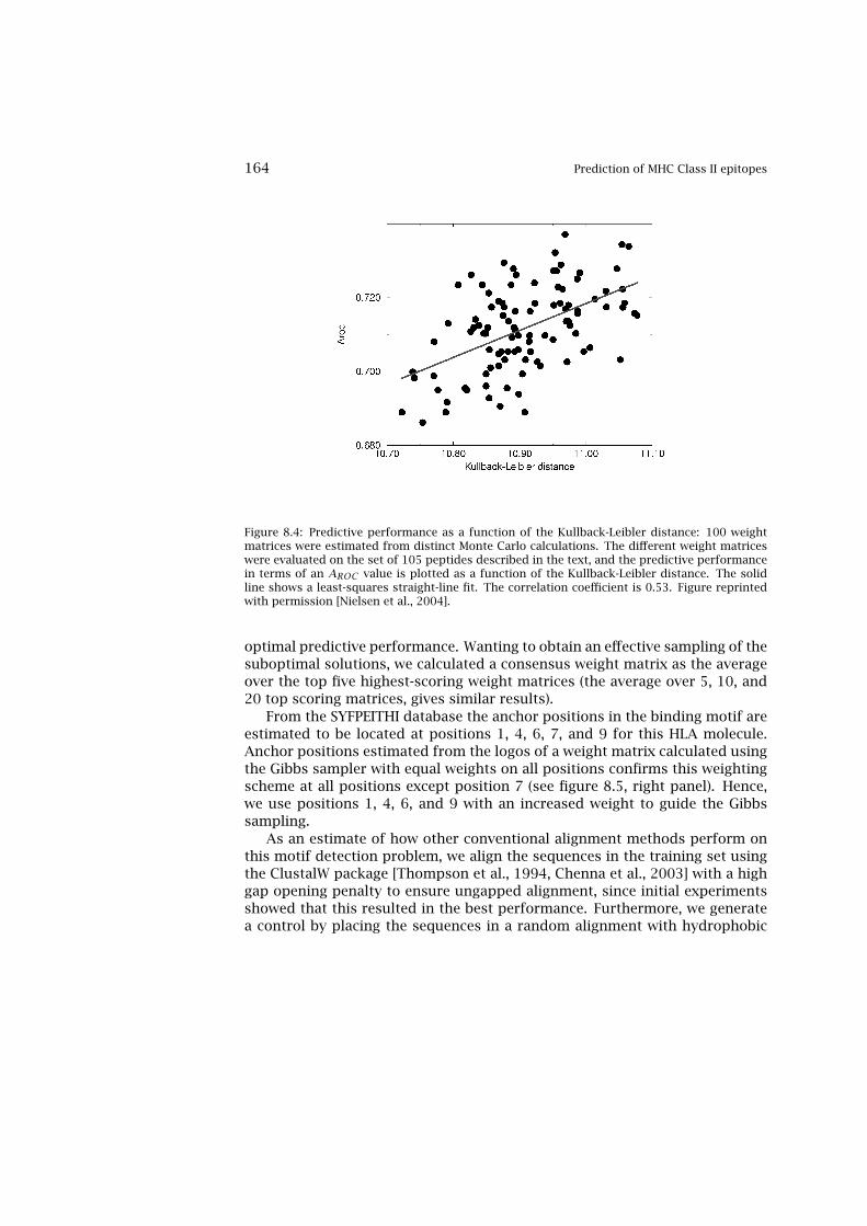
164 Prediction of MHC Class II epitopes
Figure 8.4: Predictive performance as a function of the Kullback-Leibler distance: 100 weightmatrices were estimated from distinct Monte Carlo calculations. The different weight matriceswere evaluated on the set of 105 peptides described in the text, and the predictive performancein terms of an AROC value is plotted as a function of the Kullback-Leibler distance. The solidline shows a least-squares straight-line fit. The correlation coefficient is 0.53. Figure reprintedwith permission [Nielsen et al., 2004].
optimal predictive performance. Wanting to obtain an effective sampling of thesuboptimal solutions, we calculated a consensus weight matrix as the averageover the top five highest-scoring weight matrices (the average over 5, 10, and20 top scoring matrices, gives similar results).
From the SYFPEITHI database the anchor positions in the binding motif areestimated to be located at positions 1, 4, 6, 7, and 9 for this HLA molecule.Anchor positions estimated from the logos of a weight matrix calculated usingthe Gibbs sampler with equal weights on all positions confirms this weightingscheme at all positions except position 7 (see figure 8.5, right panel). Hence,we use positions 1, 4, 6, and 9 with an increased weight to guide the Gibbssampling.
As an estimate of how other conventional alignment methods perform onthis motif detection problem, we align the sequences in the training set usingthe ClustalW package [Thompson et al., 1994, Chenna et al., 2003] with a highgap opening penalty to ensure ungapped alignment, since initial experimentsshowed that this resulted in the best performance. Furthermore, we generatea control by placing the sequences in a random alignment with hydrophobic

The Gibbs Sampler Method 165
ClustalW Random Gibbs
Figure 8.5: Logos of amino acid frequencies in three distinct alignments of the peptides inthe training set. The alignments are generated using ClustalW, a random placement, and theGibbs motif sampler, respectively. The height of a column in the logo is proportional to theinformation content in the sequence motif and the letter height is proportional to amino acidfrequency [Schneider and Stephens, 1990]. Figure reprinted with permission [Nielsen et al.,2004]. See plate 14 for color version.
amino acids at the p1 position. From the alignments, we estimate the aminoacid frequencies in the 9-amino acid long core region and make logos fromthese frequency estimates (shown in figure 8.5).
Figure 8.5 demonstrates that the identification of the binding motif fromthe training data is indeed a complex and difficult task. The ability of the Gibbssampler to detect the subtle sequence motif in a set of peptide sequences isapparent from the figure. ClustalW is, on the other hand, unable to detect anymotif except from the strong hydrophobic amino acid preference at positionp1. In figure 8.6, we show a part of the alignment obtained by the Gibbs sam-pler for the HLA-DR4(B1*0401) binding motif recognition. Figures 8.5 and 8.6demonstrate how the Gibbs sampler, through the Monte Carlo moves, is ableto place the sequences in register and move from an initial random configura-tion with close to zero information content to a final alignment configurationwith high information content describing the peptide binding motif in detail.
8.2.4 Benchmark Calculations
The predictive performance of the Gibbs sampler is benchmarked on 10data sets and compared to that of the TEPITOPE method [Sturniolo et al.,1999], as well as to the weight matrix derived from the ClustalW alignment.

166 Prediction of MHC Class II epitopes
Figure 8.6: An alignment generated by the Gibbs sampler for the DR4(B1*0401) binding motif. Inthe left panel are shown the unaligned sequences, and in the right panel the aligned sequences.The core motif is shown underlined and in italics. Figure reprinted with permission [Nielsenet al., 2004].
The 10 data sets are the eight data sets described by Raghava (MHCBench,http://www.imtech.res.in/raghava/mhcbench), and two experimental datasets described by Southwood et al. [1998] and Geluk et al. [1998], respectively.The binding of a peptide is calculated as the score of the highest-scoring 9mersubpeptide. We use the nonparametric AROC measure [Swets, 1988] to com-pare the accuracy of the different prediction methods. In order to calculate aROC curve the data set must be classified into binders and nonbinders. Forthe eight MHCBench data sets, peptides with an associated binding value ofzero are assigned to be nonbinding, and all other peptides are binders. For theSouthwood and Geluk data sets, an affinity of 1000 nM is taken as thresholdfor peptide binding [Southwood et al., 1998] (similar results are obtainedfor threshold values in the range 500–10,000 nM). To reduce the chance ofoverfitting by evaluating the prediction performance on data points includedin the training, we repeat the benchmark calculation on homology-reduceddata sets. The homology reduction is performed so that no data point in theevaluation sets has a match in the training set with sequence identity greaterthan 90% over an alignment length of at least 9 amino acids. Table 8.2 givesa brief description of both the original and the homology-reduced benchmarkdata sets in terms of the number of peptides and the number of binders,respectively.
In figure 8.7, we show the results of the benchmark calculation. The Gibbssampled weight matrix has comparable or better predictive performancethan that of both TEPITOPE and the ClustalW weight matrix. In all cases

The Gibbs Sampler Method 167
Original Homology-reducedSet N Nbind N NbindMHCBench 1 1017 694 496 226MHCBench 2 673 381 416 161MHCBench 3A 590 373 334 130MHCBench 3B 495 279 325 128MHCBench 4A 646 323 381 111MHCBench 4B 584 292 375 120MHCBench 5A 117 70 110 65MHCBench 5B 85 48 84 47Southwood 22 16 21 15Geluk 105 22 99 19
Table 8.2: Description of the MHC class II benchmark (MHCBench) data sets. The first columngives the name of the data set; the second and third columns, the number of peptides and thenumber of peptides classified as binders for the complete sets; the fourth and fifth columns,the same number for the reduced data sets. For the Southwood and Geluk data sets a thresholdof 1000 nM and for the MHCBench data sets a threshold value of 0.5, were used to determinebinders.
the ClustalW weight matrix has a performance that is lower than that of theGibbs sampled matrix. In order to estimate the significance of the differencein performance between the Gibbs sampler and the TEPITOPE methods, abootstrap experiment was performed [Press et al., 1992]. For each of thedata sets, 1000 data sets were generated by extracting N data points withreplacement. Here N is the number of data points in the original data set.The performances of both the Gibbs and the TEPITOPE methods are thenevaluated on each of the data sets, and the p-value for the hypothesis that theTEPITOPE method performs better than the Gibbs sampler is estimated as thefraction of experiments where TEPITOPE has the better performance of thetwo. The results of this calculation demonstrate that for five of the ten datasets (the Southwood set, set 1, set 2, set 4A, and set 4B) the Gibbs sampler hasa performance that is significantly higher than that of TEPITOPE (p < 0.05).Only for one data set (set 5B), does the TEPITOPE method perform better thanthe Gibbs sampler (p = 0.96). For the remaining four data sets the differencein predictive performance is found to be insignificant (0.05 < p < 0.95).
The average AROC values for the Gibbs sampler, the TEPITOPE matrix, andthe ClustalW matrix methods are 0.744, 0.702 and 0.667 for the complete dataset, and 0.673, 0.630, and 0.599 for the reduced data sets, respectively.
For two of the ten data sets (set 5A and set 5B) the TEPITOPE weight matrixhas a higher AROC value than the Gibbs matrix. For the set 5B this differenceis statistically significant (p = 0.96). In order to analyze why the Gibbs sam-pler has poor performance on the two data sets, we estimated the amino acid

168 Prediction of MHC Class II epitopes
Figure 8.7: Prediction accuracy for the Gibbs sampler, the TEPITOPE, and the ClustalW weight-matrix methods, for the ten benchmark data sets described in the text. For each data set thefirst three bars give the performance on the complete data sets, and the last three bars theperformance on the reduced data sets, respectively. Figure reprinted with permision [Nielsenet al., 2004].
composition in the two sets and compared it to that of the other benchmarksets and the training set. In this analysis, we find that both sets have an ex-tremely high content of cysteine in the subset of peptides that bind MHC. Inset 5B, e.g., 45 of the 85 peptides contain at least one cysteine, and 37 of the45 bind MHC. These numbers stand in contrast to the low cysteine content inthe training set. Here, only 47 of the 456 peptide sequences contain cysteine.The TEPITOPE weight matrix has a particular behavior for cysteines in that thescore for this amino acid at all positions is zero.
To verify whether the cysteine content could explain the poor behavior ofthe Gibbs sampler as compared to the TEPITOPE matrix method, we repeatedthe above benchmark calculation substituting all occurrences of cysteine withalanine in the benchmark data sets. The result of the calculation is shownin Figure 8.8. The Gibbs sampled weight matrix in the cysteine-substitutedbenchmark calculation also for the reduced data sets has a better or compara-ble predictive performance compared to that of the TEPITOPE matrix method.Especially, one should note that the performance on the two sets 5A and 5Bis comparable for the two methods. Repeating the bootstrap experiment for

The Gibbs Sampler Method 169
Figure 8.8: Cysteine-substituted benchmark. Prediction accuracy of the Gibbs sampled, theTEPITOPE, and the ClustalW weight-matrix methods for the ten benchmark data sets describedin the text. All occurrences of cysteine are replaced with alanine. For each data set the first threecolumns give the performance on the complete data sets, and the last three columns give theperformance on the reduced data sets. Figure reprinted with permission [Nielsen et al., 2004].
the set 5B, applying cysteine substitution, gave a p-value of 0.5. This demon-strates that it indeed was the unusual cysteine content that led to the poorperformance of the Gibbs sampler for the two data sets. Similarly, one shouldnote that the performance of the Gibbs sampler for the other eight data setsis similar to that shown in figure 8.5. The average AROC values for the Gibbssampled matrix, the TEPITOPE, and the ClustalW weight matrix, respectively,are 0.755, 0.703, and 0.692 for the complete data sets and 0.690, 0.630, and0.637 for the reduced data sets.
One other striking observation from figures 8.7 and 8.8 is the poor perfor-mance of the TEPITOPE method on the Southwood data set. A simple calcula-tion outlines a possible explanation for this poor performance. If one calcu-lates the odds (frequency/background) values for the amino acid compositionat the possible p1 positions in the Southwood data set, one finds that the threeamino acids with the highest odds ratios are F, W, and Y. This stands in con-trast to the finding in the other data sets where no particular bias is found inthe amino acids with the highest odds. The amino acid composition bias atthe p1 position in the Southwood data set originates from the selection bias in
170 Prediction of MHC Class II epitopes
the prediction algorithm used to select the peptides for binding assay verifica-tion [Southwood et al., 1998]). In the TEPITOPE weight matrix, the p1 positionis modeled in a very crude manner, in that all nonhydrophobic amino acidshave a value of -999, and the hydrophobic amino acids have a value of either0 (F, W, and Y) or 1 (I, L, M, and V). In the Gibbs sampler matrix, this pictureis more differentiated. Here the difference in weight matrix score between thecommon (I, L, M, and V) and the rare amino acids (F, W, and Y) is, on average,10. The importance of this distinction between the different allowed aminoacids becomes clear, if one sets the p1 weight matrix values for F, Y, and W ofthe TEPITOPE matrix to 9. Using the modified TEPITOPE matrix the AROC valueis increased to 0.80. The average performance on the other data sets in thebenchmark calculation is comparable to that of the original TEPITOPE matrix.
8.3 Further Improvements of the Approach
We have in this chapter shown how the Gibbs sampler method can be appliedfor detecting the binding motif for MHC class I and class II molecules. TheGibbs sampler method implements the techniques of sequence weighting andpseudocount correction for low counts. These techniques allow the algorithmto handle situations where only very few data points are available and limitthe effect of any sequence redundancy in the training data set.
Peptides binding to MHC class II are typically longer than the core motif andcorrect alignment is key to obtaining good prediction performance. The Gibbssampler performs well in this task. The optimal Gibbs sampler solution (theone with the highest information content) is not necessarily the optimal pre-dictor, and, as shown, including suboptimal solutions in an ensemble averageincreases the predictive performance of this method.
Prediction of class II MHC epitopes is a difficult task, and the predictionaccuracy of the described method is far from perfect. Moreover, as we demon-strated here, the nature of the test set can influence the performance resultsdrastically. At least two avenues exist where one can expect to achieve higheraccuracy. One avenue is the development of more sophisticated predictionmethods. For MHC class I a combination of many artificial neural networkswith different types of sequence encoding lead to predictors of improved ac-curacy [Nielsen et al., 2003]. Using the Gibbs sampler as an alignment prepro-cessing step as described by Brusic et al. [1998b], a similar approach mightbe beneficial for MHC class II predictions. A second avenue to improved pre-diction algorithms is the generation of relevant training data. For MHC classI the use of quantitative binding data as opposed to classification data leadsto higher accuracy predictors [Buus et al., 2003, Nielsen et al., 2003]. Further-more, a guided iterative training process where new data points are selected

Further Improvements of the Approach 171
from experimental binding assay verification by the methods like QBC (queryby committee) can, in a highly cost- and time-efficient manner, lead to high-accuracy prediction methods [Christensen et al., 2003]. A similar approachmight be applied to the MHC class II problem. The weight matrix obtainedby the Gibbs sampler or other methods can generate first-generation peptidepredictions for verification in binding affinity assays. Subsequently, the QBCmethod can guide the process of generating informative data that upon exper-imental verification can in turn provide high quality-prediction methods.


Chapter 9
Processing of MHC Class IIEpitopes
The degradation of the antigen in the MHC class II pathway is rather differentfrom that in the MHC class I pathway (see figure 9.1). First of all, in the MHCclass II pathway mainly the exogenous proteins are presented. Protein intakethrough endocytosis leads to formation of endosomes, which become increas-ingly acidic as they progress and eventually fuse with lysosomes. These vesi-cles contain aspartic and cysteine proteases, which are activated as the acidityincreases and thereby degrade the protein into peptides (for a recent review,see Watts [2004]). The protease activity can generate and destroy MHC class IIepitopes. The peptides susceptible to destructive processing might survive ifthey can be loaded to MHC class II molecules early. The MHC class II moleculesthemselves are quite resistant to proteolysis; therefore the core peptide is com-pletely protected while the rest of the peptide can be trimmed by endosomalendopeptidases hydrolyzing internal amide bonds and exoproteases hydrolyz-ing one or two amino acids from either the N- or C-terminal [Chapman, 1998].A type II membrane protein, called the invariant chain (Ii), is associated withnewly synthesized MHC class II proteins in the ER. Ii stabilizes MHC moleculesand directs transportation to early endosomes. Proteolytic cleavage of Ii is im-portant for the correct peptide loading of MHC class II. A part of Ii, called CLIP(class II associated invariant chain), occupies the peptide binding groove ofthe MHC class II molecule. Interaction of MHC class II with a MHC class II-likemolecule (called HLA-DM in humans), catalyzes the release of CLIP allowingother peptides to bind [Watts, 2004]. In this chapter, we review the specificityof the many proteases playing a role in MHC class II antigen processing andreport some results on analyzing the specificity of these enzymes.
173

174 Processing of MHC class II epitopes
Figure 9.1: The MHC class II presentation pathway. Newly synthesized MHC molecules are sta-bilized by Invariant chain (Ii) in ER and transported to exocytic vesicles via the trans-Golgi net-work. Alternatively, the MHC-Ii complex can be transported to the membrane and then rapidlyinternalized into endosomes. Mature endosomes/lysosomal containing degradation productsof proteins fuse with exocytic vesicles. Due to high enzymatic activity in the fused vesicles Iiis degraded, however, the binding groove of MHC molecule remains occupied by CLIP. HLA-DM(an MHC class II-like molecule, not shown in the figure) regulates the removal of CLIP and allowspeptide binding. The MHC-peptide complex is then transported to the cell membrane. Figurecourtesy of Maite Severins.
9.1 Enzymes Involved in Generating MHC Class II Ligands
Processing of antigens in the MHC class II pathway is achieved by many differ-ent peptidases [Watts, 2004]. The principal enzymes and their specificity arebriefly reviewed here; for a more extensive review, see Honey and Rudensky[2003]. Each enzyme can be quite specific and often these specificities do notoverlap. A key question is the level of redundancy in the system: how large apart of these specificities are indeed necessary to be able to develop sufficienthelper T cell responses? Is each enzyme responsible on its own for generatinga specific response, or is “generic” protease activity sufficient? Also, we wouldlike to know how the hierarchy of the epitopes (immunodominant, dominant,subdominant) is affected by the specificity and distribution of these enzymes.

Enzymes Involved in Generating MHC Class II Ligands 175
Name Protease Family Expression PreferenceCathepsin L C1 B cells, Dendritic cells (DCs), ?
thymocytesCathepsin S C1 B cells, DCs, macrophages, ?
epithelial cellsCathepsin B C1 B cells, DCs, macrophages –Arg-Arg-|-XaaCathepsin C C1 Mast cells, B cells Xaa-Xbb-|-Xcca
Cathepsin D A1 B cells, DCs, macrophages –Ala-Phe-|-Phe-AlaCathepsin E A1 B cells Arg-Arg bondsCathepsin F C1 Epithelial cells, macrophages ?Cathepsin K C1 Osteoclasts, macrophages ?Cathepsin H C1 Monocytes, spermatids ?
a Except when Xaa is Arg or Lys, or when Xbb or Xcc is Pro.
Table 9.1: Major cathepsins involved in antigen processing in lysosomes. The protease family Ccontains cysteine proteases, while A is aspartic proteases.
At the moment, we have little data available to be able to answer these ques-tions. More information about peptidases is available in the MEROPS database(merops.sanger.ac.uk, [Rawlings et al., 2004]).
9.1.1 Cathepsins
Most mammalian lysosomal cysteine proteases are cathepsins. Cathepsinshave been identified as key regulatory enzymes for MHC class II presenta-tion, because they degrade Ii, as well as the antigen [Honey and Rudensky,2003, Watts, 2004, Ebert et al., 2002]. Table 9.1 gives a summary of differenttypes of cathepsins involved in antigen presentation. Cathepsins, like pro-teases in general, are divided into four groups according to the identity of thecritical residue in their active site. Cysteine-, aspartyl-, serine-, and metallo-proteases (cathepsins) have cysteine, aspartate, serine, and metal ions in theiractive sites, respectively, which serve as nucleophiles during the attack on thecarbonyl carbon of the amide bond.
Recent studies have pointed to novel roles for cathepsins. For example,cathepsins C and S regulate the levels of stored proteases in the mast cellsecretory granules [Henningsson et al., 2003] and cathepsin L plays a role incell signaling [Chapman, 2004]. In B lymphoblastoid cells cathepsin B is foundin early and late endosomes, but absent from lysosomes, while cathepsins H,S, D, and C are distributed between late endosomes and lysosomes [Lautweinet al., 2004]. This suggests that cathepsin B might be involved in the initialproteolytic attack on a given antigen.
Little is known about how cathepsins, together with other lysosomal pro-

176 Processing of MHC class II epitopes
teases, work in vivo to generate T cell epitopes. However, in vitro analysiswith purified cathepsins has recently identified the specificity of some cathep-sins. Cezari et al. [2002] found that cathepsin B, a thiol protease, has a broadspecificity for peptide bonds, but preferentially cleaves –Arg-Arg-|-Xaa (Xaaany amino acid) bonds in small molecules. Cathepsin C has similar broadspecificity, but preferentially cleaves Xaa-Xbb-|-Xcc, except when Xaa is Arg orLys, or when Xbb or Xcc is Pro [Turk et al., 2001]. Cathepsin H can act as anaminopeptidase as well as an endopeptidase, and has a preference for cleav-ing after Arg [Dodt and Reichwein, 2003]. Both aspartic proteases, cathepsinD and E, also play a role in intracellular protein degradation, in addition tothe generation of antigenic peptides. Cathepsin D has a preference for cleav-ing after hydrophobic residues, especially –Ala-Phe-|-Phe-Ala [Pimenta et al.,2001]. Cathepsin E was found to have a special preference for Arg-Arg bonds;however, this is only confirmed in neutral pH and it remains doubtful whetheror not this preference would be the same in the acidic lysosome environment[Athauda and Takahashi, 2002].
9.1.2 Interferon–Gamma Reducible Lysosomal Thiol Protease (GILT)
In humans, GILT is constitutively present in late endocytic compartmentsof antigen presenting cells (APCs). GILT belongs to the thioredoxin family,and catalyzes the reduction of disulfide (S-S) bonds in protein substrates[Arunachalam et al., 2000]. To assess the involvement of GILT in MHC classII-restricted presentation of antigenic proteins containing disulfide bonds,Maric et al. [2001] generated a GILT-deficient mouse. In the absence of GILT,presentation of two major lysozyme antigenic epitopes to T cells is partiallyor completely abrogated. These data provide the first demonstration that thepool of proteolytic enzymes found in the endocytic pathway is not alwayssufficient to release the full spectrum of peptides for T cells to respond. GILTis likely to have an impact on the array of peptides (especially from proteinscontaining disulfide bonds, like hen egg lysozyme) constitutively presentedon APCs in lymphoid organs.
9.1.3 Alanyl Aminopeptidase N (APN)
APN (or CD13) is a transmembrane ectoenzyme occurring on a wide varietyof cells. In contrast to monocytes and granulocytes, lymphocytes of periph-eral blood do not express APN. APN can trim the N-terminal of any peptide,although it slows down whenever it encounters a proline [Dong et al., 2000].Almost all of the lysosomal proteases are not able to further degrade the pep-tides once they are bound to MHC class II molecules. However, Larsen et al.
Selective Loading of Peptides to MHC Class II Molecules 177
[1996] showed that the N-terminal of the peptide could, even while bound toMHC class II molecules, be digested by APN. This can directly effect T cellantigen recognition.
9.1.4 Asparaginyl Endopeptidase (AEP)
AEP is solely responsible for processing of microbial tetanus toxin antigen[Manoury et al., 1998]. AEP seems to be a very specific enzyme: it uses onlyasparagine as a cleavage site; however 10% of all asparagines in a protein areindeed cleaved [Dando et al., 1999]. AEP might be a very important enzyme inthe MHC class II pathway, because some data suggest that other lysosomal pro-teases can degrade some proteins, e.g., mylein basic protein, only if the initialcleavages are made by AEP [Beck et al., 2001]. Thus, AEP on its own can de-termine the antigenicity of some proteins. Deficiency in AEP is not lethal: AEPknockout mice were normally born and fertile, although their body weightswere significantly reduced [Shirahama-Noda et al., 2003]. The processing oflysosomal proteases (cathepsins B, H, and L) into efficient forms depends fullyon AEP, making AEP again a crucial player in the generation of MHC class IIepitopes. Plant homologs of mammalian AEP seem to have a similar function,i.e., they degrade proenzymes in storage vesicles.
9.2 Selective Loading of Peptides to MHC Class II Molecules
Since new MHC class II molecules reach endosomal/lysosomal compartmentswhile bound to Ii, epitope presentation is totally dependent on the degradationof Ii. Only after this degradation will the binding groove be able to bind otherpeptides. Ii degradation occurs in a stepwise manner. The initialization of Iidegradation is done by AEP [Manoury et al., 2003], but might be performedby other proteases as well. The subsequent steps involve cathepsins S and L[Honey and Rudensky, 2003]. Deficiency in cathepsin S or L can reduce thehelper T cell repertoire to 30% (first shown by Nakagawa et al. [1998]). Thiseffect is not only due to impairment of the Ii degradation [Honey et al., 2002],but also because of inefficient positive selection, as the MHC class II boundpeptide ligand repertoire is severely reduced. After degradation, part of Ii,CLIP, remains bound to the MHC molecule.
Removal of CLIP and peptide loading of MHC class II molecules require yetanother accessory molecule, designated HLA-DM in human and H2-M in mouse(for a review see [Kropshofer et al., 1999, Brocke et al., 2002]). HLA-DM is anMHC class II-like molecule which is nonpolymorphic. The binding of HLA-DMto the HLA-DR (one of the three HLA class II loci) molecule enables an openconformational state of the peptide binding groove [Kropshofer et al., 1996].
178 Processing of MHC class II epitopes
This open state probably allows for the release of CLIP and leaves the complexof the HLA-DM and MHC class II molecule available for binding other peptides.Only stably binding peptides can bring the groove back to the closed state andstabilize the HLA-DR molecule. In this case HLA-DM dissociates, allowing theHLA-DR-peptide complex to travel to the cell surface and interact with helper Tcells. A low-affinity peptide would not be able to achieve dissociation of HLA-DM molecules, and thus may be easily exchanged for a higher-affinity peptide.This reaction follows the rules of Michaelis-Menten kinetics, where HLA-DMacts like a catalyst. Because of this peptide editing property, HLA-DM is animportant player in the antigen presentation pathway. The peptide editing caneven continue on the cell surface: about 10 % of HLA-DM can be found on thesurface of the B cells and dendritic cells [Arndt et al., 2000]. HLA-DM deficientcells cannot perform antigen presentation on MHC class II molecules, becauseCLIP remains bound to the peptide binding groove.
In the MHC class I pathway, tapasin has a similar role in facilitating peptideloading and selecting the optimal ligands (for a review, see, e.g., [Brocke et al.,2002]). Tapasin and HLA-DM are structurally different and their sole func-tion seems to be the regulation of peptide loading of MHC molecules. Thesetwo molecules apparently allow for keeping otherwise instable MHC molecules“in waiting”, which might be essential for rapid presentation of peptides frompathogens in infected cells. Several autoepitopes causing autoimmune dis-eases have been reported to be low-affinity binders of disease-associated MHCclass II molecules. It is possible that the real cause of autoimmunity in thosecases are mistakes in regulation of tapasin and HLA-DM at the gene and pro-tein level.
As in the MHC class I presentation pathway, the pathogens try to evadeCD4+ T cell responses via blocking presentation on the MHC class II molecules.To our knowledge there are no examples of specific evasion from degradationin lysosomes/endosomes. However, several viruses can downregulate MHCclass II expression, degrade HLA-DM molecules, or interfere with the transportof MHC class II complexes (for a review, see Vossen et al. [2002]).
9.3 Phylogenetic Analysis of the Lysosomal Proteases
Classification schemes based on the overall structure of the proteins [Barrettand Rawlings, 2001] assign cathepsins to two families of lysosomal proteases,the S1 family (represented by the serine protease cathepsin G) and the C1 fam-ily. Within the C1 family, the aspartyl proteases (cathepsins D and E, alsocalled the A1 subfamily) are thought to have diverged from the cysteine pro-teases. This division is also clear in the phylogenetic analysis based on humansequences given in figure 9.2. The analysis comprises thirteen cathepsin se-

Phylogenetic Analysis of the Lysosomal Proteases 179
Figure 9.2: Phylogenetic tree of the enzymes involved in generating MHC class II epitopes. Thir-teen cathepsin sequences, as well as GILT, AEP, and APN, are included.
quences, and the GILT, AEP, and APN sequences. All the cathepsins exceptCATG, CATD, and CATE are cysteine proteases. CATE and CATD are aspartylproteases, and CATG is a serine protease. GILT, AEP, and APN are the pro-teases described in sections 9.1.2–9.1.4. The cathepsins are placed in threegroups: All cysteine proteases form one group, the aspartyl proteases (CATEand CATD) another group, and CATG, GILT, AEP, and APN form isolated groupswith branches connected close to the root of the tree, showing that these se-quences share no or only have very remote sequence homology.
Although several proteases mentioned in this chapter have been identifiedin a variety of organisms, little is known about the phylogenetic relationshipbetween these enzymes involved in antigen processing. Using cephalochor-date, agnathan, and bony fish cathepsins, together with cathepsin sequences

180 Processing of MHC class II epitopes
available from other vertebrates, Uinuk-Ool et al. [2003] studied the evolutionof the cathepsin family. They found that all cathepsins originate from two veryold lineages, the B and the L lineages, which diverged early in the evolution ofeukaryotes.
The emergence of the adaptive immune systems seems to have increaseddramatically the size of the cathepsin family. Presumably, at first, the phyloge-netically oldest cathepsins with broad tissue distribution are used to generatethe peptide pool for MHC class II molecules, like cathepsin B and L. Later, sev-eral gene duplications resulted in more tissue-specific cathepsins, like cathep-sin S, which is found mainly in APCs and thymocytes [Driessen et al., 1999].Since these enzymes have different specificities, the differentiation in the tis-sue distribution seems to be an efficient way of presenting different sets ofpeptides on different cell types.
9.4 Signs of the Specificities of Lysosomal Proteases on MHCClass II Epitopes
The MHC class II compartment hosts several (most yet unknown) regulationsystems that balance the creative and destructive proteolytic forces on antigensubstrates. The final peptide presented on MHC class II molecules is a resultof the combination of all enzymatic specificities summarized above. A logo ofa large set of epitopes found the SYFPEITHI database [Rammensee et al., 1999]known to bind HLA class II (706 epitopes from 62 HLA types) demonstratesthis (see figure 9.3). In the figure is shown a logo of the N-terminals (leftpanel) and C-terminals (right panel) of peptides presented by MHC class II.The flanking regions of the epitopes were identified by locating the protein“hosting” the epitope in the Swiss-Prot database [Bairoch and Apweiler, 2000].
Clearly, at the N-terminals the signal is stronger than at C-terminals. Prob-ably the abundance of Pro at position 2 of the epitope shows signs of thecleavage-inhibiting motif of, e.g., ANP. At the C-terminals all enzymes can beacting, reducing the signal/motif to a minimum.
9.5 Predicting the Specificity of Lysosomal Enzymes
Reliable prediction tools on peptidase/protease specificity are not available,because data on substrate specificity of lysosomal enzymes are very limited.One promising approach is 2D gel electrophoresis, in conjunction with tan-dem mass spectrometry (MS), which can potentially identify and characterizenatural enzyme substrates and their products. Bredemeyer et al. [2004] chosethe serine protease granzyme (Gzm) B as a test enzyme to evaluate this ap-
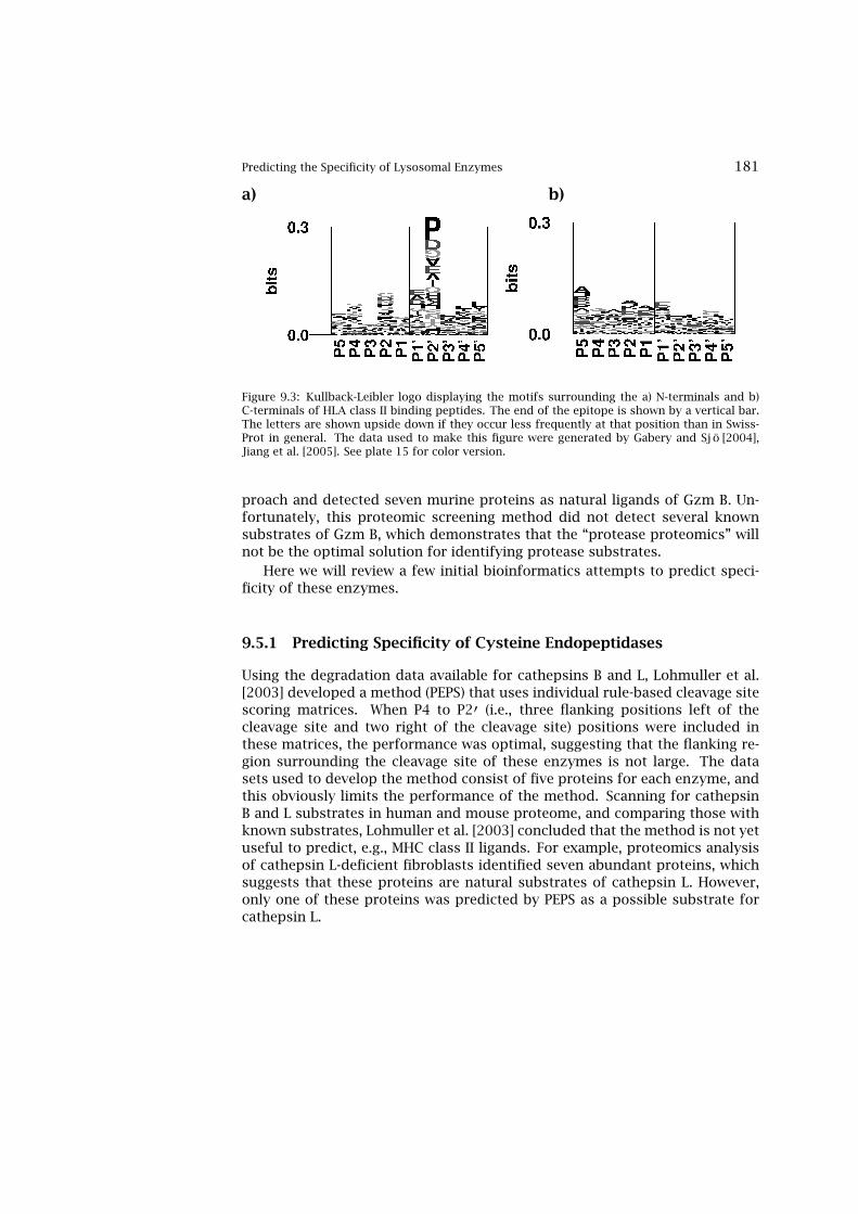
Predicting the Specificity of Lysosomal Enzymes 181
a) b)
Figure 9.3: Kullback-Leibler logo displaying the motifs surrounding the a) N-terminals and b)C-terminals of HLA class II binding peptides. The end of the epitope is shown by a vertical bar.The letters are shown upside down if they occur less frequently at that position than in Swiss-Prot in general. The data used to make this figure were generated by Gabery and Sjö [2004],Jiang et al. [2005]. See plate 15 for color version.
proach and detected seven murine proteins as natural ligands of Gzm B. Un-fortunately, this proteomic screening method did not detect several knownsubstrates of Gzm B, which demonstrates that the “protease proteomics” willnot be the optimal solution for identifying protease substrates.
Here we will review a few initial bioinformatics attempts to predict speci-ficity of these enzymes.
9.5.1 Predicting Specificity of Cysteine Endopeptidases
Using the degradation data available for cathepsins B and L, Lohmuller et al.[2003] developed a method (PEPS) that uses individual rule-based cleavage sitescoring matrices. When P4 to P2′ (i.e., three flanking positions left of thecleavage site and two right of the cleavage site) positions were included inthese matrices, the performance was optimal, suggesting that the flanking re-gion surrounding the cleavage site of these enzymes is not large. The datasets used to develop the method consist of five proteins for each enzyme, andthis obviously limits the performance of the method. Scanning for cathepsinB and L substrates in human and mouse proteome, and comparing those withknown substrates, Lohmuller et al. [2003] concluded that the method is not yetuseful to predict, e.g., MHC class II ligands. For example, proteomics analysisof cathepsin L-deficient fibroblasts identified seven abundant proteins, whichsuggests that these proteins are natural substrates of cathepsin L. However,only one of these proteins was predicted by PEPS as a possible substrate forcathepsin L.

182 Processing of MHC class II epitopes
AEP cleavage sites Non preferred sites
Figure 9.4: The sequence logo of AEP cleavage sites with their flanking region (left panel) and asimilar logo for all the other asparagine residues in the proteins studied (right panel). Part of thedata was kindly provided by Dr. Colin Watts, University of Dundee, and the rest was extractedduring a literature study. See plate 16 for color version.
9.5.2 Predicting Specificity of AEP
At the moment AEP cleavage sites are known in 18 proteins [Manoury et al.,1998, Dando et al., 1999, Beck et al., 2001, Mathieu et al., 2002, Antoniou andWatts, 2002, Sarandeses et al., 2003]. These proteins have 402 asparagineresidues, where only 42 are used by AEP as a cleavage site. Three proteins,horse myoglobin, rat tyrosine aminotransferase, and horse ferritin, are resis-tant to AEP, which gives a total of 27 asparagine residues that are definitelynot used by AEP as cleavage sites. A sequence logo of the sites that are cleavedby AEP and the flanking regions of other asparagines (i.e., the ones that are notcleaved) are shown in figure 9.4.
Since AEP can cleave folded proteins efficiently, it was first studied whetheror not the cleavage sites that are used by AEP occur on the surface of theproteins. Of 42 cleavage sites, 25 occur in “exposed” regions; however, also50% of the asparagines that are resistant to AEP cleavage occur in the exposedregions. Thus, being exposed does not seem to be a discriminatory factorfor AEP cleavage prediction. There can be two explanations for this. First,this result is based on surface accessibility predictions, which are only 75%accurate. Second, the lysosomes are highly acidic environments, which cancause the unfolding of the protein before coming into contact with AEP.
Another biological process that seems to play a role in AEP cleavageis N-glycosylation. Manoury et al. [1998] report that N-glycosylation can
Predicting the Specificity of Lysosomal Enzymes 183
eliminate sites of processing by AEP. There are two main motifs defined for N-glycosylation: the Asn-Xaa-Thr and Asn-Xaa-Ser motifs (Where Xaa is not Pro).The Asn-Xaa-Thr motif was never found among the cleavage sites in this dataset. Asn-Xaa-Ser occurs twice, but in both cases N-glycosylation is not pre-dicted according to the NetNGlyc server (www.cbs.dtu.dk/services/NetNGlyc).So N-glycosylation can be used as a filter to predict AEP cleavage sites.
A series of neural networks are trained to predict AEP specificity based onthe known AEP cleavages and proteins resistant to AEP cleavage (C. Kesmir& C. Watts, unpublished results). Neural networks have earlier been used topredict the specificity of viral proteinases of SARS and picornaviruses [Blomet al., 1996, Kiemer et al., 2004]. All positions between P4 and P3′ are necessaryto get better predictions. The effect of neighboring residues on AEP cleavagemight depend on each other (e.g., the effect of Ala in P3 is determined alsoby which amino acid is found at P2′), because a neural network without anyhidden neurons, i.e., a linear prediction method, performs very poorly. Thissuggests that a nonlinear prediction method might be necessary to predict AEPspecificity, although having more data might prove that this statement is notvalid. Preliminary results suggest that it is possible to develop a method whichis able to predict 72% of the AEP cleavage sites, while identifying 90% of thenoncleavage sites (i.e., the asparagines that are not used by AEP) correctly (C.Kesmir & C. Watts, unpublished results). This results in a Matthews correlationcoefficient of 0.60. If more data become available, the performance of such apredictor will most likely increase.


Chapter 10
B Cell Epitopes
The humoral response is mediated by antibodies (immunoglobulin molecules),which are produced by B lymphocytes. B lymphocytes can bind to antigens bytheir immunoglobulin receptors. When they become activated, they start to se-crete a soluble form of this receptor (antibodies) in large amounts; figure 10.1shows an example of an antibody molecule. Note the overall Y-shape (or T-shape) of the antibody with the two antigen binding (Fab) fragments shown atthe top left and right of the antibody and the constant fragment (Fc) shown
below. The linker regions connecting the constant with the variable regionsallow great flexibility in the relative orientation of the domains. The highlyvariable tip of a Fab fragment that can bind to epitopes is called the paratopeand is made up of the so-called complementary determining regions (CDRs) inthe antibody sequence.
The binding of antibodies to, e.g., a virus, can coat the surface so that it can-not infect cells [Burton et al., 2001]. Viruses or bacteria covered by antibodiesare also more easily taken up (phagocytosed) and destroyed by scavenger cellsof the immune system such as macrophages. These cells can take up the anti-gen using their receptors for the constant Fc part of the antibody molecules.Antigens covered by antibodies can also activate the complement system. Thiscan lead to lysis of bacteria and enveloped viruses by the creation of a pore(membrane attack complex) in the membrane. Complement components onthe surface of microorganisms can also facilitate phagocytosis, by immunecells with complement receptors.
Contrary to T cells that recognize fragments of proteins bound to MHCmolecules, the antibodies recognize a protein in its native form without itbeing cleaved or bound to molecules such as the MHC molecules. This en-ables immune responses to extracellular pathogens. Therefore, the antibodyresponse is crucial in the defense against most pathogens. The fact that B
185

186 B cell epitopes
A B
Figure 10.1: Schematic cartoon (A) and surface (B) representation of an intact antibody (PDBentry 1IGT [Harris et al., 1997]). The light chains are shown in orange, the heavy chains inblue and green. The graphical representations of molecules in this chapter were prepared usingPYMOL (www.pymol.org, [Liang et al., 2003]). Figure courtesy of Thomas Blicher. See plate 17for color version.
cells recognize the folded structure of the antigen makes prediction of B cellepitopes much more difficult than the prediction of T cell epitopes.
In this chapter, we will review germinal center (GC) reactions where the an-tibody responses go through several rounds of mutation and selection, and wewill shortly discuss the mathematical models that are developed to addressoptimal mutation schema, selection mechanisms, and kinetics of the affinitymaturation. Having understood how effective antibody responses are gener-ated, we will then explain the principles behind B cell epitope prediction.
10.1 Affinity Maturation
Early in the primary immune response, the antibodies are of poor quality, i.e.,of low affinity. In order to provide long-lasting immunity, antibodies must ac-quire much higher affinity and should remain in the body in high amounts.This is achieved by a process called “affinity maturation.” There are two com-ponents which are essential for affinity maturation to take place. First, B cellsmust generate a high frequency of mutations (hypermutation) to produce largenumbers of mutants with different affinities. Second, there has to be a strongmechanism of selection of mutants that encode high-affinity antibodies. GCsare specialized microenvironments in secondary follicles that provide the rightconditions for affinity maturation to take place [Berek et al., 1991, MacLen-nan, 1994, Jacob et al., 1991, Leanderson et al., 1992] (see figure 10.2 for an

Affinity Maturation 187
Memory
Plasma cell
C*
C
C
Follicular Dendritic
Cell
Antigen
Apoptosis
Dark Zone
Light Zone
T
Figure 10.2: Overview of the germinal center reaction. Antigen specific B cells shortly afterentering germinal centers down-regulate their B cell receptor (BCR) and undergo rapid cell pro-liferation in the dark zone (dotted circles). During these cell divisions BCR genes accumulatesomatic mutations. After a number of cell divisions, the affinity of the cell is evaluated. The cellchanges its phenotype, re-expresses the BCR (circles marked with ‘C’), and competes with otherB cells to bind the antigen (filled small circles) on follicular dendritic cells (FDCs). If antigenbinding is successful, the B cell gets enough survival signal to go and search for a T cell (circlesmarked with ‘T’). The cognate interaction with T cell might ensure selecting only the B cells thatare after somatic mutations still unreactive to self [van Eijk et al., 2001]. Failure during antigenbinding or interaction with T cell results in apoptosis. The successful cells can (1) differentiateto plasma or memory B cells and leave the germinal center reaction, or (2) recycle back to thedark zone and repeat the proliferation-selection cycle. Adapted from Kesmir and de Boer [1999].
overview of GC reactions).
10.1.1 How are High Affinity Antibodies Generated?
In a GC environment activated B cells switch on a hypermutation mechanismthat affects the variable region of the B cell receptor and alters the affinity ofthe antibodies they encode [Betz et al., 1993, Yelamos et al., 1995, Wiens et al.,1998, Klein et al., 1998, Kelsoe, 1999, Wabl et al., 1999]. The mutation rateis roughly 10−3 per base pair per division [Berek and Milstein, 1987], whichis six orders of magnitude higher than spontaneous mutations. Mutations arenot evenly distributed throughout the variable region of the B cell receptor,but are concentrated in CDRs, which encode the amino acids that make con-
188 B cell epitopes
tact with the antigen [Levy et al., 1988]. Transitions are more frequent thantransversions, and both strands are hypermutation targets (for a review, see[Jacobs and Bross, 2001]). Analysis of large databases of somatically mutatedantibodies reveals that {A,G}G{C,T}{A,T} seems to be a common target for thehypermutation machinery. Especially, AGC and AGT triplets (both coding forserine) are mutating more than other codons [Levy et al., 1988]. The proteinnecessary for switching on hypermutation in B cells is the activation-inducedcytidine deaminase [Muramatsu et al., 2000], although this protein does notseem to be necessary to initiate GC reactions.
With such a high mutation rate, each B cell is expected to produce ap-proximately one mutant per cell division. Somatic mutations are generally ofno benefit: in most of the cases they lead to loss of antigen binding. Onepuzzling feature of affinity maturation is the efficiency by which high-affinitymutants are achieved. Kepler and Perelson [1993b] approached this questionfrom an optimal control perspective and calculated the schema of the hyper-mutations that would most efficiently generate high-affinity mutants. It is im-portant that a higher-affinity B cell mutant does not mutate again to becomea low-affinity mutant. They suggested that if a GC reaction consists of cyclesof mutation-free proliferation, followed by mutation and selection, one couldovercome the mutational decay of high-affinity mutants. These cycles couldoccur if the selected mutants instead of leaving GC traverse back to the pro-liferation area. The model of Kepler and Perelson [1993b] was received withgreat interest in the immunology community, and to date it has probably beenthe mathematical model that initiated most experimental studies to prove itsconclusions. However, more than a decade of research has not managed toprove that the suggested schema of the hypermutation is the correct in vivoscenario.
10.1.2 Competition Among B cells
The antigen is stored in the form of immune complexes on follicular dendriticcells (FDCs). Each new B cell mutant must bind to an antigen in order to avoidapoptosis [Koopman et al., 1997]. This basic fact makes the antigen the mainselective agent of a GC reaction. The strong selection in GCs results in anall-or-none behavior: GCs either contain hardly any high-affinity cells, or theyare almost completely taken over by high-affinity mutants [Radmacher et al.,1998, Berek et al., 1991]. This all-or-none behavior implies that take-over ratesare extremely high; Radmacher et al. [1998] calculated the take over rate of amutant, having a ten-fold increase in affinity, to be four per day. In the lastdecade many theoretical models of affinity maturation have been published(e.g., [Kepler and Perelson, 1993a,b, Oprea and Perelson, 1997, Oprea et al.,

Recognition of Antigen by B cells 189
2000]). These models, although good at simulating the average behavior ofa GC, are poor in explaining the all-or-none behavior. The major reason forthis pitfall is the use of affinity-proportional selection mechanisms, where Bcells compete with each other indirectly for available antigen. In addition, theselection decreases when the affinities of the competing cells increase.
To obtain better insights into the selection mechanisms, a spatial GC modelhas been developed in which B cells move, die, divide, and mutate. The for-malism used was first developed for adhesion-based sorting by Graner andGlazier [1992] and Glazier and Graner [1993], and was extended to representa GC reaction by Kesmir and de Boer [2003]. In this model, B cells competewith each other for getting enough space (i.e., for getting enough survival sig-nals) on the FDC surface. A spatial affinity-based sorting of the B cells on theFDC can be obtained if it is assumed that B cells with increased affinity havean increased cellular adhesion to the FDC presenting antigen. This leads toa “winner-takes-all” selection because, by the adhesion-based cellular sorting,only the highest-affinity B cells receive survival signals and are rescued by FDC[Kesmir and de Boer, 2003].
10.1.3 Role of T Cells in GC Reactions
To initiate a GC reaction, B cells should present antigen effectively to activatedT cells surrounding the follicle; the importance of this cognate interaction isshown in Garside et al. [1998]. The initial dependence of a GC reaction on T cellhelp seems to continue after GCs are established. Following affinity-based se-lection, GC B cells have to perform efficient cognate interactions with T cells toincrease their survival chance [MacLennan et al., 1997a, Lindhout et al., 1997].Interference with the cognate interaction between GC T and B cells disturbsthe GC reaction [Linsley et al., 1992, Ronchese et al., 1994, Gray et al., 1994,Han et al., 1995, MacLennan et al., 1997b].
The role of T cells in GC reactions has been studied in a mathematicalmodel [Kesmir and de Boer, 1999]. The model suggests that T cells play amajor role at the onset of the GC reaction; later only very few T cells sufficeto keep a GC reaction going. This is because at later stages of the GC reactionfluctuations in the number of rescued B cells are compensated by their highproliferation capacity.
10.2 Recognition of Antigen by B cells
Having an understanding of how high-affinity B cells are generated during animmune response, we will now switch to the antigenic regions recognized byB cells. B cell epitopes are normally classified into two groups: continuous

190 B cell epitopes
and discontinuous epitopes. A continuous epitope, (also called a sequential orlinear epitope) is a short peptide fragment in a protein that is recognized byantibodies specific for that protein. A discontinuous epitope is composed ofresidues that are not adjacent in the primary structure (amino acid sequence),but are brought into proximity by the folding of the polypeptide chain (seefigure 10.3 for an example). The classification is not clear-cut as discontinuousepitopes may contain linear stretches of amino acids, and continuous epitopesmay show conformational preferences. This is illustrated in figure 10.4, whichshows an example of an antibody interacting with a birch pollen protein (anallergen). Even though the central binding site is a loop protruding from thesurface, the antibody also interacts with amino acids from other parts of theamino acid chain of the allergen.
The typical protein-antibody complex has the following properties [van Re-genmortel, 1996]:
• Contact area of 700-900 Å.
• Amino acids from most CDR regions participate in binding; half of theseare aromatic amino acids.
• Discontinuous epitopes are formed by two to five participating regions.
• Binding affinity Ka is typically in the range of 10−7 - 10−9M.
• Up to 48 water molecules may be present in the binding interface.
• Binding is enthalpy-driven, not entropy-driven.
• Mutations outside the contact area may influence binding affinity.
Ninety percent of antibodies raised against a protein react with discontinu-ous fragments (reviewed by van Regenmortel [1996]). This makes B cell epitopeprediction a very challenging research field. Predicting continuous epitopes isa simpler problem, and to identify continuous epitopes may be still useful forsynthetic vaccines or as diagnostic tools [van Regenmortel and Muller, 1999].Predicted continuous epitopes may be used to immunize animals to produceantibodies that are cross-reactive with the native protein [van Regenmortel andPellequer, 1994]. Moreover, continuous epitope predictors can be integratedin prediction of discontinuous epitopes, as the latter epitopes often containlinear stretches [Hopp, 1994].
10.2.1 Prediction of Continuous Epitopes
The first method for predicting antigenic determinants (linear B cell epitopes)was developed by Hopp and Woods [1981, 1983]. The basic assumption of

Recognition of Antigen by B cells 191
Figure 10.3: An example of binding between a discontinuous epitope and the CDR regions of aspecific antibody: the factor VII protein and a Fab fragment from an inhibitory antibody (PDBcode 1IQD Spiegel et al. [2001]). Factor IV (in cyan) and the inhibitory antibody Fab fragment,consisting of a heavy and light chain (in blue and yellow, respectively) is shown. The residuesof factor VII involved in the interaction are shown in magenta, whereas the interacting residuesin the Fab fragment are shown in green (heavy chain) and orange (light chain). Developmentof an immune response to infused factor VII is a complication affecting many patients withhemophilia A. Inhibitor antibodies bind antigenic determinants on the factor VII molecule andblock its procoagulant activity. Figure courtesy of Pernille Haste Andersen. See plate 18 forcolor version.
this method is that antigenic determinants are found on regions of proteinsthat have a high degree of exposure to solvent. Therefore, Hopp and Woods[1981] assigned to each amino acid in a sequence its hydrophilicity propensity(according to the hydrophilicity scale generated by Levitt [1976]) and looked atgroups of six residues, as this is the normal size of an antigenic determinant.The highest peak in this analysis turned out to be a very good predictor of theantigenicity, yielding no wrong assignments in their 12 protein test set. Thesecond and third peaks resulted in a mixture of correct and wrong predictions,and therefore were less reliable.

192 B cell epitopes
A B
Figure 10.4: Allergen-Fab complex (PDB entry: 1FSK [Mirza et al., 2000]). (A) Cartoon backbonewith transparent space- filling representation. The light chain of the Fab fragment is shown inorange, the heavy chain in yellow. Birch pollen protein (Bet v1), an allergen, is shown in blue.Notice how several loops from each chain of the Fab interact with the allergen. (B) Close-uppicture of the Fab-Bet v1 complex. Amino acid residues from several discontinuous strands inBet v1 (in blue) contribute to the interaction with the antibody. The surface of the Fab is shownin yellow (heavy chain) and orange (light chain). Figure courtesy of Thomas Blicher. See plate 19for color version.
Following these promising results, a number of methods have since beendeveloped with the aim of predicting linear epitopes using a combination ofamino acid propensities (like HPLC-derived hydrophilicity, solvent accessibil-ity, flexibility, hydropathy, amino acid residue propensity of being in a cer-tain secondary structure) [Parker et al., 1986, Jameson and Wolf, 1988, Debelleet al., 1992, Maksyutov and Zagrebelnaya, 1993, Alix, 1999, Odorico and Pelle-quer, 2003]. To test the performance of these methods on predicting contin-uous and discontinuous epitopes, Pellequer et al. [1993] proposed a bench-mark test data set containing 85 continuous epitopes in 14 proteins. Table10.1 shows this database with epitope annotations. Most data are taken from[Pellequer et al., 1993] and the references therein. An exception is scorpionneurotoxin where the data are taken from Devaux et al. [1993]. All annota-tions in Pellequer et al. [1993] were checked against the original references.Sequences were downloaded from Swiss-Prot [Bairoch and Apweiler, 2000].Pellequer et al. [1993] found that the method based on turn propensity (i.e.,the propensity of an amino acid to occur within a turn structure) had the high-est sensitivity. Seventy percent of the residues predicted to be in epitopes by

Recognition of Antigen by B cells 193
Figure 10.5: Kullback-Leibler sequence logo of 9-amino acid-long peptides extracted from thedata given in table 10.1, where position 5 always corresponds to an epitope region. Notice thathydrophobic amino acids like leucine are appearing upside down, indicating that these aminoacids occur less frequently than expected. See plate 20 for color version.
this method were actually in epitopes. The sensitivity for methods based onother propensities were in the range of 36 to 61% [Pellequer et al., 1991].
We have further analyzed the epitope regions in the Pellequer data set (table10.1). Figure 10.5 shows a sequence logo of all positions in epitope regionswith their four residue flanking regions on the right and left sides. That is, wemade a sequence logo of 9 amino acid-long stretches from this data set, whereposition 5 is always included in an epitope. Almost all the hydrophobic aminoacids are underrepresented, supporting the idea that linear B cell epitopesshould occur in hydrophilic regions of the proteins.
Recently, the most extensive study made in predicting linear B cell epi-topes was published by Blythe and Flower [2005]. In this study 484 amino acidpropensities from the AAindex database (www.genome.ad.jp/, [Kawashimaand Kanehisa, 2000]) were used to test how well peaks in single-amino acidscale propensity profiles are (significantly) associated with known linear epi-tope locations. They used 50 epitope-mapped proteins defined by polyclonalantibodies as a test set, which is the best nonredundant test set currentlyavailable. Unfortunately, Blythe and Flower [2005] found that even the pre-dictions based on the most accurate amino acid scales are only marginallybetter than random, and they suggest using more sophisticated approaches topredict the linear epitopes.
Different ways of measuring the accuracy of epitope predictions have beensuggested [van Regenmortel and Pellequer, 1994, Hopp, 1994]. Pellequer sug-

194 B cell epitopes
124 CHO sp|P01556|CHTB_VIBCH Cholera enterotoxin, beta chain -Vibrio choleraeMIKLKFGVFFTVLLSSAYAHGTPQNITDLCAEYHNTQIYTLNDKIFSYTESLAGKREMAIITFKNGAIFQVEVPGSQHIDSQKKAIERMKDTLRIAYLTEAKVEKLCVWNNKTPHAIAAISMAN---------------------...........EEEEEEEEEE..........EEEEEEEEE.......EEEEEEEEEEEEEEEE...................EEEEEEEEEEEEEEE......
104 CYT sp|P00001|CYC_HUMAN Cytochrome c - Homo sapiens (Human).GDVEKGKKIFIMKCSQCHTVEKGGKHKTGPNLHGLFGRKTGQAPGYSYTAANKNKGIIWGEDTLMEYLENPKKYIPGTKMIFVGIKKKEERADLIAYLKKATNEEEEE........EEEEEEEEEEEEE................EEEEEEEEEEE...EEEEEEEEEEEEEEEEEE...............................
389 HBV sp|P03138|VMSA_HPBVY Major surface antigen precursor -Hepatitis BMGQNLSTSNPLGFFPDHQLDPAFRANTANPDWDFNPNKDTWPDANKVGAGAFGLGFTPPHGGLLGWSPQAQGILQTLPANPPPASTNRQSGRQPTPLSPPLRNTHPQAMQWNSTTFHQTLQDPRVRGLYFPAGGSSSGTVNPVLTTASPLSSIFSRIGDPALNMENITSGFLGPLLVLQAGFFLLTRILTIPQSLDSWWTSLNFLGGTTVCLGQNSQSPTSNHSPTSCPPTCPGYRWMCLRRFIIFLFILLLCLIFLLVLLDYQGMLPVCPLIPGSSTTSTGPCRTCMTTAQGTSMYPSCCCTKPSDGNCTCIPIPSSWAFGKFLWEWASARFSWLSLLVPFVQWFVGLSPTVWLSVIWMMWYWGPSLYSILSPFLPLLPIFFCLWVYI-------------------------------------------------------------------------------------------------------------------------------------------------------------------.EEEEEEEEEEEEEEE.....EEEEEEEEEEEEEE............EEEEEEEEEEEEEEEEEE...EEEEEEEEEEE...............EEEEEEEEEEEEEEE...............EEEEEEEEEEEEEEeEEEEEEEE...............................................................................
165 HCG sp|P01233|CGHB_HUMAN Choriogonadotropin beta chain - HumanMEMFQGLLLLLLLSMGGTWASKEPLRPRCRPINATLAVEKEGCPVCITVNTTICAGYCPTMTRVLQGVLPALPQVVCNYRDVRFESIRLPGCPRGVNPVVSYAVALSCQCALCRRSTTDCGGPKDHPLTCDDPRFQDSSSSKAPPPSLPSPSRLPGPSDTPILPQ--------------------EEEEEEE................................EEEEEEEEEEEEE.......................................EEEEEEEEEEEEEE....EEEEEEEEEEEEE...........EEEEEEEEEEEE
187 IFB sp|P01574|INB_HUMAN Interferon beta precursor - HumanMTNKCLLQIALLLCFSTTALSMSYNLLGFLQRSSNFQCQKLLWQLNGRLEYCLKDRMNFDIPEEIKQLQQFQKEDAALTIYEMLQNIFAIFRQDSSSTGWNETIVENLLANVYHQINHLKTVLEEKLEKEDFTRGKLMSSLHLKRYYGRILHYLKAKEYSHCAWTIVRVEILRNFYFINRLTGYLRN---------------------......EEEEEEEEEEEEEEEE.................EEEEEEEE.........................EEEEEEEEE.......................EEEEEEEE....EEE...............................................
143 LEG sp|P02238|LGBA_SOYBN Leghemoglobin A (Nodulin 2) - Soybean.VAFTEKQDALVSSSFEAFKANIPQYSVVFYTSILEKAPAAKDLFSFLANGVDPTNPKLTGHAEKLFALVRDSAGQLKASGTVVADAALGSVHAQKAVTDPQFVVVKEALLKTIKAAVGDKWSDELSRAWEVAYDELAAAIKKA..............EEEEEEEEE............................EEEEEEEE................................EEEEEEE.........EEEEEEEEEE..............EEEEEEEEEEE.
147 LYS sp|P00698|LYC_CHICK Lysozyme C precursor - ChickenMRSLLILVLCFLPLAALGKVFGRCELAAAMKRHGLDNYRGYSLGNWVCAAKFESNFNTQATNRNTDGSTDYGILQINSRWWCNDGRTPGSRNLCNIPCSALLSSDITASVNCAKKIVSDGNGMNAWVAWRNRCKGTDVQAWIRGCRL------------------.....................................EEEEEEEEEEEEEEEEE.........EEEEEEEEEEEEEEEEE.................................................
118 MHR sp|P02247|HEMM_THEZO Myohemerythrin (MHR) - Themiste zostericola.GWEIPEPYVWDESFRVFYEQLDEEHKKIFKGIFDCIRDNSAPNLATLVKVTTNHFTHEEAMMDAAKYSEVVPHKKMHKDFLEKIGGLSAPVDAKNVDYCKEWLVNHIKGTDFKYKGKL...EEEEEE......EEEEEE...............EEEEEEEEEE.......EEEEE....EEEEEEEEEE.......EEEEEE....EEEEEE..............EEEEEE...
153 MYO sp|P02185|MYG_PHYCA Myoglobin - Sperm whaleVLSEGEWQLVLHVWAKVEADVAGHGQDILIRLFKSHPETLEKFDRFKHLKTEAEMKASEDLKKHGVTVLTALGAILKKKGHHEAELKPLAQSHATKHKIPIKYLEFISEAIIHVLHSRHPGDFGADAQGAMNKALELFRKDIAAKYKELGYQGEEEEEE........EEEEEEEE.........................EEEEEEEeEEEEEEE...............................EEEEEE.............EEEEEEE.EEEEEEE.................EEEEEEE..
185 PIL sp|P04127|PAPA_ECOLI PAP fimbrial major pilin protein - E. coliMIKSVIAGAVAMAVVSFGVNNAAPTIPQGQGKVTFNGTVVDAPCSISQKSADQSIDFGQLSKSFLEAGGVSKPMDLDIELVNCDITAFKGGNGAKKGTVKLAFTGPIVNGHSDELDTNGGTGTAIVVQGAGKNVVFDGSEGDANTLKDGENVLHYTAVVKKSSAVGAAVTEGAFSAVANFNLTYQ----------------------....EEEEEEEE.........................EEEEEEEEEEEEE..............EEEEEEEEEEE.................EEEEEEEEEEeeEEEEEEEEEEEE..EEEEEEEEEEEEE................................
189 RAS sp|P01112|RASH_HUMAN Transforming protein p21/H-RAS-1 HumanMTEYKLVVVGAGGVGKSALTIQLIQNHFVDEYDPTIEDSYRKQVVIDGETCLLDILDTAGQEEYSAMRDQYMRTGEGFLCVFAINNTKSFEDIHQYREQIKRVKDSDDVPMVLVGNKCDLAARTVESRQAQDLARSYGIPYIETSAKTRQGVEDAFYTLVREIRQHKLRKLNPPDESGPGCMSCKCVLSEEEEEEEEEEEEEEEEEE..........EEEEEEEEEEEEEEEE...................EEEEEEEEEEEEE..............EEEEEEEEEEEEEEEEEE.................................................................................
406 REN sp|P00797|RENI_HUMAN Renin precursor, - Human.MDGWRRMPRWGLLLLLWGSCTFGLPTDTTTFKRIFLKRMPSIRESLKERGVDMARLGPEWSQPMKRLTLGNTTSSVILTNYMDTQYYGEIGIGTPPQTFKVVFDTGSSNVWVPSSKCSRLYTACVYHKLFDASDSSSYKHNGTELTLRYSTGTVSGFLSQDIITVGGITVTQMFGEVTEMPALPFMLAEFDGVVGMGFIEQAIGRVTPIFDNIISQGVLKEDVFSFYYNRDSENSQSLGGQIVLGGSDPQHYEGNFHYINLIKTGVWQIQMKGVSVGSSTLLCEDGCLALVDTGASYISGSTSSIEKLMEALGAKKRLFDYVVKCNEGPTLPDISFHLGGKEYTLTSADYVFQESYSSKKLCTLAIHAMDIPPPTGPTWALGATFIRKFYTEFDRRNNRIGFALAR------------------------------------------------------------------.................................................EEEEEEEEEEE..EEEEEEEEE.........EEEEEEEEEE...........................EEEEEEEEE......EEEEEEEEEEEE.................EEEEEEEE..........EEEEEEEEE......................EEEEEEEEEEEEEE......................EEEEEEEEE...............................EEEEEEEEE....EEEEEEEEEEE..............................
85 SCO sp|P01484|SCX2_ANDAU Neurotoxin II precursor - Sahara scorpionMNYLVMISLALLFVTGVESVKDGYIVDDVNCTYFCGRNAYCNEECTKLKGESGYCQWASPYGNACYCYKLPDHVRTKGPGRCHGR-------------------EEEEEEEEEEEE..............EEEEEEEEE...EEEEEEE......EEEeeeeEEE...--
158 TMV sp|P03570|COAT_TMV Coat protein - Tobacco mosaic virus.SYSITTPSQFVFLSSAWADPIELINLCTNALGNQFQTQQARTVVQRQFSEVWKPSPQVTVRFPDSDFKVYRYNAVLDPLVTALLGAFDTRNRIIEVENQANPTTAETLDATRRVDDATVAIRSAINNLIVELIRGTGSYNRSSFESSSGLVWTSGPATEEEEEEEEEE........EEEEEEEEEEEEEE.EEEEEE...............EEEEEEeEEEEEEE.......EEEEEEEEEEEEE..............EEEEEEEEEE.....................EEEEEEEEEEEEE..EEEEEEEEEE
Table 10.1: Database of fourteen proteins with assigned epitopes from Pellequer et al. [1993].Dashes (-) were added in the assignment field if the downloaded sequences had a longer N-terminus than the sequences used in the original studies. The first line of each entry containsthe length of the sequence, short name, Swiss-Prot ID and mnemotechnic name, description, andsource. Next lines contain the sequence followed by the assignment. -: Part of the sequence isnot included while determining epitopes, E: epitope, e: overlapping epitopes .: no epitope.

Recognition of Antigen by B cells 195
Figure 10.6: Left panel shows ROC curves for epitope predictions using a Doolittle hydropho-bicity scale [Kyte and Doolittle, 1982] averaged over different window sizes. The scale has beeninverted by multiplying all numbers by -1. ROC curves for linear epitope predictions usingdifferent amino acid propensities and a window size of seven is given in the right panel.
gests using the specificity as a measure of accuracy, while Hopp suggests us-ing the PPV. The former measure will favor methods that make very few (butmainly correct) predictions (underpredict), while the latter will favor methodsthat make many (large coverage) predictions (and overpredict) (see chapter 4for definitions of specificity and PPV). Another issue is whether to make thestatistics on a per residue or on a per epitope basis. Here we use ROC curves(as explained in chapter 4 and [Swets, 1988]) evaluated on a per residue basis.The Doolittle hydrophobicity scale was used to find the optimal window size.The results given in figure 10.6 (left panel) suggest that a window size of sevenis optimal.
In figure 10.6 (right panel) different amino acid propensities are comparedusing a window size of seven. Different amino acid propensities were used tomake predictions: Welling [Welling et al., 1985], Chou-f3 [Chou and Fasman,1978], Doolittle [Kyte and Doolittle, 1982], Emini [Emini et al., 1985], Levitt[Levitt, 1978], Parker [Parker et al., 1986], Totls [Cornette et al., 1987]; all takenfrom Pellequer et al. [1991]. The average value of the amino acid propensitiesin a window according to one of these scales was assigned to the central aminoacid in the window.
Pellequer et al. [1991] found in a comparative study that the scales of Em-ini, Levitt, Chou and Fasman, Parker and Cornette (see above for references)performed marginally better than the others. This is in agreement with fig-ure 10.6, where there is little difference between these scales. The scale of
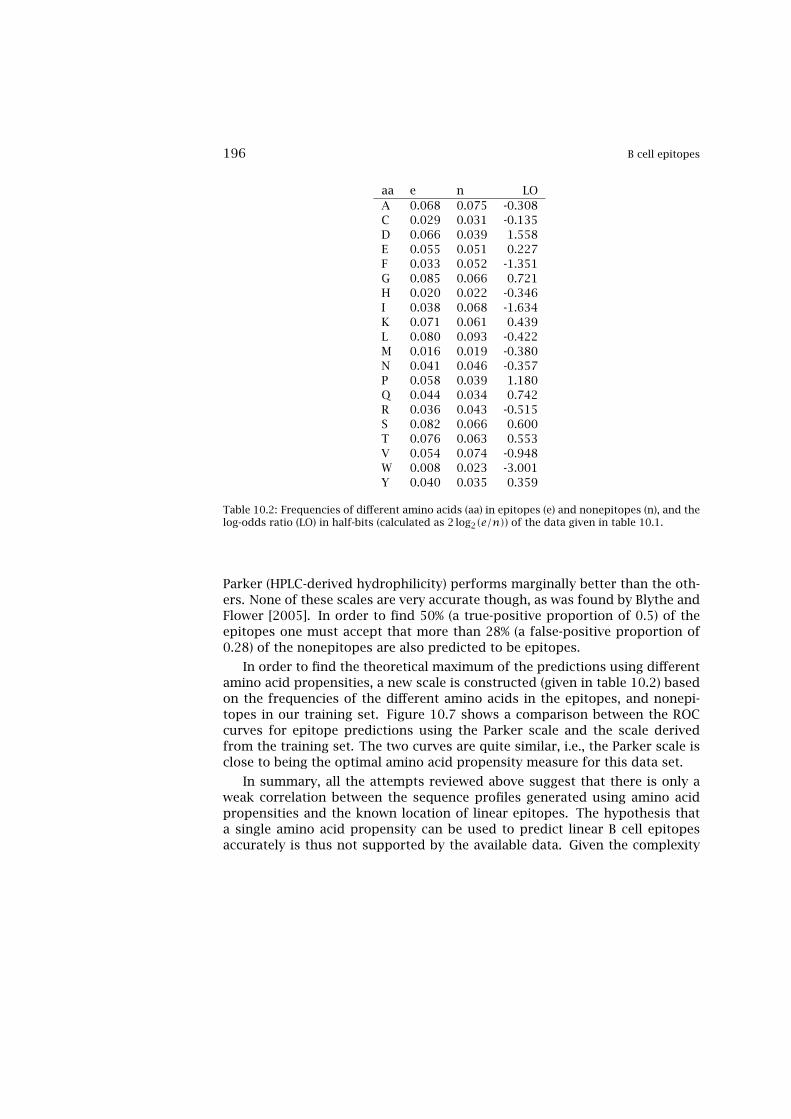
196 B cell epitopes
aa e n LOA 0.068 0.075 -0.308C 0.029 0.031 -0.135D 0.066 0.039 1.558E 0.055 0.051 0.227F 0.033 0.052 -1.351G 0.085 0.066 0.721H 0.020 0.022 -0.346I 0.038 0.068 -1.634K 0.071 0.061 0.439L 0.080 0.093 -0.422M 0.016 0.019 -0.380N 0.041 0.046 -0.357P 0.058 0.039 1.180Q 0.044 0.034 0.742R 0.036 0.043 -0.515S 0.082 0.066 0.600T 0.076 0.063 0.553V 0.054 0.074 -0.948W 0.008 0.023 -3.001Y 0.040 0.035 0.359
Table 10.2: Frequencies of different amino acids (aa) in epitopes (e) and nonepitopes (n), and thelog-odds ratio (LO) in half-bits (calculated as 2 log2(e/n)) of the data given in table 10.1.
Parker (HPLC-derived hydrophilicity) performs marginally better than the oth-ers. None of these scales are very accurate though, as was found by Blythe andFlower [2005]. In order to find 50% (a true-positive proportion of 0.5) of theepitopes one must accept that more than 28% (a false-positive proportion of0.28) of the nonepitopes are also predicted to be epitopes.
In order to find the theoretical maximum of the predictions using differentamino acid propensities, a new scale is constructed (given in table 10.2) basedon the frequencies of the different amino acids in the epitopes, and nonepi-topes in our training set. Figure 10.7 shows a comparison between the ROCcurves for epitope predictions using the Parker scale and the scale derivedfrom the training set. The two curves are quite similar, i.e., the Parker scale isclose to being the optimal amino acid propensity measure for this data set.
In summary, all the attempts reviewed above suggest that there is only aweak correlation between the sequence profiles generated using amino acidpropensities and the known location of linear epitopes. The hypothesis thata single amino acid propensity can be used to predict linear B cell epitopesaccurately is thus not supported by the available data. Given the complexity

Recognition of Antigen by B cells 197
Figure 10.7: ROC curves for epitope predictions using Parker scale [Parker et al., 1986] anda scale derived from the amino acid frequencies of the epitope and nonepitope regions givenin table 10.1 (given in table 10.2 and shown as “bepi” in the legend). Both predictions use awindow of seven, where the central position in the window is the average of seven amino acidpropensities in the window.
of antibody-antigen interactions, this is not a surprising result. Preliminarydata suggest that even a nonlinear prediction method such as a neural net-work does not improve the accuracy of predictions based on single amino acidpropensities significantly. The development of more sophisticated methodsmay be required to predict linear B cell epitopes accurately. One approachwould be to use the sequence to predict the (local) structure of the protein,and use this as input to an epitope prediction algorithm. In the next section,we will see how B cell epitopes can be predicted if the structure of the proteinis available.
10.2.2 Predicting Discontinuous B Cell Epitopes
A major step forward in understanding the nature of the discontinuous epi-topes has been the identification of the antibody-antigen complex structures athigh resolution (see figures 10.4 and 10.3 for examples). Antibodies can onlybind to amino acids which are exposed on the surface of proteins. The surfaceof proteins is normally defined as the atoms which are accessible to water. This
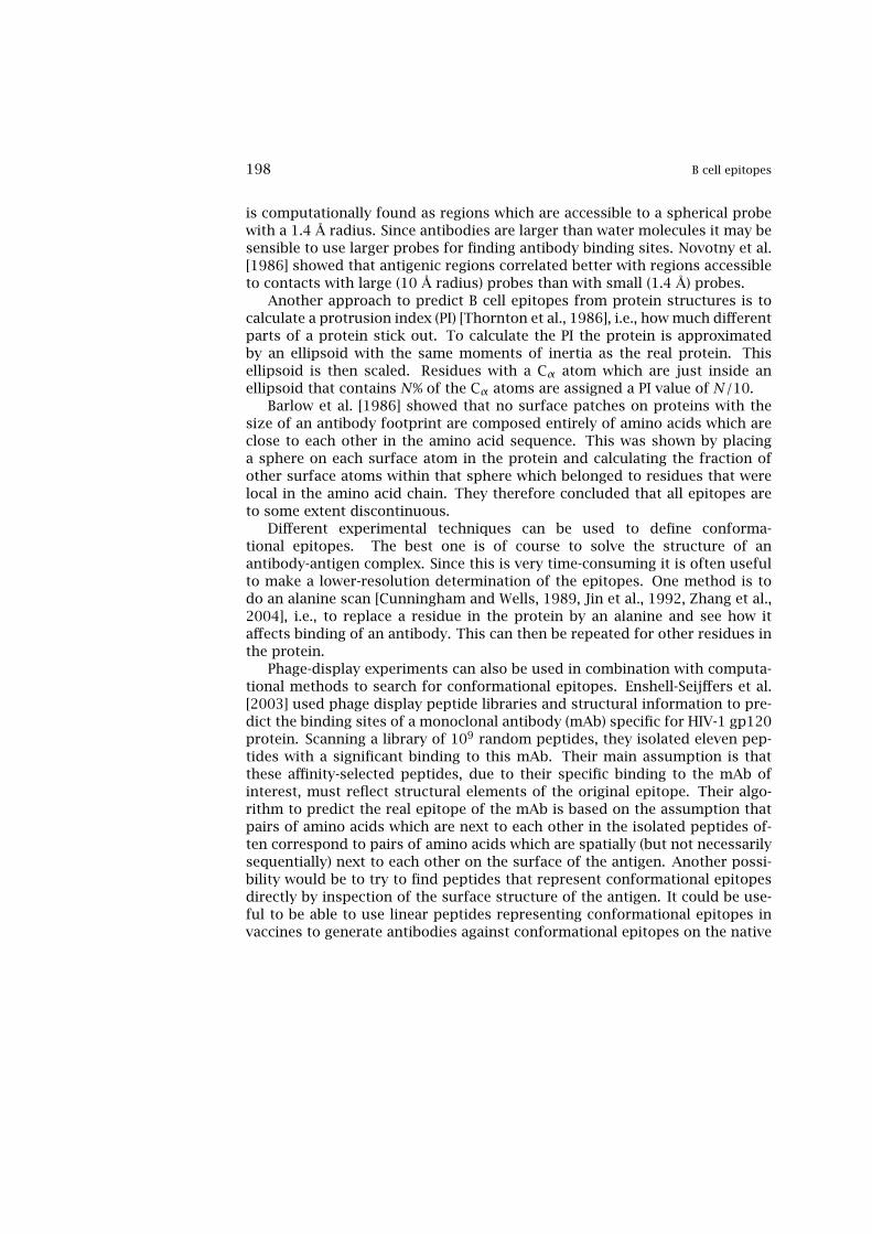
198 B cell epitopes
is computationally found as regions which are accessible to a spherical probewith a 1.4 Å radius. Since antibodies are larger than water molecules it may besensible to use larger probes for finding antibody binding sites. Novotny et al.[1986] showed that antigenic regions correlated better with regions accessibleto contacts with large (10 Å radius) probes than with small (1.4 Å) probes.
Another approach to predict B cell epitopes from protein structures is tocalculate a protrusion index (PI) [Thornton et al., 1986], i.e., how much differentparts of a protein stick out. To calculate the PI the protein is approximatedby an ellipsoid with the same moments of inertia as the real protein. Thisellipsoid is then scaled. Residues with a Cα atom which are just inside anellipsoid that contains N% of the Cα atoms are assigned a PI value of N/10.
Barlow et al. [1986] showed that no surface patches on proteins with thesize of an antibody footprint are composed entirely of amino acids which areclose to each other in the amino acid sequence. This was shown by placinga sphere on each surface atom in the protein and calculating the fraction ofother surface atoms within that sphere which belonged to residues that werelocal in the amino acid chain. They therefore concluded that all epitopes areto some extent discontinuous.
Different experimental techniques can be used to define conforma-tional epitopes. The best one is of course to solve the structure of anantibody-antigen complex. Since this is very time-consuming it is often usefulto make a lower-resolution determination of the epitopes. One method is todo an alanine scan [Cunningham and Wells, 1989, Jin et al., 1992, Zhang et al.,2004], i.e., to replace a residue in the protein by an alanine and see how itaffects binding of an antibody. This can then be repeated for other residues inthe protein.
Phage-display experiments can also be used in combination with computa-tional methods to search for conformational epitopes. Enshell-Seijffers et al.[2003] used phage display peptide libraries and structural information to pre-dict the binding sites of a monoclonal antibody (mAb) specific for HIV-1 gp120protein. Scanning a library of 109 random peptides, they isolated eleven pep-tides with a significant binding to this mAb. Their main assumption is thatthese affinity-selected peptides, due to their specific binding to the mAb ofinterest, must reflect structural elements of the original epitope. Their algo-rithm to predict the real epitope of the mAb is based on the assumption thatpairs of amino acids which are next to each other in the isolated peptides of-ten correspond to pairs of amino acids which are spatially (but not necessarilysequentially) next to each other on the surface of the antigen. Another possi-bility would be to try to find peptides that represent conformational epitopesdirectly by inspection of the surface structure of the antigen. It could be use-ful to be able to use linear peptides representing conformational epitopes invaccines to generate antibodies against conformational epitopes on the native

Neutralizing Antibodies 199
protein.
10.3 Neutralizing Antibodies
Depending on where in an antigen a B cell epitope occurs, the consequences ofantibody binding differ. For example, if an antibody can efficiently block thereceptors mediating infection, the infection rate decreases drastically. Suchantibodies are called neutralizing antibodies (nAbs). A number of studies havesuggested that the induction of nAb responses is critical for virus elimina-tion and protective immunity [Battegay et al., 1993, Planz et al., 1996, Thom-sen et al., 1996, Brundler et al., 1996, Zinkernagel, 1996, Planz et al., 1997,Baldridge et al., 1997]. In infections with cytopathic viruses (viruses that killcells), nAbs are generated within 6 to 14 days, whereas with some viruses likeHIV [Weiss et al., 1985, Robert-Guroff et al., 1985, Moore et al., 1994], HBV[Barnaba et al., 1990], and lymphocytic choriomeningitis virus (LCMV) [Batte-gay et al., 1993], they are not generated until 50 to 150 days have elapsed.Both LCMV and HBV are noncytopathic viruses.
These observations suggest that there is a correlation between the degreeof cytopathic effect and the speed of nAb production. Non-neutralizing anti-bodies appear very early during LCMV and HBV infections; therefore the delayin the nAb response cannot be explained by reduced antigenic stimulus [Batte-gay et al., 1993]. However, nAb–producing B cells do become infected in LCMVand HBV infections, most probably because neutralizing surface immunoglob-ulin might serve as a receptor for the infection [Barnaba et al., 1990, Planzet al., 1996]. The delay may therefore be caused by the elimination of infectedB cells by cytotoxic T cells [Barnaba et al., 1990, Battegay et al., 1993, Planzet al., 1996]. Using a simple mathematical model it is shown that CTLs have atwofold effect on the nAb dynamics: Apart from killing infected B cells [Planzet al., 1996], CTLs also suppress the proliferation of the nAb-producing B cellsby limiting the antigenic stimulus [Kesmir and de Boer, 1998]. Thus, reduc-ing the proliferation rate of nAb-producing B cells, the production of nAb isdelayed in infections with noncytopathic viruses.
To predict which regions of an antigen can induce neutralizing antibodies isone of the ultimate goals of immunological bioinformatics. The mechanism ofneutralization is not fully understood. Early studies suggested that virus neu-tralization was a single-hit mechanism, i.e., that the binding of one antibody toa virus completely neutralized it. This was based on the observation that theinfectivity of viruses declined exponentially (first-order decay) after they weremixed with antibodies, with no lag phase as would be expected if two or moreantibodies had to bind. The first-order decay is, however, also compatible withan incremental neutralization model where each antibody partly neutralizes

200 B cell epitopes
the virus [Icenogle et al., 1983].In a recent review Burton et al. [2001] favor a simple model: In most cases
neutralizing antibodies bind to the surface of the virus and interfere with theattachment of the virus to the target cells or the fusion with it and the neutral-ization is proportional to the number of antibodies bound, no matter whereon the surface they bind. Due to their size and flexibility a bound antibodymay interfere with virus-cell binding within a relatively large area determinedby their reach. For HIV-1, e.g., it has been found that when a fraction f of theantibody binding sites on the gp120 envelope protein is occupied by antibod-ies, the infectivity relative to when no antibodies are bound is approximately(1− f)3. The gp120 molecules sit together three and three (in trimers) on thesurface of HIV-1 and this finding is thus consistent with a model where thebinding of an antibody to one gp120 on the surface of an HIV-1 virion takesout the trimer of gp120 molecules it sits in [Schønning et al., 1999].

Chapter 11
Vaccine Design
Vaccination can broadly be defined as the administration of a substance to aperson with the purpose of preventing a disease. This substance is often akilled or weakened microorganism. Vaccination works by creating a type ofimmune response that enables the memory cells to later respond to a similarorganism before it can cause disease. The earliest documented examples ofvaccinations are from India and China in the 17th century, where vaccinationwith powdered scabs from people infected with smallpox was used to protectagainst the disease. Smallpox used to be a common disease throughout theworld and 20 to 30% of infected persons died from the disease. Smallpox wasresponsible for 8 to 20% of all deaths in several European countries in the18th century [André, 2003]. The tradition of vaccination may have originatedin India in AD 1000 [Plotkin and Orenstein, 1999]. In 1721 Lady Mary Wort-ley Montagu brought the knowledge of these techniques from Constantinople(now Istanbul) to England. Two to three percent of the smallpox vaccinees,however, died from the vaccination itself so it was an important step forwardwhen Benjamin Jesty and, later, Edward Jenner could show that vaccinationwith the less dangerous cowpox could protect against infection with smallpox.This experiment inspired the word vaccination, which is derived from vacca,the Latin word for cow. The vaccination with cowpox (vaccinia) still has seriousside effects and leads to the death of 1 in 10,000 vaccinees. It is possible thatit was the introduction of the smallpox vaccine that was a significant factorin the population growth and improvement in health seen at that time [An-dré, 2001]. Smallpox was officially declared eradicated by WHO in 1980 andvaccination against smallpox was discontinued.
In 1879 Louis Pasteur showed that chicken cholera weakened by growingit in the laboratory could protect against infection with more virulent strains,and in 1881 he showed in a public experiment at Pouilly-Le-Fort that his an-
201

202 Vaccine design
thrax vaccine was efficient in protecting sheep, a goat, and cows. In 1885Pasteur developed a vaccine against rabies based on a live attenuated virus,and a year later Edmund Salmon and Theobald Smith developed a (heat) killedcholera vaccine. Over the next 20 years killed typhoid and plague vaccineswere developed. It was not until 1927 that the next live vaccine was devel-oped: the bacille Calmette-Guérin (BCG vaccine) against tuberculosis.
After the Second World War the ability to make cell cultures, i.e., the abilityto grow cells from higher organisms such as vertebrates in the laboratory,made it easier to develop new vaccines, and the number of pathogens for whichvaccines can be made have almost doubled. Before that time many vaccines,were grown in chicken embryo cells (from eggs), and even today many vaccinessuch as the influenza vaccine, are still produced in eggs, but alternatives arebeing investigated [Mabrouk and Ellis, 2002].
Vaccines have been made for only 34 of the more than 400 knownpathogens that are harmful to man. These are listed in table 11.1. Some ofthe vaccines, however, are not used to their full potential. It is estimatedthat immunization saves the lives of 3 million children each year, but that2 million more lives could be saved if existing vaccines were applied on afull-scale worldwide [André, 2003].
11.1 Categories of Vaccines
Vaccines can be broadly classified into three groups [Ellis, 1999]: live, subunit(killed or inactivated), and genetic.
11.1.1 Live Vaccines
Live vaccines are able to replicate in the host but are attenuated (weakened),i.e., they do not cause disease. They are advantageous because they ofteninduce a broad immune response, low doses of vaccine are sufficient, andthey induce a long-lasting protection [Ellis, 1999, Plotkin and Orenstein, 1999].However, they may cause adverse reactions and they may be transmitted fromperson to person. Many different methods of attenuation have been invented[Ellis, 1999, Plotkin and Orenstein, 1999]. The one most frequently used is apassage in cell culture, i.e., growing the pathogen for many generations in thelaboratory. This technique has been used to develop live vaccines against polioand tuberculosis (BCG). Other attempts to make attenuated vaccines involvethe development of temperature-sensitive mutants which cannot grow at 37◦
C, or reassortant viruses containing genes from two different viruses. Finally,attenuated vaccines can also be made by deleting genes that are responsiblefor virulence by recombinant methods.

Categories of Vaccines 203
Organism Type Vaccine Type YearVariola virus Virus Live 1798Rabies virus Virus Inactivated 1885Salmonella typhi Bacteria Live 1896Vibrio cholerae Bacteria Inactivated 1896Yersinia pestis Bacteria Inactivated 1897Corynebacterium diphtheriae Bacteria Toxoid 1923Bordetella pertussis Bacteria Acellular 1926Clostridium tetani Bacteria Toxoid 1927Mycobacterium tuberculosis Bacteria Live 1927Yellow fever virus Virus Live 1935Influenza virus type A Virus Inactivated 1936Influenza virus type B Virus Inactivated 1936Coxiella burnetii Bacteria Inactivated 1938Rickettsia prowazekii Bacteria Inactivated 1938Rickettsia rickettsii Bacteria Inactivated 1938Central European encephalitis virus Virus Inactivated 1939Poliovirus types 1, 2, and 3 Virus Inactivated/Live 1962Measles virus Virus Live 1963Mumps virus Virus Live 1967Rubivirus Virus Live 1969Staphylococcus aureus Bacteria Staphage lysate 1976Streptococcus pneumoniae Bacteria Polysaccharide 1977Human adenovirus types 4 and 7 Virus Live 1980Neisseria meningitidis Bacteria Polysaccharide 1981Hepatitis B Virus Recombinant 1986Haemophilus influenzae Bacteria Conjugate 1987Hantaan virus Virus Inactivated 1989Japanese encephalitis virus Virus Inactivated 1992Varicella-zoster virus Virus Live 1994Hepatitis A Virus Inactivated 1995Escherichia coli Bacteria Inactivated 1995Junin virus Virus Live 1996Bacillus anthracis Bacteria Adsorbed 1998Borrelia burgdorferi Bacteria Recombinant 1998
Table 11.1: List of diseases for which a vaccine has been made. The table shows the organismname, type (Virus/Bacteria), the vaccine type, and the year the vaccine was invented/licensed.The list have been compiled from FDA [2003], Plotkin and Orenstein [1999], Brooks et al.[2001], Marshall et al. [2003], NIAID [2000], Choi et al. [2003]. The data were extracted fromhttp://www.cbs.dtu.dk/databases/Dodo.
11.1.2 Subunit Vaccines
Subunit vaccines are easier to produce, but they generally induce less CTLresponse than live vaccines, because viral and bacterial proteins are not pro-
204 Vaccine design
duced in the cells of the vaccinated individual. The classic way of makingsubunit vaccines is to inactivate a whole virus or bacterium by heat or by chem-icals. The vaccine may be purified further by selecting one or a few proteinswhich confer protection. This has been done for the Bordetella pertussis vac-cine to create a better-tolerated vaccine that is free from whole microorganismcells [Romanos et al., 1991].
The hepatitis B virus (HBV) vaccine was originally based on the surface anti-gen purified from the blood of chronically infected individuals. Due to safetyconcerns, the HBV vaccine became the first to be produced using recombinantDNA technology [Moss et al., 1984]. It is now produced in bakers’ yeast (Sac-charomyces cerevisiae). Recombinant technologies can also be used to produceviral proteins that self-assemble to viral-like particles (VLPs) with the same sizeas the native virus. VLP is the basis of a promising new vaccine against humanpapilloma virus (HPV) [Marshall et al., 2003].
Many bacteria have polysaccharides in their outer membrane and thesehave been used to make vaccines against Neisseria meningitidis and Strepto-coccus pneumoniae. Polysaccharides generate a T cell-independent responseand this makes them inefficient in children younger than 2 years old. This ob-stacle can be overcome by conjugating these polysaccharides to peptides andthis principle has been used in vaccines against Streptococcus pneumoniae andHaemophilus influenzae [Ellis, 1999].
Toxins are responsible for the pathogenesis of many bacteria. For bacteriasuch as Bordetella pertussis, Clostridium tetani, and Corynebacterium diphthe-riae, vaccines based on inactivated toxins (toxoids) have been developed. Thishas traditionally been done by chemical means but it can now also be done byaltering the DNA sequences that are important for encoding toxicity.
11.1.3 Genetic Vaccines
Genetic vaccines are relatively easy to produce, and they can induce a cellularresponse. One technique to make a genetic vaccine is to inject DNA encodingfor a viral or bacterial protein (also called naked DNA) intramuscularly. Someof the muscle cells will then take up this DNA and will begin to produce theencoded protein. The DNA can also be used to coat small gold particles whichare then shot into the tissue and hence the cell nuclei. Another strategy isto use recombinant strains of viruses or bacteria as so-called vectors to carryepitopes from other pathogens, and thereby vaccinate against these. Mostof the focus within the field of genetic vaccines has been on viruses such asvaccinia, adenovirus, or alphaviruses, and bacteria such as Salmonella typhi orMycobacterium tuberculosis.
Genetic vaccines may also be designed to carry one or more epitopes rather

Polytope Vaccine: Optimizing Plasmid Design 205
than whole proteins. A number of computational methods for identifying spe-cific epitopes have been reviewed in previous chapters. The next chapter willgive an overview of web-based services based on these tools. These can beused to design epitope vaccines [Sette and Fikes, 2003], not only for identifica-tion of the epitopes but also for selecting combinations of them with desiredproperties; e.g., in relation to pathogen variation. Ishioka et al. [1999] suggestthat epitope-based vaccines are advantageous because they can:
• be more potent,
• be controlled better,
• induce subdominant epitopes (e.g. against tumor antigens where thereis tolerance against dominant epitopes),
• target multiple conserved epitopes in rapidly mutating pathogens likeHIV and Hepatitis C virus (HCV),
• be designed to break tolerance,
• overcome safety concerns associated with entire organisms or proteins.
Epitope-based vaccines have been shown to confer protection in animalmodels (see [Snyder et al., 2004] and references in Rodriguez et al. [1998] andSette and Sidney [1999]).
11.1.4 Passive Immunization
The vaccines described above are examples of active immunizations, where anagent is introduced to create a protective immune response. In passive im-munization antibodies are harvested from infected patients or animals andare then used to protect against disease. Passive immunizations are stillused in special cases against many pathogens: cytomegalovirus, hepatitis Aand B viruses, measles, varicella, rubella, respiratory syncytial virus, rabies,Clostridium tetani, varicella-zoster virus, vaccinia, Clostridium botulinum, andCorynebacterium diphtheriae [Marshall et al., 2003].
11.2 Polytope Vaccine: Optimizing Plasmid Design
A short epitope sequence is often capable of inducing protective immunityagainst a large and complex pathogen. Including several such immunogenicepitopes in a “polytope” vaccine construct (reviewed by [Suhrbier, 2002]) mayinduce immunity against multiple antigenic targets, multiple strain variants, or

206 Vaccine design
Sequence Protein Position NameVLAEAMSQV Gag 362 Gag0NTVATLYCV Gag 80 Gag1GLADQLIHL Vif 101 Vif2ILKEPVHGV Pol 476 Pol3SLYNTVATL Gag 77 Gag4
Table 11.2: The five peptides included in the HIV A2 polytope construct. The first column givesthe peptide sequence, the second column the HIV protein the epitope originates from, the thirdcolumn the epitope position in the protein, and the last column the name of the epitope in thepolytope plots (figure 11.1). The five peptides are all known HLA-A2 restricted epitopes [Corbetet al., 2003].
even multiple pathogens. Such an immunization is highly relevant to induceprotection against organisms like HIV and Epstein-Barr virus where immuneescape is an important issue, or for cancer treatment where immunization withsubdominant epitopes might be effective in breaking the tolerance [Suhrbier,1997, Thomson et al., 1998].
Large efforts have been invested in making a proof-of-concept for the poly-tope DNA vaccine approach. Ishioka et al. [1999] have shown that protectiveimmunity against HIV and HBV in HLA transgenic mice can be obtained byimmunizing with a polytope DNA minigene encoding nine dominant CTL epi-topes. Others have obtained similar results for human papilloma virus, HIV,and melanoma [Doan et al., 2005, Woodberry et al., 1999, Mateo et al., 1999].However, as of today no polytope vaccine has been shown to induce protec-tion in humans. “Computational vaccinology” based on quantitative predictionapproaches may help design better polytope vaccines [Flower et al., 2003].
When a polytope is delivered as a DNA vaccine, successful immunizationcan be obtained only if the epitopes encoded by the polytope are correctlyprocessed and presented. Thus, cleavage by the proteasome in the cytosol,translocation into the ER by the TAP complex, as well as binding to MHC classI should be taken into account in an integrative manner. The design of a poly-tope can be done in an effective way by modifying the sequential order of thedifferent epitopes, and by inserting specific amino acids that will favor optimalcleavage and transport by the TAP complex, as linkers between the epitopes.
Here we give an example of an optimized HIV polytope. This polytope isconstructed from five known HLA-A2 restricted epitopes from different HIVproteins [Corbet et al., 2003]. The epitopes are listed in table 11.2.
For simplicity we focus only on the proteasome cleavage and MHC bindingaspects of the antigenic processing and presentation, i.e., we leave out TAPfrom our analysis here. The quality of the polytope can be evaluated in terms

Therapeutic Vaccines 207
of four measures:
1. The number of poor C-terminal cleavage sites of epitopes (predictedcleavage < 0.9)
2. The number of internal cleavage sites (within epitope cleavages with aprediction larger than the predicted C-terminal cleavage)
3. The number of new epitopes (number of processed and presented epi-topes in the fusing regions spanning the epitopes)
4. The length of the linker region inserted between epitopes.
The prediction of proteasomal cleavage and MHC class I binding is doneusing the methods described in chapters 6 and 7. The polytope is optimizedby permutating the order of the epitopes, and by insertion of linker aminoacids in between the epitopes. The optimization seeks to minimize the abovefour terms by use of Monte Carlo Metropolis simulations [Metropolis et al.,1953].
In figure 11.1 a graphical representation of two polytope constructs isshown. The upper figure shows the polytope configuration before optimiza-tion, and the lower figure the polytope after antigen processing and presenta-tion have been optimized. In the initial polytope, the epitopes are placed headto tail in random order (figure 11.1, upper panel). This construct has a rela-tively poor predicted antigenic processing and presentation score: one of theepitopes (Gag-0) has a poor C-terminal cleavage score, three epitopes (Gag-0,Gag-1, and Gag-4) have strong internal cleavage sites (one epitope, Gag-1, hasfour internal cleavage sites), and one new epitope is predicted in the fusion re-gion spanning two epitopes (Gag-0 and Gag-1). After the polytope optimization(figure 11.1, lower panel) all epitopes have a strong C-terminal cleavage, onlyone internal cleavage site remains (in Gag-1), and no new epitopes appear inthe fusion regions. It thus seems natural to expect that the optimized polytopeconstruct should have a high chance of presenting all five epitopes, and hencea higher chance of inducing immunity. A natural extension of the outlinedapproach will be to include the TAP transport efficiency in the optimizationprocedure.
11.3 Therapeutic Vaccines
Vaccines are normally administered to healthy individuals to prevent disease.Nevertheless, there is a growing trend to use vaccines to treat the patients thatalready have a disease. Efforts are being devoted to developing therapeuticvaccines against tumors, AIDS, allergies, autoimmune diseases, hepatitis B,
208 Vaccine design
Figure 11.1: Two configurations of the HIV A2 polytope. The upper panel shows the initialconfiguration with the epitopes placed head to tail in a random manner. The lower panel showsthe optimized polytope construct. In each panel (A) gives the predicted proteasomal cleavage,and (B) the epitope sequences (in blue), the location of new predicted epitopes (in red). The unitson the x-axis are arbitrary; 1k corresponds to one amino acid. See plate 21 for color version.

Therapeutic Vaccines 209
tuberculosis, malaria, and, possibly, against the bacteria that cause gastriculcers. The idea behind a therapeutic vaccine against autoimmune diseasesand allergy is to suppress an already existing immunity, while vaccines forcancer and persistent infections aim to boost the existing immunity or inducenew immune responses.
11.3.1 Cancer Vaccines
The aim of using a cancer vaccine is to break the tolerance of the immune sys-tem against tumors. Therapeutic cancer vaccines can be classified into threegroups. The first group consists of polyvalent vaccines that can be composedof whole tumor cells, peptides derived from tumor cells in vitro, or heat shockproteins prepared from autologous tumor cells (for a review, see Ragupathiand Livingston [2002]). The second group is tumor-specific antigen–definedvaccines. These vaccines are probably the most difficult ones to develop, aseach individual tumor can have a unique collection of antigens. Mutations caneasily accumulate in tumor cells due to high proliferation rates. Therefore, theinvestigators search for antigens with three main characteristics: (1) maximalimmunogenicity, (2) wide expression by different tumor types, and (3) maxi-mal tumor specificity, i.e., minimal expression in healthy cells [Mocellin et al.,2004]. The last group of cancer vaccines aim to increase the amount of den-dritic cells (DCs) that can initiate a long-lasting T cell response against tumors.Tumor-DC hybrids, or DCs loaded with peptides, whole tumor cells, or tumorRNA, are used as agents in this class of vaccines.
Obviously, not all of these trials are leading to the desired results, but,there are sufficient data to support the notion that therapeutic cancer vaccinescan induce antitumor immune responses in humans with cancer (for a review,see [Lewis, 2004]). Antigenic variation is a major problem that therapeuticvaccines against cancer face. The tools from genomics and bioinformaticscan provide ways to circumvent these problems. First, one can use sequenceanalysis (chapter 3) and diversity measures (chapter 4) to identify the mostconserved protein regions from a specific tumor with least similarity to otherhuman proteins. Then the polytope approach explained above can be usedto generate cancer vaccines from these conserved epitopes specific for tumorcells.
11.3.2 Allergy Vaccines
Immunotherapeutic vaccines against allergies represent an area which has re-ceived much attention lately due to the increasing occurrence of allergies inindustrialized countries. The traditional approach is to vaccinate with small

210 Vaccine design
doses of purified allergen, i.e., induce tolerance. Second-generation vaccinesare under development based on recombinant technology. One promising vac-cine candidate developed by Niederberger et al. [2004] uses genetically engi-neered derivatives of Bet v 1 protein, which is the main cause of birch pollenallergy (see figure 10.4 for the structure of this protein). More than 100 millionpeople world-wide are effected by this allergen. Patients having pollen allergyoften have large amounts of IgE antibodies specific for Bet v 1 protein. Whenexposed to pollen, the IgE-Bet v 1 complexes are formed on the surface of mastcells and basophils. This initiates a series of cellular reactions that cause in-flammation [Kinet, 1999]. Immunization with the derivatives of Bet v 1 inducesa strong IgG antibody response specific for allergen Bet v 1. IgG antibodies donot bind to mast cells and basophils; instead they can efficiently clear the al-lergen, Bet v 1, before IgE-allergen complexes are formed. This results in aten-fold reduction in inflammation caused by basophils [Niederberger et al.,2004]. Moreover, IgG antibodies induced by the vaccine are also specific forBet v 1 cross-reactive allergens, i.e., the vaccine can suppress allergy to relatedpollens.
It is well established that contact with seasonal allergens induces a strongIgE memory response that causes the symptoms to repeat year after year (see,e.g., [Durham et al., 1997]). Therefore, another desired effect of the therapeu-tic vaccine against allergies is to reduce this memory response, so that in thecoming allergen-rich seasons the patient remains symptom-free even withoutthe repeated vaccination. Niederberger et al. [2004] show that genetically en-gineered Bet v 1 vaccine can also reduce pollen-specific IgE memory responsesignificantly. In short, this vaccine is a good example of switching a “wrong”immune response to a less harmful one.
11.3.3 Therapeutic Vaccines against Persistent Infections
The effort to develop this group of vaccines has been blooming recently, es-pecially for preventing HIV-related disease progression. Most of the first can-didate HIV-1 vaccines were based entirely or partially on envelope proteins toboost neutralizing antibodies (see chapter 10). However, these vaccines havenot been successful [Cohen, 2003], because the envelope proteins are the mostvariable parts of the HIV genome [Gaschen et al., 2002], and because they werecomposed of monomeric gp120 molecules that induce antibodies that did notbind to trimeric gp120 on the surface of the virions. A number of recentvaccines are also designed to induce strong cell-mediated responses. These in-clude vaccines based on several different viral vectors with or without primingwith DNA or a recombinant antigen (see, e.g., [Shiver et al., 2002]).
The huge potential for immune escape by HIV remains the major problem
Vaccine Market 211
for the HIV vaccines. Escapes from CTL responses are associated with dis-ease progression and high viral loads [Leslie et al., 2004, Friedrich et al., 2004].While some CTL epitopes escape recognition quickly because they are not func-tionally constrained, others might need several compensatory mutations. Thisis because the latter group of epitopes lie in functionally or structurally con-strained regions of HIV-1. The p24 capsid protein, e.g., is known to be oneof the most conserved proteins of HIV-1 [Novitsky et al., 2002, Leslie et al.,2004, Gaschen et al., 2002]. P24 is part of the Gag protein complex, whichcontrols the assembly of HIV-1 virions and plays a crucial role in the entryto target cells [Gottlinger, 2001, Adamson and Jones, 2004]. P24 contains astretch of 20 residues, which is conserved across all retroviruses and is essen-tial for viral assembly, maturation, and infectivity [Gamble et al., 1997]. It hasbeen shown that most of the capsid surface cannot tolerate point mutationswithout a severe loss of viral fitness [von Schwedler et al., 2003, Leslie et al.,2004]. In contrast, the Nef protein is known to be polymorphic, and duringacute infection immune responses to Nef are typically replaced by responsesto more conserved regions of HIV-1 [Lichterfeld et al., 2004].
11.3.4 Vaccines against Autoimmune Diseases
The biggest success story for therapeutic vaccines was achieved against mul-tiple sclerosis, an autoimmune disease where T cells specific for mylein basicprotein (MBP) can cause inflammation of the central nervous system. The vac-cine uses copolymer 1 (cop 1), a protein that highly resembles MBP. Cop 1competes with MBP in binding to MHC class II molecules, but it is not effec-tive in inducing a T cell response (reviewed by [Kipnis and Schwartz, 2002]).On the contrary, cop 1 can induce a suppressor T cell response specific forMBP, and this response helps diminish the symptoms of multiple sclerosis. In-spired by this example, a vaccine based on the same mechanisms is developedfor myasthenia gravis [Sela and Mozes, 2004].
11.4 Vaccine Market
The vaccine market has increased fivefold from 1990 to 2000, but with annualsales of 6 billion euros it is still less than 2% of the total pharma market. Themajor producers are GlaxoSmithKline (GSK), Merck, Aventis Pasteur, Wyeth,and Chiron who have 85% of the market. The main products are hepatitis B,flu, MMR (measles, mumps, and rubella) and DTP (diphtheria, tetanus, pertus-sis) vaccines which represent more than half the market. Of these 40% areproduced in the United States and the rest is evenly split between Europe andthe rest of the world [Gréco, 2002]. It currently costs between 200 and 500

212 Vaccine design
million US dollars to bring a new vaccine from the concept stage to market[André, 2002].

Chapter 12
Web-Based Tools for VaccineDesign
In classic immunological research, results could be recorded by pen and paperor in a spreadsheet, but new experimental high-throughput methods such assequencing, DNA arrays, and proteomics have generated a wealth of data thatcannot be efficiently handled and mined by classic approaches. The field ofimmunological bioinformatics has been growing rapidly in the past years toprovide accurate methods for analysis of emerging immunological data. Manyof the methods have been made available on the Internet and can be used byexperimental researchers without expert knowledge of bioinformatics. Thischapter attempts to give an overview of the methods currently available andto point out the strengths and weaknesses of the different methods.
12.1 Databases of MHC Ligands
Several databases of MHC binding peptides now exist on the web (see table12.1).
SYFPEITHI: The SYFPEITHI database contains information on peptide se-quences, anchor positions, MHC specificity, source proteins, source organisms,and references to publications. The database has more than 4000 peptide se-quences known to bind MHC class I and class II molecules and is based onprevious publications on T cell epitopes and MHC ligands from many species[Rammensee et al., 1999].
MHCPEP: The other major database of peptides that bind MHC is theMHCPEP database [Brusic et al., 1998a]) which comprises over 13.000 peptidesequences known to bind MHC molecules. Entries were compiled from pub-
213

214 Web-based tools for vaccine design
Name Principal Investigators URL DescriptionSYFPEITHI Rammensee www.syfpeithi.de/ Natural MHC ligandsMHCPEP Brusic, Harrison wehih.wehi.edu.au/mhcpep MHC binding peptidesJenPep Flower www.jenner.ac.uk/jenpep2 MHC and TAP ligands, B cell epitopesMHCBN Raghava www.imtech.res.in/raghava/mhcbn Tools for subunit vaccine designHLA ligand/motif Hildebrand hlaligand.ouhsc.edu Ligand database/predictionDatabaseHIV molecular Korber hiv-web.lanl.gov/content/ HIV epitopesimmunology database immunology/EPIMHC Reinherz immunax.dfci.harvard.edu/Tools/ MHC ligands
db_query_epimhc.html
Table 12.1: Databases of MHC binding peptides.
lished reports as well as from direct submissions of experimental data. Eachentry contains the peptide sequence, its MHC specificity, and, when available,experimental method, observed activity, binding affinity, source protein, an-chor positions, and publication references. Unfortunately, the database has,since June 1998, been static. The database can be downloaded as an ASCII file.
JenPep: The JenPep database is a newer database that contains quantitativebinding data of peptides to MHC and TAP, as well as B and T cell epitopes[Blythe et al., 2002]. The database contains more than 8000 entries.
MHCBN: MHCBN [Bhasin et al., 2003] is a database of MHC binding and non-binding peptides containing 17,129 binders, and 2648 nonbinders for morethan 400 MHC molecules.
HLA Ligand/Motif Database: This site contains a database that can besearched by defining allele and specificity, amino acid pattern, ligand/motifin sequence of amino acids, author’s last name, or advanced search with morecriteria [Sathiamurthy et al., 2003].
HIV Molecular Immunology Database: The HIV molecular immunologydatabase is an annotated, searchable collection of HIV-1 cytotoxic and helperT cell epitopes and antibody binding sites. The goal of the database is toprovide a comprehensive listing of well-defined HIV-1 epitopes [Korber et al.,2001a].
EPIMHC: An MHC ligand database that can be searched based on sequence,length, class, species, and on whether a ligand is an epitope or not.
NIH has this year started an immune epitope database (IEDB) and analysisprogram (www2.niaid.nih.gov/Biodefense/Research/resources.htm#immepi)to design, develop, populate, and maintain a publicly accessible, compre-hensive immune epitope database containing linear and structural antibodyepitopes and T cell epitopes. This database may eventually incorporatemost of the data from the above described databases. It will be available atwww.immuneepitope.org/.

Prediction Servers 215
Name URL DescriptionBIMAS bimas.dcrt.nih.gov/molbio/hla_bind Prediction of MHC class I binding using matricesSYFPEITHI www.syfpeithi.de/ Prediction of MHC class I and II bindingPREDEPP bioinfo.md.huji.ac.il/ MHC class I epitope prediction
marg/Teppred/mhc-bindEpipredict www.epipredict.de/ Prediction of HLA class II restricted bindingProPred www.imtech.res.in/raghava/propred MHC class II predictionMHCPred www.jenner.ac.uk/MHCPred HLA class I predictionsNetMHC www.cbs.dtu.dk/services/NetMHC-2.0 Prediction of HLA class I
binding using ANNs and HMMsLpPep zlab.bu.edu/zhiping/lppep.html Prediction of HLA-A2 bindingMAPPP www.mpiib-berlin.mpg.de/ Registration needed for expert model.
MAPPP/expertquery.htmlCombined open reading frame, MHC binding, andproteasomal cleavage
Table 12.2: Servers for predicting binding of peptides to MHC molecules.
12.2 Prediction Servers
12.2.1 Prediction of MHC Binding
Several peptide-MHC binding prediction servers exist on the web (table 12.2).As indicated in the table some of the web-based methods also allow predic-tion of binding to MHC class II molecules. Most methods available on the webfor predicting MHC-peptide binding are matrix methods. Matrices or hiddenMarkov models (HMMs) may be derived from a set of ligand sequences as de-scribed in chapter 4. In these methods the amino acid on each position inthe motif gives an independent contribution to the prediction score. Neuralnetworks can generate more accurate predictions if correlations between po-sitions exist, and if there are enough data to train a neural network properly.
BIMAS: The BIMAS method was developed by Parker et al. [1994]. Themethod is based on coefficient tables deduced from the published literature.For HLA-A2, peptide binding data were combined together to generate a ta-ble containing 180 coefficients (20 amino acids x 9 positions), each of whichrepresents the contribution of one particular amino acid residue at a specifiedposition within the peptide [Parker et al., 1994].
SYFPEITHI: The SYFPEITHI predictions are based on published motifs (poolsequencing, natural ligands) and take into consideration the amino acids inthe anchor and auxiliary anchor positions, as well as other frequently occur-ring amino acids within a binding motif. The score is calculated according tothe following rules: Each residue in a certain peptide is given a specific valuedepending on whether it occurs in an anchor or auxiliary anchor position, orif it is one of the preferred residues. Ideal anchors will be given 10 points,unusual anchors 6 to 8 points, auxiliary anchors 4 to 6 points, and preferredresidues 1 to 4 points. Amino acids that are regarded as having a negativeeffect on the binding ability are given values between -1 and -3 [Rammenseeet al., 1995, 1999]. On the SYFPEITHI website predictions can be made for 6
216 Web-based tools for vaccine design
different MHC class II alleles and 21 MHC class I alleles.PREDEPP: In this method the peptide structure in the MHC groove is used
as a template upon which peptide candidates are threaded, and their compat-ibility to bind is evaluated by statistical pairwise potentials. This method hasthe advantage that it does not require experimental testing of peptide binding,and can thus be used for alleles where only few data are available [Schueler-Furman et al., 2000].
Epipredict: This server is based on a method that uses synthetic combina-torial peptide libraries to describe peptide-HLA class II interaction in a quanti-tative way. The binding contribution of every amino acid side chain in an MHCclass II ligand is described by allele-specific 2D databases [Jung et al., 2001].
ProPred: The ProPred method [Singh and Raghava, 2001] is based on thematrices published by Sturniolo et al. [1999], and is an implementation andextension of the TEPITOPE program [Hammer, 1995, Raddrizzani and Hammer,2000].
MHCPred: Prediction of binding to 11 different HLA class I alleles and3 HLA class II alleles using a 3D quantitative structure-activity relationshipmethod [Guan et al., 2003].
NetMHC: Prediction of HLA class I binding using neural networks andweight matrices [Buus et al., 2003, Nielsen et al., 2003, 2004]. NetMHC in-cludes allele-specific weight-matrix predictions for more than 120 HLA alleles,and artificial neural network (ANN) and weight matrix predictions for 12alleles representing 12 distinct HLA supertypes. The neural network methodshave been trained using quantitative binding data generated by an ELISAassay [Sylvester-Hvid et al., 2002], and predict the binding affinity. They thusdiffer from methods performing classification only (binding vs. nonbindingaccording to a threshold).
LpPep: A new method for predicting high affinity MHC-binding peptidesbased on linear programming [Peters et al., 2003b].
Two well-known prediction methods, TEPITOPE and EpiMatrix [Meisteret al., 1995, de Groot et al., 1997] that are not available through the web arelisted in table 12.3. TEPITOPE is popular since it allows prediction of peptidesof many different class II molecules. Another prediction method, PREDICT, forMHC class I, II, and TAP binding from the Brusic group [Yu et al., 2002] is alsonot available through the web at the moment.
12.2.2 Prediction of Proteasomal Cleavage Sites
Different methods for predicting proteasomal cleavage sites exist on the web(table 12.4).

Prediction Servers 217
Name URL DescriptionTEPITOPE www.vaccinome.com PC program for class II
predictions can be downloadedEpiMatrix epivax.com/epimatrix.html Commercial epitope predictionPredict Prediction of class I, II, and TAP binding
Table 12.3: MHC binding predictions not publicly available on the Internet.
Name URL DescriptionPaProC paproc.de A matrix-based method for
protasomal cleavage predictionMAPPP www.mpiib-berlin.mpg.de/ Proteolytic fragment predictor
MAPPP/cleavage.htmlNetChop www.cbs.dtu.dk/ A neural–network based
services/NetChop protasomal cleavage predictionbioinfo.md.huji.ac.il/marg/cleavage/ Matrix score to predict
proteasomal cleavage
Table 12.4: Prediction of proteasomal cleavage sites.
PAProC (Prediction algorithm for proteasomal cleavages) is a predictiontool for cleavages by human and yeast proteasomes, based on experimentalcleavage data [Kuttler et al., 2000, Nussbaum et al., 2001]. An updated versionof the PAProC program based on in vitro immunoproteasome cleavage data[Toes et al., 2001] is also in the making according to the PAProC homepage.
MAPPP comprises two different algorithms. One aims at predictingpotential proteasomal cleavage, based on a statistical analysis of cleavage-determining amino acid motifs present around the scissile bond [Holzhutteret al., 1999]. The second algorithm, which uses the results of the cleavagesite analysis as an input, provides predictions of major proteolytic fragments[Holzhutter and Kloetzel, 2000].
NetChop [Kesmir et al., 2002] is a method based on neural networks thathave been trained on different data sets. The network, which was trained onC-terminal cleavage sites of 1110 publicly available MHC class I ligands, per-forms best in predicting the boundaries of CTL [Saxova et al., 2003]. The speci-ficity of this network may resemble the specificity of the immunoproteasome.NetChop3.0 is now available [Nielsen et al., 2005].
The parameters of Altuvia and Margalit [2000] analysis are also recentlyavailable on the net. Another method based on support vector machines canbe found at www.imtech.res.in/raghava/pcleavage.

218 Web-based tools for vaccine design
Figure 12.1: The growth in the number of known MHC sequences and MHC ligands. The graphis adopted from the IMGT/HLA database (www.ebi.ac.uk/imgt/hla/). Notice the exponentialgrowth in the number of MHC alleles (sequences) compared to more or less stable levels ofknown MHC ligands.
12.2.3 Combined Predictions
The MAPPP server (table 12.2) allows the user to make an open reading frame(ORF) search combined with MHC binding and proteasomal cleavage site pre-dictions.
12.2.4 TAP Predictions
The only web-based prediction tool for TAP binding was developed byBhasin and Raghava [2004] and is based on support vector machines(www.imtech.res.in/raghava/tappred).
12.2.5 MHC Sequence Databases
A number of databases containing sequences of proteins of immunologicalinterest exist on the web (table 12.5).
IMGT/HLA: The HLA sequence database currently contains 1156 MHC classI and 712 class II alleles. There are also 11 TAP molecules and 54 MICA se-quences. Figure 12.1 shows the growth of this database in time.
IMGT: IMGT, the international ImMunoGeneTics project, is a collection ofdatabases specializing in immunoglobulins, T cell receptors, and the MHC ofall vertebrate species. The IMGT project was established in 1989 by the Uni-versité Montpellier II and the CNRS (Montpellier, France) and works in close
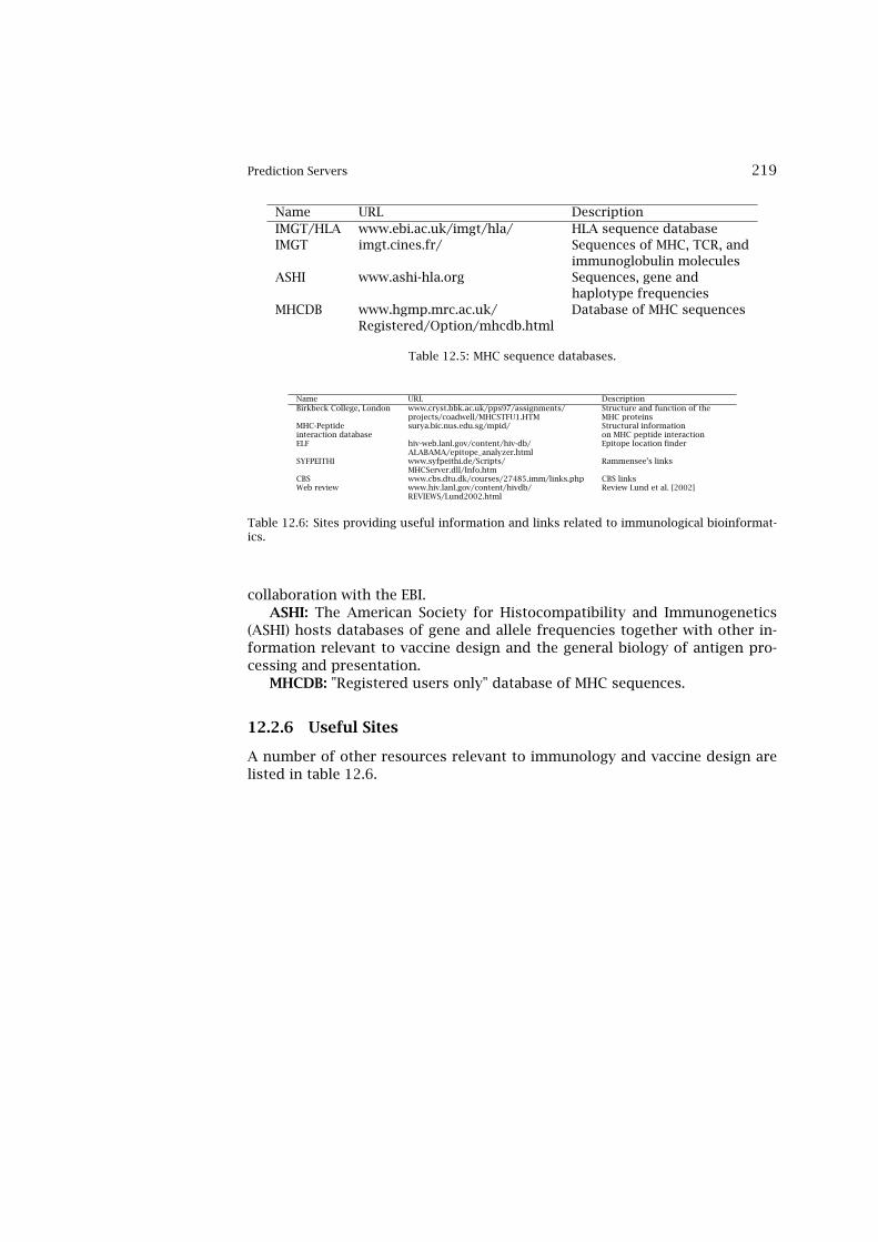
Prediction Servers 219
Name URL DescriptionIMGT/HLA www.ebi.ac.uk/imgt/hla/ HLA sequence databaseIMGT imgt.cines.fr/ Sequences of MHC, TCR, and
immunoglobulin moleculesASHI www.ashi-hla.org Sequences, gene and
haplotype frequenciesMHCDB www.hgmp.mrc.ac.uk/ Database of MHC sequences
Registered/Option/mhcdb.html
Table 12.5: MHC sequence databases.
Name URL DescriptionBirkbeck College, London www.cryst.bbk.ac.uk/pps97/assignments/ Structure and function of the
projects/coadwell/MHCSTFU1.HTM MHC proteinsMHC-Peptide surya.bic.nus.edu.sg/mpid/ Structural informationinteraction database on MHC peptide interactionELF hiv-web.lanl.gov/content/hiv-db/ Epitope location finder
ALABAMA/epitope_analyzer.htmlSYFPEITHI www.syfpeithi.de/Scripts/ Rammensee’s links
MHCServer.dll/Info.htmCBS www.cbs.dtu.dk/courses/27485.imm/links.php CBS linksWeb review www.hiv.lanl.gov/content/hivdb/ Review Lund et al. [2002]
REVIEWS/Lund2002.html
Table 12.6: Sites providing useful information and links related to immunological bioinformat-ics.
collaboration with the EBI.ASHI: The American Society for Histocompatibility and Immunogenetics
(ASHI) hosts databases of gene and allele frequencies together with other in-formation relevant to vaccine design and the general biology of antigen pro-cessing and presentation.
MHCDB: "Registered users only" database of MHC sequences.
12.2.6 Useful Sites
A number of other resources relevant to immunology and vaccine design arelisted in table 12.6.


Chapter 13
MHC Polymorphism
As a result of fast evolution (thanks to the short generation time of microor-ganisms), hosts are under constant selection pressure to invent processes thatcounteract pathogenic invasion. Since the generation time of the vertebratehost is much longer than that of pathogens, obviously the evolution of thehost has a much slower pace. The polymorphism of the MHC molecules isone result of this coevolution between the host and its pathogens. The poly-morphism is one of the major reasons why mammalian organisms cannot beeradicated by infections by a single pathogen: Pathogens that escape from pre-sentation by the MHC molecules of one individual may not be able to escapethe presentation by another individual carrying a different MHC molecule.
13.1 What Causes MHC Polymorphism?
Although there have been extensive debates over the selection pressures lead-ing to the high polymorphism of MHC molecules, there is still not a widelyaccepted model for a mechanism (see Apanius et al. [1997] for a detailed re-view). The common view is that MHC polymorphism arises because of theheterozygote advantage. Different MHC molecules bind different peptides,and thus present different parts of a pathogen to T cells. If a host is heterozy-gous in its MHC loci, it can thus provide a broader immune response, whichin turn would make pathogenic adaptation more difficult. This theory, knownas the theory of overdominance or heterozygote advantage [Hughes and Nei,1988, 1989, 1992], is supported by recent studies on HIV-1 patients. Carring-ton and O’Brien [2003] have reviewed data showing that the degree of MHCheterozygocity correlates with a delayed onset of progress to AIDS.
There exist a number of mathematical models focusing on the heterozy-
221
222 MHC polymorphism
gous advantage as the main reason for MHC polymorphism. Work in the gen-eral area of population genetics models suggests that the heterozygous advan-tage is sufficient to explain the high MHC polymorphism observed in severalMHC loci [Maruyama and Nei, 1981, Takahata and Nei, 1990, Hughes and Yea-ger, 1998]. These models assume that all heterozygous individuals would havethe same fitness (higher than the homozygous individuals) irrespective of theMHC molecules that they harbor. This is, however, an unrealistic assump-tion, as it is now well established that different MHC alleles show differentdegrees of protection to specific pathogens [van Eden et al., 1980, Klein et al.,1994, Hill et al., 1991]. de Boer et al. [2004] show that when the classic pop-ulation genetics models are corrected for this unrealistic assumption, it is nolonger possible to obtain more than 10 alleles per loci. Thus, the heterozy-gous advantage alone cannot explain the large MHC polymorphism observedin mammalian (and most vertebrate) populations.
An additional mechanism that could enlarge MHC polymorphism isfrequency-dependent selection by host-pathogen coevolution. Since it is agood strategy for pathogens to adapt to the most common MHC alleles ina population, the rare alleles would have a selective advantage. This will intime cause the frequency of rare alleles to increase, and the common alleleswill become rare. The dynamic picture arising from this scenario resemblesthe well known principle of red-queen dynamics from ecology [van Valen,1973]. The studies of the snail-trematode parasite system support that such afrequency-dependent selection can take place in nature, as in this system theparasite evolves to become most virulent in the dominant host genotype. Forhumans HIV-1 is an example of a rapidly adapting pathogen to most commonMHC alleles in the population [Trachtenberg et al., 2003, Scherer et al., 2004].
The relative role of frequency-dependent selection and heterozygote ad-vantage is discussed extensively in the literature [Lewontin et al., 1978, Aoki,1980, Hughes and Nei, 1988, 1989]. Recently Borghans et al. [2004] and Belt-man et al. [2002] have developed a computer simulation model of coevolvinghosts and pathogens to study the relative impact of these two mechanisms.This model shows that 1) the frequency-dependent selection scenario alonecan account for the existence of at least 50 alleles per MHC loci, and 2) if thehost population size is large enough, the MHC polymorphism does not be-come too dynamic, i.e., a large set of MHC alleles can persist over many hostgenerations even though host MHC frequencies change continuously.
Many other factors such as MHC-dependent mate selection, geographic andsocial isolation, and strong selection pressures by severe infections (popu-lation “bottlenecks”) can influence the degree of MHC polymorphism arisingin a population. The chimpanzee species is in this respect very interesting:de Groot et al. [2002] have shown that almost any chimpanzee gene is morepolymorphic than human genes, probably because the chimpanzee is an older

MHC Supertypes 223
species. However, the polymorphism of MHC genes seems to be much lowerthan in humans, possibly due to a strong selection pressure caused by simianimmunodeficiency virus (SIV) infection. Even though host-pathogen evolutionseems to be sufficient to explain the large MHC polymorphism [Borghans et al.,2004, Beltman et al., 2002], all other factors mentioned here, together withfrequency-dependent selection, generate the MHC polymorphism we observein many vertebrate populations today.
13.2 MHC Supertypes
The previous section reviewed factors that play a role in generating extremelypolymorphic MHC genes. This polymorphism, although very essential to pro-tect a population from invasion by pathogens, generates a major drawbackfor epitope-based vaccines, which otherwise, from many perspectives, are themost promising vaccine candidates (see chapter 11).
Each MHC molecule has a different specificity. If a vaccine needs to containa unique peptide for each of these molecules it will need to comprise hundredsof peptides. One way to counter this is to select sets of a few HLA moleculesthat together have a broad distribution in the human population. Gulukotaand DeLisi [1996] compiled lists with 3, 4, and 5 alleles which give the maximalcoverage of different ethnic groups. One complication they had to deal withis that HLA alleles are in linkage disequilibrium, i.e., the joint probability ofan allelic pair may not be equal to the product of their individual frequencies,(P(a)P(b) ≠ P(ab)). This means that it is not necessarily optimal to choosethe alleles with the highest individual frequencies. Moreover, Gulukota andDeLisi [1996] find that populations like the Japanese, Chinese, and Thais canbe covered by fewer alleles than the North American black population whichturns out to be very diverse. Thus different alleles should be targeted in orderto make vaccines for different ethnic groups or geographic regions.
A factor that may reduce the number of epitopes necessary to include in avaccine is that many of the different HLA molecules are not functionally differ-ent, i.e., they have similar specificities. The different HLA molecules have beengrouped together in what is called supertypes [Del Guercio et al., 1995, Sidneyet al., 1995, Sette and Sidney, 1999]. This means ideally that if a peptide canbind to one allele within a supertype, it can bind to all alleles within that su-pertype. In practice, however, only some peptides that bind to one allele in asupertype will bind to all alleles within that supertype. A number of differentcriteria have been used to define these supertypes, including structural sim-ilarities, shared peptide binding motifs, identification of cross-reacting pep-tides, and ability to generate methods that can predict cross-binding peptides[Sidney et al., 1996]. For HLA class I molecules Sette and Sidney [1999] de-
224 MHC polymorphism
fined nine supertypes (A1, A2, A3, A24, B7, B27, B44, B58, B62) which werereported to cover most of the HLA-A and -B polymorphisms. They arguedthat the different alleles within each of these supertypes have almost identicalpeptide-binding specificity. They found that while the frequencies at which thedifferent alleles were found in different ethnic groups were very different, thefrequencies of the supertypes were quite constant. Assuming Hardy-Weinbergequilibrium (i.e., infinitely large, random mating populations free from outsideevolutionary forces), they found that more than 99.6% of persons in all ethnicgroups surveyed possessed at least one allele within at least one of these su-pertypes. They also showed that the smaller collections of supertypes A2, A3,B7 and A1, A2, A3, B7, A24, and B44 covered in the range of 83.0 to 88.5%and 98.1 to 100.0% of persons in different ethnic groups, respectively. Threealleles, A29, B8, and B46, were found to be outliers with a different bindingspecificity than any of the supertypes. These may define supertypes them-selves when the specificity of more HLA molecules is known.
Some work has also been done to define supertypes of class II molecules. Ithas been reported that 5 alleles from the DQ locus (DQ1, DQ2, DQ3, DQ4, DQ5)cover 95% of most populations [Gulukota and DeLisi, 1996]. It has also beenreported that a number of HLA-DR types share overlapping peptide-bindingrepertoires [Southwood et al., 1998].
There are recently developed bioinformatical approaches to identificationof HLA supertypes [Lund et al., 2004, Reche and Reinhertz, 2004] defining anovel measure for the difference in the specificities of different HLA moleculesand using the measure to revise the HLA class I supertypes. In the work ofLund et al. [2004] also MHC supertypes for class II molecules are defined, us-ing published specificities for a number of HLA-DR types. This work will bedescribed in detail below.
13.2.1 A Novel Method to Cluster MHC Binding Specificities
In the first part of this section we will be dealing with how to cluster HLA ClassI alleles into supertypes. The basic idea behind the approach is to constructweight matrices of binding peptides as described in chapters 6 and 8, and thenuse these matrices as a representation of the binding specificity of a givenallele. Then all the matrices are compared and clustered by their similarity inthe binding space. This is a powerful alternative to clustering based on MHCsequence similarities.
First, a data set of alleles and their binding peptides is needed: The dif-ferent class I molecules used in this example can be seen in table 13.1. Thecorresponding HLA ligands were extracted from the SYFPEITHI [Rammenseeet al., 1995, 1999] and MHCPEP [Brusic et al., 1998a] databases. All lines con-

MHC Supertypes 225
taining amino acid information were treated as sequences and blanks werereplaced by X. For each allele, weight matrices were built using a program im-plementing a Gibbs sampler algorithm that estimates the best scoring 9merpattern using the Monte Carlo sampling procedure described in chapter 8. Inbrief, the best scoring pattern is defined in terms of highest relative entropy[Cover and Thomas, 1991] summed over a 9mer alignment. The program sam-ples possible alignments of the sequences in the input file. For each alignmenta weight matrix is calculated as log(ppa/qa), where ppa is the estimated fre-quency of amino acid a at position p in the alignment and qa is the backgroundfrequency of amino acid a in SWISS-PROT [Boeckmann et al., 2003]. The val-ues for ppa are estimated using sequence weighting and correction for lowcounts. Sequence weighting is estimated using sequence clustering [Henikoffand Henikoff, 1994]. The correction for low counts is done using the BLOSUMweighting scheme in a similar way to that used by PSI-BLAST [Altschul et al.,1997].
In order to define a clustering of HLA molecules, the difference in specifici-ties (the distance) between each pair of HLA molecules is first calculated. Thedistance dij between two HLA molecules (i, j) is calculated as the sum overeach position in the two motifs of one minus the normalized vector productsof the amino acid’s frequency vectors [Lyngsø et al., 1999]:
dij =∑p(1−
pip · pjp
|pip||pjp|) (13.1)
pip, and pjp are the vectors of 20 amino acid frequencies at position p in matrixi and j, respectively; · denotes the vector product and ‖ the calculation of theEuclidian length of the vector. Dividing all distances by the largest distancedmaxij normalizes the distance matrix.
The distance matrices were used as input to the program neighbor fromversion 3.5 of the PHYLIP package:(http://evolution.genetics.washington.edu/phylip.html),which implements the neighbor joining method of Saitou and Nei [1987]. De-fault parameters were used. If the lengths of tree branches became negativethey were put to zero. To estimate the significance of the neighbor joiningclustering, we employed the bootstrap method [Press et al., 1992]. A set ofmatrices were generated by randomly taking out a column N times with re-placement from the original matrix set. Here N is the motif length, which isset to 9 throughout the calculation. Each of the N columns in the matricescontains the scores for having each of the 20 amino acids at that position.A tree for each such matrix set is then calculated. Repeating this experiment1,000 times, we can estimate a consensus tree, and corresponding branch boot-strap values. The bootstrap values on branches are the fraction of experiments
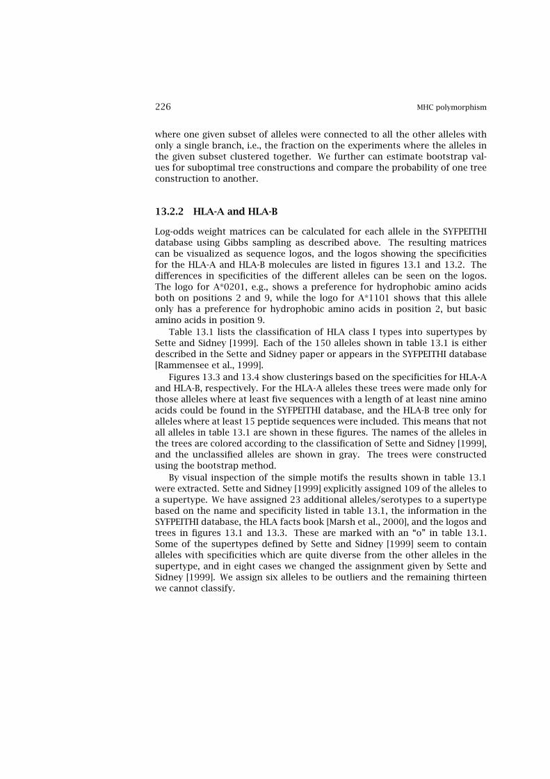
226 MHC polymorphism
where one given subset of alleles were connected to all the other alleles withonly a single branch, i.e., the fraction on the experiments where the alleles inthe given subset clustered together. We further can estimate bootstrap val-ues for suboptimal tree constructions and compare the probability of one treeconstruction to another.
13.2.2 HLA-A and HLA-B
Log-odds weight matrices can be calculated for each allele in the SYFPEITHIdatabase using Gibbs sampling as described above. The resulting matricescan be visualized as sequence logos, and the logos showing the specificitiesfor the HLA-A and HLA-B molecules are listed in figures 13.1 and 13.2. Thedifferences in specificities of the different alleles can be seen on the logos.The logo for A*0201, e.g., shows a preference for hydrophobic amino acidsboth on positions 2 and 9, while the logo for A*1101 shows that this alleleonly has a preference for hydrophobic amino acids in position 2, but basicamino acids in position 9.
Table 13.1 lists the classification of HLA class I types into supertypes bySette and Sidney [1999]. Each of the 150 alleles shown in table 13.1 is eitherdescribed in the Sette and Sidney paper or appears in the SYFPEITHI database[Rammensee et al., 1999].
Figures 13.3 and 13.4 show clusterings based on the specificities for HLA-Aand HLA-B, respectively. For the HLA-A alleles these trees were made only forthose alleles where at least five sequences with a length of at least nine aminoacids could be found in the SYFPEITHI database, and the HLA-B tree only foralleles where at least 15 peptide sequences were included. This means that notall alleles in table 13.1 are shown in these figures. The names of the alleles inthe trees are colored according to the classification of Sette and Sidney [1999],and the unclassified alleles are shown in gray. The trees were constructedusing the bootstrap method.
By visual inspection of the simple motifs the results shown in table 13.1were extracted. Sette and Sidney [1999] explicitly assigned 109 of the alleles toa supertype. We have assigned 23 additional alleles/serotypes to a supertypebased on the name and specificity listed in table 13.1, the information in theSYFPEITHI database, the HLA facts book [Marsh et al., 2000], and the logos andtrees in figures 13.1 and 13.3. These are marked with an “o” in table 13.1.Some of the supertypes defined by Sette and Sidney [1999] seem to containalleles with specificities which are quite diverse from the other alleles in thesupertype, and in eight cases we changed the assignment given by Sette andSidney [1999]. We assign six alleles to be outliers and the remaining thirteenwe cannot classify.
MHC Supertypes 227
Figure 13.1: Logos displaying the binding motifs for HLA-A molecules. The height of eachcolumn of letters is equal to the information content (in bits) at the given positions in thebinding motif. The relative height of each letter within each column is proportional to thefrequency of the corresponding amino acid at that position. Figure reprinted from Lund et al.[2004]. See plate 22 for color version.

228 MHC polymorphism

MHC Supertypes 229
Figure 13.2: Logos displaying the binding motifs for HLA-B molecules. For details on the logorepresentation, see figure 13.1. Figure reprinted from Lund et al. [2004]. See plates 23 and 24for color versions.

230 MHC polymorphismHLA-A1 A1 .[TS][DE].....Y HLA-A*0101a A1t .[–]......[–]HLA-A*0102a A1 .[–]......[–] HLA-A*0201 A2 .[LM]......[VL]HLA-A*0202 A2 .[AL]......[VL] HLA-A*0203 A2 .[LV]......[LI]HLA-A*0204 A2 .[AL]......[VL] HLA-A*0205 A2 .[LV]......[LS]HLA-A*0206 A2 .[VQ]......[VS] HLA-A*0207 A2 .[L-]......[VL]HLA-A*0209 A2o .[LA]......[V-] HLA-A*0214 A2o .[QV]......[LV]HLA-A*0217 A2o .[L-]......[L-] HLA-A3 A3 K[LY]......[KY]HLA-A*0301 A3 K[IL]......[K-] HLA-A*1101 A3 .[YT]......[K-]HLA-A23 . .[–]......[–] HLA-A*2301a A24 .[–]......[–]HLA-A24 A24t .[YF]......[LF] HLA-A*2402 A24 .[YF]......[LF]HLA-A*2403a A24t .[–]......[–] HLA-A*2404a A24t .[–]......[–]HLA-A25 A1t .[–]......[–] HLA-A*2501a A1t .[–]......[–]HLA-A26 A1t→A26 .[–]......[–] HLA-A*2601 A1t→A26 E[TI]......[FY]HLA-A*2602 A1t→A26 [DE]I......[FY] HLA-A*2603 A26o E[VL]......[ML]HLA-A*2604a A1t→A26 .[–]......[–] HLA-A28 A1→A26 .[–]......[–]HLA-A29 outlier .[FN]......[YC] HLA-A*2902 outlier K[E-]......[YL]HLA-A30a A24t .[–]......[–] HLA-A*3001 A24→A1 K[TF]......[FL]HLA-A*3002 A24t→A1 R[YV]......[YK] HLA-A*3003 A24t→A1 R[YL]......[Y-]HLA-A*3004 A1o K[YT]......[YL] HLA-A31 . .[–]......[–]HLA-A*3101 A3 [RK]QL.....[R-] HLA-A32 . .[–]......[–]HLA-A*3201a A1t .[–]......[–] HLA-A*3301 A3 .[LV]......[RK]HLA-A*3303 A3o [DE]I......[R-] HLA-A*3402 A3o .[V-]......[R-]HLA-A*3601a A1 .[–]......[–] HLA-A*4301a A1 .[–]......[–]HLA-A*6601 A3o [ED]T......[R-] HLA-A*6801 A3 E[VT]......[RK]HLA-A*6802 A2 D[TV]......[VS] HLA-A*6901 A2 E[TA]......[R-]HLA-A*7401 . .[T-]......[V-] HLA-A*8001a A1 .[–]......[–]HLA-B07X B7 .[PV]......[LA] HLA-B*0702 B7 .[PV]......[LA]HLA-B*0703 B7 .[DP]......[L-] HLA-B*0704a B7 .[–]......[–]HLA-B*0705 B7 .[P-]......[FL] HLA-B08 outlier .[LP]K.K...[L-]HLA-B*0801 outlier .[RK].[RK].... HLA-B*0802 outlier .[L-]K.K...[F-]HLA-B13 . .[A-]......[–] HLA-B*1301a B62t .[–]......[–]HLA-B*1302a B62t .[–]......[–] HLA-B14 outlier .[R-]......[LV]HLA-B*1401a B27 .[–]......[–] HLA-B*1402a B27 .[–]......[–]HLA-B39 B62o .[FM]......[YF] HLA-B*1501 B62 .[QL]......[YV]HLA-B*1502 B62 .[LQ]......[YF] HLA-B*1503 B27t .[QK]......[YV]HLA-B*1508 B7 .[PV]......[YS] HLA-B*1506a B62t .[–]......[–]HLA-B*1509 B27→B39 .[H-]......[LF] HLA-B*1510 B27t→B39 .[H-]......[LF]HLA-B*1512 B62t .[QL]......[YS] HLA-B*1513 B62 .[IL]......[W-]HLA-B*1514a B62t .[–]......[–] HLA-B*1516 B58 .[TS]......[IV]HLA-B*1517 B58 .[–]......[–] HLA-B*1518 B27t .[–]......[–]HLA-B*1519a B62t .[–]......[–] HLA-B*1521a B62t .[–]......[–]HLA-B17 . .[–]......[–] HLA-B18 B44h .[E-]......[–]HLA-B*1801 . .[–]......[–] HLA-B22 . .[–]......[–]HLA-B27 B27o .[R-]......[–] HLA-B*2701 B27t R[RQ]......[Y-]HLA-B*2702 B27 K[R-]......[YF] HLA-B*2703 B27 [RK]R......[LY]HLA-B*2704 B27 R[R-]......[LF] HLA-B*2705 B27 R[R-]F.....[–]HLA-B*2706 B27 R[R-]......[LV] HLA-B*2707 B27 [RK]R......[LV]HLA-B*2708a B27t .[–]......[–] HLA-B*2709 B27o [GR]R......[–]HLA-B35 B7o .[P-]......[Y-] HLA-B*3501X B7 .[PV]......[LY]HLA-B*3502a B7 .[–]......[–] HLA-B*3503 B7 .[PM]......[MF]HLA-B37 . .[F-]......[T-] HLA-B*3701 B44 .[DE].....L[I-]HLA-B*3801 B27→B39 .[HF]D.....[LF] HLA-B*3802a B27 .[–]......[–]HLA-B39 B27o .[H-]......[L-] HLA-B*3901 B27→B39 .[HR]......[L-]HLA-B*3902 B27 .[–]......[MF] HLA-B*3903a B27 .[–]......[–]HLA-B*3904a B27 .[–]......[–] HLA-B*3905 . .[–]......[–]HLA-B*3909 B27o→B39 .[RH]......[L-] HLA-B40 B44o E[F-]......[L-]HLA-B*4001 B44 .[E-]......[L-] HLA-B*4002 B44o .[E-]......[L-]HLA-B*4006 B44 .[E-]......[VA] HLA-B*4101a B44h .[–]......[–]HLA-B42 . .[PL]......[–] HLA-B44 B44 .[E-]......[–]HLA-B*4402 B44 .[E-]......[FL] HLA-B*4403 B44 E[E-]......[FW]HLA-B*4405 B44o .[E-]......[R-] HLA-B45 . .[–]......[–]HLA-B*4501 B44h .[E-]......[L-] HLA-B*4601 B62 .[MI]......[YF]HLA-B*4801 B27t .[QK]......[L-] HLA-B*4802a B27t .[–]......[–]HLA-B*4901a B44h .[–]......[–] HLA-B*5001a B44h .[QK]......[-L]HLA-B51 B7 .[AP]......[IL] HLA-B*5101 B7 .[AP]......[LY]HLA-B*5102 B7o .[PA]......[IV] HLA-B*5103 . .[FG]......[YI]HLA-B52a B62 .[–]......[–] HLA-B*5201 B62o .[QF]......[VF]HLA-B53 B7o .[P-]......[W-] HLA-B*5301 B7 .[P-]......[FL]HLA-B*5401 B7 .[P-]......[A-] HLA-B*5501 B7 .[P-]......[A-]HLA-B*5502 B7 .[P-]......[AV] HLA-B*5601 B7 .[P-]......[AL]HLA-B*5602a B7 .[–]......[–] HLA-B57 B58 .[AS]......[WT]HLA-B*5701 B58 .[ST]......[WF] HLA-B*5702 B58 .[TS]......[WF]HLA-B58 B58 .[–]......[–] HLA-B*5801 B58o .[TS]......[WF]HLA-B*5802 B58o .[ST]......[FM] HLA-B*6701 B7 .[P-]......[L-]HLA-B*7301 B27 .[R-]......[P-] HLA-B*7801 B7 .[GP]......[S-]
Table 13.1: HLA type (column 1,4), supertype (column 2,5) and amino acid motif (column 3,6)for all alleles described by Sette and Sidney [1999] and Rammensee et al. [1999]. Letters insquare parenthesis correspond to the same position. X: X-ray structure exists. Table adoptedfrom Lund et al. [2004]. a: Allele is not in SYFPEITHI. h/t: hypothetical/tentative supertypeassignment according to Sette and Sidney [1999]. o: the supertype assignment presented here.→: assignment changed by Lund et al. [2004].

MHC Supertypes 231
Figure 13.3: Tree showing clustering of HLA-A specificities. The alleles are colored accordingto the supertype classification by Sette and Sidney [1999]: A1: red, A2: orange, A3: black, A24:green, A29 and nonclassified alleles: gray. Figure reprinted from Lund et al. [2004]. See plate 25for color version.
13.2.3 HLA-A Supertypes
The tree describing the HLA-A alleles is characterized by five clusters: A1, A2,A3, A24, and A26. The corresponding branch bootstrap values are 0.37, 0.39,0.59, 0.98, and 0.38, respectively.
A2 supertype — hydrophobic amino acids in position 9: The resulting defini-tion of this supertype largely overlaps with the definition by Sette and Sidney[1999]. The unassigned HLA-A*0214 and HLA-A*0217 is added to the A2 su-pertype.
A3 supertype — basic amino acids in position 9: A*3303 and A*6601 areassigned to the A3 supertype characterized by basic amino acids in position 9.The other alleles in the cluster follow the classification suggested by Sette andSidney [1999].
A1 supertype — acidic amino acids in position 3: Here the clustering showsa large difference from the A1 supertype defined by Sette and Sidney [1999].The clustering suggests splitting the A1 supertype into two clusters. One clus-ter is the A1 cluster that contains the A1 and A*3001-4 alleles based on theircommon preference for acidic amino acids in position 3, and Y or F at posi-

232 MHC polymorphism
Figure 13.4: Tree showing clustering of HLA-B specificities. The alleles are colored according tothe supertype classification by Sette and Sidney [1999]: B7: black, B27: orange, B44: green, B58:blue, B62: violet, and nonclassified alleles and outliers (B8 and B46): gray. Figure reprinted fromLund et al. [2004]. See plate 26 for color version.
tion 9. The other cluster is a proposed new A26 supertype. Sette and Sidneyhave assigned HLA-A*3001-3 tentatively to an A24 supertype together with thealleles of A*24 and A*2402. The bootstrap branch value for the A24 clustersuggested by Sette and Sidney (A24, A*2402, A*3001, A*3002, and A*3003)is found to be 0.02. Also the bootstrap value for a cluster containing boththe A2601, A*2602, and the A1 alleles is below 0.01. These numbers stand incontrast to the bootstrap branch values for the A1 cluster and the new A26clusters, which are 0.37 and 0.38, respectively.
Proposed new A26 supertype — acidic amino acids in position 1: HLA-A*2601-3 have E/D in position 1 rather than at position 3 in HLA-A1. Thisdifference is consistent with the motif descriptions by Marsh et al. [2000].These alleles therefore form a new supertype. Including HLA-A*2902 in theA26 supertype leads to a decrease in the branch bootstrap value from 0.38 to0.12, so this allele is left as an outlier.

MHC Supertypes 233
A24-supertype — tyrosine or hydrophobic in position 2: A24 and A*2402 isassigned to the A24 supertype. These alleles have a bootstrap value of 0.98.
Based on the background of what is described above, a redefinition of theA1 supertype is made: The HLA-A*2601/2 alleles may form a new separate A26supertype. The following alleles remain unclassified: A23, A31, A32, A*7401.
13.2.4 HLA-B Supertypes
The HLA-B supertype tree contains many more alleles than the HLA-A tree.In order to make the clustering analysis more feasible and clear, the HLA-B clustering is limited to the alleles where at least 15 peptide sequences areavailable in either the SYFPEITHI or MHCPEP databases. This limits the analysisto 45 HLA-B alleles out of 99 available.
B7 supertype — proline in position 2: The definition of the B7 supertype bySette and Sidney [1999] largely corresponds to the B7 cluster in figure 13.4, butwith one important exception. Sette and Sidney place the HLA-B*1508 in theB7 supertype. However, the bootstrap branch value for the Sette and Sidney B7cluster is 0.042, whereas the corresponding value for the B7 cluster, excludingthe HLA-B*1508 allele, is 0.66.
New B8 supertype — lysine in position 3 and 5: The B8 alleles were definedas an outlier group by Sette and Sidney [1999] and the specificities of B*08,and B*0802 define a cluster with a corresponding branch bootstrap value of0.72 in figure 13.4.
B62 supertype — tyrosine in position 9: The B62 cluster shown in figure13.4 is restricted to contain only the alleles HLA-B*1503, HLA-B*1501, HLA-B*1502, and HLA-B*1508. The bootstrap branch value for the cluster is 0.62.Including the alleles HLA-B*1516 and HLA-B*5201 make the bootstrap valuedrop to 0.06. These two alleles are thus left out as outliers. The bootstrapbranch value for the B62 cluster defined by Sette and Sidney is < 10-3. This lowbranch value is due to the misplacement of the HLA-B*1513 and HLA-B*5201alleles in the B62 supertype, and the HLA-B*1508 allele in the B7 supertype.
B27 supertype — basic in position 2: The definition of the B27 supertypeby Sette and Sidney has a branch bootstrap value < 10-3, whereas the B27cluster defined in figure 13.4 has a branch value of 0.22. The low branchvalue for the Sette and Sidney B27 supertype is due to a misplacement of theHLA-B*1503 allele. As described above, this allele is placed in the B62 cluster.Splitting up the B27 cluster into two subclusters leaving out the HLA-B*7301and the HLA-B*14 alleles as outliers, leads to a bootstrap branch value for theremaining B27 cluster of 0.62. The other alleles form a new B39 supertype witha bootstrap branch value of 0.41. The B39 cluster contains the alleles of HLA-B3909, HLA-B*3901, HLA-B*3801, HLA-B*1510, and HLA-B*1509. These alleles

234 MHC polymorphism
have similar B and F pocket residues as defined by Sette and Sidney [1999].The redefined B27 cluster contains the alleles of HLA-B*2705, HLA-B*2703,HLA-B*2704, HLA-B*2706, HLA-B27, HLA-B*2701, and HLA-B*2702.
B44 supertype — glutamic acid in position 2: The definition of the B44 clus-ter largely corresponds to the supertype definition of Sette and Sidney [1999].The alleles of HLA-B*40 and HLA-B*44 are included in the supertype, and thebootstrap branch value for the cluster is then 0.36.
B58 supertype — hydrophobic at position 9: The branch bootstrap value forthe B58 cluster defined in figure 13.4 is found to be 0.42. Including the HLA-B*1517 allele this value drops to 0.18, thus this allele is left out as an outlier.The bootstrap value for the Sette and Sidney [1999] B58 supertype is 0.156.Leaving out the HLA-B*1516 and HLA-B*1517 alleles as outliers as describedabove and including the HLA-B*1513 allele lead to the B58 cluster defined infigure 13.4.
There is generally good consistency between the supertypes defined bySette and Sidney [1999] and the HLA-B tree. In addition, B8 is a novel su-pertype including the HLA-B*08 and HLA-B0802 alleles as well as splitting theB27 supertype into two, a B39 supertype and a B27 supertype. Further, someof the alleles could be rearranged so as to increase the likelihood of the clus-tering. The following HLA-B alleles remain unclassified: B17, B*1801, B22, B37,B*3905, B42, B45 (two sequences in SYFPEITHI, both with E in position 2), andB*5301. Only one or two sequences were found in SYFPEITHI for these alleles,except for B17, where five sequences were found.
13.2.5 Do Cross-Loci Supertypes Exist?
The alleles within the supertypes defined by Sette and Sidney [1999] are allencoded by either the A or the B locus. Making a tree of all the HLA-A and HLA-B alleles included in the analysis described above, no mixing of the HLA-A andHLA-B clusters is found. Only the outliers HLA-B*1516 and HLA-A*2902 mixwith a cluster defined by the opposite locus. The HLA-B*1516 allele clusterswithin the A1 supertype consistent with a preference for T and S at position2, and a preference for Y, F, L, and V at position 9. The HLA-A2902 alleleclusters within the B44 supertype consistent with a preference for E at position2 and a preference for Y in position 9 found in both motifs. The A*2902molecule used for elution of peptides is often purified from the Ebstein-Barrvirus-transformed cell line SWEIG which coexpresses B*4402, and the apparentsimilarity may be an experimental artifact caused by cross-reactivity of theantibody used for purification from this cell line. This unrelatedness of HLA-Aand HLA-B molecules may be a direct result of evolutionary pressure on theimmune system to provide optimal protection against infectious diseases. To
MHC Supertypes 235
obtain optimal peptide coverage, it is beneficial for the immune system to havea highly diverse set of HLA specificities. A simple way to achieve this could beto have the HLA-A and HLA-B alleles evolve in an orthogonal manner.
13.2.6 HLA-DR
For most class II molecules relatively few binding peptides are known. Tocompensate for that the similarities between different alleles are calcu-lated, based on other published specificity matrices. Specificity matrices forHLA class II molecules can be downloaded from, e.g., the ProPred website(http://www.imtech.res.in/raghava/propred/page4.html). The list of alleles isgiven in table 13.2. These matrices were constructed by Singh and Raghava[2001] using the TEPITOPE (http://www.vaccinome.com) method [Hammeret al., 1994, Sturniolo et al., 1999].
To test whether the matrices in the ProPred server are similar to those inthe TEPITOPE program, test sequences can be submitted to both programs aswell as to a program using the matrices from ProPred. The matrix scores areused to estimate the amino acid frequencies at different positions in the motif,assuming that the matrix score is proportional to a log-odds score. The oddsscore is defined as the probability of observing amino acid a in position p ina binding peptide relative to the probability of observing that amino acid inproteins in general. Thus,
ppa =exp(spa)qa∑i exp(spi)qi
, (13.2)
where spa is the matrix score of amino acid a on position p, and qa is thebackground frequency of the amino acid.
Sequence logos were constructed to visualize the specificities. By visual in-spection of different HLA class II molecules (figure 13.5) it is clear that someof these are quite similar. In order to quantify the similarities, the distancebetween all pairs of matrices was calculated. These distances were then usedto construct a tree visualizing the similarities between the peptides that eachallele binds (figure 13.6). Based on this tree, the HLA-DR molecules are di-vided into nine clusters or supertypes. The clusters may be represented byDRB1*0101 (1, 0.92), DRB1*0301 (3, 0.65), DRB1*0401 (4, 0.45), DRB1*0701(7, 1.0), DRB1*0813 (8, 0.52), DRB1*1101 (11, 0.32), DRB1*1301 (13, 0.39),DRB1*1501 (15, 0.82), and DRB5*0101 (51, 0.95). Here the numbers in paren-theses after each allele name correspond to the supertype name assigned toeach cluster in figure 13.5, and the cluster bootstrap branch value, respec-tively. The alleles in figure 13.5 are colored according to the serotype.

236 MHC polymorphism
Allele Sero type Pocket profile SupertypeHLA-DRB1*0101 DR1 [1;1;1;1;1] 1HLA-DRB1*0102 DR1 [2;1;1;1;1] 1HLA-DRB1*0301 DR3 [2;3;3;3;2] 3HLA-DRB1*0305 DR3 [1;3;3;3;3] 3HLA-DRB1*0306 DR3 [2;3;3;4;3] 3HLA-DRB1*0307 DR3 [2;3;3;4;3] 3HLA-DRB1*0308 DR3 [2;3;3;4;3] 3HLA-DRB1*0309 DR3 [1;3;3;3;2] 3HLA-DRB1*0311 DR3 [2;3;3;4;3] 3HLA-DRB1*0401 DR4 [1;4;4;4;3] 4HLA-DRB1*0402 DR4 [2;5;4;5;3] 4HLA-DRB1*0404 DR4 [2;6;4;6;3] 4HLA-DRB1*0405 DR4 [1;6;4;6;5] 4HLA-DRB1*0408 DR4 [1;6;4;6;3] 4HLA-DRB1*0410 DR4 [2;6;4;6;5] 4HLA-DRB1*0421 DR4 [1;4;4;4;2] 4HLA-DRB1*0423 DR4 [2;6;4;6;3] 4HLA-DRB1*0426 DR4 [1;4;4;4;3] 4HLA-DRB1*0701 DR7 [1;8;5;8;4] 7HLA-DRB1*0703 DR7 [1;8;5;8;4] 7HLA-DRB1*0801 DR8 [1;9;3;9;5] 8HLA-DRB1*0802 DR8 [1;9;3;9;3] 8HLA-DRB1*0804 DR8 [2;9;3;9;3] 8HLA-DRB1*0806 DR8 [2;9;3;9;5] 8HLA-DRB1*0813 DR8 [1;9;3;6;3] 8HLA-DRB1*0817 DR8 [1;9;3;7;5] 8HLA-DRB1*1101 DR11 [1;7;3;7;3] 11HLA-DRB1*1102 DR11 [2;11;3;11;3] 13HLA-DRB1*1104 DR11 [2;7;3;7;3] 11HLA-DRB1*1106 DR11 [2;7;3;7;3] 11HLA-DRB1*1107 DR11 [2;3;3;3;3] 3HLA-DRB1*1114 DR11 [1;11;3;11;3] 13HLA-DRB1*1120 DR11 [1;11;3;11;2] 13HLA-DRB1*1121 DR11 [2;11;3;11;3] 13HLA-DRB1*1128 DR11 [1;7;3;7;2] 11HLA-DRB1*1301 DR13 [2;11;3;11;2] 13HLA-DRB1*1302 DR13 [1;11;3;11;2] 13HLA-DRB1*1304 DR13 [2;11;3;11;5] 13HLA-DRB1*1305 DR13 [1;7;3;7;2] 11HLA-DRB1*1307 DR13 [1;7;3;9;3] 11HLA-DRB1*1311 DR13 [2;7;3;7;3] 11HLA-DRB1*1321 DR13 [1;7;3;7;5] 11HLA-DRB1*1322 DR13 [2;11;3;11;3] 13HLA-DRB1*1323 DR13 [1;11;3;11;3] 13HLA-DRB1*1327 DR13 [2;11;3;11;2] 13HLA-DRB1*1328 DR13 [2;11;3;11;2] 13HLA-DRB1*1501 DR2 [2;2;2;2;1] 15HLA-DRB1*1502 DR2 [1;2;2;2;1] 15HLA-DRB1*1506 DR2 [2;2;2;2;1] 15HLA-DRB5*0101 DR2 [1;10;6;10;6] 51HLA-DRB5*0105 DR2 [1;10;6;10;6] 51
Table 13.2: A list of the HLA class II alleles used. The list contains the allele, serotype(Type), pocket profile, and our supertype assignment. The pocket profiles used in as-sembly of virtual DR matrices are from Sturniolo et al. [1999]. For each allele the listof numbers in square parenthesis denotes which pocket specificity has been used to con-struct the profile for position 1, 4, 6, 7, and 9 (positions 2 and 3 were derived from theDRB1*0401 matrix). The matrix for HLA-DRB1*0421 could not be found at the ProPred web-site (http://www.imtech.res.in/raghava/propred/page4.html) when the work was done. Tableadopted from Lund et al. [2004].

MHC Supertypes 237
The clustering roughly corresponds to the serotype classification, but withsome important exceptions. Note, e.g., the mixing of the DR11, and DR13 se-quences and that DRB1*1107 clusters with the DR3 sequences. The bootstrapvalue for the DR11 and DR13 serotype clusters are, e.g., < 0.001 and the boot-strap value for the DR3 serotype cluster, excluding the DRB1*1107 allele, is0.03. The matrices were constructed under the assumption that the aminoacids at different positions contribute independently (by binding to a pocketin the HLA molecule) to the binding of the peptide. Furthermore, it is alsoassumed that HLA molecules with the same amino acids in a given pocket willhave the same specificity profile [Hammer et al., 1997]. Different matrices thushave the same profile at a given position if the corresponding HLA moleculesshare the amino acids lining the pocket for that position. In table 13.2 it can beseen that DRB1*1107 and DRB1*0305 only differ in one binding pocket. Thisis hence consistent with placing the DRB1*1107 allele in the DR3 supertype.Similarly, it seems that the alleles placed in the DR11 and DR13 supertypes inmost cases share three out of the five pocket specificities.
13.2.7 Experimental Verification of Supertypes
To verify the clustering suggested above, weight matrices for all the class Ialleles in this study were constructed as earlier described. These weight matri-ces can then be used to predict the binding affinity for sets of peptides, wherethe binding affinity to a specific HLA allele had been measured experimen-tally. Alleles for which experimental binding information is available are, e.g.,HLA-A*0101 (A1), HLA-A0202 (A2), HLA-A*0301 (A3), HLA-A*1101 (A3), HLA-A*3101 (A3 outlier), HLA-B*2705 (B27), HLA-B*1501 (B62), HLA-B*5801 (B58),and HLA-B*0702 (B7) [Sylvester-Hvid et al., 2004]. Here the name written inparentheses refers to the supertype classification. The linear correlation co-efficient, also known as Pearson’s r [Press et al., 1992], is calculated betweenthe prediction score and the log of the measured binding affinity. It is nowexpected that alleles with similar specificity to that of the allele used in theexperiments will obtain a positive correlation, and that other alleles will get acorrelation close to zero. This calculation actually supports most of the resultsobtained from the clustering analysis [Lund et al., 2004].
One of the advantages with this kind of clustering is that it can easily berecalculated if new data become available in the future. The availability of datais expected to increase as the epitope immune database, and several large-scaleepitope discovery projects funded by the NIH have been started. Additionalmaterial is available at:http://www.cbs.dtu.dk/researchgroups/immunology/supertypes.htmland will be updated whenever new data become available.

238 MHC polymorphism
Figure 13.5: Logos displaying the binding motifs for 50 different HLA class II molecules. Fordetails of the logo representation, see figure 13.1. Figure reprinted from Lund et al. [2004]. Seeplate 27 for color version.

MHC Supertypes 239
Figure 13.6: Tree showing the clustering of 50 different HLA class II molecules based on theirpeptide-binding specificity. The proposed clusters are encircled and labeled. Figure reprintedfrom Lund et al. [2004]. See plate 28 for color version.
The clusters define groups of alleles with similar binding specificities. Inorder to get a broad coverage of the human population with an epitope-basedvaccine, it must be ensured that most people from all ethnic groups have anHLA molecule with specificity for at least one of the peptides in the vaccine.This can in turn be obtained making sure that the specificity defined by eachcluster is covered by one peptide in the vaccine.

Chapter 14
Predicting Immunogenicity: AnIntegrative Approach
The genome era provides opportunities to study the immune system froma systems biology perspective as discussed in chapter 1. We now have notonly the sequence information that sheds light on the immunological diversityamong individuals in a population but also advanced techniques that allowus to obtain a better estimate of the kinetics and specificity of an immuneresponse. In this chapter we will give an example of such systems biologyapproaches to immunology: prediction of immunogenic regions for cytotoxicT cells. A very similar study is published by Larsen et al. [2005].
Reliable prediction of immunogenic peptides may be useful for many ap-plications, e.g., for rational vaccine design. Many attempts have been made topredict the outcome of the steps involved in antigen presentation. As we havedescribed earlier in the book, a number of methods have been developed thatvery reliably predict the binding affinity of peptides to the different MHC-I al-leles [Brusic et al., 1994, Buus et al., 2003, Nielsen et al., 2003, 2004]. Likewise,a method has been developed that predicts the efficiency by which peptides ofarbitrary length can be transported by TAP [Peters et al., 2003a]. Several meth-ods have also been developed that aim at predicting the proteasomal cleavagepattern of proteins (see chapter 7 for details).
Can predictions of proteasomal cleavage patterns and TAP transport effi-ciency contribute to an improved identification of epitopes compared to thatobtained when using only predictions of MHC-I affinity? Peters et al. [2003a]have shown that combining MHC-I affinity predictions with prediction of TAPtransport efficiency leads to improved identification of CTL epitopes. Thisanalysis can be extended to address, for a large set of different HLA alleles,
241

242 Predicting immunogenicity: An integrative approach
if a combined prediction method mimicking the MHC I pathway can improveprediction of epitopes. The following analysis includes epitopes from close to70 different MHC alleles from different MHC-I supertypes [Sette and Sidney,1999, Lund et al., 2004]. The proteasomal cleavage event were modeled byprediction algorithms as described in chapter 7.
To validate the integrative method, a data set (SYF) containing 152 9merepitopes restricted to more than 70 different HLA alleles extracted from theSYFPEITHI database (http://syfpeithi.bmi-heidelberg.com/) are uesd. The ma-jority of these peptides have successfully passed the steps involved in anti-gen presentation. The set of negative peptides (peptides that will not bepresented by the MHC class I pathway) were defined as all 9mer peptidescontained in the protein sequences from which the epitopes originated, ex-cept those annotated as epitopes in either the complete SYFPEITHI or LosAlamos HIV databases (www.hiv.lanl.gov/immunology. When using this def-inition of epitopes/nonepitopes one has to take into account that some 9merswill falsely be classified as nonepitopes because the SYFPEITHI and Los AlamosHIV databases are incomplete. Since the HLA molecules have a very specificpeptide binding repertoire, this false-negative proportion will be very small. Ina protein of 200 amino acids, one expects to have one binding, and approxi-mately 199 nonbinding peptides [Yewdell and Bennink, 1999]. The potentialnumber of false negatives is hence orders of magnitude smaller than the actualnumber of negatives.
14.1 Combination of MHC and Proteasome Predictions
To examine whether predictions of proteasomal cleavage can contribute to theclassification of peptides into epitopes/nonepitopes independently of the pre-dicted MHC-I binding affinity, one option is to perform a sort/split experiment:two groups of peptides with approximately equal predicted MHC-I affinity, butdifferent predicted proteasomal cleavage, is generated. All 9mer peptides ineach protein is individually sorted according to their predicted MHC-I affinity.Looking at two peptides at a time from the top of the sorted list, they arethen split into two groups and the peptide with highest predicted proteasomalcleavage value is put in group H, whereas the peptide with the lowest is putin group L. Figure 14.1 shows, for four different methods predicting proteaso-mal cleavage, how the number of epitopes in the H group deviates from theexpected number (50%).
To test if the number of epitopes is significantly different in group H ascompared to group L, the binomial distribution is applied. Under the nullhypothesis, the epitopes have an equal chance of falling into either group,π0 = 0.5. If n is the total number of epitopes, the expected number of epitopes

Independent Contributions from TAP and Proteasome Predictions 243
in either group is π0 n. If r is the observed number of epitopes in one of thegroups, the departure from the expected number can be expressed by the z-score [Armitage et al., 2004]:
z = r −nπ0√nπ(1−π)
. (14.1)
The nullhypothesis is rejected at p = .05 if z > 1.96, at p = .01 if z > 2.58,and at p = .001 if z > 3.29.
All four proteasomal cleavage methods the number of epitopes is signifi-cantly higher in group H than in group L. The method with the poorest perfor-mance is that of NetChop 20S with a p-value just below .01. The other threemethods all separate the H from the L group with p-values below or close to.001. For NetChop 2.0, for example, 34% or 72% more epitopes are found in theH group. Figure 14.1 also shows that the predicted cleavage patterns of theinternal amino acids add very little extra information to the predicted MHC-Iaffinity. When using NetChop 2.0 or NetChop 3.0 to study the predicted cleav-age at position 1, only 38% and 39%, respectively, of the epitopes are locatedin group H. This may indicate that peptides with a high predicted proteasomalcleavage value at this position are rarely epitopes. If, however, the NetChop20S or NetChop 20S-3.0 network is used, this scenario is reversed.
Applying the bootstrap [Press et al., 1992] method you find that theNetChop 20S method performs significantly worse than the other methods(p < .05 in all three comparisons). The difference in predictive performancebetween the other methods is, however, statistically insignificant (p > .05 inall cases). Thus, this analysis demonstrates that only the methods based on invivo cleavage data can improve the identification of epitopes in combinationwith the predicted MHC-I affinity.
14.2 Independent Contributions from TAP and Proteasome Pre-dictions
To address the question of whether proteasomal cleavage and TAP trans-port efficiency can contribute independently to the identification of epitopes asort/split experiment sorting on TAP transport efficiency and splitting on pro-teasomal cleavage was conducted. When examining if cleavage predictions cancontribute to the identification of epitopes independently of the predicted TAPtransport efficiency, two groups of peptides with close to equal TAP transportefficiency, but different predicted proteasomal cleavage, were generated us-ing the same method as described in the previous section. In this experimentthe two groups H and L thus have similar TAP transport efficiency, but verydifferent predicted proteasomal cleavage values. The result of the analysis is

244 Predicting immunogenicity: An integrative approach
Figure 14.1: Sort/split experiment conducted sorting on predicted MHC-I affinity, splitting onpredicted proteasomal cleavage. Two groups with close to equal MHC-I affinity, but with differ-ent predicted proteasomal cleavage. In total, the two groups contain 152 epitopes. The figureshows the number of epitopes in group H deviating from the expected number of 76 (50%) L. 1-9:position 1-9 of the peptide (9 is the C-terminal end). Four different methods have been used forpredicting proteasomal cleavage: NetChop 20S, NetChop 20S-3.0, NetChop2.0, and NetChop3.0.Also shown are lines indicating levels of significance estimated as described in the text.
shown in figure 14.2, where NetChop 3.0 has been used for the proteasomalcleavage predictions. The figure shows how the number of epitopes in theH group deviates from the expected number (50%). In combination with TAPtransport efficiency only, the predicted C-terminal cleavage can contribute sig-nificantly to the identification of the epitopes. There is an excess number of30 epitopes between the H and L groups, corresponding to 70%. This resultdemonstrates that not all TAP transported peptides are cleaved equally wellby the proteasome. Between two groups of peptides with equal TAP transportefficiencies, epitopes are found predominantly in the group with high protea-somal C-terminal cleavage.
Next a sort/split experiment sorting on MHC-I affinity and splitting on TAPtransport efficiency is conducted to investigate if TAP transport efficiency andMHC-I binding can contribute independently to the identification of epitopes.In the experiment, most epitopes (66%, p < .001) fall into the group with highTAP transport efficiency. Among peptides with similar MHC-I affinity, peptideswith high TAP transport efficiency are thus most likely to be epitopes.
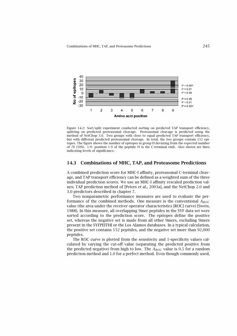
Combinations of MHC, TAP, and Proteasome Predictions 245
Figure 14.2: Sort/split experiment conducted sorting on predicted TAP transport efficiency,splitting on predicted proteasomal cleavage. Proteasomal cleavage is predicted using themethod of NetChop 3.0. Two groups with close to equal predicted TAP transport efficiency,but with different predicted proteasomal cleavage. In total, the two groups contain 152 epi-topes. The figure shows the number of epitopes in group H deviating from the expected numberof 76 (50%). 1-9: position 1-9 of the peptide (9 is the C-terminal end). Also shown are linesindicating levels of significance.
14.3 Combinations of MHC, TAP, and Proteasome Predictions
A combined prediction score for MHC-I affinity, proteasomal C-terminal cleav-age, and TAP transport efficiency can be defined as a weighted sum of the threeindividual prediction scores. We use an MHC-I affinity rescaled prediction val-ues; TAP prediction method of [Peters et al., 2003a], and the NetChop 2.0 and3.0 predictors described in chapter 7.
Two nonparametric performance measures are used to evaluate the per-formance of the combined methods. One measure is the conventional AROCvalue (the area under the receiver operator characteristics [ROC] curve) [Swets,1988]. In this measure, all overlapping 9mer peptides in the SYF data set weresorted according to the prediction score. The epitopes define the positiveset, whereas the negative set is made from all other 9mers, excluding 9merspresent in the SYFPEITHI or the Los Alamos databases. In a typical calculation,the positive set contains 152 peptides, and the negative set more than 92,000peptides.
The ROC curve is plotted from the sensitivity and 1-specificity values cal-culated by varying the cut-off value (separating the predicted positive fromthe predicted negative) from high to low. The AROC value is 0.5 for a randomprediction method and 1.0 for a perfect method. Even though commonly used,

246 Predicting immunogenicity: An integrative approach
the AROC measure is not easy to interpret intuitively. A second performancemeasure with a clear and intuitive interpretation is a rank measure: for eachprotein in the benchmark, all 9mer peptides are sorted based on the predic-tion score. A given protein may appear more than once in the benchmark if itcontains more than one epitope. The rank value for the protein is calculatedas the number of nonepitopes with a score higher than that of the correspond-ing epitope. From these rank values a rank curve showing the accumulativefraction of proteins with a rank value below a certain value was constructed.From the rank curve one can then extract information on how large a fractionof the proteins will have the epitope within a rank of, e.g., 25. Finally, a sin-gle performance measure (ARANK) as the area under the rank curve integratedfrom rank zero up to rank 100 was defined. A perfect prediction method willhave all the epitopes as rank 1, and thus an ARANK value of 1.0, whereas a poormethod will have the epitopes well below rank 100 and hence an ARANK valueof 0.0. Examples of a ROC and a rank curve are shown in figure 14.3. For boththe AROC and ARANK performance measures, one should be aware that some9mers will falsely be classified as nonepitopes because the SYFPEITHI and LosAlamos HIV databases are incomplete.
The SYF data set is used to estimate the set of weights where the ARANKand AROC values are optimal. Next the optimal combined prediction schemeis applied to an HIV data set of 69 epitopes derived from the Los Alamos HIVdatabase to estimate the performance gain on an independent evaluation dataset.
The optimal combined method is found to have relative weights onC-terminal cleavage and TAP transport efficiency of 0.15 and 0.115, respec-tively. In figure 14.3, we show examples of ROC and rank curves for theSYF data set. The figure shows the performance curves for five differentprediction scoring schemes: Comb, MHC, TAP, NetChop 2.0, and NetChop3.0. Here, the Comb method is the combined method with relative weight onTAP and NetChop 3.0 of 0.115 and 0.15, respectively, while others are singlepredictions. In figure 14.4, we give the details of the performance measuresfor the different methods and their combinations.
The curves shown in figure 14.3 clearly highlight the problematic aspectsof using the AROC performance measure when dealing with highly unbalanceddata sets. The AROC values for the NetChop 3.0 and TAP prediction methodsare close to identical (see figure 14.4). However, looking at the ROC curves foreach method, it is clear that the NetChop 3.0 method provides the most usefulpredictions. The region of the ROC curve where the TAP predictor performsbest falls in a highly nonrelevant region of the specificity. The two curves crossat a false-positive ratio of 0.4. This value corresponds to 40% false-positivepredictions, and having an improved prediction method only in this specificityrange is clearly irrelevant. For the rank curves this problem is not present, and

Combinations of MHC, TAP, and Proteasome Predictions 247
Figure 14.3: ROC and rank performance curves for different prediction methods. Left: the ROCcurves. Right: rank curves. ARANK is the area under the rank curve (highlighted as the shadedarea under the TAP curve) as described in the text. Predictions are made on the SYF data set.The different prediction methods are; Comb: optimal combined method with relative weight onC-terminal cleavage and TAP transport efficiency of 0.15 and 0.115, respectively; MHC: MHC-Iaffinity; TAP: TAP transport efficiency; NetChop 3.0: C-terminal cleavage by NetChop; NetChop2.0: C-terminal cleavage by NetChop 2.0. The inserts to the figures show high specificity/highrank, part of the corresponding curves.
we can directly identify the most relevant method from the integrated ARANKvalue.
The results shown in figures 14.3 and 14.4 demonstrate that the combinedmethod integrating prediction of proteasomal cleavage, TAP transport, andMHC affinity has the highest performance in terms of both the AROC andARANK values. The individual method with the poorest performance is that ofNetChop 20S, followed by NetChop 20S-3.0, TAP, the NetChop 2.0 and NetChop3.0 methods, and MHC-I affinity.
What is also clear from the results shown is that the combined methodhas a predictive performance superior to that of both MHC-I affinity aloneand any method integrating prediction of MHC-I affinity with TAP transportefficiency or C-terminal proteasomal cleavage. The performance values forMHC, MHC+TAP, MHC+NetChop 3.0, and the combined method are 0.88, 0.90,0.90, 0.91 for AROC and 0.70, 0.75, 0.73, 0.76 for ARANK respectively. Com-paring the performance values for the combined method to that of MHC-I,MHC-I+TAP, and MHC-I+NetChop 3.0, we find the following bootstrap hypoth-esis test values: <0.01, <0.01, <0.01 and 0.025, <0.01, <0.01 for AROC and
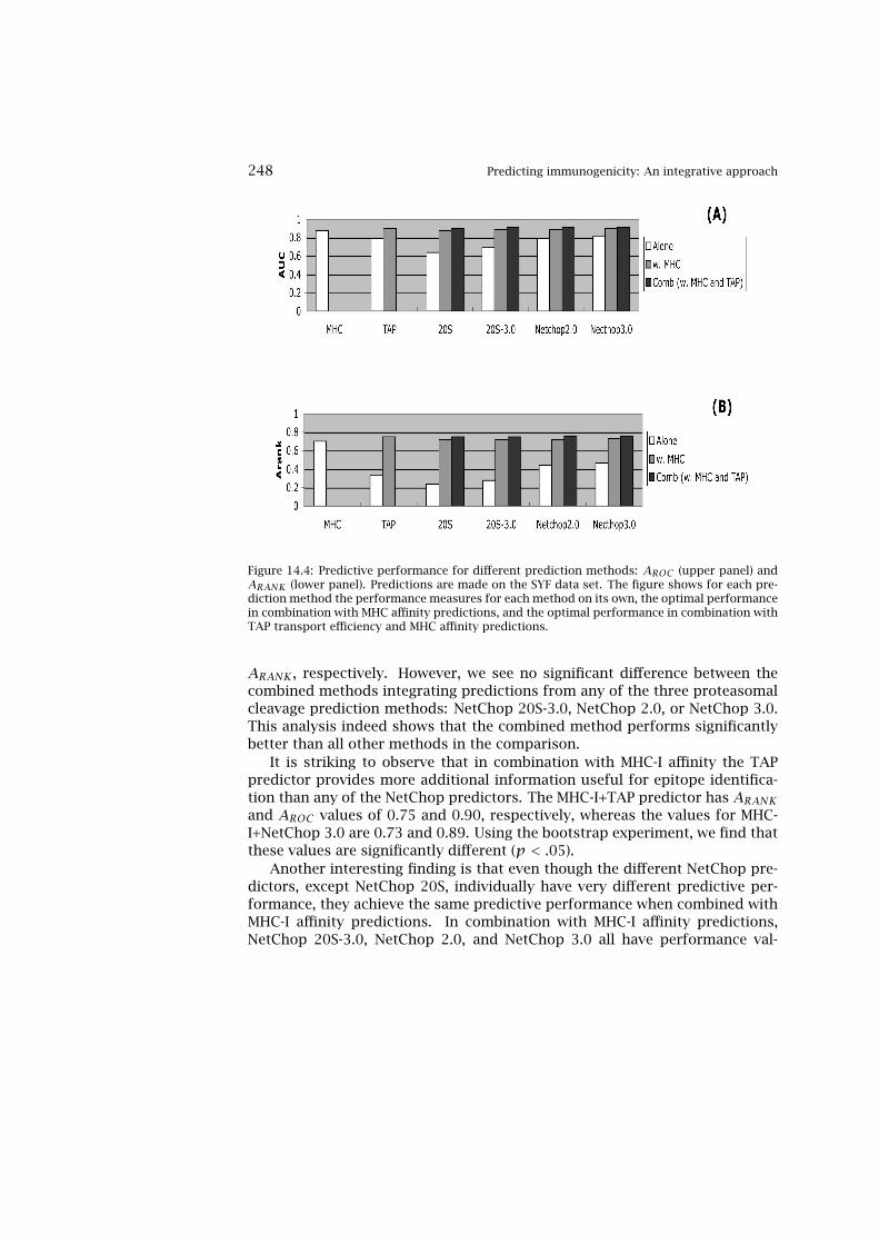
248 Predicting immunogenicity: An integrative approach
Figure 14.4: Predictive performance for different prediction methods: AROC (upper panel) andARANK (lower panel). Predictions are made on the SYF data set. The figure shows for each pre-diction method the performance measures for each method on its own, the optimal performancein combination with MHC affinity predictions, and the optimal performance in combination withTAP transport efficiency and MHC affinity predictions.
ARANK , respectively. However, we see no significant difference between thecombined methods integrating predictions from any of the three proteasomalcleavage prediction methods: NetChop 20S-3.0, NetChop 2.0, or NetChop 3.0.This analysis indeed shows that the combined method performs significantlybetter than all other methods in the comparison.
It is striking to observe that in combination with MHC-I affinity the TAPpredictor provides more additional information useful for epitope identifica-tion than any of the NetChop predictors. The MHC-I+TAP predictor has ARANKand AROC values of 0.75 and 0.90, respectively, whereas the values for MHC-I+NetChop 3.0 are 0.73 and 0.89. Using the bootstrap experiment, we find thatthese values are significantly different (p < .05).
Another interesting finding is that even though the different NetChop pre-dictors, except NetChop 20S, individually have very different predictive per-formance, they achieve the same predictive performance when combined withMHC-I affinity predictions. In combination with MHC-I affinity predictions,NetChop 20S-3.0, NetChop 2.0, and NetChop 3.0 all have performance val-

Validation on HIV Data Set 249
ues close to 0.90 and 0.73 for AROC and ARANK , respectively, and the indi-vidual performance differences are statistically significant. Finally, we alsofound that the NetChop 20S-3.0 and TAP predictors can be combined in a con-structive manner with a predictive performance significantly higher than thatof the individual predictors. This is, however, not the case for the NetChop3.0 predictor. Here the combination with TAP only leads to a minor and in-significant improvement in the predictive performance (data not shown). Thisanalysis suggests that the NetChop predictor trained on epitope data does in-deed predict a combination of MHC-I affinity, TAP transport efficiency, andproteasomal cleavage rather than just proteasomal cleavage. As an individ-ual prediction method for epitope recognition, the NetChop method trainedon epitope data clearly outperforms the methods trained on in vitro degra-dation data. However, when combined with MHC-I affinity and TAP transportefficiency predictions both the epitope and in vitro trained methods achievesimilar performance.
A direct measure of the performance gain when comparing the combinedmethod to that of MHC-I affinity prediction alone is the rank number needed inorder to identify 75% of the epitopes in the benchmark. For the MHC-I affinitypredictions alone this rank number is 55, meaning that in a set of proteinsone will have to test 55 peptides from each protein in order to identify 75% ofthe epitopes. For the combined method this number has dropped to 30. Eventhough this number is still high, the performance gain is clearly notable.
14.4 Validation on HIV Data Set
The above analysis can be done for indivual pathogens, like HIV. The resultsof such an analysis are shown in figure 14.5 and confirm the findings from theSYF data set. The combined method has a performance superior to that of allthe individual methods. The TAP transport predictor has the poorest perfor-mance, followed by that of NetChop 3.0. Estimating the rank number neededin order to identify 75% of the epitopes in the benchmark, we find values of52 and 30 for the MHC-I predictor alone and the combined method, respec-tively. These numbers thus confirm the values found when using the SYF dataset. A direct implication of this performance gain is a twofold reduction in theexperimental efforts needed to identify 75% of the epitopes in a large set ofproteins.

250 Predicting immunogenicity: An integrative approach
Figure 14.5: Performance for different prediction methods. Predictions are made on the HIV dataset. The figure shows the predictive performance for the three individual prediction methodsof MHC, C-terminal cleavage (NetChop 3.0), and TAP, as well as the combined method (Comb)with relative weight on C-terminal cleavage and TAP transport efficiency of 0.15 and 0.115,respectively.
14.5 Perspectives on Data Integration
In this chapter, we have demonstrated how an integrative approach combiningpredictions of the proteasomal cleavage, TAP transport efficiency, and MHC-Iaffinity can lead to improved CTL epitope recognition.
Other groups have previously combined different prediction methods: Hak-enberg et al. [2003] developed a bioinformatical tool for prediction of CTL epi-topes by combining prediction of proteasomal cleavage and MHC affinity. Ona very small data set of only five epitopes from HIV-1 Nef, Kesmir et al. [2002]showed that combining predictions of proteasomal cleavage with measuredTAP and MHC-I binding affinity correlates well with the observed number ofMHC-I ligands presented on the cell. In another study, Peters et al. [2003a] im-proved identification of epitopes by combining predictions of binding affinitiesto the HLA-A*0201 allele with predictions of TAP transport efficiency. Theyalso combined HLA-A*0201 affinity predictions with predictions of C-terminalcleavages by NetChop 20S, but this led to a less accurate identification of epi-topes. What is novel about the analysis given in this chapter is the broad setof MHC-I (70 different alleles) specificities used. This allows us to (1) drawmore general and well-founded conclusions about how to integrate the differ-ent steps in the class I pathway in an optimal manner, and (2) derive a predic-tion method that is broadly applicable to the identification of CTL epitopes.
Concern has previously been raised that the NetChop methods, which havebeen trained on natural MHC-I ligand data, do not only predict proteasomalcleavage but rather a combination of cleavage, TAP transport, and affinity to
Perspectives on Data Integration 251
the average MHC-I allele [Peters et al., 2003a]. We find that when predictingCTL epitopes, the NetChop method trained on epitope data outperforms themethods trained on in vitro degradation data. However, in combination withMHC-I affinity and TAP transport efficiency predictions, both methods trainedon in vitro digest data and MHC ligands, respectively, show similar perfor-mance. This leads to the conclusion that the high performance of the NetChopmethod trained on epitope data does not come from more accurate predic-tion of the proteasomal cleavage but rather from indirect integration of TAPtransport efficiency and MHC-I affinity. However, this observation also leavespromise for future improvements to CTL epitope predictions, since it shouldbe possible to improve at least the proteasomal cleavage prediction accuracyby developing a method describing the differences between the immuno pro-teasome and the constitutive proteasome cleavage specificities, and therebyimprove the accuracy of the integrative method.


References
H. P. Adams and J. A. Koziol. Prediction of binding to MHC class I molecules. J.Immunol. Methods, 185:181–190, 1995.
C. S. Adamson and I. M. Jones. The molecular basis of HIV capsid assembly–five yearsof progress. Rev. Med. Virol., 14:107–121, 2004.
A. Agrawal, Q. M. Eastman, and D. G. Schatz. Transposition mediated by RAG1 andRAG2 and its implications for the evolution of the immune system. Nature, 394:744–751, 1998.
M. E. Alarcon-Riquelme and L. Prokunina. Finding genes for SLE: complex interactionsand complex populations. J. Autoimmun., 21:117–120, 2003.
C. Alexander, A. B. Kay, and M. Larche. Peptide-based vaccines in the treatment ofspecific allergy. Curr. Drug. Targets Inflamm. Allergy, 1:353–361, 2002.
A. J. Alix. Predictive estimation of protein linear epitopes by using the program PEO-PLE. Vaccine, 18:311–314, 1999.
S. F. Altschul and W. Gish. Local alignment statistics. Methods Enzymol., 266:460–480,1996.
S. F. Altschul, W. Gish, W. Miller, E.W. Myers, and D.J. Lipman. Basic local alignmentsearch tool. J. Mol. Biol., 215:403–410, 1990.
S. F. Altschul, T. L. Madden, A. A. Schaffer, J. Zhang, Z. Zhang, W. Miller, and D. J.Lipman. Gapped blast and psi-blast: a new generation of protein database searchprograms. Nucleic Acids Res., 25:3389–3402, 1997.
Y. Altuvia and H. Margalit. Sequence signals for generation of antigenic peptides bythe proteasome: implications for proteasomal cleavage mechanism. J. Mol. Biol.,295:879–890, 2000.
Y. Altuvia, O. Schueler, and H. Margalit. Ranking potential binding peptides to MHCmolecules by a computational threading approach. J. Mol. Biol, 149:244–250, 1995.
253

254 References
F. E. André. The future of vaccines, immunisation concepts and practice. Vaccine, 19:2206–2209, 2001.
F. E. André. How the research-based industry approaches vaccine development andestablishes priorities. Dev. Biol (Basel), 110:25–29, 2002.
F. E. André. Vaccinology: past achievements, present roadblocks and future promises.Vaccine, 21:593–595, 2003.
A. N. Antoniou and C. Watts. Antibody modulation of antigen presentation: positiveand negative effects on presentation of the tetanus toxin antigen via the murine Bcell isoform of FcgammaRII. Eur. J. Immunol., 32:530–540, 2002.
K. Aoki. A criterion for the establishment of a stable polymorphism of higher orderwith an application to the evolution of polymorphism. J. Math. Biol., 9:133–146,1980.
V. Apanius, D. Penn, P. R. Slev, L. R. Ruff, and W. K. Potts. The nature of selection onthe major histocompatibility complex. Crit. Rev. Immunol., 17:179–224, 1997.
P. Armitage, G. Berry, and J. N. S. Matthews. Statistical Methods in Medical research.Blackwell, Malden, MA, 2004.
S. O. Arndt, A. B. Vogt, S. Markovic-Plese, R. Martin, G. Moldenhauer, A. Wolpl, Y. Sun,D. Schadendorf, G. J. Hammerling, and H. Kropshofer. Functional HLA-DM on thesurface of B cells and immature dendritic cells. EMBO J., 19:1241–1251, 2000.
B. Arunachalam, U. T. Phan, H. J. Geuze, and P. Cresswell. Enzymatic reduction of disul-fide bonds in lysosomes: characterization of a gamma-interferon-inducible lysoso-mal thiol reductase (GILT). Proc. Natl. Acad. Sci. U.S.A., 97:745–750, 2000.
S. B. Athauda and K. Takahashi. Distinct cleavage specificity of human cathepsin E atneutral pH with special preference for Arg-Arg bonds. Protein Pept. Lett., 9:15–22,2002.
A. Bairoch and R. Apweiler. The SWISS-PROT protein sequence database and its sup-plement TrEMBL in 2000. Nucleic Acids Res, 28:45–48, 2000.
P. Baldi and S. Brunak. Bioinformatics: The Machine Learning Approach. MIT Press,Cambridge, MA, 2001. 2nd ed.
J. R. Baldridge, T. S. McGraw, A. Paoletti, and M. J. Buchmeier. Antibody prevents theestablishment of persistent arenavirus infection in synergy with endogenous T cells.J. Virol., 71:755–758, 1997.
D. J. Barlow, M. S. Edwards, and J. M. Thornton. Continuous and discontinuous proteinantigenic determinants. Nature, 322:747–718, 1986.

References 255
V. Barnaba, A. Franco, A. Alberti, R. Benvenuto, and F. Balsano. Selective killing ofhepatitis B envelope antigen-specific B cells by class I-restricted, exogenous antigen-specific T lymphocytes. Nature, 345:258–260, 1990.
A. J. Barrett and N. D. Rawlings. Evolutionary lines of cysteine peptidases. Biol. Chem.,382:727–733, 2001.
M. Battegay, D. Moskophidis, H. Waldner, M. A. Brundler, W. P. Fung-Leung, T. W. Mak,H. Hengartner, and R. M. Zinkernagel. Impairment and delay of neutralizing antiviralantibody responses by virus-specific cytotoxic T cells. J. Immunol., 151:5408–5415,1993.
H. Beck, G. Schwarz, C. J. Schroter, M. Deeg, D. Baier, S. Stevanovic, E. Weber,C. Driessen, and H. Kalbacher. Cathepsin S and an asparagine-specific endopro-tease dominate the proteolytic processing of human myelin basic protein in vitro.Eur. J. Immunol., 31:3726–3736, 2001.
N. J. Beekman, P. A. van Veelen, T. van Hall, A. Neisig, A. Sijts, M. Camps, P. M. Kloetzel,J. J. Neefjes, C. J. Melief, and F. Ossendorp. Abrogation of CTL epitope processingby single amino acid substitution flanking the C-terminal proteasome cleavage site.J. Immunol., 164:1898–1905, 2000.
J. B. Beltman, J. A. M. Borghans, and R. J. de Boer. Major histocompatibility com-plex: Polymorphism from coevolution. In U. Dieckmann, H. Metz, M. Sabelis, andK. Sigmund, editors, Adaptive Dynamics of Infectious Diseases. In Pursuit of Viru-lence Management, volume 2 of Cambridge Studies in Adaptive Dynamics, pages185–197. Cambridge University Press, Cambridge, UK, 2002.
D. A. Benson, I Karsch-Mizrachi, D. J. Lipman, J. Ostell, B. A. Rapp, and D. L. Wheeler.Genbank. Nucleic Acids Res., 30:17–20, 2002.
C. Berek, A. Berger, and M. Apel. Maturation of the immune response in germinalcenters. Cell, 67:1121–1129, 1991.
C. Berek and C. Milstein. Mutation drift and repertoire shift in the maturation of theimmune response. Immunol. Rev., 96:23–41, 1987.
A. Berger and I. Schechter. Mapping the active site of papain with the aid of peptidesubstrates and inhibitors. Philos. Trans. R. Soc. Lond. B. Biol. Sci., 257:249–264, 1970.
E. A. Berger, B. Moss, and I. Pastan. Reconsidering targeted toxins to eliminate HIVinfection: you gotta have HAART. Proc. Natl. Acad. Sci. U. S. A. , 95:11511–11513,1998.
A. G. Betz, M. S. Neuberger, and C. Milstein. Discriminating intrinsic and antigen-selected mutational hotspots in immunoglobulin V genes. Immunol. Today, 14:405–411, 1993.
256 References
B. Beutler and E. T. Rietschel. Innate immune sensing and its roots: the story ofendotoxin. Nat. Rev. Immunol., 3:169–176, 2003.
M. Bhasin and G. P. Raghava. Analysis and prediction of affinity of TAP binding pep-tides using cascade SVM. Protein Sci., 13:596–607, 2004.
M. Bhasin, H. Singh, and G. P. S. Raghava. MHCBN: A comprehensive database of MHCbinding and non-binding peptides. Bioinformatics, 19:665–666, 2003.
C. M. Bishop. Neural Networks for Pattern Recognition. Clarendon Press, Oxford, 1995.
N. Blom, J. Hansen, D. Blaas, and S. Brunak. Cleavage site analysis in picornaviralpolyproteins: discovering cellular targets by neural networks. Protein Sci, 5:2203–2216, 1996.
M. J. Blythe, I. A. Doytchinova, and D. R. Flower. JenPep: a database of quantitativefunctional peptide data for immunology. Bioinformatics, 18:434–439, 2002.
M. J. Blythe and D. R. Flower. Benchmarking B cell epitope prediction: underperfor-mance of existing methods. Protein Sci., 14:246–248, 2005.
B. Boeckmann, A. Bairoch, R. Apweiler, M. C. Blatter, A. Estreicher, E. Gasteiger, M. J.Martin, K. Michoud, C. O’Donovan, I. Phan, S. Pilbout, and M. Schneider. The SWISS-PROT protein knowledge base and its supplement TrEMBL in 2003. Nucleic AcidsRes., 31:365–370, 2003.
R. J. de Boer, J. A. Borghans, M. van Boven, C. Kesmir, and F. J. Weissing. Heterozygoteadvantage fails to explain the high degree of polymorphism of the MHC. Immuno-genetics, 55:725–731, 2004.
J. A. Borghans and R. J. de Boer. Memorizing innate instructions requires a sufficientlyspecific adaptive immune system. Int. Immunol., 14:525–532, 2002.
J. A. M. Borghans, J. B. Beltman, and R. J. de Boer. MHC polymorphism under host-pathogen coevolution. Immunogenetics, 55:732–739, 2004.
P. Bork, L. J. Jensen, C. von Mering, A. K. Ramani, I. Lee, and E. M. Marcotte. Proteininteraction networks from yeast to human. Curr. Opin. Struct. Biol., 14:292–299,2004.
A. J. Bredemeyer, R. M. Lewis, J. P. Malone, A. E. Davis, J. Gross, R. R. Townsend, andT. J. Ley. A proteomic approach for the discovery of protease substrates. Proc. Natl.Acad. Sci. U.S.A., 101:11785–11790, 2004.
P. Brocke, N. Garbi, F. Momburg, and G. J. Hammerling. HLA-DM, HLA-DO and tapasin:functional similarities and differences. Curr. Opin. Immunol., 14:22–29, 2002.
G. F. Brooks, J. S. Butel, and S. A. Morse. Medical Microbiology. Lange MedicalBooks/McGraw-Hill, New York, 2001.

References 257
M. A. Brundler, P. Aichele, M. Bachmann, D. Kitamura, K. Rajewsky, and R. M. Zinker-nagel. Immunity to viruses in B cell-deficient mice: influence of antibodies on viruspersistence and on T cell memory. Eur. J. Immunol., 26:2257–2262, 1996.
V. Brusic, N. Petrovsky, G Zhang, and V. B. Bajic. Prediction of promiscuous peptidesthat bind HLA class I molecules. Immunol. Cell Biol., 80:280–285, 2002.
V. Brusic, G. Rudy, and L. C. Harrison. Prediction of MHC binding peptides usingartificial neural networks. In R. J. Stonier and X. S. Yu, editors, Complex Systems:Mechanism of Adaptation, pages 253–260. IOS Press, Amsterdam, 1994.
V. Brusic, G. Rudy, and L. C. Harrison. MHCPEP, a database of MHC-binding peptides:update 1997. Nucleic Acids Res., 26:368–371, 1998a.
V. Brusic, G. Rudy, G. Honeyman, J. Hammer, and L. Harrison. Prediction of MHC classII-binding peptides using an evolutionary algorithm and artificial neural network.Bioinformatics, 14:121–130, 1998b.
P. W. Bryant, A. M. Lennon-Dumenil, E. Fiebiger, C. Lagaudriere-Gesbert, and H. L.Ploegh. Proteolysis and antigen presentation by MHC class II molecules. Adv. Im-munol., 80:71–114, 2002.
D. R. Burton, E. O. Saphire, and P. W. Parren. A model for neutralization of virusesbased on antibody coating of the virion surface. Curr. Top. Microbiol. Immunol.,260:109–143, 2001.
S. Buus, S. L. Lauemoller, P. Worning, C. Kesmir, T. Frimurer, S. Corbet, A. Fomsgaard,J. Hilden, A. Holm, and S. Brunak. Sensitive quantitative predictions of peptide-MHC binding by a ’Query by Committee’ artificial neural network approach. TissueAntigens, 62:378–384, 2003.
S. Buus, A. Stryhn, K. Winther, N. Kirkby, and L. O. Pedersen. Receptor-ligand interac-tions measured by an improved spun column chromatography technique. a high ef-ficiency and high throughput size separation method. Biochim. Biophys. Acta, 1243:453–460, 1995.
J. Y. Byon, T. Ohira, I. Hirono, and T. Aoki. Use of a cDNA microarray to study immu-nity against viral hemorrhagic septicemia (VHS) in Japanese flounder (Paralichthysolivaceus) following DNA vaccination. Fish Shellfish Immunol., 18:135–147, 2005.
H. Cao, P. Kanki, J. L. Sankale, A. Dieng-Sarr, G. P. Mazzara, S. A. Kalams, B. Korber,S. Mboup, and B. D. Walker. Cytotoxic T-lymphocyte cross-reactivity among differ-ent human immunodeficiency virus type 1 clades: implications for vaccine develop-ment. J. Virol., 71:8615–8623, 1997.
C. Cardozo and R. A. Kohanski. Altered properties of the branched chain amino acid-preferring activity contribute to increased cleavages after branched chain residuesby the “immunoproteasome.". J. Biol. Chem., 273:16764–16770, 1998.

258 References
M. Carrington and S. J. O’Brien. The influence of HLA genotype on AIDS. Annu. Rev.Med., 54:535–551, 2003.
P. Cascio, C. Hilton, A. F. Kisselev, K. L. Rock, and A. L. Goldberg. 26s proteasomes andimmunoproteasomes produce mainly N-extended versions of an antigenic peptide.EMBO J., 20:2357–2366, 2001.
F. A. Castelli, C. Buhot, A. Sanson, H Zarour, S. Pouvelle-Moratille, C. Nonn, H Gahery-Segard, J.-G. Guillet, B. Menez, A.and Georges, and B. Maillere. HLA-DP4, the mostfrequent HLA II molecule, defines a new supertype of peptide-binding specificity. J.Immunol, 169:6928–6934, 2002.
F. Castellino, G. Zhong, and Germain R. N. Antigen presentation by mhc class iimolecules: invariant chain function, protein trafficking, and the molecular basisof diverse determinant capture. Hum. Immunol., 54:159–169, 1997.
CDC. Centers for Disease Control and Prevention, biological agents/diseases,http://www.bt.cdc.gov/agent/agentlist-category.asp, 2003.
M. H. Cezari, L. Puzer, M. A. Juliano, A. K. Carmona, and L. Juliano. Cathepsin B car-boxydipeptidase specificity analysis using internally quenched fluorescent peptides.Biochem. J., 368:365–369, 2002.
H. A. Chapman. Endosomal proteolysis and MHC class II function. Curr. Opin. Im-munol., 10:93–102, 1998.
H. A. Chapman. Cathepsins as transcriptional activators? Dev. Cell, 6:610, 2004.
D. Chassin, M. Andrieu, W. Cohen, B. Culmann-Penciolelli, M. Ostankovitch, D. Hanau,and J. G. Guillet. Dendritic cells transfected with the Nef genes of HIV-1 primaryisolates specifically activate cytotoxic T lymphocytes from seropositive subjects.Eur. J. Immunol., 29:196–202, 1999.
W. Chen, C. C. Norbury, Y. Cho, J. W. Yewdell, and J. R. Bennink. Immunoproteasomesshape immunodominance hierarchies of antiviral CD8(+) T cells at the levels of T cellrepertoire and presentation of viral antigens. J. Exp. Med., 193:1319–1326, 2001.
R. Chenna, H. Sugawara, T. Koike, R. Lopez, T. J. Gibson, D. G. Higgins, and J. D.Thompson. Multiple sequence alignment with the clustal series of programs. NucleicAcids Res., 31:3497–3500, 2003.
Y. Choi, C-J Ahn, K-M Seong, M-Y Jung, and B-Y Ahn. Inactivated hantaan virus vaccinederived from suspension culture of vero cells. Vaccine, 21:1867–73, 2003.
P. Y. Chou and G. D. Fasman. Prediction of the secondary structure of proteins fromtheir amino acid sequence. Adv. Enzymol. Relat. Areas. Mol. Biol., 47:45–148, 1978.

References 259
J. K. Christensen, K. Lamberth, M. Nielsen, C. Lundegaard, P. Worning, S. L. Lauemoller,S. Buus, S. Brunak, and O. Lund. Selecting informative data for developing peptide-MHC binding predictors using a query by committee approach. Neural Comput., 15:2931–2942, 2003.
E. C. Claas and A. D. Osterhaus. New clues to the emergence of flu pandemics. Nat.Med., 4:1122–1123, 1998.
J. Cohen. Public health. AIDS vaccine trial produces disappointment and confusion.Science, 299:1290–1291, 2003.
S. Cooper, A.L. Erickson, E.J. Adams, J. Kansopon, A.J. Weiner, D.Y. Chien, M. Houghton,P. Parham, and C.M. Walker. Analysis of a successful immune response againsthepatitis C virus. Immunity, 10:439–449, 1999.
S. Corbet, H. V. Nielsen, L. Vinner, S. Lauemøller, D. Therrien, S. Tang, G. Kronborg,L. Mathiesen, P. Chaplin, S. Brunak, S. Buus, and A. Fomsgaard. Optimization andimmune recognition of multiple novel conserved HLA-A2, human immunodeficiencyvirus type 1-specific CTL epitopes. J. Gen. Virol., 84:2409–2421, 2003.
J. L. Cornette, K. B. Cease, H. Margalit, J. L. Spouge, J. A. Berzofsky, and C. DeLisi. Hy-drophobicity scales and computational techniques for detecting amphipathic struc-tures in proteins. J. Mol. Biol., 195:659–685, 1987.
T. M. Cover and J. A. Thomas. Elements of Information Theory. Wiley, Inc., New York,1991.
M. R. Crittenden, U. Thanarajasingam, R. G. Vile, and M. J. Gough. Intratumoral im-munotherapy: using the tumour against itself. Immunology, 114:11–22, 2005.
B. C. Cunningham and J. A. Wells. High-resolution epitope mapping of hGH-receptorinteractions by alanine-scanning mutagenesis. Science, 244:1081–1085, 1989.
B. Dahlmann, T. Ruppert, L. Kuehn, S. Merforth, and P. M. Kloetzel. Different protea-some subtypes in a single tissue exhibit different enzymatic properties. J. Mol. Biol.,303:643–653, 2000.
P. M. Dando, M. Fortunato, L. Smith, C. G. Knight, J. E. McKendrick, and A. J. Barrett. Pigkidney legumain: an asparaginyl endopeptidase with restricted specificity. Biochem.J., 339:743–749, 1999.
S. Daniel, V. Brusic, S. Caillat-Zucman, N. Petrovsky, L. Harrison, D. Riganelli, F. Sini-gaglia, F. Gallazzi, J. Hammer, and P. M. van Endert. Relationship between peptide se-lectivities of human transporters associated with antigen processing and HLA classI molecules. J. Immunol., 161:617–624, 1998.
M. O. Dayhoff, R. M. Schwartz, and B. C. Orcutt. A model of evolutionary change inproteins. In M.O. Dayhoff, editor, Atlas of Protein Sequence and Structure, volume 5,pages 345–352, Washington DC, 1978. National biomedical research foundation.
260 References
R. Daza-Vamenta, G. Glusman, L. Rowen, B. Guthrie, and D. E. Geraghty. Genetic diver-gence of the rhesus macaque major histocompatibility complex. Genome Res., 14:1501–1515, 2004.
L. Debelle, S. M. Wei, M. P. Jacob, W. Hornebeck, and A. J. Alix. Predictions of the sec-ondary structure and antigenicity of human and bovine tropoelastins. Eur. Biophys.J., 21:321–329, 1992.
M. F. Del Guercio, J. Sidney, G. Hermanson, C. Perez, H. M. Grey, R. T. Kubo, and A. Sette.Binding of a peptide antigen to multiple HLA alleles allows definition of an A2-likesupertype. J. Immunol., 154:685–693, 1995.
C. Devaux, M. Juin, P. Mansuelle, and C. Granier. Fine molecular analysis of the anti-genicity of the Andr octonus australis hector scorpion neurotoxin II: a new antigenicepitope disclosed by the pepscan method. Mol. Immunol., 30:1061–1068, 1993.
DMID. (division of Microbiology and Infectious Diseases, NIH). Childhood infections,http://www.niaid.nih.gov/dmid/child/, 2004.
T. Doan, K. Herd, I. Ramshaw, S. Thomson, and RW. Tindle. A polytope DNA vaccineelicits multiple effector and memory CTL responses and protects against humanpapillomavirus 16 E7-expressing tumour. Cancer Immunol. Immunother, 54:157–171, 2005.
J. Dodt and J. Reichwein. Human cathepsin H: deletion of the mini-chain switchessubstrate specificity from aminopeptidase to endopeptidase. Biol. Chem., 384:1327–1332, 2003.
X. Dong, B. An, L. Salvucci Kierstead, W. J. Storkus, A. A. Amoscato, and R. D. Salter.Modification of the amino terminus of a class II epitope confers resistance to degra-dation by CD13 on dendritic cells and enhances presentation to T cells. J. Immunol.,164:129–135, 2000.
I. A. Doytchinova and D. R. Flower. Toward the quantitative prediction of T-cell epi-topes: CoMFA and CoMSIA studies of peptides with affinity for the class I MHCmolecule HLA-A*0201. J. Med. Chem., 44:3572–3581, 2001.
C. Driessen, R. A. Bryant, A. M. Lennon-Dumenil, J. A. Villadangos, P. W. Bryant, G. P.Shi, H. A. Chapman, and H. L. Ploegh. Cathepsin S controls the trafficking and matu-ration of MHC class II molecules in dendritic cells. J. Cell. Biol., 147:775–790, 1999.
R. M. Durbin, S. R. Eddy, A. Krogh, and G. Mitchison. Biological Sequence Analysis.Cambridge University Press, Cambridge, UK, 1998.
S. R. Durham, H. J. Gould, C. P. Thienes, M. R. Jacobson, K. Masuyama, S. Rak, O. Lowha-gen, E. Schotman, L. Cameron, and Q. A. Hamid. Expression of epsilon germ-linegene transcripts and mRNA for the epsilon heavy chain of IgE in nasal B cells andthe effects of topical corticosteroid. Eur. J. Immunol., 27:2899–2906, 1997.

References 261
D. H. Ebert, J. Deussing, C. Peters, and T. S. Dermody. Cathepsin L and cathepsin Bmediate reovirus disassembly in murine fibroblast cells. J. Biol. Chem., 277:24609–24617, 2002.
S. R. Eddy. Profile hidden Markov models. Bioinformatics, 14:755–763, 1998.
W. van Eden, R. R. de Vries, N. K. Mehra, M. C. Vaidya, J. D’Amaro, and J. J. van Rood.HLA segregation of tuberculoid leprosy: confirmation of the DR2 marker. J. Infect.Dis., 141:693–701, 1980.
B. Ehring, T. H. Meyer, C. Eckerskorn, F. Lottspeich, and R. Tampe. Effects of major-histocompatibility-complex–encoded subunits on the peptidase and proteolytic ac-tivities of human 20S proteasomes. Cleavage of proteins and antigenic peptides.Eur. J. Biochem., 235:404–415, 1996.
M. van Eijk, T. Defrance, A. Hennino, and C. de Groot. Death-receptor contribution tothe germinal-center reaction. Trends Immunol., 22:677–682, 2001.
A. M. Eleuteri, R. A. Kohanski, C. Cardozo, and M. Orlowski. Bovine spleen multicat-alytic proteinase complex (proteasome). Replacement of X, Y, and Z subunits byLMP7, LMP2, and MECL1 and changes in properties and specificity. J. Biol. Chem.,272:11824–11831, 1997.
R. W. Ellis. New technologies for making vaccines. Vaccine, 17:1596–1604, 1999.
E. A. Emini, J. V. Hughes, D. S. Perlow, and J. Boger. Induction of hepatitis A virus-neutralizing antibody by a virus-specific synthetic peptide. J. Virol., 55:836–839,1985.
N. P. Emmerich, A. K. Nussbaum, S. Stevanovic, M. Priemer, R. E. Toes, H. G. Ram-mensee, and H. Schild. The human 26 S and 20 S proteasomes generate overlappingbut different sets of peptide fragments from a model protein substrate. J. Biol.Chem., 275:21140–21148, 2000.
P. M. van Endert. Peptide selection for presentation by HLA class I: a role for the humantransporter associated with antigen processing? Immunol. Res., 15:265–279, 1996.
P. M. van Endert, R. Tampe, T. H. Meyer, R. Tisch, J. F. Bach, and H. O. McDevitt. Asequential model for peptide binding and transport by the transporters associatedwith antigen processing. Immunity, 1:491–500, 1994.
D. Enshell-Seijffers, D. Denisov, B. Groisman, L. Smelyanski, R. Meyuhas, G. Gross,G. Denisova, and J. M. Gershoni. The mapping and reconstitution of a conforma-tional discontinuous B-cell epitope of HIV-1. J. Mol. Biol., 334:87–101, 2003.
K. Falk, O. Rotzschke, S. Stevanovic, G. Jung, and H. G. Rammensee. Allele-specificmotifs revealed by sequencing of self-peptides eluted from MHC molecules. Nature,351:290–296, 1991.
262 References
FDA. (food and Drug Administration), vaccines licensed for immunization and dis-tributed in the US, http://www.fda.gov/cber/vaccine/licvacc.htm, 2003.
D. T. Fearon and R. M. Locksley. The instructive role of innate immunity in the acquiredimmune response. Science, 272:50–53, 1996.
D. R. Flower, H. McSparron, M. J. Blythe, C. Zygouri, D. Taylor, P. Guan, S. Wan, P. V.Coveney, V. Walshe, P. Borrow, and I. A. Doytchinova. Computational vaccinology:quantitative approaches. Novartis Found. Symp., 254:102–120, 2003.
T. C. Friedrich, E. J. Dodds, L. J. Yant, L. Vojnov, R. Rudersdorf, C. Cullen, D. T. Evans,R. C. Desrosiers, B. R. Mothe, J. Sidney, A. Sette, K. Kunstman, S. Wolinsky, M. Piatak,J. Lifson, A. L. Hughes, N. Wilson, D. H. O’Connor, and D. I. Watkins. Reversion ofCTL escape-variant immunodeficiency viruses in vivo. Nat. Med., 10:275–281, 2004.
S. Gabery and M. Sjö. Processing and binding of class II epitopes, bachelor project,Technical University of Denmark, 2004.
T. R. Gamble, S. Yoo, F. F. Vajdos, U. K. von Schwedler, D. K. Worthylake, H. Wang,J. P. McCutcheon, W. I. Sundquist, and C. P. Hill. Structure of the carboxyl-terminaldimerization domain of the HIV-1 capsid protein. Science, 278:849–853, 1997.
P. Garside, E. Ingulli, R. R. Merica, J. G. Johnson, R. J. Noelle, and M. K. Jenkins. Visual-ization of specific B and T lymphocyte interactions in the lymph node. Science, 281:96–99, 1998.
B. Gaschen, J. Taylor, K. Yusim, B. Foley, F. Gao, D. Lang, V. Novitsky, B. Haynes, B. H.Hahn, T. Bhattacharya, and B. Korber. Diversity considerations in HIV-1 vaccineselection. Science, 296:2354–2360, 2002.
J. Gaschet, A. Lim, L. Liem, R. Vivien, M. M. Hallet, J. L. Harousseau, J. Even, E. Goulmy,M. Bonneville, N. Milpied, and H. Vie. Acute graft versus host disease due to Tlymphocytes recognizing a single HLA-DPB1*0501 mismatch. J. Clin. Invest., 98:100–107, 1996.
A. Geluk, K. E. van Meijgaarden, N. C. Schloot, J. W. Drijfhout, T. H. Ottenhoff, and B. O.Roep. HLA-DR binding analysis of peptides from islet antigens in IDDM. Diabetes,47:1594–1601, 1998.
J. A. Glazier and F. Graner. Simulation of the differential adhesion driven rearrangmentof biological cells. Phys. Rev. E, 47:2128–2154, 1993.
A. J. Godkin, M. P. Davenport, A. Willis, D. P. Jewell, and A. V. Hill. Use of completeeluted peptide sequence data from HLA-DR and -DQ molecules to predict T cellepitopes, and the influence of the nonbinding terminal regions of ligands in epitopeselection. J. Immunol., 161:850–858, 1998.
G. H. Gonnet, M. A. Cohen, and S. A. Benner. Exhaustive matching of the entire proteinsequence database. Science, 256:1443–1445, 1992.
References 263
O. T. Gorman, W. J. Bean, and R. G. Webster. Evolutionary processes in influenzaviruses: divergence, rapid evolution, and stasis. Curr. Top. Microbiol. Immunol.,176:75–97, 1992.
J. Gorodkin, H. H. Staerfeldt, O. Lund, and S. Brunak. Matrixplot: visualizing sequenceconstraints. Bioinformatics., 15:769–770, 1999.
H. G. Gottlinger. The HIV-1 assembly machine. AIDS, 15:S13–S20, 2001.
H. J. Gould, B. J. Sutton, A. J. Beavil, R. L. Beavil, N. McCloskey, H. A. Coker, D. Fear,and L. Smurthwaite. The biology of IGE and the basis of allergic disease. Annu. Rev.Immunol., 21:579–628, 2003.
P. Goulder, D. Price, M. Nowak, S. Rowland-Jones, R. Phillips, and A. McMichael. Co-evolution of human immunodeficiency virus and cytotoxic T-lymphocyte responses.Immunol. Rev., 159:17–29, 1997.
F. Graner and J. A. Glazier. Simulation of biological cell sorting using a two-dimensional extended Potts model. Phys. Rev. Lett., 69:2013–2016, 1992.
D. Gray, P. Dullforce, and S. Jainandunsing. Memory B cell development but not ger-minal center formation is impaired by in vivo blockade of CD40-CD40 ligand inter-action. J. Exp. Med., 180:141–155, 1994.
M. Gréco. The future of vaccines: an industrial perspective. Vaccine, 20:S101–103,2002.
M. Gribskov, A. D. McLachlan, and D. Eisenberg. Profile analysis: detection of distantlyrelated proteins. Proc. Natl. Acad. Sci. U. S. A. , 84:4355–4358, 1987.
M. Groettrup, S. Khan, K. Schwarz, and G. Schmidtke. Interferon-gamma inducibleexchanges of 20S proteasome active site subunits: why? Biochimie, 83:367–372,2001.
M. Groettrup, A. Soza, U. Kuckelkorn, and P. M. Kloetzel. Peptide antigen productionby the proteasome: complexity provides efficiency. Immunol. Today, 17:429–435,1996.
M. Groll, L. Ditzel, J. Lowe, D. Stock, M. Bochtler, H. D. Bartunik, and R. Huber. Structureof 20S proteasome from yeast at 2.4 Å resolution. Nature, 386:463–471, 1997.
M. Groll, W. Heinemeyer, S. Jager, T. Ullrich, M. Bochtler, D. H. Wolf, and R. Huber. Thecatalytic sites of 20S proteasomes and their role in subunit maturation: a mutationaland crystallographic study. Proc. Natl. Acad. Sci. U.S.A., 96:10976–10983, 1999.
A. S. de Groot, B. M. Jesdale, E. Szu, J. R. Schafer, R. M. Chicz, and G. Deocampo. Aninteractive Web site providing major histocompatibility ligand predictions: applica-tion to HIV research. AIDS Res. Hum. Retroviruses, 13:529–531, 1997.

264 References
N. G. de Groot, N. Otting, G. G. Doxiadis, S. S. Balla-Jhagjhoorsingh, J. L. Heeney, J. J.van Rood, P. Gagneux, and R. E. Bontrop. Evidence for an ancient selective sweepin the MHC class I gene repertoire of chimpanzees. Proc. Natl. Acad. Sci. U.S.A., 99:11748–11753, 2002.
P. Guan, I. A. Doytchinova, C. Zygouri, and D. R. Flower. MHCPred: bringing a quanti-tative dimension to the online prediction of MHC binding. Appl. Bioinformatics, 2:63–66, 2003.
I. Guggenmoos-Holzmann and H. C. van Houwelingen. The (in)validity of sensitivityand specificity. Stat. Med., 19:1783–1792, 2000.
K. Gulukota and C. DeLisi. HLA allele selection for designing peptide vaccines. Genet.Anal., 13:81–86, 1996.
K. Gulukota, J. Sidney, A. Sette, and C. DeLisi. Two complementary methods for pre-dicting peptides binding major histocompatibility complex molecules. J. Mol. Biol.,267:1258–1267, 1997.
I. Hagel, M. C. Di Prisco, J. Goldblatt, and P. N. Le Souef. The role of parasites in geneticsusceptibility to allergy: IgE, helminthic infection and allergy, and the evolution ofthe human immune system. Clin. Rev. Allergy Immunol., 26:75–83, 2004.
M. Hagmann. Doing immunology on a chip. Science, 290:82–83, 2000.
J. Hakenberg, A. K. Nussbaum, H. Schild, H.-G. Rammensee, C. Kuttler, Holzhutter H.-G., P. M. Kloetzel, S. E. H Kaufmann, and H.-J. Mollenkopf. MAPPP: MHC class Iantigenic peptide processing prediction. Appl. Bioinformatics, 2:155–158, 2003.
T. van Hall, A. Sijts, M. Camps, R. Offringa, C. Melief, P. M. Kloetzel, and F. Ossendorp.Differential influence on cytotoxic T lymphocyte epitope presentation by controlledexpression of either proteasome immunosubunits or PA28. J. Exp. Med., 192:483–494, 2000.
J. Hammer. New methods to predict MHC-binding sequences within protein antigens.Curr. Opin. Immunol., 7:263–269, 1995.
J. Hammer, E. Bono, F. Gallazzi, C. Belunis, Z. Nagy, and F. Sinigaglia. Precise predictionof major histocompatibility complex class II-peptide interaction based on peptideside chain scanning. J. Exp. Med., 180:2353–2358, 1994.
J. Hammer, T. Sturniolo, and F. Sinigaglia. HLA class II peptide binding specificity andautoimmunity. Adv. Immunol., 66:67–100, 1997.
J. D. J. Han, N. Bertin, T. Hao, D. S. Goldberg, G. F. Berriz, L. V. Zhang, D. Dupuy,A. M. J. Walhout, M. E. Cusick, Roth F. P., and M. Vidal. Evidence for dynamicallyorganized modularity in the yeast protein-protein interaction network. Nature, 430:88–93, 2004.

References 265
S. Han, K. Hathcock, B. Zheng, T. B. Kepler, R. Hodes, and G. Kelsoe. Cellular interactionin germinal centers. Roles of CD40 ligand and B7-2 in established germinal centers.J. Immunol., 155:556–567, 1995.
P. Hansasuta and S. L. Rowland-Jones. HIV-1 transmission and acute HIV-1 infection.Br. Med. Bull., 58:109–127, 2001.
L. J. Harris, S. B. Larson, K. W. Hasel, and A. McPherson. Refined structure of an intactIgG2a monoclonal antibody. Biochemistry, 36:1581–1597, 1997.
M. D. Hazenberg, D. Hamann, H. Schuitemaker, and F. Miedema. T cell depletion inHIV-1 infection: how CD4+ T cells go out of stock. Nat. Immunol., 1:285–289, 2000.
S. M. Hebsgaard, P.G. Korning, N. Tolstrup, J. Engelbrecht, P. Rouze, and S. Brunak.Splice site prediction in Arabidopsis thaliana pre-mRNA by combining local andglobal sequence information. Nucleic Acids Res., 24:3439–3452, 1996.
J. Hein and J. Støvlbaek. Genomic alignment. J. Mol. Evol., 38:310–316, 1994.
J. Hein and J. Støvlbaek. Combined DNA and protein alignment. Methods Enzymol.,266:402–418, 1996.
W. Heinemeyer, M. Fischer, T. Krimmer, U. Stachon, and D. H. Wolf. The active sitesof the eukaryotic 20 S proteasome and their involvement in subunit precursor pro-cessing. J. Biol. Chem., 272:25200–25209, 1997.
S. Henikoff and J. G. Henikoff. Automated assembly of protein blocks for databasesearching. Nucleic Acids Res., 19:6565–6572, 1991.
S. Henikoff and J. G. Henikoff. Amino acid substitution matrices from protein blocks.Proc. Natl. Acad. Sci. U. S. A. , 89:10915–10919, 1992.
S. Henikoff and J. G. Henikoff. Position-based sequence weights. J. Mol. Biol., 243:574–578, 1994.
F. Henningsson, P. Wolters, H. A. Chapman, G. H. Caughey, and G. Pejler. Mast cellcathepsins C and S control levels of carboxypeptidase A and the chymase, mousemast cell protease 5. Biol. Chem., 384:1527–1531, 2003.
J. Hertz, A. Krogh, and R.G. Palmer. Introduction to the theory of neural computation.Addison–Wesley, Redwood City, CA, 1991.
A. V. Hill, C. E. Allsopp, D. Kwiatkowski, N. M. Anstey, P. Twumasi, P. A. Rowe, S. Ben-nett, D. Brewster, A. J. McMichael, and B. M. Greenwood. Common West African HLAantigens are associated with protection from severe malaria. Nature, 352:595–600,1991.
U. Hobohm, M. Scharf, R. Schneider, and C. Sander. Selection of representative proteindata sets. Protein Sci., 1:409–417, 1992.

266 References
J. A. Hoffmann, F. C. Kafatos, C. A. Janeway, and R. A. Ezekowitz. Phylogenetic per-spectives in innate immunity. Science, 284:1313–1318, 1999.
H. G. Holzhutter, C. Frommel, and P. M. Kloetzel. A theoretical approach towards theidentification of cleavage-determining amino acid motifs of the 20 S proteasome. J.Mol. Biol., 286:1251–1265, 1999.
H. G. Holzhutter and P. M. Kloetzel. A kinetic model of vertebrate 20S proteasome ac-counting for the generation of major proteolytic fragments from oligomeric peptidesubstrates. Biophys. J., 79:1196–1205, 2000.
K. Honey, T. Nakagawa, C. Peters, and A. Rudensky. Cathepsin L regulates CD4+ T cellselection independently of its effect on invariant chain: a role in the generation ofpositively selecting peptide ligands. J. Exp. Med., 195:1349–1358, 2002.
K. Honey and A. Y. Rudensky. Lysosomal cysteine proteases regulate antigen presen-tation. Nat. Rev. Immunol., 3:472–482, 2003.
T. P. Hopp. Different views of protein antigenicity. Pept. Res., 7:229–231, 1994.
T. P. Hopp and K. R. Woods. Prediction of protein antigenic determinants from aminoacid sequences. Proc. Natl. Acad. Sci. U. S. A. , 78:3824–3828, 1981.
T. P. Hopp and K. R. Woods. A computer program for predicting protein antigenicdeterminants. Mol. Immunol., 20:483–489, 1983.
A. L. Hughes. Evolution of the proteasome components. Immunogenetics, 46:82–92,1997.
A. L. Hughes and M. Nei. Pattern of nucleotide substitution at major histocompatibilitycomplex class I loci reveals overdominant selection. Nature, 335:167–170, 1988.
A. L. Hughes and M. Nei. Nucleotide substitution at major histocompatibility complexclass II loci: evidence for overdominant selection. Proc. Natl. Acad. Sci. U.S.A., 86:958–962, 1989.
A. L. Hughes and M. Nei. Models of host-parasite interaction and MHC polymorphism.Genetics, 132:863–864, 1992.
A. L. Hughes and M. Yeager. Natural selection at major histocompatibility complex lociof vertebrates. Annu. Rev. Genet., 32:415–435, 1998.
J. Icenogle, H. Shiwen, G. Duke, S. Gilbert, R. Rueckert, and J. Anderegg. Neutralizationof poliovirus by a monoclonal antibody: kinetics and stoichiometry. Virology, 127:412–425, 1983.
G. Y. Ishioka, J. Fikes, G. Hermanson, B. Livingston, C. Crimi, M. Qin, M. F. del Guercio,C. Oseroff, C. Dahlberg, J. Alexander, R. W. Chesnut, and A. Sette. Utilization ofMHC class I transgenic mice for development of minigene DN utilization of MHCclass I transgenic mice for development of minigene DN vaccines encoding multipleHLA-restricted CTL epitopes. J. Immunol., 162:3915–3925, 1999.

References 267
J. Jacob, G. Kelsoe, K. Rajewsky, and U. Weiss. Intraclonal generation of antibodymutants in germinal centres. Nature, 354:389–392, 1991.
H. Jacobs and L. Bross. Towards an understanding of somatic hypermutation. Curr.Opin. Immunol., 13:208–218, 2001.
B. A. Jameson and H. Wolf. The antigenic index: a novel algorithm for predictingantigenic determinants. Comput. Appl. Biosci., 4:181–186, 1988.
C. A. Janeway, P. Travers, M. Walport, and M. Shlomchik. Immunobiology. The ImmuneSystem in Health and Disease. Garland Publications, New York, London, 5 edition,2001.
L. J. Jensen, R. Gupta, N. Blom, D. Devos, J. Tamames, C. Kesmir, H. Nielsen, H. H.Staerfeldt, K. Rapacki, C. Workman, C. A. Andersen, S. Knudsen, A. Krogh, A. Va-lencia, and S. Brunak. Prediction of human protein function from post-translationalmodifications and localization features. J. Mol. Biol., 319:1257–1265, 2002.
l. J. Jensen, D. W. Ussery, and S. Brunak. Functionality of system components: con-servation of protein function in protein feature space. Genome Res., 13:2444–2449,2003.
L. Jiang, O. Lund, and T. Jinquan. Selection of proteins for human MHC class II presen-tation, in press, 2005.
X. Jiang, N. Wilton, W. M. Zhong, T. Farkas, P. W. Huang, E. Barrett, M. Guerrero, G. Ruiz-Palacios, K. Y. Green, J. Green, A. D. Hale, M. K. Estes, L. K. Pickering, and D. O.Matson. Diagnosis of human caliciviruses by use of enzyme immunoassays. J. Infect.Dis., 181:S349–359, 2000.
L. Jin, B. M. Fendly, and J. A. Wells. High resolution functional analysis of antibody-antigen interactions. J. Mol. Biol., 226:851–865, 1992.
E. Joly and G. W. Butcher. Why are there two rat TAPs? Immunol. Today, 19:580–585,1998.
G. Jung, B. Fleckenstein, F. von der Mulbe, J. Wessels, D. Niethammer, and K. H. Wies-muller. From combinatorial libraries to MHC ligand motifs, T-cell superagonists andantagonists. Biologicals, 29:179–781, 2001.
C. M. Kane, L. Cervi, J. Sun, A. S. McKee, K. S. Masek, S. Shapira, C. A Hunter, andE. J. Pearce. Helminth antigens modulate TLR-initiated dendritic cell activation. J.Immunol., 173:7454–7461, 2004.
K. Karplus, C. Barrett, and R. Hughey. Hidden Markov models for detecting remoteprotein homologies. Bioinformatics, 14:846–856, 1998.
Y. Kawakami, T. Fujita, Y. Matsuzaki, T. Sakurai, M. Tsukamoto, M. Toda, and H. Sum-imoto. Identification of human tumor antigens and its implications for diagnosisand treatment of cancer. Cancer Sci., 95:784–791, 2004.

268 References
S. Kawashima and M. Kanehisa. AAindex: amino acid index database. Nucleic AcidsRes., 28:374, 2000.
G. Kelsoe. V(D)J hypermutation and receptor revision: coloring outside the lines. Curr.Opin. Immunol., 11:70–75, 1999.
T. B. Kepler and A. S. Perelson. Cyclic re-entry of germinal center B cells and theefficiency of affinity maturation. Immunol. Today, 14:412–415, 1993a.
T. B. Kepler and A. S. Perelson. Somatic hypermutation in B cells: an optimal controltreatment. J. Theor. Biol., 164:37–64, 1993b.
C. Kesmir and R. J. de Boer. Can cytopathicity alone explain neutralizing antibodykinetics? Scand. J. Immunol., 48:347–349, 1998.
C. Kesmir and R. J. de Boer. A mathematical model on germinal center kinetics andtermination. J. Immunol., 163:2463–2469, 1999.
C. Kesmir and R. J. de Boer. A spatial model of germinal center reactions: cellularadhesion based sorting of B cells results in efficient affinity maturation. J. Theor.Biol., 222:9–22, 2003.
C. Kesmir, A. K. Nussbaum, H. Schild, V. Detours, and S. Brunak. Prediction of protea-some cleavage motifs by neural networks. Protein Eng., 15:287–296, 2002.
C. Kesmir, V. van Noort, R. J. de Boer, and P. Hogeweg. Bioinformatic analysis of func-tional differences between the immunoproteasome and the constitutive proteasome.Immunogenetics, 55:437–449, 2003.
S. Khan, M. van den Broek, K. Schwarz, R. de Giuli, P. A. Diener, and M. Groettrup.Immunoproteasomes largely replace constitutive proteasomes during an antiviraland antibacterial immune response in the liver. J. Immunol., 167:6859–6868, 2001.
L. Kiemer, O. Lund, S. Brunak, and N. Blom. Coronavirus 3CLpro proteinase cleavagesites: possible relevance to SARS virus pathology. BMC Bioinformatics, 5:72, 2004.
J. P. Kinet. The high-affinity IgE receptor (Fc epsilon RI): from physiology to pathology.Annu. Rev. Immunol., 17:931–972, 1999.
J. Kipnis and M. Schwartz. Dual action of glatiramer acetate (Cop-1) in the treatmentof CNS autoimmune and neurodegenerative disorders. Trends Mol. Med., 8:319–323,2002.
M. R. Klein, I. P. Keet, J. D’Amaro, R. J. Bende, A. Hekman, B. Mesman, M. Koot, L. P.de Waal, R. A. Coutinho, and F. Miedema. Associations between HLA frequenciesand pathogenic features of human immunodeficiency virus type 1 infection in se-roconverters from the Amsterdam cohort of homosexual men. J. Infect. Dis., 169:1244–1249, 1994.
References 269
U. Klein, T. Goossens, M. Fischer, H. Kanzler, A. Braeuninger, K. Rajewsky, and R. Kup-pers. Somatic hypermutation in normal and transformed human B cells. Immunol.Rev., 162:261–280, 1998.
P. M. Kloetzel. Antigen processing by the proteasome. Nat. Rev. Mol. Cell. Biol., 2:179–187, 2001.
S. Knudsen. Guide to Analysis of DNA Microarray Data. Wiley, New York, 2004.
A. Kondo, J. Sidney, S. Southwood, M. F. del Guercio, E. Appella, H. Sakamoto, H. M.Grey, E. Celis, R. W. Chesnut, R. T. Kubo, and A. Sette. Two distinct HLA-A*0101-specific submotifs illustrate alternative peptide binding modes. Immunogenetics,45:249–258, 1997.
G. Koopman, R. M. Keehnen, E. Lindhout, D. F. Zhou, C. de Groot, and S. T. Pals. Germi-nal center B cells rescued from apoptosis by CD40 ligation or attachment to follic-ular dendritic cells, but not by engagement of surface immunoglobulin or adhesionreceptors, become resistant to CD95- induced apoptosis. Eur. J. Immunol., 27:1–7,1997.
B. Korber, M. Muldoon, J. Theiler, F. Gao, R. Gupta, A. Lapedes, B. H. Hahn, S. Wolinsky,and T. Bhattacharya. Timing the ancestor of the HIV-1 pandemic strains. Science,288:1789–1796, 2000.
B. T. M. Korber, C. Brander, B. F. Haynes, R. Koup, C. Kuiken, J. P. Moore, B. D. Walker,and D. I. Watkins. HIV Molecular Immunology 2001. Theoretical Biology and Bio-physics group, Los Alamos National Laboratoryss, Los Alamos, NM, 2001a.
B. T. M. Korber, B. Gaschen, K. Yusim, R. Thakallapally, C. Kesmir, and V. Detours.Evolutionary and immunological implications of contemporary HIV-1 variation. Br.Med. Bull., 58:19–42, 2001b.
H. Kropshofer, G. J. Hammerling, and A. B. Vogt. The impact of the non-classical MHCproteins HLA-DM and HLA-DO on loading of MHC class II molecules. Immunol. Rev.,172:267–278, 1999.
H. Kropshofer, A. B. Vogt, G. Moldenhauer, J. Hammer, J. S. Blum, and G. J. Hammerling.Editing of the HLA-DR-peptide repertoire by HLA-DM. EMBO J., 15:6144–6154, 1996.
R. T. Kubo, Alessandro Sette, H.M Grey, E Appella, K Sakaguchi, N.Z Zhu, D Arnott,N Sherman, J Shabanowitz, and H Michel. Definition of specific peptide motifs forfour major HLA-A alleles. J. Immunol., 152:3913–3924, 1994.
U. Kuckelkorn, S. Frentzel, R. Kraft, S. Kostka, M. Groettrup, and P. M. Kloetzel. Incor-poration of major histocompatibility complex–encoded subunits LMP2 and LMP7changes the quality of the 20S proteasome polypeptide processing products inde-pendent of interferon-gamma. Eur. J. Immunol., 25:2605–2611, 1995.

270 References
U. Kuckelkorn, T. Ruppert, B. Strehl, P. R. Jungblut, U. Zimny-Arndt, S. Lamer, I. Prinz,I. Drung, P. M. Kloetzel, S. H. Kaufmann, and U. Steinhoff. Link between organ-specific antigen processing by 20S proteasomes and CD8(+) T cell-mediated autoim-munity. J. Exp. Med., 195:983–990, 2002.
S. Kullback and R. A. Leibler. On information and sufficiency. Ann. of Math. Stat., 22:76–86, 1951.
C. Kuttler, A. K. Nussbaum, T. P. Dick, H. G. Rammensee, H. Schild, and K. P. Hadeler.An algorithm for the prediction of proteasomal cleavages. J. Mol. Biol., 298:417–429,2000.
J. Kyte and R. F. Doolittle. A simple method for displaying the hydropathic characterof a protein. J. Mol. Biol., 157:105–132, 1982.
M. V. Larsen, C. Lundegaard, S. Brunak, O. Lund, and M. Nielsen. An integrative ap-proach to CTL epitope prediction. A combined algorithm integrating MHC binding,TAP transport efficiency and proteasomal cleavage predictions. submitted, 2005.
S. L. Larsen, L. O. Pedersen, S. Buus, and A. Stryhn. T cell responses affected byaminopeptidase N (CD13)-mediated trimming of major histocompatibility complexclass II-bound peptides. J. Exp. Med., 184:183–189, 1996.
J. Laurence. HAART, side effects, and viral transmission. AIDS Read., 14:210–211,2004.
S. Laurent, L. Mouthon, E. Longchampt, M. Roudaire, S. Franc, A. Krivitzky, andR. Cohen. Medical cure of plasma cell granuloma of the thyroid associated withHashimoto’s thyroiditis: a case report and review. J. Clin. Endocrinol. Metab., 89:1534–1537, 2004.
A. Lautwein, M. Kraus, M. Reich, T. Burster, J. Brandenburg, H. S. Overkleeft,G. Schwarz, W. Kammer, E. Weber, H. Kalbacher, A. Nordheim, and C. Driessen.Human B lymphoblastoid cells contain distinct patterns of cathepsin activity inendocytic compartments and regulate MHC class II transport in a cathepsin S-independent manner. J. Leukoc. Biol., 75:844–855, 2004.
C. E. Lawrence, Altschul S. F., M. S. Boguski, J. S. Liu, A. F. Neuwald, and J. C. Wootton.Detecting sutble sequence signals: a Gibbs sampling strategy for multiple alignment.Science, 262:208–214, 1993.
T. Leanderson, E. Kallberg, and D. Gray. Expansion, selection and mutation of antigen-specific B cells in germinal centers. Immunol. Rev., 126:47–61, 1992.
A. B. de Leo. p53-based immunotherapy of cancer. Approaches ro reversing unrespon-siveness to T lymphocytes and preventing tumor escape. Adv. Otorhinolaryngol.,62:134–150, 2005.

References 271
A. J. Leslie, K. J. Pfafferott, P. Chetty, R. Draenert, M. M. Addo, M. Feeney, Y. Tang,E. C. Holmes, T. Allen, J. G. Prado, M. Altfeld, C. Brander, C. Dixon, D. Ramduth,P. Jeena, S. A. Thomas, A. St John, T. A. Roach, B. Kupfer, G. Luzzi, A. Edwards,G. Taylor, H. Lyall, G. Tudor-Williams, V. Novelli, J. Martinez-Picado, P. Kiepiela, B. D.Walker, and P. J. Goulder. HIV evolution: CTL escape mutation and reversion aftertransmission. Nat. Med., 10:282–289, 2004.
A. M. Lever. HIV RNA packaging and lentivirus-based vectors. Adv. Pharmacol., 48:1–28, 2000.
M. Levitt. A simplified representation of protein conformations for rapid simulationof protein folding. J. Mol. Biol., 104:59–107, 1976.
M. Levitt. Conformational preferences of amino acids in globular proteins. Biochem-istry, 17:4277–4285, 1978.
F. Levy, L. Burri, S. Morel, A. L. Peitrequin, N. Levy, A. Bachi, U. Hellman, B. J. Van denEynde, and C. Servis. The final N-terminal trimming of a subaminoterminal proline-containing HLA class I-restricted antigenic peptide in the cytosol is mediated by twopeptidases. J. Immunol., 169:4161–4171, 2002.
S. Levy, E. Mendel, S. Kon, Z. Avnur, and R. Levy. Mutational hot spots in Ig V regiongenes of human follicular lymphomas. J. Exp. Med., 168:475–489, 1988.
J. J. Lewis. Therapeutic cancer vaccines: using unique antigens. Proc. Natl. Acad. Sci.U.S.A., 101:14653–14656, 2004.
R. C. Lewontin, L. R. Ginzburg, and S. D. Tuljapurkar. Heterosis as an explanation forlarge amounts of genic polymorphism. Genetics, 88:149–170, 1978.
C. Li and W. H. Wong. Model-based analysis of oligonucleotide arrays: expression indexcomputation and outlier detection. Proc. Natl. Acad. Sci. U. S. A. , 98:31–36, 2001a.
C. Li and W. H. Wong. Model-based analysis of oligonucleotide arrays: model valida-tion, design issues and standard error application. Genome Biol., 2:RESEARCH0032,2001b.
M. P. Liang, D. R. Banatao, T. E. Klein, D. L. Brutlag, and R. B. Altman. WebFEATURE: aninteractive web tool for identifying and visualizing functional sites on macromolec-ular structures. Nucleic Acids Res., 31:3324–3327, 2003.
U. de Lichtenberg, L. J. Jensen, A. Fausboll, T. S. Jensen, P. Bork, and S. Brunak. Compar-ison of computational methods for the identification of cell cycle regulated genes.Bioinformatics., In press, 2004.
U. de Lichtenberg, L.J. Jensen, S. Brunak, and P. Bork. Dynamic complex formationduring the yeast cell cycle. Science, 307:724–727, 2005.

272 References
U. de Lichtenberg, T. S. Jensen, L. J. Jensen, and S. Brunak. Protein feature basedidentification of cell cycle regulated proteins in yeast. J. Mol. Biol., 329:663–674,2003.
M. Lichterfeld, X. G. Yu, D. Cohen, M. M. Addo, J. Malenfant, B. Perkins, E. Pae, M. N.Johnston, D. Strick, T. M. Allen, E. S. Rosenberg, B. Korber, B. D. Walker, and M. Alt-feld. HIV-1 Nef is preferentially recognized by CD8 T cells in primary HIV-1 infectiondespite a relatively high degree of genetic diversity. AIDS, 18:1383–1392, 2004.
E. Lindhout, G. Koopman, S. T. Pals, and C. de Groot. Triple check for antigen specificityof B cells during germinal centre reactions. Immunol. Today, 18:573–577, 1997.
P. S. Linsley, P. M. Wallace, J. Johnson, M. G. Gibson, J. L. Greene, J. A. Ledbetter,C. Singh, and M. A. Tepper. Immunosuppression in vivo by a soluble form of theCTLA-4 T cell activation molecule. Science, 257:792–795, 1992.
T. Lohmuller, D. Wenzler, S. Hagemann, W. Kiess, C. Peters, T. Dandekar, and T. Rein-heckel. Toward computer-based cleavage site prediction of cysteine endopeptidases.Biol. Chem., 384:899–909, 2003.
O. Lund, M. Nielsen, C. Kesmir, J.K. Christensen, C. Lundegaard, P. Worning, andS. Brunak. Web-based tools for vaccine design. In B.T. Korber, C. Brander, B.F.Haynes, R. Koup, C. Kuiken, J.P. Moore, B.D. Walker, and D. Watkins, editors, HIVMolecular Immunology, pages 45–51, Los Alamos, NM, 2002. Theoretical Biologyand Biophysics Group, Los Alamos National Laboratory.
O. Lund, M. Nielsen, C. Kesmir, A. G. Petersen, C. Lundegaard, P. Worning, C. Sylvester-Hvid, K. Lamberth, G. Roder, S. Justesen, S. Buus, and S. Brunak. Definition of super-types for HLA molecules using clustering of specificity matrices. Immunogenetics,55:797–810, 2004.
C. Lundegaard, M. Nielsen, P. Worning, C. Sylvester-Hvid, K. Lamberth, S. Buus,S. Brunak, and O. Lund. MHC class I epitope binding prediction trained on smalldata sets. In Guiseppe Nicosia, Vincenzo Cutello, Peter J. Bentley, and Jon Timmis,editors, Proceedings of the Third ICARIS Meeting, pages 217–225, New York, 2004.Springer.
R. B. Lyngsø, C. N. Pedersen, and H. Nielsen. Metrics and similarity measures for hiddenMarkov models. Proc Int Conf Intell Syst Mol Biol, pages 178–186, 1999.
T. Mabrouk and R. W. Ellis. Influenza vaccine technologies and the use of the cell-culture process (cell-culture influenza vaccine). Dev. Biol. (Basel), 110:125–134, 2002.
I. C. MacLennan. Germinal centers. Annu. Rev. Immunol., 12:117–139, 1994.
I. C. MacLennan, A. Gulbranson-Judge, K. M. Toellner, M. Casamayor-Palleja, E. Chan,D. M. Sze, S. A. Luther, and H. A. Orbea. The changing preference of T and B cells forpartners as T-dependent antibody responses develop. Immunol. Rev., 156:53–66,1997a.

References 273
I. C. M. MacLennan, M. Casamayor-Palleja, K. M. Toellner, A. Gulbranson-Judge, andJ. Gordon. Memory B-cell clones and the diversity of their members. Semin. Im-munol., 9:229–234, 1997b.
J. MacQueen. Some methods for classification and analysis of multivariate observa-tions. In Proceedings of the Fifth Berkeley Symposium on Mathematical Statistics andProbability, Volume 1, pages 281–297, Berkeley, 1967. University of California Press.
A. Z. Maksyutov and E. S. Zagrebelnaya. ADEPT: a computer program for prediction ofprotein antigenic determinants. Comput. Appl. Biosci., 9:291–297, 1993.
H. Mamitsuka. Predicting peptides that bind to MHC molecules using supervised learn-ing of hidden Markov models. Proteins, 33:460–474, 1998.
T. Mandrup-Poulsen. Beta cell death and protection. Ann. N. Y. Acad. Sci., 1005:32–42,2003.
B. Manoury, E. W. Hewitt, N. Morrice, P. M. Dando, A. J. Barrett, and C. Watts. Anasparaginyl endopeptidase processes a microbial antigen for class II MHC presenta-tion. Nature, 396:695–699, 1998.
B. Manoury, D. Mazzeo, D. N. Li, J. Billson, K. Loak, P. Benaroch, and C. Watts. As-paragine endopeptidase can initiate the removal of the MHC class II invariant chainchaperone. Immunity, 18:489–498, 2003.
M. Y. Mapara and M. Sykes. Tolerance and cancer: mechanisms of tumor evasion andstrategies for breaking tolerance. J. Clin. Oncol., 22:1136–1151, 2004.
M. Maric, B. Arunachalam, U. T. Phan, C. Dong, W. S. Garrett, K. S. Cannon, C. Alfonso,L. Karlsson, R. A. Flavell, and P. Cresswell. Defective antigen processing in GILT-freemice. Science, 294:1361–1365, 2001.
F. M. Marincola, E. Wang, M. Herlyn, B. Seliger, and S. Ferrone. Tumors as elusive targetsof T-cell-based active immunotherapy. Trends Immunol., 24:335–342, 2003.
S. G. E. Marsh, P. Parham, and L. D. Barber. The HLA Facts Book. Academic Press, SanDiego, 2000.
G. S. Marshall, P. H. Dennehy, D. P. Greenberg, P. A. Offit, and T. Q. Tan. The VaccineHandbook. Lippincott Wiliams and Williams, Philadelphia, 2003.
K. W. Marshall, K.J. Wilson, J. Liang, A. Woods, D. Zaller, and J.B. Rothbard. Predictionof peptide affinity to HLA-DRB1*0401. J. Immunol., 154:5927–5933, 1995.
T. Maruyama and M. Nei. Genetic variability maintained by mutation and overdominantselection in finite populations. Genetics, 98:441–459, 1981.
L. Mateo, J. Gardner, Q. Chen, C. Schmidt, M. Down, S. L. Elliott, S. J. Pye, H. Firat, F. A.Lemonnier, J. Cebon, and A. Suhrbier. An HLA-A2 polyepitope vaccine for melanomaimmunotherapy. J. Immunol., 163:4058–4063, 1999.

274 References
M. A. Mathieu, M. Bogyo, C. R. Caffrey, Y. Choe, J. Lee, H. Chapman, M. Sajid, C. S. Craik,and J. H. McKerrow. Substrate specificity of schistosome versus human legumaindetermined by P1-P3 peptide libraries. Mol. Biochem. Parasitol., 121:99–105, 2002.
B. W. Matthews. Comparison of the predicted and observed secondary structure of T4phage lysozyme. Biochim. Biophys. Acta, 405:442–451, 1975.
H. McDevitt. Specific antigen vaccination to treat autoimmune disease. Proc. Natl.Acad. Sci. U.S.A., 101:14627–14630, 2004.
G. E. Meister, C. G. Roberts, J. A. Berzofsky, and A. S. de Groot. Two novel T cell epitopeprediction algorithms based on MHC-binding motifs; comparison of predicted andpublished epitopes from Mycobacterium tuberculosis and HIV protein sequences.Vaccine, 13:581–591, 1995.
N. Metropolis, A. W. Rosenbluth, A. H. Teller, and E. Teller. Equation of state calculationby fast computing machines. J. Chem. Phys., 21:1087–1092, 1953.
O. Mirza, A. Henriksen, H. Ipsen, J. N. Larsen, M. Wissenbach, M. D. Spangfort, andM. Gajhede. Dominant epitopes and allergic cross-reactivity: complex formationbetween a Fab fragment of a monoclonal murine IgG antibody and the major allergenfrom birch pollen Bet v 1. J Immunol, 165:331–338, 2000.
A. X. Mo, S. F. van Lelyveld, A. Craiu, and K. L. Rock. Sequences that flank subdominantand cryptic epitopes influence the proteolytic generation of MHC class I-presentedpeptides. J. Immunol., 164:4003–4010, 2000.
X. Y. Mo, P. Cascio, K. Lemerise, A. L. Goldberg, and K. Rock. Distinct proteolyticprocesses generate the C and N termini of MHC class I-binding peptides. J. Immunol.,163:5851–5859, 1999.
S. Mocellin, C. R. Rossi, and D. Nitti. Cancer vaccine development: on the way to breakimmune tolerance to malignant cells. Exp. Cell Res., 299:267–278, 2004.
J. P. Moore, Y. Cao, D. D. Ho, and R. A. Koup. Development of the anti-gp120 antibodyresponse during seroconversion to human immunodeficiency virus type 1. J. Virol.,68:5142–5155, 1994.
S. Morel, F. Levy, O. Burlet-Schiltz, F. Brasseur, M. Probst-Kepper, A. L. Peitrequin,B. Monsarrat, R. Van Velthoven, J. C. Cerottini, T. Boon, J. E. Gairin, and B. J. Van denEynde. Processing of some antigens by the standard proteasome but not by theimmunoproteasome results in poor presentation by dendritic cells. Immunity, 12:107–117, 2000.
Y. Moret and P. Schmid-Hempel. Survival for immunity: the price of immune systemactivation for bumblebee workers. Science, 290:1166–1168, 2000.
B. Morgenstern. DIALIGN 2: improvement of the segment-to-segment approach tomultiple sequence alignment. Bioinformatics, 15:211–218, 1999.
References 275
B. Moss, G. L. Smith, J. L. Gerin, and R. H. Purcell. Live recombinant vaccinia virusprotects chimpanzees against hepatitis B. Nature, 311:67–69, 1984.
K. Motomura, N. Toyoda, K. Oishi, H. Sato, S. Nagai, S.-i. Hashimoto, S. B. Tugume,R. Enzama, R. Mugewa, C. K. Mutuluuza, P. Mugyeyi, T. Nagatake, and K. Matsushima.Identification of a host gene subset related to disease prognosis of HIV- 1 infectedindividuals. Int. Immunopharmacol., 4:1829–1836, 2004.
M. Muramatsu, K. Kinoshita, S. Fagarasan, S. Yamada, Y. Shinkai, and T. Honjo. Classswitch recombination and hypermutation require activation-induced cytidine deam-inase (AID), a potential RNA editing enzyme. Cell, 102:553–563, 2000.
T. Nakagawa, W. Roth, P. Wong, A. Nelson, A. Farr, J. Deussing, J. A. Villadangos,H. Ploegh, C. Peters, and A. Y. Rudensky. Cathepsin L: critical role in Ii degrada-tion and CD4 T cell selection in the thymus. Science, 280:450–453, 1998.
S. B. Needleman and C. D. Wunsch. A general method applicable to the search forsimilarities in the amino acid sequence of two proteins. J. Mol. Biol., 48:443–453,1970.
A. F. Neuwald, J. S. Liu, and C. E. Lawrence. Gibbs motif sampling: detection of bacterialoter membrane protein repeats. Protein Sci., 4:1618–1632, 1995.
NIAID. (National Institute of Allergy and Infectious Diseases),the Jordan report 2000: accelerated development of vaccines,http://www.niaid.nih.gov/publications/pdf/jordan.pdf, 2000.
NIAID. (National Institute of Allergy and Infectious Dis-eases), NIAID research agenda for CDC category A agents,http://www.niaid.nih.gov/biodefense/research/biotresearchagenda.pdf, 2002a.
NIAID. (National Institute of Allergy and Infectious Diseases), the Jor-dan report, 20th anniversary, accelerated development of vaccines 2002,http://www.niaid.nih.gov/dmid/vaccines/jordan20/jordan20_2002.pdf, 2002b.
NIAID. (National Institute of Allergy and Infectious Diseases), biodefense re-search agenda for CDC category A agents, progress report, August 2003,http://www.niaid.nih.gov/biodefense/research/category_A_Progress_Report.pdf,2003.
V. Niederberger, F. Horak, S. Vrtala, S. Spitzauer, M. T. Krauth, P. Valent, J. Reisinger,M. Pelzmann, B. Hayek, M. Kronqvist, G. Gafvelin, H. Gronlund, A. Purohit, R. Suck,H. Fiebig, O. Cromwell, G. Pauli, M. van Hage-Hamsten, and R. Valenta. Vaccinationwith genetically engineered allergens prevents progression of allergic disease. Proc.Natl. Acad. Sci. U.S.A., 101:14677–14682, 2004.
G. Niedermann, E. Geier, M. Lucchiari-Hartz, N. Hitziger, A. Ramsperger, and K. Eich-mann. The specificity of proteasomes: impact on MHC class I processing and pre-sentation of antigens. Immunol. Rev., 172:29–48, 1999.

276 References
M. Nielsen, C. Lundegaard, O. Lund, and C. Kesmir. The role of the proteasome ingenerating cytotoxic T cell epitopes: Insights obtained from improved predictionsof proteasomal cleavage, 2005.
M. Nielsen, C. Lundegaard, P. Worning, C. S. Hvid, K. Lamberth, S. Buus, S. Brunak, andO. Lund. Improved prediction of MHC class I and class II epitopes using a novelGibbs sampling approach. Bioinformatics, 20:1388–1397, 2004.
M. Nielsen, C. Lundegaard, P. Worning, S. L. Lauemoller, K. Lamberth, S. Buus, S. Brunak,and O. Lund. Reliable prediction of T-cell epitopes using neural networks with novelsequence representations. Protein Sci., 12:1007–1017, 2003.
C. Noda, N. Tanahashi, N. Shimbara, K. B. Hendil, and K. Tanaka. Tissue distribution ofconstitutive proteasomes, immunoproteasomes, and PA28 in rats. Biochem. Biophys.Res. Commun., 277:348–354, 2000.
C. Notredame, D. G. Higgins, and J. Heringa. T-Coffee: A novel method for fast andaccurate multiple sequence alignment. J. Mol. Biol., 302:205–217, 2000.
V. Novitsky, U. R. Smith, P. Gilbert, M. F. McLane, P. Chigwedere, C. Williamson,T. Ndung’u, I. Klein, S. Y. Chang, T. Peter, I. Thior, B. T. Foley, S. Gaolekwe, N. Rybak,S. Gaseitsiwe, F. Vannberg, R. Marlink, T. H. Lee, and M. Essex. Human immunod-eficiency virus type 1 subtype C molecular phylogeny: consensus sequence for anAIDS vaccine design? J. Virol., 76:5435–5451, 2002.
J. Novotny, M. Handschumacher, E. Haber, R. E. Bruccoleri, W. B. Carlson, D. W. Fanning,J. A. Smith, and G. D. Rose. Antigenic determinants in proteins coincide with surfaceregions accessible to large probes (antibody domains). Proc. Natl. Acad. Sci. U. S. A. ,83:226–30, 1986.
A. K. Nussbaum, T. P. Dick, W. Keilholz, M. Schirle, S. Stevanovic, K. Dietz, W. Heine-meyer, M. Groll, D. H. Wolf, R. Huber, H. G. Rammensee, and H. Schild. Cleavagemotifs of the yeast 20S proteasome β subunits deduced from digests of enolase 1.Proc. Natl. Acad. Sci. U.S.A., 95:12504–12509, 1998.
A. K. Nussbaum, C. Kuttler, K. P. Hadeler, H. G. Rammensee, and H. Schild. PA-ProC: a prediction algorithm for proteasomal cleavages available on the WWW.Immunogenetics, 53:87–94, 2001.
M. Odorico and J.-L. Pellequer. BEPITOPE: predicting the location of continuous epi-topes and patterns in proteins. J. Mol. Recognit., 16:20–22, 2003.
M. Oprea and A. S. Perelson. Somatic mutation leads to efficient affinity maturationwhen centrocytes recycle back to centroblasts. J. Immunol., 158:5155–5162, 1997.
M. Oprea, E. Van Nimwegen, and A. S. Perelson. Dynamics of one-pass germinal centermodels: implications for affinity maturation. Bull. Math. Biol., 62:121–153, 2000.
References 277
F. Ossendorp, M. Eggers, A. Neisig, T. Ruppert, M. Groettrup, A. Sijts, E. Mengede,P. M. Kloetzel, J. Neefjes, U. Koszinowski, and C. Melief. A single residue exchangewithin a viral CTL epitope alters proteasome-mediated degradation resulting in lackof antigen presentation. Immunity, 5:115–124, 1996.
E. G. Pamer, C. E. Davis, and M. So. Expression and deletion analysis of the Try-panosoma brucei rhodesiense cysteine protease in Escherichia coli. Infect. Immun.,59:1074–1078, 1991.
Z. Pancer, C. T. Amemiya, G. R. Ehrhardt, J. Ceitlin, G. L. Gartland, and M. D. Cooper. So-matic diversification of variable lymphocyte receptors in the agnathan sea lamprey.Nature, 430:174–180, 2004.
J. M. Parker, D. Guo, and R. S. Hodges. New hydrophilicity scale derived from high-performance liquid chromatography peptide retention data: correlation of pre-dicted surface residues with antigenicity and X-ray-derived accessible sites. Bio-chemistry, 25:5425–5432, 1986.
K. C. Parker, M. A. Bednarek, and J. E. Coligan. Scheme for ranking potential HLA-A2binding peptides based on independent binding of individual peptide side-chains.J. Immunol., 152:163–175, 1994.
L. D. Pasquier and M. Flajnik. Origin and evolution of the vertebrate. In W. E. Paul, edi-tor, Fundamental Immunology, pages 605–649. Lippincott-Raven, New York, 1999.
W. R. Pearson. Effective protein sequence comparison. Methods Enzymol., 266:227–258, 1996.
W. R. Pearson and D. J. Lipman. Improved tools for biological sequence comparison.Proc. Natl. Acad. Sci. U. S. A. , 85:2444–2448, 1988.
A. G. Pedersen, L. J. Jensen, S. Brunak, H. H. Staerfeldt, and D. W. Ussery. A dnastructural atlas for Escherichia coli. J. Mol. Biol., 299:907–930, 2000.
C. N. S. Pedersen, R. B. Lyngsø, and J. Hein. Comparison of coding dna. In MartinFarach-Colton, editor, Proceedings of the 9th Annual Symposium of CombinatorialPattern Matching (CPM), Lecture Notes in Computer Science. Springer, 1998.
J. L. Pellequer, E. Westhof, and Van M. H. Regenmortel. Predicting location of contin-uous epitopes in proteins from their primary structures. Methods Enzymol., 203:176–201, 1991.
J. L. Pellequer, E. Westhof, and Van M. H. Regenmortel. Correlation between the loca-tion of antigenic sites and the prediction of turns in proteins. Immunol. Lett., 36:83–99, 1993.
B. Peters, S. Bulik, R. Tampe, P. M. van Endert, and H. G. Holzhutter. Identifying MHCclass I epitopes by predicting the TAP transport efficiency of epitope precursors. J.Immunol., 171:1741–1749, 2003a.

278 References
B. Peters, K. Janek, U. Kuckelkorn, and H. G. Holzhutter. Assessment of proteasomalcleavage probabilities from kinetic analysis of time-dependent product formation.J. Mol. Biol., 318:847–862, 2002.
B. Peters, W. Tong, J. Sidney, A. Sette, and Z. Weng. Examining the independent bindingassumption for binding of peptide epitopes to MHC-I molecules. Bioinformatics, 19:1765–1772, 2003b.
T. C. Pierson and R. W. Doms. HIV-1 entry and its inhibition. Curr. Top. Microbiol.Immunol., 281:1–27, 2003.
D. C. Pimenta, A. Oliveira, M. A. Juliano, and L. Juliano. Substrate specificity of humancathepsin D using internally quenched fluorescent peptides derived from reactivesite loop of kallistatin. Biochim. Biophys. Acta, 1544:113–122, 2001.
O. Planz, S. Ehl, E. Furrer, E. Horvath, M. A. Brundler, H. Hengartner, and R. M. Zinker-nagel. A critical role for neutralizing-antibody-producing B cells, CD4+ T cells,and interferons in persistent and acute infections of mice with lymphocytic chori-omeningitis virus: implications for adoptive immunotherapy of virus carriers. Proc.Natl. Acad. Sci. U.S.A., 94:6874–6879, 1997.
O. Planz, P. Seiler, H. Hengartner, and R. M. Zinkernagel. Specific cytotoxic T cells elim-inate B cells producing virus-neutralizing antibodies. Nature, 382:726–729, 1996.
S. A. Plotkin and W. A. Orenstein. Vaccines. W. B. Saunders Company, Philadelphia, 3rdedition, 1999.
W. H. Press, B.P. Flannery, S.A. Teukolsky, and W.T. Vetterling. Numerical Recipies inC: The Art of Scientific Computing. Cambridge University Press, Cambridge, UK, 2rdedition, 1992.
J. C. Prinz. Disease mimicry–a pathogenetic concept for T cell-mediated autoimmunedisorders triggered by molecular mimicry? Autoimmun. Rev., 3:10–15, 2004.
J. Quackenbush. Computational analysis of microarray data. Nat. Rev. Genet., 2:418–427, 2001.
J. Quackenbush. Microarray data normalization and transformation. Nat. Genet., 32:496–501, 2002.
John Quackenbush. Genomics. microarrays–guilt by association. Science, 302:240–241,2003.
RAC. (Recombinant DNA Advisory Committee), appendix B,http://www4.od.nih.gov/oba/rac/guidelines_02/APPENDIX_b.htm, 2002.
L. Raddrizzani and J. Hammer. Epitope scanning using virtual matrix-based algo-rithms. Brief Bioinform., 1:179–189, 2000.
References 279
M. D. Radmacher, G. Kelsoe, and T. B. Kepler. Predicted and inferred waiting timesfor key mutations in the germinal centre reaction: Evidence for stochasticity inselection. Immunol. Cell. Biol., 76:373–381, 1998.
G. Ragupathi and P. Livingston. The case for polyvalent cancer vaccines that induceantibodies. Expert Rev. Vaccines, 1:193–206, 2002.
W. Rahn, R. W. Redline, and T. G. Blanchard. Molecular analysis of Helicobacter py-lori–associated gastric inflammation in naive versus previously immunized mice.Vaccine, 23:807–818, 2004.
H. Rammensee, J. Bachmann, N. P. Emmerich, O. A. Bachor, and S. Stevanovic. SYFPEI-THI: database for MHC ligands and peptide motifs. Immunogenetics, 50:213–219,1999.
H. G. Rammensee, J. Bachmann, and S. Stevanovic. MHC ligands and Peptide Motifs.Chapman & Hall, New York, 1997.
H. G. Rammensee, T. Friede, and S. Stevanoviic. MHC ligands and peptide motifs: firstlisting. Immunogenetics, 41:178–228, 1995.
D. Raoult, S. Audic, C. Robert, C. Abergel, P. Renesto, H. Ogata, B. La Scola, M. Suzan,and J. M. Claverie. The 1.2-megabase genome sequence of Mimivirus. Science, 306:1344–1350, 2004.
N. D. Rawlings, D. P. Tolle, and A. J. Barrett. MEROPS: the peptidase database. NucleicAcids Res., 32:D160–D164, 2004.
S. Raychaudhuri, J. M. Stuart, and R. B. Altman. Principal components analysis tosummarize microarray experiments: application to sporulation time series. PacSymp Biocomput, pages 455–466, 2000.
P. A. Reche and E. L. Reinhertz. Definition of MHC supertypes through clustering ofMHC peptide binding repetoires. In Proceedings of the Third ICARIS Meeting, NewYork, 2004. Springer-Verlag.
M. H. van Regenmortel. Mapping epitope structure and activity: From one-dimensionalprediction to four-dimensional description of antigenic specificity. Methods, 9:465–472, 1996.
M. H. van Regenmortel and S. Muller. Synthetic Peptides as Antigens. Elsevier, Amster-dam, The Netherlands, 1999.
M. H. van Regenmortel and J. L. Pellequer. Predicting antigenic determinants in pro-teins: looking for unidimensional solutions to a three-dimensional problem? Pept.Res., 7:224–228, 1994.
280 References
E. Reits, A. Griekspoor, J. Neijssen, T. Groothuis, K. Jalink, P. van Veelen, H. Janssen,J. Calafat, J. W. Drijfhout, and J. Neefjes. Peptide diffusion, protection, and degrada-tion in nuclear and cytoplasmic compartments before antigen presentation by MHCclass I. Immunity, 18:97–108, 2003.
E. Reits, J. Neijssen, C. Herberts, W. Benckhuijsen, L. Janssen, J. W. Drijfhout, andJ. Neefjes. A major role for TPPII in trimming proteasomal degradation products forMHC class I antigen presentation. Immunity, 20:495–506, 2004.
E. A. Reits, A. C. Griekspoor, and J. Neefjes. How does TAP pump peptides? Insightsfrom DNA repair and traffic ATPases. Immunol. Today, 21:598–600, 2000.
M. Rewers, J. Norris, and D. Dabelea. Epidemiology of type 1 Diabetes Mellitus. Adv.Exp. Med. Biol., 552:219–246, 2004.
M. Robert-Guroff, M. Brown, and R. C. Gallo. HTLV-III-neutralizing antibodies in pa-tients with AIDS and AIDS-related complex. Nature, 316:72–74, 1985.
J. Robinson, M.J. Waller, P. Parham, J.G. Bodmer, and S.G.E. Marsh. IMGT/HLA database- a sequence database for the human major histocompatibility complex. NucleicAcids Res., 29:210–213, 2001.
K. L. Rock and A. L. Goldberg. Degradation of cell proteins and the generation of MHCclass I-presented peptides. Annu. Rev. Immunol., 17:739–779, 1999.
F. Rodriguez, L. L. An, S. Harkins, J. Zhang, M. Yokoyama, G. Widera, J. T. Fuller, C. Kin-caid, I. L. Campbell, and J. L. Whitton. DNA immunization with minigenes: lowfrequency of memory cytotoxic T lymphocytes and inefficient antiviral protectionare rectified by ubiquitination. J. Virol., 72:5174–5181, 1998.
D. Rognan, S. L. Lauemøller, A. Holm, S. Buus, and V. Tschinke. Predicting bindingaffinities of protein ligands from three-dimensional models: application to peptidebinding to class I major histocompatibility proteins. J. Med. Chem., 42:4650–4658,1999.
M. A. Romanos, J. J. Clare, K. M. Beesley, F. B. Rayment, S. P. Ballantine, A. J. Makoff,G. Dougan, N. F. Fairweather, and I. G. Charles. Recombinant Bordetella pertussis per-tactin (P69) from the yeast Pichia pastoris: high-level production and immunologicalproperties. Vaccine., 9:901–906, 1991.
F. Ronchese, B. Hausmann, S. Hubele, and P. Lane. Mice transgenic for a soluble formof murine CTLA-4 show enhanced expansion of antigen-specific CD4+ T cells anddefective antibody production in vivo. J. Exp. Med., 179:809–817, 1994.
J. B. Rothbard and W. R. Taylor. A sequence pattern common to T cell epitopes. EMBOJ., 7:93–100, 1988.
O. Rotzschke, K. Falk, S. Stevanovic, G. Jung, P. Walden, and H. G. Rammensee. Exactprediction of a natural T cell epitope. Eur. J. Immunol., 21:2891–2894, 1991.
References 281
B. Rozman, M. P. Novljan, A. Hocevar, A. Ambrozic, P. Zigon, T. Kveder, and M. Tomsic.Epidemiology and diagnostics of primary Sjogren’s syndrome. Reumatizam., 51:9–12, 2004.
K. H. Rubins, L. E. Hensley, P. B. Jahrling, A. R. Whitney, T. W. Geisbert, J. W. Huggins,A. Owen, J. W. Leduc, P. O. Brown, and D. A. Relman. The host response to smallpox:Analysis of the gene expression program in peripheral blood cells in a nonhumanprimate model. Proc. Natl. Acad. Sci. U. S. A. , 101:15190–15195, 2004.
D. E. Rumelhart, G. E. Hinton, and R. J. Williams. Learning representations by back-propagating errors. Nature, 323:533U–536, 1991.
N. Saitou and M. Nei. The neighbor-joining method: a new method for reconstructingphylogenetic trees. Mol. Biol. Evol., 4:406–425, 1987.
C. S. Sarandeses, G. Covelo, C. Diaz-Jullien, and M. Freire. Prothymosin α is processedto thymosin α 1 and thymosin α 11 by a lysosomal asparaginyl endopeptidase. J.Biol. Chem., 278:13286–13293, 2003.
T. Saric, S. C. Chang, A. Hattori, I. A. York, S. Markant, K. L. Rock, M. Tsujimoto, andA. L. Goldberg. An IFN-gamma-induced aminopeptidase in the ER, ERAP1, trimsprecursors to MHC class I-presented peptides. Nat. Immunol., 3:1169–1176, 2002.
M. Sathiamurthy, H. D. Hickman, J. W. Cavett, A. Zahoor, K. Prilliman, S. Metcalf, M. Fer-nandez Vina, and W. H. Hildebrand. Population of the HLA ligand database. TissueAntigens, 61:12–19, 2003.
P. Saxova, S. Buus, S. Brunak, and C. Kesmir. Predicting proteasomal cleavage sites: acomparison of available methods. Int. Immunol., 15:781–787, 2003.
J. R. Schafer, B. M. Jesdale, J. A. George, N. M. Kouttab, and A. S. de Groot. Predictionof well-conserved HIV-1 ligands using a matrix-based algorithm, EpiMatrix. Vaccine,16:1880–1884, 1998.
A. Scherer, J. Frater, A. Oxenius, J. Agudelo, D. A. Price, H. F. Gunthard, M. Barnardo,L. Perrin, B. Hirschel, R. E. Phillips, A. R. McLean, and Swiss HIV cohort. Quantifiablecytotoxic T lymphocyte responses and HLA-related risk of progression to AIDS. Proc.Natl. Acad. Sci. U.S.A., 101:12266–12270, 2004.
A. Schiott, M. Lindstedt, B. Johansson-Lindbom, E. Roggen, and C. K. A. Borrebaeck.CD27- CD4+ memory T cells define a differentiated memory population at both thefunctional and transcriptional levels. Immunology, 113:363–370, 2004.
M. Schirle, T. Weinschenk, and S. Stevanovic. Combining computer algorithms withexperimental approaches permits the rapid and accurate identification of T cell epi-topes from defined antigens. J. Immunol. Methods, 257:1–16, 2001.
T. D. Schneider and R. M. Stephens. Sequence logos: a new way to display consensussequences. Nucleic Acids Res., 18:6097–6100, 1990.

282 References
K. Schønning, O. Lund, O. S. Lund, and J. E. Hansen. Stoichiometry of monoclonalantibody neutralization of T-cell line-adapted human immunodeficiency virus type1. J. Virol., 73:8364–8370, 1999.
O. Schueler-Furman, Y. Altuvia, A. Sette, and H. Margalit. Structure-based predictionof binding peptides to MHC class I molecules: application to a broad range of MHCalleles. Protein Sci., 9:1838–1846, 2000.
E. S. Schultz, J. Chapiro, C. Lurquin, S. Claverol, O. Burlet-Schiltz, G. Warnier, V. Russo,S. Morel, F. Levy, T. Boon, B. J. van den Eynde, and P. van der Bruggen. The productionof a new MAGE-3 peptide presented to cytolytic T lymphocytes by HLA-B40 requiresthe immunoproteasome. J. Exp. Med., 195:391–399, 2002.
U. K. von Schwedler, K. M. Stray, J. E. Garrus, and W. I. Sundquist. Functional surfacesof the human immunodeficiency virus type 1 capsid protein. J. Virol., 77:5439–5450,2003.
M. Sela and E. Mozes. Therapeutic vaccines in autoimmunity. Proc. Natl. Acad. Sci.U.S.A., 101:14586–14592, 2004.
T. Serwold, F. Gonzalez, J. Kim, R. Jacob, and N. Shastri. ERAAP customizes peptidesfor MHC class I molecules in the endoplasmic reticulum. Nature, 419:480–483, 2002.
A. Sette, L. Adorini, E. Appella, S. M. Colon, C. Miles, S. Tanaka, C. Ehrhardt, G. Doria,Z. A. Nagy, and S. Buus. Structural requirements for the interaction between peptideantigens and I-Ed molecules. J. Immunol., 143:3289–3294, 1989a.
A. Sette, S. Buus, E. Appella, J. A. Smith, R. Chesnut, C. Miles, S. M. Colon, and H. M.Grey. Prediction of major histocompatibility complex binding regions of proteinantigens by sequence pattern analysis. Proc. Natl. Acad. Sci. U .S .A ., 86:3296–2300,1989b.
A. Sette and J. Fikes. Epitope-based vaccines: an update on epitope identification,vaccine design and delivery. Curr. Opin. Immunol., 15:461–470, 2003.
A. Sette and J. Sidney. Nine major HLA class I supertypes account for the vast prepon-derance of HLA-A and -B polymorphism. Immunogenetics, 50:201–212, 1999.
C. E. Shannon. A mathematical theory of communication. Bell System Tech. J., 27:379–423, 623–656, 1948.
N. Shimbara, K. Ogawa, Y. Hidaka, H. Nakajima, N. Yamasaki, S. Niwa, N. Tanahashi,and K. Tanaka. Contribution of proline residue for efficient production of MHC classI ligands by proteasomes. J. Biol. Chem., 273:23062–23071, 1998.
K. Shirahama-Noda, A. Yamamoto, K. Sugihara, N. Hashimoto, M. Asano, M. Nishimura,and I. Hara-Nishimura. Biosynthetic processing of cathepsins and lysosomal degra-dation are abolished in asparaginyl endopeptidase-deficient mice. J. Biol. Chem.,278:33194–33199, 2003.

References 283
J. W. Shiver, T. M. Fu, L. Chen, D. R. Casimiro, M. E. Davies, R. K. Evans, Z. Q. Zhang, A. J.Simon, W. L. Trigona, S. A. Dubey, L. Huang, V. A. Harris, R. S. Long, X. Liang, L. Handt,W. A. Schleif, L. Zhu, D. C. Freed, N. V. Persaud, L. Guan, K. S. Punt, A. Tang, M. Chen,K. A. Wilson, K. B. Collins, G. J. Heidecker, V. R. Fernandez, H. C. Perry, J. G. Joyce,K. M. Grimm, J. C. Cook, P. M. Keller, D. S. Kresock, H. Mach, R. D. Troutman, L. A.Isopi, D. M. Williams, Z. Xu, K. E. Bohannon, D. B. Volkin, D. C. Montefiori, A. Miura,G. R. Krivulka, M. A. Lifton, M. J. Kuroda, J. E. Schmitz, N. L. Letvin, M. J. Caulfield,A. J. Bett, R. Youil, D. C. Kaslow, and E. A. Emini. Replication-incompetent adenoviralvaccine vector elicits effective anti-immunodeficiency-virus immunity. Nature, 415:331–335, 2002.
J. Sidney, M. F. del Guercio‘, S. Southwood, V. H. Engelhard, E. Appella, H. G. Ram-mensee, K. Falk, O. Rotzschke, M. Takiguchi, and R. T. Kubo. Several HLA allelesshare overlapping peptide specificities. J. Immunol., 154:247–259, 1995.
J. Sidney, H. M. Grey, S. Southwood, E. Celis, P. A. Wentworth, M. F. del Guercio, R. T.Kubo, R. W. Chesnut, and A. Sette. Definition of an HLA-A3-like supermotif demon-strates the overlapping peptide-binding repertoires of common HLA molecules.Hum. Immunol., 45:79–93, 1996.
A. J. Sijts, S. Standera, R. E. Toes, T. Ruppert, N. J. Beekman, P. A. van Veelen, F. A.Ossendorp, C. J. Melief, and P. M. Kloetzel. MHC class I antigen processing of anadenovirus CTL epitope is linked to the levels of immunoproteasomes in infectedcells. J. Immunol., 164:4500–4506, 2000.
H. Singh and G. P. Raghava. ProPred: prediction of HLA-DR binding sites. Bioinformat-ics, 17:1236–1237, 2001.
D. J. Smith, A. S. Lapedes, J. C. De Jong, T. M. Bestebroer, G. F. Rimmelzwaan, A. D.Osterhaus, and R. A. Fouchier. Mapping the antigenic and genetic evolution of in-fluenza virus. Science, 305:371–376, 2004.
T. F. Smith and M. S. Waterman. Identification of common molecular subsequences. J.Mol. Biol., 147:195–197, 1981.
J. T. Snyder, I. M. Belyakov, A. Dzutsev, F. Lemonnier, and J. A. Berzofsky. Protectionagainst lethal vaccinia virus challenge in HLA-A2 transgenic mice by immunizationwith a single CD8+ T-cell peptide epitope of vaccinia and variola viruses. J. Virol.,78:7052–7060, 2004.
R.R. Sokal and C.D. Michener. A statistical method for evaluating systematic relation-ships. Univ. Kansas Bull., 28:1409–1438, 1958.
E. L. Sonnhammer, S. R. Eddy, and R. Durbin. Pfam: a comprehensive database ofprotein domain families based on seed alignments. Proteins, 28:405–420, 1997.
S. Southwood, J. Sidney, A. Kondo, del M. F. Guercio, E. Appella, S. Hoffman, R. T. Kubo,R. W. Chesnut, H. M. Grey, and A. Sette. Several common HLA-DR types share largelyoverlapping peptide binding repertoires. J. Immunol., 160:3363–3373, 1998.

284 References
P. C. Jr Spiegel, M. Jacquemin, J. M. Saint-Remy, B. L. Stoddard, and K. P. Pratt. Structureof a factor VIII C2 domain-immunoglobulin G4kappa fab complex: identification ofan inhibitory antibody epitope on the surface of factor VIII. Blood, 98:13–9, 2001.
J. Stokes and T. B. Casale. Rationale for new treatments aimed at IgE immunomodula-tion. Ann. Allergy Asthma Immunol., 93:212–217, 2004.
L. Stoltze, A. K. Nussbaum, A. Sijts, N. P. Emmerich, P. M. Kloetzel, and H. Schild. Thefunction of the proteasome system in MHC class I antigen processing. Immunol.Today, 21:317–319, 2000a.
L. Stoltze, M. Schirle, G. Schwarz, C. Schroter, M. W. Thompson, L. B. Hersh,H. Kalbacher, S. Stevanovic, H. G. Rammensee, and H. Schild. Two new proteasesin the MHC class I processing pathway. Nat. Immunol., 1:413–418, 2000b.
A. Stryhn, L.O. Pedersen, T. Romme, C. B. Holm, A. Holm, and S. Buus. Peptide bind-ing specificity of major histocompatibility complex class I resolved into an arrayof apparently independent subspecificities: quantitation by peptide libraries andimproved prediction of binding. Eur. J. Immunol., 26:1911–1918, 1996.
J. M. Stuart, E. Segal, D. Koller, and S. K. Kim. A gene-coexpression network for globaldiscovery of conserved genetic modules. Science, 302:249–255, 2003.
J. A. Studier and K. J. Keppler. A note on the neighbor-joining algorithm of Saitou andNei. Mol. Biol. Evol., 5:729–731, 1988.
T. Sturniolo, E. Bono, J. Ding, L. Raddrizzani, O. Tuereci, U. Sahin, M. Braxenthaler,F. Gallazzi, M. P. Protti, F. Sinigaglia, and J. Hammer. Generation of tissue-specificand promiscuous HLA ligand databases using DNA microarrays and virtual HLAclass II matrices. Nat. Biotechnol., 17:555–561, 1999.
A. Suhrbier. Multi-epitope DNA vaccines. Immunol. Cell Biol., 75:402–408, 1997.
A. Suhrbier. Polytope vaccines for the codelivery of multiple CD8 T-cell epitopes.Expert Rev. Vaccines, 1:207–213, 2002.
T. J. Suscovich, M. Paulose-Murphy, J. D. Harlow, Y. Chen, S. Y. Thomas, T. J. Mellott,B. D. Walker, D. T. Scadden, S. Zeichner, and C. Brander. Defective immune functionof primary effusion lymphoma cells is associated with distinct KSHV gene expres-sion profiles. Leuk. Lymphoma, 45:1223–1238, 2004.
J. A. Swets. Measuring the accuracy of diagnostic systems. Science, 240:1285–1293,1988.
C. Sylvester-Hvid, N. Kristensen, T. Blicher, H. Ferr, S.L. Lauemøller, X.A. Wolf, K. Lam-berth, M.H. Nissen, L.. Pedersen, and S. Buus. Establishment of a quantitative ELISAcapable of determining peptide-MHC class I interaction. Tissue Antigens, 59:251–258, 2002.
References 285
C. Sylvester-Hvid, M. Nielsen, K. Lamberth, G. Roder, S. Justesen, C. Lundegaard,P. Worning, H. Thomadsen, O. Lund, S. Brunak, and S. Buus. SARS CTL vaccine can-didates; HLA supertype-, genome-wide scanning and biochemical validation. TissueAntigens, 63:395–400, 2004.
N. Takahata and M. Nei. Allelic genealogy under overdominant and frequency-dependent selection and polymorphism of major histocompatibility complex loci.Genetics, 124:967–978, 1990.
K. Tanaka and M. Kasahara. The MHC class I ligand–generating system: roles of im-munoproteasomes and the interferon-gamma-inducible proteasome activator PA28.Immunol. Rev., 163:161–176, 1998.
T. Tanaka and M. Nei. Positive Darwinian selection observed at the variable-regiongenes of immunoglobulins. Mol. Biol. Evol., 6:447–459, 1989.
C. B. Thompson. New insights into V(D)J recombination and its role in the evolutionof the immune system. Immunity, 3:531–539, 1995.
J. D. Thompson, D. G. Higgins, and T. J. Gibson. CLUSTAL W: improving the sen-sitivity of progressive multiple sequence alignment through sequence weighting,position-specific gap penalties and weight matrix choice. Nucleic Acids Res., 22:4673–4680, 1994.
W. Thompson, E. C. Rouchka, and C. E. Lawrence. Gibbs recursive sampler: findingtranscription factor binding sites. Nucleic Acids Res., 31:3580–3585, 2003.
A. R. Thomsen, J. Johansen, O. Marker, and J. P. Christensen. Exhaustion of CTL mem-ory and recrudescence of viremia in lymphocytic choriomeningitis virus-infectedMHC class II-deficient mice and B cell- deficient mice. J. Immunol., 157:3074–3080,1996.
S. A. Thomson, M. A. Sherritt, J. Medveczky, S. L. Elliott, D. J. Moss, G. J. Fernando, L. E.Brown, and A. Suhrbier. Delivery of multiple CD8 cytotoxic T cell epitopes by DNAvaccination. J. Immunol., 160:1717–1723, 1998.
J. M. Thornton, M. S. Edwards, W. R. Taylor, and D. J. Barlow. Location of “continuous”antigenic determinants in the protruding regions of proteins. EMBO J., 5:409–413,1986.
R. E. Toes, A. K. Nussbaum, S. Degermann, M. Schirle, N. P. Emmerich, M. Kraft,C. Laplace, A. Zwinderman, T. P. Dick, J. Muller, B. Schonfisch, C. Schmid, H. J.Fehling, S. Stevanovic, H. G. Rammensee, and H. Schild. Discrete cleavage motifsof constitutive and immunoproteasomes revealed by quantitative analysis of cleav-age products. J. Exp. Med., 194:1–12, 2001.
H. H. Tong, J. P. Long, D. Li, and T. F. DeMaria. Alteration of gene expression in humanmiddle ear epithelial cells induce d by influenza A virus and its implication for thepathogenesis of otitis media. Microb. Pathog., 37:193–204, 2004.

286 References
E. Trachtenberg, B. Korber, C. Sollars, T. B. Kepler, P. T. Hraber, E. Hayes, R. Funkhouser,M. Fugate, J. Theiler, Y. S. Hsu, K. Kunstman, S. Wu, J. Phair, H. Erlich, and S. Wolin-sky. Advantage of rare HLA supertype in HIV disease progression. Nat. Med., 9:928–935, 2003.
D. Turk, V. Janjic, I. Stern, M. Podobnik, D. Lamba, S. W. Dahl, C. Lauritzen, J. Peder-sen, V. Turk, and B. Turk. Structure of human dipeptidyl peptidase I (cathepsin C):exclusion domain added to an endopeptidase framework creates the machine foractivation of granular serine proteases. EMBO J., 20:6570–6582, 2001.
S. Uebel, W. Kraas, S. Kienle, K. H. Wiesmuller, G. Jung, and R. Tampe. Recognitionprinciple of the TAP transporter disclosed by combinatorial peptide libraries. Proc.Natl. Acad. Sci. U.S.A., 94:8976–8981, 1997.
S. Uebel and R. Tampe. Specificity of the proteasome and the tap transporter. Curr.Opin. Immunol., 11:203–208, 1999.
T. S. Uinuk-Ool, N. Takezaki, N. Kuroda, F. Figueroa, A. Sato, I. E. Samonte, W. E. Mayer,and J. Klein. Phylogeny of antigen-processing enzymes: cathepsins of a cephalo-chordate, an agnathan and a bony fish. Scand. J. Immunol., 58:436–448, 2003.
L van Valen. A new evolutionary law. Evol. Theory, 1:1–30, 1973.
C. Videla, G. Carballal, A. Misirlian, and M. Aguilar. Acute lower respiratory infectionsdue to respiratory syncytial virus and adenovirus among hospitalized children fromargentina. Clin. Diagn. Virol., 10:17–23, 1998.
M. Vingron and M. S. Waterman. Sequence alignment and penalty choice. review ofconcepts, case studies and implications. J. Mol. Biol., 235:1–12, 1994.
M. T. Vossen, E. M. Westerhout, C. Soderberg-Naucler, and E. J. Wiertz. Viral immuneevasion: a masterpiece of evolution. Immunogenetics, 54:527–542, 2002.
M. Wabl, M. Cascalho, and C. Steinberg. Hypermutation in antibody affinity maturation.Curr. Opin. Immunol., 11:186–189, 1999.
C. Watts. The exogenous pathway for antigen presentation on major histocompatibilitycomplex class II and CD1 molecules. Nat. Immunol., 5:685–692, 2004.
A. P. Weetman. Autoimmune thyroid disease: propagation and progression. Eur. J.Endocrinol., 148:1–9, 2003.
R. A. Weiss, P. R. Clapham, R. Cheingsong-Popov, A. G. Dalgleish, C. A. Carne, I. V.Weller, and R. S. Tedder. Neutralization of human T-lymphotropic virus type III bysera of AIDS and AIDS-risk patients. Nature, 316:69–72, 1985.
G. W. Welling, W. J. Weijer, R. van der Zee, and S. Welling-Wester. Prediction of sequen-tial antigenic regions in proteins. FEBS Lett., 188:215–218, 1985.

References 287
R Wernersson and A. G. Pedersen. RevTrans: multiple alignment of coding DNA fromaligned amino acid sequences. Nucleic Acids Res., 31:3537–3539, 2003.
WHO. (World Health Organization), the World Health Report 2004, annex table 2,http://www.who.int/entity/whr/2004/annex/topic/en/annex_2_en.pdf, 2004a.
WHO. (World Health Organization), the World health report 2004, changing history,http://www.who.int/entity/whr/2004/en/01_contents_en.pdf, 2004b.
G. D. Wiens, V. A. Roberts, E. A. Whitcomb, T. O’Hare, M. P. Stenzel-Poore, and M. B.Rittenberg. Harmful somatic mutations: lessons from the dark side. Immunol. Rev.,162:197–209, 1998.
K. Wollenberg and J. C. Swaffield. Evolution of proteasomal ATPases. Mol. Biol. Evol.,18:962–974, 2001.
T. Woodberry, J. Gardner, L. Mateo, D. Eisen, J. Medveczky, I. A. Ramshaw, S. A. Thom-son, R. A. Ffrench, S. L. Elliott, H. Firat, F. A. Lemonnier, and A. Suhrbier. Immuno-genicity of a human immunodeficiency virus (HIV) polytope vaccine containing mul-tiple HLA-A2 HIV CD8(+) cytotoxic T-cell epitopes. J. Virol., 73:5320–5325, 1999.
D. C. Wraith, H. O. McDevitt, L. Steinman, and H. Acha-Orbea. T cell recognition as thetarget for immune intervention in autoimmune disease. Cell, 57:709–715, 1989.
J. Wu and L. L. Lanier. Natural killer cells and cancer. Adv. Cancer. Res., 90:127–156,2003.
W. Xiang, O. Windl, G. Wunsch, M. Dugas, A. Kohlmann, N. Dierkes, I. M. Westner,and H. A. Kretzschmar. Identification of differentially expressed genes in scrapie-infected mouse brains by using global gene expression technology. J. Virol., 78:11051–11060, 2004.
Z. Yang and R. Nielsen. Estimating synonymous and nonsynonymous substitutionrates under realistic evolutionary models. Mol. Biol. Evol., 17:32–43, 2000.
J. Yelamos, N. Klix, B. Goyenechea, F. Lozano, Y. L. Chui, A. Gonzalez Fernandez, R. Pan-nell, M. S. Neuberger, and C. Milstein. Targeting of non-Ig sequences in place of theV segment by somatic hypermutation. Nature, 376:225–229, 1995.
J. Yewdell, L. C. Anton, I. Bacik, U. Schubert, H. L. Snyder, and J. R. Bennink. GeneratingMHC class I ligands from viral gene products. Immunol. Rev., 172:97–108, 1999.
J. W. Yewdell and J. R. Bennink. Immunodominance in major histocompatibility com-plex class I-restricted T lymphocyte responses. Annu. Rev. Immunol., 17:51–88,1999.
J. W. Yewdell and J. R. Bennink. Cut and trim: generating MHC class I peptide ligands.Curr. Opin. Immunol., 13:13–18, 2001.

288 References
S.-H. Yook, Z. N. Oltvai, and A. L. Barabasi. Functional and topological characterizationof protein interaction networks. Proteomics, 4:928–942, 2004.
I. A. York, S. C. Chang, T. Saric, J. A. Keys, J. M. Favreau, A. L. Goldberg, and K. L. Rock.The ER aminopeptidase ERAP1 enhances or limits antigen presentation by trimmingepitopes to 8-9 residues. Nat. Immunol., 3:1177–1184, 2002.
K. Yu, N. Petrovsky, C. Schonbach, J. Y. Koh, and V. Brusic. Methods for predictionof peptide binding to MHC molecules: a comparative study. Mol. Med., 8:137–148,2002.
K. Yusim, C. Kesmir, B. Gaschen, M. M. Addo, M. Altfeld, S. Brunak, A. Chigaev, V. De-tours, and B. T. Korber. Clustering patterns of cytotoxic T-lymphocyte epitopes inhuman immunodeficiency virus type 1 (HIV-1) proteins reveal imprints of immuneevasion on HIV-1 global variation. J. Virol., 76:8757–8768, 2002.
M. Y. Zhang, X. Xiao, I. A. Sidorov, V. Choudhry, F. Cham, P. F. Zhang, P. Bouma,M. Zwick, A. Choudhary, D. C. Montefiori, C. C. Broder, D. R. Burton, G. V. Jr. Quin-nan, and D. S. Dimitrov. Identification and characterization of a new cross-reactivehuman immunodeficiency virus type 1-neutralizing human monoclonal antibody. J.Virol., 78:9233–9242, 2004.
R. M. Zinkernagel. Immunology taught by viruses. Science, 271:173–178, 1996.
Related Documents