Immigration, Wages, and Education: A Labor Market ...research.barcelonagse.eu/.../default/files/working_paper_pdfs/711.pdf · A Labor Market Equilibrium Structural Model By Joan Llullx

Barcelona GSE Working Paper Series

Working Paper nº 711

Immigration, Wages, and Education: A Labor Market Equilibrium

Structural Model Joan Llull

September 2013

Immigration, Wages, and Education:A Labor Market Equilibrium Structural Model

By Joan Llull∗§

MOVE, Universitat Autonoma de Barcelona, and Barcelona GSE

This version: August 2013

This paper analyzes the effect of immigration on wages taking into ac-count human capital and labor supply adjustments. Using U.S. micro-data for 1967-2007, I estimate a labor market equilibrium model thatincludes endogenous decisions on education, participation, and occupa-tion, and allows for skill-biased technical change. Results suggest impor-tant labor market adjustments that mitigate the effect of immigration onwages. These adjustments include career switches, labor market detach-ment and changes in schooling decisions, and are heterogeneous acrossthe workforce. The adjustments generate substantial self-selection biasesat the lower tail of the wage distribution that are corrected by the esti-mated model.Keywords: Immigration, Wages, Human Capital, Labor Supply, Dy-namic Discrete Choice, Labor Market EquilibriumJEL Codes: J2, J31, J61.

How do human capital investments react to immigration? Would U.S. natives

have spent fewer years in school without the massive inflow of foreign workers

over the last four decades? Would they have participated more in the labor mar-

ket? Would they have chosen to work in different occupations? These questions

are crucial to understand the wage consequences of immigration. Most of the

literature, however, does not take them into account.

During the last forty years, 26 million immigrants of working-age entered the

∗ MOVE. Universitat Autonoma de Barcelona. Facultat d’Economia. Bellaterra Campus – Edifici B, 08193,Bellaterra, Cerdanyola del Valles, Barcelona (Spain). URL: http://pareto.uab.cat/jllull. E-mail: joan.llull [at]movebarcelona [dot] eu.§ I am indebted to Manuel Arellano for his constant encouragement and advice. I am also very grateful to Jim

Walker for his outstanding sponsorship and invaluable comments to the paper when I was visiting the Universityof Wisconsin-Madison. I wish to thank Stephane Bonhomme, George Borjas, Enzo Cerletti, Giacomo De Giorgi,Juanjo Dolado, David Dorn, Javier Fernandez-Blanco, Jesus Fernandez-Huertas Moraga, Chris Flinn, CarlosGonzalez-Aguado, Nils Gottfries, Nezih Guner, Jenny Hunt, Marcel Jansen, John Kennan, Horacio Larreguy, TimLee, Pedro Mira, Claudio Michelacci, Robert Miller, Ignacio Monzon, Enrique Moral-Benito, Salvador Navarro,Franco Peracchi, Josep Pijoan-Mas, Roberto Ramos, Pedro Rey-Biel, Rob Sauer, Ricardo Serrano-Padial, AnanthSeshadri, Chris Taber, Ernesto Villanueva, seminar participants at CEMFI, Bank of Spain, Wisconsin-Madison,Autonoma de Barcelona (Econ), Wash U St. Louis, Bristol, McGill, Uppsala, Pompeu Fabra, Carlos III Madrid,Collegio Carlo Alberto, IHS-Vienna, Tinbergen Institute, Alicante, Rovira i Virgili, Autonoma de Barcelona(Applied Econ), Girona, Illes Balears, Valencia, Autonoma de Madrid, and participants at the 3rd EALE/SOLE,10th MOOD Doctoral Workshop, IAB/HWWI-Workshop, 10th Econometric Society World Congress, 25th EEAAnnual Meeting, XXXV SAEe, UCL-Norface workshop, IEB Summer School, SED Annual Meeting, VI INSIDE-Norface workshop, and BGSE-Trobada X for helpful comments and discussions. Financial support from the Bankof Spain, the European Research Council (ERC) through Starting Grant n.263600, and the Spanish Ministry ofEconomy and Competitiveness, through the Severo Ochoa Programme for Centers of Excellence in R&D (SEV-2011-0075), is gratefully acknowledged. This paper was partially written when I was visiting the Bank of Spainand the University of Wisconsin-Madison; I appreciate the hospitality of both institutions.

1

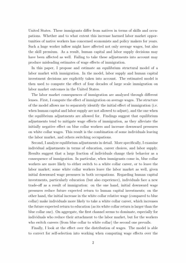
United States. These immigrants differ from natives in terms of skills and occu-

pations. Whether and to what extent this increase harmed labor market oppor-

tunities of native workers has concerned economists and policy makers for years.

Such a huge worker inflow might have affected not only average wages, but also

the skill premium. As a result, human capital and labor supply decisions may

have been affected as well. Failing to take these adjustments into account may

produce misleading estimates of wage effects of immigration.

In this paper, I propose and estimate an equilibrium structural model of a

labor market with immigration. In the model, labor supply and human capital

investment decisions are explicitly taken into account. The estimated model is

then used to compute the effect of four decades of large scale immigration on

labor market outcomes in the United States.

The labor market consequences of immigration are analyzed through different

lenses. First, I compute the effect of immigration on average wages. The structure

of the model allows me to separately identify the initial effect of immigration (i.e.

when human capital and labor supply are not allowed to adjust), and the one when

the equilibrium adjustments are allowed for. Findings suggest that equilibrium

adjustments tend to mitigate wage effects of immigration, as they alleviate the

initially negative effect on blue collar workers and increase downward pressures

on white collar wages. This result is the combination of some individuals leaving

the labor market, and others switching occupations.

Second, I analyze equilibrium adjustments in detail. More specifically, I examine

individual adjustments in terms of education, career choices, and labor supply.

Results suggest that a large fraction of individuals change their behavior as a

consequence of immigration. In particular, when immigrants come in, blue collar

workers are more likely to either switch to a white collar career, or to leave the

labor market; some white collar workers leave the labor market as well, given

initial downward wage pressures in both occupations. Regarding human capital

investments, particularly education (but also experience), individuals face a new

trade-off as a result of immigration: on the one hand, initial downward wage

pressures reduce future expected return to human capital investments; on the

other hand, the initial increase in the white collar relative wage (compared to blue

collar) make individuals more likely to take a white collar career, which increases

the future expected return to education (as its white collar return is larger than the

blue collar one). On aggregate, the first channel seems to dominate, especially for

individuals who reduce their attachment to the labor market, but for the workers

who switch careers (from blue collar to white collar) the second one prevails.

Finally, I look at the effect over the distribution of wages. The model is able

to correct for self-selection into working when computing wage effects over the

2

distribution of wages. The individuals that are pushed out from the labor market

by immigrants are not a random sample. Instead, least productive workers will be

more likely to abandon the labor force. As a result, wage effects at the the lower

tail of the distribution will be underestimated if we compare accepted wages with

and without immigration. The model, however, allows me to compare wage offers

instead of accepted wages, thus correcting this downward bias in a very natural

way. Results suggest important biases for all quantiles below the median, which

become especially severe below the 20th percentile.

The framework builds on the equilibrium models described in Heckman, Lochner

and Taber (1998), Lee (2005), and Lee and Wolpin (2006, 2010). The supply side

of the model is similar to Keane and Wolpin (1997), which I extend to accom-

modate immigrant and native workers separately. Individuals live from age 16

to 65 and make yearly forward looking decisions on education, participation and

occupation. Human capital accumulates throughout the life-cycle both because

of investments in education, and because learning-by-doing on the job leads to

accumulation of (occupation-specific) work experience.

On the demand side, blue collar and white collar labor is combined with capital

to produce a single output. Labor is defined in skill units, which implies that work-

ers have heterogeneous productivity depending on their education, occupation-

specific experience, place of birth, gender, foreign experience and unobservables.

I assume a nested Constant Elasticity of Substitution (CES) production function

that accounts for skill-biased technical change through capital-skill complementar-

ity (as in Krusell, Ohanian, Rios-Rull and Violante, 2000). Skill-biased technical

change is important because it is considered as an alternative mechanism for the

rise in the skill premium over the last four decades. Hence, not taking it into

account may potentially lead to attribute its effect on wages to immigration.

I fit the model to U.S. micro-data data from CPS and NLSY for the period 1967-

2007. I then use the estimated parameters to quantify the effect of immigration on

labor market outcomes. In order to do so, I define a counterfactual world without

large scale immigration in which the immigrant/native ratio is kept constant to

1967 levels. Then, I compare counterfactual wages, human capital, and labor

supply with baseline simulations using the estimated parameters.

There is a large literature studying the effect of immigration on wages. The first

and the most prolific strand of the literature is the so-called spatial correlations

approach.1 The approach exploits the fact that immigrants cluster in a small

number of geographic areas, generating a large cross-city variation in immigrant

1 This strand of the literature was pioneered by Grossman (1982) and Borjas (1983), andnotably followed by Card (1990, 2001), Altonji and Card (1991), LaLonde and Topel (1991),Goldin (1994), Card and Lewis (2007), Saiz (2007), and Cortes (2008) among many others.

3

incursion. This variability can be used to identify how immigration relates to

wages. The key assumption is that metropolitan areas constitute closed labor

markets that are exogenously penetrated by immigrants. Borjas, Freeman and

Katz (1997), however, claim that natives may respond to the inflow of immigrants

by moving their labor to other cities until wages are equalized across areas.2

Closer to the approach used in the present paper, a more recent strand of the

literature changes the unit of analysis to the national level. Borjas, Freeman

and Katz (1992, 1997) put forward the “factor proportions approach” which has

evolved substantially in subsequent years. This methodology compares a nation’s

actual supply of workers in a particular skill group to counterfactual supply in

the absence of immigration. Initial studies borrowed elasticities of substitution

between different types of labor from the literature whereas in more recent studies,

beginning with Card (2001) and Borjas (2003), these elasticities are estimated.3

This literature typically assumes that labor supply is perfectly inelastic. As

a result, counterfactual labor supplies of workers in each skill group are pre-

dicted by simply removing immigrants from each cell. However, this assumption

is rather restrictive. Recent evidence suggests native responses to immigration.

Hunt (2012) uses cross-state variation to provide evidence that native children

might be encouraged to complete high school in order to avoid competing with

immigrant high school dropouts in the labor market. Smith (2012) finds that

immigration of low educated workers led to an important reduction of native em-

ployment, particularly severe for native youth. Peri and Sparber (2009) find that

natives specialize in language intensive tasks (occupations) to compensate by the

competition induced by immigrants in manual intensive occupations.

In the model presented below, individuals are allowed to adjust their human

capital and labor supply decisions. The structure of the model allows me to com-

pute more realistic counterfactual labor supplies taking individuals back to the

decisions they would have made without immigrants. Equilibrium adjustments

will tend to mitigate wage effects, and not taking them into account in the coun-

terfactuals may produce misleading results.

Dustmann, Frattini and Preston (2013) exploit variation at the regional level to

2 Borjas (2003) finds that negative effects of immigration on wages are smaller at the statethan at the national level, and Cortes (2008) finds state-level effects to be more sizable thanthose across metropolitan areas. Both conclude that negative effects are attenuated at the locallevel by native migration responses. Borjas et al. (1997), Card and DiNardo (2000), Card (2001),and Borjas (2006) analyze how immigration affects the joint determination of wages and internalmigration behavior. The magnitude of these responses, however, is a subject of controversy thatis out of the scope of this paper. Differentials in capital adoption are suggested by Lewis (2011)as an alternative mechanism.

3 More recent papers using this approach include Friedberg (2001), Card (2009), Ottavianoand Peri (2012), Manacorda, Manning and Wadsworth (2012), and Llull (2013) among others.

4

study the effect of immigration along the native wage distribution. Immigrants

are assumed to compete with individuals that are in a similar position in the

distribution. This redefinition of worker competition is important because the

authors find significant evidence of immigrant downgrading upon arrival. Given

this, their approach provides a better identification of which natives experience a

more intense competition by immigrants.

The framework presented in this paper allows for immigrant downgrading upon

arrival, and labor market competition is specified in terms of observable and

unobservable skills, as in Dustmann et al. (2013). The model below, however,

additionally corrects for biases generated by the self-selection into labor market

participation as described above, which is an important contribution of the paper.

The rest of the paper is organized as follows: Section I provides some descriptive

evidence; Section II presents the labor market equilibrium structural model with

immigration; Section III briefly introduces the solution and estimation algorithm;

in Section IV, I present parameter estimates and some validation exercises; Sec-

tion V presents the results for the counterfactual exercises. And Section VI con-

cludes.

I. Exploring U.S. mass immigration

According to Census data, the U.S. labor force was enlarged by about 26 millions

of working-age immigrants during the last four decades, an increase of almost

0.7 millions per year. This section aims to compare the evolution of the skill

composition of immigrants with that of natives, and to establish some correlations

between immigration, schooling, and occupational choice. These facts serve as a

motivation for the modeling decisions taken in subsequent sections.

According to Table 1, the share of immigrants in the population of working-age

increased from 5.7 to 16.6 percent over this period. The skill and occupational

composition of the immigrant inflow also changed substantially. The share of

immigrants among the less educated has increased faster than among any other

group (6.8% to 33.7%). And immigrants are increasingly more clustered in blue

collar jobs (6% to 24%, much larger than the 5.7% to 16.6% overall increase).

This blue collar concentration holds as well conditional on educational levels. For

example, the share of immigrants among dropout blue collar workers increased

from 7.2 to 55.5 percent, whereas it only increased from 6.8 to 33.7 percent for

the overall high school dropouts group.

These facts are analyzed in more depth in Appendix A. Three important ex-

tensions are shown there. First, the fact that immigrants are increasingly less

educated than natives is the result of a slower increase (as opposed to a reduc-

tion) in their education compared to natives. Second, the pattern of clustering

5

Table 1—Share of Immigrants in the Population (%)

1970 1980 1990 2000 2008

A. Working-age population 5.70 7.13 10.27 14.62 16.56

B. By education:High school dropouts 6.84 9.60 17.93 29.02 33.73High school graduates 4.32 5.14 7.94 12.04 13.27Some college 5.14 6.63 7.92 9.96 11.65College graduates 6.48 8.02 10.60 14.59 16.92

C. In blue collar jobs:All education levels 6.03 7.83 11.21 17.53 24.07High school dropouts 7.18 12.18 23.75 41.03 55.45High school graduates 4.19 4.94 7.57 12.47 17.30Some college 5.95 6.14 7.26 9.82 14.07College graduates 9.53 9.52 12.14 17.89 23.82

Note: Figures in each panel indicate respectively the percentage of immigrants in the populationworking-age, in the pool of individuals with each educational level, and among blue-collar workers.Sources: Census data (1970-2000) and ACS (2008).

in blue collar occupations holds at a more disaggregate level; therefore, although

sometimes the blue/white collar classification is seen as too broad and heteroge-

neous (especially for a long period of time), in this case it seems enough to describe

the differential supply shock across occupations. And, third, the national origin

composition of the immigrant stock changed gradually over the period: from a

majority of Western immigrants during 1960s and 1970s to a majority of Latin

Americans later on, and a substantial increase in immigration from Asia/Africa

in recent years. These changes in the national origin of immigrants can explain

most of the slower increase in education by immigrants.

Borjas (2003) compares immigration and wages in different education-experience

cells (see Borjas, 2003, Secs. II-VI). He considers four education groups and eight

(potential) experience categories to define cells that are then treated as closed

labor markets. As the incidence of immigration varies across skill groups, he

uses this variation to identify the effect of immigration on wages in regressions

that include different combinations of fixed effects. With this approach, he finds

a sizeable negative correlation between immigration and wages. I replicate his

results using 1960-2000 Censuses and 2008 ACS in Panel A from Figure 1. The

figure shows that the correlation between the share of immigrants in a skill cell and

the average wage of native males in that cell (net of fixed effects) is negative. In

particular, a one percentage point increase in the share of immigrants is associated

with a 0.41 (s.e. 0.044) percent decrease in the average hourly wage.

Given the research question of this paper, it is worthwhile to look at the corre-

lation between immigration and education. Panel B in Figure 1 compares school

enrollment rates and immigrant shares, following an analogous approach to the

6

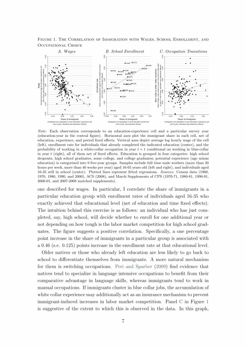
Figure 1. The Correlation of Immigration with Wages, School Enrollment, and

Occupational Choice

A. Wages

−0.

15−

0.10

−0.

050.

000.

050.

100.

15(n

et o

f yea

r, e

duca

tion

and

expe

rienc

e ef

fect

s)

−0.10 0.00 0.10 0.20 0.30

Share of immigrants

Ave

rage

log

hour

ly w

age

by e

duca

tion−

expe

rienc

e ce

llW

age

Immigrants over population in each education−experience cell(net of year, education and experience effects)

B. School Enrollment

SH70

SH80

SH60

SC08

SC00

HS08

HS00

CG00

CG08

SC90

CG90

HS90

CG60

SH90

HS80

CG80

CG70

HS60

HS70

SC80

SC60

SC70

SH00

SH08

−0.

07−

0.05

−0.

030.

000.

030.

05(n

et o

f yea

r, a

nd e

duca

tion

effe

cts)

−0.05 −0.03 0.00 0.03 0.05 0.07

Share of immigrants

Sha

re o

f you

ng p

opul

atio

n (a

ged

16−

35)

enro

lled

at s

choo

l

Enr

ollm

ent r

ate

Immigrants over population in each education−period cell(net of year, and education effects)

C. Occupation Transitions

−0.

10−

0.05

0.00

0.05

0.10

0.15

at y

ear

t+1

(net

of y

ear,

edu

catio

n an

d ex

perie

nce

effe

cts)

−0.10 0.00 0.10 0.20

Share of immigrants

Sha

re o

f blu

e−co

llar

wor

kers

at y

ear

t tha

t wor

k in

whi

te c

olla

rB

lue−

colla

r to

whi

te−

colla

r tr

ansi

tions

Immigrants over population in each education−experience cell(net of year, education and experience effects)

Note: Each observation corresponds to an education-experience cell and a particular survey year(education-year in the central figure). Horizontal axes plot the immigrant share in each cell, net ofeducation, experience, and period fixed effects. Vertical axes depict average log hourly wage of the cell(left), enrollment rate for individuals that already completed the indicated education (center), and theprobability of working in a white-collar occupation in year t + 1 conditional on working in blue-collarin year t (right), all of them net of fixed effects. Education is grouped in four categories: high schooldropouts, high school graduates, some college, and college graduates; potential experience (age minuseducation) is categorized into 9 five-year groups. Samples include full time male workers (more than 20hours per week, more than 40 weeks per year) aged 16-65 years old (left and right), and individuals aged16-35 still in school (center). Plotted lines represent fitted regressions. Sources: Census data (1960,1970, 1980, 1990, and 2000), ACS (2008), and March Supplements of CPS (1970-71, 1980-81, 1990-91,2000-01, and 2007-2008 matched supplements).

one described for wages. In particular, I correlate the share of immigrants in a

particular education group with enrollment rates of individuals aged 16-35 who

exactly achieved that educational level (net of education and time fixed effects).

The intuition behind this exercise is as follows: an individual who has just com-

pleted, say, high school, will decide whether to enroll for one additional year or

not depending on how tough is the labor market competition for high school grad-

uates. The figure suggests a positive correlation. Specifically, a one percentage

point increase in the share of immigrants in a particular group is associated with

a 0.46 (s.e. 0.125) points increase in the enrollment rate at that educational level.

Older natives or those who already left education are less likely to go back to

school to differentiate themselves from immigrants. A more natural mechanism

for them is switching occupations. Peri and Sparber (2009) find evidence that

natives tend to specialize in language intensive occupations to benefit from their

comparative advantage in language skills, whereas immigrants tend to work in

manual occupations. If immigrants cluster in blue collar jobs, the accumulation of

white collar experience may additionally act as an insurance mechanism to prevent

immigrant-induced increases in labor market competition. Panel C in Figure 1

is suggestive of the extent to which this is observed in the data. In this graph,

7

immigrant shares in education-experience cells are related to one year blue collar

to white collar transition probabilities in an analogous way to Panel A. The fitted

regression suggests that a percentage point increase in the share of immigrants in

a cell is associated with a 0.15 (s.e. 0.045) percentage points increase in the one

year blue collar to white collar transition probability. This effect is sizable, as it

suggests that the increase in immigration of the last decades would explain more

than a 10% of the observed increase in blue collar to white collar transitions. The

result is in line with the findings of Peri and Sparber (2009), and indicative of the

importance of taking into account occupational choice in the analysis.

The correlations presented in Panels B and C from Figure 1 are suggestive

of natives making adjustments to immigration in terms of human capital and

labor supply. However, career paths and human capital investments are forward

looking decisions that are difficult to asses through reduced form approaches. For

this reason, the model below describes the behavior of forward looking agents

making such decisions, within an equilibrium framework that links the effect of

immigration to native decisions through changes in relative wages.

II. A labor market equilibrium model with immigration

In this section, I present a labor market equilibrium model with immigration.

The model, estimated with U.S. data, is then used to quantify the effect of the

last four decades of immigration on wages, human capital, and labor supply of

incumbent workers (natives and previous immigrants).4 The main contribution of

this approach is to explicitly model labor supply and human capital decisions. It

also takes into account skill-biased technical change (considered as an alternative

hypothesis for the increase in wage dispersion in the U.S. in recent decades).

A. Career decisions and the labor supply

Native individuals enter in the model at age a = 16, and immigrants upon

arrival in the United States. They decide every year (until the age of 65 when

they die with certainty) among four mutually exclusive alternatives to maximize

their lifetime expected utility. The alternatives are: to work in a blue collar job,

da = B; or in a white collar job, da = W ; to attend school, da = S; or to stay at

home, da = H. There are L types of individuals that differ in skill endowments

and preferences, as described below. These types are defined based on observ-

able characteristics. Natives differ by gender (males and females). Immigrants

additionally differ in the region of birth (Western countries, Latin America, and

4 In order to make the text shorter and easier to read, I often use “native adjustments” in-distinctly to refer to adjustments by native individuals and adjustments by natives and previousimmigrants. The specific meaning in each case is easily identifiable from the context.

8

Asia/Africa). Hence, I assume six types of immigrants and two types of natives.

Immigrants enter the U.S. exogenously and with a given skill endowment. This

assumption is standard in the literature.5 Attempting to endogenize migration in

this model is not feasible for computational reasons, and because it would require

information on immigrants before and after migration, which is not available.6

At every point in time t, an individual i of type l and age a solves the following

dynamic programming problem:

Va,t,l(Ωa,t) = maxda

Ua,l(Ωa,t, da) + βE [Va+1,t+1,l(Ωa+1,t+1) | Ωa,t, da, l] , (1)

where the terminal value is V65+1,t,l = 0 ∀l, t.7 β is a subjective discount factor,

and Ωa is the information set of individual i at age a and time t (state variables are

listed below). The instantaneous utility function is choice-specific, Ua,l(Ωa, da =

j) ≡ U ja,l for j = B,W, S,H. Workers are not allowed to save and, hence, they

are not able to smooth consumption; as a result, I prevent them from having

incentives to smooth by assuming a linear utility function.

Working utilities are given by

U ja,t,l = wja,t,l + δBWg 1da−1 = H j = B,W, (2)

where wja,t,l are individual wages in occupation j = B,W , 1A denotes the

indicator function, which takes the value of one if condition A is satisfied and zero

otherwise, and δBWg is a gender-specific search cost that individuals have to pay

to get a job if they were not working (and not in school) in the previous period.8

Wages are defined as the product of the number of individual skill units times

their market price: wjt,a,l ≡ rjt × sja,l. Market prices of skill units, rjt , are obtained

in equilibrium, and individual skill units are defined by the individual-specific

component of a fairly standard Mincer equation (Mincer, 1974):

wja,t,l = rjt expωj0,l+ωj1,isEa+ω

j2XBa+ω

j3X

2Ba+ω

j4XWa+ω

j5X

2Wa+ω

j6XFa+ε

ja., (3)

where (εBa

εWa

)∼ i.i.N

([0

0

],

[(σBg )2 ρBWσBg σ

Wg

ρBWσBg σWg (σWg )2

]).

5 A recent exception to this is Llull (2013), who exploits exogenous variation from origincountries together with distance (using a two-sample two-stage least squares approach).

6 Computational complexity and data requirements for the estimation of structural modelsof migration decisions are discussed in Kennan and Walker (2011) and Lessem (2013).

7 For notational simplicity, I omit the individual subindex i, which should be present in allindividual variables throughout the paper. I do not include time subindex t in individual-specificvariables as long as, for a given individual i, t and a are perfectly collinear.

8 I assume that transitions from school into work are costless. Equivalently, new immigrantshave to pay this search cost unless they were at school in their home country in the previousperiod, i.e. if their foreign potential experience is strictly greater than zero.

9

The exponential part of equation (3) is the individual production function of

skill units, sja,l. All ωjs, interpreted as technology parameters, represent the re-

turn to each observable characteristic in terms of productivity in occupation j.

Therefore, education Ea, blue collar and white collar effective experience in the

U.S. XB and XW , and (potential) experience abroad XF , affect workers’ pro-

ductivity. The return to education, ωj1,is, is allowed to differ for immigrants and

natives (is = nat, immig).9 Equation (3) also includes a type-specific constant,

ωj0,l, and an i.i.d. unobserved shock, εja, with gender-specific variance σjg2, and

(gender invariant) correlation between the shocks for the two working alterna-

tives ρBW . When individuals decide to work in occupation j they accumulate

occupation-specific work experience, Xja+1 = Xja + 1da = j, which produces a

return in the future in the form of additional productivity and, hence, wages.

Skill prices rjt are only identified up to a multiplying constant in equation (3).

Therefore, I impose the normalization ωj0,male,nat = 0. Given this normalization,

a skill price is interpreted as the average wage in occupation j of native male

workers that have zero years of education and zero years of experience at time t.

Equation (3) allows for assimilation of immigrants. LaLonde and Topel (1992)

define assimilation as the process whereby, between two observationally equivalent

immigrants, the one with greater time in the U.S. earns more. According to this

definition, immigrants assimilate as they accumulate some skills in the U.S. that

they would not have accumulated in their home country (Borjas, 1999). In terms

of the present model, assimilation would be provided by a different (larger) return

to one year of U.S. experience compared to one year of experience abroad.10

Individuals who decide to attend school face a monetary cost, which is different

for undergraduate (τ1), and graduate students (τ1 + τ2). Additionally, they get a

non-pecuniary utility with a permanent component δS0,l, a disutility of coming back

to school if they were not in school in previous period δS1,g, and an i.i.d. transitory

shock εSa , normally distributed with gender-specific variance (σS)2g. Specifically,

USa,l = δS0,l − δS1,g1da−1 6= S − τ11Ea ≥ 12 − τ21Ea ≥ 16+ εSa . (4)

As a counterpart, they increase their education, Ea+1 = Ea + 1da = S, which

provides a return in the future.

Finally, individuals deciding to remain at home perceive the following non-

9 The different return to schooling for immigrants and natives may be the result of immigrantsundertaking (part of) their education abroad (e.g. learning Chinese calligraphy may not be asuseful as learning English to work in the U.S.). Ideally, I would allow the return to the educationobtained the U.S. and abroad to differ; however, such information is not observable in the data.Therefore, it is the return to all education what is different for natives and immigrants.

10 Eckstein and Weiss (2004), using data for Israel, find that foreign experience is almostunvalued upon arrival, and that conditional convergence takes place as the immigrant keepsaccumulating local experience.

10

pecuniary utility:

UHa,t,l = δH0,l + δH1,gna + δH2,gt+ εHa . (5)

In this case, on top of its permanent and transitory components δH0,l and εHa ,

utility is increased by a gender-specific amount δH1,g for each preschool children

living at home, na.11 Additionally, I add a gender-specific trend δH2,gt to correct

for the linear utility assumption. A linear utility function implies no income effect

in the labor force participation decision, and, hence, everything is driven by the

substitution effect; in a framework with growing wages, everyone would eventually

end up working at some point. Including a linear trend in the utility is a reduced

form way to circumvent this problem.

B. Aggregate production function and the demand for labor

The economy is represented by an aggregate firm that produces a single output,

Yt, combining labor (blue collar and white collar labor skill units, SBt and SWt)

and capital (structures and equipment capital, KSt and KEt) with a technology

that is described by the following nested Constant Elasticity of Substitution (CES)

production function:

Yt = ztKλStαS

ρBt + (1− α)[θSγWt + (1− θ)Kγ

Et]ρ/γ(1−λ)/ρ. (6)

Equation (6) is a Cobb-Douglas production function that combines structures with

a composite of labor and equipment capital. This composite is a CES aggregate

that combines blue collar labor with another CES aggregate of equipment capital

and white collar labor. Neutral technological progress is provided by the aggregate

productivity shock zt. Parameters α, θ, and λ are connected with the factor shares,

and ρ and γ are related to the elasticities of substitution between the different

inputs. The elasticity of substitution between equipment capital and white collar

labor is given by 1/(1− γ), and the elasticity of substitution between equipment

capital or white collar labor and blue collar labor is 1/(1− ρ).

Skill units are supplied by workers according to equation (3). As individuals

are not allowed to save, capital and output are taken from the data. Given that

capital stocks are equilibrium quantities, the implicit assumption is that labor

supply only affects capital through changes in the aggregate labor supply, but not

through the distribution of skills; likewise, only the aggregate capital stock, but

not the distribution of assets, have an effect on labor supply.12

11 The variable na is assumed to take one of the following values: 0, 1 or 2 (the latter for 2or more children). Fertility is exogenous (transition probability matrix is taken from the data)and depends on gender, education, age and cohort (see Appendix C).

12 This assumption is relevant for the counterfactual exercises in Section V. Counterfactualcapital in the absence of immigration is required to correctly asses the effect of immigration onwages. To account for this, I simulate different scenarios for counterfactual capital.

11

The aggregate productivity shock zt is obtained as the residual in equation (6).13

Its evolution is assumed to be described by the following autoregressive model:

ln zt+1 − ln zt = φ0 + φ1(ln zt − ln zt−1) + εzt+1, εzt+1 ∼ N (0, σ2z). (7)

This process allows for a constant exogenous productivity growth rate, and busi-

ness cycle fluctuations around it.

I abstract from modeling the effect of immigration on the demand of the pro-

duced good and its equilibrium feedback on wages. Two assumptions are consis-

tent with this: perfectly inelastic product demand (i.e. a tradable good whose

price is fixed at international goods market) or that immigration increases the

size of the market for the produced good proportionally to how it increases the

labor force. The latter seems plausible at the aggregate level —at a more dis-

aggregate level, there is some evidence suggesting that immigration affected the

price of some goods more than others (e.g. Cortes, 2008). The implications of this

assumption are discussed in Borjas (2009).

Economic theory suggests that immigration affects wages by lowering the wage

of competing workers (Borjas, 1999). As argued by Dustmann et al. (2013), how-

ever, the definition of competing workers should take into account that immigrants

often downgrade at entry. The analysis at the occupational level is convenient in

this context. A foreign engineer working in a farm is not competing with a native

professional engineer, but with a native farmer. As discussed in Section I, natives

and immigrants concentrate in different occupations given observable skills, and

foreign workers are increasingly more clustered in blue collar jobs. Additionally,

it is easier for workers to switch occupations than skills as a mechanism to over-

come immigrant competition. Peri and Sparber (2009) argue that immigration

caused natives to reallocate their task supply, thereby reducing downward wage

pressures. Kambourov and Manovskii (2009) model the importance of switching

occupations in explaining the increase in wage inequality.

Blue collar and white collar workers are broad groups. As mentioned in Section I,

however, these two categories seem to be narrow enough to describe the differential

supply shock across occupations in this context. The larger the number of skill

prices, the more heterogeneous effects of immigration on wages will be allowed for

in the model. However, the computational burden increases with the number of

skill prices to be solved in equilibrium.14

13 As zt affects labor supply decisions though its effect on wages, this aggregate shock needsto be jointly determined with aggregate skill units. This joint determination is solved as a fixedpoint problem, as described in Section III.

14 The state space of the individual maximization problem increases exponentially with thenumber of aggregate variables and prices. Additionally, the cost of solving for equilibrium skillprices also increases with the number of prices to be solved for. And, finally, the complexity of

12

Equation (6) is different from the three-level nested CES proposed by Card and

Lemieux (2001) that has become popular in the immigration literature since its

introduction by Borjas (2003). This production function proposes a technology

that is a Cobb-Douglas combination of capital and a labor aggregate. Labor is a

CES aggregation of four educational cells, each being itself a CES aggregate over

five experience cells. Labor supply in each education-experience cell is computed

as worker counts. Equation (6) differs from the three-level nested CES in the

following aspects: (i) it adds the occupational layer; (ii) it allows for capital-skill

complementarity as a source of skill-biased technical change; (iii) the marginal rate

of substitution between two workers is increasing in the productivity gap between

them, even within occupations;15 and (iv) it implies solving for two equilibrium

prices instead of thirty-two (see footnote 14).16

Capital-skill complementarity is important to account for skill-biased technical

change. Krusell et al. (2000) use a production function similar to equation (6) to

link the decline in the relative price of equipment capital beginning in the early

70s (technical change), to the increase in the college-high school wage gap (skill-

biased). This link is provided by ρ > γ, meaning that equipment capital is more

complementary to skilled labor (in their paper college workers, in this paper white

collar workers) than to unskilled labor (high school or blue collar workers). As

a result, the increasing speed of accumulation of equipment capital —exogenous

in this model, but generated by the decline in its price as shown in Krusell et al.

(2000)— would increase the relative demand of white collar workers.

C. The equilibrium

The aggregate supply of skill units in occupation j = B,W is given by

Sjt =65∑

a=16

Na,t∑i=1

sja,i1da,i = j. (8)

where Na,t is the cohort size. The aggregate demand comes from the aggregate

firm’s profit maximization, which equalizes marginal returns to skill rental prices:

rSBt = (1− λ)α(ztK

λSt

) ρ1−λ Sρ−1

Bt Y1− ρ

1−λt , (9)

the expectation rules for individuals to forecast future skill prices is also affected by the numberof skill prices to be forecasted.

15 The three-level nested CES assumes that the elasticity of substitution between a highschool dropout worker and a college graduate is the same as the one between a high schooldropout and a high school graduate. In this model, although individual skill units are perfectsubstitutes within an occupation, workers are not (e.g. a one percent reduction in the numberhigh school dropouts needs to be replaced by a larger number of high school graduate workersthan of college graduates to keep output constant).

16 The thirty-two skill prices come from four education groups times eight experience groups.

13

rSW t = (1− λ)(1− α)θ(ztK

λSt

) ρ1−λ Sγ−1

Wt KWρ−γt Y

1− ρ1−λ

t , (10)

where KWt ≡ [θSγWt + (1 − θ)KγEt]

1/γ. The labor market equilibrium is given by

the skill prices —rjt for j = SB, SW— that clear the market of skill units.17

Given equations (9) and (10) we can write the (log of the) relative white collar

to blue collar skill price as:

lnrWt

rBt= ln

(1− α)θ

α+ (ρ− 1) ln

SWt

SBt+ρ− γγ

ln

(θ + (1− θ)

(KEt

SWt

)γ). (11)

Equation (11) can be interpreted as a reformulation of Tinbergen’s race between

technology and the supply of skills (Tinbergen, 1975).18 The second term of this

equation is the negative contribution of the relative supply of skills (provided

by ρ < 1) and the last term captures the biased technical change through the

speeding up in the accumulation of equipment capital (whenever ρ > γ).

Every year t, workers make a forecast of the future path of the information set in

the state points they expect to reach. The information set at year t, Ωa,t, is given

by the following state variables: age, education, blue collar and white collar effec-

tive work experience, foreign potential experience, previous year decision, calendar

year, number of children, idiosyncratic shocks, and skill prices. Among them, they

face uncertainty about future skill prices, number of children, and idiosyncratic

shocks. The fertility process is exogenous and (given education and age) known by

all agents, i.e. all individuals know the probability of having 0, 1 or 2+ children in

the next period conditional on the number of children today, their education, and

their age. Idiosyncratic shocks have no persistence. Therefore, the best forecast

is their conditional mean. The path of future skill prices is determined by the

sequence of aggregate variables and the aggregate shock. In order to forecast the

aggregate shock, individuals use the process given by equation (7). Forecasting

the sequence of aggregate variables is more complicated. The future supply of

aggregate skill units depends on the future distribution of state variables over the

population, whose sufficient statistic is its current distribution. Therefore, ratio-

nality implies that individuals use this current distribution of state variables to

forecast future skill prices. Handling such a distribution as a state variable is not

feasible in practice. To make the problem tractable, I follow an approach inspired

17 There are two additional first order conditions that deliver the demands for structures andequipment capital. Given equilibrium capital stocks (taken from the data), these two conditionsare irrelevant to solve the labor market equilibrium. However, they are used in counterfactualexercises in Section V to recover interest rates in the counterfactual scenario in which I assumeperfect capital adjustment.

18 Tinbergen (1975) suggests that the overall change in the gap between skilled and unskilledwages is driven by two contrasting forces: the relative increase in the supply of skills, whichtends to close the gap, and a skill-biased technical change, which opens it. Acemoglu (2002),and Acemoglu and Autor (2011) survey the literature that have tested this hypothesis.

14

by Krusell and Smith (1998) and Altug and Miller (1998), and similar to the one

in Lee and Wolpin (2006, 2010). More concretely, I approximate the expectation

rule for future skill prices using a subset of the information included in the current

distribution of state variables that contains most of the relevant information that

is needed to predict future skill prices: current skill prices. The following VAR

replicates fairly well the path of skill prices:

∆ ln rjt+1 = ηj0 + ηjB∆ ln rBt + ηjW∆ ln rWt + ηjz∆ ln zt+1. (12)

This rule is an approximation to rational expectations as long as the estimated

process provides the best fit to the data that is generated using the rule itself to

solve the individual maximization problem. In other words, it is a good approx-

imation to rational expectations if the estimated parameter vector η is a fixed

point of an algorithm that uses equation (12) to solve individuals’ problem and

to generate a sequence of equilibrium skill prices, and then updates its parameter

values estimating the equation with the generated data.

An additional aspect that is important for this paper is the forecasting of fu-

ture immigration. This forecasting is implicit in the estimated parameters η.

Therefore, I assume that individuals also form rational expectations on future

immigration, and that current skill prices are also a sufficient statistic for it.

III. Model solution and estimation

The equilibrium model presented in Section II does not have a closed form so-

lution and needs to be solved numerically. The solution and estimation algorithm

is explained in detail in Appendix B. Data sources and definitions are described

in Appendix C. In this section I briefly describe the intuition of the proposed

algorithm, and I highlight the main features of the data used in the estimation.

In order to give the intuition of the solution and estimation algorithm it is conve-

nient to differentiate two types of parameters: expectation parameters, Θ2, which

are given by the forecasting rules described in equation (12), and the process for

the aggregate shock (7), and fundamental parameters of the model, Θ1, which are

the remaining parameters described in Sections II.A and II.B. Forecasting rules

are part of the solution of the model, in the sense that their parameters η are

implicit functions of the fundamental parameters. Parameters from the aggre-

gate shock process are fundamental by nature, but since the aggregate shock is

estimated as a residual (i.e. an implicit function of the data and fundamental pa-

rameters), and it is used to forecast future skill prices in the same way forecasting

rules given by equation (12) are used, I treat (and estimate) them as expectation

parameters. We can express Θ2 as Θ2(Θ1).

15

Parameters in Θ1 are estimated by Simulated Minimum Distance. The Simu-

lated Minimum Distance estimator minimizes the distance between a large num-

ber of statistics from the data (or data points) and their simulated counterparts.

Θ2(Θ1) is obtained as the fixed point of an algorithm that simulate the behavior

of individuals using a guess of Θ2, and then estimates equations (7) and (12) from

the simulated data to update the guess. Therefore, the estimator requires a nested

algorithm with a procedure that estimates Θ1, and another solving Θ2 given Θ1.

Lee and Wolpin (2006, 2010) describe a natural nested algorithm in which an

inner procedure finds the fixed point in Θ2 for every guess of Θ1, and an outer

loop solves the Θ1 estimation problem with a polytope algorithm. The main

drawback of this procedure is that it requires solving the fixed point problem in

every evaluation of Θ1, and this increases the computational burden significantly.19

I propose an alternative algorithm that avoids having to solve the fixed point in

every iteration of Θ1. In particular, I propose a swapping of the two procedures

which is in the same spirit of the swapping of conditional choice probabilities

and parameter estimation proposed by Aguirregabiria and Mira (2002). Θ1 is

estimated for every guess of Θ2, which is updated at a lower frequency. In other

words, I estimate Θ1(Θ2) for every guess of Θ2 instead of the opposite.

The model is fitted to a large number of statistics computed with micro-data

from 1967 to 2007. These statistics are listed in Table B1 in Appendix B. Their

simulated counterparts are obtained by simulating the behavior of cohorts of 5,000

natives and 5,000 immigrants (some of them starting their life abroad and not

making decisions until they arrive in the U.S.). Cross-sectional simulated data

are, hence, calculated with a sample of up to 500,000 observations, which are

weighted using data on cohort sizes.

Additional data for exogenous variables is used in the solution of the model.

These variables include output, structures and equipment capital stocks, cohort

sizes (by gender and immigrant status), the distribution of entry age for immi-

grants, the distribution of initial schooling (at age 16 for natives and upon entry in

the U.S. for immigrants), the distribution of immigrants by region of birth, and the

fertility (preschool children) process. Their sources, definitions, and construction

are detailed in Appendix C.

Appendix B also discusses parameter identification. No formal proof is available,

but some intuition is provided. As an heuristic check Figure D1 in Appendix D

plots different sections of the objective function in which I move one parameter

19 This problem is relatively exacerbated if one uses the parallel version of the Simplex Methoddeveloped by Lee and Wiswall (2007) in the minimization problem. The basic idea in Lee andWiswall (2007) is to move the p worst parameters in each Simplex iteration. The problem isthat if one of the processors takes more iterations to find the fixed point in Θ2(Θ1) than allothers, the latter will remain idle while the former performs further iterations.

16

and keep the others constant to the estimated values. Although this exercise is

uninformative about the curvature in the multidimensional space, it shows plenty

of unilateral curvature for all parameters. Pointing in the same line, standard

errors of the estimates reported below are very small, which is significant because

they depend on the curvature of the objective function around parameter estimates

—see Appendix E. Regarding uniqueness, I started the estimation from different

initial conditions and kept the local minimum that gave a smaller value for the

objective function.

IV. Estimation results

A. Parameter estimates

In this Section, I discuss parameter estimates, presented in Table 2 and Table 3.

Standard errors, in parentheses, take into account both sampling error and a

simulation error (see details on their calculation in Appendix E).20

Fundamental parameters of the model. Panel A in Table 2 presents gen-

der × origin constants for each alternative. Women are less productive than men

in both occupations (to a larger extent in blue collar), obtain a larger utility from

attending school, and a smaller utility from staying at home; all this is consistent

with the observed wage gap, enrollment rates, and female concentration in white

collar occupations. Similarly, native-immigrant differentials in wages and home

utility mimic the corresponding wage gaps (none for Western immigrants, very

large for Latin Americans, and somewhere in between for Asian/African). Except

for Latin Americans, immigrants get a larger utility from schooling than natives,

which, although at the first glance may seem at odds with their lower enrollment,

is necessary to replicate their decisions given the large school reentry cost.

Estimates for wage equations are presented in Panel B. The return to an ad-

ditional year of schooling for natives is estimated to be 7.3% in blue collar occu-

pations and 11.0% in white collar. For immigrants, returns are smaller in blue

collar occupations (5.7%), and similar in white collar (11%). These estimates fit

within the variety of results surveyed by Card (1999), which range from 5 to 15%

with most of the estimated causal effects clustering between 9% and 11%; results

are also qualitatively in line with (although somewhat larger than) Keane and

Wolpin (1997), Lee (2005), and Lee and Wolpin (2006). Both blue collar and

white collar own experience are estimated to have a quadratic return. Returns to

cross experience are much lower, much flatter, and turn negative after few years

of experience. Standard deviations for male and for white collar wages are esti-

20 Standard errors from expectation rules and the aggregate shock process are regressionstandard errors instead of minimum distance standard errors.

17

Table 2—Parameters Estimates

Nat. Nat. Western Latin Asia/A. Origin×gender constants: male female countries America Africa

Blue collar 0 -0.338 0.086 0.046 -0.005(0.0010) (0.0292) (0.0169) (0.0060)

White collar 0 -0.292 0.157 -0.170 0.059(0.0015) (0.0355) (0.0169) (0.0140)

School 2,424 5,606 7,545 2,646 10,184(68) (84) (249) (249) (382)

Home 16,678 11,341 16,379 12,298 14,962(53) (29) (764) (240) (143)

B. Wage equations: Blue collar White collar

Education—Natives (ω1,nat) 0.073 (0.0001) 0.110 (0.0001)Education—Immigr. (ω1,imm) 0.058 (0.0005) 0.110 (0.0005)BC Experience (ω2) 0.094 (0.0001) 0.001 (0.0003)BC Experience squared (ω3) -0.0023 (0.00018) -0.0005 (0.00016)WC Experience (ω4) 0.029 (0.0000) 0.105 (0.0000)WC Experience squared (ω5) -0.0013 (0.00001) -0.0029 (0.00001)Foreign Experience (ω6) 0.018 (0.0005) -0.046 (0.0012)

Variance-covariance matrix of i.i.d. shocks:

Std. dev. male (σmale) 0.443 (0.0058) 0.547 (0.0039)Std. dev. female (σfemale) 0.392 (0.0024) 0.492 (0.0035)Correlation coefficient (ρBW ) 0.062 (0.0052)

C. Utility parameters: Male Female

Labor market reentry cost (δBW1 ) 8,851 (76) 12,442 (180)

School utility parameters:

Undergraduate Tuition (τ1) 12,584 (85)Graduate Tuition (τ1 + τ2) 33,541 (869)Disutility of school reentry (δS1 ) 30,829 (207) 33,465 (597)

Home utility parameters:

Children (δH1 ) -1,775 (47) 3,663 (75)Trend (δH2 ) 55.59 (0.73) 52.68 (0.54)

Standard dev. of i.i.d. shocks:

School (σS) 1,280 (9) 1,339 (9)Home (σH) 10,437 (651) 5,011 (229)

Elast. of substit. param. Factor share parameters

D. Production function: BC vs Eq. (ρ) WC vs Eq. (γ) Struct. (λ) BC (α) WC (θ)

0.289 -0.067 0.091 0.547 0.444(0.006) (0.005) (0.013) (0.007) (0.010)

Autoregressive St. dev. ofE. Aggregate shock process: Constant (φ0) term (φ1) innovations (σz)

0.002 0.323 0.025(0.003) (0.115) (0.021)

Note: The table presents parameter estimates for equations (2) to (7). Native male constant for wageequations is normalized to zero. Immigrant male and native female constants are estimated. Theconstant for a female immigrant from region i is obtained as the sum of the constant for a male immigrantfrom region i and the difference between the constant for native females and native males. The individualsubjective discount factor, β, is set to 0.95. A more detailed description of each parameter can be foundin the main text. Standard errors (calculated as described in Appendix E) are in parentheses.

18

mated to be larger than for female and blue collar wages, mimicking the observed

pattern for variances in log wages. The correlation between the two shocks is

around 0.07, which pins down, together with returns to crossed-experience, the

observed transitions across occupations. Potential experience abroad is less pro-

ductive than own effective experience in the U.S. in both occupations. This lower

return generates conditional wage convergence for immigrants as they spend time

in the United States, which can be interpreted as immigrant assimilation in the

sense of LaLonde and Topel (1992). These results are in line with the findings in

Eckstein and Weiss (2004) for Israel.

Utility parameters are presented in Panel C. The labor market reentry cost is

estimated to be close to nine thousand US$ for males, and above twelve thousand

for females, which represent around one quarter and almost one half of the average

full-time equivalent annual wage for males and females respectively. Tuition fees

(as a difference from high school cost) are estimated to be slightly above twelve

thousand dollars for a bachelors degree, and around thirty-three for post-college, in

line with other estimates in the literature (e.g. Lee (2005), Lee and Wolpin (2006,

2010)). School reentry cost is quite large (close to the male average annual wage,

larger for females than for males), consistent with the rather unfrequent transitions

back to school observed in the data. Female obtain a larger additional utility than

male from staying at home when preschool children are present, replicating the

observed pattern of maternity/paternity leaves.21 The trend component of the

utility is estimated to be 52-55 U.S.$ per year, which despite being a modest

increase in relative terms (an overall utility increase of around 2, 100−2, 300U.S.$

over the sample years) is in line with the modest growth of the aggregate shock that

is generated by the model over this period. Variances of school i.i.d. idiosyncratic

shocks are somewhat small, whereas for the home alternative, they are larger, but

substantially smaller for female than for male.

Estimates for the production function parameters and the aggregate shock pro-

cess are presented in Panels D and E. Elasticities of substitution implied by ρ

and γ are respectively 1.41 and 0.94. These estimates imply that equipment cap-

ital and white collar labor are relative complements. This result —capital-skill

complementarity— is necessary to link the fast accumulation of equipment capital

and the increase in the white collar/blue collar (and college/high school) wage gap

(see equation (11)). Several papers have tested capital-skill complementarity with

different data since the seminal work by Griliches (1969). As noted by Hamermesh

(1986), although most of these studies agree in the existence of some degree of

21 Indeed, preschool children at home reduce male’s home utility. Given that individualsinstead of households are modeled, this negative parameter could be interpreted as male workingfurther to compensate for spouse’s maternity leave.

19

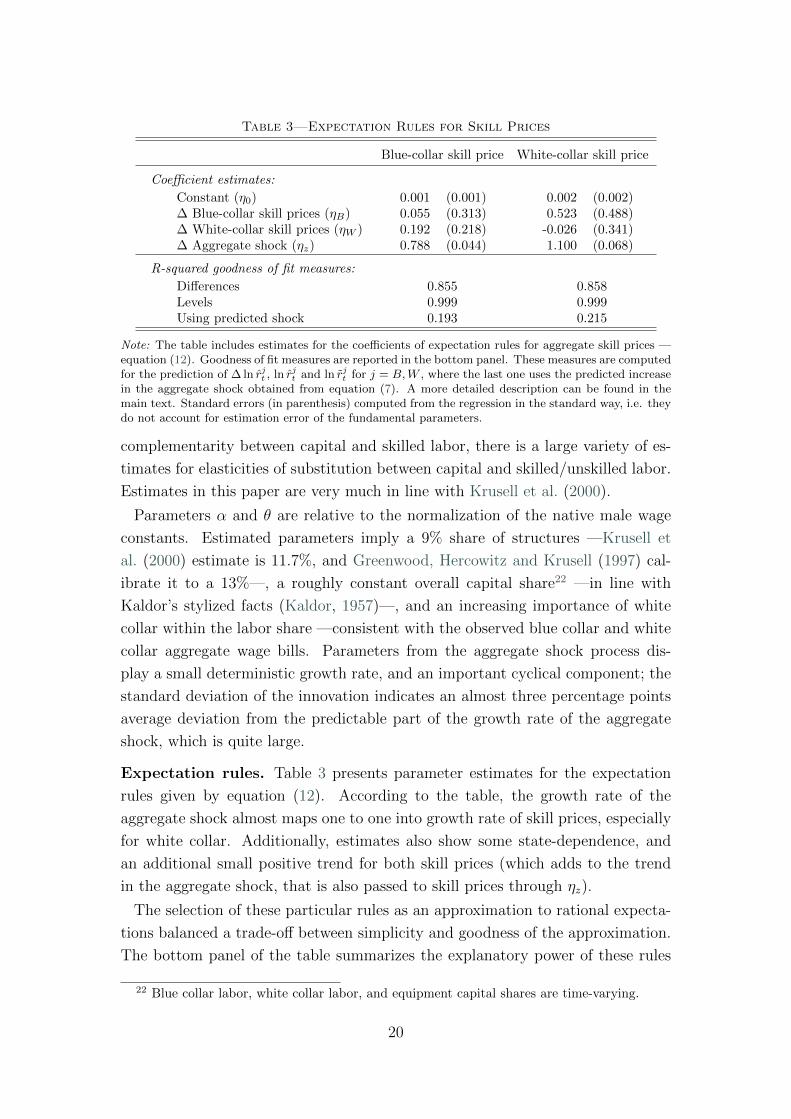
Table 3—Expectation Rules for Skill Prices

Blue-collar skill price White-collar skill price

Coefficient estimates:

Constant (η0) 0.001 (0.001) 0.002 (0.002)∆ Blue-collar skill prices (ηB) 0.055 (0.313) 0.523 (0.488)∆ White-collar skill prices (ηW ) 0.192 (0.218) -0.026 (0.341)∆ Aggregate shock (ηz) 0.788 (0.044) 1.100 (0.068)

R-squared goodness of fit measures:

Differences 0.855 0.858Levels 0.999 0.999Using predicted shock 0.193 0.215

Note: The table includes estimates for the coefficients of expectation rules for aggregate skill prices —equation (12). Goodness of fit measures are reported in the bottom panel. These measures are computedfor the prediction of ∆ ln rjt , ln rjt and ln rjt for j = B,W , where the last one uses the predicted increasein the aggregate shock obtained from equation (7). A more detailed description can be found in themain text. Standard errors (in parenthesis) computed from the regression in the standard way, i.e. theydo not account for estimation error of the fundamental parameters.

complementarity between capital and skilled labor, there is a large variety of es-

timates for elasticities of substitution between capital and skilled/unskilled labor.

Estimates in this paper are very much in line with Krusell et al. (2000).

Parameters α and θ are relative to the normalization of the native male wage

constants. Estimated parameters imply a 9% share of structures —Krusell et

al. (2000) estimate is 11.7%, and Greenwood, Hercowitz and Krusell (1997) cal-

ibrate it to a 13%—, a roughly constant overall capital share22 —in line with

Kaldor’s stylized facts (Kaldor, 1957)—, and an increasing importance of white

collar within the labor share —consistent with the observed blue collar and white

collar aggregate wage bills. Parameters from the aggregate shock process dis-

play a small deterministic growth rate, and an important cyclical component; the

standard deviation of the innovation indicates an almost three percentage points

average deviation from the predictable part of the growth rate of the aggregate

shock, which is quite large.

Expectation rules. Table 3 presents parameter estimates for the expectation

rules given by equation (12). According to the table, the growth rate of the

aggregate shock almost maps one to one into growth rate of skill prices, especially

for white collar. Additionally, estimates also show some state-dependence, and

an additional small positive trend for both skill prices (which adds to the trend

in the aggregate shock, that is also passed to skill prices through ηz).

The selection of these particular rules as an approximation to rational expecta-

tions balanced a trade-off between simplicity and goodness of the approximation.

The bottom panel of the table summarizes the explanatory power of these rules

22 Blue collar labor, white collar labor, and equipment capital shares are time-varying.

20

Figure 2. Actual and Predicted Education and Labor Supply

A. Average years of schooling 1

0 1

1 1

2 1

3 1

4

1967 1975 1983 1991 1999 2007

Years

of

educa

tion

Year

B. Participation rate

0 0

.25

0.5

0.7

5 1

1967 1975 1983 1991 1999 2007

Fract

ion w

ork

ing

Year

C. Share of workers in BC

0 0

.15

0.3

0.4

5 0

.6

1967 1975 1983 1991 1999 2007

Fract

ion in b

lue c

olla

r

Year

Actual/Male Actual/Female Predicted/Male Predicted/Female

Note: The figure plots observed and predicted average years of education (left), labor force participationrate (center), and fraction of employees working in blue collar occupations (right). The sample isrestricted to individuals aged 25-55. Actual data is obtained from March Supplements of the CPS(survey years from 1968 to 2008).

into three different R2 measures. The rules are able to predict around 86% of the

variation in growth rates of skill prices (top row), and display almost perfect fit

for the skill prices in levels (central row). This large explanatory power, however,

does not imply that individuals have perfect foresight of future skill prices, as

they do not observe zt+1 in period t. The third pseudo-R2 (bottom row) predicts

zt+1 using equation (7), as individuals do; this measure indicates that, in period

t, they are able to forecast around one fourth of the variation in (the growth rate

of) skill prices one period ahead, which, indeed, is far from perfect foresight.

B. Model fit

In this section, I compare predicted and actual values of the most relevant

aggregates for individuals aged 25 to 54 in order to evaluate the goodness of fit

of the estimated model. I focus on this age range because it is the one for which

I compare baseline and counterfactual outcomes in Section V.

Figure 2 plots actual and predicted statistics on education, labor force par-

ticipation and occupation. Panel A plots actual and simulated average years of

schooling for male and female.23 The model accuracy in predicting education for

males is remarkable: it predicts very well both the level and the increase in years

of schooling over the sample period. For females, the model accurately fits the

increase observed in the data (around 2.5 years), but slightly under-predicts the

level throughout (by around a third of a year). Panel B evaluates the goodness

of fit of the model in terms of labor force participation. The model does a good

prediction of the participation level, the increase in female labor force participa-

23 Average years of education are computed as follows: 0 if no education, preschool or kinder-garten, 2.5 if 1st to 4rth grade, 6.5 if 5th to 8th grade, 9, 10, 11, and 12 for the correspondinggrades, 14 for some college, and 16 for bachelors degree or more.

21

Figure 3. Actual and Predicted Experience Distributions

A. NLSY79

I. Blue Collar

0 0

.15

0.3

0.4

5 0

.6

0 2 4 6 8 10 12

Fract

ion o

f in

div

iduals

Years of experience

II. White Collar

0 0

.1 0

.2 0

.3 0

.4

0 2 4 6 8 10 12

Fract

ion o

f in

div

iduals

Years of experience

B. NLSY97

I. Blue Collar

0 0

.2 0

.4 0

.6 0

.8

0 1 2 3 4 5 6 7

Fract

ion o

f in

div

iduals

Years of experience

II. White Collar

0 0

.15

0.3

0.4

5 0

.6

0 1 2 3 4 5 6 7

Fract

ion o

f in

div

iduals

Years of experience


Note: The figure plots observed and predicted distribution of years of experience in blue collar andwhite collar accumulated by individuals from the NLSY samples. Experience is counted at the closestavailable year to 1993 (NLSY79) or 2006 (NLSY97).

tion, and the gender gap. It accurately predicts as well the level of male labor

force participation, although there is a minor discrepancy in replicating the trend

for this group as the model predicts a slightly increasing pattern, compared to

the roughly constant —rather slightly decreasing in early years— shape observed

in the data. Panel C compares actual and simulated fraction of employees work-

ing in blue collar occupations. The levels, the gender gap, and the decreasing

importance of blue collar occupations in both male and female employment are

replicated by the model. There is a slight under-prediction of the importance of

white collar in early years.

Figure 3 plots the actual and predicted distributions of blue collar and white

collar experience for individuals in the NLSY samples. For individuals in the

NLSY79 (Panel A), experience is measured around 1993, when individuals are

aged around 30. For the NLSY97 sample (Panel B), it is measured around 2006,

with individuals aged around 25. In general, the model generates experience

distributions with a very similar shape to their data counterparts.

Table 4—Actual vs Predicted Transition Probability Matrix

Choice in t

Blue collar White collar School Home

Choice in t− 1 Act. Pred. Act. Pred. Act. Pred. Act. Pred.

Blue collar 0.75 0.74 0.11 0.12 0.00 0.00 0.14 0.14White collar 0.06 0.07 0.83 0.83 0.00 0.00 0.10 0.10Home 0.11 0.08 0.13 0.12 0.01 0.01 0.76 0.79

Note: The table includes actual and predicted one-year transition probability matrix from blue collar,white collar, and home (rows) into blue collar, white collar, school, and home (columns) for individualsaged 25-55. Actual and predicted probabilities in each row add up to one. Actual data is obtained fromone-year matched March Supplements of the CPS (survey years from 1968 to 2008).

22

Figure 4. Actual and Predicted Wages

A. Average log hourly wages 2

2.3

2.6

2.9

3.2

1967 1975 1983 1991 1999 2007

Log h

ourl

y w

age

Year

B. College-high school wage gap

0 0

.15

0.3

0.4

5 0

.6

1967 1975 1983 1991 1999 2007

Diff

ere

nce

in log p

oin

tsYear

C. WC-BC wage gap

0 0

.15

0.3

0.4

5 0

.6

1967 1975 1983 1991 1999 2007

Diff

ere

nce

in log p

oin

ts

Year


Note: The figure plots observed and predicted average log hourly wages (left), college-high school wagegap (center) and white collar-blue collar wage gap (right). High school workers are those with 12 orless years of education, and college are those with more than 12 years. The sample is restricted toindividuals aged 25-55. Actual data is obtained from March Supplements of the CPS (survey yearsfrom 1968 to 2008).

The predictive power of the model in terms of transition probabilities is eval-

uated in Table 4. The table presents actual and predicted transition probability

matrix from blue collar, white collar, and home alternatives into blue collar, white

collar, school, and home.24 Transitions from the three alternatives are extremely

well replicated by the model. In particular, the model captures very well the

persistence in each of the alternatives, occupational switches, the fact that indi-

viduals rarely go back to school after leaving it, and transitions back and forth

from working to home.

Figure 4 evaluates the fit of the model in terms of wages. Panel A compares fitted

and actual average log hourly wages for male and female over the sample period.

The model predicts female wages very well; it also picks the level of male wages

and, hence, the gender wage gap. However, it is not able to replicate the hump

shape in the evolution of male wages observed between 1970 and 1990. This could

be the result of the rather simple parametrization of the aggregate production

function, or of not allowing returns to skills to vary over such a long period. Both

assumptions may have an effect on the identification of the aggregate shock, which

ultimately drives the evolution of wages. Panel B in Figure 4 compares actual and

predicted college-high school wage gap. The model clearly predicts the evolution

of the gap, with a slight decrease in early years and a sharp increase after mid

1970s. For females, although the evolution of the gap is well generated by the

model, the level is somewhat under-predicted. A fairly similar pattern can be

appreciated for the white collar-blue collar wage gap in Panel C.

So far, I have shown that model’s power in predicting the main aggregates is

24 Transitions from school into each of the four categories is omitted from the table becausevery few people is in school in the relevant age group (25-54).

23

Table 5—Out of Sample Fit: Act. vs Pred. Statistics for Immigrants

Out-of-sample In-sample

1970 1980 1990 1993-2007

Act. Pred. Act. Pred. Act. Pred. Act. Pred.

A. Male

Share with high school or less 0.67 0.61 0.57 0.56 0.52 0.54 0.55 0.56Average years of education 10.8 11.6 11.4 12.0 11.7 12.1 11.9 12.0Participation rate 0.77 0.64 0.68 0.67 0.63 0.71 0.75 0.75Share of workers in blue collar 0.57 0.55 0.55 0.53 0.53 0.52 0.58 0.52

B. Female

Share with high school or less 0.78 0.79 0.68 0.71 0.56 0.62 0.54 0.57Average years of education 10.3 10.7 10.9 11.4 11.5 11.9 12.0 12.2Participation rate 0.32 0.27 0.36 0.31 0.41 0.39 0.49 0.49Share of workers in blue collar 0.46 0.49 0.45 0.48 0.39 0.46 0.41 0.45

Note: The table presents actual and predicted values of four aggregate variables for immigrants. Statis-tics for 1993-2007 are obtained from March Supplements of the CPS, and are used in the estimation.Data for 1970, 1980, and 1990 are obtained from U.S. Census microdata samples and not used inthe estimation.

substantial. This conclusion is reached by comparing actual and simulated data

for several aggregate statistics. However, all these simulations are in-sample, in

the sense that they are the combination of different statistics used in the estima-

tion. Table 5 provides additional validation evidence to check the out-of-sample

predictive power of the model. In particular, I use the fact that, as it emerges

from Table B1 in Appendix B, statistics that are conditional on region of origin or

immigrant status of the individual are only available in the CPS starting in 1993.

Therefore, for the period before 1993, no separate information for natives and im-

migrants have been used in the estimation. Given that the fraction of immigrants

in the population working-age was below 10%, we can consider that the immigrant

group is small enough not to be driving the main aggregate trends. Moreover, as

discussed in Section I, the composition of immigrants in terms of education and

occupation diverged from that of natives over the years. And additionally, the fact

that the model replicates well immigrant behavior is crucial to correctly quantify

the size of the immigrant shock. The Table compares actual and predicted values

of four aggregate variables for immigrants —the share with high school diploma

or less, average years of education, participation rate, and the share of workers

employed in blue collar occupations— in 1969, 1979, and 1989. These data are

obtained from U.S. Census microdata samples for survey years 1970, 1980, and

1990 and not used in the estimation.25 The different statistics are compared sep-

arately for male and female. As it emerges from the table, the model does a good

job in predicting levels, trends, and gender gaps for the four aggregates.

25 Wages are not included in the table for comparability issues across databases.

24

V. Understanding the consequences of immigration:counterfactual exercises

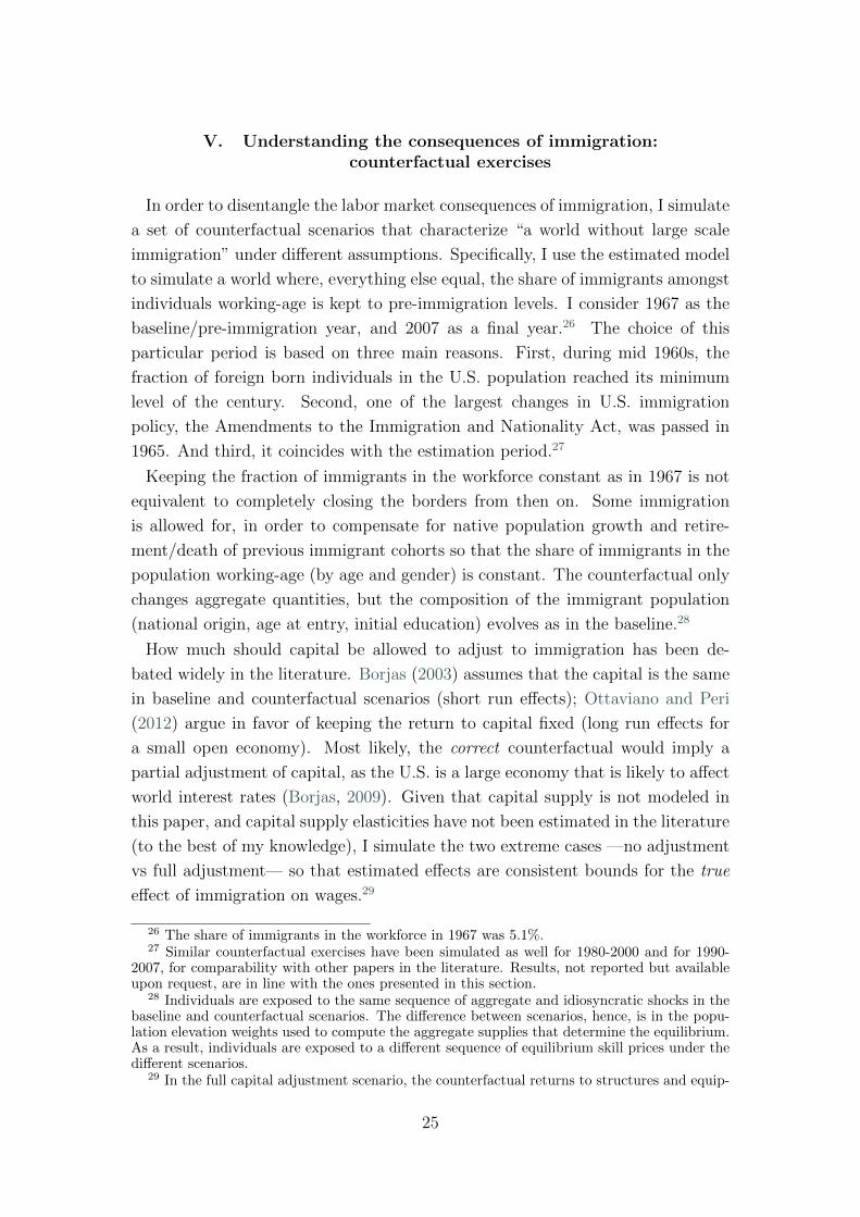
In order to disentangle the labor market consequences of immigration, I simulate

a set of counterfactual scenarios that characterize “a world without large scale

immigration” under different assumptions. Specifically, I use the estimated model

to simulate a world where, everything else equal, the share of immigrants amongst

individuals working-age is kept to pre-immigration levels. I consider 1967 as the

baseline/pre-immigration year, and 2007 as a final year.26 The choice of this

particular period is based on three main reasons. First, during mid 1960s, the

fraction of foreign born individuals in the U.S. population reached its minimum

level of the century. Second, one of the largest changes in U.S. immigration

policy, the Amendments to the Immigration and Nationality Act, was passed in

1965. And third, it coincides with the estimation period.27

Keeping the fraction of immigrants in the workforce constant as in 1967 is not

equivalent to completely closing the borders from then on. Some immigration

is allowed for, in order to compensate for native population growth and retire-

ment/death of previous immigrant cohorts so that the share of immigrants in the

population working-age (by age and gender) is constant. The counterfactual only

changes aggregate quantities, but the composition of the immigrant population

(national origin, age at entry, initial education) evolves as in the baseline.28

How much should capital be allowed to adjust to immigration has been de-

bated widely in the literature. Borjas (2003) assumes that the capital is the same

in baseline and counterfactual scenarios (short run effects); Ottaviano and Peri

(2012) argue in favor of keeping the return to capital fixed (long run effects for

a small open economy). Most likely, the correct counterfactual would imply a

partial adjustment of capital, as the U.S. is a large economy that is likely to affect

world interest rates (Borjas, 2009). Given that capital supply is not modeled in

this paper, and capital supply elasticities have not been estimated in the literature

(to the best of my knowledge), I simulate the two extreme cases —no adjustment

vs full adjustment— so that estimated effects are consistent bounds for the true

effect of immigration on wages.29

26 The share of immigrants in the workforce in 1967 was 5.1%.27 Similar counterfactual exercises have been simulated as well for 1980-2000 and for 1990-

2007, for comparability with other papers in the literature. Results, not reported but availableupon request, are in line with the ones presented in this section.

28 Individuals are exposed to the same sequence of aggregate and idiosyncratic shocks in thebaseline and counterfactual scenarios. The difference between scenarios, hence, is in the popu-lation elevation weights used to compute the aggregate supplies that determine the equilibrium.As a result, individuals are exposed to a different sequence of equilibrium skill prices under thedifferent scenarios.

29 In the full capital adjustment scenario, the counterfactual returns to structures and equip-

25

The results presented in this section are for native male aged 25-54. This par-

ticular subset of the population is targeted for two reasons: first, to make results

comparable to the existing literature; and second, to clean the estimated results

from confounding effects —e.g. some workers still in school at early ages, early

retirement for the oldest, and the change in female labor force participation over

the sample period. Results for other sub-populations are available upon request.

A. The effect of immigration on average wages

A crude approach to quantify the labor market effect of immigration is to look at

average wages. Table 6 presents the difference between baseline and counterfactual

average log wages and skill prices. In the top panel, counterfactual capital is

assumed to evolve as in the data (no adjustment); in the bottom panel, it is the

counterfactual return to capital what evolves as in the baseline (full adjustment,

if the United States were a small open economy). The left panel gives the raw

difference between counterfactual and baseline wages, and the right panel provides

the corresponding change in skill prices.

The first row from each panel presents the results of a counterfactual exercise in

which individuals are not allowed to adjust to immigration.30 This counterfactual

is equivalent to existing exercises in the literature (e.g. Borjas, 2003; Ottaviano

and Peri, 2012). The estimated effects under this approach suggest that the

observed increase in immigration between 1967 and 2007 reduced native male

average wages. In particular, results point to a fall in average wages induced by

immigration of 4.7% and 0.6% respectively in the two different capital scenarios.

The implied elasticities are -0.34 without capital adjustment (very much in line

with the estimates in Borjas (2003)) and -0.04 with full capital reaction (similar

to Ottaviano and Peri (2012)).31

Labor market adjustments are allowed for in the last row from each panel.

Results suggest that immigration reduced native male wages by 3% on average

if capital is not allowed to adjust. With full capital adjustment, immigration

increased average wages by 0.6%. The wage elasticities to immigration implied

ment capital are assumed to be the same as in the baseline so that the elasticity of the capitalsupply is infinity. The fact that the model delivers different returns to each of the two typesof capital is not necessarily inconsistent with the presence of a single world interest rate, asdepreciation rates of structures and equipment capital may differ.

30 In practice, this implies simulating baseline individual decisions, and then use counterfac-tual instead of baseline cohort sizes as population elevation weights to compute labor aggregatesin the terminal year. Then, using the resulting counterfactual labor supplies, skill prices areobtained from the first order conditions of the production function.

31 These elasticities are computed as the ratio between the percentage increase in wages(reported in the table) and the percentage increase in the workforce induced by immigration—i.e. (P2007 − P c

2007)/P c2007, where P2007 is the observed population working-age in 2007, and

P c2007 is its counterfactual counterpart—, which is 13.7%.

26

Table 6—Aggregate Effects and the Role of Equilibrium

Wages: Skill prices:

Average BC WC BC WC

No capital adjustment (∂K/∂m = 0):

No labor market adjustment -4.71 -6.12 -3.51 -6.12 -3.51Equilibrium effect 1.75 3.86 -1.77 3.49 0.20Total effect -2.96 -2.26 -5.28 -2.63 -3.30

Full capital adjustment (∂rK/∂m = 0):

No labor market adjustment -0.62 -2.90 1.32 -2.90 1.32Equilibrium effect 1.22 2.70 -1.41 2.76 -1.33Total effect 0.60 -0.20 -0.09 -0.14 0.00

Note: The table compares baseline and counterfactual average log wages and skill prices for native maleaged 25-55. Different panels correspond to different assumptions on counterfactual capital as indicated.“No labor market adjustment” indicates a scenario in which individuals are not allowed to adjust theirhuman capital, occupational choice, and labor supply. “Equilibrium effect” is the difference betweenthe total effect and the effect without labor market adjustment.

by these numbers are around -0.22 and 0.04 respectively. Therefore, labor market

equilibrium adjustments compensated the initial effect by 1.8 and 1.2 percentage

points respectively in the two capital scenarios —the difference between third

and first rows from each panel in Table 6, presented in the second row. These

differences indicate that labor supply adjustments mitigated the initial effect by

more than one third in the first case, and turned it into positive in the second.

The analysis at the occupational level, presented in the second and third columns

of Table 6, provides interesting insights. In the first row from each panel, we can

observe that, initially, blue collar wages are way more affected by immigration

than white collar wages. This is not surprising, given that immigrants tend to

cluster in blue collar jobs. What can be more surprising, though, is that after

labor market is allowed to adjust (third row), white collar wages are more affected

than blue collar ones. In particular, the magnitude of the effect on blue collar

wages decreases from 6.1% to 2.3% when capital is not allowed to adjust, whereas

the effect on white collar wages increases, from 3.5% to 5.3%. When capital is

allowed to adjust completely, these effects go from a 2.9% to a 0.2% decrease,

and from a 1.3% increase to a 0.1% decrease respectively. This result suggests

that some individuals adjust their decisions switching occupations and leaving the

labor market.

The mitigation of the initial effect of immigration can be explained by the com-

bination of three equilibrium mechanisms: changes in skills, composition effects,

and skill price adjustments after individuals’ re-optimization. Skill prices are the

primary channel through which immigration affects natives. The effect of immi-

gration on skill prices is analyzed in the right panel of Table 6. By construction,

with no labor market adjustment immigration affects skill prices and average

27

wages equivalently (Table 6, first row from each panel). After labor market ad-

justs, however, conclusions change. When capital does not adjust, the magnitude

of the effect on the blue collar skill price is reduced by almost four percentage

points, as so is the effect on average blue collar wage. However, the effect on

the white collar skill price is slightly mitigated, which is in contrast with the ex-

acerbation observed for the effect on average white collar wages. This different

behavior is the consequence of a change in the average skills of white collar and

blue collar workers after equilibrium adjustments, as discussed below.

B. Human capital and labor supply adjustments

The change in the average skill units of blue collar and white collar workers

can be the result of individual changes in skills and/or of composition effects.

Composition effects can be of different natures. Occupational switches are likely

to introduce less productive white collar workers into the pool, which reduces

average skills, whereas individuals dropping out from the labor force will typically

be the least productive ones, thus increasing the average. Changes in skills can

be the result of adjustments in education and/or in the experience accumulation

path. Two confronting forces are expected to work in this case: on the one hand,

if skill prices are initially reduced, the return to human capital investments is also

reduced, and, anticipating this, individuals may decide to invest less;32 on the

other hand, if a worker, as a result of the change in relative skill prices, is now

more likely to work in a white collar job, then she might decide to further invest

in education, as it is more rewarded in these occupations.

Table 7 compares individual baseline and counterfactual choices in the terminal

year, 2007. Even though the figures refer to a single year, they are the result

of a different exposure to immigration over several decades. The first column

presents the fraction of individuals that make different decisions in baseline and

counterfactual scenarios. The right panel presents the fraction of these individuals

switching to each of the three remaining alternatives.

When capital is not allowed to adjust, 13.8% of the individuals that would have

worked in a blue collar job in the absence of immigration do something else at the

observed immigration levels. Of them, almost one third decided to switch to a

white collar job, two thirds resigned to work, and a small fraction returned to (or

stayed longer at) school. Similarly, a 6.6% of otherwise white collar workers are

not such as a consequence of immigration; most of them decided to stay at home

instead. This sizeable detachment from the labor market in both occupations is

the consequence of both skill prices being reduced by immigration in this scenario.

32 Additionally, if the worker becomes more likely to spend some periods at home, the expectedreturn to human capital becomes even lower.

28

Table 7—Labor Supply Adjustments

Of which adjust to:

Fraction Blue White Home SchoolChoice w/o immigration adjusting collar collar


Blue collar 13.80 — 30.72 65.99 3.28White collar 6.60 5.20 — 90.93 3.87Home 0.94 13.08 67.39 — 19.54


Blue collar 8.24 — 56.31 41.84 1.85White collar 0.56 11.52 — 82.26 6.22Home 1.23 5.69 88.83 — 5.48

Note: The left column presents the percentage of native male aged 25-55 that make different choicesin baseline and in counterfactual simulations in the terminal year 2007. The right panel then presentsthe fraction of these individuals that switch to each of the three alternative choices. Top and bottompanels make different assumptions on counterfactual capital as indicated.

The fact that some individuals (around 4% — i.e., 30.7%×13.8%— of all otherwise

blue collar workers) switch from blue collar to white collar jobs is the result of the

initial effect on the relative skill prices.

If capital completely reacts, labor market adjustments are somewhat different.

A large fraction of the otherwise blue collar workers still adjust (8.2%), but very

few of the otherwise white collar workers (0.6%) do it. Indeed, even a 1.2% of

individuals who would not work otherwise, are now employed, mostly in white

collar jobs. These changes are the result of the smaller reduction of the blue

collar skill price, and the increase in the white collar one. Therefore, most of the

difference between the two capital scenarios comes from a smaller effect on labor

force participation. Now, more than a half of the otherwise blue collar workers

that changed their decision (still around a 4% of the total) switch to white collar,

whereas only forty percent of them (around 3.4% of the total, much lower than

the 9.1% in the no capital adjustment scenario) leave the labor market.

Table 7 suggests that immigration induces individuals to switch careers and/or

to detach from the labor market. The presented transition probabilities at the

terminal year provide an estimate of the probability of adjusting decisions as a

consequence of immigration. However, their main limitation is that they only refer

to a single period. As an alternative, Table 8 looks at career adjustments through

the lens of accumulated work experience. The table presents the fraction of native

male aged 25-54 that maintained, decreased, and increased their accumulated

experience after age twenty five. Additionally, it provides the fraction in each

group that increased white collar experience.

Results presented in the table confirm the findings in Table 7. Around 10-15% of

native males in the selected age range adjust their experience when capital is not

29

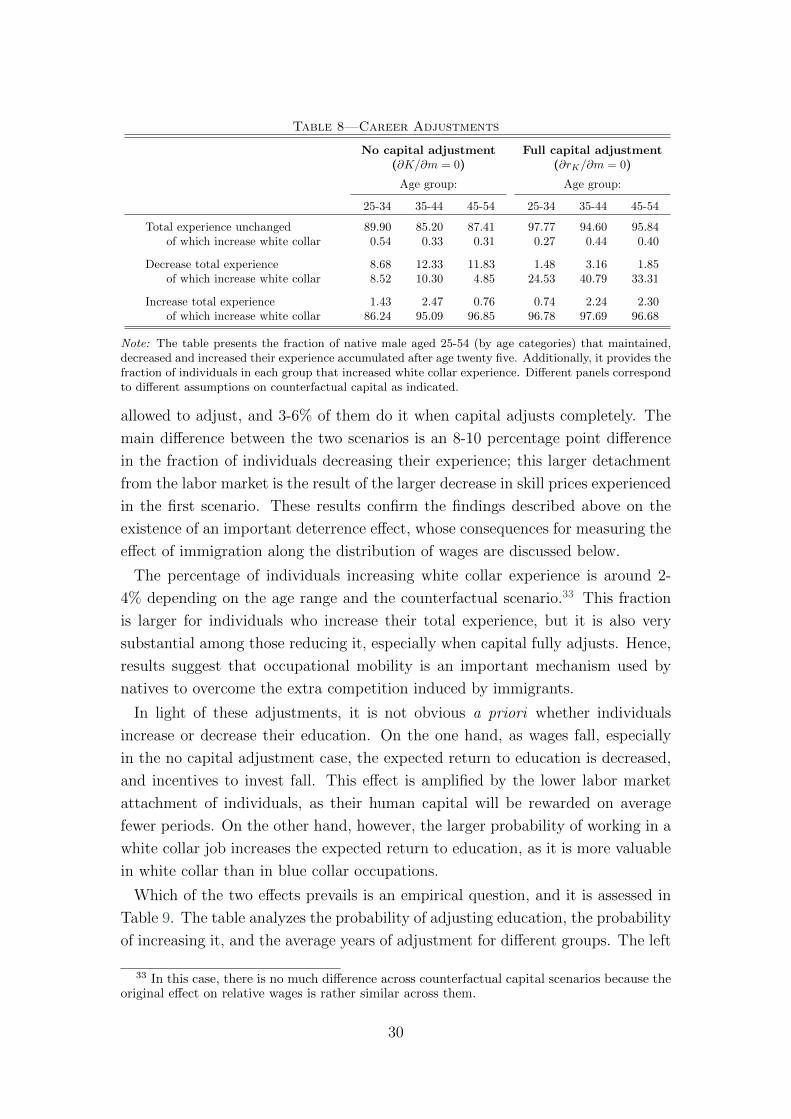
Table 8—Career Adjustments

No capital adjustment Full capital adjustment(∂K/∂m = 0) (∂rK/∂m = 0)

Age group: Age group:

25-34 35-44 45-54 25-34 35-44 45-54

Total experience unchanged 89.90 85.20 87.41 97.77 94.60 95.84of which increase white collar 0.54 0.33 0.31 0.27 0.44 0.40

Decrease total experience 8.68 12.33 11.83 1.48 3.16 1.85of which increase white collar 8.52 10.30 4.85 24.53 40.79 33.31

Increase total experience 1.43 2.47 0.76 0.74 2.24 2.30of which increase white collar 86.24 95.09 96.85 96.78 97.69 96.68

Note: The table presents the fraction of native male aged 25-54 (by age categories) that maintained,decreased and increased their experience accumulated after age twenty five. Additionally, it provides thefraction of individuals in each group that increased white collar experience. Different panels correspondto different assumptions on counterfactual capital as indicated.

allowed to adjust, and 3-6% of them do it when capital adjusts completely. The

main difference between the two scenarios is an 8-10 percentage point difference

in the fraction of individuals decreasing their experience; this larger detachment

from the labor market is the result of the larger decrease in skill prices experienced

in the first scenario. These results confirm the findings described above on the

existence of an important deterrence effect, whose consequences for measuring the

effect of immigration along the distribution of wages are discussed below.

The percentage of individuals increasing white collar experience is around 2-

4% depending on the age range and the counterfactual scenario.33 This fraction

is larger for individuals who increase their total experience, but it is also very

substantial among those reducing it, especially when capital fully adjusts. Hence,

results suggest that occupational mobility is an important mechanism used by

natives to overcome the extra competition induced by immigrants.

In light of these adjustments, it is not obvious a priori whether individuals

increase or decrease their education. On the one hand, as wages fall, especially

in the no capital adjustment case, the expected return to education is decreased,

and incentives to invest fall. This effect is amplified by the lower labor market

attachment of individuals, as their human capital will be rewarded on average

fewer periods. On the other hand, however, the larger probability of working in a

white collar job increases the expected return to education, as it is more valuable

in white collar than in blue collar occupations.

Which of the two effects prevails is an empirical question, and it is assessed in

Table 9. The table analyzes the probability of adjusting education, the probability

of increasing it, and the average years of adjustment for different groups. The left

33 In this case, there is no much difference across counterfactual capital scenarios because theoriginal effect on relative wages is rather similar across them.

30

Table 9—Changes in Education Conditional on Career Adjustments

Time at home is: Incr. WC experience:

Incr. Unch. Decr. T@H↑ T@H∼ T@H↓


% adjusting education 35.73 1.67 38.38 41.42 59.82 22.77of which increasing it 4.56 6.37 46.35 12.33 3.44 46.08

Average incr. education (years) -1.19 -0.03 0.25 -1.07 -1.04 0.30conditional on adjusting it -3.33 -1.62 0.65 -2.58 -1.74 1.33


% adjusting education 35.01 0.42 25.76 27.40 30.59 22.43of which increasing it 26.30 49.14 86.54 72.34 72.78 88.35

Average incr. education (years) -0.43 0.00 0.60 0.45 0.59 0.56conditional on adjusting it -1.23 0.43 2.31 1.65 1.92 2.48

Note: The first row from each panel presents the percentage of individuals in each subpopulation thathave different education in baseline and counterfactual scenarios; the second row is the percentageof these individuals that increased it as a consequence of immigration; the third row is the averageincrease in the number of years in the specific subpopulation; and the fourth is the average increase forindividuals adjusting it. Different columns refer to different subpopulations; columns in the left panelinclude individuals that increased, maintained, or decreased the time spent at home after age twentyfive respectively; columns in the right panel include the same groups for to individuals that increasedwhite collar experience. In all cases, the population of interest is native male aged 25-54. Top andbottom panels include different assumptions on counterfactual capital as indicated.

panel analyzes these outcomes depending on whether the individual increased,

decreased, or maintained the number of years spent at home after age twenty

five (indicated as T@H).34 Results suggest different patterns, depending on the

specific career adjustment. For individuals reducing their attachment to the labor

market (i.e., increasing the time spent at home), the first effect clearly prevails, as

they substantially reduce their education. In both scenarios, above one third of

the individuals adjust their education, most of them reducing it, with an average

reduction of 3.3 years with no capital adjustment, and 1.2 years with full capital

adjustment. This reduction is sizeable, as the total increase in average years of

education between 1967 and 2007 was around 2.5 years.

Conversely, not many of the individuals that do not adjust their career path

change their education as a consequence of immigration. Only 1.7% do so in the

no capital adjustment scenario, and 0.4% in the full capital adjustment. When

they do it, the first effect seems to dominate in the no capital adjustment scenario,

with an average reduction of 1.6 years, whereas the second slightly prevails in the

full capital adjustment scenario, consistent with the changes in skill prices in

34 Years spent at home after age twenty five and years of experience accumulated after thatage are mirror images, except for individuals that are still in school. Even though the focus onthe 25-54 age range limits substantially the presence of individuals in school, I opted for yearsat home to avoid creating a systematic relationship between increase in education and reductionof work experience in that situation. Results, available upon request, are roughly similar ifexperience instead of time at home is used.

31

each case. Nonetheless, the overall effect on the average education of the group

is negligible (-0.03 and less than 0.01 years respectively), given that only small

fraction of individuals adjusted.

Finally, for individuals increasing their attachment to the labor market the

second effect prevails, especially when capital fully reacts. In the no capital ad-

justment scenario, above one third of these individuals adjust their education,

although only about one half of them increase it. Yet, their average adjustment

is positive, of around 0.6 years. With full capital adjustment, among the almost

one quarter of individuals that adjust their education, most of them increase it.

On average, they increase their education by 2.3 years, which is again substantial.

The right panel replicates the same exercise restricting the sample to individuals

that increased their white collar experience as a consequence of immigration. In

this case, differences between capital scenarios are exacerbated. In the no capital

adjustment case, individuals that reduced their attachment to the labor market

(despite increasing their white collar experience), still reduce their education sub-

stantially. Similarly, those who increased their white collar experience without

altering the time spent at home also reduce their education.35 However, for indi-

viduals reducing time spent at home, their average increase in years of education

more than doubles the corresponding increase in the left panel. When capital fully

adjusts, between one quarter and one third of the individuals that increase their

white collar experience adjust their education, most of them increasing it. The

average increase in years of education for those adjusting is 1.7, 1.9. and 2.5 years

respectively depending on whether they increased, maintained, or decreased time

at home. This implies that, among individuals increasing their white collar expe-

rience, education increased on average by 0.5-0.6 years, one fifth of the observed

increase in the last four decades.

C. Self-selection and the effect of immigration along the wage distribution

Immigration does not affect all individuals in the same way. In Section I we

have seen that immigrants are less skilled than natives, and increasingly more

concentrated in blue collar occupations. Therefore, similar natives are likely to be

more affected by immigration. Dustmann et al. (2013) define similar individuals

depending on their position along the native wage distribution. This approach

has important advantages compared to assigning individuals to skill cells based on

observable characteristics, as the authors emphasize. It is also a natural approach

to analyze heterogeneous effects of immigration on wages of different individuals.

In a similar spirit, Figure 5 plots the effect of immigration along the distribu-

35 Results for this group should be interpreted with caution, as they could have increasedwhite collar experience at the expense of schooling.

32

Figure 5. Wage Effects Over the Wage Distribution

A. No capital adjustment

-0.2

-0.1

6-0

.12

-0.0

8-0

.04

0 0 20 40 60 80 100

Wage incr

ease

(lo

g p

oin

ts)

Percentile

B. Full capital adjustment

-0.0

6-0

.04

-0.0

2 0

0.0

2 0

.04

0 20 40 60 80 100

Wage incr

ease

(lo

g p

oin

ts)

Percentile

Accepted wages ±2 std. errors Offered wages ±2 std. errors

Note: The figure plots the average differences between log hourly wages in baseline and counterfactualscenarios for native male workers aged 25-54 along the baseline wage distribution. Each figure corre-sponds to a different assumption of the counterfactual evolution of capital as indicated. Black linesindicate the difference between baseline and counterfactual accepted wages. Gray lines indicates thedifference in accepted wages for all the individuals working in the no immigration case (counterfactual).

tion of wages of native male aged 25-54. Black solid lines represent the increase

in accepted wages induced by immigration in each percentile. Results differ de-

pending on the assumed counterfactual evolution of capital. If capital does not

adjust, immigration decreases wages by 2% at the top of the distribution, going

down to 7% at the bottom. With full capital adjustment, immigration increases

wages above the median, up to a 3% at the top of the distribution, whereas they

decrease wages below the median, up to a 1% at the bottom of the distribution.

One feature shared by the two scenarios is, hence, that individuals at the bottom

tail of the distribution are more negatively affected than individuals at the top.

This result is in line with the findings in Dustmann et al. (2013).

As the existing estimates in the literature, black lines in Figure 5 represent

the effect of immigration on accepted wages. Hence, baseline and counterfactual

wages are computed in each case with individuals that are working. Similarly,

Dustmann et al. (2013), compare observed wages at different points of the wage

distribution across regions that received different levels of immigration. However,

as Table 7 above suggests, some individuals abandoned the labor market as a

consequence of immigration. This labor market detachment is unlikely to be

random; instead, we would expect that individuals at the bottom tail of the

distribution are overrepresented among deterred individuals. Then, these results

may suffer from a self-selection bias.

One of the main advantages of the structural model estimated in this paper is

that it allows to naturally correct this bias. This is so because in the simulation of

the model, we observe wage offers in baseline and counterfactual scenarios. Addi-

tionally, as discussed in Section V.B, we observe the decisions made by individuals

33

under the different scenarios. Therefore, we can compute the effect of immigra-

tion on offered (instead of accepted) wages for all individuals that work in absence

of immigration. This comparison is depicted by gray lines in Figure 5. Results

show that self-selection bias severely affects estimates of wage effects below the

median. At the 5th percentile, the wage drop induced by immigration is substan-

tially larger once self-selection bias is corrected: from 7% to 20% in the no capital

adjustment scenario, and from 1% to 5% in the full capital adjustment case.

To the best of my knowledge, this is the first paper pointing to a self-selection

(participation) bias in the estimates of immigration on wages of less skilled work-

ers. And the bias appears to be very large. Therefore, these findings reinforce the

importance of taking into account labor market equilibrium adjustments when

analyzing the effect of immigration on wages.

VI. Concluding remarks

This paper estimates a labor market equilibrium model that takes into account

human capital and labor supply adjustments to immigration. These adjustments

are important to quantify the effect of immigration on wages. The model is esti-

mated by minimum distance using CPS and NLSY data for 1967-2007. The esti-

mated model is then used to measure the effect of immigration on wages simulating

a counterfactual world without the last four decades of large scale immigration.

Results suggest that the wage effects of immigration are very important initially,

but that they are then mitigated by equilibrium forces, as natives tend to adjust

their human capital and labor supply. When capital is not allowed to adjust in

the counterfactuals, native workers detach substantially from the labor market;

this effect is less severe when capital adjusts completely. Regarding human capital

(mainly education, but also work-experience) two opposite forces are at place: on

the one hand, downward wage pressures reduce the expected returns to human

capital; on the other hand, changes in relative wages make a white collar career

more attractive, which increases the expected return to education. On aggregate,

the first channel seems to dominate, especially for individuals that reduce their

attachment to the labor market, but the second prevails for individuals increasing

their labor market participation and for individuals switching to a white collar

career. Finally, immigration has heterogeneous effects on wages along the native

wage distribution. Self-selection out of the labor force produces important biases

in these estimates, especially at the lower tail. Results suggest negative effects

of immigration at the lowest percentiles, especially when the self-selection bias is

corrected for; at the top of the distribution, individuals are less affected or their

wages are even increased, depending on the assumption on counterfactual capital.

These results highlight the importance of taking human capital and labor sup-

34

ply adjustments into account when analyzing wage effects of immigration. This

opens interesting avenues for future research. The self-selection bias pointed in

Section V.C should be analyzed from different lenses, to gain more insight on its

implications for existing papers in the literature. Studying in more detail direct

and indirect effects of immigration on human capital, occupation specialization,

and employment decisions (along the lines of recent papers like Hunt (2012), Peri

and Sparber (2009), and Smith (2012)) would be interesting as well. Extending

the model to account for the role of endogenous migration decisions would be

another interesting line of future research. And, additionally, the framework of

this paper could be used to evaluate immigration policies for the United States.

The results from this paper improve our understanding of labor market conse-

quences of immigration in several dimensions, and have important implications

for policy design. However, policy makers should bear in mind that immigration

may affect the receiving society in other dimensions that are not included in the

current analysis. For instance, immigration may affect prices of goods and ser-

vices, taxes, welfare state, pension systems, or the use of public goods among

others. Our understanding of the consequences of immigration on some of these

outcomes is still limited.

REFERENCES

Acemoglu, D., “Technical Change, Inequality, and the Labor Market,” Journal

of Economic Literature, 2002, 40, 7–72.

and D. H. Autor, “Skills, Tasks and Technologies: Implications for Em-

ployment and Earnings,” in O. C. Ashenfelter and D. E. Card, eds., Handbook

of Labor Economics, Vol. 4B, Amsterdam: North-Holland, 2011, chapter 12,

pp. 1043–1171.

Aguirregabiria, V. and P. Mira, “Swapping the Nested Fixed Point Algo-

rithm: a Class of Estimators for Discrete Markov Decision Models,” Economet-

rica, 2002, 70, 1519–1543.

Altonji, J. G. and D. E. Card, “The Effects of Immigration on the Labor

Market Outcomes of Less-skilled Natives,” in J. M. Abowd and R. B. Freeman,

eds., Immigration, Trade and the Labor Market, Chicago: University of Chicago

Press, 1991, chapter 7, pp. 201–234.

Altug, S. and R. A. Miller, “The Effect of Work Experience on Female Wages

and Labor Supply,” Review of Economic Studies, 1998, 65, 45–85.

Becker, G. S., Human Capital. A Theoretical and Empirical Analysis, with Spe-

cial Reference to Education, New York: National Bureau of Economic Research,

1964.

35

Borjas, G. J., “The Substitutability of Black, Hispanic, and White Labor,”

Economic Inquiry, 1983, 21, 93–106.

, “The Economic Analysis of Immigration,” in O. C. Ashenfelter and D. E. Card,

eds., Handbook of Labor Economics, Vol. 3A, Amsterdam: North-Holland, 1999,

chapter 28, pp. 1697–1760.

, “The Labor Demand Curve Is Downward Sloping: Reexamining the Impact

of Immigration on the Labor Market,” Quarterly Journal of Economics, 2003,

118, 1335–1374.

, “Native Internal Migration and the Labor Market Impact of Immigration,”

Journal of Human Resources, 2006, 41, 221–258.

, “The Analytics of the Wage Effect of Immigration,” NBER Working Paper

n.14796, 2009.

, R. B. Freeman, and L. F. Katz, “On the Labor Market Impacts of Im-

migration and Trade,” in G. J. Borjas and R. B. Freeman, eds., Immigration

and the Work Force: Economic Consequences for the United States and Source

Areas, Chicago: University of Chicago Press, 1992, pp. 213–244.

, , and , “How Much Do Immigration and Trade Affect Labor Market

Outcomes?,” Brookings Papers on Economic Activity, 1997, 1997, 1–67.

Browning, M., A. Deaton, and M. Irish, “A Profitable Approach to Labor

Supply and Commodity Demands Over the Life-Cycle,” Econometrica, 1985,

53, 503–543.

Card, D. E., “The Impact of the Mariel Boatlift on the Miami Labor Market,”

Industrial and Labor Relations Review, 1990, 43, 245–257.

, “The Causal Effect of Education on Earnings,” in O. C. Ashenfelter and D. E.

Card, eds., Handbook of Labor Economics, Vol. 3A, Amsterdam: North-Holland,

1999, chapter 30, pp. 1801–1863.

, “Immigrant Inflows, Native Outflows, and the Local Labor Market Impacts of

Higher Immigration,” Journal of Labor Economics, 2001, 19, 22–64.

, “Immigration and Inequality,” American Economic Review: Papers and Pro-

ceedings, 2009, 99, 1–21.

and E. G. Lewis, “The Diffusion of Mexican Immigrants during the 1990s:

Explanations and Impacts,” in G. J. Borjas, ed., Mexican Immigration to the

United States, Chicago: University of Chicago Press, 2007, pp. 193–227.

and J. E. DiNardo, “Do Immigrant Inflows Lead to Native Outflows?,”

American Economic Review, 2000, 90, 360–367.

and T. Lemieux, “Can Falling Supply Explain The Rising Return To College

For Younger Men? A Cohort-Based Analysis,” Quarterly Journal of Economics,

2001, 116, 705–745.

36

Cortes, P., “The Effect of Low-Skilled Immigration on U.S. Prices: Evidence

from CPI Data,” Journal of Political Economy, 2008, 116, 381–422.

Dustmann, C., T. Frattini, and I. Preston, “The Effect of Immigration along

the Distribution of Wages,” Review of Economic Studies, 2013, 80, 145–173.

Eckstein, Z. and Y. Weiss, “On the Wage Growth of Immigrants: Israel 1990-

2000,” Journal of the European Economic Association, 2004, 2, 665–695.

Friedberg, R. M., “The Impact of Mass Migration on the Israeli Labor Market,”

Quarterly Journal of Economics, 2001, 116, 1373–1408.

Goldin, C., “The Political Economy of Immigration Restriction in the United

States, 1890 to 1921,” in C. Goldin and G. D. Libecap, eds., The Reglated

Economy: A Historical Approach to Political Economy, Chicago: University of

Chicago Press, 1994, pp. 223–257.

Greenwood, J., Z. Hercowitz, and P. Krusell, “Long-Run Implications of

Investment-Specific Technological Change,” American Economic Review, 1997,

87, 342–362.

Griliches, Z., “Capital-Skill Complementarity,” Review of Economics and Statis-

tics, 1969, 51, 465–468.

Grossman, J. B., “The Substitutability of Natives and Immigrants in Produc-

tion,” Review of Economics and Statistics, 1982, 64, 596–603.

Hamermesh, D. S., “The Demand for Labor in the Long Run,” in O. C. Ashen-

felter and D. E. Card, eds., Handbook of Labor Economics, Vol. 1, Amsterdam:

North-Holland, 1986, chapter 8, pp. 429–471.

Heckman, J. J., L. Lochner, and C. Taber, “Explaining Rising Wage In-

equality: Explorations with a Dynamic General Equilibrium Model of Labor

Earnings with Heterogeneous Agents,” Review of Economic Dynamics, 1998, 1,

1–58.

Hunt, J., “The Impact of Immigration on the Educational Attainment of Na-

tives,” NBER Working Paper n.18047, 2012.

Kaldor, N., “A Model of Economic Growth,” Economic Journal, 1957, 67, 591–

624.

Kambourov, G. and I. Manovskii, “Occupational Mobility and Wage Inequal-

ity,” Review of Economic Studies, 2009, 76, 731–759.

Keane, M. P. and K. I. Wolpin, “The Solution and Estimation of Discrete

Choice Dynamic Programming Models by Simulation and Interpolation: Monte

Carlo Evidence,” Review of Economics and Statistics, 1994, 76, 648–672.

and , “The Career Decisions of Young Men,” Journal of Political Economy,

1997, 105, 473–522.

37

and R. Moffitt, “A Structural Model of Multiple Welfare Program Partici-

pation and Labor Supply,” International Economic Review, 1998, 39, 553–89.

Kennan, J. and J. R. Walker, “The Effect of Expected Income on Individual

Migration Decisions,” Econometrica, 2011, 79, 211–251.

Krusell, P. and A. A. S. Jr., “Income and Wealth Heterogeneity in the Macroe-

conomy,” Journal of Political Economy, 1998, 106, 867–896.

, L. E. Ohanian, J.-V. Rios-Rull, and G. L. Violante, “Capital-Skill

Complementarity and Inequality: A Macroeconomic Analysis,” Econometrica,

2000, 68, 1029–1054.

LaLonde, R. J. and R. H. Topel, “Labor Market Adjustments to Increased

Immigration,” in J. M. Abowd and R. B. Freeman, eds., Immigration, Trade

and the Labor Market, Chicago: University of Chicago Press, 1991, pp. 167–200.

and , “The Assimilation of Immigrants in the U.S. Labor Market,” in G. J.

Borjas and R. B. Freeman, eds., Immigration and the Work Force: Economic

Consequences for the United States and Source Areas, Chicago: The University

of Chicago Press, 1992, pp. 67–92.

Lee, D., “An Estimable Dynamic General Equilibrium Model of Work, Schooling,

and Occupational Choice,” International Economic Review, 2005, 46, 1–34.

and K. I. Wolpin, “Intersectoral Labor Mobility and the Growth of the

Service Sector,” Econometrica, 2006, 74, 1–46.

and , “Accounting for Wage and Employment Changes in the US from 1968-

2000: A Dynamic Model of Labor Market Equilibrium,” Journal of Economet-

rics, 2010, 156, 68–85.

and M. Wiswall, “A Parallel Implementation of the Simplex Function Min-

imization Routine,” Computational Economics, 2007, 30, 171–187.

Lemieux, T., “Increasing Residual Wage Inequality: Composition Effects, Noisy

Data, or Rising Demand for Skill?,” American Economic Review, 2006, 96,

461–498.

Lessem, R. H., “Mexico-U.S. Immigration: Effects of Wages and Border En-

forcement,” mimeo, Carneggie Melon University, 2013.

Lewis, E. G., “Immigration, Skill Mix, and Capital-Skill Complementarity,”

Quarterly Journal of Economics, 2011, 126, 1029–1069.

Llull, J., “The Effect of Immigration on Wages: Exploiting Exogenous Variation

at the National Level,” mimeo, Universitat Autnoma de Barcelona, 2013.

Manacorda, M., A. Manning, and J. Wadsworth, “The Impact of Immigra-

tion on the Structure of Wages: Theory and Evidence from Britain,” Journal

of the European Economic Association, 2012, 10, 120–151.

38

McFadden, D. L., “A Method of Simulated Moments for Estimation of Dis-

crete Response Models Without Numerical Integration,” Econometrica, 1989,

57, 995–1026.

Mincer, J., Schooling, Experience and Earnings, New York: Columbia University

Press, 1974.

Ottaviano, G. I. P. and G. Peri, “Rethinking the Effect of Immigration on

Wages,” Journal of the European Economic Association, 2012, 10, 152–197.

Peri, G. and C. Sparber, “Task Specialization, Immigration, and Wages,”

American Economic Journal: Applied Economics, 2009, 1, 135–169.

Ruggles, S., M. Sobek, T. Alexander, C. A. Fitch, R. Goeken, P. K.

Hall, M. King, and C. Ronnander, “Integrated Public Use Microdata Se-

ries: Version 4.0,” Minneapolis, MN: Minnesota Population Center 2008.

Saiz, A., “Immigration and Housing Rents in American Cities,” Journal of Urban

Economics, 2007, 61, 345–371.

Smith, C. L., “The Impact of Low-Skilled Immigration on the Youth Labor

Market,” Journal of Labor Economics, 2012, 30, 55–89.

Tinbergen, J., Income Difference: Recent Research, Amsterdam: North-Holland

Publishing Company, 1975.

39

Appendix A: The U.S. mass immigration: further details

For Online Publication

Table 1 in Section I shows that the share of immigrants among the less educated

increased faster than among any other group during the last four decades. The

increase in the share of immigrants among high school dropouts was twice as

large as the average increase. In absolute terms, however, this does not mean that

immigrants are less educated than four decades ago; instead, it is the result of

a slower increase in their education compared to natives. Table A1 shows that

the share of immigrants with less than a high school diploma decreased from 49.8

to 27.4 percent, whereas it decreased from 41 to 10.7 percent for natives. An

interesting insight from Table A1 is that most of this slower increase in education

is driven by the substitution of Western immigrants by Latin Americans and, to

a lesser extent, Asians and Africans (see the trends in Figure A1 below). Indeed,

if we constructed the counterfactual evolution of the distribution of education for

immigrants aggregating the distributions of education by region of origin in each

period from Table A1 keeping the distribution of immigrants by region of origin

constant to the one in 1970, we would have obtained a distribution of education

that would have evolved very similarly to the one for natives.

Another important conclusion from Table 1 in Section I is that immigrants are

(increasingly) more clustered in blue collar jobs, even conditional on educational

levels. This is also true for more disaggregated occupational levels. Table A2

shows that in all categories included in the blue collar aggregate, the share of

immigrants increased faster than the overall share, whereas the opposite is true

for all white collar categories. The case of farming-related occupations is very

illustrative: farm laborer (blue collar) is the occupation with the largest share

of immigrants, whereas farm manager (white collar) is the occupation with fewer

immigrants. This finding is in line with the argument of occupation/task spe-

cialization of Peri and Sparber (2009). The most important conclusion from Ta-

ble A2 is that, although sometimes the blue/white collar classification is seen as

too broad and heterogeneous (especially for a long period of time), in this case it

seems enough to describe the differential supply shock across occupations.

As it emerges from Table A1, the national origin of immigrants plays an impor-

tant role in explaining their skill composition. Figure A1 summarizes the main

trends of the distribution of immigrants by national origin. As it emerges from

the picture, after several decades with more than a 90% of the immigrants born

in Western Countries, this pattern started to change by the end of the 1960s.

Starting then, a surge of immigration from Latin American countries (mainly but

not exclusively from Mexico) led to the current picture, where more than 50% of

40

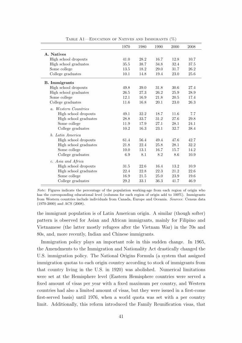
Table A1—Education of Natives and Immigrants (%)

1970 1980 1990 2000 2008

A. NativesHigh school dropouts 41.0 28.2 16.7 12.8 10.7High school graduates 35.5 38.7 34.8 32.4 37.5Some college 13.5 18.2 29.0 31.7 26.2College graduates 10.1 14.8 19.4 23.0 25.6

B. ImmigrantsHigh school dropouts 49.8 39.0 31.8 30.6 27.4High school graduates 26.5 27.3 26.2 25.9 28.9Some college 12.1 16.9 21.8 20.5 17.4College graduates 11.6 16.8 20.1 23.0 26.3

a. Western CountriesHigh school dropouts 49.1 32.2 18.7 11.6 7.7High school graduates 28.8 33.7 31.2 27.6 29.8Some college 11.9 17.9 27.1 28.1 24.1College graduates 10.2 16.3 23.1 32.7 38.4

b. Latin AmericaHigh school dropouts 61.4 56.4 49.4 47.6 42.7High school graduates 21.8 22.4 25.8 28.1 32.2Some college 10.0 13.1 16.7 15.7 14.2College graduates 6.9 8.1 8.2 8.6 10.9

c. Asia and AfricaHigh school dropouts 31.5 22.6 16.4 13.2 10.9High school graduates 22.4 22.8 22.3 21.2 22.6Some college 16.9 21.5 25.0 23.9 19.6College graduates 29.2 33.1 36.3 41.7 46.9

Note: Figures indicate the percentage of the population working-age from each region of origin whohas the corresponding educational level (columns for each region of origin add to 100%). Immigrantsfrom Western countries include individuals from Canada, Europe and Oceania. Sources: Census data(1970-2000) and ACS (2008).

the immigrant population is of Latin American origin. A similar (though softer)

pattern is observed for Asian and African immigrants, mainly for Filipino and

Vietnamese (the latter mostly refugees after the Vietnam War) in the 70s and

80s, and, more recently, Indian and Chinese immigrants.

Immigration policy plays an important role in this sudden change. In 1965,

the Amendments to the Immigration and Nationality Act drastically changed the

U.S. immigration policy. The National Origins Formula (a system that assigned

immigration quotas to each origin country according to stock of immigrants from

that country living in the U.S. in 1920) was abolished. Numerical limitations

were set at the Hemisphere level (Eastern Hemisphere countries were served a

fixed amount of visas per year with a fixed maximum per country, and Western

countries had also a limited amount of visas, but they were issued in a first-come

first-served basis) until 1976, when a world quota was set with a per country

limit. Additionally, this reform introduced the Family Reunification visas, that

41

Table A2—Share of Immigrants in each Occupation (%)

1970 1980 1990 2000 2008

A. Blue-collar 6.03 7.83 11.21 17.53 24.08Farm laborers 8.32 14.06 26.08 40.08 51.11Laborers 5.47 7.40 11.87 21.48 31.27Service workers 7.58 9.62 13.65 19.58 25.59Operatives 5.84 8.38 11.74 18.55 23.98Craftsmen 5.38 6.06 8.16 12.69 18.24

B. White-collar 4.96 5.76 7.70 10.78 13.34Professionals 6.29 6.90 8.64 11.95 14.50Managers 5.02 5.93 7.76 10.75 13.37Clerical and kindred 4.27 5.17 7.14 9.97 12.47Sales workers 4.78 5.03 6.78 9.29 11.52Farm managers 1.52 1.56 2.87 4.87 6.38

Note: Figures indicate the percentage of the workers employed in each occupation who are immigrants.Sources: Census data for 1970-2000 and ACS for 2008.

were granted in an unlimited number to immediate relatives (parents, spouses and

children) of U.S. citizens and legal immigrants. This policy change, as suggested

by Figure A1, switched radically the main sources of immigrants, motivating,

additionally, an important change in their skill composition.

Figure A1. Immigrants by National Origin (1875-2007)

00.03

0.06

0.09

0.12

0.15

1875 1890 1905 1920 1935 1950 1965 1980 1995 2010

Share of im

migrants

Year

Western Countries

Latin America

Asia and AfricaImmigration and

Nationality Act, 1965

Ratio

of immigrants over to

tal pop

ulation in each year

Note: The black solid line represents the share of the population working-age which is foreign born.The area below the dashed line corresponds to part of it that was born in Western Countries (Canada,Europe, and Oceania). The area between the dashed and the dotted lines corresponds to Latin Ameri-can immigrants. And the area between the dotted and the solid lines represents the share of Asian andAfrican immigrants. Sources: Census data (1870-2000) and ACS (2001-2008). Inter-Census interpola-tions based on the intensity of legal entry (Yearbook of Immigration Statistics 2009, U.S. Department ofHomeland Security) excluding the legalization of illegal immigrants granted with an amnesty by IRCA1986.

42

Appendix B: Model solution and estimation (detailed)


B1. A nested estimation algorithm

The equilibrium model presented in Section II does not have a closed form

solution and needs to be solved numerically. To explain the solution and esti-

mation algorithm, it is convenient to differentiate two types of parameters: ex-

pectation parameters, Θ2, which are given by the forecasting rules described in

equation (12), and the process for the aggregate shock (7), and fundamental pa-

rameters of the model, Θ1, which are the remaining parameters described in

Sections II.A and II.B. Forecasting rules are part of the solution of the model,

in the sense that their parameters ηjs are implicit functions of the fundamental

parameters. Parameters from the aggregate shock process are fundamental by

nature, but since the aggregate shock is estimated as a residual (i.e. an implicit

function of the data and fundamental parameters), and it is used to forecast future

skill prices in the same way forecasting rules given by equation (12) are used, I

treat (and estimate) them as expectation parameters. Hence, we can express Θ2

as Θ2(Θ1).

Parameters in Θ1 are estimated by Simulated Minimum Distance. The Simu-

lated Minimum Distance estimator minimizes the distance between a large num-

ber of statistics from the data (or data points) and their simulated counterparts.

Θ2(Θ1) is obtained as the fixed point of an algorithm that simulate the behavior

of individuals using a guess of Θ2, and then estimates equations (7) and (12) from

the simulated data to update the guess. Therefore, the estimator requires a nested

algorithm with a procedure that estimates Θ1, and another solving Θ2 given Θ1.

Lee and Wolpin (2006, 2010) describe a natural nested algorithm in which an

inner procedure finds the fixed point in Θ2 for every guess of Θ1, and an outer

loop solves the Θ1 estimation problem with a polytope algorithm. The main

drawback of this procedure is that it requires solving the fixed point problem in

every evaluation of Θ1, and this increases the computational burden significantly.36

I propose an alternative algorithm that avoids having to solve the fixed point in

every iteration of Θ1. In particular, I propose a swapping of the two procedures

which is in the same spirit of the swapping of conditional choice probabilities

and parameter estimation proposed by Aguirregabiria and Mira (2002). Θ1 is

36 This problem is relatively exacerbated if one uses the parallel version of the Simplex Methoddeveloped by Lee and Wiswall (2007) in the minimization problem. The basic idea in Lee andWiswall (2007) is to move the p worst parameters in each Simplex iteration. The problem isthat if one of the processors takes more iterations to find the fixed point in Θ2(Θ1) than allothers, the latter will remain idle while the former performs further iterations.

43

estimated for every guess of Θ2, which is updated at a lower frequency, i.e., I

estimate Θ1(Θ2) for every guess of Θ2. The algorithm consists of the following

steps:

1) Choose a set of parameters [Θ1]0 and [Θ2]0.37

2) Solve the optimization problem for each cohort that exists from t = 1 to t =

T .38 This dynamic programming problem (given by equation (1)) is solved

recursively by backwards induction from age 65 to age 16. This solution

is not analytic. Moreover, the size of the state space is infinite, and even

discretizing the continuous variables with a relatively small number of grid

points, it still remains impossible to handle. As introduced by Keane and

Wolpin (1994, 1997), in each period I solve the problem for a subset of the

state space and then I estimate an interpolation rule as a function of the state

variables.39 Unlike in these papers and in Lee and Wolpin (2006, 2010), I

use a gaussian quadrature instead of Monte Carlo integration to numerically

compute the multiple-dimensional integrals from the expectation of the value

function in t+ 1.40

3) Find the skill rental prices that clear the market and the aggregate shock

that closes the production function simulating the economy from t = 1 to

t = T . More specifically,

a) Guess skill rental prices of period t = 1.

b) Find the supply of skills at this price using the solution of the individual

optimization problem obtained in step 2.

37 A very natural initial guess for Θ2 is given by the solution of the fixed point algorithmdescribed in step 5 given [Θ1]0.

38 I assume that the economy begins in 1860. This very early initial date is so to overcomethe arbitrary initial conditions that I assign to all cohorts existing in t = 1. In 1967, the firstestimation year, slightly more than two entire generations have gone by. Hence, the oldestindividuals (the ones turning 65 that year) have never coexisted in the model with any of theinitial cohorts. T is the last estimation year, which is 2007; the youngest individuals that are inthe model that year will die in 2057.

39 The model is solved at 1,280,000 different points of the state space. For each of this points,the expected value function at the selected alternative —known in the literature as the Emaxfunction— is obtained. Then, the interpolation rule is estimated as a set of regressions of thelog Emax on education, a quadratic in blue collar and white collar experienced the interactionof education, blue collar experience, and white collar experience, predicted skill prices usingequation (12), interactions of these predicted skill prices with education, blue collar experience,and white collar experience, a time trend, number of children, and foreign potential experience.These eighteen regression coefficients are estimated for every age, individual type, and for each ofthe four alternatives chosen potentially chosen in the preceding period. Hence, the interpolationrule that delivers the Emax at every potential point of the state space consists of 28,224 regressioncoefficients.

40 Although being more time consuming, gaussian quadrature is known to be widely moreaccurate than Monte Carlo integration.

44

c) Plug the supply of skills into the production function and, together with

data on capital and output, recover the aggregate shock as a residual.

d) Update skill rental prices with the demand equations (9) and (10),

using the supply of labor obtained in step 3b and the aggregate shock

from step 3c.

e) Repeat steps 3b to 3d using the prices obtained in 3d as the updated

guess. Keep iterating to find a fixed point in skill prices. These are

the skill prices that clear the market, since they equalize supply and

demand.

f) Repeat steps 3b to 3e for t = 2, ..., T .

4) Compare the statistics computed with simulated data and their observed

counterparts. Update Θ1 with a simplex iteration and repeat steps 2 and 3

with [Θ1]1. Keep updating Θ1 till finding the set of parameters that minimize

the distance between simulated and observed data, Θ1([Θ2]0).

5) Given Θ1([Θ2]0), update [Θ2]1 = Θ2(Θ1([Θ2]0)). In particular, fit OLS re-

gressions of equations (7) and (12) with the simulated aggregate data ob-

tained at the end of step 3. Iterate solving steps 2 and 3 using these OLS

estimates to compute expectations until reaching the fixed point.41

6) If [Θ2]1 = [Θ2]0, the algorithm finishes. Otherwise, repeat steps 2 to 5 with

the updated guesses [Θ2]1 and Θ1([Θ2]0) until convergence is reached.

B2. Data and estimation

The Simulated Minimum Distance estimator minimizes a weighted average squared

distance between a large set of statistics from the data or data points, and their

simulated counterparts.42 Table B1 lists the set of statistics I use in the esti-

mation. Each statistic is weighted by the inverse of the sample size used in its

calculation (see further details in Appendix E).

The model is fitted to annual data from 1967 to 2007. The annual frequency

introduces the problem that individuals may not spend the full year doing the

same activity. Therefore, in order to assign individuals to one of the four mutually

exclusive alternatives, I apply the following rules:

41 This step does not necessarily need to be done after reaching a convergence in Θ1 given[Θ2]0. Periodic updates of expectation parameters can also be programmed after K iterations.Indeed, if K = 1, this algorithm coincides with the one described in Lee and Wolpin (2006,2010).

42 They are data points in the same sense that a cohort observed at a point in time is anindividual observation in a cohort analysis, or the labor supply in an education-experience cellis an observation in Borjas (2003) regressions.

45

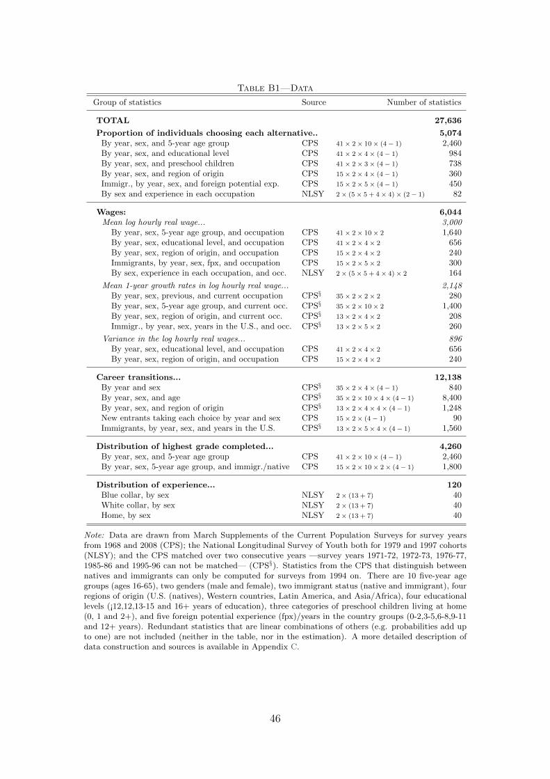
Table B1—Data

Group of statistics Source Number of statistics

TOTAL 27,636

Proportion of individuals choosing each alternative.. 5,074By year, sex, and 5-year age group CPS 41× 2× 10× (4− 1) 2,460By year, sex, and educational level CPS 41× 2× 4× (4− 1) 984By year, sex, and preschool children CPS 41× 2× 3× (4− 1) 738By year, sex, and region of origin CPS 15× 2× 4× (4− 1) 360Immigr., by year, sex, and foreign potential exp. CPS 15× 2× 5× (4− 1) 450By sex and experience in each occupation NLSY 2× (5× 5 + 4× 4)× (2− 1) 82

Wages: 6,044Mean log hourly real wage... 3,000

By year, sex, 5-year age group, and occupation CPS 41× 2× 10× 2 1,640By year, sex, educational level, and occupation CPS 41× 2× 4× 2 656By year, sex, region of origin, and occupation CPS 15× 2× 4× 2 240Immigrants, by year, sex, fpx, and occupation CPS 15× 2× 5× 2 300By sex, experience in each occupation, and occ. NLSY 2× (5× 5 + 4× 4)× 2 164

Mean 1-year growth rates in log hourly real wage... 2,148By year, sex, previous, and current occupation CPS§ 35× 2× 2× 2 280By year, sex, 5-year age group, and current occ. CPS§ 35× 2× 10× 2 1,400By year, sex, region of origin, and current occ. CPS§ 13× 2× 4× 2 208Immigr., by year, sex, years in the U.S., and occ. CPS§ 13× 2× 5× 2 260

Variance in the log hourly real wages... 896By year, sex, educational level, and occupation CPS 41× 2× 4× 2 656By year, sex, region of origin, and occupation CPS 15× 2× 4× 2 240

Career transitions... 12,138By year and sex CPS§ 35× 2× 4× (4− 1) 840By year, sex, and age CPS§ 35× 2× 10× 4× (4− 1) 8,400By year, sex, and region of origin CPS§ 13× 2× 4× 4× (4− 1) 1,248New entrants taking each choice by year and sex CPS 15× 2× (4− 1) 90Immigrants, by year, sex, and years in the U.S. CPS§ 13× 2× 5× 4× (4− 1) 1,560

Distribution of highest grade completed... 4,260By year, sex, and 5-year age group CPS 41× 2× 10× (4− 1) 2,460By year, sex, 5-year age group, and immigr./native CPS 15× 2× 10× 2× (4− 1) 1,800

Distribution of experience... 120Blue collar, by sex NLSY 2× (13 + 7) 40White collar, by sex NLSY 2× (13 + 7) 40Home, by sex NLSY 2× (13 + 7) 40

Note: Data are drawn from March Supplements of the Current Population Surveys for survey yearsfrom 1968 and 2008 (CPS); the National Longitudinal Survey of Youth both for 1979 and 1997 cohorts(NLSY); and the CPS matched over two consecutive years —survey years 1971-72, 1972-73, 1976-77,1985-86 and 1995-96 can not be matched— (CPS§). Statistics from the CPS that distinguish betweennatives and immigrants can only be computed for surveys from 1994 on. There are 10 five-year agegroups (ages 16-65), two genders (male and female), two immigrant status (native and immigrant), fourregions of origin (U.S. (natives), Western countries, Latin America, and Asia/Africa), four educationallevels (¡12,12,13-15 and 16+ years of education), three categories of preschool children living at home(0, 1 and 2+), and five foreign potential experience (fpx)/years in the country groups (0-2,3-5,6-8,9-11and 12+ years). Redundant statistics that are linear combinations of others (e.g. probabilities add upto one) are not included (neither in the table, nor in the estimation). A more detailed description ofdata construction and sources is available in Appendix C.

46

i. An individual is assigned to school if she reported that school was her main

activity during the survey week (CPS) or if she was attending school at

survey date (NLSY).

ii. She is assigned to work in one of the two occupations if she is not assigned to

school, and she worked at least 40 weeks during the previous year and at least

20 hours per week. When an individual is assigned to work, her occupation

is the one held during the last year (CPS) or the most recent one (NLSY).

Craftsmen, operatives, service workers, laborers, and farmers are classified

as blue collar workers, whereas professionals, clerks, sales workers, managers

and farm managers are white collar workers.

iii. Individuals that are neither assigned to attend school nor to work are con-

sidered to stay at home.

The simulated counterparts of the statistics described in Table B1 are obtained

by simulating the behavior of cohorts of 2,000 natives and 3,000 immigrants (some

of them starting their life abroad and not making decisions until they enter the

U.S.). Therefore, cross-sectional simulated data are calculated with a sample of

up to 250,000 observations, which are weighted using data on cohort sizes.

The solution of the model requires additional data for exogenous aggregate

variables: output, stock of equipment capital and structures, cohort sizes (by

gender and immigrant status), the distribution of entry age for immigrants, the

distribution of initial schooling (at age 16 for natives and upon entry in the U.S. for

immigrants), the distribution of immigrants by region of origin, and the fertility

(preschool children) process. The sources, definitions, and construction of all these

variables are detailed in Appendix C.

Identification of the parameters of the model requires that there is no parameter

vector that is “observationally equivalent” to the true parameter vector. Under

correct specification of the model, the true parameter vector makes the differ-

ence between the population statistics and the counterparts generated by the

model (when the number of simulated individuals tends to infinity) equal to zero.

The identification condition requires that there is no other parameter vector that

achieves this value. Unfortunately, there is no formal proof of whether this condi-

tion is satisfied for the set of statistics listed in Table B1. It is a matter of unique-

ness of the global minimum and curvature around it. Heuristically, I present an

informal check of the latter in Figure D1 in Appendix D. This figure plots different

sections of the objective function in which I move one parameter and keep the

others constant to the estimated values. Although this exercise is uninformative

about the curvature in the multidimensional space, it shows plenty of unilateral

curvature for all parameters. Pointing in the same line, standard errors of the

47

estimates reported below are very small, which is significant because they depend

on the curvature of the objective function around parameter estimates —see Ap-

pendix E. Regarding uniqueness, the only robustness that can be performed is to

start the estimation from different initial conditions and keep the local minimum

that gives a smaller value for the objective function.

Despite not being able to formally prove identification, we can have an intuition

on what is the variation that identifies the parameters with the used data. Identi-

fication would be achieved by a combination of functional forms and distributional

assumptions, along with exclusion restrictions. The present analysis is not very

different in spirit from the synthetic cohort panel data analysis used, for example,

in Browning, Deaton and Irish (1985) (indeed, a large fraction of the data listed in

Table B1 are cohort specific). Exclusion restrictions to identify wage equations are

provided by variables that affect utilities and not wages (e.g. preschool children),

and, for utility functions, they are given by variables that are in wage equations

and not in utility functions (e.g. experience). Production function parameters are

identified by functional form assumptions from the aggregate supply of skill units

plus aggregate data on capital and output; current and past cohort sizes act as

instruments for skill units.

48

Appendix C: Variable definitions and sources


Both the solution and the estimation of the model combine a variety of aggregate

and micro-level data. In this Appendix, I describe the construction of the variables

and the data sources.

C1. Aggregate data

Aggregate macro data are used in the solution of the model, as described in

the main text. The estimation period is 1967-2007. However, in order to vanish

initial conditions, I simulate the model starting in 1860. The model is initialized

by simulating the first 40 years (1860-1900) using aggregate data for 1900. Then

I simulate the remaining years (1900-2007) with actual macro data. As a result,

two entire generations go by before the first year of estimation.

Output. Output is measured as Gross Domestic Product at chain 2000 U.S.

dollars, provided by the Bureau of Economic Analysis (BEA), NIPA Table 1.1.6.

Given that the original series starts in 1929, I use the average annual growth rate

(1929-2007) to extrapolate backwards to year 1900.

Capital stock. There are two types of capital in the model: structures and

equipment capital. Both series are extracted from BEA, combining flow data

from Fixed Assets Tables 1.2 (“Chain-Type Quantity Indexes for Net Stock of

Fixed Assets”) with year 2000 stock data from Fixed Assets Table 1.1 (“Current

Cost Net Stock of Fixed Assets”). Resulting series are expressed in chain 2000

U.S. dollars. Series start in 1925, so I extrapolate them backwards to 1900 using

average annual growth rates.

Cohort sizes. Cohort sizes are extracted from Integrated Public Use Microdata

Series (IPUMS) of the U.S. Census.43 In particular, I use information from the de-

cennial Censuses from 1900 to 2000, and from the American Community Survey

(ACS) 2001-2007. A person is classified as an immigrant if born abroad; indi-

viduals born in Puerto Rico and other outlying areas are categorized as natives.

Native and immigrant inter-census cohort sizes are estimated following different

procedures. For natives, I distributing the cumulative decade cohort size decrease

to each year using annual data on mortality rates by age from Vital Statistics of

the U.S. (National Center for Health Statistics). For immigrants, I use a simi-

lar procedure, using the estimates of the entry age distribution described below

instead of mortality rates.

43 Ruggles, Sobek, Alexander, Fitch, Goeken, Hall, King and Ronnander (2008).

49

Age at entry. The distribution of entry age of immigrants is estimated using

U.S. Census IPUMS. In order to reduce small sample noise, I average out the

distributions for immigrants who arrived at t− 1, t− 2,..., t− 5. Since the exact

year of immigration is only available in 1900-1930 and 2000 Censuses, and in the

ACS (2001-2007), intermediate years are linearly interpolated. Given that the

distribution is stable over the years, I estimate a single distribution for each of the

following intervals: 1900-1930, 1931-1940, 1941-1950, 1951-1960, 1961-1970, 1971-

1980, 1981-1990 and 1991-2007. Finally, in order to obtain the joint distribution of

age at entry and initial education, I estimate the entry age distribution conditional

on education. Because of data limitations, I approximate it using the “relative”

distribution by educational level, i.e. I compute the ratio of conditional and

unconditional distributions from the Census 2000, and then I multiply this relative

distribution with the time varying unconditional age at entry distribution.44

Regions of origin. I consider three regions of origin for immigrants: Western

Countries, Latin America, and Asia-Africa. Western Countries include Europe,

Canada and Atlantic Islands, and Oceania; Latin America include Caribbean

Countries, Mexico, and Central and South America; Asia-Africa includes all im-

migrants from these two continents. The stock of immigrants from each of these

regions are drawn from U.S. Census IPUMS 1900-2000 and ACS 2001-2007. Inter-

census estimates of the stock of immigrants from each region of origin are obtained

by combining a linear interpolation of the share of immigrants from each region

and the estimated of cohort sizes described above. The share of the total inflow

of immigrants in year t that comes from region i, sflowi,t , is then estimated as:

sflowi,t =Mtsi,t −Mt−1si,t−1 + s65,i,t−1M65,t−1

Mt −Mt−1 +M65,t−1

, (C1)

where Mt is the stock of immigrants in year t, si,t is the share of immigrants

that are natural from region i in period t, and M65,t is the stock of 65 years old

immigrants in year t. The share s65,i,t−1 is approximated with si,t−35 because the

average age at entry is around 30 years. The numerator of equation (C1) is the

flow of immigrants from region i in period t, i.e. the observed increase in the stock

plus the recovery of those who died (reached age 65); the denominator is the total

inflow in period t.

Initial education. Immigrants and natives are assigned initial years or educa-

tion differently. Initial education of natives is allocated at age 16. The distribution

of years of education at this age (by gender) is estimated using U.S. Census IPUMS

44 This calculation assumes that the relative distribution is constant over time. Estimatesusing 1970-1990 Censuses (for which the year of entry is only available by five-year intervals)support this assumption.

50

for 1940-2000 and ACS 2001-2007. Inter-census estimates are linearly interpo-

lated. In censuses before 1940 there is no information on education. Therefore, I

use the 1940 Census to infer the initial education of cohorts aged 16 in each of the

previous census years, assuming that they concentrate education at the beginning

of their lives, and that mortality at these ages is small enough so that it does not

induce any bias. Immigrants are assigned education when they enter the United

States. To this end, I use U.S. Census IPUMS for years 1970-2000. I assume that

immigrants also concentrate their education spells at the beginning of their life;

therefore, an individual with a college degree that enters at age 40 is assumed to

enter with the college degree, whereas another that entered at age 18 is assumed

to enter with a high school diploma.45 To impute education to earlier cohorts of

immigrants, I estimate the distribution of years of education by cohort of entry

using U.S. Census of 1970.

Fertility process. The fertility process is given by the transition probability

matrix from 0, 1, or 2+ preschool children at home in period t into 0, 1 or 2+

in t + 1, conditional on age, education, and gender. Data are drawn from CPS

1964-2007 and U.S. Census 1900-1960. Before 1960, the transition probability

matrix is not conditional on education.

Wage adjustments. To avoid biases in parameter estimates, I make three ad-

justments to wages and/or aggregate skill units. On the one hand, both CPS

wages and output data include taxes, but individuals make decisions on a net

income basis; to correct for this, I simulate individuals’ decisions using net wages,

deflating gross simulated wages (fitted to the data) by the ratio of Disposable Per-

sonal Income over Personal Income (Bureau of Economic Analysis, NIPA Table

2.1). On the other hand, there are two reasons why total labor compensation pro-

duced by the model could be underestimated without further adjustments (and

factor shares, biased as a result): first, the focus on intensive margin, and the

use of the year as the time unit, generates some discrepancies between aggre-

gated earnings simulated from the model and actual aggregate earnings (some

individuals that work a small fraction of the year are considered as not working,

whereas others that work a large fraction of the year, but not the entire period,

are assumed to work full time for the whole year); and, second, there are some

forms of labor compensation that are not wages (e.g. some types of bonuses

and in-kind payments). These two discrepancies are corrected by adjusting total

wage compensation appropriately. To correct for the first, I adjust the aggregate

simulated wage compensation by the ratio of BEA Total Wage and Salary Dis-

45 This assumption is supported by the human capital investment literature (e.g. Becker,1964).

51

bursements (NIPA Table 2.1) over the aggregation of wages obtained from the

CPS. The second concern is addressed using the ratio of BEA Total Wage and

Salary Disbursements over the Total Compensation of Employees (NIPA Table

2.1).

C2. Microdata

All micro-data statistics used in the estimation (and listed in Table B1) are

constructed with data from two different sources: March Supplement of Current

Population Survey (CPS), and the two cohorts (1979 and 1997) from the National

Longitudinal Survey of Youth (NLSY).46

Age groups. Individuals are grouped in ten 5-year age groups from 16-20 years

old to 61-65. Individuals above 65 and below 16 are not in the model and they

are dropped from the samples.

Educational level. I categorize individuals in four education groups: high school

dropouts (¡12 years of education), high school graduates (12), persons with some

college (13-15), and college graduates (16+). In 1992, a methodological change

was introduced to CPS regarding education. Before that year, the education vari-

able gives the respondent’s highest grade of school or year of college completed;

beginning in 1992, the variable classifies high school graduates according to their

highest degree or diploma attained. I use the IPUMS recoded educational attain-

ment variable to make it comparable over the years.

Experience. Years of effective experience in blue collar and white collar occu-

pations are calculated from NLSY. The samples are restricted to individuals born

from 1962 to 1964 for NLSY79 and from 1980 to 1984 for the NLSY97. I consider

only individuals for which their entire path of choices from age 18 to either 1993,

1992, 1991 or 1990 for NLSY79 or to 2006, 2005 or 2004 for NLSY97 is observable.

Individual choices are assigned as described below. Experience is counted as the

number of years that the individual’s choice was to work in the corresponding

occupation.

46 CPS data are extracted from IPUMS (Ruggles et al., 2008). The CPS interviews householdsfor 8 eight months; more concretely, when a household enters the sample for the first time isinterviewed four consecutive months, then not interviewed during eight months, and finallyinterviewed four additional consecutive months (which are the same four calendar months fromthe first spell, but in the subsequent year). Therefore, a household that is in the March sampleis interviewed in March for two consecutive years. As a result, in most of the survey years, itis possible to match a subset of households for two consecutive years obtaining a small panel.IPUMS data has a recoded individual and household identifier that does not allow to matchconsecutive surveys, and for this reason, I use samples extracted from the NBER to do thematching. Survey years 1971-72, 1972-73, 1976-77, 1985-86 and 1995-96 can not be matcheddue to survey changes.

52

Choices. Individuals are assigned to one of the four mutually exclusive year

round alternatives: blue collar or white collar work, attend school, or stay at home.

The procedure to assign individuals follows a hierarchical rule. An individual is

assigned to school if she reported that school was her main activity during de

survey week (CPS) or if she was attending school at survey date (NLSY). She is

assigned to work in either of the two occupations if she is not assigned to school

and she worked at least 40 weeks during the year before the survey date, and

at least 20 hours per week.47 When an individual is assigned to work, she is

assigned to the occupation held during the last year (CPS) or the most recent

(NLSY). Blue collar occupations include craftsmen, operatives, service workers,

laborers, and farmers, and white collar include professionals, clerks, sales workers,

managers, and farm managerial occupations. Finally, those individuals that are

not assigned neither to work nor to attend school are assigned to stay at home.

Wages. Hourly wage is computed for individuals that are assigned to either of

the work alternatives according to the previous definition. Workers are assumed to

earn their wage entirely in the occupation they are assigned to. Earnings include

wage and salary income, and self-employment earnings, deflated to year 2000 U.S.$

using the Consumer Price Index. Top-coded annual earnings are multiplied by 1.4;

extreme observations are dropped (hourly real wage lower than $2 or larger than

$200).48 Hours worked are calculated combining information on weeks worked last

year and hours worked last week.49 50

Preschool children. Individuals are allowed to have 0,1, or 2+ preschool chil-

dren (less than five years old). In the data, households are defined as family units;

preschool children living in a two family home are only assigned to their parents.

In order to link children with their parents, I use IPUMS-created variables momloc

and poploc, which identify the position of the mother and father in the household

respectively. Parent definition includes biological, step- and adoptive parents. Al-

though they fully comparable over years, there are some minor changes that are

listed in the database documentation.

47 Hours per week are approximated by the number of hours worked in the previous week.48 This approach is followed, for instance, by Lemieux (2006).49 Before 1976, weeks worked last year are only available by intervals; in particular, the

relevant intervals are 40-47, 48-49 and 50-52 weeks. Each interval is imputed, respectively 43.1,48.3 and 51.9 weeks. These figures are obtained from sample means for each interval using datafor the five years after 1975.

50 In the model, individuals are assumed to work 2080 hours per year (40 hours, 52 weeks).Although hours worked by individuals assigned to working categories average a little above thisquantity, there is an important concentration of workers in the amount of 40 hours per week(Keane and Moffitt, 1998).

53

Region of origin. The region of birth is assigned as described above for the

aggregate data. A small number of individuals for which the country of birth

is unknown are dropped from the corresponding samples. CPS started to ask

questions related to immigrant status in survey year 1994. Therefore, statistics

that include this information are only used from that survey date onwards.

Potential experience abroad. The initial experience endowment for immi-

grants (experience obtained abroad) is measured as “potential experience” given

data availability. In particular, this variable is defined as age at entry minus years

of education, minus 6. In the CPS, year of immigration is only available by in-

tervals; additionally, education is also grouped in 0-4, 5-8, 9, 10, 11, 12, 13-15

and 16+ years of education intervals. To construct experience abroad, I use the

central point of the corresponding interval both for age at entry and for years of

education. Since I do not observe where did the education take place, I assume

that individuals concentrate their education spells in the beginning of their lives,

regardless of the country in which they were living. Therefore, if an individual’s

age at entry minus completed education (and minus 6) is zero or negative, I as-

sume that the individual entered in the U.S. with zero experience. The resulting

variable is then grouped into the following categories: 0-2, 3-5, 6-8, 9-11 and 12+

years.

Years in the U.S. This variable is constructed in an analogous way to potential

experience abroad. It is also grouped in the same categories.

54

Appendix D: Curvature of the objective function


Figure D1. Sections of the objective function

50

50.6

51.2

51.8

52.4

53

53.6

54.2

54.8

0.49 0.53 0.57 0.61

α

50

50.6

51.2

51.8

52.4

53

53.6

54.2

54.8

0.37 0.42 0.47 0.52

θ

50

50.6

51.2

51.8

52.4

53

53.6

54.2

54.8

0.24 0.27 0.3 0.33

ρ

50

50.5

51

51.5

52

52.5

53

53.5

54

-0.13 -0.09 -0.05 -0.01

γ

50

50.5

51

51.5

52

52.5

53

53.5

54

0.01 0.07 0.13 0.19

λ

50

50.4

50.8

51.2

51.6

52

52.4

52.8

53.2

11400 12200 13000 13800

τ1

50

50.3

50.6

50.9

51.2

51.5

51.8

52.1

52.4

7000 16000 25000 34000

τ2

50

50.4

50.8

51.2

51.6

52

52.4

52.8

53.2

-0.18 0 0.18 0.36

ωB0,West

50

50.6

51.2

51.8

52.4

53

53.6

54.2

54.8

-0.14 -0.02 0.1 0.22

ωB0,Lat

50

50.4

50.8

51.2

51.6

52

52.4

52.8

53.2

-0.27 -0.09 0.09 0.27

ωB0,As-Af

50

50.8

51.6

52.4

53.2

54

54.8

55.6

56.4

-0.3465 -0.3415 -0.3365 -0.3315

ωB0,Female

50

50.5

51

51.5

52

52.5

53

53.5

54

-0.18 0.03 0.24 0.45

ωW0,West

50

50.6

51.2

51.8

52.4

53

53.6

54.2

54.8

-0.34 -0.22 -0.1 0.02

ωW0,Lat

50

50.6

51.2

51.8

52.4

53

53.6

54.2

54.8

-0.22 -0.04 0.14 0.32

ωW0,As-Af

50

50.8

51.6

52.4

53.2

54

54.8

55.6

56.4

-0.304 -0.297 -0.29 -0.283

ωW0,Female

50

50.15

50.3

50.45

50.6

50.75

50.9

51.05

51.2

1800 2200 2600 3000

δS0,Male

50

50.3

50.6

50.9

51.2

51.5

51.8

52.1

52.4

-16000 0 16000 32000

δS0,West

50

50.3

50.6

50.9

51.2

51.5

51.8

52.1

52.4

0 2000 4000 6000

δS0,Lat

50

50.4

50.8

51.2

51.6

52

52.4

52.8

53.2

-8000 4000 16000 28000

δS0,As-Af

50

50.5

51

51.5

52

52.5

53

53.5

54

5000 5400 5800 6200

δS0,Female

50.1

50.4

50.7

51

51.3

51.6

51.9

52.2

52.5

16000 16400 16800 17200

δH0,Male

50.1

50.4

50.7

51

51.3

51.6

51.9

52.2

52.5

9000 14000 19000 24000

δH0,West

50

50.6

51.2

51.8

52.4

53

53.6

54.2

54.8

9000 11000 13000 15000

δH0,Lat

50

50.4

50.8

51.2

51.6

52

52.4

52.8

53.2

9000 13000 17000 21000

δH0,As-Af

50

50.6

51.2

51.8

52.4

53

53.6

54.2

54.8

11100 11250 11400 11550

δH0,Female

49.8

50.2

50.6

51

51.4

51.8

52.2

52.6

53

0.07225 0.07275 0.07325 0.07375

ωB1,Nat

50

50.6

51.2

51.8

52.4

53

53.6

54.2

54.8

0.049 0.055 0.061 0.067

ωB1,Imm

50

50.4

50.8

51.2

51.6

52

52.4

52.8

53.2

0.0929 0.0933 0.0937 0.0941

ωB2,B

50

50.4

50.8

51.2

51.6

52

52.4

52.8

53.2

0.028 0.0288 0.0296 0.0304

ωB2,W

50

50.5

51

51.5

52

52.5

53

53.5

54

-0.002365 -0.00234 -0.002315 -0.00229

ωB3,B

50

50.3

50.6

50.9

51.2

51.5

51.8

52.1

52.4

-0.00139 -0.00134 -0.00129 -0.00124

ωB3,W

50

50.5

51

51.5

52

52.5

53

53.5

54

0.007 0.014 0.021 0.028

ωBF

50

50.3

50.6

50.9

51.2

51.5

51.8

52.1

52.4

0.1087 0.1094 0.1101 0.1108

ωW1,Nat

50

50.5

51

51.5

52

52.5

53

53.5

54

0.101 0.107 0.113 0.119

ωW1,Imm

50

50.4

50.8

51.2

51.6

52

52.4

52.8

53.2

0 0.001 0.002 0.003

ωW2,B

50

50.15

50.3

50.45

50.6

50.75

50.9

51.05

51.2

0.1046 0.1052 0.1058 0.1064

ωW2,W

50

50.5

51

51.5

52

52.5

53

53.5

54

-0.0007 -0.00055 -0.0004 -0.00025

ωW3,B

50.1

50.4

50.7

51

51.3

51.6

51.9

52.2

52.5

-0.00298 -0.00292 -0.00286 -0.0028

ωW3,W

50.1

50.3

50.5

50.7

50.9

51.1

51.3

51.5

51.7

-0.074 -0.056 -0.038 -0.02

ωWF

50

50.5

51

51.5

52

52.5

53

53.5

54

7950 8650 9350 10050

δBW1,Male

50

50.8

51.6

52.4

53.2

54

54.8

55.6

56.4

10400 11700 13000 14300

δBW1,Female

50

50.6

51.2

51.8

52.4

53

53.6

54.2

54.8

26400 29400 32400 35400

δS1,Male

50

50.5

51

51.5

52

52.5

53

53.5

54

26800 30800 34800 38800

δS1,Female

49.9

50

50.1

50.2

50.3

50.4

50.5

50.6

50.7

50.8

-2100 -1900 -1700 -1500

δH1,Male

50

50.6

51.2

51.8

52.4

53

53.6

54.2

54.8

3100 3500 3900 4300

δH1,Female

50

50.3

50.6

50.9

51.2

51.5

51.8

52.1

52.4

48.5 53.5 58.5 63.5

δH2,Male

50

50.6

51.2

51.8

52.4

53

53.6

54.2

54.8

48 51 54 57

δH2,Female

50

50.15

50.3

50.45

50.6

50.75

50.9

51.05

51.2

0.375 0.415 0.455 0.495

σB1,Male

50

50.3

50.6

50.9

51.2

51.5

51.8

52.1

52.4

0.495 0.525 0.555 0.585

σW1,Male

50

50.2

50.4

50.6

50.8

51

51.2

51.4

51.6

600 1200 1800 2400

σS1,Male

50

50.6

51.2

51.8

52.4

53

53.6

54.2

54.8

10000 10300 10600 10900

σH1,Male

50

50.8

51.6

52.4

53.2

54

54.8

55.6

56.4

0.32 0.37 0.42 0.47

σB1,Female

50

50.3

50.6

50.9

51.2

51.5

51.8

52.1

52.4

0.445 0.475 0.505 0.535

σW1,Female

50

50.4

50.8

51.2

51.6

52

52.4

52.8

53.2

0 1000 2000 3000

σS1,Female

50

50.4

50.8

51.2

51.6

52

52.4

52.8

53.2

4200 4800 5400 6000

σH1,Female

50

50.4

50.8

51.2

51.6

52

52.4

52.8

53.2

0.041 0.059 0.077 0.095

ρBW

Note.— Solid lines plot the evolution of the objective function when changing the correspondingparameter and leaving others constant at the estimated values. Red dots indicate parameterpoint estimates.

55

Appendix E: Standard errors


Parameter estimates are the result of the following minimum distance estimation

problem:

θ = arg minθ||π(x)− π(xS(θ))|| =

= arg minθ

[π(x)− π(xS(θ))]′W [π(x)− π(xS(θ))]. (E1)

Weights are proportional to the sample size used to calculate each statistic. In

particular, I consider a diagonal matrix with the (weighted) sample size of each

element.51

The asymptotic distribution of parameters is obtained by applying the delta

method to the sample statistics. In particular,

V ar(θ) = (G′WG)−1G′WV0WG(G′WG)−1, (E2)

where G is the P ×R matrix of partial derivatives of the R statistics included in

π with respect to the P parameters included in θ.

In the estimation problem defined by equation (E1) there are two sources of

error. First, data statistics π(x) are estimated with sampling error. And second,

the function that maps parameters into statistics, π(xS(θ)), does not have a closed

form solution, and I need to simulate it, introducing a simulation error.

The remainder of this Appendix is devoted to provide an estimator of V0. It

is important to notice that, given the two sources of error, asymptotic theory

should be applied two-way: taking the sample size and the number of simulations

to infinity. To handle it, the problem can be split in the difference between the

following two elements:√N (π(x)− π(θ0)) and

√M (π(xS(θ0))− π(θ0)), where

N is the sample size and M is the number of simulations.

E1. Minimum distance asymptotic results

Consider R statistics from the data such that:

E[YK ] = πk(θ0), k = 1, ..., R. (E3)

We are assuming that those statistics are means, but this can be done without a

loss of generality. Those means are estimated with k different samples Sk, each of

51 Weighted sample size is defined in this context as(∑

i p2i / (∑

i pi)2)−1

, where pi is the

individual weight in the sample. If pi = p ∀i, this sum is equal to the sample size. Theweighted sample size is inverse of the precision of the variance of the weighted sample mean:V ar(x) = σ2

x

∑i p

2i / (∑

i pi)2.

56

them of size Nk. Notice that some of these samples may overlap (e.g., the sample

used to estimate the share of 16-20 years old males choosing to work in blue collar

in year 1967 may include some individuals that are also used to estimate the

share of high school dropout males choosing blue collar in that year). Sample

counterparts of these statistics are given by

πk =1

Nk

∑i∈Sk Yki. (E4)

Therefore, if the functional form of π(θ) was known, we could write

θ = arg minθ∈Θ||π − π(θ)||. (E5)

Let us introduce some additional notation:

dki ≡ 1i ∈ Sk, (E6)

Sij ≡ Si ∩ Sj, (E7)

S ≡ S1 ∪ ... ∪ SR, (E8)

N ≡∑

i∈S

(∑k dki −

∑k

∑j dkidji

), (E9)

λkN ≡Nk

N

N→∞−−−→ λk, (E10)

ψki ≡ Yki − πk(θ0). (E11)

Now we can write√N1(π1 − π1)√N2(π2 − π2)

...√NR(πR − πR)

=

1√N1

∑i∈S1

ψ1i

1√N2

∑i∈S2

ψ2i

...1√NR

∑i∈SR ψRi

=

√λ1N 0 . . . 0

0√λ2N . . . 0

......

. . ....

0 0 . . .√λRN

−1

×

× 1√N

∑i∈S

d1iψ1i

d2iψ2i

...

dRiψRi

≡ Λ 1√N

∑i∈S di ψi, (E12)

where denotes the Hadamard or element-by-element product. Due to the central

limit theorem (CLT), and Cramer’s theorem, as N →∞:

Λ1√N

∑i∈S di ψi→

dN (0,ΛE[(di ψi)(ψi di)′]Λ) . (E13)

57

Therefore, by the analogy principle we can define an estimator of the variance-

covariance matrix of the R sample statistics as

Ω =

1N1σ2

1N12

N1N2σ12 . . . N1R

N1NRσ1R

N12

N1N2σ12

1N2σ2

2 . . . N2R

N2NRσ12

......

. . ....

N1R

N1NRσ1R

N2R

N2NRσ2R . . . 1

NRσ2R

(E14)

where σij = 1Nij

∑k∈Sij ψkiψ

′kj, and σ2

i = 1Ni

∑k∈Si ψkiψ

′ki.

E2. Simulated minimum distance asymptotic results

Suppose that π is an estimator of some characteristic π of the distribution of Y

based on the sample YiNi=1 such that

√N [π − π(θ0)]→

dN (0,Ω). (E15)

Let us assume that for known functions g(., .) and F (.),

Y = g(U, θ0) U ∼ F. (E16)

Let π(θ0, UM) represent the same estimating formula as π but based on the artifi-

cial sample g(Uj, θ0)Mj=1 constructed from a simulated sample UM . As M →∞we have √

M [π(θ0, UM)− π(θ0)]→

dN (0,Ω) (E17)

independently of π. Therefore, as long as 0 < limN,M→∞(N/M) ≡ κ <∞√N [π − π(θ0, U

M)] =

=√N [π − π(θ0)]−

√N

M

√M [π(θ0, U

M)− π(θ0)]→dN (0, (1 + κ) Ω) (E18)

Note that this result includes the case in which we can simulate a sample of size

m for every observation i = 1, ..., N , so that M = mN , and κ = 1/M , which is

the case analyzed in McFadden (1989).

Finally, to generalize the result to multiple statistics with overlapping samples

as in Section E1, let (l1i, ..., lRi) and (δ1, ..., δR) play the role of (d1i, ..., dRi) and

(λ1, ..., λR) in the simulated samples, we similarly have that√M1(π1(θ0, U

M1)− π1)√M2(π2(θ0, U

M2)− π2)

...√MR(πR(θ0, U

MR)− πR)

≡ ∆1√M

∑i∈UM liψi→

dN (0,∆E[(li ψi)(ψi li)′]∆) .

(E19)

58

Therefore, √N1(π1 − π1(θ0, U

M1))√N2(π2 − π2(θ0, U

M2))

...√NR(πR − πR(θ0, U

MR))

→d N (0, V0) , (E20)

and

V =

(

1N1

+ 1M1

)σ21

(N12

N1N2+ M12

M1M2

)σ12 . . .

(N1R

N1NR+ M1R

M1MR

)σ1R(

N12

N1N2+ M12

M1M2

)σ12

(1N2

+ 1M1

)σ22 . . .

(N2R

N2NR+ M2R

M2MR

)σ12

......

. . ....(

N1R

N1NR+ M1R

M1MR

)σ1R

(N2R

N2NR+ M2R

M2MR

)σ2R . . .

(1

NR+ 1

MR

)σ2R

.

(E21)

59

Immigration, Wages, and Education: A Labor Market ...research.barcelonagse.eu/.../default/files/working_paper_pdfs/711.pdf · A Labor Market Equilibrium Structural Model By Joan Llullx

Documents