iMLP: Applying Multi-Layer Perceptrons to Interval-Valued Data

DOI 10.1007/s11063-007-9035-zNeural Processing Letters (2007) 25:157–169 © Springer 2007

iMLP: Applying Multi-Layer Perceptronsto Interval-Valued Data�

ANTONIO MUNOZ SAN ROQUE1,�, CARLOS MATE1, JAVIER ARROYO2

and ANGEL SARABIA1

1Instituto de Investigacion Tecnologica (IIT), Escuela Tecnica Superior de Ingenieria(ICAI), Universidad Pontificia Comillas, Alberto Aguilera 25, 28015 Madrid, Spain.E-mails: [email protected], [email protected], [email protected] de Ingeniena del Software e Inteligencie Artificial, Universidad Complutense,Profesor Garcia-Santesmases s/n, 28040 Madrid, Spain. E-mail: [email protected]

Abstract. Interval-valued data offer a valuable way of representing the available informa-tion in complex problems where uncertainty, inaccuracy or variability must be taken intoaccount. In addition, the combination of Interval Analysis with soft-computing methods,such as neural networks, have shown their potential to satisfy the requirements of the deci-sion support systems when tackling complex situations. This paper proposes and analyzesa new model of Multilayer Perceptron based on interval arithmetic that facilitates handlinginput and output interval data, but where weights and biases are single-valued and not inter-val-valued. Two applications are considered. The first one shows an interval-valued func-tion approximation model and the second one evaluates the prediction intervals of crispmodels fed with interval-valued input data. The approximation capabilities of the proposedmodel are illustrated by means of its application to the forecasting of daily electricity priceintervals. Finally, further research issues are discussed.

Key words. feed-forward neural network, function approximation, interval analysis, intervaldata, interval neural networks, symbolic data analysis, time series forecasting

Abbreviations: iMLP – interval Multilayer Perceptron; INN – Interval Neural Network;MAPE – Mean Absolute Percentage Error; MLP – Multilayer Perceptron

1. Introduction

1.1. artificial neural networks, intervals and decision sciences

Artificial neural networks have found increasing consideration in management sci-ence, leading to successful applications in various domains, including business andoperations research (see e.g. [1–3]), forecasting (see e.g. [4–6]), and data mining (seee.g. [7,8]).

In decision support systems, the Multilayer Perceptron (MLP) is one of the mostpopular neural network models (see e.g. [2,9]). This is due to the fact that its archi-tecture is very clear and the algorithm is parsimonious. Successful application of

� Research funded by Universidad Pontificia Comillas.� Author for correspondence.

158 ANTONIO MUNOZ SAN ROQUE ET AL.

MLP to complex problems such as pattern classification, forecasting, regression,and nonlinear systems modelling is due to the mathematical properties of feedfor-ward neural networks and to the computational intensive methodology [10].

On the other hand, decision support systems are usually applied to situationswhere inaccuracy, uncertainty or variability must be taken into account to faithfullyrepresent the real world. Unfortunately, classical data sets, where a set of items isdescribed by variables that map each item to a single (crisp) value, cannot reflectthese nuances. In these cases, other kinds of variables, such as interval variables, arerequired. Intervals allow the representation of more general situations such as theinaccuracy of the measurement instrument, the bounds of the set of possible valuesof the item, the range of variation of a variable through time or through a set ofsub-items, and so on. Two different domains deal with interval data: Symbolic DataAnalysis and Interval Analysis. They will be briefly introduced below.

1.2. symbolic data analysis

As Ward et al. point up [11], nowadays, data sets increasingly suffer from theproblem of scale, either in terms of the number of variables or the number ofrecords. It is often desirable to reduce the size of the data maintaining their essen-tial features as much as possible. This reduction can be performed by manuallypruning the data set basing on some domain knowledge, or via sampling, or bydimensionality reduction methods such as principal component analysis and mul-tidimensional scaling, or by aggregation/summarization methods, such as clusteringor partitioning.

Symbolic Data Analysis, a new paradigm related to Statistics, Data Mining andComputer Sciences, addresses this problem. It offers a comprehensive approachthat consists of summarization of the data set by means of symbolic variables(e.g., interval variables), resulting in a smaller and more manageable data setwhich preserves the essential information, and its subsequent analysis by means ofsymbolic methods. Symbolic methods include descriptive statistics, principal com-ponent analysis, clustering, and discrimination techniques. Bock and Diday [12]present an excellent review of the field along with illustrative examples mainly fromofficial statistics. However, Billard and Diday [13] draw attention to the enormousneed of new methodologies for symbolic data.

In symbolic data, individuals are described by symbolic variables such as listsof categorical or quantitative values with or without associated weights, intervals,histograms and frequency distributions. These variables, in contrast to the classi-cal approach, where only one single number or category is allowed, own a greatpotential in order to characterize complex real-life situations (e.g., time-varyingpatterns, class descriptions, uncertain or inaccurate data, and so on) and to sum-marize massive data sets in an efficient way. As mentioned on above, in this paper,we will focus on intervals.

iMLP: APPLYING MULTI-LAYER PERCEPTRONS TO INTERVAL-VALUED DATA 159

1.3. interval analysis

Interval analysis is a field introduced by R. E. Moore [14] which assumes that, inthe real world, observations and estimations are usually incomplete or uncertainand, consequently, they do not represent the real data exactly. According to thisfield, if precision is needed, data must be represented as intervals enclosing the realquantities. In addition, errors in numeric computations are usually enlarged dueto rounding or truncating processes. Interval analysis provides methods to controlerrors in numeric computations dealing with intervals. Since the 1960s, it has beenan active focus on research (see [15] for a review of this area). Fundamentals usedin this paper are described below.

Intervals will be denoted by an uppercase letter, e.g. A, while real numbers willbe denoted by a lowercase letters, e.g. a. In addition, vectors will be denotedby boldfaced letters, e.g. A,a, and IR will represent the set of all intervals inthe real line. An interval can be represented by its lower and upper limits asA= [aL, aU ], or, equivalently, by its midpoint and radius as [A] =〈aC, aR〉, whereaC = (aL +aU)/2 and aR = (aU −aL)/2.

The basis of interval computations is interval arithmetic. A preliminary form ofinterval arithmetic appears in [16], but modern interval arithmetic was proposed byMoore. Let A and B be two intervals and � be an arithmetic operator, then A�B

is the smallest interval which contains a�b ∀a ∈A and ∀b∈B. More precisely, theaddition, the subtraction and the multiplication are defined by:

A+B = [aL +bL, aU +bU ], (1)

A−B = [aL −bU , aU −bL], (2)

and

A ·B = [min{aL ·bL, aL ·bU , aU ·bL, aU ·bU }, (3a)

max{aL ·bL, aL ·bU , aU ·bL, aU ·bU }], (3b)

respectively.Finally, if f is an increasing function, then the interval output is given by

f (A)= [f (aL), f (aU )]. (4)

The sigmoid and the hyperbolic tangent functions, which are standard activationfunctions in MLP, are strictly increasing functions (i.e. they satisfy the monotoniccondition).

1.4. intervals and multilayer perceptrons

According to [17], a neural network is called interval neural network (INN) if atleast one of its input, output or weight sets are interval valued; in this subsection,


we will review the previous INN models, specifying which sets are represented asintervals.

Ishibuchi et al. [18] propose an INN where weights, biases and output are inter-val valued, but input data are crisp (i.e. single-valued). They also show an appli-cation of their model to fuzzy regression analysis. Baker and Patil [19] prove theuniversal approximation theorem for this kind of INN. Due to the complexity ofthe learning algorithms, Ishibuchichi et al. [18] also propose a simplified architec-ture of their INN where the weights and biases to hidden units are restricted tosingle values, which seems to fit well to the training data in the example shown.

Simoff [20] proposes an INN where inputs, weights, biases and output are inter-val valued. Simoff analyzes the properties of the model and comments on theexplosion of interval uncertainty that results from repeated operations on intervalvalues. However, he does not propose a learning algorithm for this model.

Beheshti et al. [17] propose a three-layer perceptron where inputs, weights, biasesand outputs are intervals, and show how to obtain optimal weights and biases fora given training data set by means of interval computational algorithms.

Drago and Ridella [21] propose a one-layer perceptron based on interval arith-metic with interval weights, where input data are classical (crisp) and outputdata are categorical. Their perceptron allows the detection of uncertainty regionsin classification tasks. Rossi and Conan-Guez [22] do not propose a new kindof INN, instead they propose several approaches that allow intervals being theinputs and the outputs of a classical MLP. For example, they propose training aMLP with the lower interval bounds and the upper interval bounds. In anotherapproach, Rossi and Conan-Guez [22] consider that within intervals, values areuniformly distributed, and they propose training a classical MLP with a set of datasampled from each interval in the original dataset. Both approaches serve well towork with artificial data but do not enable modelling complex real life situations.

Patino-Escarcina et al. [23] propose a one layer perceptron for classificationtasks, where inputs, weights and biases are represented by intervals. The activa-tion function is a binary function for interval data and the output is representedin binary form.

In this paper, we propose and analyze an INN that will be called interval Multi-Layer Perceptron (iMLP) for dealing with interval-valued inputs and outputs, butwhere weights and biases are not interval-valued but single-valued. The iMLPwill allow us to deal with uncertainty, inaccuracy or variability in datasets (thatwill be represented by intervals), but using a kind of architecture very similar tothe classical MLP, which simplifies its learning procedure, retaining its ability toapproximate non-linear interval functions.

2. Structure of the iMLP

The proposed Interval Multilayer Perceptron is basically a MLP (see [9,24]) oper-ating on interval-valued input and output data, so both models share the same


Figure 1. Structure of the iMLP.

structure but use different transfer functions. As in the case of the MLP, an iMLPwith n inputs and m outputs is comprised of: an input layer with n input bufferunits, one or more hidden layers with a non-fixed number of nonlinear hiddenunits and one output layer with m linear or nonlinear output units. Without lossof generality, we will restrict ourselves to one hidden layer with h hidden units andone output (m=1). The iMLP described below is comprised of two layers of adap-tive weights (a hidden layer and an output layer). This architecture is shown inFigure 1.

Considering n interval-valued inputs Xi = 〈xCi , xR

i 〉 = [xCi − xR

i , xCi + xR

i ], withi =1, . . . , n, the output of the j th hidden unit is obtained by forming a weightedlinear combination of the n interval inputs and the bias. As the weights of the pro-posed structure are crisp and not intervals, this linear combination results in a newinterval given by:

Sj =wj0 +n∑

i=1

wjiXi =⟨wj0 +

n∑

i=1

wjixCi ,

n∑

i=1

|wji |xRi

⟩. (5)

The activation of the hidden unit j is then obtained by transforming the intervalSj using a nonlinear activation function g(·):

Aj =g(Sj ). (6)

In this study, the tanh function is used as an activation function in the hiddenlayer. As the activation function is monotonic, this transformation yields to a newinterval which can be calculated as:

Aj = tanh(Sj )= [tanh(sCj − sR

j ), tanh(sCj + sR

j )] (7a)

=⟨

tanh(sCj − sR

j )+ tanh(sCj + sR

j )

2, (7b)

tanh(sCj + sR

j )− tanh(sCj − sR

j )

2

⟩. (7c)


Finally, the output of the network, Y , is obtained by transforming the activa-tions of the hidden units using a second layer of processing units. In the case ofa single output and a linear activation function with crisp weights, the estimatedoutput interval is obtained as a linear combination of the activations of the hiddenlayer and the bias:

Y =h∑

j=1

αjAj +α0 =⟨

h∑

j=1

αjaCj +α0,

h∑

j=1

|αj |aRj

⟩. (8)

The resulting model can be used in two ways:

1. As an interval-valued function approximation model, whose crisp weights canbe adjusted with a supervised learning procedure by minimizing an errorfunction of the form:

E = 1p

p∑

t=1

d(Y (t), Y (t))+λ�(f ), (9)

where d(Y (t), Y (t)) is a measure of the discrepancy between the desired andthe estimated output intervals for the tth training sample, denoted by Y (t) andY (t), respectively; and λ�(f ) is a regularization term [25] of the estimatedfunction f (X): X→Y .

2. As an instrument to evaluate the prediction interval of a pre-adjusted crispMLP model subject to uncertainty on its input variables, without simulatinginput values. In this context, the output range is obtained in a straightforwardmanner by evaluating an iMLP with the same structure and weights of the pre-adjusted crisp MLP model, but using interval-valued inputs for characterizingthe input uncertainty.

3. Interval-valued Function Approximation with iMLP

Let {(X(1), Y (1)), (X(2), Y (2)), . . . , (X(p), Y (p))} be p training samples which con-sists of pairs of input–output intervals, where X(i) is an interval input vector inIR

n, and Y (i) is its corresponding interval output value in IR. We consider thatthese pairs are generated according to an unknown continuous function that mapsa crisp input vector x∈R

n to a crisp output value y ∈R, that is,

f (x) : x→y. (10)

This function f is subject to output noise ε, so that in the absence of noise∀x ∈X(i), then (f (x)+ ε)∈Y (i). The function approximation task [25] consists offinding an estimate, say f (x), of the unknown function f (x) which is supposed tobe smooth.


3.1. cost function

As mentioned earlier, this problem can be solved by selecting an approximatingfunction f (x,w) which depends continuously on x and w, and optimizing theparameters w by minimizing an error function of the form given in Equation (9).

In this paper, a weighted Euclidean distance function for a pair of intervals Aand B has been used. It is defined as:

d(A,B)=β(aC −bC)2 + (1−β)(aR −bR)2. (11)

The parameter β ∈ [0,1] facilitates giving more importance to the prediction of theoutput centres or to the prediction of the radii. For β =1 learning concentrates onthe prediction of the output interval centre and no importance is given to the pre-diction of its radius. For β =0.5 both predictions (centres and radii) have the sameweights in the objective function.

3.2. learning algorithm

For the minimization of the cost function, a low-memory Quasi Newton method[26] with random initial weights has been applied. Second order methods requirethe calculation of the gradient of the cost function with respect to the adaptiveweights (w′s and α′s). These derivatives can be calculated in an effective way byapplying a backpropagation procedure, similar to the BP algorithm proposed in[24] for the standard MLP.

The derivatives of the proposed cost function (the regularization term is notconsidered for simplicity) with respect to the output layer weights are given by:

∂E

∂αj

= 2p

p∑

t=1

[(β(y(t)C −y(t)C)

∂y(t)C

∂αj

(12a)

+(1−β)(y(t)R −y(t)R)∂y(t)R

∂αj

)], (12b)

where

∂y(t)C

∂αj

={

1, for j =0;aj (t)

C, for j >0.(13)

∂y(t)R

∂αj

={

0, for j =0;sgn(αj )aj (t)

R, for j >0.(14)


The derivatives of the cost function with respect to the hidden layer weights canbe expressed as:

∂E

∂wji

= 2p

p∑

t=1


∂y(t)C

∂wji

(15a)

+(1−β)(y(t)R −y(t)R)∂y(t)R

∂wji

)](15b)

= 2p

p∑

t=1


∂y(t)C

∂aj (t)C

∂aj (t)C

∂wji

(15c)

+(1−β)(y(t)R −y(t)R)∂y(t)R

∂aj (t)R

∂aj (t)R

∂wji

)], (15d)

where

∂y(t)C

∂aj (t)C=αj (16)

∂aj (t)C

∂wji

= tanh′(sj (t)C + sj (t)R)(xi(t)

C + sgn(wji)xi(t)R)

2(17a)

+ tanh′(sj (t)C − sj (t)R)(xi(t)

C − sgn(wji)xi(t)R)

2, (17b)

and

∂y(t)R

∂aj (t)R=|αj | (18)

∂aj (t)R

∂wji

= tanh′(sj (t)C + sj (t)R)(xi(t)

C + sgn(wji)xi(t)R)

2(19a)

− tanh′(sj (t)C − sj (t)R)(xi(t)

C − sgn(wji)xi(t)R)

2. (19b)

Standard cross-validation techniques [9] are applied in order to prevent over-fitting.

4. Numerical Example

One of the main sources of interval-valued data is the summarization of high fre-quency sampled data. For example, intradaily stock prices are often summarizedand analyzed in terms of daily ranges, giving rise to intervals.

The Spanish electricity market (see www.omel.es for more details) is organizedas a sequence of sessions where producers, distributors and resellers, qualified


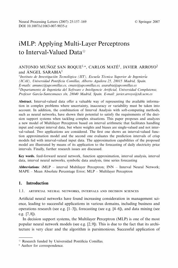
Table 1. Explanatory variables applied to the model.

Input Description

E(t) Total amount of traded energyN(t) Nuclear generationC(t) Coal generationF(t) Fuel generationG(t) Gas generationH(t) Hydro generationP(t −1) Electricity price for the previous dayP(t −7) Electricity price one week before

consumers and external agents perform electricity transactions. The main part ofthis energy is traded on the daily market. The purpose of the daily market, asan integral part of the electricity power production market, is to handle electric-ity transactions for the following day by the presentation of electricity sale andpurchase bids by market participants. The clearance of this market establishes anhourly clearing price which is paid to generators.

In this illustrative example, the daily electricity price interval is modelled asa function of the total amount of traded energy and the production coveredby different technologies: nuclear, coal, fuel, gas and hydro (see Table 1 for asummary of the variables considered). Regular and seasonal autoregressive com-ponents of the time series are modelled by including delayed electricity prices(orders 1 and 7) as input variables. All these inputs are also treated as dailyintervals.

An iMLP with 10 neurons in the hidden layer has been trained with 14 monthsof data as training set (Jul-1-2003 to Aug-31-2004) and validated with 3 months(Sep-1-2004 to Nov-30-2004). The same weight, β = 0.5, has been assigned inthe cost function to the prediction of centres and radii. Figure 2 shows the realand estimated prices for the training set, where a Mean Absolute PercentageError (MAPE) of 8.86% has been obtained for the center and 25.83% for itsradius.

In the case of the validation set (see Figure 3), the MAPE has reached a valueof 11.38% for the price centre and 24.54% for the radius. The similarity of thesemeasures with the above in the training set confirms the generalization capabilityof the proposed model.

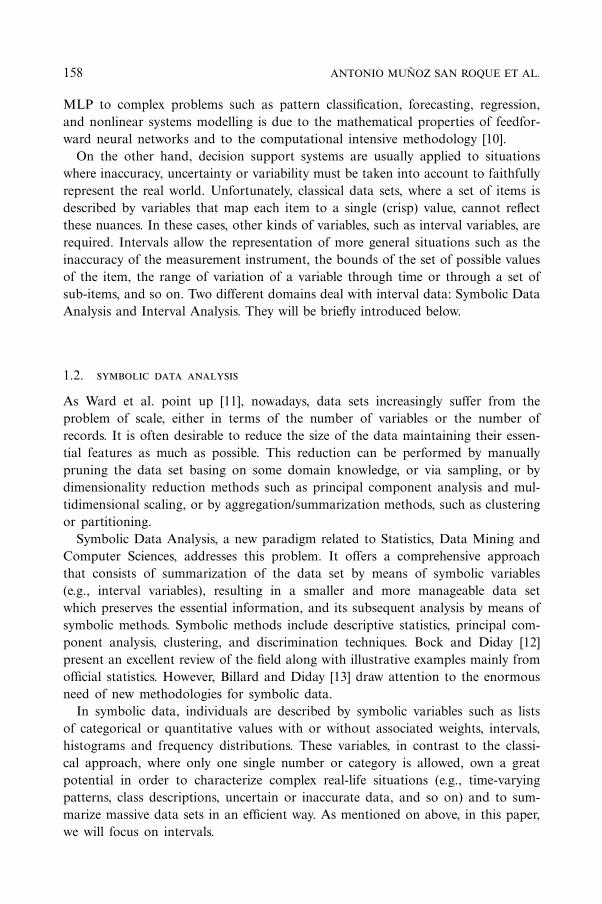
Table 2 compares the performance of the iMLP with a naıve reference modelthat proposes the observed price interval one week before as daily price intervalforecast.

These results confirm the predictability of the mean daily price as a function ofthe generation mix and its associated costs (similar error rates have been publishedin the literature: see [27] and [28] for more elaborate reference models), accompaniedby a high degree of random volatility affected by market participants’ strategies.


Figure 2. Training set estimation with iMLP(8,10,1).

Figure 3. Validation set estimation with iMLP(8,10,1).


Table 2. Comparison of the forecasting performance between theiMLP and the naive model with stationality.

Training set MAPE Validation set MAPE

Centre (%) Radius (%) Centre (%) Radius (%)

Naive model 15.85 33.82 17.86 33.44iMLP 8.86 25.83 11.38 24.54

5. Conclusions

In this paper, a new model of MLP is proposed in order to handle interval-valued data. The proposed model has the architecture of a standard MLP withsingle-valued weights and bias, but its transfer function has been modified in orderto operate with interval-valued inputs and outputs. The resulting model maps aninput vector of intervals to an interval output by means of interval arithmetic.

Two applications of the iMLP have been considered. First, as an interval-valuedfunction approximation model; and second, as a model that facilitates the evalua-tion of the prediction intervals of crisp MLP fed with interval-valued input data.

In the function approximation case, the parameters of the model are optimizedby minimizing a cost function defined in terms of discrepancies between estimatedand desired output intervals. The proposed cost function is a weighted sum of mid-points and radii squared estimation errors. The averaging weights in the error func-tion allow tuning the importance assigned to midpoints and to radii according toeach specific context. A backpropagation rule for the computation of the gradienthas also been derived. The computation of the prediction intervals of a crisp MLPsubject to input uncertainty is a straightforward result of the proposed architec-ture: once the crisp MLP has been trained with single-valued inputs and outputs,its response to interval inputs can be obtained directly by evaluating an iMLP withthe same weights.

The first application has been illustrated in this paper by applying the iMLP toforecast daily electricity prices intervals as a function of the generation mix. Thesecond one remains as ongoing work. Other extensions of the present work wouldinclude:

– The application of sensitivity analysis in order to quantify the effect of inputmidpoints and radii on the outputs of the iMLP.

– The application of iMLP to fuzzy regression analysis.– Proposing MLPs models based on the iMLP for other types of symbolic data

such as histograms, boxplots or distributions.

References

1. Smith, K. A.: Applications of neural networks. Comp. Oper. Res., 32(10) (2005),2495–2497


2. Smith, K. A. and Gupta J. N. D.: Neural networks in business: techniques and applica-tions for the operations researcher. Comp. Oper. Res., 27(11–12) (2000), 1023–1044.

3. Wong, B. K., Lai, V. S. and Lam, J.: A bibliography of neural networks business applica-tions research: 1994–1998. Comp. Oper. Res., 27(11–12) (2000), 1045–1076.

4. Perez, M.: Artificial neural networks and bankruptcy forecasting: A state of the art.Neural Comput. Appl., 15(2) (2006), 154–163.

5. Zhang, G., Patuwo, B. E. and Hu, M. Y.: Forecasting with artificial neural networks: Thestate of the art. Int. J. Forecast., 14(1) (1998), 35–62.

6. Zhang, G. P.: An investigation of neural networks for linear time-series forecasting.Computers and Operations Research, 28(12) (2001), 1183–1202.

7. Craven, M. W. and Shavlik, J. W.: Using neural networks for data mining. Future Gener.Comp. Syst., 13(2–3) (1997), 211–229.

8. Pal, S. K., Talwar, V. and Mitra, P.: Web mining in soft computing framework: relevance,state of the art and future directions. IEEE Trans. on Neural Networks 13(5) (2002),1163–1177.

9. Bishop, C. M.: Neural Networks for Pattern Recognition. Oxford University Press:Oxford, 1995.

10. Fine, T. L.: Feedforward Neural Network Methodology. Springer-Verlag: New York, 1999.11. Ward, M., Peng, W. and Wang, X.: Hierarchical visual data mining for large-scale data.

Computational Statistics, 19 (2004), 147–158.12. Bock, H. H. and Diday, E.(eds.): Analysis of Symbolic Data: Exploratory Methods for

Extracting Statistical Information from Complex Data. Springer-Verlag: Berlin, 2000.13. Billard, L. and Diday, E.: From the statistics of data to the statistics of knowledge:

symbolic data analysis. J. Am. Stat. Asso. 98(462) (2003), 470–487.14. Moore, R. E.: Interval Analysis. Prentice-Hall: Englewood Cliffs, NJ, 1966.15. Kearfott, B.: Interval computations: Introduction, uses, and resources. Euromath

Bull. 2(1) (1996), 95–112.16. Young, R. C.: The algebra of many-valued quantities. Mathematische Annalen, 104

(1931), 260–290.17. Beheshti, M., Berrached, R., de Korvin, A., Hu, C. and Sirisaengtaksin,O.: On inter-

val weighted three-layer neural networks. In: Proceedings of the 31st Annual SimulationSymposium, pp. 188–195, Boston, MA, USA, 1998.

18. Ishibuchi, H., Tanaka, H. and Okada, H.: An architecture of neural networks with inter-val weights and its application to fuzzy regression analysis. Fuzzy Sets Syst. 57 (1993),27–39.

19. Baker, M. R. and Patil, R.: Universal approximation theorem for interval neuralnetworks, Reliab. Comput. 4 (1998), 235–239.

20. Simoff, S. J.: Handling uncertainty in neural networks: An interval approach. In:Proceedings of IEEE International Conference on Neural Networks, pp. 606–610,Washington, DC, USA, 1996.

21. Drago, G. P. and Ridella, S.: Possibility and necessity pattern classification using aninterval arithmetic perceptron. Neural Comput. Appl., 8(1) (1999), 40–52.

22. Rossi, F. and Conan-Guez, B.: Multilayer perceptron on interval data. In: K. Jajuga,A. Sokolowski and H. H. Bock (eds.), Classification, Clustering, and Data Analysis(IFCS 2002), pp. 427–434, Cracow, Poland, 2002.

23. Patino-Escarcina, R., Callejas Bedregal, B. and Lyra, A.: Interval computing in neuralnetworks: One layer interval neural networks. In: G. Das and V. P. Gulati (eds.), Proceed-ings of the 7th International Conference on Information Technology, CIT 2004, pp. 68–75,Hyderabad, India, 2004.


24. Rumelhart, D. E., Hinton, G. E. and Williams, R. J.: Learning internal representa-tions by error propagation. In: D. E. Rumelhart and J. M. McClelland (eds.), Paralleldistributed processing: explorations in the microstructure of cognition, vol. 1: foundations,pp. 318–362, MIT Press: Cambridge, MA, USA, 1986.

25. Girosi, F., Jones, M. and Poggio, T.: Regularization theory and neural networks architec-tures. Neural Comput. 7(2) (1995), 219–269.

26. Luenberger, D. G.: Linear and Nonlinear Programming. Reading, MA: Addison-Wesley1984.

27. Bunn, D. W. (ed.): Modelling Prices in Competitive Electricity Markets. John Wiley &Sons: Chichester, UK, 2004.

28. Mateo Gonzalez, A., Munoz San Roque, A. and Garcıa Gonzalez, J.: Modeling andforecasting electricity prices with input/output hidden Markov models. IEEE Trans. onPower Syst. 20(1) (2005), 13–24.

iMLP: Applying Multi-Layer Perceptrons to Interval-Valued Data

Documents