Imaging rainfall drainage within the Miami oolitic limestone using high-resolution time-lapse ground-penetrating radar

Imaging rainfall drainage within the Miami oolitic limestone

using high-resolution time-lapse ground-penetrating radar

Steven Truss,1,2 Mark Grasmueck,1 Sandra Vega,1,3 and David A. Viggiano1

Received 1 July 2005; revised 19 August 2006; accepted 29 September 2006; published 6 March 2007.

[1] The vadose zone of the Miami limestone is capable of draining several centimeters ofrainfall within a fraction of an hour. Once the water enters the ground, little is knownabout the flow paths in the oolitic rock. A new rotary laser-positioned ground-penetratingradar (GPR) system enables centimeter-precise and rapid acquisition of time-lapse surveysin the field. Two-dimensional (2-D) GPR time-lapse surveying at a 3-min intervalbefore, during, and after rainfall shows how buried sand-filled dissolution sinks efficientlydrain the bulk of the rainwater. Hourly repeated 3-D imaging of a dissolution sink inresponse to surface infiltration shows how the wetting front propagates at a rate of0.6–1.2 m/h traversing the 5-m-thick vadose zone within hours. At the same time, some ofthe water migrates laterally into the host rock guided by stratigraphic unit boundaries.Average lateral propagation measured over a 28-hour period was of the order of 0.1 m/h.On a seasonal time frame, redistribution involves the entire rock volume. Comparing 3-Dsurveys acquired after wet summer and dry winter conditions shows good GPR eventcorrespondence, but also time shifts up to 20 ns caused by the change of overall watercontent within the vadose zone. High-precision time-lapse GPR imaging can therefore beused to noninvasively characterize natural drainage inside the vadose zone ranging fromtransient loading to seasonal variation.

Citation: Truss, S., M. Grasmueck, S. Vega, and D. A. Viggiano (2007), Imaging rainfall drainage within the Miami oolitic

limestone using high-resolution time-lapse ground-penetrating radar, Water Resour. Res., 43, W03405, doi:10.1029/2005WR004395.

1. Introduction

[2] Subsurface fluid flow in carbonates is often controlledby a highly heterogeneous hydraulic conductivity fieldresulting from the interplay of small-scale sedimentarystructure, diagenetic alteration, and fracturing [Duerrastand Siegesmund, 1999]. Rainfall/water table response times,well drawdown tests, slug tests, pump tests, and tracerexperiments exhibit surprisingly high hydraulic conductiv-ities, orders of magnitude higher than those derived frommeasurements on rock plugs taken from both outcrops andcores [Tidwell and Wilson, 1997]. Three-dimensional con-nectivity creates preferential flow paths allowing largevolumes of water, nutrients, and contaminants to rapidlybypass the less permeable bulk rock volume. For example,in large parts of urban Miami the vadose zone is charac-terized by oolitic carbonates, where laterally varying small-scale stratigraphy and crosscutting dissolution featurescontrol transport pathways [Cunningham, 2004]. Waterfrom heavy summer storms that ponds on the surface todepths of several centimeters disappears within a fraction ofan hour. Subsequent to the rapid infiltration, little is knownregarding the nature of water flow paths and rates in this

complex environment. It is essentially impossible to char-acterize drainage using standard hydrogeological methods.Traditional investigations rely on interpolation betweenpoint measurements (rock samples and borehole tests),and/or low resolution two-dimensional (2-D) geophysicalmethods (e.g., surface or borehole resistivity and electro-magnetic techniques). Even combined, these methods lackthe resolution to describe how or where the water is movingon the centimeter to meter scales.[3] This paper demonstrates how densely sampled and

precisely repeated ground-penetrating radar (GPR) surveyscan track fluid movement and characterize the subsurfaceflow regime at a field site in the Miami oolitic limestone.The objectives are twofold. The first is to test which of threeend-member conceptual models describing water flow (plugflow, lateral flow, bypass flow) within the Miami oolite areeffective in draining large amounts of rainwater into thesubsurface. As bypass flow emerges to be the dominantflow regime, the second objective is to image how waterenters the subsurface and spreads out in the limestone viainfilled dissolution holes. This case study shows field-scalechanges in densely sampled 2-D and 3-D GPR time-lapsedata in response to water infiltration at decimeter resolution,sourced from both rainfall and artificial injection within a5-m-thick natural vadose zone.

2. Time-Lapse GPR Method

2.1. Background

[4] Ground-penetrating radar (GPR) can noninvasivelydetect and image sedimentary structure to depths ranging

1Division of Marine Geology and Geophysics, Rosenstiel School ofMarine and Atmospheric Science, University of Miami, Miami, Florida,USA.

2Now at School of Earth and Environment, University of Leeds, Leeds,U.K.

3Now at the Petroleum Institute, Abu Dhabi, United Arab Emirates.

Copyright 2007 by the American Geophysical Union.0043-1397/07/2005WR004395

W03405

WATER RESOURCES RESEARCH, VOL. 43, W03405, doi:10.1029/2005WR004395, 2007

1 of 15

from 0 m to over 30 m [e.g., Smith and Jol, 1992; Aspironand Aigner, 1997, 1999; Beres et al., 1999; Corbeanu et al.,2001; Best et al., 2003; Grasmueck et al., 2004; Heinz andAigner, 2004; Neal, 2004]. Depth range depends on theelectrical conductivity of the subsurface material and GPRantenna frequency [Davis and Annan, 1989]. Clay-freematrix, air or fresh water in the pore space, and low signalfrequency offer the best conditions for deep GPR imaging.The main cause for GPR reflections are boundaries follow-ing changes in water content [Van Dam and Schlager,2000]. GPR has been successfully used to detect subsurfacemoisture [Greaves et al., 1996; Van Overmeeren et al.,1997; Gloaguen et al., 2001; Hubbard et al., 2002; Grote etal., 2003; Lambot et al., 2006]. With the sensitivity tochanges in water content, GPR has great potential tomonitor dynamic changes in the near surface. If a GPRsurvey is repeated with identical geometry, variationsbetween time series radar images must be due to watermovement as the internal geometry of the soil and rockvolume remains unchanged. Repeated GPR surveys havetracked fluid flow in laboratory tests and in the shallowsubsurface [Brewster and Annan, 1994; Birken andVersteeg, 2000; Endres et al., 2000; Trinks et al., 2001;Tsoflias et al., 2001; Binley et al., 2001, 2002; Versteeg,2002; Bevan et al., 2003]. These previous studies have thefollowing limitations in defining and characterizing prefer-ential flow in natural environments: (1) Coarse data acqui-sition: Wider than quarter wavelength profile spacingundersamples the electromagnetic wave field preventingthe use of 3-D migration processing to remove out-of-planereflections and focus diffractions [Grasmueck et al., 2005].(2) Lab experiments struggle to represent field conditions:Sand box experiments only image a small volume ofdisturbed soil with interfering GPR reflections from theenclosure walls. (3) Limited access by boreholes: Boreholetime-lapse GPR surveys image just the plane betweenboreholes, providing limited information on the 3-D natureof flow geometry. (4) Difficulty of repeating GPR surveysin the field: Surface time-lapse GPR surveys of field sitesare challenged with precise repeatability of the recordinglocations and data acquisition speed, reducing the ability todetect changes in the subsurface.[5] Changes in GPR signature due to water flow in the

subsurface are visible as amplitude changes and time shifts.Amplitude variations are due to changes in dielectriccontrast between layers which alter the reflection coeffi-cient. Within the unsaturated zone, a water content increaseoften enhances reflectivity contrasts and causes the GPRamplitudes to increase [Nobes et al., 2004]. Time shiftsoccur because increasing water content results in an increasein bulk dielectric constant which lowers the velocity andhence increases travel time, causing the reflection to appearat later recording times. Even in laboratory experiments[Trinks et al., 2001; Versteeg, 2002] with perfect repeatabil-ity and high data density, subtraction of repeated GPRsurveys produces strong, spurious amplitude differences inzones unaffected by fluid infiltration. The fluid anomaliescause cumulative time shifts in the data at later two-waytravel times, preventing cancellation of difference ampli-tudes in static zones after the electromagnetic wave haspassed a wetted zone. Such time shifts make differenceanalysis a highly unstable operation [Birken and Versteeg,

2000], requiring frequent survey repetition to minimize timeshifts between surveys.[6] Whereas time-lapse seismic monitoring of hydrocar-

bon production is becoming widespread and practical[Calvert, 2005], the potential of time-lapse GPR for near-surface applications has not yet been fully realized. Time-lapse GPR imaging of the vadose zone can be used tomonitor groundwater infiltration, contaminant migration,leaking pipes, irrigation efficiency, plant root water uptake,and fertilizer distribution. For time-lapse imaging at fieldsites to become effective, we have developed a new GPRdata acquisition system and field procedures addressing therequirements of rapid data collection and centimeter-preciseantenna positioning.

2.2. Time-Lapse GPR Data Acquisition at Field Sites

[7] Novel rotary laser positioning system (RLPS) tech-nology was integrated with GPR into a highly efficient andsimple to use 3-D imaging system [Grasmueck andViggiano, 2007]. The new system enables acquisition ofcentimeter-accurate x, y, and z coordinates from multiplesmall detectors attached to moving GPR antennae. Lasercoordinates streaming with 20 updates per second from eachdetector are fused in real time with the GPR data. For all thesurveys reported here we used a bistatic, shielded 250-MHzGPR antenna and the CU-II control unit (Mala Geosciences)modified for integration with the RLPS. Antenna offsetbetween transmitter and receiver was 0.36 m, and werecorded 602 samples per trace, eight stacks, and a samplinginterval of 0.325 ns resulting in a maximum two-way traveltime of 196 ns.[8] For imaging of changes in the near surface it is very

important that all repeated surveys are conducted withexactly the same survey geometry. Field tests with250-MHz GPR antennae by Grasmueck and Viggiano[2005] showed that reoccupation errors of survey positionsshould be in the range of 1–3 cm. With such precision,subtraction of two ‘‘identical’’ repeat 3-D GPR data setsacquired during static subsurface conditions yields a differ-ence volume with a root-mean-square (RMS) amplitudelevel 5–10 times lower than the RMS amplitude level inthe original surveys. This ensures low repeatability noiseand high sensitivity to changes in subsurface water content.For centimeter-precise reproduction of antenna positionsduring our field surveys we precisely followed a movablestring guideline tensioned between two parallel fiberglassmeasuring tapes anchored in the ground by plastic stakes.As it takes time to acquire each time-lapse data set, surveysize and repetition rate are closely linked. In order todetermine the GPR survey repetition rates and to obtain afirst assessment on where and how fast fluids are flowing,initial surveys consisting of repeated 2-D profiles wereconducted. The next stage of our survey strategy involvedacquisition of 3-D GPR surveys consisting of denselyspaced, parallel 2-D profiles in one direction over areas ofsuspected preferential flow paths. Full-resolution GPRimaging requires at least quarter wavelength grid spacingin all directions [Grasmueck et al., 2005]. For example, gridspacing for a spatially unaliased 250-MHz GPR survey hasto be 10 cm or less assuming 0.1 m/ns electromagnetic wavevelocity. By starting a new GPR survey at regular timeintervals, and acquiring each survey in the same profilesequence at an average antenna speed of 0.5 m/s, all

2 of 15

W03405 TRUSS ET AL.: IMAGING DRAINAGE USING TIME-LAPSE GPR W03405

subsurface points are imaged at constant time intervals.However, there is a time difference between recording thefirst and the last trace of each GPR survey. As the water iscontinuously migrating through the subsurface, the wettingfronts imaged in the GPR are not instant snapshots, but areslightly skewed with a linear acquisition time delay.

2.3. Data Processing

[9] All GPR data acquired during a time-lapse survey areprocessed in exactly the same way. We use a combination ofprocessing modules we developed in LabView (NationalInstruments) and, where mentinoned, commercially avail-able seismic processing software. The seismic industrystandard (SEGY) data format facilitates data transferbetween different software applications. The processingsteps are as follows: (1) ‘‘Data fusion’’ assigns laser-derivedx, y, and z coordinates to each radar trace acquired. As aresult, the GPR tracklines can be plotted on a map.(2) ‘‘Detrending’’ compensates for zero time drift due totemperature changes affecting the GPR electronics byautomatic picking of first breaks. The spatially smootheddifferences between the first break picks and a referencefirst break time are applied as vertical time shifts to traces.The smothing is applied to reduce the effect of random firstbreak jitter. This step also removes zero time shifts betweenindividually recorded data sets aligning all first breaks toone comon level throughout a survey and also betweenrepeat surveys. (3) The zero time is adjusted by delaying thefirst break by the time it takes the direct airwave to travelfrom transmitter to receiver. (4) The ‘‘dewow’’ [Annan,2003] step removes very low frequency components of thedata associated with either inductive phenomena or analog/digital conversion. (5) The same gain curve is applied to alldata aquired within a time-lapse series. The gain curve isbased on a smoothed Hilbert transform of a representativedata volume. (6) Regularization populates an identical bingrid for all surveys with the nearest available trace. For 2-Dtime-lapse surveys the regularization creates a pseudo 3-Ddata volume, with one of the horizontal axes displaying theacquisition time of the first trace recorded for each 2-D line.For the 3-D time-lapse surveys a new 3-D GPR data volumeis generated for each repeat. (7) Velocity estimates are basedon diffraction hyperbola analysis with ReflexW (SandmeierScientific Software). For the experiments reported inthis paper we analyzed diffractions in the ‘‘dry’’ surveysacquired before rain or infiltration. (8) Normal-moveout(NMO) stretching [Yilmaz, 2000] of the GPR signal tracescompensates for the transmitter-receiver offset of 0.36 m.This and the following migration step both use the sameconstant velocity model. (9) Migration processing is appliedto increase the resolution of 3-D GPR data. GPR antennaehave a wide-open antenna radiation cone (as much as 60�radiation angle measured from the vertical) which simulta-noeusly receives both vertical and side reflections. Migra-tion focuses diffractions and repositions dipping reflections.We did not apply migration processing to 2-D GPR data fortwo reasons: to clearly show the presence of diffractionhyperbolae indicative of local heterogeneities, e.g., causedby finger flow, and because migration processing requireshigh-density 3-D GPR data acquired with at least a quarter-wavelength grid spacing in all directions [Grasmueck et al.,2005]. Applying migration to 2-D data produces spuriousresults. For the 3-D time-lapse data we used the Promax

(Landmark Graphics Corporation) 3-D phase-shift migra-tion with a constant velocity model. (10) For analysis of thechanges between repeat surveys, corresponding data areeither visually compared or subtracted to highlight thedifferences.

3. Miami Oolitic Limestone Vadose Zone CaseStudy

3.1. Geological Setting

[10] The oolitic facies of the Miami limestone (MiamiOolite) was deposited as a network of Pleistocene (125 ka)ooid shoals, tidal channels, and seaward barrier bars duringan interglacial sea level high-stand, where sea levels wereapproximately 6–7 m higher than today [Halley et al.,1977; Halley and Evans, 1983]. Modern topography stilloutlines the paleogeography (Figures 1a and 1b) and con-sists of a 50-km-long and 10-km-wide elevated coastal ridgeextending along Florida’s east coast [Hoffmeister et al.,1967]. Our field sites are located along this ridge, in theCoral Gables and Coconut Grove area of Miami, where thetopography is highest and therefore the vadose zone isthickest (4–7 m). The Ingraham Public Park offers a 5-m-high vertical outcrop (Figure 2) close to the location ofall GPR surveys reported here. The waterway next tothe site causes a brackish water table at 5-m depth, limitingGPR imaging to the vadose zone above. Because largeexcavations were not permitted in the public park, we inves-tigated two ongoing excavations at nearby active constructionsites on Galiano Street and Franklin Avenue for fresh expo-sures of the Miami Oolite and its related dissolution features.[11] Halley and Evans [1983] described three distinct

facies in the Miami limestone: (1) the bedded (cross-beddedoolite), (2) mottled (heavily bioturbated), and (3) Bryozoanfacies. Lateral variations within the facies typically occur at ascale of 10 m, and facies of type 1 and 2 are exposed in theoutcrop at the southern end of the Ingraham test site(Figure 2). High-energy, prograding ooid shoals with a highlyvariable internal structure and varying degrees of cementationlie directly upon low-energy, bioturbated, mottled limestone.The ooid shoal deposits display abundant large-scale (up to1 m between erosive surfaces) cross bedding, often gradingdown into ripple bedding (1–2 cm foresets in 5–20 cmpackets). This highly variable rock structure results in a widevariety of pore sizes ranging from open, centimeter-sizedburrows to rocks with no visible porosity when viewed usinga hand lens. Rock plugs have shown porosities larger than40% and an average hydraulic conductivity of 10 mm/s.[12] Diagenetic processes have increased the degree of

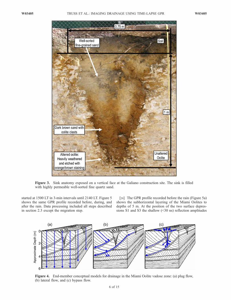
heterogeneity. Selective cementation, which often preservesand enhances small-scale sedimentary features, is common[Halley and Evans, 1983]. Large-scale karstic dissolutionholes tens of meters across are relatively uncommon, butsmaller-scale infilled dissolution holes 1–4 m in diameterand 1–4 m deep are abundant. Several holes that intersectthe water table have been observed both at the Franklin andthe Galiano construction sites, leading to the concept of‘‘sinks,’’ which are preferential pathways with the potentialto transfer fluids rapidly through the rock mass (Figure 3).Typically the sinks are infilled with a thin layer of darksandy top soil, with light brown fine quartz sand probablyof aeolian origin forming the core. The transition from light

W03405 TRUSS ET AL.: IMAGING DRAINAGE USING TIME-LAPSE GPR

3 of 15

W03405

brown sand fill into white oolite host rock is via dark brownsand with oolite clasts and a 10–50 cm thick layer oforange/brown-stained altered oolite. The dissolution processgenerally leaves a large, irregularly shaped contact surfacebetween the sink fill and the surrounding rock, assistingfluid transfer across the interface.

3.2. Conceptual Models for Rainfall Drainage

[13] The degree of rock heterogeneity strongly influencesthe nature of rainwater infiltration, affecting poststorm

drainage, groundwater recharge, and pollutant transport ina subtropical climate characterized by short-duration high-intensity rainfalls. Following heavy rainfall, several centi-meters of standing water drain completely into the rockmass within 15–30 min at the undisturbed Ingraham site,whereas some newly excavated rock surfaces at the nearbyFranklin Avenue construction site retain standing water forseveral days. Hence the undisturbed Miami oolitic lime-stone appears to be efficient at draining water from the

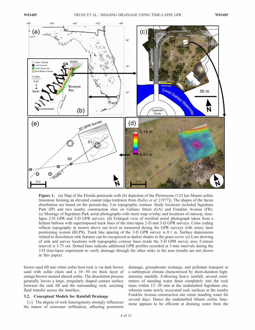
Figure 1. (a) Map of the Florida peninsula with (b) depiction of the Pleistocene (125 ka) Miami ooliticlimestone forming an elevated coastal ridge (redrawn from Halley et al. [1977]). The shapes of the faciesdistribution are based on the present-day 3-m topographic contour. Study locations included IngrahamPark (IP) and two nearby construction sites on Galiano Street (GA) and Franklin Avenue (FR).(c) Montage of Ingraham Park aerial photographs with street map overlay and locations of outcrop, time-lapse 2-D GPR and 3-D GPR surveys. (d) Enlarged view of rectified aerial photograph taken from ahelium balloon with superimposed track lines of the time-lapse 2-D and 3-D GPR surveys. Color codingreflects topography in meters above sea level as measured during the GPR surveys with rotary laserpositioning system (RLPS). Track line spacing of the 3-D GPR survey is 0.1 m. Surface depressionsrelated to dissolution sink features can be recognized as darker shades in the grass cover. (e) Line drawingof sink and survey locations with topographic contour lines inside the 3-D GPR survey area. Contourinterval is 3.75 cm. Dotted lines indicate additional GPR profiles recorded at 3-min intervals during the2-D time-lapse experiment to verify drainage through the other sinks in the area (results are not shownin this paper).

4 of 15

W03405 TRUSS ET AL.: IMAGING DRAINAGE USING TIME-LAPSE GPR W03405

frequent tropical summer storms, even if some of the indi-vidual rock layers are resistant to vertical water movement.[14] To help explain this dichotomy, three end-member

conceptual models describing water flow within the MiamiOolite are illustrated in Figure 4. The three models are(1) plug flow, (2) lateral flow, and (3) bypass flow.[15] 1. In the plug flow model the rainfall enters the

ground and travels vertically toward the water table, in amanner independent of stratigraphy. This model assumesthat the lateral hydraulic gradient is always small comparedwith the vertical hydraulic gradient, so that all flow isdirectly downward. Hence the flow rate within the rockmatrix will be a function of the pore size distribution and thehydraulic gradient. This is the model most used in flowsimulations, and while it normally suffices on a whole-aquifer scale, it has limitations when applied at field-sitescale by not accounting for geological heterogeneity.[16] 2. In the lateral flow model the rainfall travels along

stratigraphic pathways that follow sedimentary structure.This model is dependent on hydraulic conductivity varia-tions, which are controlled by lithology, biological action,and diagenesis. In this case, relatively impermeable zonesretard water movement, causing localized pressure headconditions. These provide a hydraulic force which can besufficient to drive the water in a nonvertical manner,following more permeable horizons situated directly aboveless permeable ones [Truss, 2004]. Under normal rainfallconditions the water flow obeys Darcy’s law, but it ispossible that at extremely high loadings sufficient hydro-static pressure may be available to force water out of therock matrix and into the centimeter-sized karstic macro-pores and allow free draining to occur.[17] 3. In the bypass flow model, storm rainfall flows

laterally along the ground surface and fills slight surfacedepressions above sand-filled dissolution sinks (Figure 3)which provide a rapid pathway to the deeper subsurface.‘‘Flooding’’ of the sink allows the initiation of largepressure heads which are able to overcome matric pressureand ‘‘force’’ fluids into the surrounding rock. Under theseconditions fluids flow at a much greater rate than in thecases of plug flow or lateral flow, possibly initiating non-Darcyan flow under significantly lower rainfall loadings.Once expelled from the sink and into the rock mass, thewater flows as per plug or lateral flow.

[18] The true nature of water infiltration is likely to be acontinuum between these three end- members, which mayvary as rainfall loading and initial saturation values changeseasonally. Using repeated 2-D and 3-D GPR surveys wetested the validity of these three models for rainfall andartificial infiltration.

3.3. Rapid 2-D Time-Lapse GPR Monitoring ofRainfall Infiltration

[19] The purpose of this time-lapse 2-D GPR surveyingbefore, during, and after rainfall was to determine which ofthe three conceptual flow models was the prevalent drainingmechanism: whether the water was evenly soaking into theground, moving along permeable stratigraphic layers, orpassing through infilled vertical sinks. In order to capturerapid drainage patterns we acquired a series of repeat radarprofiles at 3-min intervals. Initial tests using an odometerwheel to position the GPR measurements along a fixedprofile proved to be too inaccurate for data differencing tohighlight the changes caused by water infiltration. Repeat-ability noise due to positioning errors was prevalent. In asecond series of experiments we used the new laser-positioned GPR system [Grasmueck and Viggiano, 2007].For the best repeatability of the GPR profiles we chosestraight lines (instead of a curved path) directly crossingover surface depressions to determine if they were activesinks. From the air (Figures 1d and 1e) such depressions canbe recognized by their darker shade of green when com-pared with the surrounding grass. During rainfall, thedepressions develop into shallow puddles. We continuouslyrecorded a loop of three profiles, starting a new loop every3 min, as it took 1 min to record each profile. Results from allthree profiles were similar so we selected only the 24-m-longprofile 1 crossing depressions S1 and S3 for display inFigures 5, 6, and 7. The first set of repeat GPR lines wasrecorded on 10 March 2006 in dry conditions, 14 days afterthe last 37 mm of rain and a total of 117 mm of rain over thelast 3 months. The start and end points were permanentlymarked with survey nails for precise relocation during latersurveys. We waited for the first rainfall, which occurred on23 March 2006 in two showers. The first shower started at1420 LT, yielding 22.5 mm of rain in 50 min. Another12 mm of rain followed in a second shower between 1650and 1710 LT. The continuous recording of GPR profiles

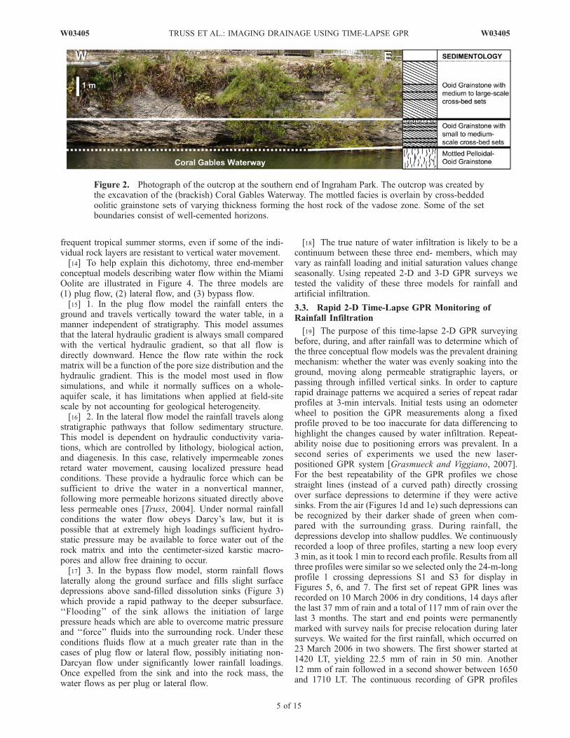
Figure 2. Photograph of the outcrop at the southern end of Ingraham Park. The outcrop was created bythe excavation of the (brackish) Coral Gables Waterway. The mottled facies is overlain by cross-beddedoolitic grainstone sets of varying thickness forming the host rock of the vadose zone. Some of the setboundaries consist of well-cemented horizons.

W03405 TRUSS ET AL.: IMAGING DRAINAGE USING TIME-LAPSE GPR

5 of 15

W03405

started at 1500 LT in 3-min intervals until 2140 LT. Figure 5shows the same GPR profile recorded before, during, andafter the rain. Data processing included all steps describedin section 2.3 except the migration step.

[20] The GPR profile recorded before the rain (Figure 5a)shows the subhorizontal layering of the Miami Oolites todepths of 5 m. At the position of the two surface depres-sions S1 and S3 the shallow (<30 ns) reflection amplitudes

Figure 3. Sink anatomy exposed on a vertical face at the Galiano construction site. The sink is filledwith highly permeable well-sorted fine quartz sand.

Figure 4. End-member conceptual models for drainage in the Miami Oolite vadose zone: (a) plug flow,(b) lateral flow, and (c) bypass flow.

6 of 15

W03405 TRUSS ET AL.: IMAGING DRAINAGE USING TIME-LAPSE GPR W03405

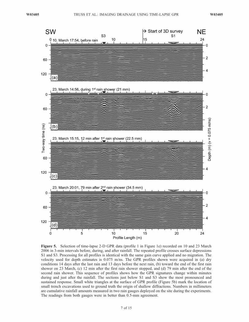
Figure 5. Selection of time-lapse 2-D GPR data (profile 1 in Figure 1e) recorded on 10 and 23 March2006 in 3-min intervals before, during, and after rainfall. The repeated profile crosses surface depressionsS1 and S3. Processing for all profiles is identical with the same gain curve applied and no migration. Thevelocity used for depth estimates is 0.075 m/ns. The GPR profiles shown were acquired in (a) dryconditions 14 days after the last rain and 13 days before the next rain, (b) toward the end of the first rainshower on 23 March, (c) 12 min after the first rain shower stopped, and (d) 79 min after the end of thesecond rain shower. This sequence of profiles shows how the GPR signatures change within minutesduring and just after the rainfall. The sections just below S1 and S3 show the most pronounced andsustained response. Small white triangles at the surface of GPR profile (Figure 5b) mark the location ofsmall trench excavations used to ground truth the origin of shallow diffractions. Numbers in millimetersare cumulative rainfall amounts measured in two rain gauges deployed on the site during the experiments.The readings from both gauges were in better than 0.5-mm agreement.

W03405 TRUSS ET AL.: IMAGING DRAINAGE USING TIME-LAPSE GPR

7 of 15

W03405

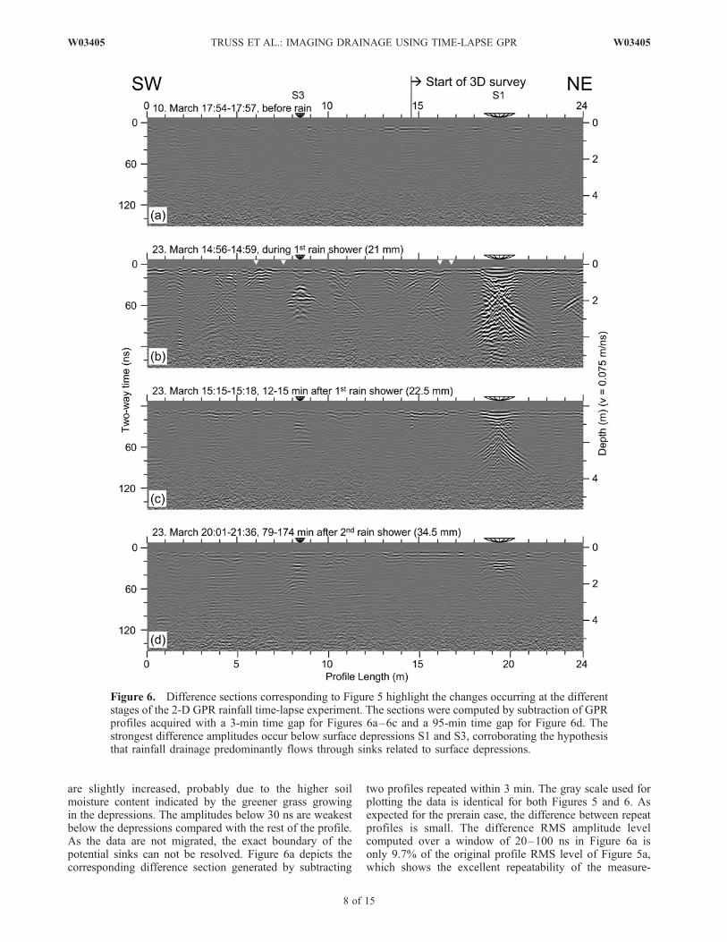
are slightly increased, probably due to the higher soilmoisture content indicated by the greener grass growingin the depressions. The amplitudes below 30 ns are weakestbelow the depressions compared with the rest of the profile.As the data are not migrated, the exact boundary of thepotential sinks can not be resolved. Figure 6a depicts thecorresponding difference section generated by subtracting

two profiles repeated within 3 min. The gray scale used forplotting the data is identical for both Figures 5 and 6. Asexpected for the prerain case, the difference between repeatprofiles is small. The difference RMS amplitude levelcomputed over a window of 20–100 ns in Figure 6a isonly 9.7% of the original profile RMS level of Figure 5a,which shows the excellent repeatability of the measure-

Figure 6. Difference sections corresponding to Figure 5 highlight the changes occurring at the differentstages of the 2-D GPR rainfall time-lapse experiment. The sections were computed by subtraction of GPRprofiles acquired with a 3-min time gap for Figures 6a–6c and a 95-min time gap for Figure 6d. Thestrongest difference amplitudes occur below surface depressions S1 and S3, corroborating the hypothesisthat rainfall drainage predominantly flows through sinks related to surface depressions.

8 of 15

W03405 TRUSS ET AL.: IMAGING DRAINAGE USING TIME-LAPSE GPR W03405

ments. The weak horizontal bands at the top of the profileare due to clipping of the first arrival amplitudes. As therepeat profiles were recorded in dry conditions, there shouldtheoretically be no change in the GPR signals of geologicalorigin. Therefore the faint difference amplitude patterns ofFigure 6a which are related to geological reflectors providea useful visual measure to help distinguish changes causedby water flow from GPR survey repeatability noise inFigures 6b–6d.[21] The GPR profile collected in pouring rain (Figure 5b)

shows enhanced amplitudes throughout. A similar effect hasbeen observed by Nobes et al. [2004]. The thin superficialfully saturated layer increases antenna coupling. The sinksdisplay the most amplitude enhancement. At the same time,numerous crisscross patterns caused by diffractions develop.The apices of the diffractions are either near the surface orinside the sinks. The cause of these diffractions is likely tobe the wetting front with a strong reflection coefficient atthe transition from wet to dry material. The diffractionsindicate the wetting front to have subwavelength-scaleirregularities such as finger flow causing the numerouspoint scatterers. To determine the cause of the diffractionsoriginating near the surface, we excavated four smalltrenches (30 cm � 30 cm) through the soil layer untilreaching the oolite rock surface. The two trenches at profilepositions 7.55 m and 16.75 m with no diffraction patternsrevealed a flat, contiguous rock surface with 19–24 cm ofsandy soil cover. The other two trenches at profile positions6.00 and 16.10 m featured 26–33 cm of sandy soil, ooliterubble, tree roots, and an irregular rock surface with finger-

sized sand-filled dissolution features. The diffractionsinvisible in dry conditions and appearing during rainfallare therefore an indication of small-scale preferential flowpaths besides the larger-scale sinks. The difference sectioncomputed between two profiles repeated within 3 minduring rain (Figure 6b) further highlights the diffractionpatterns and shows strong amplitudes everywhere caused byomnipresent time shifts. The superficial drenching withwater also causes time shifts on deeper geological reflec-tions unaffected by any water flow.[22] Only 12 min after the first rain shower stopped and

most of the superficial water had run off, Figures 5c and 6cshow more stable conditions with a decrease in amplitudesand diffraction patterns. The 3-min difference amplitudes ofthe surface reflections above sink S3 are back near therepeatability noise amplitude gray level of Figure 5a. Fieldlogs indicate the standing water at the surface of this sinkhad completely drained by the time this line was recorded.The difference amplitudes suggest drainage processes insink S3 were now active below 20 ns or about 0.75 m depth.In contrast, sink S1 was still flooded. Increased surfaceamplitude difference zones at profile locations 1.8–5.1 m,5.8–7.3 m, and 13.7–16.4 m indicate the zones identifiedby shallow diffractions had not completely drained yet.[23] The profile of Figure 5d acquired 79 min after the

second rain shower shows a further decrease in amplitudesand diffractions. Compared with Figure 5a the most signif-icant changes are associated with the sinks. Below sink S3,amplitudes have increased over the entire depth range, whilein sink S1 amplitude changes are confined to the top 100 ns.

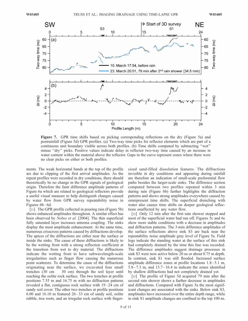
Figure 7. GPR time shifts based on picking corresponding reflections on the dry (Figure 5a) andpostrainfall (Figure 5d) GPR profiles. (a) Two-way time picks for reflector elements which are part of acontinuous unit boundary visible across both profiles. (b) Time shifts computed by subtracting ‘‘wet’’minus ‘‘dry’’ picks. Positive values indicate delay in reflector two-way time caused by an increase inwater content within the material above the reflector. Gaps in the curve represent zones where there wereno clear picks on either or both profiles.

W03405 TRUSS ET AL.: IMAGING DRAINAGE USING TIME-LAPSE GPR

9 of 15

W03405

It appears that sink S3 with a smaller diameter had beenflooded to the groundwater level at 5 m depth, bypassingthe entire vadose zone. For sink S1, water-related changesstop above the groundwater level. Difference plots over3-min intervals do not show any significant changes at thisstage of infiltration, clear evidence for a slowdown of theoperative flow processes. Increasing the time intervalbetween the subtracted profiles to 95 min (Figure 6d) showsthe strongest difference amplitudes below the surfacedepressions.[24] Similar GPR responses during and after rain confirm

all surface depressions shown in Figure 1e as active sinks.Interestingly, the spacing of sink depressions appears to berelated to the size of surface depression and underlying sink.Assuming the midpoints between sinks are watershedboundaries, circular watershed area estimates range from6 to 64 m2. As shown in the controlled infiltration exper-iment described in the next section, sink S1 is capable ofdraining 1100 L/h. On the basis of a 64-m2 watershed thissink could accommodate 17 mm/h rainfall as pure overlandflow. As the sink depressions fill with 5–10 cm of standingwater within minutes during rain showers, overland flowmust be very efficient in delivering large volumes of waterto the sinks.[25] GPR time shift analysis further elucidates the relative

importance of sink drainage versus drainage through thesurrounding soil and rock volume. In Figure 7 correspondingreflections of the same event were picked on the dry(Figure 5a) and well-drained (Figure 5d) GPR profiles. Bythe time this last profile was recorded, the grass andsuperficial soil had dried off, providing similar surfaceantenna coupling conditions to the dry case, thus allowingaccurate time comparisons of the deeper GPR events. Thesinks display pronounced time shifts up to +5 ns due towetting, while outside the sinks the time shifts range from�1 to +1.5 ns. For comparison, the 34.5 mm of rain evenlysoaking into the ground would only create a +2 ns shift atthe same depth according to the Topp equation for mineralsoils [Topp et al., 1980; Huisman et al., 2003]. Therefore the+5 ns shift within the sinks is clear evidence for rainwaterpreferentially draining through the sinks. If 100% of the34.5 mm of rain falling in the estimated 64-m2 watershedof sink S1 would be present in a vertical cylinder with across section of 6 m2 the time shift would be +24 ns.Several factors may explain the reduction to the observed+5 ns: (1) The dry GPR profile was recorded 12 days priorto the rain. The ground dried out during this time asevidenced by the �1 ns shift observed outside the sinks.(2) Some water is retained in the soil, especially in the zoneswith increased soil thickness and disturbed rock surfacecharacterized by the shallow diffractions during the rain.These are the zones in Figure 7 with up to +1.5 ns timeshifts outside the sinks. (3) The 34.5 mm of rain fell in twoshowers separated by 100 min. Some of the water from thefirst 22.5 mm rain shower probably already had flowed todeeper levels below the picked event at 65 ns. (4) The twoGPR profiles only give a bulk estimate of changes in watercontent. A 3-D time-lapse survey would better resolve thelocation of the flow and related changes.[26] In summary, the precisely positioned 2-D time-lapse

experiment recorded with a 3-min repeat rate established theimportance of sink drainage during and after rainfall.

Overland flow fills the surface depressions with water andthe sinks rapidly drain the water. An augering test revealedwell-sorted fine-grained sand as fill material very similar tothe fill material excavated from the sink in Figure 3. TheGPR data show the superficial saturation and infiltration tohappen within minutes during and shortly after the rainfall.Once the water enters the sinks, GPR survey repetition ratesof over 1 hour appear to be sufficient to capture the changestaking place in the subsurface. This opens the opportunity toacquire full-resolution 3-D surveys and apply 3-D migrationprocessing to better image the sinks and associated flowprocesses.

3.4. Full-Resolution 3-D Time-Lapse GPR Imagingof Flow Through a Dissolution Sink

[27] We selected sink S1 from the previous experiment asan example to image geometry and wetting front migration.For this experiment, the open end of a water hose wasattached to the ground with plastic pegs at the center of thesurface depression shown in Figure 1d. The sink was notaugered in order not to disturb the natural flow paths. Thewater was freely flowing out of the hose at a rate ofapproximately 1100 L/h over 4 hours. The total volume of4400 L is at least double the water infiltrated during therainfall experiment discussed in the previous section.Assuming 100% overland flow and no soil retention,34.5 mm of rain falling in a watershed of 64 m2 wouldyield only 2208 L.[28] Hourly repeated 3-D GPR surveys, covering an area

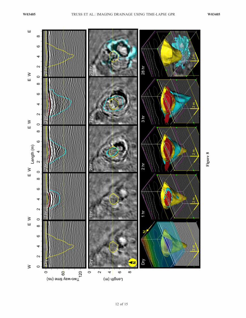
of 10 m � 10 m with parallel E-W oriented profiles spacedby 0.1 m (the track lines are visible in Figure 1d) werecollected with RLPS and a 250-MHz antenna. At an antennaspeed of 0.5 m/s, a GPR trace was acquired approximatelyevery 0.025 m for assignment into a 0.05 m � 0.10 mregularized data grid. It took 50 min to record each 3-Dsurvey. Each survey started in the SW corner of the surveyarea. Immediately before turning on the water, one ‘‘dry’’3-D data set was acquired. Three GPR surveys wereacquired while the water was running. The fifth data setwas acquired 28 hours after the infiltration had started(24 hours after the water shutoff) to see how the infiltratedwater would drain and redistribute over a longer time frame.The data recorded during the infiltration with standing wateron the surface were dominated by diffraction patternssimilar to those in Figure 5b. All data sets were processedin exactly the same way, including a Promax 3-D phase-shiftmigration utilizing a constant velocity of 0.075 m/ns. Thisvelocity was determined by analysis of diffraction hyperbolaein the dry 3-D survey acquired before infiltration. Themigration focused the diffractions and improved imagingof the sink and wetting fronts. The satisfactory focusing alsoat the later stages of the infiltration experiment indicatesthe 3-D migration to be relatively robust against thelocalized velocity changes caused by the infiltration ofwater. Because of time shifts caused by the increase inwater content, depth conversion becomes less accurate.Topographic corrections based on the z coordinates acquiredtogether with the GPR data were applied as time shifts to themigrated data volumes assuming a velocity of 0.075 m/ns.[29] Figure 8 shows different views of the migrated data

at five consecutive time instances of the infiltration exper-iment. The top row displays a vertical cross section takenfrom the center of the sink. The middle row consists of a

10 of 15

W03405 TRUSS ET AL.: IMAGING DRAINAGE USING TIME-LAPSE GPR W03405

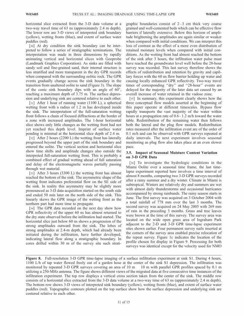
horizontal slice extracted from the 3-D data volume at atwo-way travel time of 63 ns (approximately 2.4 m depth).The lower row are 3-D views of interpreted sink boundary(yellow), wetting fronts (blue), and extent of surface waterpuddles (red).[30] At dry condition the sink boundary can be inter-

preted to follow a series of stratigraphic terminations. Theinterpretation was made in three dimensions by rapidlyanimating vertical and horizontal slices with Geoprobe(Landmark Graphics Corporation). As sinks are filled withsandy soil and fine-grained sand, their internal structure isless stratified and more transparent in the dry GPR recordswhen compared with the surrounding oolitic rock. The GPRevents gradually change across the sink boundary in thetransition from unaltered oolite to sand (Figure 3). The slopeof the conic sink boundary dips with an angle of 60�,reaching a maximum depth of 3.75 m. The surface depres-sion and underlying sink are centered relative to each other.[31] After 1 hour of running water (1100 L), a spherical

wetting front with a radius of 1.2 m has developed insidethe sink. The interpretation of the full-saturation wettingfront follows a chain of focused diffractions at the border ofa zone with increased amplitudes. The 1-hour horizontalslice shows only little changes as the wetting front had notyet reached this depth level. Imprint of surface waterponding is minimal at the horizontal slice depth of 2.4 m.[32] After 2 hours (2200 L) the wetting front has laterally

progressed beyond the upper part of the sink boundary andentered the oolite. The vertical section and horizontal sliceshow time shifts and amplitude changes also outside theinterpreted full-saturation wetting front. This is probably acombined effect of gradual wetting ahead of full saturationand delay of the electromagnetic waves partially passingthrough wet material.[33] After 3 hours (3300 L) the wetting front has almost

reached the bottom of the sink. The asymmetric shape of thewetting front indicates preferential flow on the SE side ofthe sink. In reality this asymmetry may be slightly morepronounced as 3-D data acquisition started on the south sideand ended 50 min later on the north side of the sink. Thislinearly skews the GPR image of the wetting front as thenorthern part had more time to propagate.[34] The GPR data recorded on the next day show how

GPR reflectivity of the upper 60 ns has almost returned tothe dry state observed before the infiltration had started. Thehorizontal slice just below 60 ns shows a progression of thestrong amplitudes outward from the sink. The lobes ofstrong amplitudes at 2.4-m depth, which had already beeninitiated during the infiltration, have further developed,indicating lateral flow along a stratigraphic boundary. Incores drilled within 30 m of the survey site such strati-

graphic boundaries consist of 2–3 cm thick very coarsegrained and well-cemented beds which can be effective flowbarriers if laterally extensive. Below this horizon of ampli-tude brightening the amplitudes are again similar or weakerwhen compared with initial conditions. We can interpret thisloss of contrast as the effect of a more even distribution ofretained moisture levels when compared with initial con-ditions. As the wetting front had almost reached the bottomof the sink after 3 hours, the infiltration water pulse musthave reached the groundwater level well before the 28-hoursurvey was recorded. This last survey therefore shows theeffects of redistribution and retention by gravity and capil-lary forces with the 60 ns flow barrier holding up water andcausing locally enhanced GPR reflectivity. Two-way traveltimes of corresponding ‘‘dry’’ and ‘‘28-hour’’ events aredelayed for the majority of the later data set caused by anoverall increase of water retained in the vadose zone.[35] In summary, this experiment clearly shows how the

three conceptual flow models asserted at the beginning ofthis paper operate at different timescales. Bypass flowrapidly transports the vast majority of the water withinhours at a propagation rate of 0.6–1.2 m/h toward the watertable. Redistribution of the remaining water then followsboth the lateral and the plug flow models. Redistributionrates measured after the infiltration event are of the order of0.1 m/h and can be observed with GPR surveys repeated atdaily intervals. The next experiment involves seasonalmonitoring as plug flow also takes place at an even slowerpace.

3.5. Impact of Seasonal Moisture Content Variationon 3-D GPR Data

[36] To investigate the hydrologic conditions in theMiami Oolite over a seasonal time frame, the last time-lapse experiment reported here involves a time interval ofalmost 8 months, comparing two 3-D GPR surveys recordedafter a rainy summer and a dry winter. Climate in Miami issubtropical. Winters are relatively dry and summers are wetwith almost daily thunderstorms and occasional hurricanesaccompanied by strong rainbands. The rainy season starts inJune. The first survey was acquired on 3 October 2004 witha total rainfall of 778 mm over the last 3 months. Thesecond survey was acquired on 24 May 2005 with 269 mmof rain in the preceding 3 months. Grass and tree leaveswere brown at the time of this survey. The survey area waslocated on the wide open grass area of Ingraham Parkadjacent to the 2-D and 3-D GPR time-lapse experimentsites shown earlier. Four permanent survey nails inserted atthe corners of the survey area enabled precise relocation ofthe repeat survey. Figure 1c indicates the location of theprofile chosen for display in Figure 9. Processing for bothsurveys was identical except for the velocity used for NMO

Figure 8. Full-resolution 3-D GPR time-lapse imaging of a surface infiltration experiment at sink S1. During 4 hours,1100 L/h of tap water flowed freely out of a garden hose at the center of the sink S1 depression. The infiltration wasmonitored by repeated 3-D GPR surveys covering an area of 10 m � 10 m with parallel GPR profiles spaced by 0.1 mutilizing a 250-MHz antenna. The figure shows different views of the migrated data at five consecutive time instances of theinfiltration experiment. The top row displays a vertical cross section taken from the center of the sink. The middle rowconsists of a horizontal slice extracted from the 3-D data volume at a two-way time of 63 ns (approximately 2.4 m depth).The bottom row shows 3-D views of interpreted sink boundary (yellow), wetting fronts (blue), and extent of surface waterpuddles (red). Topographic contours plotted on the top surface show how the surface depression and underlying sink arecentered relative to each other.

W03405 TRUSS ET AL.: IMAGING DRAINAGE USING TIME-LAPSE GPR

11 of 15

W03405

Figure

8

12 of 15

W03405 TRUSS ET AL.: IMAGING DRAINAGE USING TIME-LAPSE GPR W03405

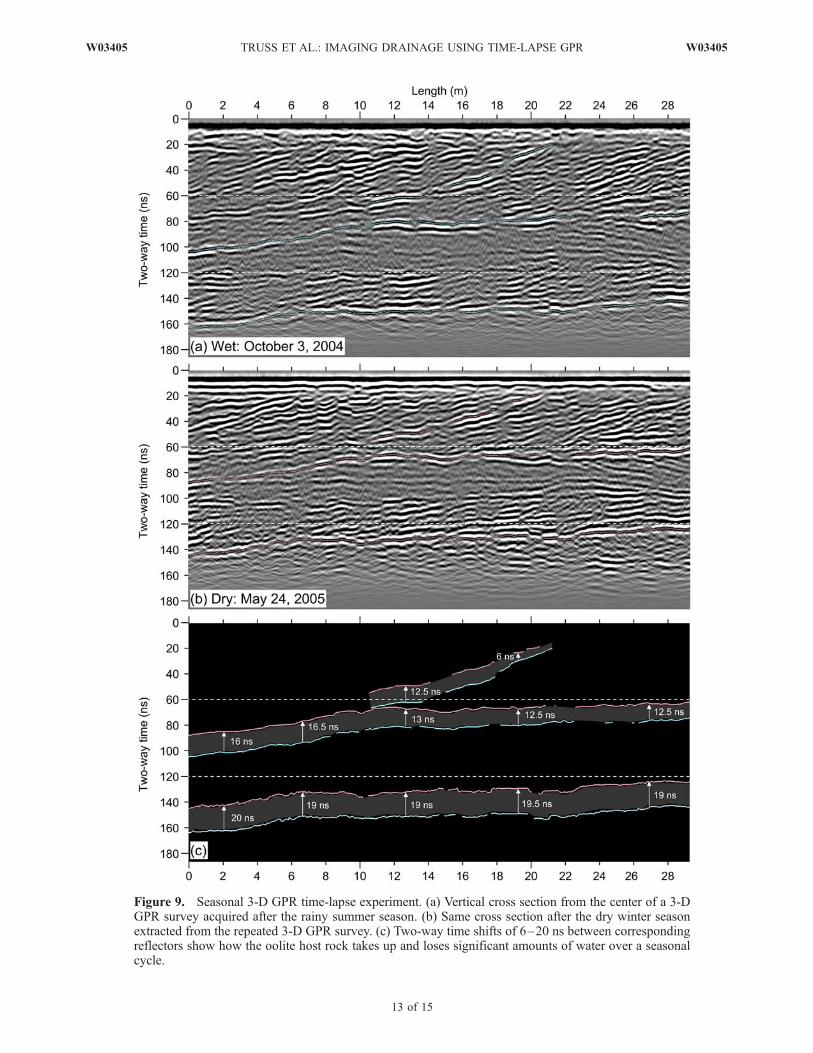
Figure 9. Seasonal 3-D GPR time-lapse experiment. (a) Vertical cross section from the center of a 3-DGPR survey acquired after the rainy summer season. (b) Same cross section after the dry winter seasonextracted from the repeated 3-D GPR survey. (c) Two-way time shifts of 6–20 ns between correspondingreflectors show how the oolite host rock takes up and loses significant amounts of water over a seasonalcycle.

W03405 TRUSS ET AL.: IMAGING DRAINAGE USING TIME-LAPSE GPR

13 of 15

W03405

compensation and 3-D migration. Velocity analysis usingdiffractions in the 3-D common-offset data indicated anaverage velocity of 0.075 m/ns for the October and0.085 m/ns for the May survey. Figure 9 shows time shiftsof 6–20 ns between corresponding reflections. Time shiftsare fairly constant along the profile but increase with depthas the radar waves travel longer distances causing a cumu-lative time stretch of the recorded GPR waveforms. Overallgeometry and configuration of reflection events remains thesame between seasons indicating an even distribution ofwater content change throughout the entire oolite rockvolume. This is in contrast to the localized and short-termchanges related to sinks shown earlier. It appears the vadosezone is taking up and losing significant amounts of water ona seasonal cycle like a sponge. As both bypass flow andlateral flow only affect part of the rock volume, the plugflow conceptual model driven by gravimetric and capillaryforces is most representative for the seasonal hydrologicvariation.

4. Conclusions

[37] The results show that a realistic vadose zone hydro-logic model of the field site in the Miami oolitic carbonatesshould incorporate all three initially proposed end-membermodels. Such a model including plug flow, lateral flow, andbypass flow can be used to characterize hydrologic con-ditions ranging from transient storm water drainage toseasonal water budget. Such wide temporal variability offlow models is likely to occur in other geohydrologicsettings where macropore and highly unstable flows occur.The time-lapse GPR method and survey strategy for thefield example shown in this paper is applicable to sitesdominated by karstic drainage and should be tested for othersites with suspected preferential flow paths. Rapid 2-Dtime-lapse GPR surveying before, during, and after rainfallprovides an initial assessment of the importance and loca-tion of preferential flow zones and an estimate of requiredsurvey repeat rates to adequately image the changes occur-ring in the subsurface related to flow. Full-resolution 3-Dtime-lapse imaging including 3-D migration to focus thediffractions then provides the geometry of preferentialflow paths and wetting fronts. Propagation rates can beestimated by comparing different stages of the infiltration.By inserting permanent survey markers in the ground,identical surveys can be acquired at field sites for long-term monitoring of annual and decadal changes of thevadose zone without disturbance of the natural flow paths.The key requirement for successful time-lapse imaging iscentimeter-precise positioning and reoccupation of GPRmeasurement locations. For field sites such precise andrapid imaging has become possible for the first time withthe recent development of a rotary laser-positioned GPRsystem.[38] After gaining this new qualitative insight into the

different drainage mechanisms operating in vadose zones,the next logical step is toward noninvasive quantification ofhydrological parameters by extraction of the GPR timeshifts caused by the changes of water content. Promisingapproaches in matching and warping of disparate 3-D datavolumes have already been developed in seismic [Rickettand Lumley, 2001] and medical imaging. Warp processingcross correlates corresponding GPR traces over a user-

selectable sliding time window and extracts the local timeshifts between reflection events from two repeat surveys.This last step will be essential to improve the resolution ofamplitude difference volumes resolving the flow pathswhere water content changes take place. In addition, the3-D time shift volume is directly related to time differencescaused by changes in water content. The time differencevolume can be inverted to water content changes usingpetrophysical relationships. The time-lapse GPR derivedpreferential flow path geometry and quantification ofchanges in water content inside the undisturbed vadosezone can then be used to develop and constrain the nextgeneration of numerical unsaturated flow models. Suchmodels will incorporate the realistic space-time variabilitycrucial for prediction of the hydrologic behavior of thevadose zone.

[39] Acknowledgments. This research was supported by the Univer-sity of Miami Innovative Teaching and Technology Initiative, the Compar-ative Sedimentology Laboratory, the donors of the American ChemicalSociety Petroleum Research Fund, and the National Science Foundation(grants 0323213 and 0440322). The University of Miami acknowledges thesupport of this research by Landmark Graphics Corporation via theLandmark University Software Grant Program. We thank Donald McNeilland Robert Ginsburg for sharing their expertise on the Miami limestone andfacilitating access to sites. Guillaume Koerner, Frank Despinois, and AdrianNeal helped with field work and figures. We gratefully acknowledge DavidBrown, city manager of Coral Gables, for granting permission to conductthis research in a city park. The paper was greatly improved with theexcellent ideas and the constructive suggestions from three anonymousreviewers, Associate Editor James R. Hunt, and Editor Scott W. Tyler.

ReferencesAnnan, A. P. (2003), Ground Penetrating Radar Principles, Proceduresand Applications, 278 pp., Sensors and Software, Mississauga, Ont.,Canada.

Aspiron, U., and T. Aigner (1997), Aquifer architecture analysisusing ground penetrating radar: Triassic and Quaternary examples(S. Germany), Environ. Geol., 31, 66–75.

Aspiron, U., and T. Aigner (1999), Towards realistic aquifer models: Three-dimensional georadar surveys of Quaternary gravel deltas (Singen Basin,SW Germany), Sediment. Geol., 129, 281–297.

Beres, M., P. Huggenberger, A. G. Green, and H. Horstmeyer (1999), Usingtwo- and three-dimensional georadar methods to characterize glacioflu-vial architecture, Sediment. Geol., 129, 1–24.

Best, J. L., P. J. Ashworth, C. S. Bristow, and J. Rodin (2003), Three-dimensional architecture of a large, mid-channel sand braid bar, JamunaRiver, Bangladesh, J. Sediment. Res., 73, 516–530.

Bevan, M. J., A. L. Endres, D. L. Rudolph, and G. Parkin (2003), The non-invasive characterization of pumping-induced dewatering using groundpenetrating radar, J. Hydrol., 281, 55–69.

Binley, A. M., P. Winship, R. Middleton, M. Pokar, and L. J. West (2001),High-resolution characterization of vadose zone dynamics using cross-borehole radar, Water Resour. Res., 37(11), 2639–2652.

Binley, A. M., G. Cassiani, R. Middleton, and P. Winship (2002), Vadosezone flow model parameterisation using cross-borehole radar and resis-tivity imaging, J. Hydrol., 267, 147–159.

Birken, R., and R. Versteeg (2000), Use of four-dimensional ground pene-trating radar and advanced visualization methods to determine subsurfacefluid migration, J. Appl. Geophys., 43, 215–226.

Brewster, M. L., and A. P. Annan (1994), Ground-penetrating radar mon-itoring of a controlled DNAPL release: 200 MHz radar, Geophysics, 59,1211–1221.

Calvert, R. (2005), 4D technology: Where are we, and where are wegoing?, Geophys. Prospect., 53, 161–171.

Corbeanu, R. M., K. Soegaard, R. B. Szerbiak, J. B. Thurmond, G. A.McMechan, D. Wang, S. Snelgrove, C. B. Forster, and A. Menitove(2001), Detailed internal architecture of a fluvial channel sandstonedetermined from outcrop, cores, and 3-D ground-penetrating radar:Example from the Middle Cretaceous Ferron sandstone, east-centralUtah, AAPG Bull., 85, 1583–1608.

Cunningham, K. J. (2004), Application of ground-penetrating radar, digitaloptical borehole images, and cores for characterization of porosity

14 of 15

W03405 TRUSS ET AL.: IMAGING DRAINAGE USING TIME-LAPSE GPR W03405

hydraulic conductivity and paleokarst in theBiscayne aquifer, southeasternFlorida, USA, J. Appl. Geophys., 55, 61–76.

Davis, J. L., and A. P. Annan (1989), Ground-penetrating radar for high-resolution mapping of soil and rock stratigraphy, Geophys. Prospect., 37,531–551.

Duerrast, H., and S. Siegesmund (1999), Correlation between rock fabricsand physical properties of carbonate reservoir rocks, Int. J. Earth Sci., 88,392–408.

Endres, A. L., W. P. Clement, and D. L. Rudolph (2000), Ground penetrat-ing radar imaging of an aquifer during a pumping test, Ground Water, 38,556–576.

Gloaguen, E., M. Chouteau, D. Marcotte, and R. Chapuis (2001), Estima-tion of hydraulic conductivity of an unconfined aquifer using cokrigingof GPR and hydrostratigraphic data, J. Appl. Geophys., 47, 135–152.

Grasmueck, M., and D. A. Viggiano (2005), First look at 4D GPR imagingof permeable zones around the borehole, in Expanded Abstracts of the75th Annual International Meeting: Society of Exploration Geophysics,pp. 2440–2443, Soc. of Explor. Geophys., Houston, Tex.

Grasmueck, M., and D. A. Viggiano (2007), Integration of ground-penetrating radar and laser position sensors for real time 3D data fusion,IEEE Trans. Geosci. Remote Sens., 45(1), 130–137.

Grasmueck, M., R. Weger, and H. Horstmeyer (2004), Three-dimensionalground-penetrating radar imaging of sedimentary structures, fractures,and archeological features at submeter resolution, Geology, 32, 933–936.

Grasmueck, M., R. Weger, and H. Horstmeyer (2005), Full-resolution 3-DGPR imaging, Geophysics, 70, K12–K19.

Greaves, R. J., D. P. Lesmes, J. M. Lee, and M. N. Toksoz (1996), Velocityvariations and water content estimated from multi-offset, ground-penetrating radar, Geophysics, 61, 683–695.

Grote, K., S. Hubbard, and Y. Rubin (2003), Field-scale estimationof volumetric water content using ground-penetrating radar groundwave techniques, Water Resour. Res., 39(11), 1321, doi:10.1029/2003WR002045.

Halley, R. B., and C. C. Evans (1983), The Miami Limestone: A Guide toSelected Outcrops and Their Interpretation (With a Discussion of Diag-enesis in the Formation), 65 pp., Miami Geol. Soc., Fla.

Halley, R. B., E. A. Shinn, J. H. Hudson, and B. H. Lidz (1977), Pleistocenebarrier bar seaward of ooid shoal complex near Miami, Florida, AAPGBull., 61, 519–526.

Heinz, J., and T. Aigner (2004), Three dimensional GPR analysis of variousQuaternary gravel-bed braided river deposits (southwestern Germany),Spec. Publ. Geol. Soc. London, 211, 99–110.

Hoffmeister, J. E., K. W. Stockman, and H. G. Multer (1967), Miami lime-stone of Florida and its recent Bahamian counterpart, Geol. Soc. Am.Bull., 78, 175–189.

Hubbard, S., K. Grote, and Y. Rubin (2002), Mapping the volumetric soilwater content of a California vineyard using high-frequency GPR groundwave data, Leading Edge Explor., 21, 552–559.

Huisman, J. A., S. S. Hubbard, J. D. Redman, and A. P. Annan (2003),Measuring soil water content with ground penetrating radar: A review,Vadose Zone J., 2, 476–491.

Lambot, S., M. Antoine, M. Vanclooster, and E. C. Slob (2006), Effect ofsoil roughness on the inversion of off-ground monostatic GPR signal fornoninvasive quantification of soil properties, Water Resour. Res., 42,W03403, doi:10.1029/2005WR004416.

Neal, A. (2004), Ground-penetrating radar and its use in sedimentology:Principles, problems and progress, Earth Sci. Rev., 66, 261–330.

Nobes, D. C., H. M. Jol, and H. Rother (2004), Radar ‘‘lensing’’ by a smallriver: Can a layer of surface water improve the signal?, in GPR 2004:Proceedings of the Tenth International Conference, pp. 539–542, DelftUniv. of Technol., Delft, Netherlands.

Rickett, J., and D. E. Lumley (2001), Cross-equalization data processing fortime-lapse seismic reservoir monitoring: A case study from the Gulf ofMexico, Geophysics, 66, 1015–1025.

Smith, D. G., and H. M. Jol (1992), Ground-penetrating radar investigationof a Lake Bonneville delta, Provo level, Bingham City, Utah, Geology,20, 1083–1086.

Tidwell, V. C., and J. L. Wilson (1997), Laboratory method for investigat-ing permeability upscaling, Water Resour. Res., 33, 1607–1616.

Topp, G. C., J. L. Davis, and A. P. Annan (1980), Electromagnetic deter-mination of soil water content: Measurements in coaxial transmissionlines, Water Resour. Res., 16, 574–582.

Trinks, I., D. Wachsmuth, and H. Stumpel (2001), Monitoring water flow inthe unsaturated zone using georadar, First Break, 19, 679–684.

Truss, S. W. (2004), Characterisation of sedimentary structure and hydraulicbehaviour within the unsaturated zone of the Triassic Sherwood Sand-stone aquifer in north east England, Ph.D. thesis, Univ. of Leeds, Leeds,U.K.

Tsoflias, P. G., T. Halihan, and J. M. Sharp, Jr. (2001), Monitoring pumpingtest response in a fractured aquifer using ground-penetrating radar, WaterResour. Res., 37, 1221–1229.

Van Dam, R. L., and W. Schlager (2000), Identifying causes of ground-penetrating radar reflections using time-domain reflectometry and sedi-mentological analyses, Sedimentology, 47, 435–449.

Van Overmeeren, R. A., S. V. Sariowan, and J. C. Gehrels (1997), Groundpenetrating radar for determining volumetric soil water content: Resultsof comparative measurements at two sites, J. Hydrol., 197, 316–338.

Versteeg, R. (2002), Near-real time imaging of subsurface processes usinggeophysics, in Expanded Abstracts of the 72nd Annual InternationalMeeting: Society of Exploration Geophysics, pp. 1500–1503, Soc. ofExplor. Geophys., Salt Lake City, Utah.

Yilmaz, O. (2000), Seismic Data Analysis, Soc. of Explor. Geophys., Tulsa,Okla.

����������������������������M. Grasmueck (corresponding author) and D. A. Viggiano, Division of

Marine Geology and Geophysics, Rosenstiel School of Marine andAtmospheric Science, University of Miami, 4600 Rickenbacker Causeway,Miami, FL 33149, USA. ([email protected])

S. Truss, School of Earth and Environment, University of Leeds, Leeds,LS2 9JT, UK.

S. Vega, Petroleum Institute, P.O. Box 2533, Abu Dhabi, UAE.

W03405 TRUSS ET AL.: IMAGING DRAINAGE USING TIME-LAPSE GPR

15 of 15

W03405