Imaging by integrating stitched spectrograms

Imaging by integrating stitched spectrograms

Carson Teale,1,*

Dan Adams,1,2

Margaret Murnane,1 Henry Kapteyn,

1

and Daniel J. Kane3

1JILA, University of Colorado at Boulder, 440 UCB, Boulder, Colorado 80309-0440, USA 2Kapteyn-Murnane Laboratories, 1855 South 57th Court, Boulder, Colorado 80301, USA

3Mesa Photonics, LLC, 1550 Pacheco St., Santa Fe, New Mexico 87505, USA *[email protected]

Abstract: A new diffractive imaging technique called Imaging By

Integrating Stitched Spectrograms (IBISS) is presented. Both the data

collection and phase retrieval algorithm used in IBISS are direct extensions

of frequency resolved optical gating to higher dimensions. Data collection

involves capturing an array of diffraction patterns generated by scanning a

sample across a coherent beam of light. Phase retrieval is performed using

the Principal Components Generalized Projections Algorithm (PCGPA) by

reducing the four dimensional data set of images to two remapped two-

dimensional sets. The technique is successfully demonstrated using a

Helium Neon laser to image a 350μm wide sample with 12μm resolution.

©2013 Optical Society of America

OCIS codes: (110.1455) Blind deconvolution; (070.0070) Fourier optics and signal processing;

(180.5810) Scanning microscopy; (110.0180) Microscopy.

References and links

1. D. Sayre, “Some implications of a theorem due to Shannon,” Acta Crystallogr. A, 843 (1952).

2. J. Miao, P. Charalambous, J. Kirz, and D. Sayre, “Extending the methodology of X-ray crystallography to allow imaging of micrometre-sized non-crystalline specimens,” Nature 400(6742), 342–344 (1999).

3. K. Giewekemeyer, P. Thibault, S. Kalbfleisch, A. Beerlink, C. M. Kewish, M. Dierolf, F. Pfeiffer, and T. Salditt,

“Quantitative biological imaging by ptychographic x-ray diffraction microscopy,” Proc. Natl. Acad. Sci. U.S.A. 107(2), 529–534 (2010).

4. P. Thibault, V. Elser, C. Jacobsen, D. Shapiro, and D. Sayre, “Reconstruction of a yeast cell from X-ray

diffraction data,” Acta Crystallogr. A 62(4), 248–261 (2006).

5. C. A. Larabell and K. A. Nugent, “Imaging cellular architecture with X-rays,” Curr. Opin. Struct. Biol. 20(5),

623–631 (2010).

6. F. Berenguer de la Cuesta, M. P. E. Wenger, R. J. Bean, L. Bozec, M. A. Horton, and I. K. Robinson, “Coherent X-ray diffraction from collagenous soft tissues,” Proc. Natl. Acad. Sci. U.S.A. 106(36), 15297–15301 (2009).

7. J. Nelson, X. Huang, J. Steinbrener, D. Shapiro, J. Kirz, S. Marchesini, A. M. A. M. Neiman, J. J. J. J. Turner, and C. Jacobsen, “High-resolution x-ray diffraction microscopy of specifically labeled yeast cells,” Proc. Natl.

Acad. Sci. U.S.A. 107(16), 7235–7239 (2010).

8. Y. Sung, W. Choi, C. Fang-Yen, K. Badizadegan, R. R. Dasari, and M. S. Feld, “Optical diffraction tomography for high resolution live cell imaging,” Opt. Express 17(1), 266–277 (2009).

9. R. L. Sandberg, D. A. Raymondson, C. La-O-Vorakiat, A. Paul, K. S. Raines, J. Miao, M. M. Murnane, H. C.

Kapteyn, and W. F. Schlotter, “Tabletop soft-x-ray Fourier transform holography with 50 nm resolution,” Opt. Lett. 34(11), 1618–1620 (2009).

10. H. Jiang, C. Song, C. C. Chen, R. Xu, K. S. Raines, B. P. Fahimian, C. H. Lu, T. K. Lee, A. Nakashima, J.

Urano, T. Ishikawa, F. Tamanoi, and J. Miao, “Quantitative 3D imaging of whole, unstained cells by using X-ray diffraction microscopy,” Proc. Natl. Acad. Sci. U.S.A. 107(25), 11234–11239 (2010).

11. Y. Nishino, Y. Takahashi, N. Imamoto, T. Ishikawa, and K. Maeshima, “Three-dimensional visualization of a

human chromosome using coherent x-ray diffraction,” Phys. Rev. Lett. 102(1), 018101 (2009). 12. B. Abbey, K. A. Nugent, G. J. Williams, J. N. Clark, A. G. Peele, M. Pfeifer, M. de Jonge, and I. McNulty,

“Keyhole coherent diffractive imaging,” Nat. Phys. 4(5), 394–398 (2008).

13. H. M. Quiney, G. Peele, Z. Cai, D. Paterson, and K. A. Nugent, “Diffractive imaging of highly focused X-ray fields,” Nat. Phys. 2(2), 101–104 (2006).

14. G. Williams, H. Quiney, B. Dhal, C. Tran, K. Nugent, A. Peele, D. Paterson, and M. de Jonge, “Fresnel Coherent

Diffractive Imaging,” Phys. Rev. Lett. 97(2), 025506 (2006). 15. D. J. Vine, G. J. Williams, B. Abbey, M. Pfeifer, J. N. Clark, M. D. de Jonge, I. McNulty, G. Peele, and K.

Nugent, “Ptychographic Fresnel coherent diffractive imaging,” Phys. Rev. A 80(6), 063823 (2009).

#181558 - $15.00 USD Received 11 Dec 2012; revised 13 Feb 2013; accepted 14 Feb 2013; published 11 Mar 2013(C) 2013 OSA 25 March 2013 / Vol. 21, No. 6 / OPTICS EXPRESS 6783

16. G. Williams, H. Quiney, B. Dahl, C. Tran, A. G. Peele, K. A. Nugent, M. D. De Jonge, and D. Paterson, “Curved

beam coherent diffractive imaging,” Thin Solid Films 515(14), 5553–5556 (2007). 17. T. Harada, M. Nakasuji, T. Kimura, T. Watanabe, H. Kinoshita, and Y. Nagata, “Imaging of extreme-ultraviolet

mask patterns using coherent extreme-ultraviolet scatterometry microscope based on coherent diffraction

imaging,” J. Vac. Sci. Technol. B 29(6), 06F503 (2011). 18. T. Harada, J. Kishimoto, T. Watanabe, H. Kinoshita, and D. G. Lee, “Mask observation results using a coherent

extreme ultraviolet scattering microscope at NewSUBARU,” J. Vac. Sci. Technol. B 27(6), 3203 (2009).

19. D. F. Gardner, B. Zhang, M. D. Seaberg, L. S. Martin, D. E. Adams, F. Salmassi, E. Gullikson, H. Kapteyn, and M. Murnane, “High numerical aperture reflection mode coherent diffraction microscopy using off-axis apertured

illumination,” Opt. Express 20(17), 19050–19059 (2012).

20. M. Dierolf, O. Bunk, S. Kynde, P. Thibault, I. Johnson, A. Menzel, K. Jefimovs, C. David, O. Marti, and F. Pfeiffer, “Ptychography & lensless x ray imaging,” Europhys. News 39(1), 22–24 (2008).

21. P. Thibault, M. Dierolf, O. Bunk, A. Menzel, and F. Pfeiffer, “Probe retrieval in ptychographic coherent

diffractive imaging,” Ultramicroscopy 109(4), 338–343 (2009). 22. D. Kane, “Principal components generalized projections : a review [ Invited ],” J. Opt. Soc. Am. B 25(6), A120–

A130 (2008).

23. R. Trebino and D. Kane, “Using phase retrieval to measure the intensity and phase of ultrashort pulses: frequency-resolved optical gating,” J. Opt. Soc. Am. 10(5), 1101 (1993).

24. H. Stark, Image Recovery : Theory and Application (Academic Press, 1986).

25. R. Trebino, Frequency-resolved Optical Gating: The Measurement of Ultrashort Laser Pulses (Kluwer

Academic, 2000).

26. K. DeLong, R. Trebino, J. Hunter, and W. White, “Frequency-resolved optical gating with the use of second-

harmonic generation,” J. Opt. Soc. Am. B 11(11), 2206–2215 (1994). 27. D. Kane, “Principal components generalized projections: a review,” J. Opt. Soc. Am. B 25(6), A120–A132

(2008).

28. K. W. DeLong, R. Trebino, and W. E. White, “Simultaneous recovery of two ultrashort laser pulses from a single spectrogram,” J. Opt. Soc. Am. B 12(12), 2463 (1995).

29. D. J. Kane, G. Rodriguez, A. Taylor, and T. S. Clement, “Simultaneous measurement of two ultrashort laser pulses from a single spectrogram in a single shot,” J. Opt. Soc. Am. B 14(4), 935–943 (1997).

30. B. C. McCallum and J. M. Rodenburg, “Simultaneous reconstruction of object and aperture functions from

multiple far-field intensity measurements,” J. Opt. Soc. Am. 10(2), 231 (1993).

1. Introduction

The concept of phase retrieval from an oversampled, coherent scatter pattern was first

suggested by Sayre in 1952 [1], and demonstrated experimentally for the first time in 1999 by

Miao et. al. [2] in the original coherent diffraction imaging (CDI) implementation. In this

version of CDI, a plane wave scatters from an isolated sample and is recorded in the far-field

using a square law detector. In this regime, the diffraction pattern is proportional to the

Fourier transform of the scattering electronic potential; however, because complex wave-

propagation information is lost during this measurement, an iterative algorithm must be used

to solve for the missing diffracted phases while concurrently reconstructing an image of the

specimen. The original CDI algorithms proceed by making use of two constraints: 1) the

measured diffracted amplitudes, and 2), the condition that the specimen is completely isolated

(i.e. the entire finite size object is illuminated by the wave). The strength of this approach to

CDI lies in the fact that it uses the amplitude of just one diffraction pattern, reducing data

collection times and radiation dose. In most cases, the diffraction pattern is digitally sampled

at a frequency very near the minimum necessary for unique phase retrieval. Because of this,

conventional phase retrieval algorithms typically require a very large number of iterations and

unique convergence is not always guaranteed.

In recent years, CDI techniques have greatly improved, enabling very high resolution 2D

and 3D imaging of biological and materials samples using coherent light sources [3–11]. In

order to alleviate constraints and enhance convergence properties of CDI, several new

variants have been implemented with differing strengths and weaknesses. Major advances

include keyhole-CDI and other curved wave-front variants [12–16], where the light

illumination (rather than the sample) is truncated to satisfy the isolation constraint, or

apertured illumination-CDI (AI-CDI), where an aperture is imaged directly onto the sample

[17–19]. Another very successful technique that isolates the impinging wave rather than the

specimen is ptychography [15,20,21]. In this approach, a well-characterized and localized


coherent beam scatters from the specimen and several far-field patterns are collected from

overlapping regions of the sample. The reconstruction algorithm then attempts to produce an

object whose Fourier modulus is consistent with all of the collected scatter patterns. In

ptychography, the wave truncation is achieved by means of a pinhole placed very near the

sample being scanned.

Here we present Imaging by Integrating Stitched Spectrograms (IBISS) as a novel

solution to phase retrieval. IBISS is similar to ptychography in that several diffraction

patterns are collected containing overlapping, redundant information, which helps ensure

unique and rapid convergence. However, in IBISS, the extra, overlapping data also provides

enough information to simultaneously reconstruct the amplitude and phase of the beam, in

addition to the sample, without the need for a priori information.

2. Theory

IBISS is a direct extension of conventional Frequency Resolved Optical Gating (FROG)

[22,23] techniques to diffractive imaging. In a FROG measurement, the amplitude and phase

of an ultrashort pulse are recovered by converting an unsolvable one-dimensional

deconvolution into a solvable two-dimensional deconvolution. To do this, an ultrashort pulse

is split into two paths, which are delayed with respect to each other. These two paths are then

recombined in a nonlinear material that acts as a multiplier to gate portions of the pulse by the

delayed pulse replica. The spectrum of the resulting signal is then recorded for a series of

time delays. If a second harmonic generating (SHG) crystal is used, then the resulting

nonlinear signal will be directly proportional to the product of the pulse with the delayed

pulse. The PCGP algorithm can be used to retrieve the amplitude and the phase of the pulse

using the spectrogram data. The PCGP algorithm is not constrained to inverting spectrograms

generated using the pulse to gate itself; it is capable of inverting spectrograms generated by

an unknown pulse and an unknown gating function. However, because the PCGP algorithm is

a generalized projections algorithm, it does not form a projection onto a convex set, and is not

guaranteed to converge. In spite of this, generalized projections algorithms are still expected

to work well [24]. For a general discussion and broad overview of FROG, please see [25] and

the references therein.

The data collection process for IBISS is directly analogous to that of FROG. Rather than

gating a one-dimensional pulse in time, a spatial, two-dimensional beam is gated by a two

dimensional sample which is translated in a plane perpendicular to the beam. In the same way

that the signal in FROG is the product of the pulse and the delayed pulse, the signal

immediately after the sample in IBISS is the product of the beam and translated sample. The

two dimensional spectrum of this signal is recorded by placing a camera in the far-field of the

sample or, more practically, at the focus of a Fourier transform lens, which is placed

immediately after the sample. Instead of generating a two-dimensional data set composed of

one dimensional vectors (representing the spectrum of the signal at different delay times), a

four dimensional data set composed of two-dimensional spatial spectra at different scan

positions is recorded.

The PCGP algorithm can be used to recover the amplitude and phase of the sample and

beam in almost exactly the same way that it is used to recover the shape of a pulse and gate in

FROG [26]. When used to invert a FROG trace, the PCGP algorithm finds the best

approximation for the two dimensional spectrogram that can be formed by remapping the

outer product of a one dimensional pulse vector and a one dimensional gate vector. In IBISS,

the PCGP algorithm finds the best approximation for the four-dimensional data that can be

formed by mapping the outer product of two, two-dimensional matrices (images) representing

the sample and the beam. To simplify programming of the PCGP algorithm for this imaging

application, the four dimensional data set is remapped to a two-dimensional matrix, and the

two-dimensional images of the sample and beam are remapped to vectors.


The beam and sample being measured in IBISS will be represented as follows:

( , )beamE x y and ( , )sample x X y YG where X and Y represent the displacement of the sample.

The signal immediately after the sample is

, , , ( , ) ( , )sig beam sampleE x y X Y E x y G x X y Y (1)

and the spectrum of this signal is

( ), , , ( , , , ) x yi xf yf

spec x y sigE f f X Y E x y X Y e dxdy

∬ (2)

The camera records the intensity of the spectrum at each scan position (absolute value

squared of Eq. (2)):

2

( ), , , ( , , , ) x yi xf yf

spec x y sigI f f X Y E x y X Y e dxdy

∬ (3)

The PCGP algorithm uses Eqs. (1) and (3) as constraints. Equation (1), which is applied in the

object domain, is used to obtain the next guess for the beam and sample as well as to

construct the guess for the signal immediately after the sample. The constraint from Eq. (3),

which is applied in the frequency domain, forces the amplitude of the guess for the

spectrogram to be equal to the measured amplitude. Before this constraint is imposed, the

error can be estimated in an RMS fashion, by summing the square of the difference between

the two amplitudes and taking the square root of the sum.

In the most general case, the inversion algorithm begins with a random guess for the

amplitude and phase of the beam and the sample and then uses Eq. (1) to generate a guess for

the signal field, ' , , , .sigE x y X Y This guess is then Fourier transformed along the x and y

directions to obtain a guess for the collection of spectra:

' , , ,' , , , ' , , , x yi f f X Y

spec x y spec x yE f f X Y I f f X Y e

(4)

At this point the amplitudes in Eq. (4) are replaced with the measured amplitudes,

, , , .spec x yI f f X Y The result, ' , , ,, , , x yi f f X Y

spec x yI f f X Y e

is used to obtain the next

guess for the beam and sample. The following is a more detailed description of how this is

accomplished in the PCGP algorithm.

We will represent the discretized beam and sample as two-dimensional matrices:

1,1 1, 1,1 1,

,1 , ,1 ,

N N

beam sample

N N N N N N

E E G G

E G

E E G G

(5)

The algorithm computes the outer product of these matrices by first linearizing the N x N

matrices of Eq. (5) to 1 x N2 vectors:


1,1 ,1 1,2 ,2 1, ,

1,1 ,1 1,2 ,2 1, ,

1,1 1,1 1,1 2,1 1,1 ,1 1,1 ,

2,1 1,1 2,1 2,1 2,1 ,1 2,1 ,

3,1 1,1 3,1 2,1 3,1 ,1 3,1 ,

lin N N N N N

lin N N N N N

N N N

N N N

N N N

T

outer lin lin

E E E E E E E

G G G G G G G

E G E G E G E G

E G E G E G E G

E G E G E G E G

E E G

,1 1,1 ,1 2,1 ,1 ,1 ,1 ,

1,2 1,1 1,2 2,1 1,2 ,1 1,2 ,

, 1,1 , 2,1 , ,1 , ,

N N N N N N N

N N N

N N N N N N N N N N N

E G E G E G E G

E G E G E G E G

E G E G E G E G

(6)

Since this outer product contains every possible combination of the product of an element of

E with that of G, there is a one to one mapping from the outer product to the object domain

signal, Esig. The object domain signal is produced by first rotating the elements in the rows of

the outer product matrix given in Eq. (6) to the left by the row number minus one. The

resulting matrix is shown below:

1,1 1,1 1,1 2,1 1,1 ,1 1,1 ,

2,1 2,1 2,1 3,1 2,1 1,2 2,1 1,1

3,1 3,1 3,1 4,1 3,1 2,2 3,1 2,1

,1 ,1 ,1 1,2 ,1 1,2 ,1 1,1

1,2 1,2 1,2 2,2 1,2 1,,2 2

,

,1

,

N N N

N N

rot

N

N N N

N

N N

N N N N

E G E G E G E G

E G E G E G E G

E G E G E G E G

EE G E G E G E G

E G E G E G E G

E G

, 1,1 , 1,1 , 1,N N N N N N N N NE G E G E G

(7)

Each column of the matrix in Eq. (7) represents a linearized object domain signal at a

particular scan position. The first N columns are the object domain signals which are formed

by shifting the sample one through N steps in the Y direction and 0 steps in the X direction.

The next N columns are the result of shifting the sample one through N steps in the Y

direction and 1 step in the X direction and so on. These columns are reshaped into N by N

sub-matrices composing the entire N2 x N

2 matrix.

1,1 1,1 1,2 1,2 1, 1, 1,1 1,2 1,2 1,3 1, 1,1 1,1 1,3 1, 1, 1

2,1 2,1 2,2 2,2 2, 2, 2,1 2,2 2,2 2,3 2, 2,1 2,1 2,3 2, 2, 1

,1 ,1 ,2 ,2

0 ...

0

...

N N N N N

N N N N N

N N N N

sig

E G E G E G E G E G E G E G E G


E G E G E

E

X X X X

Y

Y X

Y

, , ,1 ,2 ,2 ,3 , ,1 ,1 ,3 , , 1

1,1 2,1 1,2 2,2 1, 2, 1,1 2,2 1,2 2,3 1, 2,1 1,1 2,3 1, 2, 1

2,1 3,1 2,2 3,2 2, 3, 2,1 3,2 2,2 3,3 2, 3,1 2,1 3,3 2, 3, 1

N N N N N N N N N N N N N N N N N

N N N N N

N N N N N

G E G E G E G E G E G



,1 1,1 ,2 1,2 , 1, ,1 1,2 ,2 1,3 , 1,1 ,1 1,3 , 1, 1

1,1 3,1 1,2 3,2 1, 3, 1,1 3,2 1,2 3,3 1, 3,1 1,1 3,3 1, 3, 1

,1 1,1 ,2 1,2 , 1,

N N N N N N N N N N N N N

N N N N N

N N N N N N N N



E G E G E G E

,1 1,2 ,2 1,3 , 1,1 ,1 1,3 , 1, 1N N N N N N N N N N N N NG E G E G E G E G

(8)


Now the first N x N elements in Eq. (8) are the beam multiplied by the un-shifted sample

(X = 0 and Y = 0). The sub-matrix labeled X = -ΔX, Y = 0 is the beam multiplied by the

sample shifted one step to the left in the X direction. The matrix labeled X = 0 and Y = -ΔX is

the beam multiplied by the sample shifted one step up in the Y direction. Together the

collection of sub-matrices represents the product , ( , )beam sampleE x y G x X y Y for all

combinations of , Δ , Δ 1, , Δ 1 .2 2 2

N N NX Y X X X

Thus, there exists a

straightforward transformation between the outer product and the object domain IBISS signal

and vice versa. To obtain the IBISS spectrogram from the object domain signal, each sub-

matrix is Fourier transformed.

The phase retrieval process uses this transformation to iterate back and forth between the

object and frequency domains, imposing constraints in each. After beginning with a random

guess for the phase and amplitude of both the sample and beam, these matrices are linearized

and their outer product computed. Using the row shifting and sub-matrix reshaping procedure

described previously, the object domain IBISS signal is produced. The spectrogram is formed

by taking the two-dimensional Fourier transform of each sub-matrix of the object domain

signal. At this point, the amplitude of the spectrogram is replaced with the square root of the

measured spectrogram intensity data but the phase of the guess is retained. The result is

inverse Fourier transformed back to the object domain. The row shifting procedure is reversed

to obtain what will be called an outer product form matrix. The result is not a true outer

product (Rank 1 matrix) unless the guess for the sample and beam were correct. The principal

components of the outer product form matrix can be found by performing a singular value

decomposition or using the power method in exactly the same way as is done using the PCGP

algorithm for inverting a two dimensional FROG trace [27]. These principal components

represent the two vectors with the largest weighting factor when the outer product form

matrix is decomposed into a superposition of outer products. The outer product of the

principal component vectors is the best rank 1 approximation of the outer product form matrix

in the least squares sense. The principal components, which form a generalized projection, are

selected as the next best guess for the beam and the sample. This process is repeated until the

error between the guess for the spectrogram amplitude and the measured spectrogram

amplitude is sufficiently small. The possible ambiguities of the resulting reconstruction are

the addition of a constant and linear phase to the sample and beam matrices (the same

ambiguities that exist for FROG) [28,29].

This algorithm inherently requires that the sample either be isolated or periodic. This

constraint arises because of the way the algorithm generates the guess for Esig (Eq. (8)) from

the guess for the beam and sample matrices. From Eq. (8), it can be seen that in each sub-

matrix, the sample matrix (Gsample) has been circularly shifted, that is, any elements that are

shifted beyond the edge of the matrix are wrapped around to the other side. This method

generates an accurate representation of Esig when the sample being imaged is isolated

(surrounded by a completely opaque material) because the elements of Gsample that get

wrapped around are either zeros or multiplied by zeros in Ebeam. This circular shifting also

works for imaging periodic samples since the elements of the sample that are wrapped around

exactly match the next part of the sample being illuminated as long as the scan distance is

some multiple of the sample’s period.

Another limitation of this imaging technique arises due to the rapid increase of the

computation time with input size. Since the pixel resolution is determined by the number of

scan positions, it is desirable to record as many diffraction patterns as possible. However, the

runtime of the algorithm is 4 2log ,O N N where N is the number of scan positions in one

dimension.


3. Methods

In our experimental setup (see Fig. 1), a Helium-Neon laser was used to illuminate the sample

and the diffraction pattern was collected by a CCD. A spatial filter was used to produce an

ideal, Gaussian, laser beam intensity cross section. The spatial filter consisted of a 6 cm lens

used to focus the laser beam through a 25µm circular pinhole (1.). A second 6 cm lens was

placed after the pinhole to collimate the beam. Since the IBISS algorithm can reconstruct the

amplitude and phase of both the sample and the beam, the exact shape of the beam incident

on the sample is not critical. In order to emphasize this point, a 25µm by 25µm square

pinhole (2.) was imaged onto the sample. The sample (3.) was placed on a motorized stage

that moved in a plane perpendicular to the beam propagation direction (with 1 µm step size).

A Fourier transform lens (L3), with a focal length of 10 cm, was placed immediately after the

sample. The camera was placed at the focus of the Fourier transform lens (4.) and was

mounted on a translation stage which moves in the direction of the beam path so that its

position could be precisely controlled. The camera is a windowless, USB controlled, CMOS

camera with 1024 by 1280 pixels, each of width 5.2µm.

The sample, shown in Fig. 1(b), was a thin (12.7um), opaque, stainless steel sheet with an

L shaped hole that was cut using a focused laser. The longer leg of the L is about 350µm

while the shorter leg is about 250µm. Data was acquired by performing a line-by-line scan of

the sample across all X and Y positions. At each position, the program records a series of

images at different exposure times, which are then combined to form a final, high dynamic

range (HDR) image.

The bit depth of the camera is 8 bits (corresponding to 256 different intensity values). In

order to take advantage of this entire range, it would be necessary to pick an exposure time

such that the brightest pixel had the maximum value, but was still not saturated. To increase

the effective bit depth, multiple pictures are captured at different exposure times. The smallest

exposure time has no saturated data while larger exposure times have more and more

saturated data. These images are then combined into one, HDR image by replacing the

saturated data in one picture with a properly scaled set of unsaturated data from a picture

taken at a shorter exposure time. This process has the effect of increasing the bit depth so that

a much wider range of intensity values can be recorded and therefore finer details of the

diffraction pattern can be used during reconstruction of the sample.

Fig. 1. (a) Schematic of experiment. (b) Standard, reflection microscope image of the sample. (c) Image of the beam incident on the sample. (1. Spatial filter pinhole. L1. Collimating lens. 2.

Square pinhole that is imaged to the sample by an imaging lens L2. 3. Sample plane. L3 forces

the diffracted light to the far-field and detector plane 4.)


The PCGP algorithm requires that the number of different scan positions be equal to the

number of pixels in each image. A huge number of pictures would be required if the full

resolution of the camera (1280x1024) were used. Therefore the images are first cropped

square and then binned to 32x32 or 64x64 pixels, since larger resolutions would result in

extremely long reconstruction run times. Furthermore, the pixel resolution of the

reconstructed images is equal to the number of scan positions since the collection of

diffraction patterns is the same dimensionality as the outer product of the sample and beam

matrices. So if 64x64 diffraction patterns are recorded, each with 64x64 pixels, then the full

collection of diffraction patterns has a size of 642x64

2. Since this is also the dimensionality of

the outer product of the sample and beam matrices, the size of those matrices must be 64x64.

The PCGP algorithm requires that the step size of the scanned sample (dX) be equal to the

sampling period of the beam and sample (dx). Since x and y, the spatial coordinates of the

beam and sample, are Fourier transform pairs with fx and fy, the spatial frequencies associated

with the diffraction patterns, it must be the case that 1

xmax

dxf

and 1

.ymax

dyf

In the

paraxial limit, the value of fx can be estimated by cx

xf

z where xc is the distance from the

center of the diffraction pattern, λ is the wavelength, and z is the focal length of the Fourier

transform lens. Combining these equations, we get

1

xmax cmax

z zdX dx dY

f x pN

(9)

where p is the effective pixel size (5.2µm multiplied by the binning factor of either 16 or 32)

and N is the number of scan positions. The focal length of the Fourier transform lens was

chosen to be 10cm. With these parameters and a binning factor of 16, Eq. (9) gives a required

step size of 11.88µm. The full scan distance, which limits the size of the sample to be imaged,

is just the step size multiplied by the number of scan positions.

The diffraction pattern must be sampled at a frequency greater than or equal to the

Nyquist frequency, which is twice the highest frequency component of the sample being

illuminated. The period of the highest frequency component of the object will be the

reciprocal of half of its largest feature size:

2

xdfD

(10)

where the size of the sample is D. To convert this spatial frequency into detector coordinates,

we again use the paraxial approximation:

x

xf

z (11)

The result of substituting Eq. (11) into Eq. (10) is:

2 z

dxD

(12)

This is the period of the highest frequency component of the diffraction pattern on the

camera. The Nyquist frequency is twice the value of the highest frequency component (twice

the reciprocal of Eq. (12):

N

Df

z (13)


For the L shaped sample that was imaged, D (the size of the sample) = 350µm, and Eq. (13)

gives a value of 5.53x103 m

1 for the Nyquist frequency (fN). The actual sampling rate was

1/(2p) = 6.01x103m

1 which is greater than fN.

4. Results

A data set was collected by imaging a 25µm by 25 µm square pinhole onto the “L- shaped”

sample with a magnification of two. Images of the beam and sample, as well as the collection

of diffraction patterns recorded during a full scan across the sample, are shown in Fig. 2. The

image of the beam shown in Fig. 2 was captured by removing the sample and placing another

camera in exactly the same plane in order to record the shape of the beam at the sample. This

camera was then removed, the sample was replaced, and the data set was recorded with a total

of 64x64 diffraction patterns captured. Each image was taken with the sample at a different

position relative to the beam and was binned down to a size of 64x64 pixels. Figure 2(a) and

2(b) show images of the sample and laser illumination beam respectively. Figure 2(c) shows a

concatenation of all the diffraction patterns, while Fig. 2(d) shows a zoomed-in view of a few

individual diffraction patterns.

Fig. 2. Data Set: (a) microscope image of sample, (b) image of beam (c) 64x64 diffraction

patterns (each 64x64 pixels) at different scan positions, concatenated together (inset shows the

image generated by binning each diffraction pattern to one pixel), (d) zoomed in on a few diffraction patterns

Figure 3 plots the reconstructions of the amplitude and phase of both the sample and beam

after running the algorithm for 100 iterations, which required approximately 30 minutes on a

high powered cluster running Matlab code. The reconstructed amplitudes of the beam and

sample were found to be in excellent agreement with the measured profiles (insets in Fig. 3(a)

and 3(c)). Figure 4 shows the RMS error between the amplitude of the measured diffraction

patterns and the guess for the diffraction patterns, at each iteration. After about sixty iterations

the error no longer changes significantly, indicating that the algorithm has converged. As

expected, the IBISS spectrogram resembles the object and can be used to generate a first

guess for the amplitude in the algorithm. A smoothed guess for the amplitude is generated by

binning each sub-matrix (diffraction pattern) to one pixel, and is shown in the inset of Fig.

2(c).


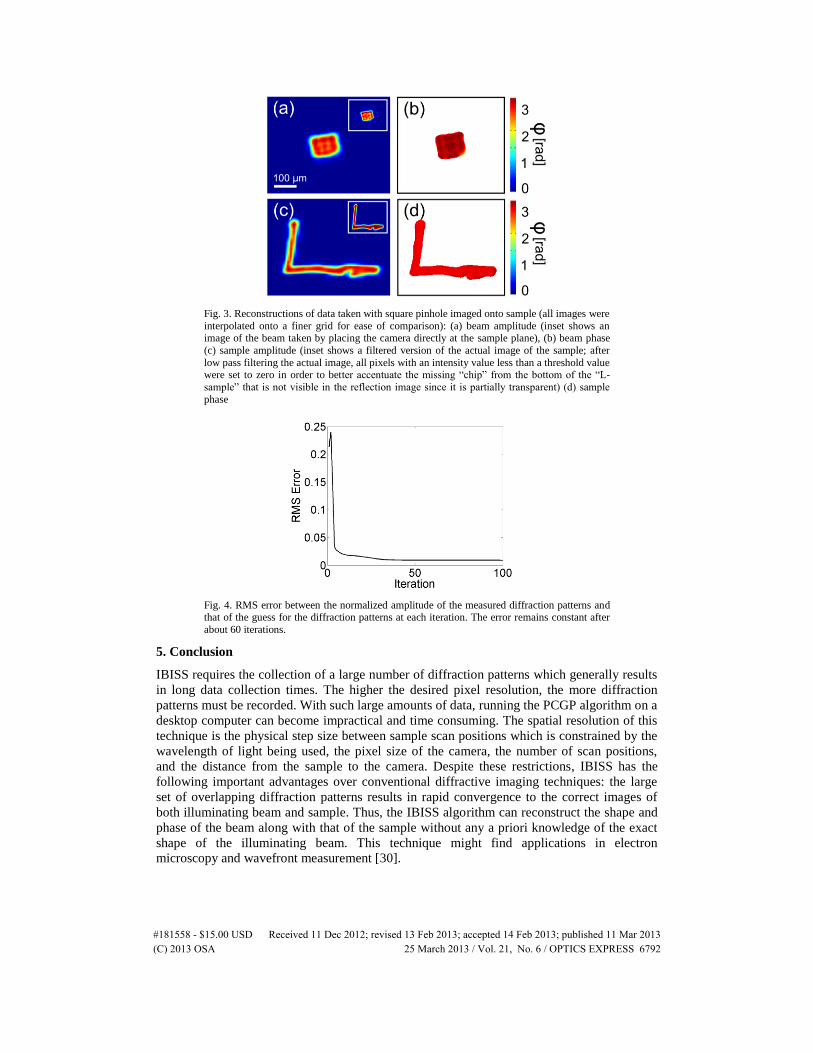
Fig. 3. Reconstructions of data taken with square pinhole imaged onto sample (all images were

interpolated onto a finer grid for ease of comparison): (a) beam amplitude (inset shows an image of the beam taken by placing the camera directly at the sample plane), (b) beam phase

(c) sample amplitude (inset shows a filtered version of the actual image of the sample; after

low pass filtering the actual image, all pixels with an intensity value less than a threshold value were set to zero in order to better accentuate the missing “chip” from the bottom of the “L-

sample” that is not visible in the reflection image since it is partially transparent) (d) sample

phase

Fig. 4. RMS error between the normalized amplitude of the measured diffraction patterns and that of the guess for the diffraction patterns at each iteration. The error remains constant after

about 60 iterations.

5. Conclusion

IBISS requires the collection of a large number of diffraction patterns which generally results

in long data collection times. The higher the desired pixel resolution, the more diffraction

patterns must be recorded. With such large amounts of data, running the PCGP algorithm on a

desktop computer can become impractical and time consuming. The spatial resolution of this

technique is the physical step size between sample scan positions which is constrained by the

wavelength of light being used, the pixel size of the camera, the number of scan positions,

and the distance from the sample to the camera. Despite these restrictions, IBISS has the

following important advantages over conventional diffractive imaging techniques: the large

set of overlapping diffraction patterns results in rapid convergence to the correct images of

both illuminating beam and sample. Thus, the IBISS algorithm can reconstruct the shape and

phase of the beam along with that of the sample without any a priori knowledge of the exact

shape of the illuminating beam. This technique might find applications in electron

microscopy and wavefront measurement [30].


Acknowledgments

The authors gratefully acknowledge support from a National Security Science and

Engineering Faculty Fellowship and facilities from the National Science Foundation

Engineering Research Center in EUV Science and Technology.


Imaging by integrating stitched spectrograms

Documents