Image Synthesis Rabie A. Ramadan, PhD 3

Image Synthesis Rabie A. Ramadan, PhD 3. 2 Our Problem.
Dec 28, 2015
Welcome message from author
This document is posted to help you gain knowledge. Please leave a comment to let me know what you think about it! Share it to your friends and learn new things together.
Transcript

Image Synthesis
Rabie A. Ramadan, PhD
3

2
Our Problem

3
Going Through the Source Code

4
Handling Exit
Handling users’ keys

5
Initial Rendering
The call makes sure that an object shows up behind an object in front of it that has already been drawn, which we want to happen.
Note that glEnable, like every OpenGL function, begins with "gl".

6
Resizing Window
The handleResize function is called whenever the window is resized.

7
w and h are the new width and height of the window.
When we pass 45.0 to gluPerspective, we're telling OpenGL the angle that the user's eye can see.
The 1.0 indicates not to draw anything with a z coordinate of greater than -1.
The 200.0 tells OpenGL not to draw anything with a z coordinate less than -200.

8
Drawing the Seen
The drawScene function is where the 3D drawing actually occurs.
First, we call glClear to clear information from the last time we drew. In most every OpenGL program, you'll want to do this.
9
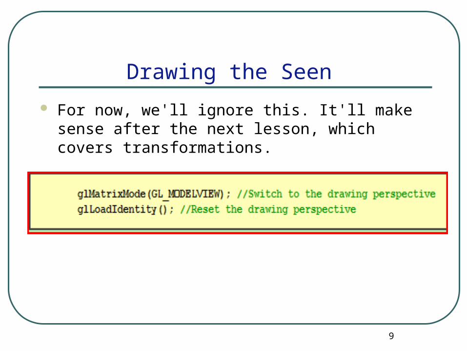
Drawing the Seen
For now, we'll ignore this. It'll make sense after the next lesson, which covers transformations.

10
Drawing Trapezoid
We call glBegin(GL_QUADS) to tell OpenGL that we want to start drawing quadrilaterals.
We specify the four 3D coordinates of the vertices of the trapezoid, in order When we call glVertex3f, we are specifying three (that's where the "3" comes
from) float (that's where the "f" comes from) coordinates

11
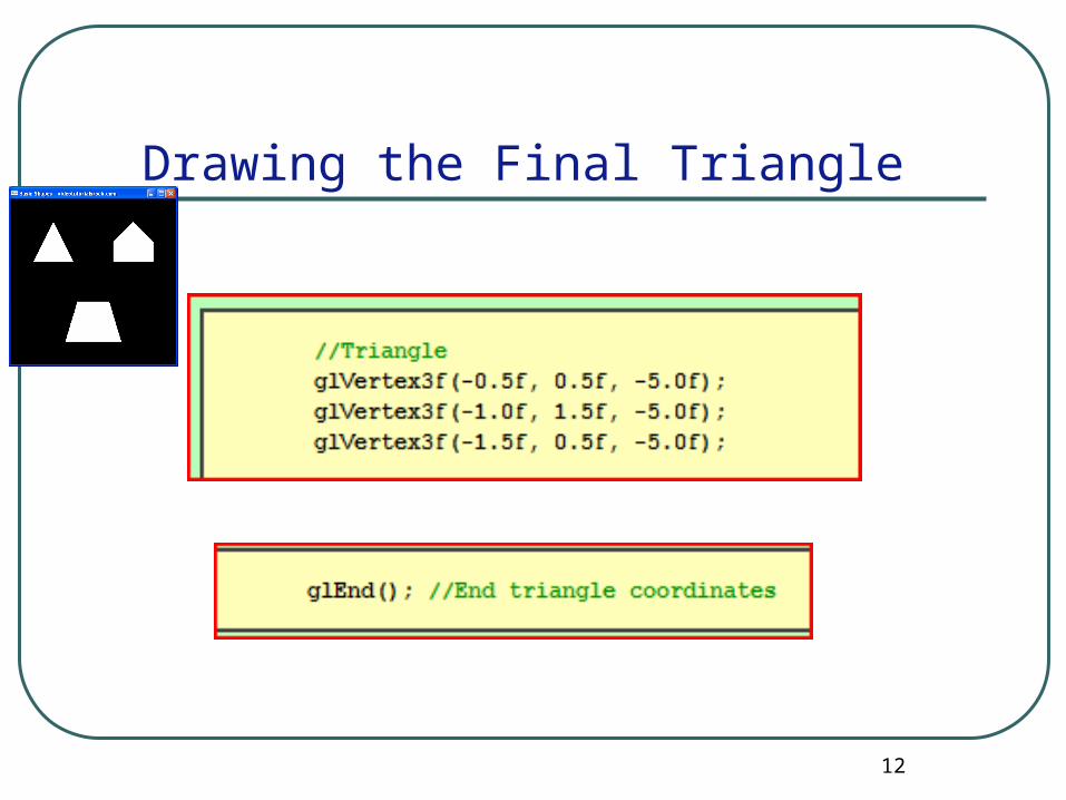
Drawing Pentagon
To draw it, we split it up into three triangles,
12
Drawing the Final Triangle
13
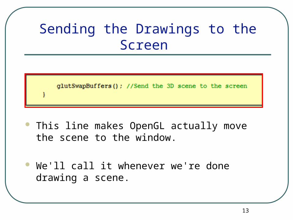
Sending the Drawings to the Screen
This line makes OpenGL actually move the scene to the window.
We'll call it whenever we're done drawing a scene.

14
Calling the main()
In the call to glutInitWindowSize, we set the window to be 400x400. When we call glutCreateWindow, we tell it what title we want for the
window. Then, we call initRendering, the function that we wrote to initialize
OpenGL rendering.

15
handling keypresses and drawing and resizing the window

16
Going in a loop to keep Scene visible

17
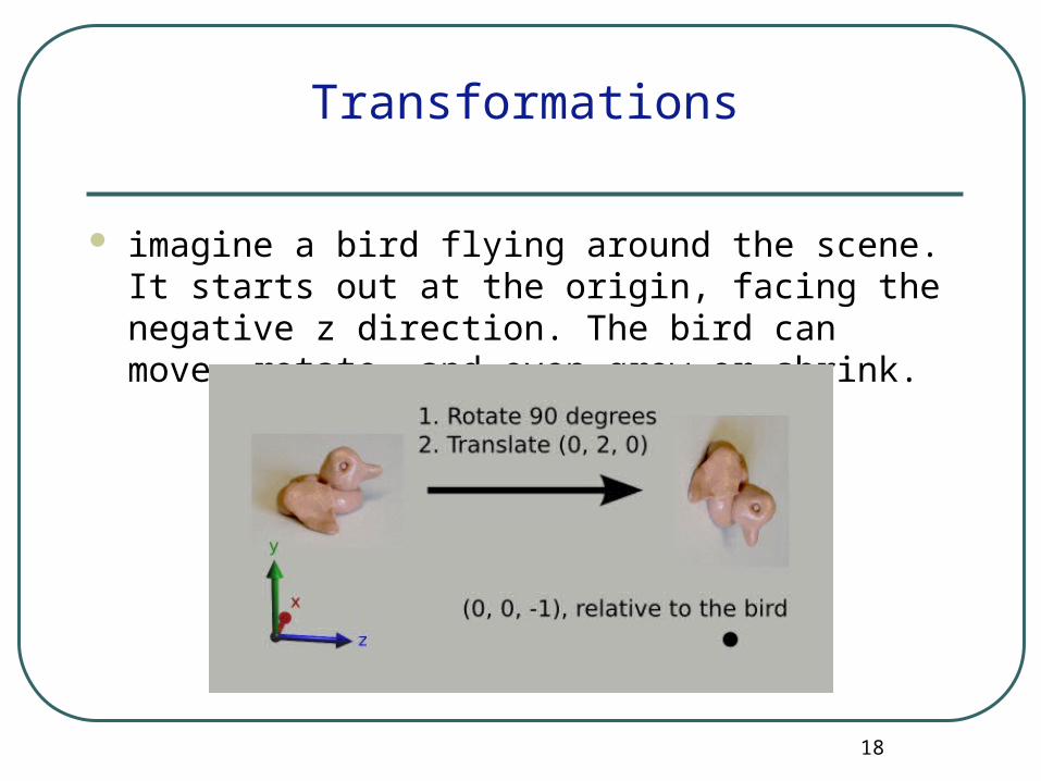
Transformations
We'll make the shapes rotate in 3D.
18
Transformations
imagine a bird flying around the scene. It starts out at the origin, facing the negative z direction. The bird can move, rotate, and even grow or shrink.

Lesson 2 Video
19
Transformations

20
Digital Images and Image Manipulation
Digital image stored as a rectangular array of pixels in the color buffer.
Each pixel value may be a single scalar component, or a vector containing a separate scalar value for each color component.

21
Digital Images and Image Manipulation
Assume that each pixel accurately represents the average color value of the geometric primitives that cover it.
The process of converting a continuous function into a series of discrete values is called sampling.
A geometric primitive, projected into 2D, can be thought of as defining a continuous function of its spatial coordinates x and y.

22
Digital Images and Image Manipulation
For example, a triangle can be represented by a function fcontinuous(x, y).
It returns the color of the triangle when evaluated within the triangle’s extent, then drops to zero if evaluated outside of the triangle.
Note that: • An ideal function has an abrupt change of value at the triangle
boundaries.
• This instantaneous drop-off is what leads to problems when representing geometry as a sampled image.

23
Digital Images and Image Manipulation
The output of the function isn’t limited to a color; it can be any of the primitive attributes: • intensity (color),
• depth, or
• texture coordinates;
To avoid overcomplicating matters, we can limit the discussion to intensity values without losing any generality.

24
Digital Images and Image Manipulation
A straightforward approach to sampling the geometric function is to • Evaluate the function at the center of each pixel in window
coordinates.
The number of samples per unit length in each direction defines the sample rate.
25
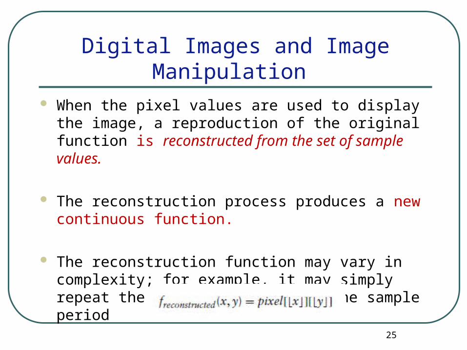
Digital Images and Image Manipulation
When the pixel values are used to display the image, a reproduction of the original function is reconstructed from the set of sample values.
The reconstruction process produces a new continuous function.
The reconstruction function may vary in complexity; for example, it may simply repeat the sample value across the sample period

26
Digital Images and Image Manipulation
Example of image reconstructionExample of image reconstruction
This reconstruction function is complex, involving not only properties of the video circuitry, but also the shape, pattern, and physics of the phosphor on the screen.

27
Digital Images and Image Manipulation
The reliability of the reproduction is a critical aspect of using digital images.
A fundamental concern of sampling • Ensuring that there are enough samples to accurately reproduce the
desired function.
The problem is that a set of discrete sample points cannot capture arbitrarily complicated detail, even if we use the most sophisticated reconstruction function.

28
Digital Images and Image Manipulation
considering an intensity function that has the similar values at two sample points P1 and P3, but between these points P2 the intensity varies significantly
The result is that the reconstructed function doesn’t reproduce the original function very well (Under sampling )

29
Sampling Process To understand sampling, it helps to rely on some
signal processing theory, in particular, Fourier analysis.
In signal processing, the continuous intensity function is called a signal.
This signal is traditionally represented in the spatial domain as a function of spatial coordinates

30
Sampling Process Fourier analysis :
• The signal can be equivalently represented as a weighted sum of sine wavessine waves of different frequencies and phase offsets.
The corresponding frequency domain representation of a signal describes the magnitude and phase offset of each sine wave component.
The frequency domain representation describes the spectral composition of the signal.

31
Sampling Process
From sine wave decomposition, it becomes clear that the number of samples required to reproduce a sine wave must be twice its frequency, assuming ideal reconstruction.
This requirement is called the Nyquist limit.
Generalizing from this result, to accurately reconstruct a signal, the sample rate must be at least twice the rate of the maximum frequency in the original signal.

32
Sampling Process
Reconstructing an undersampled sine wave results in a different sine wave of a lower frequency.
This low-frequency version is called an alias.
Aliased signals in digital images give rise to the familiar artifacts of jaggies, or staircasing at object boundaries.

33
Digital Filtering
Next time ISA.
Related Documents