IMAGE PROCESSING TOOLS FOR QUANTITATIVE ANALYSIS OF ...

The Pennsylvania State University

The Graduate School

Department of Bioengineering

IMAGE PROCESSING TOOLS FOR QUANTITATIVE ANALYSIS OF

MAGNETIC RESONANCE NEUROIMAGING AND APPLICATION TO

AMYOTROPHIC LATERAL SCLEROSIS

A Dissertation in

Bioengineering

by

Don Charles Bigler

© 2009 Don Charles Bigler

Submitted in Partial Fulfillment of the Requirements

for the Degree of

Doctor of Philosophy

May 2009

The dissertation of Don Charles Bigler was reviewed and approved* by the following:

Qing X. Yang Professor of Radiology and Neurosurgery Dissertation Advisor Chair of Committee

Andrew Webb Professor of Bioengineering

Aldo Morales Professor of Electrical Engineering

Craig Meyers Professor of Microbiology and Immunology

Herbert Lipowsky Professor of Bioengineering Head of the Department of Bioengineering

*Signatures are on file in the Graduate School

iii

ABSTRACT

The diagnosis and evaluation of neurodegenerative disease using MRI is qualitative,

subjective, and experience-based. Such conventional approaches are low in information

to data ratio and do not provide quantitative markers for disease evaluation. Currently,

the tools needed for quantitative MRI (qMRI) processing are not adequate for routine

clinical usage. Thus, there is a need for image analysis tools for clinical applications and

trials using qMRI. This work consists of two main parts. a) Software engineering of

image processing tools to enhance and integrate existing advanced registration tools for

processing multi-modality MRI in parallel on a supercomputer and development of an

efficient method to automatically estimate thickness distribution of an anatomical

structure in a medical image. b) Application of the developed tools to a cross-sectional

and longitudinal multi-modality qMRI study of amyotrophic lateral sclerosis (ALS).

The thickness estimation tool was validated using basic shapes with known geometric

dimensions, sample knee and brain MRI. Validation of the tools for their effectiveness

for clinical research applications was performed via a group comparison of mild

cognitive impaired (MCI) subjects with known pathology and normal control subjects.

When applied to ALS cross-sectionally, differences were observed between ALS and

normal controls for cortical thickness, measures of brain volume, T2, and diffusion tensor

imaging (DTI). Longitudinally, the results were mixed. In general, changes due to

disease were subtle, which strongly support the need for an integrated multimodality

approach for detection of neurodegenerative diseases, such as ALS.

iv

TABLE OF CONTENTS

LIST OF FIGURES ..................................................................................................... ix

LIST OF TABLES.......................................................................................................xix

LIST OF ACRONYMS ...............................................................................................xx

ACKNOWLEDGEMENTS.........................................................................................xxv

Chapter 1 Introduction ................................................................................................1

1.1 References.......................................................................................................3

Chapter 2 Quantitative MRI (qMRI) ..........................................................................4

2.1 Introduction.....................................................................................................4 2.2 Transverse relaxation parameter maps ...........................................................5

2.2.1 What is transverse relaxation?..............................................................5 2.2.1.1 Dipole-dipole interaction............................................................10 2.2.1.2 Electron paramagnetism.............................................................10

2.2.2 Acquisition and measurement ..............................................................11 2.2.3 Movement artifact and its correction....................................................17 2.2.4 Significance to neurodegenerative disease ...........................................20

2.3 Diffusion tensor imaging ................................................................................21 2.3.1 What is diffusion tensor imaging?........................................................21 2.3.2 Acquisition and measurement ..............................................................24 2.3.3 Eddy current artifact and its correction ................................................27 2.3.4 Significance to neurodegenerative disease ...........................................32

2.4 Morphological measurements.........................................................................34 2.4.1 Volume .................................................................................................34

2.4.1.1 Brain parenchyma fraction (BPF) ..............................................35 2.4.1.2 Ventricular fraction (VF) ...........................................................36 2.4.1.3 Voxel-based morphometry (VBM) ............................................37

2.4.1.3.1 Regional analysis of volume in normalized space (RAVENS)...............................................................................39

2.4.2 Cortical thickness .................................................................................41 2.4.3 Significance to neurodegenerative disease ...........................................42

2.5 Statistical analysis of images ..........................................................................43 2.5.1 Region of interest (ROI) analysis .........................................................44 2.5.2 Histogram analysis ...............................................................................44 2.5.3 Statistical parametric mapping (SPM)..................................................45

2.5.3.1 Registration ................................................................................45 2.5.3.1.1 Affine linear registration..................................................46 2.5.3.1.2 Non-linear registration .....................................................50

v

2.5.3.2 Smoothing ..................................................................................50 2.5.3.3 General linear model (GLM)......................................................51 2.5.3.4 Statistical inferences and theory of Gaussian random fields......53

2.5.3.4.1 Anatomically closed hypotheses ......................................53 2.5.3.4.2 Anatomically open hypotheses ........................................53

2.6 References.......................................................................................................57

Chapter 3 Software Tool for Automated MRI Post-processing on a Supercomputer (STAMPS)...................................................................................62

3.1 Introduction.....................................................................................................62 3.2 Convert labeled atlas to tissue segmented atlas..............................................65 3.3 Image padding and cropping ..........................................................................66 3.4 Intensity normalization ...................................................................................67 3.5 RAVENS normalization .................................................................................68 3.6 Apply HAMMER deformation field to any data type ....................................72 3.7 Labeled ROI statistics.....................................................................................75 3.8 References.......................................................................................................76

Chapter 4 An Efficient Voxel-based Method for Automatic Estimation of Thickness in Medical Images ...............................................................................78

4.1 Abstract...........................................................................................................78 4.2 Introduction.....................................................................................................79 4.3 Proposed Method ............................................................................................83

4.3.1 Preprocessing........................................................................................85 4.3.2 Lookup table.........................................................................................85 4.3.3 Search ...................................................................................................86

4.3.3.1 Special cases...............................................................................89 4.3.4 Cleanup.................................................................................................90

4.4 Validation .......................................................................................................91 4.4.1 Solid three-dimensional ellipsoid .........................................................91 4.4.2 Three-dimensional ellipsoidal shell......................................................92

4.5 Results.............................................................................................................93 4.5.1 MRI human knee patellar cartilage thickness ......................................94 4.5.2 MRI human brain cortical thickness.....................................................95 4.5.3 MRI SPM paired t-test of MCI and normal controls............................98

4.6 Discussion.......................................................................................................100 4.7 References.......................................................................................................104

Chapter 5 Amyotrophic Lateral Sclerosis (ALS): An Introduction............................108

5.1 Brief history ....................................................................................................108 5.2 Pathology ........................................................................................................108 5.3 Etiology...........................................................................................................109 5.4 Diagnosis ........................................................................................................110

vi

5.5 Neuroimaging .................................................................................................112 5.5.1 PET/SPECT..........................................................................................112 5.5.2 Conventional MRI ................................................................................113 5.5.3 MRS......................................................................................................114 5.5.4 DTI .......................................................................................................115 5.5.5 VBM .....................................................................................................116 5.5.6 fMRI .....................................................................................................116

5.6 References.......................................................................................................117

Chapter 6 ALS Brain Cortical Thickness Analysis ....................................................125

6.1 Abstract...........................................................................................................125 6.2 Introduction.....................................................................................................127 6.3 Materials and methods....................................................................................128

6.3.1 Subjects.................................................................................................128 6.3.2 MR-Imaging protocol ...........................................................................131 6.3.3 Image post-processing ..........................................................................131 6.3.4 Cross-sectional and longitudinal cortical thickness analysis................132 6.3.5 Cross-sectional and longitudinal primary motor thickness analysis ....133 6.3.6 Regional average cortical thickness and cognitive exams ...................134

6.4 Results.............................................................................................................134 6.4.1 Cross-sectional and longitudinal cortical thickness analysis................134 6.4.2 Cross-sectional and longitudinal primary motor cortex thickness

analysis ...................................................................................................135 6.4.3 Regional average cortical thickness and cognitive exams ...................144


Chapter 7 ALS Brain Volumetric Analysis ................................................................148


7.3.1 Subjects.................................................................................................151 7.3.2 MR-Imaging protocol ...........................................................................151 7.3.3 Image post-processing ..........................................................................151 7.3.4 Cross-sectional and longitudinal BPF and VF analysis .......................152 7.3.5 Cross-sectional and longitudinal whole-brain VBM analysis ..............152

7.4 Results.............................................................................................................154 7.4.1 Cross-sectional and longitudinal BPF and VF analysis .......................154 7.4.2 Cross-sectional and longitudinal whole-brain VBM analysis ..............159


Chapter 8 ALS Brain T and DTI Analysis................................................................175 2

vii


8.3.1 Subjects.................................................................................................178 8.3.2 MR-Imaging protocol ...........................................................................179 8.3.3 T relaxometry processing....................................................................180 28.3.4 DTI processing .....................................................................................180 8.3.5 Image registration.................................................................................181 8.3.6 Cross-sectional and longitudinal whole-brain voxel-based analysis....181

8.4 Results.............................................................................................................183 8.4.1 Cross-sectional whole-brain voxel-based analysis ...............................183 8.4.2 Longitudinal whole-brain voxel-based analysis ...................................186


Chapter 9 Summary ....................................................................................................199

9.1 References.......................................................................................................201

Chapter 10 Future Work .............................................................................................203

10.1 Software Tool for Automated MRI Post-processing on a Supercomputer (STAMPS).....................................................................................................203 10.1.1 Brain registration and segmentation...................................................203 10.1.2 Brain atlases........................................................................................204 10.1.3 Hybrid anatomical open hypotheses using ROI statistics ..................208 10.1.4 Preparation for distribution.................................................................208

10.2 An Efficient Voxel-based Method for Automatic Estimation of Thickness in Medical Images ........................................................................209 10.2.1 Touching gyri .....................................................................................209

10.3 ALS...............................................................................................................211 10.3.1 Determine normative longitudinal qMRI variability..........................211 10.3.2 Determine diagnostic value of qMRI .................................................212 10.3.3 Determine pathological causes to qMRI changes ..............................213

10.4 References.....................................................................................................214

Appendix A MR Parameter Map Suite: ITK Classes for Calculating Magnetic Resonance T and T Parameter Maps.................................................................215 2 1

A.1 Abstract..........................................................................................................215 A.2 Background....................................................................................................216

A.2.1 Measuring T relaxation......................................................................217 2A.2.2 Measuring T relaxation......................................................................218 1

A.3 Implementation ..............................................................................................219 A.3.1 itk::MRT2ParameterMap3DImageFilter .............................................220 A.3.2 itk::MRT1ParameterMap3DImageFilter .............................................222

viii

A.3.3 itk::Bruker2DSEQImageIO .................................................................226 A.3.4 itk::PhilipsRECImageIO......................................................................228

A.4 Examples........................................................................................................231 A.4.1 Bruker 2DSEQ T parameter map.......................................................232 2A.4.2 Bruker 2DSEQ T parameter map.......................................................239 1A.4.3 Philips REC T parameter map ...........................................................246 2A.4.4 Philips REC T parameter map ...........................................................254 1

A.5 Conclusion .....................................................................................................261 A.6 References......................................................................................................262

Appendix B Slice Interleaved Movement Artifact Correction C++ Source Code .....264

B.1 PhilipsT2Map.h..............................................................................................264 B.2 PhilipsT2Map.cpp ..........................................................................................267

Appendix C Process Philips DTI tcl and C++ Source Code.......................................298

C.1 call_sourcePhilipsDTIFit.sh...........................................................................298 C.2 sourcePhilipsDTIFit.tcl ..................................................................................298 C.3 PhilipsDTIFit.tcl ............................................................................................299 C.4 philipsparinfo.cxx ..........................................................................................316

Appendix D HAMMER Extensions C++ Source Code..............................................326

D.1 ConvertLabeledAtlasToTissueSegmented.cxx..............................................326 D.2 LinuximagePad.cxx .......................................................................................333 D.3 LinuximageCrop.cxx .....................................................................................338 D.4 vtkImageStatistics.h.......................................................................................342 D.5 vtkImageStatistics.cxx ...................................................................................345 D.6 LinuximageNormalizeIntensity.cxx ..............................................................351 D.7 LinuximageNormalizeRAVENS.cxx ............................................................355 D.8 itkVectorReorderComponentsImageFilter.h..................................................363 D.9 LinuxPerformDeformationOnImgUsingVectorFieldExtended.cxx ..............366 D.10 vtkImageComparison.h................................................................................374 D.11 vtkImageComparison.cxx ............................................................................377 D.12 LinuximageInfoExtended.cxx......................................................................385

Appendix E Automatic Voxel-based Thickness Estimation C++ Source Code.........394

E.1 vtkImageOptimizedThicknessFilter2D.h .......................................................394 E.2 vtkImageOptimizedThicknessFilter2D.cxx ...................................................396 E.3 vtkImageOptimizedThicknessFilter3D.h .......................................................413 E.4 vtkImageOptimizedThicknessFilter3D.cxx ...................................................415

ix

LIST OF FIGURES

Figure 2-1: Vectoral representation of the magnetic moments of three protons aligned parallel with a static magnetic field B . The vector addition of the magnetic moments of the three protons, called magnetization, is labeled M (not to scale). The vectors are shown in the rotating reference frame that rotates at the Larmor frequency ω. .......................................................................7

0

0

Figure 2-2: The magnetization, M , is rotated 90° into the XY plane using an externally applied B field that is perpendicular to B . The direction of rotation follows a left-hand rule (opposite the usual right-hand rule). .................8

0

1 0

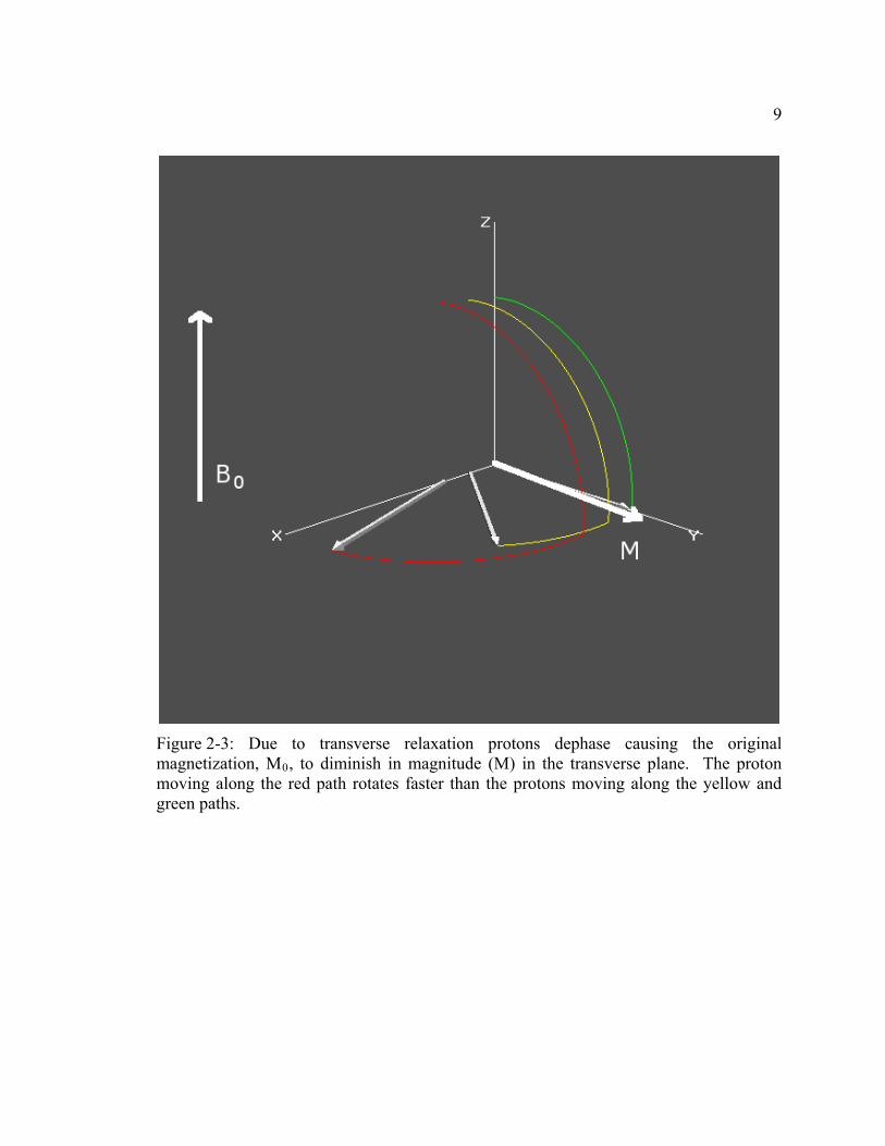
Figure 2-3: Due to transverse relaxation protons dephase causing the original magnetization, M , to diminish in magnitude (M) in the transverse plane. The proton moving along the red path rotates faster than the protons moving along the yellow and green paths..........................................................................9

0

Figure 2-4: After the 90° RF pulse transverse relaxation causes the MR signal to decay. ....................................................................................................................11

Figure 2-5: Application of a 180º RF pulse long the X axis causes the protons to rotate about the X axis. .........................................................................................12

Figure 2-6: After application of the 180º RF pulse the protons continue to rotate in the same direction. The proton following the red path moves faster than the yellow and green protons and catches up to them to maximize the remaining transverse magnetization again, forming a “spin-echo” as seen in Figure 2-7.....13

Figure 2-7: MR signal demonstrating the formation of a “spin-echo” after refocusing of the dephased protons using a 180º RF pulse. The echo forms at a time, TE, after the original 90º pulse. ................................................................14

Figure 2-8: Demonstration of multiple spin-echoes after repeated 180º RF pulses. The peak signal in each spin-echo decreases at a rate determined by the T time of the sample.................................................................................................15

2

Figure 2-10: Slice interleaved movement artifact. The artifact is best seen in the central fissure circled in red..................................................................................17

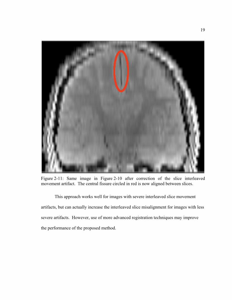
Figure 2-11: Same image in Figure 2-10 after correction of the slice interleaved movement artifact. The central fissure circled in red is now aligned between slices. ....................................................................................................................19

Figure 2-12: The Stejskal-Tanner pulsed field gradient (PFG) spin-echo sequence. The PFG, g, is applied before and after the 180° RF pulse. The interpulse

x

delay, Δ, and the duration of the pulse, δ, define the diffusion time as t = Δ - δ/3 [21]..................................................................................................................22

d

Figure 2-13: Graphical representation of diffusion tensor ellipsoid with eigenvalues ( λ3) and eigenvectors (v ) [22]. .....................................23 1,v2,v3λ1,λ2,

Figure 2-14: A typical single-shot spin-echo EPI sequence used for DTI. G is the diffusion gradient in an arbitrary direction [23]. ............................................25

d

Figure 2-15: Left: Coronal view of FA image. Note the bright signal intensities due to high diffusion anisotropy in the white matter (WM). These areas of high FA highlight the WM fibers. Right: Coronal view of MD for the same subject. MD is high in areas where the water is relatively unrestricted, like in the ventricles and surrounding cerebrospinal fluid (CSF) and is lower in the WM where the diffusion of water is more restricted. ...........................................27

Figure 2-16: Sagittal view of EPI brain image with (a) severe N/2 ghost and (b) little N/2 ghosting [26]..........................................................................................28

Figure 2-17: (a) Arrows point to artificial structures in the brain due to fat chemical shift in EPI. The low bandwidth in the phase encoding or vertical direction causes the shift. (b) The artifact is removed using fat suppression [27]........................................................................................................................29

Figure 2-18: (a) Distortion of the eyes in EPI due to inplane magnetic field inhomogeneities within the eye sockets and nasal cavity. (b) Gradient echo image at the same TE as the EPI image [27]. .......................................................30

Figure 2-19: Demonstration of EPI signal loss in ear canals and sinuses due to through-plane magnetic field inhomogeneities. ...................................................30

Figure 2-20: Examples images of DTI WM fiber tracking..........................................33

Figure 2-21: Left: Coronal view of T -weighted image. Right: Same coronal view of image on left, but with overlay image segmented into gray matter (GM), white matter (WM), and cerebrospinal fluid (CSF). GM is red, WM is yellow, and CSF is light blue................................................................................36

1

Figure 2-22: Coronal view of segmented image in Figure 2-21 with the ventricles relabeled. GM is red, WM is yellow, CSF is light blue, and ventricles are dark blue. ..............................................................................................................37

Figure 2-23: Diagram showing the relationship between voxel-based morphometry (VBM), tensor-based morphometry, and deformation-based morphometry [7]. ..................................................................................................39

xi

Figure 2-24: Orthogonal views of RAVENS image. Higher voxel densities correspond to areas of increased density after warping to an atlas and vice-versa [42]. .............................................................................................................40

Figure 2-25: Sagittal views of gray/white (left), pial (center), and inflated (right) surface representations with overlaid cortical thickness measurements [43]. ......41

Figure 2-26: Manual measurements of thickness for a patient with primary lateral sclerosis in A and B. Similar thickness in C and D for an age and gender matched control subject. B and D show inflated views of the thickness measurements along the anterior (white arrows) and posterior (black arrows) banks of the primary motor cortex and S1 (black arrowheads) [44]. ...................42

Figure 2-27: Application of rotation transform about the origin to a 2-D slice of the brain [53].........................................................................................................47

Figure 2-28: Application of x translation (left) and y translation (right) for a 2-D slice of the brain [53]. ...........................................................................................47

Figure 2-29: Application of a scale > 1 transform in the y direction for a 2-D slice of the brain [53]. ...................................................................................................48

Figure 2-30: Application of a skew transform parallel to the x axis for a 2-D slice of the brain [53]. ...................................................................................................49

Figure 2-31: The general linear model (GLM). In fMRI the data can be filtered with a convolution or residual forming matrix (or a combination) S, leading to a generalized linear model that includes (intrinsic) serial correlations and applied (extrinsic) filtering. S is always 1 for group analysis using qMRI The parameter estimates are obtained in a least squares sense using the pseudoinverse (denoted by +) (see Eq. 2.12) of the filtered design matrix. Generally an effect of interest is specified by a vector of contrast weights c that give a weighted sum or compound of parameter estimatesβ ̂referred to as a contrast. The T statistic is simply this contrast divided by its estimated standard error (i.e. square root of its estimated variance). The ensuing T statistic is distributed with ν v degrees of freedom. The equations for estimating the variance of the contrast and the degrees of freedom associated with the error variance are provided in the right-hand panel. Efficiency is simply the inverse of the variance of the contrast. These expressions are useful when assessing the relative efficiency of experimental designs. The parameter estimates can either be examined directly or used to compute the fitted responses (see lower left panel). Adjusted data refers to data from which estimated confounds have been removed. The residuals r is obtained from applying the residual-forming matrix R to the data. These residual fields are used to estimate the smoothness of the component fields of the SPM used in random field theory (see Figure) [7]. ..............................................52

xii

Figure 2-32: Schematic illustrating the use of Random Field theory in making inferences about SPM's. This schematic deals with a general case of n SPM{T} whose voxels all survive a common threshold u (i.e. a conjunction of n component SPM’s). The central probability, upon which all voxel, cluster or set-level inferences are made, is the probability P of getting c or more clusters with k or more resels (resolution elements) above this threshold. By assuming that clusters behave like a multidimensional Poisson point process (i.e. the Poisson clumping heuristic) P is simply determined. The distribution of c is Poisson with an expectation that corresponds to the product of the expected number of clusters, of any size, and the probability that any cluster will be bigger than k resels. The latter probability is shown using a form for a single Z-variate field constrained by the expected number of resels per cluster (<.> denotes expectation or average). The expected number of resels per cluster is simply the expected number of resels in total divided by the expected number of clusters. The expected number of clusters is estimated with the Euler characteristic (EC) (effectively the number of blobs minus the number of holes). This estimate is in turn a function of the EC density for the statistic in question (with ν degrees of freedom v) and the resel counts. The EC density is the expected EC per unit of D-dimensional volume of the SPM where the D dimensional volume of the search space is given by the corresponding element in the vector of resel counts. Resel counts can be thought of as a volume metric that has been normalized by the smoothness of the SPM’s component fields expressed in terms of the full width at half maximum (FWHM). This is estimated from the determinant of the variance-covariance matrix of the first spatial derivatives of e, the normalized residual fields r (from Figure 2-31). In this example equations for a sphere of radius θ are given. Φ denotes the cumulative density function for the sub-scripted statistic in question [7]. ..............................................................55

Figure 2-33: Graphical depiction of the subset of SPM above threshold (connected excursions) [54]..................................................................................56

Figure 3-1: Post-processing in STAMPS for T -weighted images [1]........................63 1

Figure 3-3: Whole-brain SPM of 33 RAVENS white matter (WM) images. A multiple regression model using whole-brain volume and age as covariates was used. The statistics maps were obtained using a false discovery rate (FDR) of 0.05 and 0 voxel extent. ........................................................................69

Figure 3-4: Whole-brain SPM of 33 normalized RAVENS white matter (WM) images. A multiple regression model using whole-brain volume and age as covariates was used. The statistics maps were obtained using a false discovery rate (FDR) of 0.05 and 0 voxel extent..................................................71

xiii

Figure 3-5: Axial view of a HAMMER deformation field midway through the volume. The color is mapped to the magnitude of the vector at each voxel location. 3D arrow glyphs demonstrate the magnitude and direction of deformation. The faint outline of the brain may be seen in the center of the slice. ......................................................................................................................73

Figure 3-6: Axial view of a corrected HAMMER deformation field midway through the volume. The color is mapped to the magnitude of the vector at each voxel location. 3D arrow glyphs demonstrate the magnitude and direction of deformation. The vector components of the deformation were reordered from Y, X, Z format to X, Y, Z format for use in ITK.........................74

Figure 4-1: Flowchart outlining the iterative search algorithm used to calculate thickness using the EDT. ......................................................................................84

Figure 4-2: Example binary object (a) and the same binary object after application after application of the EDT. The values shown in (b) are the squared Euclidean distances to the nearest zero pixel. ......................................................85

Figure 4-3: Graphical representation of lookup table list structure for the squared Euclidean distance map shown in Figure 4-2(b). Each list element references a squared Euclidean distance value and a list of coordinates indicating the locations of the squared Euclidean distance value within the 2-D image. ...........86

Figure 4-4: Graphical depiction of the search algorithm for a pixel thickness of four. The circular outline in (a) depicts the search area for the squared Euclidean distance of five. Lines that pass through the center of the circle and are bordered by zeros just outside the circle are labeled with four in (b). .....88

Figure 4-5: Following the search for four pixel thicknesses in Figure 4-4, the search continues with three pixel thicknesses in (a). Only those pixels that were not marked previously are marked in (b)....................................................................88

Figure 4-6: Graphical depiction of special cases handled explicitly in the proposed method. (a) demonstrates the two pixel case. Adjacent ones bordered by zeros in orthogonal directions are marked with two in (b) for the binary object example. Two pixel thicknesses are a special case of the more general even and odd problem associated with discrete data shown for four pixels in (c). The EDM in (c) does not have a center pixel for the search circle. ..............89

Figure 4-7: Graphical depiction of special single pixel cases handled explicitly in the proposed method. The zeros are shown in (a) to demonstrate how the proposed method searches each direction for a one surrounded by zeros in any of the directions shown. The final thickness distribution map (TDM) for the binary object example is shown in (b). ...........................................................90

xiv

Figure 4-8: Grayscale maps of Euclidean distance (a) and thickness distribution (b) for a 3-D ellipsoid with pixel radii of 64, 32, and 8 for the x, y, and z-axes respectively. The top views in each figure show the entire ellipsoids and the bottom views show cross-sectional views of the ellipsoids midway through the x-axis. The maximum thickness measured is 16, which is twice the z radius or the smallest radius specified for the ellipsoid........................................92

Figure 4-9: Grayscale maps of Euclidean distance (a) and thickness distribution (b) for a 3-D ellipsoid shell. The outer ellipsoid has pixel radii of 64, 32, and 16 for the x, y, and z-axes respectively. The inner ellipsoid has pixel radii of 58, 28, and 8 for the x, y, and z-axes respectively. The top views in each figure show the entire ellipsoids and the bottom views show cross-sectional views of the ellipsoids midway through the x axis. As expected the maximum thickness measured is 8 (difference between z radii) and the minimum thickness is 4 (difference between y radii)...........................................93

Figure 4-10: Human patellar cartilage TDM calculated from MR image. The left image displays the sagittal view of the MR T -weighted water selective fluid scan of human knee (0.313 mm isotropic voxel size) with an overlay of the patellar cartilage TDM. The images on the right are 3-D volume renderings of the TDM and image mask for the patellar cartilage. A section of the cartilage was removed to display the inner thickness distribution. Average thickness was 3.011 mm. ......................................................................................95

1

Figure 4-11: Brain cortical TDM derived from the automatically-segmented image set. Three orthogonal projections of T -weighted MR image of human head (left), the cortical TDM overlay (middle), and 3-D volume renderings of the TDM and image mask (right) are shown. The average cortical thickness was 3.14 mm.........................................................................................................97

1

Figure 4-12: SPM t-maps for paired t-test of NC > MCI overlaid on the average smoothed cortical TDM of all of the subjects. A false discovery rate (FDR) of 0.05 and voxel extent of 100 was used to threshold the t-maps. (a) Right hippocampal formation. (b) Bilateral cingulate region. (c) Left hippocampal formation. (d) Bilateral thalamus.........................................................................100

Figure 4-13: Thickness map of Figure 4-6(c) that illustrates problem where abrupt change in object boundary causes the algorithm to miss corner pixels. Increasing the size of the search circle so that it encloses the object will cause the corner pixels to also be marked with four.......................................................102

Figure 4-14: Illustration showing the ambiguities that exist in the EDM for low resolution digital circles. Digital circles with radii 1 and 1.5 are exactly the same. The EDM for digital circles with radii 2 and 2.5 both have five at their centers, even though their shapes are different. The proposed method

xv

described in Section 4.3 will favor thicker values over thinner values in the case of ambiguities. ..............................................................................................104

Figure 5-1: Revised El Escorial clinical diagnostic groups [14]. ................................112

Figure 6-1: Scatter plot of right primary motor cortex (PMC) thickness versus age for the ANCOVA model grouped by Controls = C, ALS Limb only = L, and ALS Generalized (Limb and Bulbar) = G (defined in Table 6-1). The ALS Limb group was significant (P = 0.0322). The ALS Generalized approached significance (P = 0.0792). The correlation of thickness with age for each group is also plotted..............................................................................................136

Figure 6-2: Scatter plot of right primary motor cortex (PMC) thickness versus age for the ANCOVA model grouped by Controls = C and El Escorial classification. Table 6-1 defines the El Escorial symbols used in the plot. The ALS Probable group was significant (P = 0.0006) and the ALS Definite group approached significance (P = 0.0893). The correlation of thickness with age for the Control, ALS Probable, and ALS Definite groups are also plotted. ..................................................................................................................137

Figure 6-3: Scatter plot of right postcentral gyrus (PCG) thickness versus age for the ANCOVA model grouped by Controls = C and El Escorial classification. Table 6-1 defines the El Escorial symbols used in the plot. The ALS Probable group was significant (P = 0.0027). The correlation of thickness with age was not significant. ................................................................................138

Figure 6-4: Scatter plot of ALS left primary motor cortex (PMC) age corrected thickness versus time in months from baseline scan. The significant (P = 0.0185) regression line is also plotted. The subjects are listed in Table 6-1. ......140

Figure 6-5: Scatter plot of ALS left primary motor cortex (PMC) age corrected thickness versus disease duration from onset of symptoms in months. The significant (P = 0.0093) regression line is also plotted. The subjects are listed in Table 6-1...........................................................................................................141

Figure 6-6: Scatter plot of ALS left primary motor cortex (PMC) age corrected thickness versus the Revised ALS Functional Rating Score (ALSFRS-R). The significant (P = 0.0007) regression line is also plotted. The subjects are listed in Table 6-1. ................................................................................................142

Figure 6-7: Scatter plot of ALS left postcentral gyrus (PCG) thickness versus disease duration from onset of symptoms in months. The significant (P = 0.0134) regression line is also plotted. The subjects are listed in Table 6-1. ......143

Figure 7-1: Scatter plot of age corrected brain parenchyma fraction (BPF) (expressed as a percent) versus disease duration in months from onset of

xvi

symptoms for ALS subjects grouped by limb only and generalized (limb and bulbar). The correlation of BPF with duration was significant (P = 0.0425) for the generalized group. The subjects are listed in Table 6-1...........................155

Figure 7-2: Scatter plot of ALS ventricular fraction (VF) (expressed as a percent) versus time in months from baseline scan. VF correlated significantly (P = 0.0576) with time; the regression line is plotted. The subjects are listed in Table 6-1...............................................................................................................157

Figure 7-3: Scatter plot of ALS ventricular fraction (VF) (expressed as a percent) versus disease duration in months from onset of symptoms. VF correlated significantly (P = 0.0528) with duration; the regression line is also plotted. The subjects are listed in Table 6-1. .....................................................................158

Figure 7-4: Orthogonal views of RAVENS GM for brain regions listed in Table 7-1: (a) right precentral gyrus overlapping onto right postcentral gyrus, (b) left postcentral gyrus, (c) left superior parietal lobule, (d) right superior parietal lobule, (e) right middle temporal gyrus, (f) right middle temporal gyrus, (g) left middle temporal gyrus, (h) right lateral fronto-orbital gyrus overlapping onto left lateral fronto-orbital gyrus, and (i) left lateral fronto-orbital gyrus. The t-values (0.001 uncorrected p-value and 50 voxel extent) are overlaid on the smoothed average RAVEN GM image for all subjects. ........160

Figure 7-5: Orthogonal views of RAVENS WM for brain regions listed in Table 7-1: (a) left parietal lobe WM near left postcentral gyrus and superior parietal lobule, (b) left parietal lobe WM near left superior parietal lobule, (c) left parietal lobe WM near left angular and supramarginal gyri, (d) right temporal lobe WM near right middle temporal gyrus, (e) right parietal lobe WM near right postcentral gyrus, (f) right parietal lobe WM near right postcentral gyrus, (g) left frontal lobe WM near left medial frontal and precentral gyri, and (h) left frontal lobe WM near left precentral gyrus. The t-values (0.001 uncorrected p-value and 50 voxel extent) are overlaid on the smoothed average RAVEN WM image for all subjects. ......................................161

Figure 7-6: 3D views of longitudinal (a) RAVENS GM and (b) RAVENS WM results. Red clusters show significant (0.05 false discovery rate and 50 voxel extent) decrease in volume using the paired t-test between baseline and 6 month ALS subjects, green clusters show significant negative correlation of volume with disease duration from onset of symptoms, and blue clusters show significant negative correlation of volume with time from baseline...........164

Figure 8-1: Radiological coronal, sagittal, and axial views of clusters of significant (0.001 uncorrected p-value and 100 voxel extent) ALS and control group differences for T relaxometry (red), DTI FA (blue), and DTI MD (green) overlaid on the average smoothed DTI FA image of all the subjects. (a) Clusters of significantly increased T are shown in the 1) left subcortical

2

2

xvii

superior/medial frontal gyrus and within the 2) left medial frontal gyrus (MeFG). Significant decreases in DTI FA are also shown in the 3) left cerebellum, 4) left subcortical PMC, and 5) right PCG. (b) Clusters of significantly decreased DTI FA in the 6) bilateral CST at the cerebral peduncles (CP), the 7) right subcortical PMC, and the 8) right cerebellum are shown. Clusters of significantly increased DTI MD occurred in the 9) right CST at the CP and 10) corona radiata (CR) and in the 11) left insula. The Axial view shows an increase of T in the 12) right superior temporal gyrus (STG). (c) Clusters of significantly decreased DTI FA in the 13) bilateral subcortical PMC, in the 14) right PG, and in the 15) right cerebellum are shown. Also shown is the increase of MD in the 9) CST at the CP and in the 16) right PCG (overlapping with DTI FA). (S = Superior, I = Inferior, R = Right, L = Left, A = Anterior, and P = Posterior) ................................................184

2

Figure 8-2: Radiological coronal, sagittal, and axial views of clusters of significant (0.05 false discovery rate and 100 voxel extent) longitudinal positive correlation of ALS T relaxometry (red) and DTI MD (green) with disease duration from onset of symptoms. As seen in the figure, a considerable amount of spatial overlap exists between positive disease correlated DTI MD and positive disease correlated T . The largest clusters occur in the bilateral frontal lobe WM (FLWM), bilateral inferior frontal gyrus (IFG), bilateral cingulate region, and the left superior temporal gyrus (STG). ...................................................................................................................188

2

2

Figure 8-3: Radiological coronal, sagittal, and axial views of clusters of significant (0.05 false discovery rate and 100 voxel extent) longitudinal positive correlation of ALS DTI FA with disease duration from onset of symptoms. The largest clusters occur in the bilateral superior corona radiata (CR) of the corticospinal tract (CST), with smaller clusters in the frontal lobe WM (FLWM) and the left middle frontal gyrus (MiFG). ....................................189

Figure 8-4: Figure 8-2 side-by-side longitudinal RAVENS GM results from Chapter 7, Section 7.4.2. All three image types (T , DTI MD, and RAVENS GM) demonstrate GM atrophy associated with disease duration in overlapping regions. .............................................................................................192

2

Figure 10-1: Coronal views of average registered GM, WM, and CSF probability images and final labeled atlas for 46 subjects between 37 and 81 years of age [3]..........................................................................................................................206

Figure 10-2: Diagram of touching brain gyri...............................................................210

Figure 10-3: Brain gyri after segmentation..................................................................210

Figure A-1: Output from Bruker T parameter map example. The image on the left is the T parameter map, the middle image is the constant S , and the

2

2 0

xviii

right image is the R-squared map. The tube numbers from Table A-1 are labeled in red on the T parameter map image. Note that some contrast exists amongst the tubes in the constant image S . This indicates that the TR of 1595.03 ms was not long enough to remove the contributions due to T in Eq. A.1. .................................................................................................................238

2

0

1

Figure A-2: A plot of image intensity (S ) as a function of TE for a pixel in the center of tube 1 with overlay of fitted curve. Visually, the fitted curve matches the experimental data very well..............................................................239

i

Figure A-3: Output from Bruker T parameter map example. The image on the top left is the T parameter map, the top middle image is the constant S , the top right image is the constant B, and the bottom middle image is the R-squared map. The tube numbers from Table A-1 are labeled red on the T parameter map image. Unlike Figure A-1 very little contrast exists in the constant image S . This indicates that the TE of 10 ms was short enough to remove the contributions due to T in Eq. A.1.....................................................244

1

1 0

1

0

2

Figure A-4: A plot of image intensity (Si) as a function of TR for a pixel in the center of tube 1 with overlay of fitted curve. Again, this demonstrates that the predicted data is a good fit for the experimental data.....................................246

Figure A-5: Output from Philips T parameter map example. The image on the left is the T parameter map, the middle image is the constant S , and the right image is the R-squared map. Like Figure A-1 significant T contrast exists in the constant image S due to the extremely short TR of 252.901 ms. ...253

2

2 0

1

0

Figure A-6: A plot of MR image intensity (S ) as a function of TE for a pixel in the center of the gray matter sphere used in the Philips T parameter map example with overlay of fitted curve. The exponential image intensity points are noisy due to the short TR 252.901 ms and SENSE factor 2.5. A reasonable fit was obtained in spite of the expected variation in the experimental data points. ......................................................................................254

i

2

Figure A-7: Output from Philips T parameter map example. The image on the left is the T parameter map, the middle image is the constant S , and the right image is the R-squared map. The tube numbers from Table A-2 are labeled in read on the T parameter map image. ..................................................259

1

2 0

1

xix

LIST OF TABLES

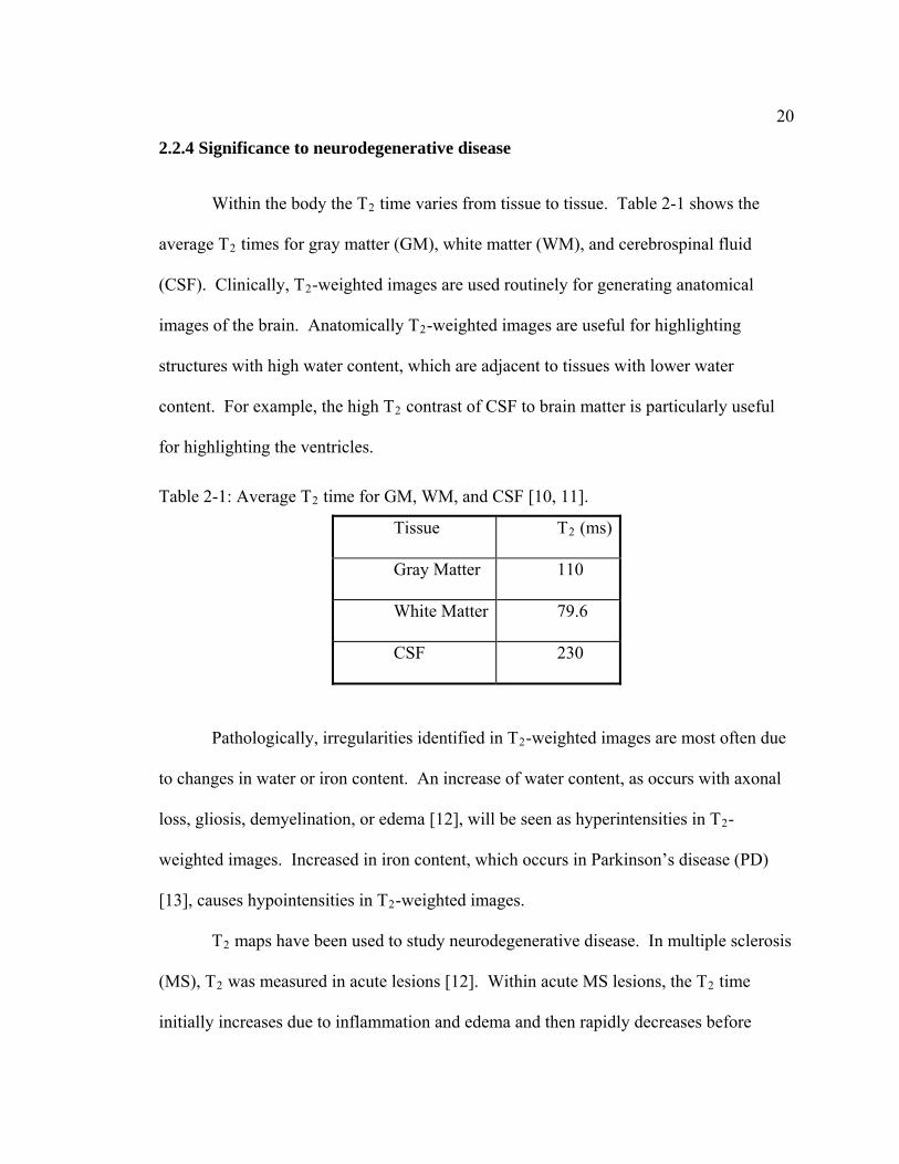
Table 2-1: Average T time for GM, WM, and CSF [10, 11]. ....................................20 2

Table 4-1: Pixel thickness and corresponding squared Euclidean distance mappings...............................................................................................................87

Table 4-2: Voxel thickness and corresponding Euclidean distance mappings. ...........103

Table 6-1: ALS Patient demographic and disease information for baseline, 6 month, 12 month, and 18 month visits. ................................................................130

Table 6-2: Cortical thinning in association with PSSFTS subtest deficiencies in an ALS sample......................................................................................................144

Table 7-1: P-values and average volume loss for cross-sectional regions applied to longitudinal ALS RAVENS GM and WM statistical models. Average volume loss is shown only for regions that are significant or that approached significance (p-value < 0.10). ...............................................................................163

Table 8-1: P-values for cross-sectional T relaxometry, DTI FA, and DTI MD regions examined across modalities. For T relaxometry and DTI MD the p-value is generated from ALS > controls using ANCOVA with age and DTI FA is controls > ALS using ANCOVA with age. ................................................186

2

2

Table 8-2: P-values for cross-sectional regions applied to longitudinal T relaxometry, DTI FA, and DTI MD statistical models. All p-values assume either positive or negative correlation depending on the image type and the covariate. For T relaxometry and DTI MD, paired t-test was 6 months > baseline, time and duration were positive, and ALSFRS-R was negative. DTI FA was the reverse................................................................................................190

2

2

Table A-1: Gd-DTPA and agar concentrations used for Bruker examples. ................231

Table A-2: Gd-DTPA concentrations for phantom used in Philips T example. ........232 1

Table A-3: Average T , S , and R-squared value for each tube in the Bruker T phantom example..................................................................................................238

2 0 2

Table A-4: Average T , S , constant B, and R-squared value for each tube in the Bruker T phantom example. ...............................................................................245

1 0

1

Table A-5: Average T , S , and R-squared value for each tube in the Philips T phantom example..................................................................................................260

1 0 1

xx

LIST OF ACRONYMS

AD Alzheimer’s disease

ADC apparent diffusion coefficient

AG angular gyrus

ALS amyotrophic lateral sclerosis

ALSFRS-R ALS Functional Rating Score-Revised

ANOVA analysis of variance

ANCOVA analysis of covariance

BPF brain parenchyma fraction

CC corpus callosum

CDR Clinical Dementia Rating

CN caudate nucleus

CNMRR Center for Nuclear Magnetic Resonance Research

CNR contrast-to-noise ratio

CNS central nervous system

CP cerebral peduncles

CR corona radiata

CSF cerebrospinal fluid

CST corticospinal tract

CT computed tomography

DTI diffusion tensor imaging

DWI diffusion weighted image

xxi

EPI echo planar image

EMG electromyography

EDM Euclidean distance map

EDT Euclidean distance transform

FA fractional anisotropy

FDR false discovery rate

FL frontal lobe

FLAIR fluid attenuated inversion recovery

FLWM frontal lobe WM

FWHM full width at half maximum

FLTD frontal lobe-type dementia

fMRI functional MRI

FSL FMRIB software library

Gd-DTPA gadolinium-diethylenetriamine penta-acetic acid

GLM general linear model

GM gray matter

GP globus pallidus

GRF Gaussian random fields

GUI graphical user interface

HAMMER hierarchal attribute matching mechanism for elastic registration

H-MRS proton MRS

IFG inferior frontal gyrus

ITG inferior temporal gyrus

xxii

LFOG lateral front-orbital gyrus

LG lingual gyrus

LMN lower motor neuron

MCI mild cognitive impaired

MD mean diffusivity

MeFG medial frontal gyrus

MFOG medial front-orbital gyrus

MiFG middle frontal gyrus

MOTG medial occipitotemporal gyrus

MR magnetic resonance

MRI magnetic resonance imaging

MRS magnetic resonance spectroscopy

MS multiple sclerosis

MTG middle temporal gyrus

NC normal control

OASIS open access series of imaging studies

PD Parkinson's disease

PET positron emission tomography

PFG pulsed field gradient

PCG postcentral gyrus

PL parietal lobe

PLIC posterior limb of internal capsule

PLS primary lateral sclerosis

xxiii

PMA primary muscular atrophy

PMC primary motor cortex

PSC primary sensory cortex

PSSFTS Penn State Screen Exam of Frontal and Temporal Dysfunction Syndromes

qMRI quantitative MRI

RAVENS regional analysis of volume in normalized space

RF radiofrequency

ROI region of interest

SMG supramarginal gyrus

SN septal nuclei

SNR signal-to-noise ratio

SOD1 superoxide dismutase 1

SPECT single photon emission computed tomography

SPM statistical parametric mapping

SPL superior parietal lobule

STAMPS software tool for automated MRI post-processing on a supercomputer

STG superior temporal gyrus

SVM support vector machine

TDM thickness distribution map

TL temporal lobe

UMN upper motor neuron

VB-DTI voxel-based DTI

VBM voxel-based morphometry

xxiv

VBR voxel-based relaxometry

VF ventricular fraction

WM white matter

xxv

ACKNOWLEDGEMENTS

First of all, I would like to thank my wonderful wife Katie for supporting me

through this Ph.D. process. She was my link to sanity and humanity these last six and a

half years and I love her very much.

Second, I’d like to thank Dr. Qing Yang for his unfailing support as a supervisor

and advisor, fellow lab members for their encouragement, and to my committee members

for their valuable input and sacrificed time.

Most importantly I must thank my Heavenly Father for answering numerous

prayers and blessing me with the good health necessary to perform this work.

This thesis is dedicated to my father, Albert Charles Bigler, who taught me to

never give up and always retain hope, even when things are hard or don’t turn out as

expected.

Chapter 1

Introduction

The long-term objective of this research is to develop a set of image analysis tools

and methodology for the detection and quantification of neurodegenerative diseases,

including Alzheimer's disease (AD) and amyotrophic lateral sclerosis (ALS), based on

quantitative processing and analysis of multimodality magnetic resonance imaging (MRI)

data. Currently, the diagnosis and evaluation of neurodegenerative disease using MRI is

qualitative, subjective, and experience-based. Such conventional approaches, although

useful, are low in information to data ratio and do not provide quantitative markers for

disease evaluation. In addition, “the demand from pharmaceutical companies and

neurologists for quantitative MRI (qMRI) measurements to be used in drug trials is large

and likely to increase”[1]. Large drug trials are costly and last for several years. qMRI

methods have the potential to decrease costs and shorten trial lengths by identifying

treatment failures in the early stages of the trial [1]. Currently the tools needed for qMRI

processing are not adequate for routine clinical usage. Thus, there is a need for image

analysis tools for clinical applications and trials using qMRI.

To address this problem, image analysis tools and methodologies were developed

to encompass three specific aims:

1) Develop a more efficient and improved method for processing multimodality

qMRI data that include:

2

Transverse relaxation maps or T2 maps, diffusion tensor imaging (DTI), and

morphological MRI data.

2) Develop an efficient method for estimating thickness in medical images. The

developed image analysis tools were validated for clinical research applications via a

group comparison of mild cognitive impaired (MCI) subjects with known pathology and

normal control subjects.

3) Apply the developed tools to a cross-sectional and longitudinal ALS brain

study. The following hypothesis for the ALS brain study was tested:

I. The abnormalities within the regions identified by qMRI are correlated to the

specific dysfunctions and severity scales of the disease.

Quantitative MRI with focus on DTI, transverse relaxation parameter maps, and

statistical analysis of image data is discussed in Chapter 2. Chapter 3 describes tools

developed for automatic MRI post processing on a super computer (STAMPS) in support

of specific aim 1. In support of specific aim 2, Chapter 4 presents an algorithm for

automatic voxel-based thickness estimation in medical images; which is fast for most

medical images. Chapter 5 presents background information for ALS. This background

will be used for Chapters 6, 7, and 8. These chapters contain methods, results, and

discussions for cortical thickness, volume, T2 maps and DTI respectively. Finally,

Chapter 9 concludes with a summary of the thesis and Chapter 10 discusses future work.

3

1.1 References

[1] P. S. Tofts, "Concepts: Measurement and MR," in Quantitative MRI of the brain: measuring changes caused by disease, P. Tofts, Ed. West Sussex, England: John Wiley & Sons Ltd, 2003, pp. 5-15.

Chapter 2

Quantitative MRI (qMRI)

2.1 Introduction

Quantitative MRI (qMRI) is a field of MRI dedicated to measuring disease

changes in-vivo using MRI. MRI provides a diverse range of qMRI methods, including:

proton density, longitudinal relaxation time (T1), transverse relaxation time (T2),

diffusion tensor imaging (DTI), magnetization transfer, magnetic resonance spectroscopy

(MRS), T1-weighted dynamic contrast-enhanced MRI, blood perfusion and volume

estimation using bolus tracking, functional MRI (fMRI), blood perfusion measurements

using arterial spin labeling, and morphological measurements. This chapter is not meant

to be an exhaustive treatment of qMRI, but provide background information for the qMRI

methods used in the remaining chapters, namely transverse relaxation parameter maps,

DTI, morphological measurements, and the statistical analysis of image data. For a more

detailed treatment of qMRI and the topics covered in this chapter, the reader should refer

to the book by Paul Tofts [1]. In particular Sections 2.2 and 2.3 are covered in more

detail in Chapters 6 and 7 of Tofts’ book. Also, for an excellent introduction to the

mathematics of diffusion tensor imaging, the reader is encouraged to read the three part

journal article series by Peter Kingsley [2-4]. Many of the equations provided in Section

2.3 are covered in more detail in Kingsley’s papers. More advanced mathematical DTI

methods can be found in a recent article by Lenglet and colleagues [5]. Arthur W. Toga’s

5

book [6] on brain warping provides an excellent coverage of the major brain registration

methods. Finally, for a good introduction on statistical parametric mapping (SPM) see

Karl Friston’s chapters in the book Human Brain Function [7] or read his online notes at

http://www.fil.ion.ucl.ac.uk/spm/doc/intro/.

2.2 Transverse relaxation parameter maps

2.2.1 What is transverse relaxation?

Transverse relaxation or spin-spin relaxation is a physical mechanism that causes

exponential signal decay of the transverse component of the MR signal. Transverse in

this case means the plane perpendicular to the direction of the main static magnetic field

B0. In the case of MRI, the MR signal is acquired from the hydrogen or protons within

the patient’s body. Placing a patient within a static magnetic field causes the magnetic

moments of the patient’s protons to align themselves parallel to the direction of the field,

similar to Figure 2-1. Figure 2-1 shows three protons represented by their vector

magnetic moments aligned with a static magnetic field B0 that points in the direction of

the positive Z-axis. The vector sum of all three protons is called the magnetization and is

denoted M0. As shown in Figure 2-1, the vectors are stationary. In actuality the vectors

rotate or precess around the Z-axis at a frequency determined by the Larmor equation

(Eq. 2.1 ):

0B 2.1ω = γ

http://www.fil.ion.ucl.ac.uk/spm/doc/intro/

6

where γ is the gyromagnetic ratio. For protons γ/2π = 42.576 MHz/T. For ease of

demonstration, the vectors in Figure 2-1 and in the remaining figures throughout this

section and the next are shown using a reference frame that rotates at the Larmor

frequency ω. Using this reference frame the vectors will appear stationary about the Z-

axis when they precess at the Larmor frequency.

The MR signal is obtained by perturbing the system with another magnetic field,

B1, which is applied perpendicular to B0. By application of the Lorentz Force Law, M0

will be rotated away from the Z-axis towards the XY plane. The B1 field is generated

using a radiofrequency (RF) coil used for transmission and signal reception. The

maximum MR signal occurs when M0 is rotated exactly 90º such that it lies entirely in

the XY plane as shown in Figure 2-2. The angle of rotation or flip angle is determined by

the duration of the applied B1 field and is given by Eq. 2.2:

tB1γθ = 2.2

where t is time. If transverse relaxation did not exist, the MR signal could be measured

as long as it takes M0 to return to equilibrium, i.e. return so that the proton magnetic

moments point in the direction of the Z-axis again. This longitudinal relaxation time or

T1 is usually much longer than the transverse relaxation time. However, once in the

transverse plane the protons will “dephase” due to transverse relaxation as shown in

Figure 2-3. The net magnetization at this point, denoted by M, will decrease rapidly due

to vector cancellation. Dephasing of the transverse signal occurs because each proton

experiences a slightly different magnetic field. Dephasing due to B0 field

7

inhomogeneities, T2*, is recoverable, whereas dephasing due to spin-spin interactions,

T2, is not. The causes of transverse relaxation will be described in the next subsections.

Figure 2-1: Vectoral representation of the magnetic moments of three protons alignedparallel with a static magnetic field B0. The vector addition of the magnetic moments of the three protons, called magnetization, is labeled M0 (not to scale). The vectors are shown in the rotating reference frame that rotates at the Larmor frequency ω.

8

Figure 2-2: The magnetization, M0, is rotated 90° into the XY plane using an externallyapplied B1 field that is perpendicular to B0. The direction of rotation follows a left-hand rule (opposite the usual right-hand rule).

9

Figure 2-3: Due to transverse relaxation protons dephase causing the original magnetization, M0, to diminish in magnitude (M) in the transverse plane. The protonmoving along the red path rotates faster than the protons moving along the yellow andgreen paths.

10

2.2.1.1 Dipole-dipole interaction

The individual protons within a sample do not stay stationary. As the protons

move about, their magnetic dipole moments interact with each other, perturbing their

local magnetic fields. This dipole-dipole interaction is the most important cause of

transverse relaxation for protons and is related to the internuclear separation of the nuclei.

At short internuclear distances the T2 time is shortened causing faster transverse

relaxation and vice-versa.

2.2.1.2 Electron paramagnetism

The electron magnetic moment is three orders of magnitude greater than protons.

This is important for paramagnetic atoms with unpaired electrons in their outer most

electron shell, because protons that are near these atoms experience large perturbations in

their local magnetic fields and therefore experience greater transverse relaxation. This

knowledge has led to the creation of popular contrast agents, like gadolinium-

diethylenetriamine penta-acetic acid (Gd-DTPA) [8]. Paramagnetism is also important

for in-vivo detection of iron. Iron is strongly paramagnetic and is believed to be involved

in many neurodegenerative diseases [9].

11

2.2.2 Acquisition and measurement

As described in Section 2.2.1, transverse relaxation causes dephasing of the

protons in the transverse plane. The result is decay of the MR signal as shown in

Figure 2-4.

Figure 2-4: After the 90° RF pulse transverse relaxation causes the MR signal to decay.

However, the signal decay due to transverse decay can be recovered by refocusing

the dephased protons with a 180º RF pulse as shown in Figure 2-5 and Figure 2-6 .

12

Figure 2-5: Application of a 180º RF pulse long the X axis causes the protons to rotateabout the X axis.

13

Figure 2-6: After application of the 180º RF pulse the protons continue to rotate in the same direction. The proton following the red path moves faster than the yellow andgreen protons and catches up to them to maximize the remaining transversemagnetization again, forming a “spin-echo” as seen in Figure 2-7.

A new “spin-echo” forms at a time, TE, after the first 90º pulse was applied as

shown in Figure 2-7.

14

Figure 2-7: MR signal demonstrating the formation of a “spin-echo” after refocusing of the dephased protons using a 180º RF pulse. The echo forms at a time, TE, after theoriginal 90º pulse.

As seen in Figure 2-7, the signal due to the spin-echo decays as the protons begin

to dephase again. However, the signal may be recovered again by application of another

180º RF pulse. This sequence may be repeated multiple times until the transverse signal

completely decays due to T2 relaxation. Figure 2-8 shows the MR signal for a multiple

spin-echo experiment.

15

Figure 2-8: Demonstration of multiple spin-echoes after repeated 180º RF pulses. The peak signal in each spin-echo decreases at a rate determined by the T2 time of the sample.

In MRI, T2 is conventionally measured by acquiring multiple spin-echo images as

shown in Figure 2-8. Eq. 2.3 describes the image intensity for a voxel acquired using a

spin-echo sequence:

⎥⎥⎤

⎢⎢⎡

−∝⎟⎟⎠

⎞⎜⎜⎝

⎛ −⎟⎟⎠

⎞⎜⎜⎝

⎛ −

12 1 TTR

TTE

eeS ρ⎦⎣

2.3

where ρ is the proton density and TR is the time to repetition. To calculate T2, TR is set

to a long value, ≥ 5T1, and TE is varied over the multiple spin-echo image acquisitions.

Since ρ is assumed constant, Eq. 2.3 reduces to Eq. 2.4:

⎟⎟⎠

⎜⎜⎝

−

= 20)( T

TE

i

i

eStS⎞⎛

2.4

16

where ⎥⎥

⎦

⎤

⎢⎢

⎣

⎡−=

⎟⎟⎠

⎞⎜⎜⎝

⎛ −

110TTR

eS ρ and i refers to the ith image with echo time TEi. Because Si(t)

and TEi are known, S0 and T2 can be estimated using a linear least squares or nonlinear

fit. Figure 2-9 shows a plot of Si(t) and the fitted curve for a point in an image.

Figure 2-9: A plot of image intensity (Si) as a function of TE for a point in an image.

See Appendix A for more information on fitting T2 curves, including examples

and code snippets.

17

2.2.3 Movement artifact and its correction

Using the multiple spin-echo sequence to acquire T2-maps of the entire brain

requires long scan times. If the patient being imaged is not secured within the MR

system such that head movement is restricted, the long scan time increases the chances of

movement artifacts. Depending on the slice selection scheme used by the MR system,

severe slice interleaved movement artifacts as shown in Figure 2-10 can occur.

Figure 2-10: Slice interleaved movement artifact. The artifact is best seen in the centralfissure circled in red.

18

Registration (described in more detail in Section 2.5.3.1) of the image shown in

Figure 2-10 to an atlas does not remove the artifact and can lead to errors when doing

hole-brain statistical comparisons as explained in Section 2.5.3. However, fixing the

are

should

s shown in Figure 2-11. Appendix B lists the

ITK (www.itk.org

w

artifact is not a trivial problem. One way to approach the problem is to divide the image

into two volumes, one containing the odd slices and the other containing the even. C

be made to ensure that the slice thickness in each odd and even slice volume is

doubled. Once this is done one volume is treated as a target volume and then the other is

registered to it using a linear transform. After the registration, the two volumes are then

reconstructed into a single volume again a

) based source code used for this example.

http://www.itk.org/

19

Figure 2-11: Same image in Figure 2-10 after correction of the slice interleaved movement artifact. The central fissure circled in red is now aligned between slices.

This approach works well for images with severe interleaved slice movement

artifacts, but can actually increase the interleaved slice misalignment for images with le

severe artifacts. However, use of more advanced registration techniques may improve

the performance of the proposed method.

ss

20

2.2.4 Significance to neurodegenerative disease

Within the body the T time varies from tissue to tissue. Table 2-1 shows the

average T2 times for gray matter (GM), white matter (WM), and cerebrospinal fluid

(CSF).

s are most often due

changes in water or iron content. An increase of water content, as occurs with axonal

[13], causes hypointensities in T2-weighted images.

T2 maps have been used to study neurodegenerative disease. In multiple sclerosis

(MS), T2 was measured in acute lesions [12]. Within acute MS lesions, the T2 time

initially increases due to inflammation and edema and then rapidly decreases before

Table 2-1: Average T2 time for GM, WM, and CSF [10, 11].

Tissue T2 (ms)

2

Clinically, T2-weighted images are used routinely for generating anatomical

images of the brain. Anatomically T2-weighted images are useful for highlighting

structures with high water content, which are adjacent to tissues with lower water

content. For example, the high T2 contrast of CSF to brain matter is particularly useful

for highlighting the ventricles.

Gray Matter 110

White Matter 79.6

CSF 230

Pathologically, irregularities identified in T2-weighted image

to

loss, gliosis, demyelination, or edema [12], will be seen as hyperintensities in T2-

weighted images. Increased in iron content, which occurs in Parkinson’s disease (PD)

21

major demyelination and axonal loss occur. The T2 time within chronic MS lesions

varies widely, overlapping with T2 times measured in acute lesions [14]. PD studies have

shown shorter T2 times in the basal ganglia [15] especially within the substantia nigra

pters 5 and 8.

2.3 Dif

the molecule will move. It is possible to guess the distance the molecule will travel from

a point in each direction over a period of tim a homogeneous flui this is the ro

mean squared distance, which can be described mathematically as a sphere with a radius

given by Eq. 2.5 [19]:

me and t is time. Using the

Stejskal-Tanner pulsed field gradient (PFG) sequence [20], it is possible to measure D

within a sample using MRI. The Stejskal-Tanner sequence is a spin-echo sequence with

a PFG before and after the 180° RF pulse as shown in Figure 2-12.

[13, 16, 17] and are believed to be associated with increased iron content demonstrated

histopathologically [18]. Involvement of T2 within ALS is discussed in Cha

fusion tensor imaging

2.3.1 What is diffusion tensor imaging?

Before defining MR DTI, the diffusion process and its measurement using MRI

will be explained first. Diffusion is defined as the random motion of molecules in a fluid

(Brownian motion). Since the motion is random, it’s not possible to know exactly where

e. In d ot

where D is the diffusion coefficient with units distance2/ti

Dtr 2= 2.5

22

Figure 2-12: The Stejskal-Tanner pulsed field gradient (PFG) spin-echo sequence. The PFG, g, is applied before and after the 180° RF pulse. The interpulse delay, Δ, and theduration of the pulse, δ, define the diffusion time as td = Δ - δ/3 [21].

The PFG before the 180° RF pulse causes dephasing of the proton water magnetization in

the transverse plane. The PFG after the 180° RF pulse will refocus the phase of the

protons that have not moved to a different location due to diffusion. In the presence of

In a homogeneous sample, D is the same in every direction. However, in general

diffusion is anisotropic and can be de

diffusion the net result is attenuation of signal determined by Eq. 2.6.

⎟⎠⎞

⎝⎛

3

0

δD

⎜ −Δ=

=⎟⎟⎠

⎞⎜⎜⎝

⎛ −

−

222

2

δγ gb

eeSS TTE

bD

2.6

D is measured by acquiring two images; one with diffusion gradients applied, SD, and

one without, S. Eq. 2.7 shows the calculation of D using images SD and S.

scribed by a tensor as shown in Eq. 2.8. This is

accomplished by acquiring multiple images, at least seven, each with different diffusion

gradientdiffusion no with ,2⎟⎟⎠

⎞⎜⎜⎝

⎛ −

=

⋅⎟⎠⎞

⎜⎝⎛−=

TTE

D

eSS

bSSD

2.7

1ln

0

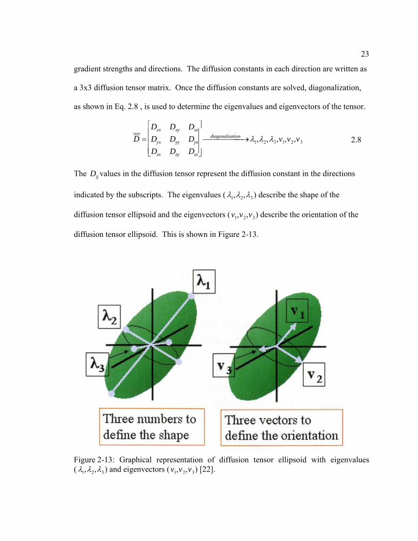
23

gradient strengths and directions. The diffusion constants in each direction are written

a 3x3 diffusion tensor matrix. Once the diffusion constants are solved, diagonalization

as shown in Eq.

as

,

e .

The values in the diffusion tensor represent the diffusion constant in the directions

2.8 , is used to determine the eigenvalues and eig nvectors of the tensor

ij

indicated by the subscripts. The eigenvalues (

D

λ1,λ2,λ3) describe the shape of the

diffusion tensor ellipsoid and the eigenvectors (v1,v2,v3) describe the orientation of the

iffusion tensor ellipsoid. This is shown in Figure 2-13. d

D =Dxx Dxy Dxz

Dyx Dyy Dyz

Dzx Dzy Dzz

⎡

⎢ ⎢ ⎣

⎢ ⎤

⎥ ⎥

⎯ → ⎯ ⎯ ⎯ ⎯ λ1,λ2,λ3,v1,v2,v3

⎦

⎥ diagonalization 2.8

Figure 2-13: Graphical representation of diffusion tensor ellipsoid with eigenvalues ( λ1,λ2,λ3) and eigenvectors (v1,v2,v3) [22].

24

The acquisition of diffusion weighted images (DWI) was described in this

subsection. The next section will describe the basic acquisition of DTI and the

measurement of the diffusion constants shown in Eq. 2.8. It will also briefly descr

some of the most common scalar image types that are calculated using the eigenvalues

and eigenvectors for qMRI.

2.3.2 Acquisition and measurement

dients

and the remaining 6 with diffusion gradients applied in the di icated by the

subscripts in Eq. 2.8. More directions may be added (as long as the directions are not

collinear with respect to each other) for improved calculation of

ibe

As described in the previous section, at least 7 images must be acquired to

determine the diffusion tensor. One image must be acquired without diffusion gra

rections ind

D and the eigenvalues

and eigenvectors. Currently, typical clinical scanners provide DTI sequences with 16

der to a

ust be used. Presently, the most prevalent

sequence used for DTI is the single-shot sp

directions or more. In or cquire DTI with multiple directions in a clinically

acceptable time, fast imaging sequences m

in-echo echo planar imaging (EPI) technique

shown in Figure 2-14 . This is method is preferred because it is fast (< 100 ms per

image) and is relatively insensitive to motion [23].

25

Figure 2-14: A typical single-shot spin-echo EPI sequence used for DTI. Gdiffusion gradient in an arbitrary direction [23].

d is the

Once acquired, a number of methods exist for calculating D [4]. The method that

llows is one of the more common methods and is the one used for the ALS results

presented in Chapter 8. The diffusion tensor is represented as a 6 element column vector

as shown in Eq. 2.9.

For M gradient directions with b > 0, the M×6 gradient encoding matrix is constructed

using the norm 2.10.

sing

fo

[ ]T

alized gradient components, gxi, gyi, and gzi, as shown in Eq.

Another column matrix is formed using the apparent diffusion coefficients (ADC’s)

calculated u Eq. 2.7 as shown in Eq. 2.11.

yzxzxyzzyyxx DDDDDDd ,,,,,= 2.9

2.10

[ ]TDMDD bSSbSSbSSY /)/ln(,,/)/ln(,/)/ln( 21 K= 2.11

⎟⎟⎠

⎜⎜⎝ zMyMzMxMyMxMzMyMxM ggggggggg 222222

⎟⎟⎟⎞

⎜⎜⎜⎛

= zyzxyxzyx

zyzxyxzyx

gggggggggggggggggg

H222222

22222222

22

22

11111121

21

21

MMMMMM

26

D may be estimated using either anAt this point unweighted linear least squares fit as

shown

ollowing estimation of

in matrix notation in Eq. 2.12 or using singular value decomposition (SVD) as

shown in Eq. 2.13 . SVD decomposes a matrix into a product of 3 matrices [24].

( ) YHHHd TT 1−= 2.12

UWVH T SVDby ,= 2.13YUVWd = T1-

F D the eigenvalues and eigenvectors are calculated using

diagonalization as illustrated in Eq. 2.8.

vides many useful quantitative parameters [3]. Among them, fractional

anisotropy (FA) and mean diffusivity (MD) are the most commonly used and reported to

haracterize tissue status. MD is the average diffusivity of the three diagonal diffusion

coefficients as shown in Eq. 2.1

FA is a scalar value that describes the amount of diffusion anisotropy present in a voxel

and is defined in Eq.

DTI pro

c

4.

2.15.

Note that when the diffusion is isotropic λ1 = λ2 = λ3, FA=0. Conversely, when the

diffusion is completely anisotropic in any direction, FA = 1. Also, note that FA and MD

3zzyyxxMD

)( DDD ++= 2.14

[ ])(2

)()(3

)(2)()()(

23

22

21

232

21

23

22

21

213

232

221

λλλλλ

λλλλλλλλλ

++

−+−=

++

−+−+−=

MDMD

FA

2.15)( 2λ +− MD

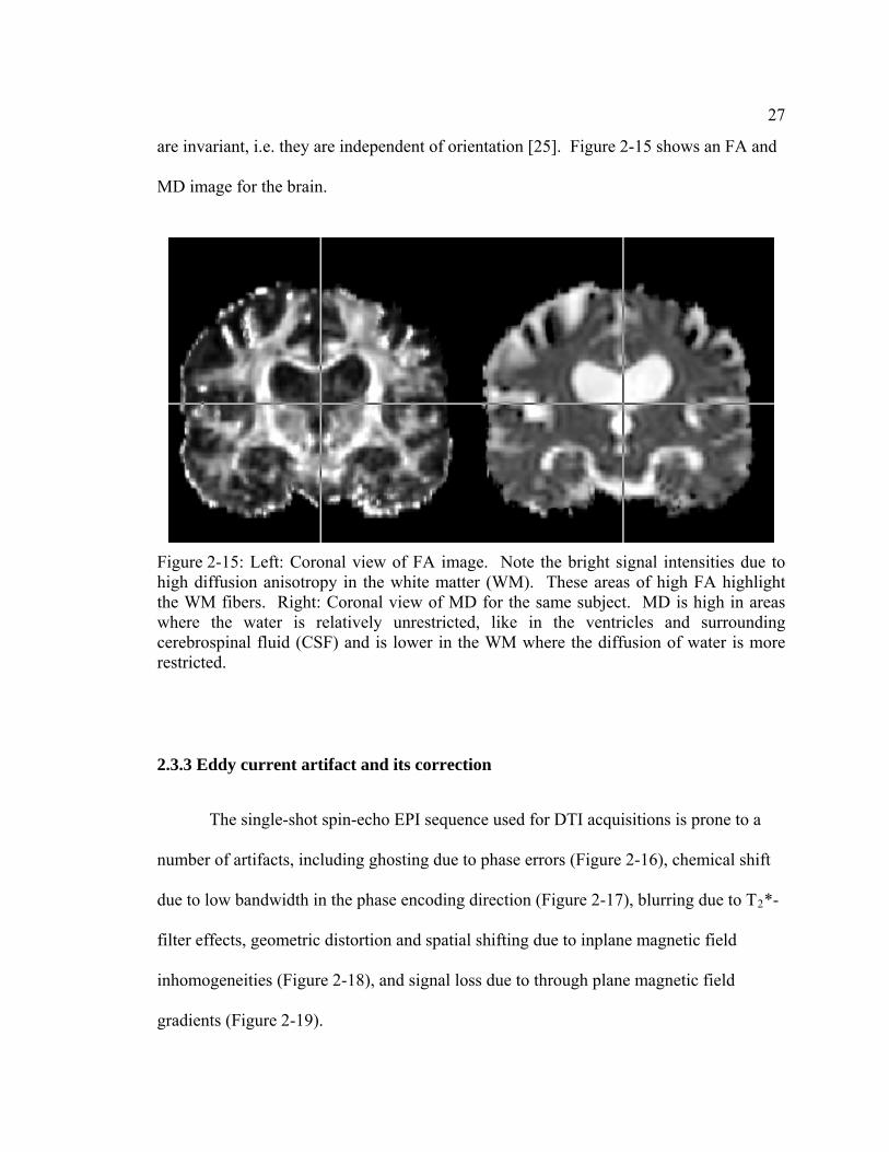
27

are inv ndent of orientation [25]. Figure 2-15 shows an FA and

D image for the brain.

2.3.3 Eddy current artifact

t

ariant, i.e. they are indepe

M

Figure 2-15: Left: Coronal view of FA image. Note the bright signal intensities due tohigh diffusion anisotropy in the white matter (WM). These areas of high FA highlight the WM fibers. Right: Coronal view of MD for the same subject. MD is high in areaswhere the water is relatively unrestricted, like in the ventricles and surroundingcerebrospinal fluid (CSF) and is lower in the WM where the diffusion of water is morerestricted.

and its correction

The single-shot spin-echo EPI sequence used for DTI acquisitions is prone to a

number of artifacts, including ghosting due to phase errors (Figure 2-16), chemical shif

due to low bandwidth in the phase encoding direction (Figure 2-17), blurring due to T2*-

filter effects, geometric distortion and spatial shifting due to inplane magnetic field

inhomogeneities (Figure 2-18), and signal loss due to through plane magnetic field

gradients (Figure 2-19).

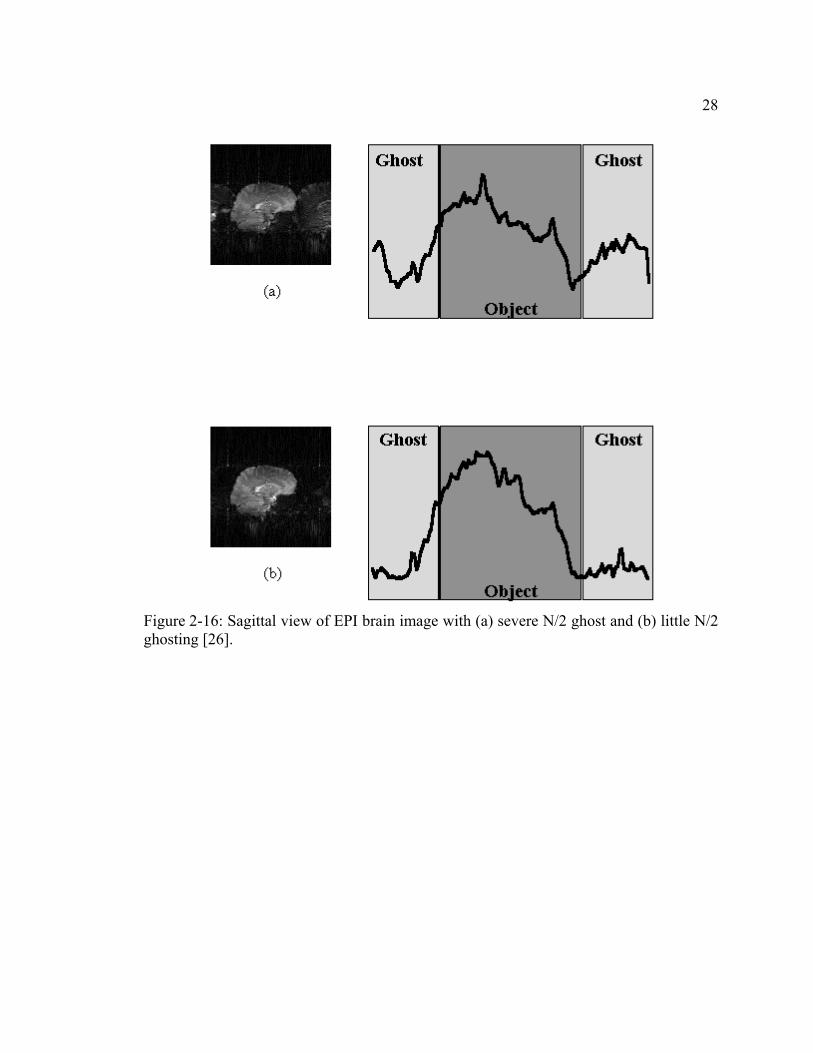
28

Figure 2-16: Sagittal view of EPI brain image with (a) severe N/2 ghost and (b) little N/2 ghosting [26].

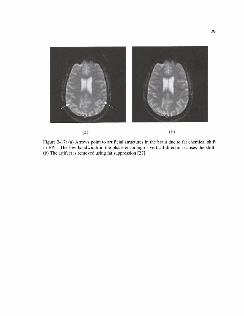
29

Figure 2-17: (a) Arrows point to artificial structures in the brain due to fat chemicalin EPI. The low bandwidth in the phase encoding or vertical direction causes the shift.(b) The artifact is removed using fat suppression [27].

shift

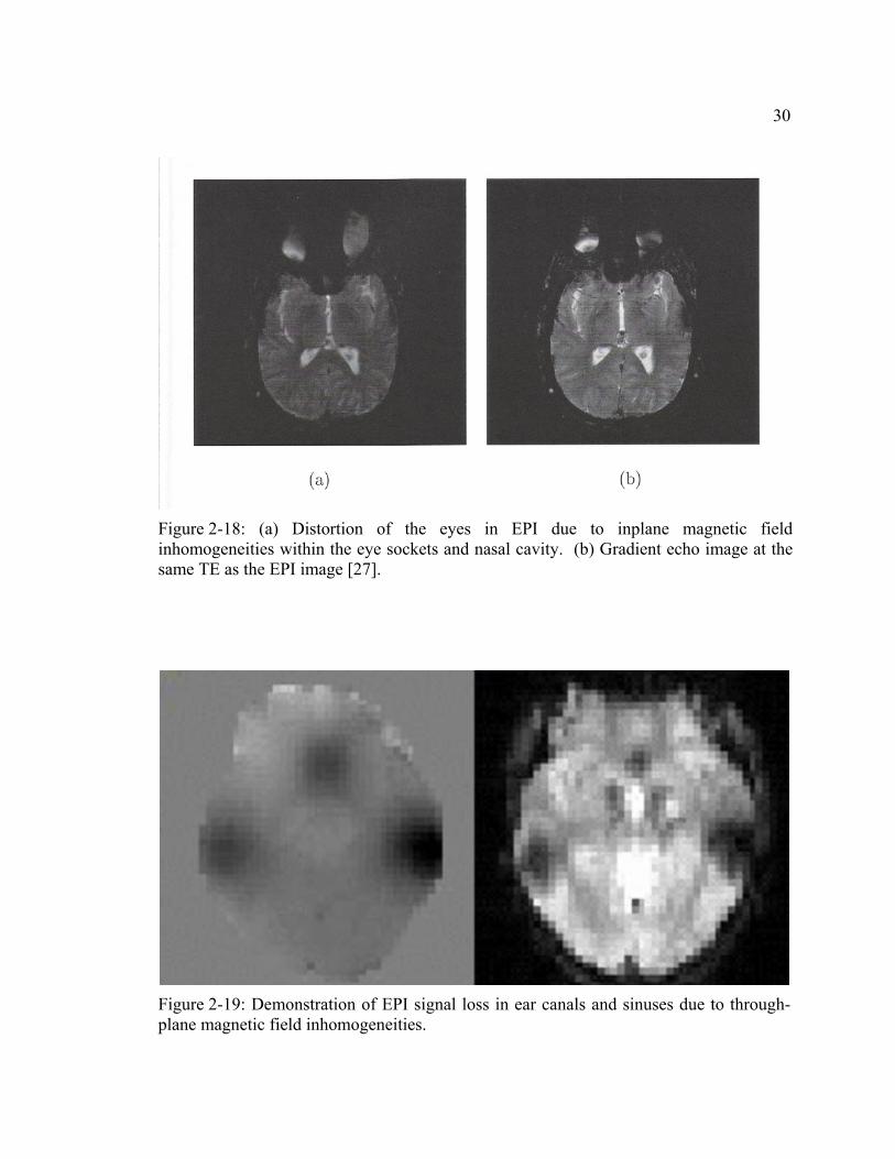
30

Figure 2-18: (a) Distortion of the eyes in EPI due to inplane magnetic fieldinhomogeneities within the eye sockets and nasal cavity. (b) Gradient echo image at thesame T

E as the EPI image [27].

Figure 2-19: Demonstration of EPI signal loss in ear canals and sinuses due to throughplane magnetic field inhomogeneities.

-

31

Spatial shifting of images due to eddy currents is particularly problematic for

DTI. Rapid switching of magnetic field gradients causes formation of eddy currents in

RF coils, RF shields, main magnet components, and the sample being imaged. The

induced currents create time-varying magnetic fields that oppose the applied magnetic

field gradients and can cause the previously demonstrated phase error, geometric

se

distortion, and spatial shifting [27]. In DTI, it is assumed that the preprocessed DWI's

isregistration can occur primarily due to

varying eddy currents produced by the diffusion gradients with different amplitudes and

directions [23].

rrents has been addressed using pre-

emphasis calibration [28], twice-refocused RF spin-echo with two bipolar diffusi

gradient pairs [29], and post-acquisition registration to realign the images [30]. Parallel

MRI minimizes many of the EPI artifacts, but does not eliminate them altogether. For

instance, registration analysis performed on a control subject used in the ALS study

presented in Chapters 6-8 showed that scales and shears were minimal, but voxel shifts in

the phase encoding direction up to 2.5 voxels were detected. As a result of this analysis,

post-acquisition registration-based eddy current correction using FMRIB Software

Library (FSL) [31] was employed for the DTI results used in this thesis. Tcl and C++

tools were developed to automatically correct the images for eddy currents and then

calculate the tensor images, MD, and FA. The source for this tool is located in Appendix

C.

are all properly registered, but considerable m

Removing distortions caused by eddy cu

es on

32


Using DTI the white matter fibers can be vividly visualized in 3D, because the

ments of water molecules are highly ori on of the white matter

A number of biological changes within the brain can be detected including:

Inflammation (localized response to injury or destruction of tissue), edema (large

quantities of abnormal fluids present in intercellular tissue spaces), cell swelling

(abnorm ring

, membrane damage, demyelination (loss of the myelin sheath of the nerve),

cell growth (abnormal formation such as a cyst or a tum r), axonal loss, gliosis (excess of

astroglia in damaged areas of the brain), and axonal reorganization (modification of brain

structure following injury or disease) [21]. It is not always possible to distinguish which

of these pathologic processes is the source of DTI changes observed in neurodegenerative

disease. However, microscopically it has been established that the intact axonal

membrane is the most important determinant of diffusion anisotropy in neural tissue [32].

The myelin sheath only has a small moderating effect on diffusion anisotropy [32].

Furthermore, detectable decreases of diffusion anisotropy typically occur only in areas of

the brain where the anisotropy is normally high [33]. Some disease processes have been

well characterized. For instance, Wallerian degeneration or axonal degeneration due to

axon damage, within the corticospinal tract (CST) is characterized by a reduction in FA

move ented along the directi

fibers [25]. Figure 2-20 shows an example of DTI fiber tracking. Therefore, pathology

that alters the diffusion of water within the white matter should be detectable using DTI.

al enlargement of the cell volume), cell necrosis (morphological changes du

cell death)

o

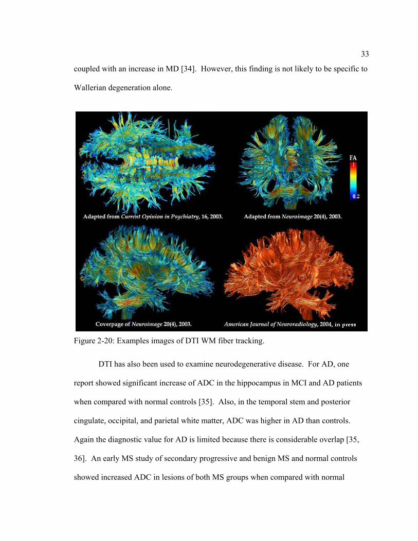
33

coupled with an increase in MD [34]. However, this finding is not likely to be specific to

,

showed increased ADC in lesions of both MS groups when compared with normal

Wallerian degeneration alone.

Figure 2-20: Examples images of DTI WM fiber tracking.

DTI has also been used to examine neurodegenerative disease. For AD, one

report showed significant increase of ADC in the hippocampus in MCI and AD patients

when compared with normal controls [35]. Also, in the temporal stem and posterior

cingulate, occipital, and parietal white matter, ADC was higher in AD than controls.

Again the diagnostic value for AD is limited because there is considerable overlap [35

36]. An early MS study of secondary progressive and benign MS and normal controls

34

controls, but no difference between the two MS groups [37]. A later study showed that

the ADC within lesions of secondary progressive MS patients was significantly higher

than relapsing-remitting MS patients. ADC was significantly higher in both groups when

compared to normal controls [38]. Chapters 5 and 7 will discuss the significance of DTI

in ALS.

2.4 Morphological measurements

Compared to other imaging modalities, MRI provides the best soft tissue contrast

and resolution for the whole-brain. Standard clinical MRI produces images with good

signal-to-noise ratio (SNR) and contrast-to-noise ratio (CNR) at isotropic resolutions

down to 1 mm. At this resolution useful anatomical quantities may be measured for

applications to neurodegenerative disease, brain development, and aging. The following

subsections will briefly cover some of the more useful and common anatomical

measurements and their significance to neurodegenerative disease.

2.4.1 Volume

in the brain

and then multiplying the total number of voxels in the ROI by the product of the image

spacing in the three directions. The real challenge in performing volume measurements

is identification of the ROI, which may be performed manually, automatically, or semi-

automatically. Many software packages exist for performing these three tasks, an

Brain volume is measured by identifying a region of interest (ROI)

35

enumeration of which is outside the scope of this thesis. However, some of the more

common volume measurements and how they are obtained will be described next.

2.4.1.1 Brain parenchyma fraction (BPF)

Brain parenchyma fraction (BPF) is one of the more common brain volume

measurements. BPF is defined in Eq. 2.16.

Here VGM, VWM, VCSF are the whole-brain volumes for GM, WM, and CSF respectively.

BPF accounts for normal whole-brain volume variation amongst normal subjects of the

same age by normalizing the brain parenchyma volume by the intracranial volume.

d VCSF is most often performed by segmenting or labeling the

brain im

Measuring VGM, VWM, an

ages using automatic methods. Once the brain is labeled, the volumes are

calculated as described in Section 2.4.1.

FAST [39], part of FSL [31], is one of the more common automatic brain

segmentation tools. SPM (http://www.fil.ion.ucl.ac.uk/spm/) also provides brain

segmentation tools and is often employed for this purpose. Most automatic tools segm

the brain into the three previously mentioned tissue classes. Automatic brain

segmentation is an area of active research and new techniques and tools appear regularly.

Again, the details of these tools and methods are outside the scope of this thesis.

Figure

ent

2-21 shows a T1-weighted image with the corresponding segmented image.

CSFGM

WMGM

VVVVV

BPF++

+

WM

= 2.16

http://www.fil.ion.ucl.ac.uk/spm/

36

Figure 2-21: Left: Coronal view of T1-weighted image. Right: Same coronal view of image on left, but with overlay image segmented into gray matter (GM), white matter(WM), and cerebrospinal fluid (CSF). GM is red, WM is yellow, and CSF is light blue.

2.4.1.2 Ventricular fraction (VF)

Another volume measurement is ventricular fraction (VF). VF is defined in

Eq. 2.17.

CSFWMGM

VENT

VVVV

VF++

= 2.17

In this case, VVENT is the volume of the lateral ventricles. Measuring VF is slightly more

difficult than BPF, because it involves measuring the volume of the ventricles separate

st approach is to first segment the brain, as described

in Sect e

mechanism for elastic registration (HAMMER)

from the rest of the CSF. The easie

ion 2.4.1.1, and then use semi-automatic region growing segmentation tools, lik

ITK-SNAP [40], to label the ventricles separately. The hierarchal attribute matching

37

(https://www.rad.upenn.edu/sbia/software/) tool can also be used to automatically labe

the ventricles in a segmented image and works well for most brains. Figure

l

)

red to a

2-22 shows

the image in Figure 2-21 with ventricles relabeled using the HAMMER tool.

Figure 2-22: Coronal view of segmented image in Figure 2-21 with the ventriclesrelabeled.

ht blue, and ventricles are dark blue. GM is red, WM is yellow, CSF is lig

2.4.1.3 Voxel-based morphometry (VBM

Voxel-based morphometry (VBM) refers to the process of determining whole-

brain atrophy and volume differences using segmented brain images [41]. Essentially,

VBM is a four-step process. First, the brain images are normalized or registe

standardized brain template. Registration forces all of the brains to have the same shape,

size, and orientation and is described in more detail in Section 2.5.3.1. Second, the

https://www.rad.upenn.edu/sbia/software/

38

registered brain images are segmented into GM, WM, and CSF.1 In the segmented

images MRI image intensities are replaced with a value between 0 and 1, representing the

tissue c

in

.3).

d

tion-based morphometry. The deformation field itself may

also be used to examine deformation differences between subject groups [41]. Figure 2-

putational neuroanatomy and how they are related.

oncentration at any particular voxel. Third the images are smoothed using a

Gaussian smoothing kernel in order to remove small anatomical differences that rema

after registration (Section 2.5.3.2). Finally, the smoothed images are separated into

patient groups and compared, typically, using the general linear model (Section 2.5.3

Using this standard technique, VBM is good for indentifying regions of GM atrophy in

the brain. In addition to the standard technique just described, if the segmented images

are modulated by the determinant of the Jacobian of the non-linear deformation field use

to register the images, regional volume differences may be indentified. This form of

VBM is often called deforma

23 shows the various forms of com

1 The registration and segmentation steps can be reversed or performed simultaneously.

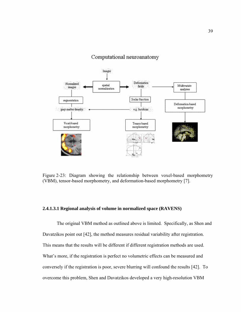
39

Figure 2-23: Diagram showing the relationship between voxel-based morphometry (VBM), tensor-based morphometry, and deformation-based morphometry [7].

2.4.1.3.1 Regional analysis of volume in normalized space (RAVENS)

The original VBM method as outlined above is limited. Specifically, as Shen and

Davatzikos point out [42], the method measures residual variability after registration.

This m d.

solution VBM

eans that the results will be different if different registration methods are use

What’s more, if the registration is perfect no volumetric effects can be measured and

conversely if the registration is poor, severe blurring will confound the results [42]. To

overcome this problem, Shen and Davatzikos developed a very high-re

40

method [42], called regional analysis of volume in normalized space (RAVENS), that

performs registration while taking care to preserve the total amount of tissue after

deformation. RAVENS is physically analogous to the squeezing or stretching of a rubber

information on RAVENS image processing.

object, which changes the density of the rubber to maintain the total mass in the object

(Figure 2-24) [42]. See Chapter 3 for more

Figure 2-24: Orthogonal views of RAVENS image. Higher voxel densities correspond to areas of increased density after warping to an atlas and vice-versa [42].

41

2.4.2 Cortical thickness

Chapter 4 will cover brain cortical thickness measurements in more detail. This

section will serve as a brief overview of cortical thickness measurements using MRI.

Similar to volume, cortical thickness may be measured manually or automatically.

Automatic methods may be lumped into voxel-based methods, surface-based methods, or

voxel/surface hybrid techniques. Figure 2-25 shows surface-based cortical thickness

using the popular freesurfer tool (http://surfer.nmr.mgh.harvard.edu/). Figure 2-26 shows

an example of manual thickness measurements taken along the motor cortex. Measuring

the direction that thickness is measured). Chapter 4 will discuss the

cortical thickness is more challenging than volume due to the problem of topology

(determination of

problem of topology in more detail.

Figure 2-25: Sagittal views of gray/white (left), pial (center), and inflated (right) surfacerepresentations with overlaid cortical thickness measurements [43].

http://surfer.nmr.mgh.harvard.edu/

42

Figure 2-26: Manual measurements of thickness for a patient with primary lateralsclerosis in A and B. Similar thickness in C and D for an age and gender matched control subject. B and D show inflated views of the thickness measurements along the anterior(white arrows) and posterior (black arrows) banks of the primary motor cortex and S1(black arrowheads) [44].


Chapters 5, 6, and 7 cover the significance of BPF, VF, VBM, and cortical

thickness in ALS. VBM has also been used in AD [45-48]. The most common finding is

43

atrophy within the hippocampus. Studies for cortical thickness have also been emplo

for AD [49-51], with findings similar to VBM studies.

yed

2.5 Sta

tively. A more detailed explanation of

statistical parametric mapping (SPM) will be covered in Section 2.5.3. While SPM was

originally developed for functional neuroimaging using positron emission tomography

puted tomography (SPECT), and fMRI, it can be used

for any

in

el-

e

tistical analysis of images

This section will summarize the statistical methods used to analyze qMRI. In

describing the methods, this section will not cover parametric statistics in great detail.

Other methods for comparing quantitative data exist, but are outside the scope of this

thesis and therefore will not be discussed. Sections 2.5.1 and 2.5.2 will briefly touch on

ROI and histogram based approaches respec

(PET), single photon emission com

type of whole-brain statistical analysis. In the case of qMRI using transverse

relaxation parameter maps, DTI, and anatomical measurements, only the second level or

group analysis functions of SPM are useful. Therefore, the summary of SPM included

this chapter will not cover the first level or functional aspects of SPM. Studies that use

SPM for analysis of transverse relaxation parameter maps of the brain are called vox

based relaxometry (VBR) and studies that use DTI scalar images like FA and MD ar

sometimes called voxel-based DTI (VB-DTI).

44

2.5.1 Region of interest (ROI) analysis

ROI’s

hile

ost cases ROI’s are used to study only

one tissue, so the presence of another tissue causes this error [52].

ber of limitations. First, manual creations of ROI

require time to learn. In addition, if multiple raters are employed, each rater tends to

develop their own technique. Therefore, in

insure that the inter-rater variability is low. It is also advisable to look at intra-rate

,

I

Histogram analysis is one way to quantify and compare disease processes for the

whole-brain. In order to perform this type of analysis, the brain must first be segmented

ROI analysis is appropriate for studies where the location in the brain is known

beforehand. The ROI’s can be any shape and size but are typically defined by anatomical

landmarks or structures. In most cases, ROI’s are defined manually or semi

automatically. When creating ROI’s, a compromise exists between creating large

or small ROI’s. Large ROI’s reduce noise but can have more partial volume error w

small ROI’s have more noise and less partial volume error. Partial volume error occurs

when an ROI contains a mixture of tissues. In m

ROI analysis suffers from a num

the case of multiple raters, one needs to

r

variability (repeated measurements from one rater). To circumvent the inter/intra-rater

problem, it is possible to create ROI’s for images that have been registered. In this case

one needs to be aware of the sources of registration error. Another drawback with RO

analysis is the possibility of missing active disease processes in a separate part of the

brain not tagged as the ROI.

2.5.2 Histogram analysis

45

either by tissue or by some sort of pathological entity such as a tumor or legion. Once the

segmentation is performed, histograms can be performed using standard methods and

compared. The disadvantage of using histograms is that the spatial information is lost.

2.5.3 Statistical parametric mapping (SPM)

From the SPM website (http://www.fil.ion.ucl.ac.uk/spm/), SPM refers to the

construction and assessment of spatially extended statistical processes used to test

hypotheses about function or disease within brain imaging data. This process involves,

registration of images to standardized space, smoothing the registered images, and then

testing modeled hypothesis on the image data using the general linear model (GLM) and

the theory of Gaussian random fields (GRF). Each step will be covered in the following

subsections.

2.5.3.1 Registration

Registration of brain image data across subjects is essential for making whole-

brain statistical comparisons. Brain registration is a field of its own and, like brain

segmentation, as a very active area of research. Section 2.5.3.1.1 will describe the basics

of linear affine registration and then Section 2.5.3.1.2 will touch on non-linear

registration.

http://www.fil.ion.ucl.ac.uk/spm/

46

2.5.3.1.1 Affine linear registration

Affine or 12 parameter linear registration is important because it is usually

three-dimensions

3 param

8:

where t e

D matrix

⎥⎦

⎢⎣

⎥⎦⎣⎦⎣

employed as the starting point for non-linear registration techniques. In

eters are needed for rotation, 3 for translation, 3 for scaling, and 3 for skewing

(shearing). In matrix form an affine transform is defined by Eq. 2.1

⎥⎥⎥⎤

⎢⎢⎢⎡

⎥⎥⎥⎤

⎢⎢⎡

=⎥⎥⎤

⎢⎢⎡

′′

⎢⎢

⎥⎥

⎢⎢

′

==)(33321

232221

131211

zyx

tMMtMMMtMMM

yx

xAxTz

y

x

rr

he Mij components are combinations of rotations, scales, and skews, tx, ty, tz ar

the translations in x, y, and z respectively.

For demonstration purposes, it is easier to describe these operations in 2-

form. In 2-D, an affine linear transform only requires 7 parameters. Eq. 2.19 shows the

2-D matrix equation for clockwise rotation of θ about the origin. Figure 2-27 shows the

effect of this transformation on a 2-D slice of the brain.

1100

2.18

⎥⎥⎦⎢

⎢⎣⎥

⎥⎦⎢

⎢⎣

−==1100

0cossin)( yxRxT θθ 2.19

013Mz

⎥⎢⎥⎢rr⎤⎡⎤⎡ 0sincos xθθ

47

Eq. 2.20 shows the matrix equation for translation. Figure 2-28 shows the effect of

translation on a 2-D slice of the brain.

Figure 2-27: Application of rotation transform about the origin to a 2-D slice of the brain [53].

⎥⎥⎥

⎦

⎤

⎢⎢⎢

⎣

⎡

⎥⎥⎥

⎦

⎤

⎢⎢⎢

⎣

⎡==

11000000

)( yx

mm

xMxT y

xrr 2.20

Figure 2-28: Application of x translation (left) and y translation (right) for a 2-D slice of the brain [53].

48

Eq. 2.21 shows the matrix equation for scaling. Figure 2-29 shows the effect of

translation on a 2-D slice of the brain.

2.2

e.

2.21⎥⎥⎥

⎦⎢⎢⎢

⎣⎥⎥⎥

⎦

⎢

⎣ 110000 yrr

⎤⎡⎤

⎢⎢

⎡==

00)(

xs

sxSxT y

x

Eq. 2 shows the matrix equations for skews parallel to the x axis and parallel to the y

axis. Figure 2-30 shows the effect of a skew parallel to the x axis on the 2-D brain slic

the y direction for a 2-D slice of the

brain [53].

⎥

2.22

Figure 2-29: Application of a scale > 1 transform in

⎥⎥⎤

⎢⎢⎢⎡

⎥⎥⎥⎤

⎢⎢⎢⎡

==1100

01001

)( 2 yx

kxKxT yrr

⎥⎥⎥

⎦⎢⎢⎢

⎣⎥⎥⎥

⎦⎢⎢⎢

⎣

==1100

010)( 1 yxKxT rr

⎤⎡⎤⎡ 01 xkx

⎦⎣⎦⎣

49

2-30: Application of a skew transform parallel to the x axis for a 2-D slice of the3].

Figure [5brain

Rotatio

size

after th

y

maxim st function using an optimizer. In addition, an

interpo

ITK So areGuide.pdf

n and translation transformations combined are commonly called rigid-body

transformations because the object being transformed retains its original shape and

e transformation.

In practice linear affine registration requires finding the linear affine transform of

a moving brain image to a fixed brain image. This is most commonly performed b

izing or minimizing some co

lator is required in order to find intensity values in the transformed space. The

ftware Guide (http://www.itk.org/ItkSoftw ) provides explanations

and exa in

learning the basics of linear registration.

mple code for each of these tasks and is an excellent guide for those interested

http://www.itk.org/ItkSoftwareGuide.pdf

50

2.5.3.1.2 Non-linear registration

Non-linear brain registration techniques perform geometric transformations that

be described using simple linear transformations as described in Section 2.5.3.1.1. cannot

vector voxel location that

e

groups; intensity based approaches and geom

rs

a

2.5.3.2

thereby

inferen

reasona th Gaussian field. This

assump oxel size.

3) Smo

Typically non-linear transformations are described using vector deformation fields. A

deformation field is a 3-D image defined by vectors at each

defin the magnitude and direction of transformation for each voxel (see Chapter 3,

Section 3.6 and Figure 3-6). Non-linear brain registration may be lumped into two

etrically based approaches. Chapter 3

cove the non-linear registration technique used for the ALS results in Chapters 6 – 8.

The interested reader is encouraged to read Arthur W. Toga’s book [6] for more

inform tion on non-linear brain registration techniques.

Smoothing

In the context of qMRI used in SPM, smoothing of registered images is required

for 3 reasons: 1) Smoothing the data will make the errors more normally distributed and

ensuring validity of inferences using parametric tests. 2) When making

ces using GRF’s (Section 2.5.3.4), it is assumed that the error terms are a

ble lattice representation of an underlying and smoo

tion requires that the smoothness of the image data is larger than the v

othing reduces registration error [7].

51

2.5.3 General linear model (GLM) .3

e

is

the bra A,

O

possibl tem.

e

almost

I.

desired

The general linear model is a linear statistics model given by Eq. 2.23.

εβ += XY 2.23

wher Y is a matrix with series of multivariate measurements, X is a design matrix, β a

matrix with the estimated values, and ε is the error matrix. For qMRI using SPM, Y

in image data and X is the statistical model (i.e. two-sample, paired, ANOV

ANC VA, full-factorial, etc.). Using GLM and the theory of GRF (Section 2.5.3.4), it is

e to model and test hypotheses using the entire brain as a mass-univariate sys

Figur 2-31 shows how the GLM works for fMRI (first level analysis). The process is

exactly the same for the second level analysis or group analysis that is used for

qMR The difference is that the S parameter is always 1 and the design matrix is the

model instead of the fMRI time course.

52

Figur 2-31: The general linear model (GLM). In fMRI the data can be filtered wtion or residual forming matrix (or a combination) S, le

e ith aconvolu ading to a generalizedlinear odel that includes (intrinsic) serial correlations and applied (extrinsic) f m iltering. S is always 1 for group analysis using qMRI The parameter estimates are obtained in aleast squares sense using the pseudoinverse (denoted by +) (see Eq. 2.12) of the filtered design matrix. Generally an effect of interest is specified by a vector of contrast weightsc that give a weighted sum or compound of parameter estimatesβ ̂referred to as a contrast. The T statistic is simply this contrast divided by its estimated standard error (i.e. square root of its estimated variance). The ensuing T statistic is distributed with ν v degrees of freedom. The equations for estimating the variance of the contrast and the degrees offreedom associated with the error variance are provided in the right-hand panel. Efficiency is simply the inverse of the variance of the contrast. These expressions areuseful when assessing the relative efficiency of experimental designs. The parameterestimates can either be examined directly or used to compute the fitted responses (see lower left panel). Adjusted data refers to data from which estimated confounds havebeen removed. The residuals r is obtained from applying the residual-forming matrix R to the data. These residual fields are used to estimate the smoothness of the component fields of the SPM used in random field theory (see Figure) [7].

53

Two types of inferences are made using SPM: 1) anatomically closed hypotheses

and 2) anatomically open hypotheses.

2.5.3.4.1 Anatomically closed hypotheses

make the

The anatomically open hypotheses test the null hypothesis that there is no effect

anywhere in a specified brain volume. In this case p-value correction is required because

the voxels within the brain are spatially dependent. GRF’s provide a way to correct for

multiple comparisons on spatial data that is analogous to Bonferroni correction using

2.5.3.4 Statistical inferences and theory of Gaussian random fields

Anatomically closed hypotheses are essentially equivalent to an ROI analyses

(Section 2.5.1). In this type of analysis the anatomical region is known a priori.

Therefore no correction for multiple comparisons is required or needed and the

uncorrected p-value associated with the height or extent of the region may be used to test

the hypothesis. However, sometimes it is desirable to examine brain regions that are near

a predicted location. In this case one can pre-specify a small search volume and

appropriate GRF correction or use the uncorrected p-value based on the spatial extent of

the nearest cluster [7].

2.5.3.4.2 Anatomically open hypotheses

54

discrete data. Instead of correcting for the number of voxel comparisons, which can be

over 1million voxels in a high-resolution 1 mm isotropic brain image, GRF corrects for

the number of clusters that is determined by the smoothness of the image. The diagram

in Figure 2-32 provides an overview of this process.

55

Figure 2-32: Schematic illustrating the use of Random Field theory in making inferencesabout SPM's. This schematic deals with a general case of n SPM{T} whose voxels allsurvive a common threshold u (i.e. a conjunction of n component SPM’s). The centrprobability, upon which all voxel, cluster or set-level inferences are made, is the probability P of getting c or more clusters with k or more resels (resolution elements)above this threshold. By assuming that clusters behave like a multidimensional Poissonpoint process (i.e. thdistribution of c is Poisexpected num

al

e Poisson clumping heuristic) P is simply determined. Theson with an expectation that corresponds to the product of the

ber of clusters, of any size, and the probability that any cluster willbigger than k resels. The latter probability is shown using a form for a single Z-variate field constrained by the expected number of resels per cluster (<.> denotes expectation oraverage). The expected number of resels per cluster is simply the expected number o

be

fresels in total divided by the expected number of clusters. The expected number ofclusters is estimated with the Euler characteristic (EC) (effectively the number of blobs minus the number of holes). This estimate is in turn a function of the EC density fostatistic in question (with

r theν degrees of freedom v) and the resel counts. The EC densi

the expected EC per unit of D-dimensional volume of the SPM where the D dimensional volume of the search space is given by the corresponding element in the vector of reselcounts. Resel counts can be thought of as a voluthe smoothness of the SPM’s component fields expressed in term

ty is

me metric that has been normalized bys of the full width at

half maximum (FWHM). This is estimated from the determinant of the variance-covariance matrix of the first spatial derivatives of e, the normalized residual fields r (from Figure XT2-31TX). In this example equations for a sphere of radius θ are given. Φdenotes the cumulative density function for the sub-scripted statistic in question [7].

56

To mak e

set

• Cluster-level inference: the number of activated voxels (i.e., volume) comprising

t (i.e., cluster),

• Peak-level inference: the height of maxima within that cluster.

These p-values are corrected for the multiple dependent comparisons and are based on

the probability of obtaining c, or more, clusters with k, or more, voxels, above a threshold

u in an SPM of known or estimated smoothness [54].

e inferences about regionally specific effects the SPM is thresholded, using som

height and spatial extent thresholds that are specified by the user. Corrected p-values can

then be derived that pertain to various topological features of the excursion set (i.e. sub

of the SPM above threshold shown in Figure 2-33):

• Set-level inference: the number of activated regions (i.e., number of connected

subsets above some height and volume threshold),

a particular connected subse

Figure 2-33: Graphical depiction of the subset of SPM above threshold (connectedexcursions) [54].

57

2.6 References

ain: measuring changes caused by disease," 633.

ley, "Introduction to diffusion tensor imaging mathematics: Part I. Concepts in Magnetic Resonance Part A,

athematics: Part II.

Concepts in Magnetic Resonance Part A, vol. 28A, pp. 123-154, 2006. sley, "Introduction to diffusion tensor imaging mathematics: Part III.

Tensor calculation, noise, simulations, and optimization," Concepts in Magnetic Resonance Part A, vol. 28A, pp. 155-179, 2006.

[5] C. Lenglet, J. S. W. Campbell, M. Descoteaux, G. Haro, P. Savadjiev, D. nder, R. Deriche, G. B. Pike, G. Sapiro, K. Siddiqi, and P. matical methods for diffusion MRI processing,"

NeuroImage, vol. 45, pp. S111-S122, 2009. [6] [7] K. J. Friston, "Imaging Neuroscience - Theory and Analysis," in Human Brain

n, C. J. Price, S. Zeki, J. T. Ashburner, and W. D. Penny, Eds. San Diego, CA: Academic

[8] R. C. Brasch, "Work in progress: methods of contrast enhancement for NMR , pp.

781-789, 1983.

brain ageing and neurodegenerative disorders," Nature Reviews. Neuroscience,

[10] J. P. Wansapura, S. K. Holland, R. S. Dunn, and W. S. Ball, "NMR Relaxation

Imaging, vol. 9, pp. 531-538, 1999. ing

relaxation times and gadolinium-DTPA relaxivity values in human cerebrospinal

[12] H. B. W. Larsson, J. Frederiksen, J. Petersen, A. Nordenbo, I. Zeeberg, O.

9.

l. 43, pp. 697-, 1993.

[1] P. Tofts, "Quantitative MRI of the brWest Sussex, England: John Wiley & Sons Ltd, 2003, p.

[2] P. B. KingsTensors, rotations, and eigenvectors," vol. 28A, pp. 101-122, 2006.

] P. B. Kingsley, "Introduction to diffusion tensor imaging m[3Anisotropy, diffusion-weighting factors, and gradient encoding schemes,"

[4] P. B. King

Wassermann, A. AnwaM. Thompson, "Mathe

A. W. Toga, Brain Warping. San Diego, CA: Academic Press, 1999.

Function, 2nd ed, R. S. J. Frackowiak, K. J. Friston, C. D. Frith, R. J. Dola

Press, 2004, pp. 599-1091.

imaging and potential applications. A subject review," Radiology, vol. 147

[9] L. Zecca, M. B. H. Youdim, P. Riederer, J. R. Connor, and R. R. Crichton, "Iron,

vol. 5, pp. 863-873, 2004.

Times in the Human Brain at 3.0 Tesla," Journal of Magnetic Resonance

[11] M. A. Ibrahim, J. F. Emerson, and C. W. Cotman, "Magnetic resonance imag

fluid," Investigative Radiology, vol. 33, pp. 153-162, 1998.

Henriksen, and J. Olesen, "Assessment of demyelination, edema, and gliosis by invivo determination of T1 and T2 in the brain of patients with acute attack of multiple sclerosis," Magnetic Resonance in Medicine, vol. 11, pp. 337-348, 198

[13] A. Antonini, K. L. Leenders, D. Meier, W. H. Oertel, P. Boesiger, and M. Anliker, "T2 relaxation time in patients with Parkinson's disease," Neurology, vo

58

[14] H. B. W. Larsson, J. Frederiksen, L. Kjær, O. Henriksen, and J. Olesen, "In vivo

sclerosis," Magnetic Resonance in Medicine, vol. 7, pp. 43-55, 1988.

Parkinson's disease measured with magnetic resonance," Movement Disord

[16] J. Vymazal, A. Righini, R. A. Brooks, M. C

determination of T1 and T2 in the brain of patients with severe but stable multiple

[15] F. Q. Ye, P. S. Allen, and W. R. W. Martin, "Basal ganglia iron content in ers,

vol. 11, pp. 243-249, 1996. anesi, C. Mariani, M. Leonardi, and

G. Pezzoli, "T1 and T2 in the Brain of Healthy Subjects, Patients with Parkinson Disease, and Patients with Multiple System Atrophy: Relation to Iron Content," Radiology, vol. 211, pp. 489-495, 1999.

Deniau, R. A. Knight, and J. A. Helpern, brain iron concentrations using T2-weighted and T2*-

weighted MRI at 3 Tesla," Magnetic Resonance in Medicine, vol. 32, pp. 335-

[18]

plications of Diffusion Tensor Imaging," in ition ed, A. W. Toga and J. C. Mazziotta,

Eds. San Diego, CA: Academic Press, 2002, pp. 379-397. [23] X. J. Zhou, "Diffusion Imaging," in Handbook of MRI Pulse Sequences, M. A.

Bernstein, K. F. King, and X. J. Zhou, Eds. Burlington, MA: Elsevier Academic Press, 2004, pp. 830-856.

[24] W. H. Press, S. A. Teukolsky, W. T. Vetterling, and B. P. Flannery, Numerical Recipes: The Art of Scientific Computing, Third ed. Cambridge, MA: Cambridge University Press, 2007.

[25] D. L. Bihan, J.-F. Mangin, C. Poupon, C. A. Clark, S. Pappata, N. Molko, and H. Chabriat, "Diffusion tensor imaging: Concepts and applications," Journal of Magnetic Resonance Imaging, vol. 13, pp. 534-546, 2001.

[26] S. Clare: ‘Functional MRI : Methods and Applications’. Ph.D. Thesis, The University of Nottingham, 1997

[27] E. M. Haacke, R. W. Brown, M. R. Thompson, and R. Venkatesan, Magnetic Resonance Imaging: Physical Principals and Sequence Design. New York, NY: John Wiley & Sons, Inc., 1999.

[17] R. J. Ordidge, J. M. Gorell, J. C. "Assessment of relative

341, 1994. E. Sofic, W. Paulus, K. Jellinger, P. Riederer, and M. B. H. Youdim, "Selective Increase of Iron in Substantia Nigra Zona Compacta of Parkinsonian Brains," Journal of Neurochemistry, vol. 56, pp. 978-982, 1991.

[19] P. J. Basser, "Inferring microstructural features and the physiological state of tissues from diffusion-weighted images," NMR in Biomedicine, vol. 8, pp. 333-344, 1995.

[20] E. O. Stejskal and J. E. Tanner, "Spin diffusion measurements: spin-echo in the presence of a time dependent field gradient," The Journal of Chemical Physics, vol. 42, pp. 288-292, 1965.

[21] C. A. M. Wheeler-Kingshott, G. J. Barker, S. C. A. Steens, and M. A. v. Buchem, "D: the Diffusion of Water," in Quantitative MRI of the brain: measuring changes caused by disease, P. Tofts, Ed. West Sussex, England: John Wiley & Sons Ltd, 2003, pp. 204-256.

[22] S. Mori, "Principles, Methods, and ApBrain Mapping - The Methods, 2nd Ed

59

1128, 2006.

[28] F. Calamante, D. A. Porter, D. G. Gadian, and A. Connelly, "Correction for eddy current induced B0 shifts in diffusion-weighted echo-planar imaging," Magnetic Resonance in Medicine, vol. 41, pp. 95-102, 1999.

[29] T. G. Reese, O. Heid, R. M. Weisskoff, and V. J. Wedeen, "Reduction of eddy-current-induced distortion in diffusion MRI using a twice-refocused spin echo," Magnetic Resonance in Medicine, vol. 49, pp. 177-182, 2003.

[30] C. Poupon, C. A. Clark, V. Frouin, J. Régis, I. Bloch, D. Le Bihan, and J. F. Mangin, "Regularization of Diffusion-Based Direction Maps for the Tracking of Brain White Matter Fascicles," NeuroImage, vol. 12, pp. 184-195, 2000.

[31] S. M. Smith, M. Jenkinson, M. W. Woolrich, C. F. Beckmann, T. E. J. Behrens, H. Johansen-Berg, P. R. Bannister, M. De Luca, I. Drobnjak, and D. E. Flitney, "Advances in functional and structural MR image analysis and implementation as FSL," NeuroImage, vol. 23, pp. S208-S219, 2004.

[32] B. Christian, "The basis of anisotropic water diffusion in the nervous system - a technical review," NMR in Biomedicine, vol. 15, pp. 435-455, 2002.

[33] M. Cosottini, M. Giannelli, G. Siciliano, G. Lazzarotti, M. C. Michelassi, A. Del Corona, C. Bartolozzi, and L. Murri, "Diffusion-Tensor MR Imaging of Corticospinal Tract in Amyotrophic Lateral Sclerosis and Progressive Muscular Atrophy," Radiology, vol. 237, pp. 258-264, 2005.

[34] C. Pierpaoli, A. Barnett, S. Pajevic, R. Chen, L. Penix, A. Virta, and P. Basser, "Water Diffusion Changes in Wallerian Degeneration and Their Dependence on White Matter Architecture," NeuroImage, vol. 13, pp. 1174-1185, 2001.

[35] K. Kantarci, C. R. Jack, Jr., Y. C. Xu, N. G. Campeau, P. C. O'Brien, G. E. Smith, R. J. Ivnik, B. F. Boeve, E. Kokmen, E. G. Tangalos, and R. C. Petersen, "Mild Cognitive Impairment and Alzheimer Disease: Regional Diffusivity of Water," Radiology, vol. 219, pp. 101-107, 2001.

[36] R. B. Schwartz, "Apparent Diffusion Coefficient Mapping in Patients with Alzheimer Disease or Mild Cognitive Impairment and in Normally Aging Control Subjects: Present and Future," Radiology, vol. 219, pp. 8-9, 2001.

[37] M. A. Horsfield, M. Lai, S. L. Webb, G. J. Barker, P. S. Tofts, R. Turner, P. Rudge, and D. H. Miller, "Apparent diffusion coefficients in benign and secondary progressive multiple sclerosis by nuclear magnetic resonance," Magnetic Resonance in Medicine, vol. 36, pp. 393-400, 1996.

[38] A. C. Scanderbeg, F. Tomaiuolo, U. Sabatini, U. Nocentini, M. G. Grasso, and C. Caltagirone, "Demyelinating Plaques in Relapsing-remitting and Secondary-progressive Multiple Sclerosis: Assessment with Diffusion MR Imaging," American Journal of Neuroradiology, vol. 21, pp. 862-868, 2000.

[39] Y. Zhang, M. Brady, and S. Smith, "Segmentation of brain MR images through a hidden Markov random field model and the expectation-maximization algorithm," IEEE Transactions on Medical Imaging, vol. 20, pp. 45-57, 2001.

[40] P. A. Yushkevich, J. Piven, H. C. Hazlett, R. G. Smith, S. Ho, J. C. Gee, and G. Gerig, "User-guided 3D active contour segmentation of anatomical structures: Significantly improved efficiency and reliability," NeuroImage, vol. 31, pp. 1116-

60

[41] NeuroImage, vol. 11, pp. 805-821, 2000.

Preserving Deformations and HAMMER Elastic Registration," NeuroImage, vol.

[43] B. Fischl and A. M. Dale, "Measuring the thickness of the human cerebral cortex

Sciences of the United States of America, vol. 97, pp. 11050-11055, 2000. rtex

in Primary Lateral Sclerosis," American Journal of Neuroradiology, vol. 28, pp.

[45] J. C. Baron, G. Chetelat, B. Desgranges, G. Perchey, B. Landeau, V. de la

Based Morphometry in Mild Alzheimer's Disease," NeuroImage, vol. 14, pp. 298-

[46] G. B. Frisoni, C. Testa, A. Zorzan, F. Sabattoli, A. Beltramello, H. Soininen, and

voxel based morphometry," Journal of Neurology, Neurosurgery, and Psychiatry,

[47] G. B. Karas, E. J. Burton, S. A. R. B. Rombouts, R. A. van Schijndel, J. T.

"A comprehensive study of gray matter loss in patients with Alzheimer's disease

2003.

Jiang, "Voxel-based detection of white matter abnormalities in mild Alzheimer

[49] J. P. Lerch, J. C. Pruessner, A. Zijdenbos, H. Hampel, S. J. Teipel, and A. C. y

Computational Neuroanatomy," Cerebral Cortex, vol. 15, pp. 995-1001, 2005. w, J. P. Lerch, A. C. Evans, A. E. Dorr, and N. J. Kabani,

"Spatial patterns of cortical thinning in mild cognitive impairment and Alzheimer's disease," Brain, vol. 129, pp. 2885-2893, 2006.

[51] B. C. Dickerson, A. Bakkour, D. H. Salat, E. Feczko, J. Pacheco, D. N. Greve, F.

ptomatic Amyloid-Positive Individuals," Cerebral Cortex, p. doi:10.1093/cercor/bhn113, 2008.

[52] P. S. Tofts, "The Measurement Process: MR Data Collection and Image Analysis," in Quantitative MRI of the brain: measuring changes caused by disease, P. Tofts, Ed. West Sussex, England: John Wiley & Sons Ltd, 2003, pp. 17-54.

J. Ashburner and K. J. Friston, "Voxel-Based Morphometry--The Methods,"

[42] D. Shen and C. Davatzikos, "Very High-Resolution Morphometry Using Mass-

18, pp. 28-41, 2003.

from magnetic resonance images," Proceedings of the National Academy of

[44] J. A. Butman and M. K. Floeter, "Decreased Thickness of Primary Motor Co

87-91, 2007.

Sayette, and F. Eustache, "In Vivo Mapping of Gray Matter Loss with Voxel-

309, 2001.

M. P. Laakso, "Detection of grey matter loss in mild Alzheimer's disease with

vol. 73, pp. 657-664, 2002.

O'Brien, P. h. Scheltens, I. G. McKeith, D. Williams, C. Ballard, and F. Barkhof,

using optimized voxel-based morphometry," NeuroImage, vol. 18, pp. 895-907,

[48] S. Xie, J. X. Xiao, G. L. Gong, Y. F. Zang, Y. H. Wang, H. K. Wu, and X. X.

disease," Neurology, vol. 66, pp. 1845-1849, 2006.

Evans, "Focal Decline of Cortical Thickness in Alzheimer's Disease Identified b

[50] V. Singh, H. Chertko

Grodstein, C. I. Wright, D. Blacker, H. D. Rosas, R. A. Sperling, A. Atri, J. H. Growdon, B. T. Hyman, J. C. Morris, B. Fischl, and R. L. Buckner, "The Cortical Signature of Alzheimer's Disease: Regionally Specific Cortical Thinning Relates to Symptom Severity in Very Mild to Mild AD Dementia and is Detectable in Asym

61

, Registration, Motion Correction and EPI Distortion," Oxford University, 2008.

[54]

[53] FMRIB, "FSL & Freesurfer Course: Brain Extraction

G. Flandin and K. J. Friston, "Statistical parametric mapping (SPM)," Scholarpedia, vol. 3, p. 6232, 2008.

Chapter 3

Software Tool for Automated MRI Post-processing on a Supercomputer (STAMPS)

3.1 Introduction

In order to improve whole-brain registration (Chapter 2, Section 2.5.3.1) and

reduce subsequent registration errors for SPM, a software tool for automated MRI Post-

processing on a supercomputer (STAMPS) was developed. The details of STAMPS are

described in a journal article recently accepted for publication [1]. Figure 3-1 shows the

main work-flow for STAMPS. STAMPS automates, serially or in parallel on a

supercomputer, the task of non-linearly registering one brain image to another, generating

st, HAMMER is a freely available

(https:/

RAVENS maps, and anatomically labeling a brain image using an atlas with predefined

labels. STAMPS uses HAMMER [2] as the non-linear registration tool. As stated in [1],

HAMMER was chosen for four reasons. Fir

/www.rad.upenn.edu/sbia/software/index.html) non-linear brain registration tool

designed for high-accuracy in anatomical alignment. Second, HAMMER is fast and

stable for a sophisticated non-linear registration tool. Third, as shown in Figure 3-2

er 2,

, it

registered brain images well thus reducing subsequent registration errors for SPM.

Finally, it supported the generation of RAVENS [3] images as described in Chapt

Section . 2.4.1.3.1

https://www.rad.upenn.edu/sbia/software/index.html

63

Figure 3-1: Post-processing in STAMPS for T -weighted images [1]. 1

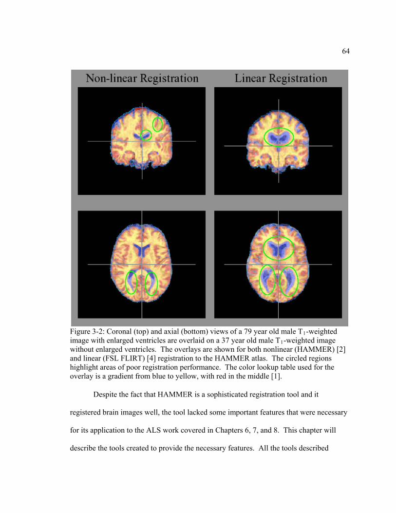
64

Figure 3-2: Coronal (top) and axial (bottom) views of a 79 year old male T1-weighted image with enlarged ventricles are overlaid on a 37 year old male T -weighted image without enlarged ventricles. The overlays are shown for both nonlinear (HAMMER) [2]and linear (FSL FLIRT) [4] registration to the HAMMER atlas. The circled regions highlight areas of poor registration performance. The color lookup table used for the overlay is a gradient from blue to yellow, with red in the middle [1].

1

Despite the fact that HAMMER is a sophisticated registration tool and it

for its application to the ALS work covered in Chapters 6, 7, and 8. This chapter will

describe the tools created to provide the necessary features. All the tools described

registered brain images well, the tool lacked some important features that were necessary

65

herein were created in C++ using a combination of ITK (www.itk.org) and or VTK

(

www.vtk.org) as the foundation. These tools were chosen because they provide readers

for common medical image file formats, have support for image iterators, provide an

mage processing filters, and use a pipeline architecture for

connecting the output of one filter to the input of another filter or to an image writer.

3.2 Con

registra on. As noted

previou

brain atlas. HAMMER can use any labeled brain atlas to perform the labeling by

registration. In many instances the freely available labeled brain atlases include only the

original MR image and the anatomically label atlas, which has no labels for GM, WM,

and CSF. The International Consortium for Brain Mapping (ICBM) Single Subject MRI

Anatomical Template

(http://www.loni.ucla.edu/ICBM/Downloads/Downloads_ICBMtemplate.shtml

extensive library of common i

vert labeled atlas to tissue segmented atlas

HAMMER relies on brain images that have been segmented into GM, WM, and

CSF during the registration process. This is atypical, as most of the current brain image

tion tools use the MR intensities themselves to compute the registrati

sly, HAMMER supports brain labeling of a target brain image using a labeled

) is an

example of a labeled atlas that does not provide GM, WM, and CSF labels. Furthermore,

it was discovered that the anatomically labeled atlas and GM, WM, and CSF labeled

image provided with HAMMER were not in good agreement. Therefore, a tool was

needed to convert the detailed anatomical labeled atlases to a generic GM, WM, and CSF

atlas. Appendix D.1 lists the source for this tool.

http://www.itk.org/

http://www.vtk.org/

http://www.loni.ucla.edu/ICBM/Downloads/Downloads_ICBMtemplate.shtml

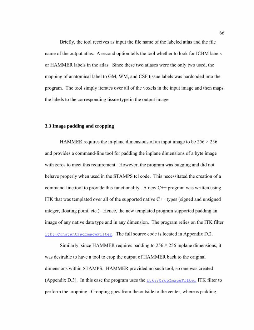
66

Briefly, the tool receives as input the file name of the labeled atlas and the file

name of the output atlas. A second opt tool whether to look for ICBM labels

mapping of anatomical label to GM, WM F tissue labels was hardcoded into the

program. The tool simply iterates over all of the voxels in the input image and then maps

the labels to the corresponding tissue type in the output image.

image

upported native C++ types (signed and unsigned

integer, floating point, etc.). Hence, the new templated program supported padding an

image of any native data type and in any dimension. The program relies on the ITK filter

itk::ConstantPadImageFilter

ion tells the

or HAMMER labels in the atlas. Since these two atlases were the only two used, the

, and CS

3.3 Image padding and cropping

HAMMER requires the in-plane dimensions of an input image to be 256 × 256

and provides a command-line tool for padding the inplane dimensions of a byte

with zeros to meet this requirement. However, the program was bugging and did not

behave properly when used in the STAMPS tcl code. This necessitated the creation of a

command-line tool to provide this functionality. A new C++ program was written using

ITK that was templated over all of the s

. The full source code is located in Appendix D.2.

Similarly, since HAMMER requires padding to 256 × 256 inplane dimensions, it

was desirable to have a tool to crop the output of HAMMER back to the original

dimensions within STAMPS. HAMMER provided no such tool, so one was created

(Appendix D.3). In this case the program uses the itk::CropImageFilter ITK filter to

perform the cropping. Cropping goes from the outside to the center, whereas padding

http://www.itk.org/Doxygen/html/classitk_1_1ConstantPadImageFilter.html

http://www.itk.org/Doxygen/html/classitk_1_1CropImageFilter.html

67

goes from the center out. In both cases, the code is approximately the same as shown in

the following code snippets for the X dimension:

0] = (x-size[0])/2; upperfactors[0] = (x-size[0])/2 + (x-size[0])%2; // C lowerCropSize[0] = (size[0]-x)/2;

Here is the input image X dimension size and is the new cropped or padded

stance,

es intensity outliers from the image by applying a lower

and upper threshold to the im

vtkImageStatistics

itk::ThresholdImageFilter

// Padding. lowerfactors[

ropping.

upperCropSize[0] = (size[0]-x)/2 + (size[0]-x)%2;

size[0] x

dimension size.

3.4 Intensity normalization

MR image intensities for a given scan sequence are highly variable. For in

image artifacts like hyperintense spikes due to physiological noise are common.

Therefore MR image intensities for standard clinical anatomical images cannot be relied

upon for direct quantitative analysis. To allow direct quantitative comparison of

registered standard anatomical MR images, a simple intensity normalization program was

created. The program first remov

age that is plus or minus three standard deviations from the

average image intensity. When determining the average and variance of the image

intensities, the zeros in the image are ignored. A previously implemented statistics

calculator developed in VTK, (Appendix D.4 and D.5), was used

to calculate these values. The ITK filter, , was used to

threshold the image after determination of the upper and lower threshold values. After

applying the threshold to the image, the image is scaled (using

http://www.itk.org/Doxygen/html/classitk_1_1ThresholdImageFilter.html

68

itk::ShiftScaleImageFilter) such that the maximum intensity value is mapped to

32760. This number is just below the maximum 16 bit signed integer value of 32767.

The final output image is then saved as a 16 bit signed integer binary image. The

complete source code is located in Appendix D.6.

3.5 RAVENS normalization

By definition, the voxel intensities of the RAVENS image set (i.e. the GM, WM

and ventricle (VENT) RAVENS images) sum to the patient’s segmented brain volume

prior to the generation of the RAVENS image. The sum is on the order of 1 × 10

,

6 and

mages were generated using 33 T1-weighted images taken

from an ongoing MRI study of AD. A m

varies across subjects. For whole-brain group SPM of RAVENS images, this variation in

subject brain volume introduces a whole-brain volume bias as demonstrated in Figure 3-

3. In this analysis, RAVENS i

ultiple-regression model, using subject age and

whole-brain volume as covariates, was used.

http://www.itk.org/Doxygen/html/classitk_1_1ShiftScaleImageFilter.html

69

Figure 3-3: Whole-brain SPM of 33 RAVENS white matter (WM) images. A multipleregression model using whole-brain volume and age as covariates was used. The

statistics maps were obtained using a false discovery rate (FDR) of 0.05 and 0 voxelextent.

70

As seen in Figure 3-3, a significant relationship between RAVENS WM intensity

and whole-brain volume exists throughout much of the image. These results demonstrate

that whole-brain volume should be included in statistical analyses as a confounding

effect. However, doing so reduces the degrees of freedom for subsequent statistical tests.

So, to remove patient brain volume as a bias from RAVENS images for subsequent

voxel-based analysis, STAMPS provides an option for normalizing the RAVENS image

set such that each patient would have the same sum. The source code for the program

that acc ut the

may be

omplishes this task is listed in Appendix D.7. The program receives as inp

RAVENS image set and outputs normalized versions of each image. Normalized in this

cases means, the sum of the intensities of the RAVENS image set is 1. If the optional

scale factor is supplied, the normalized intensities for the image set will be multiplied by

the scale factor. For STAMPS, the scale factor is 200000000.2 This scale factor puts the

RAVENS image set intensities in the 0 to 255 integer range so that the images

saved as unsigned byte images. Normalizing the RAVENS images in this fashion

eliminates the confounding effect of whole-brain volume while still preserving the age

effect as seen in Figure 3-4.

2 This value was determined empirically to generate the integer intensity images described in the text.

71

Figure 3-4: Whole-brain SPM of 33 normalized RAVENS white matter (WM) images. Amultiple regression model using whole-b

rain volume and age as covariates was used. The statistics maps were obtained using a false discovery rate (FDR) of 0.05 and 0 voxel extent.

72

3.6 Apply HAMMER deformation field to any data type

Lack of support for warping images of any data type is one of the major

limitations of HAMMER. Currently, HAMMER only supports warping of byte images.

Many of the qMRI images are stored as 32 bit floating point. To overcome this

shortcoming, a program was developed that applies the HAMMER generated

deformation field to an image of any native C++ supported data type. This was

accomplished using templated functions and ITK template classes. The

itk::WarpImageFilter is used to apply a deformation field to an input volume, using

the image spacing from a reference image. The HAMMER deformation field is a 3D

volume with a 3D vector at each voxel location that dictates the magnitude and direction

of deformation for that voxel. Figure 3-5 shows a graphical representation of a

HAMMER deformation field midway through the volume.

http://www.itk.org/Doxygen/html/classitk_1_1WarpImageFilter.html

73

Figure 3-5: Axial view of a HAMMER deformation field midway through the volume. to the magnitude of the vector at each voxel location. 3D arrow

glyphs demonstrate the magnitude and direction of deformation. The faint outline of thebrain m

The color is mapped

ay be seen in the center of the slice.

HAMMER stores the vector components of a deformation field in Y, X, and Z

format instead of the typical X, Y, and Z format used by most other programs; includin

ITK. ITK lacks a filter for reordering vector components, so a simple vector compon

reordering filter, itk::VectorReorderComponentsImageFilter, was developed to

accomplish this task. The source code for this filter is located in Appendix

g

ent

rrect deformation field with the vector components reordered in

X, Y, and Z format.

D.8.

Figure 3-6 shows the co

74

Figure 3-6: Axial view of a corrected HAMMER deformation field midway through th

arrow glyphs demonstrate the magnitude and direction of deformation. The vecto

evolume. The color is mapped to the magnitude of the vector at each voxel location. 3D

rcomponents of the deformation were reordered from Y, X, Z format to X, Y, Z format foruse in ITK.

Validation of the program was accomplished by subtracting a byte image

deformed by HAMMER with a byte image deformed by the new tool. The resultant

image volume was zero for each voxel location. The source code for this program is

located in Appendix D.9.

75

3.7 Labeled ROI statistics

HAMMER provides a p l for calculating the volu

labels after an im led using the supplied labeled atlas. lies

the name of the labeled image volume and a text file containing a list of label indexes for

which the volume will be calcu The tool returns the volum x in

a text file. Unfortunately, this list does not contain the descriptive of the

anatomical labels and is therefore difficult to use for subsequent ROI analysis. To

overcome this problem an im ved version of this tool was created. The source code for

this program is listed in Appendix D.12. It also utilizes the vtkImageStatistics class

found in Appendices D.4 and 5.

The new tool is capable of multiple outputs depending on the inputs and options

supplied. It takes as input a subject image, a label image produced using HAMMER, and

e label description file. Without supplying any of the optional input parameters, it

outputs

el

rimitive too me of anatomical

age has been labe The user supp

lated. e for each label inde

names

pro

D.

th

a comma separated value (csv) text file that lists the voxel frequency, arithmetic

mean, variance, median, first quartile, third quartile, maximum, and minimum of the

input subject image voxel intensities for each anatomical label that exists in the label

image. If the -T option is supplied, the program will treat the input subject image as a

thickness image (see Chapter 4) and only the average thickness (as calculated using

Eq. 4.1) will be output in a csv text file. If the -V option is specified, the program will

output the volume information for each brain region in a csv text file instead of the vox

statistics. In this case, the input subject image file must be the segmented image in order

to calculate the total intracranial volume for brain region volume normalization. In all

76

the cases, the csv text file contains the anatomical descriptions of the brain regions to

simplify statistical analysis of the data.

For the no option and –T option scenarios, a new VTK filter,

vtkImageComparison (Appendices D.10 and D.11), was created to aid in the

identification of brain regions within the labeled image. vtkImageComparison can

receive 1 or 2 input images and performs greater than, less than, greater than equal, less

than equal, and equal comparisons of a constant across the entire image for the single

input case or between images in the 2 input case. The filter also provides an option for

changing the “true” value from the default of 1 to some other value. For the described

program, vtkImageComparison is used in the single input case. The index label is

as one of the inputs to vtkImageMask

assigned as the constant to compare for equality across the image. If a voxel is equal to

the constant, it assigned the value of 1, otherwise zero. The output of

vtkImageComparison is assigned . The other input

vtkImageMaskto is the subject input image. At this point the intensity summary

statistics or the average thickness may be com uted from the output of vtkImageMaskp .

3.8 References

ng, "STAMPS: software tool for automated MRI post-processing on a supercomputer," Computer Methods and Programs in

[2] D. Shen and C. Davatzikos, "HAMMER: hierarchical attribute matching .

21, pp. 1421-1439, 2002.

[1] D. C. Bigler, Y. Aksu, and Q. X. Ya

Biomedicine, vol. Accepted for Publication, 2009.

mechanism for elastic registration," IEEE Transactions on Medical Imaging, vol

http://www.vtk.org/doc/nightly/html/classvtkImageMask.html



77

Using the RAVENS Maps: Methods and Validation Using Simulated

[4] M. Jenkinson and S. Smith, "A global optimisation method for robust affine 001.

[3] C. Davatzikos, A. Genc, D. Xu, and S. M. Resnick, "Voxel-Based Morphometry

Longitudinal Atrophy," NeuroImage, vol. 14, pp. 1361-1369, 2001.

registration of brain images," Medical Image Analysis, vol. 5, pp. 143-156, 2

Chapter 4

An Efficient Voxel-based Method for Automatic Estimation of Thickness in Medical Images

4.1 Abstract

ethod for automatically estimating thickness in binary-labeled medical

images

s

med using two

nthetically generated ellipsoids. Utilization for medical image processing is

demonstrated with magnetic resonance images of the brain and knee. These experimental

results show excellent performance for estimating thickness and suggest that this method

is simple and useful for quantifying and visualizing the thickness of anatomical structures

A voxel-based m

using the Euclidean distance transformation (EDT) is presented. The method is

model-independent, less calculation-intensive than surface-based techniques, and thu

fast for processing typical medical images. Validation is perfor

sy

in medical images.

79

4.2 Introduction

In the field of medical imaging, high resolution three-dimensional (3-D) volume

images are frequently acquired in order to evaluate disease and injury. Current computed

tomography (CT) and MRI systems are capable of producing human images with 0.35

mm to 1 mm isotropic spatial resolution. Useful quantitative measurements of

anatomical structures with sizes on the order of this resolution or larger are routinely

extracted from these images. In particular, the measurement of thickness of a given

cartilage thickness in MRI is used for monitoring drug efficacy in osteoarthritis [2].

Finally, femur cortical thickness measurements derived from CT are used to assess

s can be

.

r

d as a

anatomical or pathological structure is important for diagnosing, monitoring, and

assessing disease and injury. For example abnormal cortical thickness was detected in

individuals with Williams Syndrome in MRI [1]. Also, measurement of knee articular

healing after femur fractions [3].

Techniques for measuring the thickness of a structure of interest in image

organized into two groups: surface-based methods and voxel-based methods. In both

methods some form of image segmentation must be performed as a preprocessing step

The surface-based methods use the segmented image to create two mesh surfaces from

which the thickness is measured. Surface-based methods are generally more useful fo

measuring the thickness of image objects that have an inner and outer boundary an

result tend to be model-dependent. Their main advantage is that they tend to maintain the

80

topology of the surfaces. Voxel-based methods calculate the thickness using image data

without the need to create surface meshes. These methods tend to be model-independen

and have the benefit of voxel-to-voxel correspondence with the original image data. The

t

ain disadvantage is that they usually take on an arbitrary topology.

measured by either measuring the distance to the closest point from one surface to the

other, or by following the surface normal vector of one surface to the other. The

f these techniques are preservation of the cortical surface topology and

increas

ces are that they do not intersect with each

other and are approximately parallel to one another. Thickness is calculated by

measuring the lengths between these equipotential surfaces. Yezzi and Prince [9]

generalized this technique and applied it to myocardium, cortical gray matter, and tibial

cartilage. Unlike the method of Jones et al., this generalized method is model-

independent; however the method requires the selection of two surfaces, which can be

m

Many of the surface-based thickness measurement techniques were developed

specifically for the measurement of brain cortical thickness from MRI [4-7]. These

methods first locate the gray and white matter boundary and then expand a deformable

surface until it locates the gray matter and cerebrospinal fluid boundary. Thickness is

advantages o

ed thickness accuracy and precision, but at the expense of model-dependency and

increased processing time.

Another semi-surface-based approach was developed by Jones and colleagues [8].

The method measures brain cortical thickness by applying a solution of Laplace’s

equation between the white matter and gray matter surfaces. The solution to Laplace’s

equation creates layers of equipotential surfaces that flow from one surface to the other

surface. The advantages of equipotential surfa

81

difficult to define for some solid objects such as cartilage. More recently, a new

technique was developed that extends the method by Jones et al to account for buried

cortex within the sulci [10].

Kauffman et al. [11] developed a novel way to measure thickness of cartilage in

MRI by fitting the cartilage surfaces to a geometric model. The cartilage surfaces were

located

ative search

algorithm was employed to measure thickness from the inner boundary offset-map to the

outer-surface offset-map. The ability to register the cartilage surfaces for longitudinal

MRI studies is the main advantage to using this technique. Again, the disadvantage with

this me

ted by computing the

ecause

sently, most voxel-based thickness measurements are performed using an

image distance transform [13-15], which operates on binary image data. Stammberger et

using a two-dimensional active-contour algorithm. By projecting the contour

points to the geometric model “offset-maps” were generated. A 3-D iter

thod is model-dependence, as the geometric model used to generate the offset-

maps must be similar in shape to the extracted surface.

Another surface-based tool for measuring cartilage thickness in MRI was

developed by Tang et al. [12]. Directional gradient vector flow snakes were used to

locate the tibial bone-cartilage, tibial cartilage, talar cartilage, and talar bone-cartilage

surfaces. Average surfaces were created and thickness was compu

distance along the normal vector of one average surface to the other average surface. As

described this approach is applicable to cartilage thickness measurements only b

the cartilage boundary extraction works on a slice-by-slice basis, using the tracking

results from the previous slice. In cases where the contour shape changes dramatically

from slice-to-slice, as in the brain, this approach is difficult to apply.

Pre

82

al. [16] segmented articular cartilage slice-by-slice using a region growing algorithm, and

ffers from the same drawback as the

technique by Yezzi and Prince in that a surface must be specified in order to measure the

Saha and Wehrli [17] used a novel “fuzzy distance transform” to measure

thickne

then applied a 3-D Euclidean distance transformation (EDT) to the bone-cartilage surface

in order to measure the distance between the bone-cartilage surface and the cartilage

surface. This ensures that the thickness is measured normal to the bone-cartilage surface.

Although this method is model-independent, it su

thickness.

ss in trabecular bone. Average thickness is measured by sampling the fuzzy

distance values along the medial axis or skeleton of the image object. Saha and Wehrli

compared their technique with another EDT based method by Hildebrand and

Rüegsegger [18]. Hildebrand and Rüegsegger used a standard EDT that is applied to the

binary object and then the volume-weighted mean thickness and the thickness

distribution are measured by fitting maximal spheres along the “distance ridge.” The

distance ridge was defined as the set of the center points of all nonredundant spheres,

which is equivalent to the medial axis of the structure. The theory of medial

representation of image data and spheres has been well described and applied to shape

analysis and segmentation [19, 20].

Introduced in this chapter is a model-independent voxel-based method to

automatically estimate the thickness of segmented image objects. Similar to the method

of Hildebrand and Rüegsegger an EDT is applied to the binary object and spheres are

used to extract thickness measurements. However, this method does not measure

volume-weighted mean thickness, but assigns a thickness value to every voxel in the

83

binary object similar to Stammberger et al. Also this method does not require the explicit

creation of an image skeleton as in the method by Saha and Wehrli or a distance ridge a

in the method by Hildebrand and Rüegsegger. This method is model-independent an

fast for typical medical images. Furthermore the calculation is fully automatic and

simple to implement.

The next section describes the proposed method. In Section

s

d

d

4.3 Proposed Method

The proposed method is based on an iterative search algorithm. The entire

process is outlined in Figure 4-1 and described in greater detail throughout this section.

4.4 the thickness

technique is applied to two synthetically generated 3-D images with known thicknesses in

order to validate the thickness estimations. Section 4.5 demonstrates thickness

estimations for MRI human patellar cartilage, MRI human brain cortical gray matter, an

application of this technique to a SPM study of MCI subjects. Finally, concluding

remarks are given in Section 4.6.

84

Figure T4-1T: Flowchart outlining the iterative search algorithm used to calculate thicknessusing the EDT.

85

4.3.1 Preprocessing

Prior to application of the search algorithm, it is assumed that the image spacing

is isotropic, the data object of interest has been segmented into a binary object, and the

Euclide

d based on the squared EDM shown in Figure 4-2(b). The

lookup table is a simple list containing all of the Euclidean distance values present in the

EDT has been applied to the binary object. The output of the EDT will be called the

an distance map (EDM). Figure 4-2(a) and Figure 4-2(b) show a binary object

and its associated squared Euclidean distance map. The EDT algorithm by Saito and

Toriwaki [15] is used in this method.

4.3.2 Lookup table

As shown in the flow chart, a Euclidean distance to coordinate lookup table is

used to eliminate the need to repeatedly search for a distance value over all of the pixels

as the algorithm iteratively labels each pixel with a thickness value. Figure 4-3 shows

how the table is organize

Figure 4-2: Example binary object (a) and the same binary object after application afterapplication of the EDT. The values shown in (b) are the squared Euclidean distances to the nearest zero pixel.

86

EDM a

distance value in the EDM, and ends with single pixels. A mapping between

ixel thickness and Euclidean distance was found empirically and is shown in Table 4-1.

nd a list of coordinates indicating all of the locations of the Euclidean distance

value within the EDM.

4.3.3 Search

Searching begins with the largest pixel thickness, which is twice the largest

Euclidean

Figure 4-3: Graphical representation of lookup table list structure for the Euclidean distance map shown in Figure 4-2(b). Each list element references a square

squared d

Euclidean distance value and a list of coordinates indicating the locations of the squared Euclidean distance value within the 2-D image.

p

87

For a given pixel thickness, Table 4-1 is used to find a range of valid Euclidean

distance values. These squared Euclidean distance values are used in conjunction with

the coordinate lookup table described in Section 4.3.2 to locate candidate pixels that

might be marked with the current pixel thickness. The distance value at each coordinate

becomes the radius of a circle in 2-D or sphere in 3-D. Figure 4-4(a) shows the search

radius for the EDM in Figure 4-2(b). In this example the largest Euclidean distance value

is the square root of five (five when it is squared), which maps to a pixel thickness of

four. For every zero pixel just outside the circle, the corresponding pixel on the opposite

side of the circle is checked to see if it is also a zero. If both pixels are zero, all the pixels

thickness and corresponding squared Euclidean distance mappings. Table 4-1: Pixel

PIXEL THICKNESS

(# OF PIXELS)

EUCLIDEAN DISTANCE

(ARIBITRARY UNITS)

1 1

2 1 to 2

3 2 to 2

4 2 to 5

5 2.25 to 3

6 3

7 3.17 to 4

8 + 2 ⋅ i, i =1,2,...,n − 2,n −1 3 + i to 10 + i

9 + 2 ⋅ i, i = 1,2,...,n −1,n 3.17+ i to 4 + i

88

in between are marked with the current search thickness as demonstrated by Figure 4-

4(b). The pixels are marked using the Bresenham line drawing function [21]. Once a

pixel is marked, it is ignored in subsequent search iterations. Figure 4-5 (a) and Figure 4-

5(b) shows the next iteration where the pixels are marked as three. The final thickness

estimation of the binary object will be called the thickness distribution map (TDM).

circular outline in (a) depicts the search area for the squared Eu

Figure 4-4: Graphical depiction of the search algorithm for a pixel thickness of four. Theclidean distance of five.

Lines that pass through the center of the circle and are bordered by zeros just outside theircle are labeled with four in (b).

c

4-5: Following the search for four pixel thicknesses in Figure 4-4, the search continues

with three pixel thicknesses in (a). Only those pixels that were not marked previously aremarked in (b).

Figure

89

4.3.3.1 Special cases

The circular m well for pixel thicknesses greater than

three. However, special cases are considered for pixel thickn

first case is the two pixel thickness scenario shown in Figure 4-6(a). In this case a search

is made for adjacent ones bordered by zeros in orthogonal direction

side-to-side. Figure 4-6(b) shows the marked pixels in the binary object example.

Actually, two pixel thicknesses are a special case of the more general even and odd

problem associated with discrete data. If the object thickness i n it is possible

that the object does not have enter pixel that may be used as the cen r of a circle.

Figure 4-6(c) demonstrates the problem for an object with a thickness of four. This even

case is handled for all pixel thicknesses by checking adjacent orthogonal Euclidean

istance pixels for equality. If the pixels are equal and are bordered by zeros, then the

line be

ethod just described works

esses less than three. The

s, i.e. up-down and

s even, the

a c te

d

tween the zeros is marked with the appropriate thickness value.

Figure 4-6: Graphical depiction of special cases handled explicitly in the proposedmethod. (a) demonstrates the two pixel case. Adjacent ones bordered by zeros inorthogonal directions are marked with two in (b) for the binary object example. Twpixel thicknesses are a special case of the more general even and odd problem associate

od

tewith discrete data shown for four pixels in (c). The EDM in (c) does not have a cen rpixel for the search circle.

90

The second special case is the single pixel scenario shown for 2-D in Figur

7

e 4-

4.3.4 Cleanup

Due to the use of discrete circles and line drawing functions, some pixels are left

unmarked after the iterations have completed. A final cleanup loop will mark each

unmarked pixel with the median of its four nearest neighbors.

(a). As shown in the figure, a simple search for a one bordered by zeros in each

direction is made. Figure 4-7(b) shows the final TDM after marking the single pixel

thicknesses.

Figure 4-7: Graphical depiction of special single pixel cases handled explicitly in theproposed method. The zeros are shown in (a) to demonstrate how the proposed methodsearches each direction for a one surrounded by zeros in any of the directions shown. The final thickness distribution map (TDM) for the binary object example is shown in (b).

91

4.4 idation Val

S

views o

the x-

axis. I e as

ted

the thic

4.4.1 olid three-dimensional ellipsoid

The algorithm was first tested on a solid ellipsoid with pixel radii of 64, 32, and 8

for the x, y, and z-axes respectively. Figure 4-8(a) and Figure 4-8(b) show two 3-D

f the EDM and the TDM of the ellipsoid. The top views in each figure show the

entire ellipsoids and the bottom views show cross-sectional views midway through

n Figure 4-8(a) notice how the distance values increase to form a distance ridg

they approach the center of the ellipsoid. Also notice that the maximum distance is

by the z-axis, limi which has the smallest radius. As expected, the maximum

ss in the TDM in Figure 4-8(b) is 16, which is twice the z radius. Also note how thickne

kness tapers off from the maximum in the center to single voxel thicknesses

around the perimeter.

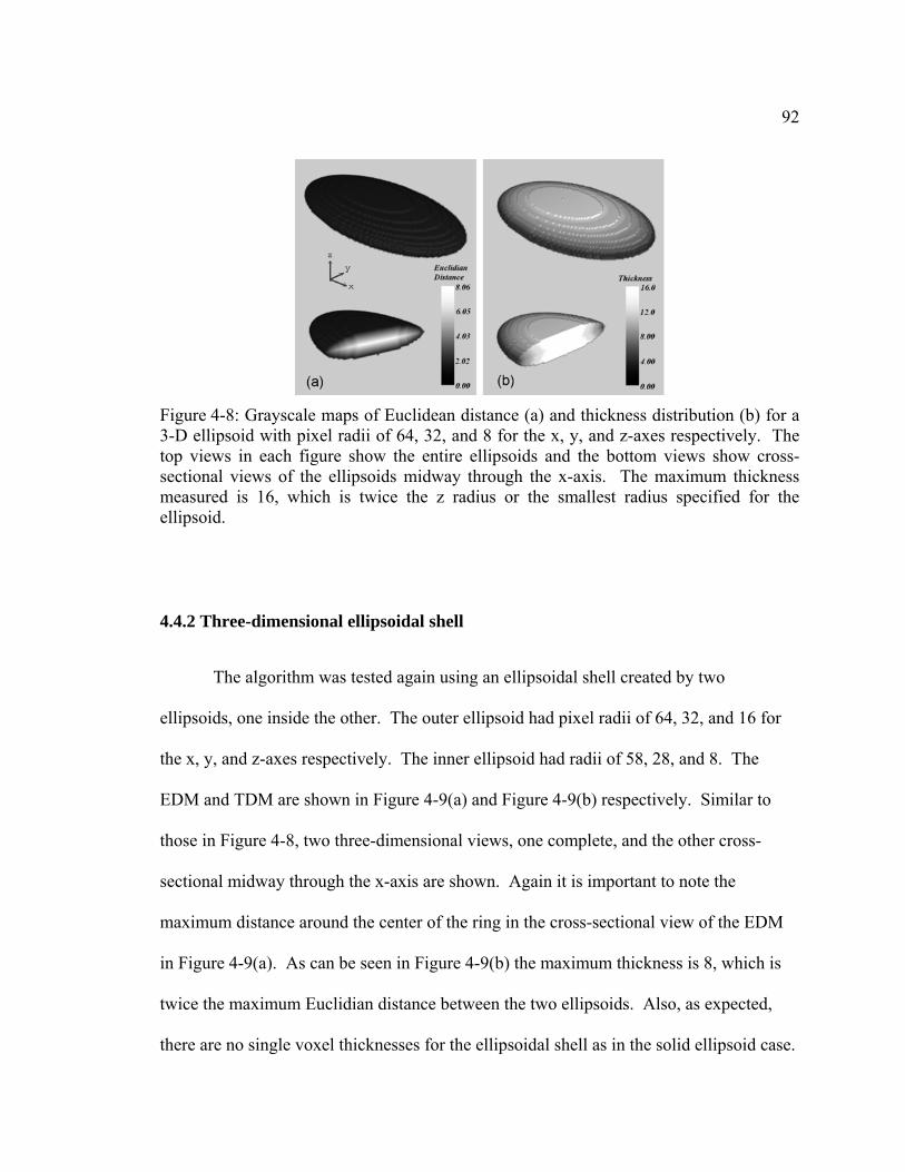
92

4-8: Grayscale mapFigure s of Euclidean distance (a) and thickness distribution (b) for a

The top vie ids and the bottom views show cross-

s measur the ellipsoi

3-D ellipsoid with pixel radii of 64, 32, and 8 for the x, y, and z-axes respectively. ws in each figure show the entire ellipso

sectional views of the ellipsoids midway through the x-axis. The maximum thicknesed is 16, which is twice the z radius or the smallest radius specified for d.

4.4.2 T

6 for

EDM and TDM are shown in Figure 4-9(a) and Figure 4-9(b) respectively. Similar to

those in

section ote the

maxim ss-sectional view of the EDM

in Figu s

twice th

there ar soidal shell as in the solid ellipsoid case.

hree-dimensional ellipsoidal shell

The algorithm was tested again using an ellipsoidal shell created by two

ellipsoids, one inside the other. The outer ellipsoid had pixel radii of 64, 32, and 1

the x, y, and z-axes respectively. The inner ellipsoid had radii of 58, 28, and 8. The

Figure 4-8, two three-dimensional views, one complete, and the other cross-

al midway through the x-axis are shown. Again it is important to n

um distance around the center of the ring in the cro

re 4-9(a). As can be seen in Figure 4-9(b) the maximum thickness is 8, which i

e maximum Euclidian distance between the two ellipsoids. Also, as expected,

e no single voxel thicknesses for the ellip

93

Figure 4-9: Grayscale maps of Euclidean distance (a) and thickness distribution (b) for a 3-D ellipsoid shell. The outer ellipsoid has pixel radii of 64, 32, and 16 for the x, y, andz-axes respectively. The inner ellipsoid has pixel radii of 58, 28, and 8 for the x, y, and z-axes respectively. The top views in each figure show the entire ellipsoids and the bottom views show cross-sectional views of the ellipsoids midway through the x axis. Asexpected the maximum thickness measured is 8 (difference between z radii) and theminimum thickness is 4 (difference between y radii).

4.5 Results

This section demonstrates thickness maps for segmented human tissue regions in

the knee and brain in MRI. The knee image was acquired at the Pennsylvania State

University Hershey Medical Center. The MR brain data set and its manual segmentation

were provided by the Center for Morphometric Analysis at Massachusetts General

Hospital and are available at http://www.cma.mgh.harvard.edu/ibsr/. For each image the

average thickness for each segmented tissue region was computed. Average thickness is

easily computed from the TDM’s as follows:

Maxiitotal

fffff

ffspfspfsp

ffsp

MaxMax

i

total

MaxMax

ii

total

+⋅⋅⋅++==

⋅+⋅⋅⋅+⋅+⋅==

∑

∑=

21

21

1τ

= 211

4.1

http://www.cma.mgh.harvard.edu/ibsr/

94

Where is the average thickness, sp

the

τ is the voxel spacing, is the voxel frequency for

the thickness value, and is s f each normalized by the

thi ess value ess he

ma um voxel thickness (in units of numb alization

frequencies to diameter frequencies for each thickness value.

Figure 4-10 shows the TDM for a normal human patellar cartilage of a young

normal subject using sagittally acquired 0.313 mm x 0.313 mm x 1.00 mm MR T1-

weighted water selective fluid images acquired at the Pennsylvania State University

Hershey Medical Center. Prior to segmentation the image was resampled to 0.313 mm

isotropic voxel size using cubic interpolation. Segmentation of the patellar cartilage was

performed semi-automatically using ITK-SNAP [22], available at

http://www.itksnap.org/

if

if

er of voxels). The norm

thi

ckn

xim

totalf

Max

ummation o

. The summations above are carried out over 1 voxel thickn

thi

to t

converts the voxel

Also presented are SPM results of cortical thickness for a paired t-test of 53 MCI

subjects and corresponding age and gendered matched normal controls.

4.5.1 MRI human knee patellar cartilage thickness

. Segmentation using ITK-SNAP took approximately 30 minutes

(including manually editing of the final segmentation result) and the thickness

calculation, using the proposed method, lasted 3 minutes and 46 seconds on a Pentium 4

m running at 3.4 GHz. The average thickness was 3.01±1.38 mm, which

is in clo mm

HT Linux syste

se agreement with previously published measurements of 3.05 mm and 2.8

[16, 23].

http://www.itksnap.org/

95

Figure ge displays the sagittal view of the MR T -weighted water selective fluid scan of human

images on the right are 3-D volume renderings of the TDM and image mask for the

emoved to display the inner thicknessdistribution. Average thickness was 3.011 mm.

4-10: Human patellar cartilage TDM calculated from MR image. The left ima1

knee (0.313 mm isotropic voxel size) with an overlay of the patellar cartilage TDM. The

patellar cartilage. A section of the cartilage was r

4.5.2 MRI human brain cortical thickness

4-11 shows the TDM for the human brain cortex. To test the method on

the hum

r

research. Along with measurements obtained from the manually-guided data, FSL [24],

freely available at http://www.fmrib.ox.ac.uk/fsl/

Figure

an brain cortex, a single normal subject T1-weighted MR image with 1.0 mm x

1.0 mm x 1.5 mm voxel size was selected at random from 1 of 18 high resolution images

available as part of the Internet Brain Segmentation Repository (IBSR). The IBSR data

was chosen because the image data is accompanied with manually-guided and labeled

gray, white, and cerebrospinal fluid tissue segmentations and is freely available fo

, was used to automatically segment the

http://www.fmrib.ox.ac.uk/fsl/

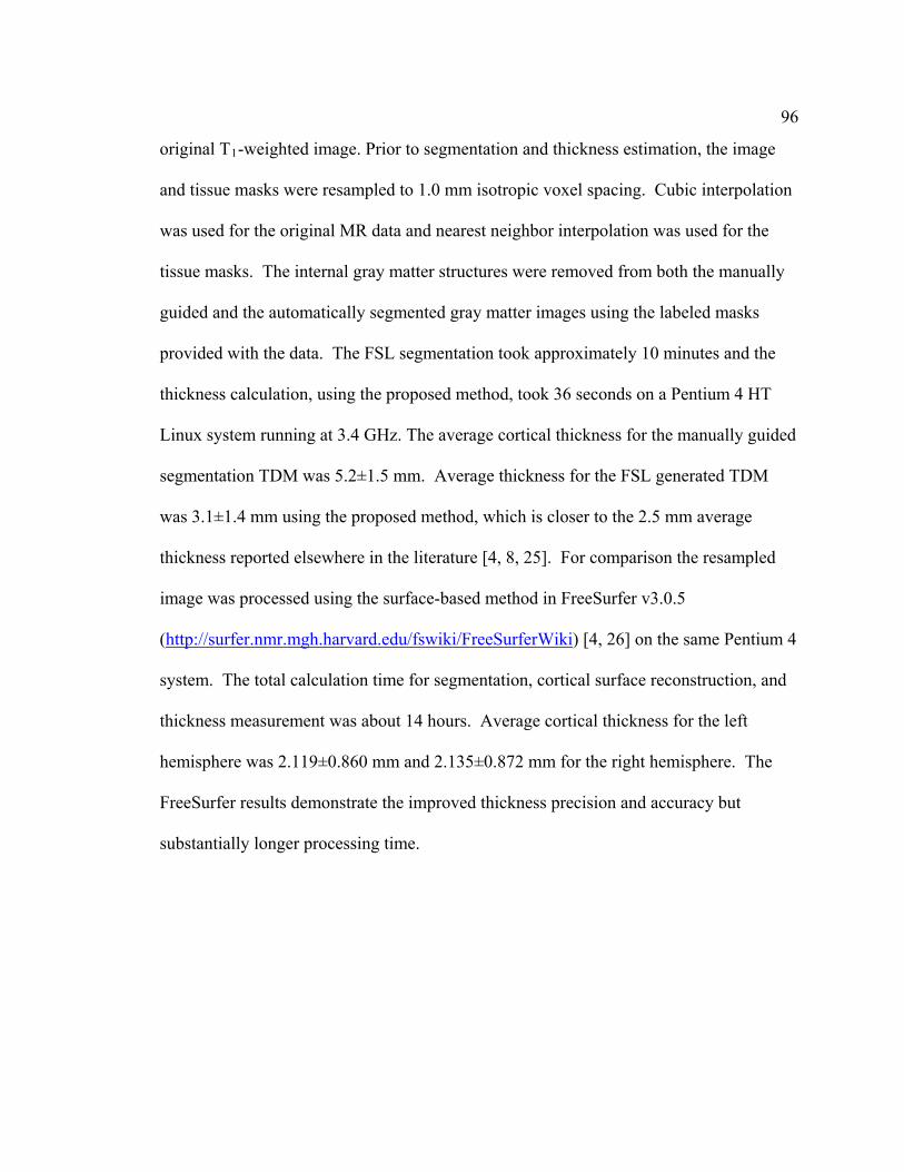
96

original T1-weighted image. Prior to segmentation and thickness estimation, the image

and tissue masks were resam

guided and the automatically segmented gray matter images using the labeled masks

was 3.1±1.4 mm using the proposed method, which is closer to the 2.5 mm average

(http://surfer.nm

pled to 1.0 mm isotropic voxel spacing. Cubic interpolation

was used for the original MR data and nearest neighbor interpolation was used for the

tissue masks. The internal gray matter structures were removed from both the manually

provided with the data. The FSL segmentation took approximately 10 minutes and the

thickness calculation, using the proposed method, took 36 seconds on a Pentium 4 HT

Linux system running at 3.4 GHz. The average cortical thickness for the manually guided

segmentation TDM was 5.2±1.5 mm. Average thickness for the FSL generated TDM

thickness reported elsewhere in the literature [4, 8, 25]. For comparison the resampled

image was processed using the surface-based method in FreeSurfer v3.0.5

r.mgh.harvard.edu/fswiki/FreeSurferWiki) [4, 26] on the same Pentium 4

system. The total calculation time for segmentation, cortical surface reconstruction, and

hemisphere was 2.119±0.860 mm and 2.135±0.872 mm for the right hemisphere. The

thickness measurement was about 14 hours. Average cortical thickness for the left

FreeSurfer results demonstrate the improved thickness precision and accuracy but

substantially longer processing time.

http://surfer.nmr.mgh.harvard.edu/fswiki/FreeSurferWiki

97

The 3-D view in Figure 4-11 shows the surface distribution of thickness in the

cortex using the proposed method. The sulci are largely hidden from view; therefore the

ral sections show up most prominently (yellowish-green). Sulcal

regions

thod. Higher

resolution MR images with improved CNR will alleviate this problem by improving the

segmentation results. Also, as can be seen in the 2-D sagittal view, poor segmentation of

Figure 4-11: Brain cortical TDM derived from the automatically-segmented image set. hree orthogonal projections of T1-weighted MR image of human head (left), the cortical

TDM overlay (middle), and 3-D volume renderings of the TDM and image mask (right) T

are shown. The average cortical thickness was 3.14 mm.

apparently thicker gy

are better visualized in the 2-D orthogonal projection views. The gyri appear to

be thicker in some areas due to the combination of poor gray and white matter

segmentation in those areas using FSL and undefined topology by this me

98

the medial temporal lobe region caused the thickness measurement to spike to the 12 mm

maximu

statistical analysis of brain cortical TDM, voxel-based SPM was performed using data

cess Series of Imaging Studies (OASIS) [27]. Fifty three MCI

subjects (average age 77.72 ± 7.14 years) and 53 age and gender matched NC subjects

was above 0. After matching by age, a two-

tailed t-tes

showed a significant difference between MCI and NC (P = 0.004). The TDM’s were

cerebellum and brainstem were removed from the final registered image. After

contrasts were examined, NC > MCI and MCI > NC. A 0.05 false discovery rate (FDR)

significant at this level.

m shown in the color bar.

4.5.3 MRI SPM paired t-test of MCI and normal controls

Figure 4-12 shows the SPM results of the paired t-test for normal controls (NC’s)

> MCI. In order to demonstrate the utility of the proposed method for group based

obtained from the Open Ac

(average age 77.74 ± 7.13 years, P = 0.99) were selected from the image dataset. All

subjects were matched by age within ± 3 years. Subjects were considered MCI if their

Clinical Dementia Rating (CDR) scale [28]

t of average years of education (2.68 ± 1.38 for MCI and 3.47 ± 1.41 for NC)

registered using the technique described in Chapter 3. As part of the processing, the

registration, the registered TDM’s were smoothed with an isotropic 5 mm FWHM

Gaussian kernel using SPM5. A paired t-test design was created within SPM5. Two

and 100 voxel extent was used to threshold the resultant t-maps. Only NC > MCI was

99

Areas of significant thinning were detected mainly in the temporal lobes, but

thinning was also detected in frontal areas and in the medial gyri. The most significant

thinnin e

d

poral, parahippocampal, lateral occipitotemporal, medial

front-orbital, lateral front-orbital, middle frontal, and inferior frontal gyri and the

rtex. All of the same regions, except the inferior temporal and lateral front-

orbital gyri, were also detected in this study. A different surface-based thickness study of

MCI [4, 31] identified brain co

g occurred in the right hippocampal formation, followed by the bilateral cingulat

region, left hippocampal formation, and bilateral thalamus. Hippocampal volume loss

and thinning is a hallmark of MCI, the precursor to AD [29]. A previous surface base

thickness study of MCI [5, 30] identified thinning in other regions as well, including the

inferior temporal, middle tem

entorhinal co

rtical thinning in the medial temporal cortex, inferior

temporal gyrus, temporal pole, inferior frontal sulcus, angular gyrus, superior frontal

gyrus, superior parietal lobule, supramarginal gyrus, and precuneus. The superior frontal

gyrus, superior parietal lobule, supramarginal gyrus, and precuneus also showed thinning

in MCI.

100

Figure 4-12: SPM t-maps for paired t-test of NC > MCI overlaid on the average

voxel extent of 100 was used to threshold the t-maps. (a) Right hippocampal formation.

smoothed cortical TDM of all of the subjects. A false discovery rate (FDR) of 0.05 and

(b) Bilateral cingulate region. (c) Left hippocampal formation. (d) Bilateral thalamus.

4.6 Discussion

An efficient method for the automatic estimation of thickness distribution of a 2-

D or 3-D structure of interest in segmented medical images has been presented in this

chapter. This method was validated using image objects with known thicknesses. The

101

utilization of the method for medical image analysis was demonstrated with estimations

of cortical thickness in human brain and cartilage thickness in human knee images.

Interestingly, the human cortex TDM’s from the manually guided segmentation, which is

generally considered to

be the “gold standard,” were on average thicker than the actual

average cortex measurement [25]. However, the TDM’s derived from the automatic

er to the previously reported average thickness values. These

results indicate that accurate estimates of brain cortical thickness using this method can

be achieved quickly and directly from th

in

and CNR. Nevertheless, discontinuities in the image object being measured will cause

igure 4-6(c) is an example of an image where the lack of a defined topology

causes the algorithm

ost

medical images discontinuities similar to Figure 4-6(c) are not common. Furthermore,

segmentation were clos

e segmented images produced with freely

available medical image segmentation tools. This is particularly advantageous for voxel-

based morphologic statistical studies of the brain involving multiple co-registered subject

images where the cumulative computation time can be prohibitively long. As

demonstrated in Section 4.5.3, the described method works well for these types of

studies. Furthermore, because the method is voxel-based, non-cortical brain structures

can be studied as well. For example, thinning of the thalamus in MCI was not reported

the surface-based studies, but was detected using this method.

In general, the accuracy of the thickness estimations using this approach depends

on the accuracy of the segmentation, which in turn depends on image resolution, SNR,

problems. F

described in this paper to behave in an undefined manner. Figure 4-

13 shows the thickness map output for Figure 4-6(c). Essentially, for this type of image

the topology must be defined in order to correctly measure thickness. However, for m

102

increasing the size of the search radius such that it encloses the entire object lessens this

problem. This also decreases the chance of marking small irregularities along the surface

of the object as having a thickness of one when in reality they should be marked with a

larger thickness value. The 3-D algorithm, as implemented for the knee and brain

images, uses this approach. Changing the search radius also changes the mapping

ickness and Euclidean distance. Table 4-2 shows the mapping that

works well for the 3-D implementation of the proposed method.

between voxel th

Figu 4-13: Thickness map of Figure 4-6(c) that illustrates problem where abrupt changein o ct boundary causes the algorithm to miss corner pixels. Increasing the size of the

ll cause the corner pixels to also be marke

re bje

search circle so that it encloses the object wi dwith ur. fo

103

Digital resolution is another factor that limits the accuracy of this method. The

mapping between pixel thickness and Euclidean distance shown in Table 4-1 and

-2 are required because ambiguities exist at low digital resolutions and betweeTable 4 n

ital

resolut

radii 2

three, f e

analog thicknesses. Also, defining the topology in this case does not help with correctly

Table 4

CE

ITS)

-2: Voxel thickness and corresponding Euclidean distance mappings.

VOXEL THICKNESS EUCLIDEAN DISTAN

(# OF VOXELS) (ARIBITRARY UN

1 1

2 1 to 2

3 1.42 to 2

4 2 to 5

5 2.25 to 3

6 3 to 10

7 + 2 ⋅ i, i =1,2,...,n − 2,n −1 3 + i to 10 + i

nnii ,1,...,2,1 ,28 −=⋅+ 3.17+ i to 4 + i

even and odd thicknesses described in Section 4.3.3.1. Figure 4-14 illustrates the dig

ion problem for digital circles with radii 1, 1.5, 2, and 2.5. The EDM for the

digital circles with radii 1 and 1.5 are exactly the same. The EDM for digital circles with

and 2.5 are slightly different, but still have the same squared Euclidean distance

value at their centers. In the analog domain the circles would have thicknesses of two,

our, and five respectively, but digitally it is difficult to exactly measure the tru

104

measuring the true analog thicknesses. The use of the pixel or voxel thickness to

an distance mapping allows the algorithm to identify and correct for ambiguitieEuclide s

The alg favors thicker pixel values in the case of ambiguities because it starts with

the thic

4.7 Re

005. [2] aton,

when possible, especially for the even and odd special case explained in Section 4.3.3.1.

orithm

kest value and ends with the thinnest value.

4-14: Illustration showing the ambiguities that exist in the EDM for low resolutioFigure n

digital focircles. Digital circles with radii 1 and 1.5 are exactly the same. The EDM rdigital circles with radii 2 and 2.5 both have five at their centers, even though their shapeare different. The proposed method described in Section 4.3 will favor thicker value

inner values in the case of ambiguities.

ss

over th

The C++ source code for the described method is listed in Appendix E.

ferences

P. M. Thompson, A.[1] D. Lee, R. A. Dutton, J. A. Geaga, K. M. Hayashi, M. A. Eckert, U. Bellugi, A. M. Galaburda, J. R. Korenberg, D. L. Mills, A. W. Toga,

d in and A. L. Reiss, "Abnormal cortical complexity and thickness profiles mappeWilliams Syndrome," The Journal of Neuroscience, vol. 25, pp. 4146-4158, 2F. Eckstein, M. Hudelmaier, W. Wirth, B. Kiefer, R. Jackson, J. Yu, C. B. Eand E. Schneider, "Double echo steady state magnetic resonance imaging of knee articular cartilage at 3 Tesla: A pilot study for the Osteoarthritis Initiative," Annals of the Rheumatic Diseases, vol. 65, pp. 433-441, 2006.

105

[3] M. Braten, A. Nordby, A. Terjesen, and I. Rossvoll, "Bone loss after locked intramedullary nailing. Computed tomography of the femur and tibia in 10 cases,"

[4] cerebral cortex

[5] A. C. Evans, "Automated 3-D extraction

[6] snick, D. L. Pham,

[7] d sing coupled-surfaces

[8]

[9] g tissue 03.

[10] e, vol. 40, pp. 1701-1710,

[11] ld, J. or

ication of cartilage thickness and volume changes using MRI: validation ng,

[12] MR images

medical

[13]

[14] apping," Computer Graphics and Image

[15] d picture with applications," Pattern

[16] mination of

Acta Orthopaedica Scandinavica, vol. 63, pp. 310-314, 1992. B. Fischl and A. M. Dale, "Measuring the thickness of the human from magnetic resonance images," Proceedings of the National Academy of Sciences of the United States of America, vol. 97, pp. 11050-11055, 2000. D. MacDonald, N. Kabani, D. Avis, andof inner and outer surfaces of cerebral cortex from MRI," NeuroImage, vol. 12, pp. 340-356, 2000. D. Tosun, M. E. Rettmann, X. Han, X. Tao, C. Xu, S. M. Reand J. L. Prince, "Cortical surface segmentation and mapping," NeuroImage, vol. 23, pp. S108-S118, 2004. X. Zeng, L. H. Staib, R. T. Schultz, and J. S. Duncan, "Segmentation anmeasurement of the cortex from 3-D MR images upropagation," IEEE Transactions on Medical Imaging, vol. 18, pp. 927-937, 1999. S. E. Jones, B. R. Buchbinder, and I. Aharon, "Three-dimensional mapping of cortical thickness using Laplace's Equation," Human Brain Mapping, vol. 11, pp. 12-32, 2000. A. J. Yezzi, Jr. and J. L. Prince, "An Eulerian PDE approach for computinthickness," IEEE Transactions on Medical Imaging, vol. 22, pp. 1332-1339, 20C. Hutton, E. De Vita, J. Ashburner, R. Deichmann, and R. Turner, "Voxel-basedcortical thickness measurements in MRI," NeuroImag2008. C. Kauffmann, P. Gravel, B. Godbout, A. Gravel, G. Beaudoin, J.-P. RaynauMartel-Pelletier, J.-P. Pelletier, and J. A. de Guise, "Computer-aided method fquantifstudy using a synthetic model," IEEE Transactions on Biomedical Engineerivol. 50, pp. 978-988, 2003. J. Tang, S. Millington, S. T. Acton, J. Crandall, and S. Hurwitz, "Surface extraction and thickness measurement of the articular cartilage fromusing directional gradient vector flow snakes," IEEE Transactions on BioEngineering, vol. 53, pp. 896-907, 2006. G. Borgefors, "Distance transformations in digital images," Computer Vision, Graphics, and Image Processing, vol. 34, pp. 344-371, 1986. P. E. Danielsson, "Euclidean distance mProcessing, vol. 14, pp. 227-248, 1980. T. Saito and J.-I. Toriwaki, "New algorithms for euclidean distance transformation of an n-dimensional digitizeRecognition, vol. 27, pp. 1551-1565, 1994. T. Stammberger, F. Eckstein, K.-H. Englmeier, and M. Reiser, "Deter3D cartilage thickness data from MR imaging: Computational method and reproducibility in the living," Magnetic Resonance in Medicine, vol. 41, pp. 529-536, 1999.

106

[17] P. K. Saha and F. W. Wehrli, "Measurement of trabecular bone thickness in the limited resolution regime of in vivo MRI by fuzzy distance transform," IEEE Transactions on Medical Imaging, vol. 23, pp. 53-62, 2004. T. Hildebrand and P. Ruegsegger, "A new method for the model-independ[18] ent

[19] iroutek, C. Lu, K. E. Muller, G.

. 85-

[20] , pp.

[21]

[22] G. :

ility," NeuroImage, vol. 31, pp. 1116-

[23] ccio, eas

litney,

[26] 9-194,

[27] . L.

ults,"

[28]

[29] orra, Z. Tu, L. G. Apostolova, A. E. Green, C. Avedissian, S. K. Madsen,

RI

doi:10.1016/j.neuroimage.2008.10.043.

assessment of thickness in three-dimensional images," Journal of Microscopy, vol. 185, pp. 67-75, 1997. S. M. Pizer, P. T. Fletcher, S. Joshi, A. Thall, J. Z. Chen, Y. Fridman, D. S. Fritsch, A. G. Gash, J. M. Glotzer, M. R. JTracton, P. Yushkevich, and E. L. Chaney, "Deformable M-Reps for 3D Medical Image Segmentation," International Journal of Computer Vision, vol. 55, pp106, 2003. P. A. Yushkevich, H. Zhang, and J. C. Gee, "Continuous Medial Representation for Anatomical Structures," IEEE Transactions on Medical Imaging, vol. 251547-1564, 2006. J. E. Bresenham, "Algorithm for Computer Control of a Digital Plotter," IBM Systems Journal, vol. 4, pp. 25-30, 1965. P. A. Yushkevich, J. Piven, H. C. Hazlett, R. G. Smith, S. Ho, J. C. Gee, andGerig, "User-guided 3D active contour segmentation of anatomical structuresSignificantly improved efficiency and reliab1128, 2006. Z. A. Cohen, D. M. McCarthy, S. D. Kwak, P. Legrand, F. Fogarasi, E. J. Ciaand G. A. Ateshian, "Knee cartilage topography, thickness, and contact arfrom MRI: In-vitro calibration and in-vivo measurements," Osteoarthritis and cartilage, vol. 7, pp. 95-109, 1999.

[24] S. M. Smith, M. Jenkinson, M. W. Woolrich, C. F. Beckmann, T. E. J. Behrens, H. Johansen-Berg, P. R. Bannister, M. De Luca, I. Drobnjak, and D. E. F"Advances in functional and structural MR image analysis and implementation asFSL," NeuroImage, vol. 23, pp. S208-S219, 2004.

[25] C. v. Economo and G. N. Koskinas, The Cytoarchitectonics of the Human Cerebral Cortex. London: Oxford University Press, 1929. A. M. Dale, B. Fischl, and M. I. Sereno, "Cortical surface-based analysis I: Segmentation and surface reconstruction," NeuroImage, vol. 9, pp. 171999. D. S. Marcus, T. H. Wang, J. Parker, J. G. Csernansky, J. C. Morris, and RBuckner, "Open Access Series of Imaging Studies (OASIS): Cross-sectional MRIData in Young, Middle Aged, Nondemented, and Demented Older AdJournal of Cognitive Neuroscience, vol. 19, pp. 1498-1507, 2007. J. C. Morris, "The Clinical Dementia Rating (CDR): Current version and scoring rules " Neurology, vol. 43, pp. 2412-2414, 1993. J. H. MN. Parikshak, A. W. Toga, C. R. Jack Jr, N. Schuff, M. W. Weiner, and P. M. Thompson, "Automated mapping of hippocampal atrophy in 1-year repeat Mdata from 490 subjects with Alzheimer's disease, mild cognitive impairment, andelderly controls," NeuroImage, vol. In Press, Corrected Proof, p.

107

2885-2893, 2006. eve, F.

, J. H. cal

c Amyloid-Positive Individuals," Cerebral Cortex, p.

[30] V. Singh, H. Chertkow, J. P. Lerch, A. C. Evans, A. E. Dorr, and N. J. Kabani, "Spatial patterns of cortical thinning in mild cognitive impairment and Alzheimer's disease," Brain, vol. 129, pp.

[31] B. C. Dickerson, A. Bakkour, D. H. Salat, E. Feczko, J. Pacheco, D. N. GrGrodstein, C. I. Wright, D. Blacker, H. D. Rosas, R. A. Sperling, A. AtriGrowdon, B. T. Hyman, J. C. Morris, B. Fischl, and R. L. Buckner, "The CortiSignature of Alzheimer's Disease: Regionally Specific Cortical Thinning Relatesto Symptom Severity in Very Mild to Mild AD Dementia and is Detectable in Asymptomatidoi:10.1093/cercor/bhn113, 2008.

Chapter 5

Amyotrophic Lateral Sclerosis (ALS): An Introduction

5.1 Brief history

During the 1800’s neurologists discovered that muscle weakness was due to eithe

s of the muscle or loss of neurons that support muscle. In the case of motor

r

disease

motor

neuron er motor

neuron

motor n ogists Charcot and Joffroy [1] named the

disease

commonly known as Lou Gehrig’s disease after the famous New York Yankee’s baseball

player

Since t ies: “classical” ALS (both UMN’s

and LM

primary ophy (PMA) (LMN symptoms only).

t

(CST) [2]. At post-mortem the brain appears normal except for atrophy in the primary

neuron disease, they noted that certain diseases were characterized by either upper

(UMN) (neurons of the central nervous system) deterioration or low

(LMN) (neurons of the spinal chord) deterioration. When both upper and lower

eurons degeneration were present, neurol

amyotrophic lateral sclerosis (ALS). In the United States, ALS is more

whose baseball career ended when he was diagnosed with the disease in 1939.

hen ALS has been classified into three categor

N’s symptoms); primary lateral sclerosis (PLS) (UMN symptoms only); and

muscular atr

5.2 Pathology

Pathology within the UMN typically begins within the primary motor and

premo or cortices leading to secondary degeneration of fibers along the corticospinal tract

109

motor c

.

layers I ically abnormal and

contain

structu Early reports established neurofilament

accumu

bad at

the

cranial . Gliosis is also present [3]. Loss of

the LM

se histopathologic studies have only been done on post mortem brains.

As a re

5.3 Etiology

Presently the exact causes of ALS are unknown. In 5-10% of reported cases, ALS

is linked to a mutation in superoxide dismutase 1 (SOD1). The number of mutations in

this form of “familial ALS” is 90 and counting [8, 9]. For the remaining cases, ALS is

thought to be a multifactorial disease involving genes and environmental agents (known

as “sporadic ALS”) [13, 14]. In either case, clinically they appear the same [10].

ortex (PMC). This atrophy is larger for patients who have had the disease longer

[3, 4] On the microscopic scale there is loss of Betz cells in the PMC and gliosis in

I and III [1, 4, 5]. The remaining motor neurons are histolog

various inclusion bodies and abnormalities of the neurofilament and microtubule

res. They also tend to be smaller [6].

lations in the motor neuron cell bodies as a sign of the disease [7-9]. Axonal

swelling of surviving motor tracks has also been observed and appears to be particularly

the internal capsules [7].

Pathology within the LMN is characterized by reduction of motor nuclei in

nerves and anterior horns of the spinal chord

N's leads to muscle weakness and wasting.

Overall, the

sult little is known about the in vivo pathology.

110

5.4 Diagnosis

Following AD and PD, ALS is t

Presently, no specific d LS remains a clinical

diagnosis. MRI is currently only used to rule out other possible neurological disorders.

gnosis varies considerably, but on average most ALS patients are

the middle ages. The disease develops rapidly giving the patient a life

nd

. This is referred to as “limb onset”. At other times, the

present with bulbar symptoms referred to as “bulbar onset”. The bulbar

is

using electromyography (EMG) which is crucial for clinical diagnosis. They

is

he third most common neurodegenerative disease.

iagnostic test exists for ALS. As a result, A

The age at dia

diagnosed in

expectancy of between two to five years after onset of symptoms. Typically, the first

symptom is muscle wasting and weakness in one of the limbs, including cramping a

fasciculations (muscle twitching)

patient will

symptoms are dysarthria (speech disorders) and dysphagia (difficulty swallowing). In

general, most limb onset patients develop bulbar symptoms as the disease progresses.

UMN symptoms include the Babinski sign (plantar response), Hoffmann’s sign

(upper limb equivalent of Babinski sign), spasticity, and hyperreflexia. Even so, there

no widely accepted objective marker for UMN involvement [11]. Early LMN symptoms

are shown

include diffuse fibrillation and fasciculation [12, 13].

In April of 1998, the World Federation of Neurology Research Group on Motor

Neuron Diseases held a consensus conference to develop revised criteria for the diagnos

of ALS [14]. During the conference, it was determined that for clinical studies the

diagnosis of ALS requires:

A - the presence of:

111

(A:1) evidence of LMN degeneration by clinical, electrophysiological or

B - the absence of:

(B:1) electrophysiological and pathological evidence of other disease processes

that might explain the signs of LMN and/or UMN degeneration, and

(B:2) neuroimaging evidence of other disease processes that might explain the

observed clinical and electrophysiological signs.

Furthermore, clinical diagnostic groups were devised as shown in Figure 5-1.

neuropathologic examination,

(A:2) evidence of UMN degeneration by clinical examination, and

(A:3) progressive spread of symptoms or signs within a region or to other

regions, as determined by history or examination,

together with

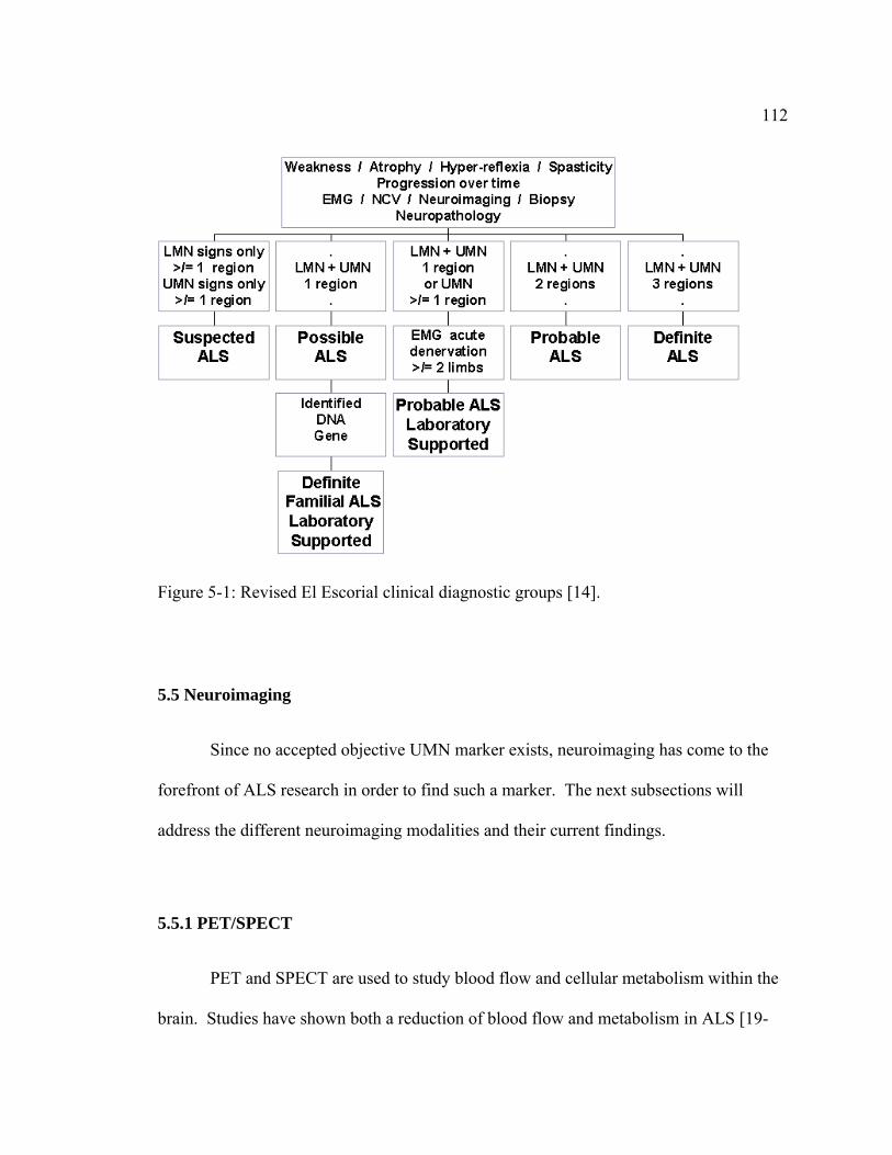
112

5.5 Neuroimaging

Since no accepted objective UMN marker exists, neuroimaging has come to the

forefront of ALS research in order to find such a marker. The next subsections will

address the different neuroimaging modalities and their current findings.

PET and SPECT are used to study blood flow and cellular metabolism within

brain. Studies have shown both a reduction of blood flow and metabolism in ALS [19-

5.5.1 PET/SPECT

the

Figure 5-1: Revised El Escorial clinical diagnostic groups [14].

113

22]. For ALS patients with signs of dementia, frontal regions show a similar reduction

[23, 24]. A PET activation study also showed a presence of cortical reorganization due to

motor n

ule

also been reported in the

frontotemporal WM, globus pallidus, thalamus, and subcortical frontal areas [23, 29].

T2-weighted hyperintensities in the brain are thought to be related to acute

demyelination, edema, or gliosis [18]. The causes of T2-weighted hypointensity in the

PMC are unknown, but may be explained by the presence of iron. A post-mortem study

of ALS found iron-laden astrocytes and macrophages in the PMC of some subjects [33].

e

euron loss [15]. However, these finding are not specific to ALS.

5.5.2 Conventional MRI

Standard T2-weighted, fluid attenuated inversion recovery (FLAIR), and proton

density weighted MRI have been used to examine ALS. In all three, hyperintensities

within the CST have been reported, in particular the posterior limb of the internal caps

(PLIC) [16-22].

Hyperintensities within the CST mainly at the PLIC [16, 23-32] and

hypointensities in the PMC [16, 23, 28, 32-37] have been observed in T2-weighted

imaging, but these observations are not 100% sensitive or specific to ALS [38].

Hyperintensities in PLIC are also seen in vitamin B12 deficiency [39], intracerebral

hemorrhage [40], and NC’s [18]. Although the majority of the studies focused on the

CST and motor cortex, T2-weighted hyperintensities have

A study using FLAIR suggested that this sequence was no more useful than th

T2-weighted sequence [17]. However, another study demonstrated that FLAIR image

114

intensities within the CST were more frequent in ALS patients than controls [20]. A

follow-up study showed that the image intensities increased significantly when compare

with the baseline scan [21].

5.5.3 MRS

Proton MRS (H-MRS) is a method to noninvasively measure the concentrations

of certain metabolites within the brain. A well established finding from using H-MRS is

a reduction of N-acetyl aspartate (NAA) in the PMC and brain stem [41-48]. The

decrease in NAA is thought to be due to neuronal degeneration and cell loss seen

histopathologically [5]. Abnor

d

malities correlated well with disease severity [41, 45]; but

did not correlate well with clinical scores of UMN degradation [45]. This finding might

be explained by the fact that clinical measures are insensitive to the severity of UMN

[45]. Reductions in NAA are seen outside of motor areas as well, like the postcentral

gyrus (PG), the superior parietal gyrus, and the posterior superior frontal gyrus [41]. This

is in agreement with the PET/SPECT findings discussed in Section 5.5.1. However,

reductions in NAA are not specific to ALS as they can also be found in NC’s [54, 58].

One study [47] used H-MRS to evaluate concentrations of glutamate (Glu), myo-

inositol (Ins), glutamine (Gln), and choline (Cho), in addition to NAA, within the PMC.

Glu and Gln were examined because studies have indicated that Glu excitotoxicity and

free radical-mediated oxidative injury play a role in the degeneration and death of motor

neurons in ALS [59-61]. The study determined that mean Cho and Ins were significantly

increased in ALS when compared with controls and that mean Glu and NAA were

115

decreased after adjusting for creatine covariance. These results all correlated with

severity of clinical UMN signs. Increased Cho might be due to either degradation of

membrane and mye h ipi 6 ccurs in demyelinating disorders,

or glial prolife tion ith ea in

a glial marker [49, 50]. As m io d i pathology studies have confirmed

the presence of gliosis.

5.5.4 DTI

DTI has been studied extensively in ALS [11, 19, 51-73]. The problem

studie is that re tt te et o d S s tion.

Small patient sampl ze pr m n particu ly ne R y elected

control regions in areas o e ST [53]. In whole-brain studies, two reported using

6 mm FWHM Gaussian kernel smo thi ], one reported a 10 mm FWHM

kernel size [68], another a 12 mm [74], and two d no h ern t [63,

64]. erms AL ub c , m ri e S e

Proba [11, , 54 , 69 , L e l s ected

[19, 53, 55, 57, 60, 62, 65 t rs s lecting ALS Probable only [74], ALS

Definite only [56, 67], A efinite and Suspected [58], familial ALS [71], or did not

report the El Escorial cla n a , ]. Therefore, it is difficult to draw

any c . In spite of the inconsistencies, a common

findin e CST when ALS is

comp

lin p osphol ds [ 2, 63], which o

ra w an incr se cell membrane precursors [48]. Ins is considered

ent ne n Section 5.2,

with these

s the is li le consis ncy in the m hod logies an AL patient elec

e si s are a oble too. I lar, on o OI stud s

utside th C

o ng size [55, 66

id t report t e k el size a all

In t of S s ject sele tion the vast ajo ty select d AL Definit and

ble 52 , 59 66, 68, , 72 73] or A S D finite, Probab e, and Su p

, 70]. O he reported e

LS D

ssificatio at ll [51, 63 64

oncrete conclusions from these studies

g is a reduction of FA in the CST and an increase of MD in th

ared with NC’s.

116

5.5.5 V

VBM results demonstrate GM atrophy not only in motor regions [68, 75-79], but

decrease in the CST [76, 81] and the subcortical frontal [76, 81, 82], temporal [82], and

dementia (FLTD) [75], showed that both groups have frontal lobe atrophy, but those with

tly more atrophied. Another VBM study that compared familial

ALS with sporadic ALS [79], demonstrated greater cortical atrophy in frontal areas for

s were compared to normal controls. All of these studies

suggest that the pattern of

The main focus of fMRI studies in ALS is on brain plasticity due to motor neuron

supplementary motor area (basil ganglia, brain stem, and cerebellum) [85, 91]. What

appears to be happening is that the loss of primary motor neurons leads to recruitment of

his strongly resembles activation patterns evoked in motor

learning. E

BM

also frontal [66-69, 71-73], temporal [68, 75, 78, 80], parietal [68], and occipital [68]

regions in ALS subjects when compared with NC’s. WM density was also shown to

occipital [76] regions. One study that compared ALS and ALS with frontal lobe-type

FLTD were significan

familial ALS when both group

cerebral atrophy varies considerably amongst ALS subjects.

5.5.6 fMRI

loss [83-90]. In general, there is an increase of neuronal activation within the

subcortical motor structures. T

ventually, fMRI studies in combination with other studies will be helpful in

piecing together the ALS puzzle.

117

5.6 References

[1] J. Charcot and A. Joffroy, "Deux cas d'astrophie muscolaire progressive avec lesions de la substance grise et des faisceaux antero-lateraux de la moelle

9. [2] R. A. Davidoff, "The pyramidal tract," Neurology, vol. 40, pp. 332-339, 1990. [3]

hic lateral sclerosis brains revisited," Annals of Neurology, vol. 24, p. .

[7] n,

n

d

, "From charcot to lou gehrig: deciphering th in als," Nature Reviews Neuroscience, vol. 2, pp.

[11] n

pp.

0.

epiniere," Arch Physiol Norm Pathol, vol. 2, pp. 744-760, 186

T. Lawyer and M. G. Netsky, "Amyotrophic lateral sclerosis: a clinicoanatomic study of fifty-three cases," Archives of Neurology and Psychiatry vol. 69, pp. 171-192, 1953.

[4] B. Brownell, D. R. Oppenheimer, and J. T. Hughes, "The central nervous system in motor neurone disease," Journal of Neurology, Neurosurgery, and Psychiatry,vol. 33, pp. 338-357, 1970.

[5] R. P. Hammer, U. Tomiyasu, and A. B. Scheibel, "Degeneration of the human Betz cell due to amyotrophic lateral sclerosis," Experimental Neurology, vol. 63, pp. 336-346, 1979.

[6] S. M. Chou and T. E. Huan, "Giant axonal spheroids in internal capsules of amyotrop168, 1988P. N. Leigh, A. Dodson, M. Swash, J. P. Brion, and B. H. Anderton, "Cytoskeletal Abnormalities in Motor Neuron Disease: An Immunocytochemical Study," Braivol. 112, pp. 521-535, 1989.

[8] M. Gaudette, M. Hirano, and T. Siddique, "Current status of SOD1 mutations ifamilial amyotrophic lateral sclerosis," Amyotrophic Lateral Sclerosis and Other Motor Neuron Disorders, vol. 1, pp. 83 - 89, 2000.

[9] P. M. Andersen, "Genetics of sporadic ALS," Amyotrophic Lateral Sclerosis anOther Motor Neuron Disorders, vol. 2, pp. S37 - S41, 2001.

[10] D. W. Cleveland and J. D. Rothsteinselective motor neuron dea806-819, 2001. Y.-H. Hong, K.-W. Lee, J.-J. Sung, K.-H. Chang, and I. C. Song, "Diffusiotensor MRI as a diagnostic tool of upper motor neuron involvement in amyotrophic lateral sclerosis," Journal of the Neurological Sciences, vol. 227, 73-78, 2004.

[12] A. Eisen and M. Swash, "Clinical neurophysiology of ALS," Clinical Neurophysiology, vol. 112, pp. 2190-2201, 2001.

[13] M. d. Carvalho, M. Scotto, A. Lopes, and M. Swash, "Clinical and neurophysiological evaluation of progression in amyotrophic lateral sclerosis," Muscle & Nerve, vol. 28, pp. 630-633, 2003.

[14] B. R. Brooks, R. G. Miller, M. Swash, and T. L. Munsat, "El Escorial revisited: Revised criteria for the diagnosis of amyotrophic lateral sclerosis," Amyotrophic Lateral Sclerosis and Other Motor Neuron Disorders, vol. 1, pp. 293-299, 200

118

[15] J. J. M. Kew, L. H. Goldstein, P. N. Leigh, S. Abrahams, N. Cosgrave, R. E.

abnormalities of cognitive function and cerebral activation in amyotrophic lateral

vol. 116, pp. 1399-1423, 1993.

lateral sclerosis: correlation of clinical and MR imaging findings [published

263-270, 1995.

Passingham, R. S. J. Frackowiak, and D. J. Brooks, "The relationship between

sclerosis: A neuropsychological and positron emission tomography study," Brain,

[16] G. Cheung, M. Gawel, P. Cooper, R. Farb, L. Ang, and M. Gawel, "Amyotrophic

erratum appears in Radiology 1995 Sep;196(3):800]," Radiology, vol. 194, pp.

[17] J. W. Thorpe, I. F. Moseley, C. H. Hawkes, D. G. MacManus, W. I. McDonald, and D. H. Miller, "Brain and spinal cord MRI in motor neuron disease," Journal of Neurology, Neurosurgery, and Psychiatry, vol. 61, pp. 314-317, 1996.

pinal tract 40, pp. 71-

75, 1998. [19]

amyotrophic lateral sclerosis: as assessed by serial computed gnetic resonance imaging," Journal of the Neurological

[24] hic

a,

[18] E. Hofmann, G. Ochs, A. Pelzl, and M. Warmuth-Metz, "The corticosin amyotrophic lateral sclerosis: An MRI study," Neuroradiology, vol.

C. M. Ellis, A. Simmons, D. K. Jones, J. Bland, J. M. Dawson, M. A. Horsfield, S. C. R. Williams, and P. N. Leigh, "Diffusion tensor MRI assesses corticospinal tract damage in ALS," Neurology, vol. 53, pp. 1051-, 1999.

[20] M. J. Hecht, F. Fellner, C. Fellner, M. J. Hilz, D. Heuss, and B. Neundorfer, "MRI-FLAIR images of the head show corticospinal tract alterations in ALS patients more frequently than T2-, T1- and proton-density-weighted images," Journal of the Neurological Sciences, vol. 186, pp. 37-44, 2001.

[21] M. J. Hecht, F. Fellner, C. Fellner, M. J. Hilz, B. Neundörfer, and D. Heuss, "Hyperintense and hypointense MRI signals of the precentral gyrus and corticospinal tract in ALS: A follow-up examination including FLAIR images," Journal of the Neurological Sciences, vol. 199, pp. 59-65, 2002.

[22] L. Zhang, A. M. Uluğ, R. D. Zimmerman, M. T. Lin, M. Rubin, and M. F. Beal, "The diagnostic utility of FLAIR imaging in clinically verified amyotrophic lateral sclerosis," Journal of Magnetic Resonance Imaging, vol. 17, pp. 521-527, 2003.

[23] S. Kato, H. Hayahi, and A. Yagishita, "Involvement of the frontotemporal lobe and limbic system intomography and maSciences, vol. 116, pp. 52-58, 1993. Y. Miaux, N. Martin-Duverneuil, C. Cognard, A. Weill, and J. Chiras, "Areas of high signal intensity in the posterior limbs of the internal capsules in amyotroplateral sclerosis: normal or pathologic MR finding?," Radiology, vol. 191, pp. 870b-871, 1994.

[25] A. Yagishita, I. Nakano, M. Oda, and A. Hirano, "Location of the corticospinal tract in the internal capsule at MR imaging," Radiology, vol. 191, pp. 455-460, 1994.

[26] S.-i. Terao, G. Sobue, T. Yasuda, T. Kachi, M. Takahashi, and T. Mitsum"Magnetic resonance imaging of the corticospinal tracts in amyotrophic lateral sclerosis," Journal of the Neurological Sciences, vol. 133, pp. 66-72, 1995.

119

[27] K. Abe, H. Fujimura, Y. Kobayashi, N. Fujita, and T. Yanagihara, "Degeneration

premortem and postmortem magnetic resonance imaging study," Journal of

[28] M. Waragai, "MRI and clinical features in amyotrophic lateral scle

of the pyramidal tracts in patients with amyotrophic lateral sclerosis. A

Neuroimaging, vol. 7, pp. 208-212, 1997. rosis,"

Neuroradiology, vol. 39, pp. 847-851, 1997. [29] E. Andreadou, P. Sgouropoulos, P. Varelas, A. Gouliamos, and C. Papageorgiou,

"Subcortical frontal lesions on MRI in patients with motor neurone disease,"

e, and L. P. Rowland, "Motor Neuron Diseases: Comparison of Single-Voxel Proton MR Spectroscopy

l Sciences, vol. 148,

[35] A. H. Karantanas, "Amyotrophic lateral sclerosis: unilateral T2-shortening on MRI," Computerized Medical Imaging and Graphics, vol. 22, pp. 353-355, 1998.

[36] H. Miwa, Y. Kajimoto, I. Nakanishi, S. Morita, J. Komoto, T. Kihira, and T. o, "T2-low signal intensity in the cortex in multiple system atrophy,"

Journal of the Neurological Sciences, vol. 211, pp. 85-88, 2003. [37] M. Hecht, C. Fellner, A. Schmid, B. Neundörfer, and F. Fellner, "Cortical T2

iron deposits,"

[38] Y. Iwasaki, K. Ikeda, Y. Ichikawa, O. Igarashi, and M. Kinoshita, "MRI in ALS

[39] ia:

pontine and thalamic myelinolysis in a normonatremic alcoholic," Clinical Radiology, vol. 47, pp. 137-138, 1993.

[41] E. P. Pioro, J. P. Antel, N. R. Cashman, and D. L. Arnold, "Detection of cortical neuron loss in motor neuron disease by proton magnetic resonance spectroscopic imaging in vivo," Neurology, vol. 44, pp. 1933-1938, 1994.

Neuroradiology, vol. V40, pp. 298-302, 1998. [30] S. Chan, D. C. Shungu, A. Douglas-Akinwande, D. J. Lang

of the Motor Cortex with MR Imaging of the Brain," Radiology, vol. 212, pp.763-769, 1999.

[31] P. Peretti-Viton, J. P. Azulay, S. Trefouret, H. Brunel, C. Daniel, J. M. Viton, A. Flori, B. Salazard, J. Pouget, G. Serratrice, and G. Salamon, "MRI of the intracranial corticospinal tracts in amyotrophic and primary lateral sclerosis," Neuroradiology, vol. 41, pp. 744-749, 1999.

[32] M. Basak, M. Erturk, B. Oflazoglu, A. Ozel, G. B. Yildiz, and H. Forta, "Magnetic resonance imaging in amyotrophic lateral sclerosis," Acta Neurologica Scandinavica, vol. 105, pp. 395-399, 2002.

[33] H. Oba, T. Araki, K. Ohtomo, S. Monzawa, G. Uchiyama, K. Koizumi, Y. Nogata, K. Kachi, Z. Shiozawa, and M. Kobayashi, "Amyotrophic lateral sclerosis: T2 shortening in motor cortex at MR imaging," Radiology, vol. 189, pp. 843-846, 1993.

[34] M. Waragai, Y. Takaya, and M. Hayashi, "Serial MRI and SPECT in amyotrophic lateral sclerosis: A case report," Journal of the Neurologicapp. 117-120, 1997.

Kond

signal shortening in amyotrophic lateral sclerosis is not due toNeuroradiology, vol. 47, pp. 805-808, 2005.

patients," Acta Neurologica Scandinavica, vol. 107, pp. 426-426, 2003. J. R. Berger and R. Quencer, "Reversible myelopathy with pernicious anemClinical/MR correlation," Neurology, vol. 41, pp. 947-948, 1991.

[40] M. Mascalchi, M. Cincotta, and M. Piazzini, "Case report: MRI demonstration of

120

[42] A. P. Jones, W. J. Gunawardena, C. M. A. Coutinho, J. A. Gatt, I. C. Shaw, and J. D. Mitchell, "Preliminary results of proton magnetic resonance spectroscopy in

Journal of the

f brainstem neuronal loss in amyotrophic lateral sclerosis with in vivo proton

Neurology, vol. 50, pp. 72-77, 1998. [45]

Neurology, A.

Younis, R. C. Duncan, and R. M. Quencer, "MR Imaging and Localized Proton

ents," Archives of

[49] A. Brand, C. Richter-Landsberg, and D. Leibfritz, "Multinuclear NMR Studies on the Energy Metabolism of Glial and Neuronal Cells," Developmental Neuroscience, vol. 15, pp. 289-298, 1993.

[50] J. Frahm and F. Hanefeld, "Localized Proton Magnetic Resonance Spectroscopy of Cerebral Metabolites," Neuropediatrics, vol. 27, pp. 64-69, 1996.

[51] S. Jacob, J. Finsterbusch, J. H. Weishaupt, D. Khorram-Sefat, J. Frahm, and H. Ehrenreich, "Diffusion tensor imaging for long-term follow-up of corticospinal tract degeneration in amyotrophic lateral sclerosis," Neuroradiology, vol. 45, pp. 598-600, 2003.

[52] A. T. Toosy, D. J. Werring, R. W. Orrell, R. S. Howard, M. D. King, G. J. Barker, D. H. Miller, and A. J. Thompson, "Diffusion tensor imaging detects corticospinal tract involvement at multiple levels in amyotrophic lateral sclerosis," Journal of Neurology, Neurosurgery, and Psychiatry, vol. 74, pp. 1250-1257, 2003.

[53] J. M. Graham, N. Papadakis, J. Evans, E. Widjaja, C. A. J. Romanowski, M. N. J. Paley, L. I. Wallis, I. D. Wilkinson, P. J. Shaw, and P. D. Griffiths, "Diffusion tensor imaging for the assessment of upper motor neuron integrity in ALS," Neurology, vol. 63, pp. 2111-2119, 2004.

[54] M. Karlsborg, S. Rosenbaum, M. R. Wiegell, H. Simonsen, H. B. W. Larsson, L. M. Werdelin, and O. Gredal, "Corticospinal tract degeneration and possible

motor neurone disease (amyotrophic lateral sclerosis)," Neurological Sciences, vol. 129, pp. 85-89, 1995.

[43] O. Gredal, S. Rosenbaum, S. Topp, M. Karlsborg, P. Strange, and L. Werdelin, "Quantification of brain metabolites in amyotrophic lateral sclerosis by localized proton magnetic resonance spectroscopy," Neurology, vol. 48, pp. 878-881, 1997.

[44] V. A. Cwik, C. C. Hanstock, P. S. Allen, and W. R. Wayne Martin, "Estimation o

magnetic resonance spectroscopy," C. Ellis, A. Simmons, C. Andrews, J. Dawson, S. Williams, and P. Leigh, "A proton magnetic resonance spectroscopic study in ALS: correlation with clinical findings," vol. 51, pp. 1104-1109, 1998.

[46] J. Suhy, R. G. Miller, R. Rule, N. Schuff, J. Licht, V. Dronsky, D. Gelinas, A. Maudsley, and M. W. Weiner, "Early detection and longitudinal changes in amyotrophic lateral sclerosis by 1H MRSI," Neurology, vol. 58, pp. 773-779, 2002.

[47] B. C. Bowen, P. M. Pattany, W. G. Bradley, J. B. Murdoch, F. Rotta, A. A.

Spectroscopy of the Precentral Gyrus in Amyotrophic Lateral Sclerosis," American Journal of Neuroradiology, vol. 21, pp. 647-658, 2000.

[48] W. Block, J. Karitzky, F. Traber, C. Pohl, E. Keller, R. R. Mundegar, R. Lamerichs, H. Rink, F. Ries, H. H. Schild, and F. Jerusalem, "Proton Magnetic Resonance Spectroscopy of the Primary Motor Cortex in Patients With Motor Neuron Disease: Subgroup Analysis and Follow-up MeasuremNeurology, vol. 55, pp. 931-936, 1998.

121

pathogenesis in ALS evaluated by MR diffusion tensor imaging," Amyotrophic Lateral Sclerosis and Other Motor Neuron Disorders, vol. 5, pp. 136-140, 2004.

[55] M. Sach, G. Winkler, V. Glauche, J. Liepert, B. Heimbach, M. A. Koch, C. Buchel, and C. Weiller, "Diffusion tensor MRI of early upper motor neuron involvement in amyotrophic lateral sclerosis," Brain, vol. 127, pp. 340-350, 2004.

[56] H. Yin, C. C. T. Lim, L. Ma, Y. Gao, Y. Cai, D. Li, Y. Liang, and X. Guo, "Combined MR spectroscopic imaging and diffusion tensor MRI visualizes corticospinal tract degeneration in amyotrophic lateral sclerosis," Journal of Neurology, vol. 251, pp. 1249-1254, 2004.

[57] S. Aoki, N. K. Iwata, Y. Masutani, M. Yoshida, O. Abe, Y. Ugawa, T. Masumoto, H. Mori, N. Hayashi, H. Kabasawa, S. Kwak, S. Takahashi, S. Tsuji, and K. Ohtomo, "Quantitative Evaluation of the Pyramidal Tract Segmented by Diffusion Tensor Tractography: Feasibility Study in Patients with Amyotrophic Lateral Sclerosis," Radiation Medicine, vol. 23, pp. 195-199, 2005.

[58] M. Cosottini, M. Giannelli, G. Siciliano, G. Lazzarotti, M. C. Michelassi, A. Del Corona, C. Bartolozzi, and L. Murri, "Diffusion-Tensor MR Imaging of Corticospinal Tract in Amyotrophic Lateral Sclerosis and Progressive Muscular Atrophy," Radiology, vol. 237, pp. 258-264, 2005.

[59] O. Ciccarelli, T. E. Behrens, D. R. Altmann, R. W. Orrell, R. S. Howard, H. Johansen-Berg, D. H. Miller, P. M. Matthews, and A. J. Thompson, "Probabilistic diffusion tractography: a potential tool to assess the rate of disease progression in amyotrophic lateral sclerosis," Brain, vol. 129, pp. 1859-1871, 2006.

[60] S. Wang, H. Poptani, M. Bilello, X. Wu, J. H. Woo, L. B. Elman, L. F. McCluskey, J. Krejza, and E. R. Melhem, "Diffusion Tensor Imaging in Amyotrophic Lateral Sclerosis: Volumetric Analysis of the Corticospinal Tract," American Journal of Neuroradiology, vol. 27, pp. 1234-1238, 2006.

[61] S. Wang, H. Poptani, J. H. Woo, L. M. Desiderio, L. B. Elman, L. F. McCluskey, J. Krejza, and E. R. Melhem, "Amyotrophic Lateral Sclerosis: Diffusion-Tensor and Chemical Shift MR Imaging at 3.0 T," Radiology, vol. 239, pp. 831-838, 2006.

[62] C. R. V. Blain, V. C. Williams, C. Johnston, B. R. Stanton, J. Ganesalingam, J. M. Jarosz, D. K. Jones, G. J. Barker, S. C. R. Williams, N. P. Leigh, and A.

A. Woo, S. Wang, L. F. A. McCluskey, L. B. A. Elman, E. R. A. Melhem, and J. C. A. Gee, "High-Dimensional Spatial Normalization of Diffusion Tensor Images Improves the Detection of White Matter Differences: An Example Study Using Amyotrophic Lateral Sclerosis," IEEE Transactions on Medical Imaging, vol. 26, pp. 1585-1597, 2007.

[65] H. Mitsumoto, A. M. Ulug, S. L. Pullman, C. L. Gooch, S. Chan, M. X. Tang, X. Mao, A. P. Hays, A. G. Floyd, V. Battista, J. Montes, S. Hayes, S. Dashnaw, P.

Simmons, "A longitudinal study of diffusion tensor MRI in ALS," Amyotrophic Lateral Sclerosis and Other Motor Neuron Disorders, vol. 8, pp. 348 - 355, 2007.

[63] J. Grosskreutz, C. Keil, L. Emmerich, R. Dengler, and T. Peschel, "ALS upper motoneuron involvement in DTI and VBM: A longitudinal MRI study," Clinical Neurophysiology, vol. 118, p. e36, 2007.

[64] Z. Hui, B. B. Avants, P. A. Yushkevich, J. H.

122

Kaufmann, P. H. Gordon, J. Hirsch, B. Levin, L. P. Rowland, and D. C. Shungu, "Quantitative objective markers for upper and lower motor neuron dysfunction in

py Quantification in the Corticospinal Tract of Patients with Amyotrophic Lateral Sclerosis Using a Probabilistic Mixture Model,"

[68] L. Thivard, P.-F. Pradat, S. Lehericy, L. Lacomblez, D. Dormont, J. Chiras, H.

morphometry study in amyotrophic lateral sclerosis: relationships with motor 889-

892, 2007. , N. Mertens, S. Hofer, K.-D. Merboldt, J. Dietrich, J. Frahm, and H.

Ehrenreich, "Callosal dysfunction in amyotrophic lateral sclerosis correlates with diffusion tensor imaging of the central motor system," Neuromuscular Disorders, vol. 18, pp. 398-407, 2008.

[70] N. K. Iwata, S. Aoki, S. Okabe, N. Arai, Y. Terao, S. Kwak, O. Abe, I. Kanazawa, S. Tsuji, and Y. Ugawa, "Evaluation of corticospinal tracts in ALS with diffusion tensor MRI and brainstem stimulation," Neurology, vol. 70, pp. 528-532, 2008.

[71] M.-C. Ng, J. T. Ho, S.-L. Ho, R. Lee, G. Li, T.-S. Cheng, Y.-Q. Song, P. W.-L. Ho, G. C.-Y. Fong, W. Mak, K.-H. Chan, L. S.-W. Li, K. D.-K. Luk, Y. Hu, D. B. Ramsden, and L. L.-Y. Leong, "Abnormal diffusion tensor in nonsymptomatic familial amyotrophic lateral sclerosis with a causative superoxide dismutase 1 mutation," Journal of Magnetic Resonance Imaging, vol. 27, pp. 8-13, 2008.

[72] L. Roccatagliata, L. Bonzano, G. Mancardi, C. Canepa, and C. Caponnetto, "Detection of motor cortex thinning and corticospinal tract involvement by quantitative MRI in amyotrophic lateral sclerosis," Amyotrophic Lateral Sclerosis, 2008.

[73] F. Agosta, M. A. Rocca, P. Valsasina, S. Sala, D. Caputo, M. Perini, F. Salvi, A. Prelle, and M. Filippi, "A longitudinal diffusion tensor MRI study of the cervical cord and brain in amyotrophic lateral sclerosis patients," Journal of Neurology, Neurosurgery, and Psychiatry, vol. 80, pp. 53-55, 2009.

[74] O. Abe, H. Yamada, Y. Masutani, S. Aoki, A. Kunimatsu, H. Yamasue, R. Fukuda, K. Kasai, N. Hayashi, T. Masumoto, H. Mori, T. Soma, and K. Ohtomo, "Amyotrophic lateral sclerosis: diffusion tensor tractography and voxel-based analysis," NMR in Biomedicine, vol. 17, pp. 411-416, 2004.

[75] J. L. Chang, C. Lomen-Hoerth, J. Murphy, R. G. Henry, J. H. Kramer, B. L. Miller, and M. L. Gorno-Tempini, "A voxel-based morphometry study of patterns of brain atrophy in ALS and ALS/FTLD," Neurology, vol. 65, pp. 75-80, 2005.

ALS," Neurology, vol. 68, pp. 1402-1410, 2007. [66] C. A. Sage, R. R. Peeters, A. Görner, W. Robberecht, and S. Sunaert,

"Quantitative diffusion tensor imaging in amyotrophic lateral sclerosis," NeuroImage, vol. 34, pp. 486-499, 2007.

[67] S. K. Schimrigk, B. Bellenberg, M. Schluter, B. Stieltjes, R. Drescher, J. Rexilius, C. Lukas, H. K. Hahn, H. Przuntek, and O. Koster, "Diffusion Tensor Imaging-Based Fractional Anisotro

American Journal of Neuroradiology, vol. 28, pp. 724-730, 2007.

Benali, and V. Meininger, "Diffusion tensor imaging and voxel based

disability," Journal of Neurology, Neurosurgery, and Psychiatry, vol. 78, pp.

[69] C. Bartels

123

[76] J. Kassubek, A. Unrath, H. J. Huppertz, D. Lule, T. Ethofer, A. D. Sperfeld, and A. C. Ludolph, "Global brain atrophy and corticospinal tract alterations in ALS, as investigated by voxel-based morphometry of 3-D MRI," Amyotrophic Lateral Sclerosis and Other Motor Neuron Disorders, vol. 6, pp. 213-220, 2005.

[77] J. Grosskreutz, J. Kaufmann, J. Fradrich, R. Dengler, H.-J. Heinze, and T. Peschel, "Widespread sensorimotor and frontal cortical atrophy in Amyotrophic Lateral Sclerosis," BioMed Central Neurology, vol. 6, p. 17, 2006.

[78] F. Agosta, E. Pagani, M. A. Rocca, D. Caputo, M. Perini, F. Salvi, A. Prelle, and M. Filippi, "Voxel-based morphometry study of brain volumetry and diffusivity in amyotrophic lateral sclerosis patients with mild disability," Human Brain Mapping, vol. 28, pp. 1430-1438, 2007.

[79] M. R. Turner, A. Hammers, J. Allsop, A. Al-chalabi, C. E. Shaw, D. J. Brooks, P. N. Leigh, and P. M. Andersen, "Volumetric cortical loss in sporadic and familial amyotrophic lateral sclerosis," Amyotrophic Lateral Sclerosis, vol. 8, pp. 343 - 347, 2007.

[80] D. M. Mezzapesa, A. Ceccarelli, F. Dicuonzo, A. Carella, M. F. De Caro, M. Lopez, V. Samarelli, P. Livrea, and I. L. Simone, "Whole-Brain and Regional Brain Atrophy in Amyotrophic Lateral Sclerosis," American Journal of Neuroradiology, vol. 28, pp. 255-259, 2007.

[81] C. M. Ellis, J. Suckling, E. Amaro, Jr., E. T. Bullmore, A. Simmons, S. C. R. Williams, and P. N. Leigh, "Volumetric analysis reveals corticospinal tract degeneration and extramotor involvement in ALS," Neurology, vol. 57, pp. 1571-1578, 2001.

[82] S. Abrahams, L. H. Goldstein, J. Suckling, V. Ng, A. Simmons, X. Chitnis, L. Atkins, S. C. R. Williams, and P. N. Leigh, "Frontotemporal white matter changes in amyotrophic lateral sclerosis," Journal of Neurology, vol. 252, pp. 321-331, 2005.

[83] S. Abrahams, L. H. Goldstein, A. Simmons, M. Brammer, S. C. R. Williams, V. Giampietro, and P. N. Leigh, "Word retrieval in amyotrophic lateral sclerosis: a functional magnetic resonance imaging study," Brain, vol. 127, pp. 1507-1517, 2004.

[84] M. A. Schoenfeld, C. Tempelmann, C. Gaul, G. R. Kühnel, E. Düzel, J.-M. Hopf,

Experimental Brain Research, vol. 172, pp. 361-369, 2006. [86]

Migliaccio, F. L. Conforti, R. Morrone, and A. Quattrone, "Subcortical motor

Bulletin, vol. 69, pp. 489-494, 2006.

Birbaumer, "Brain responses to emotional stimuli in patients with amyotrophic lateral sclerosis (ALS)," Journal of Neurology, vol. 254, pp. 519-527, 2007.

H. Feistner, S. Zierz, H.-J. Heinze, and S. Vielhaber, "Functional motor compensation in amyotrophic lateral sclerosis," Journal of Neurology, vol. 252, pp. 944-952, 2005.

[85] C. Konrad, A. Jansen, H. Henningsen, J. Sommer, P. Turski, B. Brooks, and S. Knecht, "Subcortical reorganization in amyotrophic lateral sclerosis,"

A. Tessitore, F. Esposito, M. R. Monsurro, S. Graziano, D. Panza, A. Russo, R.

plasticity in patients with sporadic ALS: An fMRI study," Brain Research

[87] D. Lulé, V. Diekmann, S. Anders, J. Kassubek, A. Kübler, A. Ludolph, and N.

124

E. Kraft, "Cortical Plasticity in Amyotrophic Lateral Sclerosis: Motor Imagery

vol. 21, pp. 518-526, 2007.

[89] Simmons, "Altered cortical activation during a motor task in ALS," Journal of

[90] B. R. Stanton, V. C. Williams, P. N. Leigh, S. C. R. Williams, C. R. V. Blain, V.

reduced in Amyotrophic Lateral Sclerosis," Brain Research, vol. 1172, pp. 145-

[91] B. R. Brooks, K. Bushara, A. Khan, J. Hershberger, J. O. Wheat, D. Belden, and H. Henningsen, "Functional magnetic resonance imaging (fMRI) clinical studies in ALS - paradigms, problems and promises," Amyotrophic Lateral Sclerosis and

[88] D. Lulé, V. Diekmann, J. Kassubek, A. Kurt, N. Birbaumer, A. C. Ludolph, and

and Function," Neurorehabilitation and Neural Repair,

B. Stanton, V. Williams, P. Leigh, S. Williams, C. Blain, J. Jarosz, and A.

Neurology, vol. 254, pp. 1260-1267, 2007.

P. Giampietro, and A. Simmons, "Cortical activation during motor imagery is

151, 2007.

Other Motor Neuron Disorders, vol. 1, pp. S23-S32, 2000.

Chapter 6

ALS Brain Cortical Thickness Analysis

6.1 Abstract

Objective:

Measure brain cortical thickness in ALS using MRI cross-sectionally and longitudinally

to examine the relationship between cortical thickness and ALS clinical expression

regionally and within the PMC.

Methods:

High-resolution T1-weighted MRI was acquired from 21 age and gender-matched NC’s

and 14 ALS at baseline, 8 at 6 months, 6 at 12 months, and 4 at 18 months. STAMPS

was used to register and label cortical TDM’s. SPM5 was used for statistics analysis of

smoothed and registered TDM’s. R was used for ROI statistics within the PMC and

PCG. Excel was used for multiple regression of thickness with cognitive exams and age.

Results:

C was significantly

thinner

ckness

correlated significantly with cognitive exams in the left inferior temporal gyrus and right

inferior occipital gyrus.

Voxel-based statistical analysis of TDM’s did not reveal significant clusters cross-

sectionally or longitudinally. Using the ROI approach, the right PM

for the ALS limb only and ALS probable groups. Longitudinally, the left PMC

thickness correlated with time, disease duration, and severity. Cortical thi

126

Conclusions:

cortical thickness has sensitivity for evaluation of disease severity. Neurodegeneration in

ALS appears widespread into inferior and temporal gyri that correlates cognitive decline

due to disease.

Cortical thinning in ALS is slight. Gray matter thinning is found in ALS, which reflects

neurodegeneration associated with the disease. The developed method for estimating

127

6.2 Introduction

As discussed in Chapter 5, currently ALS remains a clinical diagnosis. Often, an

exhaustive evaluation is undertaken to rule out other diseases. Thus, there is a pressing

need for development of clinically useful and readily available imaging biomarkers of

ALS. Such biomarkers could potentially increase diagnostic accuracy, reduce

unnecessary testing and surgery, and permit longitudinal follow-up of disease progression

in clinical trials. Of all the qMRI methods examined to date, brain cortical thickness is

the least studied in ALS. Only two cortical thickness studies in ALS have been reported

[1, 2]. In one study, the ALS patients chosen were classified with PLS [1], the UMN

only variant of ALS (see Chapter 5). Using manual tools, they calculated thickness

within the PMC and the primary sensory cortex (PSC) at various locations and then

compared the average thicknesses with those derived from control subjects. They

demonstrated that the average bilateral 2.32 ± 0.21 mm PMC thickness for PLS subjects

was significantly thinner than the average 2.79 ± 0.18 mm thickness for normal controls

eesurfer (Chapter 2,

Section ) to measure and compare cortical thickness automatically in ALS Definite

and Probable subjects and normal controls [2]. They also demonstrated that the 1.97 ±

0.33 mm average bilateral PMC thickness in ALS was significantly thinner than the

average 2.14 ± 0.14 mm thickness for normal controls (P < 0.05). Also, no significant

(P = 0.0008). Thickness was not significantly decreased in the PSC or the posterior and

anterior banks of the precentral sulcus. The other study used Fr

2.4.2

128

thinning was detected in the postcentral and lateral occipital cortices and no correlation

was found between thickne

aver imaging of freshly excised ALS brains within the Penn State Center

for Nuclear Magnetic Resonance Research (CNMRR), showed a conspicuous loss of T1-

contrast between GM and WM within the PMC [3, 4]. Furthermore,

prelim nd 8 age-m

estimation techniqu cribed in er 4 dem ated thin 7 of th LS

subjects [5, 6]. It was thought that the thinning seen within the PMC was due to the loss

of T con ast between GM and WM and so the term

thin s coined. At this point the causes o T hted co

between GM and WM in the PMC are uncertain. However, it was hypothesized that

t

correlates with ALS clinical scores of severity (ALS Functional Rating Score) and/or

isease duration. The work presented in this chapter summarizes the methods and results

for the cross-sectional and longitudinal analysis of thickness in ALS using the thickness

estimation technique described in detail in Chapter 4.

6.3 Materials and methods

ss and clinical scores.

Early cad

weighted

inary qualitative analysis of 9 ALS a atched controls using the thickness

e des Chapt onstr ning in e 9 A

1-weighted tr “apparent cortical

ning” wa f the loss of 1-weig ntrast

hinning in the PMC was due to ALS disease progression and that thinning in the PMC

d

6.3.1 Subjects

ALS patients that met the revised El Escorial diagnostic criteria for definite,

probable, probable lab-supported, or suspected (Chapter 5, Section 5.4) were recruited

129

from the Penn State Milton S. Hershey Medical Center ALS Clinic. ALS suspected

subjects were included, because in most cases these subjects progress to ALS definite,

probable, or probable lab-supported through the course of the disease [1, 2]. Fourteen

ALS subjects (10 male and 4 female, average age 56.3 ± 13.3 years) were recruited at

baseline. Eight ALS subjects returned for a follow-up visit approximately 6 months

baseline, 6 subjects at approximately 12 months, and 4 subjects at approximately 18

months. For each image date, the ALS Functional Rating Score-Revised (ALSFRS-R)

and disease duration from onset of symptoms were recorded. Patients were clas

time of imaging by El Escorial criteria and by limb only, bulbar only, and generalized

(both limb and bulbar). Table

after

sified at

6-1 summarizes the demographic and disease information

for each ALS subject.

130

Table 6-1: ALS Patient demographic and disease information for baseline, 6 month, 1month, and 18 month visits.

2

Baseline 6 Months 12 Months 18 Months Subject # Sex Age Disease Disease Disease Disease Duration 41.1ALSFRS-R 21Class L

1 M 37.4

El Escorial PL

Withdrew from study.

Duration 58.0ALSFRS-R 26Class L

2 M 40.4

El Escorial S

Unable to lie flat due

to disease progression.

Duration 20.7 Duration 26.9 Duration 32.7 ALSFRS-R 32 ALSFRS-R 28 ALSFRS-R 20Class G Class G Class G

3 M 42.3

El Escorial D El Escorial D El Escorial D



Duration 24.6 Duration 29.8ALSFRS-R 19 ALSFRS-R 13Class G Class G

4 M 43.6

El Escorial D El Escorial D



Duration 19.5 Duration 24.7 Duration 31.0 Duration 35.6ALSFRS-R 43 ALSFRS-R 39 ALSFRS-R 36 ALSFRS-R 40Class G Class G Class G Class G

5 F 44.1

El Escorial PL El Escorial PL El Escorial PL El Escorial PLDuration 40.5 Duration 53.0 ALSFRS-R R35 ALSFRS- 36Class L Class L

6 F 55.0

El Escorial P

Missed appointment.

El Escorial P



Duration 46.5 Duration 52.2 Duration 58.2 Dur. 64.6ALSFRS-R 37 ALSFRS-R 34 ALS R RFRS- 33 ALSFRS- 32Class L Class L Class L Class L

7 M 56.5

El Escorial P El Escorial P El Escorial P El Escorial PDuration 15.1ALSFRS-R 43Class G

8 F 56.3

El Escorial P

Died.

Duration 50.7ALSFRS-R 40

9 F

Class G

60.9

El Escorial D



Duration 41.0 Duration 46.3 Duration 55.5 Duration 62.9ALSFRS-R R R R 2632 ALSFRS- 24 ALSFRS- 22 ALSFRS-Class G Class G Class G Class G

10 M 62.2

El Escorial S El Escorial S El Escorial S El Escorial SDuration 29.7 Duration 38.3 Duration 42.5 Duration 48.7ALSFRS-R 39 ALSFRS-R 37 ALSFRS-R 35 ALSFRS-R 33Class L Class L Class L Class L

11 M 65.6

El Escorial PL El Escorial PL El Escorial P El Escorial PDuration 76.6 Duration 81.4ALSFRS-R 30 ALSFRS-R 27Class L Class L

12 M 68.1

El Escorial S El Escorial S

Withdrew from study.

Duration 41.3ALSFRS-R 27

13 M 75.4 Died.

Class LEl Escorial PDuration 41.3 Duration 46.3ALSFRS-R 32 ALSFRS-R 20Class G Class G

14 M 79.8

El Escorial P El Escorial P

Died.

D

A

Cla

El

uration = disease duration from onset of symptoms in months.

LSFRS-R = ALS Functional Rating Score-Revised .

ss = disease classification based on limb (L), bulbar (B), and both limb and bulbar or generalized (G).

Escorial = El Escorial criteria is abbreviated as follows: D = clinical definite ALS, P = clinical probable ALS, PL = clinical probable A

laboratory supported, and S = clinical suspected ALS.

131

Fourteen age and gender matched normal control subjects (average age 56.0 ±

= 0.76) without neurological or neuromuscular diseases were also recruited fo

y. All participants w

13.0, P r

the stud ere provided written informed consent and approval for

human ge of

describ ubjects were included from a

previou otocol No.

6.3.2 M

over,

A, USA) using a body transmit coil and a 6 channel phase-array head receive coil. For

volumetric measurements, an axial whole-brain T1-weighted MDEFT (TE = 3.14 ms, TR

= 10.55 ms, TI = 680 ms, SENSE factor = 2, 20° flip angle, 1 mm isotropic voxel

resolution) image was acquired for each subject. The number of slices was adjusted to

cover the entire skull of each subject.

6.3.3 Image post-processing

Image post-processing was performed using STAMPS (Chapter 3) [7]. During

STAMPS processing the option for removing the brainstem and cerebellum was turned

on. Average thickness (Eq. 4.1) of each subject in the subject space was determined

research was obtained from the Institutional Review Board (Penn State Colle

Medicine IRB Protocol No. 20473). For the average thickness ANCOVA analysis

ed in Section 6.3.5, an additional 7 normal control s

s study on memory and aging (Penn State College of Medicine IRB Pr

19955).

R-Imaging protocol

Images were acquired on a 3.0 Tesla system (Intera, Philips Healthcare, And

M

132

automatically for each brain structure identified within the HAMMER supplied labeling

atlas using the TDM’s and the tool described in Chapter 3, Section 3.7.

6.3.4 Cross-sectional and longitudinal cortical thickness analysis

Voxel-based statistical analysis for thickness images was performed using SPM5.

ysis the images were smoothed with a 5 mm FWHM Gaussian kernel and an

ernel size was chosen based on the minimum size used in the validation of

,

lding the statistic maps with a p-value of 0.001 uncorrected. The minimum

e was set to 50 voxels.

full factorial designs grouped by baseline ALS, 6 months ALS, and 12

ith time, disease duration from onset of symptoms, and ALSFRS-R as

Prior to anal

explicit mask was generated from the average smoothed image of all of the subjects by

iteratively increasing a minimum threshold value such that the final mask only contained

GM. The k

RAVENS [8].

A paired t-test (14 conditions, 2 blocks, 16 total having 15 degrees of freedom

leaving 13 degrees of freedom from 28 images) was used to locate brain regions with

significant thinning between controls and baseline ALS. These regions were highlighted

by thresho

cluster siz

Four statistical longitudinal models were examined based on the available

longitudinal ALS image data. In all four models, the independence option was set to

“No”, to account for dependency in the repeated measures. First, a paired t-test (8

conditions, 2 blocks, 10 total having 9 degrees of freedom, leaving 7 degrees of freedom

from 16 images) between baseline and 6 months ALS was performed. The remaining

three models were

months ALS w

133

covariates. Only those subjects that were imaged on all three time points were included

in the three groups (3 conditions, 1 covariate, 4 total having 11 degrees of freedom from

15 images for each model). Statistically significant brain regions were highlighte

thresholding the statistic maps u

d by

sing a false discovery rate (FDR) of 0.05 and a minimum

cluster size of 50 voxels.

6.3.5 Cross-sectional and longitudinal primary motor thickness analysis

Average thickness of the right and left PMC and postcentral gyrus (PCG) in the

subject space were analyzed using the R statistical software package (http://www.r-

project.org/). Two ANCOVA models were used to compare ALS and controls. In one

model, the subjects were grouped by control, ALS limb only and ALS generalized (no

ALS bulbar patients were selected during the duration of the study). In the other model,

subjects were grouped by control and ALS El Escorial criteria. For both models age was

used as a covariate. No interactions were modeled. As mentioned in Section 6.3.1 an

additional 7 normal subjects were added to the group analysis for a total of 21 (average

age 57.5 ± 12.1, P = 0.79).

A linear mixed effects analysis with time from baseline as the random effect was

used to test correlation of average thickness for the right and left PMC and PCG with

time from baseline and ALS Functional Rating Score-Revised (ALSFRS-R). A similar

model was used with disease duration as the random effect to test correlation of average

thickness with disease duration from onset of symptoms. All ALS subjects that

completed at least two scans and grouped by limb and generalized were included in the

http://www.r-project.org/


134

analysis. Linear regression of average thickness for the right and left PMC and PCG with

age in years was performed on the control subjects and the average slope was used to

al ALS thickness values prior to statistical analysis.

te

rior

Based on the thresholding criteria specified in Section 6.3.4, no regions of

significant cortical thinning were identified cross-sectionally or longitudinally.

correct the longitudin

6.3.6 Regional average cortical thickness and cognitive exams

A subset of the subjects listed in Table 6-1 were administered the Penn Sta

Screen Exam of Frontal and Temporal Dysfunction Syndromes (PSSFTS), a refinement

of the recently published screen of frontal dysfunction [9]. Multiple regression analysis

of average thickness and age to cognitive exam scores was performed in Excel for select

brain regions that included the lateral orbital frontal gyrus, medial frontal gyrus, infe

frontal gyrus, PMC, superior temporal gyrus, medial temporal gyrus, inferior temporal

gyrus, superior occipital gyrus, superior parietal lobule, angular gyrus, middle occipital

gyrus, inferior occipital gyrus, and lateral occipitotemporal gyrus.

6.4 Results

6.4.1 Cross-sectional and longitudinal cortical thickness analysis

135

6.4.2 Cross-sectional and longitudinal primary motor cortex thickness analysis

For the left PMC ANCOVA analysis, no significant group effect was observed,

ively with age (P = 0.0003). Similarly, for the left PCG, no

significant group effect was observed, but thickness correlated negatively with age (P =

84) and the limb only

group (P = 0.0322) were significant for the ALS limb, bulbar, and generalized group

model. The ALS generalized group approached significance (P = 0.0792). Figure 6-1

shows the scatter plot of thickness as a function of age for this model. For the same brain

region e correlation (P = 0.0456) and

group effect existed for the ALS probable group (P = 0.0006). The ALS Definite group

.0893). Figure 6-2 shows the scatter plot of thickness as a

function of age for the El Escorial grouped model.

but thickness correlated negat

0.0258).

For the right PMC ANCOVA analysis, both age (P = 0.00

but grouped by El Escorial, a significant negative ag

approached significance (P = 0

136

Figure 6-1: Scatter plot of right primary motor cortex (PMC) thickness versus age for theANCOVA model grouped by Controls = C, ALS Limb only = L, and ALS Generalized(Limb and Bulbar) = G (defined in Table 6-1). The ALS Limb group was significant (P= 0.0322). The ALS Generalized approached significance (P = 0.079

2). The correlation

of thickness with age for each group is also plotted.

137

Figure 6-2: Scatter plot of right primary motor cortex (PMC) thickness versus age for thANCOVA model grouped by Controls = C and El Escorial classification. Table 6-1defines the El Escorial symbols used in the plot. The ALS Probable group wassignificant (P = 0.0006) 0.0893). The correlation of thickness with ag

e

and the ALS Definite group approached significance (P =e for the Control, ALS Probable, and ALS

Definite groups are also plotted.

For the right PCG ANCOVA model grouped by El Escorial, a significant group

effect was seen for the ALS Probable group (P = 0.0027). Significant age correlation

138

with thickness was not observed. Figure 6-3 shows the scatter plot of thickness as a

function of age.

Figure 6-3: Scatter plot of right postcentral gyrus (PCG) thickness versus age for tANCOVA model grouped by Controls = C and El Escorial classification. Table 6-defines the El Escorial symbols used in the plot. The ALS Probable group w

he1

assignificant (P = 0.0027). The correlation of thickness with age was not significant.

139

The correlation of the left PMC with age for the control group was significant (P

therefore no age correction was performed for these two gyri.

Longitudinally, the right PMC and PCG were not significant for any of the

models. In addition no significant longitudinal group effect existed for the PMC or the

PCG. The left PMC showed a significant negative correlation of age corrected thickness

with time (P = 0.0185) and disease duration (P = 0.0093) shown in Figures 6-4 and 6-5.

= 0.0124). The right PMC approached significance (P = 0.0706). Both were used to

correct the longitudinal ALS PMC thickness for age. The correlation of the left and right

PCG with age for the control group were not significant (P = 0.230 and P = 0.494) and

140

Figure 6-4: Scatter plot of ALS left primary motor cortex (PMC) age corrected thicknessversus time in months from baseline scan. The significant (P = 0.0185) regression line is also plotted. The subjects are listed in Table 6-1.

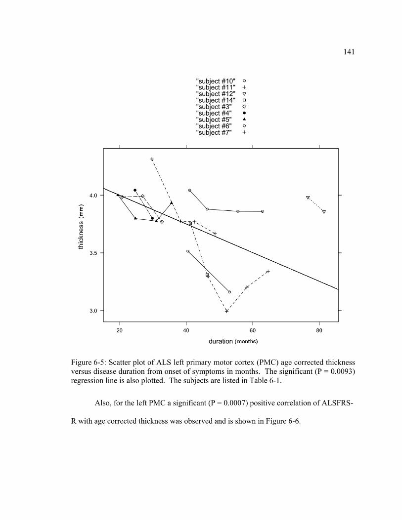
141

Also, for the left PMC a significant (P = 0.0007) positive correlation of ALSFRS-

R with age corrected thickness was observed and is shown in Figure 6-6.

Figure 6-5: Scatter plot of ALS left primary motor cortex (PMC) age corrected thicknessversus disease duration from onset of symptoms in months. The significant (P = 0.0093) regression line is also plotted. The subjects are listed in Table 6-1.

142

Figure 6-6: Scatter plot of ALS left primary motor cortex (PMC) age corrected thicknessversus the Revised ALS Functional Rating Score (ALSFRS-R). The significant (P = 0.0007) regression line is also plotted. The subjects are listed in Table 6-1.

The left PCG showed a significant (P = 0.0134) negative correlation of thickness

with disease duration and is shown in Figure 6-7.

143

Figure 6-7: Scatter plot of ALS left postcentral gyrus (PCG) thickness versus disease duration from onset of symptoms in months. The significant (P = 0.0134) regression line is also plotted. The subjects are listed in Table 6-1.

144

6.4.3 Regional average cortical thickness and cognitive exams

Cognitive deficiencies in association with cortical thinning are depicted in

T

6 cu

The ALS thickness results in Section 6.4 are mixed and appear contradictory at

fi le present a clearer picture. First, the negative cross-

se el

the average ALS thickness was not significantly thinner than controls and did not

decrease with time, disease duration, or with everity. This can be explained in one of

two ways. First, it’s possible that the thickness estimation technique described in Chapter

Table 6-2: Cortical thinning in association with PSSFTS su ciencies Ssample.

FT

able 6-2.

.5 Dis ssion

rst, but when interpreted as a who

ctional and longitudinal SPM5 thickness map findings indicate that on a regional lev

s

btest defi in an AL

PPS S Subtest ROI

LMT RIOG RMOG RSPL LITG G

CF (N=5) p=0.029 p=0.088

COGNISTA T

CONST 0) p=0.05 (N=1 5

VisM ( p=0.106 p=0.107 p=0.090 N=9)

PSSFTS=Penn State Screen of Frontal and Temporal Dysfunction Syndromes, CF=category fluency,

COGNISTA -D TG=left

rus, left middle temp us, LIOG ft inferior occipital gyrus IOG=rig ior occipital

O t middle occipital gy RSO su cipital gy PL=right superior p bule.

T=Neurobehavioral Cognitive Status Examination, CONST=2 constructions, VisM=visual memory, LI

inferior temporal gy LMTG= oral gyr =le , R ht infer

gyrus, RM G=righ rus, G=right perior oc rus, RS arietal lo

145

4 does ces

e good GM/WM contrast and typically

ultiple averages in order to work well. The thickness estimation technique presented in

Chapter 4 will work with good or poor quality T1-weighted images. The other likely

explanation is heterogeneity of cortical thinning within the patient ALS patient

population. This explanation is likely based on the ROI results presented in Section

6.4.2. When the average thickness of the entire right PMC was compared with controls,

the ALS limb and probable groups were significantly thinner. For the left PMC,

thickness was not significantly thinner than controls, but showed significant correlation

with time, disease duration, and ALSFRS-R. The PCG showed a similar, yet less

dramatic effect for both sides. If ALS population heterogeneity is the explanation for the

negative whole-brain thickness findings, only a very large ALS study cohort will yield

positive results. Furthermore, these results suggest that cortical thinning in ALS is slight

ips for temporal and occipital cortical mediated

capacit the

dial

not have the sensitivity to measure the small submillimeter thickness differen

reported in previous ALS thickness studies [1, 2]. This explanation can be verified by

using the same data with one of the surface-based cortical thickness based methods.

However, the T1-weighted protocol used in this study is suboptimal for surface-based

cortical thickness applications which requir

m

and is not likely to be detected using qualitative methods.

Consistent with recent imaging literature [10, 11], evaluation of the association

between cognitive deficiencies in ALS and cortical thinning shown in Section 6.4.3

evidenced significant relationsh

ies. Category fluency demonstrated a statistically significant association with

left inferior temporal region, approaching significance for association with the left me

temporal region. The COGNISTAT subtest of 2-D constructions approached

146

significance for association with the right inferior occipital region. Trends were further

evident for a drawing task of visual memory in association with the left medial temporal

right inferior occipital, and right medial occipital regions (Table 6-2). The latter is

consistent with the recent work of Jeannerod and co-workers [11]. To date, no known

study has attempted to examine the relationships between a clinically practical cognitive

screen in ALS, brief while sensitive enough to identify FTD sub-types, and quantitativ

imaging data. This study provides pilot data upon which to base larger studies that will

validate the PSSFTS as a diagnostic tool for use in ALS

,

e

Multidisciplinary Outpatient

Clinics

[1] J. A. Butman and M. K. Floeter, "Decreased Thickness of Primary Motor Cortex in Primary Lateral Sclerosis," American Journal of Neuroradiology, vol. 28, pp. 87-91, 2007.

tagliata, L. Bonzano, G. Mancardi, C. Canepa, and C. Caponnetto, f motor cortex thinning and corticospinal tract involvement by

quantitative MRI in amyotrophic lateral sclerosis," Amyotrophic Lateral

[3] M. D. Meadowcroft, J. R. Connor, Z. Simmons, D. C. Bigler, J.-L. Wang, M. B.

Analysis of Primary Motor Neuronal Loss in Amyotrophic Lateral Sclerosis," in

Resonance in Medicine, Seattle, Washington, USA, 2006.

Wang, M. B. Smith, and Q. X. Yang, "Quantitative Magnetic Resonance and

66, p. A186, 2006.

. Brain imaging validation of this screen exam of FTD sub-types will contribute

to the success of approaches to facilitate ALS-FTD patient decision making during

discussions of treatment planning and end-of-life issues.

6.6 References

[2] L. Rocca"Detection o

Sclerosis, 2008.

Smith, and Q. X. Yang, "Quantitative Magnetic Resonance and Histological

Proceedings 14th Scientific Meeting, International Society for Magnetic

[4] M. D. Meadowcroft, X. S. Wang, J. R. Connor, Z. Simmons, D. C. Bigler, J.-L.

Histological Analysis of Primary Motor Neuronal Loss in ALS," Neurology, vol.

147

Simmons, Q. X. Yang, and M. B. Smith, "Gray Matter Thinning Demonstrated in

International Society for Magnetic Resonance in Medicine, Seattle, Washington,

[6] K. R. Scott, D. Bigler, H. E. Stephens, Q. X. Yang, and Z. Simmons, "A Novel

Neurology, vol. 66, p. A245, 2006.

MRI post-processing on a supercomputer," Computer Methods and Programs in

[8] C. Davatzikos, A. Genc, D. Xu, and S. M. Resnick, "Voxel-Based Morphometry

Longitudinal Atrophy," NeuroImage, vol. 14, pp. 1361-1369, 2001.

battery to identify frontal dysfunction in patients with ALS," Neurology, vol. 67,

[10] A. L. R. Adlam, K. Patterson, T. T. Rogers, P. J. Nestor, C. H. Salmond, J.

progressive aphasia: two sides of the same coin?," Brain, vol. 129, pp. 3066-3080,

[11] M. Jeannerod and P. Jacob, "Visual cognition: a new look at the two-visual

[5] D. C. Bigler, K. R. Scott, M. D. Meadowcroft, J. X. Wang, H. E. Stephens, Z.

ALS Using Novel Thickness Maps," in Proceedings 14th Scientific Meeting,

USA, 2006, p. 728.

MRI Technique Demonstrates Thinning of Primary Motor Cortex in ALS,"

[7] D. C. Bigler, Y. Aksu, and Q. X. Yang, "STAMPS: software tool for automated


Using the RAVENS Maps: Methods and Validation Using Simulated

[9] C. Flaherty-Craig, P. Eslinger, B. Stephens, and Z. Simmons, "A rapid screening

pp. 2070-2072, 2006.

Acosta-Cabronero, and J. R. Hodges, "Semantic dementia and fluent primary

2006.

systems model," Neuropsychologia, vol. 43, pp. 301-312, 2005.

Chapter 7

ALS Brain Volumetric Analysis

7.1 Abstract

Objective:

Perform BPF, VF, and VBM in ALS cross-sectionally and longitudinally to characterize

whole-brain and regional atrophy in ALS by group, disease duration, severity, and time.

Methods:

T1-weighted MRI was acquired from 14 control and 14 ALS at baseline, 8 at 6 months, 6

at 12 months, and 4 at 18 months. STAMPS was used to label VENT and generate

RAVENS GM, WM, and VENT images. BPF and VF were calculated using segmented

images. SPM5 was used for whole-brain statistical analysis. R was used for BPF and VF

statistics.

Results:

Average 0.24%/month BPF decrease for disease duration in generalized (limb and

bulbar) group was significant (P = 0.0425). Difference in VF between ALS at baseline

and controls approached significance (P = 0.09827). Average 0.009%/month VF increase

for duration and time was significant (P = 0.0576, P = 0.0528). Regional atrophy in GM

and WM correlated with duration and time in frontal, temporal, motor, parietal, and

occipital regions.

Conclusions:

149

VF appears more sensitive for monitoring disease progression than BPF. Generali

ALS is more likely to show BPF decrease with disease duration. Regional results show

atrophy throughout CNS in both GM and WM. The clinical measure of severity

correlates poorly with atrophy.

zed

150

7.2 Introduction

As discussed in Chapter 5, currently ALS remains a clinical diagnosis. In many

cases, an exhaustive evaluation is undertaken to rule out other diseases. Thus, there is a

pressing need for development of clinically useful and readily available imaging

biomarkers of ALS. Cross-sectional whole-brain VBM (Chapter 2, Section 2.4.1.1) has

been used to address this need. As mentioned in Chapter 5, Section 5.5.5, an examination

of the VBM results show

,

clinical scores of disease se

s GM atrophy in motor [1-6], frontal [1-4, 6-8], temporal [1-4],

parietal [1], and occipital [1] regions in ALS subjects when compared with normal

controls. WM density was also shown to decrease in the CST [5, 6] and the subcortical

frontal [5-7], temporal [2], and occipital [3] regions. As pointed out by Filippi et al [4]

the fact that volume loss occurs in frontal and temporal regions for ALS patients with and

without FTLD, warrants longitudinal VBM studies for prognostic purposes. However, to

date only one longitudinal VBM study of ALS has been performed [5]. Also, BPF

(Chapter 2, Section 2.4.1) was used to show significant whole-brain volume decreases in

ALS subjects when compared to controls [2, 8, 12], but BPF did not correlate with

verity or duration. Longitudinal measurements of BPF are

needed to determine the rate of BPF decrease and how it correlates with disease severity

and duration. In addition, VF (Chapter 2, Section 2.4.1) was shown to be greater in ALS

when compared with controls [6], but has no yet been investigated longitudinally. To

address these needs, a cross-sectional and longitudinal BPF, VF, and VBM study for GM,

151

WM, and VENT was performed and is presented in this Chapter.


7.3.1 Subjects

See Chapter 6, Section 6.3.1 for the subject information.

ction 6.3.2 for the MRI protocol.

7.3.3 Image post-processing

h

e

7.3.2 MR-Imaging protocol

See Chapter 6, Se

Image post-processing was performed using STAMPS (Chapter 3) [7]. As

described in Chapter 3, Section 3.5, the baseline ALS and normal control RAVENS

images were normalized to remove individual whole-brain volume bias in the cross-

sectional VBM analysis. For longitudinal VBM analysis, the baseline image for eac

ALS subject was used as the target atlas for generating the RAVENS image and then th

outputs were registered to the HAMMER supplied brain atlas using HAMMER. The

main purpose for using HAMMER was to minimize registration error for subsequent

whole-brain VBM analysis [8, 9].

152

7.3.4 C

The R statistical software package (http://www.r-project.org/

ross-sectional and longitudinal BPF and VF analysis

) was used for the

brain images with the cerebellum and brainstem removed. Similarly, VF was calculated

paired t-test was used to test for a significant decrease in BPF and increase in VF between

used to test correlation of BPF and VF with time from baseline and ALSFRS-R. A

BPF and VF with disease duration from onset of symptoms. All ALS subjects that

hole-brain voxel-based statistical analysis for RAVENS images was performed

using SPM5. Prior to analysis the images were smoothed with a 5 mm FWHM Gaussian

kernel and an explicit mask was generated from the average smoothed image of all of the

subjects by iteratively increasing a minimum threshold value such that the final mask

BPF and VF statistical analyses. BPF was calculated as the sum of the volumes of GM

and WM divided by the sum of the volumes of GM, WM, and CSF using the segmented

by dividing the VENT volume by the sum of the volumes of GM, WM, and CSF. A

ALS baseline and controls.

A linear mixed effects analysis with time from baseline as the random effect was

similar model was used with disease duration as the random effect to test correlation of

completed at least two scans were included in the analysis. ALS subjects were grouped

by limb, bulbar, and generalized. Linear regression of BPF and VF with age in years was

performed on the control subjects and the average slope was used to correct the

longitudinal ALS BPF and VF values prior to statistical analysis.

7.3.5 Cross-sectional and longitudinal whole-brain VBM analysis

W


153

only contained the target tissue (i.e. GM, WM, or VENT). The kernel size was chosen

based on the minimum size used in the validation of RAVENS [10].

leaving

signific

value o

longitu

conditi dom

16

months

covaria imaged on all three time points were included

in the t

ag by

m

lysis,

longitu s identified using the

HAMM

A paired t-test (14 conditions, 2 blocks, 16 total having 15 degrees of freedom,

13 degrees of freedom from 28 images) was used to locate brain regions with

antly less volume density in baseline ALS when compared to age-matched NC’s.

These regions were highlighted by thresholding the statistic maps with an uncorrected p-

f 0.001. The minimum cluster size was set to 50 voxels.


dinal ALS image data. In all four models, the independence option was set to


ons, 2 blocks, 10 total having 9 degrees of freedom, leaving 7 degrees of free

from images) between baseline and 6 months ALS was performed. The remaining

odels were full factorial designs grouped bthree m y baseline ALS, 6 months ALS, and 12

ALS with time, disease duration from onset of symptoms, and ALSFRS-R as

tes. Only those subjects that were

hree groups (3 conditions, 1 covariate, 4 total having 11 degrees of freedom from

15 im es for each model). Statistically significant brain regions were highlighted

thresholding the statistic maps using a false discovery rate (FDR) of 0.05 and a minimu

cluster size of 50 voxels.

Also, using the significant clusters identified in the cross-sectional ana

MARSBAR [11] was used to query the four previously described models for significant

dinal effects. The anatomical label of each region wa

ER supplied labeled atlas. Regions that were identified as lying mostly outside

154

the tiss e loss in

m

by divi

during S generation and the multiplication by the number of voxels in the cluster

conver

7.4 Res

7.4.1 C

subject

analysi s with time and ALSFRS-R were not significant. A significant

duratio group existed.

Figure

groupe

sympto

ue of interest were ignored. For the RAVENS images, the average volum

mm3/ onth for time and disease duration and mm3/score for ALSFRS-R were calculated

ding the correlated slope by 20 and multiplying the result by the number of voxels

in the cluster. The division by 20 removes the default scaling applied by HAMMER

RAVEN

ts mm3/voxel (i.e. tissue volume density) to mm3 (i.e. tissue volume).

ults

ross-sectional and longitudinal BPF and VF analysis

The average 0.25% per year negative correlation of BPF with age for the control

s was significant (P = 0.0271). The paired t-test between baseline ALS and

controls showed no significant decrease in BPF (P = 0.8095). For the longitudinal

s, the correlation

n effect (P = 0.0425) for the generalized (i.e. limb and bulbar) ALS

7-1 shows the scatter plot of age corrected BPF versus ALS disease duration

d by limb and generalized. Average BPF decrease as a function of disease

duration for the generalized group was 0.24% per month. Disease duration from onset of

ms was significantly different (P = 0.0463) between the limb (average duration

47.67±15.29 months) and generalized (average duration 30.41±13.69 months) groups.

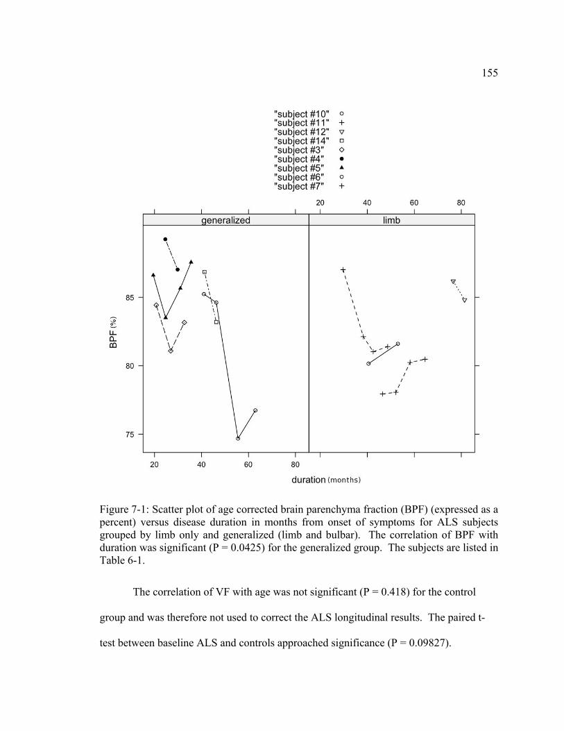
155

Figure 7-1: Scatter plot of age corrected brain parenchyma fraction (BPF) (expressed as a percent) versus disease duration in months from onset of symptoms for ALS subjects grouped by limb only and generalized (limb and bulbar). The correlation of BPF with duration was significant (P = 0.0425) for the generalized group. The subjects are listed inTable 6-1.

The correlation of VF with age was not significant (P = 0.418) for the control

group and was therefore not used to correct the ALS longitudinal results. The paired t-

test between baseline ALS and controls approached significance (P = 0.09827).

156

Longitudinally, a significant time (P = 0.0576) and duration (P = 0.0528) effect were

observed. Figure 7-2 shows the scatter plot of VF versus time and Figure 7-3 shows the

scatter plot of VF versus disease duration. Average VF increase per month, which was

approximately the same for disease duration and time, was 0.009% per month. The ALS

d ALSFRS-R were not significant. group effect an

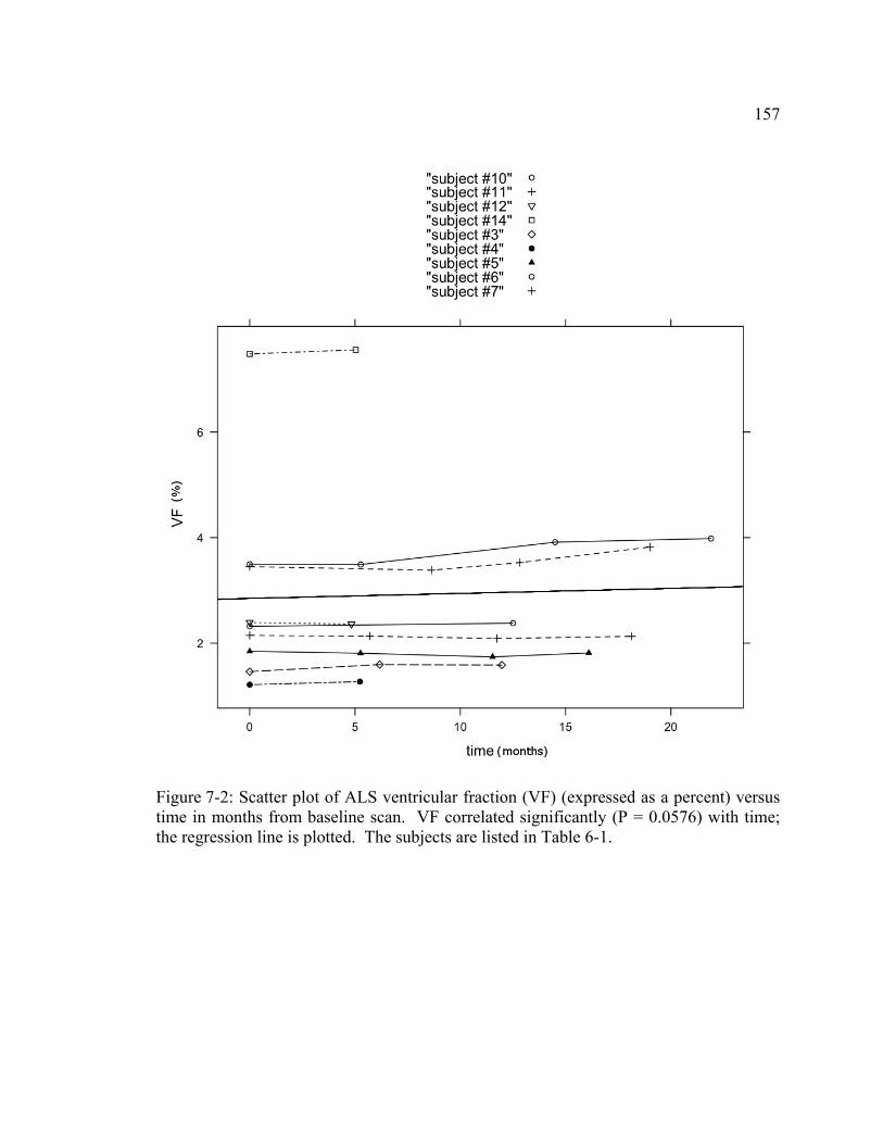
157

Figure 7-2: Scatter plot of ALS ventricular fraction (VF) (expressed as a percent) versus time in months from baseline scan. VF correlated significantly (P = 0.0576) with time; the regression line is plotted. The subjects are listed in Table 6-1.

158

Figure 7-3: Scatter plot of ALS ventricular fraction (VF) (expressed as a percent) versusdisease duration in months from onset of symptoms. VF correlated significantly (P =0.0528) with duration; the regression line is also plotted. The subjects are listed in Table

6-1.

159

7.4.2 Cross-sectional and longitudinal whole-brain VBM analysis

Significant clusters were identified in the RAVENS GM and WM images,

whereas no clusters were identified

respectively.

for RAVENS VENT images. Figure 7-4 and

Figure 7-5 show the cross-sectional results for the RAVENS GM and WM images

160

Figure )

e

7-4: Orthogonal views of RAVENS GM for brain regions listed in Table 7-1: (aright precentral gyrus overlapping onto right postcentral gyrus, (b) left postcentral gyrus,(c) left superior parietal lobule, (d) right superior parietal lobule, (e) right middltemporal gyrus, (f) right middle temporal gyrus, (g) left middle temporal gyrus, (h) rightlateral fronto-orbital gyrus overlapping onto left lateral fronto-orbital gyrus, and (i) left

The t-values (0.001 uncorrected p-value and 50 voxel extent) the smoothed average RAVEN GM image for all subjects.

lateral fronto-orbital gyrus. are overlaid on

161

Figure 7-5: Orthogonal views of RAVENS WM for brain regions listed in Table 7-1: (a) left par ftparietal lobe WM near left superior parietal lobule, (c) left parietal lobe WM near left

poralgyrus, (e) right parietal lobe WM near right postcentral gyrus, (f) right parietal lobe WM

ietal lobe WM near left postcentral gyrus and superior parietal lobule, (b) le

angular and supramarginal gyri, (d) right temporal lobe WM near right middle tem

near right postcentral gyrus, (g) left frontal lobe WM near left medial frontal andprecentral gyri, and (h) left frontal lobe WM near left precentral gyrus. The t-values

RAVEN WM image for all subjects. (0.001 uncorrected p-value and 50 voxel extent) are overlaid on the smoothed average

Table 7-1 summarizes the longitudinal results using the significant clusters shown

in Figures 7-4 and 7-5. When compared to controls, significant GM volume loss

162

occurred within motor, temporal, lateral frontal-orbital, and parietal regions. Significant

WM volume loss was found in parietal, temporal, and frontal lobes.

163

Table 7-1: P-values and average volume loss for cross-sectional regions applied to longitudinal ALS RAVENS GM and WM statistical modeshown only for regions that are significant or that approac

ls. Average volume loss ished significance (p-value <

0.10). Paired t-test Time Duration ALSFRS-R Tissue Brain

Loss (mm3/month) (mm3/month)

s

(mm3/score)

Region p-value Volume

(mm3)

p-value Volume Loss p-value Volume Loss p-value Volume Los

GM(a) Right PMC 0.4104 - 0.0046 6.2985 0.9984 - 0.7939 -

GM(b) Left PCG 0.0600 2.6797 0.9966 - 0.0540 0.1550 0.0007 0.4340

GM(c) Left SPL 0.0637 3.1080 0.2339 - 0.6562 - 0.9161 -

GM(e) Right

MTG

0.8617 - 0.3200 - 0.0328 0.1580 0.1925 -

GM(f) Right

MTG

0.0604 7.1550 0.0005 7.8175 0.2355 - 0.0654 1.1925

GM(h)

GM(d) Right SPL 0.1319 - 0.2577 - 0.0012 0.4895 0.0691 0.4005

GM(g) Left MTG 0.2313 - 0.1315 - 0.0000 1.4260 0.9127 -

Right

LFOG

0.0045 4.4000 0.1975 - 0.6913 - 0.6662 -

GM(i) -

WM(d) Right TL 0.1386 - 0.0000 2.9120 0.7588 - 0.5070 -

PMC = primary motor cortex, PCG = postcentral gyrus, SPL = superior parietal lobule, MTG = middle temporal gyrus, LFOG = lateral fronto-

Left LFOG 0.2101 - 0.0004 3.0805 0.9104 - 0.5467

WM(a) Left PL 0.9522 - 0.4643 - 0.8979 - 0.7754 -

WM(b) Left PL 0.1647 - 0.0357 2.0915 0.9980 - 0.2775 -

WM(c) Left PL 0.0487 2.0915 0.0091 2.1360 0.3006 - 0.0599 0.4005

WM(e) Right PL 0.0148 2.7540 0.0094 1.3770 0.0344 0.3780 0.7289 -

WM(f) Right PL 0.0666 1.7680 0.0319 1.2250 0.0000 0.8580 0.0805 0.3000

WM(g) Left FL 0.0023 3.3325 0.0349 0.9750 0.2520 - 0.9599 -

WM(h) Left FL 0.1077 - 0.6284 - 0.0219 0.7625 0.9863 -

orbital gyrus, PL = parietal lobe, TL = temporal lobe, FL = frontal lobe

Paired t-test = baseline ALS and 6 month paired t-test.

Time = time since baseline using ALS subjects that completed baseline, 6 month, and 12 month time-points correlated with volume.

Duration = disease duration from onset of symptoms using ALS subjects that completed baseline, 6 month, and 12 month time-points correlated

ALSFRS-R = ALS Functional Rating Score-Revised using ALS subjects that completed baseline, 6 month, and 12 month time-points correlated

with volume.

with volume.

164

Figures 7-6(a) and 7-6(b) show the significant clusters identified in the four

longitudinal models for the RAVENS GM and WM images respectively. No signifi

clusters were found using the model with ALSFRS-R as a covariate in either RAV

GM or WM images. For RAVENS GM images only, no significant clusters were found

using the mode

cant

ENS

l with time as a covariate.

The paired t-test between baseline and 6 month ALS RAVENS GM images

yielded clusters of significant volume loss in the left inferior frontal gyrus (IFG), left

supramarginal gyrus (SMG), left middle frontal gyrus (MiFG), left superior temporal

Figure 7-6: 3D views of longitudinal (a) RAVENS GM and (b) RAVENS WM results.Red clusters show significant (0.05 false discovery rate and 50 voxel extent) decrease involume using the paired t-test between baseline and 6 month ALS subjects, green clustersshow significant negative correlation of volume with disease duration from onset of symptoms, and blue clusters show significant negative correlation of volume with timefrom baseline.

165

gyrus (STG), left lingual gyrus (LG), left PMC, left insula, left medial occipitotemporal

between baseline and 6 months was found in small bilateral regions within the frontal

lobes. Negative correlation of volume with time was mainly located in the frontal lobes

(FL’s) bilaterally, but large clusters were also found in the bilateral temporal lobes

(TL’s), and the left parietal lobe (PL). Finally, negative correlation of volume with

disease duration from onset of symptoms was found in the right FL, bilateral TL, right

PL, and left occipital pole.

se duration between the studies. However, the average disease

duratio and in

months, which are all considered to be in the latter stages

gyrus (MOTG), and right hippocampal formation. Negative correlation of GM volume

with disease duration from onset of symptoms was detected in the bilateral MiFG,

bilateral PMC, bilateral lateral fronto-orbital gyri, bilateral cingulate regions, bilateral

superior frontal gyri, bilateral SMG, bilateral medial frontal gyri (MeFG), bilateral STG,

bilateral middle temporal gyri (MTG), bilateral PCG, bilateral MOTG, right caudate

nucleus, right cuneus, right superior parietal lobule (SPL), left IFG, left LG, left superior

occipital gyrus, left insula, and left angular gyrus (AG).

For the ALS RAVENS WM images, significant volume loss for the paired t-test

7.5 Discussion

Contrary to previous studies [3, 6, 12], BPF was not significantly reduced in ALS

subjects when compared with controls. It’s possible to explain this contradiction based

on differences in disea

ns were 20.5 months [6], 24 months [3], 38.1 (range, 8 – 89) months [12],

this study 39.0 (range, 15 – 77)

166

of the disease. Therefore, the difference is likely due to the patient populations used in

each study. Kassubek et al [3] selected only patients who met the El Escorial criteria for

ALS definite, Mezzapesa et al [12] selected ALS probable or ALS definite, and in this

study ALS suspected, probable, and definite were included. Frank et al [6] did not use

th scorial c used a large nt population of 74 ALS subjects grouped by

sp d bulba e therefore b umed that given a large patient population,

in g suspec icantly less than norm l contr

Regardless, as pointed out by Mezzapesa et al [12], whole-brain atrophy in ALS is mild.

In evious s ies no correlation o with ALSFRS and d ease du were

found, whereas in this study a negative correlation of BPF with disease duration for the

ge in

the limb group. This suggests that patients with bulbar onset ALS are more likely to

show global brain volume reduction sooner with disease duration; although examination

7-1 shows that subject #10 is likely the main cause for

this significant finding. Subject #10 showed a sudden drop of BPF from 84% to 74%

between the second and third scans and then leveled out again at 76% on the fourth scan.

ent in ALS when

compar

sing

ts

e El E riteria, but patie

inal an r. It can b e ass

cludin ted ALS, BPF will be signif a ols.

the pr tud f BPF is ration

neralized group was found. Interestingly, disease duration was significantly greater

of the generalized group in Figure

VF showed a significant trend towards ventricular enlargem

ed with controls and VF increased significantly with both time and disease

duration. This suggests that VF might be a more sensitive indicator of ALS disease

progression than BPF. Frank et al [6] showed a similar cross-sectional finding u

lower resolution images and manual labeling.

The correlation of VF with age was not significant for the control subjects. This

is contrary to a recent VF study in aging [13]. However, the average age of the subjec

167

in the referenced study was 72.7 ± 3.56 years; on average older than the NC’s used in this

study (56.0 ± 13 years). In addition the sample size was much larger (> 150 subjects)

than the sample size in this study. Therefore, this discrepancy is likely due to differen

in age and sample size. Since ALS VF was not age corrected, the significant longitudinal

increase of VF over time might be attributed to age. This is not likely, because the

average annual increase of VF for ALS of 0.108% is larger than the approximate 0.025

average annual increase for the older norm

ces

%

al control subjects studied previously (see

Figure 2(a))[13].

Using RAVENS VENT images no significant results were seen cross-sectionally

or longitudinally. This result is not surprising in light of the VF findings. RAVENS

VENT images are used to find regional differences in ventricular volume density. First,

since VF only approached significance cross-sectionally, one would not expect to find

regions of significantly increased volume density in RAVENS VENT images cross-

sectionally. Second, VF increased longitudinally, but no significant longitudinal effect

was seen in RAVENS VENT images. This merely suggests that ventricular enlargement

in ALS is not confined to a particular region within the ventricles for every subject in this

study and therefore a larger ALS patient population would be needed to detect a

significant longitudinal effect using RAVENS VENT and VBM.

Cross-sectional WM VBM results vary widely in the literature. Positive results

show volume loss in the CST [2, 7], frontal [2, 7, 9], temporal [2], and occipital [3]

regions and an equal number report no findings at all [1, 3, 5]. Differences in patient

populations and small cohort sizes likely play a role in this variance, but differences in

image acquisition and processing are often overlooked and can alter the findings

168

considerably. It has been shown that varying the smoothing kernel size alone for

statistical parametric maps can generate multiple results for a single data set [14]. The

minimal kernel smoothing size and improved VBM technique used in this study were

chosen to address this problem. This study demonstrated WM volume loss both cross-

sectionally and longitudinally, in parietal, occipital, frontal, and temporal lobes. Cross-

sectionally regions of volume loss were identified in RAVENS WM mainly in parietal

and frontal areas. Longitudinally with time, significant volume loss was identified

mainly in subcortical frontal and temporal WM regions. The paired t-test of baseline and

6 months ALS, which included all of the subjects who returned for their second visit,

showed bilateral frontal volume loss only.

As expected, ALS RAVENS GM showed bilateral volume decrease in the PMC

and PCG when compared with controls. The right PMC was the largest cluster and

therefore demonstrated larger volume loss over the duration of the longitudinal study (see

Table 7-1). The only other VBM study to include El Escorial suspected ALS patients,

also reported bilateral volume loss in motor areas [15], but due to the small patient size

used in this study, it was not possible to determine regional cortical volume decrease in

ALS based on El Escorial criteria. However, the volume loss between ALS and controls

loss in the PMC [3, 5]. In a previous MRI and histological report on 4 freshly excised

LS cadaver brains, it was demonstrated that the motor cortex was not thinner when

compared with frontal and occipital cortices [16, 17]. In the study, Nissl stained 20 µm

in the PMC did not correlate with disease duration or ALSFRS-R longitudinally in ALS

as might be expected. This might be due to the ALS subjects who did not return for

subsequent scans after baseline. Moreover, not all VBM studies have reported volume

A

169

thick tissue samples showed decreased neuronal density and the high-resolution (0.78 x

compared with other brain regions, but changes in the cell body shape were observed

[20]. Based on these results, it would appear that in some cases the detected VBM

volume loss in the motor cortex is more likely due to “apparent” cortical thinning due to

loss of T1-weighted image contrast in GM and WM [21-23]. Further histological and

imaging studies are needed to validate these findings.

The paired t-test between baseline and 6 months ALS RAVENS GM showed

regions of volume loss predominantly in gyri of the left hemisphere (with the exception

of the right hippocampal formation) and located in frontal, temporal, motor, and parietal

regions. These results are similar with the only other longitudinal ALS VBM study to

date [5], which showed decreases in GM volume in motor, parietal, and frontal areas that

extended to cingulate areas and cerebellum after 6 months. Similar regions were also

detected in this study when volume was correlated with disease duration from onset of

symptoms. These results support the notion that extramotor upper motor neuron

involvement is prevalent in ALS and ALS-FLTD.

Although, complete cognitive tests at time of imaging were not available for all

the subjects included in this study, most subjects were administered the PSSFTS [24].

Five of the 14 baseline ALS and 2 of the 5 ALS included in the whole-brain longitudinal

analyses showed signs of FLTD. Subject #14 was completely mute for both scan dates.

Notably, volume loss was statistically significant in the left IFG for both the RAVENS

0.78 x 1.00 mm, 8 averages) T -weighted images showed loss of contrast between GM

and WM in the motor cortex when compared to other gyri. Other histological studies

showed that the number [18] and size [19] of cortical neurons were not different when

1

170

GM paired t-test between baseline and 6 month ALS and correlation with ALS disease

duration. The left IFG appears to be a common site of volume loss for ALS as previous

ALS VBM studies have demonstrated [2-4, 6]. The left IFG was shown to be associated

w ge wor ] era rt

m e o function [26, 27]. Also, the right MTG

was the only area where volume loss was detected LS in AVENS GM and

WM. Functional neuroimaging studies have sugg hat th dle temp yrus is

i d in lan antic memory processing [28-30 addition, Chapter 6,

Section 6.4.3 d ated correla f cortical ng wi nitive e cores in

t al brain

As dem d in Table 7 sing the re identi n the cro ctional

a , ALSFRS-R correlated w inal ENS GM volume loss in the left

PCG, right SPL, and right MTG. In RAVENS W SFRS elated olume

loss in the left G MG and the right PL near the right PCG.

However, whole-brain longitudinal correlation of ALSFRS-R t signi for any

o

significantly (P = 0.0021) for this group of subjects over the duration of the study.

G in the

right MeFG using GM VBM, but no other VBM studies have shown similar findings.

This suggests that there is a weak association between ALSFRS-R and upper motor

neuron volum er longitudinal patient cohort is required to substantiate

t

ith langua production and d retrieval [25 and bilat lly as suppo for

aintenanc f attentional focus and executive

in A both R

ested t e mid oral g

nvolve guage and sem ]. In

emonstr tion o thinni th cog xam s

empor regions.

onstrate -1, u gions fied i ss-se

nalysis ith longitud RAV

M AL -R corr with v

PL near the left A and S

was no ficant

f the image types (RAVENS GM, WM, VENT), even though ALSFRS-R decreased

rosskreutz et al [15] reported correlation of ALSFRS-R with volume loss only

e loss. Again, a larg

hese findings.

171

Finally, a comment must be made on the challenges and limitations of this study.

First, ALS patient dropout for the longitudina

to finish the study or not. When comparing ALSFRS-R, age, and disease duration

demographic measures seemed to predict whether or not the patient was able to finish the

whole-brain statistical analysis. Future

longitudinal studies involving ALS will need to either select patients in the early stages of

brain regions specific to FTLD was shown, but a comprehensive longitudinal correlation

l study was large and difficult to predict.

Only 2 subjects dropped out of the study for reasons other than disease progression or

death. During patient selection it was difficult to predict whether patients would be able

between the last acquired set of data for subjects that dropped out (25.9 ± 10.4, 56.7 ±

15.3 years, 38.8 ± 12.5 months) and the same parameters for the subjects who finished

the study (32.8 ± 5.7, 58.7 ± 9.6 years, 53.0 ± 13.6 months), no significant differences

were found (P = 0.17265, P = 0.792, P = 0.1341). Therefore, none of the clinical and

study. Second, linear mixed effects statistical analysis, which can handle the missing

data problem, is available for standard statistical packages, but is not available for whole-

brain statistical parametric mapping based on the general linear model. This meant that

not all of the subjects could be used for

the disease or shorten the duration between image acquisitions. Last, volume loss in

of cognitive exams and volume loss was not performed. This is necessary to be able to

understand and possibly predict FLTD within ALS.

172

7.6 References

[1] L. Thivard, P.-F. Pradat, S. Lehericy, L. Lacomblez, D. Dormont, J. Chiras, H. Benali, and V. Meininger, "Diffusion tensor imaging and voxel based morphometry study in amyotrophic lateral sclerosis: relationships with motor disability," Journal of Neurology, Neurosurgery, and Psychiatry, vol. 78, pp. 889

[2] S. Abrahams, L. H. Goldstein, J. Suckling, V. Ng, A. Simmons, X. Chitnis, L. Atkins, S. C. R. Williams, and P. N. Leigh, "Frontotemporal white matter changes in amyotrophic lateral sclerosis," Journal of Neurology, vol. 252, pp. 321-331,

[3] J. Kassubek, A. Unrath, H. J. Huppertz, D. Lule, T. Ethofer, A. D. Sperfeld, and A. C. Ludolph, "Global brain atrophy and corticospinal tract alterations in ALS, as investigated by voxel-based morphometry of 3-D MRI," Amyotrophic LateraSclerosis and Other Motor Neuron Disorders, vol. 6, pp. 213-220, 2005.

[4] M. Filippi, F. Agosta, and M. A. Rocca, "Regional Assessment of Brain At

-892, 2007.

2005.

l

rophy: A Novel Approach to Achieve a More Complete Picture of Tissue Damage Associated with Central Nervous System Disorders?," American Journal of Neuroradiology, vol. 28, pp. 260-261, 2007.

[5] J. Grosskreutz, C. Keil, L. Emmerich, R. Dengler, and T. Peschel, "ALS upper motoneuron involvement in DTI and VBM: A longitudinal MRI study," Clinical Neurophysiology, vol. 118, p. e36, 2007.

[6] B. Frank, J. Haas, J. H. Heinze, E. Stark, and T. F. Munte, "Relation of neuropsychological and magnetic resonance findings in amyotrophic lateral sclerosis: evidence for subgroups," Clinical Neurology and Neurosurgery, vol. 99, pp. 79-86, 1997.

[7] D. C. Bigler, Y. Aksu, and Q. X. Yang, "STAMPS: software tool for automated MRI post-processing on a supercomputer," Computer Methods and Programs in Biomedicine, vol. Accepted for Publication, 2009.

[8] F. L. Bookstein, ""Voxel-Based Morphometry" Should Not Be Used with Imperfectly Registered Images," NeuroImage, vol. 14, pp. 1454-1462, 2001.

[9] C. Davatzikos, "Why voxel-based morphometric analysis should be used with great caution when characterizing group differences," NeuroImage, vol. 23, pp. 17-20, 2004.

analysis using an SPM toolbox," in 8th International Conference on Functional Mapping of the Human Brain, Sendai, Japan, 2002.

[12] D. M. Mezzapesa, A. Ceccarelli, F. Dicuonzo, A. Carella, M. F. De Caro, M. Lopez, V. Samarelli, P. Livrea, and I. L. Simone, "Whole-Brain and Regional

[10] C. Davatzikos, A. Genc, D. Xu, and S. M. Resnick, "Voxel-Based Morphometry Using the RAVENS Maps: Methods and Validation Using Simulated Longitudinal Atrophy," NeuroImage, vol. 14, pp. 1361-1369, 2001.

[11] M. Brett, J.-L. Anton, R. Valabregue, and J.-B. Poline, "Region of interest

173

Brain Atrophy in Amyotrophic Lateral Sclerosis," American Journal of

[13] O. T. Carmichael, L. H. Kuller, O. L. Lopez, P. M. Thompson, R. A. Dut

J. T. Becker, "Ventricular volume and dementia progression in the Cardiovascula

[14] D. K. Jones, M. R. Symms, M. Cercignani, and R. J. Howard, "The effect of filter

2005.

Peschel, "Widespread sensorimotor and frontal cortical atrophy in Amyotroph

[16] M. D. Mea

Neuroradiology, vol. 28, pp. 255-259, 2007. ton, A.

Lu, S. E. Lee, J. Y. Lee, H. J. Aizenstein, C. C. Meltzer, Y. Liu, A. W. Toga, and r

Health Study," Neurobiology of Aging, vol. 28, pp. 389-397, 2007.

size on VBM analyses of DT-MRI data," NeuroImage, vol. 26, pp. 546-554,

[15] J. Grosskreutz, J. Kaufmann, J. Fradrich, R. Dengler, H.-J. Heinze, and T. ic

Lateral Sclerosis," BioMed Central Neurology, vol. 6, p. 17, 2006. dowcroft, J. R. Connor, Z. Simmons, D. C. Bigler, J.-L. Wang, M. B.

Smith, and Q. X. Yang, "Quantitative Magnetic Resonance and Histological

Proceedings 14th Scientific Meeting, International Society for Magnetic

[17] M. D. Meadowcroft, X. S. Wang, J. R. Connor, Z. Simmons, D. C. Bigler, J.-L. nd

Histological Analysis of Primary Motor Neuronal Loss in ALS," Neurology, vol.

[18] O. Gredal, H. Pakkenberg, M. Karlsborg, and B. Pakkenberg, "Unchanged total

a stereological study," Journal of Neuroscience Methods, vol. 95, pp. 171-176,

[19] M. H. Toft, O. Gredal, and B. Pakkenberg, "The size distribution of neurons in the 7, pp.

399-407, 2005. ns in

amyotrophic lateral sclerosis," Brain, vol. 116, pp. 203-215, 1993.

Simmons, Q. X. Yang, and M. B. Smith, "Gray Matter Thinning Demonstrated in ng,


[22] D. C. Bigler, Q. X. Yang, and M. B. Smith, "A Simple Method for the Automatic


[23] K. R. Scott, D. Bigler, H. E. Stephens, Q. X. Yang, and Z. Simmons, "A Novel

Neurology, vol. 66, p. A245, 2006.

battery to identify frontal dysfunction in patients with ALS," Neurology, vol. 67,

Analysis of Primary Motor Neuronal Loss in Amyotrophic Lateral Sclerosis," in

Resonance in Medicine, Seattle, Washington, USA, 2006.

Wang, M. B. Smith, and Q. X. Yang, "Quantitative Magnetic Resonance a

66, p. A186, 2006.

number of neurons in motor cortex and neocortex in amyotrophic lateral sclerosis:

2000.

motor cortex in amyotrophic lateral sclerosis," Journal of Anatomy, vol. 20

[20] J. A. Kiernan and A. J. Hudson, "Changes in shapes of surviving motor neuro

[21] D. C. Bigler, K. R. Scott, M. D. Meadowcroft, J. X. Wang, H. E. Stephens, Z.

ALS Using Novel Thickness Maps," in Proceedings 14th Scientific Meeti

USA, 2006, p. 728.

Measurement of Cortical Thickness," in Proceedings 14th Scientific Meeting,

USA, 2006, p. 1608.

MRI Technique Demonstrates Thinning of Primary Motor Cortex in ALS,"

[24] C. Flaherty-Craig, P. Eslinger, B. Stephens, and Z. Simmons, "A rapid screening

pp. 2070-2072, 2006.

174

Perani, and F. Fazio, "Functional heterogeneity of left inferior frontal cortex as

[26] E. R. Sowell, P. M. Thompson, S. E. Welcome, A. L. Henkenius, A. W. Toga,

attention-deficit hyperactivity disorder," The Lancet, vol. 362, pp. 1699-1707,

[27] K. Rubia, A. B. Smith, M. J. Brammer, and E. Taylor, "Right inferior prefrontal

for error detection," NeuroImage, vol. 20, pp. 351-358, 2003.

conceptual knowledge," Neuropsychologia, vol. 35, pp. 1319-1327, 1997.

temporal cortex for perceiving and knowing about objects," Nature Neuroscience,

[30] R. Cabeza and L. Nyberg, "Imaging Cognition II: An Empirical Review of 275 RI Studies," Journal of Cognitive Neuroscience, vol. 12, pp. 1-47,

2000.

[25] E. Paulesu, B. Goldacre, P. Scifo, S. Cappa, M. C. Gilardi, I. Castiglioni, D.

revealed by fMRI," NeuroReport, vol. 8, pp. 2011-2016, 1997.

and B. S. Peterson, "Cortical abnormalities in children and adolescents with

2003.

cortex mediates response inhibition while mesial prefrontal cortex is responsible

[28] D. Tranel, H. Damasio, and A. R. Damasio, "A neural basis for the retrieval of

[29] L. L. Chao, J. V. Haxby, and A. Martin, "Attribute-based neural substrates in

vol. 2, pp. 913-919, 1999.

PET and fM

Chapter 8

ALS Brain T and DTI Analysis

8.1 Abstract

2

Objective:

of T2 change in ALS cross-sectionally using VBR, determine the

relationship of T2 with time, disease duration, and disease severity longitudinally, and to

par

Metho

1 ei

tion

ulti

MARS

Results

areas a

ific 2

Identify regions

com e these findings with DTI FA and MD.

ds:

T -w ghted, multi spin-echo T2-weighted, and DTI MRI were acquired from 13 controls

and 12 ALS at baseline, 7 at 6 months, and 6 at 12 months. FSL was used for correc

of eddy current artifacts and generation of FA/MD. T2-maps were generated from m

spin-echo images using MRIUtil. Images were registered using STAMPS. SPM5 and

BAR were used for statistical analysis.

:

Clusters of significant T2 increase cross-sectionally were found in frontal and temporal

nd in the right CST at the corona radiata (CR). The right CST at the CR was

sign ant cross-sectionally in all three parametric images. Longitudinally, increased T

176

was associated with disease duration mainly in frontal areas, which overlapped with

similar disease duration associated MD increases.

sions: Conclu

,

but lon LS is likely due to atrophy in

cortica

Cross-sectionally VBR detects regional increases of T2 in ALS not found in FA and MD

gitudinally closely matches MD. Increased T2 in A

l areas and acute inflammation in subcortical regions.

177

8.2 Int

both U

es void

of UM

ar y

for AL

conven

in

examin

not seen in standard T

CST fa

g

echo se

[3 h

is simil

hippoca ecreased R2 in the cerebellum and brain stem in multiple

roduction

ALS is a neurodegenerative disease that destroys both the LMN and UMN

responsible for voluntary muscle control. Diagnosis of ALS relies on the presence of

MN and LMN clinical findings (Chapter 5, Section 5.4). However, autopsy

demonstrate CST degeneration in more than 50% of ALS substudi jects who were

N symptoms [2-5]. As a result, much research has been devoted to ALS UMN

biom ker discovery using neuroimaging [1, 2]. MRI is an ideal neuroimaging modalit

S UMN biomarker discovery because it is non-invasive and provides a wide-array

of structural and quantitative images. As discussed in Chapter 5, Section 5.5.2,

tional MRI has been studied extensively. Hyperintensities within the CST and

tensities in the PMC have been observed in T -weighted imaging. Less wehypo 2 ll

ed is quantitative T2 relaxometry, which has the potential to detect small changes

in T2 2-weighted images. Three ROI studies focused mainly on the

iled to show significant differences between ALS and controls [8-10]. These

s are complicatedfindin by the fact that two of the studies [8, 9] used double-echo spin-

quences to measure T2, which undersample the relaxation curve and are prone to

]. To date, no studies have examined ALS using wherror ole-brain T2 VBR [4], whic

ar to VBM [5], but uses whole-brain T2 or R2 (the inverse of T2) map images

instead of GM density images. VBR has been used to identify increased T2 in the

mpus in epilepsy [4], d

178

syste atrophy of the cerebellar type [6], and increased Tm

lobes, a

dy was to identify regions of increased or decreased T2 in

ALS cross-sectionally using whole-brain VBR, determine the relationship of T2 with

time, disease duration from onset of symptoms, and disease severity longitudinally, and

to compare these findings with DTI FA and MD. Since T2 hyperintensities in the brain

are thought to be related to acute demyelination, edema, or gliosis [8], it is hypothesized

that regions of increased T2 identified using VBR will coincide with regions of decreased

FA or increased MD using VB-DTI [9].


8.3.1 Subjects

The ALS subjects used in this study differ slightly from those used in Chapters 6

and 7. Similar to the referenced chapters, ALS patients that met the revised El Escorial

diagnostic criteria for definite, probable, probable lab-supported, or suspected (Chapter 5,

Section 5.4) were recruited from the Penn State Milton S. Hershey Medical Center ALS

Clinic. However, the oldest two subjects were excluded due to missing DTI data for the

oldest subject and poor age matching of normal control subjects. Therefore, twelve of the

baseline ALS subjects (8 male and 4 female, average age 52.7 ± 10.6 years, range 37 – 68

years) were used. Seven ALS subjects returned for a follow-up visit approximately 6

months after baseline and 6 subjects at approximately 12 months. Table 6-1 summarizes

2 in the parietal lobes, occipital

nd supplementary motor areas in the frontal lobes in autism [7].

The objective of this stu

179

the demographic and disease information for each ALS subject (only subjects #’s 1 – 10

were used in this study).

Thirteen approximately age and gender al control subjects (7 male

and 6 female, average age 53.9 ± 10.8, range 37 – 68 years, P = 0.78) without

udy. All participants

were provided written infor

view Board (Penn State College of Medicine IRB Protocol No.

20473).

,

el head receive

coil. A

, 8 ms

and diffusion gradients applied in 32 non-collinear directions

with b

s

matched norm

neurological or neuromuscular diseases were also recruited for the st

med consent and approval for human research was obtained

from the Institutional Re

8.3.2 MR-Imaging protocol

Images were acquired on a Philips Intera 3.0 Tesla system (Philips Healthcare

Andover, MA, USA) using a body transmit coil and a 6 channel parall

ll images were acquired in the axial plane and the number of contiguous slices

was adjusted to cover the entire skull of each subject.

For T2 relaxometry, multi spin-echo images were acquired with 11 echoes

starting TE, 8 ms echo spacing, 3000 ms TR, and SENSE factor 2. The in-plane matrix

size was 256 x 256 and the slice thickness was 4 mm. The final image spacing was 0.9 x

0.9 x 4.0 mm.

DTI images were acquired using single-shot spin-echo EPI, 96 ms TE, 7777.56

ms TR, SENSE factor 2.5

= 1000 s/mm2. The in plane matrix size was 96 x 96 and the slice thickness was

2.5 mm. After zero filling to 256 x 256 in plane matrix size, the final image spacing wa

180

0.9 x 0.9 x 2.5 mm.

For image registration purposes, the high-resolution whole-brain T1-weigh

protocol described in Chapter 6, Section

ted

8.3.3 T2

t to the cerebellum in 4 ALS subjects.

The extent and locations of th ages.

l

6.3.2 was also used.

relaxometry processing

After examination for movement artifacts or poor SNR, 1 control multi spin-echo

image set was removed due to severe movement artifacts. The remaining 12 control

subjects (6 male and 6 female, average age 53.2 ± 10.9, range 37 – 68 years, P = 0.91)

were used for cross-sectional analysis. T2-maps were generated using MRIUtil [10],

which uses the MR Parameter Map Suite described in Appendix A. The non-linear

mono-exponential fitting routine based on the Levenberg-Marquardt algorithm [11] was

used.

8.3.4 DTI processing

Prior to processing, the DTI datasets were examined for movement and SENSE

unfolding artifacts. SENSE unfolding artifacts from the eyes were noted within the

cerebellum and white matter brain areas adjacen

e artifacts were not severe enough to exclude these im

However, 3 of the control subjects did not complete the DTI scan. This left 10 contro

subjects (6 male and 4 female, average age 52.3 ± 10.7, range 37 – 65 years, P = 0.93) for

cross-sectional analysis. The Philips datasets were then converted to 4D Analyze image

181

format, thresholded to remove background noise using the method outlined in [12], and

then corrected for eddy current induced image distortions using FSL [13]. As part o

processing, the image with no diffusion gradients (B0 image) was saved as a separate

image for registration and for creation of a brain mask using FSL BET [12, 13]. MD an

FA images were generated from the eddy current corrected 4D Analyze image using

f the

d

FSL

[13].

age of each subject to non-linearly register the

processed D

hole-brain voxel-based analysis

istical parametric analysis was performed using

8.3.5 Image registration

Image registration was performed using STAMPS (Chapter 3). STAMPS

requires a high-resolution T1-weighted im

TI and T2-map images to an atlas. As described in [14], the processed DTI

and T2-map images are registered to the atlas by first linear registration to the T1-

weighted image (in the subject space) using FSL FLIRT [15] and then non-linearly by

applying the HAMMER generated deformation field to the linearly registered DTI and

T2-map images. The final image spacing after registration to the atlas was 1 mm

isotropic. The main purpose for using HAMMER was to minimize registration error for

subsequent whole-brain analysis [16, 17].

8.3.6 Cross-sectional and longitudinal w

Whole-brain voxel-based stat

SPM5. Prior to analysis all images were smoothed with a 5 mm FWHM Gaussian kernel

182

and an ted

as the o smoothing.

ALS

with ag of freedom,

leaving m

from 2 -DTI and VBR. Significant regions were

highlig d a

minimu

MARSBAR [18]. For each significant cluster identified in T2 relaxometry, DTI FA, and

DTI MD, MARSBAR was used to examine group differences in the alternate image

types.


longitudinal ALS image data. In all four models, the independence option was set to


conditions, 2 blocks, 9 total having 8 degrees of freedom, leaving 6 degrees of freedom

from 14 images) between baseline and 6 months ALS was performed. The remaining

three models were full factorial designs grouped by baseline ALS, 6 months ALS, and 12

months ALS with time, disease duration from onset of symptoms, and ALSFRS-R as

covariates. Only those subjects that were imaged on all three time points were included

in the three groups (3 conditions, 1 covariate, 4 total having 11 degrees of freedom from

15 images for each model). Statistically significant brain regions were highlighted by

thresholding the statistic maps using a FDR of 0.05 and a minimum cluster size of 100

voxels.

explicit mask for each image type (DTI FA, DTI MD, and T2-map) was genera

verlap of each registered image prior to

For cross-sectional analysis, an ANCOVA model grouped by control and

e as covariate (2 conditions, 1 covariate, 3 total having 3 degrees

21 degrees of freedom from 24 images for T2-maps and 19 degrees of freedo

2 images for DTI) was used for both VB

hted by thresholding the statistic maps with a p-value of 0.001 uncorrected an

m cluster size of 100 voxels. A subsequent ROI analysis was performed using

183

Also, using the significant clusters identified in the cross-sectional analysis,

MARSBAR was used to query the fou escribed models for significant

longitudinal effects. The anatomical labe ing the

HAMMER supplied labeled atlas. Clusters identified as lying mostly outside GM or WM

were ignored.

8.4 Results

8.4.1 Cross-sectional whole-brain voxel-based analysis

rols and ALS were detected in DTI

FA, DT

image of

ges

r previously d

l of each region was identified us

Significant differences between normal cont

I MD, and T2 relaxometry. Figure 8-1 shows clusters of significant group

differences of all three image types overlaid on the average smoothed DTI FA

all the subjects. The only region of overlap identified in the three parametric ima

occurred between DTI FA and DTI MD in the right CST at the cerebral peduncles (CP)

and in the right PCG.

184

Figure 8-1: Radiological coronal, sagittal, and axial views of clusters of significuncorrected p-value and 100 voxel extent) ALS and control group differencrelaxometry (red), DTI FA (blue), and DTI MD (green) overlaid on the average smoothe

ant (0.001 es for T2

dDTI FA image of all the subjects. (a) Clusters of significantly increased T2 are shown ithe 1) left subcortical superior/medial frontal gyrus and within the 2) left medial frontgyrus (MeFG). Significant decreases in DTI FA are also shown in the 3) left cerebellum4) left subcortical PMC, and 5) right PCG. (b) Clusters of significantly decreaFA in the 6) bilateral CST at the cerebral peduncles (CP), the 7) right subcorticand the 8) right cerebellum are shown. Clusters of significantly increased DTI MDoccurred in the 9) right CST at the CP and 10) corona radiata (CR) and in the 11) leftinsula. The Axial view shows an increase of T

n al ,

sed DTI al PMC,

s 2 in the 12) right superior temporal gyru(STG). (c) Clusters of significantly decreased DTI FA in the 13) bilateral subcortic

al PMC, in the 14) right PG, and in the 15) right cerebellum are shown. Also shown is the increase of MD in the 9) CST at the CP and in the 16) right PCG (overlapping with DTI FA). (S = Superior, I = Inferior, R = Right, L = Left, A = Anterior, and P = Posterior)

185

Clusters of significantly increased ALS T2 when compared with controls were

located within the right subcortical MeFG, right STG, left subcortical superior/medial

frontal gyrus, and left MeFG. No clusters of significantly decreased T2 were detected.

Compared to controls, significant clusters of decreased DTI FA were found in t

bilateral cerebellum, bilateral CST at the CP, left MTG, bilateral subcortical PMC, left

frontal lobe WM (FLWM) bordering the globus pallidus (GP) and septal nuclei (SN),

bilateral MiFG, right PCG, left inferior temporal gyrus (ITG), left subcortical AG, and

corpus callosum (CC). No clusters of significantly increased DTI FA were detected.

he

For ALS DTI MD, significantly increased clusters were located within the right

CST at the CP and CR, right PCG, and left insula. No clusters of significantly decreased

DTI MD were found.

Table 8-1 summarizes the p-values for the cross-sectional ROI analysis

performed using MARSBAR.

186

8.4.2 Longitudinal whole-brain voxel-based analysis

Of the four whole-brain longitudinal models described in the methods section,

only disease duration yielded significant clusters for T relaxometry, DTI FA, and DTI

MD. Figure 8-2 shows clusters of positively correlated disease duration for T

relaxometry and DTI MD overlaid on the average smoothed T -map image.

Considerable overlap existed between the clusters of DTI MD and T relaxometry. The

largest clusters were located in the bilateral FLWM, bilateral IFG, bilateral cingulate

2

2

2

2

Table 8-1: P-values for cross-sectional T2 relaxometry, DTI FA, and DTI MD regionsexamined across modalities. For T2 relaxometry and DTI MD the p-value is generated from ALS > controls using ANCOVA with age and DTI FA is controls > ALS usingANCOVA with age.

Cluster Source Brain Region T Relaxometry p-value DTI FA p-value DTI MD p2 -valueT2 Relaxometry Right subcortical MFG - 0.2827 0.0170* T2 Relaxometry Right STG - 0.4147 0.0752** T2 Relaxometry Left subcortical SFG - 0.2295 0.1284

2

DTI FA Right cerebellum 0.3100 - 0.3520 DTI FA Left cerebellum 0.2938 - 0.0366*

DTI FA Left CST at CP 0.1086 - 0.0120* DTI FA Left MTG 0.9839 - 0.8790

DTI FA Left subcortical PMC 0.8234 - 0.0269* DTI FA Left FLWM near GP & SN 0.2487 - 0.0039*

DTI FA Left MiFG 0.0127* - 0.1185 DTI FA Right PG 0.5783 - 0.0020* DTI FA Left ITG 0.0850** - 0.0350* DTI FA Left subcortical AG 0.0007* - 0.0263* DTI FA CC 0.6301 - 0.1272 DTI MD Right CST at CP 0.1313 0.0005* -

DTI MD Right PG 0.4970 0.0002* - DTI MD Left insula 0.1490 0.0189* -

MTG = middle temporal gyrus, PMC = primary motor

T Relaxometry Left MFG - 0.6759 0.1245

DTI FA Right CST at CP 0.1117 - 0.0057*

DTI FA Right subcortical PMC 0.1253 - 0.0013*

DTI FA Right MiFG 0.1459 - 0.0223*

DTI MD Right CST at CR 0.0138* 0.0286* -

MFG = medial frontal gyrus, STG = superior temporal gyrus, SFG = superior frontal gyrus, CST = corticospinal tract, CP = cerebral peduncles,

cortex, FLWM = frontal lobe white matter, GP = globus pallidus, SN = septal nuclei,

MiFG = middle frontal gyrus, PG = postcentral gyrus, ITG = inferior temporal gyrus, AG = angular gyrus, CC = corpus callosum, CR = corona

radiata

* Statistically significant at p <= 0.05

** Approaches significance p <= 0.10

187

region, and left STG. Smaller clusters were located within the left caudate nucleus

bilateral thalamus, right insula, left temporal lobe WM (TLWM), left medial front-orbita

gyrus (MFOG), left MOTG, right MFG, left lateral front-orbital gyrus (LFOG), righ

cuneus, left PMC, brain stem, and CC. Figure

(CN),

l

t

he

clusters in the FLWM and the left MiFG.

8-3 shows clusters of positively correlated

disease duration with DTI FA overlaid on the average smoothed DTI FA image. T

largest clusters were located within the bilateral superior CR of the CST, with smaller

188

Figure ALS T2mptoms.

e2

8-2: Radiological coronal, sagittal, and axial views of clusters of significant (0.05 false discovery rate and 100 voxel extent) longitudinal positive correlation of relaxometry (red) and DTI MD (green) with disease duration from onset of syAs seen in the figure, a considerable amount of spatial overlap exists between positivdisease correlated DTI MD and positive disease correlated T . The largest clusters occur

ateralin the bilateral frontal lobe WM (FLWM), bilateral inferior frontal gyrus (IFG), bilcingulate region, and the left superior temporal gyrus (STG).

189

Figure 8-3: Radiological coronal, sagittal, and axial views of clusters of significant (0

FA with disease duration from onset of symptoms. The largest clusters occur in the

.05 false discovery rate and 100 voxel extent) longitudinal positive correlation of ALS DTI

bilateral superior corona radiata (CR) of the corticospinal tract (CST), with smallerclusters in the frontal lobe WM (FLWM) and the left middle frontal gyrus (MiFG).

Table 8-2 summarizes the p-values for the four longitudinal models using the

significant clusters identified in the whole-brain cross-sectional analysis.

190

Table 8-2: P-values for cross-sectional regions applied to longitudinal T2 relaxometDTI FA, and DTcorrelation depen

ry, I MD statistical models. All p-values assume either positive or negative ding on the image type and the covariate. For T2 relaxometry and DTI

MD, paired t-test was 6 months > baseline, time and duration were positive, andALSFRS-R was negative. DTI FA was the reverse

Image Type Brain Region Paired t-test p-value Time p-value Duration p-value ALSFRS-R p-valueT2 Relaxometry Right subcortical MFG 0.3611 0.0973** 0.0043* 0.9392 T2 Relaxometry Right STG 0.6019 0.0104* 0.0129* 0.9998 T2 Relaxometry Left subcortical SFG 0.4458 0.2217 0.0004* 0.9847 T2 Relaxometry Left MFG 0.6441 0.3211 0.0076* 0.5140 T2 RelaxoT2 RelaxoT2 Relaxom

DTI FA Left CST at CP 0.8065 0.0678** 0.1242 0.2297

DTI FA Left subcortical PMC 0.3360 0.5561 0.9627 0.9140

DTI FA Left MiFG 0.0343* 0.0000* 0.3649 0.7316

DTI FA Left subcortical AG 0.8780 0.8646 0.8032 0.6150

DTI MD Left CST at CP 1 0.4528 0.0603** 0.0024* 0.0211*

DTI MD Left FLWM near GP & SN 1 0.5942 0.0000* 0.0125* 0.5419

DTI MD Left subcortical AG 0.1600 0.6388 0.0705** 0.4450 TG

= middle temporal gyrus, PMC = primary motor cortex, FLWM = frontal lobe white matter, GP = globus pallidus, SN = septal nuclei, MiFG =

metry Left MiFG 1 0.1658 0.0000* 0.0014* 0.3646 metry Left subcortical AG 1 0.5010 0.0654** 0.0043* 0.6307

etry Right CST at CR 2 0.1700 0.6704 0.1093 0.5330 DTI FA Right cerebellum 0.9424 0.7617 0.9971 0.3711 DTI FA Left cerebellum 0.2663 0.9984 0.4621 0.1392 DTI FA Right CST at CP 0.8315 0.0898** 0.0161* 0.0144*

DTI FA Left MTG 0.8999 0.8535 0.6501 0.9487 DTI FA Right subcortical PMC 0.3434 0.0381* 0.7215 0.9464

DTI FA Left FLWM near GP & SN 0.8620 0.0132* 0.4327 0.7145 DTI FA Right MiFG 0.9223 0.2341 0.0051* 0.4269

DTI FA Right PG 0.8759 0.9374 0.2637 0.6774 DTI FA Left ITG 0.8277 0.9176 0.7694 0.9989

DTI FA CC 0.9691 0.4983 0.9672 0.9982 DTI FA Right CST at CR 2 0.0620** 0.5854 0.9931 0.1471 DTI FA Left Insula 2 0.9872 0.8365 0.9991 0.8459 DTI MD Right CST at CP 0.9149 0.0095* 0.0035* 0.0562** DTI MD Right CST at CR 0.0478* 0.9634 0.3012 0.1981 DTI MD Right PG 0.4535 0.6874 0.2736 0.8698 DTI MD Left insula 0.9798 0.0946** 0.3737 0.8556 DTI MD Right subcortical MFG 3 0.0735** 0.0844** 0.0074* 0.0380* DTI MD Left cerebellum 1 0.2154 0.3064 0.0716** 0.0154*

DTI MD Right subcortical PMC 1 0.7615 0.0000* 0.6251 0.8643 DTI MD Left subcortical PMC 1 0.1059 0.4111 0.8786 0.9701

DTI MD Right MiFG 1 0.9011 0.0032* 0.0018* 0.4764 DTI MD Left ITG 1 0.1817 0.0125* 0.3007 0.0289*

1

MFG = medial frontal gyrus, STG = superior temporal gyrus, SFG = superior frontal gyrus, CST = corticospinal tract, CP = cerebral peduncles, M

middle frontal gyrus, PG = postcentral gyrus, ITG = inferior temporal gyrus, AG = angular gyrus, CC = corpus callosum, CR = corona radiata

Paired t-test = baseline ALS and 6 month paired t-test.

orrelated with

volume.

p <= 0.10

n identified in Table 2 using DTI FA cluster.

2 Significant cross-sectional region identified in Table 2 using DTI MD cluster.

3 Significant cross-sectional region identified in Table 2 using T2 relaxometry cluster.

Time = time since baseline using ALS subjects that completed baseline, 6 month, and 12 month time-points correlated with volume.

Duration = disease duration from onset of symptoms using ALS subjects that completed baseline, 6 month, and 12 month time-points c

volume.

ALSFRS-R = ALS Functional Rating Score-Revised using ALS subjects that completed baseline, 6 month, and 12 month time-points correlated with

* Statistically significant at p <= 0.05

** Approaches significance

1 Significant cross-sectional regio

191

8.5 Dis

Interestingly, when comparing ALS and normal controls using voxel-based

2

overlaps in brain location of T2 relaxometry with DTI MD exist in the right subcortical

tical

AG. Based on these results, it would be tempting to increase the uncorrected threshold p-

obtain a more desirable result, i.e. more

overlap in brain regions between image modalities. However, this procedure is not

xel-based analysis should be

justified and selected prior to data analysis.

o

whole-brain analysis (Figure

cussion

analysis, the significant clusters identified in the T relaxometry did not overlap with DTI

as expected. However, the ROI analysis summarized in Table 8-2 demonstrates that

MFG and the right CST at the CR and with DTI FA in the left MiFG and left subcor

value used for voxel-based analysis in order to

recommended [19]. The choice of p-value threshold for vo

In this case, the 0.001 uncorrected threshold

p-value was chosen as a compromise between a corrected FDR of 0.05, which was to

conservative for the small sample size, and limiting the number of false positives (in this

case about 2000 voxels).

Contrary to T2-weighted studies that demonstrate hypointensities in the PMC [22-

30], whole-brain VBR did not show T2 decreases in ALS when compared to normal

controls. This is not surprising, since on average only 56% of the ALS in the reported

studies showed hypointensities in the PMC. Furthermore, as has been described

previously [20] this finding is not specific to ALS and is also seen in normal controls [8].

The cluster of increased T2 within the right STG identified cross-sectionally in the

8-1, row b, axial view) was also significantly correlated

with time and disease duration longitudinally using MARSBAR and with disease

192

duration using the whole-brain longitudinal approach. This result is most likely due to

the presence of CSF due to GM atrophy of the STG in the ALS group, which has been

reported previously in VBM studies [21, 22]. This is because the T2 time of CSF is

approximately three times longer than GM and WM [23, 24]. Therefore due to partial

volume effects and smoothing due to filter effects between the borders of CSF and GM,

T2 is significantly increased. Furthermore, this would also account for the significant

whole-brain positive correlation of disease duration with DTI MD that overlaps with T2

e further validated by placing Figure 8-2 next to the longitudinal

RAVENS GM results shown in Chapter 7, Section 7.4.2, as shown in Figure 8-4.

(Figure 8-2). DTI MD is also about three times larger in CSF than GM and WM [25].

This can b

Figure nstrate GM

phy

8-4: Figure 8-2 next to longitudinal RAVENS GM results from Chapter 7,Section 7.4.2. All three image types (T2, DTI MD, and RAVENS GM) demoatro associated with disease duration in overlapping regions.

193

T2 and DTI MD also correlated positively with disease duration in the left caudate

nucleu nd bi

ecreased FA in the thalamus [37, 38]. These studies did not use improved registration

based on DTI derived parameters [26], so it’s possible to explain their findings based on

registration error. Regardless, these “motor circuit” structures are sometimes involved in

cases of ALS [22, 40] and are probably most likely to be seen in patients with longer

disease duration.

The significant cluster in the CST at the CR was unique in that it was significant

across all image types. Previously, a whole-brain [26] and ROI study [27] also showed

decreased FA in the CST at the CR. Interestingly, longitudinally this region was

significant for the baseline to 6 month paired t-test in DTI MD and approached

significance for the same test in DTI FA, but was not significant over the entire period of

the study, with disease duration, or with ALSFRS-R. Therefore, this finding supports the

idea that subcortical T2 hyperintensities in the CST are more likely related to the

acuteness of the disease than the level of demyelination [28]. It also suggests that a

combined increased T2/DTI MD and decreased FA might be a marker for acuteness.

The DTI findings in this study are consistent with previous DTI studies.

Decreased FA in ALS, when compared with normal controls, in the subcortical PMC was

observed [41-44], as well as in frontal areas [29], and in the CC [30]. Increased MD in

the right STG has also been reported [31]. Our most striking cross-sectional DTI finding,

bilateral decreased FA and increased MD in the CST at the CP in ALS, has been reported

previously in ROI studies [27, 32-34] and one VB-DTI study [26]. Longitudinally, the

cluster in the right CST at the CP was significantly negatively correlated with FA for

s a lateral thalamus. Two whole-brain VB-DTI studies also reported

d

194

both time and duration and significantly correlated positively with ALSFRS-R. DTI MD

for the right side was similar, with the LSFRS-R, which approached

R, whereas FA was significant on lts support the idea that FA and

MD at times may measure different pathological changes [35]. For example, in a DTI

study of Wallerian degeneration, T2 and MD increased and FA decreased dramatically at

the sight of the lesion, whereas only FA was reduced in the areas of degeneration more

caudal to the lesion [36]. This study also supports the acuteness argument proposed

clusters

lie within the CST at the CR, which is part of the motor pathway. Therefore it would

appear that this finding is an unexplained, but valid ALS disease process. More work

must be performed in order to determine the behavior and causes of longitudinal FA

changes in ALS.

A prominent finding in this study was atrophy in frontal and temporal brain

regions. Although, complete cognitive tests at time of imaging were not available for all

the subjects included in this study, most subjects were administered the PSSFTS [37].

Using this test, five of the 12 baseline ALS and 2 of the 5 ALS included in the whole-

exception of A

significance. On the left side DTI MD was significant for time, duration, and ALSFRS-

ly for time. These resu

above.

The longitudinal VB-DTI FA results were entirely unexpected. Based on

previous longitudinal FA studies in ALS [43, 50], one would expect FA to decrease with

disease duration and not increase. Other studies have also reported unexpected

longitudinal findings; two reported no change at all over time [51, 52]. Regardless, the

areas examined using the ROI analysis behaved as expected, that is, FA showed a

negative correlation with time and disease duration. Additionally, the identified

195

brain longitudinal analyses showed signs of FLTD. Currently, the association of ALS-

FLTD with DTI and T2 is a relatively unexplored area. The work in Chapter 6, Section

correlation of cortical thinning with exam scores [38]. Therefore, a

compre

[1] G. Comi, M. Rovaris, and L. Leocani, "Neuroimaging in amyotrophic lateral

[2] S. Kalra and D. Arnold, "Neuroim. 243-

248, 2003.

application

"Voxel-based relaxometry: a new approach for analysis of T2 relaxometry

[5] J. Ashburner and K. J. Friston, "Voxel-Based Morphometry--The Methods,"

[6] K. Specht, M. Minnerop, J. Müller-Hübenthal, and T. Klockgether, "Voxel-based s by

combining voxel-based morphometry and voxel-based relaxometry,"

[7] J. Hendry, T. DeVito, N. Gelman, M. Densmore, N. Rajakumar, W. Pavlosky, P. er

abnormalities in autism detected through transverse relaxation time imaging,"

[8] E. Hofmann, G. Ochs, A. Pelzl, and M. Warmuth-Metz, "The corticospinal tract

75, 1998. .

Shorvon, "Reduced anisotropy of water diffusion in structural cerebral

Imaging, vol. 17, pp. 1269-1274, 1999. [10] http://www.hmc.psu.edu/nmrlab/software/mriutil.htm

6.4.3 demonstrated

hensive study on the correlation of cognitive exams in ALS-FLTD with T2 and

DTI is an area of future research worth pursuing.

8.6 References

sclerosis," European Journal of Neurology, vol. 6, pp. 629-637, 1999. aging in amyotrophic lateral sclerosis,"

Amyotrophic lateral sclerosis and other motor neuron disorders, vol. 4, pp

[3] C. S. Poon and R. M. Henkelman, "Practical T2 quantitation for clinical s," Journal of Magnetic Resonance Imaging, vol. 2, pp. 541-553, 1992.

[4] G. S. Pell, R. S. Briellmann, A. B. Waites, D. F. Abbott, and G. D. Jackson,

changes in epilepsy," NeuroImage, vol. 21, pp. 707-713, 2004.

NeuroImage, vol. 11, pp. 805-821, 2000.

analysis of multiple-system atrophy of cerebellar type: complementary result


C. Williamson, P. M. Thompson, D. J. Drost, and R. Nicolson, "White matt


in amyotrophic lateral sclerosis: An MRI study," Neuroradiology, vol. 40, pp. 71-

[9] U. C. Wieshmann, C. A. Clark, M. R. Symms, F. Franconi, G. J. Barker, and S. D

abnormalities demonstrated with diffusion tensor imaging," Magnetic Resonance

, accessed 2009 Jan 6

http://www.hmc.psu.edu/nmrlab/software/mriutil.htm

196

[11] D. W. Marquardt, "An Algorithm for Least-Squares Estimation of Nonlinear

[12] S. M. Smith, "Fast robust automated brain extraction," Human Brain Mappin

[13] S. M. Smith, M. Jenkinson, M. W. Woolrich, C. F. Beckmann, T. E. J. Beh

"Advances in functional and structural MR image analysis and implementation a

[14] D. C. Bigler, Y. Aksu, and Q. X. Yang, "STAMPS: software tool for autom


registration of brain images," Medical Image Analysis, vol. 5, pp. 143-156, 2

Imperfectly Registered Images," NeuroImage, vol. 14, pp. 1454-1462, 2001.

Parameters," SIAM Journal on Applied Mathematics, vol. 11, pp. 431-441, 1963. g,

vol. 17, pp. 143-155, 2002. rens,

H. Johansen-Berg, P. R. Bannister, M. De Luca, I. Drobnjak, and D. E. Flitney, s

FSL," NeuroImage, vol. 23, pp. S208-S219, 2004. ated

MRI post-processing on a supercomputer," Computer Methods and Programs in

[15] M. Jenkinson and S. Smith, "A global optimisation method for robust affine 001.

[16] F. L. Bookstein, ""Voxel-Based Morphometry" Should Not Be Used with

[17] C. Davatzikos, "Why voxel-based morphometric analysis should be used with great caution when characterizing group differences," NeuroImage, vol. 23, pp. 17-20, 2004.

[18] M. Brett, J.-L. Anton, R. Valabregue, and J.-B. Poline, "Region of interest analysis using an SPM toolbox," in 8th International Conference on Functional

ain, Sendai, Japan, 2002. enley, J. D. Rohrer, R. I. Scahill, J. D. Warren, and N.

C. Fox, "Ten simple rules for reporting voxel-based morphometry studies,"

[20] 6, 2003.

er, B. L. Miller, and M. L. Gorno-Tempini, "A voxel-based morphometry study of patterns of brain atrophy in ALS and ALS/FTLD," Neurology, vol. 65, pp. 75-80, 2005.

[22] F. Agosta, E. Pagani, M. A. Rocca, D. Caputo, M. Perini, F. Salvi, A. Prelle, and M. Filippi, "Voxel-based morphometry study of brain volumetry and diffusivity in amyotrophic lateral sclerosis patients with mild disability," Human Brain

[23] K. P. Whittall, A. L. MacKay, D. A. Graeb, R. A. Nugent, D. K. B. Li, and D. W. l

Human Brain," Magnetic Resonance in Medicine, vol. 37, pp. 34-43, 1997. ging

relaxation times and gadolinium-DTPA relaxivity values in human cerebrospinal fluid," Investigative Radiology, vol. 33, pp. 153-162, 1998.

[25] C. Pierpaoli, P. Jezzard, P. Basser, A. Barnett, and G. Di Chiro, "Diffusion tensor MR imaging of the human brain," Radiology, vol. 201, pp. 637-648, 1996.

[26] Z. Hui, B. B. Avants, P. A. Yushkevich, J. H. A. Woo, S. Wang, L. F. A. McCluskey, L. B. A. Elman, E. R. A. Melhem, and J. C. A. Gee, "High-Dimensional Spatial Normalization of Diffusion Tensor Images Improves the Detection of White Matter Differences: An Example Study Using Amyotrophic

Mapping of the Human Br[19] G. R. Ridgway, S. M. D. H

NeuroImage, vol. 40, pp. 1429-1435, 2008. Y. Iwasaki, K. Ikeda, Y. Ichikawa, O. Igarashi, and M. Kinoshita, "MRI in ALS patients," Acta Neurologica Scandinavica, vol. 107, pp. 426-42

[21] J. L. Chang, C. Lomen-Hoerth, J. Murphy, R. G. Henry, J. H. Kram

Mapping, vol. 28, pp. 1430-1438, 2007.

Paty, "In Vivo Measurement of T2 Distributions and Water Contents in Norma

[24] M. A. Ibrahim, J. F. Emerson, and C. W. Cotman, "Magnetic resonance ima

197

Lateral Sclerosis," IEEE Transactions on Medical Imaging, vol. 26, pp. 1585-1597, 2007.

[27] N. K. Iwata, S. Aoki, S. Okabe, N. Arai, Y. Terao, S. Kwak, O. Abe, I. Kanazawa, S. Tsuji, and Y. Ugawa, "Evaluation of corticospinal tracts in ALS

c

ani, S. Aoki, A. Kunimatsu, H. Yamasue, R. N. Hayashi, T. Masumoto, H. Mori, T. Soma, and K. Ohtomo,

"Amyotrophic lateral sclerosis: diffusion tensor tractography and voxel-based analysis," NMR in Biomedicine, vol. 17, pp. 411-416, 2004.

[30] M. Sach, G. Winkler, V. Glauche, J. Liepert, B. Heimbach, M. A. Koch, C. iffusion tensor MRI of early upper motor neuron

involvement in amyotrophic lateral sclerosis," Brain, vol. 127, pp. 340-350, 2004. [31] L. Thivard, P.-F. Pradat, S. Lehericy, L. Lacomblez, D. Dormont, J. Chiras, H.

morphometry study in amyotrophic lateral sclerosis: relationships with motor 889-

892, 2007. r,

D. H. Miller, and A. J. Thompson, "Diffusion tensor imaging detects corticospinal myotrophic lateral sclerosis," Journal of

Neurology, Neurosurgery, and Psychiatry, vol. 74, pp. 1250-1257, 2003. [33] Y.-H. Hong, K.-W. Lee, J.-J. Sung, K -H. Chang, and I. C. Song, "Diffusion

tensor MRI as a diagnostic tool of upper motor neuron involvement in amyotrophic lateral sclerosis," Journal of the Neurological Sciences, vol. 227, pp. 73-78, 2004. L. Roccatag"Detection of motor cortex thinning and corticospinal tract involvement by

Sclerosis, 2008. el

Corona, C. Bartolozzi, and L. Murri, "Diffusion-Tensor MR Imaging of uscular

Atrophy," Radiology, vol. 237, pp. 258-264, 2005. [36] C. Pierpaoli, A. Barnett, S. Pajevic, R. Chen, L. Penix, A. Virta, and P. Bass

"Water Diffusion Changes in Wallerian Degeneration and Their Dependence on White Matter Architecture," NeuroImage, vol. 13, pp. 1174-1185, 2001.

[37] C. Flaherty-Craig, P. Eslinger, B. Stephens, and Z. Simmons, "A rapid screening battery to identify frontal dysfunction in patients with ALS," Neurology, vol. 67, pp. 2070-2072, 2006.

with diffusion tensor MRI and brainstem stimulation," Neurology, vol. 70, pp. 528-532, 2008.

[28] G. Cheung, M. Gawel, P. Cooper, R. Farb, L. Ang, and M. Gawel, "Amyotrophilateral sclerosis: correlation of clinical and MR imaging findings [published erratum appears in Radiology 1995 Sep;196(3):800]," Radiology, vol. 194, pp. 263-270, 1995.

[29] O. Abe, H. Yamada, Y. MasutFukuda, K. Kasai,

Buchel, and C. Weiller, "D

Benali, and V. Meininger, "Diffusion tensor imaging and voxel based

disability," Journal of Neurology, Neurosurgery, and Psychiatry, vol. 78, pp.

[32] A. T. Toosy, D. J. Werring, R. W. Orrell, R. S. Howard, M. D. King, G. J. Barke

tract involvement at multiple levels in a

.

[34] liata, L. Bonzano, G. Mancardi, C. Canepa, and C. Caponnetto,

quantitative MRI in amyotrophic lateral sclerosis," Amyotrophic Lateral

[35] M. Cosottini, M. Giannelli, G. Siciliano, G. Lazzarotti, M. C. Michelassi, A. D

Corticospinal Tract in Amyotrophic Lateral Sclerosis and Progressive M

er,

198

[38] D. C. Bigler, C. Flaherty-Craig, R. Zimmerman, H. E. Stephens, K. R. Scott, P. J. Eslinger, Z.Thickness and Cognitive Exams in ALS," in Proceedings 16th Scientific Meeting,

Simmons, and Q. X. Yang, "Regional Average Brain Cortical

International Society for Magnetic Resonance in Medicine, Toronto, Ontario, Canada, 2008, p. 2209.

Chapter 9

Summary

The specific aims of this research were three-fold:

1) Develop a more efficient and improved method for processing mu

qMRI data that include:

Transverse relaxation maps, DTI, and morphological MRI data.

2) Develop an efficient method for estimating thickness in medical images. The

developed image analysis tools were validated for clinical research applications

group comparison of MCI subjects with known pathology and normal control subjects.

3) Apply the developed tools to a cross-sectional and longitudinal

study. The following hypothesis for the ALS brain study was tested:

I. The abnorm

ltimodality

via a

ALS brain

alities within the regions identified by qMRI are correlated to the

of the disease.

In support of specific aim 1, Chapter 3 discussed tools that extended and

enh c

ROI statistics for automatically labeled brain images. These tools were integrated i

system that processes images in parallel on a supercomputer in order to extend their use

for very large image sets.

In support of specific aim 2, Chapter 4 introduced a new voxel-based thickness

estimat filter. The method is

specific dysfunctions and severity scales

an ed existing advanced registration tools for use on multi-modality MRI. The new

tools provide improved registration for T2 maps and DTI images and simplify the task of

nto a

ion method that uses the output of the Euclidean distance

200

model-independent, less calculation-intensive than surface-based techniques, and thus

fast for processing typical medical images. Application of the method to a group

comparison of MCI subjects and norm

ppoca which is a well established finding.

n in ALS appears widespread into

appears

TI

due to atrophy in cortical areas

ated with disease

rain group differences within ALS.

ificant patient drop-out similar to other longitudinal

ot performed for this study. However, in a

power,

al control subjects demonstrated thinning in the

hi mpus

In support of specific aim 3, the new tools and methods were applied to a cross-

sectional and longitudinal study of ALS in Chapters 6 – 8. In support of hypothesis I,

GM thinning is found in ALS, which reflects neurodegeneration associated with the

disease. The developed method for estimating cortical thickness has sensitivity for

evaluation of disease severity. Neurodegeneratio

inferior and temporal gyri that correlates cognitive decline due to disease. VF

more sensitive for monitoring disease progression than BPF and clinical scores of

severity correlated poorly with atrophy. Within the CST at the CP, DTI FA and MD

correlated with disease duration and severity. These findings were similar to other D

studies of ALS in the literature. Cross-sectionally VBR (see Chapter 2, Section 2.5)

detects regional increases of T2 in ALS not found in DTI FA and MD, but longitudinally

closely matches DTI MD. Increased T2 in ALS is likely

and acute inflammation in subcortical regions. Increased T2 correl

duration, but not severity.

The ALS study suffered from a number of drawbacks. First, the number of

subjects was insufficient to determine whole b

Second, the study suffered from sign

ALS studies [1-4]. A power analysis was n

longitudinal DTI study [4] a power analysis, at the 95 % level and with 80%

201

determined that at least 46 patients were needed to detect a longitudinal change in DTI

2

be needed at baseline for FA and 648 for MD. Obviously these numbers

the

sing the qMRI methods separately as performed in this thesis.

were positive. The subtleness

bined technique for analyzing

prove sensitivity for

In conclusion, the long-term objective of this research is to develop a set of image

of neurodegenerative

diseases based on quantitative processing and analysis of multimodality MRI data. The

work p

ll present directions

9.1 References

[1] W. Block, J. Karitzky, F. Traber, C. Pohl, E. Keller, R. R. Mundegar, R. Lamerichs, H. Rink, F. Ries, H. H. Schild, and F. Jerusalem, "Proton Magnetic

FA and 324 for MD. With a 50% average drop-out rate after 6 months, at least 9

wouldpatients

are only estimates; regardless larger patient groups are needed to fully characterize

pathology of ALS u

In spite of these drawbacks, in general, the results

of the disease changes detected in ALS suggests that a com

multi-modality qMRI in neurodegenerative disease is needed. Using the combined data

in an integrative manner, versus separate analyses, should im

detection of neurodegenerative processes and is the suggested direction for future work

(see Chapter 10, Section 10.3.2).

analysis tools and methodology for the detection and quantification

resented in this dissertation is a major step forward towards reaching this goal, but

more work is needed before it becomes a reality. The next chapter wi

of future work that must be addressed before qMRI is used routinely clinically for

diagnosis and detection of neurodegenerative disease.

202

r Neuron Disease: Subgroup Analysis and Follow-up Measurements," Archives of

gy, vol. 55, pp. 931-936, 1998. [2] M. J. Hecht, F. Fellner, C. Fellner, M. J. Hilz, B. Neundörfer, and D. Heuss,

corticospinal tract in ALS: A follow-up examination including FLAIR images," Neurological Sciences, vol. 199, pp. 59-65, 2002.

[3] J. Suhy, R. G. Miller, R. Rule, N. Schuff, J. Licht, V. Dronsky, D. Gelinas, A. A. Maudsley, and M. W. Weiner, "Early etection and longitudinal changes in amyotrophic lateral sclerosis by 1H MRSI," Neurology, vol. 58, pp. 773-7792002.

m, J. M. Jarosz, D. K. Jones, G. J. Barker, S. C. R. Williams, N. P. Leigh, and A.

l study of diffusion tensor MRI in ALS," Amyotrophic Lateral Sclerosis and Other Motor Neuron Disorders, vol. 8, pp. 348 - 355, 2007.

Resonance Spectroscopy of the Primary Motor Cortex in Patients With Moto

Neurolo

"Hyperintense and hypointense MRI signals of the precentral gyrus and

Journal of the

d,

[4] C. R. V. Blain, V. C. Williams, C. Johnston, B. R. Stanton, J. Ganesalinga

Simmons, "A longitudina

Chapter 10

Future Work

This chapter will discuss areas of future work pertinent to the material presented

(STAMPS)

10.1.1 Brain registration and segmentation

The motivation for creating STAMPS was to automate brain segmentation,

registration, and labeling for large multi-modality image datasets in parallel.

work, STAMPS is likely to replace its current tools (SPM5/VBM5 and HAMMER) with

re

registration and segmentation tools.

rs due to anatomical misalignment

in Chapters 3, 4, 6, 7, and 8.

10.1 Software Tool for Automated MRI Post-processing on a Supercomputer

SPM5/VBM5 [1] was chosen for segmentation and HAMMER [2] was used for

registration and labeling. The reasons for selecting these tools were briefly described in

Chapter 3 and in more detail in the journal article accepted for publication [3]. However

both brain segmentation and registration are areas of very active research. In future

new and improved tools. Recently a paper [4] was published that compares different non

linear registration techniques. Papers like this will serve as guides for selecting futu

With improved tools, STAMPS will be able to improve both its registration and

segmentation. Improved registration will reduce erro

204

when performing whole-brain voxel based studies. Improved brain segmentation will

thickness measurements. The improved

ize variability in qMRI. Ultimately, in order for qMRI to be

e variability in registration and segmentation must be small enough to

le changes due to disease.

10.1.2 Brain atlases

ER tool and used for the ALS study is

based on a single young subject. Brains im

o create a population-based atlas to reduce

registration errors due to using an atlas that is potentially very different anatomically

from th tlas is created by registering all of

the ima the registered images are

ies on HAMMER, which requires a segmented atlas.

However, a simple technique for creating such an atlas can be performed using

SPM5/ as input the soft-

abeled segmented

ulation-based atlas,

or

he registration atlas could be the atlas supplied

provide better estimates of volume and

STAMPS outputs will minim

used clinically th

detect subt

The brain atlas that comes with the HAMM

ages that differ significantly from this atlas

will register more poorly than brain images that are more similar to the atlas. To

overcome this bias problem, it is common t

e study cohort. Normally, a population-based a

ges in the study cohort to a reference atlas; then

averaged and smoothed. Creation of a population-based atlas in STAMPS is more

difficult because STAMPS rel

VBM5. SPM5/VBM5 provides a “labeling” function that takes

labeled GM, WM, and CSF probability images and outputs the hard-l

brain image required by HAMMER. To create a custom pop

SPM5/VBM5 is first used to create registered GM, WM, and CSF probability images f

all of the subjects in the study cohort. T

205

with SPM5 or any other atlas. Then the registered probability images are averaged across

exists.

for the GM,

e as

mate

ould provide this functionality with minimal work.

the group such that one average registered GM, WM, and CSF probability image

Next SPM5/VBM5 is used to create the hard-labeled, average, registered image. Finally,

since HAMMER expects the segmented labels to be 150, 250, 10, and 50

WM, CSF, and V tissues respectively, HAMMER must be used to re-label the imag

shown in Figure 3-1. Figure 10-1 shows examples of the average GM, WM, and CSF

probability images and the final labeled atlas. Currently, STAMPS does not auto

this task. Again, future versions c

206

Figure 10-1: Coronal views of average registered GM, WM, and CSF probability imagesand final labeled atlas for 46 subjects between 37 and 81 years of age [3].

Another approach to the atlas problem is to use the unbiased diffeomorphic atlas

ed from an image dataset

ation between it and all

construction method [5]. Using this technique the atlas is creat

by finding an image that minimizes the diffeomorphic transform

207

of the images in the dataset. One of the benefits of this method is that a one-to-one

apping exists between all of the images in the dataset. To illustrate how this technique

e

(http://www.loni.ucla.edu/ICBM/Downloads/Downloads_452T1.shtml

m

is beneficial to STAMPS, let us suppose that we have a large image dataset containing

control and diseased subjects. Let us include a labeled atlas to the image dataset.

Additionally, let us include an atlas that is in a standard stereotactic reference frame, lik

the ICBM 452 atlas

). Using the

truction method, the population-based atlas is

automatically generated for this entire set of images. In addition to the generation of the

population-b ation fields that will warp each im

fit the newly created population- Now, since we included the

labeled atlas to the dataset and the ICBM 452 atlas, we also have the added benefit of

image labeling for each image in the dataset and standard coordinate references via the

one-to-one mapping the three main

ombined into one step. The newly created population-based

atlas may be used as the atlas for RAVENS generations as well after it has been

segmented into GM, WM, CSF, and VENT is eliminated

ations. The addition of this feature to STAMPS should

reduce s bias, which in turn will improve the results of

unbiased diffeomorphic atlas cons

ased atlas, we also have the deform age to

based atlas, i.e. registration.

mentioned previously. Essentially, two out of

operations in STAMPS are c

labels. In this way, atlas bias

for all of the STAMPS oper

registration errors due to atla

whole-brain voxel-based studies.

http://www.loni.ucla.edu/ICBM/Downloads/Downloads_452T1.shtml

208

10.1.3 Hybrid anatomical open hypotheses using ROI statistics

5.3.4.2, when making

y be anatomically

pothesis is used within SPM

e brain. The anatomically

esis that there is no effect

g some prior knowledge. The

es approximately 100 labeled

n area of future work is to

t by STAMPS in a hybrid

that there is no effect

n regions automatically. Using

parisons only requires simple

cause the atlas labels are based on

h that the labeled regions are

e.

l

STAMPS was developed using tcl, the creation of a GUI using tk is rather trivial. This

As described in Chapter 2, Sections 2.5.3.4.1 and 2.

statistical inferences spatially within the brain the null hypothesis ma

closed or anatomically open. The anatomically open null hy

to test the null hypothesis that there is not effect anywhere in th

closed hypothesis, i.e. ROI based approach, tests the null hypoth

at a pre-specified location. The location is determined usin

atlas used for automatic brain labeling in STAMPS provid

brain regions that may be used for subsequent ROI statistics. A

create a tool for using the automatically labeled regions outpu

anatomically open fashion. Essentially, the null hypothesis

anywhere in the brain is tested on all of the labeled brai

the ROI’s in this manner, correction for multiple com

Bonferroni correction using the number of labels. Be

large gyri, the atlas will likely need modification suc

smaller. Modification to the labels might be based on function or some other schem

10.1.4 Preparation for distribution

As it is stands, STAMPS is very difficult to install and run. In order for this too

to be useful for research, a graphical user interface (GUI) needs to be created. Since

209

will be created in the near future so that STAMPS will be available for distribution from

odifications to the

in tcl. This is

rder for STAMPS to be

rious processing steps can

by the end user. The LONI Pipeline [6] boasts this modular

UI. In addition, like STAMPS, it provides support for parallel

the

e available.

hing.

border between the

the Penn State CNMR website.

However, at this point if an end user wishes to make m

processing pipeline, he/she will be required to develop programming skills

a major hindrance to the usability of STAMPS. Therefore, in o

useful over the long-term, it also needs to be modular so that va

be added or moved around

pipeline feature within a G

processing on a supercomputer. Later versions of STAMPS will likely be ported to

LONI Pipeline system or similar software packages that might becom

10.2 An Efficient Voxel-based Method for Automatic Estimation of Thickness in Medical Images

10.2.1 Touching gyri

Figure 10-2 shows a diagram of two folded brain GM gyri that are touc

Standard brain segmentation tools are incapable of identifying the

two gyri and will output something similar to Figure 10-3 .

210

Figure 10-2: Diagram of touching brain gyri.

Figure 10-3: Brain gyri after segmentation.

As seen in Figure 10- e regi the gyri are touching is thicker than the

other regions of the gyri. If no method ble t ouching gyri, the

thickness in the touching gyral regions vere he voxel-based method

r estimating thickness in medical images described in Chapter 4 suffers from this

touchin d

e

e

In

3, th on where

is availa o identify t

will be o stimated. T

fo

g gyri problem, because it calculates the thickness directly from the segmente

image. There is no easy way to address this problem using the method described in

Chapter 4. In addition, many of the methods outlined in Chapter 4, Section 4.2 do handl

the problem of touching gyri. The key benefits of the method described in this work ar

speed and generality (i.e. applicable to any structure identified in a medical image).

211

order to reduce the overestimation of thickness in touching gyral regions, future work

should be devoted to reducing the image spacing of brain MRI. By reducing the im

age

artial

voluming of tissues within voxels

10.3 ALS

10.3.1 Determine normative longitudinal qMRI variability

d in this work the normative longitudinal

variability is relatively unknown. This is an important area of study for future work, as it

is very difficult to determine why FA increases longitudinally in an ALS population if the

time dependent FA changes in NC’s are unknown. Ideally the study should include NC

subjects between the ages of 20 and 80 and include as many time-points as possible, at

least once per month, and should include scanner upgrades during the duration of the

study. Special programs for visualizing the qMRI parameters over time at each location

in the brain will likely need to be developed, or acquired if they already exist, in order to

properly assess the variability of the qMRI data with time. Special tools for examining

non-linear effects over time will also need to be developed. Ultimately an understanding

of the variability of qMRI within NC subjects is crucial for its use in disease diagnosis

and monitoring.

spacing, the number of touching gyral regions ought to be reduced due to less p

.

For all of the qMRI modalities studie

212

10.3.2 Determine diagnostic value of qMRI

ed in the ALS study has the

most diagnostic potential?” In short, the answer is DTI FA because of the prominent

bilateral decrease of FA

The question may be raised, “What qMRI modality us

within the CST at the CP. Not surprisingly, DTI FA is the most

frequently studied qMRI modality in the literature for ALS. In spite of this, bilateral

Therefore, future work for diagnosis and monitoring of neurodegenerative disease,

including ALS, using qMRI lies in the use of composite biomarkers using multiple qMRI

cificity. The approach is

alities for

-weighted images provide superior brain to

1-weighted images have

odalities are combined, the overall

rogress has been made towards

g support vector machines

) [7, 8], but more work in this area is needed before this technique becomes

ngitudinal normative study proposed for the NC’s in

Section 10.3.1, a continuous longitudinal study could be performed for ALS. A small set

tations of

decrease of FA within the CST at the CP lacks sensitivity and is not specific to ALS.

modalities simultaneously. The hypothesis is that the combined information when

examined as a whole will yield higher sensitivity and spe

analogous to MRI brain segmentation methods that use multiple MRI mod

improved segmentation. For example, T2

CSF contrast when compared to T1-weighted images, but T

superior GM and WM contrast. When these m

segmentation of all three tissues is improved. P

development of composite MR neuroimaging biomarkers usin

(SVM’s

clinically useful.

Similar to the suggested lo

of ALS subjects could be continuously monitored throughout the duration of the disease.

Ideally, the subjects should be selected so that they represent the various presen

213

the disease, i.e. bulbar onset, limb onset, or UMN onset. The information gathered from

will be useful for characterizing the patterns of qMRI change

isease and would help identify which qMRI modality

nostic potential.

2

results have shown alterations of myelination status within the subcortical PMC, which is

1 .

r

easured in qMRI. In order to

necessary to use an animal model. The mouse model with the SOD1

n has been around for a number of years for this purpose. More recently an

SOD1 rat model has been created [9], which is larger and easier to work with than the

this type of study

throughout the entire course of the d

might have the most diag

10.3.3 Determine pathological causes to qMRI changes

Sections 6.5, 7.5, and 8.5 discuss the possible causes for the atrophy, decreased

FA, and increased MD and T measured in ALS. At this point the exact causes are

unknown. Some initial histological research has been performed towards determining the

specific causes of the qMRI changes. The proposed experimental design aims to match

qMRI abnormalities detected in freshly excised cadaveric ALS brains with histology of

fixed slices taken from the detected regions of qMRI abnormalities. Four stains were

proposed for the histology: GFAP for astrocyte density, NeuN for neuron distribution,

Marchi’s stain for myelination status, and Perl’s stain for iron distribution. Preliminary

probable cause for the loss of GM and WM T -weighted contrast within the PMC

Finally, the histology work described in the previous paragraph is only useful fo

determining the causes of end-stage disease abnormalities m

validate the hypothesis that increased T2 in subcortical WM is due to the acuteness of the

ALS disease, it is

mutatio

214

del

f the disease and then directly

correlated with histopathological findings after the animals are sacrificed shortly after

na.de/vbm/vbm5-for-spm5/

mouse model. Even more promising is the emergence of a mutant dynactin mouse mo

that mimics ALS more than any other mouse model [10]. Using these models in-vivo

qMRI measurements can be made at various stages o

imaging.

10.4 References

[1] http://dbm.neuro.uni-je , accessed March 24, 2009 s, "HAMMER: hierarchical attribute matching

g, vol.

ated s in

09.

orphic atlas onal anatomy," NeuroImage, vol. 23, pp. S151-S160,

ksu, G. Kesidis, and D. J. Miller, "Scalable, efficient, stepwise-optimal op on MLSP,

selection techniques on CIP, 2008.

[2] D. Shen and C. Davatzikomechanism for elastic registration," IEEE Transactions on Medical Imagin21, pp. 1421-1439, 2002.

[3] D. C. Bigler, Y. Aksu, and Q. X. Yang, "STAMPS: software tool for automMRI post-processing on a supercomputer," Computer Methods and ProgramBiomedicine, vol. Accepted for Publication, 20

[4] M. A. Yassa and C. E. L. Stark, "A quantitative evaluation of cross-participant registration techniques for MRI studies of the medial temporal lobe," NeuroImage, vol. 44, pp. 319-327, 2009.

[5] S. Joshi, B. Davis, M. Jomier, and G. Gerig, "Unbiased diffeomconstruction for computati2004.

[6] D. E. Rex, J. Q. Ma, and A. W. Toga, "The LONI Pipeline Processing Environment," NeuroImage, vol. 19, pp. 1033-1048, 2003. Y. A[7] feature elimination in support vector machines," in IEEE Worksh2007, pp. 75-80.

[8] Y. Aksu, D. J. Miller, and G. Kesidis, "Margin-based feature pport vector machine classification," in IAPR Workshopfor su

[9] http://www.alsa.org/news/article.cfm?id=575, accessed March 26, 2009 [10]

http://www.alscenter.org/alsalert/2005_fall/2005_fall_page003_mouse_that_roars.html, accessed March 26, 2009

http://dbm.neuro.uni-jena.de/vbm/vbm5-for-spm5/

http://www.alsa.org/news/article.cfm?id=575

http://www.alscenter.org/alsalert/2005_fall/2005_fall_page003_mouse_that_roars.html

http://www.alscenter.org/alsalert/2005_fall/2005_fall_page003_mouse_that_roars.html

Appendix A

gnetic Resonance T2 and 1

A.1 Abstract

lating magnetic

eter maps implemented using the Insight Toolkit ITK

MR Parameter Map Suite: ITK Classes for Calculating MaT Parameter Maps

This document describes a suite of new multi-threaded classes for calcu

resonance (MR) T and T1 param2

(www.itk.org). Similar to MR diffusion tensor imaging (DTI), MR T2 and T1 parameter

on-invasive means for quantitatively measuring disease or pathology in-

this document is available at http://hdl.handle.net/1926/1381

maps provide a n

vivo. Included in the suite are classes for reading proprietary Bruker 2dseq and Philips

PAR/REC images and example programs and data for validating the new classes. The

online version of .

http://www.itk.org/

http://hdl.handle.net/1926/1381

216

non-invasive, medical imaging

modali

1 2

netic resonance (MR) specific or derived parameters. Typically

ese quantitative measurements are not acquired directly from the MR scanner, but are

A.2 Background

Magnetic resonance imaging (MRI) is a powerful,

ty capable of producing a wide variety of image contrasts. In addition to standard

T - and T -weighted contrast images, MRI is also capable of producing quantitative

measurements of mag

th

calculated with multiple image volumes using a specific set of experimental parameters.

For example, the ITK itk::DiffusionTensor3DReconstructionImageFilter takes as

input multiple MR image volumes acquired with varying gradient directions and

strengths. The itk::TensorFractionalAnisotropyImageFilter converts its tensor

on of water (derived parameter). Similar to diffusion tensor imaging (DTI), the

T2 and T1 pa rse

output into the fractional anisotropy scalar quantity, which is a measure of the shape of

the diffusi

ra ter mme aps or their inve s, RR ar ultiple

image acquisiti s wit te TI i res the

directional dist tion of T1 p are

exponential rel tion th ple that is being imaged.

Increasingly w e bra r m o pe ametric

mapping studi cha nit erat athology. For

example, this t iqu as (V ed to studies

of epilepsy to inc in pus, al gyrus, and

2 and R1, e c malculated using

on h varying parame rs. Whereas D ndirectly measu

ribu of the diffusion water, T2 and arameter maps

axa times specific to e tissue or sam

hol in MR paramete aps are used t rform statistical par

es to racterize and mo or neurodegen ive disease or p

echn e, termed voxel-b ed relaxometry BR), was appli

show reases in T2 with the hippocam parahippocamp

http://www.itk.org/Doxygen/html/classitk_1_1DiffusionTensor3DReconstructionImageFilter.html

http://www.itk.org/Doxygen/html/classitk_1_1TensorFractionalAnisotropyImageFilter.html

217

anterior temporal lobe white matter, when compared with normal controls [1, 2]. A

similar study was performed for patients suffering from multiple-system atrophy of

cerebellar type [3]. In this study R2 was shown to decrease in the cerebellum and

brainstem and increase in the putamen. Also, preliminary work in amyotrophic lateral

lerosis (ALS) demonstrated increases in T2 within the subthalamic region when

compared with age-matched normal controls [4]. Statistical parametric maps require the

brain images to be registered to a reference brain atlas - a task well suited for ITK.

However, currently ITK does not provide classes for calculating T2 and T1 parameter

maps.

A.2.1 Measuring T2 relaxation

T2 is conventionally m ltiple spin-echo images. Eq. A.1

describes the signal for a voxel acqui

echo image acquisitions. Since ρ is assumed constant, Eq. A.1 reduces to Eq. A.2:

sc

easured by acquiring mu

red using a spin-echo sequence:

⎥⎥

⎦

⎤

⎢⎢

⎣

⎡−∝

⎟⎟⎠

⎞⎜⎜⎝

⎛ −⎟⎟⎠

⎞⎜⎜⎝

⎛ −

12 1 TTR

TTE

eeS ρ A.1

where ρ is the proton density, TE is the echo time, and TR is the time to repetition. To

calculate T2, TR is set to a long value, ≥ 5T1, and TE is varied over the multiple spin-

⎟⎟⎠

⎞⎜⎜⎝

⎛ −

20

TTEi

e A.2=)(i StS

218

⎥⎦

⎤

⎢⎣

⎡⎟⎟⎞

⎜⎜⎛ −

0

TR

where ⎥⎢ −= ⎠⎝ 11 TeS ρ and i refers to the ith image with echo time TE . Because S (t)

s or nonlinear

adient echo sequence instead

of a spi

A.2.2 Measuring T relaxation

Many image acquisition methods exist for measuring T1 [5]. The signal obtained

when u

here

i i

and TEi are known, S0 and T2 can be estimated using a linear least square

fit. Although not described in detail in this paper, the estimation of T2* is the same as

T2. The difference is that the images are acquired using a gr

n-echo sequence.

1

sing the steady-state or saturation recovery approach is the same as Eq. A.1.

However to measure T1, TE is set as small as possible and TR is varied. The nonlinear

fitting in this case reduces Eq. A.1 to Eq. A.3:

⎥⎦

⎤

⎢⎣

⎡⎟⎟⎞

⎜⎜⎛ −

0TTR

i

i

⎥⎢ −= ⎠⎝ 11)( eStS A.3

⎟⎟⎠

⎞⎜⎛ −TE⎜⎝= 2

0TeS ρ , and i refers to the ith image with repetition time TRi. T1 may also

is

with an additional 180 degree radiofrequency (RF) pulse at the

A.4:

w

be measured using the inversion recovery sequence. The inversion recovery sequence

a spin-echo sequence

beginning of the sequence. Again, the fit is nonlinear and changes to Eq.

⎥⎥

⎦⎢⎢

⎣−= ⎠⎝ 121)( 0i eStS

⎤⎡⎟⎟⎞

⎜⎜⎛ −

TTIi

A.4

219

⎟⎟⎞

⎜⎜⎛ −

TTE

⎠⎝= 20 eS ρ and i refers to the ith image with inversion time TIi. Both the steady-

version recovery methods require long TR or TI times in order to obtain good

of T1 and therefore require long scan times. Since long scan times are not

een developed to overcome

P

ion

ides an implementation of the Look-Locker method by Deichmann and Haase

, but a slightly lower value T1*. T1 is estimated after

tion describes the multi-threaded ITK classes for calculating the

er

where

state and in

estimates

suitable for human studies, fast T1-mapping protocols have b

this problem [6-19]. Many fast methods are variants of the Look-Locker or TOMRO

technique [9, 13]. The itk::MRT1ParameterMap3DImageFilter class described in Sect

A.3.2 prov

[7]. T1 is not measured directly

performing a fit for T1* (Eq. A.13).

A.3 Implementation

This sec

parameter maps. Since the classes are derived from the itk::ImageToImageFilt , they

gistration pipeline. In addition to the classes for

r reading proprietary Bruker 2dseq (Section A.3.3) and

can easily be integrated with a re

calculating T2 and T1, classes fo

Philips PAR/REC (Section A.3.4) MR image files are described. The examples outlined

in Section A.4 use the new readers to calculate T2 and T1 parameter maps from the

original proprietary image data formats.

http://www.itk.org/Doxygen/html/classitk_1_1ImageToImageFilter.html

220

A.3.1 itk::MRT2ParameterMap3DImageFilter

MRT2ParameterMap3DImageFilter was designed to be

ffusionTensor3DReconstructionImageFilter

The interface of itk::

similar with itk::Di . As such, this

t pixel type and the output pixel type. The input T2-filter is templated over the inpu

weighted MR images must all have the same size and dimensions. The 3D

itk::VectorImage he first component of output will always have four components. T

the output will be the T2 time in seconds (R2 in Hz if PerformR2MappingOn() is called),

he third

selected using SetAlgorithm().

wn

-linear least squares using Levenberg-Marquardt): Same as

sing Levenberg-

AddMREchoImage( echoTime2, image2 ); ...

the second component will be the constant A as shown in the equations below, and the

fourth component will be the R-squared value from the curve fitting. T

component will vary depending on the type of T2 fitting

For LINEAR and NON_LINEAR the third component will be zero. For

NON_LINEAR_WITH_CONSTANT the third component will be the value C as sho

below.

• LINEAR (Linear least squares):

• NON_LINEAR (NonEq. A.5.

H_CONSTANT (Non-linear least squares u• NON_LINEAR_WITuardt): Marq

There are two ways to use this class. When multiple T2 or T2*-weighted images are

available the images are added as follows:

filter->AddMREchoImage( echoTime1, image1 ); filter->

⎟⎟⎠

⎜⎜⎝= 2)( T

TE

i

i

AetS ⎞⎛ −

A.5

CAe T += ⎠⎝ 2) A.6TEi

⎟⎟⎞

⎜⎜⎛ −

tSi (

http://www.itk.org/Doxygen/html/classitk_1_1DiffusionTensor3DReconstructionImageFilter.html

http://www.itk.org/Doxygen/html/classitk_1_1VectorImage.html

221 When the 'n' T or T * -weighted images are stored in a single multi-component im age 22

(itk::VectorImage), use SetMREchoImage() like this:

filter->SetMREchoImage( echoTimeContainer, vectorImage ); ...

methods are provided for controlling the output of the filter: A number of Get/Set

• Algorithm - Set/Get the T2 fitting algorithm used (LINEAR, NON_LINEAR,

and NON_LINEAR_WITH_CONSTANT).

• MaxT2Time - Set the maximum T2 time (T2 times greater than or equal to this

ng - If On R2 (in Hz) will be calculated instead of T2.

()

ear

eries image data must be linearized first before a

task:

TMREchoImagePixelType, class apImagePixelType >

erMap3DImageFilter<TMREchoImagePixelType, meterMapImagePixelType> earExponential(ExponentialFitType X, ExponentialFitType Y,

unsigned int num, MRParameterMapPixelType &output)

EchoTimeType Sumxy=0, Sumx=0, Sumy=0, Sumx2=0, Sumy2=0, b=0, denom=0;

Sumx += X[i];

denom = Sumx2-(Sumx*Sumx/static_cast<EchoTimeType>(num));

value will be set to this value).

• PerformR2Mappi

Multi-threaded fitting is performed over every voxel in the output image region across

the entire image time series using the overridden void ThreadedGenerateData

function. Linear least squares fitting provides starting parameters for the non-lin

algorithms. However, the input time s

linear least squares fit is possible. void FitLinearExponential() handles this

template< classTMRParameterMvoid MRT2Paramet TMRPara

n::FitLi {

for(unsigned int i=0; i<num; i++) { Sumxy += X[i]*log(Y[i]);

Sumy += log(Y[i]); Sumy2 += log(Y[i])*log(Y[i]); Sumx2 += X[i]*X[i]; }


222 if( denom == 0 ) { b = NumericTraits< EchoTimeType >::max() *

{ b = NumericTraits< EchoTimeType >::max();

Type::ValueType>(-b); // T2 <typename MRParameterMapPixelType::ValueType>

(exp((Sumy-b*Sumx)/stati hoTimeTy ); out t[3] ca ype e> ((Sumxy*Sumxy)/(Sumy2*Sumx2)); // R-squared } Non-l ar f p e rd the

includ sou o

A.3.2 ::M te

The interface to itk::MRT1ParameterMap3DImageFilter is basically the same

as itk::MRT2ParameterMap3DImageFilter (Section A.3.1). Like

itk:: 2P 3D ge

((Sumxy-(Sumx*Sumy/static_cast<EchoTimeType>(num))) < 0)?-1.0f:1.0f; } else { b = (Sumxy-(Sumx*Sumy/static_cast<EchoTimeType>(num)))/denom; } if( b == 0 )

} output[0] = static_cast<typename MRParameterMapPixel output[1] = static_cast

c_cast<Ec pe>(num)) // Constant pu = static_ st<typename MRParameterMapPixelT ::ValueTyp

ine itting is accom lished using the vnl_lev nberg_marqua t class. See

ed rce code for m re details.

itk RT1Parame rMap3DImageFilter

MRT arameterMap ImageFilter the 3D itk::VectorIma

alway ave n ill b in

seconds (R1 r e com be

the co ant t h one R-

uared value from the curve fitting. The third component will vary depending on the

nt

output will

s h four compone ts. The first component of the output w e the T1 time

in Hz if Perfo mR1MappingOn() is call d), the second ponent will

nst A as shown in he functions below, and t e fourth comp nt will be the

sq

type of T1 fitting selected. For all of the 2 parameter models below the third compone


223

will be zero. For the remaining models the third component will be the value B as

shown below:

• IDEAL_STEADY_STATE (Non-linear least squares using Levenberg-

Marquardt):

• HYBRID_STEADY_STATE_3PARAM (Non-linear least squares using

Levenberg-Marquardt):

• INVERSION_RECOVERY (Non-linear least squares using Levenberg-

Marquardt):


•

⎥⎥

⎦

⎤

⎢⎢

⎣

⎡−=

⎟⎟⎠

⎞⎜⎜⎝

⎛ −

11)( TTR

i

i

eAtS A.7

⎥⎥⎤

⎢⎢⎡

−=⎟⎟⎠

⎞⎜⎜⎝

⎛ −

1)( T

TR

i

i

eBAtS ⎦⎣

A.8

⎥

⎤

⎢⎢⎡

−=⎟⎟⎠

⎞⎜⎜⎝

⎛ −

121)( TTI

i

i

eAtS A.9⎥

⎦⎣

• INVERSION_RECOVERY_3PARAM (Non-linear least squares using

ABSOLUTE_INVERSION_RECOVERY (Non-linear least squares using


⎥⎥

⎦

⎤

⎢⎢

⎣

⎡−

⎟⎟⎠

⎜⎜⎝ 11 T

i

Be A.10⎞⎛ −TI

=)(i AtS

224

⎥⎦

⎤

⎢⎣

⎡⎟⎟⎞

⎜⎜⎛ −TI

i

i

⎥⎢ −= ⎠⎝ 121)( TeAtS A.11

• ABSOLUTE_INVERSION_RECOVERY_3PARAM (Non-linear least squares

using Levenberg-Marquardt):

⎥⎥

⎢⎢ −=

⎟⎠

⎜⎝ 11)( T

i BeAtS ⎦

⎤

⎣

⎡ ⎟⎞

⎜⎛ −TIi

A.12

•

R (Non-linear least squares using Levenberg-

The INVERSION_RECOVERY, INVERSION_RECOVERY_3PARAM, and

to be the real component of the

e all

l image data is not available, the absolute versions of these algorithms

t where the

should be the point

de below:

LOOK_LOCKER (Non-linear least squares using Levenberg-Marquardt):

• ABSOLUTE_LOOK_LOCKE

( )( )11i A.131 ,1)( **1 −=

⎥⎥

⎦

⎤

⎢⎢

⎣

⎡−=

⎟⎟⎠

⎞⎜⎜⎝

⎛ −

BTTBeAtS TTIi

Marquardt):

LOOK_LOCKER algorithms require the input data

complex reconstructed MRI. Usually, the image provided by the MR scanner is the

magnitude of the complex reconstructed image, which forces the image data to b

positive. If the rea

may be used instead. The absolute versions attempt to find the data poin

measured relaxation curve goes from negative to positive. This

where the gradient switches from negative to positive as shown in the co

( )( )** ⎥

⎦

⎢

⎣

⎟⎠

⎜⎝ T A.141 ,1)( 11

1 −=⎥

⎤

⎢

⎡−=

⎟⎞

⎜⎛ −

BTTBeAtSTI

i

i

225

// Make function non absolute again. This is done by making sure the

fixed[i] = -Yfixed[i];

else

break;

quiring smoothing.

imilar to itk::MRT2ParameterMap3DImageFilter (Section A.3.1), there are

re

ddMRImage( time2, image2 );

// Y values are always increasing. ed = Y; Yfix

for(unsigned int i=0; i<num-1; i++) { // Negative slope

-Y[i] < 0 ) if( Y[i+1]{

Y } // Positive slope

{

} }

This code may fail if the image data is very noisy. In this case, smoothing of the input

data will reduce the noise and should eliminate the problem. However, in most instances

it should correctly locate the point where the measured relaxation curve goes from

negative to positive without re

S

two ways to use ameterMap3DImageFilter. When multiple images aitk::MRT1Par

available the images are added as follows:

filter->AddMRImage( time1, image1 ); filter->A...

When the 'n' images are stored in a single multi-component image (itk::VectorImage),

use SetMRImage() like this:

ctorImage );

r controlling the output of the filter:

filter->SetMRImage( timeContainer, ve...

Get/Set methods are provided fo


226

• Algorithm - Set/Get the T1 fitting algorithm used.

maximum T1 time (T1 times greater than or equal to this

be set to this value).

PerformR1Mapping - If On R1 (in Hz) will be calculated instead of T1.

Multi-threaded non-linear fitting using the vnl_levenberg_marquardt class is

performed over every voxel in the output image region across the entire image time series

using the overridden void ThreadedGenerateData() function. Unlike

itk::MRT2ParameterMap3DImageFilter, the starting parameters are obtained by

making a guess using the input data. The guess depends on the particular algorithm

chosen using the call to SetAlgorithm() (see the included source code online

- Set the • MaxT1Time

value will

•

http://hdl.handle.net/1926/1381).

A.3.3 itk::Bruker2DSEQImageIO

The Bruker image format is a very flexible and complex image format. A brief

description is found at http://imaging.mrc-cbu.cam.ac.uk/imaging/FormatBruker.

itk::Bruker2DSEQImageIO provides read-only access to most Bruker 2dseq binary

d(), image files via virtual void ReadImageInformation() and virtual void Rea

which are pure virtual methods declared in the parent class itk::ImageIOBase. A

known limitation is the reading of 2dseq files that contain slices with varying

orientations, like a reference scan with three orthogonal slices. For these images

itk::Bruker2DSEQImageIO will only read the first 'n' slices that have the same

orientation. The other known limitation is that the class cannot handle 4D images. This

http://www.itk.org/Doxygen/html/classitk_1_1ImageIOBase.html


http://imaging.mrc-cbu.cam.ac.uk/imaging/FormatBruker

227

is in spite of the fact that Bruker 2dseq images can be 4D. The user must determine

3D volume read is 4D by examining the parameters in the

if the

DataDictionaryitk::Meta .

e if the

s

esigned using example images acquired at the Penn State Center for NMR Research

virtual bool CanReadFile() is also defined and may be used to determin

Bruker 2dseq is readable. The implementation included with the source code wa

d

(http://www.hmc.psu.edu/nmrlab/), but has not undergone exhaustive testing using all

sition parameters

possible Bruker 2dseq image types.

itk::Bruker2DSEQImageIO provides access to important acqui

via the itk::MetaDataDictionary. The list of parameters is by no means complete, but

fines the names of the other parameters may be added as needed. The following code de

parameters stored in the itk::MetaDataDictionary:

extern const char *const RECO_BYTE_ORDER; extern const char *const RECO_FOV; extern const char *const RECO_SIZE; extern const char *const RECO_WORDTYPE;

SLICE_THICK/*IMND_SLICE_THICK*/;

ar *const ACQ_ECHO_TIME; const char *const ACQ_REPETITION_TIME;

ry

extern const char *const RECO_IMAGE_TYPE; extern const char *const RECO_TRANSPOSITION; extern const char *const ACQ_DIM; extern const char *const NI/*IMND_N_SLICES*/; extern const char *const NR; extern const char *const ACQ_extern const char *const NECHOES/*IMND_N_ECHO_IMAGES*/; extern const char *const ACQ_SLICE_SEPN/*IMND_SLICE_SEPN*/; extern const char *const ACQ_SLICE_SEPN_MODE; extern const chextern extern const char *const ACQ_INVERSION_TIME; Types are also defined for vector quantities stored in the itk::MetaDataDictiona :

OFOVContainerType;

/** Special types used for Bruker meta data. */ typedef VectorContainer< unsigned int, double > REC

http://www.itk.org/Doxygen/html/classitk_1_1MetaDataDictionary.html

http://www.hmc.psu.edu/nmrlab/




228 typedef VectorContainer< unsigned int, int >

torContainer< unsigned int, double > rsionTimeContainerType; f VectorContainer< unsigned int, double > eSepnContainerType;

mples in the next section (Sections A.4.1 and A.4.2) show how to use the types

itk::MetaDataDictionary

RECOTranspositionContainerType; typedef VectorContainer< unsigned int, double > ACQEchoTimeContainerType; typedef VectorContainer< unsigned int, double > ACQRepetitionTimeContainerType; typedef VecACQInve typedeACQSlic

The exa

with the parameter names to retrieve the values from the .

Finally, is also included with the source code f

users who wish to use the object factory mechanisms of ITK.

itk::Bruker2DSEQImageIOFactory or

itk::PhilipsRECImageIO

sRECImageIO is

A.3.4

Like (Section A.3.3), itk::Philipitk::Bruker2DSEQImageIO

derived from itk::ImageIOBase and implements read-only image access to Philips

al parsing of the PAR parameters is done using the

PAR.h itkPhilipsPAR.cxx

ersions 3 through 4.1, based on

PAR/REC image data. The *.PAR file describes in human readable text the binary image

data stored in the *.REC file. The actu

functions defined in itkPhilips and . Currently

itk::PhilipsRECImageIO supports reading PAR file v

sample data acquired at the Penn State Center for NMR Research

(http://www.hmc.psu.edu/nmrlab/). Unlike itk::Bruker2DSEQImageIO,

itk::PhilipsRECImageIO supports 4D images.


http://www.itk.org/Doxygen/html/classitk_1_1ImageIOBase.html

http://www.hmc.psu.edu/nmrlab/

229

also provides access to important acquisition itk::PhilipsRECImageIO

parameters via the itk::MetaDataDictionary. The following code defines the names

of the parameters stored in the itk::MetaDataDictionary:

extern const chconst char

ar *const PAR_Version; extern *const PAR_SliceOrientation;

const char *const PAR_MaxNumberOfMixes;

extern const char *const PAR_NumberOfAverages;

extern const char *const PAR_RepetitionTimes;

extern const char *const PAR_OffCentreMidSlice; extern const char *const PAR_FlowCompensation; extern const char *const PAR_Presaturation; extern const char *const PAR_CardiacFrequency; extern const char *const PAR_MinRRInterval; extern const char *const PAR_MaxRRInterval; extern const char *const PAR_PhaseEncodingVelocity; extern const char *const PAR_MTC; extern const char *const PAR_SPIR; extern const char *const PAR_EPIFactor; extern const char *const PAR_TurboFactor; extern const char *const PAR_DynamicScan; extern const char *const PAR_Diffusion; extern const char *const PAR_DiffusionEchoTime; extern const char *const PAR_MaxNumberOfDiffusionValues; extern const char *const PAR_GradientBValues; extern const char *const PAR_MaxNumberOfGradientOrients; extern const char *const PAR_GradientDirectionValues; extern const char *const PAR_InversionDelay; extern const char *const PAR_NumberOfImageTypes;

extern const char *const PAR_ExaminationName; const char *const PAR_ProtocolName; extern

extern const char *const PAR_SeriesType; extern const char *const PAR_AcquisitionNr;

ReconstructionNr; extern const char *const PAR_extern const char *const PAR_ScanDuration; extern const char *const PAR_MaxNumberOfCardiacPhases; extern const char *const PAR_TriggerTimes; extern const char *const PAR_MaxNumberOfEchoes; extern const char *const PAR_EchoTimes;

const char *const PAR_MaxNumberOfDynamics; extern ternex

extern const char *const PAR_PatientPosition; extern const char *const PAR_PreparationDirection; extern const char *const PAR_Technique; extern const char *const PAR_ScanMode;

extern const char *const PAR_ScanResolution;

extern const char *const PAR_ScanPercentage; extern const char *const PAR_FOV; extern const char *const PAR_WaterFatShiftPixels; extern const char *const PAR_AngulationMidSlice;



230 extern const char *const PAR_ImageTypes; extern const char *const PAR_NumberOfScanningSequences; extern const char *const PAR_ScanningSequences; extern const char *const PAR_ScanningSequenceImageTypeRescaleValues; Types are also defined for vector quantities stored in the itk::MetaDataDictionary:

/** Special types used for Philips PAR meta data. */ typedef VectorContainer< unsigned int, double > EchoTimesContainerType; typedef VectorContainer< unsigned int, double >

3 > FOVType; , 3 >

AngulationMidSliceType; typedef vnl_vector_fixed< double, 3 > ffCentreMidSliceType; typedef vnl_vector_fixed< float, 3 > PhaseEncodingVelocityType;

typedef vnl_vector_fixed< int, 8 > ScanningSequencesType; typedef std::vector< int > SliceIndexType; typedef vnl_vector_fixed< double, 3 >

typedef VectorContainer< unsigned int, ImageTypeRescaleValuesType > ImageTypeRescaleValuesContainerType; type ImageTypeRescaleValuesContainerTypePtr;

typedef double GradientBvalueType;

GradientBvalueContainerType;

TriggerTimesContainerType; typedef VectorContainer< unsigned int, double > RepetitionTimesContainerType; typedef vnl_vector_fixed< int, 2 > ScanResolutionType; typedef vnl_vector_fixed< float, typedef vnl_vector_fixed< double

O

/** Image types: * 0 = Magnitude, * 1 = Real, * 2 = Imaginary, * 3 = Phase, * 4 = Special/Processed. */ typedef vnl_vector_fixed< int, 8 > ImageTypesType;

ImageTypeRescaleValuesType;

def ImageTypeRescaleValuesContainerType::Pointer

typedef VectorContainer< unsigned int, ImageTypeRescaleValuesContainerTypePtr > ScanningSequenceImageTypeRescaleValuesContainerType;

typedef VectorContainer< unsigned int, GradientBvalueType >

typedef vnl_vector_fixed< double, 3 > GradientDirectionType; typedef VectorContainer< unsigned int, GradientDirectionType > GradientDirectionContainerType;


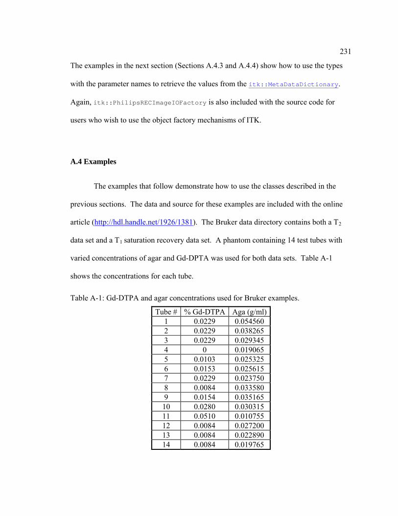
231

The examples in the next section (Sections A.4.3 and A.4.4) show how to use the t

with the parameter names to retrieve the values from the

ypes

itk::MetaDataDictionary.

Again,

itk::PhilipsRECImageIOFactory is also included with the source code for

users who wish to use the object factory mechanisms of ITK.

A.4 Examples

The examples that follow demonstrate how to use the classes described in the

previous sections. The data and source for these examples are included with the online

article (http://hdl.handle.net/1926/1381). The Bruker data directory contains both a T2

data set and a T1 saturation recovery data set. A phantom containing 14 test tubes with

agar and Gd-DPTA was used for both data sets. Table A-1 varied concentrations of

shows the concentrations for each tube.

Table A-1: Gd-DTPA and agar concentrations used for Bruker examples.

Tube # % Gd-DTPA Aga (g/ml)1 0.0229 0.054560 2 0.0229 0.038265 3 0.0229 0.029345 4 0 0.019065 5 0.0103 0.025325 6 0.0153 0.025615 7 0.0229 0.023750 8 0.0084 0.033580 9 0.0154 0.035165 10 0.0280 0.030315 11 0.0510 0.010755 12 0.0084 0.027200 13 0.0084 0.022890 14 0.0084 0.019765



232

Two separate phantoms were used for the Philips T and T1 examples. The

-2 (g/ml) concentration

-2

on a 3.0 T Bruker MedSpec MR system. The TR time was 1595.03

B021304.oj1/3/pdata/1/ folder. The source code is located in the

381

2

phantom for the T2 example was designed to mimic brain white matter (WM) and gray

matter (GM). A cylindrical container was filled with 2:6224×10

agar doped with 0.024% Gd-DTPA (white matter) and embedded within the container

were 17 plastic spheres filled with 1:8382×10 (g/ml) agar doped with 0.007% Gd-

DTPA (gray matter). The T1 phantom contains 5 tubes with varying amounts of Gd-

DTPA. Table A-2 shows the concentration of Gd-DTPA for each numbered tube.

Table A-2: Gd-DTPA concentrations for phantom used in Philips T1 example.

Tube # % Gd-DTPA1 0.043 2 0.024 3 0.014 4 0.008 5 0

A.4.1 Bruker 2DSEQ T parameter map 2

In this example a T2 parameter map is generated using a multi-echo spin-echo

sequence acquired

ms and 11 echo images were acquired with a starting TE of 7.919 ms and an echo spacing

of 7.919 ms (final echo time was 87.107 ms). A single 3 mm slice was acquired with a

256 x 256 matrix size and 20 cm x 20 cm field of view (FOV). The data for this example

is located in the DC

BrukerT2Map.cxx file (both available online http://hdl.handle.net/1926/1 ).


233

BrukerT2Map.cxx takes up to 9 arguments. The first 5 arguments are required

he input Bruker 2dseq, the output T2 parameter

constant (S0) map filename, the output constant

-squared map filename. The remaining 4 optional

R2

gorithm to use (default is LINEAR), the maximum T2 time (default

t image (default is 0).

output T2), 0 (use LINEAR

2 time of 2.0 seconds), and 1000 (every voxel less

rect number of arguments and reading the arguments

tion:

if( !imageIO->CanReadFile(inputFilename) )

"Could not read 2dseq file" << std::endl; return 1; }

mation.

ation();

and are used to specify the full path of t

map filename, the output exponential

map (C) filename, and the output R

arguments are used to control the output, specifically whether or not to output T2 or

(default is T2), the al

is 10 seconds), and a baseline threshold value for masking the inpu

The optional parameters used for this example are 0 (

algorithm Eq. A.5), 2.0 (maximum T

than 1000 set to zero).

After checking for the cor

from the command line, the program attempts to read the Bruker 2dseq and get the image

informa

// Create 2DSEQ reader and check the file if it can be read. Bruker2DSEQImageIOType::Pointer imageIO = Bruker2DSEQImageIOType::New();

{ std::cerr <<

// Read the image infor imageIO->SetFileName(inputFilename); try { imageIO->ReadImageInform }

ExceptionObject &err ) catch( itk:: {

::cerr << "ExceptionObject caught"; std std::cerr << " : " << err.GetDescription(); return 1; }

234 If the image is read without errors, the program will attempt to get the echo times from

the itk::MetaDataDictionary:

// Get the echo times in ms. Bruker2DSEQImageIOType::ACQEchoTimeContainerType::Pointer ptrToEchoes = NULL; if(!itk::Expo

uker2DSEQseMetaData< ImageIOType::ACQEchoTimeContainerType::Pointer>

geIO->GetMetaDataDictionary(),itk::ACQ_ECHO_TIME,ptrToEchoes))

return 1;

dictionary"

} unsigned int numberOfEchoTimes = ptrToEchoes->Size();

E times, typically a multi-

cquired using a

,

pulse across a sample

herefore in order to

t.

conds:

i++)

onvert to seconds

Br (ima

{ std::cerr << "Could not get the echo times" << std::endl;

} if( !ptrToEchoes ) { std::cerr << "Received NULL echo times pointer from meta

<< std::endl; return 1;

Instead of acquiring multiple spin-echo images with different T

echo spin-echo image is acquired to measure T2. A spin-echo image is a

90 degree RF pulse followed by a 180 degree RF pulse. To acquire a multi-echo data set

a series of 180 degree RF pulses follow the first 90 and 180 degree pulses (see Chapter 2

Section 2.2.2). The application of a perfectly homogenous 180 RF

is difficult and imperfections in the flip-angle lead to what are called stimulated echoes

for the echo images acquired after the first 180 degree RF pulse. T

measure T the first echo image without the stimulated echo signal is usually thrown ou2

The following for loop below will do that as well as convert the echo times to se

for(unsigned int i=1; i<(unsigned int)numberOfEchoTimes; { // c


235 ptrToEchoes->SetElement(i-1,ptrToEchoes->ElementAt(i)/1000.0f);

rOfEchoTimes;

is limited to reading

ment

ill convert the 3D image to an itk::VectorImage

} ptrToEchoes->CastToSTLContainer().pop_back(); --numbe if( numberOfEchoTimes < 2 ) { std::cerr << "Must have at least 2 echo images to calculate T2" <<std::endl; return 1; } As already mentioned previously, itk::Bruker2DSEQImageIO

Bruker 2dseq images in 3D only. For a multi-echo spin-echo image, the 2dseq is in

reality a 4D image with the fourth dimension being the echo time. The code seg

below w , which will be supplied as an

itk::MRT2ParameterMap3DImageFilter

same time. EchoTimes+1);

VectorImageType::RegionType region; VectorImageType::SizeType size; size[0] = dims[0]; size[1] = dims[1]; size[2] = realSlices; VectorImageType::IndexType index; index[0] = 0; index[1] = 0; index[2] = 0; region.SetSize(size); region.SetIndex(index); VectorImageType::Pointer vectorImage = VectorImageType::New(); vectorImage->SetRegions(region); vectorImage->SetVectorLength(numberOfEchoTimes); VectorImageType::PointType origin = baselineReader->GetOutput()-

ge->SetSpacing(baselineReader->GetOutput()->GetSpacing()); vectorImage->SetDirection(baselineReader->GetOutput()->GetDirection()); vectorImage->Allocate(); ImageType::IndexType echoIndex;

input to :

// Get real number of slices and create vector image. // Also threshold the image at the int realSlices = dims[2]/(numberOf

>GetOrigin(); origin[2] = -baselineReader->GetOutput()->GetSpacing()[2]*size[2]/2.0f; vectorImage->SetOrigin(origin); vectorIma


236 for(index[0]=0,echoIndex[0]=0;index[0]<(int)size[0];index[0]++,echoIndex[0]++) { for(in 0 0; n index[1]++,echoIndex[1]++) { for(ind [2] n dex { // Multi-echo Bruker images are stored as they are acquired. This // means that the images are not stored as volumes. We need to ut // each echo from each slice into the vector as follows: echoIndex[2] = index[2]*(numberOfEchoTimes+1) + 1;

= baselineReader->GetOutput()->GetPixel(echoIndex); elVal;

vectorImage->SetPixel(index, echoVector); }

dex[1]= ,echoIndex[1]= index[1]<(i t)size[1];

ex =0;index[2]<(i t)size[2];in [2]++)

p

// Skip to next slice ignoring the first echo.

VectorImageType::PixelType echoVector(numberOfEchoTimes); for(unsigned int echo=0; echo<numberOfEchoTimes; echo++) { ImageType::PixelType pixelVal

echoVector[echo] = (pixelVal < threshold)?0:pix ++echoIndex[2]; }

} } The fitting options and itk::VectorImage input data are input into

itk::MRT2ParameterMap3DImageFilter as follows:

// Create T2 mapping class. MRT2 = MRT2ParameterMap3DImageFilterType::New();

{

t2Map->SetAlgorithm(MRT2ParameterMap3DImageFilterType::NON_LINEAR);

case MRT2ParameterMap3DImageFilterType::NON_LINEAR_WITH_CONSTANT:

std::cerr << "In valid algorithm = " << algorithm << std::endl;

ParameterMap3DImageFilterType::Pointer t2Map

// Select the fit type. switch(algorithm)

case MRT2ParameterMap3DImageFilterType::LINEAR: t2Map->SetAlgorithm(MRT2ParameterMap3DImageFilterType::LINEAR); break; case MRT2ParameterMap3DImageFilterType::NON_LINEAR:

break;

t2Map->SetAlgorithm( MRT2ParameterMap3DImageFilterType::NON_LINEAR_WITH_CONSTANT); break; default:


237 return 1; } t2Map->SetMaxT2Time(maxT2Time); t2Map->SetMREchoImage(ptrToEchoes, vectorImage); if( r2Mapping )

{

} #ifdef

Finally

t2Map->PerformR2MappingOn();

NO_MULTI_THREADING t2Map->SetNumberOfThreads(1); #endif

, the itk::VectorImage output is connected to the input of

itk::VectorIndexSelectionCastImageFilter so that the extracted components may

ten to file with the file names supplied on tbe writ he command line:

// E VectorIndexSelectionCastImageFilterType::Pointer extractComp =

xtr Writ

-squared output images for this

exampl

xtract each output component and write to disk.

VectorIndexSelectionCastImageFilterType::New(); e actComp->SetInput(t2Map->GetOutput());

erType::Pointer writer = WriterType::New(); writer->SetInput(extractComp->GetOutput());

Figure A-1 shows the T2, exponent constant, and R

e and Table A-3 contains the average T2 time, exponent constant, and R-squared

value for each tube.


http://www.itk.org/Doxygen/html/classitk_1_1VectorIndexSelectionCastImageFilter.html

238

Figur A-1: Output from Bruker Te T2 par the R-squared A-1 are labeled in red on the T2 paramete

2 parameter map example. The image on the left is the ameter map, the middle image is the constant S0, and the right image is map. The tube numbers from Table r

To verify the fitted values, the magnitude of the image intensity at the center of tube 1

was plotted for each echo image as a function of echo time and the fitted function was

ap image. Note that some contrast exists amongst the tubes in the constant image S0.

This indicates that the TR of 1595.03 ms was not long enough to remove thecontributions due to T1 in Eq. A.1.

Table A-3: Average T2, S0, and R-squared value for each tube in the Bruker T2 phantom example.

Tube # Average T2 (ms) Average S0 Average R-squared

m

1 38.147 ± 0.982 23567 ± 594 0.783 ± 0.002 2 50.697 ± 1.088 25385 ±690 0.799 ± 0.001 3 62.540 ± 1.344 25083 ± 459 0.807 ± 0.001 4 99.065 ± 2.733 16889 ± 395 0.818 ± 0.001 5 74.704 ± 1.548 21102 ± 520 0.812 ± 0.001 6 72.822 ± 1.442 23036 ± 454 0.811 ± 0.001 7 75.776 ± 2.633 24721 ± 2778 0.812 ± 0.002 8 59.594 ±1.511 20244 ± 513 0.804 ± 0.001 9 55.987 ± 1.256 23424 ± 613 0.802 ± 0.001 10 61.708 ± 1.233 26303 ± 693 0.806 ± 0.001 11 129.920 ± 4.652 31113 ± 1307 0.823 ± 0.001 12 71.762 ± 1.579 20737 ± 475 0.810 ± 0.001 13 81.658 ± 2.013 21333 ± 532 0.814 ± 0.001 14 93.423 ± 2.056 21607 ± 471 0.817 ± 0.000

239

added as an overlay in Figure A-2 . As can be seen in the figure, the fitted values match

the plotted MR signal values very wel

ages

d 10000

l.

Figure A-2: A plot of image intensity (Si) as a function of TE for a pixel in the center of lly, the fitted curve matches the experimental tube 1 with overlay of fitted curve. Visua

data very well.

A.4.2 Bruker 2DSEQ T1 parameter map

This example calculates a T1 parameter map using the saturation recovery method

acquired on a 3.0 T Bruker MedSpec MR system. The TE time was 10 ms and 11 im

were acquired with TR = 30, 50, 100, 200, 500, 1000, 2000, 3000, 4000, 6000, an

ms. The single slice acquisition thickness was 10 mm. The matrix size was 128 x 128

240

and the FOV 20 cm x 20 cm. The data for this example is located in the

DCB021304.oj1/5/pdata/1/ folder. The source code is located in the BrukerT1Map.cxx

://hdl.handle.net/1926/1381file (both available online http ).

BrukerT1Map.cxx are essentially the same as

n A.4.1). The optional parameters used for this example are 0

DY_STATE_3PARAM algorithm Eq. A.8), 5.0

d 20546109 (every voxel less than 20546109 set to

r the correct number of arguments and reading the arguments

ommand line, the program attempts to read the Bruker 2dseq and get the image

s in BrukerT2Map.cxx (Section A.4.1). After successfully

epetition times or the

t algorithm specified on the command line and

imes depending on the algorithm. tionTimeContainerType::Pointer

STEADY_STATE) ||

_STEADY_STATE_3PARAM))

turation recovery fit type. taData< eIOType::ACQRepetitionTimeContainerType::Pointer> aDataDictionary(),itk::ACQ_REPETITION_TIME, )

"Could not get the repetition times" << std::endl;

The arguments to

BrukerT2Map.cxx (Sectio

(output T ), 5 (use HYBRID1 _STEA

(maximum T1 time of 5.0 seconds), an

zero).

After checking fo

from the c

information - the same a

reading the image information the program will extract the r

inversion times depending on the fi

convert the times to seconds:

// Extract repetition/inversion tBruker2DSEQImageIOType::ACQRepeti

ptrToTimePoints = NULL;

if((algorithm == T1ParameterMap3DImageFilterType::IDEAL_MR

(algorithm == T1ParameterMap3DImageFilterType::HYBRIDMR

{ // Repetition times for the sa

if(!itk::ExposeMe Bruker2DSEQImag

(imageIO->GetMet ptrToTimePoints)

{ std::cerr <<

return 1; }


241 } else

// Inversion times for all others.

e::ACQRepetitionTimeContainerType::Pointer>

etMetaDataDictionary(),itk::ACQ_INVERSION_TIME,ptrToTimePoints))

std::cerr << "Could not get the inversion times" << std::endl;

if( !ptrToTimePoints )

std::cerr << "Received NULL repetition/inversion times pointer";

}

at least 2 images to calculate T1" <<

}

times to seconds. for(unsigned int i=0; i<(unsigned int)numberOfTimePoints; i++)

onds ptrToTimePoints->SetElement(i,ptrToTimePoints-

}

read and then an itk::VectorImage

{ if(!itk::ExposeMetaData< Bruker2DSEQImageIOTyp (imageIO->G { return 1; } } { std::cerr << " from meta dictionary" << std::endl; return 1; unsigned int numberOfTimePoints = ptrToTimePoints->Size(); if( numberOfTimePoints < 2 )

{ std::cerr << "Must have d::endl; st

return 1; // Convert the { // convert to sec >ElementAt(i)/1000.0f); If this task completes without errors, the image is

tead of thresholding the entire data series using the

esholded and used as a

e itk::VectorImage

is created to store the data series. Ins

threshold value, just the first image volume in the series is thr

mask when the data is copied to th :

slices and create vector image. same time. mePoints;

ze[2] = realSlices;

// Get real number of // Also threshold the image at the

Ti int realSlices = dims[2]/numberOf VectorImageType::RegionType region; VectorImageType::SizeType size; size[0] = dims[0];

ize[1] = dims[1]; s si



242 VectorImageType::IndexType index;

index[1] = 0; index[2] = 0; region.SetSize(size);

ex);

vectorImage->SetRegions(region);

etSpacing()); (baselineReader->GetOutput()-

ype::IndexType imageTimePointIndex;

]=0;index[1]<(int)size[1];

stored as they

if((algorithm != erType::IDEAL_STEADY_STATE) &&

Y_STATE_3PARAM))

ePoints;

or(numberOfTimePoints); numberOfTimePoints;

aturation recovery

le filling the

EADY_STATE)

index[0] = 0;

region.SetIndex(ind VectorImageType::Pointer vectorImage = VectorImageType::New();

vectorImage->SetVectorLength(numberOfTimePoints); VectorImageType::PointType origin = baselineReader->GetOutput()->GetOrigin();

rigin[2] = -baselineReader->GetOutput()- o>GetSpacing()[2]*size[2]/2.0f; vectorImage->SetOrigin(origin);

baselineReader->GetOutput()->G vectorImage->SetSpacing(vectorImage->SetDirection

>GetDirection()); vectorImage->Allocate();

ageT Im imageTimePointIndex.Fill(0); for(index[0]=0,imageTimePointIndex[0]=0;index[0]<(int)size[0]; index[0]++,imageTimePointIndex[0]++) {

for(index[1]=0,imageTimePointIndex[1 index[1]++,imageTimePointIndex[1]++) { for(index[2]=0;index[2]<(int)size[2];index[2]++ ) {

// Multi-echo inversion recovery Bruker images are are

s // acquired. This means that the images are not stored avolumes. We // need to put each echo from each slice into the vector as

ows: foll

MRT1ParameterMap3DImageFilt (algorithm !=

HYBRID_STEADMRT1ParameterMap3DImageFilterType:: { // Skip to next slice

x[2]*numberOfTim imageTimePointIndex[2] = inde } VectorImageType::PixelType timePointVect

timePoint< for(unsigned int timePoint=0; timePoint++) {

lumes in the s // Images are stored as vocase, so we

on whi // need to skip to each new repetitivector. if((algorithm ==

:IDEAL_STMRT1ParameterMap3DImageFilterType: || (algorithm ==

243 MRT1ParameterMap3DImageFilterType::HYBRID_STEADY_STATE_3PARAM) )

ntIndex[2] = index[2] + (realSlices*timePoint); }

Type::PixelType pixelVal = baselineReader->GetOutput()->GetPixel(imageTimePointIndex); ImageType::PixelType maskVal = 0;

1ParameterMap3DImageFilterType::IDEAL_STEADY_STATE) || (algorithm ==

TATE_3PARAM))

index); }

dexType tempIndex = index; = tempIndex[2]*numberOfTimePoints; // Skip to

maskVal = t1Mask->GetOutput()->GetPixel(tempIndex);

kVal==0)?0:pixelVal; if((algorithm !=

terMap3DImageFilterType::IDEAL_STEADY_STATE)

T1ParameterMap3DImageFilterType::HYBRID_STEADY_STATE_3PARAM) ) {

ointIndex[2]; }

mePointVector);

e - the

1,

ared

{ imageTimePoi Image if((algorithm == MRT MRT1ParameterMap3DImageFilterType::HYBRID_STEADY_S { maskVal = t1Mask->GetOutput()->GetPixel( else { VectorImageType::In tempIndex[2]xt slice ne

} timePointVector[timePoint] = (mas MRT1Parame && (algorithm != MR ++imageTimeP } vectorImage->SetPixel(index, ti } } } Finally, the T map is calculated, the components extracted, and then written to fil1

same as in the Bruker T2 map example (Section A.4.1). Figure A-3 shows the T

exponent constant (S0), constant (B), and R-squared output images for this example and

Table A-4 contains the average T1 time, exponent constant, constant, and R-squ

value for each tube.

244

Figure A-3: Output from Bruker T1 parameter map example. The image on the top left isage is the

umbers from little hort

the T parameter map, the top1 middle image is the constant S0, the top right imp. The tube nconstant B, and the bottom middle image is the R-squared ma

Table A-1 are labeled red on the T1 parameter map image. Unlike Figure A-1 very s was scontrast exists in the constant image S0. This indicates that the TE of 10 m

enough to remove the contributions due to T2 in Eq. A.1.

245

verify the fitted values, the magnitude of the MR signal at the center of tube 1 was

tion of repetition time and the fitted function

4. Again, as can be seen in the figure, the fitted

age intensity values very well.

rukeTable A-4: Average T1, S0, constant B, and R-squared value for each tube in the B r T1 phantom example.

Tube # Average T1 (ms) Average S0 Average B Average R-squared1 825.51 ± 9.00 1.3027 × 10 ± 6.3788 × 109 7 1.0438 ± 0.0017 0.999 ± 0.000

2 838.20 ± 6.65 1.5196 × 109 ± 4.5192 × 107 1.0487 ± 0.0014 0.998 ± 0.000

3 825.85 ± 15.32 1.4088 × 109 ± 6.9022 × 107 1.0596 ± 0.0024 0.998 ± 0.000

4 1908.40 ± 22.33 1.4908 × 109 ± 7.9244 × 107 1.0538 ± 0.0025 0.996 ± 0.000

5 1186.40 ± 14.60 1.4531 × 109 ± 5.9687 × 107 1.0571 ± 0.0028 0.998 ± 0.000

6 1019.90± 9.41 1.4596 × 109 ± 6.4035 × 107 1.0586 ± 0.0025 0.998 ± 0.000

1.4719 × 109 ± 5.0358 × 107 1.0653 ± 0.0026 0.998 ± 0.000 7 838.67 ± 11.49

8 1260.90 ± 15.10 1.4911 × 10 ± 6.9226 × 9 107 1.0481 ± 0.0023 0.998 ± 0.000

9 999.66 ± 8.06 1.4871 × 109 ± 6.2972 × 107 1.0491 ± 0.0021 0.998 ± 0.000

10 734.15 ± 7.62 1.4678 × 109 ± 6.6556 × 107 1.0601 ± 0.0028 0.998 ± 0.000

1.6377 × 109 ± 2.4449 × 108 1.1015 ± 0.0075 0.999 ± 0.000 11 532.28 ± 12.63

154 × 109 ± 7.2595 × 107 1.0515 ± 0.0023 0.998 ± 0.000 12 1275.90 ± 13.15 1.5

13 1310.00 ± 10.64 1.6134 × 109 ± 6.2195 × 107 1.0526 ± 0.0021 0.998 ± 0.000

14 1317.20 ± 13.43 1.6257 × 109 ± 6.8480 × 107 1.0567 ± 0.0017 0.998 ± 0.000

To

plotted for each image repetition as a func

was added as an overlay in Figure A-

values match the plotted MR im

246

Figure A-4: A plot of image intensity (Si) as a function of TR for a pixel in the center of h overlay of fitted curve. Again, this demonstrates that the predicted data is a

or the experimental data. tube 1 witgood fit f

A.4.3 Philips REC T2 parameter map

tions A.4.1 and A.4.2) used the Bruker data to

T2 and T1 parameter maps. In this example a Philips multi-echo spin-echo

.PAR and

ed in PhilipsT2Map.cxx (both available online

81

The previous examples (Sec

generate

PAR/REC data set is used to calculate T2. The name of the file is T2_Map_4_3

the example code is sav

http://hdl.handle.net/1926/13 ). The image was acquired on a 3.0 T Philips Achieva

ce with SENSE factor 2.5, 256 x 256 matrix size, 230 system. A single 4 mm axial sli


247

mm x 230 mm FOV, TE of 252.901 ms, and 14 echoes (TE 8, 16, 24, 32, 40, 48, 56, 64,

901 ms TR time is not ideal for

rall

deal for testing the non-linear

itk::MRT2ParameterMap3DImageFilter used in this example.

ents as BrukerT2Map.cxx (Section

ss than 14 set to zero).

ake sure that the number of

choTimes = 0; tempNum = 0;

f echoes. ExposeMetaData<int>(imageIO->GetMetaDataDictionary(), _MaxNumberOfEchoes,tempNum) )

{ f echoes" <<

umberOfEchoTimes = static_cast<unsigned int>(tempNum);

at st numberOfEchoTimes image

e to have more if the than one image type

s(1); s(2);

imensions(3); ( numberOfEchoTimes > (unsigned int)dims[3] )

72, 80, 88, 96, 104, and 112 ms) was acquired. The 252.

measuring T2, as it will include significant T1 contributions and will reduce the ove

signal to noise ratio (SNR) of the image. However, this is i

fitting capabilities of

PhilipsT2Map.cxx takes the same 9 argum

A.4.1). For this example the optional parameters are 0 (output T2), 1 (use

NON_LINEAR algorithm Eq. A.5), 2.0 (maximum T2 time of 2.0 seconds), and 14

(every voxel le

After successfully reading the image information using

itk::PhilipsRECImageIO, PhilipsT2Map.cxx checks to m

image volumes is greater than or equal to the number of echo times:

intunsigned int numberOfE

// Make sure that the number of images // stored in the REC file matches the number o

if( !itk:: itk::PAR

std::cerr << "Could not determine the number od::endl; st

return 1; } n

// Get the image dimensions and make sure th

// there exists at lea // volumes. It's possibl

EC file contains more // R // (i.e. magnitude, phase, real, imaginary, etc.)

[0] = imageIO->GetDimensions(0); dims dims[1] = imageIO->GetDimension

Dimension dims[2] = imageIO->Getdims[3] = imageIO->GetD if

248 { std::cerr << "The number of echoes is larger than the number of

< std::endl; urn 1;

ble that more than one image type is stored in the

the image used in this example contains both the magnitude and

lices

eIO will automatically sort the slices by image type

.

ntains the magnitude image using the

image "; std::cerr << "blocks" < ret } As noted in the code comments it's possi

REC file. For example

phase images, so instead of . By default REC files store the sdims[3] = 28 14

unsorted. itk::PhilipsRECImag

when the data is read. However, in order to calculate T , the magnitude image is needed2

The following code checks to see if the REC file co

itk::MetaDataDictionary:

// Check to see if the REC file has at least the magnitudehaveMagnitude = 0;

image.

e imageTypes;

itk::PAR_NumberOfImageTypes,numberOfImageTypes) )

image types" <<

Type> mageTypes)

the image types vector" << std::endl;

int int numberOfImageTypes = 0;

TypesTyp PhilipsRECImageIOType::Imageif( !itk::ExposeMetaData<int>(imageIO->GetMetaDataDictionary(),

{ std::cerr << "Could not determine the number of

std::endl; return 1; } if( !itk::ExposeMetaData<PhilipsRECImageIOType::ImageTypes

mageIO->GetMetaDataDictionary(), itk::PAR_ImageTypes,i (i) { std::cerr << "Could not get

return 1; } for(int j=0; j<numberOfImageTypes; j++)

{ j] == 0 ) if( imageTypes[

{ haveMagnitude = 1;

} } if( !haveMagnitude ) {


249 std::cerr << "Magnitude image type not found in REC file" <<

that must be dealt with when using Philips PAR/REC image data is the

s. The Philips T1 example (Section A.4.4) makes

of this feature to extract the phase corrected real image for calculating T1 via the

re than 1 scanning sequence exists in

r:

one scanning sequence, the T2 map cannot be processed.

= 0; imageIO->GetMetaDataDictionary(),

ine the number of scanning

::cerr << std::endl;

1 )

t process a T2 map when the number of scanning"; is greater than 1" << std::endl;

6 bit signed integers. The PAR file lists rescale

S), and scale slope (SS) values for converting the integer

ting

std::endl; return 1; } An issue

existence of multiple scanning sequence

use

inversion recovery method. However, for T2, if mo

the REC file, processing is aborted with an erro

make sure that there is only // Check to therwise // o

int numberOfScanningSequences !itk::ExposeMetaData<int>( if(

itk::PAR_NumberOfScanningSequences,numberOfScanningSequences) ) {

<< "Could not determ std::cerr ces"; sequen

std return 1; }

> if( numberOfScanningSequences {

d::cerr << "Canno st std::cerr << " sequences

turn 1; re } Philips REC images are stored as 1

intercept (RI), rescale slope (R

data back to the original floating point data. As described in the PAR file, the floa

point value is obtained using Eq. A.15:

SSRSRIRSPV *FP

*+

= A.15

250

where PV is the pixel value in the REC file and FP is the floating point value. The

cale values using the following source demonstrates how to get the s

itk::MetaDataDictionary and convert the image to floating point using

itk::ShiftScaleImageFilter and itk::ShiftScaleInPlaceImageFilter:

e 16 bit image to floating

ScanningSequenceImageTypeRescaleValuesContainerT

TypeRescaleValues = NULL; OType sContainerType::Pointer>

leValues,

;

scanning sequence/image types vector"; td::endl;

rType::Pointer

alueVector )

ge to floating point value. nly = NULL; shiftAndScale = NULL;

TypeRescaleValuesType rescaleValues = tAt(0); // Magnitude image is the first

0) && // scale slope (SS) aleValues[1] != 0) ) // rescale slope (RS)

leImageFilterType::New();

// Get rescale values for converting thpoint.

eIOType::PhilipsRECImagype ::Pointer scanSequenceImage if( !itk::ExposeMetaData<PhilipsRECImageI ::ScanningSequenceImageTypeRescaleValue (imageIO->GetMetaDataDictionary(), itk::PAR_ScanningSequenceImageTypeResca

RescaleValues) ) scanSequenceImageType { std::cerr << "Could not get the rescale values for each scanning" std::cerr << " sequence and image type" << std::endl; return 1; } if( !scanSequenceImageTypeRescaleValues ) { std::cerr << "Received NULL std::cerr << " pointer from meta dictionary" << s return 1; }

ipsRECImageIOType::ImageTypeRescaleValuesContaine Phil rescaleValueVector = scanSequenceImageTypeRescaleValues->ElementAt(0); //Only 1 scanning sequence.

!rescaleV if( { std::cerr << "Received NULL rescale values vector pointer from";

d::cerr << " meta dictionary" << std::endl; st return 1; }

hange ima // C ShiftScaleImageFilterType::Pointer scaleO

tScaleInPlaceImageFilterType::Pointer Shif PhilipsRECImageIOType::Image

aleValueVector->Elemen rescelement.

escaleValues[2] != if( (resc (r

{ scaleOnly = ShiftSca


http://www.itk.org/Doxygen/html/classitk_1_1ShiftScaleImageFilter.html

http://www.itk.org/Doxygen/html/classitk_1_1ShiftScaleInPlaceImageFilter.html

251 scaleOnly->SetInput(t2Mask->GetOutput());

leInPlaceImageFilterType::New(); le->SetInput(scaleOnly->GetOutput());

ftAndScale->SetShift(rescaleValues[0]); //rescale intercept (RI)

s data is 4D, it is easier in this instance to use AddMREchoImage() to

ap3DImageFilter instead of

scaleOnly->SetScale(rescaleValues[1]); //RS shiftAndScale = ShiftSca shiftAndSca shi shiftAndScale->SetScale(1.0/(rescaleValues[2]*rescaleValues[1])); //1/(SS*RS) } else { std::cerr << "Invalid rescale values" << std::endl; return 1; } Because the Philip

add the input images to itk::MRT2ParameterM

SetMREchoImage(). This is done using an itk::VectorContainer of

itk::ExtractImageFilter smart pointers, one for each echo image, to extract the

:New();

ype extractionSize;

e[3] = 0; extractionIndex;

geIOType::EchoTimesContainerType::Pointer ptrToEchoes =

pe::

ionary(), itk::PAR_EchoTimes,ptrToEchoes)

ptrToEchoes )

images from the 4D volume as follows:

ExtractImageFilterContainerType::Pointer extractVOI = ageFilterContainerType: ExtractIm

extractVOI->resize(numberOfEchoTimes-1); ExtractImageFilterType::InputImageRegionType extractionRegion;

actImageFilterType::InputImageSizeT Extr extractionSize[0] = dims[0]; extractionSize[1] = dims[1];

ze[2] = dims[2]; extractionSiactionSiz extr

ExtractImageFilterType::InputImageIndexTypeactionIndex[0] = 0; extr

extractionIndex[1] = 0; extractionIndex[2] = 0;

gion.SetSize(extractionSize); extractionReipsRECIma Phil

NULL; if(!itk::ExposeMetaData<PhilipsRECImageIOType::EchoTimesContainerTyPointer> (imageIO->GetMetaDataDict) { std::cerr << "Could not get the echo times" << std::endl; return 1; } if( !

http://www.itk.org/Doxygen/html/classitk_1_1VectorContainer.html

http://www.itk.org/Doxygen/html/classitk_1_1ExtractImageFilter.html

252 { std::cerr << "Received NULL echo times pointer from"; std::cerr << " meta dictionary" << std::endl; return 1; } if( ptrToEchoes->size() != numberOfEchoTimes )

vector does"; ::cerr << " not match the number of echoes listed in";

std::cerr << " the PAR file" << std::endl;

oTimes; i++)

Type::New()); ftAndScale->GetOutput());

);

Like the Bruker T2 example (Section A.4.1), the first echo image is not used and the echo

times are converted to seconds. Figure A-5 shows th images from this example.

Figure A-6 plots the fitted data against the experimentally acquired data points for a

location at the center of a gray matter region in the phantom. As seen in the figure, the

nonlinear fitting routine found a reasonable fit in spite of t

{ std::cerr << "The size of the echo times std return 1; } for(unsigned int i=1; i<numberOfEch { extractVOI->SetElement(i-1, ExtractImageFilter

extractVOI->ElementAt(i-1)->SetInput(shi extractionIndex[3] = i; extractionRegion.SetIndex(extractionIndex); extractVOI->ElementAt(i-1)->SetExtractionRegion(extractionRegion t2Map->AddMREchoImage(ptrToEchoes->ElementAt(i)/1000.0f, //convert to seconds extractVOI->ElementAt(i-1)->GetOutput()); }

e output

he noisy input data.

253

Figure A-5: Output from Philips T2 parameter map example. The image on the left is theT2 right image is the R-squared map. Like Figure A-1 significant T1 constant image S0 due to the extremely short TR of 252.901 ms.

parameter map, the middle image is the constant S0, and thecontrast exists in the

254

A.4.4 Philips REC T1 parameter map

The final example demonstrates an inversion recovery T1 parameter map

measurement using a fast inversion recovery Look-Locker sequence acquired on a 3.0 T

Philips Achieva system. The Philips T1 phantom specified at the beginning of this

section was used (Section A.4). The name of the file is T1_LL_10_1.PAR and the

example code is saved in PhilipsT1Map.cxx (both available online

Figure A-6: A plot of MR image intensity (Si) as a function of TE for a pixel in the center of the gray matter sphere used in the Philips T2 parameter map example with overlay of fitted curve. The exponential image intensity points are noisy due to the short TR 252.901 ms and SENSE factor 2.5. A reasonable fit was obtained in spite of the expected variation in the experimental data points.

255

http://hdl.handle.net/1926/1381). A single 2 mm axial slice with SENSE factor 2.5, 160

x 160 matrix size, 225 mm x 225 mm FOV, TR of 25.0 ms, TE of 4.45 ms, and 8

inversion times (TI 83, 532, 980,1429, 1877, 2325, 2774, and 3222 ms) was acquired.

PhilipsT1Map.cxx takes the same 9 parameters as BrukerT1Map.cxx (Section

A.4.2). For this example the optional parameters are 0 (output T1), 1 (use

INVERSION_RECOVERY algorithm Eq. A.9 ), 5.0 (maximum T1 time of 5.0 seconds),

and 50 (every voxel less than 50 set to zero). The IDEAL_STEADY_STATE, Eq. A.7,

and HYBRID_STEADY_STATE_3PARAM, Eq. A.8, algorithms are not supported.

r to the Philips T2 example (Section A.4.3), PhilipsT1Map.cxx

make sure that the number of image volumes is greater than or equal to the number of

time the number of time points in this case is equal to the number of

cardiac phases, instead of the number of echo times:

unsigned int numberOfTimePoints = 0; int tempNum = 0; // Find the maximum number of cardiac phases. if( !itk::ExposeMetaData<int>(imageIO->GetMetaDataDictionary(), itk::PAR_MaxNumberOfCardiacPhases,tempNum) ) std::cerr << "Could not determine the number of cardiac"; std::cerr << " phases" << std::endl; return 1; } numberOfTimePoints = static_cast if( numberOfTimePoints < 2 ) std::cerr << "Must have at least 2 cardiac phase images to"; std::cerr << " calculate T1" << std::endl; return 1; } and make sure that // there exists at least numberOfTimePoints image // volumes. It's possible to have more if the // REC file contains more than one image type // (i.e. magnitude, phase, real, imaginary, etc.)

Simila checks to

points. However,

{

<unsigned int>(tempNum);

{

// Get the image dimensions


256 dims[0] = imageIO->GetDimensions(0); dims[1] = imageIO->GetDimensions(1); dims[2] = imageIO->GetDimensions(2); { std::cerr << "The number of time points is larger than the number"; std::cerr << " of image blocks" << std::endl; return 1; } Unlike PhilipsT2Map.cxx, PhilipsT1Map.cxx requires either the magnitude image or

both the magnitude image and the phase corrected real image depending on the fit type.

The magnitude image is used to generate a binary mask using the optional threshold

value supplied on the command line. The phase corrected real image is listed as image

type 4 in the PAR file and is required for the non-absolute value inversion recovery

fitting options. The code below will check for the existence of the proper image types

stored in the itk::MetaDataDictionary and return with an error if the required image

type does not exist in the REC file:

// Check to see if we have the correct image types. int haveCorrectImage = 0; int numberOfImageTypes = 0; PhilipsRECImageIOType::ImageTypesType imageTypes; if( !itk::ExposeMetaData<int>(imageIO->GetMetaDataDictionary(), itk::PAR_NumberOfImageTypes,numberOfImageTypes) ) { std::cerr << "Could not determine the number of image types" << std::endl; return 1; } if( !itk::ExposeMetaData<PhilipsRECImageIOType::ImageTypesType> (imageIO->GetMetaDataDictionary(),itk::PAR_ImageTypes,imageTypes) ) { std::cerr << "Could not get the image types vector" << std::endl; return 1; } // Need image 4 (corrected real image) for inversion recovery/Look-Locker // fit type. if( (algorithm == MRT1ParameterMap3DImageFilterType::INVERSION_RECOVERY) ||


257 (algorithm == MRT1ParameterMap3DImageFilterType::INVERSION_RECOVERY_3PARAM) || (algorithm == MRT1ParameterMap3DImageFilterType::LOOK_LOCKER) ) { for(int j=0; j<numberOfImageTypes; j++) { if( imageTypes[j] == 4 ) { haveCorrectImage = 1; } } if( !haveCorrectImage ) { o corrected real image type detected in PAR"; std::cerr << " file" << std::endl; return 1; } } // Now check for existence of the magnitude image. haveCorrectImage = 0; for(int j=0; j<numberOfImageTypes; j++) { if( imageTypes[j] == 0 ) { haveCorrectImage = 1; } } if( !haveCorrectImage ) { ile" << std::endl; return 1; } If the correct image types exist in the REC file, as reported in the PAR file, the program

will attempt to read the inversion times from the itk::MetaDataDictionary

std::cerr << "N

std::cerr << "No magnitude image type detected in PAR f

. The

actual inversion times are listed as trigger times in the PAR file and are extracted as

follows:

ptrToTimePoints = NULL; if(!itk::ExposeMetaData< PhilipsRECImageIOType::TriggerTimesContainerType::Pointer> >GetMetaDataDictionary(),itk::PAR_TriggerTimes,ptrToTimePoints) ) {

// Get trigger times. PhilipsRECImageIOType::TriggerTimesContainerType::Pointer

(imageIO-


258 std::cerr << "Could not get the trigger times" << std::endl; return 1; } if( !ptrToTimePoints ) { std::cerr << "Received NULL trigger times pointer from meta"; std::cerr << " dictionary" << std::endl; return 1; } if( ptrToTimePoints->size() != numberOfTimePoints ) {

std::cerr << " number of cardiac phases listed in the PAR file" << std::endl; return 1; } After scaling the 16 bit data read using itk::PhilipsRECImageIO to floating point data

as detailed in the previous section (A.4.3), each 3D volume for each time point is

extracted, masked, and assigned as inputs to itk::MRT1ParameterMap3DImageFilter

using AddMRImage():

// Extract volumes according to algorithm type. if( (algorithm == MRT1ParameterMap3DImageFilterType::INVERSION_RECOVERY) || (algorithm == MRT1ParameterMap3DImageFilterType::INVERSION_RECOVERY_3PARAM) || (algorithm == MRT1ParameterMap3DImageFilterType::LOOK_LOCKER) ) { // Corrected real image is after the magnitude and real images in first // scanning sequence. for(unsigned int i=0; i<numberOfTimePoints; i++) { extractVOI->SetElement(i, ExtractImageFilterType::New()); extractVOI->ElementAt(i)->SetInput(shiftAndScale->GetOutput()); extractionIndex[3] = 2*numberOfTimePoints + i; extractionRegion.SetIndex(extractionIndex); extractVOI->ElementAt(i)->SetExtractionRegion(extractionRegion); maskFilterContainer->SetElement(i,MaskImageFilterType::New()); maskFilterContainer->ElementAt(i)->SetInput1( extractVOI->ElementAt(i)->GetOutput()); maskFilterContainer->ElementAt(i)->SetInput2(magnitudeMask->GetOutput()); // convert to seconds t1Map->AddMRImage(ptrToTimePoints->ElementAt(i)/1000.0f, maskFilterContainer->ElementAt(i)->GetOutput());

std::cerr << "The size of the time points vector does not match the";

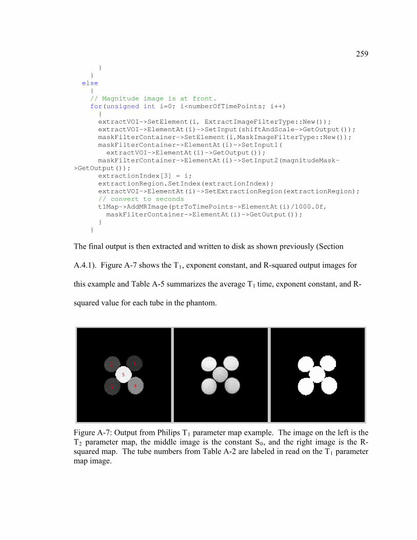
259 } } else { // Magnitude image is at front. for(unsigned int i=0; i<numberOfTimePoints; i++) { extractVOI->SetElement(i, ExtractImageFilterType::New()); extractVOI->ElementAt(i)->SetInput(shiftAndScale->GetOutput()); maskFilterContainer->SetElement(i,MaskImageFilterType::New()); maskFilterContainer->ElementAt(i)->SetInput1( extractVOI->ElementAt(i)->GetOutput()); maskFilterContainer->ElementAt(i)->SetInput2(magnitudeMask->GetOutput()); extractionIndex[3] = i; extractionRegion.SetIndex(extractionIndex); extractVOI->ElementAt(i)->SetExtractionRegion(extractionRegion); // convert to seconds t1Map->AddMRImage(ptrToTimePoints->ElementAt(i)/1000.0f, maskFilterContainer->ElementAt(i)->GetOutput()); } } The final output is then extracted and written to disk as shown previously (Section

A.4.1). Figure A-7 shows the T1, exponent constant, and R-squared output images for

this example and Table A-5 summarizes the average T1 time, exponent constant, and R-

squa .

red value for each tube in the phantom

Figure A-7: Output from Philips T1 parameter map example. The image on the left is theT2 parameter map, the middle image is the constant S0, and the right image is the R-squared map. The tube numbers from Table A-2 are labeled in read on the T1 parameter map image.

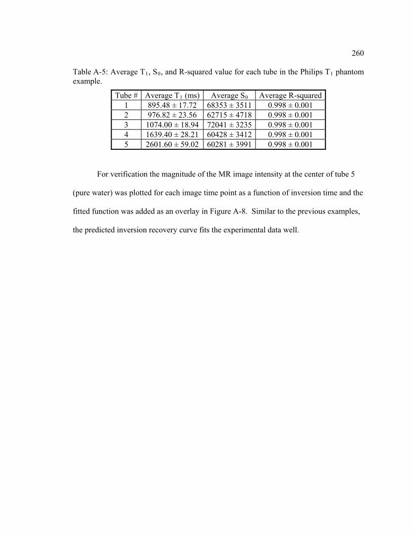
260

For verification the magnitude of the MR image intensity at the center of tube 5

(pure water) was plotted for each image time point as a function of inversion time and the

fitted function was added as an overlay in Figure A-8. Similar to the previous examples,

the predicted inversion recovery curve fits the experimental data well.

Table A-5: Average T1, S0, and R-squared value for each tube in the Philips T1 phantom example.

Tube # Average T1 (ms) Average S0 Average R-squared 1 895.48 ± 17.72 68353 ± 3511 0.998 ± 0.001 2 976.82 ± 23.56 62715 ± 4718 0.998 ± 0.001 3 1074.00 ± 18.94 72041 ± 3235 0.998 ± 0.001 4 1639.40 ± 28.21 60428 ± 3412 0.998 ± 0.001 5 2601.60 ± 59.02 60281 ± 3991 0.998 ± 0.001

261

A.5 Conclusion

This paper outlines the background, implementation, and use of a suite of classes

and programs for generating MR T2 and T1 parameter maps using Philips PAR/REC and

Bruker 2dseq image files. The supplied examples based on image phantoms demonstrate

that these classes generate valid parameter maps. Included with the MR parameter

mapping classes are new image readers for Philips PAR/REC and Bruker 2dseq image

Figure A-8: A plot of MR image intensity as a function of TI for a pixel in the center of tube 5 with overlay of fitted curve. Like the previous examples, this demonstrates that the predicted data is a good fit for the experimental data.

262

files, which are useful not only for MR parameter mapping, but also for integration with

DTI, segmentation, and registration pipelines within ITK.

A.6 References

[1] G. S. Pell, R. S. Briellmann, H. Pardoe, D. F. Abbott, and G. D. Jackson, "Composite voxel-based analysis of volume and T2 relaxometry in temporal lobe epilepsy," NeuroImage, vol. 39, pp. 1151-1161, 2008.

[2 tes, D. F. Abbott, and G. D. Jackson,

erop, J. Müller-Hübenthal, and T. Klockgether, "Voxel-based analysis of multiple-system atrophy of cerebellar type: complem tary results by combining voxel-based morphometry and voxel-based relaxometry," NeuroImage, vol. 25, pp. 287-293, 2005.

[4] D. C. Bigler, B.-Y. Lee, H. E. Stephens, C. M. Torok, J. R. Olson, J. Wang, K. R. Scott, Q. X. Yang, Z. Simmons, and M. B. Smith, "Multimodality Voxel-Based MRI Study - Possible Tool for Disease Diagnosis and Monitoring in ALS," in Proceedings 15th Scientific Meeting, International Society for Magnetic Resonance in Medicine, Berlin, Germany, 2007, p. 932.

[5] P. B. Kingsley, "Methods of measuring spin-lattice (T1) relaxation times: An annotated bibliography," Concepts in Magnetic Resonance, vol. 11, pp. 243-276, 1999.

[6] R. Deichmann, "Fast high-resolution T1 mapping of the human brain," Magnetic Resonance in Medicine, vol. 54, pp. 20-27, 2005.

[7] R. Deichmann and A. Haase, "Quantification of T1 values by SNAPSHOT-FLASH NMR imaging," Journal of Magnetic Resonance, vol. 96, pp. 608-612, 1992.

[8] R. Deichmann, D. Hahn, and A. Haase, "Fast T mapping on a whole-body pp. 206-209, 1999.

[9] P. A. Gowland and M. O. Leach, "Fast and accurate measurements of T-1 using a multi-readout single inversion-recovery sequence," Magnetic Resonance in Medicine, vol. 26, pp. 79-88, 1992.

[10] E. Henderson, G. McKinnon, T.-Y. Lee, and B. K. Rutt, "A fast 3D Look-Locker method for volumetric T1 mapping," Magnetic Resonance Imaging, vol. 17, pp. 1163-1171, 1999.

[11] A. M. Howseman, D. L. Thomas, G. S. Pell, S. R. Williams, and R. J. Ordidge, "Rapid T-1 mapping using interleaved echo planar imaging," Magnetic Resonance in Medicine, vol. 41, pp. 368-374, 1999.

] G. S. Pell, R. S. Briellmann, A. B. Wai"Voxel-based relaxometry: a new approach for analysis of T2 relaxometry changes in epilepsy," NeuroImage, vol. 21, pp. 707-713, 2004.

[3] K. Specht, M. Minnen

1scanner," Magnetic Resonance in Medicine, vol. 42,

263

[12] for mapping the longitudinal e, vol. 181, pp. 98-106, 2006.

[13] D. C. Look and D. R. Locker, "Time Saving in Measurement of NMR and EPR Relaxation Times," Review of Scientific Instruments, vol. 41, pp. 250-251, 1970.

[14] au, S. J. Riederer, I. Anno, and Y. Itai, "Rapid T1 estimation using tagged magnetization-prepared gradient-echo MR imaging," Magnetic Resonance in Medicine, vol. 26, pp. 377-385, 1992.

[15] N. J. Shah, M. Zaitsev, S. Steinhoff, and K. Zilles, "A New Method for Fast Multislice T1 Mapping," NeuroImage, vol. 14, pp. 1175-1185, 2001.

[16] S. Steinhoff, M. Zaitsev, K. Zilles, and N. J. Shah, "Fast T1 mapping with volume coverage," Magnetic Resonance in Medicine, vol. 46, pp. 131-140, 2001.

[17] C. Y. Tong and F. S. Prato, "A novel fast T1-mapping method," Journal of Magnetic Resonance Imaging, vol. 4, pp. 701-708, 1994.

[18] D. C. Zhu and R. D. Penn, "Full-brain T1 mapping through inversion recovery Magnetic Resonance in

[19] C. Zuoqun, F. S. Prato, and C. McKenzie, "T1 fast acquisition relaxation mapping (T1-FARM): an optimized reconstruction," IEEE Transactions on Medical Imaging, vol. 17, pp. 155-160, 1998.

J.-J. Hsu and G. H. Glover, "Rapid MRI methodrelaxation time," Journal of Magnetic Resonanc

M. Niitsu, N. G. Campe

fast spin echo imaging with time-efficient slice ordering," Medicine, vol. 54, pp. 725-731, 2005.

Appendix B

Slice Interleaved Movement Artifact Correction C++ Source Code

The PhilipsT2Map C++ class described in this appendix contains the

FixIntersliceMovement method which is used to fix the slice interleaved movement

artifact demonstrated in Chapter 2, Section 2.2.3. The method relies on header files and

class templates from the LandmarkInitializedMutualInformationRegistration

application included in the InsightApplications package. It also relies on the MR

Param A. The class is part of the MRIUtil

(http://www.hmc.psu.edu/nmrlab/software/mriutil.htm

eter Map Suite described in Appendix

) program.

B.1 PhilipsT2Map.h

/*************************************************************************** * PhilipsT2Map.h * * Wed Dec 21 13:17:29 2005 * Copyright 2005 The Pennsylvania State University * Email: [email protected] ****************************************************************************/ /* * This program is free software; you can redistribute it and/or modify * it under the terms of the GNU General Public License as published by * the Free Software Foundation; either version 2 of the License, or * * * This program is distributed in the hope that it will be useful, * but WITHOUT ANY WARRANTY; without even the implied warranty of * MERCHANTABILITY or FITNESS FOR A PARTICULAR PURPOSE. See the * GNU Library General Public License for more details. * * You should have received a copy of the GNU General Public License

(at your option) any later version.

http://www.itk.org/cgi-bin/viewcvs.cgi/LandmarkInitializedMutualInformationRegistration/?root=InsightApplications


265 * along with this program; if not, write to the Free Software * Foundation, Inc., 51 Franklin Street, Fifth Floor Boston, MA 02110-1301, USA */ #ifndef _PHILIPST2MAP_H #define _PHILIPST2MAP_H #include <stdio.h> #include <stdlib.h> #i#include <vector> #include "MRIImage.h" #include "itkVectorImage.h" #include "itkProcessObject.h" #include "itkCommand.h" typedef itk::VectorImage<DEFAULT_MRIMAGE_TYPE> PhilipsVectorT2ImageType; class PhilipsT2Map { public: PhilipsT2Map(); ~PhilipsT2Map(); void AddEchoImageFileName(const char *file); void SetMaskThresholds(double *lowerMasks, double *upperMasks, unsigned int numMasks); void SetOutputDir(const char *d); void SetMaximumT2Time(double time); std::string GetT2MapFileName(); std::string GetR2MapFileName(); std::string GetExponentialConstantMapFileName(); std::string GetConstantMapFileName(); std::string GetRSquaredMapFileName(); void SetMSMEOn(); void SetMSMEOff(); int GetMSME(); void SetFitType(int fit);

nclude <string>

int ExecuteT2MapCalculation();

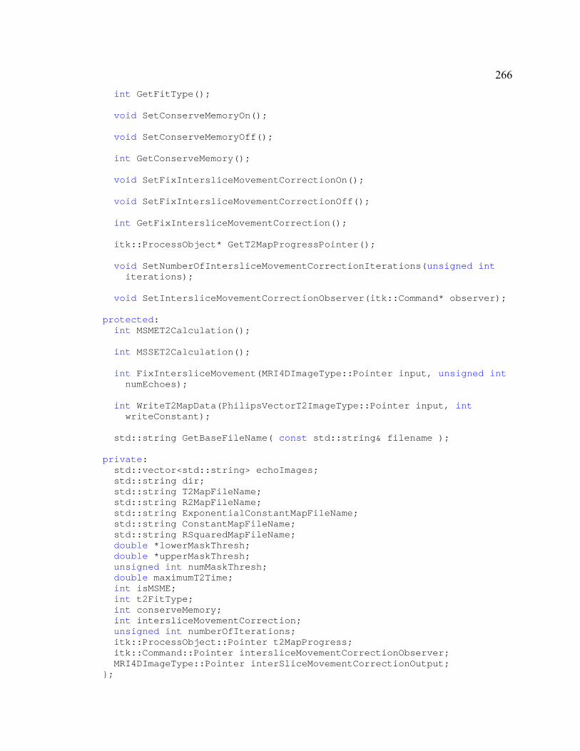
266 int GetFitType(); void SetConserveMemoryOn(); void SetConserveMemoryOff(); int GetConserveMemory(); void void SetFixIntersliceMovementCorrectionOff(); int GetFixIntersliceMovementCorrection(); itk::ProcessObject* GetT2MapProgressPointer(); void SetNumberOfIntersliceMovementCorrectionIterations(unsigned int iterations); void SetIntersliceMovementCorrectionObserver(itk::Command* observer); protected: int

int int FixIntersliceMovement(MRI4DImageType::Pointer input, unsigned int numEchoes); int WriteT2MapData(PhilipsVectorT2ImageType::Pointer input, int writeConstant); std::string GetBaseFileName( const std::string& filename ); private: std::vector<std::string> echoImages; std::string dir; std::string T2MapFileName; std::string R2MapFileName; std::string ExponentialConstantMapFileName; std::string ConstantMapFileName; std::string RSquaredMapFileName; double *lowerMaskThresh; double *upperMaskThresh; unsigned int numMaskThresh; double maximumT2Time; int isMSME; int t2FitType; int conserveMemory; int intersliceMovementCorrection; unsigned int numberOfIterations; itk::ProcessObject::Pointer t2MapProgress; itk::Command::Pointer intersliceMovementCorrectionObserver; MRI4DImageType::Pointer interSliceMovementCorrectionOutput; };

SetFixIntersliceMovementCorrectionOn();

MSMET2Calculation();

MSSET2Calculation();

267 #endif /* _PHILIPST2MAP_H */

B.2 PhilipsT2Map.cpp

/*************************************************************************** * $Id: PhilipsT2Map.cpp,v 1.36 2008/09/16 14:32:44 cnmrr Exp $ * * Wed Dec 21 13:17:43 2005 * Copyright 2005 The Pennsylvania State University * Email: [email protected] ****************************************************************************/ /* * This program is free software; you can redistribute it and/or modify * it under the terms of the GNU General Public License as published by * the Free Software Foundation; either version 2 of the License, or * (at your option) any later version. * * This program is distributed in the hope that it will be useful, * but WITHOUT ANY WARRANTY; without even the implied warranty of * MERCHANTABILITY or FITNESS FOR A PARTICULAR PURPOSE. See the * GNU Library General Public License for more details. * * You should have received a copy of the GNU General Public License * along with this program; if not, write to the Free Software * Foundation, Inc., 51 Franklin Street, Fifth Floor Boston, MA 02110-1301, USA */ #include "PhilipsT2Map.h" #include "itkPhilipsRECImageIO.h" #include "itkMRT2ParameterMap3DImageFilter.h" #include "itkExtractImageFilter.h" #include "itkImageToVectorImageFilter.h" #include "itkVectorIndexSelectionCastImageFilter.h" #include "itkThresholdImageFilter.h" #include "itkShiftScaleImageFilter.h" #include "itkShiftScaleInPlaceImageFilter.h" #include "itkResampleImageFilter.h" #include "itkAffineTransform.h" #include "itkLinearInterpolateImageFunction.h" #include "ImageRegistrationApp.h" #inclu

#inclu#include "itkSpatialOrientationAdapter.h" #include "itkOrientImageFilter.h" #include "itkMetaDataObject.h"

de "itkImageSliceConstIteratorWithIndex.h" #include "itkImageSliceIteratorWithIndex.h"

de "itkImageLinearIteratorWithIndex.h"

268 #include "itkProgressAccumulator.h" #include "itkReciprocalImageFilter.h" #include "vnl/vnl_vector_fixed.h" #include <algorithm> namespace itk { class ITK_EXPORT PhilipsT2MapProcessObject : public ProcessObject { public: type typedef ProcessObject Superclass; typedef SmartPointer<Self> Pointer; typedef SmartPointer<const Self> ConstPointer; itkTypeMacro(PhilipsT2MapProcessObject,ProcessObject); /** Standard New method. */ itkNewMacro(Self); protected: PhilipsT2MapProcessObject(){} virtual ~PhilipsT2MapProcessObject() {} private: PhilipsT2MapProcessObject(const Self&); //purposely not implemented void operator=(const Self&); //purposely not implemented }; } // end namespace itk // 4D types for multi-echo volumes. #define PHILIPS_REC_PIXEL_TYPE short typedef itk::PhilipsRECImageIO PhilipsRECImageIOType; typedef itk::Image<PHILIPS_REC_PIXEL_TYPE, 4> PhilipsREC4DImageType; typedef itk::ImageFileReader< PhilipsREC4DImageType > PhilipsREC4DImageFileReaderType; typedef itk::ThresholdImageFilter< MRI4DImageType > ThresholdMRI4DImageFilterType; typedef itk::ShiftScaleImageFilter<PhilipsREC4DImageType, MRI4DImageType> ShiftScaleMRI4DImageFilterType; typedef itk::ShiftScaleInPlaceImageFilter<MRI4DImageType> ShiftScaleInPlaceMRI4DImageFilterType; typedef itk::ExtractImageFilter<MRI4DImageType, MRIImageType > ExtractMRIImageFilterType; typedef itk::VectorContainer< unsigned int, ExtractMRIImageFilterType::Pointer > ExtractMRIImageFilterContainer // 3D types for single echo volumes. typedef itk::Image<PHILIPS_REC_PIXEL_TYPE, 3> PhilipsRECImageType; typedef itk::ImageFileReader< PhilipsRECImageType >

def PhilipsT2MapProcessObject Self;

Type;

269 PhilipsRECImageFileReaderType; typedef itk::VectorContainer< unsigned int, PhilipsRECImageFileReaderType::Pointer > PhilipsRECImageFileReaderContainerType; typedef itk::ThresholdImageFilter< MRIImageType >

iner< unsigned int, ThresholdMRIImageFilterType::Pointer > ThresholdMRIImageFilterContainerType; typedef itk::ShiftScaleImageFilter<PhilipsRECImageType, MRIImageType> ShiftScaleMRIImageFilterType; typedef itk::VectorContainer< unsigned int, ShiftScaleMRIImageFilterType::Pointer > ShiftScaleMRIImageFilterContainerType; typedef itk::ShiftScaleInPlaceImageFilter<MRIImageType> ShiftScaleInPlaceMRIImageFilterType; typedef itk::VectorContainer< unsigned int, ShiftScaleInPlaceMRIImageFilterType::Pointer > ShiftScaleInPlaceMRIImageFilterContainerType; typedef itk::ImageToVectorImageFilter<MRIImageType> MRIImageToVectorMRIImageFilterType; typedef itk::OrientImageFilter< MRIImageType, MRIImageType > OrientMRIImageFilterType; typedef itk::SpatialOrientationAdapter SpatialOrientationAdapterType; // Types used in both. typedef itk::MRT2ParameterMap3DImageFilter<DEFAULT_MRIMAGE_TYPE, DEFAULT_MRIMAGE_TYPE> MRT2ParameterMap3DImageFilterType; typedef itk::VectorIndexSelectionCastImageFilter< MRT2ParameterMap3DImageFilterType::OutputImageType, MRIImageType> VectorMRIImageToMRIImageFilterType; typedef itk::ReciprocalImageFilter<MRIImageType, MRIImageType> ReciprocalMRIImageFilterType; // Progress accumulator type. typedef itk::ProgressAccumulator ProgressAccumulatorType; // Insterslice movement correction types. typedef itk::ImageRegistrationApp<MRIImageType> MRIImageRegistrationAppType; typedef Affine3DTransformType; typedef itk::AffineTransform< double, 2 > Affine2DTransformType; typedef itk::LinearInterpolateImageFunction< MRI2DImageType, double > LinearInterpolatorMRI2DImageType; typedef itk::ImageSliceIteratorWithIndex< MRI4DImageType > MRI4DImageSliceIteratorWithIndexType; typedef itk::ImageLinearIteratorWithIndex< MRIImageType > MRIImageLinearIteratorType; typedef itk::ImageSliceConstIteratorWithIndex< MRIImageType > MRIImageSliceConstIteratorType; typedef itk::ExtractImageFilter< MRIImageType, MRI2DImageType >

ThresholdMRIImageFilterType; typedef itk::VectorConta

itk::AffineTransform< double, 3 >

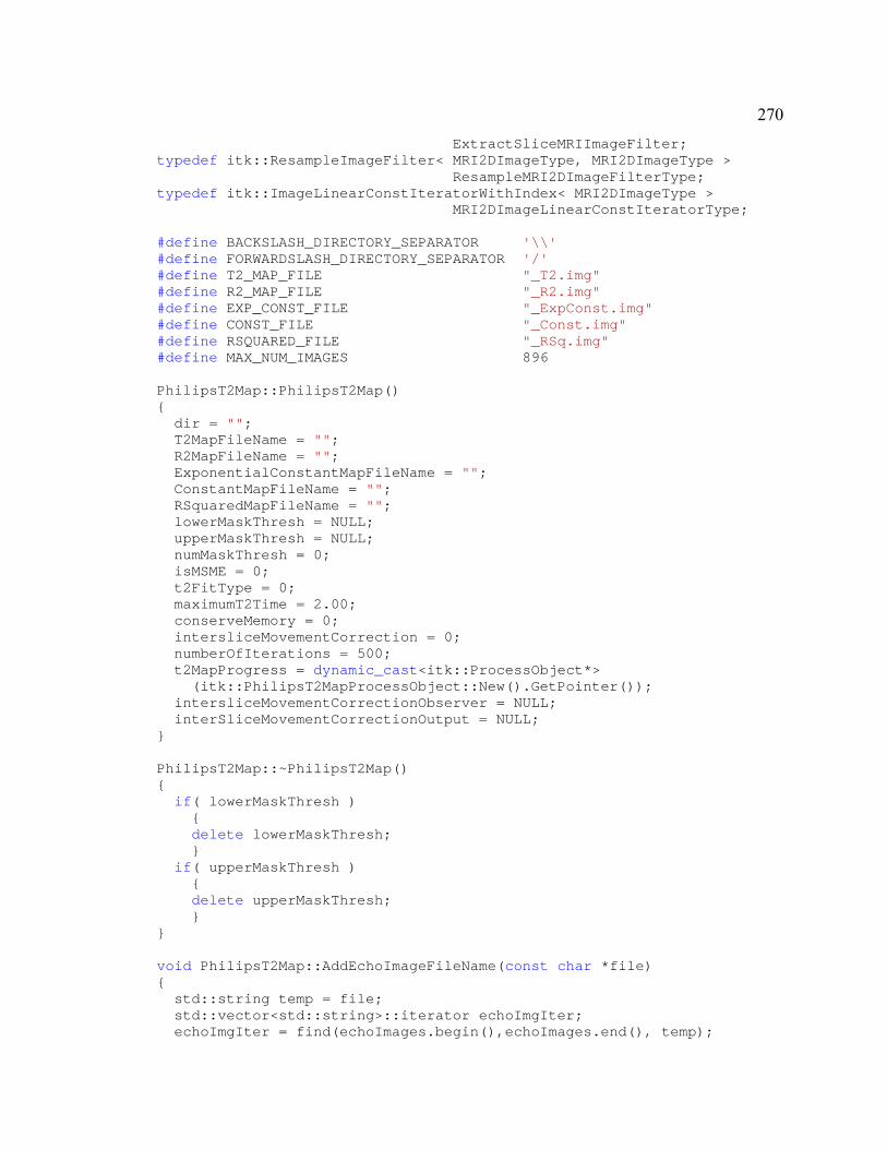
270 ExtractSliceMRIImageFilter; typedef itk::ResampleImageFilter< MRI2DImageType, MRI2DImageType >

MRI2DImageLinearConstIteratorType; #define BACKSLASH_DIRECTORY_SEPARATOR '\\' #define FORWARDSLASH_DIRECTORY_SEPARATOR '/' #define T2_MAP_FILE "_T2.img" #define R2_MAP_FILE "_R2.img" #define EXP_CONST_FILE "_ExpConst.img" #define CONST_FILE "_Const.img" #define RSQUARED_FILE "_RSq.img" #define MAX_NUM_IMAGES 896 PhilipsT2Map::PhilipsT2Map() { dir = ""; T2MapFileName = ""; R2MapFileName = ""; ExponentialConstantMapFileName = ""; ConstantMapFileName = ""; RSquaredMapFileName = ""; lowerMaskThresh = NULL; upperMaskThresh = NULL; numMaskThresh = 0; isMSME = 0; t2FitType = 0; maximumT2Time = 2.00; conserveMemory = 0; intersliceMovementCorrection = 0; numberOfIterations = 500; t2MapProgress = dynamic_cast<itk::ProcessObject*> (itk::PhilipsT2MapProcessObject::New().GetPointer()); intersliceMovementCorrectionObserver = NULL; interSliceMovementCorrectionOutput = NULL; } PhilipsT2Map::~PhilipsT2Map() { if( lowerMaskThresh ) { delete lowerMaskThresh; } if( upperMaskThresh ) { delete upperMaskThresh; } } void PhilipsT2Map::AddEchoImageFileName(const char *file) { std::string temp = file; std::vector<std::string>::iterator echoImgIter; echoImgIter = find(echoImages.begin(),echoImages.end(), temp);

ResampleMRI2DImageFilterType; typedef itk::ImageLinearConstIteratorWithIndex< MRI2DImageType >

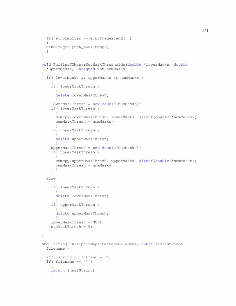
271 if( echoImgIter == echoImages.end() ) { echoImages.push_back(temp); } } void PhilipsT2Map::SetMaskThresholds(double *lowerMasks, double *upperMasks, unsigned int numMasks) { if( lowerMasks && upperMasks && numMasks ) { if( lowerMaskThresh ) { delete lowerMaskThresh; } lowerMaskThresh = new double[numMasks]; if( lowerMaskThresh ) { memcpy(lowerMaskThresh, lowerMasks, sizeof(double)*numMasks); numMaskThresh = numMasks; } if( upperMaskThresh ) { delete upperMaskThresh; } upperMaskThresh = new double[numMasks]; if( upperMaskThresh ) { memcpy(upperMaskThresh, upperMasks, sizeof(double)*numMasks); numMaskThresh = numMasks; } } else { if( lowerMaskThresh ) { delete lowerMaskThresh; } if( upperMaskThresh ) { delete upperMaskThresh; } lowerMaskThresh = NULL; numMaskThresh = 0; } } std::string PhilipsT2Map::GetBaseFileName( const std::string& filename ) { std::string nullString = ""; if( filename == "" ) { return (nullString); }

272 // Iterate through string replacing back-slashes with forward //slashes. std::string replaceBackslashes = filename; for(std::string::iterator iter=replaceBackslashes.begin(); iter!=replaceBackslashes.end(); iter++) { if(*iter == BACKSLASH_DIRECTORY_SEPARATOR) { *iter = FORWARDSLASH_DIRECTORY_SEPARATOR; } } // Find the last directory separator const std::string::size_type index = replaceBackslashes.find_last_of( FORWARDSLASH_DIRECTORY_SEPARATOR ); // This assumes that the final '.' in a file name is the delimiter // for the file's extension type const std::string::size_type it = replaceBackslashes.find_last_of( "." ); // This determines the file's type by creating a new string // who's value is the extension of the input filename // eg. "myimage.gif" has an extension of ".gif" std::string fileExt( replaceBackslashes, it, replaceBackslashes.length() ); std::string parentDirectory = replaceBackslashes.substr(0, index+1); std::string baseName = replaceBackslashes.substr(index+1, replaceBackslashes.length()-parentDirectory.length()- fileExt.length()); return ( baseName ); } void PhilipsT2Map::SetOutputDir(const char *d) { dir = d; } void PhilipsT2Map::SetMaximumT2Time(double time) { maximumT2Time = time; } std::string PhilipsT2Map::GetT2MapFileName() { T2MapFileName = dir; if( echoImages.size() ) { T2MapFileName += GetBaseFileName(echoImages[0]); } T2MapFileName += T2_MAP_FILE; return T2MapFileName; }

273 std::string PhilipsT2Map::GetR2MapFileName() { R2MapFileName = dir; if( echoImages.size() ) { R2MapFileName += GetBaseFileName(echoImages[0]); } R2MapFileName += R2_MAP_FILE; return R2MapFileName; } std::string PhilipsT2Map::GetExponentialConstantMapFileName() { ExponentialConstantMapFileName = dir; if( echoImages.size() ) { ExponentialConstantMapFileName += GetBaseFileName(echoImages[0]); } ExponentialConstantMapFileName += EXP_CONST_FILE; return ExponentialConstantMapFileName; } std::string PhilipsT2Map::GetConstantMapFileName() { ConstantMapFileName = dir; if( echoImages.size() ) { ConstantMapFileName += GetBaseFileName(echoImages[0]); } ConstantMapFileName += CONST_FILE; return ConstantMapFileName; } std::string PhilipsT2Map::GetRSquaredMapFileName() { RSquaredMapFileName = dir; if( echoImages.size() ) { RSquaredMapFileName += GetBaseFileName(echoImages[0]); } RSquaredMapFileName += RSQUARED_FILE; return RSquaredMapFileName; } int PhilipsT2Map::ExecuteT2MapCalculation() { // Check to see if all of the required info // is available. if( (dir == "") || (echoImages.empty()) ) { std::cerr << "ExecuteT2MapCalculation: The output directory must be set using SetOutputDir()" " and at least 1 image must be added via AddEchoImageFileName()" << std::endl; return 0;

274 } if( isMSME ) { return MSMET2Calculation(); } else { return MSSET2Calculation(); } } int PhilipsT2Map::MSMET2Calculation() { // Allocate readers & reorder filters. int numImages = echoImages.size(); int writeConst = 0; if( numImages != 1 ) { std::cerr << "MSMET2Calculation: Need to add exactly 1 MSME image via AddEchoImageFileName()" << std::endl; return 0; } if( (int)numMaskThresh > 1 ) { std::cerr << "MSMET2Calculation: Should only have 1 threshold value for an MSME image" << std::endl; return 0; } // Reset the progress. t2MapProgress->SetProgress(0); float numberOfStages = 1.0f; if( numMaskThresh ) { numberOfStages = 4.0f; } else { numberOfStages = 3.0f; } int num = 0; int extents[4] = {0}; // Create PAR/REC reader and check the file if it can be read. PhilipsRECImageIOType::Pointer imageIO = PhilipsRECImageIOType::New(); if( !imageIO->CanReadFile(echoImages[0].c_str()) ) { std::cerr << "MSMET2Calculation: Could not read PAR/REC file" << std::endl; return 0; } // Read the image information. imageIO->SetFileName(echoImages[0].c_str()); try {

275 imageIO->ReadImageInformation(); } catch( itk::ExceptionObject &err ) { std::cerr << "MSMET2Calculation: ExceptionObject caught !" << std::endl; std::cerr << err << std::endl; return 0; } // Make sure that the number of images // stored in the REC file matches the number of echoes. if( !itk::ExposeMetaData<int>(imageIO->GetMetaDataDictionary(), itk::PAR_MaxNumberOfEchoes,num) ) { std::cerr << "MSMET2Calculation: Could not determine the number of echoes" << std::endl; return 0; } // Get the image dimensions extents[0] = imageIO->GetDimensions(0); extents[1] = imageIO->GetDimensions(1); extents[2] = imageIO->GetDimensions(2); extents[3] = imageIO->GetDimensions(3); if( num > extents[3] ) { std::cerr << "MSMET2Calculation: The number of echoes is larger than the number of image blocks" << std::endl; return 0; } // Check to see if we have at least the magnitude image. int haveMagnitude = 0; int numberOfImageTypes = 0; PhilipsRECImageIOType::ImageTypesType imageTypes; if( !itk::ExposeMetaData<int>(imageIO->GetMetaDataDictionary(), itk::PAR_NumberOfImageTypes,numberOfImageTypes) ) { std::cerr << "MSMET2Calculation: Could not determine the number of image types" << std::endl; return 0; } if( !itk::ExposeMetaData<PhilipsRECImageIOType::ImageTypesType>( imageIO->GetMetaDataDictionary(),itk::PAR_ImageTypes,imageTypes) ) { std::cerr << "MSMET2Calculation: Could not get the image types vector" << std::endl; return 0; } for(int j=0; j<numberOfImageTypes; j++) { if( imageTypes[j] == 0 ) { haveMagnitude = 1; } } if( !haveMagnitude )

276 { std::cerr << "MSMET2Calculation: No magnitude image type detected in PAR file" << std::endl; return 0; } // Check to make sure we have just one scanning sequence, otherwise I have no idea how to process the // T2 map. int numberOfScanningSequences = 0; if( !itk::ExposeMetaData<int>(imageIO->GetMetaDataDictionary(), itk::PAR_NumberOfScanningSequences,numberOfScanningSequences) ) { std::cerr << "MSMET2Calculation: Could not determine the number of scanning sequences" << std::endl; return 0; } if( numberOfScanningSequences > 1 ) { std::cerr << "MSMET2Calculation: Cannot process a T2 map when the number of scanning sequences is greater than 1" << std::endl; return 0; } // Get rescale values. PhilipsRECImageIOType::ScanningSequenceImageTypeRescaleValuesContainerType::Pointer scanSequenceImageTypeRescaleValues = NULL; if( !itk::ExposeMetaData<PhilipsRECImageIOType::ScanningSequenceImageTypeRescaleValuesContainerType::Pointer> (imageIO->GetMetaDataDictionary(),itk::PAR_ScanningSequenceImageTypeRescaleValues,scanSequenceImageTypeRescaleValues) ) { std::cerr << "MSMET2Calculation: Could not get the rescale values for each scanning sequence and image types" << std::endl; return 0; } if( !scanSequenceImageTypeRescaleValues ) { std::cerr << "MSMET2Calculation: Received NULL scanning sequence/image types vector pointer from meta dictionary" << std::endl; return 0; } PhilipsRECImageIOType::ImageTypeRescaleValuesContainerType::Pointer rescaleValueVector = scanSequenceImageTypeRescaleValues->ElementAt(0); // Only 1 scanning sequence. if( !rescaleValueVector ) { std::cerr << "MSMET2Calculation: Received NULL rescale values vector pointer from meta dictionary" << std::endl; return 0; }

277 // Setup pipeline. PhilipsREC4DImageFileReaderType::Pointer philipsRECReader = PhilipsREC4DImageFileReaderType::New(); philipsRECReader->SetFileName(echoImages[0].c_str()); philipsRECReader->SetImageIO(imageIO); if( conserveMemory ) { philipsRECReader->ReleaseDataFlagOn(); } // Setup pipeline accumulator. ProgressAccumulatorType::Pointer progress = ProgressAccumulatorType::New(); progress->SetMiniPipelineFilter(t2MapProgress); // Change image to floating point value. ShiftScaleMRI4DImageFilterType::Pointer scaleOnly = NULL; ShiftScaleInPlaceMRI4DImageFilterType::Pointer shiftAndScale = NULL; PhilipsRECImageIOType::ImageTypeRescaleValuesType rescaleValues = rescaleValueVector->ElementAt(0); // Magnitude image will be the first element. if( (rescaleValues[2] != 0) && // scale slope (SS) (rescaleValues[1] != 0) ) // rescale slope (RS) { scaleOnly = ShiftScaleMRI4DImageFilterType::New(); scaleOnly->SetInput(philipsRECReader->GetOutput()); scaleOnly->SetScale(rescaleValues[1]); // RS if( conserveMemory ) { scaleOnly->ReleaseDataFlagOn(); } progress->RegisterInternalFilter(scaleOnly,1.0f/numberOfStages); shiftAndScale = ShiftScaleInPlaceMRI4DImageFilterType::New(); shiftAndScale->SetInput(scaleOnly->GetOutput()); shiftAndScale->SetShift(rescaleValues[0]); // rescale intercept (RI) shiftAndScale->SetScale(1.0/(rescaleValues[2]*rescaleValues[1])); // 1/(SS*RS) progress->RegisterInternalFilter( shiftAndScale,1.0f/numberOfStages); if( conserveMemory ) { shiftAndScale->ReleaseDataFlagOn(); } } else { std::cerr << "MSMET2Calculation: Invalid rescale values" << std::endl; return 0; } // Mask the images if the mask is set. ThresholdMRI4DImageFilterType::Pointer t2Mask = NULL; if( numMaskThresh )

278 { t2Mask = ThresholdMRI4DImageFilterType::New(); t2Mask->SetOutsideValue(0); t2Mask->SetInput(shiftAndScale->GetOutput()); if( conserveMemory ) { t2Mask->ReleaseDataFlagOn(); } // Shift and scale the thresholds also. t2Mask->ThresholdOutside((lowerMaskThresh[0]*rescaleValues[1] +rescaleValues[0])/(rescaleValues[2]*rescaleValues[1]), (upperMaskThresh[0]*rescaleValues[1] +rescaleValues[0])/(rescaleValues[2]*rescaleValues[1])); progress->RegisterInternalFilter(t2Mask,1.0f/numberOfStages); } // Fix inter-slice movement artifact if specified. if( intersliceMovementCorrection ) { try { if( numMaskThresh ) { t2Mask->Update(); } else { shiftAndScale->Update(); } } catch( itk::ExceptionObject &err ) { std::cerr << "MSMET2Calculation: ExceptionObject caught !" << std::endl; std::cerr << err << std::endl; return 0; } if( !FixIntersliceMovement((numMaskThresh)? t2Mask->GetOutput():shiftAndScale->GetOutput(),num) ) { std::cerr << "MSMET2Calculation: Inter-slice movement correction failed" << std::endl; return 0; } } MRT2ParameterMap3DImageFilterType::Pointer t2Map = MRT2ParameterMap3DImageFilterType::New(); switch(t2FitType) { case MRT2ParameterMap3DImageFilterType::LINEAR: t2Map->SetAlgorithm(MRT2ParameterMap3DImageFilterType::LINEAR); break; case MRT2ParameterMap3DImageFilterType::NON_LINEAR: t2Map->SetAlgorithm(

279 MRT2ParameterMap3DImageFilterType::NON_LINEAR); break; case MRT2ParameterMap3DImageFilterType::NON_LINEAR_WITH_CONSTANT: t2Map->SetAlgorithm( MRT2ParameterMap3DImageFilterType::NON_LINEAR_WITH_CONSTANT); writeConst = 1; break; } t2Map->SetMaxT2Time(maximumT2Time); progress->RegisterInternalFilter(t2Map,1.0f/numberOfStages); // Extract the volumes and echoes and set to T2 map filter. // DON'T EXTRACT THE FIRST ECHO! ExtractMRIImageFilterContainerType::Pointer extractVOI = ExtractMRIImageFilterContainerType::New(); extractVOI->resize(num-1); ExtractMRIImageFilterType::InputImageRegionType extractionRegion; ExtractMRIImageFilterType::InputImageSizeType extractionSize; extractionSize[0] = extents[0]; extractionSize[1] = extents[1]; extractionSize[2] = extents[2]; extractionSize[3] = 0; ExtractMRIImageFilterType::InputImageIndexType extractionIndex; extractionIndex[0] = 0; extractionIndex[1] = 0; extractionIndex[2] = 0; extractionRegion.SetSize(extractionSize); PhilipsRECImageIOType::EchoTimesContainerType::Pointer ptrToEchoes = NULL; if( !itk::ExposeMetaData<PhilipsRECImageIOType::EchoTimesContainerType::Pointer>(imageIO->GetMetaDataDictionary(), itk::PAR_EchoTimes,ptrToEchoes) ) { std::cerr << "MSMET2Calculation: Could not get the echo times" << std::endl; return 0; } if( !ptrToEchoes ) { std::cerr << "MSMET2Calculation: Received NULL echo times pointer from meta dictionary" << std::endl; return 0; } if( ptrToEchoes->size() != (unsigned int)num ) { std::cerr << "MSMET2Calculation: The size of the echo times vector does not match the number of echoes listed in the PAR file" << std::endl; return 0; } for(unsigned int i=1; i<(unsigned int)num; i++) { extractVOI->SetElement(i-1, ExtractMRIImageFilterType::New()); if( intersliceMovementCorrection )

280 { extractVOI->ElementAt(i-1)->SetInput(interSliceMovementCorrectionOutput); } else { if( numMaskThresh ) { extractVOI->ElementAt(i-1)->SetInput(t2Mask->GetOutput()); } else { extractVOI->ElementAt(i-1)->SetInput(shiftAndScale->GetOutput()); } } extractionIndex[3] = i; extractionRegion.SetIndex(extractionIndex); extractVOI->ElementAt(i-1)->SetExtractionRegion(extractionRegion); t2Map->AddMREchoImage(ptrToEchoes->ElementAt(i)/1000.0f, // convert to seconds extractVOI->ElementAt(i-1)->GetOutput()); } //Write output. if( !WriteT2MapData(t2Map->GetOutput(), writeConst) ) { std::cerr << "MSMET2Calculation: Could not write the results to file" << std::endl; return 0; } return 1; } int PhilipsT2Map::FixIntersliceMovement(MRI4DImageType::Pointer input, unsigned int numEchoes) { // Determine output region. MRI4DImageType::RegionType inputRegion = input->GetLargestPossibleRegion(); MRI4DImageType::SizeType inputSize = inputRegion.GetSize(); inputSize[3] = numEchoes; // Only work with the echo images. inputRegion.SetSize(inputSize); // Allocate output. interSliceMovementCorrectionOutput = MRI4DImageType::New(); interSliceMovementCorrectionOutput->SetRegions(inputRegion); interSliceMovementCorrectionOutput->SetSpacing(input->GetSpacing()); interSliceMovementCorrectionOutput->Allocate(); // Create output iterator. MRI4DImageSliceIteratorWithIndexType outputIterator(interSliceMovementCorrectionOutput, inputRegion); outputIterator.SetFirstDirection( 0 ); outputIterator.SetSecondDirection( 1 );

281 outputIterator.GoToBegin(); // Extract the volumes one by one. // Find the transformation for the first // volume then apply it to the subsequent volumes. Affine2DTransformType::InputPointType slice2DCenter; Affine2DTransformType::Pointer finalTransform = Affine2DTransformType::New(); Affine2DTransformType::ParametersType final2DParameters( finalTransform->GetNumberOfParameters()); ExtractMRIImageFilterType::Pointer extractVOI = ExtractMRIImageFilterType::New(); extractVOI->SetInput(input); ExtractMRIImageFilterType::InputImageRegionType extractionRegion; ExtractMRIImageFilterType::InputImageSizeType extractionSize; extractionSize[0] = inputSize[0]; extractionSize[1] = inputSize[1]; extractionSize[2] = inputSize[2]; extractionSize[3] = 0; ExtractMRIImageFilterType::InputImageIndexType extractionIndex; extractionIndex[0] = 0; extractionIndex[1] = 0; extractionIndex[2] = 0; extractionRegion.SetSize(extractionSize); // Reorient the image first. OrientMRIImageFilterType::Pointer orientImageFilter = OrientMRIImageFilterType::New(); orientImageFilter->SetInput(extractVOI->GetOutput()); orientImageFilter->UseImageDirectionOn(); MRI4DImageType::DirectionType inputDirection = input->GetDirection(); SpatialOrientationAdapterType::DirectionType dir; dir[0][0] = inputDirection[0][0]; dir[1][0] = inputDirection[1][0]; dir[2][0] = inputDirection[2][0]; dir[0][1] = inputDirection[0][1]; dir[1][1] = inputDirection[1][1]; dir[2][1] = inputDirection[2][1]; dir[0][2] = inputDirection[0][2]; dir[1][2] = inputDirection[1][2]; dir[2][2] = inputDirection[2][2]; SpatialOrientationAdapterType spatialOrientation; SpatialOrientationAdapterType::OrientationType coord_orient = spatialOrientation.FromDirectionCosines(dir); switch( coord_orient ) { case itk::SpatialOrientation::ITK_COORDINATE_ORIENTATION_RAI: // Fix axial orientation. orientImageFilter->SetDesiredCoordinateOrientation( itk::SpatialOrientation::ITK_COORDINATE_ORIENTATION_RPI); break; case itk::SpatialOrientation::ITK_COORDINATE_ORIENTATION_ASL: // Fix sagittal orientation. orientImageFilter->SetDesiredCoordinateOrientation( itk::SpatialOrientation::ITK_COORDINATE_ORIENTATION_PIR); break;

282 case itk::SpatialOrientation::ITK_COORDINATE_ORIENTATION_RSA: // Fix coronal orientation. orientImageFilter->SetDesiredCoordinateOrientation( itk::SpatialOrientation::ITK_COORDINATE_ORIENTATION_RIP); break; default: std::cout << "FixIntersliceMovement: Unhandled case: " << std::hex << (unsigned int)coord_orient << ". Need to fix this!" << std::endl; return 0; } for(unsigned int i=0; i<numEchoes; i++) { // Next volume. extractionIndex[3] = i; extractionRegion.SetIndex(extractionIndex); extractVOI->SetExtractionRegion(extractionRegion); try { orientImageFilter->Update(); } catch( itk::ExceptionObject &err ) { std::cerr << "FixIntersliceMovement: ExceptionObject caught !" << std::endl; std::cerr << err << std::endl; return 0; } // First break-up the volume into even and odd volumes. MRIImageType::Pointer oddVolume = MRIImageType::New(); MRIImageType::Pointer evenVolume = MRIImageType::New(); // First setup odd and even volumes. MRIImageType::RegionType oddRegion; MRIImageType::RegionType evenRegion; MRIImageType::RegionType::SizeType oddSize; MRIImageType::RegionType::SizeType evenSize; MRIImageType::PointType oddOrigin; MRIImageType::PointType evenOrigin; MRIImageType::SpacingType oddAndEvenSpacing; MRIImageType::RegionType requestedRegion = orientImageFilter->GetOutput()->GetRequestedRegion(); MRIImageType::SpacingType spacing = orientImageFilter->GetOutput()->GetSpacing(); // Spacing for both odd and even volumes. The inplane spacing stays // the same, but the z spacing is doubled. oddAndEvenSpacing = spacing; oddAndEvenSpacing[2] *= 2.0; // Odd volume. oddSize = requestedRegion.GetSize(); oddSize[2] = oddSize[2]/2;

283 oddRegion.SetSize( oddSize ); oddRegion.SetIndex( requestedRegion.GetIndex() ); oddVolume->SetRegions( oddRegion ); oddVolume->Allocate(); oddVolume->SetSpacing(oddAndEvenSpacing); oddOrigin[0] = 0; oddOrigin[1] = 0; oddOrigin[2] = 0; oddVolume->SetOrigin(oddOrigin); oddVolume->SetDirection( orientImageFilter->GetOutput()->GetDirection()); // Even volume. evenSize = requestedRegion.GetSize(); evenSize[2] = evenSize[2]/2 + evenSize[2]%2; evenRegion.SetSize( evenSize ); evenRegion.SetIndex( requestedRegion.GetIndex() ); evenVolume->SetRegions( evenRegion ); evenVolume->Allocate(); evenVolume->SetSpacing(oddAndEvenSpacing); evenOrigin[0] = 0; evenOrigin[1] = 0; evenOrigin[2] = -spacing[2]; evenVolume->SetOrigin(evenOrigin); evenVolume->SetDirection( orientImageFilter->GetOutput()->GetDirection()); // Now iterate slice by slice through the input volume and // put every other slice into the even and odd volumes. MRIImageSliceConstIteratorType inputIt( orientImageFilter->GetOutput(), requestedRegion ); MRIImageLinearIteratorType oddIt( oddVolume, oddVolume->GetRequestedRegion() ); MRIImageLinearIteratorType evenIt( evenVolume, evenVolume->GetRequestedRegion() ); inputIt.SetFirstDirection( 0 ); inputIt.SetSecondDirection( 1 ); oddIt.SetDirection( 0 ); evenIt.SetDirection( 0 ); int oddCount = 0; inputIt.GoToBegin(); oddIt.GoToBegin(); evenIt.GoToBegin(); while( !inputIt.IsAtEnd() ) { while ( !inputIt.IsAtEndOfSlice() ) { while ( !inputIt.IsAtEndOfLine() ) { if( oddCount == 1 ) { oddIt.Set( inputIt.Get() ); ++oddIt; } else

284 { evenIt.Set( inputIt.Get() ); ++evenIt; } ++inputIt; } inputIt.NextLine(); if( oddCount == 1 ) { oddIt.NextLine(); } else { evenIt.NextLine(); } } inputIt.NextSlice(); if( oddCount == 0 ) { oddCount = 1; } else { oddCount = 0; } } // First volume? if( i == 0 ) { // Yes, calculate transform. // Pass new origin and direction to output. MRIImageType::DirectionType outputDirection = orientImageFilter->GetOutput()->GetDirection(); MRIImageType::PointType outputOrigin = orientImageFilter->GetOutput()->GetOrigin(); MRI4DImageType::PointType inputOrigin; inputDirection[0][0] = outputDirection[0][0]; inputDirection[1][0] = outputDirection[1][0]; inputDirection[2][0] = outputDirection[2][0]; inputDirection[0][1] = outputDirection[0][1]; inputDirection[1][1] = outputDirection[1][1]; inputDirection[2][1] = outputDirection[2][1]; inputDirection[0][2] = outputDirection[0][2]; inputDirection[1][2] = outputDirection[1][2]; inputDirection[2][2] = outputDirection[2][2]; inputOrigin.Fill(0); inputOrigin[0] = outputOrigin[0]; inputOrigin[1] = outputOrigin[1]; inputOrigin[2] = outputOrigin[2]; interSliceMovementCorrectionOutput->SetOrigin( inputOrigin ); interSliceMovementCorrectionOutput->SetDirection( inputDirection ); // Setup registration.

285 MRIImageRegistrationAppType::Pointer registration = MRIImageRegistrationAppType::New(); // Set even as fixed image and odd as moving image. registration->SetFixedImage( evenVolume ); registration->SetMovingImage( oddVolume ); registration->SetMovingImageRegion( oddVolume->GetLargestPossibleRegion() ); // Set interpolator. registration->SetInterpolator(0); // Always linear transformation! // Set the initial transform to the center of mass of the two images. try { registration->RegisterUsingMass(); } catch( itk::ExceptionObject & err ) { std::cerr << "FixIntersliceMovement: ExceptionObject caught !" << std::endl; std::cerr << err << std::endl; return 0; } // Set the observer to monitor progress. if( intersliceMovementCorrectionObserver ) { registration->SetObserver(intersliceMovementCorrectionObserver ); } // Set the number of iterations. registration->SetAffineNumberOfIterations(numberOfIterations); // Set optimizer. registration->SetOptimizerToOnePlusOnePlusGradient(); try { registration->RegisterUsingAffine(); } catch( itk::ExceptionObject & err ) { std::cerr << "FixIntersliceMovement: ExceptionObject caught !" << std::endl; std::cerr << err << std::endl; return 0; } const double finalRotationCenterX = registration->GetFinalTransform()->GetCenter()[0]; slice2DCenter[0] = finalRotationCenterX; const double finalRotationCenterY = registration->GetFinalTransform()->GetCenter()[1]; slice2DCenter[1] = finalRotationCenterY; const double finalRotationCenterZ =

286 registration->GetFinalTransform()->GetCenter()[2]; const double finalTranslationX = registration->GetFinalTransform()->GetOffset()[0]; const double finalTranslationY = registration->GetFinalTransform()->GetOffset()[1]; const double finalTranslationZ = registration->GetFinalTransform()->GetOffset()[2]; const double bestValue = registration->GetAffineMetricValue(); // Print out results std::cout << "Result = " << std::endl; std::cout << " Center X = " << finalRotationCenterX << std::endl; std::cout << " Center Y = " << finalRotationCenterY << std::endl; std::cout << " Center Z = " << finalRotationCenterZ << std::endl; std::cout << " Translation X = " << finalTranslationX << std::endl; std::cout << " Translation Y = " << finalTranslationY << std::endl; std::cout << " Translation Z = " << finalTranslationZ << std::endl; std::cout << " Metric value = " << bestValue << std::endl; // Compute the rotation angle and scaling from SVD of the matrix // VNL returns the eigenvalues ordered from largest to smallest. Affine3DTransformType::ParametersType finalParameters = registration->GetFinalTransform()->GetParameters(); vnl_matrix<double> p(3, 3); p[0][0] = (double) finalParameters[0]; p[0][1] = (double) finalParameters[1]; p[0][2] = (double) finalParameters[2]; p[1][0] = (double) finalParameters[3]; p[1][1] = (double) finalParameters[4]; p[1][2] = (double) finalParameters[5]; p[2][0] = (double) finalParameters[6]; p[2][1] = (double) finalParameters[7]; p[2][2] = (double) finalParameters[8]; vnl_svd<double> svd(p); vnl_matrix<double> r(3, 3); r = svd.U() * vnl_transpose(svd.V()); double angle = asin(r[1][0]); std::cout << " Scale 1 = " << svd.W(0) << std::endl; std::cout << " Scale 2 = " << svd.W(1) << std::endl; std::cout << " Scale 3 = " << svd.W(2) << std::endl; std::cout << " Z Axis Rotation Angle (degrees) = " << angle * 45.0 / atan(1.0) << std::endl;

287 std::cout << " r[0][0] = " << r[0][0] << ", r[0][1] = " << r[0][1] << ", r[0][2] = " << r[0][2] <<std::endl; std::cout << " r[1][0] = " << r[1][0] << ", r[1][1] = " << r[1][1] << ", r[1][2] = " << r[1][2] <<std::endl; std::cout << " r[2][0] = " << r[2][0] << ", r[2][1] = " << r[2][1] << ", r[2][2] = " << r[2][2] <<std::endl; // Setup parameters for final transformation. final2DParameters[0] = cos(angle); final2DParameters[1] = sin(angle); final2DParameters[2] = -sin(angle); final2DParameters[3] = cos(angle); final2DParameters[4] = finalTranslationX; final2DParameters[5] = finalTranslationY; finalTransform->SetCenter( slice2DCenter ); finalTransform->SetParameters( final2DParameters ); } // Apply transform to each volume. // Move each odd slice to new position and put the even and odd slices // together again. MRIImageSliceConstIteratorType evenVolIt( evenVolume, evenVolume->GetLargestPossibleRegion() ); evenVolIt.SetFirstDirection( 0 ); evenVolIt.SetSecondDirection( 1 ); ExtractSliceMRIImageFilter::Pointer extractOddSlice = ExtractSliceMRIImageFilter::New(); extractOddSlice->SetInput(oddVolume); ExtractSliceMRIImageFilter::InputImageSizeType oddExtractedSize; oddExtractedSize[0] = inputSize[0]; oddExtractedSize[1] = inputSize[1]; oddExtractedSize[2] = 0; ExtractSliceMRIImageFilter::InputImageRegionType oddExtractedRegion; ExtractSliceMRIImageFilter::InputImageIndexType oddExtractedIndex; oddExtractedIndex[0] = 0; oddExtractedIndex[1] = 0; oddExtractedIndex[2] = 0; oddExtractedRegion.SetSize(oddExtractedSize); oddExtractedRegion.SetIndex(oddExtractedIndex); extractOddSlice->SetExtractionRegion(oddExtractedRegion); extractOddSlice->Update(); // Setup the interpolator for the resampling. LinearInterpolatorMRI2DImageType::Pointer interpolator = LinearInterpolatorMRI2DImageType::New(); interpolator->SetInputImage( extractOddSlice->GetOutput() ); ResampleMRI2DImageFilterType::Pointer resample = ResampleMRI2DImageFilterType::New(); resample->SetInput( extractOddSlice->GetOutput() ); resample->SetInterpolator( interpolator ); resample->SetTransform( finalTransform ); evenVolIt.GoToBegin(); for(unsigned int slice=0; slice < inputSize[2]; slice++) {

288 // Extract odd slice and apply shearing // and rotation to it before putting in // output volume. if( slice%2 ) { // Resample image. oddExtractedRegion.SetIndex(oddExtractedIndex); extractOddSlice->SetExtractionRegion(oddExtractedRegion); extractOddSlice->Update(); resample->SetSize( extractOddSlice->GetOutput()->GetBufferedRegion().GetSize() ); resample->SetOutputOrigin( extractOddSlice->GetOutput()->GetOrigin() ); resample->SetOutputSpacing( extractOddSlice->GetOutput()->GetSpacing() ); resample->Update(); oddExtractedIndex[2] = oddExtractedIndex[2]+1; } // Setup iterator for resampled odd slice. MRI2DImageLinearConstIteratorType oddIt(resample->GetOutput(), extractOddSlice->GetOutput()->GetBufferedRegion()); oddIt.SetDirection( 0 ); oddIt.GoToBegin(); while ( !outputIterator.IsAtEndOfSlice() ) { while ( !outputIterator.IsAtEndOfLine() ) { if( slice%2 ) { outputIterator.Set( oddIt.Get() ); ++oddIt; } else { outputIterator.Set( evenVolIt.Get() ); ++evenVolIt; } ++outputIterator; } outputIterator.NextLine(); if( slice%2 ) { oddIt.NextLine(); } else { evenVolIt.NextLine(); } } outputIterator.NextSlice(); } } return 1; }

289 int PhilipsT2Map::WriteT2MapData(PhilipsVectorT2ImageType::Pointer input, int writeConstant) { MRIImage *mriImage = new MRIImage(); int retVal = 0; VectorMRIImageToMRIImageFilterType::Pointer extractComp = VectorMRIImageToMRIImageFilterType::New(); extractComp->SetInput(input); // T2 map. extractComp->SetIndex(0); std::string writeFile = GetT2MapFileName(); mriImage->image = extractComp->GetOutput(); retVal = mriImage->saveMRIImage(writeFile,MRIIMAGE_FLOAT); // R2 map. ReciprocalMRIImageFilterType::Pointer r2Filter = ReciprocalMRIImageFilterType::New(); r2Filter->SetInput(extractComp->GetOutput()); writeFile = GetR2MapFileName(); mriImage->image = r2Filter->GetOutput(); retVal = (retVal)?mriImage->saveMRIImage(writeFile,MRIIMAGE_FLOAT):0; // Exponent Constant map. extractComp->SetIndex(1); mriImage->image = extractComp->GetOutput(); writeFile = GetExponentialConstantMapFileName(); retVal = (retVal)?mriImage->saveMRIImage(writeFile,MRIIMAGE_FLOAT):0; // Constant map. if( writeConstant ) { extractComp->SetIndex(2); writeFile = GetConstantMapFileName(); retVal = (retVal)?mriImage->saveMRIImage( writeFile,MRIIMAGE_FLOAT):0; } // Rsquared map. extractComp->SetIndex(3); writeFile = GetRSquaredMapFileName(); retVal = (retVal)?mriImage->saveMRIImage(writeFile,MRIIMAGE_FLOAT):0; // Clean up memory. delete mriImage; return retVal; } int PhilipsT2Map::MSSET2Calculation() { // Allocate 2DSEQ readers & reorder filters. unsigned int numImages = echoImages.size(); int writeConst = 0; if( numImages < 2 ) { std::cerr << "MSSET2Calculation: Must have at least 2 echo images for calculation" << std::endl;

290 return 0; } if( (numMaskThresh != 0) && (numMaskThresh != numImages) ) { std::cerr << "MSSET2Calculation: The number of threshold masks must match the number of images" << std::endl; return 0; } // Reset the progress. t2MapProgress->SetProgress(0); float numberOfStages = 0; if( numMaskThresh ) { numberOfStages = (float)numImages*3.0f+1.0f; } else { numberOfStages = (float)numImages*2.0f+1.0f; } unsigned int index = 0; PhilipsRECImageFileReaderContainerType::Pointer philipsRECReader = PhilipsRECImageFileReaderContainerType::New(); philipsRECReader->resize(numImages); ShiftScaleMRIImageFilterContainerType::Pointer scaleOnly = ShiftScaleMRIImageFilterContainerType::New(); scaleOnly->resize(numImages); ShiftScaleInPlaceMRIImageFilterContainerType::Pointer shiftAndScale = ShiftScaleInPlaceMRIImageFilterContainerType::New(); ThresholdMRIImageFilterContainerType::Pointer t2Mask = NULL; if( numMaskThresh ) { t2Mask = ThresholdMRIImageFilterContainerType::New(); t2Mask->resize(numImages); } MRIImageToVectorMRIImageFilterType::Pointer accumulateEchoImages = MRIImageToVectorMRIImageFilterType::New(); accumulateEchoImages->ReleaseDataFlagOn(); // Setup pipeline accumulator. ProgressAccumulatorType::Pointer progress = ProgressAccumulatorType::New(); progress->SetMiniPipelineFilter(t2MapProgress); // Check to see if all of the file names are readable. std::vector<std::string>::iterator echoImgIter; MRT2ParameterMap3DImageFilterType::EchoTimeContainerType::Pointer echoVector = MRT2ParameterMap3DImageFilterType::EchoTimeContainerType::New(); for(echoImgIter=echoImages.begin(); echoImgIter!=echoImages.end();echoImgIter++) { PhilipsRECImageIOType::Pointer imageIO =

291 PhilipsRECImageIOType::New(); if( !imageIO->CanReadFile((*echoImgIter).c_str()) ) { std::cerr << "MSSET2Calculation: Unable to read image: "<< *echoImgIter << std::endl; return 0; } else { // Read the image information. imageIO->SetFileName((*echoImgIter).c_str()); try { imageIO->ReadImageInformation(); } catch( itk::ExceptionObject &err ) { std::cerr << "MSSET2Calculation: ExceptionObject caught !" << std::endl; std::cerr << err << std::endl; return 0; } // WARNING: Boldly assuming that all of the images have the same size, // orign, spacing, direction, etc! int num = 0; philipsRECReader->SetElement(index, PhilipsRECImageFileReaderType::New()); philipsRECReader->ElementAt(index)->SetFileName( (*echoImgIter).c_str()); philipsRECReader->ElementAt(index)->SetImageIO(imageIO); if( conserveMemory ) { philipsRECReader->ElementAt(index)->ReleaseDataFlagOn(); } // Extract echoes. if( !itk::ExposeMetaData<int>(imageIO->GetMetaDataDictionary(), itk::PAR_MaxNumberOfEchoes,num) ) { std::cerr << "MSSET2Calculation: Could not determine the number of echoes" << std::endl; return 0; } if( num == 1 ) { PhilipsRECImageIOType::EchoTimesContainerType::Pointer ptrToEchoes = NULL; if( !itk::ExposeMetaData<PhilipsRECImageIOType::EchoTimesContainerType::Pointer>(imageIO->GetMetaDataDictionary(), itk::PAR_EchoTimes,ptrToEchoes) )

::endl; return 0;

{ std::cerr << "MSSET2Calculation: Could not get the echo time" std<<

292 } if( !ptrToEchoes ) { std::cerr << "MSSET2Calculation: pointer from meta dictionary" < return 0; } convert to seconds. } else { but has " << num << std::endl; return 0; } // Check to see if we have the magnitude image. int haveMagnitude = 0; int numberOfImageTypes = 0; PhilipsRECImageIOType::ImageTypesType imageTypes; if( !itk::ExposeMetaData<int>(imageIO->GetMetaDataDictionary(), i of image types" << std::endl;

Received NULL echo time < std::endl;

echoVector->push_back(ptrToEchoes->ElementAt(0)/1000.0f); //

std::cerr << "MSSET2Calculation: Image should have only 1 echo,

tk::PAR_NumberOfImageTypes,numberOfImageTypes) ) { std::cerr << "MSSET2Calculation: Could not determine the number

return 0; } if( !itk::ExposeMetaData<PhilipsRECImageIOType::ImageTypesType>(imageIO->GetMetaDataDictionary(), itk::PAR_ImageTypes,imageTypes) ) { std::cerr << "MSSET2Calculation: Could not get the image types vector" << std::endl; return 0; } for(unsigned int j=0; j<(unsigned int)numberOfImageTypes; j++) { if( imageTypes[j] == 0 ) { haveMagnitude = 1; } } if( !haveMagnitude ) { std::cerr << "MSSET2Calculation: This PAR/REC image does not have the magnitude image" << std::endl; return 0; } // Check to make sure we have just one scanning sequence, otherwise I have no idea how to process the // T2 map. int numberOfScanningSequences = 0; if( !itk::ExposeMetaData<int>(imageIO->GetMetaDataDictionary(), itk::PAR_NumberOfScanningSequences,numberOfScanningSequences) )

293 { std::cerr << "MSSET2Calculation: Could not determine the number of scanning sequences" << std::endl; return 0; } if( numberOfScanningSequences > 1 ) {

T2 map when the number of scanning sequences is greater than 1" << std::endl; return 0; } // Shift and scale image, get rescale values first. PhilipsRECImageIOType::ScanningSequenceImageTypeRescaleValuesContainerType::Pointer scanSequenceImageTypeRescaleValues = NULL; if( !itk::ExposeMetaData<PhilipsRECImageIOType::ScanningSequenceImageTypeRescaleValuesContainerType::Pointer> (imageIO->GetMetaDataDictionary(),itk::PAR_ScanningSequenceImageTypeRescaleValues,scanSequenceImageTypeRescaleValues) ) { std::cerr << "MSSET2Calculation: Could not get the rescale values

image types" << std::endl; return 0; } if( !scanSequenceImageTypeRescaleValues ) { std::cerr << "MSSET2Calculation: Received NULL scanning

return 0; } PhilipsRECImageIOType::ImageTypeRescaleValuesContainerType::Pointer rescaleValueVector = scanSequenceImageTypeRescaleValues->ElementAt(0); // Only 1 scanning sequence. if( !rescaleValueVector ) { std::cerr << "MSSET2Calculation: Received NULL rescale values vector pointer from meta dictionary" << std::endl; return 0; } PhilipsRECImageIOType::ImageTypeRescaleValuesType rescaleValues

(rescaleValues[1] != 0) ) // rescale slope (RS) { scaleOnly->SetElement(index,ShiftScaleMRIImageFilterType::New()); scaleOnly->ElementAt(index)->SetInput( philipsRECReader->ElementAt(index)->GetOutput()); scaleOnly->ElementAt(index)->SetScale(rescaleValues[1]); // RS if( conserveMemory ) { scaleOnly->ElementAt(index)->ReleaseDataFlagOn(); } progress->RegisterInternalFilter(

std::cerr << "MSSET2Calculation: Cannot process a

for each scanning sequence and

sequence/image types vector pointer from meta dictionary" << std::endl;

= rescaleValueVector->ElementAt(0); if( (rescaleValues[2] != 0) && // scale slope (SS)

294 scaleOnly->ElementAt(index),1.0f/numberOfStages); shiftAndScale->SetElement(index,

scaleOnly->ElementAt(index)->GetOutput()); shiftAndScale->ElementAt(index)->SetShift(rescaleValues[0]); // re shiftAndScale->ElementAt(index)->SetScale( 1.0/(rescaleValues[2]*rescaleValues[1])); // 1/(SS*RS) if( conserveMemory ) { shiftAndScale->ElementAt(index)->ReleaseDataFlagOn(); } progress->RegisterInternalFilter(shiftAndScale->ElementAt(index), else { std::cerr << "MSSET2Calculation: Invalid resacle values" << std::endl; return 0; } // Threshold image. if( numMaskThresh ) { t2Mask->SetElement(index, ThresholdMRIImageFilterType::New()); t2Mask->ElementAt(index)->SetOutsideValue(0); t2Mask->ElementAt(index)->SetInput( shiftAndScale->ElementAt(index)->GetOutput()); // Shift and scale the thresholds also. t2Mask->ElementAt(index)->ThresholdOutside( (lowerMaskThresh[index]*rescaleValues[1]+rescaleValues[0]) /(rescaleValues[2]*rescaleValues[1]), (upperMaskThresh[index]*rescaleValues[1]+rescaleValues[0]) /(rescaleValues[2]*rescaleValues[1])); if( conserveMemory ) { t2Mask->ElementAt(index)->ReleaseDataFlagOn(); } progress->RegisterInternalFilter(t2Mask->ElementAt(index), 1.0f/numberOfStages); } // Put all of the echo images into a VectorImage. if( numMaskThresh ) { accumulateEchoImages->SetNthInput(index, t2Mask->ElementAt(index)->GetOutput()); } else { accumulateEchoImages->SetNthInput(index, shiftAndScale->ElementAt(index)->GetOutput()); } }

ShiftScaleInPlaceMRIImageFilterType::New()); shiftAndScale->ElementAt(index)->SetInput(

scale intercept (RI)

1.0f/numberOfStages); }

295 } // Need to update at this point or we will get an exception. try { accumulateEchoImages->Update(); } catch( itk::ExceptionObject &err ) { std::cerr << "MSSET2Calculation: ExceptionObject caught !" << std::endl; std::cerr << err << std::endl; return 0; } // Do T2 fitting now. MRT2ParameterMap3DImageFilterType::Pointer t2Map = MRT2ParameterMap3DImageFilterType::New(); t2Map->SetMREchoImage(echoVector, accumulateEchoImages->GetOutput()); progress->RegisterInternalFilter(t2Map,1.0f/numberOfStages); switch( t2FitType ) { t2Map->SetAlgorithm(MRT2ParameterMap3DImageFilterType::LINEAR); break; case MRT2ParameterMap3DImageFilterType::NON_LINEAR: t2Map->SetAlgorithm( MRT2ParameterMap3DImageFilterType::NON_LINEAR); break; case MRT2ParameterMap3DImageFilterType::NON_LINEAR_WITH_CONSTANT: t2Map->SetAlgorithm( MRT2ParameterMap3DImageFilterType::NON_LINEAR_WITH_CONSTANT); writeConst = 1; break; } t2Map->SetMaxT2Time(maximumT2Time); //Write output. if( !WriteT2MapData(t2Map->GetOutput(), writeConst) ) { std::cerr << "MSSET2Calculation: Could not write the results to file" << std::endl; return 0; } return 1; } void PhilipsT2Map::SetMSMEOn() { isMSME = 1; } void PhilipsT2Map::SetMSMEOff() {

index++;

case MRT2ParameterMap3DImageFilterType::LINEAR:

296 isMSME = 0; } int PhilipsT2Map::GetMSME() { } void PhilipsT2Map::SetFitType(int fit) { t2FitType = fit; } in{ return t2FitType; } void PhilipsT2Map::SetConserveMemoryOn() { conserveMemory = 1; } void PhilipsT2Map::SetConserveMemoryOff() { conserveMemory = 0; } int PhilipsT2Map::GetConserveMemory() { return conserveMemory; } void PhilipsT2Map::SetFixIntersliceMovementCorrectionOn() { intersliceMovementCorrection = 1; } void PhilipsT2Map::SetFixIntersliceMovementCorrectionOff() { intersliceMovementCorrection = 0; } int PhilipsT2Map::GetFixIntersliceMovementCorrection() { return intersliceMovementCorrection; } itk::ProcessObject* PhilipsT2Map::GetT2MapProgressPointer() { return dynamic_cast<itk::ProcessObject*>(t2MapProgress.GetPointer()); } void PhilipsT2Map::SetNumberOfIntersliceMovementCorrectionIterations( unsigned int iterations)

return isMSME;

t PhilipsT2Map::GetFitType()

297

{ } void PhilipsT2Map::SetIntersliceMovementCorrectionObserver(itk::Command* observer) { intersliceMovementCorrectionObserver = observer; }

numberOfIterations = iterations;

Appendix C

Process Philips DTI tcl and C++ Source Code

The following source code is used to process Philips DTI image data stored in the

PAR/REC image format. It supports PAR versions <= 4.1. For PAR versions that are

not equal to 4.1, where the gradient values are stored in the PAR file, it assumes gradient

values for the default DTI sequence. It runs in Linux and uses the FMRIB’s Diffusion

Toolkit (FDT) (http://www.fmrib.ox.ac.uk/fsl/fdt/index.html) for eddy current correction

and key tensor calculation steps. It also uses parts of the MR Parameter Map Suite

described in Appendix A.

C.1 call_sourcePhilipsDTIFit.sh

#!/bin/sh echo "FSLOUTPUTTYPE is ${FSLOUTPUTTYPE}" input_csv=$1 sessionID=`date +%m%d%Y.%H%M%S` echo "Input csv file: $input_csv" echo "Session ID: $sessionID" tclsh ${PHILIPSDTIFIT_DIR}/sourcePhilipsDTIFit.tcl $input_csv $sessionID PhilipsDTIFit:Go >& ${PHILIPSDTIFIT_DIR_LOG}/log_call_sourcePhilipsDTIFit

al cond global PAR_INFO puputs "argv: $argv"

C.2 sourcePhilipsDTIFit.tcl

global fl glob

ts "argc: $argc"

http://www.fmrib.ox.ac.uk/fsl/fdt/index.html

299 set fl(dir_PHILIPSDTIFIT) $env(PHILIPSDTIFIT_DIR) set fl(dir_log) $env(PHILIPSDTIFIT_DIR_LOG) set fl(dir_base) $env(PHILIPSDTIFIT_DATA_BASE_DIR) set FSLDIR $env(FSLDIR) set PAR_INFO(PAR_Filename) "" set PAR_INFO(B0_Index) 0 set fl(csv_file) [lindex $argv 0] set sessionID [lindex $argv 1].[exec uname -n] set p [lindex $argv 2] set fl(dir_log) $fl(dir_log)/$sessionID if { ![file isdirectory $fl(dir_log)] } { set status [catch {exec mkdir $fl(dir_log)} ErrorMessage] if {$status != 0} { puts "Cannot create directory: $fl(dir_log)\nError is: $ErrorMessage" puts "Exiting ..." exit } } set this PhilipsDTIFit cd $fl(dir_PHILIPSDTIFIT) source PhilipsDTIFit.tcl PhilipsDTIFit:init if { $argc == 3 } { set status [$p] } elseif { $argc == 4 } { set status [$p [lindex $argv 3]] } else { set status 0 } if { $status == $cond(normal) } { PhilipsDTIFit:log $this "Done." } elseif { $status == $cond(error) } { PhilipsDTIFit:log $this "Done, with errors." $cond(error) } exit

C.3 PhilipsDTIFit.tcl

# This tcl script will use FSL's FDT library as well as code developed # in the CNMRR to reconstruct Philips DTI data. # Author: Don Bigler

300 # Feb. 02, 2008 # Copyright Penn State University proc PhilipsDTIFit:Go { } { global cond global fl set this "PhilipsDTIFit:Go" PhilipsDTIFit:log $this "Entered." # Populate our data model so that we have detailed info # on what data/images we will process. set status [PhilipsDTIFit:Read lst_PhilipsData] if { $status != $cond(normal) } { return $cond(error) } PhilipsDTIFit:Iterator:FileList "PhilipsDTIFit:FileKL:Process" lst_PhilipsData return $cond(normal) } proc PhilipsDTIFit:CSV:Write { fnabs a } { upvar $a l_a set str_k "MIISCPatientID,MIISCPatientAge,MIISCPatientSex,MIISCStudyID,MIISCPatientGroup,MIISCImageType,MIISCSequenceName,MIISCImageAcquisitionDate" set str_v "$l_a(MIISCPatientID),$l_a(MIISCPatientAge),$l_a(MIISCPatientSex),$l_a(MIISCStudyID),$l_a(MIISCPatientGroup),$l_a(MIISCImageType),$l_a(MIISCSequenceName),$l_a(MIISCImageAcquisitionDate)" set fd [open $fnabs w] puts $fd $str_k puts $fd $str_v close $fd } # The purpose is to apply a proc (whose name is specified by # the p variable) to a collection of 'file' object instances, # but the implementation is such that this collection is entered # (see: the lst variable) by instead specifying a list of 'directory' # object instances (each of which holds a FileList key that holds # a list of 'file' object instances we want). This way, it becomes # possible to simply pass the full data tree of the program # to the proc, rather than having to first extract from it # a list of 'file' object instances to be passed to this proc; # however, this behavior of the proc may be changed later. proc PhilipsDTIFit:Iterator:FileList { p lst } { global cond global fl upvar $lst l_lst set this "PhilipsDTIFit:Iterator:FileList" set v_FileList [PhilipsDTIFit:kl:get l_lst FileList]

301 foreach kl_File $v_FileList { $p kl_File } } # Member function to 'process' a 'file' object. # Note: The 'file' object is being given the name "FileKL" in proc names. # # This proc is the main entry point into the processing # of an individual image file, or more specifically of a 'file' # object instance which is a Keyed List (i.e. the # kl_File variable). Make sure the "img" key of the Keyed List

hilipsDTIFit:FileKL:Process { kl_File } {

_File: $l_kl_File" le "par"] e "PARVersion"]

:kl:get l_kl_File

"]

geAcquisitionDate"]

set status [PhilipsDTIFit:DataFile:Process a] if { $status == $cond(error) } { return $cond(error) } return $cond(normal) } proc PhilipsDTIFit:DataFile:Process { a } { global cond global fl global PAR_INFO upvar $a l_a set this "PhilipsDTIFit:DataFile:Process"

# has already been set before calling this proc. proc P global fl global cond upvar $kl_File l_kl_File set this "PhilipsDTIFit:FileKL:Process" PhilipsDTIFit:log $this "l_kl set a(fnabs_in) [PhilipsDTIFit:kl:get l_kl_Fi set a(par_ver) [PhilipsDTIFit:kl:get l_kl_Fil set a(MIISCPatientID) [PhilipsDTIFit:kl:get l_kl_File "MIISCPatientID"] set a(MIISCPatientAge) [PhilipsDTIFit:kl:get l_kl_File "MIISCPatientAge"] set a(MIISCPatientSex) [PhilipsDTIFit"MIISCPatientSex"] set a(MIISCStudyID) [PhilipsDTIFit:kl:get l_kl_File "MIISCStudyID set a(MIISCPatientGroup) [PhilipsDTIFit:kl:get l_kl_File "MIISCPatientGroup"] set a(MIISCImageType) [PhilipsDTIFit:kl:get l_kl_File "MIISCImageType"] set a(MIISCSequenceName) [PhilipsDTIFit:kl:get l_kl_File "MIISCSequenceName"] set a(MIISCImageAcquisitionDate) [PhilipsDTIFit:kl:get l_kl_File "MIISCIma PhilipsDTIFit:log $this "file: $a(fnabs_in)" set a(fnabs_log) [PhilipsDTIFit:PAR:2log $a(fnabs_in)]

302 # Now ready to switch the logging to datafile-specific logging, so do it. set fl(logfile) $l_a(fnabs_log) set rootname [PhilipsDTIFit:Filename:PreExtension $l_a(fnabs_in)] # Create directory for processing if possible, otherwise # exit with an error. set fl(dir_out) [PhilipsDTIFit:Filename:directory $l_a(fnabs_in)]/fdt_[set rootname] if { ![file isdirectory $fl(dir_out)] } { PhilipsDTIFit:log $this "mkdir $fl(dir_out)" set status [catch { exec mkdir $fl(dir_out) >>& $fl(logfile) } ErrorMessage] if { $status != 0 } { return [PhilipsDTIFit:log $this $ErrorMessage $cond(error)] } } # Store PAR file name for future use set PAR_INFO(PAR_Filename) $l_a(fnabs_in) # Store B0 index for future use if { [ catch { exec sh -c "philipsparinfo $PAR_INFO(PAR_Filename) -b0" } index ] } { PhilipsDTIFit:log $this "Failed to get volume index of B0 using philipsparinfo" return $cond(error) } set PAR_INFO(B0_Index) [ lindex $index 0 ] PhilipsDTIFit:log $this "B0 volume index is $PAR_INFO(B0_Index)" # Write gradient and B-value files. PhilipsDTIFit:BVal:Write l_a PhilipsDTIFit:BVec:Write l_a set CPTA_fnabs_in $l_a(fnabs_in) set status [PhilipsDTIFit:ConvertPhilipsToAnalyze l_a] if { $status == $cond(error) } { return $cond(error) } set CPTA_fnabs_out $l_a(fnabs_out) set l_a(fnabs_in) $CPTA_fnabs_out set status [PhilipsDTIFit:RemoveLastVolume l_a] if { $status == $cond(error) } { return $cond(error) } set RLV_fnabs_out $l_a(fnabs_out) set l_a(fnabs_in) $RLV_fnabs_out set status [PhilipsDTIFit:ThresholdImage l_a] if { $status == $cond(error) } { return $cond(error) } set TI_fnabs_out $l_a(fnabs_out) set l_a(fnabs_in) $TI_fnabs_out set status [PhilipsDTIFit:EddyCurrentCorrection l_a] if { $status == $cond(error) } { return $cond(error) } set ECC_fnabs_out $l_a(fnabs_out)

303 set l_a(fnabs_in) $ECC_fnabs_out set status [PhilipsDTIFit:CreateB0 l_a] if { $status == $cond(error) } { return $cond(error) } set CB0_fnabs_out $l_a(fnabs_out) set l_a(fnabs_in) $CB0_fnabs_out set status [PhilipsDTIFit:CreateBrainMaskFromB0 l_a] if { $status == $cond(error) } { return $cond(error) } set CBMFB0_fnabs_out $l_a(fnabs_out) set l_a(fnabs_in) $CBMFB0_fnabs_out set status [PhilipsDTIFit:DoDTIFit l_a] if { $status == $cond(error) } { return $cond(error) } return $cond(normal) } proc PhilipsDTIFit:ConvertPhilipsToAnalyze { a } { global fl global cond global PAR_INFO upvar $a l_a set this "PhilipsDTIFit:ConvertPhilipsToAnalyze" PhilipsDTIFit:Filename:in2out "ana" l_a PhilipsDTIFit:log $this "convertphilipstoanalyze $l_a(fnabs_in) $l_a(fnabs_out)" set status [catch { exec convertphilipstoanalyze $l_a(fnabs_in) $l_a(fnabs_out) >>& $fl(logfile) } ErrorMessage] if { $status != 0 } { return [PhilipsDTIFit:log $this $ErrorMessage $cond(error)] } set rv [PhilipsDTIFit:OutputFileOK $l_a(fnabs_out) $this] return $rv } proc PhilipsDTIFit:RemoveLastVolume { a } { global FSLDIR global fl global cond upvar $a l_a set this "PhilipsDTIFit:RemoveLastV PhilipsDTIFit:Filename:in2out "noaverage" l_a PhilipsDTIFit:log $this "$FSLDIR/bin/avwsplit $l_a(fnabs_in) $fl(dir_out)/vol" set status [catch { exec $FSLDIR/bin/avwsplit $l_a(fnabs_in) $fl(dir_out)/vol >>& $fl(logfile) } ErrorMessage] if { $status != 0 return [PhilipsDTIFit:log $this $ErrorMessage $cond(error)] }

olume"

} {

304 # Remerge all but the last volume. set volumes [glob $fl(dir_out)/vol*.hdr] set volumes [lsor set last [expr { PhilipsDTIFit:log $this "Last volume index $last" set volumes [lrange $volumes 0 $las set param_list "" foreach vol $volu append param_list $vol " " } PhilipsDTIFit:log $this "${FSLDIR}/bin/avwmerge -t $l_a(fnabs_out) $param_list" set status [catch { eval exec ${FSLDIR}/bin/avwmerge -t $l_a(fnabs_out) $volumes >>& $fl(logfile) } ErrorMessage] if { $status != 0 return [PhilipsDTIFit:log $this $ErrorMessage $cond(error)] } # Remove the split volumes now that they are merged again. set volumes [glob foreach set status [PhilipsDTIFit:File:Remove $vol $this] if { $status == $cond(error) } { return $cond(error) } } # Remove the input because it is not needed and it uses up lots of disk space set volumes [glob [PhilipsDTIFit:Filename:WithoutExtension $l_a(fnabs_in)].*] foreach vol $volumes { set status [PhilipsDTIFit:File:Remove $vol $this] if { $status == $cond(error) } { return $cond(error) } } set rv [PhilipsDTIFit:OutputFileOK $l_a(fnabs_out) $this] return $rv } proc PhilipsDTIFit:EddyCurrentCorrection { a } { global FSLDIR global fl global cond global PAR_INFO upvar $a l_a set this "PhilipsDTIFit:EddyCurrentCorrection" PhilipsDTIFit:log $this "${FSLDIR}/bin/eddy_correct $l_a(fnabs_in) $fl(dir_out)/data $PAR_INFO(B0_Index)" set status [catch { exec ${FSLDIR}/bin/eddy_correct $l_a(fnabs_in) $fl(dir_out)/data $PAR_INFO(B0_Index) >>& $fl(logfile) } ErrorMessage] if { $status != 0 } { return [PhilipsDTIFit:log $this $ErrorMessage $cond(error)] }

t $volumes] [llength $volumes]-2 }]

t]

mes {

} {

$fl(dir_out)/vol*] vol $volumes {

.

305 # Remove the input because it is not needed and it uses up lots of disk space. set volumes [glob [PhilipsDTIFit:Filename:WithoutExtension $l_a(fnabs_in)].*] foreach vol $volu set status [PhilipsDTIFit:File:Remove $vol $this] if { $status == $cond(error) } { return $cond(error) } } set rv [PhilipsDTIFit:OutputFileOK $fl(dir_out)/data.img $this] return $rv } proc PhilipsDTIFit: global FSLDIR global fl global cond global PAR_INFO upvar $a l_a set this "Philips set par_ver [expr {$l_a(par_ver)}] PhilipsDTIFit:log $this "PAR Version: $par_ver" set reference $PA # Different Bvec depending on PAR v if { $par_ver < 4.1 } { set reference 0 } PhilipsDTIFit:log $this "${FSLDIR}/bin/avwsplit $fl(dir_out)/data $fl(dir_out)/vol" set status [catch { exec ${FSLDIR}/bin/avwsplit $fl(dir_out)/data $fl(dir_out)/vol >> if { $status != 0 return [PhilipsDTIFit:log $this $ErrorMessage $cond(error)] } set b0name $fl(dir_out)/$l_a(MIISCPatientID)$l_a(MIISCPatientAge)$l_a(MIISCPatientSex)_B0 set status [PhilipsDTIFit:File:Move $l_a(dir_in)/vol00$reference.hdr $b0name.hdr $this] if { $status == $cond(error) } { return $cond(error) } set status [PhilipsDTIFit:File:Move $l_a(dir_in)/vol00$reference.img $b0name.img $this] if { $status == $cond(error) } { return $cond(error) } # Remove the split volumes now that we have renamed the B0 image. set volumes [glob foreach vol $volum set status [Phil

mes {

CreateB0 { a } {

DTIFit:CreateB0"

R_INFO(B0_Index)

ersion

0

& $fl(logfile) } ErrorMessage] } {

$fl(dir_out)/vol*] es { ipsDTIFit:File:Remove $vol $this]

306 if { $status == $cond(error) } { return $cond(error) } } # Write csv file for b0 set temp_a(MIISCImageType) "dtib0" foreach value {MIIMIISCStudyID MIISCPatientGroup \ MIISCSequenceName MIISCImageAcquisitionDate} { set temp_a($valu } PhilipsDTIFit:CSV:Write $b0name.csv set rv [PhilipsDTIFit:OutputFileOK $b0name.img $this] return $rv } proc PhilipsDTIFit:CreateBrainMaskFromB0 { a } { global FSLDIR global fl global cond upvar $a l_a set this "PhilipsD set b0name $fl(dir_out)/$l_a(MIISCPatientID)$l_a(MIISCPatientAge)$l_a(MIISCPatientSex)_B0 PhilipsDTIFit:log $this "${FSLDIR}/bin/bet $b0name $fl(dir_out)/nodif_brain -m -f 0.3" set status [catch { exec ${FSLDIR}/bin/bet $b0name $fl(dir_out)/nodif_brain -m -f 0.3 >>& $fl(logfile) } ErrorMessage] if { $status != 0 } { return [PhilipsDTIFit:log $this $ErrorMessage $cond(error)] } # Mask the original b0 image. #PhilipsDTIFit:log $this "$FSLDIR/bin/avwmaths++ $b0name -mas $fl(dir_out)/nodif_brain_mask.img $b0name" #set status [catch { exec $FSLDIR/bin/avwmaths++ $b0name -mas $fl(dir_out)/nodif_brain_mask.img $b0name >>& $fl(logfile) } ErrorMessage] #if { $status != 0 } { #return [PhilipsDTIFit:log $this $ErrorMessage $cond(error)] #} set rv [PhilipsDTIFit:OutputFileOK $fl(dir_out)/nodif_brain_mask.img $this] return $rv } proc PhilipsDTIFit:ThresholdImage { a } { global FSLDIR global fl global cond upvar $a l_a

SCPatientID MIISCPatientAge MIISCPatientSex

e) $l_a($value)

temp_a

TIFit:CreateBrainMaskFromB0"

307 set this "PhilipsDTIFit:ThresholdImage" PhilipsDTIFit:Filename:in2out "thr" l_a set threshold 0 if { ! [ catch { exec sh -c "${FSLDIR}/bin/avwstats [PhilipsDTIFit:Filename:WithoutExtension $l_a(fnabs_in)] -r" } minmax ] } { set min [ linde set max [ linde set threshold [ expr ( $max - $min ) / 10.0 ] } else { return $cond(er } PhilipsDTIFit:log $this "$FSLDIR/bin/avwmaths++ [PhilipsDTIFit:Filename:WithoutExtension $l_a(fnabs_in)] -thr $threshold [PhilipsDTIFit:Filename:WithoutExtension $l_a(fnabs_out)]" set status [catch { exec $FSLDIR/bin/avwmaths++ [PhilipsDTIFit:Filename:WithoutExtension $l_a(fnabs_in)] -thr $threshold [PhilipsDTIFit:Filename:WithoutExtension $l_a(fnabs_out)] >>& $fl(logfile) } if { $status != 0 return [PhilipsDTIFit:log $this $ErrorMessage $cond(error)] } # Remove the input because it is not needed and it uses up lots of disk space. set volumes [glob [PhilipsDTIFit:Filename:WithoutExtension $l_a(fnabs_in)].*] foreach vol $vol set status [PhilipsDTIFit:File:Remove $vol $this] if { $status == $cond(error) } { return $cond(error) } } set rv [PhilipsDTIFit:OutputFileOK $l_a(fnabs_out) $this] return $rv } proc PhilipsDTIFit global FSLDIR global fl global cond upvar $a l_a set this "PhilipsD set basename $fl(dir_out)/$l_a(MIISCPatientID)$l_a(MIISCPatientAge)$l_a(MIISCPatientSex) PhilipsDTIFit:log $this "${FSLDIR}/bin/dtifit --data=$fl(dir_out)/data --out=$basename --mask=$fl(dir_out)/nodif_brain_mask --bvecs=$fl(dir_out)/bvecs --bvals=$fl(dir_out)/bvals" set status [catch { exec ${FSLDIR}/bin/dtifit --data=$fl(dir_out)/da

x $minmax 0 ] x $minmax 1 ]

ror)

ErrorMessage] } {

umes {

:DoDTIFit { a } {

TIFit:DoDTIFit"

ta --out=$basename --

308 mask=$fl(dir_out)/nodif_brain_mask --bvecs=$fl(dir_out)/bvecs --bvals=$fl(dir_out)/bvals >>& $fl(logfile) } ErrorMessage] if { $status != 0 return [PhilipsDTIFit:log $this $ErrorMessage $cond(error)] } # Write csv file set temp_a(MIISCI foreach value {MIISCPatientID MIISCPatientAge MIISCPatientSex MIISCStudyID MIISCPatientGroup \ MIISCSequenceName MIISCImageAcquisitionDate} { set temp } PhilipsDTIFit:CSV:Write "${basename}_FA.csv" temp_a set temp_a(MIISCImageType) "dtimd" PhilipsDTIFit:CSV:Write "${basename}_MD.csv" temp_a set rv [PhilipsDTIFit:OutputFileOK "${basename}_FA.img" $this] return $rv } proc PhilipsDTIFit:BVal:Write { a } { global fl global PAR_INFO upvar $a l_a set this "PhilipsDTIFit:BVal:Write" set fnabs $fl(dir_out)/bvals PhilipsDTIFit:log $this "B-values file: $fnabs" set line1 "0 1000 1000 1000 1000 1000 1000 1000 1000 1000 1000 1000 1000 1000 1000 1000 1000 1000 1000 1000 1000 1000 1000 1000 1000 1000 1000 1000 1000 1000 1000 1000 1000" set par_ver [expr {$l_a(par_ver)}] PhilipsDTIFit:log $this "PAR Version: $par_ver" # Different Bval depending on PAR version if { $par_ver >= 4.1 } { set line1 "" if { [ catch { exec sh -c "philipsparinfo $PAR_INFO(PAR_Filename) -db" } bvals ] } { PhilipsDTIFit:log $this "Failed to get B values using philipsparinfo" return $cond(error) } foreach val $bvals { append line1 $val " " } }

e $fd

} {

for FA and MD mageType) "dtifa"

_a($value) $l_a($value)

set fd [open $fnabs w] puts $fd $line1 clos}

309 proc PhilipsDTIFit:BVec:Write { a } { global fl global PAR_INFO upvar $a l_a set this "PhilipsDTIFit:BVec:Write" PhilipsDTIFit:log $this "B-vectors file: $fnabs" set par_ver [expr {$l_a(par_ver)}] PhilipsDTIFit:log $this "PAR Version: $par_ver" set line2 "" set line3 "" # Different Bvec depending on PAR version if { $par_ver < 4.1 } { set line1 "0 1 0 0 -0.0424 0.1749 0.2323 0.3675 0.1902 -0.1168 -0.2005 -0.4958 -0.0141 -0.7445 -0.7609 -0.1809 -0.6796 0.7771 00.4685 0.8817 0.6904 0.2391 -0.0578 -0.5368 -0.9918 -0.9968 -0.8724 -0.2487 0. # Bare st # directions in the y direction (opposite what we would use for DTI Studio

append line1 $val " " } # Because the PAR/REC files are stored as RAI and Analyze images are stored as RPI, we need to fli Studio) if { [ catch { exec sh -c "dap" } bvecs ] } { Phusing philipsparinfo" re

set fnabs $fl(dir_out)/bvecs

set line1 ""

.9242

1183 0.3376 0.5286 0.9969" ecause the PAR/REC files are stored as RAI and Analyze images ored as RPI, we need to flip the gradient

) set line2 "0 0 -1 0 0.1146 0.2005 0.1626 -0.0261 -0.3744 -0.8334 -0.2527 -0.1345 0.6281 0.1477 -0.3204 -0.9247 0.4224 -0.4707 0.1036 0.7674 0.1893 -0.7062 -0.7571 -0.9837 -0.8361 0.1207 -0.0709 -0.4781 -0.9335 -0.9919 -0.8415 -0.8409 -0.0550" set line3 "0 0 0 -1 0.9925 0.9639 0.9590 0.9296 0.9076 0.5402 0.9466 0.8580 0.7780 0.6511 0.5643 0.33510 0.5997 0.4178 0.3677 0.4378 0.4322 0.1569 0.6080 -0.1703 0.1135 0.0423 0.0379 0.1014 -0.2581 0.0471 -0.4218 -0.1163 0.0571" } else { if { [ catch { exec sh -c "philipsparinfo $PAR_INFO(PAR_Filename) -drl" } bvecs ] } { PhilipsDTIFit:log $this "Failed to get diffusion gradient values using philipsparinfo" return $cond(error) } foreach val $bvecs {

p the gradient # directions in the y direction (opposite what we would use for DTI

philipsparinfo $PAR_INFO(PAR_Filename) -

ilipsDTIFit:log $this "Failed to get diffusion gradient values

turn $cond(error) } foreach val $bvecs {

310 append line2 [expr { -$val }] " " } if { [ catch { exec sh -c "philipsparinfo $PAR_INFO(PAR_Filename) -dfh" } bvecs ] } { PhilipsDTIFit:log $this "Failed to get diffusion gradient values using philipsparinfo" return $cond(error) } foreach val $bvecs { append line3 $val " " } } set fd [open $fnabs w] puts $fd $line1 puts $fd $line2 puts $fd $line3

} # Initialize PhilipsDTIFit for use.

cond global fl global FSLDIR set this "PhilipsDTIFit:init" set cond(normal) 1 set cond(error) -1 set cond(warning) 2 set cond(operation_unneeded) 3 set cond(file_notfound) 4 set cond($cond(normal)_txt) NORMAL set cond($cond(warning)_txt) WARNING set cond($cond(error)_txt) ERROR set fl(verbose) 1 set fl(logfile) $fl(dir_log)/log_PhilipsDTIFit } # Reads the input csv file to determine the input images and # and the parameters for each. proc PhilipsDTIFit:Read { lst } { global cond upvar $lst l_lst set this "PhilipsDTIFit:Read" set cvsfn $fl(csv_file) PhilipsDTIFit:log $this "CSV File: $cvsfn" PhilipsDTIFit:GetListOfImageDataFromCSVFile $cvsfn lst_ForPhilipsData PhilipsDTIFit:kl:set l_lst [list FileList $lst_ForPhilipsData] PhilipsDTIFit:log $this "File List: $l_lst"

close $fd

proc PhilipsDTIFit:init { } { global

global fl

311 return $cond(normal) } # Gets a list of Keyed Lists. proc PhilipsDTIFit:GetListOfImageDataFromCSVFile { fnabs_CSVFile lst } { global fl global cond upvar $lst l_lst set this "PhilipsDTIFit:GetListOfImageDataFromCSVFile" PhilipsDTIFit:log $this "CSV file: $fnabs_CSVFile" set fd [open $fnabs_CSVFile r] # Ignore first line gets $fd line while { [gets $fd line] >= 0 } { set words [split $line ","] set par_file [lindex $words 0] set v_PARVersion [lindex $words 1] set v_MIISCPatientID [lindex $words 2] set v_MIISCPatientAge [lindex $words 3] set v_MIISCPatientSex [lindex $words 4] set v_MIISCStudyID [lindex $words 5] set v_MIISCPatientGroup [lindex $words 6] set v_MIISCImageType [lindex $words 7] set v_MIISCSequenceName [lindex $words 8] set v_MIISCImageAcquisitionDate [lindex $words 9] PhilipsDTIFit:kl:set kl [list par $fl(dir_base)$par_file PARVersion $v_PARVersion MIISCPatientID $v_MIISCPatientID MIISCPatientAge $v_MIISCPatientAge MIISCPatientSex $v_MIISCPatientSex MIISCStudyID $v_MIISCStudyID MIISCPatientGroup $v_MIISCPatientGroup MIISCImageType $v_MIISCImageType MIISCSequenceName $v_MIISCSequenceName MIISCImageAcquisitionDate $v_MIISCImageAcquisitionDate] lappend l_lst $kl } close $fd } ################################################################################# # The following functions are to implement a simple data structure # called a Keyed List. # A Keyed List is a list of key-value pairs with a simple design. By design, # it resembles a C Struct which too is essentially a set of key-value pairs. # Do not create a Keyed List without using one of these functions and do not # do any operations (e.g. set, get) on a Keyed List without using one of these # functions. The main Keyed List operations that you will need are to

312 # create/set a Keyed List, to get the Value of a Key from a Keyed List, # and to get the list of Keys that are present in a Keyed List. # These operations are assigned to their separate functions below. # If you need a new function, we will discuss it and it can be added below. # # When choosing a name for a Key that you will use in your Keyed List, # keep it simple: # 1. Do not use any characters other than lowercase [a-z], uppercase [A-Z], # numbers [0-9], underscore '_'. # # The Value for a Key isn't limited to be a basic datatype such as a number or string. # For example, it can be another Keyed List, or a list, etc. ################################################################################# # Create (i.e. set) a new Keyed List instance by specifying your Keys and their Values. # Example: PhilipsDTIFit:kl:set kl [list Key1 1 Key2 {1 2} Key3 "hello" ] proc PhilipsDTIFit:kl:set { kl lst } { upvar $kl l_kl set this "PhilipsDTIFit:kl:set" if { ![info exists l_kl] } { set l_kl [list] } if { ![PhilipsDTIFit:kl:isempty l_kl] } { set checkit 1 } else { set checkit 0 } set l [llength $lst] for { set i 0 } { $i < $l } {incr i; incr i} { set k [lindex $lst $i] set v [lindex $lst [expr $i+1]] if { !$checkit } { PhilipsDTIFit:kl:append l_kl $k $v } else { set mark [lsearch -exact [PhilipsDTIFit:kl:keys l_kl] $k] if { $mark == -1 } { # key is not already in Keyed List PhilipsDTIFit:kl:append l_kl $k $v # key is already in Keyed List set kv [lreplace [PhilipsDTIFit:kl:entry l_kl $mark] 1 1 $v] set l_kl [lreplace $l_kl $mark $mark $kv] } } } return $cond(normal) } # Append a Key (k) and its Value (v) to a Keyed List. proc PhilipsDTIFit:kl:append { kl k v } { upvar $kl l_kl

global cond

} else {

313 lappend l_kl [list $k $v] } # Return the number of Keys in a Keyed List. proc PhilipsDTIFit:kl:len { kl } { upvar $kl l_kl return [llength $l_kl]

he Keyed List empty? { kl } {

urn 1 } else { return 0

Keyed List functions. use your access to

t functions.

ipsDTIFit:kl:key { kl i } { $kl l_kl

} # CAUTION: This is a helper function for other Keyed List functions. # Try not to use it outside of that scope, because your access to # a Keyed List should not involve knowledge/use of indices. # # Get the Value of the ith Key of a Keyed List. proc PhilipsDTIFit:kl:value { kl i } { upvar $kl l_kl set e [PhilipsDTIFit:kl:entry l_kl $i] return [lindex $e 1] } # Get the Value of a Key (k) from a Keyed List (kl). # Example: set studydate [PhilipsDTIFit:kl:get my_kl StudyDate] proc PhilipsDTIFit:kl:get { kl k } { upvar $kl l_kl

} # Is tproc PhilipsDTIFit:kl:isempty upvar $kl l_kl if { [PhilipsDTIFit:kl:len l_kl] == 0 } { ret} } # CAUTION: This is a helper function for other # Try not to use it outside of that scope, beca# a Keyed List should not involve knowledge/use of indices. # # Get the ith Entry of a Keyed List. The Entry is a list made up one Key and its Value. proc PhilipsDTIFit:kl:entry { kl i } { upvar $kl l_kl return [lindex $l_kl $i] } # CAUTION: This is a helper function for other Keyed Lis# Try not to use it outside of that scope, because your access to # a Keyed List should not involve knowledge/use of indices. # # Get the ith Key of a Keyed List. proc Phil upvar set e [PhilipsDTIFit:kl:entry l_kl $i] return [lindex $e 0]

set l [PhilipsDTIFit:kl:len l_kl] for { set i 0 } { $i < $l } {incr i} {

314 set k_i [PhilipsDTIFit:kl:key l_kl $i] if { [string compare $k_i $k] set rv [PhilipsDTIFit:kl:value l_kl $i] break } #puts "i=$i" } return $rv }

global cond

set cond_txt "$cond($cond(error)_txt): " } els

return -1

== 0 } {

# Get a list of the Keys of a Keyed List. proc PhilipsDTIFit:kl:keys { kl } { upvar $kl l_kl set l [PhilipsDTIFit:kl:len l_kl] set rv [list] for { set i 0 } { $i < $l } {incr i} { lappend rv [PhilipsDTIFit:kl:key l_kl $i] } return $rv } ################################################################################# # PhilipsDTIFit logger. proc PhilipsDTIFit:log { this str { the_cond 1 } } { global d global fl

if { $fl(verbose) } { if { $the_cond == $cond(error) } {

e { set cond_txt "" } set a "[exec date] $this: $cond_txt$str" PhilipsDTIFit:appendstring2file $a $fl(logfile) } return $the_cond } proc PhilipsDTIFit:appendstring2file { string fn } { set rv [ catch { exec echo $string >> $fn } ErrorMessage] if {$rv != 0} { PhilipsDTIFit:log $this "" puts "Unable to append string to file\n\nFile: $file\nString: $string" } else { return 0 } }

315 proc PhilipsDTIFit:PAR:2log { fnabs_par } { global fl return $fl(dir_log)/[PhilipsDTIFit:Filename:PreExtension $fnabs_par].log } ################################################################################# # Utility functions for file I/O such as filename tools. # # See: Guidelines for naming your filename variable. At the top of this file. proc PhilipsDTIFit:Filename:WithoutExtension { fngen } { return [file root $fngen] } proc PhilipsDTIFit:Filename:2rel { fngen } { return [file tail $fngen] } proc PhilipsDTIFit:Filename:PreExtension { fngen } { return [PhilipsDTIFit:Filename:WithoutExtension [file tail $fngen]] } proc PhilipsDTIFit:Filename:PreExtensions { fngen } { return [lindex [split [file tail $fngen] .] 0] } proc PhilipsDTIFit:Filename:directory { fngen } { return [file dirname $fngen] } proc PhilipsDTIFit:Filename:in2out { ppi a } { global cond global fl upvar $a l_a if { [info exists l_a(dir_in)] } { unset l_a(dir_in) } if { [info exists l_a(fnrel_in)] } { unset l_a(fnrel_in) } if { [info exists l_a(fnrelpre_in)] } { unset l_a(fnrelpre_in) } if { [info exists l_a(fnabspre_in)] } { unset l_a(fnabspre_in) } if { [info exists l_a(fnrelpre_out)] } { unset l_a(fnrelpre_out) } if { [info exists l_a(fnrel_out)] } { unset l_a(fnrel_out) } if { [info exists l_a(fnabs_out)] } { unset l_a(fnabs_out) } if { [info exists l_a(dir_out)] } { unset l_a(dir_out) } if { [info exists l_a(fnabs_in_tmp)] } { unset l_a(fnabs_in_tmp) } set l_a(dir_in) [file dirname $l_a(fnabs_in)] set l_a(fnrel_in) [PhilipsDTIFit:Filename:2rel $l_a(fnabs_in)] set l_a(fnrelpre_in) [PhilipsDTIFit:Filename:PreExtension $l_a(fnrel_in)] set l_a(fnabspre_in) [PhilipsDTIFit:Filename:PreExtension $l_a(fnabs_in)]

316 set l_a(fnrelpre_out) [set l_a(fnrelpre_in)]_$ppi set l_a(fnrel_out) [set l_a(fnrelpre_out)].img set l_a(fnabs_out) $fl(dir_out)/$l_a(fnrel_out) set l_a(dir_out) [file dirname $l_a(fnabs_out)] set l_a(fnabs_in_tmp) $l_a(dir_out)/[set l_a(fnrelpre_in)]_tmp.img return $cond(normal) } proc PhilipsDTIFit:File:Move { fngen1 fngen2 this } { global fl global cond PhilipsDTIFit:log $this "mv $fngen1 $fngen2" set status [catch { eval exec mv $fngen1 $fngen2 >>& $fl(logfile) } ErrorMessage] if { $status != 0 } { return [PhilipsDTIFit:log $this $ErrorMessage $cond(error)] } return $cond(normal) } proc PhilipsDTIFit:File:Remove { fngen1 this } { global fl global cond PhilipsDTIFit:log $this "rm $fngen1" set status [catch { eval exec rm $fngen1 >>& $fl(logfile) } ErrorMessage] if { $status != 0 } { return [PhilipsDTIFit:log $this $ErrorMessage $cond(error)] return $cond(normal) } proc PhilipsDTIFit:OutputFileOK { fnabs this } { gl if { [file exists $fnabs] } { return [PhilipsDTIFit:log $this "Output file found OK: $fnabs"] } else { return [PhilipsDTIFit:log $this "Output file doesn't exist: $fnabs" $cond(error)] } }

C.4 philipsparinfo.cxx

/*=========================================================================

}

obal cond

317 Module: $RCSfile: philipsparinfo.cxx,v $ Language: C++ Date: $Date: 2009/02/14 21:44:22 $ Version: $Revision: 1.3 $ Copyright (c) Pennsylvania State University This program is free software; you can redistribute it and/or modify it under the terms of the GNU General Public License as published by the Free Software Foundation; either version 2 of the License, or (at your option) any later version. This program is distributed in the hope that it will be useful, but WITHOUT ANY WARRANTY; without even the implied warranty of MERCHANTABILITY or FITNESS FOR A PARTICULAR PURPOSE. See the GNU Library General Public License for more details. You should have received a copy of the GNU General Public License along with this program; if not, write to the Free Software

======================

getVersion(PhilipsRECImageIOType::Pointer inputImageIO);

fGradientOrientations(PhilipsRECImageIOType::Pointer

mageIO);

Program: philipsparinfo

Foundation, Inc., 51 Franklin Street, Fifth Floor Boston, MA 02110-1301, USA ===================================================*/ #if defined(_MSC_VER) #pragma warning ( disable : 4786 ) #endif #include "philipsparinfoversion.h" #include "itkMetaDataObject.h" #include "itkPhilipsRECImageIO.h" #include <iostream> #include <algorithm> #include <iterator> #include <vector> #include <stdexcept> #include <string> #include <stdlib.h> typedef itk::PhilipsRECImageIO PhilipsRECImageIOType; void parseCommandLine(int& argc, char**& argv); void printCommandlineOptions(); std::string void printVersion(PhilipsRECImageIOType::Pointer inputImageIO);void printB0Index(PhilipsRECImageIOType::Pointer inputImageIO);void printSliceOrientation(PhilipsRECImageIOType::Pointer inputImageIO); void printMaximumNumberO inputImageIO); void printDiffusionBValues(PhilipsRECImageIOType::Pointer inputI

318 void printDiffusionRightLeftDirectionValues( PhilipsRECImageIOType::Pointer inputImagvoid printDiffusionAnteriorPosteriorDirectionValues( PhilipsRECImageIOType::Pointer inputImageIO); void printDi PhilipsRECImageIOType::Pointer inputImageIO); // Return a std::string containing the PAR file version. std::string getVersion(Phili{ std::string parVersi if( !itk::ExposeMetaData<std::>G

int orientation =if( !itk::ExposeMetaData<int>(inputImageIO->GetMetaDataDictionary(),

std::cerr << "Eom meta dictionary" << std::

id printMaximumNu

if( !itk::ExposeMetaData<int

"Error: Could not get the PAR the maximum number of

std::exit(1);

eIO);

ffusionFootHeadDirectionValues(

psRECImageIOType::Pointer inputImageIO)

on = ""; string>(inputImageIO-

etMetaDataDictionary(), itk::PAR_Version,parVersion) ) { std::cerr << "Error: Could not get the PAR version from the meta dictionary" << std::endl; std::exit(1); } return parVersion; } // Print the PAR file version void printVersion(PhilipsRECImageIOType::Pointer inputImageIO) { std::cout << getVersion(inputImageIO) << std::endl; } // Print the slice orientation number from the PAR file. void printSliceOrientation(PhilipsRECImageIOType::Pointer inputImageIO) { 0; itk::PAR_SliceOrientation,orientation) ) { rror: Could not get the PAR slice orientation number fr endl; std::exit(1); } std::cout << orientation << std::endl; } // Print the maximum number of diffusion gradient orientations. vo mberOfGradientOrientations( PhilipsRECImageIOType::Pointer inputImageIO) { int max_num_grad_orient = 0; >(inputImageIO->GetMetaDataDictionary(), itk::PAR_MaxNumberOfGradientOrients,max_num_grad_orient) ) { std::cerr << diffusion gradient orientations from meta dictionary" << std::endl; }

319 std::cout << max_num_grad_orient << std::endl; } // Print the 4D volume index of the B0 image. void printB0Index(PhilipsRECImageIOType::Pointer inputImageIO) { for PAR version >= V4.1 if( getVersion(inputImageIO).compare(0,4,"V4.1") != 0 ) { rror: This opertation is only supported for PAR ve ; std::exit(1); } and the gradient values. // Find the index of the volume that has zero for everything. PhilipsRECImageIOType::GradientBvalueContainerType::Pointer bValues = NU !itk::ExposeMetaData<PhilipsRECImageIOType::GradientBvalueContainerType::Pointer> >GetMetaDataDictionary(),itk::PAR_GradientBValues,bValues) ) { std::cerr << "Error: Could not get the PAR diffusion B values" << st } if( !bValues ) L diffusion B value vector pointer from meta dictionary" << std::endl; std::exit(1); } PhilipsRECImageIOType::GradientDirectionContainerType::Pointer directions = NULL; if( !itk::ExposeMetaData<PhilipsRECImageIOType::GradientDirectionContainerType::Pointer> (inputImageIO->GetMetaDataDictionary(),itk::PAR_GradientDirectionValues, directions) ) { std::cerr << "Error: Could not get the PAR direction gradient values" << std::endl; std::exit(1); } if( !directions ) { std::cerr << "Error: Received NULL diffusion gradient values vector pointer from meta dictionary" << std::endl; std::exit(1); }

// Operation only supported

std::cerr << "Ersions >= V4.1" << std::endl

// Need to get both the B values

LL; if(

(inputImageIO-

d::endl; std::exit(1);

{ std::cerr << "Error: Received NUL

320 // Check to make sure that the vector lengths are the same. if( directions->Size() != bValues->Size() ) { std::cerr << "Error: Diffusion B values vector size and direction gradient vector size are not equal" << std::endl; std::exit(1); } unsigned long index = 0; for(index=0; index<directions->Size(); index++) { if( !bValues->GetElement(index) && !directions->GetElement(index)[0] && !directions->GetElement(index)[1] && !directions->GetElement(index)[2] ) {

ndl;

ter inputImageIO)

only supported for PAR version >= V4.1 on(inputImageIO).compare(0,4,"V4.1") != 0 )

alues =

r << "Error: Could not get the PAR diffusion B values" <<

rror: Received NULL diffusion B value vector pointer

} std::copy( bValues->CastToSTLContainer().begin(), bValues->CastToSTLContainer().end(), std::ostream_iterator<double>(std::cout, " ") ); std::cout << std::endl; }

break; } } std::cout << index << std::e} void printDiffusionBValues(PhilipsRECImageIOType::Poin{ // Operation if( getVersi { std::cerr << "Error: This opertation is only supported for PAR versions >= V4.1" << std::endl; std::exit(1); } // Get the B values. PhilipsRECImageIOType::GradientBvalueContainerType::Pointer bVNULL; if( !itk::ExposeMetaData<PhilipsRECImageIOType::GradientBvalueContainerType::Pointer> (inputImageIO->GetMetaDataDictionary(),itk::PAR_GradientBValues,bValues) ) { std::cerstd::endl; std::exit(1); } if( !bValues ) { std::cerr << "Efrom meta dictionary" << std::endl; std::exit(1);

321 void printDiffusionRightLeftDirectionValues(PhilipsRECImageIOType::Pointer inputImageIO) { // Operation only supported for PAR version >= V4.1 if( getVersion(inputImageIO).compare(0,4,"V4.1") != 0 ) { std::cerr << "Error: This opertation is only supported for PAR versions >= V4.1" << std::endl; std::exit(1); } // Get the diffusion direction values. PhilipsRECImageIOType::GradientDirectionContainerType::Pointer directions = NULL; if( !itk::ExposeMetaData<PhilipsRECImageIOType::GradientDirectionContainerType::Pointer> (inputImageIO->GetMetaDataDictionary(),itk::PAR_GradientDirectionValues, directions) ) { std::cerr << "Error: Could not get the PAR direction gradient values" << std::endl; std::exit(1); } if( !directions ) { std::cerr << "Error: Received NULL diffusion gradient values vector pointer from meta dictionary" << std::endl; std::exit(1); } std::vector<float> gradient; for(unsigned long index=0; index<directions->Size(); index++) { gradient.push_back(directions->GetElement(index)[2]);

py( gradient.begin(), gradient.end(),

std::cout << std::endl; } void printDiffusionAnteriorPosteriorDirectionValues( PhilipsRECImageIOType::Pointer inputImageIO) { // Operation only supported for PAR version >= V4.1 if( getVersion(inputImageIO).compare(0,4,"V4.1") != 0 ) { std::cerr << "Error: This opertation is only supported for PAR versions >= V4.1" << std::endl; std::exit(1); }

} std::co std::ostream_iterator<float>(std::cout, " ") );

322 // Get the diffusion direction values. PhilipsRECImageIOType::GradientDirectionContainerType::Pointer di NULL; !itk::ExposeMetaData<PhilipsRECImageIOType::GradientDirectionContainerType::Pointer> (inputImageIO->GetMetaDataDictionary(),itk::PAR_GradientDirectionValues, directions) ) std::cerr << "Error: Could not get the PAR direction gradient values" << std::endl; std::exit(1); } if( !directions ) { std::cerr << "Error: Received NULL diffusion gradient values vector pointer from meta dictionary" << std::endl; std::exit(1); } std::vector<float> gradient; for(unsigned long index=0; index<directions->Size(); index++) gradient.push_back(directions->GetElement(index)[0]); } std::copy( gradient.begin(), gradient.end(), std::ostream_iterator<float>(std::cout, " ") ); std::cout << std::endl; } void printDiffusionFootHeadDirectionValues(PhilipsRECImageIOType::Pointer inputImageIO) { // Operation only supported for PAR version >= V4.1 if( getVersion(inputImageIO).compare(0,4,"V4.1") != 0 ) { std::cerr << "Error: This opertation is only supported for PAR versions >= V4.1" << std::endl; std::exit(1); } // Get the diffusion direction values. PhilipsRECImageIOType::GradientDirectionContainerType::Pointer directions = NULL; if( !itk::ExposeMetaData<PhilipsRECImageIOType::GradientDirectionContainerType::Pointer> (inputImageIO->GetMetaDataDictionary(),itk::PAR_GradientDirectionValues, directions) )

rections =

if(

{

{

323 { std::cerr << "Error: Could not get the PAR direction gradient values" << std::endl; std::exit(1); if( !directions ) { std::cerr << "Error: Received NULL diffusion gradient values vector pointer from meta dictionary" << std::endl; std::exit(1); } std::vector<float> gradient; for(unsigned long index=0; index<directions->Size(); index++) { gradient.push_back(directions->GetElement(index)[1]); } std::copy( gradient.begin(), gradient.end(), std::ostream_iterator<float>(std::cout, " ") ); std::cout << std::endl; } void printCommandlineOptions(char *program) { std::cerr << program << " Version " << PHILIPSPARINFO_VERSION_TEXT << std::endl; std::cerr << "Usage: " << program; std::cerr << " <input PAR/REC> <options>" << std::endl; std::cerr << "-v : output PAR version" << std::endl; std::cerr << "-o : output slice orientation (1=transverse, 2=sagittal, 3=coronal)" << std::endl; std::cerr << "-mngo : output the maximum number of gradient orientations" << std::endl; std::cerr << "-b0 : output 4D volume index for diffusion B0 image (no gradients)" << std::endl; std::cerr << "-db : output the diffusion B values" << std::endl; std::cerr << "-drl : output the diffusion values in the right-left direction" << std::endl; std::cerr << "-dap : output the diffusion values in the anterior-posterior direction" << std::endl; std::cerr << "-dfh : output the diffusion values in the foot-head direction" << std::endl; } /* Parses the command line and calls the right functions. \param argc the number of arguments \param argv an array of strings */ vo argv) { // Can we read the input?

}

id parseCommandLine(int& argc, char**&

324 PhilipsRECImageIOType::Pointer inputImageIO = PhilipsRECImageIOType::New(); if( !inputImageIO->CanReadFile(argv[1]) ) { std::cerr << "Error: Cannot read PAR/REC file: " << argv[1] << std::endl; std::exit(1); } // Try to read the image information inputImageIO->SetFileName(argv[1]); try { inputImageIO->ReadImageInformation(); } catch( itk::ExceptionObject &err ) { std::cerr << "ExceptionObject caught"; std::cerr << " : " << err.GetDescription(); std::exit(1); } for (int i = 2; i < argc; ++i) { std::string inputString(argv[i]); if (inputString == "-v") { printVersion(inputImageIO); else if (inputString == "-o") { printSliceOrientation(inputImageIO); } else if (inputString == "-mngo") printMaximumNumberOfGradientOrientations(inputImageIO); } else if (inputString == "-b0") { printB0Index(inputImageIO); } else if (inputString == "-db") { printDiffusionBValues(inputImageIO); } else if (inputString == "-drl") { printDiffusionRightLeftDirectionValues(inputImageIO); } else if (inputString == "-dap") { printDiffusionAnteriorPosteriorDirectionValues(inputImageIO); } else if (inputString == "-dfh") {

}

{

325

printDiffusionFootHeadDirectionValues(inputImageIO); } else { printCommandlineOptions(argv[0]); std::exit(1); }

int main( int argc, char *argv[] ) { if( argc != 3 ) { printCommandlineOptions(argv[0]); return 1; } parseCommandLine(argc, argv); return 0; }

} }

Appendix D

HAMMER Extensions C++ Source Code

D.1 ConvertLabeledAtlasToTissueSegmented.cxx

/*========================================================================= Program: ConvertLabeledAtlasToTissueSegmented Module: $RCSfile: ConvertLabeledAtlasToTissueSegmented.cxx,v $ Language: C++ Date: $Date: 2009/02/03 19:47:51 $ Version: $Revision: 1.5 $

distribute it and/or modify lished by nse, or

in the hope that it will be useful, plied warranty of PURPOSE. See the

, Fifth Floor Boston, MA 02110-

=======

"ConvertLabeledAtlasToTissueSegmentedVersion.h" de "itkImage.h"

#include "itkImageRegionIterator.h" #include "itkImageRegionConstIterator.h" #include <stdio.h> #include <stdlib.h>

Copyright (c) Pennsylvania State University This program is free software; you can re it under the terms of the GNU General Public License as pub the Free Software Foundation; either version 2 of the Lice (at your option) any later version. This program is distributed but WITHOUT ANY WARRANTY; without even the im MERCHANTABILITY or FITNESS FOR A PARTICULAR GNU Library General Public License for more details. You should have received a copy of the GNU General Public License along with this program; if not, write to the Free Software Foundation, Inc., 51 Franklin Street1301, USA ==================================================================*/ #if defined(_MSC_VER) #pragma warning ( disable : 4786 ) #endif #include#inclu#include "itkImageFileReader.h" #include "itkImageFileWriter.h"

327 #define DEFAULT_IMAGE_TYPE unsigned char typedef itk::Image<DEFAULT_IMAGE_TYPE, 3> ImageType; typedef itk::ImageFileReader< ImageType > ImageFileReaderType; typedef itk::ImageFileWriter< ImageType > ImageFileWriterType; typedef itk::ImageRegionIterator< ImageType > ImageRegionIteratorType; typedef itk::ImageRegionConstIterator< ImageType > ImageRegionConstIteratorType; int main( int argc, char *argv[] ) { if( argc != 4 ) { std::cerr << argv[0] << " Version " << CONVERTLABELEDATLASTOTISSUESEGMENTED_VERSION_TEXT << std::endl; std::cerr << "Usage: " << argv[0]; std::cerr << " <label img> <output img> <Atlas Index>" << std::endl; std::cerr << "This program takes as input a label image produced using " << std::endl; std::cerr << "LinuxLabelWholeBrainByHAMMER_SBIA_V1.pl and outputs a " << std::endl; std::cerr << "tissue segmented image such that cerebrospinal fluid is " << std::endl; std::cerr << "labeled as 10, ventricles 50, gray matter 150, and white " << std::endl; std::cerr << "matter 250. " << std::endl; std::cerr << "<Atlas Index> must be one of the following: " << std::endl; std::cerr << "0 - HAMMER Labeled Atlas" << std::endl; std::cerr << "1 - ICBM Labeled Atlas" << std::endl; return 1; } ImageFileReaderType::Pointer reader = ImageFileReaderType::New(); { reader->Update(); } catch( itk::ExceptionObject & excp ) { std::cerr << excp << std::endl; std::cerr << "Failed to open labeledAtlasImage: "<< argv[1] << std::endl;

reader->SetFileName( argv[1] );

// Try to open the image. try

328 return 1; } // Atlas index // Create output image. ImageType::Pointer output = ImageType::New(); output->SetRegions( reader->GetOutput()->GetLargestPossibleRegion() ); output->SetSpacing( reader->GetOutput()->GetSpacing() ); output->SetDirection( reader->GetOutput()->GetDirection() ); output->Allocate(); // Setup input and output iterators. ImageRegionIteratorType outputIterator(output, reader->GetOutput()->GetLargestPossibleRegion()); outputIterator.GoToBegin(); ImageRegionConstIteratorType inputIterator(reader->GetOutput(), reader->GetOutput()->GetLargestPossibleRegion()); inputIterator.GoToBegin(); // Iterate over output, changing labels as we go. switch( atlasIndex ) { case 0: while( !outputIterator.IsAtEnd() ) { switch( inputIterator.Get() ) { case 1: //"medial front-orbital gyrus right", case 2: //"middle frontal gyrus right", outputIterator.Set(150); // gray matter break; case 3: //"lateral ventricle left", outputIterator.Set(50); // ventricle break; case 4: //"insula right", case 5: //"precentral gyrus right", eral front-orbital gyrus right", case 7: //"cingulate region right", outputIterator.Set(150); // gray matter break; case 8: //"lateral ventricle right", outputIterator.Set(50); // ventricle break; case 9: //"medial frontal gyrus left", case 10: //"superior frontal gyrus right", case 11: //"globus palladus right", case 12: //"globus palladus left", outputIterator.Set(150); // gray matter break; case 13: //"white matter",

int atlasIndex = atoi(argv[3]);

output->SetOrigin( reader->GetOutput()->GetOrigin() );

// HAMMER Atlas

case 6: //"lat

329 outputIterator.Set(250); // white matter break; case 14: //"putamen left", case 15: //"inferior frontal gyrus left", case 16: //"putamen right", outputIterator.Set(150); // gray matter break; case 17: //"frontal lobe WM right", outputIterator.Set(250); // white matter break; case 18: //"parahippocampal gyrus left", case 19: //"angular gyrus right", outputIterator.Set(150); // gray matter break; case 20: //"brain stem", outputIterator.Set(250); // white matter break; case 21: //"temporal pole right", //22, "scalp", fall through to default case 23: //"subthalamic nucleus right", // 24, "dura and sinuses", fall through to default case 25: //"nucleus accumbens right", case 26: //"uncus right", case 27: //"cingulate region left", outputIterator.Set(150); // gray matter break; // 28, "skull", fall through to default case 29: //"fornix left", case 30: //"frontal lobe WM left", outputIterator.Set(250); // white matter break; case 32: //"precuneus right", case 33: //"subthalamic nucleus left", outputIterator.Set(150); // gray matter break; case 34: //"posterior limb of internal capsule inc. //cerebral peduncle left", case 35: //"posterior limb of internal capsule inc. //cerebral peduncle right", case 36: //"hippocampal formation right", case 37: //"inferior occipital gyrus left", case 38: //"superior occipital gyrus right", case 39: //"caudate nucleus left", case 41: //"supramarginal gyrus left", outputIterator.Set(150); // gray matter break; case 43: //"anterior limb of internal capsule left", case 45: //"occipital lobe WM right", outputIterator.Set(250); // white matter break; case 50: //"middle frontal gyrus left", case 52: //"superior parietal lobule left", case 53: //"caudate nucleus right",

outputIterator.Set(250); // white matter break;

330 case 54: //"cuneus left", case 56: //"precuneus left", outputIterator.Set(150); // gray matter break; case 57: //"parietal lobe WM left", case 59: //"temporal lobe WM right", outputIterator.Set(250); // white matter break; case 60: //"supramarginal gyrus right", case 61: //"superior temporal gyrus left", case 62: //"uncus left", case 63: //"middle occipital gyrus right", case 64: //"middle temporal gyrus left", case 67: //"cerebellum left", case 69: //"lingual gyrus left", case 70: //"superior frontal gyrus left",

break; left",

t", s right",

m right",

tter

tal gyrus left",

case 99: //"lateral occipitotemporal gyrus right", case 100: //"entorhinal cortex right",

outputIterator.Set(150); // gray matter break; case 105: //"parietal lobe WM right", outputIterator.Set(250); // white matter break; case 108: //"insula left", case 110: //"postcentral gyrus right", case 112: //"lingual gyrus right", case 114: //"medial frontal gyrus right", case 115: //"Primary Olfactory Cortex right"

case 72: //"nucleus accumbens left", outputIterator.Set(150); // gray matter case 73: //"occipital lobe WM outputIterator.Set(250); // white matter break; case 74: //"postcentral gyrus lef case 75: //"inferior frontal gyru case 76: //"cerebellu case 80: //"precentral gyrus left", outputIterator.Set(150); // gray ma break; case 83: //"temporal lobe WM left", outputIterator.Set(250); // white matter break; case 85: //"medial front-orbi case 86: //"perirhinal cortex right", case 88: //"superior parietal lobule right", case 90: //"lateral front-orbital gyrus left", case 92: //"perirhinal cortex left", case 94: //"inferior temporal gyrus left", case 95: //"temporal pole left", case 96: //"entorhinal cortex left", case 97: //"inferior occipital gyrus right", case 98: //"superior occipital gyrus left", case 101: //"hippocampal formation left", case 102: //"thalamus left",

331 case 118: //"amygdala left", case 119: //"medial occipitotemporal gyrus left", case 125: //"parahippocampal gyrus right", outputIterator.Set(150); // gray matter break; case 128: //"anterior limb of internal capsule right", outputIterator.Set(250); // white matter break; case 130: //"middle temporal gyrus right", case 132: //"occipital pole right", outputIterator.Set(150); // gray matter break; case 133: //"corpus callosum", outputIterator.Set(250); // white matter break; case 137: //"Primary Olfactory Cortex left" case 139: //"amygdala right", case 140: //"inferior temporal gyrus right", case 145: //"superior temporal gyrus right", case 154: //"middle occipital gyrus left", case 159: //"angular gyrus left", case 165: //"medial occipitotemporal gyrus right", case 175: //"cuneus right", case 196: //"lateral occipitotemporal gyrus left", case 203: //"thalamus right", outputIterator.Set(150); // gray matter break; case 232: //"third ventricle", outputIterator.Set(50); // ventricle break; case 233: //"fourth ventricle", outputIterator.Set(10); // csf break; // 243, "background", fall through to default case 251: //"occipital pole left", outputIterator.Set(150); // gray matter break; case 254: //"fornix right", outputIterator.Set(250); // white matter break; case 255: //"subarachnoid cerebro-spinal fluid", outputIterator.Set(10); // csf break; default: outputIterator.Set(0); } ++inputIterator; ++outputIterator; } break; // ICBM Atlas case 1: while( !outputIterator.IsAtEnd() ) { switch( inputIterator.Get() )

332 { case 52: //"SUPERIOR PARIETAL GYRUS" case 27: //"CINGULATE GYRUS" case 22: //"SUPERIOR FRONTAL GYRUS" case 28: //"MIDDLE FRONTAL GYRUS" case 33: //"INFERIOR FRONTAL GYRUS" case 26: //"PRECENTRAL GYRUS" case 74: //"POSTCENTRAL" case 159: //"INFERIOR PARIETAL LOBULE" case 56: //"PRE-CUNEUS" case 40: //"CUNEUS" case 69: //"LINGUAL GYRUS" case 99: //"FUSIFORM GYRUS" case 18: //"PARAHIPPOCAMPAL GYRUS","PARAVENTRICULAR NUCLEUS" case 98: //"SUPERIOR OCCIPITAL GYRUS" case 37: //"INFERIOR OCCIPITAL GYRUS" case 154: //"MIDDLE OCCIPITAL GYRUS" case 125: //"ENTORHINAL AREA" case 30: //"SUPERIOR case 164: //"INFERIOR TEMPORAL"

case 64: //"MIDDLE TEMPORAL GYRUS" case 44: //"LATERAL FRONTO-ORBITAL GYRUS" DDLE FRONTO-ORBITAL GYRUS"

case 86: //"GYRUS RECTUS" case 51: //"INSULAR CORTEX" case 201: //"SUBCALLOSAL AREA" case 240: //"AMYGDALA" case 45: //"ANTERIOR NUCLEUS" case 2: //"RETICULAR NUCLEUS" ANTERIOR NUCLEUS" LATERAL NUCLEUS" case 7: //"LATERO-DORSAL NUCLEUS" case 9: //"LATERAL POSTERIOR NUCLEUS" case 5: //"DORSO-MEDIAL NUVENTRAL" case 73: //"VENTRAL POSTERIO-MEDIAL NUCLEUS" case 16: //"CENTROMEDIAN NUCLEUS", "PERIACQUAL GREY" case 19: //"VENTRAL POSTEROLATERAL NUCLEUS" case 8: //"LATERAL GENICULATE NUCLEUS" case 67: //"CEREBELLUM" case 14: //"PUTAMEN" case 12: //"GLOBUS PALLIDUS PARS INTERNA" case 155: //"GLOBUS PALLIDUS PARS EXTERNA" case 237: //"RED NUCLEUS" case 93: //"HIPPOCAMPUS" case 102: //"SEPTAL NUCLEI" outputIterator.Set(150); // gray matter break; case 58: //"BRAIN STEM" case 251: //"PONS" case 238: //"MEDULLA" outputIterator.Set(250); // white matter break; case 215: //"MAMMILLARY BODIES"

TEMPORAL"

case 85: //"MI case 20: //"SUPRAMARGINAL GYRUS"

case 3: //"VENTRAL case 17: //"VENTRAL

case 39: //"MEDIAL GENICULATE NUCLEUS"

333 outputIterator.Set(150); // gray matter break; case 246: //"ANTERIOR COMMISSURE" case 11: //"WHITE MATTER" outputIterator.Set(250); // white matter break; case 53: //"CAUDATE NUCLEUS" case 15: //"GLOBUS PALLIDUS PAR EXTERNA" outputIterator.Set(150); // gray matter break; //case 255: // Ventricles //outputIterator.Set(50); // ventricles //break; default: outputIterator.Set(0); } ++inputIterator; ++outputIterator; } break; default: std::cerr << "Invalid atlas index: "<< atlasIndex << std::endl; return 1; } // Write output to file ImageFileWriterType::Pointer writer = ImageFileWriterType::New(); writer->SetFileName( argv[2] ); writer->SetInput(output); // Try to write the image. try { writer->Update(); } catch( itk::ExceptionObject & excp ) { std::cerr << excp << std::endl; std::cerr << "Failed to write outputImage: "<< argv[2] << std::endl; return 1; } return 0; }

D.2 LinuximagePad.cxx

/*=========================================================================

334 Program: LinuximagePad Module: $RCSfile: LinuximagePad.cxx,v $ Language: C++ Date: $Date: 2009/02/03 20:22:01 $ Version: $Revision: 1.2 $ Copyright (c) Pennsylvania State University This program is free software; you can redistribute it and/or modify it under the terms of the GNU General Public License as published by the Free Software Foundation; either version 2 of the License, or (at your option) any later version. This program is distributed in the hope that it will be useful, but WITHOUT ANY WARRANTY; without even the implied warranty of MERCHANTABILITY or FITNESS FOR A PARTICULAR PURPOSE. See the GNU Library General Public License for more details. You should have received a copy of the GNU General Public License along with this program; if not, write to the Free Software Foundation, Inc., 51 Franklin Street, Fifth Floor Boston, MA 02110-1301, USA =========================================================================*/ #if defined(_MSC_VER) #pragma warning ( disable : 4786 ) #endif #include "LinuximagePadVersion.h" #include "itkImage.h" #include "itkImageFileReader.h" #include "itkImageFileWriter.h" #include "itkImageIOBase.h" #i#include "itkConstantPadImageFilter.h" #include <stdlib.h> #define DEFAULT_IMAGE_TYPE float typedef itk::Image<DEFAULT_IMAGE_TYPE, 3> ImageType; typedef itk::ImageFileReader<ImageType> ImageFileReaderType; // The imageTemplateMacro is used to centralize the set of types // supported by Execute methods. It also avoids duplication of long // switch statement case lists. // // This version of the macro allows the template to take any number of // arguments. Example usage: // switch(int type) // { // imageTemplateMacro(myFunc(static_cast<IMAGE_TT*>(data), arg2)); // } #define imageTemplateMacroCase(typeN, type, call) \ case typeN: { typedef type IMAGE_TT; call; }; break

nclude "itkAnalyzeImageIO.h"

335 #define imageTemplateMacro(call) \ imageTemplateMacroCase(itk::ImageIOBase::UNKNOWNCOMPONENTTYPE, double, call); \ imageTemplateMacroCase(itk::ImageIOBase::UCHAR, unsigned char, call); \ imageTemplateMacroCase(itk::ImageIOBase::CHAR, char, call); \ imageTemplateMacroCase(itk::ImageIOBase::USHORT, unsigned short, call); \ imageTemplateMacroCase(itk::ImageIOBase::SHORT, short, call); \ imageTemplateMacroCase(itk::ImageIOBase::UINT, unsigned int, call); \ imageTemplateMacroCase(itk::ImageIOBase::INT, int, call); \ imageTemplateMacroCase(itk::ImageIOBase::ULONG, unsigned long, call); \ imageTemplateMacroCase(itk::ImageIOBase::LONG, long, call); \ imageTemplateMacroCase(itk::ImageIOBase::FLOAT, float, call); \ imageTemplateMacroCase(itk::ImageIOBase::DOUBLE, double, call) // Legacy versions of imageTemplateMacro: #define mriImageTemplateMacro7(func, a1, a2, a3, a4, a5, a6, a7) \ imageTemplateMacro(func (a1, a2, a3, a4, a5, a6, a7)) //---------------------------------------------------------------------------- template <class T> void CropImageTemplateFunction(const char *inputFile, const char *outputFile, , int *ret, T *) { itk::Image<T, 3> >::Pointer imageReader = itk::ImageFileReader< itk::Image<T, 3> >::New(); typename itk::ConstantPadImageFilter< itk::Image<T, 3>, itk::Image<T, 3> > ::Pointer padImage = itk::ConstantPadImageFilter< itk::Image<T, 3>, itk::Image<T, 3> >::New(); typename itk::ImageFileWriter< itk::Image<T, 3> >::Pointer imageWriter = itk::ImageFileWriter< itk::Image<T, 3> >::New(); // Get the input image. imageReader->SetFileName(inputFile); imageReader->Update(); // Get dimensions and calculate padding. typename itk::Image<T, 3>::SizeType size = imageReader->GetOutput()->GetLargestPossibleRegion().GetSize(); unsigned long upperfactors[3] = {0}; if( x < size[0] ) { lowerfactors[0] = 0; upperfactors[0] = 0; } else

unsigned int x, unsigned int y, unsigned int z

typename itk::ImageFileReader<

unsigned long lowerfactors[3] = {0};

336 { lowerfactors[0] = (x-size[0])/2; upperfactors[0] = (x-size[0])/2 + (x-size[0])%2; } if( y < size[1] ) { lowerfactors[1] = 0; upperfactors[1] = 0; else { lowerfactors[1] = (y-size[1])/2; upperfactors[1] = (y-size[1])/2 + (y-size[1])%2; } if( z < size[2] ) { lowerfactors[2] = 0; upperfactors[2] = 0; } else { lowerfactors[2] = (z-size[2])/2; upperfactors[2] = (z-size[2])/2 + (z-size[2])%2; } padImage->SetInput(imageReader->GetOutput()); padImage->SetConstant(0); padImage->SetPadLowerBound(lowerfactors); padImage->SetPadUpperBound(upperfactors); imageWriter->SetFileName(outputFile); imageWriter->SetInput(padImage->GetOutput()); itk::AnalyzeImageIO::Pointer analyzeImageIO = itk::AnalyzeImageIO::New(); if( analyzeImageIO->CanWriteFile(outputFile) ) { imageWriter->SetImageIO(analyzeImageIO); } tr { imageWriter->Update(); } catch(itk::ExceptionObject &err) { std::cout << "ExceptionObject caught !" << std::endl; std::cout << err << std::endl; *ret = 1; return; } *ret = 0; } int main( int argc, char *argv[] ) { if( argc != 6 ) {

}

y

337 std::cerr << argv[0] << " Version " << LINUXIMAGEPAD_VERSION_TEXT << std::endl; std::cerr << "Usage: " << argv[0]; std::cerr << " <input img> <output img> " << std::endl; y_dim z_dim" << std::endl; std::cerr << "This program takes as input an image stored in <input img>, " << std::endl; std::cerr << y_ << std::endl; std::cerr << "and z_dim, and then writes the output to the filename " << std::endl; std::cerr << "specified by <output img>." << std::endl; return 1; } // Determine the type of the input image. ImageFileReaderType::Pointer inputReader = ImageFileReaderType::New(); inputReader->SetFileName( argv[1] ); // Try to open the input image. try { inputReader->Update(); } catch( itk::ExceptionObject & excp ) { std::cerr << excp << std::endl; std::cerr << "Failed to open inputImageFileName" << std::endl; return 1; } unsigned int x, y, z; int retVal = 0; x = (unsigned int)atoi(argv[3]); y = (unsigned int)atoi(argv[4]); z = (unsigned int)atoi(argv[5]); // Crop image using templated function. switch( inputReader->GetImageIO()->GetComponentType() ) { mriImageTemplateMacro7(CropImageTemplateFunction, argv[1], argv[2], x, y, z, &retVal, static_cast<IMAGE_TT *>(0)); default: std::cerr << "Error: Should never reach default switch statement!" << std::endl; return 1; } return retVal;

std::cerr << " x_dim

"pads the image to the dimensions specified by x_dim, dim, "

338 }

===

te: $Date: 2009/02/03 20:08:04 $ $Revision: 1.4 $

, rranty of

===========

R) : 4786 )

de "LinuximageCropVersion.h" #include "itkImage.h" #include "itkImageFileReader.h" #include "itkImageFileWriter.h" #include "itkImageIOBase.h" #include "itkAnalyzeImageIO.h" #include "itkCropImageFilter.h" #include <stdlib.h> #define DEFAULT_IMAGE_TYPE float typedef itk::Image<DEFAULT_IMAGE_TYPE, 3> ImageType; typedef itk::ImageFileReader<ImageType> ImageFileReaderType; // The imageTemplateMacro is used to centralize the set of types

D.3 LinuximageCrop.cxx

/*====================================================================== Program: LinuximageCrop Module: $RCSfile: LinuximageCrop.cxx,v $ Language: C++ Da Version: Copyright (c) Pennsylvania State University This program is free software; you can redistribute it and/or modify it under the terms of the GNU General Public License as published by the Free Software Foundation; either version 2 of the License, or (at your option) any later version. This program is distributed in the hope that it will be useful but WITHOUT ANY WARRANTY; without even the implied wa MERCHANTABILITY or FITNESS FOR A PARTICULAR PURPOSE. See the GNU Library General Public License for more details. You should have received a copy of the GNU General Public License along with this program; if not, write to the Free Software Foundation, Inc., 51 Franklin Street, Fifth Floor Boston, MA 02110-1301, USA ==============================================================*/ #if defined(_MSC_VE#pragma warning ( disable#endif #inclu

339 // supported by Execute methods. It also avoids duplication of long // switch statement case lists. // // This version of the macro allows the template to take any number of // arguments. Example usage: // switch(int type) // { // imageTemplateMacro(myFunc(static_cast<IMAGE_TT*>(data), arg2)); // } #define imageTemplateMacroCase(typeN, type, call) \ case typeN: { typedef type IMAGE_TT; call; }; break #define imageTemplateMacro(call) \ imageTemplateMacroCase(itk::ImageIOBase::UNKNOWNCOMPONENTTYPE, double, call); \ imageTemplateMacroCase(itk::ImageIOBase::UCHAR, unsigned char, call); \ imageTemplateMacroCase(itk::ImageIOBase::CHAR, char, call); \ imageTemplateMacroCase(itk::ImageIOBase::USHORT, unsigned short, call); \ imageTemplateMacroCase(itk::ImageIOBase::SHORT, short, call); \ imageTemplateMacroCase(itk::ImageIOBase::UINT, unsigned int, call); \ imageTemplateMacroCase(itk::ImageIOBase::INT, int, call); \ imageTemplateMacroCase(itk::ImageIOBase::ULONG, unsigned long, call); \ imageTemplateMacroCase(itk::ImageIOBase::LONG, long, call); \ imageTemplateMacroCase(itk::ImageIOBase::FLOAT, float, call); \ imageTemplateMacroCase(itk::ImageIOBase::DOUBLE, double, call) // Legacy versions of imageTemplateMacro: #define mriImageTemplateMacro7(func, a1, a2, a3, a4, a5, a6, a7) \ imageTemplateMacro(func (a1, a2, a3, a4, a5, a6, a7)) //---------------------------------------------------------------------------- template <class T> void CropImageTemplateFunction(const char *inputFile, const char *outputFile, unsigned int x, unsigned int y, unsigned int z, int *ret, T *) { i

ew(); e<T, 3>

ointer

geReader->SetFileName(inputFile); imageReader->Update();

// Get dimensions and calculate cropping.

typename itk::ImageFileReader< itk::Image<T, 3> >::Pointer mageReader = itk::ImageFileReader< itk::Image<T, 3> >::N typename itk::CropImageFilter< itk::Image<T, 3>, itk::Imag>::P cropImage = itk::CropImageFilter< itk::Image<T, 3>, itk::Image<T, 3> >::New(); typename itk::ImageFileWriter< itk::Image<T, 3> >::Pointer imageWriter = itk::ImageFileWriter< itk::Image<T, 3> >::New(); // Get the input image. ima

340 typename itk::Image<T, 3>::SizeType size = imageReader->GetOutput()->GetLargestPossibleRegion().GetSize(); typename itk::CropImageFilter< itk::Image<T, 3>, itk::Image<T, 3> >::SizeType upperCropSize; typename itk::CropImageFilter< itk::Image<T, 3>, itk::Image<T, 3> >::SizeType if( x >= size[0] ) { lowerCropSize[0] = 0; upperCropSize[0] = 0; } else { lowerCropSize[0] = (size[0]-x)/2; upperCropSize[0] = (size[0]-x)/2 + (size[0]-x)%2; } if( y >= size[1] ) lowerCropSize[1] = 0; upperCropSize[1] = 0; else { lowerCropSize[1] = (size[1]-y)/2; upperCropSize[1] = (size[1]-y)/2 + (size[1]-y)%2; } if( z >= size[2] ) { lowerCropSize[2] = 0; upperCropSize[2] = 0; } else lowerCropSize[2] = (size[2]-z)/2; upperCropSize[2] = (size[2]-z)/2 + (size[2]-z)%2; } cropImage->SetInput(imageReader->GetOutput()); cropImage->SetLowerBoundaryCropSize(lowerCropSize); cropImage->SetUpperBoundaryCropSize(upperCropSize); imageWriter->SetFileName(outputFile); imageWriter->SetInput(cropImage->GetOutput()); itk::AnalyzeImageIO::Pointer analyzeImageIO = itk::AnalyzeImageIO::New(); if( analyzeImageIO->CanWriteFile(outputFile) ) { imageWriter->SetImageIO(analyzeImageIO); } try { imageWriter->Update(); } catch(itk::ExceptionObject &err) {

lowerCropSize;

{

}

{

341 std::cout << "ExceptionObject caught !" << std::endl; std::cout << err << std::endl; *ret = 1; return; } *ret = 0; } int main( int argc, char *argv[] ) { if( argc != 6 ) { std::cerr << argv[0] << " Version " << LINUXIMAGECROP_VERSION_TEXT << std::endl; std::cerr << "Usage: " << argv[0]; std::cerr << " <input img> <output img> " << std::endl; std::cerr << " x_dim y_dim z_dim" << std::endl; std::cerr << "This program takes as input an image stored in <input img>, " << std::endl; std::cerr << "crops the image to the dimensions specified by x_dim, y_dim, " << std::endl; std::cerr << "and z_dim, and then writes the output to the filename " << std::endl; std::cerr << "specified by <output img>." << std::endl; return 1;

// Determine the type of the input image. ImageFileReaderType::Pointer inputReader = ImageFileReaderType::New(); inputReader->SetFileName( argv[1] );

// Try to open the input image. try { inputReader->Update(); } catch( itk::ExceptionObject & excp ) {

turn 1;

]);

}

std::cerr << excp << std::endl; std::cerr << "Failed to open inputImageFileName" << std::endl; re } unsigned int x, y, z; int retVal = 0; x = (unsigned int)atoi(argv[3]); y = (unsigned int)atoi(argv[4 z = (unsigned int)atoi(argv[5]);

342 switch( inputReader->GetImageIO()->GetComponentType() ) { mriImageTemplateMacro7(CropImageTemplateFunction, argv[1], argv[2], x, y, z, &retVa default: std::cerr << "Error: Should never reach default switch statement!" << std::endl; return 1; return retVal; }

D.4 vtkImageStatistics.h

for the specific language governing rights and limitations License.

// Crop image using templated function.

l,static_cast<IMAGE_TT *>(0));

}

/*========================================================================= Program: vtkCNMRRLibrary Module: $RCSfile: vtkImageStatistics.h,v $ Copyright 2006 The Pennsylvania State University Notice The contents of this file are subject to The Pennsylvania State University Open Source License (the "License"); you may not use this file except in compliance with the License. You may obtain a copy of the License at H066 Radiology, NMR Building, 500 University Drive, Hershey, PA, tel. (717) 531-6069 or via email at [email protected]. Software distributed under the License is distributed on an "AS IS" basis, WITHOUT WARRANTY OF ANY KIND, either express or implied. See the License

under the

The Original Code is listed under Exhibit A of the license. The Initial Developer of the Original Code is Don Bigler. Contributor(s): =========================================================================*/

343 // .NAME vtkImageStatistics - Simple filter for generating statistical // summaries for the whole image extent. // .SECTION Description // This is a simple image-image filter that calculates summary statistics // for the entire image extent. The functions to retrieve the statistics // are ony valid after an Update has been performed. The input will simply // be passed to the output. // .SECTION See also // vtkSimpleImageToImageFilter #ifndef __vtkImageStatistics_h #define __vtkImageStatistics_h #include "vtkSimpleImageToImageFilter.h" #include "vtkCNMRRImagingWin32Header.h" class VTK_CNMRR_IMAGING_EXPORT vtkImageStatistics : public vtkSimpleImageToImageFilter { public: static vtkImageStatistics *New(); vtkTypeRevisionMacro(vtkImageStatistics,vtkSimpleImageToImageFilter); // Description: // Ignore zeros in summary statistics. vtkSetMacro(IgnoreZeros, int); vtkBooleanMacro(IgnoreZeros, int); vtkGetMacro(IgnoreZeros, int); // Description: // Get the arithmetic mean. vtkGetMacro(ArithmeticMean, double); // Description: // Get the geometric mean. vtkGetMacro(GeometricMean, double);

. Macro(Variance, double);

ription: the sample variance.

vtkGetMacro(SampleVariance, double); // Description: // Get the geometric standard deviation. vtkGetMacro(GeometricStandardDeviation, double);

// Description: // Get the harmonic mean. vtkGetMacro(HarmonicMean, double); // Description: // Get the variance vtkGet // Desc // Get

344 // Description: // Get the median. vtkGetMacro(Median, double); // Description: // Get the first quartile. vtkGetMacro(FirstQuartile, double); // Description: // Get the third quartile. vtkGetMacro(ThirdQuartile, double); // Description: // Get the maximum data point. vtkGetMacro(Maximum, double);

the minimum data point. vtkGetMacro(Minimum, double); // Description: // Get the sum of the data. vtkGetMacro(Sum, double); // Description: // Get the product of the data. vtkGetMacro(Product, double); // Description: // Get the number of data points. vtkGetMacro(Num, int); protected: vtkImageStatistics(); ~vtkImageStatistics(){}; int IgnoreZeros; double ArithmeticMean; double GeometricMean; double HarmonicMean; double Variance; double SampleVariance; double GeometricStandardDeviation; double Median; double FirstQuartile; double ThirdQuartile; double Maximum; double Minimum; double Sum;

// Description: // Get

double Product; int Num;

345 a* input, vtkImageData* output); private: emented. void operator=(const vtkImageStatistics&); // Not implemented. }; #endif

D.5 vtkImageStatistics.cxx

/*========================================================================= Program: vtkCNMRRLibrary Module: $RCSfile: vtkImageStatistics.cxx,v $ Copyright 2006 The Pennsylvania State University Notice The contents of this file are subject to The Pennsylvania State University Open Source License (the "License"); you may not use this file except in compliance with the License. You may obtain a copy of the License at H066 Radiology, NMR Building, 500 University Drive, Hershey, PA, tel. (717) 531-6069 or via email at [email protected]. Software distributed under the License is distributed on an "AS IS" basis, WITHOUT WARRANTY OF ANY KIND, either express or implied. See the License for the specific language governing rights and limitations under the License. The Original Code is listed under Exhibit A of the license. The Initial Developer of the Original Code is Don Bigler. Contributor(s): =========================================================================*/ #include "vtkImageStatistics.h" #include "vtkImageData.h" #include "vtkInformation.h" #include "vtkInformationVector.h"

virtual void SimpleExecute(vtkImageDat

vtkImageStatistics(const vtkImageStatistics&); // Not impl

346 #include "vtkObjectFactory.h" #include "vtkStreamingDemandDrivenPipeline.h" #include "vtkDataSetAttributes.h" #include <vtkstd/vector> #include <vtkstd/algorithm> #include <math.h> #if defined(AMD64_TRUE) && defined(USE_AMD_ACML) #include "acml_mv.h" #define EXP fastexp #define POW fastpow #define LOG fastlog #else #define EXP exp #define POW pow #define LOG log #endif vtkCxxRevisionMacro(vtkImageStatistics, "$Revision: 1.6 $"); vtkStandardNewMacro(vtkImageStatistics); vtkImageStatistics::vtkImageStatistics() { this->IgnoreZeros = 0; this->ArithmeticMean = 0; this->GeometricMean = 0; this->HarmonicMean = 0; this->Median = 0; this->FirstQuartile = 0; this->ThirdQuartile = 0; this->Variance = 0; this->SampleVariance = 0; this->GeometricStandardDeviation = 0; this->Maximum = 0; this->Minimum = 0; this->Sum = 0; this->Product = 0; this->Num = 0; } //---------------------------------------------------------------------------- // This templated function executes the filter for any type of data. template <class IT, class OT> void vtkImageStatisticsExecute(vtkImageStatistics *self, vtkImageData *inData, vtkImageData *outData, IT *inPtr, OT *outPtr, double *ArithmeticMean, double *GeometricMean, double *HarmonicMean, double *Variance, double *GeometricStandardDeviation, double *Median, double *FirstQuartile, double *ThirdQuartile, double *Maximum, double *Minimum, double *Sum, double *Product, double *SampleVariance, int *Num) { int idx = 0, dataSize = 0; unsigned long count = 0; unsigned long target;

int dim[3] = {0};

347 int ignoreZeros = self->GetIgnoreZeros(); double tempProduct = 1; // Get the dimensions. inData->GetDimensions(dim); // Keep track of progress. dataSize = dim[2]*dim[1]*dim[0]; target = (unsigned long)((2*dataSize)/ 50.0); target++; // Zero out the values. *ArithmeticMean = 0; *GeometricMean = 0; *HarmonicMean = 0; *Variance = 0; *GeometricStandardDeviation = 0; *Median = 0; *FirstQuartile = 0; *ThirdQuartile = 0; *Maximum = 0; *Minimum = 0; *Sum = 0; *Product = 0; // Put input into a vector. vtkstd::vector<IT> inputData; fo cute && idx < dataSize; idx++) { // Update progress. if ( !(count%target) ) { self->UpdateProgress(count/(50.0*target)); } count++; if( ignoreZeros ) { if( *(inPtr+idx) != 0 ) { inputData.push_back(*(inPtr+idx)); *Sum += static_cast<double>(*(inPtr+idx)); tempProduct *= static_cast<double>(*(inPtr+idx)); *HarmonicMean += 1.0/static_cast<double>(*(inPtr+idx)); } } else { inputData.push_back(*(inPtr+idx)); *Sum += static_cast<double>(*(inPtr+idx)); tempProduct *= static_cast<double>(*(inPtr+idx)); if( *(inPtr+idx) != 0 ) { *HarmonicMean += 1.0/static_cast<double>(*(inPtr+idx)); } }

r(idx=0; !self->AbortExe

348 *(outPtr+idx) = static_cast<OT>(*(inPtr+idx)); } *Num = inputData.size(); *Product = tempProduct; // Calculate the means (only if we have something to calculate). switch( *Num ) { self->UpdateProgress(1.0); return; case 1: *ArithmeticMean = inputData[0]; *GeometricMean = inputData[0]; *HarmonicMean = inputData[0]; *Maximum = inputData[0]; *Minimum = inputData[0]; *Median = inputData[0]; *FirstQuartile = inputData[0]; *ThirdQuartile = inputData[0]; *Variance = 0; *SampleVariance = 0; *GeometricStandardDeviation = 0; self->UpdateProgress(1.0); return; case 2: *Median = (static_cast<double>(inputData[0]) + static_cast<double>(inputData[1]))/2.0; *FirstQuartile = inputData[0]; break; case 3: *Median = inputData[1]; *FirstQuartile = inputData[0]; *ThirdQuartile = inputData[2]; break; } *ArithmeticMean = *Sum/(double)*Num; *GeometricMean = POW(*Product,(1.0/(double)*Num)); if( *HarmonicMean != 0 ) { *HarmonicMean = (double)*Num/(*HarmonicMean); } // Sort the volume vector. vtkstd::sort(inputData.begin(), inputData.end()); // Get the maximum and minimum. *Maximum = inputData[(inputData.size()-1)]; *Minimum = inputData[0]; // Get the median and two quartiles. if( *Num > 3 ) { if( (*Num % 2) == 0 )

case 0:

*ThirdQuartile = inputData[1];

349 { // Even *Median = (static_cast<double>(inputData[(inputData.size()/2)]) + static_cast<double>(inputData[((inputData.size()/2)-1)]))/2.0; *FirstQuartile = (static_cast<double>(inputData[(inputData.size()/4)]) + static_cast<double>(inputData[((inputData.size()/4)-1)]))/2.0; *ThirdQuartile = (static_cast<double>(inputData[((inputData.size()-1) -(inputData.size()/4))]) + static_cast<double>(inputData[((inputData.size()-1) -((inputData.size()/4)-1))]))/2.0; } { // Odd *Median = static_cast<double>(inputData[((inputData.size()-1)/2)]); *FirstQuartile = static_cast<double> (inputData[((((inputData.size()-1)/2)-1)/2)]); *ThirdQuartile = static_cast<double>(inputData[((inputData.size()-1) -((((inputData.size()-1)/2)-1)/2))]); } } // Calculate the variance and geometric standard deviation. typename vtkstd::vector<IT>::iterator inputIterator; for(inputIterator = inputData.begin(); !self->AbortExecute && inputIterator != inputData.end(); inputIterator++) { // Update progress. if ( !(count%target) ) { self->UpdateProgress(count/(50.0*target)); } count++; *Variance += (((double)*inputIterator-*ArithmeticMean) *((double)*inputIterator-*ArithmeticMean));

*GeometricStandardDeviation += Iterator)-LOG(*GeometricMean),2.0);

iance /= (*Num-1);

else

if( *Product != 0 ) { POW(LOG((double)*input } } *Variance /= *Num; if( *Num-1 ) { *SampleVar } else {

350 *SampleVariance = 0; } *GeometricStandardDeviation = EXP self->UpdateProgress(1.0); } //---------------------------------------------------------------------------- template <class T> void vtkIm*inData, vtkImageDa*Ge double *HarmonicMean, double *Variance, double *Ge double *Median, double *FirstQuartile, double *ThirdQuartil*Maximum, double *Minimum, *S int *Num) { void *outPtr = outData->GetScalarPointer(); switch( outData->GetScalarType() ) { vtkTemplateMacro( vtkinPtr, static_castHarmonicMean, Variance, GeometricStandardDeviation, Median, FirstQuartile, Th

}

{

(POW(*GeometricStandardDeviation/(double)*Num,0.5));

ageStatisticsExecute1(vtkImageStatistics *self, vtkImageData

ta *outData, T *inPtr,double *ArithmeticMean, double ometricMean,

ometricStandardDeviation, e, double

double *Sum, double *Product, double ampleVariance,

ImageStatisticsExecute( self, inData,outData,

<VTK_TT *>(outPtr), ArithmeticMean, GeometricMean,

irdQuartile, Maximum, Minimum, Sum, Product, SampleVariance, Num));

default: vtkGenericWarningMacro("Execute: Unknown output ScalarType"); return; }

void vtkImageStatistics::SimpleExecute(vtkImageData* input, vtkImageData* output) { int numberOfComponents = input->GetNumberOfScalarComponents(); int dim[3] = {0}; input->GetDimensions(dim); void *inPtr = input->GetScalarPointer(); // this filter expects that the input has 1 scalar component. if( numberOfComponents != 1 ) { vtkErrorMacro(<< "Execute: Input must have 1 scalar component"); return; } switch( input->GetScalarType() )

351 vtkTemplateMacro(vtkImageStatisticsExecute1( this, input, output, static_cast<VTK_TT *>(inPtr), &this->ArithmeticMean, &this->GeometricMean, &this->HarmonicMean, &this->Variance, &this->GeometricStandardDeviation, &this->Median, &this->FirstQuartile, &this->ThirdQuartile, &this->Maximum, &this->Minimum, &this->Sum, &this->Product, &this->SampleVariance, &this->Num)); default: vtkErrorMacro(<< "Execute: Unknown input scalarType"); return; } }

D

/*======================================================================= Program: LinuximageNormalizeIntensity Module: $RCSfile: LinuximageNormalizeIntensity.cxx,v $ Version: $Revision: 1.3 $ Copyright (c) Pennsylvania State University This program is free software; you can redistribute it and/or modify it under the terms of the GNU General Public License as published by the Free Software Foundation; either version 2 of the License, or (at your option) any later version. This program is distributed in the hope that it will be useful, but WITHOUT ANY WARRANTY; without even the implied warranty of MERCHANTABILITY or FITNESS FOR A PARTICULAR PURPOSE. See the GNU Library General Public License for more details. You should have received a copy of the GNU General Public License along with this program; if not, write to the Free Software Foundation, Inc., 51 Franklin Street, Fifth Floor Boston, MA 02110-1301, USA =========================================================================*/ #if defined(_MSC_VER) #pragma warning ( disable : 4786 ) #endif

.6 LinuximageNormalizeIntensity.cxx

==

Language: C++ Date: $Date: 2009/02/03 21:21:49 $

352 #include "LinuximageNormalizeIntensityVersion.h" #include "itkImage.h" #include "itkThresholdImageFilter.h" #include "itkShiftScaleImageFilter.h" #include "itkImageFileReader.h" #include "itkImageFileWriter.h" #include "itkAnalyzeImageIO.h" #include "vtkKWImageIO.h" #include "vtkImageData.h" #include "vtkKWImage.h" #include "vtkImageStatistics.h" #include <math.h> typedef itk::Image<float, 3> FloatImageType; typedef itk::Image<short, 3> ShortImageType; typedef itk::ImageFileReader< FloatImageType > FloatImageFileReaderType; typedef itk::ImageFileWriter< ShortImageType > ShortImageFileWriterType; typedef itk::ThresholdImageFilter< FloatImageType > ThresholdFloatImageFilterType; typedef itk::ShiftScaleImageFilter< FloatImageType, ShortImageType > ShiftScaleToShortImageFilterType; typedef itk::AnalyzeImageIO AnalyzeImageIOType; int main( int argc, char *argv[] ) { if( argc != 3 ) { std::cerr << argv[0] << " Version " << LINUXIMAGENORMALIZEINTENSITY_VERSION_TEXT << std::endl;

d::cerr << "This program takes as input <input img> and outputs

<output img>." <<

cerr << "Failed to open <input img> "<< argv[1] << std::endl;

std::cerr << "Usage: " << argv[0]; std::cerr << " <input img> <output img> " << std::endl; stan " << std::endl; std::cerr << "intensity normalized output imagestd::endl; return 1; } // Need to use VTK to get the statistics. vtkKWImageIO *reader1 = vtkKWImageIO::New(); reader1->SetFileName( argv[1] ); // Try to open the image. try { reader1->ReadImage(); } catch( itk::ExceptionObject & excp ) { std::cerr << excp << std::endl; std::

353 reader1->Delete(); return } // Setup VTK pipeline for extracting statistics. vtkKWImage *kwInputImageFile = NULL; k reader1->Delete(); double range[2] = {0}; kwInputImageFile- k //std::cout << "range[0] = " << range[0] << std::endl; //st

kwInputImageFile->Delete();

std::cerr << excp << std::endl; std:: return 1;

1;

wInputImageFile = reader1->HarvestReadImage();

>GetVTKImage()->Update(); wInputImageFile->GetVTKImage()->GetScalarRange(range);

d::cout << "range[1] = " << range[1] << std::endl; float lowerOutlierValue = 0; float upperOutlierValue = 0; vtkImageStatistics *imageStats = vtkImageStatistics::New(); imageStats->SetInput(kwInputImageFile->GetVTKImage()); imageStats->IgnoreZerosOn(); imageStats->Update(); lowerOutlierValue = imageStats->GetArithmeticMean() - 3.0 * sqrt(imageStats->GetVariance()); upperOutlierValue = imageStats->GetArithmeticMean() + 3.0 * sqrt(imageStats->GetVariance()); imageStats->Delete();

// Try to read the input image. FloatImageFileReaderType::Pointer reader = FloatImageFileReaderType::New(); reader->SetFileName(argv[1]); try { reader->Update(); } catch( itk::ExceptionObject & excp ) {

cerr << "Failed to open <input img> "<< argv[1] << std::endl;

} // Filter the image. ThresholdFloatImageFilterType::Pointer ptrToLowerThresholdFilter = NULL; ThresholdFloatImageFilterType::Pointer ptrToUpperThresholdFilter = NULL; ShiftScaleToShortImageFilterType::Pointer ptrToScaleShiftFilter = NULL; if( range[0] < (double)lowerOutlierValue ) { if( range[0] != 0 ) { ptrToLowerThresholdFilter = ThresholdFloatImageFilterType::New(); ptrToLowerThresholdFilter->SetOutsideValue(lowerOutlierValue);

354 ptrToLowerThresholdFilter->ThresholdBelow(lowerOutlierValue); ptrToLowerThresholdFilter->SetInput(reader->GetOutput()); range[0] = lowerOutlierValue; } } if( range[1] > (double)upperOutlierValue ) { ptrToUpperThresholdFilter = ThresholdFloatImageFilterType::New(); ptrToUpperThresholdFilter->SetOutsideValue(upperOutlierValue); ptrToUpperThresholdFilter->ThresholdAbove(upperOutlierValue); if( ptrToLowerThresholdFilter ) { ptrToUpperThresholdFilter->SetInput( ptrToLowerThresholdFilter->GetOutput()); } else { ptrToUpperThresholdFilter->SetInput(reader->GetOutput()); } range[1] = upperOutlierValue; } ptrToScaleShiftFilter = ShiftScaleToShortImageFilterType::New(); if( ptrToUpperThresholdFilter ) { ptrToScaleShiftFilter->SetInput(ptrToUpperThresholdFilter->GetOutput()); } else if( ptrToLowerThresholdFilter ) { ptrToScaleShiftFilter->SetInput(ptrToLowerThresholdFilter->GetOutput()); } else { ptrToScaleShiftFilter->SetInput(reader->GetOutput()); } ptrToScaleShiftFilter->SetShift(0); ptrToScaleShiftFilter->SetScale(((range[1]-range[0]) != 0)? (32760.0/(range[1]-range[0])):1.0); //std::cout << "range[0] = " << range[0] << std::endl; //std::cout << "range[1] = " << range[1] << std::endl; ShortImageFileWriterType::Pointer imageWriter = ShortImageFileWriterType::New(); imageWriter->SetFileName(argv[2]); imageWriter->SetInput(ptrToScaleShiftFilter->GetOutput());

ageIOType::New();

imageWriter->SetImageIO(analyzeImageIO); } try { imageWriter->Update(); }

AnalyzeImageIOType::Pointer analyzeImageIO = AnalyzeIm if( analyzeImageIO->CanWriteFile(argv[2]) ) {

355 catch(itk::ExceptionObject &err) { std::cerr << err << std::endl; st

turn 1; } return 0; }

D cxx

/*========================================================================= Program: LinuximageNormalizeRAVENS Module: $RCSfile: LinuximageNormalizeRAVENS.cxx,v $ Language: C++ Date: $Date: 2009/02/03 21:33:58 $ Version: $Revision: 1.3 $ Copyright (c) Pennsylvania State University This program is free software; you can redistribute it and/or modify it under the terms of the GNU General Public License as published by the Free Software Foundation; either version 2 of the License, or (at your option) any later version. This program is distributed in the hope that it will be useful, but WITHOUT ANY WARRANTY; without even the implied warranty of MERCHANTABILITY or FITNESS FOR A PARTICULAR PURPOSE. See the GNU Library General Public License for more details. You should have received a copy of the GNU General Public License along with this program; if not, write to the Free Software Foundation, Inc., 51 Franklin Street, Fifth Floor Boston, MA 02110-1301, USA =========================================================================*/ #if defined(_MSC_VER) #pragma warning ( disable : 4786 ) #endif #include "LinuximageNormalizeRAVENSVersion.h" #include "itkImage.h" #include "itkImageFileReader.h" #include "itkImageFileWriter.h" #include "itkImageRegionIterator.h"

std::cerr << "Failed to write <output img> "<< argv[2] << d::endl;

re

.7 LinuximageNormalizeRAVENS.

356 #include "itkImageRegionConstIterator.h" #include "itkUnaryFunctorImageFilter.h" #include "itkConceptChecking.h" #include "itkNumericTraits.h" #include <itksys/SystemTools.hxx> #include <stdio.h> #include <stdlib.h> namespace itk { namespace Function {

{ public: DivideByConstant() {m_Constant=1;} ~DivideByConstant() {} void SetConstant(TInput constant) {m_Constant=constant;} bool operator!=( const DivideByConstant & ) const { return false; } bool operator==( const DivideByConstant & other ) const { return !(*this != other); } inline TOutput operator()( const TInput & A ) { return ( (m_Constant)?(TOutput)(A/m_Constant) :NumericTraits<TOutput>::max(static_cast<TOutput>(A)) ); } private: TInput m_Constant; }; }

class TInputImage, class TOutputImage>

UnaryFunctorImageFilter<TInputImage,TOutputImage, Function::DivideByConstant< typename TInputImage::PixelType, typename TOutputImage::PixelType> > { public: typedef DivideByConstantImageFilter Self; typedef UnaryFunctorImageFilter<TInputImage,TOutputImage, Function::DivideByConstant< typename TInputImage::PixelType, typename TOutputImage::PixelType> > Superclass; typedef SmartPointer<Self> Pointer; typedef SmartPointer<const Self> ConstPointer;

itkTypeMacro(DivideByConstantImageFilter,

template< class TInput, class TOutput> class DivideByConstant

template <class ITK_EXPORT DivideByConstantImageFilter : public

itkNewMacro(Self);

357 UnaryFunctorImageFilter); #ifdef ITK_USE_CONCEPT_CHECKING itkConceptMacro(ConvertibleCheck, (Concept::Convertible<typename TInputImage::PixelType, typename TOutputImage::PixelType>)); itkConceptMacro(InputGreaterThanIntCheck, (Concept::GreaterThanComparable<typename TInputImage::PixelType, int>)); #endprotected: DivideByConstantImageFilter() {} virtual ~DivideByConstantImageFilter() {} private: DivideByConstantImageFilter(const Self&); //purposely not implemented void operator=(const Self&); //purposely not implemented }; } // end namespace itk static std::string GetRootName( const std::string& filename ) { const std::string fileExt = itksys::SystemTools::GetFilenameLastExtension(filename); // Create a base filename // i.e Image.img --> Image if( fileExt.length() > 0 && filename.length() > fileExt.length() ) { const std::string::size_type it = filename.find_last_of( fileExt ); std::string baseName( filename, 0, it-(fileExt.length()-1) ); return( baseName ); } //Default to return same as input when the extension is nothing. return( filename ); } #define DEFAULT_IMAGE_TYPE float typedef itk::Image<DEFAULT_IMAGE_TYPE, 3> ImageType; typedef itk::Image<unsigned char, 3> ByteImageType; typedef itk::ImageFileReader< ImageType > ImageFileReaderType; typedef itk::ImageFileWriter< ImageType > ImageFileWriterType; typedef itk::ImageFileWriter< ByteImageType > ByteImageFileWriterType; typedef itk::ImageRegionIterator< ImageType > ImageRegionIteratorType; typedef itk::ImageRegionConstIterator< ImageType > ImageRegionConstIteratorType; typedef itk::DivideByConstantImageFilter < ImageType, ImageType >

if

358 ImageDivideByConstantType; typedef itk::DivideByConstantImageFilter < ImageType, ByteImageType > ByteImageDivideByConstantType; int main( int argc, char *argv[] ) { if( (argc != 4) && (argc != 5) ) { std::cerr << argv[0] << " Version " <<

cerr << "Usage: " << argv[0]; std::cerr << " <RAVENS Ventricle img> <RAVENS GM img> <RAVENS WM img>" << std::endl; std::cerr << " <scale> (optional)" << std::endl; std::cerr << "This program takes as input the GM, WM, and ventricle RAVENS " << std::endl; std::cerr << "images produced using the LinuxRavensMapByHammer_SBIA_V2.pl " << std::endl; std::cerr << "Perl script and outputs normalized versions of each image. " << std::endl; std::cerr << "The normalized versions are calculated by finding the sum of " << std::endl; std::cerr << "all the intensities in each image and then dividing each " << std::endl; std::cerr << "image by the sum. The output image names will be the

std::endl;

:cerr << "Optionally a scaling factor may be supplied in order

e output. If the scale factor is supplied, the " << std::endl; std::cerr << "output data type will be unsigned byte instead of floating " << std::endl; std::cerr << "point." << std::endl; return 1; } DEFAULT_IMAGE_TYPE scale = 1.0; if( argc == 5 ) { scale = atof( argv[4] ); }

LINUXIMAGENORMALIZERAVENS_VERSION_TEXT << std::endl; std::

same, " << std::cerr << "but with _norm added to the end." << std::endl; std:to " << std::endl; std::cerr << "scale th

359 ImageFileReaderType::Pointer ventReader = ImageFileReaderType::New(); ventReader->SetFileName( argv[1] ); // Try to open the ventricle image. try { ventReader->Update(); } catch std::cerr << "Failed to open ventricle RAVENS image: "<< argv[1] << std::endl; return 1; } ImageFileReaderType::Pointer gmReader = ImageFileReaderType::New(); gmReader->SetFileName( argv[2] ); // Try to open the ventricle image. tr

gmReader->Update(); } catch( itk::ExceptionObject & excp ) { std::cerr << excp << std::endl; std::cerr << "Failed to open GM RAVENS image: "<< argv[2] << std::endl; return 1; } ImageFileReaderType::Pointer wmReader = ImageFileReaderType::New(); wmReader->SetFileName( argv[3] ); // Try to open the ventricle image. try { wmReader->Update(); } catch( itk::ExceptionObject & excp ) { std::cerr << excp << std::endl; std::cerr << "Failed to open WM RAVENS image: "<< argv[3] << std::endl; return 1; } // Setup input iterators ImageRegionConstIteratorType ventInputIterator(ventReader->GetOutput(), ventReader->GetOutput()->GetLargestPossibleRegion()); ImageRegionConstIteratorType gmInputIterator(gmReader->GetOutput(), gmReader->GetOutput()->GetLargestPossibleRegion()); ImageRegionConstIteratorType wmInputIterator(wmReader->GetOutput(),

( itk::ExceptionObject & excp ) { std::cerr << excp << std::endl;

y {

360 wmReader->GetOutput()->GetLargestPossibleRegion()); ventInputIterator.GoToBegin(); gmInputIterator.GoToBegin(); wmInputIterator.GoToBegin(); // Iterate over inputs and create sum. DEFAULT_IMAGE_TYPE sum = 0; while( !ventInputIterator.IsAtEnd() ) { if( ventInputIterator.Get() > 0 ) { sum += ventInputIterator.Get(); } if( gmInputIterator.Get() > 0 )

}

t += "_norm"; put += ext;

itksys::SystemTools::GetFilenameLastExtension(wmOutput); wmOutput = GetRootName(wmOutput); wmOutput += "_norm"; wmOutput += ext; // Create output images by dividing each image by the sum. if( argc == 5 ) { ByteImageDivideByConstantType::Pointer normalizedByte = ByteImageDivideByConstantType::New(); normalizedByte->InPlaceOn(); normalizedByte->GetFunctor().SetConstant(sum);

{ sum += gmInputIterator.Get(); if( wmInputIterator.Get() > 0 ) { sum += wmInputIterator.Get(); } ++ventInputIterator; ++gmInputIterator; ++wmInputIterator; } sum /= scale; //std::cout << "sum = " << sum << std::endl; // Create output image names. std::string ventOutput = argv[1]; std::string ext = itksys::SystemTools::GetFilenameLastExtension(ventOutput); ventOutput = GetRootName(ventOutput); ventOutput += "_norm"; ventOutput += ext; std::string gmOutput = argv[2]; ext = itksys::SystemTools::GetFilenameLastExtension(gmOutput); gmOutput = GetRootName(gmOutput); gmOutpu gmOut std::string wmOutput = argv[3]; ext =

361 normalizedByte->SetInput(ventReader->GetOutput()); // Write output to file ByteImageFileWriterType::Pointer writerByte = ByteImageFileWriterType::New(); writerByte->SetFileName( ventOutput.c_str() ); writerByte->SetInput(normalizedByte->GetOutput()); // Try to write the image. try { writerByte->Update(); } catch( itk::ExceptionObject & excp ) { std::cerr << excp << std::endl; std::cerr << "Failed to write outputImage: " << ventOutput << std::endl; return 1; } // Try to write the image. normalizedByte->SetInput(gmReader->GetOutput()); writerByte->SetFileName( gmOutput.c_str() ); try { writerByte->Update(); } catch( itk::ExceptionObject & excp ) { std::cerr << excp << std::endl; std::cerr << "Failed to write outputImage: " << ventOutput << std::endl; return 1; } // Try to write the image. normalizedByte->SetInput(wmReader->GetOutput()); writerByte->SetFileName( wmOutput.c_str() ); try { writerByte->Update(); } catch( itk::ExceptionObject & excp ) { std::cerr << excp << std::endl; std::cerr << "Failed to write outputImage: " << ventOutput << std::endl; return 1; } return 0; } ImageDivideByConstantType::Pointer normalized = ImageDivideByConstantType::New();

362 normalized->InPlaceOn(); normalized->GetFunctor().SetConstant(sum); normalized->SetInput(ventReader->GetOutput()); // Write output to file ImageFileWriterType::Pointer writer = ImageFileWriterType::New(); writer->SetFileName( ventOutput.c_str() ); writer->SetInput(normalized->GetOutput()); // Try to write the image. try { writer->Update(); } catch( itk::ExceptionObject & excp ) { std::cerr << excp << std::endl; std::cerr << "Failed to write outputImage: " << ventOutput << std::endl; return 1; } // Try to write the image. normalized->SetInput(gmReader->GetOutput()); writer->SetFileName( gmOutput.c_str() ); try { writer->Update(); } catch( itk::ExceptionObject & excp ) { std::cerr << excp << std::endl; std::cerr << "Failed to write outputImage: " << ventOutput << std::endl; return 1; } // Try to write the image. normalized->SetInput(wmReader->GetOutput()); writer->SetFileName( wmOutput.c_str() ); try { writer->Update(); } catch( itk::ExceptionObject & excp ) { std::cerr << excp << std::endl; std::cerr << "Failed to write outputImage: " << ventOutput << std::endl; return 1; } return 0; }

363

D.8 itkVectorReorderComponentsImageFilter.h

/*========================================================================= Program: itkCNMRRLibrary Module: $RCSfile: itkVectorReorderComponentsImageFilter.h,v $ Language: C++ Date: $Date: 2009/02/03 22:35:20 $ Version: $Revision: 1.2 $ Copyright (c) 2007 The Pennsylvania State University Notice The contents of this file are subject to The Pennsylvania State University Open Source License (the "License"); you may not use this file except in compliance with the License. You may obtain a copy of the License at H066 Radiology, NMR Building, 500 University Drive, Hershey, PA, tel. (717) 531-6069 or via email at [email protected]. Software distributed under the License is distributed on an "AS IS" basis, WITHOUT WARRANTY OF ANY KIND, either express or implied. See the License for the specific language governing rights and limitations under the The Original Code is listed under Exhibit A of the license. The Initial Developer of the Original Code is Don Bigler. =========================================================================*/ #ifndef __itkVectorReorderComponentsImageFilter_h #define __itkVectorReorderComponentsImageFilter_h #include "itkUnaryFunctorImageFilter.h" #include "itkCNMRRBasicFiltersWin32Header.h" #include <vector> namespace itk { namespace Functor { template< class TInput >

License.

Contributor(s):

364 class VectorComponentReorder { public: VectorComponentReorder() {} ~VectorComponentReorder() {} typedef std::vector<unsigned int> IndexVectorType; IndexVectorType GetIndexVector(){ { m_IndexVector.resize(i.size());m_IndexVector = i; } bool operator!=( const VectorComponentReorder & other ) const { if( m_IndexVector != other.m_IndexVector ) { return true; } return false; } bool operator==( const VectorComponentReorder & other ) const return !(*this != other); } inline TInput operator()( const TInput & A ) { TInput temp = A; for(unsigned int i=0; i<m_IndexVector.size(); i++) { temp[i] = A[m_IndexVector[i]]; } return temp; } private: IndexVectorType m_IndexVector; }; } /** \class VectorReorderComponentsImageFilter * * \brief Reorder the vector components of a vector image. * * This filter is templated over the input image type. * * The filter expects the input image pixel type to be a vector. The * onl * that it must provide an operator[] and an operator=. * * \ingroup IntensityImageFilters Multithreaded */ te

return m_IndexVector; } void SetIndexVector(const IndexVectorType &i)

{

y requirements on the type used for representing the vector is

mplate <class TInputImage >

365 class ITK_CNMRR_BASICFILTERS_EXPORT VectorReorderComponentsImageFilter : public UnaryFunctorImageFilter<TInputImage,TInputImage, Functor::VectorComponentReorder< typename TInputImage::PixelType > > { public: // Standard class typedefs. nputImage,TInputImage, Functor::VectorComponentReorder< typename TInputImage::PixelType > > Superclass; typedef SmartPointer<Self> Pointer; typedef SmartPointer<const Self> ConstPointer; // Method for creation through the object factory. itkNewMacro(Self); // Index vector type typedef std::vector<unsigned int> IndexVectorType; // Get/Set methods for the index vector void SetIndexVector(const IndexVectorType &i) { this->GetFunctor().SetIndexVector(i); this->Modified(); } IndexVectorType GetIndexVector(void) { return this->GetFunctor().GetIndexVector(); } #ifdef ITK_USE_CONCEPT_CHECKING // Begin concept checking itkConceptMacro(InputHasNumericTraitsCheck, TInputImage::PixelType::ValueType>)); // End concept checking #endif protected: VectorReorderComponentsImageFilter() {} virtual ~VectorReorderComponentsImageFilter() {} virtual void BeforeThreadedGenerateData() { unsigned int size = this->GetFunctor().GetIndexVector().size(); const TInputImage * image = this->GetInput(); const unsigned int numberOfRunTimeComponents = image->GetNumberOfComponentsPerPixel(); typedef typename TInputImage::PixelType PixelType;

typedef VectorReorderComponentsImageFilter Self; typedef UnaryFunctorImageFilter<TI

(Concept::HasNumericTraits<typename

366 typedef typename itk::NumericTraits< PixelType >::RealType PixelRealType; typedef typename itk::NumericTraits< PixelType >::ScalarRealType

alarRealType; const unsigned int numberOfCompileTimeComponents = sizeof( PixelRealType ) / sizeof( PixelScalarRealType ); unsigned int numberOfComponents = numberOfRunTimeComponents; if( numberOfCompileTimeComponents > numberOfRunTimeComponents ) { numberOfComponents = numberOfCompileTimeComponents; } if( size != numberOfComponents ) { itkExceptionMacro( << "Selected index vector size = " << size << " does not equal the number of components = " << numberOfComponents ); } } private: VectorReorderComponentsImageFilter(const Self&); //purposely not implemented void operator=(const Self&); //purposely not implemented }; } // end namespace itk #endif

uxPerformDeformationOnImgUsingVectorFieldExtended.cxx

/*========================================================================= Program: LinuxPerformDeformationOnImgUsingVectorFieldExtended Module: $RCSfile: LinuxPerformDeformationOnImgUsingVectorFieldExtended.cxx,v $ Language: C++ Date: $Date: 2009/02/03 22:20:19 $ Version: $Revision: 1.6 $ Copyright (c) Pennsylvania State University

PixelSc

D.9 Lin

367 This program is free software; you can redistribute it and/or modify it under the terms of the GNU General Public License as published by the Free Software Foundation; either version 2 of the License, or (at your option) any later version. This program is distributed in the hope that it will be useful, but WITHOUT ANY WARRANTY; without even the implied warranty of MERCHANTABILITY or FITNESS FOR A PARTICULAR PURPOSE. See the GNU Library General Public License for more details. You should have received a copy of the GNU General Public License along with this program; if not, write to the Free Software Foundation, Inc., 51 Franklin Street, Fifth Floor Boston, MA 02110-1301, USA =========================================================================*/ #if defined(_MSC_VER) #pragma warning ( disable : 4786 ) #endif #include "LinuxPerformDeformationOnImgUsingVectorFieldExtendedVersion.h" #include "itkImage.h" #include "itkVectorImage.h" #include "itkWarpImageFilter.h" #include "itkVectorReorderComponentsImageFilter.h" #include "itkNearestNeighborInterpolateImageFunction.h" #include "itkLinearInterpolateImageFunction.h" #include "itkImageFileReader.h" #inclu#include "itkCastImageFilter.h" #include "itkChangeInformationImageFilter.h" #include "itkAnalyzeImageIO.h" #include <fstream> #include <stdio.h> #inclu

#inclu

#inclu //The following was inserted based on Bill Hoffman's CMake //implementation. #if defined(_WIN32) && (defined(_MSC_VER) || defined(__BORLANDC__)) #inclu#define _unlink unlink #define DIRECTORY_SEPARATOR "\\" #else

e <unistd.h> #define DIRECTORY_SEPARATOR "/" #endif

de "itkImageFileWriter.h"

de <stdlib.h> #include <iostream>

de <sstream> #include <vector>

de <math.h>

de <stdlib.h>

#includ

368 typedef itk::Image<float, 3> MRIImageType; typedef itk::VectorImage<float, 3> VectorImageType; typedef itk::ImageFileReader<MRIImageType> MRIImageFileReaderType; typedef itk::ImageFileReader<VectorImageType> VectorImageFileReaderType; typedef itk::ChangeInformationImageFilter< MRIImageType > ChangeInformationMRIImageFilterType; typedef itk::VectorReorderComponentsImageFilter< VectorImageType > VectorReorderComponentsImageFilterType; typedef itk::WarpImageFilter< MRIImageType, MRIImageType, VectorImageType > WarpMRIImageFilterType; typedef itk::InterpolateImageFunction< MRIImageType, double > InterpolatorMRIImageType; typedef itk::LinearInterpolateImageFunction< MRIImageType, double > LinearInterpolatorMRIImageType; typedef itk::NearestNeighborInterpolateImageFunction< MRIImageType, double > NearestNeighborInterpolatorMRIImageType; typedef itk::AnalyzeImageIO AnalyzeImageIOType; #define LINE1 "ObjectType = Image" #define LINE2 "NDims = 3" #define LINE3 "BinaryData = True" #define LINE4 "BinaryDataByteOrderMSB = False" #define LINE5 "CompressedData = False" #define LINE6 "TransformMatrix = 1 0 0 0 -1 0 0 0 1" #define LINE7 "Offset = 0 0 0" #define LINE8 "CenterOfRotation = 0 0 0" #define LINE9 "AnatomicalOrientation = RPI" #define LINE10 "ElementSpacing = " #define LINE11 "DimSize = " #define LINE12 "ElementNumberOfChannels = 3" #define LINE13 "ElementType = MET_FLOAT" #define LINE14 "ElementDataFile = " // The mriImageTemplateMacro is used to centralize the set of types // supported by Execute methods. It also avoids duplication of long // switch statement case lists. // // This version of the macro allows the template to take any number of // arguments. Example usage: // switch(int type) // { // mriImageTemplateMacro(myFunc(static_cast<MRIIMAGE_TT*>(data), arg2)); // } #define mriImageTemplateMacroCase(typeN, type, call) \ case typeN: { typedef type MRIIMAGE_TT; call; }; break #define mriImageTemplateMacro(call) \ mriImageTemplateMacroCase(itk::ImageIOBase::UCHAR, unsigned char, call); \

369 mriImageTemplateMacroCase(itk::ImageIOBase::CHAR, char, call); \ mriImageTemplateMacroCase(itk::ImageIOBase::USHORT, unsigned short, call); \ mriImageTemplateMacroCase(itk::ImageIOBase::SHORT, short, call); \ mriImageTemplateMacroCase(itk::ImageIOBase::UINT, unsigned int, call); \ mriImageTemplateMacroCase(itk::ImageIOBase::INT, short, call); \ mriImageTemplateMacroCase(itk::ImageIOBase::ULONG, unsigned long, call); \ mriImageTemplateMacroCase(itk::ImageIOBase::LONG, long, call); \ mriImageTemplateMacroCase(itk::ImageIOBase::FLOAT, float, call); \ mriImageTemplateMacroCase(itk::ImageIOBase::DOUBLE, double, call);

mriImageTemplateMacro(func (a1, a2, a3, a4))

------

const char *file, T *)

ter->SetImageIO(analyzeImageIO);

ionObject &err)

c std::string GetFilename( const std::string& filename ) {

#define mriImageTemplateMacro4(func, a1, a2, a3, a4) \ //---------------------------------------------------------------------- template <class T> void saveMRIImageExecute(MRIImageType::Pointer image, bool *saved,{ typename itk::ImageFileWriter< itk::Image<T, 3> >::Pointer imageWriter = itk::ImageFileWriter< itk::Image<T, 3> >::New(); typename itk::CastImageFilter< MRIImageType, itk::Image<T, 3> >::Pointer imageCast = itk::CastImageFilter< MRIImageType, itk::Image<T, 3> >::New(); *saved = 1; imageCast->SetInput(image); imageWriter->SetFileName(file); imageWriter->SetInput(imageCast->GetOutput()); AnalyzeImageIOType::Pointer analyzeImageIO = AnalyzeImageIOType::New(); if( analyzeImageIO->CanWriteFile(file) ) { imageWri } try { imageWriter->Update(); } catch(itk::Except { std::cerr << "ExceptionObject caught !" << std::endl; std::cerr << err << std::endl; *saved = 0; } } //Get the filename stati

370 // Find the last directory separator const std filename.find_last_of( DIRECTORY_SEPARATOR ); // Chop off the parent directory and return the filename. std::string name = filename.substr(index+1); retu} int main( in{ if( (argc != { std::cerr << argv[0] << " Version " << LINUXPERFORMDEFORMATIONONIMGUSINGVECTORFIELDEXTENDED << std::endl; std::cerr << "Usage: " << argv[0] << std::endl; std::cerr << " <VectorField> <input img> " << std::endl; std::cer std::cerr << "This program takes as input a vector field, an << std::en std::cerr << "image, the reference atlas image, and outputs the " << std::endl; std::cerr << "deformed imastd::endl; std::cerr << "reference images must have the *.hdr (if in Analy << std::endl

::string::size_type index =

rn ( name );

t argc, char *argv[] )

5) && (argc != 6) )

_VERSION_TEXT

r << " <reference img> <output img> (-I)" << std::endl; input"

dl;

ge to <output img>. The input and " <<

ze " ;

std::cerr << "format). " << std::endl; std::cerr << "If the -I option is supplied no interpolation will be

used. " << std::endl; return 1; } InterpolatorMRIImageType::Pointer interpolator = NULL; if( argc == 6 ) { std::string iOption("-I"); std::string lastOptionInput(argv[5]); if( lastOptionInput == "" ) { interpolator = LinearInterpolatorMRIImageType::New(); } if( iOption != lastOptionInput && lastOptionInput != "" ) { std::cerr << argv[0] << " Version " << LINUXPERFORMDEFORMATIONONIMGUSINGVECTORFIELDEXTENDED_VERSION_TEXT << std::endl; std::cerr << "Usage: " << argv[0] << std::endl; std::cerr << " <VectorField> <input img> " << std::endl; std::cerr << " <reference img> <output img> (-I)" << std::endl;

371 std::cerr << "This program takes as input a vector field, an input" << std::endl;

r << "image, the reference atlas image, and outputs the " << std::endl; std::cerr << "deformed image to <output img>. The input and " << std::endl; std::cerr << "reference images must have the *.hdr (if in Analyze " << std::endl; std::cerr << "format). " << std::endl; std::cerr << "If the -I option is supplied no interpolation will

return 1;

geType::New();

r << "Error: Unable to read input image " << argv[2] <<

put()-

fabs(inputSpacing[0]);

MRIImageType::SizeType inputSize = inputImage->GetOutput()->GetLargestPossibleRegion().GetSize(); // Try to write meta header for vector field. // Only if the header does not exist. std::string vectorFieldMeta = argv[1]; if( vectorFieldMeta.rfind(".mhd") == std::string::npos ) {

std::cer

be used. " << std::endl; } if( !interpolator ) { interpolator = NearestNeighborInterpolatorMRIIma } } else { interpolator = LinearInterpolatorMRIImageType::New(); } MRIImageFileReaderType::Pointer inputImage = MRIImageFileReaderType::New(); inputImage->SetFileName(argv[2]); try { inputImage->Update(); } catch(itk::ExceptionObject &err) { std::cerr << "ExceptionObject caught !" << std::endl; std::cerr << err << std::endl; std::cerstd::endl; return 1; } MRIImageType::SpacingType inputSpacing = inputImage->GetOut>GetSpacing(); inputSpacing[0] = inputSpacing[1] = fabs(inputSpacing[1]); inputSpacing[2] = fabs(inputSpacing[2]);

372 vectorFieldMeta += ".mhd"; } VectorImageFileReaderType::Pointer vectorField = VectorImageFileReaderType::New(); vectorField->SetFileName(vectorFieldMeta.c_str()); try {

} catch(itk::ExceptionObject &err) {

orFieldMeta.c_str()); )

{ std::cerr << "ExceptionObject caught !" << std::endl; std::cerr << err << std::endl; std::cerr << "Error: Unable to read vector field " << argv[1] << std::endl; return 1; } std::ofstream metaFileWriter(vectorFieldMeta.c_str()); if( !metaFileWriter ) { std::cerr << "Failed to create meta header file for vector field" << vectorFieldMeta << std::endl; return 1; } // Write info to file. metaFileWriter << LINE2 << std::endl; metaFileWriter << LINE3 << std::endl; metaFileWriter << LINE4 << std::endl; metaFileWriter << LINE5 << std::endl; metaFileWriter << LINE6 << std::endl; metaFileWriter << LINE7 << std::endl; metaFileWriter << LINE8 << std::endl; metaFileWriter << LINE9 << std::endl; metaFileWriter << LINE10 << inputSpacing[0] << " " << inputSpacing[1] << " " << inputSpacing[2] << std::endl; metaFileWriter << LINE11 << inputSize[0] << " " << inputSize[1] << " " << inputSize[2] << std::endl; metaFileWriter << LINE12 << std::endl; metaFileWriter << LINE13 << std::endl; vectorFieldMeta = argv[1]; metaFileWriter << LINE14 << GetFilename(vectorFieldMeta) << std::endl; metaFileWriter.close(); try { vectorField->Update(); } catch(itk::ExceptionObject &err) {

vectorField->Update();

std::ifstream metaFileReader(vect if( metaFileReader

metaFileWriter << LINE1 << std::endl;

373 std::cerr << "ExceptionObject caught !" << std::endl; std::cerr << err << std::endl; std::cerr << "Error: Unable to read vector field " << argv[1] << std::endl; return 1; } } // Reorder vector field. VectorReorderComponentsImageFilterType::Pointer reorderVector = VectorReorderComponentsImageFilterType::New(); reorderVector->SetInput(vectorField->GetOutput()); std::vector<unsigned int> reordVect(3,0); reordVect[0] = 1; //y goes to x reordVect[1] = 0; //x goes to y reordVect[2] = 2; reorderVector->SetIndexVector(reordVect); try { reorderVector->Update(); } catch(itk::ExceptionObject &err) { std::cerr << "ExceptionObject caught !" << std::endl; std::cerr << err << std::endl; std::cerr << "Error: Unable to reorder vector field "<< std::endl; return 1; } // Try to read the reference image. MRIImageFileReaderType::Pointer referenceImage = MRIImageFileReaderType::New(); referenceImage->SetFileName(argv[3]); try { referenceImage->Update(); } catch(itk::ExceptionObject &err) { std::cerr << "ExceptionObject caught !" << std::endl; std::cerr << err << std::endl; std::cerr << "Error: Unable to read reference image " << argv[3] << std::endl; return 1; } // Setup the warper. WarpMRIImageFilterType::Pointer warper = WarpMRIImageFilterType::New(); warper->SetInterpolator( interpolator ); ChangeInformationMRIImageFilterType::SpacingType refSpacing; refSpacing[0] = fabs(referenceImage->GetOutput()->GetSpacing()[0]); refSpacing[1] = fabs(referenceImage->GetOutput()->GetSpacing()[1]); refSpacing[2] = fabs(referenceImage->GetOutput()->GetSpacing()[2]); warper->SetOutputSpacing( refSpacing );

374 ChangeInformationMRIImageFilterType::PointType outputOrign; outputOrign[0] = 0; outputOrign[1] = 0; outputOrign[2] = 0; ChangeInformationMRIImageFilterType::Pointer changeInfo = ChangeInformationMRIImageFilterType::New(); changeInfo->SetInput( inputImage->GetOutput() ); changeInfo->ChangeOriginOn(); changeInfo->SetOutputOrigin(outputOrign); changeInfo->ChangeSpacingOn(); changeInfo->SetOutputSpacing(inputSpacing); warper->SetInput( changeInfo->GetOutput() ); warper->SetOutputOrigin( outputOrign ); warper->SetDeformationField( reorderVector->GetOutput() ); // Write output to file. bool fileSaved = 1; switch ( inputImage->GetImageIO()->GetComponentType() ) { mriImageTemplateMacro4(saveMRIImageExecute, warper->GetOutput(),argv[4],

aved = 0; } { std::cerr << "Error: Unable to write deformed image to " << argv[4] << std::endl; return 1; } return 0; }

D.10 vtkImageComparison.h

/*========================================================================= Program: vtkCNMRRLibrary Module: Copyright 2006 The Pennsylvania State University Notice The contents of this file are subject to The Pennsylvania State University

&fileSaved, static_cast<MRIIMAGE_TT *>(0)); default: fileS break;

if( !fileSaved )

$RCSfile: vtkImageComparison.h,v $

375 Open Source License (the "License"); you may not use this file except in compliance with the License. You may obtain a copy of the License at H066 Radiology, NMR Building, 500 University Drive, Hershey, PA, tel. (717) 531-6069 or via email at [email protected]. Software distributed under the License is distributed on an "AS IS" basis, WITHOUT WARRANTY OF ANY KIND, either express or implied. See the License for the specific language governing rights and limitations under the License. The Original Code is listed under Exhibit A of the license. The Initial Developer of the Original Code is Don Bigler. Contributor(s): =========================================================================*/ // .NAME vtkImageComparison - Greater than, less than, greater than equal, // less than equal, and equals. // .SECTION Description // vtkImageComparison implements basic comparison operations SetOperation is // used to select the filters behavior. The filter can take two or one // input. #ifndef __vtkImageComparison_h #define __vtkImageComparison_h // Operation options. #d

#define#d#d

#include "vtkThreadedImageAlgorithm.h" #include "vtkCNMRRImagingWin32Header.h" class VTK_CNMRR_IMAGING_EXPORT vtkImageComparison : { public: static vtkImageComparison *New(); vtkTypeRevisionMacro(vtkImageComparison,vtkThreadedImageAlgorithm); vo // Description:

efine VTK_GREATER_THAN 0 #define VTK_LESS_THAN 1

VTK_GREATER_THAN_EQUAL 2 efine VTK_LESS_THAN_EQUAL 3 efine VTK_EQUAL 4

public vtkThreadedImageAlgorithm

id PrintSelf(ostream& os, vtkIndent indent);

376 // Set/Get the Operation to perform. vtkSetMacro(Operation,int); vtkGetMacro(Operation,int); void SetOperationToGreaterThan() {this->SetOperation(VTK_GREATER_THAN);} void SetOperationToLessThan() {this->SetOperation(VTK_LESS_THAN);} void SetOperationToGreaterThanEqual() {this->SetOperation(VTK_GREATER_THAN_EQUAL);} void SetOperationToLessThanEqual() {this->SetOperation(VTK_LESS_THAN_EQUAL);} void SetOperationToEqual() {this->SetOperation(VTK_EQUAL);} vtkSetMacro(ConstantC,double); vtkGetMacro(ConstantC,double); // Description: // Set the value to use for true in the output. vtkSetMacro(OutputTrueValue, double); vtkGetMacro(OutputTrueValue, double); // Description: // Set the two inputs to this filter virtual void SetInput1(vtkDataObject *in) { this->SetInput(0,in); } virtual void SetInput2(vtkDataObject *in) { this->SetInput(1,in); } // Description: // Set the desired output scalar type to cast to vtkSetMacro(OutputScalarType, int); vtkGetMacro(OutputScalarType, int); void SetOutputScalarTypeToDouble() {this->SetOutputScalarType(VTK_DOUBLE);} void SetOutputScalarTypeToFloat() {this->SetOutputScalarType(VTK_FLOAT);} void SetOutputScalarTypeToLong() {this->SetOutputScalarType(VTK_LONG);} void SetOutputScalarTypeToUnsignedLong() {this->SetOutputScalarType(VTK_UNSIGNED_LONG);} void SetOutputScalarTypeToInt() {this->SetOutputScalarType(VTK_INT);} void SetOutputScalarTypeToUnsignedInt() {this->SetOutputScalarType(VTK_UNSIGNED_INT);} void SetOutputScalarTypeToShort() {this->SetOutputScalarType(VTK_SHORT);} void SetOutputScalarTypeToUnsignedShort() {this->SetOutputScalarType(VTK_UNSIGNED_SHORT);} vo Type(VTK_CHAR);} void SetOutputScalarTypeToSignedChar() {this->SetOutputScalarType(VTK_SIGNED_CHAR);} void SetOutputScalarTypeToUnsignedChar() {this->SetOutputScalarType(VTK_UNSIGNED_CHAR);} protected:

id SetOutputScalarTypeToChar() {this->SetOutputScalar

377 vtkImageComparison(); ~vtkImageComparison() {}; int Operation; double ConstantC; double OutputTrueValue; int OutputScalarType; virtual int RequestInformation (vtkInformation *, vtkInformationVector **, vtkInformationVector *); virtual void ThreadedRequestData(vtkInformation *request, vtkInformationVector **inputVector, vtkInformationVector *outputVector, vtkImageData ***inData, vtkImageData **outData, int extent[6], int threadId); virtual int FillInputPortInformation(int port, vtkInformation* info); private: vtkImageComparison(const vtkImageComparison&); // Not implemented. void operator=(const vtkImageComparison&); // Not implemented. }; #endif

D.11

====== Program: vtkCNMRRLibrary Module: $RCSfile: vtkImageComparison.cxx,v $ Copyright 2006 The Pennsylvania State University Notice The contents of this file are subject to The Pennsylvania State University Open Source License (the "License"); you may not use this file except in compliance with the License. You may obtain a copy of the License at H066 Radiology, NMR Building, 500 University Drive, Hershey, PA, tel. (717) 531-6069 or via email at [email protected]. Software distributed under the License is distributed on an "AS IS" basis,

vtkImageComparison.cxx

/*===================================================================

378 WITHOUT WARRANTY OF ANY KIND, either express or implied. See the License for the specific language governing rights and limitations under the Licens

The Or The Initial Developer of the Original Code is Don Bigler. Contributor(s): =========================================================================*/ #include "vtkImageComparison.h" #include "vtkImageData.h" #include "vtkImageProgressIterator.h" #include "vtkInformation.h" #include "vtkInformationVector.h" #include "vtkObjectFactory.h" #include "vtkStreamingDemandDrivenPipeline.h" vtkCxxRevisivtkStandardNewMacro(vtkImageComparison); //---------------------------------------------------------------------------- vtkImageComparison::vtkImageComparison() { this->Operation = VTK_GREATER_THAN; this->ConstantC = 0.0; this->OutputTrueValue = 255; this->SetNumberOfInputPorts(2); this->OutputScalarType = -1; // invalid; output same as input } //---------------------------------------------------------------------------- // The output extent is the intersection. int vtkImageComparison::RequestInformation ( vtkInformation * vtkNotUsed(request), vtkInformationVector **inputVector, vtkInformationVector *outputVector) { // get the info objects vtkInformation* outInfo = outputVector->GetInformationObject(0); vtkInformation *inInfo = inputVector[0]->GetInformationObject(0); vtkInformation *inInfo2 = inputVector[1]->GetInformationObject(0); int ext[6], ext2[6], idx; inInfo->Get(vtkStreamingDemandDrivenPipeline::WHOLE_EXTENT(),ext); // two input take intersection if ( inInfo2 )

e.

iginal Code is listed under Exhibit A of the license.

onMacro(vtkImageComparison, "$Revision: 1.3 $");

379 { inInfo2->Get(vtkStreamingDemandDrivenPipeline::WHOLE_EXTENT(),ext2); for (idx = 0; idx < 3; ++idx) { if (ext2[idx*2] > ext[idx*2]) { ext[idx*2] = ext2[idx*2]; } if (ext2[idx*2 { ext[idx*2+1] = ext2[idx*2+1]; } } } outInfo->Set(vtkStreamingDemandDrivenPipeline::WHOLE_EXTENT(),ext,6); if (this->OutputScal { vtkDataObject::SetPointDataActiveScalarInfo(outInfo, this->OutputScalarType, -1); } return 1; } template <class TValue, class TIvar> void vtkImageComparisonClamp(TValue &value, TIvar ivar, vtkImageData *data) { if (ivar < (TIvar) data->GetScalarTypeMin()) { value = (TValue) data->GetScalarTypeMin(); } else if (ivar > (TIvar) data->GetScalarTypeMax()) { value = (TValue) data->GetScalarTypeMax(); } else { value = (TValue) ivar; } } //---------------------------------------------------------------------------- // This templated function executes the filter for any type of data. // Handles the one input operations template <class IT, class OT> void vtkImageComparisonExecute1(vtkImageComparison *self, vtkImageData *in1Data, vtkImageData *outData, int outExt[6], int id, IT *, OT *) { vtkImageIterator<IT> inIt(in1Data, outExt);

+1] < ext[idx*2+1])

arType != -1)

380 vtkImageProgressIterator<OT> outIt(outData, outExt, self, id); int op = self->GetOperation(); // Avoid casts by making constants the same type as input/output // Of course they must be clamped to a valid range for the scalar type OT trueValue; vtkImageComparisonClamp(trueValue, self->GetOutputTrueValue(), outData); IT constantc; vtkImageComparisonClamp(constantc, self->GetConstantC(), in1Data); // Loop through ouput pixels while (!outIt.IsAtEnd()) { IT* inSI = inIt.BeginSpan(); OT* outSI = outIt.BeginSpan(); OT* outSIEnd = outIt.EndSpan(); // Pixel operation switch (op) { case VTK_GREATER_THAN: while (outSI != outSIEnd) { *outSI = (OT)((*inSI>constantc)?trueValue:0); outSI++; inSI } break; case VTK_LESS_THAN: while (outSI != outSIEnd) { *outSI = (OT)((*inSI<constantc)?trueValue:0); outSI++; inSI++; } break; case VTK_GREATER_THAN_EQUAL: while { *outSI = (OT)((*inSI>=constantc)?trueValue:0); outSI++; inSI++; } break; case VTK_LESS_THAN_EQUAL: while (outSI != outSIEnd) { *outSI = (OT)((*inSI<=constantc)?trueValue:0); outSI++; inSI++; } break; case VTK_EQUAL:

++;

(outSI != outSIEnd)

381 while (outSI != outSIEnd) { *o outSI++; inSI++; } break; } inIt.NextSpan(); outIt.NextSpan(); } } //---------------------------------------------------------------------------- template <class T> void vtkImageComparisonExecuteOne(vtkImageComparison *self, vtkImageData *inData, vtkImageData *outData, int outExt[6], int id, T *) { switch (outData->GetScalarType()) { vtkTemplateMacro( vtkImageComparisonExecute1( self, inData, outData, outExt, id, static_cast<T *>(0), static_cast<VTK_TT *>(0))); default: vtkGenericWarningMacro("Execute: Unknown input ScalarType"); return; } } //----------------- // This templated function executes the filter for any type of data. // Handles thetemplate <class IT, class OT> void vtkImageComparisonExecute2(vtkImageComparison *self, vtkImageData *in1Data, vtkImageData *in2Data, vtkImageData *outData, int outExt[6], int id, IT *, OT *) { vtkImageIterator<IT> inIt1(in1Data, outExt); vtkImageIterator<IT> inIt2(in2Data, outExt); vtkImageProgressIterator<OT> outIt(outData, outExt, self, id); int op = self->GetOperation(); // Avoid casts by making constants the same type as input/output // Of course they must be clamped to a valid range for the scalar type

utSI = (OT)((*inSI==constantc)?trueValue:0);

-----------------------------------------------------------

two input operations

382 OT trueValue; vtkImageComparisonClamp(trueValue, self->GetOutputTrueValue( outData); // Loop through ouput pixels while (!outIt.IsAtEnd()) { IT* inSI1 = inIt1.BeginSpan(); IT* inSI2 = inIt2.BeginSpan(); OT* outSI = outIt.BeginSpan(); OT* outSIEnd = outIt.EndSpan(); // Pixel operation switch (op) { case VTK_GREATER_THAN: while (outSI != outSIEnd) { *outSI = (OT)((*inSI1>*inSI2)?trueValue:0); outSI++; inSI1++; inSI2++; } break; case VTK_LESS_THAN: while (outSI != outSIEnd) { *outSI = (OT)((*inSI1<*inSI2)?trueValue:0); outSI++; inSI1++; inSI2++; } break; case VTK_GREATER_THAN_EQUAL: while (outSI != outSIEnd) { *outSI outSI+ inSI1++; inSI2++; } break;

),

= (OT)((*inSI1>=*inSI2)?trueValue:0); +;

case VTK_LESS_THAN_EQUAL: while (outSI != outSIEnd) { *outSI = (OT)((*inSI1<=*inSI2)?trueValue:0); outSI++; inSI1++; inSI2++; } break; case VTK_EQUAL: while (outSI != outSIEnd) { *outSI = (OT)((*inSI1==*inSI2)?trueValue:0); outSI++;

383 inSI1++; inSI2++; } break; } inIt1.NextSpan(); inIt2.NextSpan(); outIt.NextSpan(); } }

//----------------------------------------------------------------------------

risonExecuteTwo(vtkImageComparison *self,

vtkTemplaarisonExecute2( self, in1Data, in2Data,

Data[0][0]->GetScalarType())

template <class T>void vtkImageCompa

vtkImageData *in1Data, vtkImageData *in2Data, vtkImageData *outData, int outExt[6], int id, T *) { switch (outData->GetScalarType()) {

teMacro( vtkImageComp

outData, outExt, id, static_cast<T *>(0), static_cast<VTK_TT *>(0))); default: vtkGenericWarningMacro("Execute: Unknown input ScalarType"); return; } } //---------------------------------------------------------------------------- // This method is passed a input and output datas, and executes the filter // algorithm to fill the output from the inputs. // It just executes a switch statement to call the correct function for // the datas data types. void vtkImageComparison::ThreadedRequestData( vtkInformation * vtkNotUsed( request ), vtkInformationVector ** vtkNotUsed( inputVector ), vtkInformationVector * vtkNotUsed( outputVector ), vtkImageData ***inData, vtkImageData **outData, int outExt[6], int id) { // Two input or one input? if (!inData[1] || ! inData[1][0]) { // One input. switch (in { vtkTemplateMacro(vtkImageComparisonExecuteOne(this, inData[0][0],

384 outData[0], outExt, id, static_cast<VTK_TT *>(0))); default: vtkErrorMacro(<< "Execute: Unknown ScalarType"); return; } } else { // Two input. // this filter expects the two inputs to be the same type. if (inData[0][0]->GetScalarType() != inData[1][0]->GetScalarType()) { vtkErrorMacro(<< "Execute: input1 ScalarType, " << inData[0][0]->GetScalarType() << ", must match input2 ScalarType " << inData[1][0]->GetScalarType()); return; } // this filter expects that inputs that have the same number of components if (inData[0][0]->GetNumberOfScalarComponents() != inData[1][0]->GetNumberOfScalarComponents()) { vtkErrorMacro(<< "Execute: input1 NumberOfScalarComponents, " << inData[0][0]->GetNumberOfScalarComponents() << ", must match out input2 NumberOfScalarComponents " << inData[1][0]->GetNumberOfScalarComponents()); return; } switch (inData[0][0]->GetScalarType()) { vtkTemplateMacro(vtkImageComparisonExecuteTwo(this, inData[0][0], inData[1][0], outData[0], outExt, id, static_cast<VTK_TT *>(0))); default: vtkErrorMacro(<< "Execute: Unknown ScalarType"); return; } } } int vtkImageComparison::FillInputPortInformation( int port, vtkInformation* info) { if (port == 1) { info->Set(vtkAlgorithm::INPUT_IS_OPTIONAL(), 1); } info->Set(vtkAlgorithm::INPUT_REQUIRED_DATA_TYPE(), "vtkImageData"); return 1; }

385 void vtkImageCom{ this->Superclass::PrintSelf(os,indent); os << indent << "Operation: " << this->Operation << "\n"; os << indent << "ConstantC: " << this->ConstantC << "\n"; }

D.12 LinuximageInfoE

/*========================================================================= Program: LinuximageInfoExtended Module: $RCSfile: LinuximageInfoExtended.cxx,v $ Language: C++ Date: $Date: 2009/02/04 01:19:44 $ Version: $Revision: 1.6 $ Copyright (c) Pennsylvania State University This program is free software; you can redistribute it and/or modify it under the terms of the GNU General Public License as published by the Free Software Foundation; either version 2 of the License, or (at your option) any later version. This program is distributed in the hope that it will be useful, but WITHOUT ANY WARRANTY; without even the implied warranty of MERCHANTABILITY or FITNESS FOR A PARTICULAR PURPOSE. See the GNU Library General Public License for more details. You should have received a copy of the GNU General Public License along with this program; if not, write to the Free Software Foundation, Inc., 51 Franklin Street, Fifth Floor Boston, MA 02110-1301, USA =========================================================================*/ #i#p#e #include "LinuximageInfoExtendedVersion.h" #include "itkImage.h" #include "vtkKWImageIO.h" #include "vtkImageData.h" #include "vtkKWImage.h" #include "vtkImageStatistics.h" #include "vtkImageComparison.h"

parison::PrintSelf(ostream& os, vtkIndent indent)

xtended.cxx

f defined(_MSC_VER) ragma warning ( disable : 4786 ) ndif

386 #include "vtkImageMask.h" #include#include <fstream> #include <stdio.h> #include <#include <iostream> #include <sstream> #include <ve typedef std::pair<int, std::string> LabelPair; typedef std::vector<LabelPair> LabelList; #define INTENSITY_STATS 0 #define THICKNESS_STATS 1 #define VOLUME_STATS 2 int main( int argc, char *argv[] ) { if( (argc != 5) && (argc != 6) ) { std::cerr << argv[0] << " Version " << LINUXIMAGEINFOEXTENDED_VERSION_TEXT << std::endl; std::cerr << "Usage: " << argv[0]; std::cerr << " <input img> <label img> " << std::endl; std::cerr << " label_description.txt outputfile.csv (-T)(-V)" << std::endl; std::cerr << "This program takes as input a subject image, a label " << std::endl; std::cerr << "image produced using LinuxLabelWholeBrainByHAMMER_SBIA_V1.pl, " << std::endl; std::cerr << "and the label description file, and outputs a comma separated " << std std::cerr << "value (csv) text file that lists the voxel frequency, " << std::endl; std::cerr << "arithmetic mean, variance, median, first quartile, third " << std::endl;

cerr << "intensities for each label in label_description.txt that " << std::endl; std::cerr << "exists in the labeled subject image." << std::endl; std::cerr << "If the -T option is supplied, the program will treat the " << std::endl; std::cerr << "input subject image as a thickness image and only the average " << std::endl; std::cerr << "thickness will be output." << std::endl;

"vtkImageAccumulate.h"

stdlib.h>

ctor>

::endl;

std::cerr << "quartile, maximum, and minimum of the subject voxel " << std::endl; std::

387 std::cerr << "If the -V option is specified, the program will output the " << std::endl; std::cerr << "volume information for each brain region instead of the voxel " std::cerr << "statistics. In this case the <input img> file must be the " << std::endl; std::cerr << "segmented image in order to calculate the total intracranial " std::cerr << "volume for brain region volume normalization." << std::endl; return 1; } if( argc == 6 ) { std::string tOption("-T"); std::string vOption("-V"); std::string lastOptionInput(argv[5]); if( tOption == lastOptionInput ) { statsOperation = THICKNESS_STATS; } else if( vOption == lastOptionInput ) { statsOperation = VOLUME_STATS; } else if( lastOptionInput != "" ) { std::cerr << argv[0] << " Version " << LINUXIMAGEINFOEXTENDED_VERSION_TEXT << std::endl; std::cerr << "Usage: " << argv[0]; std::cerr << " <input img> <label img> " << std::endl; std::cerr << " label_description.txt outputfile.csv (-T)(-V)" << std::endl; ge, a label " << std::endl; std::cerr << "image produced using LinuxLabelWholeBrainByHAMMER_SBIA_V1.pl, " << std::endl; mma

<< std::endl; std::cerr << "value (csv) text file that lists the voxel frequency, " << std::endl; std::cerr << "arithmetic mean, variance, median, first quartile, third "

<< std::endl;

<< std::endl;

int statsOperation = INTENSITY_STATS;

std::cerr << "This program takes as input a subject ima

std::cerr << "and the label description file, and outputs a coseparated "

<< std::endl;

388 std::cerr << "quartile, maximum, and minimum of the subject voxel " << std::endl; std::cerr << "intensities for each label in label_description.txt that " << std::endl; std::cerr << "exists in the labeled subject image." << std::endl; will treat the " << std::endl; std::cerr << "input subject image as a thickness image and only the average " << std::endl; std::cerr << "thickness will be output." << std::endl; std::cerr << "If the -V option is specified, the program will output the " << std::endl; std::cerr << "volume information for each brain region instead of the voxel " << std::endl; std::cerr << "statistics. In this case the <input img> file must be the " << std::endl; std::cerr << "segmented image in order to calculate the total intracranial " std::cerr << "volume for brain region volume normalization." << std::endl; return 1; } // Create the pointers that will hold the images. vtkKWImageIO *reader1 = vtkKWImageIO::New(); vtkKWImageIO *reader2 = vtkKWImageIO::New(); reader1->SetFileName( argv[1] ); reader2->SetFileName( argv[2] ); // Try to open the images. try { reader1->ReadImage(); } catch( itk::ExceptionObject & excp ) {

ader1->Delete();

eadImage();

std::cerr << "If the -T option is supplied, the program

<< std::endl;

}

std::cerr << excp << std::endl; std::cerr << "Failed to open subjectImageFile" << std::endl; re reader2->Delete(); return 1; } try { reader2->R }

389 catch { std::cerr << excp << std::endl; std::cerr << "Failed to open subjectLabelImageFile" << std::endl; r reader2->Delete(); ret } // Try to open the label_description.txt file std::ifstream labelDescriptionFile(argv[3]); if( !labelDescriptionFile ) { std::cargv[3] << std reader2->Delete(); } // Create a paire L while( !labelDescriptionFile.eof() ) { char readFileBuffer[512] = ""; std::string labelDescriptionFileString = ""; LabelPair tempPair; labelDescriptionFile.getline(readFileBuffer, sizeo labelDescriptionFileString = readFileBuffer; if( (readFileBuffer[0] == '#') || (labelDescriptionFileString == "") ) { continue; else { std::istringstream tempStringStream(labelDescriptionFileString) std::string quotedDescription = ""; tempStringStream >> tempPair.first; quotedDescription = tempStringStream.str(); std::siz tempPair.second = quotedDescription.substr(firstOf+1, quotedDescription.find_first_of('\"',firstOf+1)-firstOf-1); //std::cout << "tempPair.first = " << tempPair.first // << ", tempPair.second = " << tempPair.second << std::endl; pairedLabelList.push_back(tempPair); } } labelDescriptionFile.close(); // Try to open the output file. std::ofs

( itk::ExceptionObject & excp )

eader1->Delete();

urn 1;

err << "Failed to open label_description.txt file: " <<

::endl; reader1->Delete();

return 1;

d list of label values and names. abelList pairedLabelList;

f(readFileBuffer));

}

;

e_t firstOf = quotedDescription.find_first_of('\"');

tream labelStatisticsFile(argv[4]);

390 if( !labelStatisticsFile ) { std::cerr << "Failed to open statistics output file: " << argv[ << std::endl

std::cerr << "Unk

return 1

vtkImageComparison *imageLabelMask = vtkImageComparison::New(); imageLabelMask->SetInput1(kwSubjectLabelImageFile->GetVTKImage()); imag imageLabelMask->SetOutputTru vtkImageMask *imageMasked = vtkImageMask::New(); imageMasked->SetInput(kwSubjectImageFile->GetVTKImage()); imageMasked->SetMaskInput(imageLabelMask->GetOutput( switch( stat {

4] ;

reader1->Delete(); reader2->Delete();

return 1; } // Write column headers to file. switch( statsOperation ) { case INTENSITY_STATS: labelStatisticsFile << "Brain Region" << ',' << "Voxel Frequency" << ',' << "Arithmetic Mean" << ',' << "Variance" << ',' << "Median" << ',' << "First Quartile" << ',' << "Third Quartile" << ',' << "Maximum" << ',' << "Minimum" << std::endl; break; case THICKNESS_STATS: labelStatisticsFile << "Brain Region" << ',' << "Average Thickness" << std::endl; break; case VOLUME_STATS: labelStatisticsFile << "Brain Region" << ',' << "Volume" << std::endl; break; default: nown stats operation (should never get here): " << statsOperation << std::endl; reader1->Delete(); reader2->Delete();

; } // Setup VTK pipeline for extracting statistics. vtkKWImage *kwSubjectImageFile = NULL; vtkKWImage *kwSubjectLabelImageFile = NULL; kwSubjectImageFile = reader1->HarvestReadImage(); kwSubjectLabelImageFile = reader2->HarvestReadImage(); reader1->Delete(); reader2->Delete();

eLabelMask->SetOperationToEqual(); eValue(1);

));

sOperation )

case INTENSITY_STATS: {

391 vtkImageStatistics *imageStats = vtkImageStatistics::New(); imageSt imageStats->IgnoreZerosOn(); // Iterate through label description list and write statistics to file. LabelList::const_iterator labelDescriptionIterator = pairedLabelList.begin(); while( labelDescriptionIterator != pairedLabelList.end() ) { double imageLabelMask->SetConstantC( imageMasked->Update(); imageMasked->GetOutput()->GetScalarRange(scalarRange); { imageStats->Update(); labelStatisticsFile << (*labelDescriptionIterator).',' << imag>G << ',' << imageStats->GetVariance() << ',' << imageStats->GetMedian()

case THICKNESS_STA {

// Iterate through label description list and write statistics to file. LabelList::const_iterator labe

ats->SetInput(imageMasked->GetOutput());

scalarRange[2] = {0};

(double)((*labelDescriptionIterator).first));

if( (scalarRange[0] != 0) || (scalarRange[1] != 0) )

second <<

eStats->GetNum() << ',' << imageStats-etArithmeticMean()

<< ',' << imageStats->GetFirstQuartile() << ',' << imageStats->GetThirdQuartile() << ',' << imageStats->GetMaximum() << ',' << imageStats->GetMinimum() << std::endl; } ++labelDescriptionIterator; } imageStats->Delete(); } break;

TS:

vtkImageAccumulate *imageStats = vtkImageAccumulate::New(); imageStats->SetInput(imageMasked->GetOutput());

lDescriptionIterator = pairedLabelList.begin(); while( labelDescriptionIterator != pairedLabelList.end() ) { double scalarRange[2] = {0}; double spacing[3] = {0}; imageLabelMask->SetConstantC( (double)((*labelDescriptionIterator).first)); imageMasked->Update(); imageMasked->GetOutput()->GetScalarRange(scalarRange); imageMasked->GetOutput()->GetSpacing(spacing); if( (scalarRange[0] != 0) || (scalarRange[1] != 0) ) {

392 imageStats->SetComponentExtent(0,(int)scalarRange[1],0,0,0,0); imageStats->Update(); int xMax = (int)scalarRange[1]+1; int surfaceFrequency = 0; double thicknessTimesSurfaceFrequency = 0; for(int x=1; x<xMax; x++) { surfaceFrequency += ((*(int *)imageStats->GetOutput()->GetScalarPointer(x,0,0))/(x)); thicknessTimesSurfaceFrequency += ((double)*(int *)imageStats->GetOutput()->GetScalarPointer(x,0,0) * spacing[0]); } labelStatisticsFile << (*labelDescriptionIterator).second << ',' << (thicknessTimesSurfaceFrequency/(double)surfaceFrequency) << std::endl; } ++labelDescriptionIterator; } imageStats->Delete(); } break; case VOLUME_STATS: { vtkImageStatistics *imageStats = vtkImageStatistics::New(); double spacing[3] = {0}; double unitVolume = 0; //should be segmented image. imageStats->SetInput(kwSubjectImageFile->GetVTKImage()); imageStats->IgnoreZerosOn(); imageStats->Update(); imageStats->GetOutput()->GetSpacing(spacing); unitVolume = spacing[0] * spacing[1] * spacing[2]; // Whole brain volume is simply total segmented voxel count multiplied by // the unit of volume, in this case the product of the spacing in each // direction. labelStatisticsFile << "Whole Brain" << ',' << std::setprecision(14) << (double)imageStats->GetNum()*unitVolume << std::endl; // Now change the input of the stats class to the label image. imageStats->SetInput(imageLabelMask->GetOutput()); // Iterate through label description list and write statistics to file. LabelList::const_iterator labelDescriptionIterator = pairedLabelList.begin(); while( labelDescriptionIterator != pairedLabelList.end() )

393

{ double scalarRange[2] = {0}; imageLabelMask->SetConstantC( (double)((*labelDescriptionIterator).first)); imageLabelMask->Update(); imageLabelMask->GetOutput()->GetScalarRange(scalarRange); if( (scalarRange[0] != 0) || (scalarRange[1] != 0) ) { imageStats->Update(); labelStatisticsFile << (*labelDescriptionIterator).second << ',' << std::setprecision(14) << (double)imageStats->GetNum()*unitVolume << std::endl; } ++labelDescriptionIterator; } imageStats->Delete(); } break; default: std::cerr << "Unknown stats operation (should never get here): " << statsOperation << std::endl; reader1->Delete(); reader2->Delete(); return 1; } labelStatisticsFile.close(); kwSubjectImageFile->Delete(); kwSubjectLabelImageFile->Delete(); imageLabelMask->Delete(); imageMasked->Delete(); return 0; }

Appendix E

Automatic Voxel-based Thickness Estimation C++ Source Code

E.

/*========================================================================= Program: vtkCNMRRLibrary Module: $RCSfile: vtkImageOptimizedThicknessFilter2D.h,v $ Copyright 2006 The Pennsylvania State University Notice The contents of this file are subject to The Pennsylvania State University Open Source License (the "License"); you may not use this file except in compliance with the License. You may obtain a copy of the License at H066 Radiology, NMR Building, 500 University Drive, Hershey, PA, tel. (717) 531-6069 or via email at [email protected]. Software distributed under the License is distributed on an "AS IS" basis, WITHOUT WARRANTY OF ANY KIND, either express or implied. See the License for the specific language governing rights and limitations under the License. The Original Code is listed under Exhibit A of the license. The Initial Developer of the Original Code is Don Bigler. Contributor(s): =========================================================================*/ // .NAME vtk// .SECTION Description // vtkImageOptimizedThicknessFilter2D is a filter that measures thickness in // an image that has been processed by vtkImageEuclideanDistance. This 2D

1 vtkImageOptimizedThicknessFilter2D.h

ImageOptimizedThicknessFilter2D - Thickness Filter

395 // optmized implementation is based on the spherical-based complete algorithm // in vtkImageThicknessThresholdFilter2D. A number of improvements have been // made in memory management and speed. The first version used too much // memory for resolutions >= 512 and performed many unnecissary loops over // the image data. This version addresses those issues. // Like vtkImageThicknessThresholdFilter2D, this filter assumes that the volume // or image is isotropic meaning that the spacing is equal in each direction. // vtkImageResample may be used to make the image or volume isotropic before // the image is processed by vtkImageEuclideanDistance. // The vtkImageEuclideanDistance filter expects the output to be type double, // whereas this filter requires the input to be 32 bit unsigned integer. // Therefore, the output of vtkImageEuclideanDistance should be normalized by // the image spacing and cast to 32 bit unsigned integer type in order for this // filter to work correctly. // .SECTION See also //

Resample #ifndef __vtkImageOptimizedThicknessFilter2D_h #define __vtkImageOptimizedThicknessFilter2D_h #i#include "vtkCNMRRImagingWin32Header.h" class VTK_CNMRR_IMAGING_EXPORT vtkImageOptimizedThicknessFilter2D : pu{ public: static vtkImageOptimizedThicknessFilter2D *New(); vtkTypeRevisionMacro(vtkImageOptimizedThicknessFilter2D, vtkSimpleImageToImageFilter); protected: vtkImageOptimizedThicknessFilter2D(){}; ~vtkImageOptimizedThicknessFilter2D(){}; void InitOutput(int outExt[6], vtkImageData *outData); virtual void SimpleExecute(vtkImageData* input, vtkImageData* output); private: // Not implemented.

vtkImageOptimizedThicknessFilter2D, vtkImageEuclideanDistance, vtkImage

nclude "vtkSimpleImageToImageFilter.h"

blic vtkSimpleImageToImageFilter

396 vtkImageOptimizedThicknessFilter2D(const vtkImageOptimizedThicknessFilter2D&); void operator=(const vtkImageOptimizedThicknessFilter2D&); // Not implemented. }; #endif

E.2 vtkImageOptimizedThicknessFilter2D.cxx

/*========================================================================= Program: vtkCNMRRLibrary Module: $RCSfile: vtkImageOptimizedThicknessFilter2D.cxx,v $ Copyright 2006 The Pennsylvania State University Notice The contents of this file are subject to The Pennsylvania State University Open Source License (the "License"); you may not use this file except in compliance with the License. You may obtain a copy of the License at H066 Radiology, NMR Building, 500 University Drive, Hershey, PA, tel. (717) 531-6069 or via email at [email protected]. Software distributed under the License is distributed on an "AS IS" basis, WITHOUT WARRANTY OF ANY KIND, either express or implied. See the License for the specific language governing rights and limitations under the License. The Original Code is listed under Exhibit A of the license. The Initial Developer of the Original Code is Don Bigler. Contributor(s): =========================================================================*/ #include "vtkImageOptimizedThicknessFilter2D.h" #include "vtkImageData.h" #include "vtkObjectFactory.h" #include "vtkMath.h" #include "Coordinate.h" #include <math.h>

397 #include <vtkstd/vector> #include <vtkstd/algorithm> vtkCxxRevisionMacro(vtkImageOptimizedThicknessFilter2D, "$Revision: 1.8 $"); vtkStandardNewMacro(vtkImageOptimizedThicknessFilter2D); // macro to return the sign of a number #define SIGN(x) ((x<0)?-1:((x>0)?1:0)) // B// Ivoid lineB(int x0, int x1, int y0, int y1, COORDINATE_DATA_TYPE z, vt

inoDy, twoDx, twoDyDx, twoDxDy;

Coordinate3D tempCoord; tempCoord.z = z; absDx = abs(x1-x0); absDy = abs(y1-y0); twoDy = 2*absDy; twoDx = 2*absDx; twoDyDx = 2*(absDy - absDx); twoDxDy = 2*(absDx - absDy); /* the line is more horizontal than vertical */ if( absDx >= absDy ) { p if y = y0; signDy = SIGN(y1-y0); } else { x = x1; y = signDy = SIGN(y0-y1); } tempCoord.x = (COORDINATE_DATA_TYPE)x; tempCo Out.push_back(tempCoord); for(i=0; i < absDx; i++) { x++; if ( p < 0 ) { p += twoDy;

resenham line drawing function. nteger algorithm.

kstd::vector<Coordinate3D> &Out) {

t i, signDx, signDy, absDx, absDy, p, x, y; int tw

= 2*absDy - absDx;

( x1 > x0 ) { x = x0;

y1;

ord.y = (COORDINATE_DATA_TYPE)y;

398 } else { y += signDy; p += twoDyDx; } tempCoord.x = (COORDINATE_DATA_TYPE)x; tempCoord.y = (COORDINATE_DATA_TYPE)y; Out.push_back(tempCoord); } } /* the line is more vertical than horizontal */ else { p = 2*absDx - absDy; if( y1 > y0 ) { x = x0; y = y0; signDx = SIGN(x1-x0); } else { x = x1; y = y1; signDx = SIGN(x0-x1); } tempCoord.x = (COORDINATE_DATA_TYPE)x; tempCoord.y = (COORDINATE_DATA_TYPE)y; Out.push_back(tempCoord); for(i=0; i < absDy; i++) { y++; if ( p < 0 ) { p += twoDx; } else { x += signDx; p += twoDxDy; } tempCoord.x = (COORDINATE_DATA_TYPE)x; tempCoord.y = (COORDINATE_DATA_TYPE)y; Out.push_bac } } } template <class T> void vtkImageOptimizedThicknessFilter2DExecute( vtkImageOptimizedThicknessFilter2D *self, vtkImageData *inData, vtkImageData *outData, T* dumbyPtr)

k(tempCoord);

399 { int dim[3] = {0}; unsigned long co unsigned long target; T *inPtr,*inPtr1,*inPtr2,**inPtrPtr; unsigned int searchDist = 0; double searchDistLow = 0; double searchDistHigh = 0; double s0, s01, s1, s11, temp; T *outPtr; int kernelSize = 0; COORDINATE_DATA_TYPE KernelMiddle = 0; int foundThick = int isEven = 0; int stopCircle = 0; unsigned int thickMax; vtkstd::vector<Coordinate3D> desiredThickPixels; vtkstd::vector<CoordinateDistanceLookup3D> lookUpTable; Coordinate3D tempCoord; T tempInput = 0; //std::cout << "vtkImageOptimizedThicknessFilter2DExecute" << std::endl; // Get dimensions. inData->GetDimensions(dim); // Iterate through entire volume and create thickness lookup table. for(tempCoord.z=0; tempCoord.z<(COORDINATE_DATA_TYPE)dim[2]; tempCoord.z++) { for(tempCoord.y=0; !self->AbortExecute && tempCoord.y<(COORDINATE_DATA_TYPE)dim[1]; tempCoord.y++) { for(tempCoord.x=0; tempCoord.x<(COORDINATE_DATA_TYPE)dim[0]; tempCoord.x++) { inPtr = (T *)(inData->GetScalarPointer(tempCoord.x,tempCoord.y, tempCoord.z)); outPtr = (T *)(outData->GetScalarPointer(tempCoord.x,tempCoord.y, tempCoord.z)); if( *inPtr { // Is the lookup table empty? if( lookUpTable.empty() ) { // Yes, so create first entry and initialize thickMax. CoordinateDistanceLookup3D tempTable; thickMax = (unsigned int)*inPtr; tempTable.distance = thickMax; tempTable.coordinateList.push_back(tempCoord); lookUpTable.push_back(tempTable); } else

unt = 0;

0;

!= 0 )

400 { // Not empty, so iterate through table to check if // distance is already present. If so add coordinate // to list of coordinates. Otherwise, add new distance // entry. int exists = 0; for(int i=0; i<(int)lookUpTable.size(); i++) { if( lookUpTable[i].distance == (unsigned int)*inPtr) { exists = 1; lookUpTable[i].coordinateList.push_back(tempCoord); break; } } // Not in the table yet, so add it. if( !exists ) { CoordinateDistanceLookup3D tempTable; if( thickMax < (unsigned int)*inPtr ) { thickMax = (unsigned int)*inPtr; } tempTable.distance = (unsigned int)*inPtr; tempTable.coordinateList.push_back(tempCoord); lookUpTable.push_back(tempTable); } } } else { *outPtr = 0; } } } } // Setup progress target (most of the time will be spent in this loop). thickMax = 2*(unsigned int)ceil(sqrt((double)thickMax)); //std::cout << "thickMax=" << thickMax << std::endl; //std::cout << "lookUpTable.size()=" << lookUpTable.size() std::endl; target = (unsigned long)((double)(thickMax*lookUpTable.size())/ 50.0); target++; // Iteratively label each thickness from thickest to thinnest. for(searchDist=thickMax; searchDist>=1; searchDist--) { searchDistHigh = (double)searchDist; //std::cout << "searchDistHigh=" << searchDistHigh << std::endl; // Create search window based on predetermined values. if( searchDistHigh <= 1.0 ) {

<<

401 kernelSize = 2; searchDistHigh = (1.0); searchDistLow = (1.0); isEven = 0; } else if( (searchDistHigh > 1.0) && (searchDistHigh <= 2.0) ) { kernelSize = 4; searchDistHigh = (sqrt(2.0f)); searchDistLow = (1.0); isEven = 1; } else if( (searchDistHigh > 2.0) && (searchDistHigh <= 3.0) ) { kernelSize = 6; searchDistHigh = (2.0); searchDistLow = (sqrt(2.0f)); isEven = 0; } else if( (searchDistHigh > 3.0) && (searchDistHigh <= 4.0) ) { kernelSize = 7; searchDistHigh = (sqrt(5.0f)); searchDistLow = (2.0); isEven = 1; } else if( (searchDistHigh > 4.0) && (searchDistHigh <= 5.0) ) { kernelSize = 8; searchDistHigh = (3.0); searchDistLow = (2.25); isEven = 0; } else if( (searchDistHigh > 5.0) && (searchDistHigh <= 6.0) ) { kernelSize = 9; searchDistHigh = (3.0); searchDistLow = (3.0); isEven = 1 } else if( (searchDistHigh > 6.0) && (searchDistHigh <= 7.0) ) { kernelSize = 10; searchDistHigh = (4.0); searchDistLow = (3.17); isEven = 0; } // From this point on there is a stable pattern // that may be used. else { double low, high, increment; int located; low = 7.0; high = 8.0;

;

402 located increment = 0; kernelSize = 10; while(!located) { isEven = ((int)high%2)?0:1; kernelSize++; increment += (double)isEven; if( (searchDistHigh > low) && (searchDistHigh <= high) ) { located = 1; if( is { searchDistHigh = ((sqrt(10.0f)+increment)); searchDistLow = ((3.0+increment)); } else { searchDistHigh = ((4.0+increment)); searchDistLow = ((3.17+increment)); } } low += 1.0; high += 1.0; } } //std::cout << "kernelSize=" << kernelSize << std::endl; //std::cout << "searchDistHigh=" << searchDistHigh << std::endl; //std::cout << "searchDistLow=" << searchDistLow << std::endl; KernelMiddle = kernelSize/2; //std::cout << "KernelMiddle=" << KernelMiddle << std::endl; // Iterate through distance values until a desired thickness is found. for(int d=0; !self->AbortExecute && d<(int)lookUpTable.size(); d++) { // Update progress. if ( !(count%target) ) { self->UpdateProgress(count/(50.0*target)); } count++; // Handy-dandy lookup table. double edt = sqrt((double)lookUpTable[d].distance); tempInput = (T)lookUpTable[d].distance; // Ok this is the pixel we are looking for, // so now determine if it qualifies as being // part of our desired thickness. I'm not // sure how effecient this algorithm is, but // it should get the job done! if( (edt <= searchDistHigh) && (edt >= searchDistLow) ) {

= 0;

Even )

403 //std::cout << "lookUpTable[" << d << "].distance=" << // lookUpTable[d].distance << std::endl; //std::cout << "edt = " << edt << std::endl; //std::cout << "lookUpTable[" << d << "].coordinateList.size()=" << // lookUpTable[d].coordinateList.size() << std::endl; for(int c=0; c<(int)lookUpTable[d].coordinateList.size(); c++) { // Get coordinate from lookup table. tempCoord = lookUpTable[d].coordinateList[c]; // Must not go outside image boundaries. if( ((tempCoord.x-KernelMiddle) > 0) && ((tempCoord.x+KernelMiddle) < (COORDINATE_DATA_TYPE)dim[0]) && ((tempCoord.y-KernelMiddle) > 0) && ((tempCoord.y+KernelMiddle) < (COORDINATE_DATA_TYPE)dim[1]) ) { foundThick = 0; stopCircle = 0; // If kernelSize is 2, then just check the surrounding // pixels (1 pixel thick). if( kernelSize == 2 ) { // OK, first check to make sure this isn't a 2 // pixel thick area. inPtrPtr = new T*[9]; int isZero = 0; for(COORDINATE_DATA_TYPE i=tempCoord.y-1; i<=tempCoord.y+1; i++) { for(COORDINATE_DATA_TYPE j=tempCoord.x-1; j<=tempCoord.x+1; j++) { inPtrPtr[index] = (T *)(inData->GetScalarPointer(j,i, tempCoord.z)); if( inPtrPtr[index] == 0 ) isZero = 1; } index++; } } if( isZero ) { // Ok, go ahead this is a 1 pixel area. // X direction. if( (*inPtrPtr[5] == 0) && (*inPtrPtr[3] == 0) ) { foundThick = 1; desiredThickPixels.push_back(tempCoord); } else

int index = 0;

{

404 // Y direction. if( (*inPtrPtr[7] == 0) && (*inPtrPtr[1] == 0) ) { foundThick = 1; desiredThickPixels.push_back(tempCoord); } else { // Diagonal xy1 direction. if( (*inPtrPtr[8] == 0) && (*inPtrPtr[0] == 0) ) foundThick = 1; desiredThickPixels.push_back(tempCoord); } else { // Diagonal xy2 direction. if( (*inPtrPtr[6] == 0) && (*inPtrPtr[2] == 0) ) { foundThick = 1; desiredThickPixels.push_back(tempCoord); } } } } } } // I need to do a special case for the 2 pixel case // as well. else if( kernelSize == 4 ) { inPtrPtr = new T*[9]; int index = 0; for(COORDINATE_DATA_TYPE i=tempCoord.y-1; i<=tempCoord.y+1; i++) { ATE_DATA_TYPE j=tempCoord.x-1; j<=tempCoord.x+1; j++) { inPtrPtr[index] = (T *)(inData->GetScalarPointer(j,i, tempCoord.z)); index++; } } // Find a possible box area. if( *inPtrPtr[5] && (*inPtrPtr[5] <= (T)(2)) && *inPtrPtr[8] && (*inPtrPtr[8] <= (T)(2)) && *inPtrPtr[7] && (*inPtrPtr[7] <= (T)(2)) ) { Coordinate3D coord; desiredThickPixels.push_back(tempCoord); coord = tempCoord; coord.x++;desiredThickPixels.push_back(coord);

{

{

delete inPtrPtr;

for(COORDIN

405 coord.y++;desiredThickPixels.push_back(coord); coord.x--;desiredThickPixels.push_back(coord); } // Find a possible box area. else if( *inPtrPtr[7] && (*inPtrPtr[7] <= (T)(2)) && *inPtrPtr[6] && (*inPtrPtr[6] <= (T)(2)) && *inPtrPtr[3] && (*inPtrPtr[3] <= (T)(2)) ) { Coordinate3D coord; desiredThickPixels.push_back(tempCoord); coord = tempCoord; coord.x--;desiredThickPixels.push_back(coord); coord.y++;desiredThickPixels.push_back(coord); coord.x++;desiredThickPixels.push_back(coord); } // Find a possible box area. else if( *inPtrPtr[3] && (*inPtrPtr[3] <= (T)(2)) && *inPtrPtr[0] && (*inPtrPtr[0] <= (T)(2)) && *inPtrPtr[1] && (*inPtrPtr[1] <= (T)(2)) ) { Coordinate3D coord; desiredThickPixels.push_back(tempCoord); coord = tempCoord; coord.x--;desiredThickPixels.push_back(coord); coord.y--;desiredThickPixels.push_back(coord); coord.x++;desiredThickPixels.push_back(coord); // Find a possible box area. else if( *inPtrPtr[1] && (*inPtrPtr[1] <= (T)(2)) && *inPtrPtr[2] && (*inPtrPtr[2] <= (T)(2)) && *inPtrPtr[5] && (*inPtrPtr[5] <= (T)(2)) ) { Coordinate3D coord; desiredThickPixels.push_back(tempCoord); coord = tempCoord; coord.x++;desiredThickPixels.push_back(coord); coord.y--;desiredThickPixels.push_back(coord); coord.x--;desiredThickPixels.push_back(coord); } // Check for 2 at center. else if( (tempInput > (T)(1)) && (tempInput <= (T)(2)) && (*inPtrPtr[1] == (T)(1)) && (*inPtrPtr[3] == (T)(1)) && (*inPtrPtr[5] == (T)(1)) && (*inPtrPtr[7] == (T)(1)) ) { Coordinate3D coord; desiredThickPixels.push_back(tempCoord); coord = tempCoord; coord.y--;desiredThickPixels.push_back(coord); coord.x++;coord.y++;desiredThickPixels.push_back(coord); coord.x--;coord.y++;desiredThickPixels.push_back(coord); coord.x--;coord.y--;desiredThickPixels.push_back(coord); }

}

406 delete inPtrPtr; heck for 3 pixel thickness now. else if( kernelSize == 6 ) { )(2)) ) { T yUp = *((T *)inData->GetScalarPointer(tempCoord.x, tempCoord.y+2,tempCoord.z)); T yDown = *((T *)inData->GetScalarPointer(tempCoord.x, tempCoord.y-2,tempCoord.z)); T xUp = *((T *)inData->GetScalarPointer(tempCoord.x+2, tempCoord.y,tempCoord.z)); T xDown = *((T *)inData->GetScalarPointer(tempCoord.x-2, tempCoord.y,tempCoord.z)); if( (yUp == 0) && (yDown == 0) ) { Coordinate3D coord; desiredThickPixels.push_back(tempCoord); coord = tempCoord; coord.y -= 1;desiredThickPixels.push_back(coord); coord.y += 2;desiredThickPixels.push_back(coord); } if( (xUp == 0) && (xDown == 0) ) { Coordinate3D coord; desiredThickPixels.push_back(tempCoord); coord = tempCoord; coord.x -= 1;desiredThickPixels.push_back(coord); coord.x += 2;desiredThickPixels.push_back(coord); } } } // Check for zero distances surrounding the circle of // radius searchDist and/or the box surrounding the pixel. else { // OK, first check the box if this is even. if( isEven ) { T right = *((T *)inData->GetScalarPointer(tempCoord.x+1, tempCoord.y,tempCoord.z)); T up = *((T *)inData->GetScalarPointer(tempCoord.x, tempCoord.y+1,tempCoord.z)); // Find a possible box line. if( right == tempInput ) { if( (*((T *)inData->GetScalarPointer(tempCoord.x- (COORDINATE_DATA_TYPE)edt,tempCoord.y,tempCoord.z)) == 0) && (*((T *)inData->GetScalarPointer(tempCoord.x+ (COORDINATE_DATA_TYPE)edt+1,tempCoord.y,tempCoord.z)) == 0) )

} // Adding special c

if( (tempInput == (T)(4)) || (tempInput == (T

407 { //std::cout << "Found even pixel." << std::endl; Coordinate3D coord = tempCoord; foundThick = 1; for(coord.x=tempCoord.x-(COORDINATE_DATA_TYPE)edt+1; coord.x<=tempCoord.x+(COORDINATE_DATA_TYPE)edt; coord.x++) { desiredThickPixels.push_back(coord); } } // This is another possible box line. if( up == tempInput ) { if( (*((T *)inData->GetScalarPointer(tempCoord.x, tempCoord.y-(COORDINATE_DATA_TYPE)edt,tempCoord.z)) == 0) && (*((T *)inData->GetScalarPointer(tempCoord.x,tempCoord.y+ (COORDINATE_DATA_TYPE)edt+1,tempCoord.z)) == 0) ) { Coordinate3D coord = tempCoord; foundThick = 1; for(coord.y=tempCoord.y-(COORDINATE_DATA_TYPE)edt+1; coord.y<=tempCoord.y+(COORDINATE_DATA_TYPE)edt; coord.y++) { desiredThickPixels.push_back(coord); } } } // This is a quick fix to avoid finding smaller // items when dealing with even pixels. if( !foundThick ) { // This code seems to be useless -- DCB 6/10/2008 /*inPtrPtr = new T*[9]; int index = 0; for(int i=tempCoord.y-1; i<=tempCoord.y+1; i++) { for( int j=tempCoord.x-1; j<=tempCoord.x+1; j++) { inPtrPtr[index] = (T *)(inData->GetScalarPointer(j,i, tempCoord.z)); index++; } } // This is the square case; I don't // check for the rectangle case! I // may need to if the results are

}

408 // unacceptable. It's a challenging // problem. if( (sqrt((double)*inPtrPtr[1]) == (edt-1.0)) && (sqrt((double)*inPtrPtr[5]) == (edt-1.0)) && (sqrt((double)*inPtrPtr[7]) == (edt-1.0)) && (sqrt((double)*inPtrPtr[3]) == (edt-1.0)) ) { stopCircle = 1; } delete inPtrPtr;*/ EDT's // overlap with 5 pixel thicnesses. // If they are not even then just let 5 take the pixels. if( !stopCircle && (kernelSize == 9) ) { stopCircle = 1; } // A similar problem occurs with 4 and 3 pixel thiknesses. // In this case check to see if 2 is surrounded by 1's. if( !stopCircle && (kernelSize == 7) && (tempInput == (T)(4)) ) { T yUp = *((T *)inData->GetScalarPointer(tempCoord.x, tempCoord.y+1,tempCoord.z)); T yDown = *((T *)inData->GetScalarPointer(tempCoord.x, tempCoord.y-1,tempCoord.z)); T xUp = *((T *)inData->GetScalarPointer(tempCoord.x+1, tempCoord.y,tempCoord.z)); T xDown = *((T *)inData->GetScalarPointer(tempCoord.x-1, tempCoord.y,tempCoord.z)); if( (yUp == 1) && (yDown == 1) ) { stopCircle = 1; } if( (xUp == 1) && (xDown == 1) ) { stopCircle = 1; } } } } // Only do the circle search if the special cases above // did not already find the thickness. if( !foundThick && !stopCircle )

// 6 pixel thicknesses are problematic because the

409 { Coordinate2D coord; vtkstd::vector<Coordinate2D> semiCirclePixels0; vtkstd::vector<Coordinate2D> semiCirclePixels1; // Create semicircle points to search from. for(coord.y=tempCoord.y-KernelMiddle; coord.y<=tempCoord.y; coord.y++) { temp = ((double)coord.y - (double)(tempCoord.y)) / ((double)kernelSize/2.0); s1 = temp * temp; temp = ((double)coord.y - (double)(tempCoord.y)) / ((double)searchDist/2.0); s11 = temp * temp; for(coord.x=tempCoord.x-KernelMiddle; coord.x<=tempCoord.x+KernelMiddle; coord.x++) { temp = ((double)coord.x - (double)(tempCoord.x)) /

s0 = temp * temp; ord.x)) /

if ( (s0 + s1 <= 1.0) && (s01 + s11 > 1.0) ) { semiCirclePixels0.push_back(coord); } } } for(coord.y=tempCoord.y+KernelMiddle; coord.y>=tempCoord.y coord.y--) { temp = ((double)coord.y - (double)(tempCoord.y)) / ((double)kernelSize/2.0); s1 = temp * temp; temp = ((double)coord.y - (double)(tempCoord.y)) / ((double)searchDist/2.0); s11 = temp * temp; for(coord.x=tempCoord.x+KernelMiddle; coord.x>=tempCoord.x-KernelMiddle; coord.x--) { temp = ((double)coord.x - (double)(tempCoord.x)) / ((double)kernelSize/2.0); s0 = temp * temp; ord.x)) / 1 <= 1.0) && (s01 + s11 > 1.0) ) { semiCirclePixels1.push_back(coord); } }

((double)kernelSize/2.0);

temp = ((double)coord.x - (double)(tempCo ((double)searchDist/2.0);

s01 = temp * temp;

;

temp = ((double)coord.x - (double)(tempCo ((double)searchDist/2.0); s01 = temp * temp; if ( (s0 + s

410 } //std::cout << "cx=" << x << " cy=" << y << std::endl; // Draw lines between zero distances. for(int i=0; i<(int)semiCirclePixels0.size(); i++) { int x0, x1, y0, y1; x0 = semiCirclePixels0[i].x; //std::cout << "x0=" << x0 << " "; x1 = semiCirclePixels1[i].x; //std::cout << "x1=" << x1 << " "; y0 = semiCirclePixels0[i].y; //std::cout << "y0=" << y0 << " "; y1 = semiCirclePixels1[i].y; //std::cout << "y1=" << y1 << std::endl; inPtr1 = (T *)(inData->GetScalarPointer(x0,y0,tempCoord.z)); inPtr2 = (T *)(inData->GetScalarPointer(x1,y1,tempCoord.z)); if( (*inPtr1 == 0) && (*inPtr2 == 0) ) { lineB(x0,x1,y0,y1,tempCoord.z,desiredThickPixels); foundThick = 1; } } } } } } } } // Finally paint the desired thickness pixels. for(int i=0; i<(int)desiredThickPixels.size(); i++) { inPtr = (T *)(inData->GetScalarPointer(desiredThickPixels[i].x, desiredThickPixels[i].y,desiredThickPixels[i].z)); outPtr = (T *)(outData->GetScalarPointer(desiredThickPixels[i].x, desiredThickPixels[i].y, desiredThickPixels[i].z)); if( (*inPtr != 0) && (*outPtr == 0) ) { *outPtr = searchDist; } } desiredThickPixels.clear(); } // OK, what happens if a few pixels get missed? // Assign the pixel to the value of the median // of its non-zero neighbors or 1 if it does // not have any. for(int z=0; z<dim[2]; z++) { for(int y=0; !self->AbortExecute && y<dim[1]; y++) { for(int x=0; x<dim[0]; x++) { inPtr = (T *)(inData->GetScalarPointer(x,y,z));

411 outPtr = (T *)(outData->GetScalarPointer(x,y,z)); // Search the input for non-zero values. if( *inPtr != 0 ) { // We found a rogue pixel! if(*outPtr == 0) { // Find it's neighbors (city-block). vtkstd::vector<int > neighbor; neighbor.resize(4); neighbor[0] = 1; neighbor[1] = 1; neighbor[2] = 1; neighbor[3] = 1; int n1; if( { n1 = (int)(*((T *)(outData->GetScalarPointer(x-1,y,z)))); if( n1 ){ neighbor[0] = n1; } } if( (x+1) < dim[0] ) { n1 = (int)(*((T *)(outData->GetScalarPointer(x+1,y,z)))); if( n1 ){ neighbor[1] = n1; } } if( (y-1) >= 0 ) { n1 = (int)(*((T *)(outData->GetScalarPointer(x,y-1,z)))); if( n1 ){ neighbor[2] = n1; } } if( (y+1) < dim[1] ) { n1 = (int)(*((T *)(outData->GetScalarPointer(x,y+1,z)))); if( n1 ){ neighbor[3] = n1; } } vtkstd::sort(neighbor.begin(), neighbor.end()); *outPtr = neighbor[1]; //std::cout << "*outPtr=" << *outPtr << std::endl; } } } } } } //---------------------------------------------------------------------------- void vtkImageOptimizedThicknessFilter2D::InitOutput(int outExt[6], vtkImageData *outData) { int idxY, idxZ; int maxY, maxZ; int outIncX, outIncY, outIncZ; int rowLength; int typeSize; unsigned char *outPtrZ, *outPtrY;

(x-1) >= 0 )

412 >GetScalarPointerForExtent(outExt)); // Get increments to march through data outData->GetIncrements(outIncX, outIncY, outIncZ); outIncX *= typeSize; outIncY *= typeSize; outIncZ *= typeSize; // Find the region to loop over rowLen>GetNumberOfScalarComponents(); rowLength *= typeSize; maxY = o maxZ = outExt[5] - outExt[4]; // Loop th for (idxZ = 0; idxZ <= maxZ; idxZ++) { outPtrY = outPtrZ; for (idxY = 0; idxY <= maxY; idxY++) { memset(outPtrY, 0, rowLength); outPtrY += outIncY; } outPtrZ += outIncZ; } } void vtkImageOptimizedThicknessFilter2D::SimpleExecute(vtkImageData* input, vtkImageData* output) { int dimen[3] = {0}; double spacing[3] = {0}; int dim = input->GetDataDimension(); int outExt[6]; // this filter expects that the input be double or float. if ( input->GetScalarType() != VTK_UNSIGNED_INT ) { vtkErrorMacro(<< "Execute: Input must be 32 bit unsigned int."); return; } // this filter expects that the input and output types to be the same. if ( input->GetScalarType() != output->GetScalarType() ) { vtkErrorMacro(<< "Execute: Input and output types must be the same."); return; } // this filter expects that the input has 1 scalar component.

typeSize = outData->GetScalarSize(); outPtrZ = (unsigned char *)(outData-

gth = (outExt[1] - outExt[0]+1)*outData-

utExt[3] - outExt[2];

rough input pixels

413 if( input->GetNumberOfScalarComponents() > 1 ) { vtkError "Execute: input should only have 1 scalar component, but it has" << input->GetNumberOfScalarComponents() ); return; } // this filter expects that the image volume is isotropic. input->GetSpacing(spacing); input->GetDimensions(dimen); { vtkErrorMacro(<< "Execute: this filter cannot handle 1 dimension"); return; } else { if( spacing[0] != spacing[1] ) {

return; } } // Initialize output. output->GetExtent(outExt); this->InitOutput(outExt, output); // Calculate thickness. switch (input->GetScalarType()) { vtkTemplateMacro4(vtkImageOptimizedThicknessFilter2DExecute, default: vtkErrorMacro(<< "Execute: Unknown ScalarType"); }

}

E.3 vtkImageOptimizedThicknessFilter3D.h

/*========================================================================= Program: vtkCNMRRLibrary Module: $RCSfile: vtkImageOptimizedThicknessFilter3D.h,v $ Copyright 2006 The Pennsylvania State University Notice

Macro(<<

if( dim == 1 )

vtkErrorMacro(<< "Execute: spacing[0], " << spacing[0] << ", must match spacing[1] " << spacing[1]);

this, input, output,(VTK_TT *)NULL);

return;

414 The contents of this file are subject to The Pennsylvania State University Open Source License (the "License"); you may not use this file except in compliance with the License. You may obtain a copy of the License at H066 Radiology, NMR Building, 500 University Drive, Hershey, PA, tel. (717) 531-6069 or via email at [email protected]. Software distributed under the License is distributed on an "AS IS" basis, WITHOUT WARRANTY OF ANY KIND, either express or implied. See the License for the specific language governing rights and limitations under the License. The Original Code is listed under Exhibit A of the license. The Initial Developer of the Original Code is Don Bigler. Contributor(s): =========================================================================

E vtkImageOptimizedThicknessFilter3D - Thickness Filter // .SECTION Description // vtkImageOptimizedThicknessFilter3D is a filter that measures thickness in // an image that has been processed by vtkImageEuclideanDistance. This 3D // optmized implementation is based on the spherical-based complete al// in vtkImageThicknessThresholdFilter3D. A number of improvements have been // made in memory management and speed. The first version used too much // memory for resolutions >= 512 and performed many unnecissary loops over // the image data. This version addresses those issues. // Like vtkImageThicknessThresholdFilter3D, this filter assumes that th// or image is isotropic meaning that the spacing is equal in each direction. // vtkImageResample may be used to make the image or volume isotropic before // the image is processed by vtkImageEuclideanDistance. // The vtkImageEuclideanDistance filter expects the output to be type double, // whereas this filter requires the input to be 32 bit unsigned integer. // Therefore, the output of vtkImageEuclideanDistance should be normalized by // the image spacing and cast to 32 bit unsigned integer type in order for this

*/ // .NAM

gorithm

e volume

415 // filter to work correctly. // .SECTION See also // vtkImageOptimizedThicknessFilter2D, vtkImageEuclideanDistance, vtkImageResample #ifndef __vtkImageOptimizedThicknessFilter3D_h #define __vtkImageOptimizedThicknessFilter3D_h #include "vtkSimpleImageToImageFilter.h" #include "vtkCNMRRImagingWin32Header.h" class VTK_CNMRR_IMAGING_EXPORT vtkImageOptimizedThicknessFilter3D : public vtkSimpleImageToImageFilter { pu static vtkImageOptimizedThicknessFilter3D *New(); vtkTypeRevisionMacro(vtkImageOptimizedThicknessFilter3D, vtkSimpleImageToImageFilter); protected: vtkImageOptimizedThicknessFilter3D(){}; ~vtkImageOptimizedThicknessFilter3D(){}; void InitOutput(int outExt[6], vtkImageData *outData); virtual void SimpleExecute(vtkImageData* input, vtkImageData* output); private: // Not implemented. vtkImageOptimizedThicknessFilter3D(const vtkImageOptimizedThicknessFilter3D&); void operator=(const vtkImageOptimizedThicknessFilter3D&); // Not implemented. }; #endif

E.4 vtkImageOptimizedThicknessFilter3D.cxx

/*========================================================================= Program: vtkCNMRRLibrary Module: $RCSfile: vtkImageOptimizedThicknessFilter3D.cxx,v $ Copyright 2006 The Pennsylvania State University Notice

blic:

416 The contents of this file are subject to The Pennsylvania State University Open Source License (the "License"); you may not use this file except in compliance with the License. You may obtain a copy of the License at H066 Radiology, NMR Building, 500 University Drive, Hershey, PA, tel. (717) 531-6069 or via email at [email protected]. Software distributed under the License is distributed on an "AS IS" basis, WITHOUT WARRANTY OF ANY KIND, either express or implied. See the License for the specific language governing rights and limitations under the License. The Original Code is listed under Exhibit A of the license. The Initial Developer of the Original Code is Don Bigler. Contributor(s): =========================================================================*/ #include "vtkImageOptimizedThicknessFilter3D.h" #include "vtkImageData.h" #include "vtkObjectFactory.h" #include "vtkMath.h" #include "Coordinate.h" #include <math.h> #include <vtkstd/vector> #include <vtkstd/algorithm> //#define TEST_CASES vtkCxxRevisionMacro(vtkImageOptimizedThicknessFilter3D, "$Revision: 1.6 $"); vtkStandardNewMacro(vtkImageOptimizedThicknessFilter3D); // Bresenham line drawing function. // Integer algorithm. void lineB(int x0, int x1, int y0, int y1, int z0, int z1, vtkstd::vector<Coordinate3D> &Out) { int i, dx, dy, dz, l, m, n, x_inc, y_inc, z_inc, err_1, err_2, dx2, dy2, dz2; int pixel[3]; Coordinate3D tempCoord; pixel[0] = x0; pixel[1] = y0; pixel[2] = z0; dx = x1 - x0; dy = y1 - y0;

417

dz = z1 - z0; x_inc = (dx < 0) ? -1 : 1; l = abs(dx); y_inc = (dy < 0) ? -1 : 1; m = abs(dy); z_inc = (dz < 0) ? -1 : 1; n = abs(dz); dx2 = l << 1; dy2 = m << 1; dz2 = n << 1; if ((l >= m) && (l >= n)) { err_1 = dy2 - l; err_2 = dz2 - l; for (i = 0; i < l; i++) { tempCoord.x = (COORDINATE_DATA_TYPE)pixel[0]; tempCoord.y = (COORDINATE_DATA_TYPE)pixel[1]; tempCoord.z = (COORDINATE_DATA_TYPE)pixel[2]; Out.push_back(tempCoord); if (err_1 > 0) { pixel[1] += y_inc; err_1 -= dx2; } if (err_2 > 0) { pixel[2] += z_inc; err_2 -= dx2; } err_1 += dy2; err_2 += dz2; pixel[0] += x_inc; } } else if ((m >= l) && (m >= n)) { err_1 = dx2 - m; err_2 = dz2 - m; for (i = 0; i < m; i++) { tempCoord.x = (COORDINATE_DATA_TYPE)pixel[0]; tempCoord.y = (COORDINATE_DATA_TYPE)pixel[1]; tempCoord.z = (COORDINATE_DATA_TYPE)pixel[2]; Out.push_back(tempCoord); if (err_1 > 0) { pixel[0] += x_inc; err_1 -= dy2; } if (err_2 > 0) { pixel[2] += z_inc; err_2 -= dy2;

418

} err_1 += dx2; err_2 += dz2; pixel[1] += y_inc; } } else { err_1 = dy2 - n; err_2 = dx2 - n; for (i = 0; i < n; i++) { tempCoord.x = (COORDINATE_DATA_TYPE)pixel[0]; tempCoord.y = (COORDINATE_DATA_TYPE)pixel[1]; tempCoord.z = (COORDINATE_DATA_TYPE)pixel[2]; Out.push_back(tempCoord); if (err_1 > 0) { pixel[1] += y_inc; err_1 -= dz2; } if (err_2 > 0) { pixel[0] += x_inc; err_2 -= dz2; } err_1 += dy2; err_2 += dx2; pixel[2] += z_inc; } } tempCoord.x = (COORDINATE_DATA_TYPE)pixel[0]; tempCoord.y = (COORDINATE_DATA_TYPE)pixel[1]; tempCoord.z = (COORDINATE_DATA_TYPE)pixel[2]; Out.push_back(tempCoord); } template <class T> void vtkImageOptimizedThicknessFilter3DExecute( vtkImageOptimizedThicknessFilter3D *self, vtkImageData *inData, vtkImageData *outData, T* dumbyPtr) { int dim[3] = {0}; unsigned long count = 0; unsigned long target; T *inPtr,*inPtr1,*inPtr2,**inPtrPtr; unsigned int searchDist = 0; double searchDistLow = 0; double searchDistHigh = 0; unsigned int thickMax; double s0, s1, s2, temp, s01, s11, s21; T *outPtr; int kernelSize = 0; COORDINATE_DATA_TYPE KernelMiddle = 0; int foundThick = 0;

419

int stopSphere = 0; int isEven = 0; vtkstd::vector<Coordinate3D> desiredThickPixels; vtkstd::vector<CoordinateDistanceLookup3D> lookUpTable; #ifdef TEST_CASES vtkstd::vector<unsigned int> caseCounter(27,0); #endif Coordinate3D tempCoord; T tempInput = 0; //std::cout << "vtkImageOptimizedThicknessFilter3DExecute" << std::endl; // Get dimensions. inData->GetDimensions(dim); // Iterate through entire volume and create thickness lookup table. for(tempCoord.z=0; tempCoord.z<(COORDINATE_DATA_TYPE)dim[2]; tempCoord.z++) { for(tempCoord.y=0; !self->AbortExecute && tempCoord.y<(COORDINATE_DATA_TYPE)dim[1]; tempCoord.y++) { for(tempCoord.x=0; tempCoord.x<(COORDINATE_DATA_TYPE)dim[0]; tempCoord.x++) { inPtr = (T *)(inData->GetScalarPointer(tempCoord.x,tempCoord.y, tempCoord.z)); outPtr = (T *)(outData->GetScalarPointer(tempCoord.x,tempCoord.y, tempCoord.z)); if( *inPtr != 0 ) { // Is the lookup table empty? if( lookUpTable.empty() ) { // Yes, so create first entry and initialize thickMax. CoordinateDistanceLookup3D tempTable; thickMax = (unsigned int)*inPtr; tempTable.distance = thickMax; tempTable.coordinateList.push_back(tempCoord); lookUpTable.push_back(tempTable); } else { // Not empty, so iterate through table to check if // distance is already present. If so add coordinate // to list of coordinates. Otherwise, add new distance // entry. int exists = 0; for(int i=0; i<(int)lookUpTable.size(); i++) { if( lookUpTable[i].distance == (unsigned int)*inPtr) { exists = 1;

420

lookUpTable[i].coordinateList.push_back(tempCoord); break; } } // Not in the table yet, so add it. if( !exists ) { CoordinateDistanceLookup3D tempTable; if( thickMax < (unsigned int)*inPtr ) { thickMax = (unsigned int)*inPtr; } tempTable.distance = (unsigned int)*inPtr; tempTable.coordinateList.push_back(tempCoord); lookUpTable.push_back(tempTable); } } } else { *outPtr = 0; } } } } // Setup progress target (most of the time will be spent in this loop). thickMax = 2*(unsigned int)ceil(sqrt((double)thickMax)); //std::cout << "thickMax=" << thickMax << std::endl; target = (unsigned long)((double)(thickMax*lookUpTable.size())/ 50.0); target++; // Iteratively label each thickness from thickest to thinnest. for(searchDist=thickMax; searchDist>=1; searchDist--) { searchDistHigh = (double)searchDist; //std::cout << "searchDistHigh=" << searchDistHigh << std::endl; // Create search window based on predetermined values. if( searchDistHigh <= 1.0 ) { kernelSize = 2; searchDistHigh = (1.0); searchDistLow = (1.0); isEven = 0; } else if( (searchDistHigh > 1.0) && (searchDistHigh <= 2.0) ) { kernelSize = 4; searchDistHigh = (sqrt(2.0f)); searchDistLow = (1.0); isEven = 1; } else if( (searchDistHigh > 2.0) && (searchDistHigh <= 3.0) )

421

{ kernelSize = 7; searchDistHigh = (2.0); searchDistLow = (1.42); isEven = 0; } else if( (searchDistHigh > 3.0) && (searchDistHigh <= 4.0) ) { kernelSize = 7; searchDistHigh = (sqrt(5.0f)); searchDistLow = (2.0); isEven = 1; } else if( (searchDistHigh > 4.0) && (searchDistHigh <= 5.0) ) { kernelSize = 9; searchDistHigh = (3.0); searchDistLow = (2.25); isEven = 0; } else if( (searchDistHigh > 5.0) && (searchDistHigh <= 6.0) ) { kernelSize = 11; searchDistHigh = (sqrt(10.0f)); searchDistLow = (3.0); isEven = 1; } // From this point on there is a stable pattern // that may be used. else { double low, high, increment; int located, num, kSizeInc; low = 6.0; high = 7.0; located = 0; num = 1; kSizeInc = 0; increment = 0; while(!located) { isEven = ((int)high%2)?0:1; increment += (double)isEven; kSizeInc += (num%2)?0:2; if( (searchDistHigh > low) && (searchDistHigh <= high) ) { located = 1; kernelSize = 11+kSizeInc; if( isEven ) { searchDistHigh = ((sqrt(10.0f)+increment)); searchDistLow = ((3.0+increment)); } else {

422

searchDistHigh = ((4.0+increment)); searchDistLow = ((3.17+increment)); } } num++; low += 1.0; high += 1.0; } } //std::cout << "kernelSize=" << kernelSize << std::endl; //std::cout << "searchDistHigh=" << searchDistHigh << std::endl; //std::cout << "searchDistLow=" << searchDistLow << std::endl; KernelMiddle = kernelSize/2; //std::cout << "KernelMiddle=" << KernelMiddle << std::endl; // Iterate through distance values until a desired thickness is found. for(int d=0; !self->AbortExecute && d<(int)lookUpTable.size(); d++) { // Update progress. if ( !(count%target) ) { self->UpdateProgress(count/(50.0*target)); } count++; // Handy-dandy lookup table. double edt = sqrt((double)lookUpTable[d].distance); tempInput = (T)lookUpTable[d].distance; // Ok this is the pixel we are looking for, // so now determine if it qualifies as being // part of our desired thickness. I'm not // sure how effecient this algorithm is, but // it should get the job done! if( (edt <= searchDistHigh) && (edt >= searchDistLow) ) { for(int c=0; c<(int)lookUpTable[d].coordinateList.size(); c++) { // Get coordinate from lookup table. tempCoord = lookUpTable[d].coordinateList[c]; // Get the input value. inPtr = (T *)(inData->GetScalarPointer(tempCoord.x,tempCoord.y, tempCoord.z)); // Must not go outside image boundaries. if( ((tempCoord.x-KernelMiddle) > 0) && ((tempCoord.x+KernelMiddle) < (COORDINATE_DATA_TYPE)dim[0]) && ((tempCoord.y-KernelMiddle) > 0) && ((tempCoord.y+KernelMiddle) < (COORDINATE_DATA_TYPE)dim[1]) && ((tempCoord.z-KernelMiddle) > 0) &&

423

((tempCoord.z+KernelMiddle) < (COORDINATE_DATA_TYPE)dim[2]) ) { foundThick = 0; stopSphere = 0; // If kernelSize is 2, then just check the surrounding // pixels. if( kernelSize == 2 ) { // OK, first check to make sure this isn't a 2 // pixel thick area. inPtrPtr = new T*[27]; int index = 0; int isZero = 0; for(COORDINATE_DATA_TYPE i=tempCoord.z-1; i<=tempCoord.z+1; i++) { for(COORDINATE_DATA_TYPE j=tempCoord.y-1; j<=tempCoord.y+1; j++) { for(COORDINATE_DATA_TYPE k=tempCoord.x-1; k<=tempCoord.x+1; k++) { inPtrPtr[index] = (T *)(inData->GetScalarPointer(k,j,i)); if( inPtrPtr[index] == 0 ) { isZero = 1; } index++; } } } if( isZero ) { // X direction. if( (*inPtrPtr[12] == 0) && (*inPtrPtr[14] == 0) ) { desiredThickPixels.push_back(tempCoord); //case 1 #ifdef TEST_CASES ++caseCounter[0]; #endif } else { // Indenting gets to be too much! // Y direction. if( (*inPtrPtr[10] == 0) && (*inPtrPtr[16] == 0) ) { desiredThickPixels.push_back(tempCoord); //case 2 #ifdef TEST_CASES ++caseCounter[1]; #endif }

424

else { // Z direction. if( (*inPtrPtr[4] == 0) && (*inPtrPtr[22] == 0) ) { desiredThickPixels.push_back(tempCoord); //case 3 #ifdef TEST_CASES ++caseCounter[2]; #endif } else { // Diagonal xy1 direction. if( (*inPtrPtr[17] == 0) && (*inPtrPtr[9] == 0) ) { desiredThickPixels.push_back(tempCoord); //case 4 #ifdef TEST_CASES ++caseCounter[3]; #endif } else { // Diagonal xy2 direction. if( (*inPtrPtr[15] == 0) && (*inPtrPtr[11] == 0) ) { desiredThickPixels.push_back(tempCoord); //case 5 #ifdef TEST_CASES ++caseCounter[4]; #endif } else { // Diagonal xz1 direction. if( (*inPtrPtr[23] == 0) && (*inPtrPtr[3] == 0) ) { desiredThickPixels.push_back(tempCoord); //case 6 #ifdef TEST_CASES ++caseCounter[5]; #endif } else { // Diagonal xz2 direction. if( (*inPtrPtr[5] == 0) && (*inPtrPtr[21] == 0) ) { desiredThickPixels.push_back(tempCoord); //case 7 #ifdef TEST_CASES ++caseCounter[6]; #endif } else { // Diagonal yz1 direction. if( (*inPtrPtr[7] == 0) && (*inPtrPtr[19] == 0) ) {

425

desiredThickPixels.push_back(tempCoord); //case 8 #ifdef TEST_CASES ++caseCounter[7]; #endif } else { // Diagonal yz2 direction. if( (*inPtrPtr[1] == 0) && (*inPtrPtr[25] == 0) ) { desiredThickPixels.push_back(tempCoord); //case 9 #ifdef TEST_CASES ++caseCounter[8]; #endif } else { // Diagonal corner 1. if( (*inPtrPtr[0] == 0) && (*inPtrPtr[26] == 0) ) { desiredThickPixels.push_back(tempCoord); //case 10 #ifdef TEST_CASES ++caseCounter[9]; #endif } else { // Diagonal corner 2. if( (*inPtrPtr[8] == 0) && (*inPtrPtr[18] == 0) ) { desiredThickPixels.push_back(tempCoord); //case 11 #ifdef TEST_CASES ++caseCounter[10]; #endif } else { // Diagonal corner 3. if( (*inPtrPtr[2] == 0) && (*inPtrPtr[24] == 0) ) { desiredThickPixels.push_back(tempCoord); //case 12 #ifdef TEST_CASES ++caseCounter[11]; #endif } else { // Diagonal corner 4. if( (*inPtrPtr[6] == 0) && (*inPtrPtr[20] == 0) ) { desiredThickPixels.push_back(tempCoord); //case 13 #ifdef TEST_CASES ++caseCounter[12]; #endif }}}}}}}}}}}}

426

} } delete inPtrPtr; } // I need to do a special case for the 2 pixel case // as well. else if( kernelSize == 4 ) { inPtrPtr = new T*[27]; int index = 0; for(COORDINATE_DATA_TYPE i=tempCoord.z-1; i<=tempCoord.z+1; i++) { for(COORDINATE_DATA_TYPE j=tempCoord.y-1; j<=tempCoord.y+1; j++) { for(COORDINATE_DATA_TYPE k=tempCoord.x-1; k<=tempCoord.x+1; k++) { inPtrPtr[index] = (T *)(inData->GetScalarPointer(k,j,i)); index++; } } } // Find a possible box area. if( *inPtrPtr[14] && (*inPtrPtr[14] <= (T)(2)) && *inPtrPtr[17] && (*inPtrPtr[17] <= (T)(2)) && *inPtrPtr[16] && (*inPtrPtr[16] <= (T)(2)) && *inPtrPtr[22] && (*inPtrPtr[22] <= (T)(2)) && *inPtrPtr[25] && (*inPtrPtr[25] <= (T)(2)) && *inPtrPtr[26] && (*inPtrPtr[26] <= (T)(2)) && *inPtrPtr[23] && (*inPtrPtr[23] <= (T)(2)) ) { //case 14 Coordinate3D coord; desiredThickPixels.push_back(tempCoord); coord = tempCoord; coord.x++;desiredThickPixels.push_back(coord); coord.y++;desiredThickPixels.push_back(coord); coord.x--;desiredThickPixels.push_back(coord); coord = tempCoord; coord.x++;coord.z++;desiredThickPixels.push_back(coord); coord.y++;desiredThickPixels.push_back(coord); coord.x--;desiredThickPixels.push_back(coord); coord.z--;desiredThickPixels.push_back(coord); #ifdef TEST_CASES ++caseCounter[13]; #endif }

427

// Find a possible box area. else if( *inPtrPtr[4] && (*inPtrPtr[4] <= (T)(2)) && *inPtrPtr[7] && (*inPtrPtr[7] <= (T)(2)) && *inPtrPtr[16] && (*inPtrPtr[16] <= (T)(2)) && *inPtrPtr[5] && (*inPtrPtr[5] <= (T)(2)) && *inPtrPtr[8] && (*inPtrPtr[8] <= (T)(2)) && *inPtrPtr[17] && (*inPtrPtr[17] <= (T)(2)) && *inPtrPtr[14] && (*inPtrPtr[14] <= (T)(2)) ) { //case 15 Coordinate3D coord; desiredThickPixels.push_back(tempCoord); coord = tempCoord; coord.z--;desiredThickPixels.push_back(coord); coord.y++;desiredThickPixels.push_back(coord); coord.z++;desiredThickPixels.push_back(coord); coord = tempCoord; coord.x++;coord.z--;desiredThickPixels.push_back(coord); coord.y++;desiredThickPixels.push_back(coord); coord.z--;desiredThickPixels.push_back(coord); coord.y--;desiredThickPixels.push_back(coord); #ifdef TEST_CASES ++caseCounter[14]; #endif } // Find a possible box area. else if( *inPtrPtr[12] && (*inPtrPtr[12] <= (T)(2)) && *inPtrPtr[15] && (*inPtrPtr[15] <= (T)(2)) && *inPtrPtr[16] && (*inPtrPtr[16] <= (T)(2)) && *inPtrPtr[21] && (*inPtrPtr[21] <= (T)(2)) && *inPtrPtr[24] && (*inPtrPtr[24] <= (T)(2)) && *inPtrPtr[25] && (*inPtrPtr[25] <= (T)(2)) && *inPtrPtr[22] && (*inPtrPtr[22] <= (T)(2)) ) { //case 16 Coordinate3D coord; desiredThickPixels.push_back(tempCoord); coord = tempCoord; coord.x--;desiredThickPixels.push_back(coord); coord.y++;desiredThickPixels.push_back(coord); coord.y--;coord.z++;desiredThickPixels.push_back(coord); coord.y++;desiredThickPixels.push_back(coord); coord = tempCoord; coord.y++;desiredThickPixels.push_back(coord); coord.z++;desiredThickPixels.push_back(coord); coord.y--;desiredThickPixels.push_back(coord); #ifdef TEST_CASES ++caseCounter[15]; #endif

428

} // Find a possible box area. else if( *inPtrPtr[4] && (*inPtrPtr[4] <= (T)(2)) && *inPtrPtr[7] && (*inPtrPtr[7] <= (T)(2)) && *inPtrPtr[6] && (*inPtrPtr[6] <= (T)(2)) && *inPtrPtr[3] && (*inPtrPtr[3] <= (T)(2)) && *inPtrPtr[16] && (*inPtrPtr[16] <= (T)(2)) && *inPtrPtr[15] && (*inPtrPtr[15] <= (T)(2)) && *inPtrPtr[12] && (*inPtrPtr[12] <= (T)(2)) ) { //case 17 Coordinate3D coord; desiredThickPixels.push_back(tempCoord); coord = tempCoord; coord.z--;desiredThickPixels.push_back(coord); coord.y++;desiredThickPixels.push_back(coord); coord.z++;desiredThickPixels.push_back(coord); coord = tempCoord; coord.x--;desiredThickPixels.push_back(coord); coord.z--;desiredThickPixels.push_back(coord); coord.y++;desiredThickPixels.push_back(coord); coord.z++;desiredThickPixels.push_back(coord); #ifdef TEST_CASES ++caseCounter[16]; #endif } // Find a possible box area. else if( *inPtrPtr[1] && (*inPtrPtr[1] <= (T)(2)) && *inPtrPtr[10] && (*inPtrPtr[10] <= (T)(2)) && *inPtrPtr[11] && (*inPtrPtr[11] <= (T)(2)) && *inPtrPtr[2] && (*inPtrPtr[2] <= (T)(2)) && *inPtrPtr[5] && (*inPtrPtr[5] <= (T)(2)) && *inPtrPtr[4] && (*inPtrPtr[4] <= (T)(2)) && *inPtrPtr[14] && (*inPtrPtr[14] <= (T)(2)) ) { //case 18 Coordinate3D coord; desiredThickPixels.push_back(tempCoord); coord = tempCoord; coord.z--;desiredThickPixels.push_back(coord); coord.y--;desiredThickPixels.push_back(coord); coord.z++;desiredThickPixels.push_back(coord); coord = tempCoord; coord.x++;desiredThickPixels.push_back(coord); coord.y--;desiredThickPixels.push_back(coord); coord.z--;desiredThickPixels.push_back(coord); coord.y++;desiredThickPixels.push_back(coord); #ifdef TEST_CASES ++caseCounter[17]; #endif }

429

// Find a possible box area. else if( *inPtrPtr[10] && (*inPtrPtr[10] <= (T)(2)) && *inPtrPtr[19] && (*inPtrPtr[19] <= (T)(2)) && *inPtrPtr[20] && (*inPtrPtr[20] <= (T)(2)) && *inPtrPtr[11] && (*inPtrPtr[11] <= (T)(2)) && *inPtrPtr[14] && (*inPtrPtr[14] <= (T)(2)) && *inPtrPtr[23] && (*inPtrPtr[23] <= (T)(2)) && *inPtrPtr[22] && (*inPtrPtr[22] <= (T)(2)) ) { //case 19 Coordinate3D coord; desiredThickPixels.push_back(tempCoord); coord = tempCoord; coord.y--;desiredThickPixels.push_back(coord); coord.z++;desiredThickPixels.push_back(coord); coord.y++;desiredThickPixels.push_back(coord); coord = tempCoord; coord.x++;desiredThickPixels.push_back(coord); coord.z++;desiredThickPixels.push_back(coord); coord.y--;desiredThickPixels.push_back(coord); coord.z--;desiredThickPixels.push_back(coord); #ifdef TEST_CASES ++caseCounter[18]; #endif } // Find a possible box area. else if( *inPtrPtr[0] && (*inPtrPtr[0] <= (T)(2)) && *inPtrPtr[1] && (*inPtrPtr[1] <= (T)(2)) && *inPtrPtr[4] && (*inPtrPtr[4] <= (T)(2)) && *inPtrPtr[3] && (*inPtrPtr[3] <= (T)(2)) && *inPtrPtr[12] && (*inPtrPtr[12] <= (T)(2)) && *inPtrPtr[9] && (*inPtrPtr[9] <= (T)(2)) && *inPtrPtr[10] && (*inPtrPtr[10] <= (T)(2)) ) { //case 20 Coordinate3D coord; desiredThickPixels.push_back(tempCoord); coord = tempCoord; coord.z--;desiredThickPixels.push_back(coord); coord.y--;desiredThickPixels.push_back(coord); coord.z++;desiredThickPixels.push_back(coord); coord = tempCoord; coord.x--;desiredThickPixels.push_back(coord); coord.z--;desiredThickPixels.push_back(coord); coord.y--;desiredThickPixels.push_back(coord); coord.z++;desiredThickPixels.push_back(coord); #ifdef TEST_CASES ++caseCounter[19]; #endif } // Find a possible box area.

430

else if( *inPtrPtr[12] && (*inPtrPtr[12] <= (T)(2)) && *inPtrPtr[9] && (*inPtrPtr[9] <= (T)(2)) && *inPtrPtr[10] && (*inPtrPtr[10] <= (T)(2)) && *inPtrPtr[21] && (*inPtrPtr[21] <= (T)(2)) && *inPtrPtr[18] && (*inPtrPtr[18] <= (T)(2)) && *inPtrPtr[19] && (*inPtrPtr[19] <= (T)(2)) && *inPtrPtr[22] && (*inPtrPtr[22] <= (T)(2)) ) { //case 21 Coordinate3D coord; desiredThickPixels.push_back(tempCoord); coord = tempCoord; coord.x--;desiredThickPixels.push_back(coord); coord.z++;desiredThickPixels.push_back(coord); coord.y--;desiredThickPixels.push_back(coord); coord.z--;desiredThickPixels.push_back(coord); coord = tempCoord; coord.y--;desiredThickPixels.push_back(coord); coord.z++;desiredThickPixels.push_back(coord); coord.y++;desiredThickPixels.push_back(coord); #ifdef TEST_CASES ++caseCounter[20]; #endif } // Check for 2 at center. else if( (tempInput > (T)(1)) && (tempInput <= (T)(2)) && (*inPtrPtr[4] == (T)(1)) && (*inPtrPtr[22] == (T)(1)) && (*inPtrPtr[12] == (T)(1)) && (*inPtrPtr[14] == (T)(1)) && (*inPtrPtr[10] == (T)(1)) && (*inPtrPtr[16] == (T)(1)) ) { //case 22 Coordinate3D coord; desiredThickPixels.push_back(tempCoord); coord = tempCoord; coord.x++;desiredThickPixels.push_back(coord); coord = tempCoord; coord.x--;desiredThickPixels.push_back(coord); coord = tempCoord; coord.y++;desiredThickPixels.push_back(coord); coord = tempCoord; coord.y--;desiredThickPixels.push_back(coord); coord = tempCoord; coord.z--;desiredThickPixels.push_back(coord); coord = tempCoord; coord.z++;desiredThickPixels.push_back(coord); #ifdef TEST_CASES ++caseCounter[21]; #endif } delete inPtrPtr;

431

} // Check for zero distances surrounding the circle of // radius *inPtr. else { // OK, first check the box if this is even. if( isEven ) { inPtrPtr = new T*[8]; int index = 0; Coordinate3D coord; for(COORDINATE_DATA_TYPE i=tempCoord.z; i<=tempCoord.z+1; i++) { for(COORDINATE_DATA_TYPE j=tempCoord.y; j<=tempCoord.y+1; j++) { for(COORDINATE_DATA_TYPE k=tempCoord.x; k<=tempCoord.x+1; k++) { inPtrPtr[index] = (T *)(inData->GetScalarPointer(k,j,i)); index++; } } } // Find a possible cube area. if( (*inPtrPtr[1] == tempInput) && (*inPtrPtr[2] == tempInput) && (*inPtrPtr[3] == tempInput) && (*inPtrPtr[4] == tempInput) && (*inPtrPtr[5] == tempInput) && (*inPtrPtr[6] == tempInput) && (*inPtrPtr[7] == tempInput) ) { //case 23 Coordinate3D coord; foundThick = 1; for(coord.z=tempCoord.z- (COORDINATE_DATA_TYPE)((searchDistLow)-1.0); coord.z<=tempCoord.z+(COORDINATE_DATA_TYPE)(searchDistLow); coord.z++) { for(coord.y=tempCoord.y- (COORDINATE_DATA_TYPE)((searchDistLow)-1.0); coord.y<=tempCoord.y+(COORDINATE_DATA_TYPE)(searchDistLow); coord.y++) { for(coord.x=tempCoord.x- (COORDINATE_DATA_TYPE)((searchDistLow)-1.0); coord.x<=tempCoord.x+

432

(COORDINATE_DATA_TYPE)(searchDistLow); coord.x++) { desiredThickPixels.push_back(coord); } } } #ifdef TEST_CASES ++caseCounter[22]; #endif } // Find a possible 2D square area. else if( (*inPtrPtr[1] == tempInput) && (*inPtrPtr[2] == tempInput) && (*inPtrPtr[3] == tempInput) && (*inPtrPtr[4] == 0) && (*inPtrPtr[5] == 0) && (*inPtrPtr[6] == 0) && (*inPtrPtr[7] == 0) ) { // Check pixels below square to see if they are zero. index = 0; for(COORDINATE_DATA_TYPE j=tempCoord.y; j<=tempCoord.y+1; j++) { for(COORDINATE_DATA_TYPE k=tempCoord.x; k<=tempCoord.x+1; k++) { inPtrPtr[index] = (T *)(inData->GetScalarPointer(k,j, tempCoord.z-1)); index++; } } if( (*inPtrPtr[0] == 0) && (*inPtrPtr[1] == 0) && (*inPtrPtr[2] == 0) && (*inPtrPtr[3] == 0) ) { // case 24 Coordinate3D coord; foundThick = 1; coord.z = tempCoord.z; for(coord.y=tempCoord.y- (COORDINATE_DATA_TYPE)((searchDistLow)-1.0); coord.y<=tempCoord.y+(COORDINATE_DATA_TYPE)(searchDistLow); coord.y++) { for(coord.x=tempCoord.x- (COORDINATE_DATA_TYPE)((searchDistLow)-1.0); coord.x<=tempCoord.x+ (COORDINATE_DATA_TYPE)(searchDistLow); coord.x++) { desiredThickPixels.push_back(coord); } }

433

#ifdef TEST_CASES ++caseCounter[23]; #endif } } // Find the final possible 2D square area. else if( (*inPtrPtr[4] == tempInput) && (*inPtrPtr[6] == tempInput) && (*inPtrPtr[2] == tempInput) && (*inPtrPtr[1] == 0) && (*inPtrPtr[3] == 0) && (*inPtrPtr[5] == 0) && (*inPtrPtr[7] == 0)) { // Check pixels to the side of square. index = 0; for(COORDINATE_DATA_TYPE j=tempCoord.z; j<=tempCoord.z+1; j++) { for(COORDINATE_DATA_TYPE k=tempCoord.y; k<=tempCoord.y+1; k++) { inPtrPtr[index] = (T *)(inData->GetScalarPointer( tempCoord.x-1,k,j)); index++; } } if( (*inPtrPtr[0] == 0) && (*inPtrPtr[1] == 0) && (*inPtrPtr[2] == 0) && (*inPtrPtr[3] == 0) ) { //case 25 Coordinate3D coord; foundThick = 1; coord.x = tempCoord.x; for(coord.z=tempCoord.z-(int)((searchDistLow)-1.0); coord.z<=tempCoord.z+(int)(searchDistLow); coord.z++) { for(coord.y=tempCoord.y-(int)((searchDistLow)-1.0); coord.y<=tempCoord.y+(int)(searchDistLow); coord.y++) { desiredThickPixels.push_back(coord); } } #ifdef TEST_CASES ++caseCounter[24]; #endif } } delete inPtrPtr; // This is a quick fix to avoid finding smaller // items when dealing with even pixels. if( !foundThick ) {

434

inPtrPtr = new T*[27]; index = 0; for(COORDINATE_DATA_TYPE i=tempCoord.z-1; i<=tempCoord.z+1; i++) { for(COORDINATE_DATA_TYPE j=tempCoord.y-1; j<=tempCoord.y+1; j++) { for(COORDINATE_DATA_TYPE k=tempCoord.x-1; k<=tempCoord.x+1; k++) { inPtrPtr[index] = (T *)(inData->GetScalarPointer(k,j,i)); index++; } } } // This is the square case; I don't check for the rectangle // case! I may need to if the results are unacceptable. // It's a challenging problem. if( (sqrt((double)*inPtrPtr[4]) == (edt-1.0)) && (sqrt((double)*inPtrPtr[22]) == (edt-1.0)) && (sqrt((double)*inPtrPtr[12]) == (edt-1.0)) && (sqrt((double)*inPtrPtr[14]) == (edt-1.0)) && (sqrt((double)*inPtrPtr[10]) == (edt-1.0)) && (sqrt((double)*inPtrPtr[16]) == (edt-1.0)) ) { //case 26 stopSphere = 1; #ifdef TEST_CASES ++caseCounter[25]; #endif } delete inPtrPtr; } } if( !foundThick && !stopSphere ) { Coordinate3D coord; vtkstd::vector<Coordinate3D> semiCirclePixels0; vtkstd::vector<Coordinate3D> semiCirclePixels1; // Create semicircle points to search from. // kernelSize/2.0 seemed to work great for // 2D, but it doesn't work for 3D, so we'll // use ceil(). for(coord.z=tempCoord.z-KernelMiddle; coord.z<=tempCoord.z; coord.z++) {

435

temp = ((double)coord.z - (double)(tempCoord.z)) / ceil((double)kernelSize/2.0); s2 = temp * temp; temp = ((double)coord.z - (double)(tempCoord.z)) / edt; s21 = temp * temp; for(coord.y=tempCoord.y-KernelMiddle; coord.y<=tempCoord.y+KernelMiddle; coord.y++) { temp = ((double)coord.y - (double)(tempCoord.y)) / ceil((double)kernelSize/2.0); s1 = temp * temp; temp = ((double)coord.y - (double)(tempCoord.y)) / edt; s11 = temp * temp; for(coord.x=tempCoord.x-KernelMiddle; coord.x<=tempCoord.x+KernelMiddle; coord.x++) { temp = ((double)coord.x - (double)(tempCoord.x)) / ceil((double)kernelSize/2.0); s0 = temp * temp; temp = ((double)coord.x - (double)(tempCoord.x)) / edt; s01 = temp * temp; if ( (s0 + s1 + s2 <= 1.0) && (s01 + s11 + s21 >= 1.0) ) { semiCirclePixels0.push_back(coord); } } } } for(coord.z=tempCoord.z+KernelMiddle; coord.z>=tempCoord.z; coord.z--) { temp = ((double)coord.z - (double)(tempCoord.z)) / ceil((double)kernelSize/2.0); s2 = temp * temp; temp = ((double)coord.z - (double)(tempCoord.z)) / edt; s21 = temp * temp; for(coord.y=tempCoord.y+KernelMiddle; coord.y>=tempCoord.y-KernelMiddle; coord.y--) { temp = ((double)coord.y - (double)(tempCoord.y)) / ceil((double)kernelSize/2.0); s1 = temp * temp; temp = ((double)coord.y - (double)(tempCoord.y)) / edt; s11 = temp * temp; for(coord.x=tempCoord.x+KernelMiddle; coord.x>=tempCoord.x-KernelMiddle; coord.x--) { temp = ((double)coord.x - (double)(tempCoord.x))

436

/ ceil((double)kernelSize/2.0); s0 = temp * temp; temp = ((double)coord.x - (double)(tempCoord.x)) / edt; s01 = temp * temp; if ( (s0 + s1 + s2 <= 1.0) && (s01 + s11 + s21 >= 1.0) ) { semiCirclePixels1.push_back(coord); } } } } // Draw lines between zero distances. for(int i=0; i<(int)semiCirclePixels0.size(); i++) { int x0, x1, y0, y1, z0, z1; x0 = semiCirclePixels0[i].x; x1 = semiCirclePixels1[i].x; y0 = semiCirclePixels0[i].y; y1 = semiCirclePixels1[i].y; z0 = semiCirclePixels0[i].z; z1 = semiCirclePixels1[i].z; inPtr1 = (T *)(inData->GetScalarPointer(x0,y0,z0)); inPtr2 = (T *)(inData->GetScalarPointer(x1,y1,z1)); if( (*inPtr1 == 0) && (*inPtr2 == 0) ) { // case 27 lineB(x0,x1,y0,y1,z0,z1,desiredThickPixels); foundThick = 1; #ifdef TEST_CASES ++caseCounter[26]; #endif } } } } } } } } // Finally paint the desired thickness pixels grey. for(int i=0; i<(int)desiredThickPixels.size(); i++) { inPtr = (T *)(inData->GetScalarPointer(desiredThickPixels[i].x, desiredThickPixels[i].y,desiredThickPixels[i].z)); outPtr = (T *)(outData->GetScalarPointer(desiredThickPixels[i].x, desiredThickPixels[i].y, desiredThickPixels[i].z)); if( (*inPtr != 0) && (*outPtr == 0) ) { *outPtr = searchDist; } } desiredThickPixels.clear(); }

437

// OK, what happens if a few pixels get missed? // Assign the pixel to the value of the median // of its non-zero neighbors or 1 if it does // not have any. for(int z=0; z<dim[2]; z++) { for(int y=0; !self->AbortExecute && y<dim[1]; y++) { for(int x=0; x<dim[0]; x++) { inPtr = (T *)(inData->GetScalarPointer(x,y,z)); outPtr = (T *)(outData->GetScalarPointer(x,y,z)); // Search the input for non-zero values. if( *inPtr != 0 ) { // We found a rogue pixel! if(*outPtr == 0) { // Find it's neighbors (city-block). vtkstd::vector<int > neighbor; neighbor.resize(6); neighbor[0] = 1; neighbor[1] = 1; neighbor[2] = 1; neighbor[3] = 1; neighbor[4] = 1; neighbor[5] = 1; int n1; if( (x-1) >= 0 ) { n1 = (int)(*((T *)(outData->GetScalarPointer(x-1,y,z)))); if( n1 ){ neighbor[0] = n1; } } if( (x+1) < dim[0] ) { n1 = (int)(*((T *)(outData->GetScalarPointer(x+1,y,z)))); if( n1 ){ neighbor[1] = n1; } } if( (y-1) >= 0 ) { n1 = (int)(*((T *)(outData->GetScalarPointer(x,y-1,z)))); if( n1 ){ neighbor[2] = n1; } } if( (y+1) < dim[1] ) { n1 = (int)(*((T *)(outData->GetScalarPointer(x,y+1,z)))); if( n1 ){ neighbor[3] = n1; } } if( (z-1) >= 0 ) { n1 = (int)(*((T *)(outData->GetScalarPointer(x,y,z-1)))); if( n1 ){ neighbor[4] = n1; } } if( (z+1) < dim[2] ) { n1 = (int)(*((T *)(outData->GetScalarPointer(x,y,z+1)))); if( n1 ){ neighbor[5] = n1; } }

438

vtkstd::sort(neighbor.begin(), neighbor.end()); *outPtr = neighbor[2]; //std::cout << "*outPtr=" << *outPtr << std::endl; } } } } } #ifdef TEST_CASES // Print out the hits for each test case. for(unsigned int i=0; i<27; i++) { std::cerr << "Number of hits for case " << (i+1) << " = " << caseCounter[i] << std::endl; } #endif } //---------------------------------------------------------------------------- void vtkImageOptimizedThicknessFilter3D::InitOutput(int outExt[6], vtkImageData *outData) { int idxY, idxZ; int maxY, maxZ; int outIncX, outIncY, outIncZ; int rowLength; int typeSize; unsigned char *outPtrZ, *outPtrY; typeSize = outData->GetScalarSize(); //std::cout << "I think it dies here!" << std::endl; outPtrZ = (unsigned char *)(outData->GetScalarPointerForExtent(outExt)); //std::cout << "Nope!" << std::endl; // Get increments to march through data outData->GetIncrements(outIncX, outIncY, outIncZ); outIncX *= typeSize; outIncY *= typeSize; outIncZ *= typeSize; // Find the region to loop over rowLength = (outExt[1] - outExt[0]+1)*outData->GetNumberOfScalarComponents(); rowLength *= typeSize; maxY = outExt[3] - outExt[2]; maxZ = outExt[5] - outExt[4]; // Loop through input pixels for (idxZ = 0; idxZ <= maxZ; idxZ++) { outPtrY = outPtrZ;

439

for (idxY = 0; idxY <= maxY; idxY++) { memset(outPtrY, 0, rowLength); outPtrY += outIncY; } outPtrZ += outIncZ; } } void vtkImageOptimizedThicknessFilter3D::SimpleExecute(vtkImageData* input, vtkImageData* output) { int dimen[3] = {0}; double spacing[3] = {0}; int dim = input->GetDataDimension(); int outExt[6]; // this filter expects that the input be double or float. if ( input->GetScalarType() != VTK_UNSIGNED_INT ) { vtkErrorMacro(<< "Execute: Input must be 32 bit unsigned int."); return; } // this filter expects that the input and output types to be the same. if ( input->GetScalarType() != output->GetScalarType() ) { vtkErrorMacro(<< "Execute: Input and output types must be the same."); return; } // this filter expects that the input has 1 scalar component. if( input->GetNumberOfScalarComponents() > 1 ) { vtkErrorMacro( << "Execute: input should only have 1 scalar component, but it has" << input->GetNumberOfScalarComponents() ); return; } // this filter expects that the image volume is isotropic. input->GetSpacing(spacing); input->GetDimensions(dimen); if( dim == 1 ) { vtkErrorMacro(<< "Execute: this filter cannot handle 1 dimension"); return; } else if( dim == 2 ) { vtkErrorMacro(<< "Execute: this filter cannot handle 2 dimensions"); return; }

440

else if( dim == 3 ) { if( (spacing[0] != spacing[1]) || (spacing[0] != spacing[2]) ) { vtkErrorMacro(<< "Execute: spacing[0], " << spacing[0] << ", must match spacing[1] " << spacing[1] << ", and spacing[2] " << spacing[2]); return; } } // Initialize output. output->GetExtent(outExt); this->InitOutput(outExt, output); // Calculate thickness switch (input->GetScalarType()) { vtkTemplateMacro4(vtkImageOptimizedThicknessFilter3DExecute, this, input, output,(VTK_TT *)NULL); default: vtkErrorMacro(<< "Execute: Unknown ScalarType"); return; } }

VITA

Don Charles Bigler [email protected]

UEDUCATION B.S. Computer Engineering, 2002 Minor Math, 2002 Minor Physics, 2002 Brigham Young University, Provo, UT UAwards/Honors: U Eta Kappa Knu National EE Honor Society, 2000 URESEARCH EXPERIENCE Selected Papers and Presentations

• Bigler DC, Yaman A, Yang QX. Software Tool for Automated MRI Post-Processing on a Supercomputer (STAMPS). Comput. Methods Programs Biomed. Accepted (2009)

• Bigler DC, Meadowcroft M, Sun X, Vesek J, Dresner A, Smith MB, Yang QX: HUMR Parameter Map Suite: ITK Classes for Calculating Magnetic Resonance T2 and T1 Parameter Maps UHU.U HThe Insight Journal H. IJ - 2008 January - June.

• Bigler DC, Flaherty-Craig C, Zimmerman R, Stephens HE, Scott KR, Eslinger PJ, Simmons Z, and Yang QX. Regional Average Brain Cortical Thickness and Cognitive Exams in ALS. Proc. Intl. Soc. Mag. Reson. Med. 16 (2008), 2209

• Bigler DC, Lee BY, Stephens HE, Torok CM, Olson JR, Wang J, Scott KR, Yang QX, Simmons Z, and Smith MB. Multimodality Voxel-Based MRI Study: Possible Tool for Disease Diagnosis and Monitoring in ALS. Proc. Intl. Soc. Mag. Reson. Med. 15 (2007), 1436

• Bigler DC, Yang QX, and Smith MB. A Simple Method for the Automatic Measurement of Cortical Thickness. Proc. Intl. Soc. Mag. Reson. Med. 14 (2006), 1608

• Bigler DC, Scott KR, Meadowcroft MD, Wang JX, Stephens HE, Simmons Z, Yang QX, and Smith MB. Gray Matter Thinning Demonstrated in ALS Using Novel Thickness Maps. Proc. Intl. Soc. Mag. Reson. Med. 14 (2006), 728

Software Tools • MRIUtil - HTUhttp://www.hmc.psu.edu/nmrlab/software/mriutil.htm UT • vtkCNMRRLibrary - HTUhttp://cnmrr.hmc.psu.edu/vtkCNMRRLibrary/html/ UTH • itkCNMRRLibrary - HTUhttp://cnmrr.hmc.psu.edu/itkCNMRRLibrary/html/UT

UPROFESSIONAL MEMBERSHIPS/AFFILIATIONS

• Member Institute of Electrical and Electronics Engineers (IEEE) • Member International Society for Magnetic Resonance in Medicine (ISMRM)





http://cnmrr.hmc.psu.edu/vtkCNMRRLibrary/html/

http://cnmrr.hmc.psu.edu/itkCNMRRLibrary/html/

IMAGE PROCESSING TOOLS FOR QUANTITATIVE ANALYSIS OF ...

Documents