Image Processing Toolbox

9/22/13 Getting Started (Image Processing Toolbox)

radio.feld.cvut.cz/matlab/toolbox/images/getting3.html 1/15

Image Processing Toolbox

Exercise 2 -- Advanced Topics

In this exercise you will work with another intensity image, rice.tif and explore some more advanced

operations. The goals of this exercise are to remove the nonuniform background from rice.tif, convert the

resulting image to a binary image by using thresholding, use components labeling to return the number of objects

(grains or partial grains) in the image, and compute feature statistics.

1. Read and Display An Image

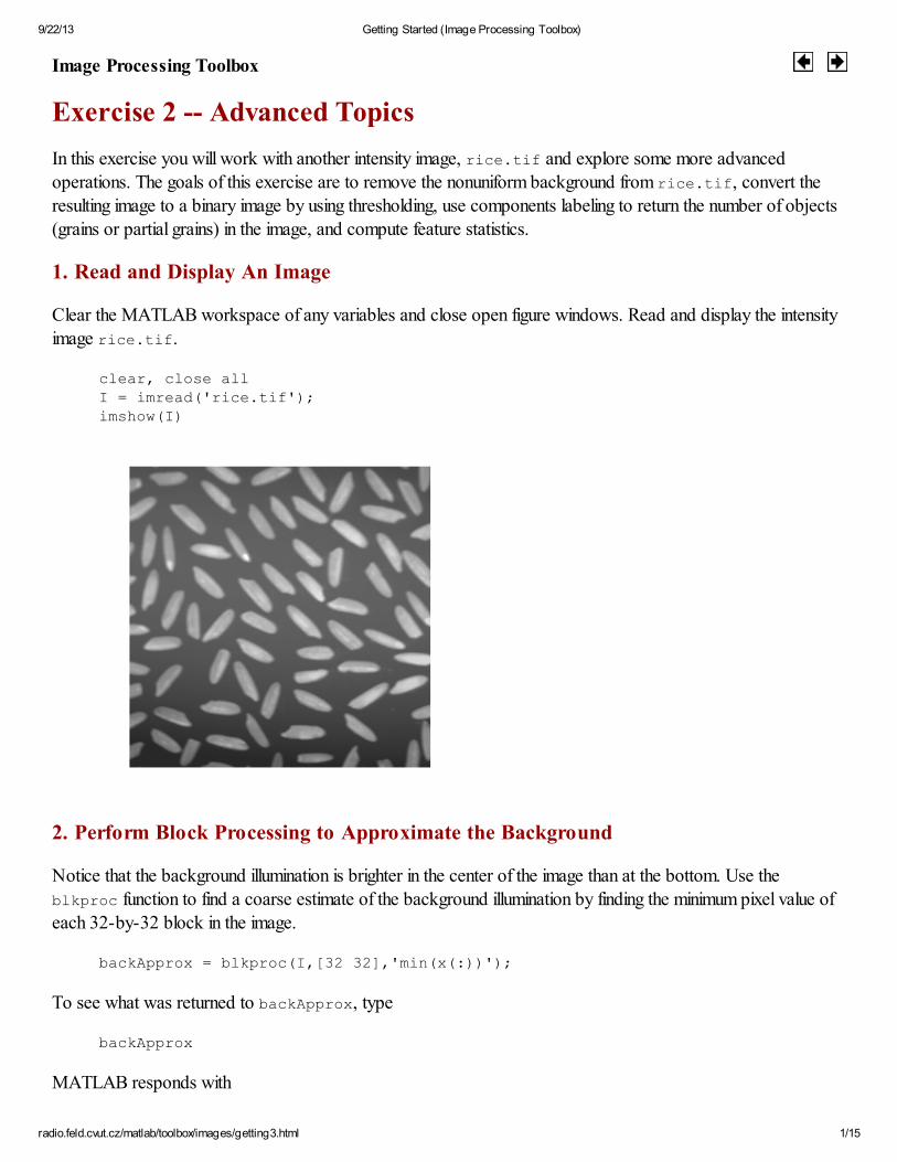
Clear the MATLAB workspace of any variables and close open figure windows. Read and display the intensity

image rice.tif.

clear, close allI = imread('rice.tif');imshow(I)

2. Perform Block Processing to Approximate the Background

Notice that the background illumination is brighter in the center of the image than at the bottom. Use the

blkproc function to find a coarse estimate of the background illumination by finding the minimum pixel value of

each 32-by-32 block in the image.

backApprox = blkproc(I,[32 32],'min(x(:))');

To see what was returned to backApprox, type

backApprox

MATLAB responds with

9/22/13 Getting Started (Image Processing Toolbox)

radio.feld.cvut.cz/matlab/toolbox/images/getting3.html 2/15

backApprox =

80 81 81 79 78 75 73 71 90 91 91 90 89 87 84 83 94 96 96 97 96 95 94 90 90 93 93 95 96 95 94 93 80 83 85 87 87 88 87 87 68 69 72 74 76 76 77 76 48 51 54 56 59 60 61 61 40 40 40 40 40 40 40 41

Here's What Just Happened

Step 1. You used the toolbox functions imread and imshow to read and display an 8-bit intensity

image. imread and imshow are discussed in Exercise 1, in 2. Check the Image in Memory, under the

"Here's What Just Happened" discussion.

Step 2. blkproc found the minimum value of each 32-by-32 block of I and returned an 8-by-8

matrix, backApprox. You called blkproc with an input image of I, and a vector of [32 32], which

means that I will be divided into 32-by-32 blocks. blkproc is an example of a "function function,"meaning that it enables you to supply your own function as an input argument. You can pass in the name

of an M-file, the variable name of an inline function, or a string containing an expression (this is themethod that you used above). The function defined in the string argument ('min(x(:))') tells

blkproc what operation to perform on each block. For detailed instructions on using functionfunctions, see Appendix A.

MATLAB's min function returns the minimum value of each column of the array within parentheses. Toget the minimum value of the entire block, use the notation (x(:)), which reshapes the entire block intoa single column. For more information, see min in the MATLAB Function Reference.

3. Display the Background Approximation As a Surface

Use the surf command to create a surface display of the background approximation, backApprox. surf

requires data of class double, however, so you first need to convert backApprox using the double command.You also need to divide the converted data by 255 to bring the pixel values into the proper range for an image ofclass double, [0 1].

backApprox = double(backApprox)/255; % Convert image to double.figure, surf(backApprox);

9/22/13 Getting Started (Image Processing Toolbox)

radio.feld.cvut.cz/matlab/toolbox/images/getting3.html 3/15

To see the other side of the surface, reverse the y-axis with this command,

set(gca,'ydir','reverse'); % Reverse the y-axis.

To rotate the surface in any direction, click on the rotate button in the toolbar (shown at left), then click

and drag the surface to the desired view.

Here's What Just Happened

Step 3. You used the surf command to examine the background image. The surf command creates colored

parametric surfaces that enable you to view mathematical functions over a rectangular region. In the first

surface display, [0, 0] represents the origin, or upper-left corner of the image. The highest part of the curve

indicates that the highest pixel values of backApprox (and consequently rice.tif) occur near the middle

9/22/13 Getting Started (Image Processing Toolbox)

radio.feld.cvut.cz/matlab/toolbox/images/getting3.html 4/15

rows of the image. The lowest pixel values occur at the bottom of the image and are represented in the surface

plot by the lowest part of the curve. Because the minimum intensity values in each block of this image make asmooth transition across the image, the surface is comprised of fairly smooth curves.

The surface plot is a Handle Graphics® object, and you can therefore fine-tune its appearance by setting

properties. ("Handle Graphics" is the name for the collection of low-level graphics commands that create theobjects you generate using MATLAB.) The call to reverse the y-axis is one of many property settings that youcan make. It was made using the set command, which is used to set all properties. In the line,

set(gca,'ydir','reverse');

gca refers to the handle of the current axes object and stands for "get current axes." You can also set manyproperties through the Property Editor. To invoke the Property Editor, open the figure window's Edit

menu, and select Figure Properties, Axes Properties, or Current Object Properties. To select an object

to modify with the Property Editor, click the property the following button on the figure window, , then

click on the object. You can also use the other buttons in the toolbar to add new text or line objects to your

figure.

For information on working with MATLAB graphics, see the MATLAB graphics documentation.

4. Resize the Background Approximation

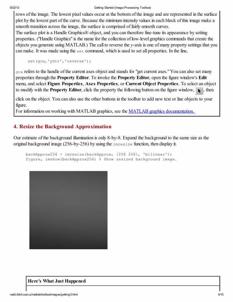
Our estimate of the background illumination is only 8-by-8. Expand the background to the same size as the

original background image (256-by-256) by using the imresize function, then display it.

backApprox256 = imresize(backApprox, [256 256], 'bilinear');figure, imshow(backApprox256) % Show resized background image.

Here's What Just Happened

9/22/13 Getting Started (Image Processing Toolbox)

radio.feld.cvut.cz/matlab/toolbox/images/getting3.html 5/15

Step 4. You used imresize with "bilinear" interpolation to resize your 8-by-8 background

approximation, backApprox, to an image of size 256-by-256, so that it is now the same size as

rice.tif. If you compare it to rice.tif you can see that it is a very good approximation. The goodapproximation is possible because of the low spatial frequency of the background. A high-frequency

background, such as a field of grass, could not have been as accurately approximated using so few

blocks.

The interpolation method that you choose for imresize determines the values for the new pixels you

add to backApprox when increasing its size. (Note that interpolation is also used to find the best values

for pixels when an image is decreased in size.) The other types of interpolation supported by imresizeare "nearest neighbor" (the default), and "bicubic." For more information on interpolation and resizing

operations, see Interpolation and Image Resizing.

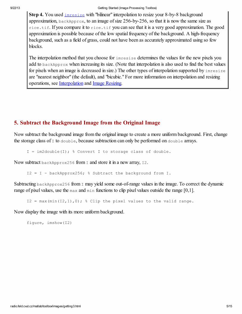
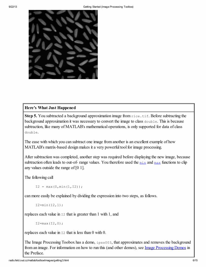
5. Subtract the Background Image from the Original Image

Now subtract the background image from the original image to create a more uniform background. First, change

the storage class of I to double, because subtraction can only be performed on double arrays.

I = im2double(I); % Convert I to storage class of double.

Now subtract backApprox256 from I and store it in a new array, I2.

I2 = I - backApprox256; % Subtract the background from I.

Subtracting backApprox256 from I may yield some out-of-range values in the image. To correct the dynamic

range of pixel values, use the max and min functions to clip pixel values outside the range [0,1].

I2 = max(min(I2,1),0); % Clip the pixel values to the valid range.

Now display the image with its more uniform background.

figure, imshow(I2)

9/22/13 Getting Started (Image Processing Toolbox)

radio.feld.cvut.cz/matlab/toolbox/images/getting3.html 6/15

Here's What Just Happened

Step 5. You subtracted a background approximation image from rice.tif. Before subtracting the

background approximation it was necessary to convert the image to class double. This is because

subtraction, like many of MATLAB's mathematical operations, is only supported for data of class

double.

The ease with which you can subtract one image from another is an excellent example of how

MATLAB's matrix-based design makes it a very powerful tool for image processing.

After subtraction was completed, another step was required before displaying the new image, because

subtraction often leads to out-of- range values. You therefore used the min and max functions to clipany values outside the range of [0 1].

The following call

I2 = max(0,min(1,I2));

can more easily be explained by dividing the expression into two steps, as follows.

I2=min(I2,1);

replaces each value in I2 that is greater than 1 with 1, and

I2=max(I2,0);

replaces each value in I2 that is less than 0 with 0.

The Image Processing Toobox has a demo, ipss003, that approximates and removes the background

from an image. For information on how to run this (and other demos), see Image Processing Demos in

the Preface.

9/22/13 Getting Started (Image Processing Toolbox)

radio.feld.cvut.cz/matlab/toolbox/images/getting3.html 7/15

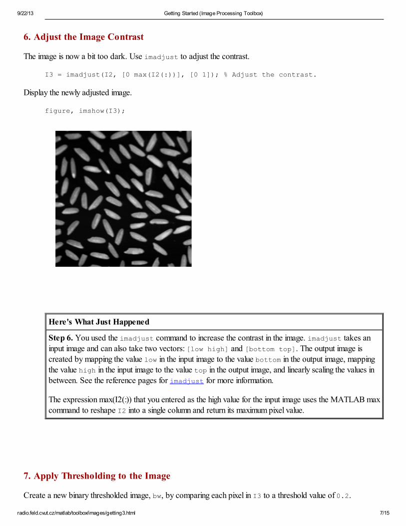
6. Adjust the Image Contrast

The image is now a bit too dark. Use imadjust to adjust the contrast.

I3 = imadjust(I2, [0 max(I2(:))], [0 1]); % Adjust the contrast.

Display the newly adjusted image.

figure, imshow(I3);

Here's What Just Happened

Step 6. You used the imadjust command to increase the contrast in the image. imadjust takes an

input image and can also take two vectors: [low high] and [bottom top]. The output image iscreated by mapping the value low in the input image to the value bottom in the output image, mapping

the value high in the input image to the value top in the output image, and linearly scaling the values in

between. See the reference pages for imadjust for more information.

The expression max(I2(:)) that you entered as the high value for the input image uses the MATLAB max

command to reshape I2 into a single column and return its maximum pixel value.

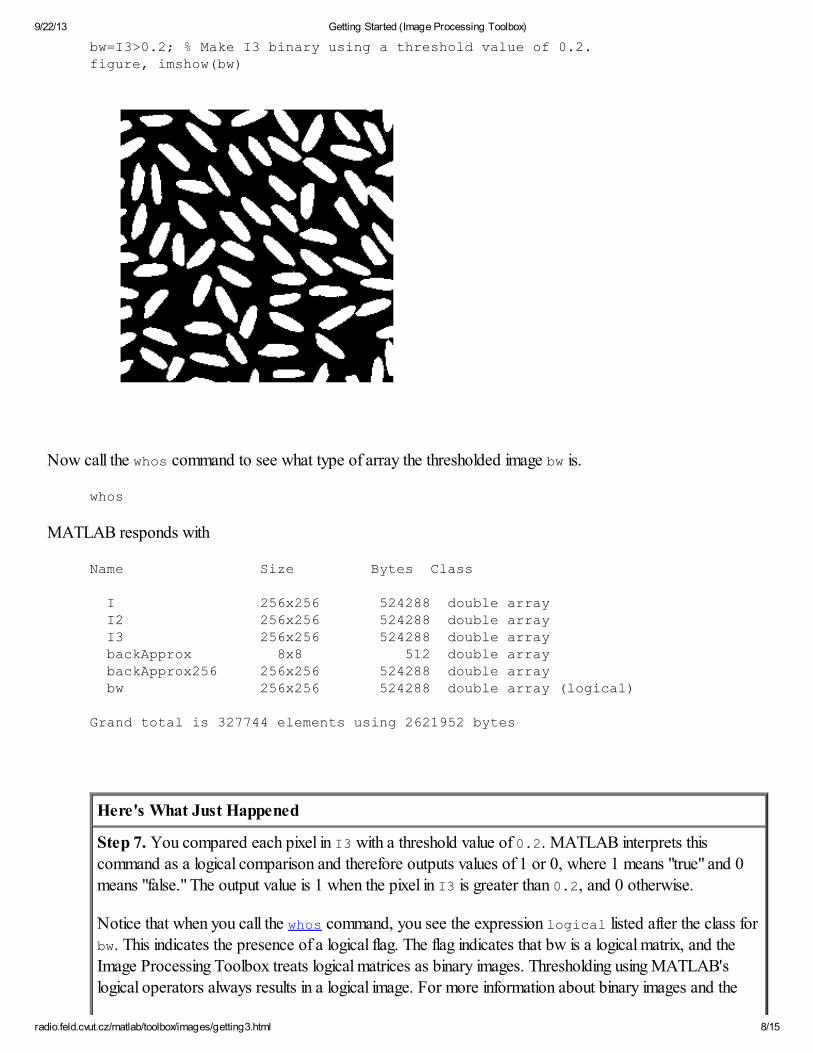
7. Apply Thresholding to the Image

Create a new binary thresholded image, bw, by comparing each pixel in I3 to a threshold value of 0.2.

9/22/13 Getting Started (Image Processing Toolbox)

radio.feld.cvut.cz/matlab/toolbox/images/getting3.html 8/15

bw=I3>0.2; % Make I3 binary using a threshold value of 0.2.figure, imshow(bw)

Now call the whos command to see what type of array the thresholded image bw is.

whos

MATLAB responds with

Name Size Bytes Class

I 256x256 524288 double array I2 256x256 524288 double array I3 256x256 524288 double array backApprox 8x8 512 double array backApprox256 256x256 524288 double array bw 256x256 524288 double array (logical)

Grand total is 327744 elements using 2621952 bytes

Here's What Just Happened

Step 7. You compared each pixel in I3 with a threshold value of 0.2. MATLAB interprets this

command as a logical comparison and therefore outputs values of 1 or 0, where 1 means "true" and 0means "false." The output value is 1 when the pixel in I3 is greater than 0.2, and 0 otherwise.

Notice that when you call the whos command, you see the expression logical listed after the class for

bw. This indicates the presence of a logical flag. The flag indicates that bw is a logical matrix, and the

Image Processing Toolbox treats logical matrices as binary images. Thresholding using MATLAB's

logical operators always results in a logical image. For more information about binary images and the

9/22/13 Getting Started (Image Processing Toolbox)

radio.feld.cvut.cz/matlab/toolbox/images/getting3.html 9/15

logical flag, see Binary Images.

Thresholding is the process of calculating each output pixel value based on a comparison of the

corresponding input pixel with a threshold value. When used to separate objects from a background,

you provide a threshold value over which a pixel is considered part of an object, and under which a

pixel is considered part of the background. Due to the uniformity of the background in I3 and its high

contrast with the objects in it, a fairly wide range of threshold values can produce a good separation of

the objects from the background. Experiment with other threshold values. Note that if your goal were tocalculate the area of the image that is made up of the objects, you would need to choose a more precise

threshold value -- one that would not allow the background to encroach upon (or "erode") the objects.

Note that the Image Processing Toolbox also supplies the function im2bw, which converts an RGB,

indexed, or intensity image to a binary image based on the threshold value that you supply. You could

have used this function in place of the MATLAB command, bw = I3 > 0.2. For example,

bw = im2bw(I3, 0.2). See the reference page for im2bw for more information.

8. Use Connected Components Labeling to Determine the Number of Objects in theImage

Use the bwlabel function to label all of the connected components in the binary image bw.

[labeled,numObjects] = bwlabel(bw,4);% Label components.

Show the number of objects found by bwlabel.

numObjects

MATLAB responds with

numObjects =

80

You have just calculated how many objects (grains or partial grains of rice) are in rice.tif.

Note The accuracy of your results depends on a number of factors, including:

· The size of the objects

· The accuracy of your approximated background

· Whether you set the connected components parameter to 4 or 8

· The value you choose for thresholding

· Whether or not any objects are touching (in which case they may be

labeled as one object)

9/22/13 Getting Started (Image Processing Toolbox)

radio.feld.cvut.cz/matlab/toolbox/images/getting3.html 10/15

In this case, some grains of rice are touching, so bwlabel treats them as one object.

To add some color to the figure, display labeled using a vibrant colormap created by the hot function.

map = hot(numObjects+1); % Create a colormap.imshow(labeled+1,map); % Offset indices to colormap by 1.

Here's What Just Happened

Step 8. You called bwlabel to search for connected components and label them with unique numbers.

bwlabel takes a binary input image and a value of 4 or 8 to specify the "connectivity" of objects. The

value 4, as used in this example, means that pixels that touch only at a corner are not considered to be

"connected." For more information about the connectivity of objects, see Connected-Components

Labeling.

A labeled image was returned in the form of an indexed image, where zeros represent the background,and the objects have pixel values other than zero (meaning that they are labeled). Each object is given a

unique number (you can see this when you go to the next step,9. Examine an Object). The pixel values

are indices into the colormap created by hot.

Your last call to imshow uses the syntax that is appropriate for indexed images, which is,

imshow(labeled+1, map);

Because labeled is an indexed image, and 0 is meaningless as an index into a colormap, a value of 1

was added to all pixels before display. The hot function creates a colormap of the size you specify. We

created a colormap with one more color than there are objects in the image because the first color is

used for the background. MATLAB has several colormap-creating functions, including gray, pink,

copper, and hsv. For information on these functions, see colormap in the MATLAB Function

9/22/13 Getting Started (Image Processing Toolbox)

radio.feld.cvut.cz/matlab/toolbox/images/getting3.html 11/15

Reference.

You can also return the number of objects by asking for the maximum pixel value in the image. For

example,

max(labeled(:))ans =

80

9. Examine an Object

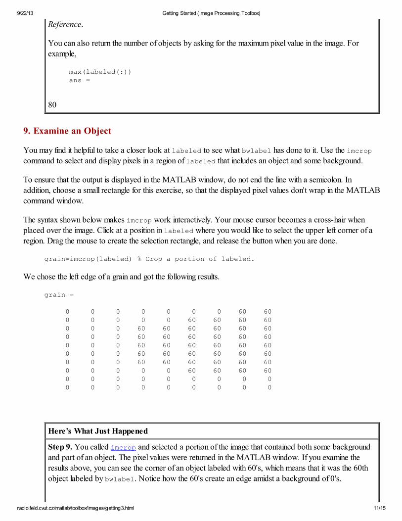
You may find it helpful to take a closer look at labeled to see what bwlabel has done to it. Use the imcropcommand to select and display pixels in a region of labeled that includes an object and some background.

To ensure that the output is displayed in the MATLAB window, do not end the line with a semicolon. In

addition, choose a small rectangle for this exercise, so that the displayed pixel values don't wrap in the MATLAB

command window.

The syntax shown below makes imcrop work interactively. Your mouse cursor becomes a cross-hair when

placed over the image. Click at a position in labeled where you would like to select the upper left corner of aregion. Drag the mouse to create the selection rectangle, and release the button when you are done.

grain=imcrop(labeled) % Crop a portion of labeled.

We chose the left edge of a grain and got the following results.

grain =

0 0 0 0 0 0 0 60 60 0 0 0 0 0 60 60 60 60 0 0 0 60 60 60 60 60 60 0 0 0 60 60 60 60 60 60 0 0 0 60 60 60 60 60 60 0 0 0 60 60 60 60 60 60 0 0 0 60 60 60 60 60 60 0 0 0 0 0 60 60 60 60 0 0 0 0 0 0 0 0 0 0 0 0 0 0 0 0 0 0

Here's What Just Happened

Step 9. You called imcrop and selected a portion of the image that contained both some background

and part of an object. The pixel values were returned in the MATLAB window. If you examine the

results above, you can see the corner of an object labeled with 60's, which means that it was the 60th

object labeled by bwlabel. Notice how the 60's create an edge amidst a background of 0's.

9/22/13 Getting Started (Image Processing Toolbox)

radio.feld.cvut.cz/matlab/toolbox/images/getting3.html 12/15

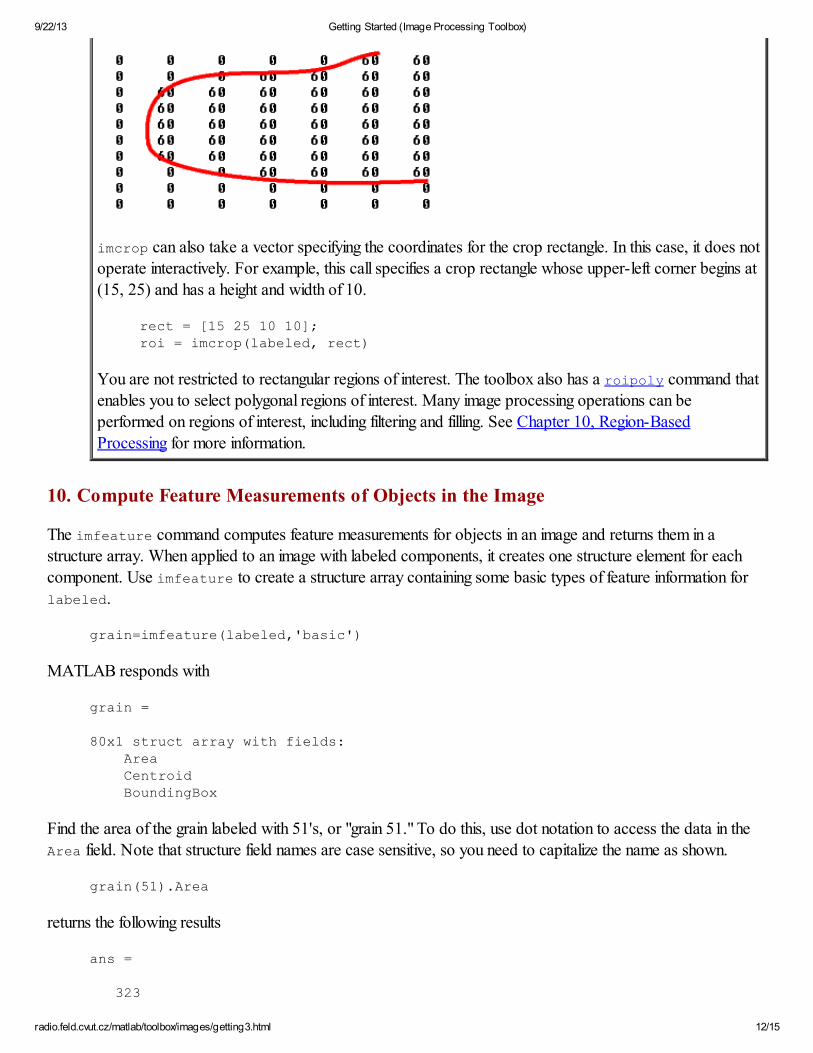
imcrop can also take a vector specifying the coordinates for the crop rectangle. In this case, it does notoperate interactively. For example, this call specifies a crop rectangle whose upper-left corner begins at

(15, 25) and has a height and width of 10.

rect = [15 25 10 10];roi = imcrop(labeled, rect)

You are not restricted to rectangular regions of interest. The toolbox also has a roipoly command thatenables you to select polygonal regions of interest. Many image processing operations can be

performed on regions of interest, including filtering and filling. See Chapter 10, Region-BasedProcessing for more information.

10. Compute Feature Measurements of Objects in the Image

The imfeature command computes feature measurements for objects in an image and returns them in astructure array. When applied to an image with labeled components, it creates one structure element for each

component. Use imfeature to create a structure array containing some basic types of feature information forlabeled.

grain=imfeature(labeled,'basic')

MATLAB responds with

grain =

80x1 struct array with fields: Area Centroid BoundingBox

Find the area of the grain labeled with 51's, or "grain 51." To do this, use dot notation to access the data in the

Area field. Note that structure field names are case sensitive, so you need to capitalize the name as shown.

grain(51).Area

returns the following results

ans =

323

9/22/13 Getting Started (Image Processing Toolbox)

radio.feld.cvut.cz/matlab/toolbox/images/getting3.html 13/15

Find the smallest possible bounding box and the centroid (center of mass) for grain 51.

grain(51).BoundingBox, grain(51).Centroid

returns

ans =

141.5000 89.5000 26.0000 27.0000ans =

155.3437 102.0898

Create a new vector, allgrains, which holds just the area measurement for each grain. Then call the whoscommand to see how allgrains is allocated in the MATLAB workspace.

allgrains=[grain.Area];whos allgrains

MATLAB responds with

Name Size Bytes Class

allgrains 1x80 640 double array

Grand total is 80 elements using 640 bytes

allgrains contains a one-row array of 80 elements, where each element contains the area measurement of agrain. Check the area of the 51st element of allgrains.

allgrains(51)

returns

ans =

323

which is the same result that you received when using dot notation to access the Area field of grains(51).

Here's What Just Happened

Step 10. You called imfeature to return a structure of basic feature measurements for each thresholded

grain of rice. imfeature supports many types of feature measurement, but setting the measurementsparameter to basic is a convenient way to return three of the most commonly used measurements: the area,

the centroid (or center of mass), and the bounding box. The bounding box represents the smallest rectanglethat can contain a region, or in this case, a grain. The four-element vector returned by the BoundingBox field,

[141.5000 89.5000 26.0000 27.0000]

shows that the upper left corner of the bounding box is positioned at [141.5 89.5], and the box has a width

of 26.0 and a height of 27.0. (The position is defined in spatial coordinates, hence the decimal values. For

9/22/13 Getting Started (Image Processing Toolbox)

radio.feld.cvut.cz/matlab/toolbox/images/getting3.html 14/15

more information on the spatial coordinate system, see Spatial Coordinates.) For more information about

working with MATLAB structure arrays, see Structures in the MATLAB graphics documentation.

You used dot notation to access the Area field of all of the elements of grain and stored this data to a newvector allgrains. This step simplifies analysis made on area measurements because you do not have to use

field names to access the area.

11. Compute Statistical Properties of Objects in the Image

Now use MATLAB functions to calculate some statistical properties of the thresholded objects. First use max to

find the size of the largest grain. (If you have followed all of the steps in this exercise, the "largest grain" is actuallytwo grains that are touching and have been labeled as one object).

max(allgrains)

returns

ans =

749

Use the find command to return the component label of this large-sized grain.

biggrain=find(allgrains==749)

returns

biggrain =

68

Find the mean grain size.

mean(allgrains)

returns

ans =

275.8250

Make a histogram containing 20 bins that show the distribution of rice grain sizes.

hist(allgrains,20)

9/22/13 Getting Started (Image Processing Toolbox)

radio.feld.cvut.cz/matlab/toolbox/images/getting3.html 15/15

Here's What Just Happened

Step 11. You used some of MATLAB's statistical functions, max, mean, and hist to return thestatistical properties for the thresholded objects in rice.tif.

The Image Processing Toolbox also has some statistical functions, such as mean2 and std2, which are

well suited to image data because they return a single value for two-dimensional data. The functionsmean and std were suitable here because the data in allgrains was one dimensional.

The histogram shows that the most common sizes for rice grains in this image are in the range of 300 to400 pixels.

Exercise 1 -- Some Basic Topics Where to Go From Here