Image Processing for Engineers by Andrew E. Yagle and Fawwaz T. Ulaby Solutions to the Exercises

Welcome message from author
This document is posted to help you gain knowledge. Please leave a comment to let me know what you think about it! Share it to your friends and learn new things together.
Transcript
Image Processing for Engineersby Andrew E. Yagle and Fawwaz T. Ulaby
Solutions to the Exercises
1

Chapter 1: Imaging Sensors
Chapter 2: Review of 1-D Signals and Systems
Chapter 3: 2-D Images and Systems
Chapter 4: Image Interpolation
Chapter 5: Image Enhancement
Chapter 6: Deterministic Approach to Image Restoration
Chapter 7: Wavelets and Compressed Sensing
Chapter 8: Random Variables, Processes, and Fields
Chapter 9: Stochastic Denoising and Deconvolution
Chapter 10: Color Image Processing
Chapter 11: Image Recognition
Chapter 12: Supervised Learning and Classification
2

Chapter 1Imaging Sensors
Exercises
1-1
1-2
1-3
1-4
3
Chapter 2Review of 1-D Signals and Systems
Exercises
2-1
2-2
2-3
2-4
2-5
2-6
2-7
2-8
2-9
2-10
2-11
2-12
2-13
4

Chapter 32-D Images and Systems
Exercises
3-1
3-2
3-3
3-4
3-5
3-6
3-7
3-8
3-9
3-10
3-11
3-12
3-13
3-14
3-15
5

Chapter 4Image Interpolation
Exercises
4-1
4-2
4-3
4-4
4-5
4-6
4-7
4-8
4-9
4-10
6

Chapter 5Image Enhancement
Exercises
5-1
5-2
5-3
5-4
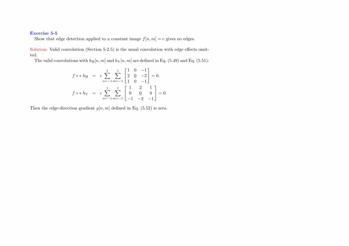
5-5
7

Chapter 6Deterministic Approach to Image Restoration
Exercises
6-1
6-2
8

Chapter 7Wavelets and Compressed Sensing
Exercises
7-1
7-2
7-3
7-4
7-5
7-6
7-7
7-8
7-9
9
Chapter 8Random Variables, Processes, and Fields
Exercises
8-1
8-2
8-3
8-4
8-5
8-6
8-7
8-8
8-9
8-10
8-11
8-12
8-13
10

Chapter 9Stochastic Denoising and Deconvolution
Exercises
9-1
9-2
9-3
9-4
9-5
9-6
9-7
9-8
9-9
9-10
9-11
9-12
9-13
11

Chapter 10Color Image Processing
Exercises
10-1
10-2
10-3
10-4
10-5
10-6
10-7
12

Chapter 11Image Recognition
Exercises
11-1
11-2
11-3
13

Chapter 12Supervised Learning and Classification
Exercises
12-1
12-2
14

Exercise 1-1An imaging lens used in a digital camera has a diameter of 25 mm and a focal length of
50 mm. Considering the photodetectors response to the red band centered at λ = 0.6 µm,what is the camera’s spatial resolution in the image plane, given that the image distancefrom the lens is di = 50.25 mm. What is the corresponding resolution in the object plane?
Solution: Image: ∆ymin = 1.47 µm. Object: ∆y′min = 0.3 mm.
Details:Using Eq. (1.1), 1
do+ 1di
= 1f becomes 1
do+ 1
50.25 mm = 150 mm , so do = 10050 mm = 10.05 m.
Using Eq. (1.9a), ∆ymin = 1.22diλD = 1.22(50.25 mm)0.6 µm
25 mm = 1.47 µm.Using Eq. (1.9b), ∆y′min = 1.22do
λD = 1.22(10050 mm)0.6 µm
25 mm = 0.3 mm.
15

Exercise 1-2At λ = 10 µm, what is the ratio of the emissivity of a snow-covered surfacerelative to that of a sand-covered surface? (See Fig. 1-14).
Solution: esnowesand
≈ 0.985/0.9 = 1.09.
Details: Examining Fig. 1-14 at wavelength 10 µm, snow/ice (the red curve) is 0.985 anddesert (the black curve) is 0.90.
16

Exercise 1-3With reference to the diagram Fig. 1-21, suppose the length of the real aperture `ywere to be increased from 2 m to 8 m. What would happen to (a) the antenna beamwidth,(b) length of the synthetic aperture, and (c) the SAR azimuth resolution?
Solution: (a) Beamwidth is reduced by a factor of 4, (b) synthetic aperture length is reducedfrom 8 km to 2 km, and (c) SAR azimuth resolution increases from 1 m to 4 m.
Details:(a) Using Eq. (1.12), real antenna beamwidth is ∆y′min = λ
`yR. Increasing `y decreases
∆y′min.(b) Using Eq. (1.13), increasing ` increases ∆y′min, equivalent to a shorter SAR length(c) Using Eq. (1.13), ∆y′min = `
2 = 2 m2 =1 m becomes 8 m
2 = 4 m.
17

Exercise 1-4A 6 MHz ultrasound system generates pulses with 2 cycles per pulse using a 5 cm × 5
cm 2-D transducer array. What are the dimensions of its resolvable voxel when focused ata range of 8 cm in a biological material?
Solution: ∆V = ∆Rmin ×∆xmin ×∆ymin = 0.26 mm×0.41 mm×0.41 mm.
Details:The wavelength of the pulses is λ = 1540 m/s
6 MHz = 0.257 mm.Using Eq. (1.22), ∆Rmin = λN
2 = 0.257 mm(2)2 = 0.257 mm.
Using Eq. (1.24), ∆xmin = RfλLx
= (8 cm)0.257 mm5cm = 0.41 mm. Similarly, ∆ymin = 0.41
mm.
18

Exercise 2-1Compute the value of
∫∞−∞ δ(3t− 6)t2 dt.
Solution: By the time-scaling property Eq. (2.6) of impulses, δ(3t− 6) = 13δ(t− 2).
By the sifting property Eq. (2.4) of impulses,∫∞−∞
13δ(t− 2)t2 dt = 1
322 = 43 .
So∫∞−∞ δ(3t− 6)t2 dt =
∫∞−∞
13δ(t− 2)t2 dt = 1
322 = 43 .
19

Exercise 2-2Compute the energy of the pulse defined by x(t) = 5 rect((t− 2)/6).
Solution: The energy E of x(t) is defined in Eq. (2.2) as E =∫∞−∞ |x(t)|2 dt.
rect(t) has support (is nonzero) −12 < t < 1
2 . rect(t/6) has support −3 ≤ t ≤ 3.x(t) has support −1 ≤ t ≤ 5. So the energy of x(t) is
E =∫ 5
−1|5|2 dt = 25(5− (−1)) = 150 .
20

Exercise 2-3Is the following system linear, time-invariant, both, or neither? dy
dt = 2x(t−1)+3tx(t+1).
Solution: A system is linear if it has the property for any constants ci and inputs xi(t),that:
If xi(t)→ SYSTEM → yi(t), then∑Ni=1 cixi(t)→ SYSTEM →
∑Ni=1 ciyi(t).
Substituting∑Ni=1 cixi(t) for x(t) and
∑Ni=1 ciyi(t) for y(t) gives
N∑i=1
cidyidt
= 2N∑i=1
cixi(t− 1) + 2tN∑i=1
cixi(t+ 1),
which is the linear combination∑Ni=1 ci of
dyidt
= 2xi(t− 1) + 3txi(t+ 1).
So the system is linear .
A system is time-invariant if it has the property, for any constant T , that:If x(t)→ SYSTEM → y(t), then x(t− T )→ SYSTEM → y(t− T ).Substituting x(t− T ) for x(t) and y(t− T ) for y(t) gives
dy(t− T )dt
= 2x(t− T − 1) + 3tx(t− T + 1),
which is not the original system with t replaced with t−T (the last term is 3tx(t−T + 1),not 3(t− T )x(t− T + 1)). So the system is not time-invariant .
21
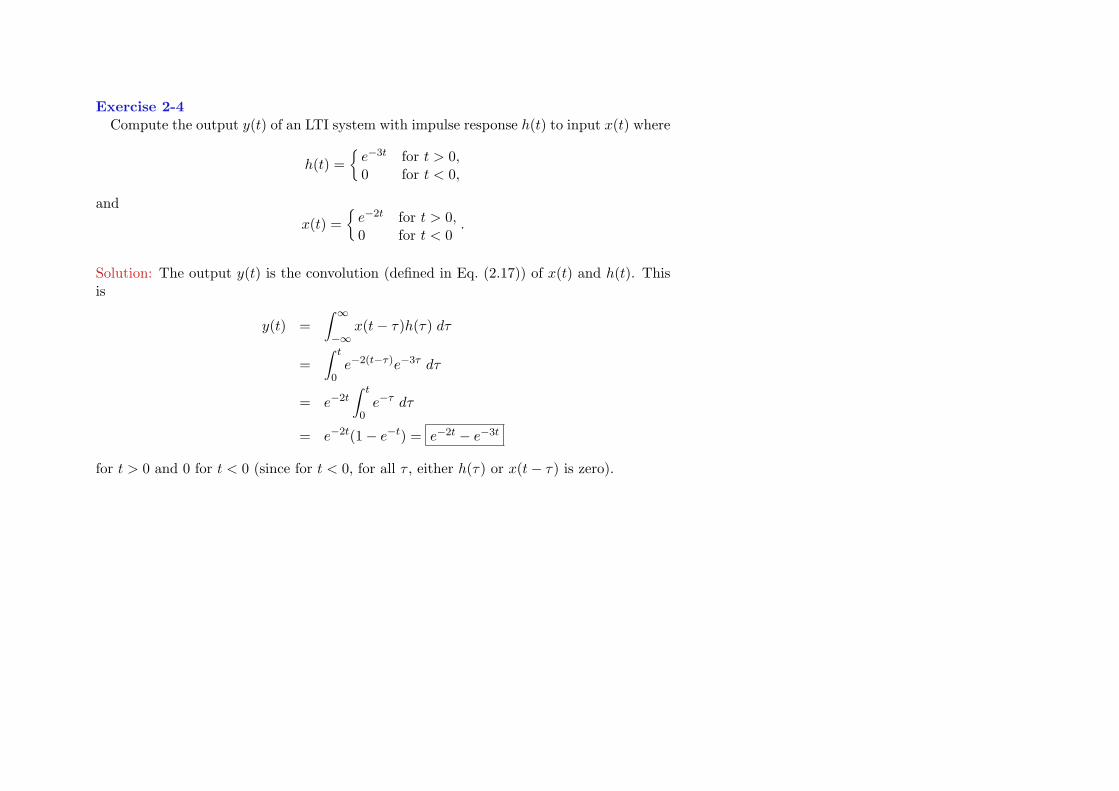
Exercise 2-4Compute the output y(t) of an LTI system with impulse response h(t) to input x(t) where
h(t) =e−3t for t > 0,0 for t < 0,
andx(t) =
e−2t for t > 0,0 for t < 0
.
Solution: The output y(t) is the convolution (defined in Eq. (2.17)) of x(t) and h(t). Thisis
y(t) =∫ ∞−∞
x(t− τ)h(τ) dτ
=∫ t
0e−2(t−τ)e−3τ dτ
= e−2t∫ t
0e−τ dτ
= e−2t(1− e−t) = e−2t − e−3t
for t > 0 and 0 for t < 0 (since for t < 0, for all τ , either h(τ) or x(t− τ) is zero).
22

Exercise 2-5A square wave x(t) has the Fourier series expansionx(t) = sin(t) + 1
3 sin(3t) + 15 sin(5t) + 1
7 sin(7t) + . . .
Compute output y(t) if x(t)→ h(t) = 0.4 sinc(0.4t) → y(t).
Solution: x(t) has components at 12π = 0.16 Hz, 3
2π = 0.48 Hz, 52π = 0.80 Hz, 7
2π = 1.12 Hz,. . .h(t) is the impulse response of an ideal lowpass filter Eq. (2.34) with cutoff frequency
fc = 0.2 Hz. Only the sinusoid at 0.2 Hz gets through the lowpass filter, so y(t) = sin(t)
23
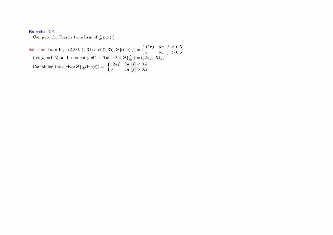
Exercise 2-6Compute the Fourier transform of d
dtsinc(t).
Solution: From Eqs. (2.33), (2.34) and (2.35), FFFsinc(t) =j2πf for |f | < 0.50 for |f | > 0.5
(set fc = 0.5), and from entry #5 in Table 2-4, FFFdxdt = (j2πf) X(f).
Combining these gives FFF ddtsinc(t) =j2πf for |f | < 0.50 for |f | > 0.5
24

Exercise 2-7What is the Nyquist sampling rate for a signal bandlimited to 4 kHz?
Solution: From Section 2-4.1, the Nyquist rate is 2(4 kHz) = 8000 samples/s .
25

Exercise 2-8A 500 Hz sinusoid is sampled at 900 samples/s. No anti-alias filter is being used.What is the frequency of the reconstructed continuous-time sinusoid?
Solution: The spectrum of the sampled signal has components at frequencies±500,±900± 500,±1800± 500, . . . = ±400,±500,±1300,±1400, . . . Hz.The reconstruction filter is a lowpass filter with cutoff 1
2(900) = 450 Hz.This leaves components at ±400 Hz. The frequency of the reconstructed sinusoid is
400 Hz .
26

Exercise 2-9A 28-Hertz sinusoid is sampled at 100 samples/second. What is Ω0 for the resulting
discrete-time sinusoid? What is the period of the resulting discrete-time sinusoid?
Solution: From Eq. (2.62), Ω0 = 2π 28100 = 0.56π From Eq. (2.63), Ω0
2π = 2π0.56π = N
D = 257 .
The period is the numerator N = 25Check: cos(0.56π[n+ 25]) = cos(0.56πn+ [0.56π25]) = cos(0.56πn+ 14π) = cos(0.56πn).
27

Exercise 2-10Compute the output y[n] of a discrete-time LTI system with impulse response h[n] and
input x[n], where h[n] = 3, 1 and x[n] = 1, 2, 3, 4.
Solution: From Eq. (2.71d), the output is the convolution y[n] = h[n] ∗ x[n] =(3)(1), (3)(2) + (1)(1), (3)(3) + (1)(2), (3)(4) + (1)(3), (1)(4) = 3, 7, 11, 15, 4
28

Exercise 2-11Compute the DTFT of 4 cos(0.15πn+ 1).
Solution: 4 cos(0.15πn+ 1) = 2ej1ej0.15πn + 2e−j1e−j0.15πn. Now take DTFTs of this.Applying the modulation property entry #3 in Table #2-6 to entry #2 in Table #2-7
givesDTFT[AejΩ0t] = A2πδ((Ω− Ω0)), where δ((Ω− Ω0)) =
∑∞k=−∞ δ(Ω− 2πk − Ω0).
Using this twice gives DTFT[4 cos(0.15πn+1)]=4πej1δ((Ω−0.15))+4πe−j1δ((Ω+0.15)).
29

Exercise 2-12Compute the inverse DTFT of 4 cos(2Ω) + 6 cos(Ω) + j8 sin(2Ω) + j2 sin(Ω).
Solution: Using 2 cos(Ω) = ejΩ + e−jΩ and 2j sin(Ω) = ejΩ − e−jΩ,we can rewrite this as 4 cos(2Ω) + 6 cos(Ω) + j8 sin(2Ω) + j2 sin(Ω)= 2[ej2Ω + e−j2Ω] + 3[ejΩ + e−jΩ] + 4[ej2Ω − e−j2Ω] + 1[ejΩ − e−jΩ]= (2 + 4)ej2Ω + (3 + 1)ej2Ω + (3− 1)e−jΩ + (2− 4)e−j2Ω = 6ej2ω + 4ej2ω + 2e−jω− 2e−j2ω.Using the definition Eq. (2.73a) of DTFT, we can read off the inverse DTFT asDTFT−1[4 cos(2Ω) + 6 cos(Ω) + j8 sin(2Ω) + j2 sin(Ω)] = 6, 4, 0, 2,−2.
30

Exercise 2-13Compute the 4-point DFT of 4, 3, 2, 1.
Solution: From Eq. (2.89a), the DFT is X[k] =∑N−1n=0 x[n] e−j2πnk/N for k = 0, 1, . . . , N−1.
Here N = 4 so X[k] =∑3n=0 x[n] e−j2πnk/4 for k = 0, 1, 2, 3.
Since e−j2πnk/4 = (e−j2π/4)nk = (−j)nk, this becomesX[0] = 1x[0] + 1x[1] + 1x[2] + 1x[3] since k = 0→ (−j)n0 = 1.X[1] = 1x[0]− jx[1]− 1x[2] + jx[3] since k = 1→ (−j)n1 = (−j)n.X[2] = 1x[0]− 1x[1] + 1x[2]− 1x[3] since k = 2→ (−j)n2 = (−1)n.X[3] = 1x[0] + jx[1]− 1x[2]− jx[3] since k = 3→ (−j)n3 = ((−j)3)n = jn.Inserting x[0] = 4, x[1] = 3, x[2] = 2, x[3] = 1 givesX[0] = 4 + 3 + 2 + 1 = 10 and X[1] = 4− j3− 2 + j1 = 2− j2.X[2] = 4− 3 + 2− 1 = 02 and X[3] = 4 + j3− 2− j1 = 2 + j2.DFT[4, 3, 2, 1]= 10, 2− j2, 2, 2 + j2 X[3] = X∗[1] as required by conjugate symme-
try.
31

Exercise 3-1How does one tell whether an image displayed in color is a color or a false-color image?
Solution: False-color images should have colorbars to identify the numerical value associatedwith each color.
32

Exercise 3-2Which of the following images is separable: (a) 2-D impulse; (b) box; (c) disk.
Solution: 2-D impulse δ(x, y) = δ(x) δ(y) and box Eq. (3.2) are separable; disk Eq. (3.3) isnot separable.
33

Exercise 3-3Which of the following is invariant to rotation: (a) 2-D impulse; (b) box; (c) disk.
Solution: 2-D impulse and disk are invariant to rotation; box is not invariant to rotation.
34

Exercise 3-4The operation of a 2-D mirror is described by g(x, y) = f(−x,−y). Find its PSF.
Solution: h(x, y; ξ, η) = δ(x+ ξ, y + η) This is a good example of a non-LSI system.The superposition integral Eq. (3.14) is
g(x, y) =∫ ∫
f(ξ, η) h(x, y; ξ, η) dξ dη.
We need to find h(x, y; ξ, η) so that
g(x, y) = f(−x,−y) =∫ ∫
f(ξ, η) h(x, y; ξ, η) dξ dη.
By inspection, h(x, y; ξ, η) = δ(x+ ξ, y + η) works.
35

Exercise 3-5If g(x, y) = h(x, y) ∗ ∗f(x, y), what is 4h(x, y) ∗ ∗f(x− 3, y − 2) in terms of g(x, y)?
Solution: 4g(x− 3, y − 2) by shift and scaling properties of 1-D convolution (Table 2-3).
36

Exercise 3-6Why do f(x, y) and f(x− x0, y − y0) have the same magnitude spectrum |F(µ, ν)|?
Solution: Let g(x, y) = f(x− x0, y − y0). Then, from entry #3 in Table 3-1,
|G(µ, ν)| = |e−j2πµx0e−j2πνy0F(µ, ν)| = |e−j2πµx0e−j2πνy0 |F(µ, ν)| = |F(µ, ν)|.
37
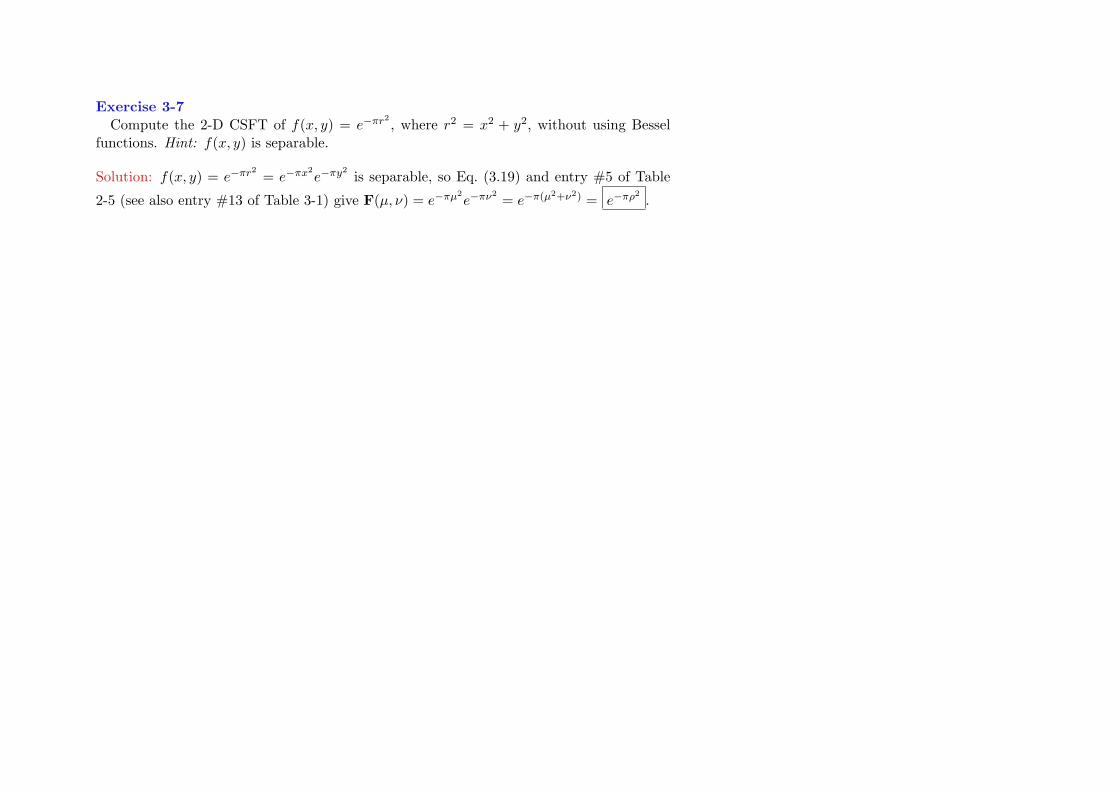
Exercise 3-7Compute the 2-D CSFT of f(x, y) = e−πr
2, where r2 = x2 + y2, without using Bessel
functions. Hint: f(x, y) is separable.
Solution: f(x, y) = e−πr2
= e−πx2e−πy
2is separable, so Eq. (3.19) and entry #5 of Table
2-5 (see also entry #13 of Table 3-1) give F(µ, ν) = e−πµ2e−πν
2= e−π(µ2+ν2) = e−πρ
2.
38

Exercise 3-8The 1-D phase spectrum φ(µ) in Fig. 3-6(c) is either 0 or 180 for all µ. Yet the phase
of the 1-D CTFT of a real-valued function must be an odd function of frequency. How canthese two statements be reconciled?
Solution: A phase of 180 is equivalent to a phase of −180. Replacing 180 with −180
for µ < 0 in Fig. 3-6(c) makes the phase φ(µ) an odd function of µ.
39

Exercise 3-9An image is spatially bandlimited to 10 cycles/m in both x and y directions. What is
the minimum sampling length ∆s to avoid aliasing?
Solution: ∆s < 12B = 1
20m . This is the sampling theorem (see Sections 2-4 and 3-5).
40

Exercise 3-10The 2-D CSFT of a 2-D impulse is one, so it is not spatially bandlimited. Why is it
possible to sample an impulse?
Solution: In general, it isn’t. Using a sampling interval of ∆s, the impulse δ(x−x0, y− y0)will be missed unless x0 and y0 are both integer multiples of ∆s.
41
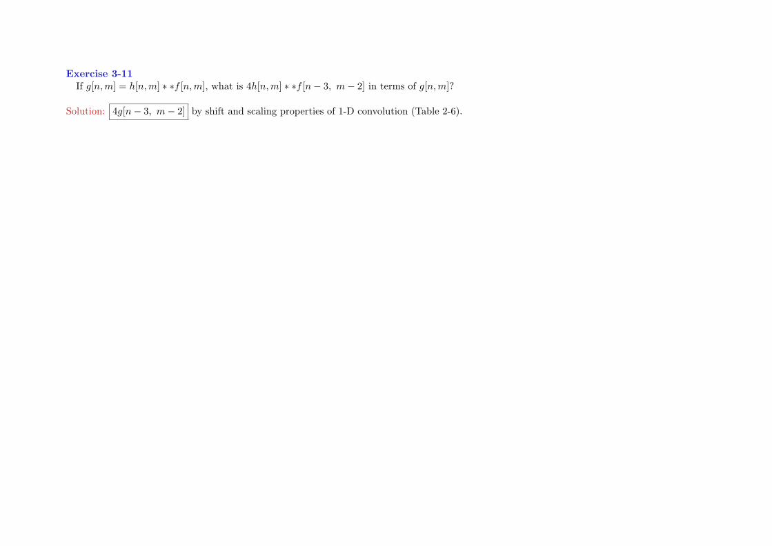
Exercise 3-11If g[n,m] = h[n,m] ∗ ∗f [n,m], what is 4h[n,m] ∗ ∗f [n− 3, m− 2] in terms of g[n,m]?
Solution: 4g[n− 3, m− 2] by shift and scaling properties of 1-D convolution (Table 2-6).
42
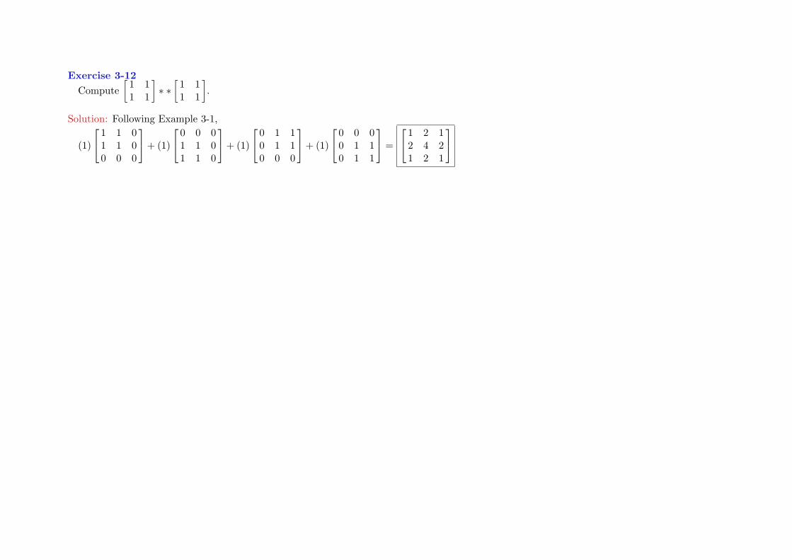
Exercise 3-12Compute
[1 11 1
]∗ ∗[
1 11 1
].
Solution: Following Example 3-1,
(1)
1 1 01 1 00 0 0
+ (1)
0 0 01 1 01 1 0
+ (1)
0 1 10 1 10 0 0
+ (1)
0 0 00 1 10 1 1
=
1 2 12 4 21 2 1
43
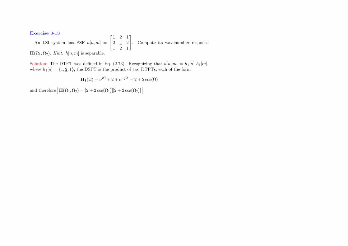
Exercise 3-13
An LSI system has PSF h[n,m] =
1 2 12 4 21 2 1
. Compute its wavenumber response
H(Ω1,Ω2). Hint: h[n,m] is separable.
Solution: The DTFT was defined in Eq. (2.73). Recognizing that h[n,m] = h1[n] h1[m],where h1[n] = 1, 2, 1, the DSFT is the product of two DTFTs, each of the form
H1(Ω) = ejΩ + 2 + e−jΩ = 2 + 2 cos(Ω)
and therefore H(Ω1,Ω2) = [2 + 2 cos(Ω1)][2 + 2 cos(Ω2)] .
44
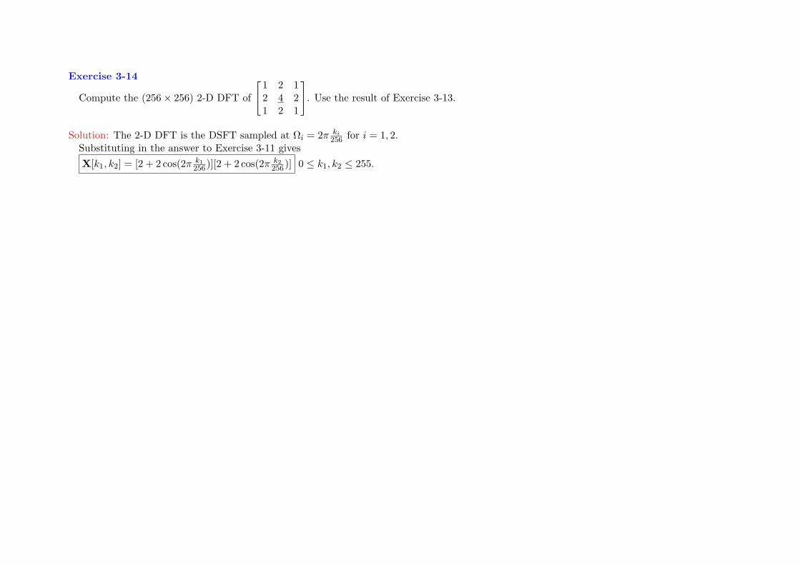
Exercise 3-14
Compute the (256× 256) 2-D DFT of
1 2 12 4 21 2 1
. Use the result of Exercise 3-13.
Solution: The 2-D DFT is the DSFT sampled at Ωi = 2π ki256 for i = 1, 2.
Substituting in the answer to Exercise 3-11 givesX[k1, k2] = [2 + 2 cos(2π k1
256)][2 + 2 cos(2π k2256)] 0 ≤ k1, k2 ≤ 255.
45

Exercise 3-15Why did this book not spend more space on computing the DSFT?
Solution: Because in practice, the DSFT is computed using the 2-D DFT.
46

Exercise 4-1If sinc interpolation is applied to the samples x(0.1n) = cos(2π(6)0.1n), what will be
the result?
Solution: x(0.1n) are samples of a 6 Hz cosine sampled at a rate of 10 samples/second.Sinc interpolation will be a cosine with frequency aliased to (10 − 6) = 4 Hz (see Section2-4.3).
47

Exercise 4-2Upsample the length-2 signal x[n] = 8, 4 to a length-4 signal y[n].
Solution: The 2-point DFT X[k] = 8 + 4, 8− 4 = 12, 4. Since N = 2 is even, we split4 and insert a zero in the middle, to get Y[k] = 12, 2, 0, 2. The inverse 4-point DFT is
y[0] =14
(12 + 2 + 0 + 2) = 4,
y[1] =14
(12 + 2j − 0− 2j) = 3,
y[2] =14
(12− 2 + 0− 2) = 2,
y[3] =14
(12− 2j + 0 + 2j) = 3.
Multiplying by 42 gives y[n] = 8, 6, 4, 6
48

Exercise 4-3Show that the area under βN (t) is one.
Solution:∫∞−∞ βN (t) dt = B(0) by entry #11 in Table 2-4.
Now set f = 0 in sincN (f) and use sinc(0)=1.
49

Exercise 4-4Why does βN (t) look like a Gaussian function for N ≥ 3?
Solution: Because βN (t) is rect(t) convolved with itself N+1 times. By the central limittheorem of probability, convolving any square-integrable function with itself results in afunction resembling a Gaussian.
50

Exercise 4-5Show that the support of βN (t) is −N+1
2 < t < N+12 .
Solution: The support of βN (t) is the interval outside of which βN (t) = 0. The support ofrect(t) is −1
2 < t < 12 . βN (t) is rect(t) convolved with itself N +1 times, which has duration
N + 1 centered at t = 0.
51

Exercise 4-6Given the samples x(0), x(∆), x(2∆), x(3∆) = 7, 4, 3, 2, compute x(∆/3) by interpo-
lation using: (a) nearest neighbor; (b) linear.
Solution: (a) ∆/3 is closer to 0 than to ∆, so x(∆/3) = x(0) = 7 .(b) x(∆/3) = 2
3x(0) + 13x(∆) = 2
3(7) + 13(4) = 6 .
52

Exercise 4-7In Eq. (4.63), why isn’t c[n] = x(n∆) for N ≥ 2?Answer: Because 3 of the basis functions βN
(t∆ −m
)overlap for any t. See Fig. 4-11.
53

Exercise 4-8The “image”
[1 23 4
]is interpolated using bilinear interpolation. What is the interpolated
value at the center of the image?
Solution: 14(1 + 2 + 3 + 4) = 2.5 .
54

Exercise 4-9The “image”
[1 23 4
]is rotated counter-clockwise 90. What is the result?
Solution:[
2 41 3
]This is pretty obvious.
55

Exercise 4-10The “image”
[4 812 16
]is magnified by a factor of three. What is the result, using: (a)
NN; (b) bilinear interpolation.
Solution: (a)
4 4 4 8 8 84 4 4 8 8 84 4 4 8 8 812 12 12 16 16 1612 12 12 16 16 1612 12 12 16 16 16
; (b)
1 2 1 2 4 22 4 2 4 8 41 2 1 2 4 23 6 3 4 8 46 12 6 8 16 83 6 3 4 8 4
.
Each of the 4 pixels of the original image is now the center of a (3× 3) array.
56

Exercise 5-1A star of magnitude six is barely visible to the naked eye in a dark sky. How much fainter
is a star of magnitude 6 than Vega, which has magnitude zero?
Solution: From Eq. (5.7), 106/2.512 = 244.6, so magnitude 6 is 245 times fainter than Vega.
57

Exercise 5-2What is another name for gamma transformation with γ = 1?
Solution: Linear transformation. Compare Eq. (5.10) and Eq. (5.1).
58
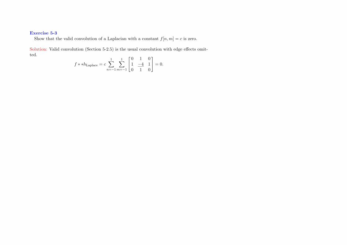
Exercise 5-3Show that the valid convolution of a Laplacian with a constant f [n,m] = c is zero.
Solution: Valid convolution (Section 5-2.5) is the usual convolution with edge effects omit-ted.
f ∗ ∗hLaplace = c1∑
n=−1
1∑m=−1
0 1 01 −4 10 1 0
= 0.
59

Exercise 5-4Perform histogram equalization on the (2× 2) “image”
[0.3 0.20.2 0.3
].
Solution: The histogram of the image is: 0.2 occurring twice and 0.3 occurring twice.The CDF is:
Pf (f0) =
0 for 0 ≤ f0 < 0.2,2 for 0.2 ≤ f0 < 0.3,4 for 0.3 ≤ f0 < 1.
Pixel value 0.2 is mapped to Pf (0.2) = 2 and pixel value 0.3 is mapped to Pf (0.3) = 4.
The histogram-equalized “image” is[
4 22 4
], which has a wider range of values than the
original.
60
Exercise 5-5Show that edge detection applied to a constant image f [n,m] = c gives no edges.
Solution: Valid convolution (Section 5-2.5) is the usual convolution with edge effects omit-ted.
The valid convolutions with hH[n,m] and hV[n,m] are defined in Eq. (5.49) and Eq. (5.51):
f ∗ ∗ hH = c1∑
n=−1
1∑m=−1
1 0 −12 0 −21 0 −1
= 0.
f ∗ ∗ hV = c1∑
n=−1
1∑m=−1
1 2 10 0 0−1 −2 −1
= 0.
Then the edge-direction gradient g[n,m] defined in Eq. (5.52) is zero.
61

Exercise 6-1Apply Tikhonov regularization with λ = 0.01 to the 1-D deconvolution problem x[0], x[1]∗h[0], h[1], h[2] = 2,−5, 4,−1, where h[0] = h[2] = 1 and h[1] = −2.
Solution: H(0) = 1− 2 + 1 = 0 so X(Ω) = Y(Ω)H(Ω) won’t work at Ω = 0, for any DFT order.
ButX(Ω) =
H∗(Ω)|H(Ω)|2 + λ2
Y(Ω)
does work.Using 4-point DFTs (computable by hand) gives
x[n] = 1.75,−1.25,−0.25,−0.25 ,
which is close to the actual x[n] = 2,−1. MATLAB:h=[1 -2 1];x=[2 -1];y=conv(x,h);H=fft(h,4);Y=fft(y);Z=conj(H).*Y./(abs(H).*abs(H)+0.0001);z=real(ifft2(Z)) provides the estimated
x[n].
62

Exercise 6-2For motion blur with a PSF of length N+1=60 in the direction of motion, at what spatial
frequencies Ω will the spatial frequency response be zero?
Solution: From Eq. (6.50), the numerator of the spatial frequency response is zero whenΩ = ±kπ/30 for any nonzero integer k.
63

Exercise 7-1(a) An input signal of duration N is fed into a tree-based filter bank of five stages. What
is the combined total duration of the output signals? Repeat for (b) an octave-based filterbank.
Solution: (a) 25N = 32N . (b) N since lower-wavenumber bands can be sampled less often.
64

Exercise 7-2A square wave x(t) has the Fourier series expansion x(t) =
∑∞k=1
1k sin(2πkt). x(t) is
passed through a brick-wall lowpass filter with cutoff frequency 2.5 Hz. What is the ratioof the average power of y(t) to the average power of x(t). Hint:
∑∞k=1
1k2 = π2
6 .
Solution: Rayleigh’s theorem relates average power to Fourier series coefficients.The average power of x(t) is
∑∞k=1
1k2 = π2
6 and the average power of y(t) is∑2k=1
1k2 =
1.25,since the lowpass filter has set the Fourier series coefficients for k ≥ 3 to zero.
1.25π2/6
= 0.76 .
65

Exercise 7-3Compute the cyclic convolution of 1, 2 and 3, 4 for N = 2.
Solution: Following Example 7-1, 1, 2 ∗ 3, 4 = 3, 10, 8. Aliasing gives 8 + 3, 10 =11, 10
66

Exercise 7-4x[n]→ ↑ 2 → ↓ 2 → y[n]. Express y[n] in terms of x[n].
Solution: y[n] = x[n] Zero-stuffing inserts zeros between consecutive values of x[n] anddecimating removes those zeros, leaving the original x[n].
67
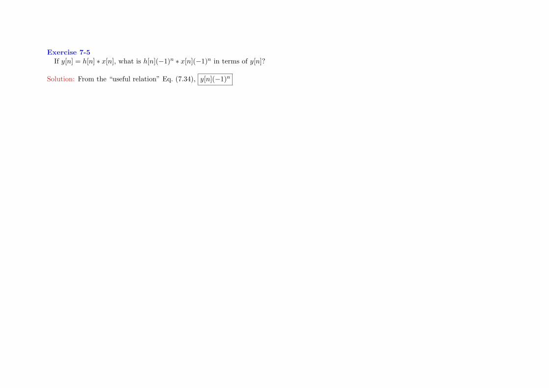
Exercise 7-5If y[n] = h[n] ∗ x[n], what is h[n](−1)n ∗ x[n](−1)n in terms of y[n]?
Solution: From the “useful relation” Eq. (7.34), y[n](−1)n
68

Exercise 7-6Compute the one-stage Haar transform of x[n] =
√24, 3, 3, 4.
Solution: x[n] c© 1√2[1, 1] = 8, 7, 6, 7. Hence, xLD[n] = 8, 6 .
x[n] c© 1√2[1,−1] = 0,−1, 0, 1. Hence, xHD[n] = 0, 0 .
69

Exercise 7-7If h[n] = 1
5√
26, 2, h[2], 3, find h[2] so that h[n] satisfies the Smith-Barnwell condition.
Solution: According to Eq. (7.63), the Smith-Barnwell condition requires the autocorrela-tion of h[n] to be 1 for n = 0 and to be 0 for even n 6= 0.
For h[n] = a, b, c, d, these conditions give a2 + b2 + c2 + d2 = 1, ac+bd = 0, andh[2] = −1
70

Exercise 7-8What are the finest-detail signals of the db3 wavelet transform of x[n] = 3n2?
Solution: Zero. db3 wavelet basis function h[n] eliminates quadratic signals by construction.
71

Exercise 7-9Show by direct computation that the db2 scaling function listed in Table 7-3 satisfies the
Smith-Barnwell condition.
Solution: The Smith-Barnwell condition requires the autocorrelation of g[n] to be 1 for n = 0and to be 0 for even n 6= 0. For g[n] = a, b, c, d these conditions give a2 + b2 + c2 + d2 = 1and ac+bd = 0. The db2 g[n] listed in Table 7-3 is g[n] = 0.4830, 0.8365, [0.2241,−[0.1294.
It is easily verified that the sum of the squares of these numbers is 1, and that (0.4830)×(0.2241) + (0.8365)× (−0.1294) = 0.
72

Exercise 8-1For the coin flip experiment, what is the pmf for n = # flips of all tails followed by the
first head?
Solution: p[n] = a(1− a)(n−1) since we require n−1 consecutive tails before the first head.This is called a geometric pmf.
73

Exercise 8-2Given that the result of the coin flip experiment for N = 2 was one head and one tail,
compute P[H1].
Solution: There are 2 ways of getting one head and one tail: H1T2 and T1H2.Let P[Hi] = a so that P[Ti] = 1− a, and events B = H1 and C = H1T2 ∪ T1H2.Then B ∩ C = H1T2 and P[H1|H1T2 ∪ T1H2] = P[B|C] = P[B∩C]
P[C] = a(1−a)a(1−a)+a(1−a) = 1
2 .
74
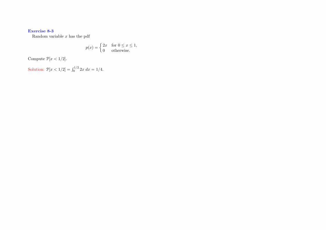
Exercise 8-3Random variable x has the pdf
p(x) =
2x for 0 ≤ x ≤ 1,0 otherwise.
Compute P[x < 1/2].
Solution: P[x < 1/2] =∫ 1/2
0 2x dx = 1/4.
75

Exercise 8-4Random variable n has the pmf p[n] = (1
2)n for integers n ≥ 1. Compute P[n ≤ 5].
Solution: P[n ≤ 5] =∑5n=1(1
2)n = 31/32.
76

Exercise 8-5 In Example 8-6, compute the marginal pdf p(y) and conditional marginalpdf p(x|y).
Solution:p(y) =
∫ y
02 dx =
2y for 0 ≤ y ≤ 1,0 otherwise.
p(x|y) =p(x, y)p(y)
=
22y for 0 ≤ x < y ≤ 1,0 otherwise.
As expected, this becomes an impulse if y = 0.
77

Exercise 8-6In Example 8-7, compute the marginal pmf p[m] and conditional marginal pmf p[n|m].
Solution: p[m] =∑mn′=0
16 =
1/6 for m = 0,2/6 for m = 1,3/6 for m = 2.
Hence p[m] = m+16 for m = 0,1,2. p[n|m] = p[n,m]
p[m] = 1/6(m+1)/6 = 1
m+1 for m = 0,1,2, whichsums to 1.
78

Exercise 8-7In Example 8-6, compute (a) the mean E(y) and (b) variance σ2
y .
Solution: (a)
p(y) =∫ y
02 dx =
2y for 0 ≤ y ≤ 1,0 otherwise.
E[y] =∫ 1
0 y(2y) dy = 2/3
(b) E[y2] =∫ 1
0 y2(2y) dy = 1/2. Hence σ2
y = 12 − (2
3)2 = 118
79
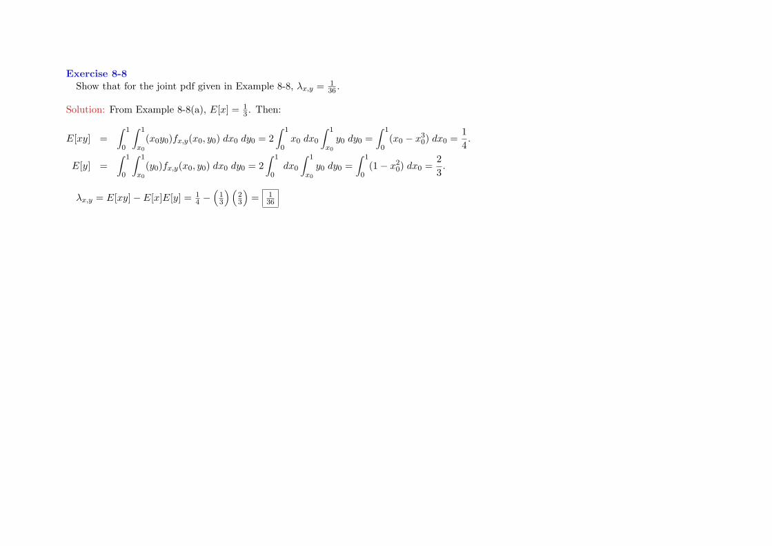
Exercise 8-8Show that for the joint pdf given in Example 8-8, λx,y = 1
36 .
Solution: From Example 8-8(a), E[x] = 13 . Then:
E[xy] =∫ 1
0
∫ 1
x0
(x0y0)fx,y(x0, y0) dx0 dy0 = 2∫ 1
0x0 dx0
∫ 1
x0
y0 dy0 =∫ 1
0(x0 − x3
0) dx0 =14.
E[y] =∫ 1
0
∫ 1
x0
(y0)fx,y(x0, y0) dx0 dy0 = 2∫ 1
0dx0
∫ 1
x0
y0 dy0 =∫ 1
0(1− x2
0) dx0 =23.
λx,y = E[xy]− E[x]E[y] = 14 −
(13
) (23
)= 1
36
80
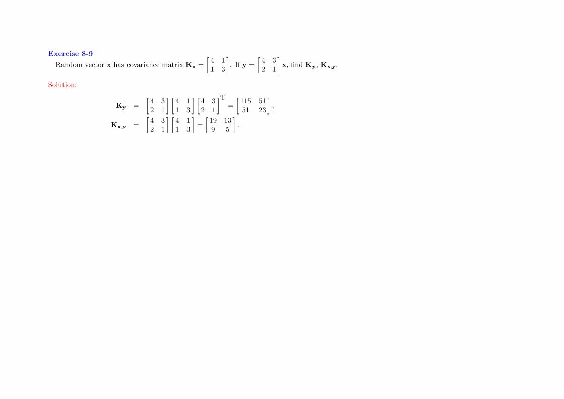
Exercise 8-9Random vector x has covariance matrix Kx =
[4 11 3
]. If y =
[4 32 1
]x, find Ky, Kx,y.
Solution:
Ky =[
4 32 1
] [4 11 3
] [4 32 1
]T=[
115 5151 23
],
Kx,y =[
4 32 1
] [4 11 3
]=[
19 139 5
].
81

Exercise 8-10A zero-mean WSS random process has power spectral density Sx(f) = 4
(2πf)2+4. What
is its autocorrelation function?
Solution: R(τ) = FFF−1Sx(f). From entry #3 in Table 2-5, R(τ) = e−2|τ |
82

Exercise 8-11A zero-mean WSS random process has the Gaussian autocorrelation function
R(τ) = e−πτ2.
What is its power spectral density?
Solution: Sx(f) = FFFR(τ). From entry #6 in Table 2-5, Sx(f) = e−πf2
83
Exercise 8-12x(t) is a white process with Rx(τ) = 5δ(τ) and y(t) =
∫ t+1t−1 x(τ) dτ , Compute the power
spectral density of y(t).
Solution: y(t) = rect(t/2) ∗ x(t). From entry #3 in Table #2-5, H(f) = FFFrect(t/2) =2 sinc(2f). So Sy(f) = |H(f)|2Sx(f) = 5(2 sinc(2f))2 = 20 sinc2(2f)
84

Exercise 8-13A white random field f(x, y) with auto-correlation function Rf (x, y) = 2δ(x) δ(y) is
filtered by an LSI system with PSF h(r) = 1r , where r is the radius in (x, y) space. Compute
the power spectral density of the output random field g(x, y).
Solution: From entry #5 in Table #3-2, H(ρ) = FFFh(r) = FFF1r = 1
ρ . Sf (µ, ν) = 2.
So Sg(µ, ν) = 2|H(ρ)|2 = 2ρ2
= 2µ2+ν2
85

Exercise 9-1How does Eq. (9.18) simplify when random vectors x and y are replaced with random
variables x and y?
Solution:xLS = x+
λx,yσ2y
(yobs − y).
Cross-covariance matrix Kx,y becomes covariance λx,y and covariance matrix Kx becomesvariance σ2
y .
86

Exercise 9-2Determine xLS and xMAP, given that only the a priori pdf p(x) is known.
Solution: xLS = x and xMAP = value of x maximizing p(x) .
Details:From Eq. (9.8), xLS = E[x|y = yobs ] = E[x] = x. p(yobs |x) is unknown since the
observation yobs is unknown. From Eq. (9.5), xMAP is the value of x maximizing p(x).
87

Exercise 9-3We observe random variable y whose pdf is p(y|λ) = λe−λy for y > 0. Compute the
maximum likelihood estimate of λ.
Solution: The log-likelihood function is log p(y|λ) = log λ− λyobs.
Setting its derivative to zero gives 1λ − yobs = 0. Solving, λMLE(yobs) =
1yobs
.
88

Exercise 9-4We observe random variable y whose pdf is p(y|λ) = λe−λy for y > 0 and λ has the a
priori pdf p(λ) = 3λ2 for 0 ≤ λ ≤ 1. Compute the maximum a posteriori estimate of λ.
Solution: The a posteriori pdf is
p(λ|y) =p(yobs|λ)p(λ)
p(yobs)= λe−λyobs
3λ2
p(yobs).
Its log is log λ − λyobs + log(3) + 2 log λ − log(p(yobs)). Setting its derivative to 0 gives3λ − yobs = 0.
Solving, λMAP(yobs) = 3/yobs if 3/yobs < 1, since λ < 1. Note λMAP(yobs) = 3λMLE(yobs).
89

Exercise 9-5Compute the MAP estimator for the coin-flip experiment assuming the a priori uniform
pdf p(x) = 1 for 0 ≤ x ≤ 1.
Solution: The algebra is the same as for computing xMLE. So xMAP = xMLE = nobs/N .
90

Exercise 9-6Compute the MAP estimator for the coin-flip experiment with N = 10 and the a priori
pdf p(x) = 3x2 for 0 ≤ x ≤ 1.
Solution: The a posteriori pdf is, modifying Eq. (9.28),
p(x|nobs) =3x2
C
xnobs(1− x)N−nobsN !
nobs!(N − nobs)!.
Taking the logarithm and omitting all terms independent of x gives
log p(x|nobs) = (nobs + 2) log x+ (N − nobs) log(1− x).
Setting the derivative to zero gives
0 =nobs + 2
x− N − nobs
1− x.
Solving for x gives
xMAP =nobs + 2N + 2
=nobs + 2
12.
91

Exercise 9-7Compute the MAP estimator for the coin-flip experiment with a triangular a priori pdf
p(x) = 2(1− x) for 0 ≤ x ≤ 1.
Solution: The a posteriori pdf is, modifying Eq. (9.28),
p(x|nobs) =2(1− x)
C
xnobs(1− x)N−nobsN !
nobs!(N − nobs)!.
Taking the logarithm and omitting all terms independent of x gives
log p(x|nobs) = (nobs) log x+ (N − nobs + 1) log(1− x).
Setting its derivative to zero gives
0 =nobs
x− N − nobs + 1
1− x.
Solving for x gives xMAP =nobs
N + 1.
Note that xMAP(nobs) < xMLE(nobs) as x is likely to be small, from the triangular a prioripdf.
92
Exercise 9-8Compute the mean and variance of the sample mean of N IID random variables xi,
each of which has mean x and variance σ2x.
Solution: From Chapter 8, the variance of the sum of uncorrelated random variables is thesum of their variances; independent random variables are uncorrelated, and σ2
ax = a2σ2x.
Let µ = 1N
∑Ni=1 xi be the sample mean of the xi. Then
σ2µ =
1N2
Nσ2x =
σ2x
M.
Also, E[µ] = 1N
∑Ni=1E[xi] = x, so the sample mean is an unbiased estimator of x.
So the sample mean converges to the actual mean x of the xi as M →∞.This is why the sample mean is useful, and why polling works.
93

Exercise 9-9What is MAP sparsifying estimator when noise variance σ2
v is much smaller than σx?
Solution: When σ2v σx, λ → 0 and xMAP = yobs from Eq. (9.82). This makes sense: if
the noise is low, use the observations whether or not they are a sparse estimate.
94

Exercise 9-10What is MAP sparsifying estimator when noise variance σ2
v is much greater than σx?
Solution: When σ2v σx, λ→∞, and xMAP = 0 from Eq. (9.82). This makes sense: the a
priori information that x is sparse dominates the noisy observation.
95

Exercise 9-11What happens to the stochastic Wiener filter when the observation noise σ2
v → 0?
Solution: In Eq. (9.93), letting σ2v → 0 results in RS(Ω) = Y(Ω)(1 − e−jΩ) whose inverse
DTFT is rs[n] = y[n]− y[n− 1] which is (noise-free) Eq. (9.84b).
96

Exercise 9-12When σf →∞, the Laplacian pdf given by Eq. (9.114) approaches the uniform distribu-
tion. What does the MAP estimate reduce to when σf →∞?
Solution: As σf →∞, λ→ 0, in which case fMAP[n,m]→ gobs[n,m] from Eq. (9.116).This makes sense: σf →∞ means the a priori sparseness information no longer holds,so we have no choice but to rely on the observation gobs[n,m].
97
Exercise 9-13Suppose we estimate the autocorrelation function Rx[n] of data x[n], n = 0, . . . , N − 1
using the sample mean over i of x[i] x[i− n], zero-padding x[n] as needed. Show thatthe DFT of Rx[n] is the periodogram (this is one reason why the periodogram works).
Solution:
Rx[n] =1N
N−1∑i=0
x[i] x[i− n] =1N
N−1∑i=0
x[i] x[−(n− i)] =1N
(x[n] ∗ x[−n]).
From entries #4 and #6 of Table 2-7, the DSFT of (x[n] ∗ x[−n]) is
X(Ω) X(−Ω) = X(Ω) X∗(Ω) = |X(Ω)|2,
which is the periodogram defined in Eq. (9.118) (recall that Ω is sampled at Ω = 2πk/N).
98

Exercise 10-1What should the output of imagesc(ones(3,3,3)) be?
Solution: A 3× 3 all white image (the combination of 3× 3 red, green and blue images).
99

Exercise 10-2An image has fR[n,m] = fG[n,m] = fB[n,m] = 1 for all [n,m]. What is its YIQ color
system representation?
Solution: fY[n,m] = 1 and fI[n,m] = fQ[n,m] = 0 for all [n,m], as discussed belowEq. (10.4).
100

Exercise 10-3Should gamma transformation be applied to images using the RGB or YIQ format?
Solution: YIQ format, because gamma transformation is nonlinear; applying it to an RGBimage would distort its colors.
101

Exercise 10-4Should linear transformation be applied to images using the RGB or YIQ format?
Solution: RGB format, since this is the color system used to display the transformed image.Linear transformation of YIQ images may result in gR[n,m], gG[n,m], gB[n,m] ≥ gmax inEq. (5.1), even though a linear transformation of linear transformation Eq. (5.1) is linear.
102

Exercise 10-5Can the colors of a deconvolved image differ from those of the original image?
Solution: Yes. Regularization can alter values of the reconstructed fR[n,m], gG[n,m],fB[n,m] image, and this will affect the colors. However, the effect is usually too slight tobe noticeable.
103

Exercise 10-6If the PSFs for different colors are different, can we still deconvolve the image?
Solution: Yes. Use the proper PSF for each color in Eq. (10.15).
104

Exercise 10-7If the length of the blur were N + 1 = 6, at what Ω1 values would H(Ω1,Ω2) = 0?
Solution: The numerator of Eq. (10.17) is zero when sin(Ω1(N + 1)/2) = 0, which occurswhen Ω1(N + 1)/2 is a multiple of π, or equivalently, when Ω1 = ±kπ/3 for integers k.
105

Exercise 11-1We have two classes of (1 × 1) images f1[n,m] = 1 and f2[n,m] = 4. Use correlation to
classify gobs[n,m] = 2.
Solution: ρ1 = (2)(1) = 2 and ρ2 = (2)(4) = 8. Since ρ2 > ρ1, classify gobs[n,m] as k = 2 .This is counter-intuitive (2 is closer to 1 than to 4), so see Exercise 11-2.
106

Exercise 11-2We have two classes of (1 × 1) images f1[n,m] = 1 and f2[n,m] = 4. Use the MLE
classifier to classify gobs[n,m] = 2.
Solution: ρ1 = (2)(1)=2 and ρ2 = (2)(4)=8. ΛMLE[1] = 2(2)−12 = 3 and ΛMLE[2] =2(8)−42 = 0. Since ΛMLE[1] > ΛMLE[2], classify gobs[n,m] as k = 1 .
Including energies of the images resulted in a different, and more intuitive, classification.
107

Exercise 11-3We have two classes of (1 × 1) images f1[n,m] = 1 and f2[n,m] = 4, with respective a
priori probabilities p[k = 1] = 0.1 and p[k = 2] = 0.9. The additive noise has σ2v = 3. Use
the MAP classifier to classify gobs[n,m] = 2.
Solution: ρ1 = (2)(1)=2 and ρ2 = (2)(4)=8.ΛMAP[1] = 2(2)−12+2(3) log(0.1) = −10.8.ΛMAP[2] = 2(4)−42+2(3) log(0.9) = −0.63.Since ΛMAP[2] > ΛMAP[1], classify gobs[n,m] as k = 2 .The a priori probabilities biased the classification towards k = 2.
108

Exercise 12-1Use a perceptron to implement a digital OR logic gate (y = x1 + x2, except 1 + 1 = 1).
Solution: Use Fig. 12-1(a) with φ(x) ≈ u(x), weights w1 = w2 = 1, and any w0 such that−1 < w0 < 0.
109

Exercise 12-2Use a perceptron to implement a digital AND logic gate (y = x1x2).
Solution: Use Fig. 12-1(a) with φ(x) ≈ u(x), weights w1 = w2 = 1, and any w0 such that−2 < w0 < −1.
110
Related Documents