Image Panoramic Mosaics: Stitching and Aligning a Whole View

Image Panoramic Mosaics: Stitching and Aligning a Whole View

CS585 Project – Final Report

Ziliang ZHU U54653575 Siyang LI U24843027 Yuqi GUO U84243487

[email protected] [email protected] [email protected]

1 Introduction

Image Panoramic Mosaics Generation, or photo stitching, is the process of combining multiple

photographic images with overlapping fields of view to produce a segmented panorama or high-

resolution image. With a set of images with contents of close views, algorithms are designed to

assemble them in proper geographical positions, close the gaps and cover the overlaps through rotation,

translation and zooming and eliminate negative visual effects with refinement.

As early as the 1990s, pioneering studies have demonstrated good result with long sequence of images.

The problem is further studied in the field of computer vision, image processing, etc. Recent research

proposes methods that better compensate for the flaws remaining and appearing in image stitching

process. The result of stitching serves in visual perception related industries such as Augmented Reality

(AR), photographing, expedition, etc.

In this project, we review and comprehend the fundamental method of panoramic mosaic generation,

identify outstanding algorithms and implementations, test and evaluate their abilities, and discuss

possible future works.

2 Related Works

The fundamental research we are referencing is [1], in which paper a 3-step image stitching method is

introduced. Starting from a rough image assembling, two phases of alignments reduce the gaps between

overlapping neighbors and the blur and ‘ghosting’ to generate optimized result. The recent works on the

panoramic generation problem extends and improves the steps originated from [1] and will be

evaluated in the project. The result is satisfactory; however, several problems remain. The blur effect is

reduced yet existent in difficult cases. The iterative local optimization needs hyper-parameter

surveillance. There are also areas of mosaics where the visual effect differs from its surroundings due to

optical distortion.

The studies introduced in [2] differs from [1] in the way that they attempt to accurately align the images

throughout the overlap area before compositing to achieve a so-called perfect alignment. Specifically, in

correspondence to poor regions, they propose a correspondence insertion algorithm such that a good

warping function can still be estimated.

The works of Zaragoza et al. offers a different strategy in the ‘deghosting’ step. Instead of relying on a

projective model (which is often inadequate) and then fix the resulting errors, [3] proposes to adjust the

model based on the data to improve the fitness. It is achieved by their as-projective-as-possible warps,

i.e., warps that aim to be globally projective, yet allow local deviations to account for model inadequacy.

They claim to be able to deal with more than a pure rotation in the images.

As-Natural-As-Possible method proposed in [4] encounters the perspective distortion that occurs in

stitching as follows: they linearize the homography in the regions that do not overlap with any other

image, then automatically estimate a global similarity transform using a subset of corresponding points

in the overlapping regions. Finally, interpolate smoothly between the homography and the global

similarity in the overlapping regions, and similarly extrapolate using the linearized homography (affine)

and the global similarity transform in the non-overlapping regions to generate a stitching result with

more ‘natural’ visual effect.

Scale-Invariant Feature Transform (SIFT) is a method designed as early as 2004 in [14] while its ability in

image stitching discussed frequently recently. The chief advance lies in novel steps as keypoint

localization and discarding.

Bay et al. present in [15] Speed-Up Robust Features (SURF) algorithm that outperforms precedented

detection methods with less consumption and more robustness. Building on the essence of previous

image feature detectors and descriptions, SURF achieves superior performance with a novel

combination of detection, description and matching.

3 Methods

3.1 Alignment Framework

The method presented is the fundamental work in image stitching, comprehending of which leads to the

evaluation and discussion of relatively modern approaches

The image mosaics are rendered as collections of images with associated geometrical transformations in

3D setting. We use a hierarchical motion estimation framework consisting of four parts: pyramid

construction, motion estimation, image warping and coarse-to-fine refinement.

For a camera centered at the origin, we can calculate its 3D location in the setting by converting image

coordinates 𝑥 = (𝑥, 𝑦, 1) to a 3D point 𝑝 = (𝑋, 𝑌, 𝑍) through formula:

𝑝 ∼ 𝑅−1𝑉−1𝑥

where 𝑅 is the 3D rotation matrices and 𝑉 = [𝑓 0 00 𝑓 00 0 1

] is the focal length scaling. The 𝑇in this formula

representing image plane translation that is 𝑇 = [1 0 𝑐𝑥

0 1 𝑐𝑦

0 0 1

] is omitted because we are assuming that

pixels are numbered so that the origin is at the image center, i.e., 𝑐𝑥 = 𝑐𝑦 = 0, allowing T to be

removed from the formula.

For a camera rotating around its center of projection, the mapping (perspective projection) between

two images 𝑘 and 𝑙 is:

𝑀 ～ 𝑉𝑘𝑅𝑘𝑅𝑙−1 𝑉𝑙

−1 , where each image is represented by 𝑉𝑘𝑅𝑘, i.e. a focal length and a 3D rotation.

We assume 𝑉 is known and 𝑉𝑘 = 𝑉 for all images for simplicity.

We update 𝑅𝑘 incrementally based on angular velocity 𝛺 = (𝑤𝑥 , 𝑤𝑦, 𝑤𝑧):

𝑅𝑘 = �̂�(𝛺)𝑅𝐾

or 𝑀 ← 𝑉�̂�(𝛺)𝑅𝑘𝑅𝑙−1𝑉−1

Keeping only terms linear in Omega, we simplify the above formula to:

𝑀′ ≈ 𝑉[𝐼 + 𝑋(𝛺)]𝑅𝑘𝑅𝑙−1 𝑉−1 = (𝐼 + 𝐷𝛺) 𝑀

Where 𝐷𝛺 = 𝑉𝑋(𝛺)𝑉−1 = [

0 −𝜔𝑧 𝑓𝜔𝑦 𝜔𝑧

𝜔𝑧 0 −𝑓𝜔𝑥

−𝜔𝑦/𝑓 𝜔𝑥/𝑓 0 ] is the deformation matrix, and X is the cross

product operator.

Computing the Jacobian of 𝐷𝛺 with respect to 𝛺 and applying the chain rule, we get new Jacobian:

𝐽𝛺 =𝜕𝑥′′

𝜕𝑑

𝜕𝑑

𝜕𝛺= [

−𝑥𝑦/𝑓 𝑓 + 𝑥2/𝑓 −𝑦

−𝑓 − 𝑦2/𝑓 𝑥𝑦/𝑓 𝑥 ]

𝑇

This Jacobian is then plugged into the previous incremental update formula, after which 𝑅𝑘can be

updated. It can be used to directly improve the current motion estimate by first computing local

intensity errors and gradients, and then accumulating the entries in the parameter gradient vector and

Hessian matrix. The resulting image however is usually defected in two aspects: being susceptible to

local minima and outliers and calculation inefficiency. The image will be refined and with two steps of

alignment.

3.2 Global Alignment

The previous approach suffers from accumulated misregistration errors for long image sequences. The

new global alignment method reduces the previous error by minimizing the misregistration between

overlap pairs of images.

The global alignment is a feature-based technique. One way to formulate the global alignment is to

minimize the difference between overlapping pairs of images, but it’s hard to compute. A simpler

formulation is to minimize the difference between the ray direction of corresponding points. The

advantage of this problem is that both pose and structure can be solved independently for each frame.

In order to formulate global alignment, it’s not necessary to explicitly recover the ray directions. We can

reformulate block adjustment to minimize over pose({𝑅𝑘 , 𝑓𝑘}) by using gradient descent method for all

frames. More specifically, we estimate the pose by minimizing the difference in ray directions between

all pairs of overlapping images. 𝐸({𝑅𝑘 , 𝑓𝑘}) is given by

∑ ‖𝑝𝑗𝑘 − 𝑝𝑗𝑙‖2

= ∑ ‖𝑅𝑘−1�̂�𝑗𝑘 − 𝑅𝑙

−1�̂�𝑗𝑙‖2

𝑗,𝑘,𝑙∈𝒩𝑗𝑘𝑗,𝑘,𝑙∈𝒩𝑗𝑘

Then, we can compute the estimated directions 𝑝𝑗 using the known correspondence from all

overlapping frames 𝒩𝑗𝑘 where the feature point 𝑗 is visible,

𝑝𝑗~1

𝑛𝑗𝑘 + 1∑ 𝑅𝑙

−1𝑉𝑙−1𝑥𝑗𝑙

𝑙∈𝒩𝑗𝑘∪𝑘

By applying the global alignment method, it simultaneously adjusts all frame rotations and computes a

new estimated focal length.

3.3 Local Alignment

As we model the images to be taken by parallax-free camera, the deviations result in local mis-

registrations. The deviations are sourced from camera translation, radial distortion, changing optical

centers and moving objects. Local alignment (deghosting) is the method to eliminate the resulting

‘ghosting’ (double images) and potential blur.

There are precedential methods to tackle the problem. For instance, we can choose one image as a base

and calculate the relative optical flow. This does not suit our task in which scenario the large mosaics

containing a sequence of considerable number of images. It is also possible to compute camera motion

and parallax explicitly, but it would not solve the biases from other sources. We desire the images in this

project to be globally consistent without assigned base. The local alignment approach that best fits our

destination is to calculate pair-wise flow between images followed by inferring local warps. By repeating

the local alignment method iteratively, it also reduces the effect of radial distortion in pioneering

studies.

The block adjustment algorithm described above generates 𝑝𝑗, a direction corresponding to the 𝑗-th

patch center in the 𝑘-th image, 𝑥𝑗𝑘. 𝑝𝑗 then is projected onto image 𝑘 as:

�̅�𝑗𝑘~𝑉𝑘𝑅𝑘

1

𝑛𝑗𝑘 + 1∑ 𝑅𝑙

−1𝑉𝑙−1𝑥𝑗𝑙

𝑙∈Njk∪𝑘

=1

𝑛𝑗𝑘 + 1(𝑥𝑗𝑘 + ∑ �̃�𝑗𝑙

𝑙∈𝑁𝑗𝑘

)

which can be converted into a motion estimate

�̅�𝑗𝑘 = �̅�𝑗𝑘 − 𝑥𝑗𝑘 =1

𝑛𝑗𝑘 + 1∑ 𝑢𝑗𝑙

𝑙∈𝑁𝑗𝑘

We understand this formula as that to bring patch center 𝑗 in image 𝑘 to the global registration frame,

the motion required is the average of the pairwise motion estimates of the images overlapping with it,

weighted by 𝑛𝑗𝑘

𝑛𝑗𝑘+1. The weight can be interpreted as the motion apportioned to the neighbors among

the union of the neighbors and image 𝑘 itself, so as to prevent overfitting, the situation where images

simply fit to each other but not meeting half-ways.

After calculating the local motion, we use inverse mapping algorithm to warp the images reducing the

‘ghosting’ effect. The algorithm takes the negative of the computed flow −�̅�𝑗𝑘 and apply a bilinear

function over the flow samples.

3.4 Scale-invariant feature transform

3.4.1 Scale-space extrema detection

At this stage, the main point of interest detection is the key point in SIFT architecture. The images are

convolved with Gaussian filters at different scales, and then continuous Gaussian blur is used to blur the

image differences to find the key points. The key point is according to the maximum and minimum of

the difference of Gaussian (DoG) at different scales. In other words, the 𝐷(𝑥, 𝑦, 𝜎) of the DoG image is

caused by

D(x, y, σ) = L(x, y, ki𝜎) − L(𝑥, y, kjσ)

L (x, y, kσ) is from the original image and Gaussian blur 𝐺 (𝑥, 𝑦, 𝑘𝜎) to convolute under the condition of

𝑘𝜎 scale., for example:

𝐿(𝑥, 𝑦, 𝜎) = 𝐺(𝑥, 𝑦, 𝑘𝑖𝜎) ∗ 𝐼(𝑥, 𝑦)

Once the DoG image is obtained, the maximum and minimum values in the DoG image can be found as

key points. In order to determine the key points, each pixel in the DoG image will be made with eight

pixels around the center of itself, and nine pixels in the same position of the adjacent scale

magnification in the same group of DoG images, a total of 26 points For comparison, if this pixel is the

maximum and minimum of these twenty-six pixels, then this pixel is called a key point.

3.4.2 Keypoint localization

Too many key points may be found in different size spaces, and some key points may be relatively

difficult to identify or susceptible to noise interference. The next step of the SIFT algorithm will locate

each key point by the information of the pixels near the key point, the size of the key point, and the

main curvature of the key point, thereby eliminating the key points that are located on the side or are

susceptible to noise interference

3.4.3 Interpolation of nearby data for accurate position

For each possible key point, interpolating neighboring data can determine its position. The initial

method is to record the position and scale of each key point in the picture.

The newly developed method points out that the calculation of extremely worthwhile positions can

provide more accurate and reliable matching. This method uses the second Taylor series of DoG images

𝐷(𝑥, 𝑦, 𝜎) and uses the key point as the origin. Its expansion can be written as:

𝑫(𝐱) = 𝑫 +𝝏𝑫𝑻

𝝏𝒙𝒙 +

𝟏

𝟐

𝝏𝟐𝑫

𝝏𝒙𝟐 𝒙

The value of D and its partial differential is determined by the position of the key point, the variable 𝑥 =

(𝑥, 𝑦, 𝜎) is the offset to this key point.

3.4.4 Discarding low-contrast keypoints

This step will calculate the value of 𝑥 of the above quadratic Taylor series 𝐷(𝑥). If this value is less than

0.03, this key point is discarded. Otherwise, keep this key point and record its location as 𝑦 + 𝑥, where y

is the position of the key point at the beginning.

3.4.5 Eliminating edge responses

The DoG function is quite sensitive to the detection of points on edge. Even if it finds that the key points

located on edge are susceptible to noise, they will be detected as key points. Therefore, in order to

increase the reliability of key points, it is necessary to eliminate the key points that have high edge

response but whose position is not good enough.

3.4.6 Orientation assignment

In the orientation assignment, the key point uses the gradient direction distribution of adjacent pixels as

the specified direction parameter, so that the key point descriptor can be expressed according to this

direction and has rotation invariance.

Gaussian Blurred Image𝐿(𝑥, 𝑦, 𝜎), under 𝜎 size Gradient 𝑚(𝑥, 𝑦) and direction 𝜃(𝑥, 𝑦) can be calculated

from adjacent pixel values:

𝑚(𝑥, 𝑦) = √((𝐿(𝑥 + 1, 𝑦) − 𝐿(𝑥 − 1, 𝑦))2

+ ((𝐿(𝑥, 𝑦 + 1) − 𝐿(𝑥, 𝑦 − 1))2

𝜃(𝑥, 𝑦) = 𝑎𝑟𝑐𝑡𝑎𝑛 ((𝐿(𝑥, 𝑦 − 1) − 𝐿(𝑥, 𝑦 + 1))/(𝐿(𝑥 − 1, 𝑦) − 𝐿(𝑥 + 1, 𝑦)))

After calculating the magnitude and direction of the gradient of each key point and its neighboring

pixels, a 36 histogram in units of 10 degrees is established for it. Each adjacent pixel is added to the

histogram of key points according to its magnitude and direction, and finally, the direction of the

maximum value in the histogram is the direction of this key point. If the difference between the

maximum value and the local maximum value is within 20%, this key point is judged to contain multiple

directions, so an additional key point with the same position and different direction will be established.

3.4.7 Keypoint descriptor

After finding the position and size of the key point and giving the key point direction, it will ensure the

invariance of its movement, scaling, and rotation. In addition, it is necessary to establish a descriptor

vector for key points, so that it can maintain its invariance under different light and viewing angles and

can be easily distinguished from other key points.

In order to keep the descriptor invariant under different rays, the descriptor needs to be normalized into

a 128-dimensional unit vector. First, create an eight-direction histogram in each 4 * 4 sub-region, and in

the 16 * 16 region around the key point-a total of 4 * 4 sub-regions, after calculating the gradient

magnitude and direction of each pixel. The histogram added to this sub-region can generate a total of

128-dimensional data-16 sub-regions * 8 directions. In addition, in order to reduce the influence of non-

linear brightness, the vector value greater than 0.2 is set to 0.2, and finally, the normalized vector is

multiplied by 256 and stored as an 8-bit unsigned number, which can effectively reduce the storage

space.

3.5 Speeded up robust features 3.5.1 Interest point detection

SURF uses square-shaped filters. With the help of the internal image, we can speed up filtering the

image with a square.

𝑆(𝑥, 𝑦) = ∑ ∑ 𝐼(𝑖, 𝑗)

𝑦

𝑗=0

𝑥

𝑖=0

SURF uses a Hessian matrix detector blob to find points of interest. Create a point p = (x, y) in image I,

the matrix Hessian 𝐻(𝑝, 𝜎) at point p is:

𝐻(𝑝, 𝜎) = (𝐿𝑥𝑥(𝑝, 𝜎) 𝐿𝑥𝑦(𝑝, 𝜎)

𝐿𝑦𝑥(𝑝, 𝜎) 𝐿𝑦𝑦(𝑝, 𝜎))

where 𝐿𝑥𝑥(𝑝, 𝜎) etc. is the convolution of the second-order derivative of gaussian with the image 𝐼(𝑥, 𝑦)

at the point p.

3.5.2 local neighborhood description

Points of interest can be found at different rates, in part because finding messages often requires

comparative images where they are seen at different ratios. Images are smoothed out multiple times

with a Gaussian filter. Then they are stitched together to get the next higher level of the pyramid.

Therefore, a number of floors or stairs with different measures of masks are calculated:

𝜎𝑎𝑝𝑝𝑟𝑜𝑥 = 𝑐𝑢𝑟𝑟𝑒𝑛𝑡 𝑓𝑖𝑙𝑡𝑒𝑟 𝑠𝑖𝑧𝑒 × (𝑏𝑎𝑠𝑒 𝑓𝑖𝑙𝑡𝑒𝑟 𝑠𝑐𝑎𝑙𝑒

𝑏𝑎𝑠𝑒 𝑓𝑖𝑙𝑡𝑒𝑟 𝑠𝑖𝑧𝑒)

For characterization, SURF uses horizontal and vertical wavelet responses. Take a 20s × 20s

neighborhood around the key point of size s. It is divided into 4x4 sub-regions. For each sub-region,

horizontal and vertical wavelet responses are used, and vectors are formed, wherev =

(∑dx, ∑dy, ∑|dx|, ∑|dy|). This means that the SURF feature descriptor has a total of 64-dimensional

vectors. Reducing the dimension can increase the calculation speed and matching speed, and vice versa

can improve accuracy.

3.5.3 Matching

SURF uses Laplacian signals (traces of Hessian matrices) as potential points of interest. It does not

increase the calculation cost because it has been calculated during the inspection. The Laplacian signal

distinguishes bright spots on a dark background from the opposite. In the matching stage, we only

compare features with the same type of contrast. This minimal information can be matched faster and

does not reduce the performance of the descriptor.

4 Dataset

The dataset we named as CityView is collected from our own photo shooting and online sources

consisting of 9 sets of images in total and 2 to 6 images of uneven sizes in each set. Although in each

batch all images are taken by the same camera that stays in the same location, different angles of

rotations, minor amount of deviations in camera movement and focal length and the moving target

increase the difficulty of these samples. The images are RGB images in JPG format of size ranging from

600x400 to 4000x2658 through different sets. The contents are mostly open street views, some taken

from very high spots. Moving object occurs in some of the images such as pedestrians. A set of images

and an expected output is shown in Figure 1 and 2.

Figure 1: A Batch of City View Images

Figure 2: Expected Panoramic Mosaic

We further split the dataset into 3 groups by difficulty. Group 1 containing 4 sets is named Easy with

regular angle difference and overlapping size. Group 2 contains 3 sets of images and is referred to as Dif-

Tough since the images are taken in severely different angles and camera poses. Dif-Large is the third

group where the image size is large.

5 Experiments

We probe for a public implementation of the panoramic generation problem, and mainly evaluate the

SIFT and SURF algorithms. We also generate the mosaics with commercial software AutoStitch as

comparison which uses additional optimization and novel methods such as deep learning for the same

task. It is not intuitive how metrics on the quality of image stitching should be calculated; since the

problem is, as discussed earlier, studied for the purpose of human-sense related tasks such as AR, we

simply evaluate the result with raw eyesight. The quality of generated whole view mosaic depends on 3

aspects: edge alignment, content consistency and time consumption. Edge alignment is defined as the

matching quality at neighboring and overlapping portions in the image. Content consistency consists of

the overall visual effects and brightness changes throughout the mosaics. The result is assessed as in

Table 1.

SIFT SURF

Edge alignment Easy Good

Dif-Tough Good Bad

Dif-Large Fair Good

Content consistency

Easy Good Good

Dif-Tough Fair Fair

Dif-Large Fair Good

Time consumption

Easy Fast Fast

Dif-Tough Fair Fast

Dif-Large Fair Fast Table 1: Algorithm Assessment

6 Discussion

SIFT algorithm has overall better performance over the dataset. For tasks in Easy group, it gives good

results of panoramas that there are no unnatural stitching traces at the image stitching boundaries,

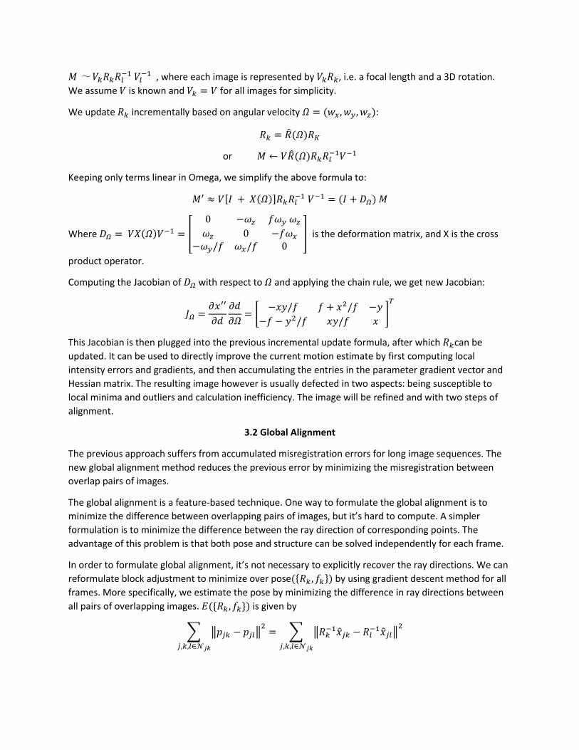
except for a certain degree of luminance difference, as shown in Figure 3 and 4. For Dif-Tough tasks,

where we have big camera angle change or big camera location change in the input image sequence, the

results are still good besides that input images have irregular or imbalanced areas in the result

panoramas as in Figure 5 and 6. This is acceptable because the irregular areas are due to the lack of

information that should not be compensated by the algorithm. For dataset in Dif-Large, the result is not

satisfactory. As in both cases, the output panorama only consists of latter parts of the input image

sequence. This is because the images contain features that are too distant to be fit into one panorama,

either since the image size is too large or that the sequence is long, i.e., there are 5 large-sized images to

be stitched while the fifth image is too distant from the first three. When combining images based on

their extracted features, this leads to the weird rotation angle thus resulting in some portion of the

earlier panorama being behind the latter panorama, resulting in severe loss of information in the final

stitching as in Figure 7 and 8. Another downside of SIFT is that it is of higher time complexity and

consumes slightly more time than SURF but still within a reasonable range.

Figure 3: Easy Task 4 Input

Figure 4: SIFT Output on Easy Task

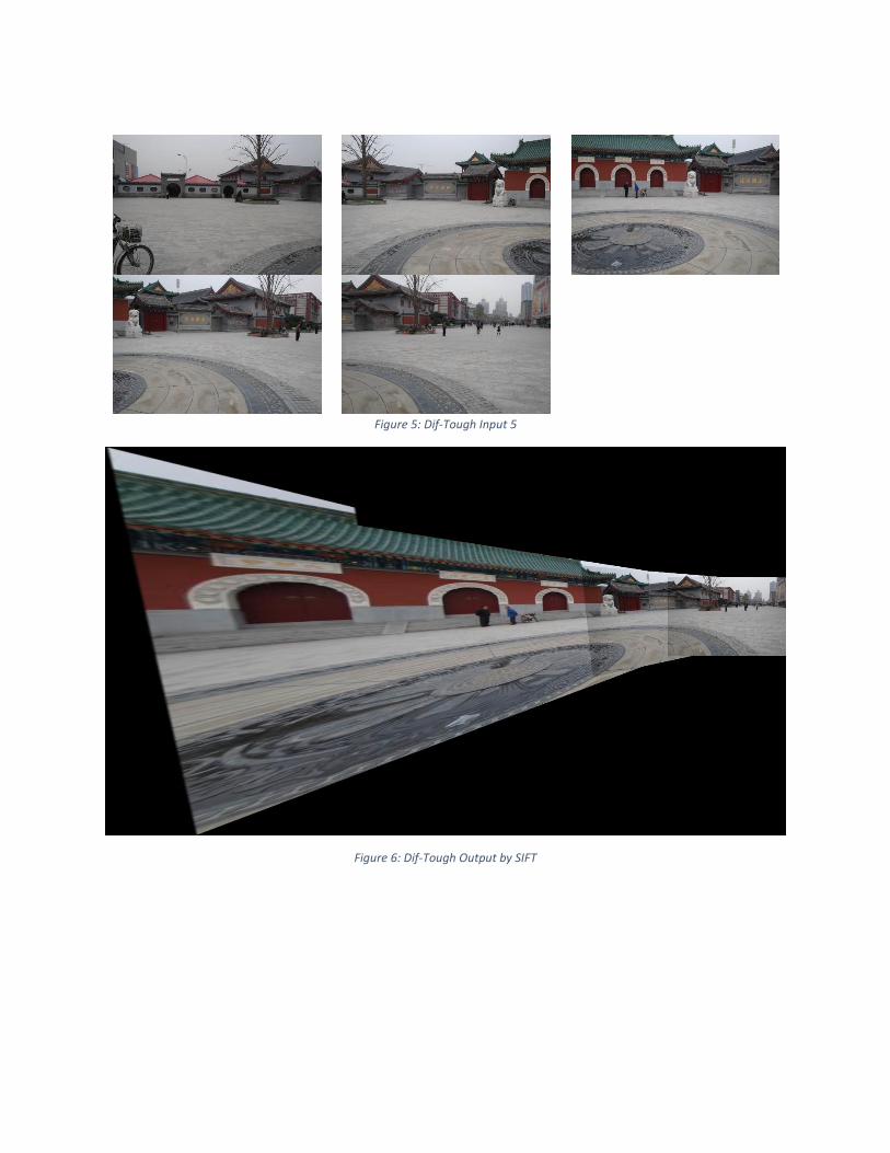
Figure 5: Dif-Tough Input 5

Figure 6: Dif-Tough Output by SIFT

Figure 7: Dif-Large Input

Figure 8: Dif-Large Bad Output with Loss of Information

SURF algorithm, in contrast to SIFT, has overall more stable but a bit worse performance. It is good that

SURF runs a bit faster than SIFT, but it also means that it does not spend that much time and effort into

calculating the features in matching. Also, it requires an additional parameter to work relatively well: the

threshold for hessian keypoint detector. From experiments of [16], We figure out that a value of 500

generally works well. With such value, we get results that are still not as good as SIFT algorithms, which

contain obvious detachment in objects and edges that are not fitting well enough. Different from SIFT,

we are able to form a complete panorama from dataset #3 in Dif-Large, however, most likely because

this algorithm did not apply that strict of an angle to images when stitching. If a real-time photo-purpose

video panorama is the goal, this algorithm is better than SIFT.

There are also aspects that does not concern the quality of panorama. For instance, the algorithms

handle the non-identical overlapping parts differently. Though SURF and SIFT both weigh more on the

latest images, AutoStitch uses average method.

7 Future Works

To further improve the performance of the method, we plan on balancing contrast and brightness

between stitched images on the zones where they touch or overlap. We could try to determine the

histogram equalization function on the zone where images will touch or overlap and apply the

equalization functions that accomplish this on the entire images. Also, we could balance our algorithms

to have higher level of tolerance to errors in camera locations and to have more robust ways to stitch

the images based on their extracted features, in order to give a more natural looking panorama in one

rectangular piece, instead of the current twisted ones.

8 References

[1] Heung-Yeung Shum and Richard Szeliski. Construction and Refinement of Panoramic Mosaics with

Global and Local Alignment. International Conference on Computer Vision, 1998, 48 (2) :953

[2] Tian-Zhu Xiang, Gui-Song Xia, Xiang Bai and Liangpei, Zhang. Image Stitching by Line-guided Local

Warping with Global Similarity Constraint. Pattern Recognition. 83. 10.1016/j.patcog.2018.06.013.

[3] J. Zaragoza, T. Chin, M. S. Brown and D. Suter, "As-Projective-As-Possible Image Stitching with

Moving DLT," 2013 IEEE Conference on Computer Vision and Pattern Recognition, Portland, OR, 2013,

pp. 2339-2346.

[4] C. Lin, S. U. Pankanti, K. N. Ramamurthy and A. Y. Aravkin, "Adaptive as-natural-as-possible image

stitching," 2015 IEEE Conference on Computer Vision and Pattern Recognition (CVPR), Boston, MA, 2015,

pp. 1155-1163.

[5] J. R. Bergen, P. Anandan, K. J. Hanna, R. Hingorani, "Hierarchical model-based motion estimation",

Second European Conference on Computer Vision (ECCV'92), pp. 237-252, 1992-May.

[6] S. E. Chen, "QuickTime VR - an image-based approach to virtual environment navigation", Computer

Graphics (SIGGRAPH'95), pp. 29-38, 1995-August.

[7] S. B. Kang, R Weiss, "Characterization of errors in compositing panoramic images", IEEE Computer

Society Conference on Computer Vision and Pattern Recognition (CVPR'97), pp. 103-109, 1997-June.

[8] R. Kumar, P. Anandan, M. Irani, J. Bergen, K. Hanna, "Representation of scenes from collections of

images", IEEE Workshop on Representations of Visual Scenes, pp. 10-17, 1995-June.

[9] H. S. Sawhney, "Simplifying motion and structure analysis using planar parallax and image warping",

Twelfth International Conference on Pattern Recognition (ICPR'94), vol. A, pp. 403-408, 1994-October.

[10] H.-Y. Shum, R. Szeliski, Panoramic image mosaicing, September 1997.

[11] R. Szeliski, "Video mosaics for virtual environments", IEEE Computer Graphics and Applications, pp.

22-30, March 1996.

[12] R. Szeliski, S. B. Kang, "Direct methods for visual scene reconstruction", IEEE Workshop on

Representations of Visual Scenes, pp. 26-33, 1995-June.

[13] R. Szeliski, H.-Y. Shum, "Creating full view panoramic image mosaics and texture-mapped models",

Computer Graphics (SIGGRAPH'97) Proceedings, pp. 251-258, 1997-August.

[14] David G Lowe, “Distinctive Image Features from Scale-Invariant Keypoints,” International Journal of

Computer Vision, vol.50, No. 2, 2004, pp.91-110.

[15] Bay H., Tuytelaars T., Van Gool L. (2006) SURF: Speeded Up Robust Features. In: Leonardis A.,

Bischof H., Pinz A. (eds) Computer Vision – ECCV 2006. ECCV 2006. Lecture Notes in Computer Science,

vol 3951. Springer, Berlin, Heidelberg

[16] Hussein, Walid & A. Salama, Mostafa & Ibrahim, Osman. (2016). Image Processing Based Signature

Verification Technique to Reduce Fraud in Financial Institutions. MATEC Web of Conferences. 76. 05004.

10.1051/matecconf/20167605004.