® IDEAS Image Data Exploration and Analysis Software User’s Manual Version 2.0 July, 2006 Amnis Corporation 2505 Third Avenue, Suite 210 Seattle, WA 98121 Phone: 206-374-7000 Toll free: 800-730-7147 www.amnis.com i

Welcome message from author
This document is posted to help you gain knowledge. Please leave a comment to let me know what you think about it! Share it to your friends and learn new things together.
Transcript
®IDEAS
Image Data Exploration and Analysis Software User’s Manual
Version 2.0 July, 2006
Amnis Corporation 2505 Third Avenue, Suite 210 Seattle, WA 98121 Phone: 206-374-7000 Toll free: 800-730-7147 www.amnis.com
i

Patents and Trademarks Amnis Corporation's technologies are protected under one or more of the following U.S. Patent Numbers: 6,211,955; 6,249,341; 6,473,176; 6,507,391; 6,532,061; 6,563,583; 6,580,504; 6,583,865; 6,608,680; 6,608,682; 6,618,140; 6,671,044; 6,707,551; 6,763,149; 6,778,263; 6,875,973; 6,906,792; 6,934,408; 6,947,128; 6,947,136; 6,975,400; 7,006,710; 7,009,651. Additional U.S. and corresponding foreign patent applications are pending.
Amnis, the Amnis logo, IDEAS, ImageStream, and INSPIRE are registered or pending U.S. trademarks of Amnis Corporation.
Microsoft, Excel, and Windows are registered trademarks of Microsoft Corporation.
Disclaimers The screen shots presented in this manual were created using the Microsoft® Windows® XP operating system and may vary slightly from those created using other operating systems.
The Amnis® ImageStream® cell analysis system is for research use only and not for use in diagnostic procedures.
Technical Assistance Amnis Corporation 2505 Third Avenue, Suite 210 Seattle, WA 98121 Phone: 206-374-7000 Toll free: 800-730-7147 www.amnis.com
i
Table of Contents
Preface .................................................................................................................5 How to use this manual................................................................................................................ 5
Introducing the IDEAS® Application .....................................................................6 Overview of the IDEAS® Application............................................................................................ 6 Hardware and Software Requirements........................................................................................ 7
Hardware Requirements .......................................................................................................... 7 Software Requirements............................................................................................................ 7
Installing and Upgrading the IDEAS® Application........................................................................ 7 Installing the IDEAS® Application ............................................................................................. 7 Upgrading the IDEAS® Application........................................................................................... 8 Setting Up Your Computer to Run the IDEAS® Application ..................................................... 8 Setting the Screen Resolution.................................................................................................. 8 Viewing File Name Extensions................................................................................................. 8 Copying the Example Data Files.............................................................................................. 9
Understanding the Data Analysis Workflow ........................................................10 Understanding the Data File Types.....................................................................11
Overview of the Data File Types................................................................................................ 11 Raw Image File ...................................................................................................................... 11 Compensated Image File ....................................................................................................... 11 Data Analysis File................................................................................................................... 12 Template................................................................................................................................. 12 Compensation Matrix File....................................................................................................... 12
Viewing and Changing the Application Defaults ........................................................................ 13 Applying Compensation ......................................................................................14
Overview of Compensation........................................................................................................ 14 Creating a New Matrix File......................................................................................................... 14 Applying Compensation to the Control Files.............................................................................. 24 Using MTF Correction................................................................................................................ 25
Managing Files....................................................................................................26 Opening Data Files .................................................................................................................... 26 Merging Raw Image Files .......................................................................................................... 30 Saving Data Files....................................................................................................................... 31
Saving Data Analysis Files..................................................................................................... 31 Saving Compensated Image Files ......................................................................................... 32 Saving Templates................................................................................................................... 32
1
Creating Data Files from Populations ........................................................................................ 33 Exporting Data ........................................................................................................................... 34 Batch Processing ....................................................................................................................... 36
Using the Data Analysis Tools ............................................................................41 Overview of the Data Analysis Tools ......................................................................................... 41 Using the Image Gallery ............................................................................................................ 42
Overview of the Image Gallery ............................................................................................... 43 Setting the Image Gallery Properties ..................................................................................... 45 Working with Individual Images.............................................................................................. 51 Creating Tagged Populations................................................................................................. 51
Using the Analysis Area............................................................................................................. 55 Overview of the Analysis Area ............................................................................................... 55 To manipulate the Analysis Area............................................................................................ 56 Creating Graphs ..................................................................................................................... 56 Creating Regions on Graphs.................................................................................................. 62 Analyzing Images ................................................................................................................... 68 Adding Text to the Analysis Area ........................................................................................... 72
Using the Statistics Area............................................................................................................ 73 Overview of the Statistics Area .............................................................................................. 73 Viewing the Population Statistics ........................................................................................... 73 Viewing the Object Feature Values........................................................................................ 74 Viewing the Compensation Matrix.......................................................................................... 75
Using the Feature Manager ....................................................................................................... 76 Overview of the Feature Manager.......................................................................................... 76 Understanding the Base Features ......................................................................................... 79
Using the Mask Manager ........................................................................................................... 82 Overview of the Mask Manager.............................................................................................. 82 Working with the Mask Manager ............................................................................................ 82
Using the Filter Manager............................................................................................................ 89 Using the Population Manager................................................................................................... 90 Using the Instant Classifier ........................................................................................................ 94
Creating Reports.................................................................................................95 Printing Reports ......................................................................................................................... 95 Exporting Data ........................................................................................................................... 98
Understanding the IDEAS® Features ................................................................101 Overview of the IDEAS® Features ........................................................................................... 102 The Base Features at a Glance............................................................................................... 104 Understanding the Detailed Feature Descriptions................................................................... 111 Understanding the Size Features ............................................................................................ 112
2
The Area Feature ................................................................................................................. 112 The Perimeter Feature ......................................................................................................... 112
Understanding the Location and Shape Features ................................................................... 113 The Aspect Ratio Feature .................................................................................................... 113 The Aspect Ratio Intensity Feature...................................................................................... 113 The Centroid X and Centroid Y Features............................................................................. 114 The Centroid X and Centroid Y Intensity Features .............................................................. 115 Elongatedness...................................................................................................................... 118 The Major Axis Feature ........................................................................................................ 118 The Minor Axis Feature ........................................................................................................ 119 The Major Axis Intensity Feature.......................................................................................... 119 The Minor Axis Intensity Feature.......................................................................................... 120 Negative Curvatures............................................................................................................. 120 The Object Rotation Angle Feature...................................................................................... 120 The Object Rotation Angle Intensity Feature ....................................................................... 120
Understanding the Signal Strength Features........................................................................... 121 The Background Mean Intensity Feature ............................................................................. 121 The Background StdDev Intensity Feature .......................................................................... 121 The Combined Mask Intensity Feature ................................................................................ 121 The Intensity Feature ........................................................................................................... 122 The Mean Intensity Feature ................................................................................................. 122 The Minimum Intensity Feature............................................................................................ 122 The Peak Intensity Feature .................................................................................................. 122 The Total Intensity Feature .................................................................................................. 122
Understanding the Shape and Texture Features..................................................................... 122 The Compactness Feature................................................................................................... 122 The Frequency Feature........................................................................................................ 123 The Gradient Max Feature ................................................................................................... 123 The Gradient RMS Feature .................................................................................................. 123
Understanding the Spot Features............................................................................................ 124 The Spot Count Feature....................................................................................................... 124 The Spot Small Max, Spot Medium Max, Spot Large Max, Spot Small Total, Spot Medium Total, and Spot Large Total Features .................................................................................. 124 The Spot Raw Total and Spot Raw Max Features............................................................... 125
Understanding the Object Information Features...................................................................... 128 The Camera Line Number Feature ...................................................................................... 128 The Camera Timer Feature.................................................................................................. 128 The Flow Speed Feature...................................................................................................... 128 The Object Number Feature................................................................................................. 128
3
Understanding the Comparison Features................................................................................ 128 The Similarity Feature .......................................................................................................... 128 The Normalized Similarity Feature....................................................................................... 128 The Similarity Bright Detail Normalized Feature .................................................................. 129
Glossary............................................................................................................130 Index .................................................................................................................132
4
Preface
How to use this manual The intuitive user interface of the IDEAS application makes it easy for you to explore and analyze data. The application contains powerful algorithms that allow you to create an unlimited number of tailored features for a specific experiment. The application can quantify cellular activity by performing statistical analyses on thousands of events and, at the same time, permit visual confirmation of any individual event. Furthermore, you can operate the application in a batch processing mode and store specific analysis templates for either repeated use or sharing with colleagues.
The fastest way to put the IDEAS application to work is to first skim through this manual—becoming familiar with the application’s structure, compensation, file types, and analysis tools—and then load a sample experiment file to begin exploring the power that the application provides.
This manual provides instruction for using the Amnis IDEAS® application to analyze data files from the Amnis ImageStream cell analysis system. The manual is organized into the following sections:
• Introducing the IDEAS Application—Describes the hardware and software requirements and the installation instructions for running the IDEAS application.
• Understanding the Data Analysis Workflow—Provides a step-by-step description of the workflow for the IDEAS application.
• Understanding the Data File Types--Describes the types of files that the IDEAS application uses and creates.
• Applying Compensation—Describes the procedures that you follow to create a compensation matrix.
• Managing Files —Describes the procedures you follow to open, merge, save, and create new data files.
• Using the Data Analysis Tools—Describes the tools that the IDEAS application makes available for creating masks, features, populations, graphs, and statistics; for performing image analysis; for manipulating the display of imagery; and for reporting results.
• Understanding the IDEAS® Features—Provides an in-depth look at the IDEAS features, including brief mathematical treatments.
5

Introducing the IDEAS® Application
This section supplies an overview of the IDEAS application; the hardware and software requirements for the application; and the procedures for installing, removing, and upgrading the application. The following subsections cover this information:
Overview of the IDEAS® Application
Hardware and Software Requirements
Installing and Upgrading the IDEAS® Application
Overview of the IDEAS® Application The ImageStream cell analysis system possesses unique capabilities that neither flow cytometry nor microscopy alone can deliver. Examples include the analysis of molecule co-localization and translocation, the analysis of cell-to-cell contact regions and signaling interactions, the detection of rare molecules and cells, and a comprehensive classification of large numbers of cells.
To acquire image data from the ImageStream cell analysis system, you use the Amnis INSPIRE™ instrument-control application. To process and analyze the image data, you then make use of the IDEAS application. The latter application contains the algorithms and tools that are needed to preprocess the imagery. These preprocessing algorithms and tools correct for spectral overlap (called compensation) and normalize for systematic instrument biases, including flow variations, spatial alignments, illumination irregularities, and camera pattern noise. After the preprocessing completes, the IDEAS application interrogates the image data, segmenting out cells, nuclei, cytoplasm, FISH spots, beads, and other objects of interest. After the segmentation completes, the application calculates the values for up to 200 standard features per object, to be used in subsequent analyses. Finally, the application displays imagery and feature-calculation results, and it defines cell populations in a host of plots and histograms. Either a default template or a custom assay template that you have selected contains the plots and histograms.
You can further explore the data by using the data analysis tools. For example, you can identify populations of cells by drawing regions on histograms or scatter plots, by tagging individual objects, or by using filters. The IDEAS application provides standard distribution statistics for all defined populations.
The application also contains tools that allow you to view grayscale and pseudocolor images, to apply gains and thresholds, and to build composite images. For individual images, tools are available that allow you to examine pixel intensities, to create line profiles of pixel intensities, and to compute the distribution statistics of the pixels in a region of an image. Both morphological measurements and intensity information are available for calculating feature values and for building classifiers. Histograms and scatter plots display feature data graphically, and the population distribution statistics include a variety of calculations such as the mean, standard deviation, and coefficient of variation (CV).
6

Hardware and Software Requirements This section states the minimum and the recommended hardware and software requirements for running the IDEAS application.
Hardware Requirements The minimum hardware requirements are 512 MB of RAM and a 1-GHz processor. However, due to the large size of the image files that the ImageStream cell analysis system creates, a larger amount of RAM will prevent paging and thus increase performance.
Software Requirements You must have Windows XP, Windows 2000, or a later version of the operating system installed on your computer. The latest service pack and any critical updates for the operating system must be included. You must also install the Microsoft .NET Framework 1.1, which requires Microsoft Internet Explorer 5.01 or later.
Important: If the software requirements are not met, Setup will not block installation nor provide any warnings.
Note that service packs and critical updates are available from the Microsoft Security Web Site.
Installing and Upgrading the IDEAS® Application This section contains the following subsections, which describe how to install and upgrade the IDEAS application:
Installing the IDEAS® Application
Upgrading the IDEAS® Application
Setting Up Your Computer to Run the IDEAS® Application
Installing the IDEAS® Application If the IDEAS application has previously been installed, the previous version must be removed before you can install the new version. See Upgrading the IDEAS® Application.
To install the IDEAS® software 1. Insert the CD or DVD that is labeled IDEAS application, and view the contents in My
Computer or Windows Explorer. 2. Double-click Setup.exe. 3. Follow the instructions until the installation process has completed.
An icon appears on the desktop, and IDEAS Application appears on the All Programs menu.
7
Upgrading the IDEAS® Application To upgrade the IDEAS application, you must remove the existing version before you can install the upgrade.
Upgrading will not affect any data files or templates that you have created. However, upgrading might update the default template.
To upgrade the IDEAS® software 1. On the Start menu, point to Control Panel, and then click Add or Remove Programs. 2. Click IDEAS Application, and then click Remove. 3. When the removal has completed, close the installer. 4. Install the upgrade version. To do so, see Installing the IDEAS® Application.
Setting Up Your Computer to Run the IDEAS® Application Setting the Screen Resolution
Viewing File Name Extensions
Copying the Example Data Files
Setting the Screen Resolution Confirm that the screen resolution is adequate for the IDEAS application. To be able to view the entire application window, you must set the width of the screen resolution to a minimum of 1024 pixels.
To set the screen resolution 1. On the Start menu, point to Control Panel, and then click Display. 2. Click the Settings tab, and then set the screen resolution.
Viewing File Name Extensions When loading a file, the IDEAS application uses the file name extension to determine what the file type is. It will be easier for you to distinguish raw image files, compensated image files, and data analysis files from each other if Windows Explorer does not hide the extensions.
To view file name extensions 1. In Windows Explorer, click Folder Options on the Tools menu. 2. Click the View tab, and make sure that the Hide extensions for known file types check
box is not selected. 3. Click OK.
8

Copying the Example Data Files If the CD or DVD includes data files, copy them to a single directory on your hard drive. Note that the default data directory is installation directory\ImageStreamData, where installation directory is the directory that you installed the IDEAS application in. For example, the default data directory might be C:\Program Files\AmnisCorporation\IDEAS\ImageStreamData.
To copy the example data files 1. Copy the data files. 2. Right-click the directory that contains the data files, and click Properties. 3. Clear the Read-only check box. 4. Click OK.
9

Understanding the Data Analysis Workflow
To analyze data, you begin by creating a fluorescence compensation matrix to remove fluorescence that leaks into nearby channels so that you may accurately depict the correct amount of fluorescence in each cell image. If fluorescence compensation is required, you first need a valid compensation matrix. The compensation matrix is created by using control files that were collected by the INSPIRE application. Once the compensation matrix is made you begin to analyze data files by opening a raw image file (.rif file) that was generated by the INSPIRE application.
Opening the .rif file causes the IDEAS application to perform corrections on the imagery and to apply the selected compensation, resulting in a new compensated image file (.cif file). The application then calculates feature values and shows the data as specified by the selected template. You are then able to save your analysis as a data analysis file (.daf file). This workflow is shown by the following diagram.
1. Create Compensation matrix if necessary 2. Open the .rif file and apply a compensation matrix and template 3. Analyze the experimental data using data analysis tools 4. Save data files, templates and create reports
Experimental
.rif file
.cif file
INSPIRE™
.daf file Save .daf file.
IDEAS®
Save experimental template.
Control
.rif files
Data Collection Data Correction and Compensation Data Analysis
Create compensation matrix file (.ctm file).
Apply experimental or default template.
Open .rif file.
Apply newor existing .ctm file.
Create reports: statistics, graphs, feature data,
and images.
1
2
3
4
10
Understanding the Data File Types
This section contains the following subsections, which describe the files that the IDEAS application creates and uses, the recommended directory organization, and the how to view and change the application defaults:
Overview of the Data File Types
Viewing and Changing the Application Defaults
Overview of the Data File Types Data from the ImageStream cell analysis system is collected and managed using three types of data files: raw image, compensated image, and data analysis. After sample acquisition, the INSPIRE application saves a raw image file (.rif file), which contains instrument setup data and uncorrected image data. The IDEAS application uses the .rif file to create a compensated image file (.cif file), which contains imagery that has been corrected for variations in the camera background, camera gains, flow speed, and vertical and horizontal positioning between channels. When it creates the .cif file, the IDEAS application also performs fluorescence compensation if necessary. The .cif file serves as a database of images that the IDEAS application uses for feature-value calculations and imagery display. Finally, the IDEAS application loads the .cif file into a template to create a data analysis file (.daf file), which is the working data file that contains the calculated feature values, the graphs, and the statistics that are used for analysis.
You can create multiple .cif files from a single .rif file. To do so, simply apply a different fluorescence compensation matrix each time you open the .rif file and choose a unique name for the .cif file. Similarly, you can create multiple .daf files from a single .cif file by applying different analysis templates.
Even though Windows does not treat file names as case sensitive, the IDEAS application depends on the case-sensitive .rif, .cif, and .daf file name extensions to identify the file types.
Raw Image File The INSPIRE application saves the image data that was acquired by the ImageStream cell analysis system to a .rif file. This file contains the pixel intensity data that the camera collected for each object that the instrument detected. The file also contains the instrument settings that were used for data collection.
Compensated Image File The IDEAS application creates a .cif file by segmenting regions of interest in a .rif file. The segmentation algorithm defines the boundaries of each object, creating a mask that is used for calculating feature values. You can request that the IDEAS application perform pixel-by-pixel fluorescence compensation prior to segmentation by applying a compensation matrix.
During the creation of the .cif file, the application makes corrections to the imagery by removing artifacts that are due to variability in the flow speed, camera background, and brightfield gains. Additionally, the application aligns the objects to subpixel accuracy, which allows the viewing of multichannel, composite imagery and the calculation of multichannel feature values, such as the Similarity value.
11
Data Analysis File The IDEAS application creates a .daf file while it is loading a .cif file into a template. The .daf file allows you to visualize and analyze the imagery that the .cif file contains. The .daf file contains feature definitions, population definitions, calculated feature values, image display settings, and definitions for graphs and statistics. Loading a .daf file restores the application to the same state it was in when the file was saved.
Note: When it is opened, the .cif file must be located in the same directory as the .daf file. The reason is that the images used for analysis are stored in the .cif file, not in the .daf file.
Template The IDEAS application saves the set of instructions for an analysis session to a template (.ast file). Note that a template contains no data; it simply contains the structure for the analysis. This structure includes definitions for features, graphs, regions, and populations; image viewing settings; channel names; and statistics settings.
The \templates subdirectory (under the directory where the IDEAS application was installed) contains the default template, named default.ast. Because a template is required for loading a .cif file, you must use the default template to create the first .daf file. After you save a custom template, you can use it for any subsequent loads of .cif files.
Note: The default template may change between releases of the IDEAS application software.
Compensation Matrix File The IDEAS application saves the compensation data that is created and saved during the spectral compensation of control files to a compensation matrix file (.ctm file). This file has no associated object data; it is created and saved to be applied to experimental files.
12

Viewing and Changing the Application Defaults A file is automatically saved to the appropriate default directory. To view or change these defaults, click Application Defaults on the Analysis menu, and the Directories tab will be displayed, as shown in the following figure. To view or change the default color or symbol for populations, click the Populations tab. To view or change the default filter range, click the Filters tab.
13

Applying Compensation
This section contains the following subsections, which describe how to build a compensation matrix and verify that it is correct:
Overview of Compensation
Creating a New Matrix File
Applying Compensation to the Control Files
Using MTF Correction
Overview of Compensation Spectral compensation corrects imagery for fluorescence that leaks into nearby channels so that you may accurately depict the correct amount of fluorescence in each cell image. For example, the light from one fluorochrome may appear primarily in Channel 3, but some of the light from this fluorochrome may appear in Channel 4, as well, because the emission spectrum of the probe extends beyond the Channel 3 spectral bandwidth. The light from a second fluorochrome may appear primarily in Channel 4 but, unless you subtract the light emitted by the first fluorochrome into Channel 4, you cannot generate images that accurately represent the distribution of the second fluorochrome.
The IDEAS application builds a matrix of compensation values by using one or more control file. A control file contains singly stained cells. You can mix singly stained cells and run them together, but you must be careful that the fluorochromes do not bleed onto other singly stained cells. Because it is critical that matrix values be calculated from intensities derived from a sole source of light, control files are collected without brightfield illumination. The IDEAS application performs brightfield compensation when it loads a .rif file.
Creating a New Matrix File The procedure for creating a compensation matrix for an experiment has several steps:
1. Open the compensation window. 2. Load singly stained control files. 3. Identify single cells from the controls. 4. Choose the singly stained populations. 5. Calculate the matrix. 6. Inspect the matrix and refine the populations, if necessary. 7. Optionally, apply the matrix to the control file. 8. Save the matrix.
14

To begin creating a new compensation file 1. Click New Matrix on the Compensation menu. The compensation panel appears in the
lower-left corner of the application window.
To load fluorescence control files 2. Click Add. Navigate to the fluorescence control files. Select the files and then click Open.
Note: The fluorescence control files contain the singly stained controls for each fluorochrome in the experiment, collected with no brightfield illumination. All the control files are in the .rif format.
3. Click Remove to delete a selected file from the list. 4. Click Advanced to open the Advanced Compensation Correction window, which
allows you to turn on MTF correction.
15

5. If you want to apply MTF correction to the controls files, select Perform MTF correction and then click OK. (For more information, see Using MTF Correction.)
Note: A change in the instrument has made the scatter control file obsolete.
6. Click Load Files. If more than one control file exists, they are merged together. You can choose to save this merged file.
7. Click Yes to save the file and to name it. Click No to create the merged file but discard it after the matrix is built. The control files are merged into a single .rif file. The progress is shown in the Creating merged .rif file window.
Background and spatial offset corrections are performed. The progress is shown in the Processing Status window.
16

The IDEAS application creates a .cif file and loads the images. The progress is shown in the Processing Status window.
A dot plot of scatter area (cell size) versus gradient max (focus quality) appears in the Analysis Area.
To create a population to use for compensation 8. Use the plot to select a subpopulation of single cells for subsequent fluorescence
compensation. 9. Remove any doublets because they may be stained with more than one fluorochrome.
From this subpopulation, you can later select singly stained populations and assign them to their appropriate color channels. (For more information, see Creating Regions on Graphs.)
10. If necessary, click the Resize and Zoom buttons on the graph toolbar to more clearly see the population of interest.
11. Using one of the region buttons on the toolbar, draw a region that contains only the cells you want to use for determining compensation. You can click a point on the graph and view the image to help you decide where the region boundaries should be. A new region and population are created.
12. Enter a name in the Create a Region window shown.
17
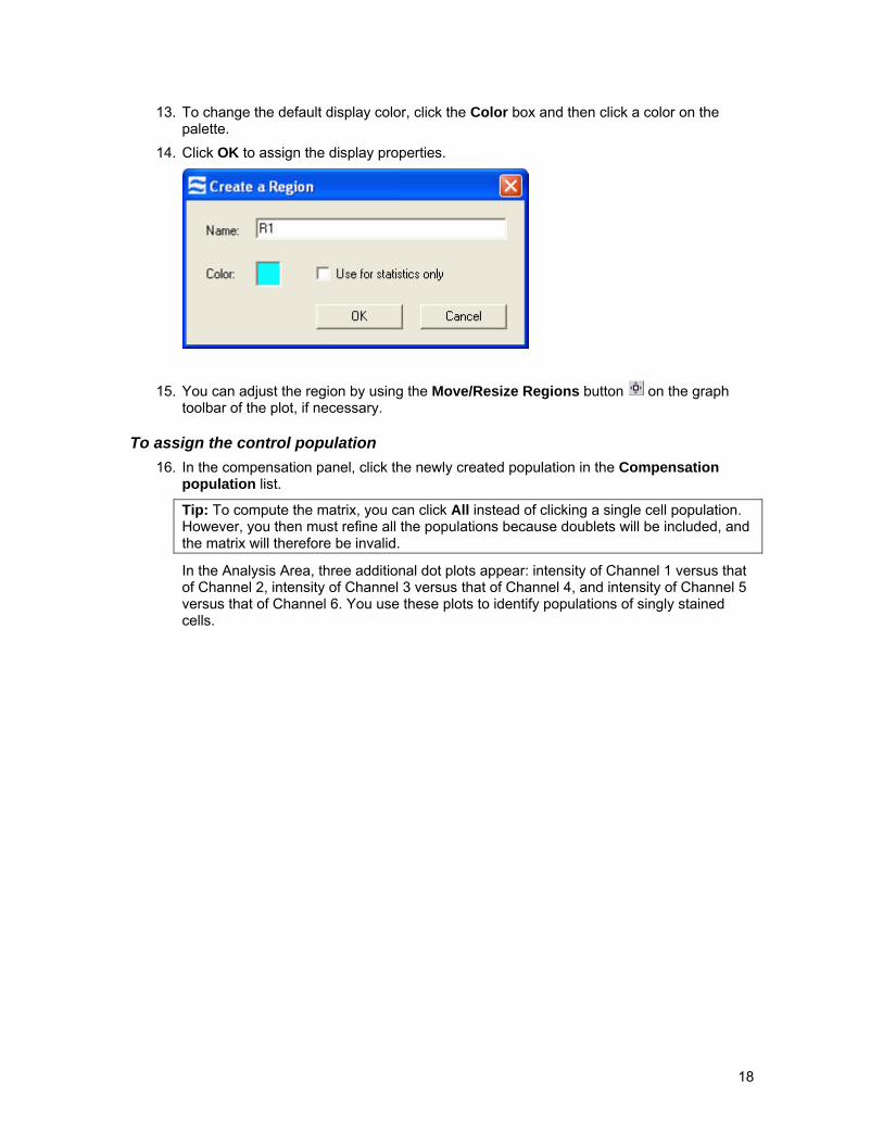
13. To change the default display color, click the Color box and then click a color on the palette.
14. Click OK to assign the display properties.
15. You can adjust the region by using the Move/Resize Regions button on the graph toolbar of the plot, if necessary.
To assign the control population 16. In the compensation panel, click the newly created population in the Compensation
population list.
Tip: To compute the matrix, you can click All instead of clicking a single cell population. However, you then must refine all the populations because doublets will be included, and the matrix will therefore be invalid.
In the Analysis Area, three additional dot plots appear: intensity of Channel 1 versus that of Channel 2, intensity of Channel 3 versus that of Channel 4, and intensity of Channel 5 versus that of Channel 6. You use these plots to identify populations of singly stained cells.
18

Note: The IDEAS application automatically finds the singly stained populations. The automatically generated control populations appear on the graphs. Green corresponds to the Channel 3 positive control population, red to the Channel 5 positive control population, and fuchsia to the Channel 6 positive control population. You can create new scatter plots by using the Analysis Area toolbar. For example, a 4_Intensity versus 5_Intensity plot may be useful.
17. To show the legend, right-click inside the graph and then choose Show/Hide Legend. 18. For each fluorochrome, identify a positive control population and assign it to the proper
channel in the compensation panel. 19. You can use the automatically generated control populations as they are, or you can
refine them and create different populations by using the region tools. For more information, see Creating Regions on Graphs . By default, the populations are named 3_Positive, 5_Positive, and so on. You can view the populations in the Image Gallery. Some populations may be empty.
To assign the positive populations to the channels 20. When you are satisfied with the populations, assign them to the appropriate channels by
using the Positive populations lists. Assign populations only to the channels that correspond to the fluorochromes used in the experiment.
19
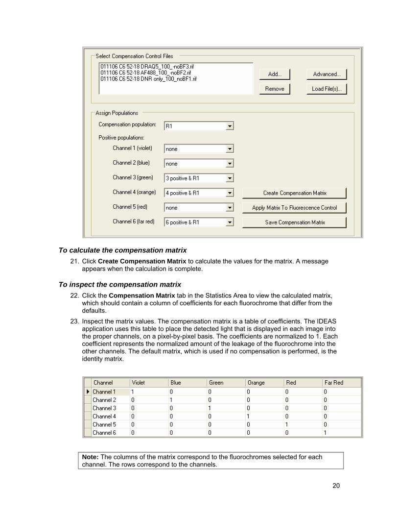
To calculate the compensation matrix 21. Click Create Compensation Matrix to calculate the values for the matrix. A message
appears when the calculation is complete.
To inspect the compensation matrix 22. Click the Compensation Matrix tab in the Statistics Area to view the calculated matrix,
which should contain a column of coefficients for each fluorochrome that differ from the defaults.
23. Inspect the matrix values. The compensation matrix is a table of coefficients. The IDEAS application uses this table to place the detected light that is displayed in each image into the proper channels, on a pixel-by-pixel basis. The coefficients are normalized to 1. Each coefficient represents the normalized amount of the leakage of the fluorochrome into the other channels. The default matrix, which is used if no compensation is performed, is the identity matrix.
Note: The columns of the matrix correspond to the fluorochromes selected for each channel. The rows correspond to the channels.
20

24. Verify that no coefficients are larger than 1. 25. Verify that, in a column corresponding to a fluorochrome, the coefficients decrease from
the assigned channel. In other words, leakage should be greater in the channels nearest to the assigned channel.
26. Verify that the coefficient is larger in the channel to the right of the 1 (below when looking at the table) than to the left of the 1 (above) and decreases in subsequent channels to the right. Remember that fluorescence always extends in the long-wavelength (red-shifted) direction from the exciting light.
27. Verify that there are no changes from the identity matrix in the columns where there are no fluorochromes assigned including the scatter and brightfield channels.
21
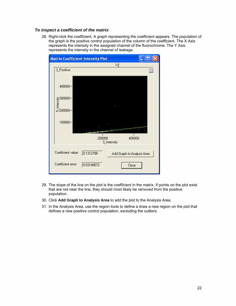
To inspect a coefficient of the matrix 28. Right-click the coefficient. A graph representing the coefficient appears. The population of
the graph is the positive control population of the column of the coefficient. The X Axis represents the intensity in the assigned channel of the fluorochrome. The Y Axis represents the intensity in the channel of leakage.
29. The slope of the line on the plot is the coefficient in the matrix. If points on the plot exist that are not near the line, they should most likely be removed from the positive population.
30. Click Add Graph to Analysis Area to add the plot to the Analysis Area. 31. In the Analysis Area, use the region tools to define a draw a new region on the plot that
defines a new positive control population, excluding the outliers.
22
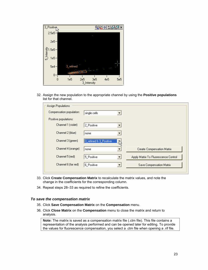
32. Assign the new population to the appropriate channel by using the Positive populations list for that channel.
33. Click Create Compensation Matrix to recalculate the matrix values, and note the
change in the coefficients for the corresponding column. 34. Repeat steps 28–33 as required to refine the coefficients.
To save the compensation matrix 35. Click Save Compensation Matrix on the Compensation menu. 36. Click Close Matrix on the Compensation menu to close the matrix and return to
analysis.
Note: The matrix is saved as a compensation matrix file (.ctm file). This file contains a representation of the analysis performed and can be opened later for editing. To provide the values for fluorescence compensation, you select a .ctm file when opening a .rif file.
23
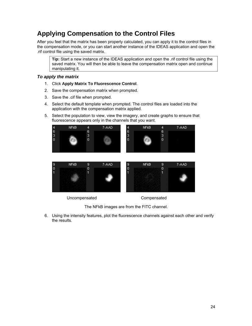
Applying Compensation to the Control Files After you feel that the matrix has been properly calculated, you can apply it to the control files in the compensation mode, or you can start another instance of the IDEAS application and open the .rif control file using the saved matrix.
Tip: Start a new instance of the IDEAS application and open the .rif control file using the saved matrix. You will then be able to leave the compensation matrix open and continue manipulating it.
To apply the matrix 1. Click Apply Matrix To Fluorescence Control. 2. Save the compensation matrix when prompted. 3. Save the .cif file when prompted. 4. Select the default template when prompted. The control files are loaded into the
application with the compensation matrix applied. 5. Select the population to view, view the imagery, and create graphs to ensure that
fluorescence appears only in the channels that you want.
Uncompensated Compensated
The NFkB images are from the FITC channel.
6. Using the intensity features, plot the fluorescence channels against each other and verify the results.
24
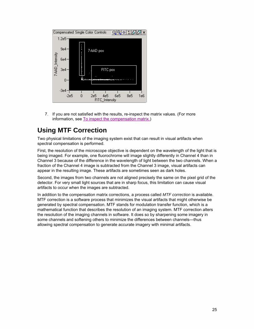
7. If you are not satisfied with the results, re-inspect the matrix values. (For more information, see To inspect the compensation matrix.)
Using MTF Correction Two physical limitations of the imaging system exist that can result in visual artifacts when spectral compensation is performed.
First, the resolution of the microscope objective is dependent on the wavelength of the light that is being imaged. For example, one fluorochrome will image slightly differently in Channel 4 than in Channel 3 because of the difference in the wavelength of light between the two channels. When a fraction of the Channel 4 image is subtracted from the Channel 3 image, visual artifacts can appear in the resulting image. These artifacts are sometimes seen as dark holes.
Second, the images from two channels are not aligned precisely the same on the pixel grid of the detector. For very small light sources that are in sharp focus, this limitation can cause visual artifacts to occur when the images are subtracted.
In addition to the compensation matrix corrections, a process called MTF correction is available. MTF correction is a software process that minimizes the visual artifacts that might otherwise be generated by spectral compensation. MTF stands for modulation transfer function, which is a mathematical function that describes the resolution of an imaging system. MTF correction alters the resolution of the imaging channels in software. It does so by sharpening some imagery in some channels and softening others to minimize the differences between channels—thus allowing spectral compensation to generate accurate imagery with minimal artifacts.
25

Managing Files
This section contains the following subsections, which describe how to open, merge, save, and create data files:
Opening Data Files
Merging Raw Image Files
Saving Data Files
Creating Data Files from Populations
Exporting Data
Batch Processing
Opening Data Files Use the File menu, which is shown in the following figure, to open, save, and close image and analysis files and to quit the IDEAS application. (If you are opening a .rif file for the first time and do not have a compensation matrix, read the Applying Compensation section before proceeding.)
You can open any of three file types: .rif, .cif, or .daf.
When you open a .rif file, the IDEAS application corrects each image for the spatial alignment between channels, camera background normalization, flow speed, and brightfield gain normalization. If you want fluorescence compensation, you must provide the matrix at this time. In nearly all cases, you will want to correct for spectral overlap. The application performs the corrections by using calibration information that was saved to the .rif file during acquisition. To correct for spectral overlap, you must create a compensation matrix by using the control files that were collected for a particular experiment. (For more information, see Applying Compensation.)
Applying these corrections to the .rif file generates a .cif file that the IDEAS application uses to display images and calculate feature values.
When you open a .cif file, you must select a template, which provides the initial characteristics of the analysis. Opening the .cif file causes the IDEAS application to calculate feature values and to use populations, graphs, and image viewing settings to display the cells as defined by the template.
Immediately after opening a .cif file, you should save the analysis as a .daf file. Doing so saves the calculated feature values so that they will not need to be recalculated.
To open a .daf file, the IDEAS application requires the .cif file to reside in the same directory. The .daf file does not contain any image data, so you can think of the .cif file as the database that
26
contains the imagery. Because all the feature values have been saved in it, the .daf file should open quickly. Note that opening a .daf file restores the state of the IDEAS application to the same analysis state that existed when the .daf file was created.
Note: If the .daf file is large, it may take some time to calculate the statistics for graphs.
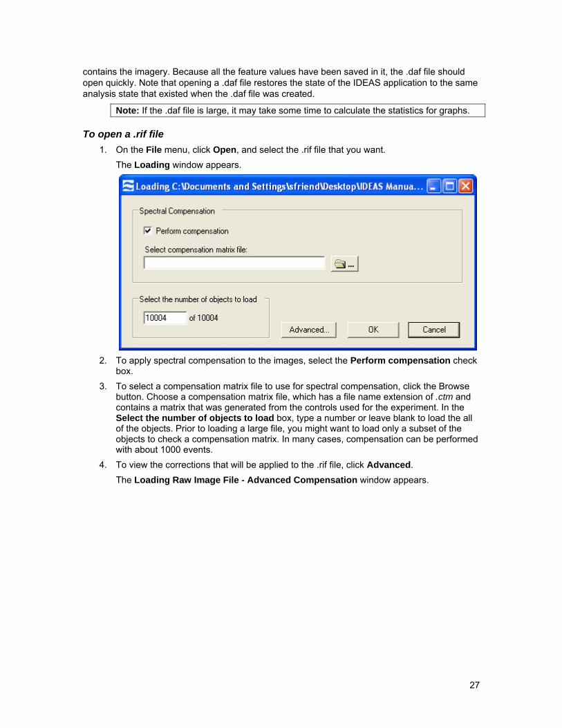
To open a .rif file 1. On the File menu, click Open, and select the .rif file that you want.
The Loading window appears.
2. To apply spectral compensation to the images, select the Perform compensation check
box. 3. To select a compensation matrix file to use for spectral compensation, click the Browse
button. Choose a compensation matrix file, which has a file name extension of .ctm and contains a matrix that was generated from the controls used for the experiment. In the Select the number of objects to load box, type a number or leave blank to load the all of the objects. Prior to loading a large file, you might want to load only a subset of the objects to check a compensation matrix. In many cases, compensation can be performed with about 1000 events.
4. To view the corrections that will be applied to the .rif file, click Advanced. The Loading Raw Image File - Advanced Compensation window appears.
27

5. Make any changes to the corrections that you need, and then click OK. Most often, the
defaults will be adequate. For some older data files, you may need to provide control files for the spatial alignment and camera background. To use values from other .rif files, click Change Alignment Offsets and/or Change Correction Offsets. You can also turn on modulation transfer function (MTF) correction. (For more information, see Using MTF Correction.)
6. Click OK. The Save As Compensated Image (.cif) File dialog box appears.
7. Name the .cif file that will be created. The Select Template File dialog box appears.
8. Select and open a template (.ast file) that will define the initial analysis state.
Note: The IDEAS application provides a default template. However, you will find it useful to create and save your own templates for specific experimental procedures.
The IDEAS application processes and loads the .rif file the progress is shown by a progress bar. The application then creates the .cif file.
To open a .cif file 1. On the File menu, click Open, and select the .cif file that you want.
28

2. Select a template (.ast file) to define the initial analysis state. Note that the IDEAS application provides a default template. However, it is useful to create and save your own templates for specific experimental procedures.
3. Click Open. During the opening of a .cif file, the IDEAS application calculates the values of the features that are defined in the template you selected. The progress is shown by a progress bar. After the application has successfully opened the .cif file, you should save the analysis as a .daf file.
To open a .daf file
• On the File menu, click Open, and select the .daf file that you want. The progress is shown by a progress bar. The state of the IDEAS application is restored to what it was when the .daf file was saved.
To open multiple .cif files, combine their data, and create a single .daf file 1. On the File menu, click Open Multiple Files.
The Load Multiple .cif Files window appears.
2. Click Add Files, and select the .cif files that you want. The file names appear in the Files to Load list.
3. For each file, type the number of objects to load. For each file, the IDEAS application creates a population and displays a default population name.
4. If you want, change any or all of the default population names. 5. Type or select the resulting .cif file name.
29

If you type or select an existing file name, a warning appears that asks you to verify the overwriting of the file.
6. Browse to select a template. 7. If you want, change the resulting .daf file name.
If you type or select an existing file name, a warning appears that asks you to verify the overwriting of the file.
8. Click OK. The IDEAS application loads the .cif files and creates a single .cif and .daf file.
Merging Raw Image Files You can merge .rif files together for analysis.
To merge .rif files 1. On the Tools menu, click Merge .rif Files.
The Merge Raw Image Files window appears.
2. To select the .rif files to merge, click Add Files.
The .rif file names appear in the list. 3. If you want to remove a file from the list, select it and then click Remove Files. 4. When the merge list is complete, click OK.
The Save Merged Raw Image (.rif) File dialog box appears. 5. Type a unique file name. 6. Click Save.
The Creating merged .rif file window appears. When the merge is complete, the Merged .rif Created message appears.
30
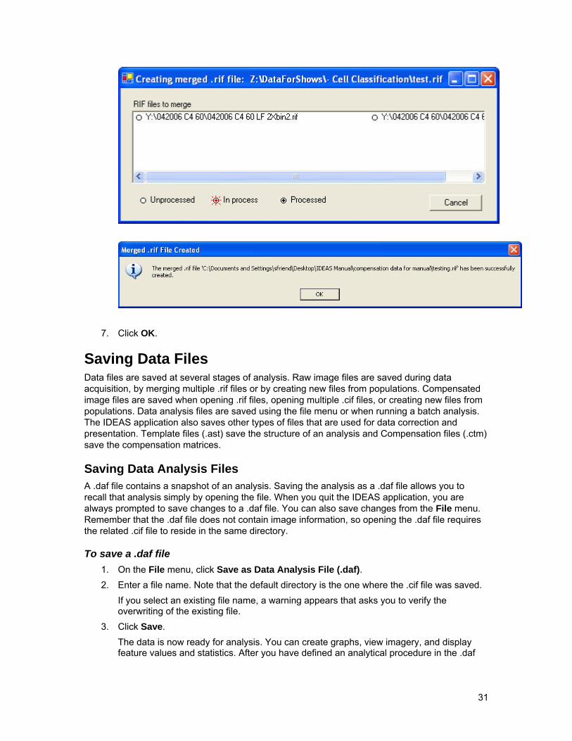
7. Click OK.
Saving Data Files Data files are saved at several stages of analysis. Raw image files are saved during data acquisition, by merging multiple .rif files or by creating new files from populations. Compensated image files are saved when opening .rif files, opening multiple .cif files, or creating new files from populations. Data analysis files are saved using the file menu or when running a batch analysis. The IDEAS application also saves other types of files that are used for data correction and presentation. Template files (.ast) save the structure of an analysis and Compensation files (.ctm) save the compensation matrices.
Saving Data Analysis Files A .daf file contains a snapshot of an analysis. Saving the analysis as a .daf file allows you to recall that analysis simply by opening the file. When you quit the IDEAS application, you are always prompted to save changes to a .daf file. You can also save changes from the File menu. Remember that the .daf file does not contain image information, so opening the .daf file requires the related .cif file to reside in the same directory.
To save a .daf file 1. On the File menu, click Save as Data Analysis File (.daf). 2. Enter a file name. Note that the default directory is the one where the .cif file was saved.
If you select an existing file name, a warning appears that asks you to verify the overwriting of the existing file.
3. Click Save. The data is now ready for analysis. You can create graphs, view imagery, and display feature values and statistics. After you have defined an analytical procedure in the .daf
31
file, you can save the file as a template, which allows you to use the procedure for analyzing other files.
Saving Compensated Image Files The IDEAS application creates and saves a .cif file when a .rif file is opened. By default, the application names the .cif file with the same name that the .rif file has, replacing the .rif extension with .cif. The application also places the .cif file in the same directory as the .rif file. The .cif file will be larger than the .rif file because the .cif file contains masking information as well as corrected and/or compensated images.
Saving Templates Saving an analysis as a template allows you to apply the structure of the analysis to other .cif files. A template includes all graph definitions, Image Gallery settings, feature definitions, and statistics settings. No data is saved in a template. Therefore, selected images and populations that are dependent on specific objects, such as tagged populations, are not saved.
To save a template 1. On the File menu, click Save As Template File (.ast).
A Save File dialog box appears. 2. Enter the name of the file to save. 3. Click Save.
If you select an existing file name, a warning appears that asks you to verify the overwriting of the existing file.
Tip: You can change the default template directory by clicking Application Defaults on the Analysis menu.
32
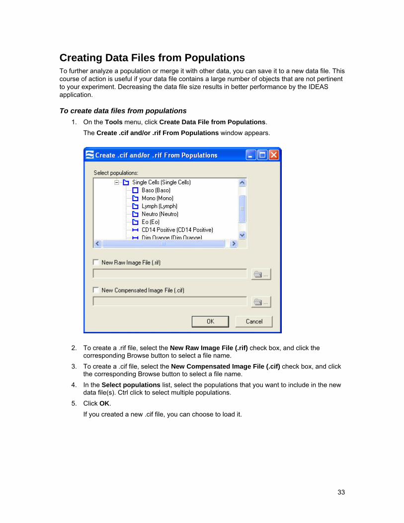
Creating Data Files from Populations To further analyze a population or merge it with other data, you can save it to a new data file. This course of action is useful if your data file contains a large number of objects that are not pertinent to your experiment. Decreasing the data file size results in better performance by the IDEAS application.
To create data files from populations 1. On the Tools menu, click Create Data File from Populations.
The Create .cif and/or .rif From Populations window appears.
2. To create a .rif file, select the New Raw Image File (.rif) check box, and click the corresponding Browse button to select a file name.
3. To create a .cif file, select the New Compensated Image File (.cif) check box, and click the corresponding Browse button to select a file name.
4. In the Select populations list, select the populations that you want to include in the new data file(s). Ctrl click to select multiple populations.
5. Click OK. If you created a new .cif file, you can choose to load it.
33
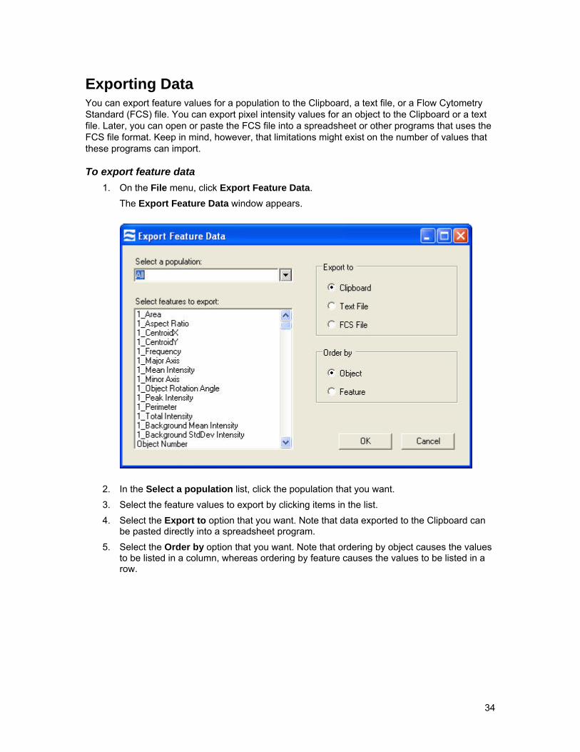
Exporting Data You can export feature values for a population to the Clipboard, a text file, or a Flow Cytometry Standard (FCS) file. You can export pixel intensity values for an object to the Clipboard or a text file. Later, you can open or paste the FCS file into a spreadsheet or other programs that uses the FCS file format. Keep in mind, however, that limitations might exist on the number of values that these programs can import.
To export feature data 1. On the File menu, click Export Feature Data.
The Export Feature Data window appears.
2. In the Select a population list, click the population that you want. 3. Select the feature values to export by clicking items in the list. 4. Select the Export to option that you want. Note that data exported to the Clipboard can
be pasted directly into a spreadsheet program. 5. Select the Order by option that you want. Note that ordering by object causes the values
to be listed in a column, whereas ordering by feature causes the values to be listed in a row.
34

To export pixel data 1. On the File menu, click Export Image Pixel Values.
The Export Image Pixel Values window appears.
2. Select the object to export. 3. Select Clipboard or File. 4. Click OK.
35
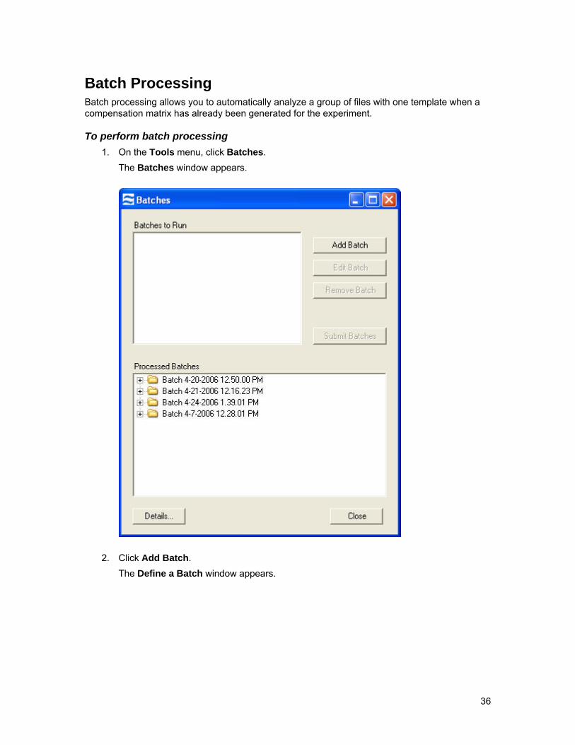
Batch Processing Batch processing allows you to automatically analyze a group of files with one template when a compensation matrix has already been generated for the experiment.
To perform batch processing 1. On the Tools menu, click Batches.
The Batches window appears.
2. Click Add Batch. The Define a Batch window appears.
36
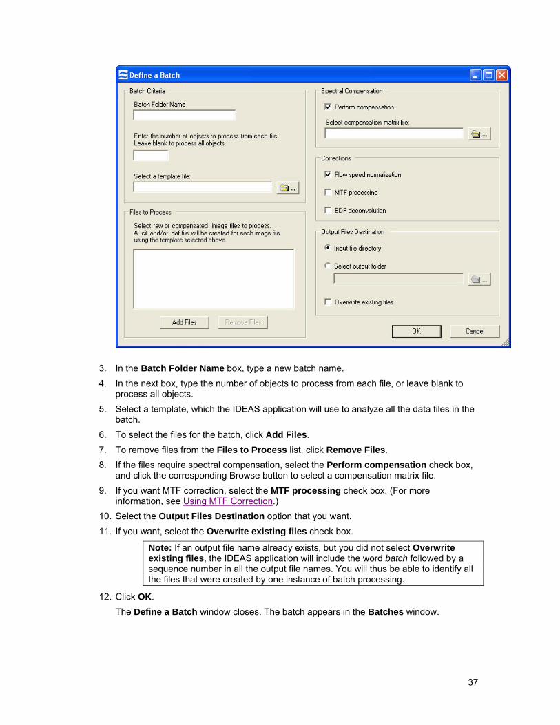
3. In the Batch Folder Name box, type a new batch name. 4. In the next box, type the number of objects to process from each file, or leave blank to
process all objects. 5. Select a template, which the IDEAS application will use to analyze all the data files in the
batch. 6. To select the files for the batch, click Add Files. 7. To remove files from the Files to Process list, click Remove Files. 8. If the files require spectral compensation, select the Perform compensation check box,
and click the corresponding Browse button to select a compensation matrix file. 9. If you want MTF correction, select the MTF processing check box. (For more
information, see Using MTF Correction.) 10. Select the Output Files Destination option that you want. 11. If you want, select the Overwrite existing files check box.
Note: If an output file name already exists, but you did not select Overwrite existing files, the IDEAS application will include the word batch followed by a sequence number in all the output file names. You will thus be able to identify all the files that were created by one instance of batch processing.
12. Click OK. The Define a Batch window closes. The batch appears in the Batches window.
37

13. If you want to remove a batch from the Batches to Run list, click it and then click Remove Batch.
14. If you want to edit a batch in the Batches to Run list, click it and then click Edit Batch. The Define a Batch window reappears.
15. When you are satisfied with the Batches to Run list, click the batch that you want to process and then click Submit Batches. The progress is displayed in the Processing Batch window.
Tip: To cancel the batch processing at any time, click Cancel. The IDEAS application will complete the file it is working on.
When the batch processing is complete, the IDEAS application saves the .rif, .cif, and .daf files in the batch results directory. In the Batches window, a list of processed batches appears in the Processed Batches list. If a batch did not successfully complete, it will appear in red.
Tip: To display the error that occurred during processing, right-click the batch.
38

16. If you want a batch report, double-click the batch in the Processed Batches list of the Batches window.
39
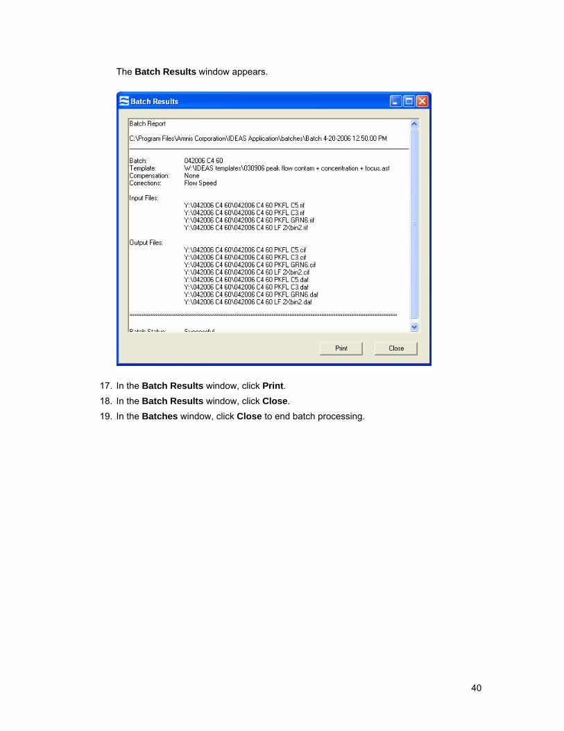
The Batch Results window appears.
17. In the Batch Results window, click Print. 18. In the Batch Results window, click Close. 19. In the Batches window, click Close to end batch processing.
40
Using the Data Analysis Tools
This section contains the following subsections, which describe how to view imagery; graph data; create populations by drawing regions in graphs, by filtering, or by tagging objects; perform statistical analysis of data; and create new features:
Overview of the Data Analysis Tools
Using the Image Gallery
Using the Analysis Area
Using the Statistics Area
Using the Feature Manager
Using the Mask Manager
Using the Filter Manager
Using the Population Manager
Using the Instant Classifier
Overview of the Data Analysis Tools The IDEAS application provides a powerful tool set that allows you to explore and analyze data. The rich feature set lets you create hundreds of your own features to differentiate objects and statistically quantify your results.
As shown in the following figure, the application window is divided into three panels—Image Gallery, Statistics Area, and Analysis Area—which each provide the corresponding tools that you can use for data analysis.
41

Statistics Area
Image Gallery
Analysis Area
You can create populations of objects by tagging hand-selected images, drawing regions on graphs, and using Boolean logic to combine existing populations. Another way to create a population of objects is by basing it on the similarity of a set of feature values to one or more cells in the data set. After you have created a population, you can view it in the Image Gallery or plot it on a graph. You can view the statistics for a population in the Statistics Area.
Graphs show data plotted with one or two feature values, and tools are provided that allow you to draw regions for the purpose of generating new populations. You can show any population on a plot.
Selecting an individual data point in a graph allows you to view it in the Image Gallery or look at its feature values in the Statistics Area. Any object that is selected in the Image Gallery is also shown on the plots in the Analysis Area.
Using the Image Gallery This section contains the following subsections, which describe how to view populations of objects in various ways, view masks, customize the Image Gallery display, and hand-select objects for a population:
Overview of the Image Gallery
Setting the Image Gallery Properties
Working with Individual Images
Creating Tagged Populations
42
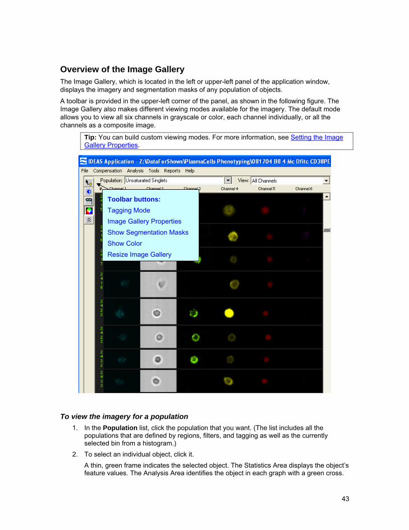
Overview of the Image Gallery The Image Gallery, which is located in the left or upper-left panel of the application window, displays the imagery and segmentation masks of any population of objects.
A toolbar is provided in the upper-left corner of the panel, as shown in the following figure. The Image Gallery also makes different viewing modes available for the imagery. The default mode allows you to view all six channels in grayscale or color, each channel individually, or all the channels as a composite image.
Tip: You can build custom viewing modes. For more information, see Setting the Image Gallery Properties.
Toolbar buttons: Tagging Mode Image Gallery Properties Show Segmentation Masks Show Color Resize Image Gallery
To view the imagery for a population 1. In the Population list, click the population that you want. (The list includes all the
populations that are defined by regions, filters, and tagging as well as the currently selected bin from a histogram.)
2. To select an individual object, click it. A thin, green frame indicates the selected object. The Statistics Area displays the object’s feature values. The Analysis Area identifies the object in each graph with a green cross.
43
Tip: Conversely, clicking a graphical point causes the Image Gallery to highlight and display the corresponding object.
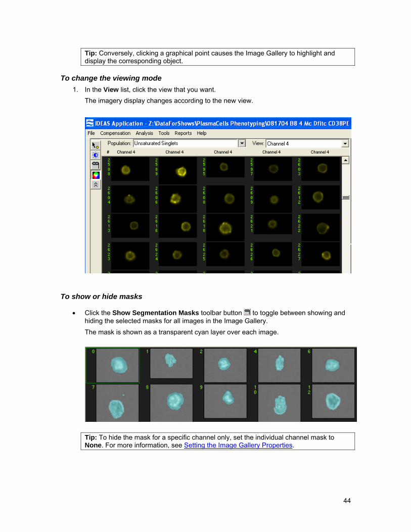
To change the viewing mode 1. In the View list, click the view that you want.
The imagery display changes according to the new view.
To show or hide masks
• Click the Show Segmentation Masks toolbar button to toggle between showing and hiding the selected masks for all images in the Image Gallery.
The mask is shown as a transparent cyan layer over each image.
Tip: To hide the mask for a specific channel only, set the individual channel mask to None. For more information, see Setting the Image Gallery Properties.
44

To show or hide color
• Click the Show Color toolbar button to toggle between showing and hiding the colors for all images in the Image Gallery.
To resize the Image Gallery 1. Click the Resize Image Gallery toolbar button to expand the Image Gallery to the full
height of the application window.
The icon on the toolbar button changes and the Analysis Area shrinks to cover only the lower-right corner of the window.
2. Click the Resize Image Gallery toolbar button again to restore the Image Gallery to its original size.
Setting the Image Gallery Properties When a new data file opens in the default template, you might find it difficult to clearly see cell morphology because the Image Gallery display properties have not yet been properly adjusted for the data set.
Clicking the Image Gallery Properties toolbar button opens the Image Gallery Channel Display Properties window, which contains the following tabs:
• Channels—Allows you to define the name, color, mask, and image display intensity for each channel.
• Views—Allows you to customize the views for the Image Gallery.
• Composites—Allows you to adjust the amount of color from a channel that is included in a composite image.
To customize the Image Gallery display properties 1. Click the Image Gallery Properties toolbar button to begin.
The Image Gallery Channel Display Properties window appears with the Channels tab displayed.
45
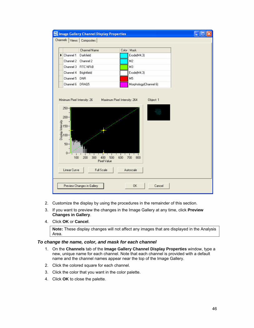
2. Customize the display by using the procedures in the remainder of this section. 3. If you want to preview the changes in the Image Gallery at any time, click Preview
Changes in Gallery. 4. Click OK or Cancel.
Note: These display changes will not affect any images that are displayed in the Analysis Area.
To change the name, color, and mask for each channel 1. On the Channels tab of the Image Gallery Channel Display Properties window, type a
new, unique name for each channel. Note that each channel is provided with a default name and the channel names appear near the top of the Image Gallery.
2. Click the colored square for each channel. 3. Click the color that you want in the color palette. 4. Click OK to close the palette.
46
Tip: The grayscale image in each channel is assigned a default color for image display in the gallery. Setting the color to white is equivalent to using the original grayscale image. The colors are also used to build composite images.
5. On the mask box for each channel select a mask. See Mask Manager for details on how to create new masks.
To fine-tune the image display intensity for a channel 1. On the Channels tab of the Image Gallery Channel Display Properties window, select
a channel by clicking the gray box to the left of the channel name. The currently selected image is shown in the window and updates as the changes are made.
Note: You will adjust the Display Intensity settings on the graph, which maps the pixel value of an image to the pixel value of the display. The range of display intensities is 0–255; the range of intensities from the camera is 0–1023. The limits of the graph enable you to use the full dynamic range of the display to map the pixel intensities of the image.
At each intensity on the X Axis of the graph, the gray histogram shows the number of pixels in the image. This histogram provides you with a general sense of the range of pixel intensities in the image. The dotted green line maps the pixel intensities to the display intensities, which are in the 0–255 range.
The vertical green line on the left side allows you to set the display pixel intensity to 0 for all intensities that appear to the left of that line. Doing so removes background noise from the image.
The vertical green line on the right side allows you to set the display pixel intensity to 255 for all intensities that appear to the right of that line.
2. Select the object to use for setting the mapping.
Tip: You might need to select different objects for different channels because an object might not fluoresce in all channels.
3. To adjust the pixel mapping for display, drag the vertical green lines by clicking near them (but not near the yellow cross).
Tip: For fluorescence channels, set the vertical green line that appears on the left side to the dimmest pixel in the image and set the right vertical green line to the brightest pixel. To get a good mapping range, adjust the same line so that the yellow cross is centered among the pixel intensities on the X Axis. For the brightfield channel, set the vertical lines to about 50 counts to the right and left of the histogram to produce an image with crisp brightfield contrast.
a. To change the mapping curve to be logarithmic or exponential, drag the yellow cross. b. To restore the mapping to a linear curve, click Linear Curve. c. To set the scale of the X Axis to be 0–1023, click Full Scale. d. To set the scale of the X Axis to the range of the vertical green lines or of all the pixel
intensities for the selected object—whichever is larger—click Autoscale. 4. If you want to preview the changes in the Image Gallery, click Preview Changes in
Gallery. 5. Continue customizing the Image Gallery display properties with another procedure in this
section, or click OK or Cancel to finish.
47
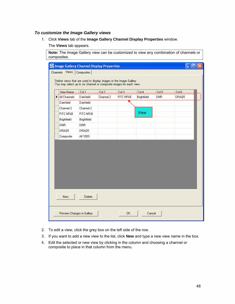
To customize the Image Gallery views 1. Click Views tab of the Image Gallery Channel Display Properties window.
The Views tab appears.
Note: The Image Gallery view can be customized to view any combination of channels or composites.
View
2. To edit a view, click the grey box on the left side of the row. 3. If you want to add a new view to the list, click New and type a new view name in the box. 4. Edit the selected or new view by clicking in the column and choosing a channel or
composite to place in that column from the menu.
48

Note: A blank column cannot precede a defined column. The All Channels view cannot be edited.
5. If you want to delete a view, click the row to select it, and then click Delete. 6. If you want to preview the changes in the Image Gallery, select the view in the Image
Gallery and then click Preview Changes in Gallery. 7. Continue customizing the Image Gallery display properties with another procedure in this
section, or click OK or Cancel to finish.
49

To customize a composite 1. Click the Composites tab in the Image Gallery Channel Display Properties window.
The Composites tab appears.
2. To define a new composite, click New, and then edit the name in the Composite name
box. Otherwise, select the composite you want to customize by clicking it in the Composites list. The selected image appears in the Object box.
3. Change the Channel Color Percentages, which specify the percentage of each channel to include in the composite.
Tip: As you make the changes, the image in the Object box updates accordingly. Setting the amount to zero eliminates the channel from the composite image. The Image Gallery displays the composite image of the selected object and updates the image as changes are made
4. If you want to preview the changes in the Image Gallery, select the view in the Image Gallery and then click Preview Changes in Gallery.
50
5. Continue customizing the Image Gallery display properties with another procedure in this section, or click OK or Cancel to finish.
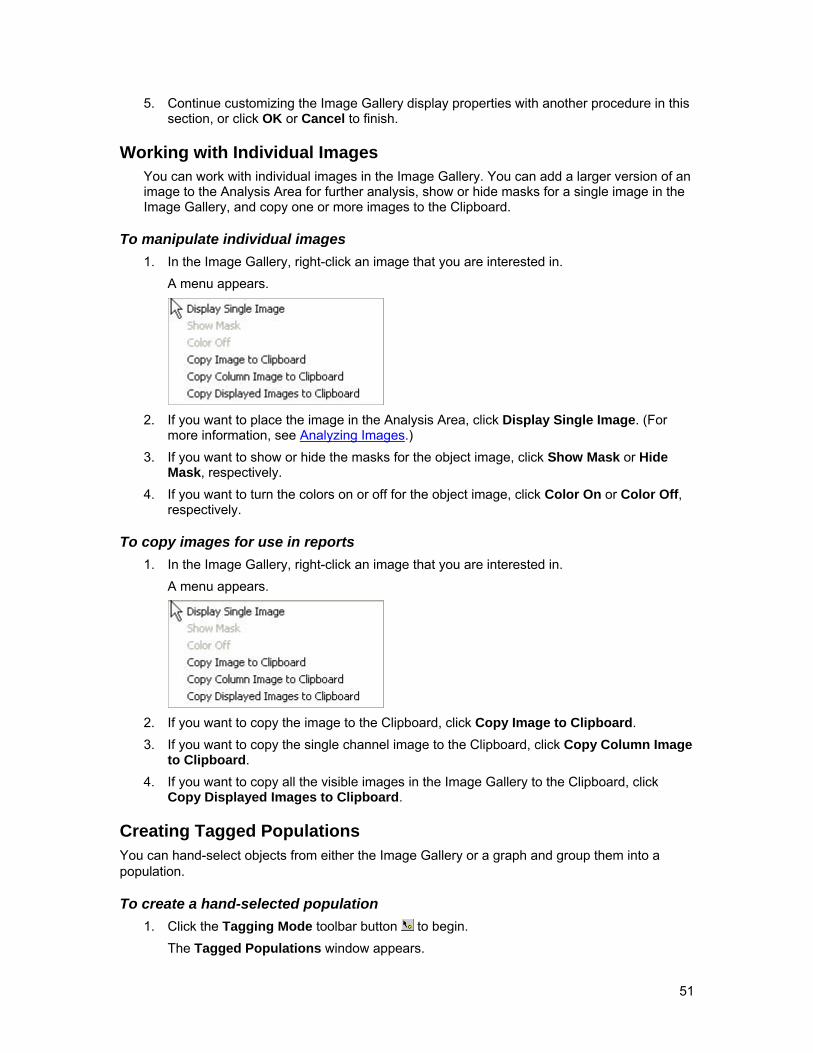
Working with Individual Images You can work with individual images in the Image Gallery. You can add a larger version of an image to the Analysis Area for further analysis, show or hide masks for a single image in the Image Gallery, and copy one or more images to the Clipboard.
To manipulate individual images 1. In the Image Gallery, right-click an image that you are interested in.
A menu appears.
2. If you want to place the image in the Analysis Area, click Display Single Image. (For
more information, see Analyzing Images.) 3. If you want to show or hide the masks for the object image, click Show Mask or Hide
Mask, respectively. 4. If you want to turn the colors on or off for the object image, click Color On or Color Off,
respectively.
To copy images for use in reports 1. In the Image Gallery, right-click an image that you are interested in.
A menu appears.
2. If you want to copy the image to the Clipboard, click Copy Image to Clipboard. 3. If you want to copy the single channel image to the Clipboard, click Copy Column Image
to Clipboard. 4. If you want to copy all the visible images in the Image Gallery to the Clipboard, click
Copy Displayed Images to Clipboard.
Creating Tagged Populations You can hand-select objects from either the Image Gallery or a graph and group them into a population.
To create a hand-selected population 1. Click the Tagging Mode toolbar button to begin.
The Tagged Populations window appears.
51

2. Select Update existing or Create New. 3. If you selected Update existing, click the population to update in the list. 4. In the Image viewing mode list, click the mode that you want. 5. To add or remove an image from the tagged population, double-click either the image in
the Image Gallery or a dot in a bivariate plot.
52

The selected channel image for each tagged cell is displayed in the viewing area of the Tagged Populations window. In the Image Gallery, a small smiley-face icon appears on the left side of each tagged image. Each tagged object is also displayed as a yellow star in a graph.
53
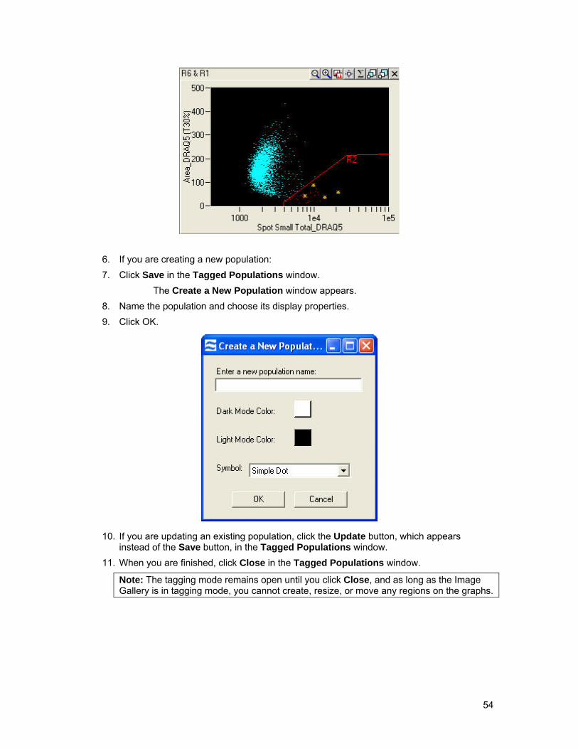
6. If you are creating a new population: 7. Click Save in the Tagged Populations window.
The Create a New Population window appears. 8. Name the population and choose its display properties. 9. Click OK.
10. If you are updating an existing population, click the Update button, which appears instead of the Save button, in the Tagged Populations window.
11. When you are finished, click Close in the Tagged Populations window.
Note: The tagging mode remains open until you click Close, and as long as the Image Gallery is in tagging mode, you cannot create, resize, or move any regions on the graphs.
54

Using the Analysis Area This section contains the following subsections, which describe how to create graphs, analyze images, and use text panels in the Analysis Area of the IDEAS application:
Overview of the Analysis Area
Creating Graphs
Creating Regions on Graphs
Analyzing Images
Adding Text to the Analysis Area
Overview of the Analysis Area The Analysis Area provides display space for individual images, plots of cellular feature values, visualizations of population distributions and statistics, and text annotations. When you expand the Image Gallery, the Analysis Area shrinks to cover only the lower-right corner of the application window. Otherwise, the Analysis Area spans the entire lower portion of the window.
A toolbar is visible on the left side of the Analysis Area. As you can see in the following figure, the toolbar provides tools for creating tagged populations, new regions, and graphs.
Pointer
Tagging Mode
New Histogram
New Scatter Plot
New Text Panel
Line Region
Rectangle Region
Oval Region
Polygon Region
The Pointer tool provides the normal mode of interaction with the graphs. Using the Pointer tool to click a point on a scatter-plot graph causes the IDEAS application to display the corresponding image in the Image Gallery (if the population that is currently displayed in the Image Gallery contains that point). Using the Pointer tool in this manner also causes the application to display the corresponding statistics in the Statistics Area. Clicking the top of a bin in a histogram selects
55

the bin. In the Image Gallery, you can view images of cells in the bin by clicking the Selected Bin population. Clicking the Pointer tool while drawing a region on a graph also cancels the creation of a region.
The Tagging Mode tool allows you to create a population of hand-picked objects. For more information, see Creating Tagged Populations.
As illustrated by the following figure, the Analysis Area can contain seven types of panels: histogram, histogram overlay, scatter plot, channel image, composite image, and text. Each panel will contain its own toolbar and context menu.
Text
Scatter Plots Histogram
Histogram Overlay
Statistics
Composite Image
Channel Images
To manipulate the Analysis Area The analysis area is divided into panels of a fixed size. The size of the panels is automatically adjusted to fit in the available display space. A vertical scroll bar appears when the number of panels exceeds the space available on the window.
1. To expand or contract the analysis area, click the double arrowhead symbol in the Image Gallery.
2. To move a panel, click and drag the upper-left corner and release it in the desired position. The panel will tile to the position that it covers.
3. To delete a panel, click the Delete panel toolbar button in the upper right corner of the panel.
Creating Graphs You can add two types of graphs to the Analysis Area:
• Histogram—Graphs a single feature.
• Scatter Plot—Graphs two features.
56
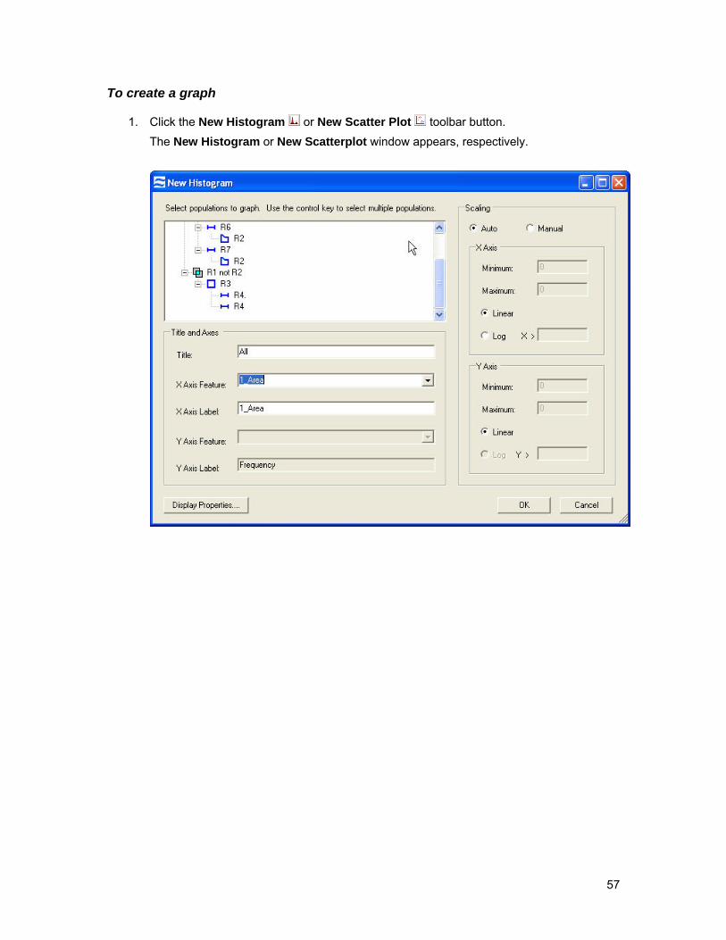
To create a graph
1. Click the New Histogram or New Scatter Plot toolbar button. The New Histogram or New Scatterplot window appears, respectively.
57

2. Select the one or more populations to graph by clicking them. To select more than one population, use the CTRL key.
3. The title defaults to the selected population. You can edit the title. 4. In the X Axis Feature list, click the feature that you want to graph on the X Axis. 5. If you want to change the label for the X axis, edit the text in the X Axis Label box. The
label defaults to the name of the selected feature. 6. If you are creating a scatter plot, select a feature and a label for the Y Axis. 7. Set the scaling for each axis of the graph. (The default is Auto, which allows the
application to automatically scale the graph.) 8. To set minimum and maximum values for an axis, select Manual. 9. Select Linear or Log and enter maximum and minimum limits. 10. If you selected Log, enter the X > value.
58

Note: You can scale the X Axis of a graph or the Y Axis of a scatter plot in one of two modes: Linear or Log. The Linear mode is the default.
The Log mode allows you to logarithmically scale a section of the graph or scatter plot. Selecting this mode causes the IDEAS application to perform bi-exponential plotting. The > X value defines the linear portion of the graph as −X through X. The application plots the values outside of these limits on a logarithmic scale. You can plot negative values as well as positive ones on a logarithmic scale by adjusting the limits.
Take care not to split a population such that it appears to be two separate populations. This splitting is especially likely when negative values exist due to compensation or corrections on the imagery. The graph on the left side was plotted on a linear scale; the ones in the center and on the right side were plotted on logarithmic scales. The graph on the right side split the population because the change from a linear to a logarithmic scale occurred in the middle of the population. The IDEAS application automatically chose 1000 for the scale of the graph that is in the center.
11. To modify the display characteristics of each population or to change the layering order, click Display Properties. The Display Properties window opens.
59

12. Arrange the layering of the populations to allow them to be displayed. 13. If you want, click the button to open the Population Manager. (For more information, see
Population Manager.) 14. If you are creating a histogram, you can customize it by performing the following steps:
a. To fill or not fill the line for a population, select or clear the box. b. If you want, change the bin count. (The default is determined by the X Axis scale of
the plots.) c. Decide whether to plot the Y Axis as a frequency or a normalized frequency
percentage. 15. Click OK twice.
Tip: After you have created a graph, you can change its properties by clicking Graph Properties on the graph context menu. The same window that you used to create the graph will reappear, and you can then make any changes that you want.
60
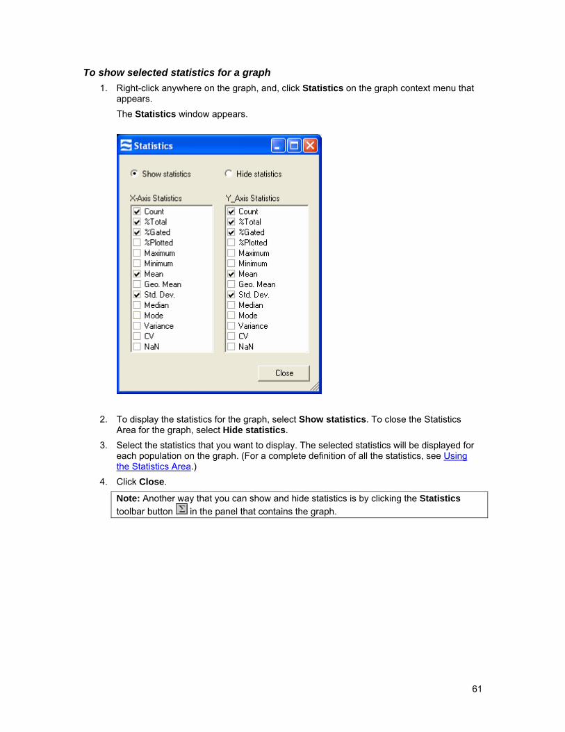
To show selected statistics for a graph 1. Right-click anywhere on the graph, and, click Statistics on the graph context menu that
appears. The Statistics window appears.
2. To display the statistics for the graph, select Show statistics. To close the Statistics Area for the graph, select Hide statistics.
3. Select the statistics that you want to display. The selected statistics will be displayed for each population on the graph. (For a complete definition of all the statistics, see Using the Statistics Area.)
4. Click Close.
Note: Another way that you can show and hide statistics is by clicking the Statistics toolbar button in the panel that contains the graph.
61

To show the legend for a graph 1. Right-click anywhere on the graph, and click Show/Hide Legend on the graph context
menu that appears. If the legend was hidden, it appears on the graph. If the legend was shown, it disappears from the display.
Note: The legend contains an entry for each population on the graph. If the graph is a scatter plot, the legend shows the population and its associated point style and color. If the graph is a histogram or overlay histogram, the legend shows the population name, associated color, and line type.
2. To resize the legend (to see all the populations on the graph), right-click and drag the border. (You cannot resize the legend past the boundary of the graph panel.)
3. To move the legend, click and drag it. (You cannot drag the legend past the boundary of the graph panel, although you can drag it over the statistics if they are displayed.)
Creating Regions on Graphs Regions may be drawn on graphs to create new populations, based on the physical location of objects on a graph, and to compute statistics. Tools for drawing regions are found on the Analysis Area toolbar. A line region may be drawn only on a histogram. All other types of regions may be drawn only on a scatter plot. A region can be copied to another graph. Regions may also be copied from one instance of the IDEAS application to another.
When you draw a region on a histogram or scatter plot, you create a population of objects defined by the region that may be viewed in the Image Gallery or on other graphs. Drawing a region on an overlay histogram does not create a population but simply provides statistics for the graph. A region drawn on an overlay histogram is called a marker.
To draw a line region, oval region, or rectangle region on a graph 1. Click the Line Region , Oval Region , or Rectangle Region button on the
Analysis Area toolbar. 2. Click the graph at the point where you would like to start the region, and drag to the
region endpoint. The region grows as you drag.
62

3. Click again to complete the region. If you are drawing a region on a histogram or scatter plot, the Create a Region window appears.
4. Name the region. 5. Select Use for statistics only if you do not want to create a population from this region. 6. Click OK.
The region appears on the graph with the name and color that you selected.
To draw a polygon region on a graph 1. Click the Polygon Region button on the Analysis Area toolbar. 2. Click the scatter plot at the point where you would like to start the polygon. 3. Click once for each vertex of the polygon.
63
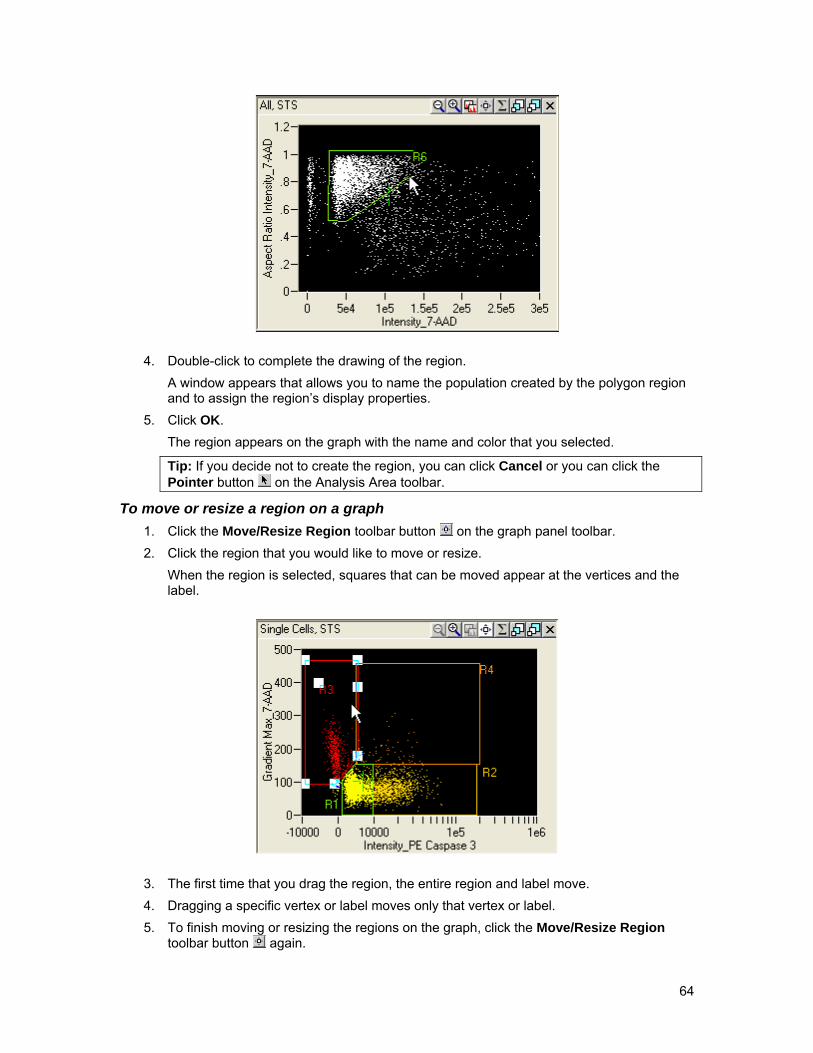
4. Double-click to complete the drawing of the region. A window appears that allows you to name the population created by the polygon region and to assign the region’s display properties.
5. Click OK. The region appears on the graph with the name and color that you selected.
Tip: If you decide not to create the region, you can click Cancel or you can click the Pointer button on the Analysis Area toolbar.
To move or resize a region on a graph
1. Click the Move/Resize Region toolbar button on the graph panel toolbar. 2. Click the region that you would like to move or resize.
When the region is selected, squares that can be moved appear at the vertices and the label.
3. The first time that you drag the region, the entire region and label move. 4. Dragging a specific vertex or label moves only that vertex or label. 5. To finish moving or resizing the regions on the graph, click the Move/Resize Region
toolbar button again.
64
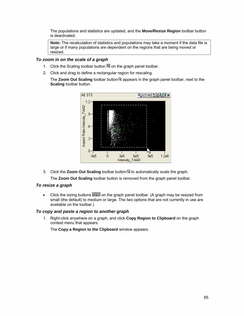
The populations and statistics are updated, and the Move/Resize Region toolbar button is deactivated.
Note: The recalculation of statistics and populations may take a moment if the data file is large or if many populations are dependent on the regions that are being moved or resized.
To zoom in on the scale of a graph 1. Click the Scaling toolbar button on the graph panel toolbar. 2. Click and drag to define a rectangular region for rescaling.
The Zoom Out Scaling toolbar button appears in the graph panel toolbar, next to the Scaling toolbar button.
3. Click the Zoom Out Scaling toolbar button to automatically scale the graph. The Zoom Out Scaling toolbar button is removed from the graph panel toolbar.
To resize a graph
• Click the sizing buttons on the graph panel toolbar. (A graph may be resized from small (the default) to medium or large. The two options that are not currently in use are available on the toolbar.)
To copy and paste a region to another graph 1. Right-click anywhere on a graph, and click Copy Region to Clipboard on the graph
context menu that appears. The Copy a Region to the Clipboard window appears.
65
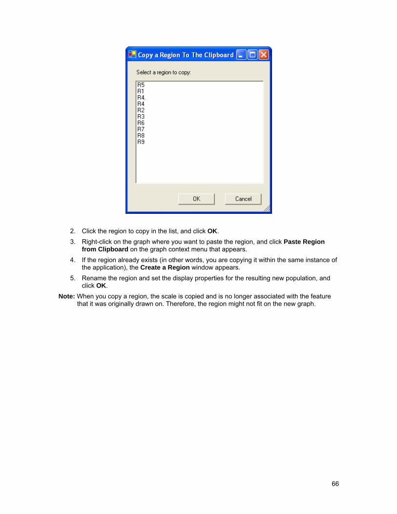
2. Click the region to copy in the list, and click OK. 3. Right-click on the graph where you want to paste the region, and click Paste Region
from Clipboard on the graph context menu that appears. 4. If the region already exists (in other words, you are copying it within the same instance of
the application), the Create a Region window appears. 5. Rename the region and set the display properties for the resulting new population, and
click OK. Note: When you copy a region, the scale is copied and is no longer associated with the feature
that it was originally drawn on. Therefore, the region might not fit on the new graph.
66
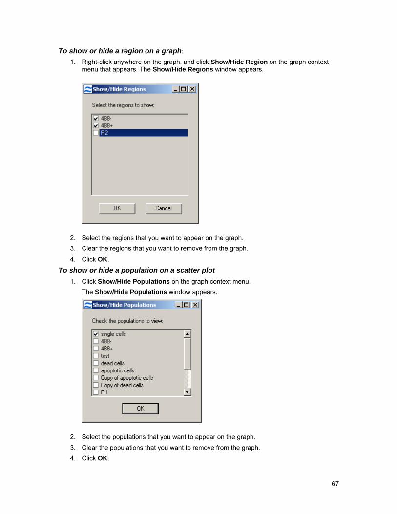
To show or hide a region on a graph: 1. Right-click anywhere on the graph, and click Show/Hide Region on the graph context
menu that appears. The Show/Hide Regions window appears.
2. Select the regions that you want to appear on the graph. 3. Clear the regions that you want to remove from the graph. 4. Click OK.
To show or hide a population on a scatter plot 1. Click Show/Hide Populations on the graph context menu.
The Show/Hide Populations window appears.
2. Select the populations that you want to appear on the graph. 3. Clear the populations that you want to remove from the graph. 4. Click OK.
67
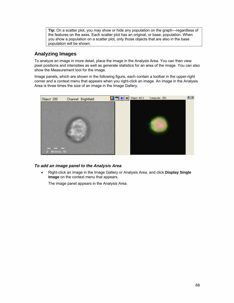
Tip: On a scatter plot, you may show or hide any population on the graph—regardless of the features on the axes. Each scatter plot has an original, or base, population. When you show a population on a scatter plot, only those objects that are also in the base population will be shown.
Analyzing Images To analyze an image in more detail, place the image in the Analysis Area. You can then view pixel positions and intensities as well as generate statistics for an area of the image. You can also show the Measurement tool for the image.
Image panels, which are shown in the following figure, each contain a toolbar in the upper-right corner and a context menu that appears when you right-click an image. An image in the Analysis Area is three times the size of an image in the Image Gallery.
To add an image panel to the Analysis Area • Right-click an image in the Image Gallery or Analysis Area, and click Display Single
Image on the context menu that appears.
The image panel appears in the Analysis Area.
68

To view the individual pixel intensities of a single channel image
• Move the mouse pointer across the image. The pixel positions and intensities appear under the image. (The pixel (0, 0) is positioned at the upper left of the image.)
To display the Measurement tool in an image panel • Right-click the image panel, and click Show Measurement Tool on the context menu
that appears. The 10-micron bar appears.
To examine a line profile or the statistics for an area of an image
• Click and drag to create a boxed area on the image. The Image Statistics window appears next to the image panel. The statistics are calculated for the area that is defined by the box. The line profile (the wavy line in the image panel) represents the pixel intensity at each position along the red line of the box.
69

To change the display properties of an image 1. Click the Channel Display Properties button on the image panel Toolbar.
The Display Properties window appears. 2. For single channel or composite images, click the Image Display tab to adjust the display
intensities of the image. (For more information, see Setting the Image Gallery Properties.) 3. For a composite image, click the Composite tab to adjust the composite color percentage
for each channel of the composite.
70

4. For single channel or composite images, click the Image Display tab to adjust the display intensities of the image.
5. Click OK.
To show or hide the mask for a single channel image
• Click the Mask button on the image panel toolbar, or right-click the image and then click Show/Hide Mask on the image context menu. The mask appears as a transparent cyan overlay on the image.
To turn the color on or off
• Click the Color button on the image panel toolbar, or right-Click the image and then click Color Off or Color On.
71
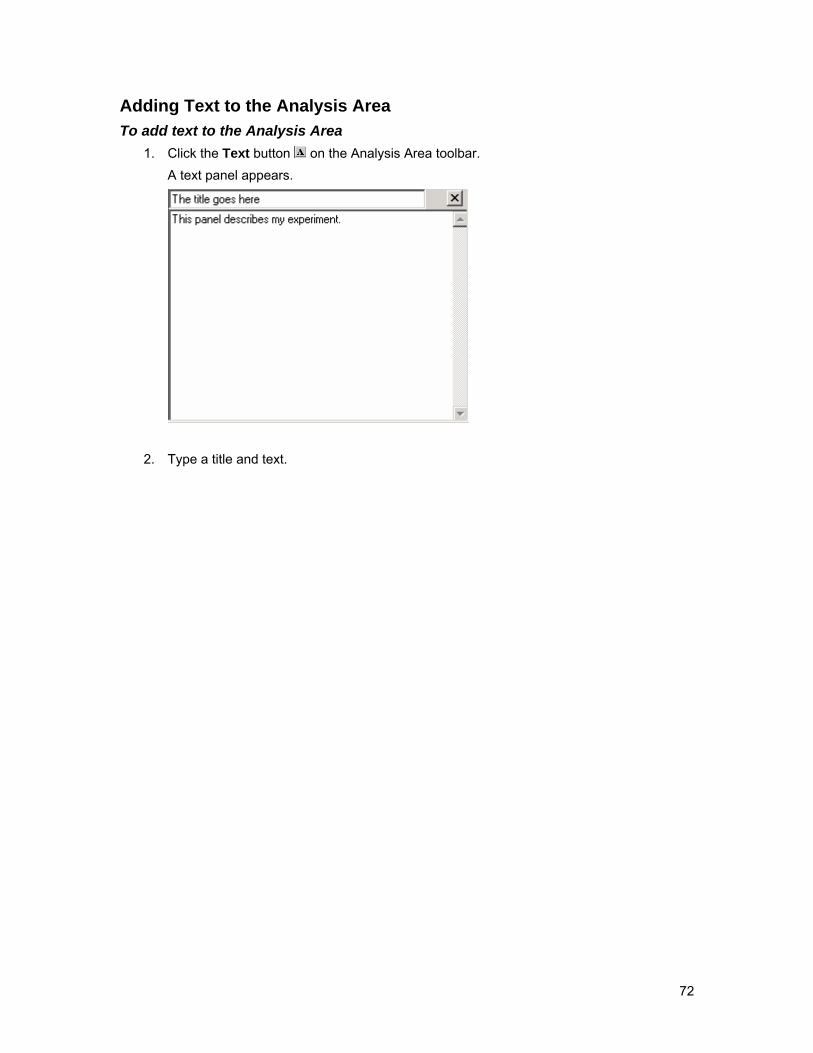
Adding Text to the Analysis Area To add text to the Analysis Area
1. Click the Text button on the Analysis Area toolbar. A text panel appears.
2. Type a title and text.
72
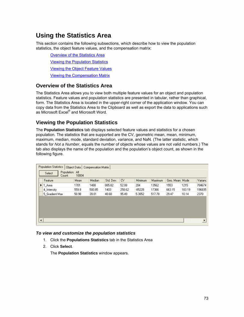
Using the Statistics Area This section contains the following subsections, which describe how to view the population statistics, the object feature values, and the compensation matrix:
Overview of the Statistics Area
Viewing the Population Statistics
Viewing the Object Feature Values
Viewing the Compensation Matrix
Overview of the Statistics Area The Statistics Area allows you to view both multiple feature values for an object and population statistics. Feature values and population statistics are presented in tabular, rather than graphical, form. The Statistics Area is located in the upper-right corner of the application window. You can copy data from the Statistics Area to the Clipboard as well as export the data to applications such as Microsoft Excel® and Microsoft Word.
Viewing the Population Statistics The Population Statistics tab displays selected feature values and statistics for a chosen population. The statistics that are supported are the CV, geometric mean, mean, minimum, maximum, median, mode, standard deviation, variance, and NaN. (The latter statistic, which stands for Not a Number, equals the number of objects whose values are not valid numbers.) The tab also displays the name of the population and the population’s object count, as shown in the following figure.
To view and customize the population statistics 1. Click the Populations Statistics tab in the Statistics Area 2. Click Select.
The Population Statistics window appears.
73

3. Click a population in the Population list. 4. In the Population statistics area, select the statistics that you want to view. 5. In the Features area, select the features that you want to view. 6. Click OK.
The statistics are calculated and shown on the Population Statistics tab.
Viewing the Object Feature Values The Object Data tab, which is shown in the following figure, displays a selected set of feature values for a single object. For each feature, the name, value, and description are shown.
To view and customize the features shown on the Object Data tab 1. Click the Object Data tab in the Statistics Area. 2. Click Select.
The Select Object Features window appears.
74

3. Select the features to view. 4. Click OK.
The features appear on the Object Data tab.
Viewing the Compensation Matrix The Compensation Matrix tab displays the values that are used to perform spectral compensation, as illustrated by the following figure. For more information, see Applying Compensation.
To view the compensation matrix • Click the Compensation Matrix tab in the Statistics Area.
To export or copy statistics
• Right-click the statistics or features shown, and then click Copy data to clipboard. For more information, see Exporting Data.
75

Using the Feature Manager This section describes how to create and delete features, and it provides a high-level description of the base features that are provided by the IDEAS application. The following subsections cover this information:
Overview of the Feature Manager
Understanding the Base Features
Overview of the Feature Manager The IDEAS application defines a set of base features that you can use to create features for each object. To do so, you use the object’s mask or its channel images. After a feature has been created and its value calculated for a population of cells, you can plot the feature values or view them as statistics. For descriptions of all the base features, see Understanding the Base Features.
When the IDEAS application opens a .cif or .rif file, the application calculates the values of features as defined by the selected template. You can refine your template so that it includes only those features of interest for your experiment.
You use the Feature Manager to examine existing features and to define new ones. To gain access to the Feature Manager, click Features on the Analysis menu or on one of the context menus that are available in the histogram and scatter plot panels. While the Feature Manager is open, all calculations for creating graphs and statistics are disabled. However, you may view images and change the population and channel views. When you close the Feature Manager, any changes to feature names, definitions, and values are reflected in any currently displayed graphs and statistics. The values of newly created features are also calculated at this time.
You can create single features and combined features. You create a single feature by selecting a base feature, such as Area or Total Intensity, along with a mask and/or a channel. You create a combined feature by defining a mathematical expression that includes one or more single features.
Some features, such as Area, depend on the boundary of a cell. These features require you to select a mask that defines the portion of the image to use for the calculation. Other features, such as Peak Intensity, depend on pixel intensity measurements and require you to select a channel. Still other features require you to select a mask and one or more channels.
You can add and remove features from the feature list. The feature definitions are stored in templates, so the definitions are available when you analyze multiple data files. The default template includes most of the base features for each channel and channel mask that the feature list contains. Certain features, such as Similarity and Spot, require extensive calculations so the default template does not include them. The reason is to save time when you load files. However, you can add these features to the feature list.
To view existing features 1. Click Features on the Analysis menu or on a graph panel context menu.
The Feature Manager window appears. 2. Click the Single Features tab to view all the single features.
76

3. Click the Combined Features tab to view all the combined features. 4. Click a feature in the Features list to view its definition.
To create a new single feature 1. Click the Single Features tab. 2. Click New.
The Name box and Base Feature list are enabled. 3. Click your choice in the Base Feature list. (If you click ALL FEATURES, the IDEAS
application uses the selected mask and channel to calculates feature values for the entire list of base features. The application automatically names these features with their defaults.) The Mask and Channel lists become visible as required by the feature that you selected.
4. Click the mask and/or channel that you want.
77

5. Enter a unique feature name or click Set Default Name. (The default name is the name of the base feature followed by the text, _channel_mask.)
6. Click Add To List to add the new feature. 7. Click Close.
Note: When you close the Feature Manager, the IDEAS application calculates values for the new features. These calculations may take several minutes, depending on the number and complexity of the new features and the size of the image file.
To create a new combined feature 1. Click the Combined Features tab. 2. Click New.
The editing interface appears.
3. Enter the feature name in the Name box. 4. Use the toolbar to build a mathematical expression of features and operators:
a. To add a feature to the definition, double-click the feature in the Features list, select the feature, and click the leftmost down-arrow button on the toolbar. Alternatively, you can select the feature and then click Add Feature.
b. To add an operator or a parenthesis to the definition, click the corresponding button on the toolbar.
c. To add a number to the definition, enter the number in the box and then click the corresponding down-arrow button.
d. To add a function to the definition, click it in the list and then click the corresponding down-arrow button. The available functions are ABS (absolute), COS (cosine), SIN (sine), SQR (square), and SQRT (square root).
e. To remove an item from the end of the definition, click the left-arrow button on the toolbar.
5. Click Add To List to create the feature.
78

To delete a feature 1. Select one or more features in the Features list by clicking them. To select more than one
feature, use the CTRL key. 2. Click Delete.
Note: Deleting a feature also deletes any populations that are dependent on that feature. Your feature list may become large and unwieldy. You can narrow down the list without deletions by using the Filter button that appears in the Filter Manager. For more information, see Using the Filter Manager.
Understanding the Base Features The base features that the IDEAS application provides are categorized in this section by what they measure: size, location and shape, signal strength, shape and texture, object information, and comparisons. These categories have some overlap. You can apply each feature to any channel and/or mask by using the Feature Manager. For detailed definitions and mathematical formulas, see Understanding the IDEAS® Features.
Size Size measurements are in pixels. Pixel measurements can be converted to µm. Note that 1 pixel corresponds to approximately 0.5 µm × 0.5 µm.
Area: Describes the surface of the mask.
Perimeter: Describes the circumference of the mask.
Combined Mask Area: Describes the surface of the mask created from the union of the segmentation masks from all the channels.
Location and Shape These features use statistical techniques to describe the distribution of pixels and, where noted, the distribution of pixel intensities.
Centroid_X_or_Y: versus the height of the mask.
Aspect Ratio Intensity: Describes the width versus the height of the mask, with the pixel intensities weighted.
Centroid X: The central tendency of the pixels along the X Axis.
Centroid X Intensity: The central tendency of the pixels along the X Axis, with the pixel intensities weighted.
Centroid Y: The central tendency of the pixels along the Y Axis.
Centroid Y Intensity: The central tendency of the pixels along the Y Axis, with the pixel intensities weighted.
Elongatedness: Describes the width versus the height of the morphology mask.
Major Axis: Describes the widest part of the mask.
Major Axis Intensity: Describes the widest part of the mask, with the pixel intensities weighted.
Minor Axis: Describes the narrowest part of the mask.
Minor Axis Intensity: Describes the narrowest part of the mask, with the pixel intensities weighted.
Negative Curvatures: Counts the number of negative curvatures (indents) along the edge of the mask.
Object Rotation Angle: Describes the direction of the widest part of the mask.
79
Object Rotation Angle Intensity: Describes the direction of the widest part of the mask, with the pixel intensities weighted.
Signal Strength These features quantify the energy (in KHz) collected at each pixel and describe that energy as an intensity.
Background Mean Intensity: The average intensity of the camera background.
Background StdDev Intensity: The standard deviation of the background intensities.
Combined Mask Intensity: The intensity of all of the pixels included in the combined mask.
Intensity: A combined feature made up of single features: Combined Mask Intensity (Background Mean Intensity × Combined Mask Area)
Mean Intensity: The average pixel intensity.
Minimum Intensity: The smallest pixel intensity.
Peak Intensity: The largest pixel intensity.
Total Intensity: The intensity of all of the pixels in the mask.
Shape and Texture These features use statistical techniques to describe the distribution of the pixel intensities.
Compactness: Describes the complexity of the mask edge. A round object is more compact than an object that is amorphous.
Frequency: Describes the overall distribution of pixel intensities.
Gradient Max: Describes the point of sharpest focus in the image.
Gradient RMS: Describes the overall focus of the image.
Spot Count: Counts the number of continuously connected regions present in a mask.
Spot Raw Max: The largest difference in intensity from the background intensity.
Spot Raw Total: The total intensity of pixels, excluding the background.
The values of the following features are calculated by decomposing an image into shapes of different widths. Small shapes have a width of less than 7 pixels, medium shapes have a width of less the 14 pixels, and large shapes have a width of 28 pixels. For discussion purposes, the pixels of all the shapes of each size are grouped together in a bin.
Spot Large Max: The largest difference in the intensity of the pixels within the large bin.
Spot Large Total: The total intensity of the pixels within the large bin.
Spot Medium Max: The largest difference in the intensity of the pixels within the medium bin.
Spot Medium Total: The total intensity of the pixels within the medium bin.
Spot Small Max: The largest difference in the intensity of the pixels within the medium bin.
Spot Small Total: The total intensity of the pixels within the medium bin.
Object Information These features describe an object and do not require a mask, a channel, or intensity values.
Camera Line Number: An incremental count of objects.
Camera Timer: The clock rate in KHz. This is relative time.
Flow Speed: The calculated flow speed in Hz.
80
Object Number: The sequence of objects.
Comparisons These features are used to compare two images to one another.
Similarity: A measure of the degree to which two images are linearly correlated within a masked region.
Similarity Bright Detail Normalized: The Similarity Normalized scores for two images, which are preprocessed to retain narrow bright image features only.
Similarity Normalized: Like Similarity but with a range between −1 and 1. It is actually the Pearson’s correlation coefficient of the gray levels of the images within the masked region.
81

Using the Mask Manager This section contains the following subsections, which describe how to create, edit, and delete a mask:
Overview of the Mask Manager
Working with the Mask Manager
Overview of the Mask Manager A mask defines a specific area of an image to use for display or feature-value calculation. The IDEAS application contains a Mask Manager for viewing existing masks and creating new ones.
When the IDEAS application loads a .rif file, the application creates a segmentation mask for each channel image and stores the mask along with the image in the .cif file. The masks, which are labeled M1–M6, contain pixels that are detected as brighter than the background. In addition, the application generates a combined mask for each object. A combined mask consists of the union of the masks of all the channels of the object.
You might need to adjust the masks or create new ones that include only a specific area of a cell, such as the nucleus. You can combine masks by using Boolean logic, or you can adjust them by applying dilation, erosion, or an intensity-based threshold.
Working with the Mask Manager You can view or edit existing masks or combine them to create new ones.
To view a mask definition 1. Click Masks on the Analysis menu.
The Mask Manager window appears.
2. Click a mask in the Masks list, and view the definition in the Definition box.
82
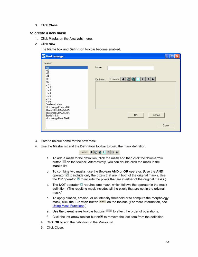
3. Click Close.
To create a new mask 1. Click Masks on the Analysis menu. 2. Click New.
The Name box and Definition toolbar become enabled.
3. Enter a unique name for the new mask. 4. Use the Masks list and the Definition toolbar to build the mask definition.
a. To add a mask to the definition, click the mask and then click the down-arrow
button on the toolbar. Alternatively, you can double-click the mask in the Masks list.
b. To combine two masks, use the Boolean AND or OR operator. (Use the AND operator to include only the pixels that are in both of the original masks. Use the OR operator to include the pixels that are in either of the original masks.)
c. The NOT operator requires one mask, which follows the operator in the mask definition. (The resulting mask includes all the pixels that are not in the original mask.)
d. To apply dilation, erosion, or an intensity threshold or to compute the morphology mask, click the Function button on the toolbar. (For more information, see Using Mask Functions.)
e. Use the parentheses toolbar buttons to affect the order of operations.
f. Click the left-arrow toolbar button to remove the last item from the definition. 4. Click OK to add the definition to the Masks list. 5. Click Close.
83

Using Mask Functions The IDEAS application provides five functions that can be used to create new masks:
• Erode—Removes the selected number of pixels from all edges of the mask.
• Dilate—Adds the selected number of pixels to all edges of the mask.
• Fill—Fills in any holes in the mask.
• Morphology—Includes all pixels within the outermost image contour. This mask, which is used in fluorescence channels, is best used for calculating the values of overall shape-based features.
• Threshold—Adjusts the mask to exclude pixels, based on a percentage of the range of intensity values of the cell (as defined by the original segmentation mask).
The Fill, Erode, and Dilate functions require a mask as input. The Morphology and Threshold functions use the intensity values of a channel image. If you want to use Morphology or Threshold, do not click a mask before clicking the Function toolbar button. If you do click a mask, these functions will not be available.
To insert a function into a mask definition 1. Click Edit to change an existing mask, or click New to create a new mask. 2. Position the cursor in the mask definition where the definition can accept a mask. (This
position exists after an operator in an existing definition or anywhere in a blank definition.) 3. Click the Function button on the toolbar.
The Define Mask Function window appears.
84

4. In the Function list, click the function that you want to apply to the mask. 5. To view a different object in the file, click it in the Object list. 6. To view a different channel image for the object, click the channel in the Channel list. 7. If you are using the Fill, Dilate, or Erode function, click the mask that you want in the
Mask list unless it has already been selected in step 2.. 8. If you are using the Dilate or Erode function, enter the appropriate number in the Number
of Pixels box. 9. If you are using the Morphology or Threshold function, select the channel in the Channel
list. 10. If you are using the Threshold function, set the threshold. 11. Click OK to add the function to the mask definition.
Tip: If a mask function already exists in a mask definition, you can use it as input to a Fill, Dilate, or Erode function.
To use a mask function as an input mask 1. Select function in the Definition box. 2. Click the Function button on the toolbar. The Select Function Mode window
appears.
85
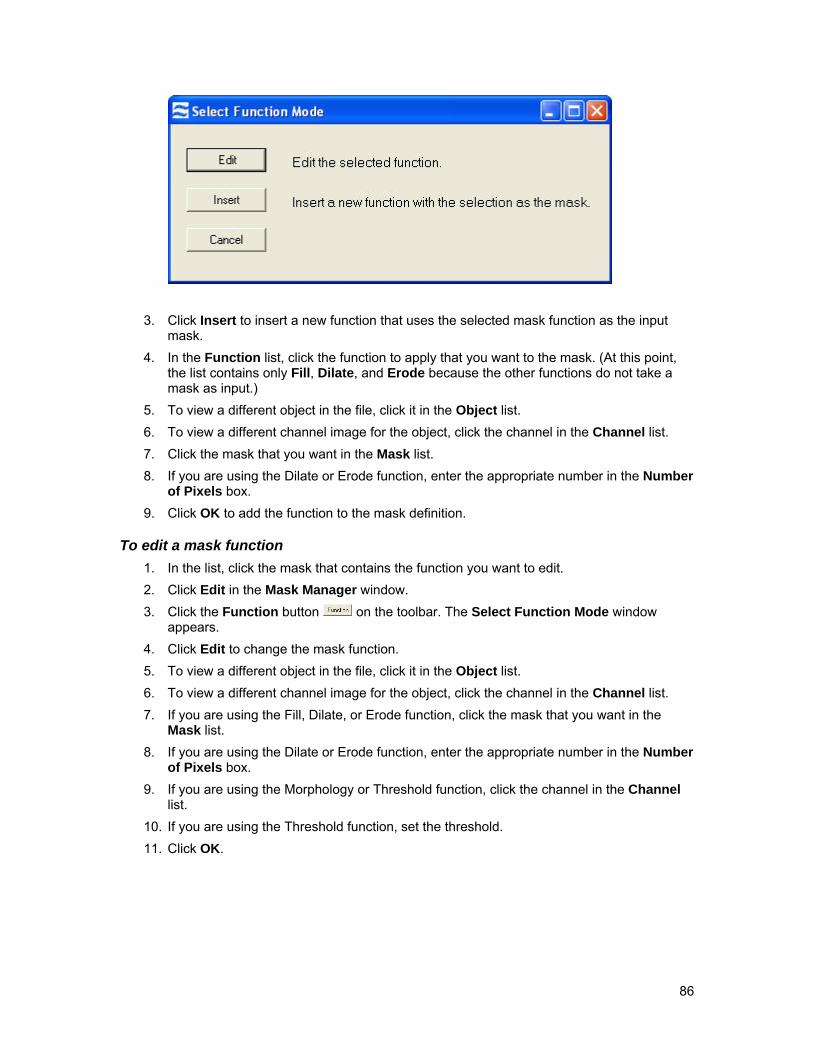
3. Click Insert to insert a new function that uses the selected mask function as the input mask.
4. In the Function list, click the function to apply that you want to the mask. (At this point, the list contains only Fill, Dilate, and Erode because the other functions do not take a mask as input.)
5. To view a different object in the file, click it in the Object list. 6. To view a different channel image for the object, click the channel in the Channel list. 7. Click the mask that you want in the Mask list. 8. If you are using the Dilate or Erode function, enter the appropriate number in the Number
of Pixels box. 9. Click OK to add the function to the mask definition.
To edit a mask function 1. In the list, click the mask that contains the function you want to edit. 2. Click Edit in the Mask Manager window. 3. Click the Function button on the toolbar. The Select Function Mode window
appears. 4. Click Edit to change the mask function. 5. To view a different object in the file, click it in the Object list. 6. To view a different channel image for the object, click the channel in the Channel list. 7. If you are using the Fill, Dilate, or Erode function, click the mask that you want in the
Mask list. 8. If you are using the Dilate or Erode function, enter the appropriate number in the Number
of Pixels box. 9. If you are using the Morphology or Threshold function, click the channel in the Channel
list. 10. If you are using the Threshold function, set the threshold. 11. Click OK.
86

Here is an example of creating a mask of the cytoplasm.
In this example, cells were stained with a green intracellular marker (in Channel 3) and a red nuclear dye (in Channel 5). You can generate a cytoplasm-specific mask by first refining the intracellular and nuclear masks and then removing the nuclear mask pixels from the intracellular mask.
Grayscale Images System Masks (Turquoise Overlay) Channel 3 Channel 5 Mask M3 Mask M5
1. Observe the system masks in the Image Gallery. Since the system masks are designed to capture all the light in an image, they tend to include light that exists beyond the perceived boundaries of the images. In this case, both the intracellular and nuclear masks need to be refined. Start by creating morphology contour masks for both channel images because the Morphology mask is designed to conform to the shape of the image.
2. Click Masks on the Analysis menu. 3. Click New. 4. Click on the Function toolbar button to adjust the mask that will define the whole
cell. The Define Mask Function window appears. 5. Click Morphology in the Function list. Select Channel 3 (intracellular marker). 6. Enter a new mask name, such as Morphology(Intracellular), and click OK to add this
mask to the list. 7. To make the Morphology(Nuclear) mask, repeat steps 3–6 using Channel 5. 8. Click Close. 9. To view the resulting morphology masks, open the Image Display Properties window
and, if necessary, select the new mask for the channel.
10. Next, you will subtract the nuclear morphology mask from the intracellular mask. In the
Mask Manager window, click New. 11. Double-click Morphology(Intracellular) in the Masks list.
12. Click the AND button on the toolbar.
13. Click the NOT button on the toolbar. 14. Double-click Morphology(Nuclear) in the Masks list.
87
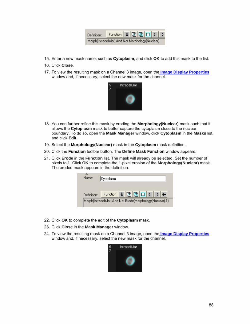
15. Enter a new mask name, such as Cytoplasm, and click OK to add this mask to the list. 16. Click Close. 17. To view the resulting mask on a Channel 3 image, open the Image Display Properties
window and, if necessary, select the new mask for the channel.
18. You can further refine this mask by eroding the Morphology(Nuclear) mask such that it
allows the Cytoplasm mask to better capture the cytoplasm close to the nuclear boundary. To do so, open the Mask Manager window, click Cytoplasm in the Masks list, and click Edit.
19. Select the Morphology(Nuclear) mask in the Cytoplasm mask definition. 20. Click the Function toolbar button. The Define Mask Function window appears. 21. Click Erode in the Function list. The mask will already be selected. Set the number of
pixels to 1. Click OK to complete the 1-pixel erosion of the Morphology(Nuclear) mask. The eroded mask appears in the definition.
22. Click OK to complete the edit of the Cytoplasm mask. 23. Click Close in the Mask Manager window. 24. To view the resulting mask on a Channel 3 image, open the Image Display Properties
window and, if necessary, select the new mask for the channel.
88
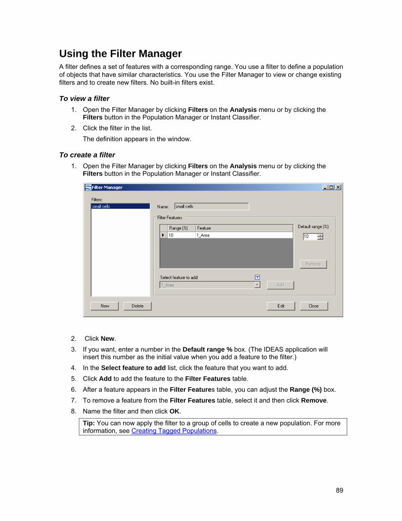
Using the Filter Manager A filter defines a set of features with a corresponding range. You use a filter to define a population of objects that have similar characteristics. You use the Filter Manager to view or change existing filters and to create new filters. No built-in filters exist.
To view a filter 1. Open the Filter Manager by clicking Filters on the Analysis menu or by clicking the
Filters button in the Population Manager or Instant Classifier. 2. Click the filter in the list.
The definition appears in the window.
To create a filter 1. Open the Filter Manager by clicking Filters on the Analysis menu or by clicking the
Filters button in the Population Manager or Instant Classifier.
2. Click New. 3. If you want, enter a number in the Default range % box. (The IDEAS application will
insert this number as the initial value when you add a feature to the filter.) 4. In the Select feature to add list, click the feature that you want to add. 5. Click Add to add the feature to the Filter Features table. 6. After a feature appears in the Filter Features table, you can adjust the Range (%) box. 7. To remove a feature from the Filter Features table, select it and then click Remove. 8. Name the filter and then click OK.
Tip: You can now apply the filter to a group of cells to create a new population. For more information, see Creating Tagged Populations.
89
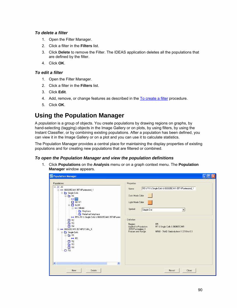
To delete a filter 1. Open the Filter Manager. 2. Click a filter in the Filters list. 3. Click Delete to remove the Filter. The IDEAS application deletes all the populations that
are defined by the filter. 4. Click OK.
To edit a filter 1. Open the Filter Manager. 2. Click a filter in the Filters list. 3. Click Edit. 4. Add, remove, or change features as described in the To create a filter procedure. 5. Click OK.
Using the Population Manager A population is a group of objects. You create populations by drawing regions on graphs, by hand-selecting (tagging) objects in the Image Gallery or on plots, by using filters, by using the Instant Classifier, or by combining existing populations. After a population has been defined, you can view it in the Image Gallery or on a plot and you can use it to calculate statistics.
The Population Manager provides a central place for maintaining the display properties of existing populations and for creating new populations that are filtered or combined.
To open the Population Manager and view the population definitions 1. Click Populations on the Analysis menu or on a graph context menu. The Population
Manager window appears.
90

Note: The list of populations is presented as a hierarchy that shows the dependencies of the populations on each other. The icon associated with a population indicates how the population is defined. The icon indicates the All population or a population defined by a filter. The icon indicates a tagged population. A population defined by a region is indicated by one of the icons. The definition of a selected population is shown in the Definition area.
To edit the display properties of a population 1. Click a population in the Populations list. 2. Change the name in the Name box. 3. Click a Color square to change the display color. Click a new color on the color palette. 4. Click a display symbol in the Symbol list. 5. Click Close to save the population changes. 6. Click Revert to reject the changes.
To delete a population 1. Click a population in the Populations list. 2. Click Delete. A warning message appears indicating all the dependent populations that will
also be deleted. 3. Click OK.
To create a new combined population 1. Click New. The right side of the Population Manager window changes to allow you to
define a new population.
91
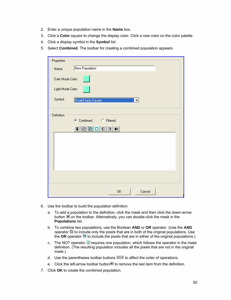
2. Enter a unique population name in the Name box. 3. Click a Color square to change the display color. Click a new color on the color palette. 4. Click a display symbol in the Symbol list. 5. Select Combined. The toolbar for creating a combined population appears.
6. Use the toolbar to build the population definition. a. To add a population to the definition, click the mask and then click the down-arrow
button on the toolbar. Alternatively, you can double-click the mask in the Populations list.
b. To combine two populations, use the Boolean AND or OR operator. (Use the AND operator to include only the pixels that are in both of the original populations. Use the OR operator to include the pixels that are in either of the original populations.)
c. The NOT operator requires one population, which follows the operator in the mask definition. (The resulting population includes all the pixels that are not in the original mask.)
d. Use the parentheses toolbar buttons to affect the order of operations.
e. Click the left-arrow toolbar button to remove the last item from the definition. 7. Click OK to create the combined population.
92

To create a new filtered population 1. Click New. The right side of the Population Manager window changes to allow you to
define a new population. 2. Enter a unique population name in the Name box. 3. Click a Color square to change the display color. Click a new color on the color palette. 4. Click a display symbol in the Symbol list. 5. Select Filtered. The Definition area changes to allow you to create a filtered population.
6. Select Single object or Multiple objects. Then select the object(s) to base the filter on. These object(s) should be the ones that you want the resulting population to match. If you select Multiple objects, the range of the filter in the filter definition will be a percentage of the mean for those objects.
7. Click the filter to use in the Filter list. If a filter does not exist, click Filters to create one. 8. Click the population to filter in the Population to filter list. 9. Click OK to create the filtered population.
93
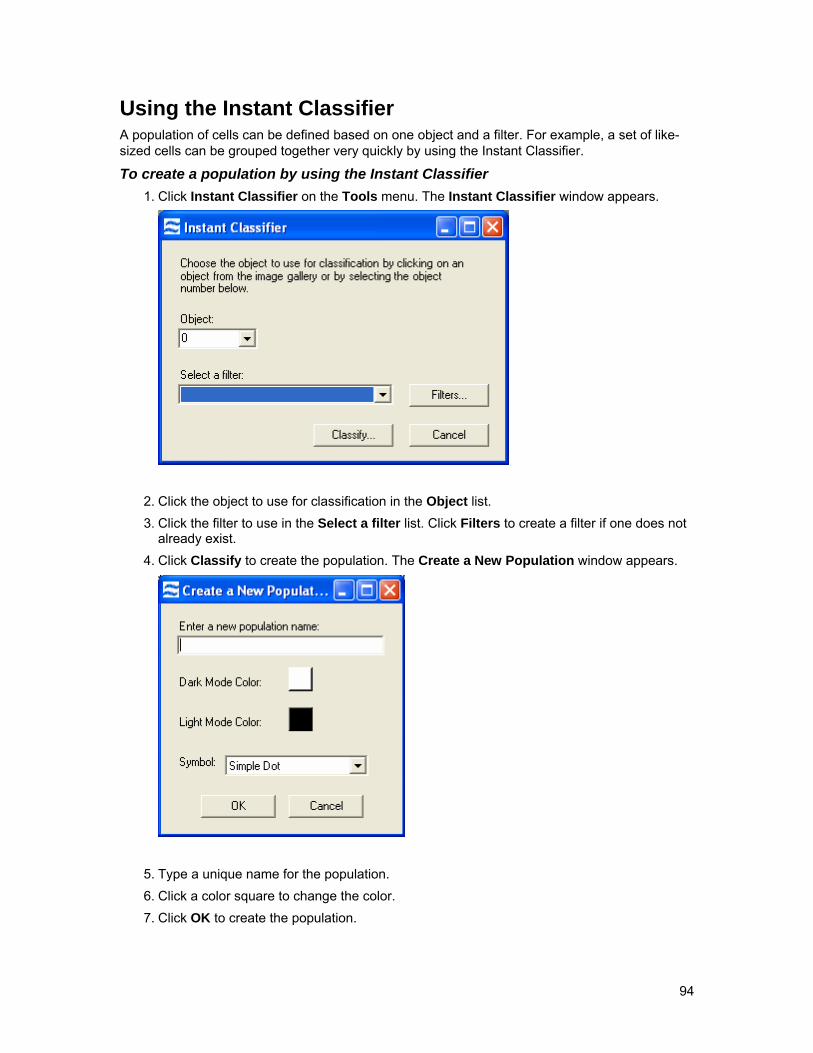
Using the Instant Classifier A population of cells can be defined based on one object and a filter. For example, a set of like-sized cells can be grouped together very quickly by using the Instant Classifier.
To create a population by using the Instant Classifier 1. Click Instant Classifier on the Tools menu. The Instant Classifier window appears.
2. Click the object to use for classification in the Object list. 3. Click the filter to use in the Select a filter list. Click Filters to create a filter if one does not
already exist. 4. Click Classify to create the population. The Create a New Population window appears.
5. Type a unique name for the population. 6. Click a color square to change the color. 7. Click OK to create the population.
94

Creating Reports
The following subsections describe how you can print data directly from the IDEAS application or export data to other applications, such as those in Microsoft Office:
Printing Reports
Exporting Data
Printing Reports The IDEAS application provides color mapping from the dark mode that you see in the Analysis Area to a light mode that has a white background for the printing and exporting of data. Because the population colors might not show on a white background, you can change the colors when using the light mode.
To print the Analysis Area data
• Click Print Analysis Area on the Reports menu. The IDEAS application prints all the graphs, statistics, text panels, and images that are displayed in the Analysis Area.
To print the Image Gallery data
• Click Print Image Gallery on the Reports menu. The IDEAS application prints all the images that are visible in the Image Gallery.
To map the dark mode colors to light mode colors
1. Click Color Scheme Management on the Analysis menu. The Modify Reporting Color Scheme window appears.
2. In the Dark Mode Color list, click the color that you want to map. 3. To choose a different color, click the Select Light Mode Color Mapping color square.
Click a new color on the color palette. 4. Click Update All Populations. 5. If you want to return the settings to the IDEAS defaults, click Reset to Standard. 6. Click OK to save the changes.
95

To print an individual graph 1. Right-click the graph and then click Print Graph on the graph context menu.
The Print Graph window appears.
2. Select Graph and/or Statistics to include the graph and/or statistics in the report. 3. The graph is shown in light mode. Click Customize to change the color mapping for any
of the populations on the graph. Doing so will expand or contract the Print Graph window to show or hide the Color Mapping area.
96
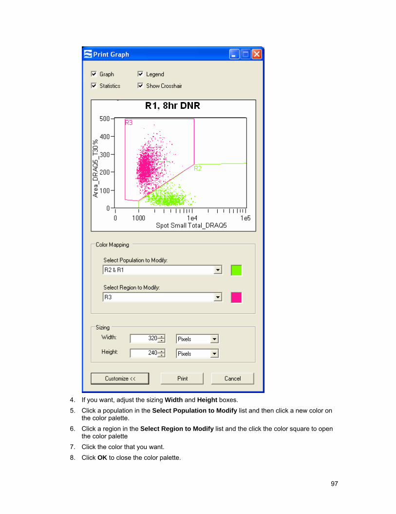
4. If you want, adjust the sizing Width and Height boxes. 5. Click a population in the Select Population to Modify list and then click a new color on
the color palette. 6. Click a region in the Select Region to Modify list and the click the color square to open
the color palette 7. Click the color that you want. 8. Click OK to close the color palette.
97

9. Click OK to print the graph.
Exporting Data You can export graphs, statistics, and images to other applications.
To copy the Image Gallery data to the Clipboard
• Right-click anywhere in the Image Gallery and then click Copy Displayed Images to Clipboard. The IDEAS application copies all the images that are visible in the Image Gallery to the Clipboard.
To copy a single image to the Clipboard
• Right-click an image in the Image Gallery or in the Analysis Area and then click Copy Image to Clipboard.
To copy a graph to the Clipboard 1. Right-click a graph and then click Copy Graph/Stats to Clipboard. The Copy
Graph/Statistics window appears.
2. Select Graph, Statistics and/or Legend depending on what you want to copy. 3. Click Customize to change the color mapping of any of the populations on the graph.
Doing so expands the window to show the Color Mapping area.
98

4. Click a population in the Select Population to Modify list and then click a new color on
the color palette. 5. Click the color that you want. 6. Click OK to close the color palette. 7. If you want to copy the graph in dark mode (as it appears in the Analysis Area), select
Dark Mode. 8. Click Copy to copy the graph and/or the statistics to the Clipboard.
Note: The IDEAS application copies the statistics as a metafile. If you want to export the data into a table, such as that in Microsoft Excel, you must instead click Export Statistics to Clipboard on the context menu.
99

To export graph statistics to the Clipboard
• Right-click a graph and then click Export Statistics to Clipboard.
To export statistics, feature data, or the compensation matrix from the Statistics Area
• Right-click the table and then click Copy Data to Clipboard.
To copy the entire screen to the Clipboard
• Press CTRL+PRINT SCREEN.
To copy a window to the Clipboard
• Select the window and then press ALT+PRINT SCREEN.
100
Understanding the IDEAS® Features
This section contains the following subsections, which describe the features that the IDEAS application uses for data analysis:
Overview of the IDEAS® Features
The Base Features at a Glance
Understanding the Detailed Feature Descriptions
Understanding the Size Features
Understanding the Location and Shape Features
Understanding the Signal Strength Features
Understanding the Shape and Texture Features
Understanding the Spot Features
Understanding the Object Information Features
Understanding the Comparison Features
101

Overview of the IDEAS® Features Objects passing through the ImageStream cell analysis system are illuminated in different directions by lasers and/or a halogen lamp. Light emitted from the object is focused through an objective lens and relayed to a spectral decomposition element, which divides the light into six spectral bands located side-by-side across a charge-coupled detector (CCD), as shown in the following diagram. Each object therefore has six images that can be individually analyzed or, because they are in spatial register with respect to one another, reconstructed. Each of the separate bands is called a channel. Each channel produces an image over time, with the sensitivity of the detection increasing.
The IDEAS application provides a large selection of criteria, or features, for analyzing images. A feature is described by a mathematical expression that contains quantitative and positional information about the image. A few object features, such as Object Number and Flow Speed, do not require calculations, masks, or image intensity information.
A feature is characterized as a single feature or a combined feature. A single feature uses a base feature, such as Area or Total Intensity, along with a mask and/or a channel. A combined feature is created by a mathematical expression that includes one or more single features.
You can combine existing features into new features by using the Feature Manager. You can also create new masks that you can then use to generate new features by using the Mask Manager. (For more information, see Using the Feature Manager and Using the Mask Manager.)
To calculate the value of a feature, the IDEAS application maps the channel image to X and Y coordinates, as illustrated by the following diagram. Each box in the diagram represents a pixel
102

that equals approximately 0.5 µm × 0.5 µm. Each channel is 88 pixels in the X direction and varies in the Y direction, depending on the size of the imaged object.
The set of pixels that contains the region of interest is called the mask and is specific to each channel image. In the following diagram, the mask consists of the set of pixels that are light and dark blue. The object is represented by the dark blue pixels. Calculating some feature values, such as the Area value, requires only a mask. Calculating others, such as the Mean Intensity value, requires a mask and intensity values.
The IDEAS application determines the mask by a process called segmentation. The segmentation algorithm searches for pixels that have signal strengths above those of the background, and the algorithm then creates a closed, filled-in shape. It may appear to the eye that the edge of the object is well within the bounds of the mask. The following figure contains an example of an unmasked image next to the same image with its channel mask.
You can use the Feature Manager to combine masks from different channels. The IDEAS application provides a combined mask that is the union of the pixels from all six channel masks.
0, 0
X
8, 0
Y
0, 8
103
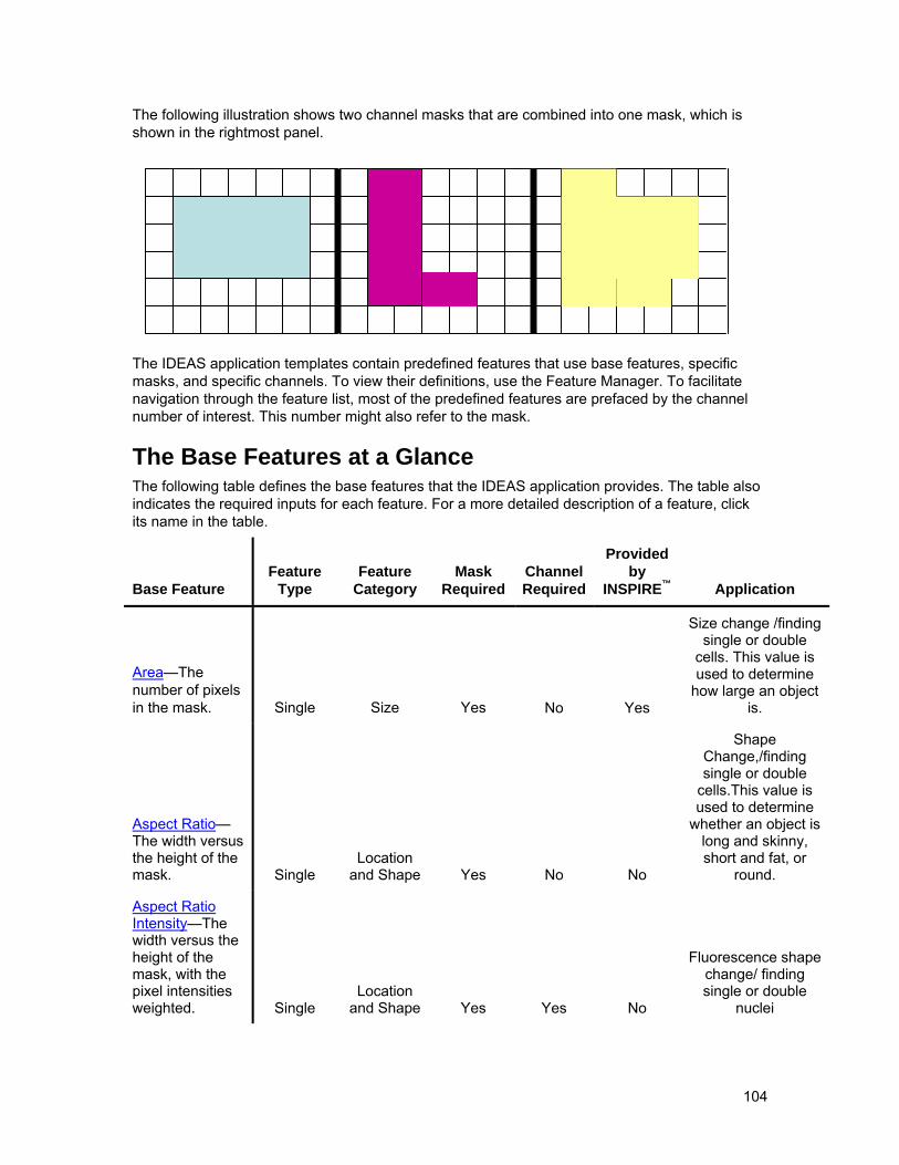
The following illustration shows two channel masks that are combined into one mask, which is shown in the rightmost panel.
The IDEAS application templates contain predefined features that use base features, specific masks, and specific channels. To view their definitions, use the Feature Manager. To facilitate navigation through the feature list, most of the predefined features are prefaced by the channel number of interest. This number might also refer to the mask.
The Base Features at a Glance The following table defines the base features that the IDEAS application provides. The table also indicates the required inputs for each feature. For a more detailed description of a feature, click its name in the table.
Base Feature Feature
Type Feature
Category Mask
Required Channel Required
Provided by
INSPIRE™ Application
Area—The number of pixels in the mask. Single Size Yes No Yes
Size change /finding single or double
cells. This value is used to determine
how large an object is.
Aspect Ratio—The width versus the height of the mask. Single
Location and Shape Yes No No
Shape Change,/finding single or double
cells.This value is used to determine
whether an object is long and skinny, short and fat, or
round.
Aspect Ratio Intensity—The width versus the height of the mask, with the pixel intensities weighted. Single
Location and Shape Yes Yes No
Fluorescence shape change/ finding single or double
nuclei
104

Base Feature Feature
Type Feature
Category Mask
Required Channel Required
Provided by
INSPIRE™ Application
Background Mean Intensity—The average intensity of the background of an image outside of the combined mask. Single
Signal Strength Yes Yes No
Measures channel background,
calculates signal over background. This value can be subtracted from
intensity measurements (for more information,
see Intensity).
Background StdDev Intensity—The standard deviation of the background intensities. Single
Signal Strength Yes Yes No
Measures channel noise
Camera Line Number—The line number assigned by the camera. This number might wrap in a large data file. Single Object No No No
This value can be used to distinguish individual data files when multiple files have been merged
Camera Timer—A time stamp assigned by the camera for the object. Single Object No No No
This value can be used to calculate
sample concentration and duration of sample
run.
Centroid X—The central tendency along the X Axis of the pixels that are within the mask. Single
Location and Shape Yes No No
This value can be used to determine
the horizontal location of an object relative to the entire
image.
105

Base Feature Feature
Type Feature
Category Mask
Required Channel Required
Provided by
INSPIRE™ Application
Centroid X Intensity—The central tendency of the pixels along the X Axis, with the pixel intensities weighted. Single
Location and Shape Yes Yes No
This value tends to move horizontally
toward the brightest pixels in the image and can be used to
calculate radial delta centroid to find
TUNEL artifacts, capped
fluorescence, or polarization.
Centroid Y—The central tendency along the Y Axis of the pixels that are within the mask. Single
Location and Shape Yes No No
This value can be used to determine
the vertical location of an object relative to the entire image and can be used to
find images with multiple objects.
Centroid Y Intensity—The central tendency of the pixels along the Y Axis, with the pixel intensities weighted. Single
Location and Shape Yes Yes No
This value tends to move vertically
toward the brightest pixels in the image and can be used to
calculate radial delta centroid to find
TUNEL artifacts, capped
fluorescence, or polarization.
Combined Mask Intensity—The total intensity of all the pixels that are included in the combined mask. Single
Signal Strength Yes Yes No Immunophenotyping
Compactness—The degree of circularity of the object. Single Shape No Yes No
106

Base Feature Feature
Type Feature
Category Mask
Required Channel Required
Provided by
INSPIRE™ Application
Elongatedness—The width versus the height of the mask. Single Shape No Yes No
This value, which is similar to Aspect Ratio, is used to
determine whether an object is long and skinny, short and fat, or round.
Flow Speed—The flow speed of the object when it was collected. Single Object No No No
This value is used to normalize the
intensities among objects that are due
to changes in the flow speed of the
instrument.
Frequency—The overall distribution of the pixel intensities. Single
Shape and Texture Yes Yes No
Texture changes in apoptosis
Gradient Max—The point of sharpest focus in the image. Single
Shape and Texture Yes Yes No
To identify focused cells
Gradient RMS—The overall focus of the image. Single
Shape and Texture Yes Yes No
To identify focused cells
Intensity—The total pixel intensity of an object, with the background subtracted. Combined
Signal Strength Yes Yes No Immunophenotyping
Major Axis—The length of the widest part of the mask. Single
Location and Shape Yes No No Shape change
Major Axis Intensity—The length of widest part of the mask, with the pixel intensities weighted. Single
Location and Shape Yes Yes No
Target shape change
107

Base Feature Feature
Type Feature
Category Mask
Required Channel Required
Provided by
INSPIRE™ Application
Mean Intensity—The average pixel intensity. This value indicates the overall brightness of the object. Single
Signal Strength Yes Yes No
Used in combination with Peak Intensity
to look for internalization.
Minimum Intensity—The smallest pixel intensity for the object. Single
Signal Strength Yes Yes Yes
Chromometric absorbance,
identifies melanin content or malaria
infected cells
Minor Axis—The length of the narrowest part of the mask. Single
Location and Shape Yes No No
This value can be used to measure
cell diameter for cell size assays.
Minor Axis Intensity—The length of the narrowest part of the mask, with the pixel intensities weighted. Single
Location and Shape Yes Yes No
This value can be used to measure
fluorescence diameter for cell
size assays.
Negative Curvatures—The jaggedness of the object’s shape. Single Shape No Yes No
Object Rotation Angle—The angle of the object’s major axis relative to the horizontal plane. Single
Location and Shape Yes No No
This value can be used to determine
the orientation of an object, especially if the object is oblong.
108

Base Feature Feature
Type Feature
Category Mask
Required Channel Required
Provided by
INSPIRE™ Application
Object Rotation Angle Intensity—The angle of the object’s intensity-weighted major axis relative to the horizontal plane. Single
Location and Shape Yes Yes No
Measures the orientation of oblong
fluorescence of hydrodynamically
focused cells in the core stream
Peak Intensity—The largest pixel intensity of the object. Single
Signal Strength Yes Yes Yes
Identifies saturated events that are
improperly compensated
Perimeter—The circumference of the mask. Single Size Yes No No
Shape and volume change assays
Similarity Single Comparison Yes Yes No
Comparing two channel images for
translocation assays
Similarity Bright Detail Single Comparison Yes Yes No
Comparing the brightest details of
the images in 2 channels for co-localization or
translocation assays
Spot Count—The number of disconnected regions that are present in a mask. Single
Location and Shape Yes Yes No FISHIS
Spot Small Max—In an image that is less than 7 pixels wide, the largest difference in spot intensity from the background. Single
Shape and Texture No Yes No
109
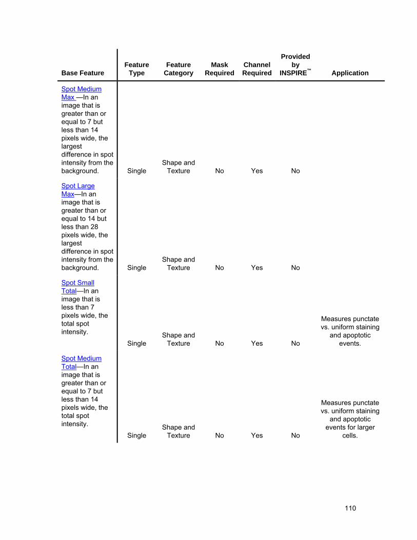
Base Feature Feature
Type Feature
Category Mask
Required Channel Required
Provided by
INSPIRE™ Application
Spot Medium Max —In an image that is greater than or equal to 7 but less than 14 pixels wide, the largest difference in spot intensity from the background. Single
Shape and Texture No Yes No
Spot Large Max—In an image that is greater than or equal to 14 but less than 28 pixels wide, the largest difference in spot intensity from the background. Single
Shape and Texture No Yes No
Spot Small Total—In an image that is less than 7 pixels wide, the total spot intensity.
Single Shape and
Texture No Yes No
Measures punctate vs. uniform staining
and apoptotic events.
Spot Medium Total—In an image that is greater than or equal to 7 but less than 14 pixels wide, the total spot intensity.
Single Shape and
Texture No Yes No
Measures punctate vs. uniform staining
and apoptotic events for larger
cells.
110
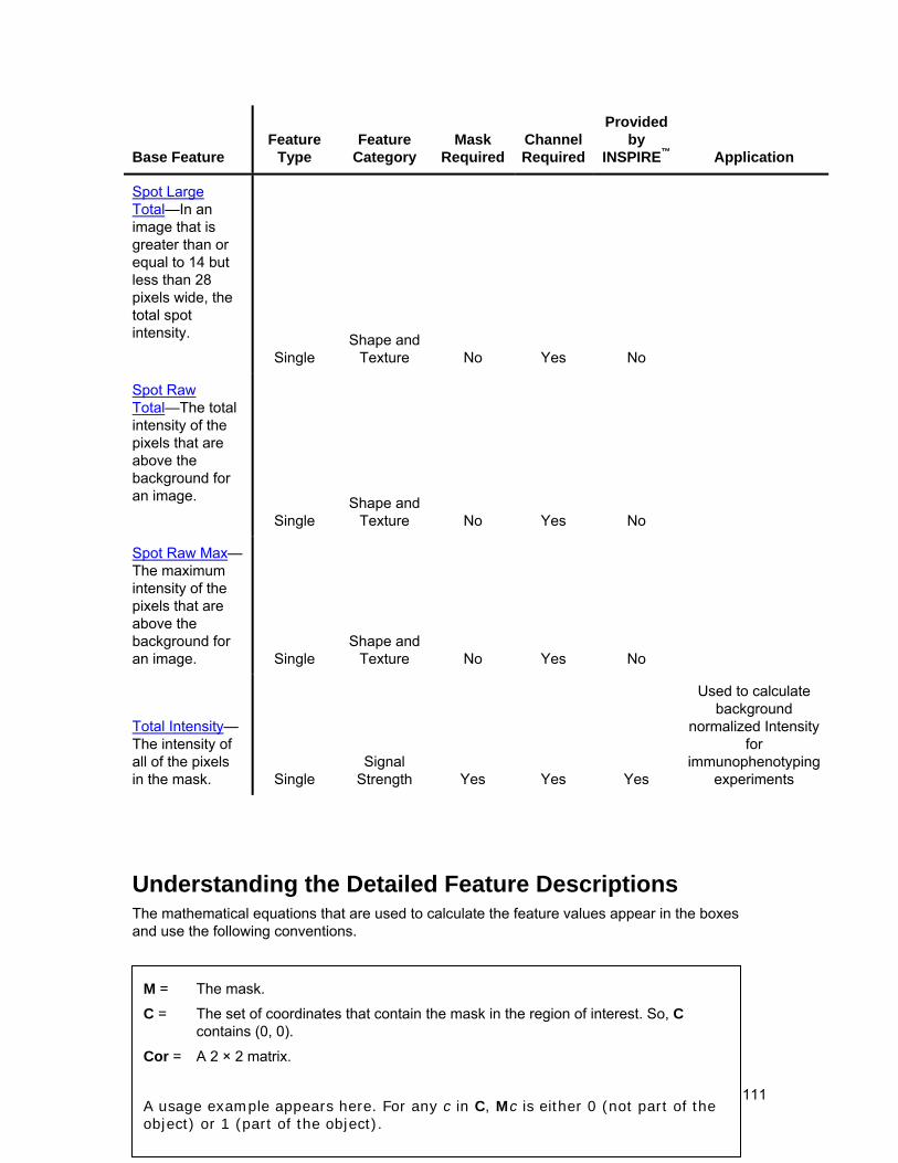
Base Feature Feature
Type Feature
Category Mask
Required Channel Required
Provided by
INSPIRE™ Application
Spot Large Total—In an image that is greater than or equal to 14 but less than 28 pixels wide, the total spot intensity.
Single Shape and
Texture No Yes No
Spot Raw Total—The total intensity of the pixels that are above the background for an image.
Single Shape and
Texture No Yes No
Spot Raw Max—The maximum intensity of the pixels that are above the background for an image. Single
Shape and Texture No Yes No
Total Intensity—The intensity of all of the pixels in the mask. Single
Signal Strength Yes Yes Yes
Used to calculate background
normalized Intensity for
immunophenotyping experiments
Understanding the Detailed Feature Descriptions The mathematical equations that are used to calculate the feature values appear in the boxes and use the following conventions.
M = The mask.
C = The set of coordinates that contain the mask in the region of interest. So, C contains (0, 0).
Cor = A 2 × 2 matrix.
A usage example appears here. For any c in C, Mc is either 0 (not part of the object) or 1 (part of the object).
111

Understanding the Size Features The Area Feature The number of pixels in a mask is equal to the Area. The segmentation equation takes the intensity values from each pixel and includes (as a value of 1) or excludes (as a value of 0) that pixel from the Area calculation. The criterion for inclusion is the set of intensity values above a certain threshold value, which may or may not be visible to the eye. This criterion means that the mask is usually a bit larger than the image appears.
The Area value is determined by counting the number of nonzero bits in the mask:
Area = 0
For each c in C:
Area += Mc
In the following figure, the pixels are not drawn to scale and are for illustration purposes only:
This image’s mask is equal to approximately 42 pixels. Note that some overlap exists into pixels that are not included, and some pixels are included that do not appear to have signal to the eye. The latter inclusion depends on the mask definition.
The Area is related to the size of the cell. Note that 1 pixel = 0.25 µm2. A round cell with a mask that has a 50-pixel diameter has an area of 1963 pixels and is therefore equal to 491 µm2.
The Perimeter Feature The number of pixels that surround the mask is equal to the Perimeter.
The Perimeter is determined by the following steps:
1. Dilate the mask M using a 3 × 3 dilation kernel. 2. Perform the XOR operation on the dilated mask and the original mask, and store
the result in, let’s say, XMask. 3. Count the number of nonzero bits in XMask.
112

In the following figure, the yellow pixels surround the blue mask, and the Perimeter value is 26 pixels.
4 4
8, 0 0, 0
0, 8
The Perimeter value is an indication of size.
Understanding the Location and Shape Features The Aspect Ratio Feature The Aspect Ratio is the Minor Axis divided by the Major Axis of the mask that is rotationally independent.
majAR λ
λmin=
The Aspect Ratio Intensity Feature The Aspect Ratio Intensity is the Minor Axis Intensity divided by the Major Axis Intensity. The following figure illustrates the axes:
113

Major Axis
Minor Axis
The relative shape and size of objects can be deduced from these measurements. Two cells in a frame or exceptionally large or small cells can be detected.
The Centroid X and Centroid Y Features Centroid location is a measurement of the central tendency of the mask within the channel along the X or Y Axis. The value represents the pixel location of the center of the mask.
Given the mask M, Centroid X (Cx) and Centroid Y (Cy) are defined by:
N
jC Mji
y
∑∈= ),(
N
iC Mji
x
∑∈= ),(
and
Im refers to the image.
114
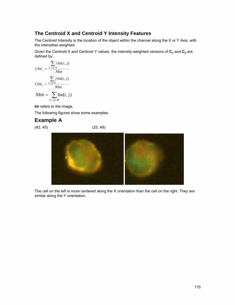
The Centroid X and Centroid Y Intensity Features The Centroid Intensity is the location of the object within the channel along the X or Y Axis, with the intensities weighted.
Given the Centroid X and Centroid Y values, the intensity-weighted versions of Cx and Cy are defined by:
NInt
iCInt Mji
x
∑∈= ),(
Im( ji ),
NInt
jijCInt Mji
y
∑∈= ),(
),Im(
∑∈
=Mji
jiNInt),(
),Im(
Im refers to the image.
The following figures show some examples.
Example A (42, 45) (25, 48)
x x
The cell on the left is more centered along the X orientation than the cell on the right. They are similar along the Y orientation.
115
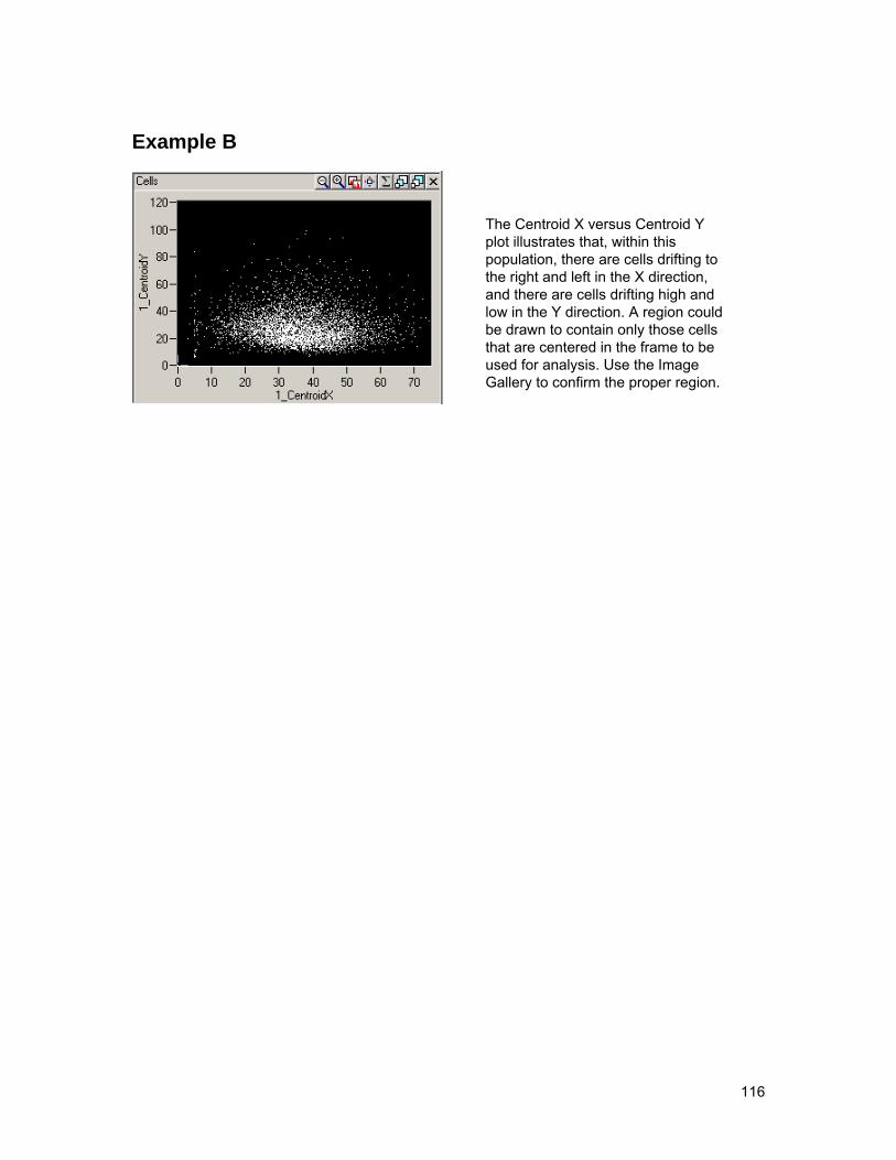
Example B
The Centroid X versus Centroid Y plot illustrates that, within this population, there are cells drifting to the right and left in the X direction, and there are cells drifting high and low in the Y direction. A region could be drawn to contain only those cells that are centered in the frame to be used for analysis. Use the Image Gallery to confirm the proper region.
116
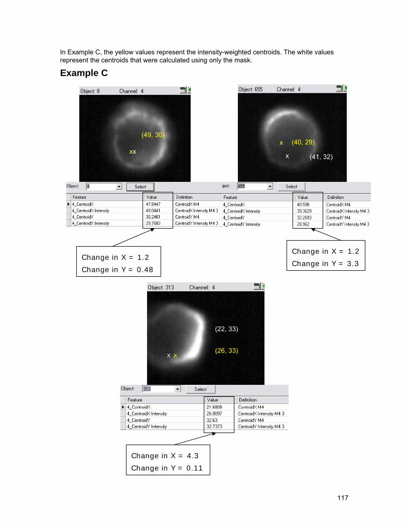
In Example C, the yellow values represent the intensity-weighted centroids. The white values represent the centroids that were calculated using only the mask.
Example C
(48, 30) (49, 30) (40, 29) x
xx x (41, 32)
Change in X = 1.2
Change in Y = 3.3 Change in X = 1.2
Change in Y = 0.48
(22, 33)
(26, 33) X X
Change in X = 4.3
Change in Y = 0.11
117
You can use centroid measurements to determine relative positional locations. You can also use these measurements to eliminate objects on the edges of the channel in the X direction or to eliminate multiple objects in the Y direction, which tend to have longer channel images due to their size.
The Elongatedness Feature Elongatedness is a shape feature, similar to aspect ratio. It can be used to identify bean-like cells from circular cells. For simplicity, it can be thought of as the inverse of aspect ratio. More specifically, Elongatedness is defined as the ratio of the maximum width to the minimum width of the bounding rectangle of the object.
Equations:
Elongatedness E is computed as follows:
)(( )∆
∆
−+
++=
YYXX
YYXXEσσσσ ,
where for all N points {CX, CY}i on the perimeter of the object (typically, the object is specified by the morphology mask),
∑∑==
==N
iYY
N
iXX ii
CN
CN 11
1,1 µµ ,
( )( )∑=
−−=N
iXXXXXX ii
CCN 1
1 µµσ , ( )( )∑=
−−=N
iYYXXXY ii
CCN 1
1 µµσ ,
( )( )− YYY iC µµ∑
=
−=N
iYYY i
CN 1
1σ
( )
, and
( )22 4 XYYYXXYYXX σσσσσ −−+=∆
Applications: Elongatedness has a lower bound of 1 which indicates a perfect circular shape. The larger the value, the more bean-like the shape. Typically, values greater than 1.5 indicate elongated shapes, so this is a very sensitive measure, unlike the aspect ratio. For more robust results, it is best to combine this feature with the aspect ratio of the morph mask to isolate bean-like shapes from circular ones.
The Major Axis Feature The longest diameter of an object’s mask is the Major Axis, and it is approximately +/− one standard deviation from the centroid in the longest direction of the object. The units are pixels.
118

The Minor Axis Feature The shortest diameter of an object’s mask is the Minor Axis, and it is approximately +/− one standard deviation from the centroid in the shortest direction of the object. The units are pixels.
First, th ollowing variables are defined: e fN
CiC Mi
x
xx
∑∈
−)
)(j= ,(
2
N
CjC Mji
y
yy
∑∈
−= ),(
2)(
N
CjCiC Mji
yx
xy
∑∈
−−= ),(
))((
⎥⎦
⎤⎢⎣
⎡=
yyxy
xyxx
CCCC
A
majλminλ
Then, the following 2 × 2 matrix A is constructed:
Then, the values of the major and minor axes are the major ( ) and minor ( ) Eigen values, respectively. Then, the value of the Aspect Ratio (AR) is:
majAR λ
λmin=
The Major Axis Intensity Feature The Major Axis Intensity is weighted by intensity measurements as well as by the location and will be influenced by an off-center area with high or low intensities.
119
The Minor Axis Intensity Feature The Minor Axis Intensity is weighted by intensity measurements as well as by the location and will be influenced by an off-center area with high or low intensities.
The intensity-weighted versions of the Major Axis, Minor Axis, Aspect Ratio, and Object Rotation Angle are almost identical with the following exceptions:
NInt
ji 2),Im(CiCInt Mji
x
xx
∑∈
−= ),(
2)(
NInt
j 2),iCjCInt Mji
y
yy
∑∈
−= ),(
2 Im()(
NInt
jiCjCi y2),Im())((∑ −−
CInt Mjix
xy),( ∈=
The Negative Curvatures Feature
This is yet another shape measure. It can be used to determine the jaggedness of the contour of a cell. The smoother the contour, the less the value of Negative Curvatures.
Equations: Negative curvatures is measured by counting the number of slope changes along the contour. One negative curvature corresponds to a change from positive to negative and back to positive. For robustness, a minimum threshold is applied to determine a slope change to avoid influence by noise.
Applications: A value of 0 indicates a perfectly convex contour (such as a circle). The bigger this measure, the less convex the object contour (usually defined by the morphology mask), which, in turn, implies that the object counter is more jagged. In most cases, this also indicates a higher circular variance value.
The Object Rotation Angle Feature The angle of the Major Axis from the horizontal plane is the Object Rotation Angle.
The Object Rotation Angle Intensity Feature The angle of the Major Axis Intensity from the horizontal plane is the Object Rotation Angle Intensity.
120
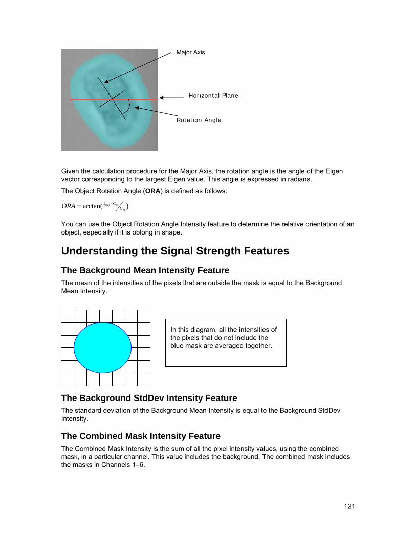
Major Axis
Given the calculation procedure for the Major Axis, the rotation angle is the angle of the Eigen vector corresponding to the largest Eigen value. This angle is expressed in radians.
The Object Rotation Angle (ORA) is defined as follows:
)arctan(xy
xxmajC
CORA −= λ
You can use the Object Rotation Angle Intensity feature to determine the relative orientation of an object, especially if it is oblong in shape.
Understanding the Signal Strength Features The Background Mean Intensity Feature The mean of the intensities of the pixels that are outside the mask is equal to the Background Mean Intensity.
The Background StdDev Intensity Feature The standard deviation of the Background Mean Intensity is equal to the Background StdDev Intensity.
The Combined Mask Intensity Feature The Combined Mask Intensity is the sum of all the pixel intensity values, using the combined mask, in a particular channel. This value includes the background. The combined mask includes the masks in Channels 1–6.
In this diagram, all the intensities of the pixels that do not include the blue mask are averaged together.
Rotation Angle
Horizontal Plane
121
The Intensity Feature The Intensity Feature is a combined feature that uses two base features: Combined Mask Intensity − (Background Mean Intensity × Combined Mask Area).
The Mean Intensity Feature The average intensity of the pixels in the channel mask is the Mean Intensity. The Mean Intensity is also defined by Total Intensity / Area.
The Minimum Intensity Feature The smallest intensity value of a pixel in the channel mask is the Minimum Intensity.
The Peak Intensity Feature The maximum pixel intensity in the channel mask is the Peak Intensity.
The Total Intensity Feature The total of all of the pixel intensity values in the channel mask is the Total Intensity.
You can use the Intensity values to determine the overall brightness of an object. When performing calculations, you can use the Peak Intensity values to discard objects that are sensitive to saturation.
Understanding the Shape and Texture Features The Compactness Feature Compactness is another shape feature. It is used to measure the degree of circularity of a cell. Formally, the compactness is defined as the ratio of the square of the perimeter of the object over the area of the object. The bigger the number, the more complex the object shape. Compactness is a positive number with a lower bound of 4*pi, which is achieved by the perfect circle. For our application, this definition is numerically susceptible to the inaccuracies in the measurement of the contour length (perimeter). Therefore, we adopt a circular variance type of measure, which is a non-negative number that measures how much the object contour varies from the contour of the perfect circle centered at the centroid (CX, CY) of the object and having a radius µ equal to the mean deviation of the object contour from the centroid of the object. Equations: More specifically, Compactness C of an object is given by:
( ) ( )2
1
221 ∑=
⎟⎠⎞⎜
⎝⎛ −−+−
N
iiYiX YCXC
Nµ , =C
where (CX, CY) is the centroid of the object (typically defined by the morphology mask), (Xi ,Yi) are the N points on the perimeter of the object and
( ) ( )2
1
221 ∑=
⎟⎠⎞⎜
⎝⎛ −+−=
N
iiYiX YCXC
Nµ .
122
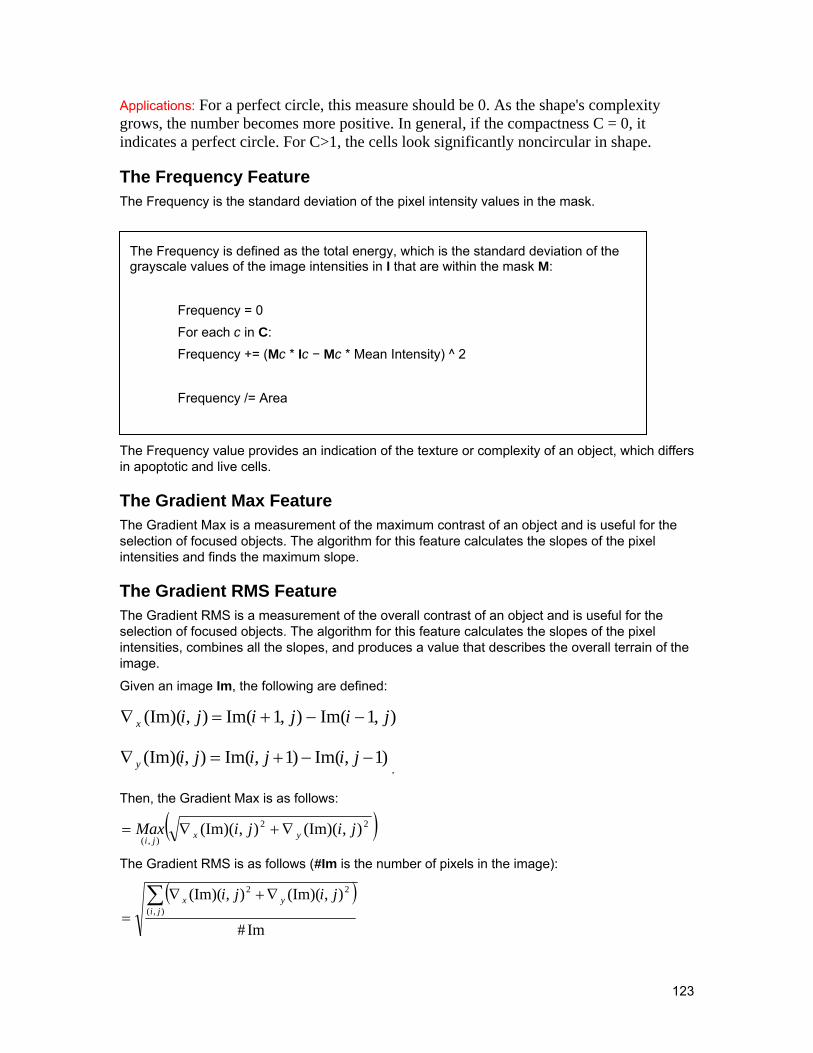
Applications: For a perfect circle, this measure should be 0. As the shape's complexity grows, the number becomes more positive. In general, if the compactness C = 0, it indicates a perfect circle. For C>1, the cells look significantly noncircular in shape.
The Frequency Feature The Frequency is the standard deviation of the pixel intensity values in the mask.
The Frequency is defined as the total energy, which is the standard deviation of the grayscale values of the image intensities in I that are within the mask M: Frequency = 0 For each c in C: Frequency += (Mc * Ic − Mc * Mean Intensity) ^ 2 Frequency /= Area
The Frequency value provides an indication of the texture or complexity of an object, which differs in apoptotic and live cells.
The Gradient Max Feature The Gradient Max is a measurement of the maximum contrast of an object and is useful for the selection of focused objects. The algorithm for this feature calculates the slopes of the pixel intensities and finds the maximum slope.
The Gradient RMS Feature The Gradient RMS is a measurement of the overall contrast of an object and is useful for the selection of focused objects. The algorithm for this feature calculates the slopes of the pixel intensities, combines all the slopes, and produces a value that describes the overall terrain of the image.
Given an image Im, the following are defined:
),1Im(),1Im(),(Im)( jijijix −−+=∇
,Im(),(Im)(
=∇ ijiy )1,Im()1 −−+ jij.
Then, the Gradient Max is as follows:
( )22
),(),(Im)(),(Im)( jijiMax yxji
∇+∇=
( )
The Gradient RMS is as follows (#Im is the number of pixels in the image):
Im#
),(Im)(),(Im)(),(
22∑ ∇+∇= ji
yx jiji
123

The Gradient Max can be used for finding cells that have specific areas of high contrast. The parallel operation in microscopy is focusing on the brightest section of an image.
The Gradient RMS can be used to find the cells that are in the best overall focus. The parallel operation in microscopy is adjusting the fine focus on an image so that the overall focus is the best.
Understanding the Spot Features The Spot Count Feature The Spot Count feature measures the number of connected components or contiguous objects in the mask corresponding to an image.
For each image mask, a connected component is defined as one where all pixels in the image mask have at least one nonzero pixel in the 3 x 3 neighborhood surrounding the pixel.
The Spot Count can be used to count the FISH spots in a cell.
The Spot Small Max, Spot Medium Max, Spot Large Max, Spot Small Total, Spot Medium Total, and Spot Large Total Features These features each subtract the background level from an image and then generate three separate versions of the image, which contain bright objects of small, medium, and large minimum widths. The feature values are statistical descriptions of the intensities that are present in those image versions.
Specifically, small spots are smaller than 7 pixels across, medium spots are larger than 7 and smaller than 14 pixels across, and large spots are larger than 14 and smaller than 28 pixels across. The spot categories do not require their objects to be smaller than the threshold distance along all axes—only along one axis. Thus, a long, narrow image feature that is 20 pixels long but only 4 pixels across contributes to the Small Spot features—not to the Medium or Large Spot features.
124

The Spot Raw Total and Spot Raw Max Features These features each subtract the background level from an image and then provide a statistical description of the intensities that are present in the new image.
The following diagram represents a density plot of an object that has two small high-intensity regions, one surrounded by an area of medium intensity and the other by an area of low intensity:
The small, medium and large regions are delineated by their sizes and combined for calculating the total intensity and maximum intensity:
Intensity
Small Regions of High Intensity
Pixel
Small
Medium
Large
125

The following diagram illustrates a similar image with an additional small spot of higher intensity than its surroundings but of lower total intensity:
The Spot features make use of an image processing technique that is known as mathematical morphology. For more information, see Image Analysis and Mathematical Morphology, Vol. 1, J. Serra (Academic Press, 1982).
The opening kernels use the following kernel:
0011100
0111110
1111111
1111111
1111111
0111110
0011100
Down sampling is defined as follows:
)12,12Im()12,2Im()2,12Im()2,2Im()),(Im( +++++++= ijijij jijiDS
∑∈
=Br
rijiBE ),Im(),(Im)(
DS(Im) is now an image that is half the width and height (or one quarter of the size) of Im.
Background estimation is defined as follows:
B = {0, 1, 2, 3, H−4, H−3, H−2, H−1}, which are the first and last four rows of Im. Thus, BE(Im)(i, j) is a function of only the columns i. The following diagram contains the spot image processing algorithm:
126

Im
Background Estimator
Opening
Raw Spot Image
Small Spot Image
Down Sample
Opening Medium Spot Image
Down Sample
Opening Large Spot Image
The Total and Max features are based on the image-processing outputs: raw spot image, small spot image, medium spot image, and large spot image. Given one of these images, named SIP, the feature equations are as follows:
∑=),(
),(ji
jiSIPTotal
),(),(
jiSIPMaxMaxji
=
127
Understanding the Object Information Features The Camera Line Number Feature The Camera Line Number is the line number assigned by the camera as the object is detected.
The Camera Timer Feature The Camera Timer is the clock rate, in KHz, during acquisition. This value is relative time.
The Flow Speed Feature The Flow Speed is the calculated flow speed, in Hz, of the object.
The Object Number Feature The Object Number represents the sequence of objects in the .cif file.
Understanding the Comparison Features The Similarity Feature The Similarity is a measure of the degree to which two images are linearly correlated within a masked region.
One problem with the use of Pearson's correlation coefficient in practical experiments is that, when images are at all similar, the values tend to pile up near 1 and the variations within a sample do not follow a normal distribution. To allow the use of parametric statistics on a measure of linear image similarity, the similarity score s is defined in terms of the correlation coefficient as follows:
⎥⎦
⎤⎢⎣
⎡−+
=ρρ
11lns
This definition expands the theoretical range of values to the full real number line. In practice, the definition brings many samples of objects into close agreement with a normal distribution. For these reasons, the use of the Similarity value is recommended in most cases.
The Normalized Similarity Feature The Normalized Similarity value is like the Similarity value, but it has a range between −1 and 1. It is actually the Pearson's correlation coefficient of the gray levels of the images within the masked region. The Normalized Similarity value is the Pearson's correlation coefficient that is calculated between the gray levels of the masked pixels of two images. Specifically, the equation for the correlation coefficient ρ is as follows:
∑ ∑
∑−−
−−=
i jji
iii
YyXx
YyXx
22 )()(
))((ρ
In the equation, xi and yi are the per-pixel gray levels of the two images in the masked region and X and Y are the corresponding mean gray levels in the masked region. The correlation coefficient provides a measure of the degree to which two sets of data tend to be linearly related. Positive
128
linear relationships give positive coefficients, whereas negative relationships give negative coefficients. The correlation coefficient varies from −1 to 1. Before calculating a Similarity value, it is important to make sure that the mask contains the pixels—and only the pixels—over which the Similarity ought to be measured. In particular, the presence of background or near-background pixels in a mask may corrupt the results of the measurement by inducing spurious correlations (pixel values being correlated by virtue of merely being both inside and outside the object).
The Similarity Bright Detail Feature This feature value is the Similarity value of two images that are preprocessed to retain only narrow bright image features.
Two minor changes were made to the Similarity formula to arrive at the Similarity Bright Detail formula. First, to count only the regions where one or the other of the images contains bright detail, the new formula applies a threshold to the bright detail images such that the only pixels that are used are the ones for which at least one of the bright detail images exceeds the threshold. Second, because the local background was already subtracted from the pixel values in the bright detail image-processing step, the mean pixel values are neither calculated nor subtracted during the calculation of the correlation coefficient. These changes bring about an important practical consequence: the ranges of the bright detail Similarity values are shifted such that negative values are not possible.
This feature can be used to quantify the co-localization of two probes in a defined region, such as that of nuclear translocation.
At times, you might want to specifically compare the small bright image features of two images. The Similarity Bright Detail feature is designed for this purpose. The same Similarity value is calculated—but on images that have been preprocessed to remove all but the narrow bright features. The preprocessing (background subtraction followed by the subtraction of an opened version of the resulting image) is the same as that performed to calculate the Spot Small features.
129
Glossary
acquisition
The process of collecting data from the ImageStream cell analysis system.
brightfield A type of illumination that uses transmitted light. On the ImageStream cell analysis system, this light is provided by a halogen lamp. brightfield image
An image that is produced by transmitted light. On the ImageStream cell analysis system, this light is provided by a halogen lamp.
brightfield channel The camera channel that the brightfield image appears in. This channel is determined by the spectral characteristics of the filter that the brightfield light passes through on the brightfield filter wheel.
calibration The precise adjustment of instrument components based on test results for the purpose of optimizing functionality.
CCD See charge-coupled detector (CCD).
channel One of the six physical partitions on the camera. Each camera channel collects a different spectral band of imagery, which allows for the collection of brightfield, darkfield, and up to four fluorescence images per object.
charge-coupled detector (CCD)
A sensor for recording images that consists of a particular type of integrated circuit—one that contains an array of linked, or coupled, capacitors. Under the control of an external circuit, each capacitor can transfer its electric charge to either of its neighbors.
coefficient of variation (CV) The mean-normalized standard deviation, expressed as a percentage. The CV measures the variation of a feature value independent of the population mean value. The formula is:
CV = 100 × standard deviation / mean
CV See coefficient of variation (CV).
compensation The process of removing intensity—specifically, intensity that was derived from fluorescence crosstalk that originated from dyes centered in other channels. The IDEAS application performs compensation on a pixel-by-pixel basis.
compensation matrix The set of values that report the relative amount of fluorescence of each probe in each channel. The compensation matrix is used to subtract intensity originating from dyes centered in other channels.
130

crosstalk Leakage of fluorescence signal from a fluorochrome into adjacent channels.
darkfield A type of illumination in which the sample is illuminated at angles that do not directly enter the objective. On the ImageStream cell analysis system, 90-degree angle side scatter from the 488-nm laser provides the darkfield imagery.
FISH See fluorescent in situ hybridization (FISH). fluorochrome A fluorescent dye used to label cellular constituents or specific probes of cellular constituents.
fluorescence Light emitted by a fluorescent dye following excitation.
fluorescence compensation The adjustments made to remove the fluorescence emissions of a fluorochrome into adjacent channels.
fluorescent in situ hybridization (FISH) A physical mapping approach that uses fluorescent tags to detect the hybridization of probes with metaphase chromosomes or the less-condensed somatic interphase chromatin. gain The amplification of a detector signal.
grayscale The brightness level, ranging from black to white, of a pixel or group of pixels.
saturation The state of a pixel that has a value at or above 1023.
segmentation The process of discriminating an object from its background.
spectral decomposition element A custom set of longpass dicroic filters arranged in an angular array. The spectral decomposition element directs different spectral bands to laterally distinct channels on the detector. With this technique, an image is optically decomposed into a set of six sub-images, each corresponding to a different color component and spatially isolated from the remaining sub-images.
spatial offset The registration error of the six channel images for a single cell. The spatial offset is measured during calibration and the values are saved to the image database.
template A file that saves the set of instructions for an analysis session. Note that a template contains no data; it simply contains the structure for the analysis. This structure includes definitions of features, graphs, regions, and populations; image viewing settings; channel names; and statistics settings.
131

Index
A
Analysis Area .............................................41, 55 Application defaults..........................................13 ast file ............................................See Template
B
Base features...............................................76, 79 Batch processing...............................................36 Bin ....................................................................56 Brightfield ................................................26, 131
C
Channel.......................................................45, 47 changing name, color, mask .........................46 setting display intensity ................................47
Channel image..................................................56 cif file
opening .........................................................28 opening multiple files ...................................29 saving ...........................................................32
Coefficient of variation............................ See CV Coefficients ................................................20, 22 Color
show/hide......................................................45 Combined Mask .............................................122 Compensated Image File ..................................11 Compensation.....................................14, 25, 131 Compensation matrix....................14, 20, 23, 131
inspecting......................................................20 saving ...........................................................23 viewing .........................................................75
Compensation Matrix File ................................12 Composite image..............................................56 Composites .................................................45, 50 Control files......................................................24 Control population............................................18 ctm file................. See Compensation Matrix File
D
daf file ........................................................12, 29 opening .........................................................29 saving ...........................................................31
Data Analysis File ............................................12 Data Analysis Workflow ..................................10 Data files ....................................................11, 26 Default template ...............................................12 Directories
application defaults.......................................13
E
Exporting data ............................................34, 98
F
Feature ............................................................. 76 features
area ............................................................ 104 aspect ratio................................................. 104 aspect ratio intensity .................................. 105 background mean intensity ........................ 105 background stddev intensity ...................... 105 camera line number ................................... 105 camera timer .............................................. 106 centroid X .................................................. 106 centroid X intensity ................................... 106 centroid Y .................................................. 106 centroid Y intensity ................................... 106 combined mask intensity ........................... 107 compactness............................................... 107 enlongatedness........................................... 107 flow speed.................................................. 107 frequency ................................................... 107 gradient Max.............................................. 107 gradient RMS............................................. 108 intensity ..................................................... 108 major axis .................................................. 108 major axis intensity.................................... 108 mean intensity............................................ 108 minimum intensity..................................... 108 minor axis .................................................. 109 minor axis intensity ................................... 109 negative curvature...................................... 109 object rotation angle .................................. 109 object rotation angle intensity.................... 109 peak intensity............................................. 110 perimeter.................................................... 110 spot count................................................... 110 spot large max............................................ 111 spot large total ........................................... 112 spot medium max....................................... 111 spot medium total ...................................... 112 spot raw max.............................................. 112 spot raw total ............................................. 112 spot small max........................................... 110 spot small total........................................... 111 total intensity ............................................. 113
Features ......................................................... 102 area ............................................................ 113 aspect ......................................................... 115 background ................................................ 122
132
base.............................................................104 camera ........................................................129 centroid...............................................115, 116 combined ....................................................122 compactness ............................................123 comparisons..................................................81 deleting .........................................................79 enlongatedness............................................119 flow.............................................................129 frequency....................................................124 gradient.......................................................124 intensity ......................................................123 location .........................................................79 major...................................................119, 120 mean ...........................................................123 minimum ....................................................123 minor ..................................................120, 121 new ...............................................................77 object ....................................................80, 121 peak ............................................................123 perimeter.....................................................114 shape.............................................................80 signal ............................................................80 similarity.....................................................129 size................................................................79 spot .............................................................125 total.............................................................123 viewing .........................................................76
Filter .................................................................89 Filters................................................................89 Filters:...............................................................13 FISH ...............................................................125 Fluorescence.....................................................15
G
Graphs ............................................42, 55, 56, 62 zoom.............................................................65
H
Hardware requirements ......................................7 Histogram .................................43, 47, 56, 60, 62 Histogram overlay ............................................56
I
IDEAS Upgrading.......................................................8
Image display settings ......................................12 Image Gallery .......................................41, 42, 43
size..........................................................45, 56 views.............................................................48
Image Gallery Properties ..................................45 Images ..............................................................68
statistics ........................................................69 Installation directory...........................................9 Installing.........................................................6, 7 Instant Classifier...............................................94
L
Legend ............................................................. 62 Logarithmic scale ............................................ 59
M
Marker ............................................................. 62 Mask .......................................44, 51, 71, 82, 103
combined ................................................... 104 Mask Functions ............................................... 84 Mask Manager ................................................. 82 Measurement tool ............................................ 69 Merging raw image files.................................. 30 MTF Correction..........................................16, 25
O
Open multiple files .......................................... 29
P
Panels............................................................... 56 Population.......................................17, 33, 42, 90
application defaults...................................... 13 combined ..................................................... 91 deleting ........................................................ 91 display properties......................................... 91 filtered.......................................................... 93 layering ........................................................ 60 manager ....................................................... 90 show/hide..................................................... 67 viewing ........................................................ 90
R
Raw Image File................................................ 11 Region ............................................................. 62
changing ...................................................... 64 copy/paste .................................................... 65 show/hide..................................................... 67
Reports............................................................. 95 printing ........................................................ 95
rif file merging........................................................ 30 opening ........................................................ 27
S
Scatter plot....................................................... 56 Segmentation ........................11, 43, 82, 113, 132 Segmentation algorithm................................. 103 Segmentation mask
show/hide..................................................... 44 Software requirements ....................................... 7 Statistics
exporting...................................................... 75 graph............................................................ 61 object ........................................................... 74 population .................................................... 73
Statistics Area.............................................41, 73
133

T
Tagged Populations ..........................................51 Template...........................................................12
saving ...........................................................32
Text panel ........................................................ 72 Text panels....................................................... 55
V
Views............................................................... 45
134
Related Documents