Image Data Compression By MOHAMMED MUSA ...

بسم ميحرلا نمحرلا هللا

Image Data Compression

By

MOHAMMED MUSA GADKAREEM

INDEX NO:034066

SUPER VISOR

USAZA SAMAH MOHAMED

A REPORT SUBMITTED TO

U OF K

For the degree of

B.Sc (HONS) ELECTRICAL & ELECTRONIC ENGNEERING

(COMMUNICATION ENGNEERING)

June 2009

I

Image

Data

compression

II

thanks to:

my father

my mother

my teachers

my brothers

my friends

III

Table of contents

title ……………………………………………………….i

thanks…………………………………………………...ii

Table of contents………………………………..iii

Chapter 1 introduction

1.1 problem………………………………………………………..1

1.2 what is compression…………………………………….1

1.3 why compression…………………………………………..1

1.4 image analysis……………………………………………..2

1.4.1 fourier transform…………………………..2

1.4.2 smoothing………………………………………….4

1.4.3 sharpning………………………………………….5

1.4.4 image compression……………………………6

1.5 image compression process………………………..8

chapter 2

2.1 how to compress……………………………………………10

2.2 jpeg……………………………………………………………….10

2.3 why 8×8 is block size……………………………………11

2.4 why dct not dft…………………………………………….12

2.5 quantization………………………………………………..13

2.6 differential encoding…………………………………14

2.7 run length encoding……………………………………14

2.8 huffman encoding………………………………………..15

IV

2.9 jpeg codec…………………………………………………….16

Chapter 3 method

3.1 image file format……………………………………….28

3.2 block truncation coding…………………………….28

3.3 compression procedure……………………………….29

3.4 code of project using matlab…………………….30

Chapter 4 result

4.1 result of project…………………………………………38

4.2 discussion……………………………………………………….40

Chapter 5 conclusion

5.1 future work…………………………………………………47

5.2 some application…………………………………………48

refferences

Chapter (1)

Introduction

Chapter (2)

Jepg

Chapter (3)

Method

Chapter (4)

Result

&

discussion

Chapter (5)

Conclusion

1

بسم ميحرلا نمحرلا هللا

CHAPTER (1) Problem: Images are very important documents nowadays, to work with them in some applications they need to be compressed, more or less depending on the purpose of the application. There are some algorithms that perform this compression in different ways; some are lossless and keep the same information as the original image, some others loss information when compressing the image. Some of these compression methods are designed for specific kinds of images, so they will not be so good for other kinds of images. Some algorithms even let you change parameters they use to adjust the compression better to the image.

What is compression:

Data compression or source coding is the process of encoding information using fewer bits through use of specific encoding schemes such as ZIP file format. These are two types of compression: 1. Lossless Compression: Lossless data compression is a class of data compression . algorithms that allows the exact original data to be reconstructed from the compressed data. Used for text and data files, such as bank records, text articles, etc. 2. Lossy Compression: A lossy compression method is one where compressing data and then decompressing it retrieves data that may well be different from the original. Used for applications such as streaming media and internet telephony

Why Compress: Compression reduces the volume of data to be transmitted (text, fax, images) and also reduces

the bandwidth required for transmission and to reduce storage requirements (speech, audio,

video) which is much-needed.

2

Image analysis: The purpose of this introduction was to test how images can be analyzed in frequency domain and compressed with help of MATLAB. The image analysis was done in

frequency domain. Often the image filtering is done in time domain, but in this project I

wanted to try how this can be done in frequency domain. The advantage of the frequency

domain filtering is that in frequency domain filtering is only multiplication whereas in time

domain it is done by convolution. The convolution is a more time-consuming operation

compared to fft when the image size is large. The equation of two-dimensional FFT of an

image is

in which h is the height and w is width. The filtering process in frequency domain consists of three sub processes: Fourier transform FFT, the filtering and inverse Fourier transform IFFT. If we approximate that we use filter the same size than the image, both FFT and IFFT takes N log N and filtering N. So the total process takes

In time domain filtering takes N*Nfilter. From previous equations it is easily seen that when the size of the filter Nfilter increases the time domain filtering takes more time compared to the frequency domain filtering.

Fourier transform At first, the image matrix is transformed from time domain to frequency domain with help of two-dimensional Fast Fourier Transform. In two-dimensional FFT the low frequencies are in the corners. The low frequencies have to be shifted to the middle with command fftshift.

Own filter The filter (omasuodin.m) is a two-dimensional filter in frequency domain. It is built on the basis of Fermi-Dirac Energy distribution. Fermi-Dirac distribution was used

3

because its “cut-off frequency” can be defined easily with E and by changing the value of kT, the slope of the transition band can be modified

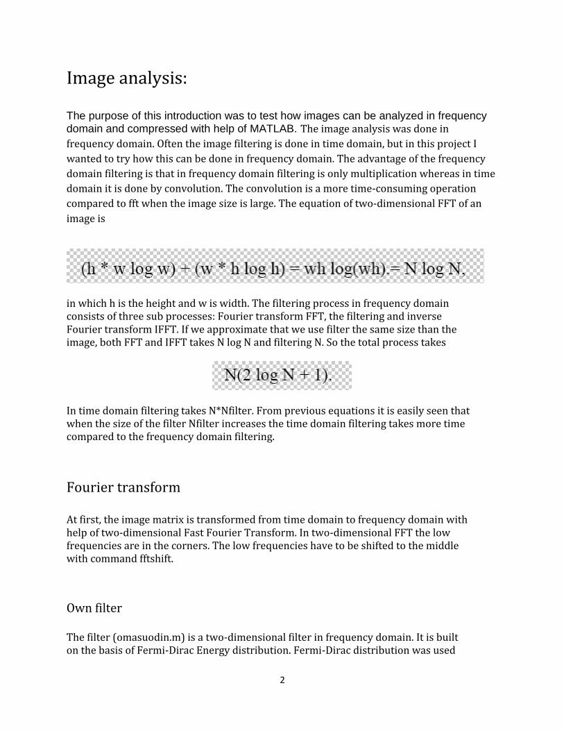
The filter “omasuodin” takes four parameters: the length and the height of the filter, the cut-off frequency and the sternness factor. In the figures 1 and 2 are shown to example of the filter “omasuodin”. Figure 1 shows a lowpass filter, whose cut-off frequency is 30 and steepness factor is 5. In figure 2 is a highpass filter with the same specification.

Figure 1 Lowpass filter (fc=30, steepness = 5)

4

Figure 2 Highpass filter (fc=30, steepness=5)

Smoothing In this project smoothing was done by multiplying the FFT of the image with a lowpass filter. Lowpass filtering smoothes the image because it suppresses the rapidly changing brightness values (high frequencies) from the original image. The amount of the suppression is determined by the cut-off frequency of the filter. If the steepness of the filter is too high (filter near ideal), filter leaves undesirable artifacts in image. Artifacts are seen as ripples or waves near the boundaries in the image. In figure 3, an example of image smoothing is seen. In this case the filter’s cutoff frequency was 30 and the steepness factor was 2. The suppression of high frequencies is clearly seen in the lowpass filtered FFT of the image

5

Figure 3 Smoothing of the image

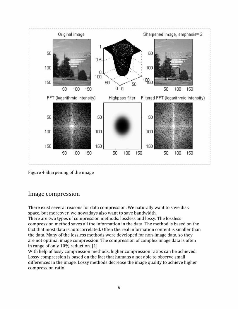
Sharpening The sharpening is done by first highpass filtering the FFT of the image and the adding the highpassed image to original image. The highpass filter finds the edges of the image, because it passes only the high-frequency information. High frequencies correspond to the rapidly changing gray levels, edges. As with lowpass filter, too steep a filter (near ideal) causes artifacts. The highpassed image (edges) are multiplied by an emphasis factor and added to the original image. The emphasis factor determines how much the image is sharpened. If the emphasis factor is high, overflow may happen. Overflow is seen as noise (black and white points) in the image. This effect is avoided by rescaling the image after filtering so that values over the maximum (255) are set to maximum and values under the minimum (0) are set to minimum. In the figure 4, an example of sharpening of the image is seen. In this case the cut-off frequency of the highpass filter was 30 and the steepness factor 5. The edge emphasis factor was 2.

6

Figure 4 Sharpening of the image

Image compression There exist several reasons for data compression. We naturally want to save disk space, but moreover, we nowadays also want to save bandwidth. There are two types of compression methods: lossless and lossy. The lossless compression method saves all the information in the data. The method is based on the fact that most data is autocorrelated. Often the real information content is smaller than the data. Many of the lossless methods were developed for non-image data, so they are not optimal image compression. The compression of complex image data is often in range of only 10% reduction. [1] With help of lossy compression methods, higher compression ratios can be achieved. Lossy compression is based on the fact that humans a not able to observe small differences in the image. Lossy methods decrease the image quality to achieve higher compression ratio.

7

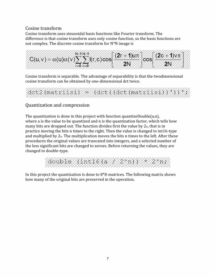
Cosine transform Cosine transform uses sinusoidal basis functions like Fourier transform. The difference is that cosine transform uses only cosine function, so the basis functions are not complex. The discrete cosine transform for N*N image is

Cosine transform is separable. The advantage of separability is that the twodimensional cosine transform can be obtained by one-dimensional dct twice.

Quantization and compression The quantization is done in this project with function quantizeDouble(a,n), where a is the value to be quantized and n is the quantization factor, which tells how many bits are dropped out. The function divides first the value by 2n, that is in practice moving the bits n times to the right. Then the value is changed to int16-type and multiplied by 2n. The multiplication moves the bits n times to the left. After these procedures the original values are truncated into integers, and a selected number of the less significant bits are changed to zeroes. Before returning the values, they are changed to double-type.

In this project the quantization is done to 8*8-matrices. The following matrix shows how many of the original bits are preserved in the operation.

8

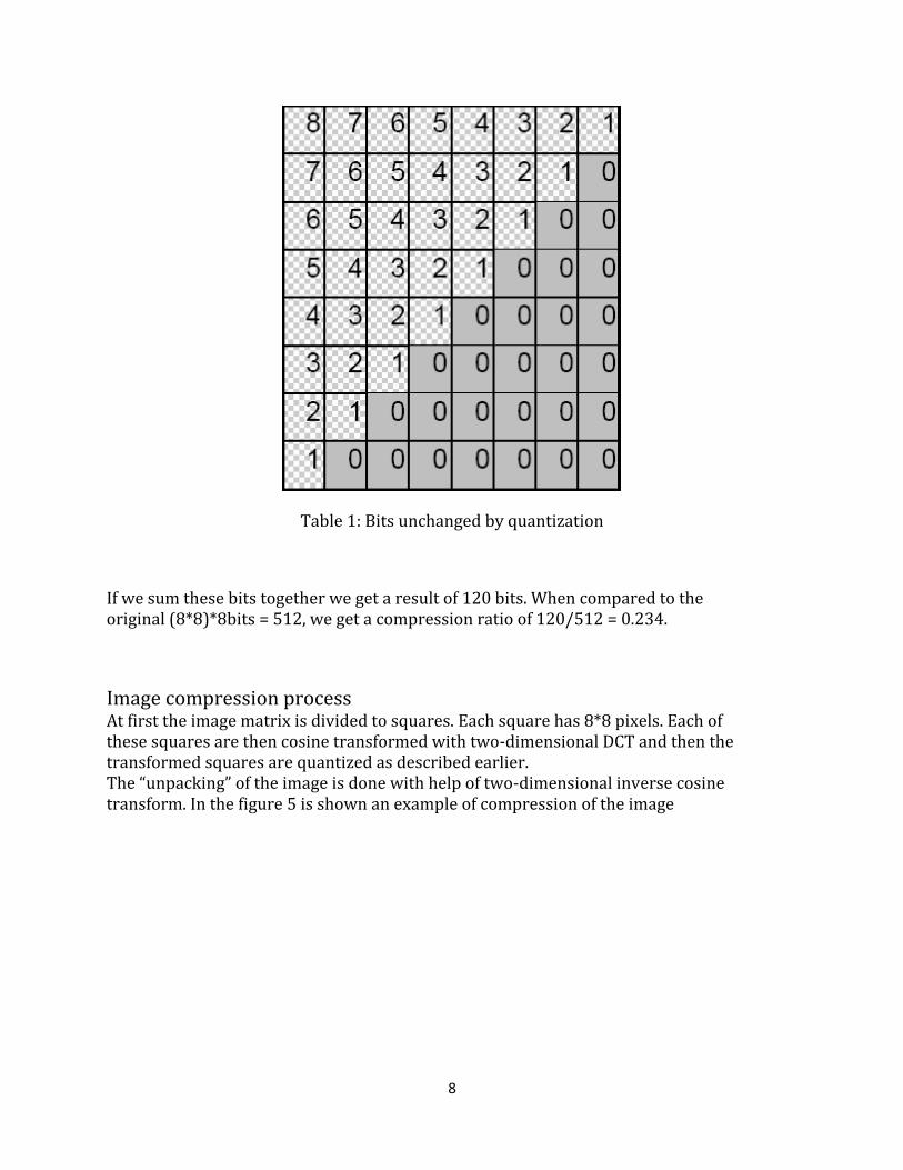
Table 1: Bits unchanged by quantization

If we sum these bits together we get a result of 120 bits. When compared to the original (8*8)*8bits = 512, we get a compression ratio of 120/512 = 0.234.

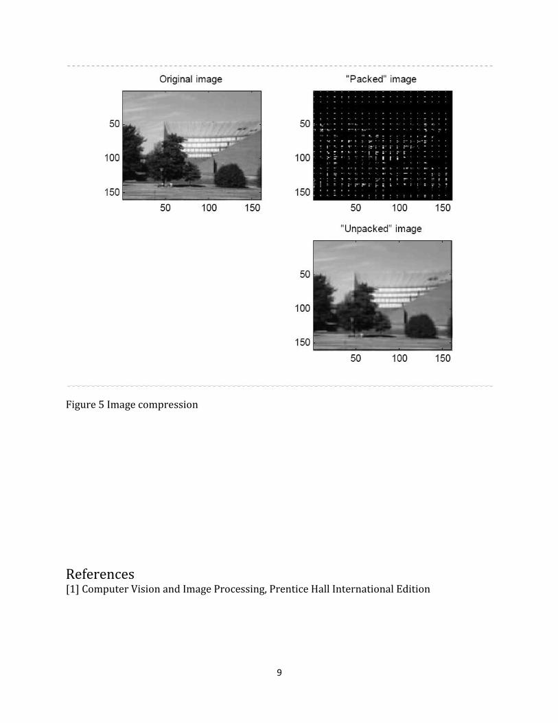
Image compression process At first the image matrix is divided to squares. Each square has 8*8 pixels. Each of these squares are then cosine transformed with two-dimensional DCT and then the transformed squares are quantized as described earlier. The “unpacking” of the image is done with help of two-dimensional inverse cosine transform. In the figure 5 is shown an example of compression of the image

9

Figure 5 Image compression

References [1] Computer Vision and Image Processing, Prentice Hall International Edition

10

CHAPTER(2)

How to Compress We exploit the redundancy in digital audio, image, and video data and properties of human perception to remove unwanted pixels. Also, as Digital audio is a series of sample values; image is a rectangular array of pixel values; video is a sequence of images played out at a certain rate neighboring sample values are correlated. In digital image, neighboring samples on a scanning line are normally similar (spatial

redundancy*). Human eye is less sensitive to the higher spatial frequency components than

the lower frequencies (transform coding).

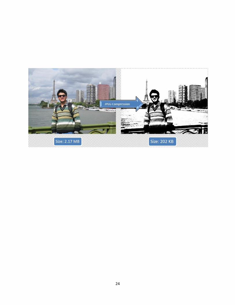
JPEG The name "JPEG" stands for Joint Photographic Experts Group. JPEG is a method of lossy compression for digitized photographic images. JPEG can achieve 10 to 1 compression with little perceptible loss in image quality. It works with colour and greyscale images and finds applications in satellite, medical etc. JPEG Encoding consists of following stages. The Major Steps in JPEG Coding involve: Image/Block Preparation DCT (Discrete Cosine Transformation) Quantization Entropy Coding o Zigzag Scan (Vectoring) o Differential Pulse Code Modulation (DPCM) on DC component o Run Length Encode (RLE) on AC components

11

Image/Block Preparation

Source image as 2-D matrix of pixel values

R, G, B format requires three matrices, one each for R, G, B quantized values

In Y, U, V representation, the U and V matrices can be half as small as the Y matrix

Source image matrix is divided into blocks of 8X8 submatrices

Smaller block size of 8x8 helps DCT computation and individual blocks are sequentially fed to the ___DCT which transforms each block separately

Why 8x8 is the block size? It is a tradeoff between compression, image quality and complexity. Smaller blocks are

simpler to implement but less scope for compression. Larger blocks are more complicated

but there are more frequency coefficients

12

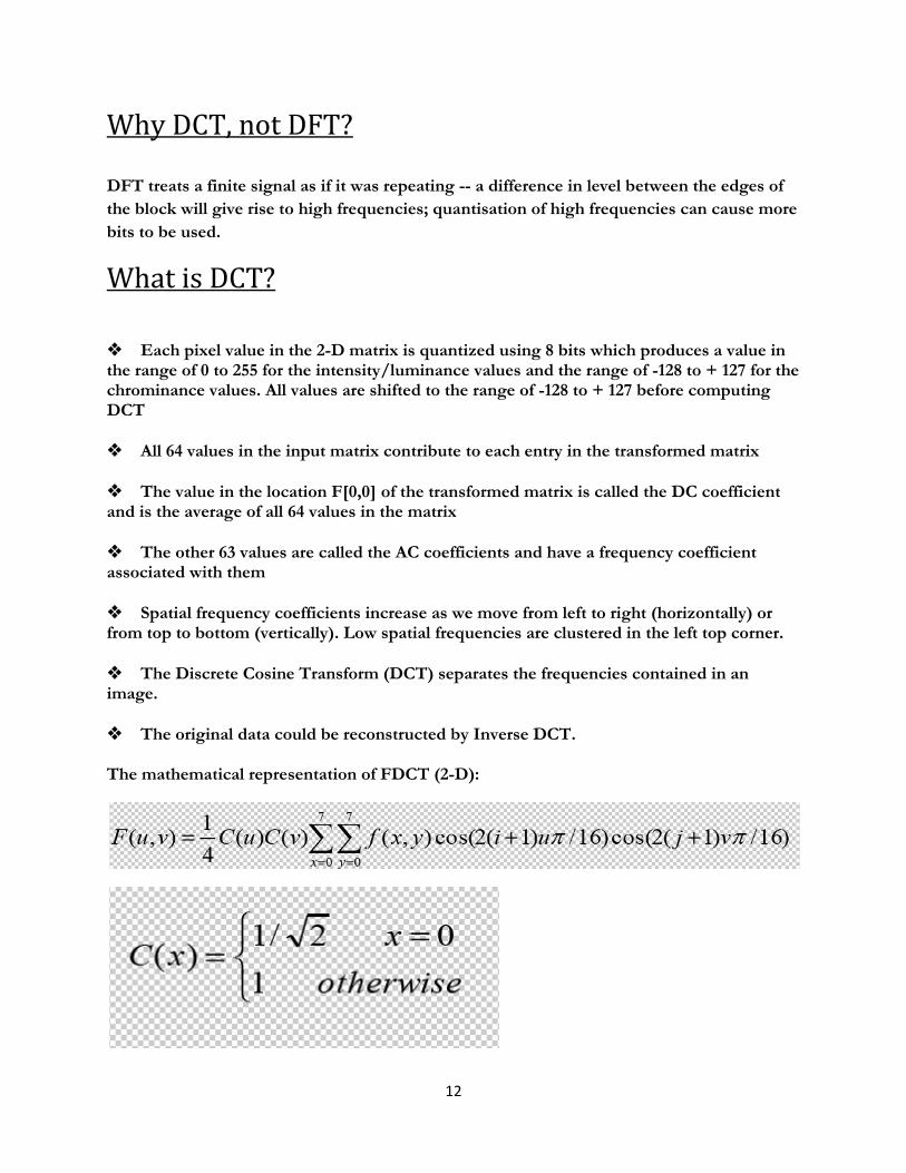
Why DCT, not DFT? DFT treats a finite signal as if it was repeating -- a difference in level between the edges of

the block will give rise to high frequencies; quantisation of high frequencies can cause more

bits to be used.

What is DCT?

Each pixel value in the 2-D matrix is quantized using 8 bits which produces a value in the range of 0 to 255 for the intensity/luminance values and the range of -128 to + 127 for the chrominance values. All values are shifted to the range of -128 to + 127 before computing DCT

All 64 values in the input matrix contribute to each entry in the transformed matrix

The value in the location F[0,0] of the transformed matrix is called the DC coefficient and is the average of all 64 values in the matrix

The other 63 values are called the AC coefficients and have a frequency coefficient associated with them

Spatial frequency coefficients increase as we move from left to right (horizontally) or from top to bottom (vertically). Low spatial frequencies are clustered in the left top corner.

The Discrete Cosine Transform (DCT) separates the frequencies contained in an image.

The original data could be reconstructed by Inverse DCT. The mathematical representation of FDCT (2-D):

13

Quantization

The human eye responds to the DC coefficient and the lower spatial frequency coefficients

If the magnitude of a higher frequency coefficient is below a certain threshold, the eye will not detect it

Set the frequency coefficients in the transformed matrix whose amplitudes are less than a defined threshold to zero (these coefficients cannot be recovered during decoding)

During quantization, the size of the DC and AC coefficients are reduced

A division operation is performed using the predefined threshold value as the divisor

Quantization Table

Threshold values vary for each of the 64 DCT coefficients and are held in a 2-D matrix

Trade off between the level of compression required and the information loss that is acceptable

JPEG standard includes two default quantization tables -- one for the luminance coefficients and the other for use with the two sets of chrominance coefficients. Customized tables may be used

14

Entropy Coding Vectoring -- 2-D matrix of quantized DCT coefficients are represented in the form of a single-dimensional vector

After quantization, most of the high frequency coefficients (lower right corner) are zero.

To exploit the number of zeros, a zig-zag scan of the matrix is used

Zig-zag scan allows all the DC coefficients and lower frequency AC coefficients to be scanned first

DC coefficients are encoded using differential encoding and AC coefficients are encoded using run-length encoding. Huffman coding is used to encode both after that.

Differential Encoding DC coefficient is the largest in the transformed matrix.

DC coefficient varies slowly from one block to the next.

Only the difference in value of the DC coefficients is encoded. Number of bits required to encode is reduced.

The difference values are encoded in the form (SSS, value) where SSS field indicates the number of bits needed to encode the value and the value field indicates the binary form.

Run-length Encoding 63 values of the AC coefficients

Long strings of zeros because of the zig-zag scan

Each AC coefficient encoded as a pair of values -- (skip, value), skip indicates the number of zeros in the run and value is the next non-zero coefficient

15

Huffman Encoding Long strings of binary digits replaced by shorter codewords

Prefix property of the huffman codewords enable decoding the encoded bitstream unambiguously

Frame Building Encapsulates the information relating to an encoded image

16

17

18

19

20

21

22

23

RESULT:

24

25

26

Results:

27

28

Chapter (3)

Method

in my project I used lossy compression with Block Truncation Code (BTC)

Image file formats

A digital image is a representation of a two-dimensional image as a finite set of

digital values, called pixels. Typically, the pixels are stored in computer memory as a

two-dimensional array of small integers and these values are transmitted or stored

in a compressed form. Digital images are very large in uncompressed form.

Compression techniques are used to reduce image file size for storage, processing,

and transmission. Compression is a reversible conversion of data to a format that

requires fewer bits, usually performed so that the data can be stored or transmitted

more efficiently . In effect, the objective is to reduce redundancy of the image data in

order to be able to store or transmit data in an efficient form. It can be lossy or

lossless. Lossless compression is sometimes preferred for artificial images such as

technical drawings, icons or comics. This is because lossy compression methods,

especially when used at low bit rates, can introduce compression artifacts. Lossless

compression methods may also be preferred for high value content, such as medical

imagery or image scans made for archival purposes.

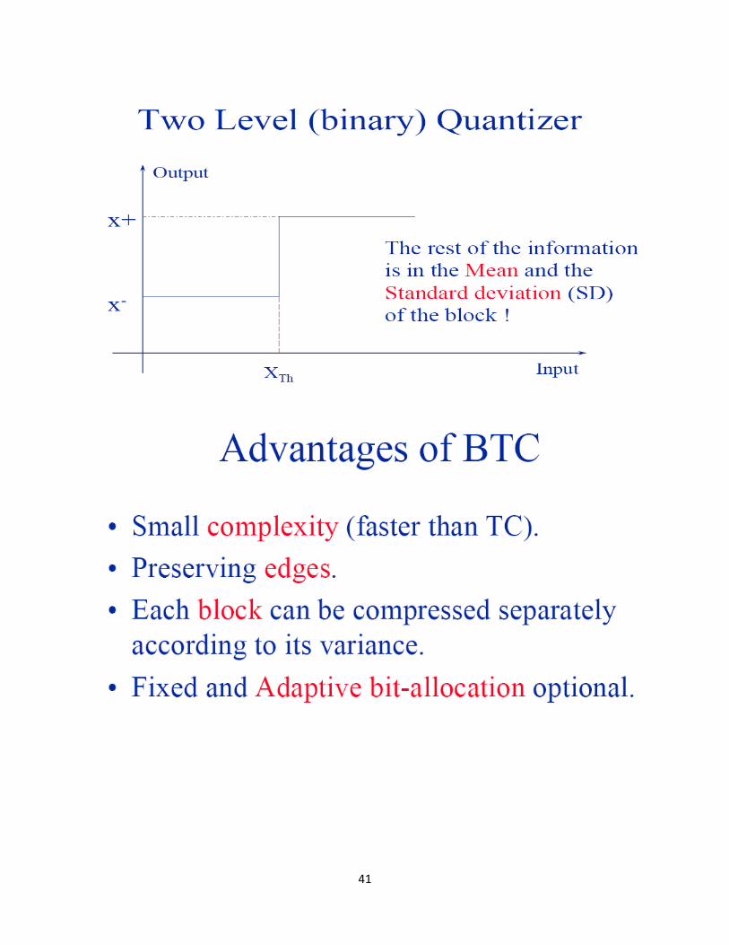
Block Truncation Coding :

Block Truncation Coding, or BTC, is a type of lossy image compression technique for

greyscale images. It divides the original images into blocks and then uses a quantizer

to reduce the number of grey levels in each block whilst maintaining the same mean

and standard deviation. It is an early predecessor of the popular hardware DXTC

technique, although BTC compression method was first adapted to colour long

before DXTC using a very similar approach called Colour Cell Compression BTC has

also been adapted to video compression .

http://en.wikipedia.org/wiki/Lossy_compression

http://en.wikipedia.org/wiki/Greyscale

http://en.wikipedia.org/w/index.php?title=Grey_levels&action=edit&redlink=1

http://en.wikipedia.org/wiki/Mean

http://en.wikipedia.org/wiki/Standard_deviation

http://en.wikipedia.org/wiki/DXTC

29

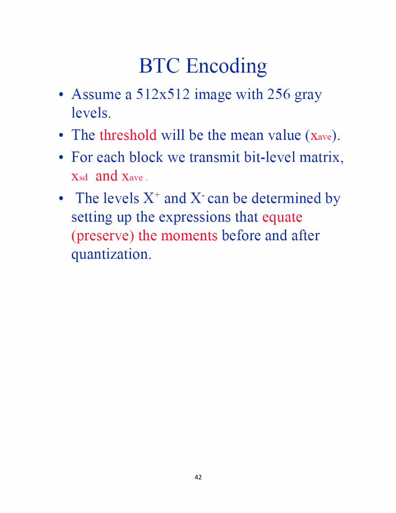
Compression procedure :

A 256x256 pixel image is divided into blocks of typically 4x4 pixels. For each block

the Mean and Standard Deviation are calculated, these values change from block to

block. These two values define what values the reconstructed or new block will have,

in other words the blocks of the BTC compressed image will all have the same mean

and standard deviation of the original image. A two level quantization on the block is

where we gain the compression, it is performed as follows:

Where x(i,j) are pixel elements of the original block and y(i,j) are elements of the

compressed block. In words this can be explained as: If a pixel value is greater than

the mean it is assigned the value "1", otherwise "0". Values equal to the mean can

have either a "1" or a "0" depending on the preference of the person or organisation

implementing the algorithm.

This 16 bit block is stored or transmitted along with the values of Mean and Standard

Deviation. Reconstruction is made with two values "a" and "b" which preserve the

mean and the standard deviation. The values of "a" and "b" can be computed as

follows:

Where σ is the standard deviation, m is the total number of pixels in the block and q

is the number of pixels greater than the mean ( )

To reconstruct the image, or create its approximation, elements assigned a 0 are

replaced with the "a" value and elements assigned a 1 are replaced with the "b"

http://en.wikipedia.org/wiki/Pixel

30

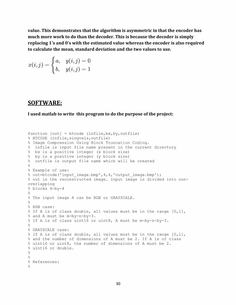
value. This demonstrates that the algorithm is asymmetric in that the encoder has

much more work to do than the decoder. This is because the decoder is simply

replacing 1's and 0's with the estimated value whereas the encoder is also required

to calculate the mean, standard deviation and the two values to use.

SOFTWARE:

I used matlab to write this program to do the purpose of the project:

function [out] = btcode (infile,bx,by,outfile)

% BTCODE (infile,singvals,outfile)

% Image Compression Using Block Truncation Coding.

% infile is input file name present in the current directory

% bx is a positive integer (x block size)

% by is a positive integer (y block size)

% outfile is output file name which will be created

%

% Example of use:

% out=btcode('input_image.bmp',4,4,'output_image.bmp');

% out is the reconstructed image. Input image is divided into non-

overlapping

% blocks 4-by-4

%

% The input image A can be RGB or GRAYSCALE.

%

% RGB case:

% If A is of class double, all values must be in the range [0,1],

% and A must be m-by-n-by-3.

% If A is of class uint16 or uint8, A must be m-by-n-by-3.

%

% GRAYSCALE case:

% If A is of class double, all values must be in the range [0,1],

% and the number of dimensions of A must be 2. If A is of class

% uint16 or uint8, the number of dimensions of A must be 2.

% uint16 or double.

%

%

% References:

%

31

% For more details concernings the algorithm implemented please visit the

following link:

%

%

http://www.ee.latrobe.edu.au/~dennis/teaching/ELE42IPC/ELE42IPC_imgpro/nod

e14.html

%

%

% Please contribute if you find this software useful.

% Report bugs to [email protected]

%

%

%*****************************************************************

% Luigi Rosa

% Via Centrale 27

% 67042 Civita di Bagno

% L'Aquila --- ITALY

% email [email protected]

% mobile +39 340 3463208

% http://utenti.lycos.it/matlab

%*****************************************************************

%

%

if (exist(infile)==2)

a = imread(infile);

figure('Name','Input image');

imshow(a);

else

warndlg('The file does not exist.',' Warning ');

out=[];

return

end

%------------------------------------------------------

if isgray(a)

dvalue = double(a);

dx=size(dvalue,1);

dy=size(dvalue,2);

% if input image size is not a multiple of block size image is resized

modx=mod(dx,bx);

mody=mod(dy,by);

dvalue=dvalue(1:dx-modx,1:dy-mody);

% the new input image dimensions (pixels)

dx=dx-modx;

dy=dy-mody;

% number of non overlapping blocks required to cover

% the entire input image

nbx=size(dvalue,1)/bx;

nby=size(dvalue,2)/by;

% the output compressed image

matrice=zeros(bx,by);

32

% the compressed data

m_u=zeros(nbx,nby);

m_l=zeros(nbx,nby);

mat_log=logical(zeros(bx,by));

posbx=1;

for ii=1:bx:dx

posby=1;

for jj=1:by:dy

% the current block

blocco=dvalue(ii:ii+bx-1,jj:jj+by-1);

% the average gray level of the current block

m=mean(mean(blocco));

% the logical matrix correspoending to the current block

blocco_binario=(blocco>=m);

% the number of pixel (of the current block) whose gray level

% is greater than the average gray level of the current block

K=sum(sum(double(blocco_binario)));

% the average gray level of pixels whose level is GREATER than

% the block average gray level

mu=sum(sum(double(blocco_binario).*blocco))/K;

% the average gray level of pixels whose level is SMALLER than


if K==bx*by

ml=0;

else

ml=sum(sum(double(~blocco_binario).*blocco))/(bx*by-K);

end

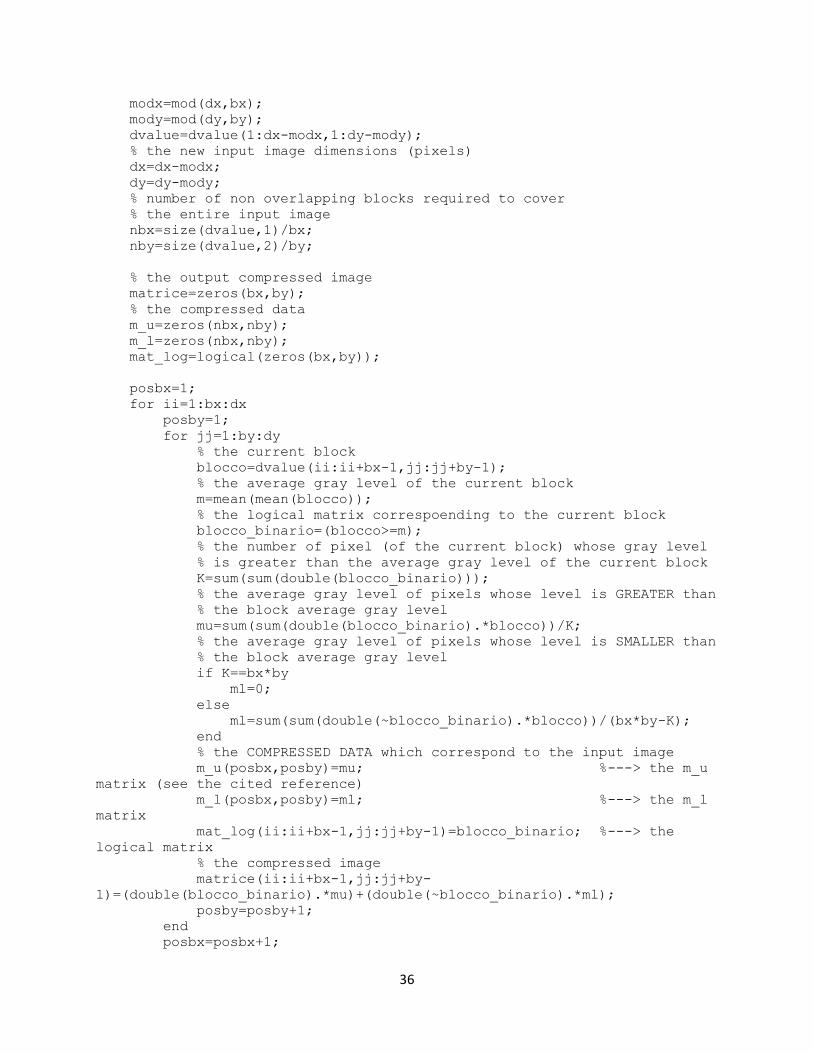
% the COMPRESSED DATA which correspond to the input image

m_u(posbx,posby)=mu; %---> the m_u

matrix (see the cited reference)

m_l(posbx,posby)=ml; %---> the m_l

matrix

mat_log(ii:ii+bx-1,jj:jj+by-1)=blocco_binario; %---> the

logical matrix

% the compressed image

matrice(ii:ii+bx-1,jj:jj+by-

1)=(double(blocco_binario).*mu)+(double(~blocco_binario).*ml);

posby=posby+1;

end

posbx=posbx+1;

end

% display the logical matrix

figure('Name','Logical matrix');

imshow(mat_log);

if isa(a,'uint8')

out=uint8(matrice);

figure('Name','Compressed image');

imshow(out);

imwrite(out, outfile);

return

33

end

if isa(a,'uint16')

out=uint16(matrice);


imshow(out);


return

end

if isa(a,'double')

out=(matrice);


imshow(out);


return

end

end

%------------------------------------------------------

if isrgb(a)

double_a=double(a);

ax=size(a,1)-mod(size(a,1),bx);

ay=size(a,2)-mod(size(a,2),by);

out_rgb=zeros(ax,ay,3);

%-----------------------------------------------------------

%-----------------------------------------------------------

% ----------------------- RED component ------------------

dvalue=double_a(:,:,1);

dx=size(dvalue,1);

dy=size(dvalue,2);


modx=mod(dx,bx);

mody=mod(dy,by);



dx=dx-modx;

dy=dy-mody;








m_u=zeros(nbx,nby);

m_l=zeros(nbx,nby);


34

posbx=1;

for ii=1:bx:dx

posby=1;

for jj=1:by:dy

% the current block














if K==bx*by

ml=0;

else


end





matrix


logical matrix




posby=posby+1;

end

posbx=posbx+1;

end

out_rgb(:,:,1)=matrice;

% ----------------------- GREEN component ------------------


dx=size(dvalue,1);

dy=size(dvalue,2);


modx=mod(dx,bx);

mody=mod(dy,by);



dx=dx-modx;

dy=dy-mody;




35





m_u=zeros(nbx,nby);

m_l=zeros(nbx,nby);


posbx=1;

for ii=1:bx:dx

posby=1;

for jj=1:by:dy

% the current block














if K==bx*by

ml=0;

else


end





matrix


logical matrix




posby=posby+1;

end

posbx=posbx+1;

end


% ----------------------- BLUE component ------------------


dx=size(dvalue,1);

dy=size(dvalue,2);


36

modx=mod(dx,bx);

mody=mod(dy,by);



dx=dx-modx;

dy=dy-mody;








m_u=zeros(nbx,nby);

m_l=zeros(nbx,nby);


posbx=1;

for ii=1:bx:dx

posby=1;

for jj=1:by:dy

% the current block














if K==bx*by

ml=0;

else


end





matrix


logical matrix




posby=posby+1;

end

posbx=posbx+1;

37

end


%------------------------------------------ -----------------

%-----------------------------------------------------------

%-----------------------------------------------------------

if isa(a,'uint8')

out=uint8(out_rgb);


imshow(out);


return

end

if isa(a,'uint16')

out=uint16(out_rgb);


imshow(out);


return

end

if isa(a,'double')

out=(out_rgb);


imshow(out);


return

end

end

%-------------------------

38

Chapter(4)

RESULT:

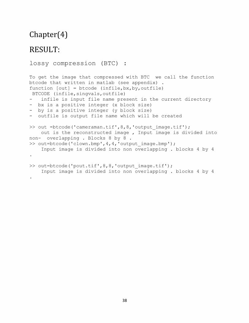
lossy compression (BTC) :

To get the image that compressed with BTC we call the function

btcode that written in matlab (see appendix) .

function [out] = btcode (infile,bx,by,outfile)

BTCODE (infile,singvals,outfile)

- infile is input file name present in the current directory

- bx is a positive integer (x block size)

- by is a positive integer (y block size)

- outfile is output file name which will be created

>> out =btcode('cameraman.tif',8,8,'output_image.tif');

out is the reconstructed image , Input image is divided into

non- overlapping . Blocks 8 by 8 .

>> out=btcode('clown.bmp',4,4,'output_image.bmp');

Input image is divided into non overlapping . blocks 4 by 4

.

>> out=btcode('pout.tif',8,8,'output_image.tif');

Input image is divided into non overlapping . blocks 4 by 4

.

39

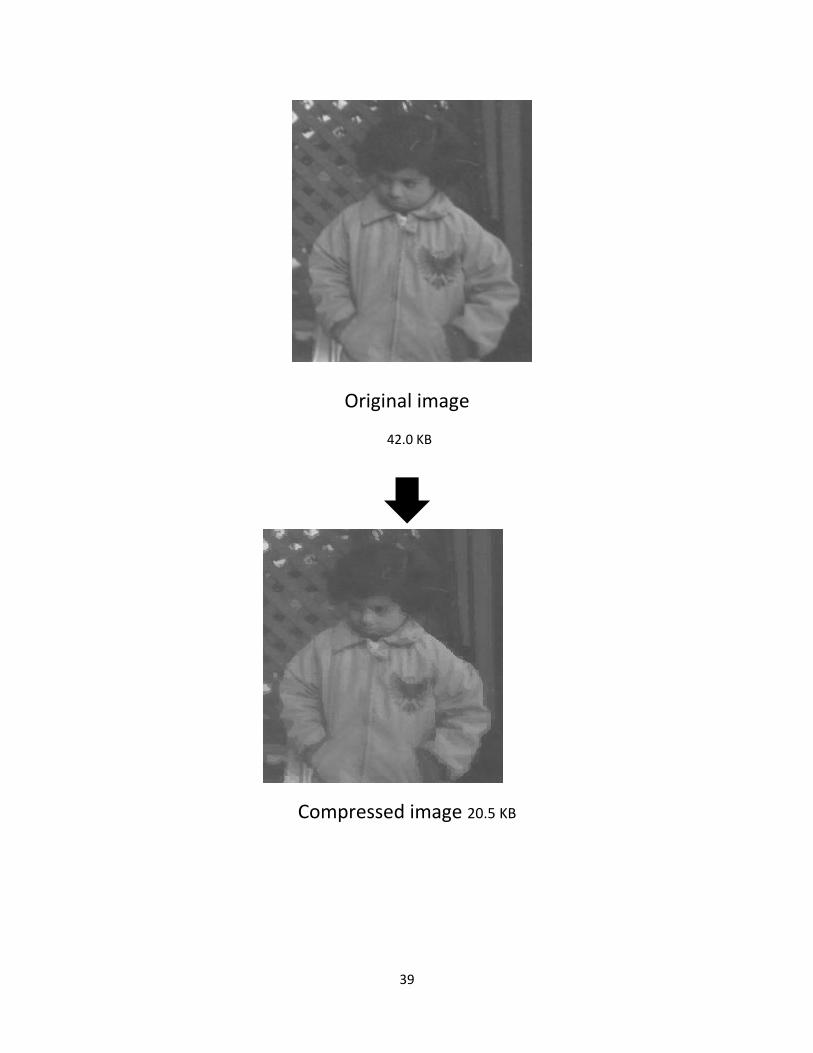
Original image

42.0 KB

Compressed image 20.5 KB

40

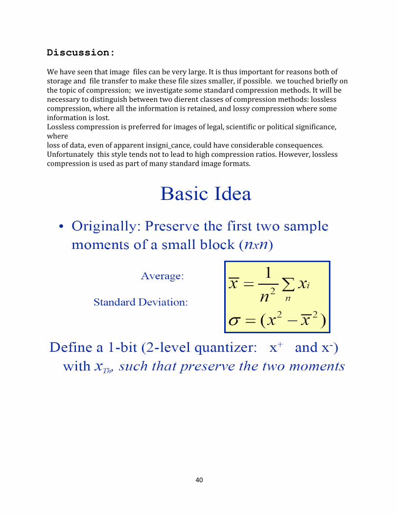
Discussion:

We have seen that image files can be very large. It is thus important for reasons both of storage and file transfer to make these file sizes smaller, if possible. we touched briefly on the topic of compression; we investigate some standard compression methods. It will be necessary to distinguish between two dierent classes of compression methods: lossless compression, where all the information is retained, and lossy compression where some information is lost. Lossless compression is preferred for images of legal, scientific or political significance, where loss of data, even of apparent insigni_cance, could have considerable consequences. Unfortunately this style tends not to lead to high compression ratios. However, lossless compression is used as part of many standard image formats.

41

42

43

44

45

46

47

Chapter (5)

Conclusion

Future Works

This project could be extended or utilised in a great

number of areas. As a simple image capture and display

device, image quality could firstly be increased by

using a greyscale display. This would remove the need

for the compression process, allowing true greyscale

images to be displayed and also greatly speeding up the

process of capture and display. A higher resolution

display would also improve image quality. A colour

display could also be used, although this would require

a large increase in the available memory space. Due to

the light weight and potentially extremely small size

of the device, future development could include

portable or wearable applications.

Also , there are a number of techniques being developed

claiming to improve the image compression that used in

matlab and this techniques Improve image quality and

processing speed ,

As an image capture system, the interface between an

image sensor and microcontroller could have many

additional applications, for example machine vision

where a display may not be required. This could be

implemented simply by extending the software. Again,

the lightweight and potentially small size of the

device would make it well suited to portable

applications in areas such as robotics.

48

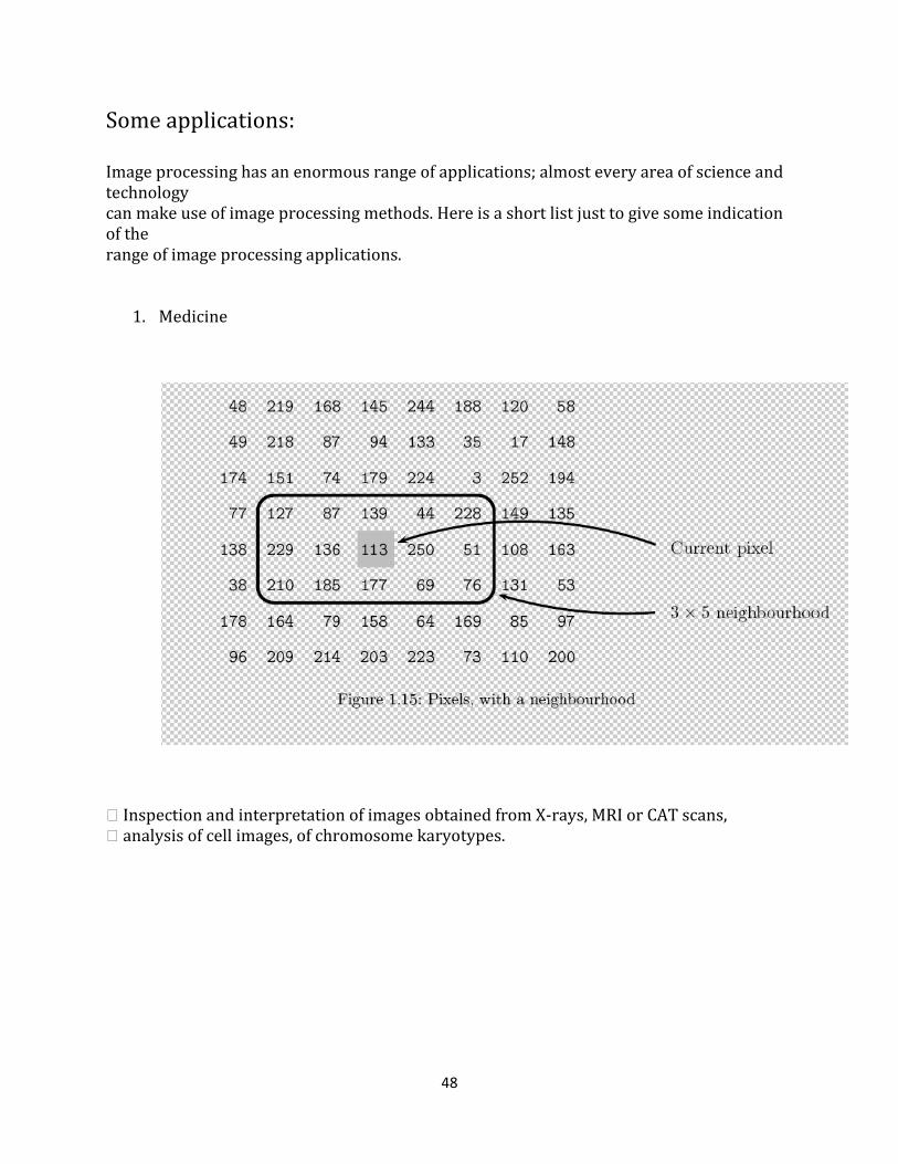
Some applications: Image processing has an enormous range of applications; almost every area of science and technology can make use of image processing methods. Here is a short list just to give some indication of the range of image processing applications.

1. Medicine

� Inspection and interpretation of images obtained from X-rays, MRI or CAT scans, � analysis of cell images, of chromosome karyotypes.

49

Refernces

Image Data Compression By MOHAMMED MUSA ...

Documents