Image Compression - Vis Centerryang/Teaching/cs635-2016spring/Lectures/11...Image Compression Lossy Compression and JPEG ... Discrete Cosine Transform ... Code for generating the Quantization

1

Image Compression

Lossy Compressionand JPEG

Review

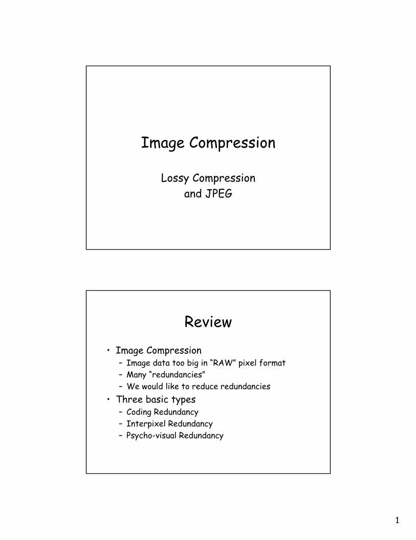
• Image Compression– Image data too big in “RAW” pixel format– Many “redundancies”– We would like to reduce redundancies

• Three basic types– Coding Redundancy– Interpixel Redundancy– Psycho-visual Redundancy

2

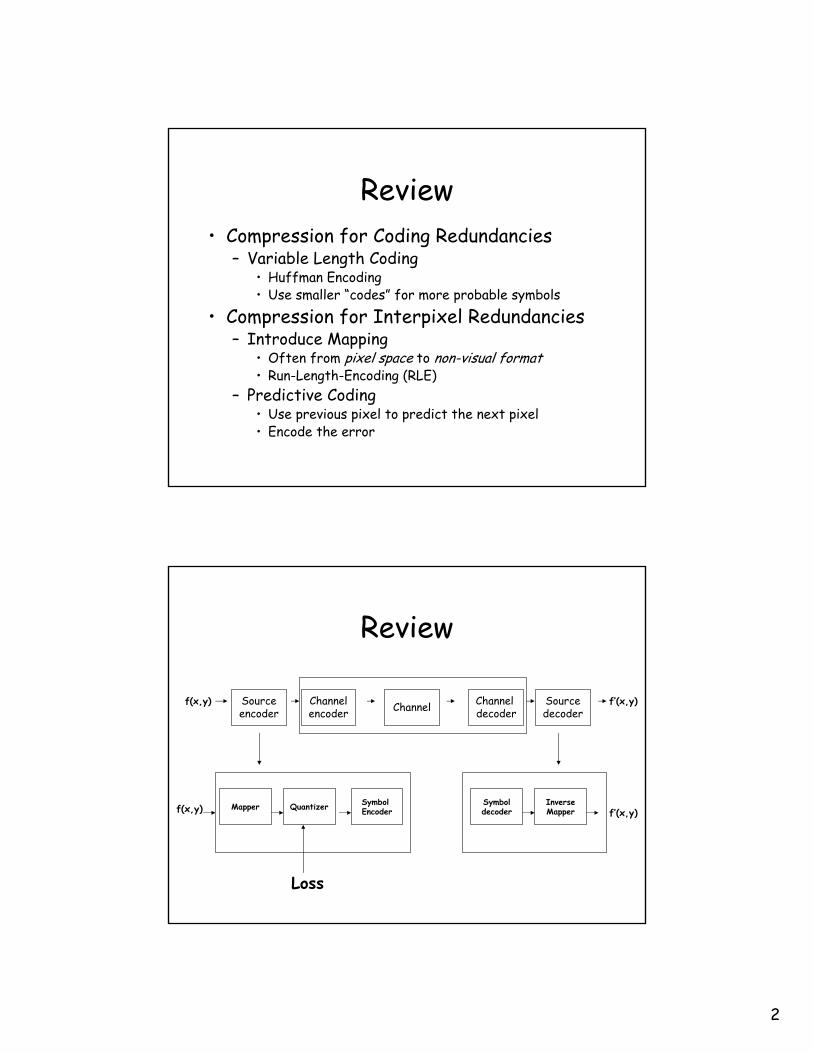
Review• Compression for Coding Redundancies

– Variable Length Coding• Huffman Encoding• Use smaller “codes” for more probable symbols

• Compression for Interpixel Redundancies– Introduce Mapping

• Often from pixel space to non-visual format• Run-Length-Encoding (RLE)

– Predictive Coding• Use previous pixel to predict the next pixel• Encode the error

Review

Sourceencoder

Channelencoder Channel Channel

decoderSourcedecoder

f(x,y) f’(x,y)

f’(x,y)Mapper Quantizer Symbol

EncoderSymboldecoder

InverseMapperf(x,y)

Loss

3

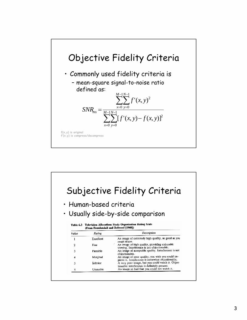
Objective Fidelity Criteria• Commonly used fidelity criteria is

– mean-square signal-to-noise ratio defined as:

∑∑

∑∑−

=

−

=

−

=

−

=

−= 1

0

1

0

2

1

0

1

0

2

)],(),('[

),('

M

x

N

y

M

x

N

yms

yxfyxf

yxfSNR

f(x,y) is originalf’(x,y) is compress/decompress

Subjective Fidelity Criteria• Human-based criteria• Usually side-by-side comparison

4

Lossy Compression• Compromise accuracy

– That is, we will allow for “error”– Distortion

• In exchange for increased compression– If the resulting distortion can be tolerated– Then we can gain substantial compression

• Exploit psycho-visual Redundancy– Our eye is less sensitive to high-frequencies– Can can “throw” away a lot of detail and image

looks the same

Lossy Compression

5

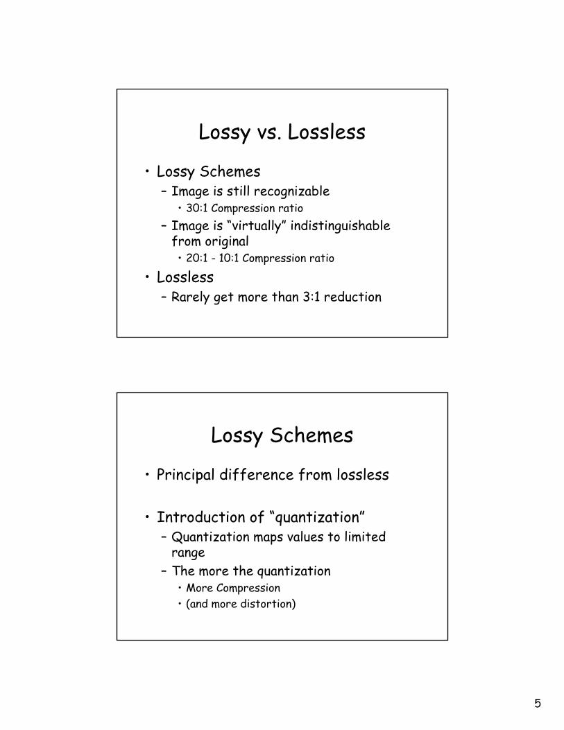
Lossy vs. Lossless

• Lossy Schemes– Image is still recognizable

• 30:1 Compression ratio– Image is “virtually” indistinguishable

from original• 20:1 - 10:1 Compression ratio

• Lossless– Rarely get more than 3:1 reduction

Lossy Schemes

• Principal difference from lossless

• Introduction of “quantization”– Quantization maps values to limited

range– The more the quantization

• More Compression• (and more distortion)

6

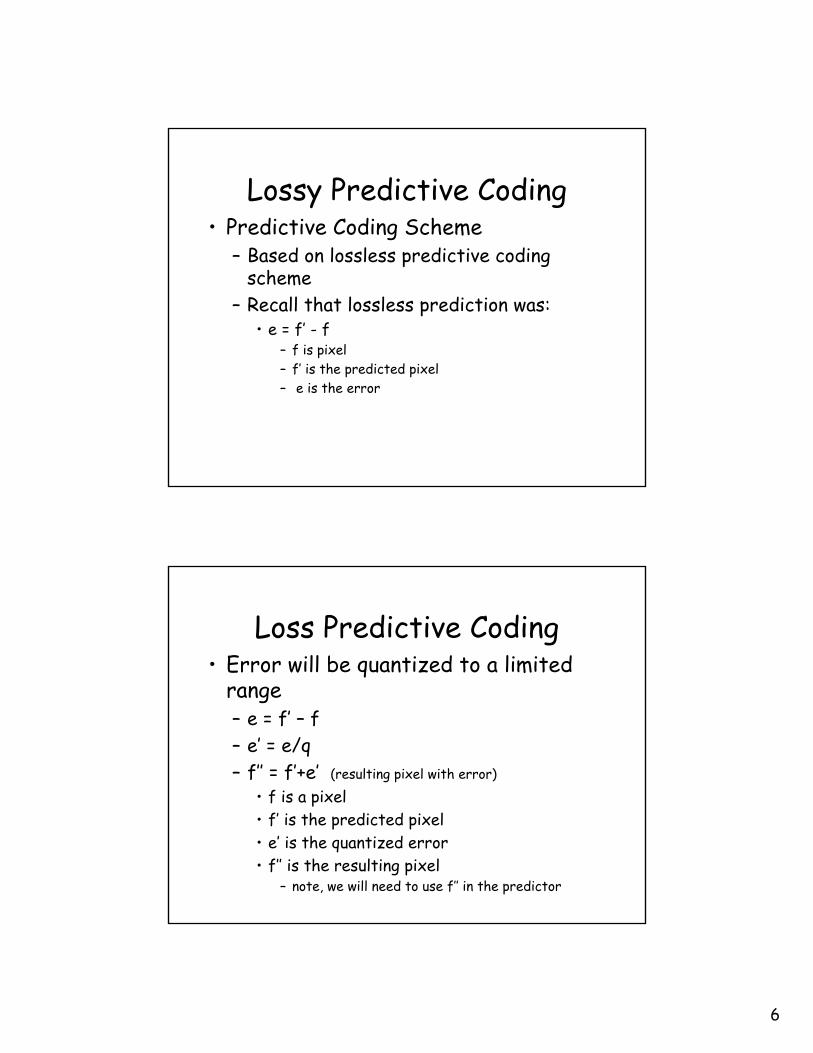
Lossy Predictive Coding• Predictive Coding Scheme

– Based on lossless predictive coding scheme

– Recall that lossless prediction was:• e = f’ - f

– f is pixel– f’ is the predicted pixel– e is the error

Loss Predictive Coding• Error will be quantized to a limited

range– e = f’ – f– e’ = e/q– f’’ = f’+e’ (resulting pixel with error)

• f is a pixel• f’ is the predicted pixel• e’ is the quantized error• f’’ is the resulting pixel

– note, we will need to use f’’ in the predictor

7

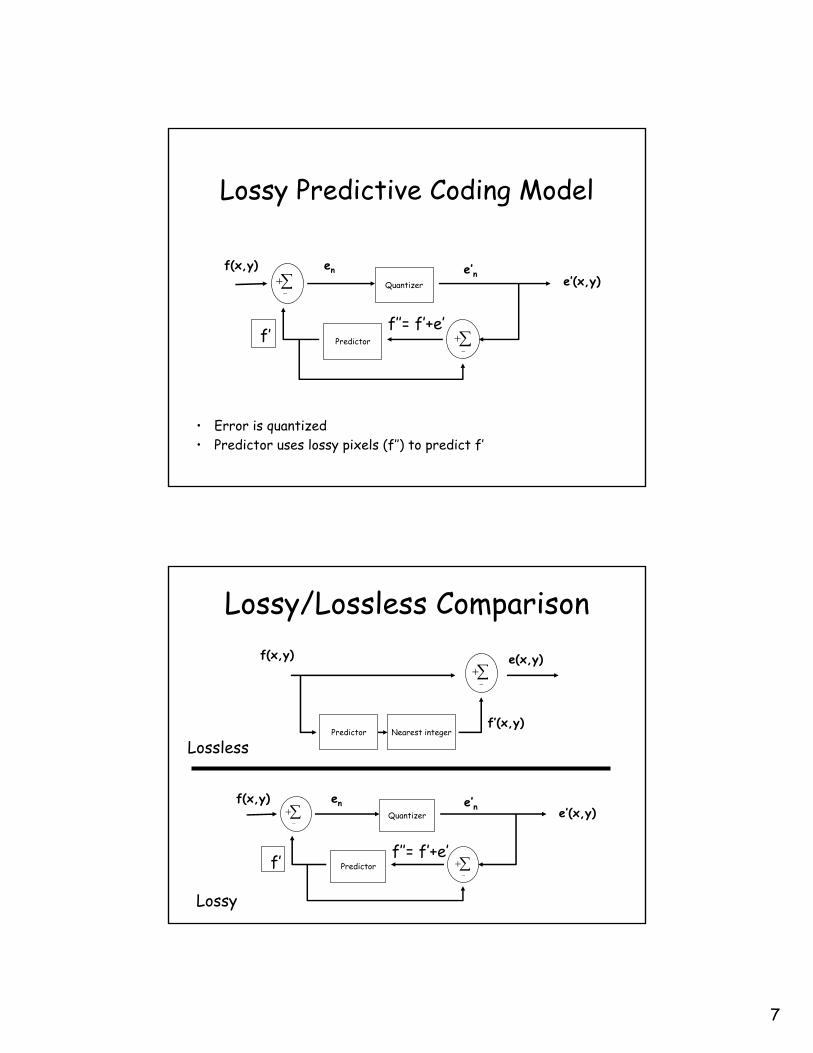
Lossy Predictive Coding Model

• Error is quantized• Predictor uses lossy pixels (f’’) to predict f’

Predictor

∑−

+f(x,y)

e’(x,y)en e’n

Quantizer

∑−

+f’f’’= f’+e’

Lossy/Lossless Comparison

Predictor Nearest integer

∑−

+f(x,y)

f’(x,y)

e(x,y)

Lossless

Lossy

Predictor

∑−

+f(x,y)

e’(x,y)en e’n

Quantizer

∑−

+f’ f’’= f’+e’

8

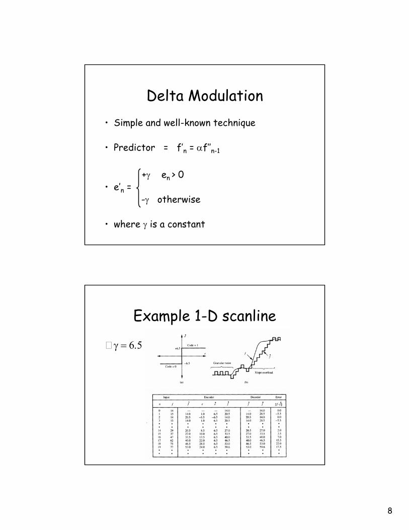
Delta Modulation• Simple and well-known technique

• Predictor = f’n = αf’’n-1

+γ en > 0• e’n =

-γ otherwise

• where γ is a constant

Example 1-D scanline

γ = 6.5

9

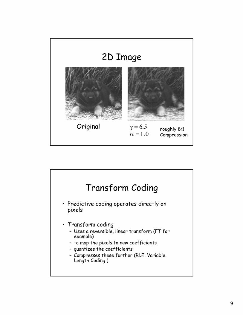
2D Image

γ = 6.5Originalα = 1.0

roughly 8:1Compression

Transform Coding• Predictive coding operates directly on

pixels

• Transform coding– Uses a reversible, linear transform (FT for

example)– to map the pixels to new coefficients– quantizes the coefficients– Compresses these further (RLE, Variable

Length Coding )

10

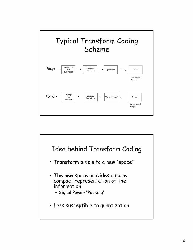
Typical Transform Coding Scheme

f(x,y) Constructnxn

subimages

ForwardTransform Quantizer

“De-quantizer”InverseTransform

Mergenxn

subimagesf’(x,y)

Other

Other

CompressedImage

CompressedImage

Idea behind Transform Coding

• Transform pixels to a new “space”

• The new space provides a more compact representation of the information– Signal Power “Packing”

• Less susceptible to quantization

11

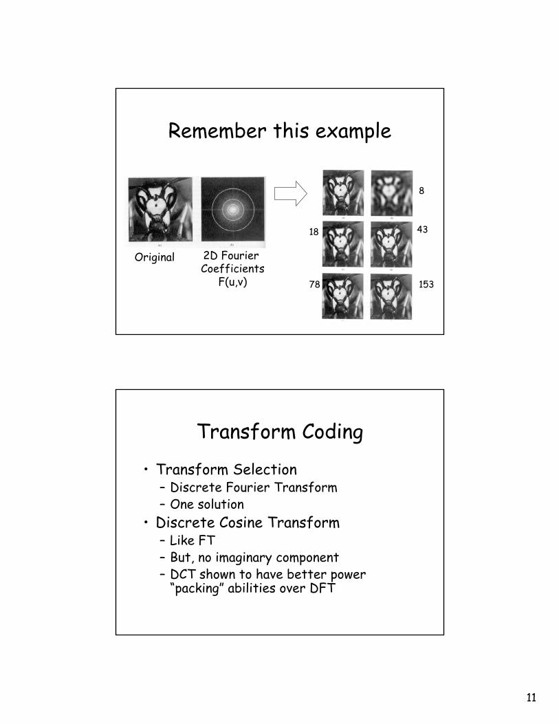
Remember this example

Original 2D Fourier Coefficients

F(u,v)

8

18 43

78 153

Transform Coding

• Transform Selection– Discrete Fourier Transform– One solution

• Discrete Cosine Transform– Like FT– But, no imaginary component– DCT shown to have better power

“packing” abilities over DFT

12

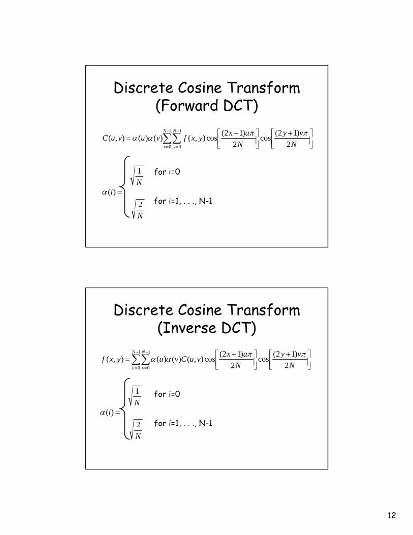
Discrete Cosine Transform(Forward DCT)

2

1

)(

2)12(cos

2)12(cos),()()(),(

1

0

1

0

N

Ni

Nvy

NuxyxfvuvuC

N

x

N

y

=

⎥⎦⎤

⎢⎣⎡ +

⎥⎦⎤

⎢⎣⎡ +

= ∑∑−

=

−

=

α

ππαα

for i=0

for i=1, . . ., N-1

Discrete Cosine Transform(Inverse DCT)

2

1

)(

2)12(cos

2)12(cos),()()(),(

1

0

1

0

N

Ni

Nvy

NuxvuCvuyxf

N

u

N

v

=

⎥⎦⎤

⎢⎣⎡ +

⎥⎦⎤

⎢⎣⎡ +

= ∑∑−

=

−

=

α

ππαα

for i=0

for i=1, . . ., N-1

13

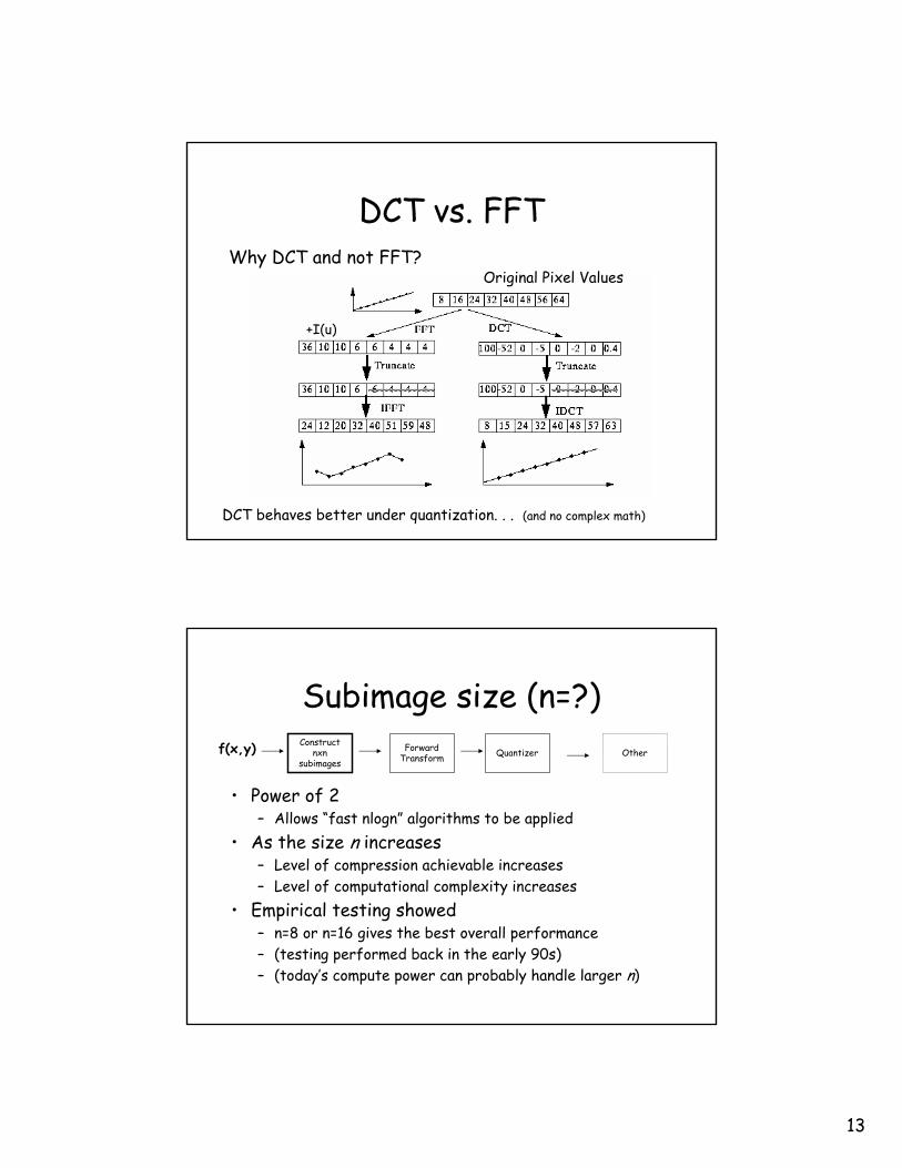
DCT vs. FFTWhy DCT and not FFT?

DCT behaves better under quantization. . . (and no complex math)

+I(u)

Original Pixel Values

Subimage size (n=?)

• Power of 2– Allows “fast nlogn” algorithms to be applied

• As the size n increases– Level of compression achievable increases– Level of computational complexity increases

• Empirical testing showed– n=8 or n=16 gives the best overall performance– (testing performed back in the early 90s)– (today’s compute power can probably handle larger n)

f(x,y) Constructnxn

subimages

ForwardTransform Quantizer Other

14

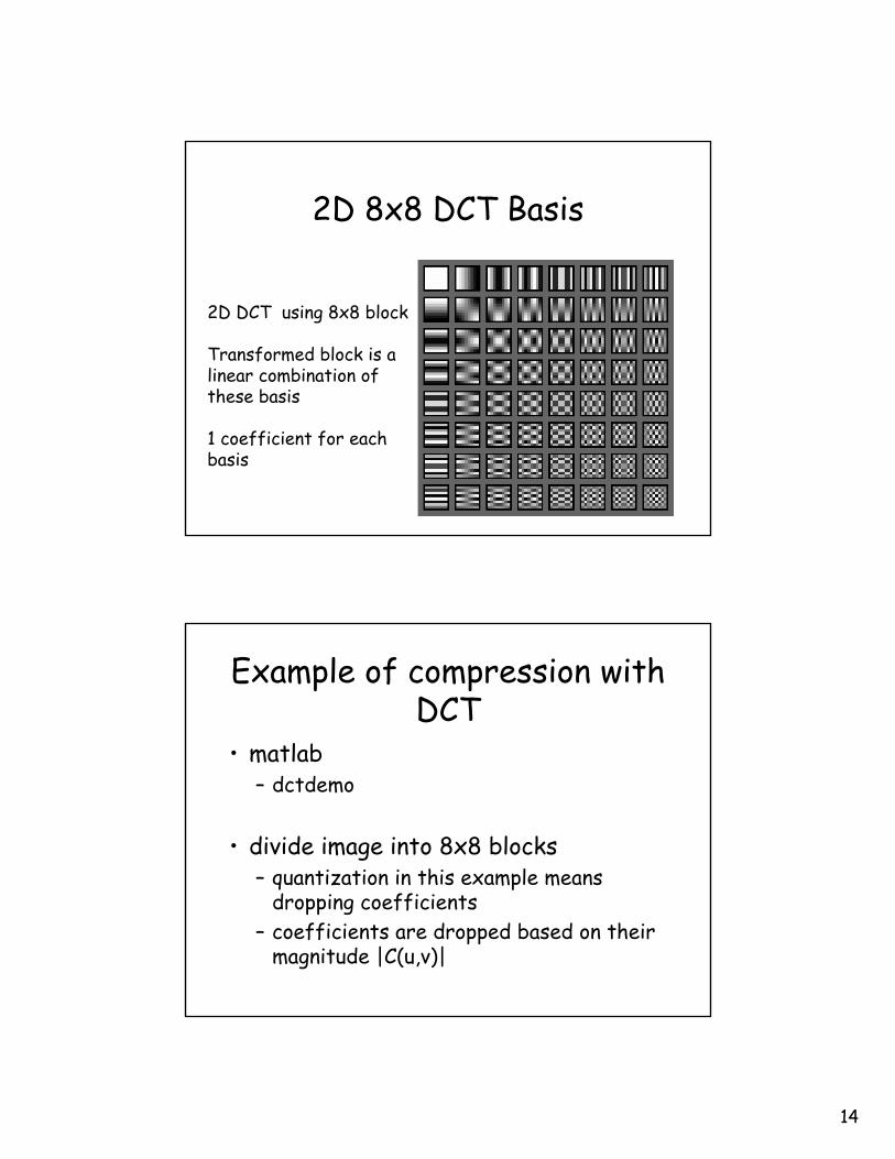
2D 8x8 DCT Basis

2D DCT using 8x8 block

Transformed block is a linear combination of these basis

1 coefficient for eachbasis

Example of compression with DCT

• matlab– dctdemo

• divide image into 8x8 blocks– quantization in this example means

dropping coefficients– coefficients are dropped based on their

magnitude |C(u,v)|

15

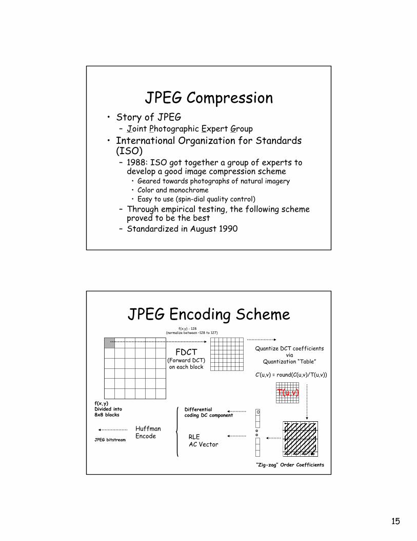
JPEG Compression• Story of JPEG

– Joint Photographic Expert Group• International Organization for Standards

(ISO)– 1988: ISO got together a group of experts to

develop a good image compression scheme• Geared towards photographs of natural imagery• Color and monochrome• Easy to use (spin-dial quality control)

– Through empirical testing, the following scheme proved to be the best

– Standardized in August 1990

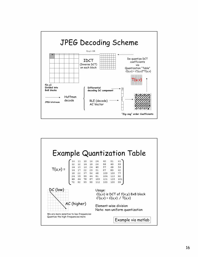
JPEG Encoding Scheme

f(x,y)Divided into8x8 blocks

FDCT(Forward DCT)on each block

Quantize DCT coefficientsvia

Quantization “Table”

C’(u,v) = round(C(u,v)/T(u,v))

“Zig-zag” Order Coefficients

RLEAC Vector

0Differentialcoding DC component

Huffman Encode

JPEG bitstream

T(u,v)

f(x,y) - 128(normalize between –128 to 127)

16

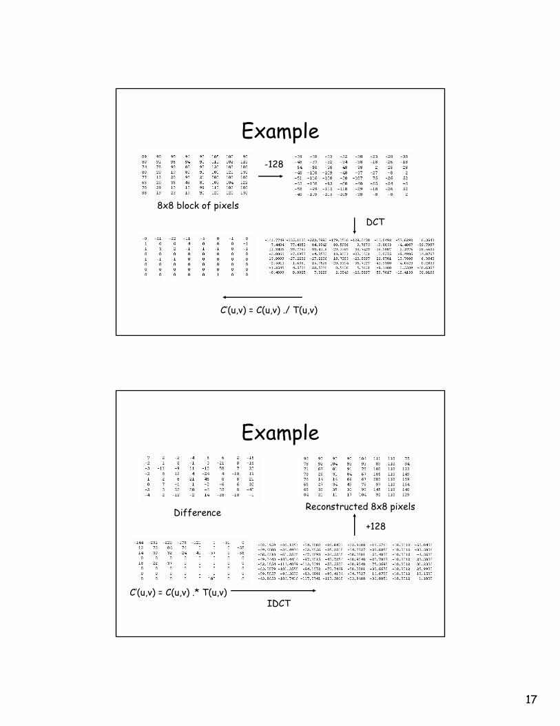
JPEG Decoding Scheme

f(x,y)Divided into8x8 blocks

IDCT(Inverse DCT)on each block

De-quantize DCT coefficients

via Quantization “Table”C(u,v) = C’(u,v)*T(u,v)

T(u,v)

“Zig-zag” order Coefficients

RLE (decode)AC Vector

0Differentialdecoding DC component

Huffman decode

JPEG bitstream

f(x,y) + 128

Example Quantization Table

Example via matlab

T(u,v) =

DC (low)

AC (higher)

We are more sensitive to low-frequenciesQuantize the high-frequencies more

Usage:C(u,v) is DCT of f(x,y) 8x8 blockC’(u,v) = C(u,v) ./ T(u,v)

Element-wise divisionNote: non-uniform quantization

17

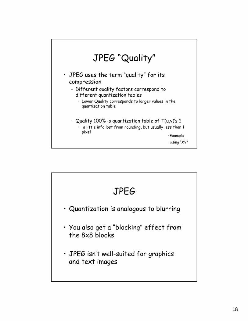
Example

8x8 block of pixels

DCT

C’(u,v) = C(u,v) ./ T(u,v)

-128

Example

Difference +128

IDCTC’(u,v) = C(u,v) .* T(u,v)

Reconstructed 8x8 pixels

18

JPEG “Quality”

• JPEG uses the term “quality” for its compression– Different quality factors correspond to

different quantization tables• Lower Quality corresponds to larger values in the

quantization table

– Quality 100% is quantization table of T(u,v)’s 1• a little info lost from rounding, but usually less than 1

pixel•Example

•Using “XV”

JPEG

• Quantization is analogous to blurring

• You also get a “blocking” effect from the 8x8 blocks

• JPEG isn’t well-suited for graphics and text images

19

JPEG Quantization Tables

Code for generating the Quantization tables used by JPEG

http://www.tux.org/pub/net/ftp.ee.lbl.gov/draft-ietf-avt-jpeg-02.txt

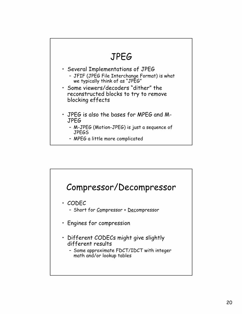
Color Image Compression via JPEG

⎥⎥⎥

⎦

⎤

⎢⎢⎢

⎣

⎡

⎥⎥⎥

⎦

⎤

⎢⎢⎢

⎣

⎡

−−−=

⎥⎥⎥

⎦

⎤

⎢⎢⎢

⎣

⎡

BGR

QIY

311.0523.0212.0321.0275.0596.0

114.0587.0299.0

Luminance

Color

Note: Quantization ofcolor info 2:1:1

yyyy

q

i

20

JPEG• Several Implementations of JPEG

– JFIF (JPEG File Interchange Format) is what we typically think of as “JPEG”

• Some viewers/decoders “dither” the reconstructed blocks to try to remove blocking effects

• JPEG is also the bases for MPEG and M-JPEG– M-JPEG (Motion-JPEG) is just a sequence of

JPEGS– MPEG a little more complicated

Compressor/Decompressor• CODEC

– Short for Compressor + Decompressor

• Engines for compression

• Different CODECs might give slightly different results– Some approximate FDCT/IDCT with integer

math and/or lookup tables

21

Graphics Interchange Format (GIF)

• short slide about GIF– another popular compression scheme

• GIF is lossless, uses Lempel-Ziv-Welch scheme, a variation on Huffman encoding

• However, some implementations of GIF only allow 255 colors– It quantizes the color– In this sense it is lossy

Image Compression Summary• Idea

– Reduce Redundancy– Maintain information

• Lossless Compression– Huffman Encoding– RLE (Mapping)– Predictive Encoding

• Lossy Compression– Quantization Step– Transform Coding

22

Image Compression Summary• Loss is due to quantization

– Gives much higher compression – Especially useful with transform coding

schemes• DCT is one of the most commonly used transforms

• JPEG– puts it all together (DCT, RLE, Huffman . . )

• There are criterions to compare CODECs– Objective

• Signal to Noise Ratio– Subjective

• Human-based rating system

Active Research Areas

• Mainly focused on video• Compression

– constant bit-rate compression– for networks

• Layered Compression• Quality of Service (QoS)

• Very low-bandwidth compression– teleconferencing over networking

23

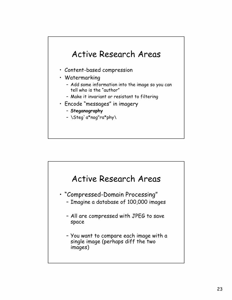
Active Research Areas

• Content-based compression• Watermarking

– Add some information into the image so you can tell who is the “author”

– Make it invariant or resistant to filtering• Encode “messages” in imagery

– Steganography– \Steg`a*nog"ra*phy\

Active Research Areas

• “Compressed-Domain Processing”– Imagine a database of 100,000 images

– All are compressed with JPEG to save space

– You want to compare each image with a single image (perhaps diff the two images)

24

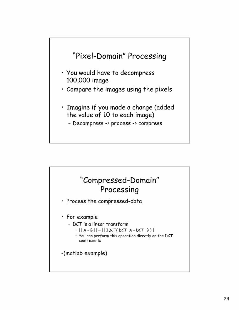
“Pixel-Domain” Processing

• You would have to decompress 100,000 image

• Compare the images using the pixels

• Imagine if you made a change (added the value of 10 to each image)– Decompress -> process -> compress

“Compressed-Domain”Processing

• Process the compressed-data

• For example– DCT is a linear transform

• || A – B || ~ || IDCT( DCT_A – DCT_B ) ||• You can perform this operation directly on the DCT

coefficients

-(matlab example)

25

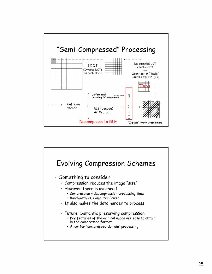
“Semi-Compressed” Processing

IDCT(Inverse DCT)on each block

De-quantize DCT coefficients

via Quantization “Table”C(u,v) = C’(u,v)*T(u,v)

T(u,v)

“Zig-zag” order Coefficients

RLE (decode)AC Vector

0Differentialdecoding DC component

Huffman decode

Decompress to RLE

Evolving Compression Schemes

• Something to consider– Compression reduces the image “size”– However there is overhead

• Compression + decompression processing time• Bandwidth vs. Computer Power

– It also makes the data harder to process

– Future: Semantic preserving compression• Key features of the original image are easy to obtain

in the compressed format• Allow for “compressed-domain” processing