Chapter 3 Image Compression Using Curvelet Transform 3.1 Introduction Compression techniques [8] that are based on modifying the transform of an image are considered here. In these techniques, a reversible, linear transform (such as transforms discussed in Chapter 2) is used to map the image into a set of transform coefficients, which are then quantized and coded. For most natural images, a significant number of the coefficients have small magnitudes and can be coarsely quantized with little image distortion. Fig. 3.1 shows a typical transform coding system. The decoder implements the inverse sequence of steps (with the exception of the quantization function) of the encoder, which performs three relatively straightforward operations: transformation, quantization, and coding. The goal of the transformation process is to decorrelate the pixels of image, or to pack as much information as possible into the smallest number of transform coefficients. The quantization stage then selectively eliminates or more coarsely quantizes the coefficients that carry the least information. These coefficients have the smallest impact on reconstructed image quality. The encoding process terminates by coding the quantized coefficients. 48

Welcome message from author
This document is posted to help you gain knowledge. Please leave a comment to let me know what you think about it! Share it to your friends and learn new things together.
Transcript
Chapter 3
Image Compression Using Curvelet Transform
3.1 Introduction
Compression techniques [8] that are based on modifying the
transform of an image are considered here. In these techniques, a
reversible, linear transform (such as transforms discussed in Chapter
2) is used to map the image into a set of transform coefficients, which
are then quantized and coded. For most natural images, a significant
number of the coefficients have small magnitudes and can be coarsely
quantized with little image distortion.
Fig. 3.1 shows a typical transform coding system. The decoder
implements the inverse sequence of steps (with the exception of the
quantization function) of the encoder, which performs three relatively
straightforward operations: transformation, quantization, and coding.
The goal of the transformation process is to decorrelate the pixels of
image, or to pack as much information as possible into the smallest
number of transform coefficients. The quantization stage then
selectively eliminates or more coarsely quantizes the coefficients that
carry the least information. These coefficients have the smallest
impact on reconstructed image quality. The encoding process
terminates by coding the quantized coefficients.
48

Fig. 3.1 A Transform coding (a) encoder and (b) decoder
In this chapter practical implementations of proposed
compression method is focused. The next section will briefly survey
existing methods, while section 3.3 briefs about new transform,
section 3.4 discusses the quantizer design for proposed compression
method, section 3.5 demonstrates the algorithm of new compression
technique and sections 3.6 and 3.7 explains the metrics and indexes
used to evaluate the performance. Finally, the superiority of proposed
technique over conventional methods is demonstrated.
3.2 Survey of Existing Methods
Past few years have produced abundant results in compression
techniques for images primarily for its wide spread usage in internet
technologies etc. Wavelet based compression of digital signals and
49

images have been a topic of interest for quiet sometime now. In many
hundreds of papers published [56-63] in journals throughout the
scientific and engineering disciplines, a wide range of tools and ideas
have been proposed and studied. Though wavelet based techniques
have proven their worth in number of fields the major drawback
associated with them are their inability to capture geometry of two
dimensional edges. Therefore, the field of image processing demands a
true 2-dimensional transform that can efficiently handle the intrinsic
geometrical structure that is the key in visual information. The next
section briefly describes the new transform that solves the problem of
capturing image edges.
3.3 New Multiscale Transform
Candes and Donoho [1] developed a new multi-scale transform
which they called as the curvelet transform . Motivated by the needs
of image analysis, it was nevertheless first proposed in the context of
objects f(x1; x2) defined on the continuum plane (x1,x2)∈R2. The new
transform is believed to capture image information more efficiently
than the wavelet transform by providing basis elements in addition to
possessing the qualities of wavelet. Basis functions in curvelets are
oriented at variety of directions and with variety of elongated shapes
with different aspect ratios. In particular, it was designed to represent
edges and other singularities along curves much more efficiently than
traditional transforms, i.e. using many fewer coefficients for a given
50

accuracy of reconstruction. Roughly speaking, to represent an edge to
squared error 1/N requires 1/N wavelets and only about 1/ N
curvelets. The details of curvelet transform are given in section 2.2 of
chapter 2.
3.4 Quantizer Design and Coding
The uniform quantizer is the most commonly used scalar
quantizer for transform based image compression due to its simplicity.
It is also known as a linear quantizer since its staircase input-output
response lies along a straight line(with a unit slope). Two commonly
used linear staircase quantizers are the midtread and the midrise
quantizers.
3.4.1 Existing Quantizer
From MATLAB tool box, it is observed that the quantizer is
defined as:
y=Q_T(x)
where: Q_T(x) = 0 , if |x|<T
Q_T(x) = sgn(x) * [x/T] , otherwise (3.1)
The input values for quantizer are created with evenly spacing
and bin size(T) is assumed as 0.1. The quantization curve is as shown
51

in Fig. 3.2(a). From the quantization curve, it can be said that the
above quantizer is midtread.
For decompression, de-quantized values are computed using
the following equation.
Dq=sgn(Q) * (abs(Q)+0.5)*T (3.2)
Where Q are quantizer output values and Dq are de-quantized values.
In the above equation 0.5 is chosen to get the de-quantized values at
the mid-point of each quantization bin. De-quantized real values are
shown in Fig. 3.2(b).
(a) (b)
Fig. 3.2. Existing Quantizer (a) Quantization curve (b) De-quantized
values.
It is known that the subinterval size of the midtread quantizer is
larger than the midrise quantizer. Hence for the uniformly distributed
input, the average quantization error of the midtread quantizer is
larger than that of midrise quantizer.
52

3.4.2 Proposed Quantizer
The two constraints to be considered while designing quantizer are
as follows:
1. Quantizer must have average quantization error as low as
possible.
2. De-quantized values must be exactly at the mid-point of each
quantization bin.
Since the source considered for compression application is uniformly
distributed, midrise quantizer is preferred, which satisfies the first
constraint.
To obtain the midrise quantizer and to satisfy second
constraint, the midtread quantizer equations are restructured as:
y=Q_T(x)
where: Q_T(x) = 0 , if |x|<T
Q_T(x) = sgn(x) * ([x/T]+K)*T , otherwise (3.3)
The input values for quantizer are created with evenly spacing and bin
size(T) is assumed as 0.1. Here K is a constant.
For decompression, de-quantized equation is modified as:
Dq=sgn(Q) * ([abs(Q)/T]-M)*T (3.4)
Where Q are quantizer output values, Dq are de-quantized values and
M is a constant.
53

The above equations are tested for different values of K and M.
For convenience the quantization and de-quantization curves for three
different combinations of K and M are shown in Figs. 3.3, 3.4 and 3.5.
(a) (b)
Fig. 3.3 Proposed Quantizer with K=0.6 and M=0.5 (a) Quantization
curve (b) De-quantized values.
In Fig. 3.3 , it is observed that for K=0.6 and M=0.5 the
quantization and de-quantization curves are not efficient and the de-
quantized values are not at the mid-point of each quantization bin.
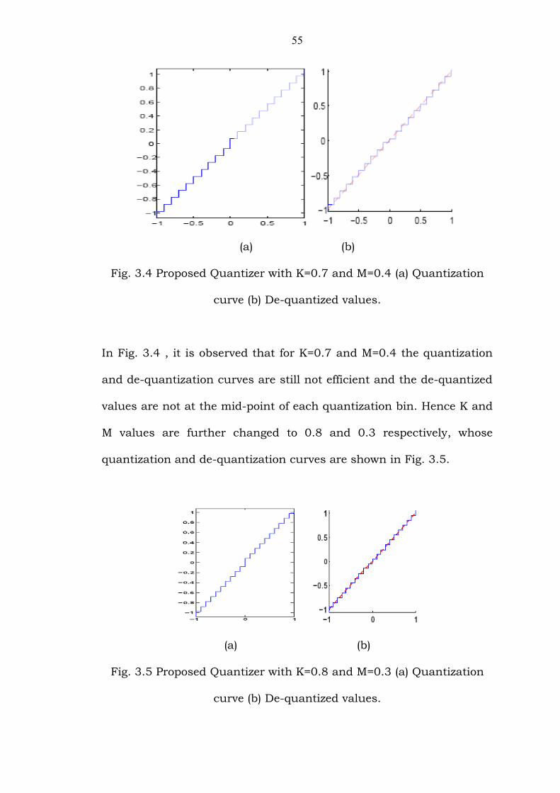
Hence K and M values are changed to 0.7 and 0.4 respectively, whose
quantization and de-quantization curves are shown in Fig. 3.4.
54
(a) (b)
Fig. 3.4 Proposed Quantizer with K=0.7 and M=0.4 (a) Quantization
curve (b) De-quantized values.
In Fig. 3.4 , it is observed that for K=0.7 and M=0.4 the quantization
and de-quantization curves are still not efficient and the de-quantized
values are not at the mid-point of each quantization bin. Hence K and
M values are further changed to 0.8 and 0.3 respectively, whose
quantization and de-quantization curves are shown in Fig. 3.5.
(a) (b)
Fig. 3.5 Proposed Quantizer with K=0.8 and M=0.3 (a) Quantization
curve (b) De-quantized values.
55
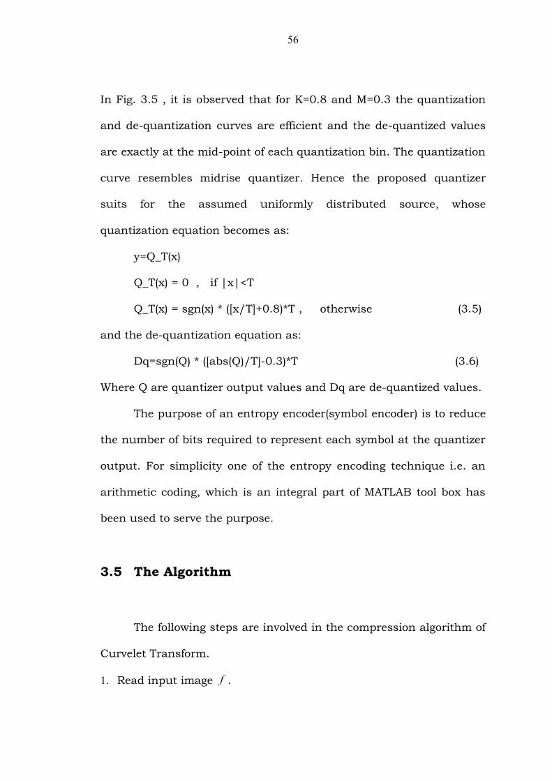
In Fig. 3.5 , it is observed that for K=0.8 and M=0.3 the quantization
and de-quantization curves are efficient and the de-quantized values
are exactly at the mid-point of each quantization bin. The quantization
curve resembles midrise quantizer. Hence the proposed quantizer
suits for the assumed uniformly distributed source, whose
quantization equation becomes as:
y=Q_T(x)
Q_T(x) = 0 , if |x|<T
Q_T(x) = sgn(x) * ([x/T]+0.8)*T , otherwise (3.5)
and the de-quantization equation as:
Dq=sgn(Q) * ([abs(Q)/T]-0.3)*T (3.6)
Where Q are quantizer output values and Dq are de-quantized values.
The purpose of an entropy encoder(symbol encoder) is to reduce
the number of bits required to represent each symbol at the quantizer
output. For simplicity one of the entropy encoding technique i.e. an
arithmetic coding, which is an integral part of MATLAB tool box has
been used to serve the purpose.
3.5 The Algorithm
The following steps are involved in the compression algorithm of
Curvelet Transform.
1. Read input image f .
56

2. Apply the 2D FFT and obtain Fourier samples
1 2 1 2ˆ[ , ], / 2 , / 2.f n n n n n n− ≤ <
3. For each scale j and angle l , form the product , 1 2 1 2ˆ[ , ] [ , ].j lU n n f n n%
4. Wrap this product around the origin and obtain
, 1 2 , 1 2ˆ[ , ] ( )[ , ],j l j lf n n W U f n n=% % where the range for 1n and 2n is now
1 1,0 jn L≤ < and 2 2,0 jn L≤ < (for θ in the range ( / 4, / 4)π π− ).
5. Apply the inverse 2D FFT to each ,j lf% , hence collecting the discrete
coefficients ( , , )Dc j l k .
6. Quantize the coefficients with the proposed quantizer.
7. Entropy code the quantizer outputs.
8. Apply inverse operations to the result of step 7.
Based on the algorithm stated above, a compression technique has
been developed for images of different sizes, which is tested using
Curvlab[16] and MATLAB tools. The algorithm developed is working to
a satisfaction and results are encouraging in case of curvelets.
3.6 Compression Metrics
The basic compression metric used to evaluate the performance
of the compression algorithm is the compression ratio, which is
defined as:
57

( )(%)( )
Output file size bytesCompression ratioInput file size bytes
=
Rate is another metric used to evaluate the performance of the
compression algorithm, that gives the number of bits per pixel
(bpp)used to encode an image and is defined as:
8*( ( ))( )( )
Output file size bytesRate bppInput file size bytes
=
3.7 Performance Index
In the Objective fidelity criteria Mean Square Error(MSE), Signal
to Noise Ratio(SNR) and Peak Signal to Noise Ratio(PSNR) are used to
evaluate the quality of the decompressed image of an algorithm. MSE
has some problem when images with different types of degradation are
compared. The PSNR measure is superior to other measures such as
SNR as it uses a constant value in which to compare the noise against
instead of a fluctuating signal as in SNR. This allows PSNR values
received to be treated more meaningfully when quantifiably comparing
different image coding algorithms. Hence PSNR is used which is
defined as:
1 2
21 2
2
1 1
max( ( , ))10 log10[ ( , ) ( , )]
M M
i j
M M f i jpsnr dBf i j f i j
= =
× ×=′−∑ ∑ (3.7)
where M1 and M2 are the size of the image. ( , )f i j is the original image,
( , )f i j′ is the decompressed image.
58

3.8 Simulations
In the simulation, various images like plain(Barbara), Building
and Textured images have been selected for compression. The results
are presented in Figs. 3.6 to 3.14 and in Tables 3.1 to 3.3. The results
indicate that there exists a qualitative difference between the methods
considered for compression and reconstruction of image under test.
The following observations are made from the results.
1. The curvelet with proposed quantizer algorithm enjoys superior
compression ratio over wavelet with existing quantizer, curvelet
with existing and wavelet with proposed quantizer algorithms.
The performance is judged mainly through visual clarity and
through PSNR.
2. The curvelet with proposed quantizer reconstruction displays
higher sensitivity even at higher compression ratios.
3. In case of plain(Barbara) image the curvelet with proposed
quantizer performs better at all compression ratios compared to
other algorithms, where as in case of Building and Textured
images at low compression ratios curvelet with existing
quantizer performs better compared to other algorithms, but at
higher compression ratios curvelet with proposed quantizer
outperforms the other algorithms irrespective of image.
59

(a)
(b) (c) (d) (e)
Fig. 3.6 Barbara image for compression ratio of 1:20 (a) Original
image (b) Wavelet with existing quantizer (c) Curvelet with existing
quantizer (d) Wavelet with proposed quantizer (e) Curvelet with
proposed quantizer.
60
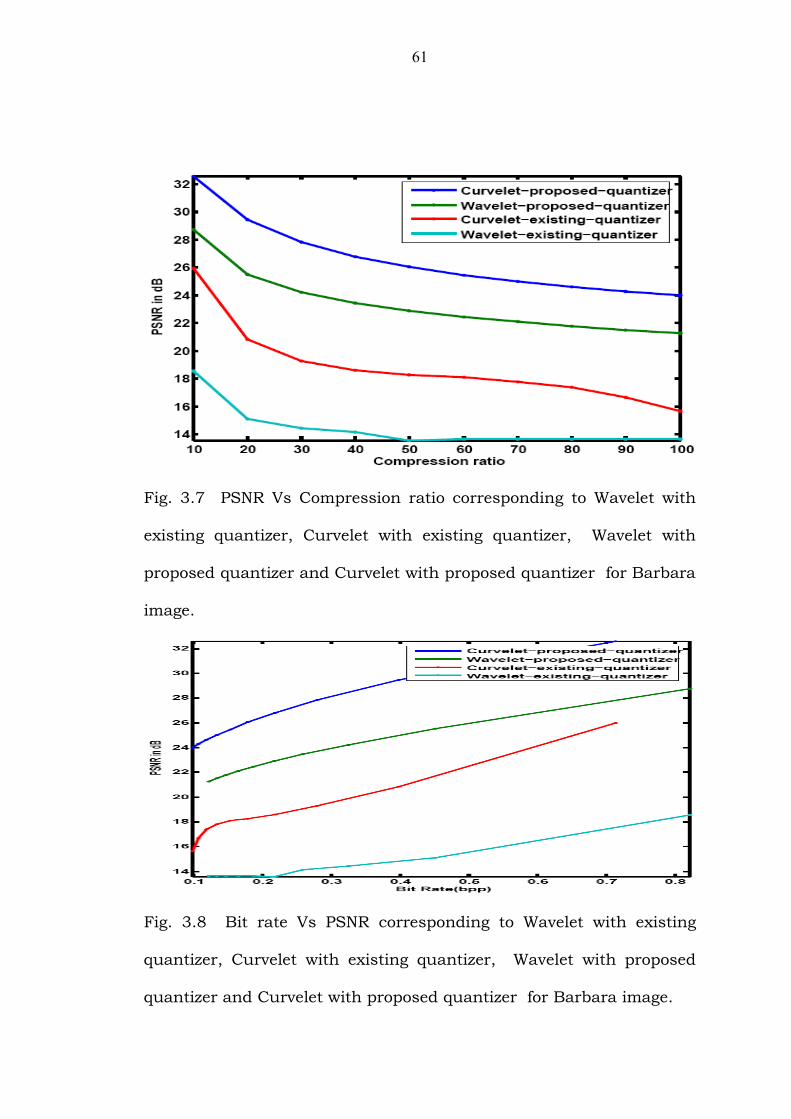
Fig. 3.7 PSNR Vs Compression ratio corresponding to Wavelet with
existing quantizer, Curvelet with existing quantizer, Wavelet with
proposed quantizer and Curvelet with proposed quantizer for Barbara
image.
Fig. 3.8 Bit rate Vs PSNR corresponding to Wavelet with existing
quantizer, Curvelet with existing quantizer, Wavelet with proposed
quantizer and Curvelet with proposed quantizer for Barbara image.
61

Table 3.1 PSNR Vs Compression ratio for various algorithms w.r.t.
Barbara image.
S.No Compression
ratioPSNR in dB(Barbara image)
Wavelet
With existing
quantizer
Curvelet
With existing
quantizer
Wavelet
With proposed
quanizer
Curvelet
With proposed
quantizer1 10 18.5611 25.9800 28.7499 32.61062 20 15.0924 20.8571 25.5371 29.48963 30 14.4269 19.2967 24.2425 27.87194 40 14.1493 18.6013 23.4729 26.81125 50 13.5877 18.2636 22.9075 26.04766 60 13.6517 18.1034 22.4776 25.47637 70 13.6520 17.8048 22.1051 25.00488 80 13.6514 17.4066 21.7726 24.62829 90 13.6510 16.6934 21.5213 24.292910 100 13.6500 15.6489 21.2750 24.0100
62

(a)
(b) (c) (d) (e)
Fig. 3.9 Building image for compression ratio of 1:100 (a) Original
image (b) Wavelet with existing quantizer (c) Curvelet with existing
quantizer (d) Wavelet with proposed quantizer (e) Curvelet with
proposed quantizer.
63

Fig. 3.10 PSNR Vs Compression ratio corresponding to Wavelet with
existing quantizer, Curvelet with existing quantizer, Wavelet with
proposed quantizer and Curvelet with proposed quantizer for Building
image.
Fig. 3.11 Bit rate Vs PSNR corresponding to Wavelet with existing
quantizer, Curvelet with existing quantizer, Wavelet with proposed
quantizer and Curvelet with proposed quantizer for Building image.
64
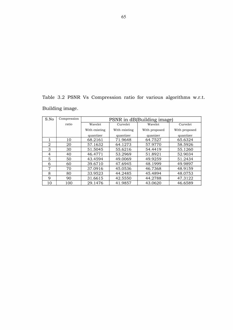
Table 3.2 PSNR Vs Compression ratio for various algorithms w.r.t.
Building image.
S.No Compression
ratioPSNR in dB(Building image)
Wavelet
With existing
quantizer
Curvelet
With existing
quantizer
Wavelet
With proposed
quanizer
Curvelet
With proposed
quantizer1 10 68.2161 71.9648 64.7527 65.63242 20 57.1632 64.1273 57.9770 58.59263 30 51.5045 55.6216 54.4419 55.12604 40 46.4771 53.2969 51.8921 52.90345 50 43.4594 49.0069 49.9259 51.24346 60 39.6710 47.6945 48.1999 49.98977 70 37.0916 45.0536 46.7368 48.91598 80 33.9523 44.2485 45.4894 48.07539 90 31.6615 42.5550 44.2788 47.312210 100 29.1476 41.9857 43.0620 46.6589
65

(a)
(b) (c) (d) (e)
Fig. 3.12 Textured image for compression ratio of 1:100 (a) Original
image (b) Wavelet with existing quantizer (c) Curvelet with existing
quantizer (d) Wavelet with proposed quantizer (e) Curvelet with
proposed quantizer.
66

Fig. 3.13 PSNR Vs Compression ratio corresponding to Wavelet with
existing quantizer, Curvelet with existing quantizer, Wavelet with
proposed quantizer and Curvelet with proposed quantizer for
Textured image.
Fig. 3.14 Bit rate Vs PSNR corresponding to Wavelet with existing
quantizer, Curvelet with existing quantizer, Wavelet with proposed
quantizer and Curvelet with proposed quantizer for Textured image.
67
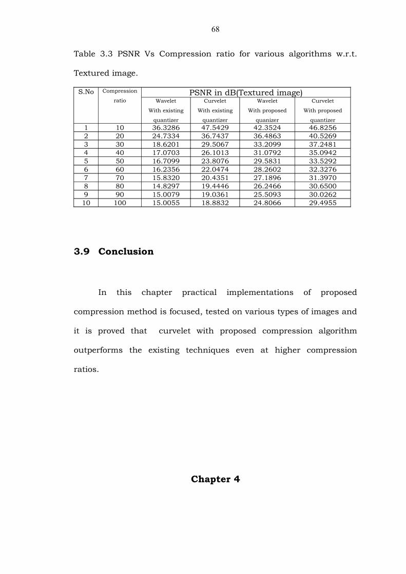
Table 3.3 PSNR Vs Compression ratio for various algorithms w.r.t.
Textured image.
S.No Compression
ratioPSNR in dB(Textured image)
Wavelet
With existing
quantizer
Curvelet
With existing
quantizer
Wavelet
With proposed
quanizer
Curvelet
With proposed
quantizer1 10 36.3286 47.5429 42.3524 46.82562 20 24.7334 36.7437 36.4863 40.52693 30 18.6201 29.5067 33.2099 37.24814 40 17.0703 26.1013 31.0792 35.09425 50 16.7099 23.8076 29.5831 33.52926 60 16.2356 22.0474 28.2602 32.32767 70 15.8320 20.4351 27.1896 31.39708 80 14.8297 19.4446 26.2466 30.65009 90 15.0079 19.0361 25.5093 30.026210 100 15.0055 18.8832 24.8066 29.4955
3.9 Conclusion
In this chapter practical implementations of proposed
compression method is focused, tested on various types of images and
it is proved that curvelet with proposed compression algorithm
outperforms the existing techniques even at higher compression
ratios.
Chapter 4
68
Related Documents