Image change detection from difference image through deterministic simulated annealing

THEORETICAL ADVANCES

Image change detection from difference imagethrough deterministic simulated annealing

Gonzalo Pajares Æ Jose J. Ruz Æ Jesus M. de la Cruz

Received: 9 March 2007 / Accepted: 14 February 2008 / Published online: 14 March 2008

� Springer-Verlag London Limited 2008

Abstract This paper proposes an automatic method based

on the deterministic simulated annealing (DSA) approach for

solving the image change detection problem between two

images where one of them is the reference image. Each pixel

in the reference image is considered as a node with a state

value in a network of nodes. This state determines the

magnitude of the change. The DSA optimization approach

tries to achieve the most network stable configuration based

on the minimization of an energy function. The DSA scheme

allows the mapping of interpixel contextual dependencies

which has been used favorably in some existing image

change detection strategies. The main contribution of the

DSA is exactly its ability for avoiding local minima during

the optimization process thanks to the annealing scheme.

Local minima have been detected when using some opti-

mization strategies, such as Hopfield neural networks, in

images with large amount of changes, greater than the 20%.

The DSA performs better than other optimization strategies

for images with a large amount of changes and obtain similar

results for images where the changes are small. Hence, the

DSA approach appears to be a general method for image

change detection independently of the amount of changes. Its

performance is compared against some recent image change

detection methods.

Keywords Image change detection � Difference images �Simulated annealing � Markov random fields

1 Introduction

The automatic image change detection methods are suit-

able for many vision computer applications [30]. For

instance, video surveillance [7, 26, 31,36–38 ], analysis of

multitemporal remote sensing images [3–5], tracking sys-

tems of moving objects [24], medical diagnosis [2] or

driver assistance systems [ 12] among others.

The goal is to identify the changed pixels between two

images captured at different time periods; one of the

images is the reference. Different factors cause changes:

appearance or disappearance of objects, motion of objects

relative to the background, shape change of objects or

environment modifications (buildings, fires, etc.) [30].

The techniques based on background modeling are out of

the scope of this paper. The reader is referred to references

[7, 8, 30].

According to the classification proposed by Radke et al.

[30] there are several major types of change detection

schemes for detecting the difference between two images,

I1 and I2, of the same scene captured at different time

periods. In Pajares [27] is included an introduction about

some of the above schemes.

1. Simple differencing: Given a pixel location (x, y), the

difference associated to this pixel is given as: D(x, y) = |I2

(x, y) - I1(x, y)|. A change is detected at this location if

D(x, y) is large as compared to a threshold T. So, under this

approach the goal is to compute the threshold T. A study

about some histogram-based automatic thresholding algo-

rithms for choosing T is provided in Rosin and Ioannidis

[31]. In Wu et al. [38] and Lu and Suganthan [26] some

G. Pajares (&)

Dpto. Ingenierıa del Software e Inteligencia Artificial,

Facultad de Informatica, Universidad Complutense,

28040 Madrid, Spain

e-mail: [email protected]

J. J. Ruz � J. M. de la Cruz

Dpto. Arquitectura de Computadores y Automatica,

Facultad de Informatica, Universidad Complutense,

28040 Madrid, Spain

123

Pattern Anal Applic (2009) 12:137–150

DOI 10.1007/s10044-008-0110-5

improvements are proposed in order to solve some draw-

backs of some thresholding methods.

2. Significance and hypothesis tests models: A change is

declared at a given pixel location (x, y) based on two

competing hypotheses: the null hypothesis H0 or the

alternative hypothesis H1, corresponding to no-change and

change decision respectively. Aach and Kaup [1] assume

that the difference image D(x, y) is characterized by two

zero-mean Gaussian distributions with variances r02 and r1

2

for H0 and H1 respectively. The goal of this approach is

to estimate a changed binary mask Q given D. Bruzzone

and Fernandez [5] estimate the parameters of the mixture

distribution at each pixel location p(D(x,y)), which is

modeled as

p Dðx; yÞð Þ ¼ p Dðx; yÞ H0jð ÞP H0ð Þ þ p Dðx; yÞ H1jð ÞP H1ð Þð1Þ

The conditional estimations p(D(x,y)|H0), p(D(x,y)|H1)

and P(H0), P(H1) are carried out by using the iterative

expectation maximization (EM) algorithm [9] until the

convergence. They assume Gaussian distributions for

the a priori probabilities, where the parameters to be

estimated are the means l0, l1 and variances r12, r0

2,

respectively. The initial values of the estimates are

determined from D. In this approach an interpixel spatial

relation is applied in order to achieve consistency during

the estimation.

3. Predictive models: There are spatial and temporal

models that exploit the close relationships between nearby

pixels. In the spatial models, given two blocks of two

intensity values, a polynomial function of the pixel

coordinates is fitted to the intensity values. Hsu et al. [16]

use likelihood ratio tests using constant, linear or qua-

dratic models for the image blocks. A change is detected if

the corresponding blocks are best fit by different poly-

nomial coefficients. In temporal models Jain and Chau

[17] assumed each pixel was identically and indepen-

dently distributed according to the same Gaussian

distribution related to the past by the same coefficient.

They derive maximum likelihood estimates of the mean,

variance and correlation coefficient at each point in time.

A change is detected when the image intensities are

independent.

4. Shading models: Based on linear dependencies was

originally proposed by Durucam and Ebrahimi [11]. Given

the pixel location (x, y) a vector of n neighboring intensity

pixels, x = {x1,..., xn} is built. This pixel is a unchanged/

changed pixel in the next frame if x and the new vector y =

{y1,..., yn} built from the new frame are linearly

dependent/independent. Assuming that x, y are two lin-

early dependent vectors with no components zero, then

the ratio of their components is constant, i.e., x1/y1 = x2/

y2 = �� = xn/yn = constant. In a 8-connected neighbor-

hood this is expressed as: I1(x - 1, y - 1)/I2(x - 1,y - 1)

= I1(x - 1, y)/I2(x - 1, y) = �� = I1(x + 1, y + 1)/

I2(x + 1, y + 1) = constant. Hence, in the 8-connected

neighborhood, under the linear dependence, the variance is

zero, as one can infer from the variance definition,

r2ðx; yÞ ¼ 1n�1

Pðx;yÞ2A I1ðx; yÞ=I2ðx; yÞ � lðx; yÞð Þ2; where

lðx; yÞ ¼ 1n

Pðx;yÞ2A I1ðx; yÞ=I2ðx; yÞð Þ ¼ constant and n is

the number of members in the neighborhood A of (x, y),

i.e., eight in this approach. Under linear independence, the

variance should not be zero. Skifstad and Jain [32] and Liu

et al. [24] apply this model and determine a threshold

empirically. Considering that the intensity image is the

product of the illumination Il(x, y) from the light source in

the scene and the reflectance Ir(x, y) of the object surface to

which (x, y) belongs, the intensity can be expressed as I(x,

y) = Il(x, y)Ir(x, y). The reflectance component depends

only on the intrinsic properties of the object surface.

Hence, given two images I1, I2 and assuming the illumi-

nation constant, a change is detected based on the

reflectance components.

5. Background modeling: Given two consecutive frames

Ii(x, y) and Ii-1(x, y), Chang et al. [7] determine that a pixel

has changed if |Ri (x, y)| [ T otherwise it belongs to the

background. Ri is computed as Ri(x, y) = Mi-1(x, y)

Di(x, y); Di is the difference image between Ii and Ii-1.

The first time Mi-1 is set to zero, next during the following

steps Ri is assigned to Mi. Carlotto [6] models the back-

ground as a Gaussian distribution computing its

representative mean value and covariance matrix. A pixel

is classified as changed if the Mahalanobis distance [9]

between its difference value and the mean is large. Para-

gios and Deriche [29] and Stauffer and Grimson [35]

assume that changed pixels belong to moving objects

otherwise they are unchanged belonging to the background.

A mixture probability density function is estimated

assuming two classes according to the above consideration.

6. Change mask consistency: As reported in Radke et al.

[30] the methods using thresholding give noisy results,

isolated changed/unchanged pixels, holes or jagged

boundaries. To overcome this drawback most methods try

to apply a consistency criterion. One important framework

used by these methods to enforce the contextual informa-

tion is Markov Random Fields (MRF). Under the MRF

framework, a probability density function (PDF) is defined

for each pixel location in the difference image D. The PDF

generally follows the Gibbs distribution and embeds an

energy term. The goal of the approaches based on change

mask consistency is to maximize the PDF at each pixel

location or equivalently minimize the energy. Bruzzone

and Fernandez-Prieto [4], Aach and Kaup [1], Kasetkasen

and Varshney [19], Liu [23] and Liu et al. [25] basically

compute two energy terms. Previously each pixel is labeled

138 Pattern Anal Applic (2009) 12:137–150

123

as changed/unchanged according to a thresholding tech-

nique applied to the difference image D. A first energy

term is computed from the joint density function of the

pixel values in D given the label. This term takes into

account a kind of self-information for each pixel location.

A second energy term is computed through the interactions

between a pixel and its neighbors taking into account their

labels. This term in the above approaches is termed the

consistency term. Assuming a random field defined by the

PDFs, we can see in the above approaches that the energy

for each pixel is computed based only on the own pixel and

its neighbors, out of the neighborhood the contribution to

the energy of the pixels is null. This implies that the ran-

dom fields fulfil the so called Markov condition for spatial

descriptions as the images, i.e., the field is termed a MRF.

The MRF is an approach which has been broadly used in

image analysis [10]. Liu et al. [25] compute the consis-

tency by applying the mean field theory (MFT) which

assumes that the impacts from the neighbors can be

approximated by an average field. In Pajares [27] the

change detection problem is focused minimizing an energy

function through the analog hopfield neural network

(HNN) paradigm. Under this paradigm, the energy function

assumes a trade-off between the self-information and the

consistency. Also, under the HNN approach the consis-

tency is extended so that the interactions in a neighborhood

around a pixel location are based not only in the labels but

also in the joint density function values of the neighbors,

i.e., this implicitly assumes the Markovian condition. This

extension and the analog properties of the HNN paradigm

make of this method a valid approach for the set of images

tested as compared with other existing image change

detection strategies.

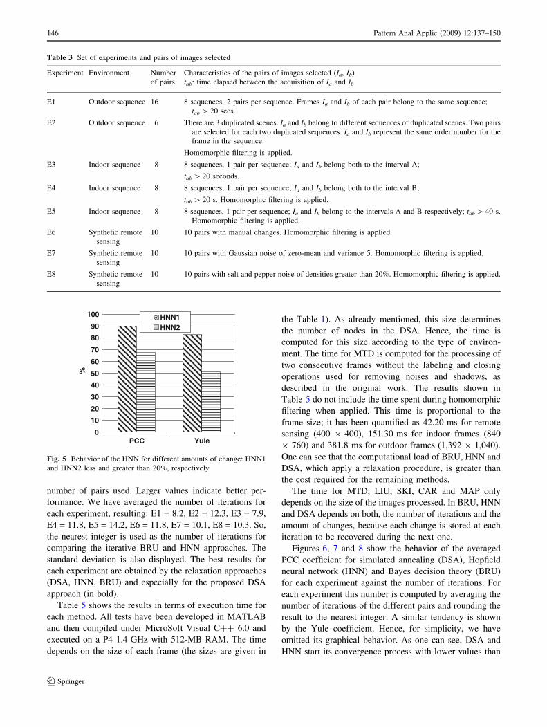
Unfortunately, through additional experiments we have

verified that for images where the amount of changes

surpasses the 20% the performance of the HNN approach

decreases (see Fig. 5 and related comments in Sect. 3.3).

This is because there is an important number of these

difference images in which the energy falls in local minima

that are not global optimum. This behavior of the Hopfield

neural network is reported in Haykin [15]. The change

mask consistency approaches, involving both contextual

and self information, perform favorably. The deterministic

simmulated annealing (DSA) is also an energy optimiza-

tion based approach which can embed contextual and self

information with the advantage that it can avoid local

minima. Indeed, according to Geman and Geman [13] and

reproduced in Haykin [15] when the temperature involved

in the simulated annealing process satisfies some con-

straints (explained in the Sect. 2.5) the system converges to

the minimum global energy which is controlled by the

annealing scheduling instead of the nonlinear first-order

differential equation used in HNN. This is the main

difference of the proposed DSA technique with respect to

the HNN approach.

In Kasetkasen and Varshney [19] the stochastic simu-

lated annealing (SSA) is used to minimize the energy under

the MRF framework. The results are binary labels indi-

cating only changed/unchanged pixels. In Duda et al. [9] it

is reported that SSA is slow due to its discrete nature as

compared to the analog nature of the DSA.

In summary, we focus on the DSA approach, making the

main contribution of this paper, because of the following

set of advantages: (a) the contextual and self information

can be mapped under an energy function; (b) the annealing

scheduling allows avoiding local minima; (c) the optimi-

zation process corrects a posteriori the initial errors derived

from a thresholding approach and (d) the analog nature

allows to obtain the strength of the change for each pixel

location.

The paper is organized as follows. In Sect. 2, the DSA

process is described including the mapping of the self-

information and consistencies. The performance of the

method is illustrated in Sect. 3, where a comparative

analysis against other existing image change detection

strategies is carried out. Finally, in Sect. 4, there is a dis-

cussion of some related topics.

2 Deterministic simulated annealing process

We build a network of nodes, so that each pixel location

(x, y) in the reference image or equivalently in the differ-

ence image D is associated to a node i. The node i is

interconnected to the node j through a symmetric synaptic

weight wij which is to be defined later. Moreover, each

node i has associated a state value si which will be set

through an activation function. A commonly activation

function is the hyperbolic tangent one, which is bounded by

-1 and +1 values [15]. Because of the analog nature of the

DSA approach and taking into account the above limits, the

si values range in the continuous interval [-1, + 1], where

-1 and +1 indicate, from our point of view, a secure

unchanged and changed pixels respectively. Other values

in [-1, + 1] measure the degree of the change. The states

are updated after each step t. Based on the change mask

consistency strategies described in the point 6 of the

introduction, we assume that our method falls under the

MRF framework [10]; where instead of maximizing a PDF

we minimize an energy function, which is equivalent. The

updating process for each node i, is carried out through the

DSA optimization approach assuming that the energy must

be minimum. This is carried out through a regularization

coefficient which computes the consistency between the

states of the nodes in a given neighborhood and a data

coefficient which computes the consistency between the

Pattern Anal Applic (2009) 12:137–150 139

123

difference image data values in D also in the same neigh-

borhood. This is the neighborhood which characterizes the

MRF as stated in the previous section. Both, regularization

and data coefficients represent a trade-off between them, so

that they can be mutually compensated. The own state

value (i.e., the self-information) is mapped during the DSA

updating process. A network initialization process is

required before the updating process is triggered. These

issues are addressed in the following subsections.

2.1 Network initialization

The network initialization is carried out by exploiting the

characteristics of the difference image, D. We use the

initialization strategy, described in Bruzzone and Fernan-

dez-Prieto [5]. From the histogram h(D) of the difference

image, we compute the minimum and maximum values

m = min{D} and M = max{D} and then two thresholds T0

and T1 as T0 = MD (1 - a) + am and T1 = MD (1 + a)

-am, where MD is the middle value of h(D), i.e., MD ¼12

mþMð Þ; a 2 ð0; 1Þ; set to 0.5 in this paper. Generally, m

is zero because the most typical case is that some pixel is

unchanged.

The thresholds T0 and T1 divide the histogram into three

zones, Z1, Z2 and Z3 as follows: Z1 = {D(x,y)|m B D(x,y)

B T0}; Z2 = {D(x, y)| T0 \ D(x, y) B T1 } and Z3 =

{D(x, y)|T1 \ D(x, y) B M}. Z1/Z3 define two ranges where

pixels belonging to D can be identified as unchanged/changed

respectively. Z2 defines the ambiguous zone, in which pixels

cannot be identified as either changed or unchanged.

Based on the above, each node i is initialized with a

state value as follows:

st¼0i ¼

�1 if Dðx; yÞ 2 Z1

þ1 if Dðx; yÞ 2 Z3

�1 or þ 1(randomly) if Dðx; yÞ 2 Z2

8<

:ð2Þ

A node with its state value equal to -1/+1 is clearly

identified as unchanged/changed. Nodes with values rang-

ing in (-1, +1] are changed nodes with different strengths.

The states associated to Z2 are randomly initialized through

a uniform distribution.

2.2 Statement of problem

The goal of the proposed method is to determine the

magnitude of the change of each node from the initial state

values and by applying consistency through the data and

regularization coefficients and also through the own state

value. This is achieved basically through the DSA opti-

mization process. The process must evolve by increasing

the state value of a changed node towards +1 and

decreasing the state of any unchanged node towards -1.

This implies that any node (changed or unchanged) can

modify its state, but also they could stay with stable states

even if they are changed nodes.

Suppose a network with N nodes. The simulated

annealing optimization problem is: modify the analog

values si so as to minimize the energy [9, 15]

E ¼ � 1

2

XN

i¼1

XN

j¼1

wijsisj ð3Þ

where wij is the symmetric weight interconnecting two

nodes i and j and can be positive or negative ranging in

[-1, +1]. Each wij determines the influence that the node j

exerts on i trying to modify the state si, Fig. 1 displays how

this influence is exerted through the consistencies mapped

as data and regularization coefficients. According to Duda

et al. [9] the self-feedback weights must be null (i.e., wii

= 0). The DSA approach tries to achieve the most network

stable configuration based on the energy minimization.

From (3) one can see that this expression requires the

x

wij= +1

wik= −1

C

R

x

y -1 -1 1

-1 1 1

-1 -1 1

C

R

y -1 -1 1

-1 1 1

-1 -1 1

differenceimage

C

R

x

y

02550

0

0 0

states ≡ si

datainformation ≡ r (i)

i

i

Ni8

255

255255

j

k

j

k dik= −1

dij= +1

cik= −1

cij= +1

Fig. 1 Pedagogical example

displaying the influence exerted

by nodes j and k on node i


123

computation of wij and the states of the nodes si and sj;wij is

obtained as a weighted sum of the regularization and the

data coefficients, it involves two nodes based on a neigh-

borhood relation; si and sj are obtained after the

corresponding updating process.

2.3 Data coefficient

In Pajares [27] also a relation among the pixels is described

by defining a kind of data consistency. We map the data

information following Bruzzone and Fernandez-Prieto [5]

according to the description in the significance and

hypothesis tests models. Given the difference image D we

formulate the Bayes rule for each pixel location (x, y)

considering the H0 and H1 hypotheses as follows:

P Hk Dðx; yÞjð Þ ¼ p Dðx; yÞ Hkjð ÞPðHkÞp Dðx; yÞð Þ ð4Þ

where p(D(x,y)) is given in the Eq. (1) and the conditional

probabilities p(D(x,y)|Hk) and the a priori P(Hk) are esti-

mated through the EM algorithm. The initialization is

carried out through the process described in the Sect. 2.1.

A node in the network is declared as changed or

unchanged if it is associated to H1 or H0, respectively. This

membership assignment is carried out according to the

following equation,

Hn ¼ arg maxHn2 H0;H1f g

P Hn Dðx; yÞjð Þf g

¼ arg maxHn2 H0;H1f g

PðHnÞp Dðx; yÞ Hnjð Þf g ð5Þ

From (5) a data map is built for each pixel location, i.e., for

each node (pixel) i : (x, y) in the network. According to

the maximum value in (5), H0 or H1 is selected, i.e., n = 0

or 1 consequently. So, for each node i we compute the data

information r(i) as follows:

rðiÞ ¼ �P H0 DðiÞjð Þ if Hn ¼ H0

þP H1 DðiÞjð Þ if Hn ¼ H1

�

ð6Þ

Each node i has associated its m-connected neighborhood,

Nim, m is set to 8 in this paper. The data consistency

between nodes i and j in the network is measured through a

similarity measurement by the data coefficient dij as

follows:

dij ¼1� rðiÞ � rðjÞj j j 2 Nm

i ; j 6¼ i0 j 62 Nm

i

�

ð7Þ

From (7) we can see that dij ranges in [-1, +1] where the

lower/higher limit means minimum/maximum data con-

sistency, respectively. Hence, according to the Eq. (4) the

data coefficient measures how similar are the probabilities

of change for the nodes i and j. Indeed, assume that i and j

are both changed or unchanged nodes simultaneously with

identical magnitude in the difference image D and j [ Nim, j

= i; hence both are associated to the same hypothesis H0

or H1 respectively and r(i) = r(j). This implies that dij = 1

when i and j are of the same category and magnitude. Now

consider that they belong to different categories, i.e., i is

changed and j unchanged or viceversa with j [ Nim, j = i.

Assume that i is with H0 and j with H1 and they both take

the maximum values, i.e., P(H0|D(i)) = 1 and P(H1|D(j)) = 1;

according to (6) r(i) = -1 and r(j) = +1. The same

is applicable if i is with H1 and j with H0. This leads to

dij = -1 which indicates maximum inconsistency. Any

similarity measurement and norm could be used in the

Eq. (7).

2.4 Regularization coefficient

In Bruzzone and Fernandez-Prieto [5], Aach and Kaup [1],

Kasetkasen and Varshney [19] and Pajares [27] a relation

among the pixels is described by defining a kind of con-

textual consistency. Given the node i with its state value sit

and a set of nodes j, where j [ Nim with state values sj

t. The

node i achieves a high consistency when sit and sj

t have both

similar values. This is mapped into the regularization

coefficient cij through a similarity measurement as follows:

cij ¼ 1� st�1i � st�1

j

��

�� j 2 Nm

i

0 j 62 Nmi

(

ð8Þ

From (8) we can see that cij varies with the iteration and

ranges in [-1, +1] where the lower/higher limit means

minimum/maximum consistency, respectively. As in dij,

any similarity measurement and norm could be used in the

Eq. (8). As one can see from the Eq. (8), the cij values are

computed taking into account only the previous state

values.

2.5 Simulated annealing: updating process

From (7) and (8) we combine dij and cij as the averaged

sum, taking into account the signs,

Wij ¼ cdij þ ð1� cÞcij; wij ¼ sgn Wij

� �� vþ1Wij;

sgn Wij

� �¼ �1 Wij� 0

þ1 Wij [ 0

� ð9Þ

c [ [0,1] represents the trade-off between both coefficients.

After a set of experiments we have chosen c = 0.65 because

the state values are already involved directly in the energy

computation through the Eq. (3). This avoids the over

contribution of the state values in the energy value; sgn is

the signum function and v is the number of negative values

in the set C : {Wij, si, sj}, i.e., given S � q 2f C=q\0g �C; v ¼ cardðSÞ: The expressions in (9) take into account

that the energy must achieve its minimum value for stable

states.


123

Figure 1 shows a pedagogical example about the influ-

ence exerted, through the weights wij, wik, on node i by the

nodes j and k according to the Eq. (9) from the data and

regularization coefficients dij, dik. This is achieved from the

difference image of size RxC based on the neighborhood

Ni8. As one can see the influence exerted by the nodes j and

k is +1 and -1 respectively, this is because of the similarity

of j and dissimilarity of k with respect the node i.

The simulated annealing process was originally deve-

loped in Kirkpatrick et al. [21] and Kirkpatrick [20]. In this

paper we have implemented the approach described in

Duda et al. [9] and Haykin [15]. According to Duda et al.

[9] the DSA process is computationally faster than the SSA

process. We have verified this assertion by implementing

both versions (deterministic and stochastic), obtaining very

similar solutions and identical performance in terms of

correct changed or unchanged nodes. Nevertheless, the

deterministic version has been faster than the stochastic, by

exactly two orders of magnitude. This agrees with Duda

et al. [9]. Moreover, we have not found problems to reach

the global minimum under the deterministic version; this is

because the DSA is initially guided (not randomly) during

the initialization.

Following the notation in Duda et al. [9], let lti ¼P

j wijstj be the force exerted on node i by the other nodes j

[ Nim at the iteration t; then the new state si

t+1 is obtained by

adding the fraction f(�, �) to the previous one as follows,

stþ1i ¼ 1

2f ðlti; Tðt � 1ÞÞ þ st

i

� �¼ 1

2tanh lti

�TðtÞ

� �þ st

i

� �

ð10Þ

where t represents the iteration index. The fraction f(�, �)depends upon li and T at the iteration t.

This equation differs from the updating process in Duda

et al. [9] because we have added the term sit to the fraction

f(�, �). This modification represents the contribution of the

self-information from node i to its updating process. This

implies that the updated value for each node i is obtained

by taking into account its own previous state value and also

the previous state values of its neighbors. This tries to

minimize the impact of an excessive neighboring influence.

Hence, the updating process tries to achieve a trade-off

between its own influence and the influence exerted by the

nodes j by averaging both values.

One can see from Eqs. (3) to (10) that if a node i is

surrounded by nodes with similar image difference values

and similar labels, wij should be high. This implies that the si

value should be reinforced through the Eq. (10) and the

energy given by the Eq. (3) minimum and vice versa.

Moreover, at high T, the value of f(�, �) is lower for a given

value of the forces lit. Details about the behavior of T are

given in Duda et al. [9]. We have verified that this fraction

must be small as compared to sit in order to avoid that the

updating is controlled only by the data and regularization

terms embedded in wij, i.e., through the data and contextual

consistencies. Under the above considerations and based on

Hajek [14], Geman and Geman [13] and Haykin [15], the

following annealing schedule suffices to obtain a global

minimum: TðtÞ ¼ T0=log t þ 1ð Þ; with T0 being a suffi-

ciently high initial temperature. T0 is computed as follows

[Laarhoven and Aarts 22]: (1) we select four pairs of images,

computing the energy in (3) for each pair after the network

initialization; (2) we choose an initial temperature that

permits about 80% of all transitions to be accepted (i.e.,

transitions that decrease the energy function), and this value

is changed until this percentage is achieved; (3) we compute

the M transitions DEk and we look for a value for T for which1M

PMk¼1 exp �DEk=Tð Þ ¼ 0:8; after rejecting the higher

order terms of the Taylor expansion of the exponential, T ¼5 DEkh i; where �h i is the mean value. In our experiments, we

have obtained DEkh i ¼ 9:2; giving T0 = 46.0 (with a similar

order of magnitude as that reported in Hajek [14]). We have

also verified that a value of tmax = 100 suffices, although the

expected condition T(t) = 0, t ? + ? in the original algo-

rithm is not fully fulfilled. The assertion that it suffices is

based on the fact that this limit was never reached in our

experiments as shown later in the Sect. 3.3, hence this value

does not affect the results.

In order to avoid strong intensity variations between the

two images under processing, we perform, when required,

radiometric adjustment through homomorphic filtering

according to the results obtained in Pajares et al. [28]. As

mentioned before, each pixel in the reference image creates

a node in the network. The DSA process is as follows [9]:

1. Initialize: load each node with sit=0 as given by the

equation (2); set a = 0.5, c = 0.65, e = 0.05 (constant

to accelerate the convergence); tmax = 100. Define nc

as the number of nodes that change their state values at

each iteration.

2. DSA process:

t = 0

while t \ tmax or nc = 0

t = t + 1; nc = 0;

for each node i

update sit according to the Eq. (10) from Eqs.

(6) to (9)

if |sit - si

t-1| e then

nc = nc +1

end if

end for

end while

3. Outputs: the states si for all nodes updated.

At each iteration t, the energy is computed according to the

Eq. (3) which is rewritten in the Eq. (11),


123

E ¼ � 1

2

XN

i¼1

XN

j¼1

sgn Wij

� �� vþ1Wijs

tis

tj ð11Þ

where Wij, sgn and v are defined in the Eq. (9) and sit, sj

t are

updated according to the above procedure.

3 Validation, comparative analysis and performance

evaluation

3.1 Description of the data sets

All data sets used for testing purposes have been selected

taking into account that the amount of change surpasses the

20% with respect to the full difference image. They are

exclusively used for the experiments carried out in this

work.

As mentioned before, the DSA approach is proposed

because of its better performance in image change detec-

tion when the amount of changes surpasses the 20% with

regard to the full image difference. Hence the images used

for testing purposes fulfill this requirement. We used real

video sequences from outdoor and indoor environments.

We have also prepared synthetic images from remote

sensing scenes, because we have not available real remote

sensing images with an amount of change greater than the

20%. The synthetic images are created by introducing

changes that overpass such amount of changes through two

procedures: (a) manually and (b) adding noise (Gaussian

and salt and pepper). In Table 1 we can find a summary of

the data sets used. In order to assess the validity of the

results for the video sequences, we prepare a ground-truth

for each pair of images to be analyzed as follows: (a) we

have selected 30 frames of the real video sequences; (b)

each frame is manipulated by introducing synthetic chan-

ges, under our control, i.e., we know the amount of changes

introduced; (c) based on the analysis of thresholding

methods for image change detection reported in Rosin and

Ioannidis [31] we have verified that the best performance is

achieved by the methods described in Kapur et al. [18]

(KA) and Wu et al. [38] (WU). So, given two real images

the ground truth is established by computing the intersec-

tion and the union of the change results provided by KA

and WU, we choose either the intersection or the union

according to our observation and refine it manually if

required. The subjective observation is suggested in some

approaches [30].

Figures 2, 3 and 4 show representative pairs of images

belonging to the type of data described in the Table 1.

Figure 2 a, b show frames I200 and I800 (the sub index

indicates the number of frame in the sequence) of the same

outdoor sequence; (Fig. 2c) shows the ground truth map;

(Fig. 2d) displays a raw image difference between Fig. 2a

and b; Fig. 2e shows the results of the network initializa-

tion and (Fig. 2e) the results obtained by the DSA process

after eight iterations. The maximum degree of change is

Table 1 Data sets properties and description

Type of data Nodes

(frames size)

Number of pairs

analyzed

Description

Outdoor 1,392 9 1,040 22 8 video sequences acquired at 15 fps during 60 consecutive seconds

and captured during 15 different days, i.e., under different

atmospheric conditions affecting the illumination

real video

sequence

16:2 per sequence 5 of the above sequences captured 5 different scenes and 3 captured

duplicated scenes, obviously with different objects under motion.

6:2 for each duplicated scene The camera remains static during the acquisition (i.e., all frames are

registered)

Indoor 840 9 760 24 8 video sequences acquired at 15 fps during 90 consecutive seconds

(intervals A: 0–45s and B: 46–90s)

real video

sequence

8: only interval A Interval A: the illumination remain unchanged

8: only interval B Interval B: the illumination is manually modified

8: intervals A, B The camera remains static during the acquisition (i.e., all frames are

registered)

If any image belongs to the interval B, then homomorphic filtering is

applied

Synthetic

remote sensing

400 9 400 30

10: I1 with I3

10: I1 with I6

10: I1 with I5

Given 10 pairs of remote sensing images, from each pair (I1,I2) we

make synthetic images from I2 by introducing manual changes (I3),

Gaussian noise (I4) and ‘‘salt and pepper’’ noise (I5). All with an

amount of changes greater than the 20%.

Always homomorphic filtering is applied


123

represented as a black pixel while unchanged areas are

white. Figure 3 (a) and (b) show two frames of the same

indoor scene. Each indoor video sequence is acquired at 15

frames per second during 90 consecutive seconds. During

the first 45 s (interval A) the illumination remains invari-

able. During the remaining 45 s (interval B), we

intentionally vary the illumination. This is achieved by

closing blind windows and switching off artificial lights.

This means that two images belonging to the same interval

(A or B) will have similar illumination; on the contrary if

they belong to different intervals they will have different

illumination. We apply homomorphic filtering for images

belonging to different intervals. The images (a) and (b) in

the Fig. 3 belong to the intervals A and B, respectively.

Figure 3c shows the difference image between the raw

images in (a) and (b). The results of the homomorphic

filtering applied to (a) and (b) are displayed in (d) and (e),

respectively. Finally, Fig. 3f shows the results obtained by

the DSA method for the filtered images (d) and (e). Fig-

ure 4 a and b show two images of the same urban area

acquired during different days; Fig. 4c shows a synthetic

image obtained from Fig. 4b by introducing changes

manually surpassing the 20%; Fig. 4a shows a noisy image

corrupted from Fig. 4b with zero-mean Gaussian noise of

variance 5, i.e., the 26.4% has changed. The addition of

noise is a common practice in image change detection [4,

5, 7, 19] in order to verify the robustness of the methods.

The remote sensing images are geo-referenced by selecting

twelve control points and applying a 10-parameter qua-

dratic model, which allows mapping the pixel coordinates

between both images [34]. Initially, we have the original

images I1 and I2 and the synthetic one I3 (made from I2 by

introducing known artificial changes). We obtain D23 as the

difference between I2 and I3, i.e., D23 contains exactly the

artificial changes. Then we register I2 and I3 against I1

obtaining IR21 and IR31, respectively. DR23 is the difference

image obtained from IR21 and IR31. The error between D23

and DR23 is the registration error, which on average is

quantified as the 0.5%.

3.2 Description of the experiments

Different experiments have been carried out to assess the

validity and robustness of the proposed DSA approach. The

Fig. 2 Outdoor environment

(a, b), two images of the same

sequence (c), ground truth map

(d), difference image (e),

network initialization (f),changes detected with the DSA

approach between (a) and (b)

Fig. 3 Indoor environment

(a) and (b) two images of the

same sequence (intervals A and

B, respectively); c difference

image from a and b, d and

e homomorphic filtering results

for (a) and (b), respectively;

f changes detected with the

DSA approach from (d) and (e)


123

effectiveness of our DSA method is verified against the

following six strategies, described in the Sect. 1: MTD [7],

Liu [24], MAP [1], SKI [32], CAR [6], BRU [5] and HNN

[27]; Table 2 shows the thresholds and window sizes used

for each method. The window size is the neighborhood in

DSA, HNN, BRU and MAP required for mapping the

contextual information.

The results obtained for each method are compared

against the ground truth based on the following measures

[31]: TP: True positives, i.e., number of change pixels

correctly detected; FP: False positives, i.e., number of no-

change pixels incorrectly labelled as change; TN: True

negatives, i.e., number of no-change pixels correctly

detected; FN: False negatives, i.e., number of change pixels

incorrectly labelled as no-change. From these quantities the

following two measures are used [31]: the percentage of

correct classification computed as PCC ¼ TPðþTNÞ= TPþ FPþ TNþ FNð Þ and the Yule coefficient

like in Sneath and Sokal [33] as TP= TP + FPð Þð ÞþjTN= TN + FNð Þð Þ � 1j: These measures have been chosen

because of the reasons provided in Rosin and Ioannidis

[31]. In such reference it is reported that the most obvious

approach is to combine all four values as in the PCC. The

PCC measure is broadly used in computer vision for

assessing a classifier’s performance, it is also reported that

the PCC performs unfavourably when the amount of

change is small compared to the overall image (less than

4%), our testing images have relative high ratings (greater

than 20%). Hence, the PCC is acceptable; nevertheless we

also use the Yule coefficient in order to overcome possible

limitations of the PCC.

DSA, HNN and BRU are iterative automatic change

detection methods; the thresholds specified are required

during the network initialization process (Sect. 2.1). Bru-

zzone and Fernandez-Prieto [5] conclude that the

initialization threshold for the BRU approach is a non-

critical parameter because of the iterative process assumes

and corrects initial possible errors. This is also applicable

in our DSA strategy, i.e., the automatic condition is pre-

served. Table 3 describes the set of experiments carried out

from the data sets shown in the Table 1. It indicates the

number of pairs and the characteristics of the images

selected for each pair (Ia, Ib). MTD requires a sequence of

consecutive frames which is not available for the experi-

ments E2, E6, E7 and E8, i.e., it is not tested for these

experiments.

3.3 Experimental results

Before we explain the results obtained for the above

experiments, we give the details that motivated the choice

of the DSA. We selected the three pairs of images with the

greatest number of changes from the pairs of the eight

experiments described in the Table 3, i.e., 24 pairs of

images where the amount of changes, on average, is about

the 37%. We also selected 24 pairs of images with an

amount of change less than the 20% similar to the pairs

described in Pajares [27]. We applied the strategy defined

in this reference for both sets of images. The set of images

with changes less than the 20% is termed HNN1 and the set

of images greater than the 20% is termed HNN2. In the

Fig. 5 is displayed the PCC and Yule coefficient values for

both sets of changed images. We can see that HNN gets

worse for HNN2 where local minima have been detected.

This justifies the choice of DSA as indicated in the

introduction.

Now we give details about the results for the eight

experiments described in the Table 3. The comparative

performance of the proposed DSA approach is analyzed in

terms of the correct classification, computation time and

number of iterations. Table 4 shows the results in terms of

the correct classification for the eight experiments. For

each pair of images, we compute the PCC and Yule scores;

the final result for each experiment is averaged by the

Fig. 4 a, b Urban area acquired by the IKONOS satellite at different times, c, d synthetic images obtained from b with artificial changes and

noise with zero mean and variance 5.0; e changes obtained for the DSA method between the images (a) and (c)

Table 2 Window size and threshold values for the change detection methods

Methods MTD LIU SKI MAP CAR BRU HNN DSA

Window size 1 9 1 3 9 3 3 9 3 3 9 3 N/A 3 9 3 3 9 3 3 9 3

Threshold 52.5 0.05 0.06 78 N/A 0.5 0.5 0.5


123

number of pairs used. Larger values indicate better per-

formance. We have averaged the number of iterations for

each experiment, resulting: E1 = 8.2, E2 = 12.3, E3 = 7.9,

E4 = 11.8, E5 = 14.2, E6 = 11.8, E7 = 10.1, E8 = 10.3. So,

the nearest integer is used as the number of iterations for

comparing the iterative BRU and HNN approaches. The

standard deviation is also displayed. The best results for

each experiment are obtained by the relaxation approaches

(DSA, HNN, BRU) and especially for the proposed DSA

approach (in bold).

Table 5 shows the results in terms of execution time for

each method. All tests have been developed in MATLAB

and then compiled under MicroSoft Visual C++ 6.0 and

executed on a P4 1.4 GHz with 512-MB RAM. The time

depends on the size of each frame (the sizes are given in

the Table 1). As already mentioned, this size determines

the number of nodes in the DSA. Hence, the time is

computed for this size according to the type of environ-

ment. The time for MTD is computed for the processing of

two consecutive frames without the labeling and closing

operations used for removing noises and shadows, as

described in the original work. The results shown in

Table 5 do not include the time spent during homomorphic

filtering when applied. This time is proportional to the

frame size; it has been quantified as 42.20 ms for remote

sensing (400 9 400), 151.30 ms for indoor frames (840

9 760) and 381.8 ms for outdoor frames (1,392 9 1,040).

One can see that the computational load of BRU, HNN and

DSA, which apply a relaxation procedure, is greater than

the cost required for the remaining methods.

The time for MTD, LIU, SKI, CAR and MAP only

depends on the size of the images processed. In BRU, HNN

and DSA depends on both, the number of iterations and the

amount of changes, because each change is stored at each

iteration to be recovered during the next one.

Figures 6, 7 and 8 show the behavior of the averaged

PCC coefficient for simulated annealing (DSA), Hopfield

neural network (HNN) and Bayes decision theory (BRU)

for each experiment against the number of iterations. For

each experiment this number is computed by averaging the

number of iterations of the different pairs and rounding the

result to the nearest integer. A similar tendency is shown

by the Yule coefficient. Hence, for simplicity, we have

omitted its graphical behavior. As one can see, DSA and

HNN start its convergence process with lower values than

Table 3 Set of experiments and pairs of images selected

Experiment Environment Number

of pairs

Characteristics of the pairs of images selected (Ia, Ib)

tab: time elapsed between the acquisition of Ia and Ib

E1 Outdoor sequence 16 8 sequences, 2 pairs per sequence. Frames Ia and Ib of each pair belong to the same sequence;

tab [ 20 secs.

E2 Outdoor sequence 6 There are 3 duplicated scenes. Ia and Ib belong to different sequences of duplicated scenes. Two pairs

are selected for each two duplicated sequences. Ia and Ib represent the same order number for the

frame in the sequence.

Homomorphic filtering is applied.

E3 Indoor sequence 8 8 sequences, 1 pair per sequence; Ia and Ib belong both to the interval A;

tab [ 20 seconds.

E4 Indoor sequence 8 8 sequences, 1 pair per sequence; Ia and Ib belong both to the interval B;

tab [ 20 s. Homomorphic filtering is applied.

E5 Indoor sequence 8 8 sequences, 1 pair per sequence; Ia and Ib belong to the intervals A and B respectively; tab [ 40 s.

Homomorphic filtering is applied.

E6 Synthetic remote

sensing

10 10 pairs with manual changes. Homomorphic filtering is applied.

E7 Synthetic remote

sensing

10 10 pairs with Gaussian noise of zero-mean and variance 5. Homomorphic filtering is applied.

E8 Synthetic remote

sensing

10 10 pairs with salt and pepper noise of densities greater than 20%. Homomorphic filtering is applied.

10

30

50

70

90

100

PCC Yule

HNN1HNN2

%

0

20

40

60

80

Fig. 5 Behavior of the HNN for different amounts of change: HNN1

and HNN2 less and greater than 20%, respectively


123

BRU and then, after a small number of iterations, overpass

the values of BRU. This means that the initialization pro-

cess in BRU is better than the initialization in DSA and

HNN. On the contrary, they converge faster than BRU. We

have verified that BRU requires a greater number of iter-

ations than HNN or DSA to achieve similar performances.

DSA performs better than HNN with a similar tendency.

In the Fig. 2f we can see how an important number of

false changed and unchanged areas have been removed

as compared with the initialization image in the Fig. 2e.

This is also applicable for the remainder sets of images

tested.

3.4 Analysis of the results

1. The best performance for the set of images tested, in

terms of correct classifications, is achieved by the

proposed DSA approach. Because of DSA and HNN

Table 4 Averaged (Av) PCC and Yule scores and standard deviation (r) for each method against the set of experiments

910-3 E1 E2 E3 E4 E5 E6 E7 E8

Av r Av r Av r Av r Av r Av r Av r Av r

MTD PCC 563 23.1 Not tested 651 14.5 224 8.8 247 13.2 Not tested Not tested Not tested

Yule 311 14.2 446 11.9 114 7.9 122 9.4

CAR PCC 448 12.4 366 12.1 444 12.8 231 8.3 274 7.9 353 12.4 221 11.2 212 13.2

Yule 287 11.7 243 11.9 253 10.1 105 8.4 107 7.8 147 11.6 112 10.7 113 11.8

LIU PCC 601 20.3 578 9.8 764 16.0 412 10.2 447 10.2 566 13.2 450 9.2 433 12.6

Yule 334 10.8 282 10.2 303 9.9 144 11.1 175 8.9 227 12.1 201 9.4 181 12.9

SKI PCC 663 13.9 510 10.2 773 14.2 455 12.3 481 10.1 447 10.2 442 11.5 423 9.8

Yule 401 10.4 366 9.3 375 8.9 153 9.9 164 9.9 222 10.3 187 11.9 166 9.9

MAP PCC 871 18.6 680 15.0 889 12.2 522 10.3 557 12.3 812 12.8 606 12.8 671 11.7

Yule 600 19.6 435 14.8 540 13.2 201 12.2 232 9.8 567 10.3 344 12.7 398 11.2

BRU PCC 918 14.5 813 13.0 954 13.4 692 12.0 704 10.4 832 13.2 689 11.2 828 12.8

Yule 683 12.1 455 10.2 708 11.8 245 11.2 373 12.3 549 12.3 430 10.3 396 11.9

HNN PCC 931 11.9 851 11.7 957 12.2 714 11.1 751 12.3 860 13.4 710 12.4 848 12.4

Yule 667 12.8 549 10.3 710 11.3 278 13.2 451 11.8 573 9.9 444 10.8 413 10.6

DSA PCC 945 12.5 867 11.2 969 12.4 738 10.9 766 10.7 881 10.1 751 11.5 852 12.1

Yule 710 11.3 581 10.3 742 12.6 346 12.9 498 12.1 598 11.2 469 12.1 434 10.9

Table 5 Comparative results in terms of execution time

Unit: ms MTD LIU SKI CAR MAP BRU HNN DSA

Outdoor environment 44.8 186.7 100.9 199.3 225.9 3464.1 3634.9 3492.8

Indoor environment 1.1 79.1 39.8 79.5 99.0 1413.6 1643.0 1576.3

Remote sensing 4.4 26.8 15.6 32.2 46.3 612.7 748.9 701.3

Fig. 6 Averaged PCC values

for DSA (annealing), HNN

(Hopfield) and BRU (Bayes)

methods against the number of

iterations: experiments E1 and

E2


123

map both contextual and self information under a

similar scheme and apply an energy-based optimiza-

tion process this improvement is achieved thanks to the

simulated annealing scheduling involved in DSA.

2. The iterative approaches perform better than non

iterative in terms of correct classifications and worst in

terms of computational cost. The iterative have also

the capability for correcting initial misclassifications.

3. The iterative approaches considering both contextual

and self information achieve better results than those

using only the contextual one.

4. The DSA performs well for images with significant

changes in the illumination (E2, E4, E5) and also for

noisy images (E5, E6 and E7).

4 Conclusions

In this paper we have developed a new automatic

strategy for image change detection based on the well-

founded DSA paradigm. The mapping of the contextual

information is a suitable mechanism for image change

detection methods. The Simulated Annealing framework

under its Deterministic version is able to avoid the

drawback of the Hopfield neural network related to the

local minima during the energy minimization process.

The performance of the DSA against the stochastic

simulated annealing version is also exploited. The pro-

posed DSA method has proven to be robust against

noise. Its accuracy performance against other existing

strategies has been compared favorably. The main

drawback of the DSA method comes from its high

execution time. So, for real-time requirements under

surveillance tasks it should be implemented under par-

allel architectures.

Acknowledgments Part of the work has been performed under

project no. 143/2004 Fundacion General UCM. The authors are also

grateful to the referees for their constructive criticism and suggestions

on the original version of this paper.

References

1. Aach T, Kaup A (1995) Bayesian algorithms for adaptive change

detection in image sequences using Markov Random fields.

Signal Process Image Commun 7:147–160

2. Bosc M, Heitz F, Armspach JP, Namer I, Gounot D, Rumbach L

(2003) Automatic change detection in multimodal serial MRI:

application to multiple sclerosis lesion evolution. Neuroimage

20:643–656

Fig. 7 Averaged PCC values for DSA (annealing), HNN (Hopfield) and BRU (Bayes) methods against the number of iterations: experiments E3,

E4 and E5

Fig. 8 Averaged PCC values for DSA (annealing), HNN (Hopfield) and BRU (Bayes) methods against the number of iterations: experiments E6,

E7 and E8


123

3. Bruzzone L, Fernandez-Prieto D (2000a) An adaptive parcel-

based technique for unsupervised change detection. Int J Remote

Sensing 21(4):817–822

4. Bruzzone L, Fernandez-Prieto D (2000b) Automatic analysis of

the difference Image for unsupervised change detection. IEEE

Trans. Geosci Remote Sensing 38(3):1171–1182

5. Bruzzone L, Fernandez-Prieto D (2002) An adaptive semipara-

metric and context-based approach to unsupervised change

detection in multitemporal remote-sensing images. IEEE Trans

Image Process 11(4):452–466

6. Carlotto MJ (2005) A cluster-based approach for detecting man-

made objects and changes in imagery. IEEE Trans Geosci

Remote Sensing 43(2):374–387

7. Chang CC, Chia TL, Yang CK (2005) Modified temporal dif-

ference method for change detection. Opt Eng 44(2):1–10

8. Desurmont M, Bastide M, Chaudy C, Parisot D, Delaigle JF,

Macq B (2005) Image analysis architectures and techniques for

intelligent surveillance systems. IEE Proc Vis Image Signal

Process 152(2):224–231

9. Duda RO, Hart PE, Stork DG (2001) Pattern classification.

Wiley, New York

10. Dunmur AP, Titterington DM (1998) Mean fields and two-

dimensional Markov random fields in image analysis. Pattern

Anal Appl 1(4):248–260

11. Durucam E, Ebrahimi T (2001) Change detection and background

extraction by linear algebra. Proc IEEE 89(10):1368–1381

12. Fang CY, Cheng SW, Fuh CS (2003) Automatic change detection

of driving environments in a vision-based driver assistance sys-

tem. IEEE Trans Neural Netw 14(3):646–657

13. Geman S, Geman G (1984) Stochastic relaxation, Gibbs distri-

butions, and the Bayesian restoration of images. IEEE Trans

Pattern Anal Mach Intell 6:721–741

14. Hajek B (1988) Cooling schedules for optimal annealing. Math

Oper Res 13:311–329

15. Haykin S (1994) Neural networks: a comprehensive foundation.

Macmillan College Publishing Co, New York

16. Hsu YZ, Nagel HH, Reckers G (1984) New likelihood test

methods for change detection in image sequences. Comput Vis

Graph Image Process 26:73–106

17. Jain Z and Chau Y (1995) Optimum multisensor data fusion for

image change detection. IEEE Trans Syst Man Cybern

25(9):1340–1347

18. Kapur J, Sahoo P, Wong A (1985) A new method for gray-level

picture thresholding using the entropy of the histogram. Comput

Vis Graph Image Process 29(3):273–285

19. Kasetkasem T, Varshney PK (2002) An image change detection

algorithm based on Markov random field models. IEEE Trans

Geosci Remote Sensing 40(8):1815–1823

20. Kirkpatrick S (1984) Optimization by simulated annealing:

quantitative studies. J Stat Phys 34:975–984

21. Kirkpatrick S, Gelatt CD, Vecchi MP (1983) Optimization by

simulated annealing. Science 220:671–680

22. Laarhoven van PMJ, Aarts EHL (1989) Simulated annealing:

theory and applications. Kluwer, Holland

23. Liu Q. (2005) New change detection models for object based

encoding of patient monitoring video. PhD Thesis, School of

Engineering. University of Pitsburg

24. Liu SC, Fu CV, Chang S (1998) Statistical change detection with

moments under time-varying illumination. IEEE Trans Image

Process 7(9):1258–1268

25. Liu Q, Sclabassi RJ, Li CC, Sun M (2005) An application of

MAP-MRF to change detection in image sequence based on mean

field theory. EURASIP J Appl Signal Process 2005:1956–1968

26. Lu T, Suganthan PN (2004) An accumulation algorithm for

video shot boundary detection. Multimedia Tools and Appl

22:89–106

27. Pajares G (2006) A Hopfield neural network for image change

detection. IEEE Trans Neural Netw (in press)

28. Pajares G, Ruz JJ, Cruz JM (2005) Performance analysis of

homomorphic systems for image change detection. In: Marques

JS, Perez de la Blanca N, Pina P (eds) Pattern recognition and

image analysis. Lecture Notes in Computer Science, vol 3522.

Springer, Berlin, pp 563–570

29. Paragios N, Deriche R (2000) Geodesic active contours and level

sets for the detection and tracking of moving objects. IEEE Trans

Pattern Anal Mach Intell 22(3):266–280

30. Radke RJ, Andra S, Al-Kofahi O, Roysam B (2005) Image

change detection algorithms: a systematic survey. IEEE Trans


31. Rosin PL, Ioannidis E (2003) Evaluation of global image

thresholding for change detection. Pattern Recogn Lett 24:

2345–2356

32. Skifstad K, Jain R (1989) Illumination independent change

detection from real world images sequences. Comput Vis Graph


33. Sneath P, Sokal R (1973) Numerical taxonomy: the principle and

practice of numerical classification. W.H. Freeman, San

Francisco

34. Starck JL, Murtagh F, Bijaoui A (2000) Image processing and

data analysis: the multiscale approach. Cambridge University

Press, Cambridge

35. Stauffer C, Grimson WEL (2000) Learning patterns of activity

using real-time tracking. IEEE Trans Pattern Anal Mach Intell

22(8):747–757

36. Stringa E, Regazzoni CS (2000) Real-time video shot detection

for scene surveillance applications. IEEE Trans Image Process

9:69–79

37. Valera M, Velastin SA (2005) Intelligent distributed surveillance

systems: a review. IEE Proc Vis Image Signal Process

152(2):192–204

38. Wu QZ, Cheng HY, Jeng BS (2005) Motion detection via

change-point detection for cumulative histograms of ratio images.

Pattern Recogn Lett 26:555–563

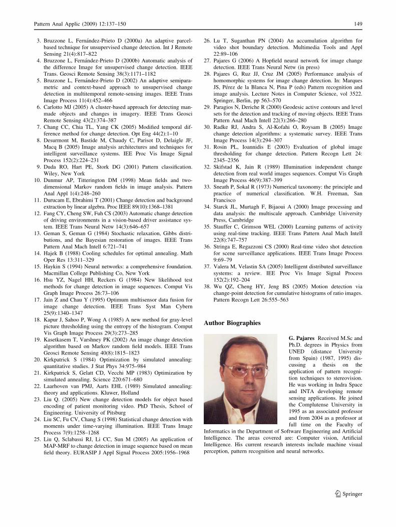
Author Biographies

G. Pajares Received M.Sc and

Ph.D. degrees in Physics from

UNED (distance University

from Spain) (1987, 1995) dis-

cussing a thesis on the

application of pattern recogni-

tion techniques to stereovision.

He was working in Indra Space

and INTA developing remote

sensing applications. He joined

the Complutense University in

1995 as an associated professor

and from 2004 as a professor at

full time on the Faculty of

Informatics in the Department of Software Engineering and Artificial

Intelligence. The areas covered are: Computer vision, Artificial

Intelligence. His current research interests include machine visual

perception, pattern recognition and neural networks.


123

Jose. J. Ruz received M.Sc

degree in Physics from the

Complutense University of

Madrid in 1974, and the Ph.D

degree in computer science in

1980 from the same University.

He joined the Department of

Computer Architecture and

Automatic Control of the Com-

plutense University in 1981

where he is a Professor. His

current research interest

includes parallel architectures

for distributed optimization,

high performance computing for pattern recognition and optimal path

planning for unmanned aerial vehicles.

J. M. de la Cruz received

M.Sc degree in Physics and

Ph.D. from the Complutense

University in 19790 and 1984,

respectively. From 1985 to 1990

he was with the Department of

Automatic Control, UNED

(Distance University of Spain),

and from October 1990 to 1992

with the Department of Elec-

tronic, University of Santander.

In October 1992, he joined the

Department of Computer Sci-

ence and Automatic Control of

the Complutense University where he is a Professor. His current

research interest includes robotics vision systems, fusion sensors and

applications of automatic control to robotics and flight control.


123

Image change detection from difference image through deterministic simulated annealing

Documents