ILO Projections of the Economically Active Population ... · 6 ILO Projections of the Economically Active Population – Revised Methodology of the 2011 Edition 2. Concepts, definitions

ILO Projections of the Economically Active Population

Revised Methodology of the 2011 Edition

Jean‐Michel Pasteels

April 2012

Copyright © International Labour Organization 2012 First published 2012 Publications of the International Labour Office enjoy copyright under Protocol 2 of the Universal Copyright Convention. Nevertheless, short excerpts from them may be reproduced without authorization, on condition that the source is indicated. For rights of reproduction or translation, application should be made to ILO Publications (Rights and Permissions), International Labour Office, CH‐1211 Geneva 22, Switzerland, or by email: [email protected]. The International Labour Office welcomes such applications. Libraries, institutions and other users registered with reproduction rights organizations may make copies in accordance with the licences issued to them for this purpose. Visit www.ifrro.org to find the reproduction rights organization in your country. ILO Cataloguing in Publication Data Pasteels, Jean Michel ILO projections of the economically active population: revised methodology of the 2011 edition / Jean‐Michel Pasteels ; International Labour Office, Department of Statistics. ‐ Geneva: ILO, 2012 1 v. (Working paper ; 4) ISBN: 9789221262213; 9789221262220 (web pdf) International Labour Office; Dept.of Statistics labour force participation / employment / labour force / measurement / projection / definition / methodology / role of ILO / developed countries / developing countries 13.01.2 The designations employed in ILO publications, which are in conformity with United Nations practice, and the presentation of material therein do not imply the expression of any opinion whatsoever on the part of the International Labour Office concerning the legal status of any country, area or territory or of its authorities, or concerning the delimitation of its frontiers. The responsibility for opinions expressed in signed articles, studies and other contributions rests solely with their authors, and publication does not constitute an endorsement by the International Labour Office of the opinions expressed in them. Reference to names of firms and commercial products and processes does not imply their endorsement by the International Labour Office, and any failure to mention a particular firm, commercial product or process is not a sign of disapproval. ILO publications and electronic products can be obtained through major booksellers or ILO local offices in many countries, or direct from ILO Publications, International Labour Office, CH‐1211 Geneva 22, Switzerland. Catalogues or lists of new publications are available free of charge from the above address, or by email: [email protected] Visit our web site: www.ilo.org/publns

Printed in Switzerland

ILO Projections of the Economically Active Population – Revised Methodology of the 2011 Edition 3

Contents

Preface .................................................................................................................................................................. 4

1. Introduction ...................................................................................................................................................... 5

2. Concepts, definitions and theoretical background .......................................................................................... 6

2.1. Measures of the Economically Active Population ............................................................................... 6

2.2. Different forms of employment .......................................................................................................... 6

2.3. Labour Force Participation Rates (LFPR) ............................................................................................. 6

2.4. The determinants of the LFPR ............................................................................................................. 7

3. Projection Methodologies used worldwide ..................................................................................................... 9

4. Methodology of the sixth edition .................................................................................................................. 11

4.1. Step 1 – Mechanic projections .......................................................................................................... 11

4.2. Step 2 – Combination of mechanic projections ................................................................................ 16

4.3. Step 3 – Judgmental adjustment ....................................................................................................... 17

4.4. Example of all steps ........................................................................................................................... 18

5. Strengths, limitations and directions for future work .................................................................................... 22

5.1. Strengths ........................................................................................................................................... 22

5.2. Limitations ......................................................................................................................................... 22

5.3. Direction for future work .................................................................................................................. 23

6. Bibliography ............................................................................................................................................. 24

Annex 1: Results from ex‐ante simulations ........................................................................................................ 25

Annex 2: Results from ex‐post simulations ........................................................................................................ 27

Annex 3: Data on international migrant stock ................................................................................................... 30

4 ILO Projections of the Economically Active Population – Revised Methodology of the 2011 Edition

Preface

The International Labour Office (ILO) programme on estimates and projections of the economically active population is part of a larger international effort on demographic estimates and projections to which several UN agencies contribute. Estimates and projections of the total population and its components by sex and age group are produced by the UN Population Division. Economically active population and its components by sex and age group are produced by the ILO, the agricultural population by the FAO and the school attending population by UNESCO.

The main objective of the ILO programme is to provide member States, international agencies and the public at large with the most comprehensive, detailed and comparable estimates and projections of the economically active population in the world and its main geographical regions. The first edition was published by the ILO Bureau of Statistics in 1971. The sixth edition was released in October 2011 (http://laborsta.ilo.org). It covers 191 countries and territories and the reference period for the estimates is 1990‐2010 and for the projections is 2011‐2020.

In this context, the Department of Statistics has decided to undertake a literature review of all the methodologies developed by national statistical offices and international organisations in order to derive projections of economically active population (Houriet‐Segard and Pasteels, 2011). This literature review was the starting point of the revision of the ILO methodology. This paper presents this revised methodology in detail.

The paper was prepared by Jean‐Michel Pasteels (ILO Department of Statistics) under the supervision of Rafael Diez de Medina, Director of the Department of Statistics. This work has benefited from the precious comments and inputs of Evangelia Bourmpoula, Mathieu Charpe, Stefanie Garry, Messaoud Hammouya, Geneviève Houriet‐Segard, Guy Mélard, Naima Pages and Dagmar Walter. Virginie Woest provided the secretarial support for the publication of the paper. Any remaining errors are the author’s sole responsibility.

Working papers of the Department of Statistics are meant to stimulate discussion. The ILO will therefore welcome comments and suggestions concerning the contents of this paper. They should be addressed to the Department of Statistics, International Labour Office, CH‐1211 Geneva 22, Switzerland, fax no. + 41 22 799 6957, e‐mail: [email protected].

Rafael Diez de Medina

Director

Department of Statistics

International Labour Office

April 2012


1. Introduction

The International Labour Office (ILO) programme on estimates and projections of the economically active population (EPEAP) is part of a larger international effort on demographic estimates and projections to which several UN agencies contribute. Estimates and projections of the total population and its components by sex and age group are produced by the UN Population Division, and employed populations by the ILO, the agricultural population by FAO and the school attending population by UNESCO.

The main objective of the ILO programme is to provide member States, international agencies and the public at large with the most comprehensive, detailed and comparable estimates and projections of the economically active population in the world and its main geographical regions. The first edition was published by the ILO Department of Statistics in 1971 (covering 168 countries and territories, with reference period 1950‐1985); the second edition in 1977 (with 154 countries and territories and reference period 1975‐2000); the third edition in 1986 (with 156 countries and territories and reference period 1985‐2025); the fourth edition in 1996 (with 178 countries and territories and reference period 1950‐2010); the fifth edition in 2007 (with 191 countries and reference period 1980‐2020) with two subsequent updates (in August 2008 and December 2009).

The sixth edition, released in October 2011, covers 191 countries and territories. The reference period for the estimates is 1990‐2010 and for the projections is 2011‐2020. For countries with historical data prior to 1990 (but after 1979), estimates concerning the period prior to 1990 are also provided.

The basic data are single‐year labour force participation rates by sex and age groups, of which ten groups are defined by five‐year age intervals (15‐19, 20‐24, ..., 60‐64) and the last age group is defined as 65 years and above. The data are available at the ILO main website for labour statistics: http://laborsta.ilo.org.

For the sixth edition, enhanced methodologies have been developed in order to improve the estimates and projections of the economically active population (EAP). In addition, detailed metadata are now provided, making the whole process more transparent than in the past and allowing the user to better use the information from the EAPEP database. The purpose of the present paper is to describe the new methodology adopted for the sixth edition for projecting the labour force participation rates (LFPR). Another paper (Bourmpoula et al. 2012) presents the changes in the methodology regarding the estimates of LFPR in detail.

Concerning the projection exercise, the projections are now based on a wider range of models than in the previous editions. Notably, they allow the capture of the impact of the latest (and still on‐going) economic crisis on the labour force participation for concerned countries. Finally, in this edition the ILO uses projections made by National Statistical Offices (NSOs), provided that these have been published recently.

The theoretical concepts are presented in section 2. The different methods used worldwide are briefly summarised in section 3. The new projection methodology is described in section 4. Finally, the strengths and limitations of the present methodology are presented in section 5, as well as proposed directions for future work.


2. Concepts, definitions and theoretical background

2.1. Measures of the Economically Active Population

As described in Hussmanns et al. (1990, p. 47), "the international standards identify two measures of the economically active population without excluding other possibilities: the usual active population measured in relation to a long reference period such as a year; and the currently active population, measured in relation to a short reference period such as one week or one day". The currently active population is the most widely measure of EAP and the term labour force is used synonymously. In this document, the terms EAP or labour force both refer to the currently active population.

2.2. Different forms of employment

The labour force is defined as the sum of the unemployed and the employed. For the exact definitions of those two concepts see Hussmanns et al. (1990). It is worth repeating the various forms of employment. The employed include people aged 15 and over who, during the reference week worked for one hour or more for pay, profit, commission or payment in kind, in a job or business or on a farm (comprising employees, employers and own account workers); or who worked for one hour or more without pay in a family business or on a family farm (i.e. contributing family workers); or who had a job, business or farm, but were not at work for various reasons (holiday, sickness, strike, etc..).

In brief, employment is of a dichotomous nature and covers people working a few hours per week, as well as those working a very large number of hours per week and cumulating several jobs. The employed can also be people engaged only in production of goods for own final use (subsistence work). In this regard, the international definition does not yet allow for the precise measurement of subsistence workers and there are large differences in terms of country practices regarding the treatment of this group in the labour force (see ILO 2011). Subsistence work can be extremely important in poor agrarian areas.

It is important to note that work in unpaid household services is not counted as employment, largely explaining differences in labour force participation rates by gender.

2.3. Labour Force Participation Rates (LFPR)

The labour force projections are obtained by the product of two separate projections: a projection of the population (POP) of country i at time t+h (t and h are respectively the projection origin and horizon) for the age group a (say the [20‐24]) and sex s, and a projection of the labour force participation rate (LFPR) for the same subgroup of the population.

sahtisahtisahti POPLFPRLF ,,,,,,,,, +++ ⋅=

where:sahti

sahtisahti POP

LFLFPR

,,,

,,,,,,

+

++ =

The LFPR are also used in the literature as activity rates or participation rates. The term labour force participation rate however, is more precise.

The decomposition of the projection exercise into two phases has several advantages. Firstly, the determinants of the changes in population and the LFPR are not the same and can be identified1. The determinants of the changes in population are primarily due to changes in fertility, mortality and migration flows (see United Nations 2011), while the changes in the LFPR can be the result of many factors, including

1 See Armstrong et al. (2005) for a presentation on the decomposition of complex time series and its pros and cons.


changes in labour demand, as highlighted in the next section. Secondly, the LFPR varies by definition between 0% and 100%, which is very convenient, since some logistic transformations can be applied to the LFPR in order to ensure that projected values within the 0‐100% interval are obtained.

It is important to highlight that the estimates and projections of the total population and its components by sex and age group are produced by the UN Population Division (UN 2011). The role of the ILO is to generate estimates and projections of LFPR that are consistent over time, across countries and across the various subgroups of the population of a given country.

2.4. The determinants of the LFPR

At the macroeconomic level, what is observed are average aggregated activity rates for the whole population or subgroups of it (male, female, prime age, youth, etc.). These data are derived from labour force or household surveys or from population censuses. As seen previously, the variable "participation rate" is of dichotomous nature: either you participate or you do not. The average number of hours the population is ready to work is not captured by macro‐economic data.

The determinants of the participation rate can be broken down into structural or long‐term factors, cyclical factors and accidental factors.

Structural factors include policy and legal determinants (e.g., flexibility of working‐time arrangements, taxation, family support, retirement schemes, apprenticeships, work permits, unemployment benefits, minimum wage) as well as other determinants (e.g., demographic and cultural factors, level of education, technological progress, availability of transportation).

Some key findings regarding female labour force participation rates (LFPR)2:

‐ In countries where working‐time arrangements are more flexible, there is a higher LFPR of female workers than in other countries.

‐ Taxation of second earners (relative to single earners) usually has a negative impact on female LFPR.

‐ Childcare subsidies and paid parental leave usually have a positive impact on female LFPR.

‐ In countries where the proportion of unmarried women is higher, there is usually a higher female LFPR than in other countries.

‐ Cultural factors such as strong family ties or religion have a strong impact on LFPR for some subgroups of the population. For example, in many countries, religious or social norms may discourage women from undertaking economic activities.

These structural factors are the main drivers of the long‐term patterns in the data. Changes in policy and legal determinants (e.g., changes in retirement and pre‐retirements schemes) can result in important shifts in participation rates from one year to another.

Cyclical factors refer to the overall economic and labour market conditions that influence the LFPR. In other words, demand for labour has an impact on the labour force. In times of strong slowdown or recession, two effects on the participation rates, with opposite signs, are referred to in the literature: the “discouraged worker effect” and the "additional worker effect”.

2 For more details see Jaumotte (2003).


The "discouraged worker effect" applies to persons not working but available for work, but who stopped to search for a job in the last four weeks. During times of recession, this effect is very important for younger people, who have usually more problems finding a job than more experienced workers. As noticed by the OECD (2010), in times of discouraging labour market conditions, the length of studies usually increases and the LFPR of younger age groups is more sensitive to severe downturns where there is easier access to post‐secondary education.

The "additional worker effect" applies more to female or older workers who enter (or re‐enter) the labour market in order to compensate for the job losses and decreased earnings of some members of the family or the community.

Also according to a recent OECD study (see OECD 2010), in times of severe downturns, the changes in the LFPR of older persons depend on financial incentives to continue working as compared to taking retirement.

Lastly, there are accidental factors such as wars, and natural disasters that also affect LFPR, usually in a temporary manner.


3. Projection Methodologies used worldwide

The ILO Department of Statistics recently undertook a literature review of all the EAP projection models used and developed by national statistical offices and international organizations (see Houriet‐Segard and Pasteels 2011). This document contains a description of the approach adopted by each national or international institution. A two page template has been used to describe the following aspects: the name of the institution, the frequency of updates and projection horizon, a brief description of the current methodology, the determinants that are captured explicitly, the use (or not) of scenarios, the assessment (or not) of the current methodology, the existence of any previous methodology, reference papers and additional comments. Some major findings of this literature review are presented in this section. To project LFPRs, four types of approaches have been identified in this document:

(A) Judgmental (or qualitative) methods based on scenarios or on the targets to be reached.

(B) Time extrapolation models or growth curves. Values for the measured variable can be expressed as a function of time and extrapolated over the projection period. There are many growth curves routinely used in the analysis of growth processes that ultimately reach a steady state. These generally form a class of s‐shaped or sigmoid curves, of which the most commonly used is the logistic curve. These sigmoid curves are very useful for modelling populations, labour force participation rates, inflation, productivity growth (not levels) or other processes where, in the long run, it is expected that the variable will not grow any further.

(C) Regression models based on correlations between participation rates and economic, demographic or cultural factors. A regression model with a set of explanatory variables is fitted on observed LFPRs. Future scenarios for the explanatory variables are determined and used in the regression model to project LFPRs. Regression models can be built at the country level (eg. France, UK) or for a group of countries (Asian Development Bank, European Commission) using panel regression techniques.

(D) Models based on a cohort approach. In this case, LFPRs are not projected by age and sex year after year, but they are projected from the estimated probability of entry or exit of the labour force for each age, sex and cohort (people born in a specific year). More specifically, the probability of entry and exit of the labour force are kept stable at the last observed value or are extrapolated over the projection period for each population cohort.

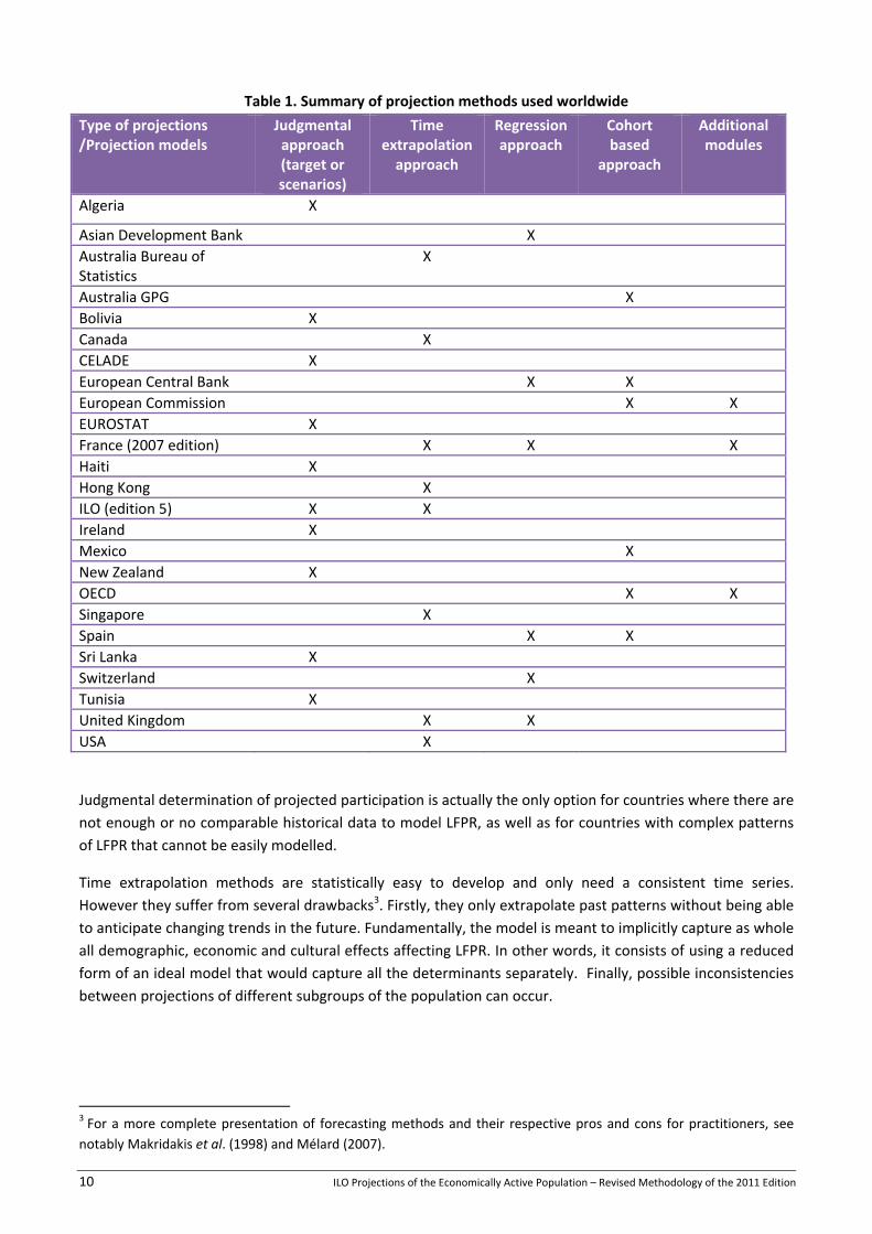
Table 1 lists the type(s) of methodology used by each national or international institution. It can be seen that judgmental and time extrapolation methods are the most frequently used. The main reason is of practical nature: these methods can be implemented more easily. The other approaches are more time‐consuming. Regression models are often statistically complex; they can be "heavy users" of historical and projected data. They rely on the accuracy of projected explanatory variables and the choice of the later can be a difficult and strategic process, for example when they change over time. Cohort based‐models need historical data over a long period to be implemented. Ideally, it should be pure longitudinal data (the same people surveyed year after year) but in fact, most of the projections are based on annual surveys based on different surveyed households. In addition, statistical procedures for projecting the cohorts' rates of entry or exit of the workforce quickly become complicated.


Table 1. Summary of projection methods used worldwide

Type of projections /Projection models

Judgmental approach (target or scenarios)

Time extrapolation approach

Regression approach

Cohort based

approach

Additional modules

Algeria X

Asian Development Bank X Australia Bureau of Statistics

X

Australia GPG X Bolivia X Canada X CELADE X European Central Bank X X European Commission X X EUROSTAT X France (2007 edition) X X X Haiti X Hong Kong X ILO (edition 5) X X Ireland X Mexico X New Zealand X OECD X X Singapore X Spain X X Sri Lanka X Switzerland X Tunisia X United Kingdom X X USA X

Judgmental determination of projected participation is actually the only option for countries where there are not enough or no comparable historical data to model LFPR, as well as for countries with complex patterns of LFPR that cannot be easily modelled.

Time extrapolation methods are statistically easy to develop and only need a consistent time series. However they suffer from several drawbacks3. Firstly, they only extrapolate past patterns without being able to anticipate changing trends in the future. Fundamentally, the model is meant to implicitly capture as whole all demographic, economic and cultural effects affecting LFPR. In other words, it consists of using a reduced form of an ideal model that would capture all the determinants separately. Finally, possible inconsistencies between projections of different subgroups of the population can occur.

3 For a more complete presentation of forecasting methods and their respective pros and cons for practitioners, see notably Makridakis et al. (1998) and Mélard (2007).


4. Methodology of the sixth edition

In this edition the ten years‐ahead projections are derived from a three steps procedure that uses both mechanic and judgmental approaches. The choice of a combination of mechanic and judgmental approach is justified by the review of the literature and the context: a large number of time series have to be modelled (more than 4'000) and the dataset contains many missing values (only 28 per cent of available records).

The first step consists of applying six mechanic models for each time series of LFPR for a given country, a given age group and gender. The reasons why these six mechanic models have been chosen are explained in the first section.

In the next step, the projections obtained from the six mechanic models are combined using a weighted average. The principle, with its pros and cons, of combining forecasts is presented in section 2 as well as the set of weights used for each subgroup of the population.

During the third phase, the combined projections are adjusted judgmentally in order to obtain consistent LFPR across gender and age groups for each. This aspect is critical as each time series is modelled independently. By construction there is no guarantee of consistency across gender and age groups. The third section explains the different criteria and rules of thumb that are applied.

The different steps of this methodology have been tested and implemented on the basis of ex‐ante and ex‐post experiments. Ex‐ante tests (before the action) consist of comparing the results obtained by this methodology with the projections published recently by NSOs. Ex‐post (after the action) experiments consist of dropping the last observations of a time series, then deriving projections on the basis of the shortened time series and calculating and analysing the ex‐post (also called "post‐sample") error projections. The results of these simulations are presented respectively in Annexes 1 and 2.

4.1. Step 1 – Mechanic projections

For each time series, several projections are derived from different model specifications (extrapolative and panel regressions), including a model specification that allows the capture of the impact of the latest economic crisis (still on‐going in some countries) on the labour force participation rate for concerned countries.

The different models that have been used are the following:

(1) Panel model used for deriving the estimates (weighted multivariate estimation)

(2) Pre‐crisis level of participation rate (average of 2006 and 2007)

(3) Transformed trend with a narrow range of asymptotes

(4) Transformed trend with a wide range of asymptotes

(5) Transformed trend with a wide range of asymptotes, estimated at more aggregated level (for a larger age‐group)

(6) Cyclical changes around a transformed trend (wider range of asymptotes)

Model 1 is the weighted multivariate estimation presented in section 2. Projections based on this model will notably be applied for countries for which it is already used to fill the missing historical data.


Models 2 to 5 are purely extrapolation methods (that use only historical data). Model 2 consists of the pre‐crisis LFPR (average of 2006 and 2007). It is a variant of a naive forecast (that the value for next year is expected to be the same as the previous year). It allows the capture of a scenario of return of LFPR to its pre‐crisis level on the forecasting horizon (2020 and before).

Models 3 to 5 are variant forms of the same basic model. The parametric form for the basic model is linear but fitted to the logistic transformation of the proportion participating, scaled to fit between the values ymin and ymax (the asymptotes) determined for each age‐sex group in a separate step. In this model, the participation rate yt at time t for the 22 subgroups of the population of each country are given by

btat eyy

yy +++=

1 -

minmaxmin

[1]

It can easily be demonstrated that the transformed variable y't , defined as minmax

min

- yy - yy y' t

t = [2], is equal

to the following expression: btat ey ++=′

11

[3]

Then, the transformed variable Y't, is defined as the logistic transformation of y't:

) )-y'/(( y' Y' ttt 1ln= [4]

It can also easily be shown that Y't = ‐ (a + bt). Consequently, the parameters a and b can be estimated by running a linear regression on Y't.

A special case is when ymin = 0 and ymax= 1 (the participation rates can vary between 0% and 100%). In this case, yt = y't and Y't corresponds to the same logistic transformation used in the estimation phase (see section 2).

This basic model was used in the previous edition of the projections (see ILO 2009). The way to define the asymptotes simply differs in this edition. It is a very convenient model, which combines the advantages of a logistic curve without suffering from its drawbacks.

The main advantage of the logistic curve and other sigmoid or S‐shaped curves is that they can capture growth processes that ultimately reach a steady state. These curves are frequently used for modelling populations and labour participation rates.

The S‐shaped curves, however, are not very easy to estimate. The logistic curve can be estimated using non‐linear least squares and maximum likelihood techniques. However, there are often problems in convergence and sometimes convergence cannot be achieved. In addition, imprecise estimates are obtained if the data does not clearly include an inflection point, i.e., the time at which the absolute value of the growth rate is maximised (for more details see Kshirsagar & Smith 1995). Estimating a logistic function on such data without imposing an assumption about when the inflection will occur will sometimes give nonsensical results. Figure 1 shows an example of unexpected projections of male LFPR obtained from a logistic curve.


Figure 1: Australia: Male LFPR (Age group: 35‐39). Projections based on growth curves vs real data

With this basic model, the method for defining the asymptotes is crucial. In the previous edition (see ILO 2009) the asymptotes were determined by looking jointly at the patterns of male and female participation rates for the same age group. The main assumption being that the past convergence or divergence between male and female LFPRs would continue in the future at the same pace as over the last ten years. This approach has been abandoned as it resulted in too many unexpected results (e.g., strong decreases in male LFPRs in the prime age, increased divergence between female and male LFPRs). More fundamentally, the assumption of continued joint divergence or convergence of male and female LFPRs is not fully justified theoretically, as many of the determinants of male and female LFPRs differ and the two rates may often move independently.

In this edition, it was decided to empirically test different alternative ways to set the asymptotes and to use the most appropriate set of asymptotes for each of the 22 subgroups of the population.

The simulation showed that working with two sets of asymptotes is enough: a narrow range of asymptotes where not much change is expected in the future and a wider one that allows larger changes in LFPR in the projection horizon. Figure 1 shows that the narrow range is well suited to male LFPR in the prime age. This is also confirmed by ex‐post simulations (see Annex 2). It is also worth mentioning that the two variants will give very close results when there is a flat trend.

80

82

84

86

88

90

92

94

96

98

100

Projection period

Original data

LINEAR (0‐100 asymptotes)

LINEAR (narrow asymptotes)

LOGISTIC (non‐linear procedure)


For each time series, the set of asymptotes are defined as follows:

ελ ⋅= -)min( min tyy [5]

ελ ⋅+= )max( max tyy [6]

Where λ is set to 1 for the narrow range of asymptotes and set to 1.5 for the wider range of asymptotes. The

value of ε represents the average absolute error of the naive method at the horizon of 10 years. It is calculated for each time series as follows:

n

yyt

ttt-t∑

+=

−=

1

0 1010

ε [7]

Where t0 is the first year and t1 the last year (n=t1‐t0). In other words, ε is a measure of volatility of the time series over ten year time intervals.

For countries with many data gaps, the value of ε is based on the sample of countries used to undertake the

ex‐post simulations (Annex 2). For example, for a sample of 22 countries, the value of ε is estimated at around 1 percentage point for male LFPR aged 30 and 49. This means that the LFPR is extremely stable over time and should not deviate more than 1 percentage point above its maximum past value and below its minimum past value in the next 10 years.

For female LFPR, values of ymin,f and ymax,f are also further adjusted (when necessary) in order to guarantee some consistency with the asymptotes estimated for male LFPR: ymin,m and ymax,m. More specifically, it consists of the following rules:

(i) setting ymin,f = ymin,m , if ymin,m <= ymin,f

(ii) setting ymax,f = ymax,m , if ymax,m <= ymax,f and yT,m > yT,f , where T represents the forecasting origin (2010 here).

The condition in the first rule is not met frequently but for the 15‐19 age group. The second rule states that if at the projection origin the male LFPR is higher than the female LFPR, then the asymptote for female LFPR should not exceed that for the male whatever the historical values.

Model 5 is similar to model 4 but what changes is simply the time series that is modelled. The principle is to undertake modelling for a larger subgroup of the population (eg. 25‐54), to derive projections at that level and to apply the growth rates of the projected aggregate for each 5‐year age band subgroup. By construction, the projections for each 5‐year age band will grow at the same pace. For male LFPR, the larger age bands are defined as [15‐24], [25‐54] and [55+]. For female LFPR, there are four larger age bands ([15‐24], [25‐39], [40‐54] and [55+]). The prime age group [25‐54] has been subdivided into two groups in order to take into account of the impact of maternity on LFPR.

Model 6 is a model that attempts to distinguish long‐term trends from short‐term changes due to changes in the business cycle. This approach has been adopted in a few countries. Notably, the NSO in the UK (see Madouros 2006 for more details), uses the following basic model:

⎟⎠

⎞⎜⎝

⎛= ∑

=−

n

kntttt yDUMMYTGAPf y

1),(,,, [8]


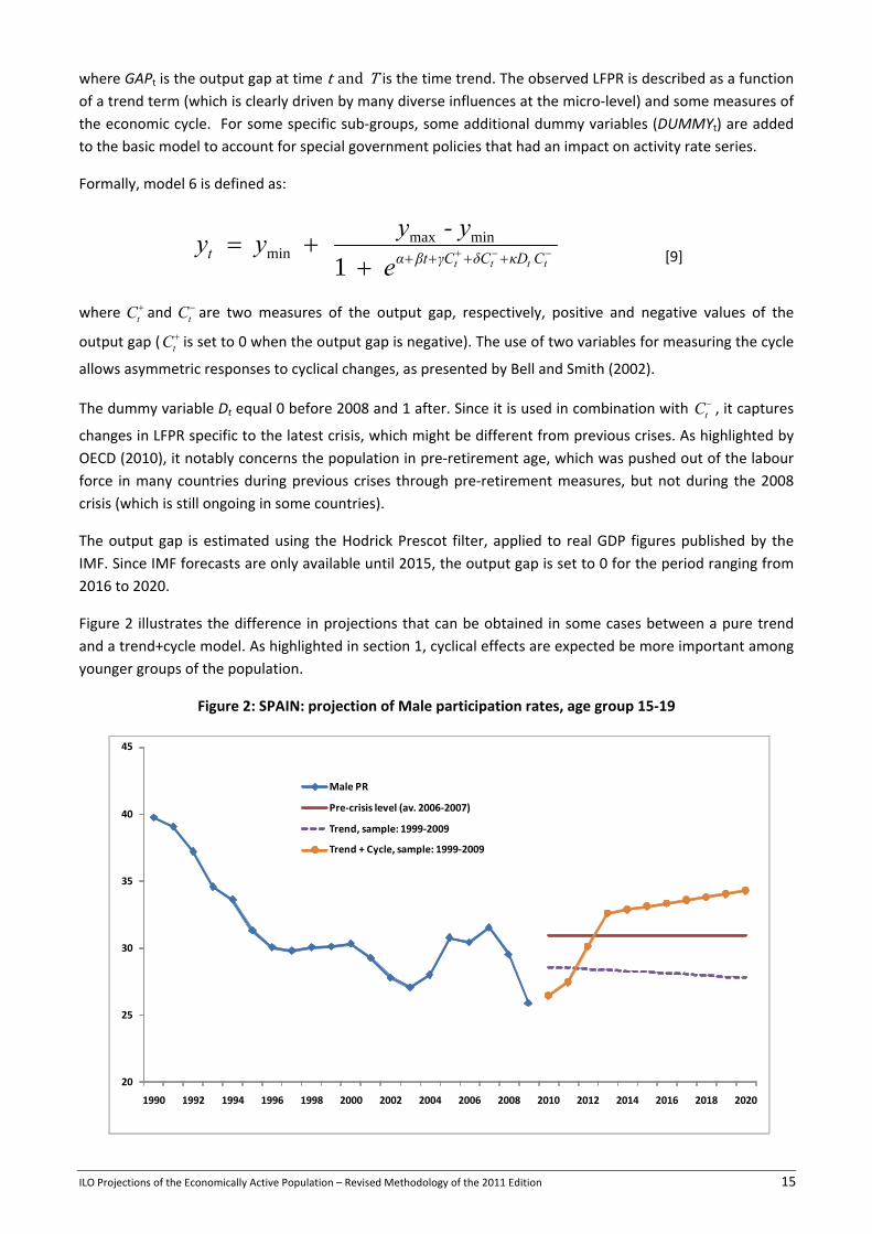
where GAPt is the output gap at time t and T is the time trend. The observed LFPR is described as a function of a trend term (which is clearly driven by many diverse influences at the micro‐level) and some measures of the economic cycle. For some specific sub‐groups, some additional dummy variables (DUMMYt) are added to the basic model to account for special government policies that had an impact on activity rate series.

Formally, model 6 is defined as:

−−+ ++++++=

tttt CκDδCγCβtαt e

- yy y y1

minmaxmin [9]

where +tC and −

tC are two measures of the output gap, respectively, positive and negative values of the

output gap ( +tC is set to 0 when the output gap is negative). The use of two variables for measuring the cycle

allows asymmetric responses to cyclical changes, as presented by Bell and Smith (2002).

The dummy variable Dt equal 0 before 2008 and 1 after. Since it is used in combination with −tC , it captures

changes in LFPR specific to the latest crisis, which might be different from previous crises. As highlighted by OECD (2010), it notably concerns the population in pre‐retirement age, which was pushed out of the labour force in many countries during previous crises through pre‐retirement measures, but not during the 2008 crisis (which is still ongoing in some countries).

The output gap is estimated using the Hodrick Prescot filter, applied to real GDP figures published by the IMF. Since IMF forecasts are only available until 2015, the output gap is set to 0 for the period ranging from 2016 to 2020.

Figure 2 illustrates the difference in projections that can be obtained in some cases between a pure trend and a trend+cycle model. As highlighted in section 1, cyclical effects are expected be more important among younger groups of the population.

Figure 2: SPAIN: projection of Male participation rates, age group 15‐19

20

25

30

35

40

45

1990 1992 1994 1996 1998 2000 2002 2004 2006 2008 2010 2012 2014 2016 2018 2020

Male PR

Pre‐crisis level (av. 2006‐2007)

Trend, sample: 1999‐2009

Trend + Cycle, sample: 1999‐2009


4.2. Step 2 – Combination of mechanic projections

The different projections are combined according to specific weights that have been calibrated on the basis of ex‐ante and ex‐post simulations.

Combining forecasts is an approach frequently used by forecast practitioners. Many empirical studies have been undertaken on the subject. Notably, see the reviews undertaken by Clemen (1989) and Armstrong (2001). As stated by Armstrong (2001), "Combining forecasts is especially useful when you are uncertain about the situation, uncertain about which method is most accurate, and when you want to avoid large errors. Compared with errors of the typical individual forecast, combining reduces errors".

It is also worth mentioning that there is a debate between practitioners and researchers. As summarised by Armstrong (2001), "Some researchers object to the use of combining. Statisticians object because combining plays havoc with traditional statistical procedures, such as calculations of statistical significance. Others object because they believe there is one right way to forecast. Another argument against combining is that developing a comprehensive model that incorporates all of the relevant information might be more effective.... Despite these objections, combining forecasts is an appealing approach. Instead of trying to choose the single best method, one frames the problem by asking which methods would help to improve accuracy, assuming that each has something to contribute. Many things affect the forecasts and these might be captured by using alternative approaches. Combining can reduce errors arising from faulty assumptions, bias, or mistakes in data."

The different empirical experiments also reveal that combining forecasts improves accuracy to the extent that the individual forecasts contain useful and independent information. Ideally, projection errors would be negatively related so that they might cancel each other out. In practice however, projections or forecasts are almost always positively correlated.

As illustrated in detail in Annex 2, the results from ex‐post simulations indicate non‐negligible gains in projection accuracy when combining projections. The gains are obvious for projections of male LFPR. However, for female LFPR, the tested combinations did not perform as well.

The weights used in this edition are based on the results from the ex‐ante and ex‐post experiments as well as two additional factors; the availability of historical data (at least 50% of historical records available for each time series) and the extent to which the country faced a recession or not since 2008.

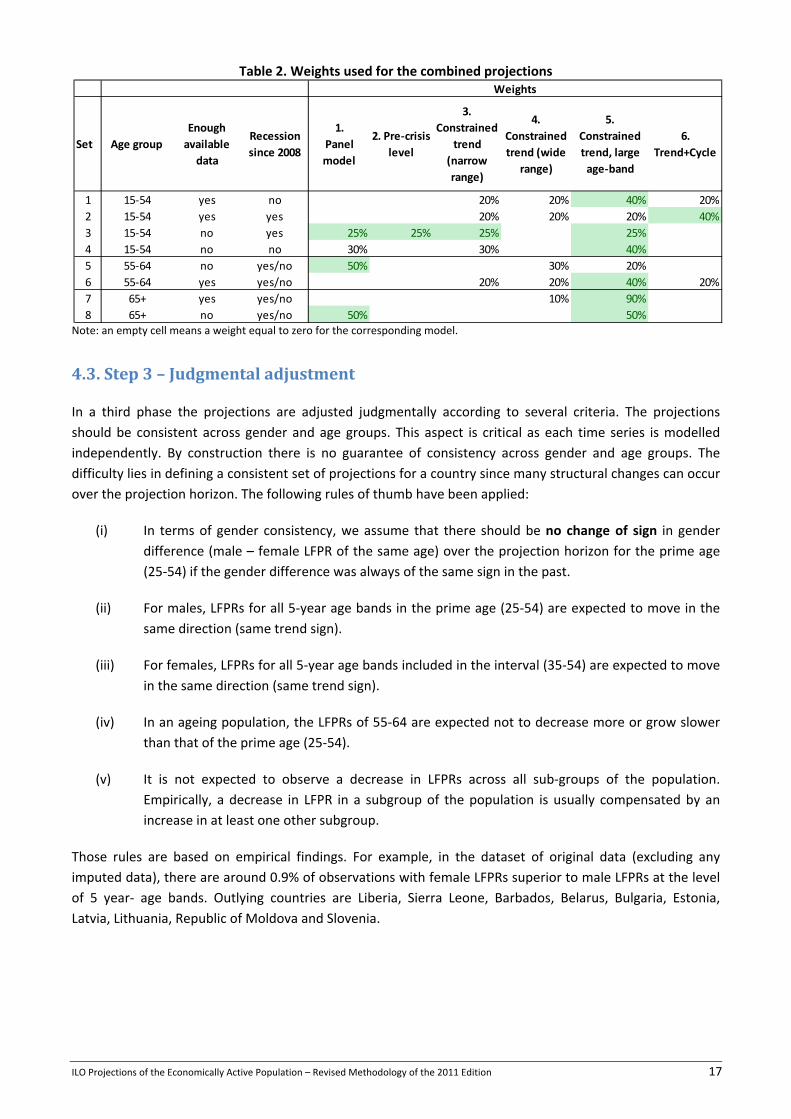
The weights are displayed in Table 2. In general, the highest weight is attributed to the constrained trend computed at the large age band level (model 5), which performed well during the simulations. When there are not enough observations, the "Trend+Cycle" model is not used, since there are not enough observations to perform a correct decomposition. For the sake of consistency, the panel model is used when there are not enough data, as this model is also used to fill the missing data.

The pre‐crisis level (a form of a naive method) is used in context of a recent recession in conjunction with a lack of a complete time series. Finally, for the 55‐64 and the 65+ age bands, the weights allocated to cyclical fluctuations are very low, since the determinants of a structural nature are more important in explaining changes in participation rates for this group of the population.


Table 2. Weights used for the combined projections

Note: an empty cell means a weight equal to zero for the corresponding model.

4.3. Step 3 – Judgmental adjustment

In a third phase the projections are adjusted judgmentally according to several criteria. The projections should be consistent across gender and age groups. This aspect is critical as each time series is modelled independently. By construction there is no guarantee of consistency across gender and age groups. The difficulty lies in defining a consistent set of projections for a country since many structural changes can occur over the projection horizon. The following rules of thumb have been applied:

(i) In terms of gender consistency, we assume that there should be no change of sign in gender difference (male – female LFPR of the same age) over the projection horizon for the prime age (25‐54) if the gender difference was always of the same sign in the past.

(ii) For males, LFPRs for all 5‐year age bands in the prime age (25‐54) are expected to move in the same direction (same trend sign).

(iii) For females, LFPRs for all 5‐year age bands included in the interval (35‐54) are expected to move in the same direction (same trend sign).

(iv) In an ageing population, the LFPRs of 55‐64 are expected not to decrease more or grow slower than that of the prime age (25‐54).

(v) It is not expected to observe a decrease in LFPRs across all sub‐groups of the population. Empirically, a decrease in LFPR in a subgroup of the population is usually compensated by an increase in at least one other subgroup.

Those rules are based on empirical findings. For example, in the dataset of original data (excluding any imputed data), there are around 0.9% of observations with female LFPRs superior to male LFPRs at the level of 5 year‐ age bands. Outlying countries are Liberia, Sierra Leone, Barbados, Belarus, Bulgaria, Estonia, Latvia, Lithuania, Republic of Moldova and Slovenia.

Set Age groupEnough available data

Recession since 2008

1. Panel model

2. Pre‐crisis level

3. Constrained

trend (narrow range)

4. Constrained trend (wide

range)

5. Constrained trend, large age‐band

6. Trend+Cycle

1 15‐54 yes no 20% 20% 40% 20%2 15‐54 yes yes 20% 20% 20% 40%3 15‐54 no yes 25% 25% 25% 25%4 15‐54 no no 30% 30% 40%5 55‐64 no yes/no 50% 30% 20%6 55‐64 yes yes/no 20% 20% 40% 20%7 65+ yes yes/no 10% 90%8 65+ no yes/no 50% 50%

Weights


The adjustments are also done on the basis of exogenous information such as:

a) Projected share of population aged 0‐14 and 55+ in total population and the projected share of female population in total population (Source: UN).

b) Forthcoming changes in retirement and pre‐retirement schemes and any other policy or legal determinants (National and international sources).

The information regarding projected population (a) is available for most countries. Concerning changes in forthcoming changes in retirement and pre‐retirement schemes and any other policy or legal determinants, some international sources that compile national information can be consulted4.

In the next section an adjustment based on (a) and (b) is illustrated.

Other types of information are also used in a less systematic way. These include the proportion of immigrant workers in the country and HIV prevalence. In this edition of the EAPEP database, the information was used primarily to check and manually adjust the estimated historical values. For example, in countries with high HIV prevalence, LFPR for all affected subgroups of the population (including male in the prime age) should be lower than in other countries. No specific adjustments of the projection horizon have been done on the basis of immigrant workers in the country and HIV prevalence.

For a dozen countries, the ILO uses projections made by National Statistical Offices, provided that these have been published recently. This concerns around twelve countries.

Linearization of projections between the projection origin and target

Once the final projections at the horizon 2020 are computed, the intermediate values from the projection origin (2010) and the target (2020) are filled assuming a linear pattern. This assumption may not be the most appropriate for all countries and groups of the population, especially when cyclical factors have a strong impact on the LFPR.

Nevertheless, it has been decided to apply this simple rule for the sake of consistency across all countries, in the absence of alternative solutions applicable to all time series.

This linear interpolation implies that users of the projections should have higher confidence in the participation rate projected at the horizon 2020 than in intermediate values.

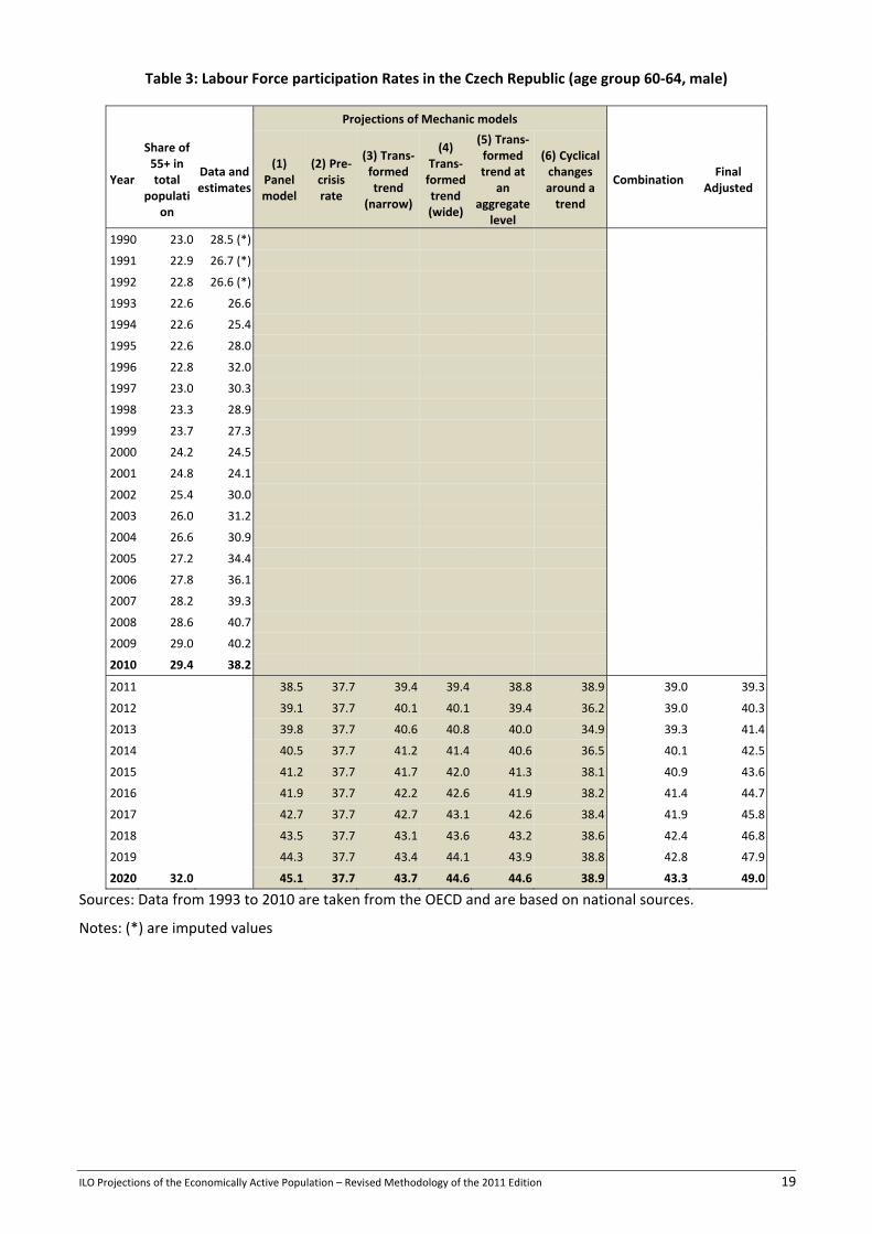
4.4 Example of all steps

The different steps used to derive projections are illustrated in this section. The time series under analysis is the male LFPR in the Czech Republic for the age group [60‐64]. In Table 3, all the computations used to derive the projections are presented.

4 The International Social Security Association (ISSA) provides detailed country profiles on social security schemes for almost all

countries in the world (see http://www.issa.int/Observatory/Country‐Profiles). The ILO Conditions of Work and Employment Branch provides information on maternity leaves, minimum wages and hours of work at http://www.ilo.org/dyn/travail/travmain.byCountry2. The OECD Family database (www.oecd.org/social/family/database) provides cross‐country information (only for OECD countries) on public policies for families and children (eg. Maternity leaves, childcare benefits, etc.).


Table 3: Labour Force participation Rates in the Czech Republic (age group 60‐64, male)

Projections of Mechanic models

Year

Share of 55+ in total

population

Data and estimates

(1) Panel model

(2) Pre‐crisis rate

(3) Trans‐formed trend

(narrow)

(4) Trans‐formed trend (wide)

(5) Trans‐formed trend at

an aggregate

level

(6) Cyclical changes around a trend

Combination Final

Adjusted

1990 23.0 28.5 (*)

1991 22.9 26.7 (*)

1992 22.8 26.6 (*)

1993 22.6 26.6

1994 22.6 25.4

1995 22.6 28.0

1996 22.8 32.0

1997 23.0 30.3

1998 23.3 28.9

1999 23.7 27.3

2000 24.2 24.5

2001 24.8 24.1

2002 25.4 30.0

2003 26.0 31.2

2004 26.6 30.9

2005 27.2 34.4

2006 27.8 36.1

2007 28.2 39.3

2008 28.6 40.7

2009 29.0 40.2

2010 29.4 38.2

2011 38.5 37.7 39.4 39.4 38.8 38.9 39.0 39.3

2012 39.1 37.7 40.1 40.1 39.4 36.2 39.0 40.3

2013 39.8 37.7 40.6 40.8 40.0 34.9 39.3 41.4

2014 40.5 37.7 41.2 41.4 40.6 36.5 40.1 42.5

2015 41.2 37.7 41.7 42.0 41.3 38.1 40.9 43.6

2016 41.9 37.7 42.2 42.6 41.9 38.2 41.4 44.7

2017 42.7 37.7 42.7 43.1 42.6 38.4 41.9 45.8

2018 43.5 37.7 43.1 43.6 43.2 38.6 42.4 46.8

2019 44.3 37.7 43.4 44.1 43.9 38.8 42.8 47.9

2020 32.0 45.1 37.7 43.7 44.6 44.6 38.9 43.3 49.0

Sources: Data from 1993 to 2010 are taken from the OECD and are based on national sources.

Notes: (*) are imputed values


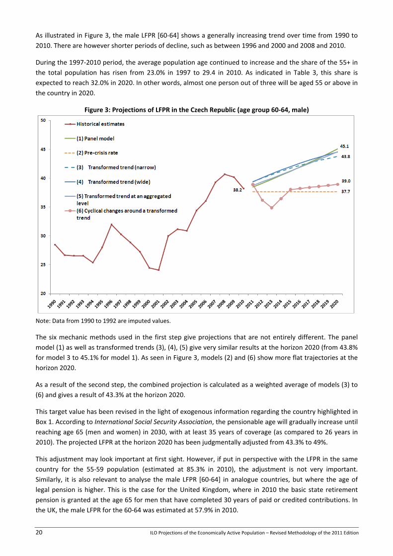
As illustrated in Figure 3, the male LFPR [60‐64] shows a generally increasing trend over time from 1990 to 2010. There are however shorter periods of decline, such as between 1996 and 2000 and 2008 and 2010.

During the 1997‐2010 period, the average population age continued to increase and the share of the 55+ in the total population has risen from 23.0% in 1997 to 29.4 in 2010. As indicated in Table 3, this share is expected to reach 32.0% in 2020. In other words, almost one person out of three will be aged 55 or above in the country in 2020.

Figure 3: Projections of LFPR in the Czech Republic (age group 60‐64, male)

Note: Data from 1990 to 1992 are imputed values.

The six mechanic methods used in the first step give projections that are not entirely different. The panel model (1) as well as transformed trends (3), (4), (5) give very similar results at the horizon 2020 (from 43.8% for model 3 to 45.1% for model 1). As seen in Figure 3, models (2) and (6) show more flat trajectories at the horizon 2020.

As a result of the second step, the combined projection is calculated as a weighted average of models (3) to (6) and gives a result of 43.3% at the horizon 2020.

This target value has been revised in the light of exogenous information regarding the country highlighted in Box 1. According to International Social Security Association, the pensionable age will gradually increase until reaching age 65 (men and women) in 2030, with at least 35 years of coverage (as compared to 26 years in 2010). The projected LFPR at the horizon 2020 has been judgmentally adjusted from 43.3% to 49%.

This adjustment may look important at first sight. However, if put in perspective with the LFPR in the same country for the 55‐59 population (estimated at 85.3% in 2010), the adjustment is not very important. Similarly, it is also relevant to analyse the male LFPR [60‐64] in analogue countries, but where the age of legal pension is higher. This is the case for the United Kingdom, where in 2010 the basic state retirement pension is granted at the age 65 for men that have completed 30 years of paid or credited contributions. In the UK, the male LFPR for the 60‐64 was estimated at 57.9% in 2010.


Box 1: Czech Republic: Qualitative information regarding the pension schemes

Old Age benefits:

Coverage: Employed and self‐employed persons, including students, unemployed persons, persons caring for children, needy persons, and military personnel.

Pensionable age :

• Old‐age pension: Age 62 and 2 months with at least 26 years of coverage (men); age 60 and 8 months with at least 26 years of coverage (women), or less according to the number of children reared; age 65 (men and women) with at least 15 years of coverage.

• Ongoing changes: The retirement age and required years of coverage are gradually increasing until reaching age 65 (men and women) in 2030, with at least 35 years of coverage.

Source: International Social Security Association, based on national sources.


5. Strengths, limitations and directions for future work

In this edition, the principle has been to increase transparency, to combine qualitative information and quantitative techniques and to exploit projections and other information published by NSOs. For the sake of continuous improvement, the strengths and weaknesses of this edition are described hereafter.

5.1. Strengths

(i) The data are more comparable across countries.

(ii) For the sake of transparency, the different mechanical projections (based on different assumptions) are provided in electronic format for users who would like to compare them and possibly select alternative assumptions.

(iii) Projections made by NSOs are used when available and published recently. These projections are expected to integrate more country‐specific expertise.

(iv) Consistency by gender and age group has been checked systematically.

5.2. Limitations

(a) The main limitation is that the tests and simulations (ex‐ante and ex‐post) are based on a limited sample of countries that may not be representative of all countries under analysis. This is a problem common to all calibration techniques (parameters are calibrated on a sub‐sample of countries). Unfortunately, forecasting simulations cannot be performed on countries lacking data or with time series with significant data gaps.

(b) By conception, any mechanic model has its shortcomings. Extrapolative models have a well‐known shortcoming; as described in the previous section.

(c) The "Trend + cycle" model sometimes resulted in unexpected results. This might be due to the use of annual data. The decomposition of a time series in trend and cycle components is usually suited to lower‐frequency data (quarterly or monthly data). Further work is needed in order to improve the "Trend + cycle" model.

(d) The judgmental adjustment described in the previous section may be too conservative in a few cases. In other words, they may under‐estimate changes in LFPR.

(e) The degree of confidence regarding the projections varies significantly across country. The confidence in the projections for one country depends primarily on the availability (and consistency) of historical data, that serve as a basis to derive the estimates. In this edition, no confidence intervals were published since the final estimates and projections are derived from various steps.

There are two extreme sets of countries: the ones for which historical data are available in a consistent manner over time (e.g., OECD countries) and those for which there is no consistent historical data at all5. It is advised to consider both estimates and projections derived for the later group as purely indicative.

5 The 17 countries or territories for which no comparable information on LFPR by sex and age exist to our knowledge are:

Afghanistan, Angola, Channel Islands, Eritrea, Guinea, Guinea‐Bissau, Democratic People's Republic of Korea, Libyan Arab Jamahiriya, Mauritania, Myanmar, Solomon Islands, Somalia, Swaziland, Turkmenistan, United States Virgin Islands, Uzbekistan, and Western Sahara.


Putting aside the criteria of availability of data, the projections of EAP are more uncertain for countries with high share of migrant workers, since migration flows are very difficult to predict.

5.3. Direction for future work

Future work should address each of the above mentioned limitations, bearing in mind the costs and benefits of each improvement.

In this edition, the weights used in order to derive the combined projection are the same for male and female LFPR. In the future, different sets of weights could be used by gender. The availability of more data points would help to refine the present set of weights.

For some of the 17 countries for which there is no data at all, micro‐datasets of third countries could be used as an alternative to econometric models (e.g., using micro‐data from some regions in Pakistan for estimating LFPR in Afghanistan). Also, LFPRs of one developing country can be projected to be the same as those of other more advanced countries or the same as actual rates in the more developed regions of the country under analysis.

The methodology could also be improved for countries with a high share of migrant workers or HIV prevalence.

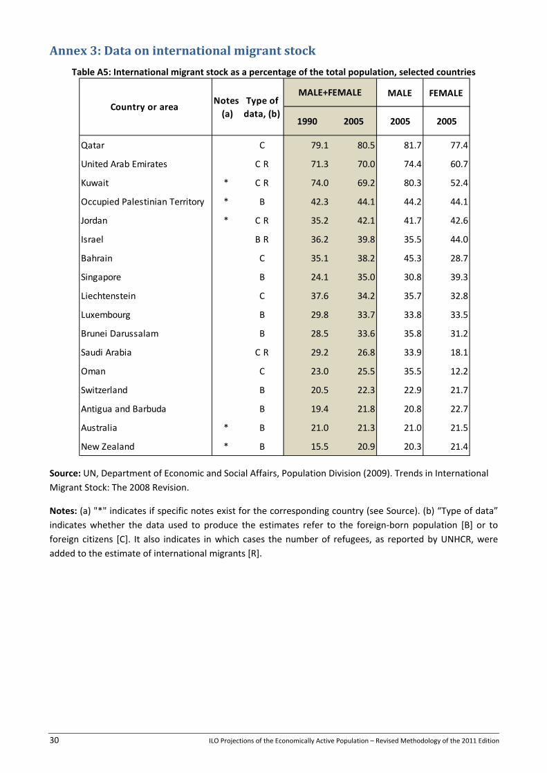
The table included in Annex 3 lists some of the countries with the highest shares of migrants. Cases in point include many countries from the Persian Gulf, such as Qatar and the United Arab Emirates, where share of migrants in the total population was estimated to exceed 70% in 2005 (United Nations 2009). In the methodology adopted by the Bank of Spain (see Cuadrado et al. 2007), the LFPRs for foreign residents are modelled separately. There are however different measurement and conceptual problems that reduce the international comparability of migration data6. The measurement problems are more important for countries where there are many seasonal migrants and migrants with contracts of a short duration, since they may be excluded from labour force surveys for practical reasons. In addition, this approach creates another issue: the need to obtain accurate projections of migration (stocks or flows) at the horizon 2020.

6 See notably Martí and Ródenas (2007) for an evaluation of the quality and cross‐country comparability of the statistical information

on migration derived from the EU Labour Force Surveys.


6. Bibliography

Armstrong J.S. (2001). Principles of Forecasting: A Handbook for Researchers and Practitioners. Armstrong (Ed.), Boston, Kluwer Academic Publishers.

Armstrong J.S, Collopy F., Yokum T. (2005). Decomposition by causal forces: a procedure for forecasting complex time series. International Journal of Forecasting 21 (2005) 25– 36.

Bourmpoula E., Kapsos S., Pasteels J.M. (2012). ILO Estimates of the Economically Active Population: 1990‐2010 (Sixth Edition). Employment Sector Working Paper Series. Forthcoming 2012.

Clemen, D. R. T. (1989). Combining forecasts: A review and annotated bibliography. International Journal of Forecasting, 5, 559‐583.

Cuadrado P., Lacuesta A., Martínez JM. and Pérez E. (2007). El futuro de la tasa de actividad española: un enfoque generacional. Documentos de Trabajo n° 0732, Banca de España, 63 p.

Houriet‐Segard G. and Pasteels J.M. (2011). Projections of Economically Active Population. A Review of National and International Methodologies. ILO Department of Statistics, Working Paper 3, December 2011.

Hussmanns R., Mehran F., Varmā V. (1990). Surveys of economically active population, employment, unemployment, and underemployment: An ILO manual on concepts and methods. International Labour Organization, Geneva.

ILO (2009). ILO Estimates and projections of the economically active population: 1980‐2020 (Fifth edition). Methodological description.

ILO (2011). Treatment of persons engaged in production of goods mainly for own final use. ILO Department of Statistics. Background document to the Second Meeting of the WG for the Advancement of Employment & Unemployment Statistics, Geneva, Switzerland (26‐28 October 2011).

Jaumotte J. (2003). Female labour force participation: past trends and main determinants in OECD countries. OECD Economics Department Working Papers, No. 376.

Kshirsagar A. M., Smith W.B. (1995). Growth curves. Dekker (Ed.), New York.

Madouros V. (2006). Labour Force Projections 2006‐2020. Office for National Statistics (UK), 39 p.

Makridakis S., Wheelwright S.C., Hyndman R.J. (1998). Forecasting: Methods and Applications. Wiley and Sons, New York, 3rd edition.

Martí M., Ródenas C. (2007). Migration Estimation Based on the Labour Force Survey: An EU‐15 Perspective. International Migration Review, vol. 41, pp. 101–126.

Mélard G. (2007). Méthodes de prévision à court terme. Ellipses, Paris, 2nd edition.

OECD (2010). The Impact of the Economic Crisis on Potential Output. Working Party No. 1 on Macroeconomic and Structural Policy Analysis ECO/CPE/WP1(2010)3. P.13.

United Nations (2009). Trends in International Migrant Stock: The 2008 Revision.

United Nations (2011). World Population Prospects: 2010 Revision Population Database.


Annex 1: Results from exante simulations

The exercise consists of comparing "ex‐ante" (before the action) projections from different models and to those made by National Statistics Organisations (NSO).

The twelve countries that are covered are displayed in the list below:

Country Source of projections (NSO) Australia Australian Government Productivity Group Austria STATISTICS AUSTRIA France INSEE Germany Institute for Employment Research (IAB) Hong Kong, China Hong Kong Statistics Office Ireland Central Statistics Office Mexico Conapo, Consejo Nacional de Poblacion Slovakia Demographic Research Centre, Infostat Sweden Statistiska centralbyrån Switzerland Office fédéral de la Statistique, Section Travail et vie active United Kingdom Office for National Statistics United States Bureau of Labor Statistics

The tables that follow display the average absolute discrepancy (expressed in percentage points of participation rate) between the projections published by the NSO and the projections obtained from each of the six models. The results are averaged over the twelve countries. For each line, the cell displaying the lowest value is in shaded. In other words, shaded cells highlight the method that gives the closest projections to that of the NSO.

It is worth mentioning that the most accurate method is unknown, since projections made by NSOs are also subject to prediction errors.

Table A1: Average absolute discrepancy for male LFPR

age group1.

Panel model


3. Constrained trend (narrow

range)


range)


6. Trend+Cycle

15‐19 3.5 2.8 2.7 3.1 3.9 3.720‐24 4.0 3.3 2.1 2.2 5.9 2.425‐29 0.8 1.1 0.9 1.0 1.4 1.330‐34 0.9 0.6 0.7 0.8 1.3 0.835‐39 0.5 0.7 0.6 0.6 1.2 0.840‐44 1.4 0.6 0.9 0.9 1.5 1.545‐49 1.2 0.7 1.0 1.1 1.3 1.450‐54 1.1 0.7 1.1 1.2 1.4 1.455‐59 2.2 3.6 2.1 2.3 7.4 2.360‐64 5.7 7.5 3.9 4.1 5.3 5.565+ 2.5 2.4 2.3 2.4 1.4 3.3


Table A2: Average absolute discrepancy for female LFPR

Age group

1. Panel model


3. Constrained trend (narrow

range)


range)


6. Trend+Cycle

15‐19 3.5 2.7 2.0 2.3 2.7 3.320‐24 3.7 3.0 2.6 2.7 5.0 3.925‐29 2.4 2.4 1.8 1.9 2.4 2.530‐34 2.6 4.2 2.0 2.3 2.1 2.835‐39 2.7 4.2 1.8 2.0 1.7 2.540‐44 2.1 3.6 1.2 1.5 1.2 1.745‐49 2.2 3.9 2.0 2.2 1.3 2.550‐54 3.1 5.5 2.1 2.4 1.2 2.655‐59 5.4 9.7 2.1 2.8 6.8 2.160‐64 3.7 9.4 3.7 4.2 3.3 4.465+ 1.1 2.0 1.2 1.1 0.8 1.6


Annex 2: Results from expost simulations

The principle of ex‐post (after the action) experiments consists of dropping the last observations of a time series, then deriving projections on the basis of the shortened time series and calculating and analysing the ex‐post (also called "post‐sample") error projections.

The sample includes 22 countries for which consistent historical data are available from 1985 to 2009. The countries include: Australia, Austria, Belgium, Canada, Costa Rica*, Denmark, Finland, France, Germany, Greece*, Hong Kong* (China), Ireland, Italy*, Japan, Korea Republic of*, Luxembourg, Norway, Portugal*, Spain*, Sweden, United Kingdom and United States. The seven countries that are followed by an "*" are part of a subsample of former developing and Southern European countries, for which the computations are presented separately.

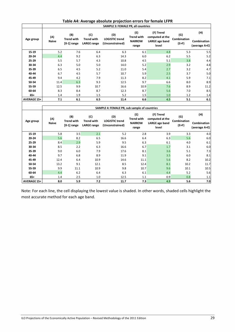
Tables A3 and A4 display the average absolute projection errors (expressed in percentage points of participation rate) at the horizon of ten years. The results are averaged over five projection exercises with the following projection origins: 1995, 1996, 1997, 1998 and 1999. For each line, the cell displaying the lowest value is shaded. In other words, shaded cells highlight the most accurate method for each age band.

The methods are not exactly the same as those tested during the ex‐ante experiment. The "Trend+Cycle" and the Panel Model could not have been replicated retroactively since they would needed old GDP and population forecasts made more than 15 years ago.

The main findings are the following:

(i) As expected, female LFPRs are more difficult to predict than male LFPRs. For both male and female LFPRs, the most delicate age bands to predict are seniors (55+) and young workers (15‐24).

(ii) In the prime age (25‐54), while female LFPRs are complex to project, male LFPRs display strong inertia over time. The naive method performs very well for male LFPRs in the prime age (25‐54), with an average absolute error of around 1 percentage point.

(iii) There are significant gains in accuracy when restrictions on the trends are added. In most cases, the linear trends with a constraint on the range (narrow or wide) perform better both than the linear trend (0‐1 range) and the logistic trend (non‐linear estimation).

(iv) In general, combining improves projection accuracy. The gains are obvious for projections of male LFPRs. For female LFPRs, the tested combinations did not perform as well.

(v) For female LFPRs, the constrained trend computed at the large age band level is in general the most accurate projection method. Except for the 20‐24 age groups, the naive method performs poorly for female LFPRs, since trends are more persistent than for male LFPRs.


Table A3: Average absolute projection errors for male LFPR

Note: For each line, the cell displaying the lowest value is shaded. In other words, shaded cells highlight the most accurate method for each age band.

SAMPLE 1: MALE PR, all countries

Age group(A)

Naive

(B) Trend with [0‐

1] range

(C) Trend with LARGE range

(D) LOGISTIC trend (Unconstrained)

(E) Trend withNARROW range

(F) Trend computed at the LARGE age band level

(G) Combination

(E+F)

(H)

Combination (average A+E)

15‐19 5.3 7.1 5.5 8.9 5.2 4.4 4.7 4.420‐24 4.6 10.6 5.5 8.6 5.1 6.0 4.8 4.325‐29 1.8 4.5 2.2 3.5 2.0 1.7 1.8 1.230‐34 1.2 3.8 1.5 1.9 1.4 1.2 1.2 0.935‐39 1.1 3.8 1.4 4.9 1.3 1.1 1.1 0.740‐44 1.1 4.6 1.3 2.9 1.3 1.1 1.1 1.045‐49 1.1 3.0 1.4 1.9 1.3 1.2 1.2 0.950‐54 1.9 4.4 2.9 3.2 2.8 2.4 2.5 1.655‐59 4.4 9.9 7.6 10.5 7.1 7.3 6.6 5.460‐64 6.6 12.3 10.6 16.1 9.8 7.7 8.6 7.965+ 2.4 3.2 3.0 7.1 2.9 2.1 2.4 2.3

AVERAGE 15+ 2.9 6.1 3.9 6.3 3.7 3.3 3.3 2.8

SAMPLE 2: MALE PR, sub sample of countries

Age group(A)

Naive

(B) Trend with [0‐

1] range




(F) Trend computed at the LARGE age band level

(G) Combination

(E+F)

(H)


15‐19 5.6 4.3 2.0 6.2 2.5 2.9 2.6 3.820‐24 7.6 11.8 5.7 10.0 5.7 6.5 5.3 6.425‐29 2.9 6.7 2.6 10.5 2.5 2.5 2.4 2.530‐34 1.7 3.3 1.8 1.5 1.8 1.1 1.4 1.635‐39 1.2 1.2 1.0 4.2 1.0 0.5 0.6 1.140‐44 1.3 1.2 1.3 1.5 1.3 0.6 0.8 1.345‐49 1.0 2.1 1.6 0.7 1.5 1.0 1.1 1.250‐54 2.6 5.4 3.4 4.4 3.2 2.8 2.8 2.855‐59 2.7 6.9 5.3 4.3 4.9 9.8 6.9 3.560‐64 3.1 8.2 6.1 9.3 5.2 6.9 5.9 3.365+ 2.1 2.7 2.1 5.5 2.1 1.3 1.7 2.1

AVERAGE 15+ 2.9 4.9 3.0 5.3 2.9 3.3 2.9 2.7


Table A4: Average absolute projection errors for female LFPR

Note: For each line, the cell displaying the lowest value is shaded. In other words, shaded cells highlight the most accurate method for each age band.

SAMPLE 3: FEMALE PR, all countries

Age group(A)

Naive

(B) Trend with [0‐1] range




(F) Trend computed at the LARGE age band

level

(G) Combination

(E+F)

(H)


15‐19 5.2 7.6 6.4 6.3 6.1 4.8 5.3 5.520‐24 4.4 9.2 6.3 14.3 6.0 6.2 5.5 5.225‐29 5.5 5.7 4.3 10.8 4.5 5.1 3.8 4.430‐34 6.3 5.0 5.0 14.0 5.2 2.9 3.2 4.835‐39 6.5 4.5 5.2 11.0 5.4 2.7 3.2 4.740‐44 6.7 4.5 5.7 10.7 5.9 2.5 3.7 5.045‐49 9.4 4.2 7.9 11.3 8.2 4.1 5.9 7.150‐54 11.4 6.3 9.3 12.5 9.7 6.6 8.0 8.955‐59 12.5 9.9 10.7 16.6 10.9 7.6 8.9 11.260‐64 8.3 8.4 8.7 12.3 8.7 5.6 7.0 8.565+ 1.4 1.9 1.5 5.2 1.5 1.0 1.2 1.4

AVERAGE 15+ 7.1 6.1 6.5 11.4 6.6 4.5 5.1 6.1

SAMPLE 4: FEMALE PR, sub sample of countries

Age group(A)

Naive

(B) Trend with [0‐1] range




(F) Trend computed at the LARGE age band

level

(G) Combination

(E+F)

(H)


15‐19 5.8 3.5 2.1 5.2 2.8 3.9 3.3 4.020‐24 5.6 8.2 6.5 16.6 6.4 6.3 5.6 6.025‐29 8.4 2.9 5.9 9.5 6.3 6.1 4.0 6.130‐34 8.5 2.2 6.3 16.6 6.7 1.7 3.1 6.035‐39 9.0 6.0 7.9 17.6 8.1 3.6 5.1 7.340‐44 9.7 6.8 8.9 11.9 9.1 3.5 6.0 8.145‐49 12.4 6.4 10.9 14.6 11.1 5.6 8.2 10.250‐54 13.2 9.1 12.1 8.5 12.4 8.1 10.2 11.755‐59 9.9 11.1 10.9 9.8 10.7 9.6 10.1 10.560‐64 4.4 6.2 6.4 6.3 6.1 4.4 5.2 5.665+ 1.4 2.5 1.0 12.5 1.1 0.9 0.8 1.1

AVERAGE 15+ 8.0 5.9 7.2 11.7 7.3 4.9 5.6 7.0


Annex 3: Data on international migrant stock

Table A5: International migrant stock as a percentage of the total population, selected countries

Source: UN, Department of Economic and Social Affairs, Population Division (2009). Trends in International Migrant Stock: The 2008 Revision.

Notes: (a) "*" indicates if specific notes exist for the corresponding country (see Source). (b) “Type of data” indicates whether the data used to produce the estimates refer to the foreign‐born population [B] or to foreign citizens [C]. It also indicates in which cases the number of refugees, as reported by UNHCR, were added to the estimate of international migrants [R].

MALE FEMALE

1990 2005 2005 2005

Qatar C 79.1 80.5 81.7 77.4

United Arab Emirates C R 71.3 70.0 74.4 60.7

Kuwait * C R 74.0 69.2 80.3 52.4

Occupied Palestinian Territory * B 42.3 44.1 44.2 44.1

Jordan * C R 35.2 42.1 41.7 42.6

Israel B R 36.2 39.8 35.5 44.0

Bahrain C 35.1 38.2 45.3 28.7

Singapore B 24.1 35.0 30.8 39.3

Liechtenstein C 37.6 34.2 35.7 32.8

Luxembourg B 29.8 33.7 33.8 33.5

Brunei Darussalam B 28.5 33.6 35.8 31.2

Saudi Arabia C R 29.2 26.8 33.9 18.1

Oman C 23.0 25.5 35.5 12.2

Switzerland B 20.5 22.3 22.9 21.7

Antigua and Barbuda B 19.4 21.8 20.8 22.7

Australia * B 21.0 21.3 21.0 21.5

New Zealand * B 15.5 20.9 20.3 21.4

MALE+FEMALE

Country or area Notes (a)

Type of data, (b)

ILO Projections of the Economically Active Population ... · 6 ILO Projections of the Economically Active Population – Revised Methodology of the 2011 Edition 2. Concepts, definitions

Documents