Ill-posed inverse problems in economics - Cemmap · posed inverse problem. problems arise in many settings in economics and other fields Such problems arise in many settings in economics

Ill-posed inverse problems in economics

Joel Horowitz

The Institute for Fiscal Studies Department of Economics, UCL

cemmap working paper CWP37/13

ILL-POSED INVERSE PROBLEMS IN ECONOMICS

by

Joel L. Horowitz Department of Economics Northwestern University

Evanston, IL 60208 [email protected]

August 2013

ABSTRACT

A parameter of an econometric model is identified if there is a one-to-one or many-to-one mapping from the population distribution of the available data to the parameter. Often, this mapping is obtained by inverting a mapping from the parameter to the population distribution. If the inverse mapping is discontinuous, then estimation of the parameter usually presents an ill-posed inverse problem. Such problems arise in many settings in economics and other fields where the parameter of interest is a function. This paper explains how ill-posedness arises and why it causes problems for estimation. The need to modify or “regularize” the identifying mapping is explained, and methods for regularization and estimation are discussed. Methods for forming confidence intervals and testing hypotheses are summarized. It is shown that a hypothesis test can be more “precise” in a certain sense than an estimator. An empirical example illustrates estimation in an ill-posed setting in economics. Keywords: regularization, nonparametric estimation, density estimation, deconvolution, nonparametric instrumental variables, Fredholm equation I thank Joachim Freyberger and Chuck Manski for very helpful comments on a previous draft of this paper.

2

TABLE OF CONTENTS

1. INTRODUCTION 1

2. MOTIVATING EXAMPLES 4

2.1 Examples of Continuous and Discontinuous Identifying Relations 4

2.2 The Control Function Model 11

3. EXAMPLES FROM OTHER FIELDS 13

3.1 Computerized Tomography and the Radon Transformation 13

3.2 Restoration of a Distorted and Noisy Image 16

4. REGULARIZATION AND ESTIMATION OF MODELS WITH ILL-POSED

INVERSES 18

4.1 Nonparametric Density Estimation 18

4.2 Deconvolution 21

4.3 Nonparametric IV Estimation 23

4.4 The Difference between Parametric and Nonparametric IV Estimation 29

5. INFERENCE 30

5.1 Confidence Regions 31

5.2 Hypothesis Tests 37

6. AN EMPIRICAL ILLUSTRATION 41

7. CONCLUSIONS 43

8. APPENDIX 44

8.1 An Example that Illustrates the Discontinuity of the Inverse of Mapping (15) 44

8.2 Procedure for Regularizing and Estimating g in Model (13) 45

REFERENCES 50

1

ILL-POSED INVERSE PROBLEMS IN ECONOMICS

1. INTRODUCTION

A parameter of an econometric model is said to be identified if it is uniquely determined

by the probability distribution from which the available data are sampled (hereinafter the

population distribution). In other words, a parameter is identified if there is a one-to-one or

many-to-one mapping from the population distribution to the parameter. The parameter may be

a scalar, vector, or function. In many familiar economic settings, such as least squares (LS) or

instrumental variables (IV) estimation of a linear model, the parameter of interest is a scalar or

vector, and the identifying mapping is continuous. That is, small changes in the population

distribution of the data produce only small changes in the identified parameter. When this

happens, the parameter of interest can be estimated consistently by replacing the unknown

population distribution with a consistent sample analog, such as the empirical distribution of the

data (Manski 1988). Consistency of the sample analog implies that the difference between the

sample analog and true population distribution is small when the sample size is large. The

estimated parameter is consistent for the true parameter because continuity of the identifying

mapping implies that the difference between the estimated and true parameter values is small if

the difference between the sample analog and true population distribution is small.

This approach to estimation does not necessarily work if the mapping that identifies the

parameter of interest is discontinuous. Nonparametric IV estimation and deconvolution are

examples of discontinuous mappings in economics in which the parameter of interest cannot be

estimated consistently by replacing the unknown population distribution with a consistent sample

analog. Nonparametric IV estimation is a generalization of conventional IV estimation of a

linear model. Deconvolution and closely related estimation problems are important in models

2

with errors in variables (Chen, Hong, and Nekipilov 2011; Li 2002; Li and Hsiao 2004;

Schennach 2004a; Schennach 2004b), panel-data models (Horowitz and Markatou 1996), models

with latent factors (Bonhomme and Robin 2010), empirical models of auctions (Li, Perrigne, and

Vuong 2000), and estimation using aggregated data (Linton and Whang 2002). Many other

examples of discontinuous mappings arise in mathematics, statistics, and engineering. Some of

these are described in Section 3 of this paper. Others are described by O’Sullivan (1986) and

Engl, Hanke, and Neubauer (1996). In each case, the parameter of interest cannot be estimated

consistently by replacing the population distribution of the data with a consistent sample analog

in the identifying mapping. This is because the estimated and true values of the parameter may

be very different, even if the sample size is large enough to make the difference between the

sample analog and population distribution negligibly small.

An estimation problem is called ill posed if the identifying mapping is discontinuous in a

way that prevents consistent estimation of the parameter of interest by replacing the population

distribution of the data with a consistent sample analog. The problem is called an ill-posed

inverse problem if the discontinuous identifying mapping is obtained by inverting another

mapping that is continuous. The concept of ill-posedness is usually attributed to Hadamard

(1923), who called a problem well-posed if it has a unique solution that depends continuously on

the available data. An ill-posed problem is one that is not well-posed. This concept can be

formalized (e.g., Kress (1999, Definition 15.1)), but formalization is not needed for the

discussion in this paper. In the context of this paper, the uniqueness condition for well-

posedness is equivalent to identification of the parameter of interest. The continuity condition

means that replacing the population distribution of the data with a consistent sample analog in

the identifying mapping yields a consistent estimator of the parameter. The concept of ill-

3

posedness differs from non-robustness (Huber 1981). Non-robustness refers to a situation in

which the population distribution of the data differs from the one assumed in a model. Ill-

posedness refers to a type of estimation problem that arises in a correct model.

This paper shows how ill-posed inverse problems arise, explains how estimation and

inference can be carried out in ill-posed settings, and explains why estimation in these settings is

important in economics. The paper focusses on three examples that illustrate the issues and

methods associated with ill-posed inverse problems. These are nonparametric estimation of a

probability density function, deconvolution density estimation, and nonparametric IV estimation.

The remainder of the paper is organized as follows. Section 2 provides examples of

continuous and discontinuous identifying mappings. These illustrate how discontinuity can arise

in problems that are important in economics. Section 2 also explains why discontinuity causes

problems for estimation and inference. Section 3 presents examples of ill-posed inverse

problems in mathematics, statistics, and engineering. The econometrics literature on ill-posed

inverse problems builds on research in these fields, some of which is over 100 years old and very

important in modern medicine and image processing. Section 4 treats regularization and

estimation of models that present ill-posed inverse problems. The term “regularization” refers to

methods for removing the discontinuity in the identifying mapping in order to facilitate

estimation. Different models and estimation problems require different regularization methods

depending, especially, on the source of discontinuity in the identifying mapping. Section 4

discusses regularization and estimation of the models described in Section 2. Section 5 discusses

confidence intervals and hypothesis tests based on these models. Section 6 presents an empirical

example that illustrates estimation in an ill-posed setting in economics. Section 7 presents

concluding comments. Section 8 is an appendix that presents technical material that is not

4

essential for understanding the main ideas of the paper. Unless otherwise stated, it is assumed

throughout this paper that all random variables are continuously distributed.

2. MOTIVATING EXAMPLES

This section provides examples that illustrate the difference between continuous and

discontinuous identifying mappings and how a discontinuous mapping can arise in settings that

are important in economics. The examples help to motivate the discussion in Sections 4 and 5 of

estimation and inference in ill-posed problems.

2.1. Examples of Continuous and Discontinuous Identifying Relations

The first example of a continuous mapping is the identifying relation of the familiar

linear mean-regression model. The model is

(1) ; ( | ) 0Y X U E U Xβ= + = ,

where Y is the scalar-valued dependent variable, X is a 1 p× vector of explanatory variables,

U is an unobserved, scalar random variable, and β is a 1p× vector of constants. Let jX

denote the j ’th component of X . Assume that 2( )E Y M≤ and 2( )jE X M≤ for each

1,...,j p= and some constant M < ∞ . Equation (1) implies that

(2) ( ) [ ( )]E X Y E X X β′ ′= .

Inversion of (2) yields the relation

(3) 1[ ( )] ( )E X X E X Yβ −′ ′= .

Equation (3) determines β uniquely if ( )E X X′ is a non-singular matrix. Thus, (3) identifies β .

Moreover β is a continuous function of ( )E X X′ , ( )E X Y′ , and the probability distribution of

( , )Y X . Small changes in these quantities cause only small changes in β .

5

Another example of a continuous mapping is obtained by allowing X to be endogenous

but assuming that an instrumental variable Z is available. Model (1) then becomes

(4) ; ( | ) 0Y X U E U Zβ= + = ,

where Z is a 1 q× vector and q p≥ . As before, assume that 2( )E Y M≤ and 2( )jE X M≤ for

some constant M < ∞ . Also assume that each component jZ of Z satisfies 2( )jE Z M≤ .

Equation (4) implies that

( ) [ ( )]E Z Y E Z X β′ ′=

and, therefore,

(5) 1 1( )[ ( )] ( ) ( )[ ( )] [ ( )]E X Z E Z Z E Z Y E X Z E Z Z E Z X β− −′ ′ ′ ′ ′ ′=

Inversion of (5) yields

(6) 1 1 1{ ( )[ ( )] ( )} ( )[ ( )] ( )E X Z E Z Z E Z X E X Z E Z Z E Z Yβ − − −′ ′ ′ ′ ′ ′= .

The parameter β is uniquely determined if the inverse matrices on the right-hand side of (6)

exist. Thus, (6) identifies β in model (4). Moreover, β is a continuous function of the

moments and the probability distributions of the random variables on the right-hand side of (6).

Now consider estimation of β in models (1) and (4). Suppose the data available for

estimating β in (1) are a random sample from the probability distribution of ( , )Y X . Then β in

(1) can be estimated by replacing the unknown population expectations in (3) with sample

averages. This is equivalent to replacing the unknown distribution of ( , )Y X with the empirical

distribution of the data. Denote the data by { , : 1,..., }i iY X i n= . Define the sample averages

1

1

n

XY i ii

m n X Y−

=

′= ∑

and

6

1

1

n

XX i ii

m n X X−

=

′= ∑ .

Then β in model (1) is estimated by replacing ( )E X Y′ with XYm and ( )E X X′ with XXm in (3)

to obtain the ordinary least squares estimator

1ˆLS XX XYm mβ −= .

Now suppose the data for estimating β in (4) are a random sample from the probability

distribution of ( , , )Y X Z . Then β in model (4) can be estimated by replacing the unknown

population expectations in (6) with sample averages. Denote the data by { , , : 1,..., }i i iY X Z i n= .

Define the sample averages

1

1

n

ZY i ii

m n Z Y−

=

′= ∑ ,

1

1

n

ZZ i ii

m n Z Z−

=

′= ∑

and

1

1

n

ZX i ii

m n Z X−

=

′= ∑ .

Then replacing ( )E X Z′ , ( )E Z Z′ , and ( )E Z Y′ , respectively, with XZm , ZZm , and ZYm in (6)

yields the two-stage least squares estimator

1 1 1ˆ ( )IV XZ ZZ XZ XZ ZZ ZYm m m m m mβ − − −′ ′= .

The estimators ˆLSβ and ˆ

IVβ are consistent for β in their respective models. This is

because (1) the sample averages entering ˆLSβ and ˆ

IVβ are consistent for their corresponding

population moments and (2) the identifying relations (3) and (6) are continuous functions of the

7

population expectations on their right-hand sides. Consistency of the sample averages implies

that they are arbitrarily close to the corresponding population moments when n is sufficiently

large. Consistency combined with continuity of (3) and (6) implies that ˆLSβ and ˆ

IVβ are

arbitrarily close to β when n is sufficiently large.

As was discussed in Section 1, however, there are important settings in which the relation

that identifies a parameter is discontinuous. Discontinuous identifying relations often arise when

the parameter of interest is a function, rather than a finite-dimensional quantity. An example is

the relation that identifies the probability density function of a scalar, continuously distributed

random variable in terms of that variable’s cumulative distribution function. The relation is

(7) ( )( ) dF xf xdx

= ,

where f is the probability density function and F is the cumulative distribution function. The

mapping (7) from F to f is discontinuous. Equation (7) is the inverse of

(8) ( ) ( ) ( )F x I v x f v dv∞

−∞= ≤∫ ,

where ( )I ⋅ is the indicator function. Equation (8) is a continuous mapping, but (7) is not. In (8),

small changes in f can induce only small changes in F , but the converse is not true.

Arbitrarily small changes in F can induce large changes in f . To see this, suppose that

( )f x a≤ for some a < ∞ . Then F can be approximated arbitrarily well uniformly in x by a

step function. Given any 0ε > , there is a step function, StepF , such that

(9) sup | ( ) ( ) |Stepx

F x F x ε−∞< <∞

− < .

Define

( ) ( ) /Step Stepf x dF x dx= .

8

Then ( )Stepf x = ∞ at jumps of StepF , and ( ) 0Stepf x = elsewhere. Therefore, | ( ) ( ) |Stepf x f x−

can be arbitrarily large, even if | ( ) ( ) |StepF x F x− is arbitrarily small. Accordingly, estimation of

f in (7) (nonparametric density estimation) is an ill-posed inverse problem. The probability

density function f cannot be estimated consistently by replacing F on the right-hand side of (7)

by the empirical distribution function

1

1( ) ( )

n

n ii

F x n I X x−

=

= ≤∑ .

Although nF is a uniformly consistent estimator of F , it is a step function. Its derivative is

always 0 or ∞ and never approaches ( )f x when 0 ( )f x< < ∞ , regardless of how large n is.

Deconvolution provides a second example of an ill-posed inverse problem that is

important in economics. The source of the problem is illustrated by a simple, idealized model of

measurement error. More realistic versions of deconvolution are described by Horowitz and

Markatou 2006); Delaigle, Hall, and Meister (2008); Johannes (2009); Li (2002); Li, Perrigne,

and Vuong (2000); Schennach (2004a, 2004b); and Linton and Whang (2002), among many

others. Suppose one wants to know the distribution of a continuously distributed random

variable X that is measured with error. X is not observed. Rather, one observes the random

variable Y that is related to X by

(10) ; ~ (0,1)Y X Nε ε= + .

The data, { : 1,..., }iY i n= are a random sample of Y . Let Yf and Xf , respectively, denote the

probability density functions of Y and X . Let φ denote the standard normal probability density

function. Then Yf is identified by the sampling process, can be estimated by nonparametric

density estimation, and is related to Xf , the density of interest, by

9

(11) ( ) ( ) ( )Y Xf y f v y v dvφ∞

−∞= −∫ .

Thus, Yf is the convolution of Xf and φ . The density Xf is identified as the solution to the

integral equation (11) (thus, the term “deconvolution”). The solution to (11) and the mapping

that identifies Xf is

(12) 2 /21( ) ( )

2itx t

X Yf x e h t dtπ

∞ − +−∞

= ∫ ,

where Yh is the characteristic function of the distribution of Y . The mapping (11) from Xf to

Yf is continuous, but the inverse mapping (12) is not. To see why, define

( ) (1 ) ( ) ( )Y Y Cf y f y f yδ δ= − + ,

where Cf is the standard Cauchy density function and δ is a constant satisfying 0 1δ< < .

Then sup | ( ) ( ) |y Y Yf y f y−∞< <∞ − can be made arbitrarily small by making δ sufficiently small.

The characteristic function of the standard Cauchy distribution is | |( ) tCh t e−= . Therefore,

2

2

/2 | |

/2 | |

1( ) [(1 ) ( ) ]2

(1 ) ( )2

itx t tX Y

itx t tX

f x e h t e dt

f x e dt

δ δπ

δδπ

∞ − + −−∞

∞ − + −−∞

= − +

= − + = ∞

∫

∫

for every x . Thus, the difference between Xf and Xf can be infinite, athough the difference

between Yf and Yf may be is arbitrarily small. Accordingly, estimation of Xf in (10) is an ill-

posed inverse problem.

Nonparametric IV estimation, which has received much recent attention in econometrics,

is a third example of an ill-posed inverse problem. The model for nonparametric IV estimation

is

10

(13) ( ) ; ( | ) 0Y g X U E U Z z= + = = .

In this model, X is a possibly endogenous, continuously distributed explanatory variable, Z is a

continuously distributed instrument for X , and U is an unobserved random variable. The

objective is to estimate the function g , which is assumed to satisfy mild regularity conditions

but is otherwise unknown. The data are a random sample { , , : 1,..., }i i iY X Z i n= from the

distribution of ( , , )Y X Z . The main issues involved in nonparametric IV estimation can be

explained most simply by assuming that X and Z are scalars, and this assumption is made

throughout this paper.

A quantile version of model (13) can be obtained by replacing ( | )E U Z z= in (13) with

the conditional quantile restriction ( 0 | )P U Z z q≤ = = for some q satisfying 0 1q< < . Under

appropriate conditions, ( )g X U+ in (13) can be replaced by the nonseparable function ( , )g X U .

Quantile nonparametric IV estimation is discussed in detail by Horowitz and Lee (2007) and

Chen and Pouzo (2012). It is not discussed further in this paper.

To see why nonparametric IV estimation presents an ill-posed inverse problem, let XZf

and Zf , respectively, denote the probability density functions of ( , )X Z and Z . Let |X Zf

denote the probability density function of X conditional on Z . Assume that the support of

( , )X Z is 2[0,1] . There is no loss of generality in this assumption because it can always be

satisfied by, if necessary, replacing X and Z with ( )XΦ and ( )ZΦ , respectively, where Φ is

the standard normal distribution function. Model (13) implies that

11

1|0

1

0

(14) ( | ) [ ( ) | ]

( ) ( , )

( , )( ) .( )

X Z

XZ

Z

E Y Z z E g X Z z

g x f x z dx

f x zg x dxf z

= = =

=

=

∫

∫

Define ( ) ( | ) ( )Zr z E Y Z z f z= = . It follows from (14) that

(15) 1

0( ) ( ) ( , )XZr z g x f x z dx= ∫ .

Equation (15) shows that g is the solution to an integral equation. The integral equation is

called a Fredholm equation of the first kind in honor of the Swedish mathematician Erik Ivar

Fredholm.

The mapping (15) from g to r is continuous if YZf is bounded. That is, small changes

in g produce small changes in r . However, the inverse mapping from r to g is discontinuous,

and estimation of g in (13) is an ill-posed inverse problem. This is illustrated by an example in

the appendix. Although the example is a special case, the discontinuity that it illustrates holds

whenever XZf is square-integrable on 2[0,1] .

2.2. The Control Function Model

The control function model is a flexible alternative to (13) and the nonparametric IV

approach to estimating a model with an endogenous explanatory variable. The identifying

relation in the control function model is continuous. The control function model and its relation

to nonparametric IV estimation are discussed in this section.

In the control function model, endogeneity is treated as an omitted variables problem.

The assumptions of the model permit identification of a control function or variable whose

12

inclusion in the model removes endogeneity. Blundell and Powell (2003) provide a general

description of the control function model. Here, we describe the use of a control function to

achieve identification in a model that is similar to the nonparametric IV model (13). Newey,

Powell, and Vella (1999) present the details of the argument and explain how to estimate the

model.

The model is

(16) ( )Y g X U= +

and

(17) ( )X r Z V= + ,

where g and r are unknown functions,

(18) ( | ) 0E V Z z= =

for all z , and

(19) ( | , ) ( | )E U X x V v E U V v= = = =

for all x and v . If the mean of X conditional on Z exists, (17) and (18) can always be made to

hold by setting ( ) ( | )r z E X Z z= = . Identification in the control function model comes from

(19). It follows from (16) and (19) that

( | , ) ( ) ( | )

( ) ( ),

E Y X x V v g x E U V v

g x h v

= = = + =

= +

where ( ) ( | )h v E U V v= = and ( )V X r Z= − . Therefore, g is identified by the relation

( ) ( | , ) ( )g x E Y X x V v h v= = = − .

The mapping from the conditional expectations on the right-hand side of this relation to g is

continuous, so the control function model does not present an ill-posed inverse problem.

13

Model (13) for nonparametric IV estimation and the control function model (16)-(19) are

non-nested, so the two models are not substitutes for one another. It is possible for

( | ) 0E U Z z= = to hold but not ( | , ) ( | )E U X x V v E U V v= = = = and vice-versa. Therefore,

neither model is more general than the other. It is possible to test the hypothesis that there is a

random variable U such that ( | , ) ( | )E U X x V v E U V v= = = = in the control function model

and the hypothesis that there is a (possibly different) U satisfying ( | ) 0E U Z z= = in the

nonparametric IV model (Horowitz 2012a). However, it is not possible to determine whether

one model fits the available data better than the other if both hypotheses are true. The control

function model is not discussed further in this paper.

3. EXAMPLES FROM OTHER FIELDS

This section presents two examples of settings from fields other than economics in which

ill-posed inverse problems arise. These settings illustrate the wide occurrence of ill-posed

problems and their long history in mathematics and related fields. The examples also illustrate

similarities and an important difference between ill-posed problems in economics and many

other fields.

3.1 Computerized Tomography and the Radon Transformation

Computerized tomography presents an ill-posed inverse problem that has been studied

extensively because of its importance to modern medicine. In computerized tomography, a cross

section of the human body is scanned by a thin X-ray beam that moves across or in a half circle

around the body. The intensity of the beam upon entering the cross section is known. The

intensity upon exit is recorded as a function of the line the beam traverses. The objective is to

14

recover the X-ray absorptivity or density of the body as a function of location in the cross

section.

To formulate the tomography problem mathematically, let L denote a line through the

cross section of the body, and let x denote a point in the cross section. Let ( , )f x L denote the

X-ray absorptivity at point x along line L . Let ( , )I x L denote the intensity of the beam at point

x along line L and 0 (0, )I I L= denote the intensity of the entering beam. The reduction in

intensity at point x on line L is

( , ) ( , ) ( , )dI x L I x L f x L dx= − .

Therefore, holding L fixed,

(20) 1 ( , ) ( , )( , )

dI x L f x LI x L dx

= − .

Let ( )eI L denote the intensity of the beam that exits along line L . ( )eI L is the solution to the

differential equation (20) with the initial condition 0(0, )I L I= . Therefore,

0( ) exp ( , ) .e LI L I f x L dx = − ∫

Equivalently,

(21) 0

( )( ) log ( , )eL

I LJ L f x L dxI

≡ = −

∫ .

The integral on the right-hand side of (21) is called the Radon transform of ( , )f x L in honor of

the Austrian mathematician Johann Radon, who studied it in the early 20th century. Hoderlein,

Klemelä, and Mammen (2010) and Gautier and Kitamura (2013) present applications of the

Radon transformation and its higher dimensional extensions to econometric models with random

coefficients.

15

In computerized tomography, ( )J L is observed for some set of lines L , so recovering

( , )f x L amounts to reconstructing a function from its line integrals or, equivalently, inverting

the Radon transformation. Radon (1917) derived an analytic expression for the inverse

transformation. To state it and see why the Radon transformation presents an ill-posed inverse

problem, let 1 2( , )x x x ′= and 1 2( , )θ θ θ= be vectors in two-dimensional space with

2 2 21 2 1θ θ θ≡ + = . Then each line L can be written as { : }x x sθ ′ = for some real s in a set

( )S θ that, in the case of computerized tomography, is determined by the geometry of the cross

section being examined. Equation (21) can be written as

( ) ( , ) ( )x s

J L g s f x dxθ

θ′ =

= = ∫ ,

where, now, ( )f x denotes the X-ray absorptivity at the vector point x . Equivalently,

(22) ( , ) ( ) ( )g s x s f x dxθ δ θ ′= −∫ ,

where δ is the Dirac delta function. Radon (1917) showed that if the ranges of s and θ are

sufficiently large, then

(23) 2 1 ( )

( , )1( )4

sS

g sf x dsdx sθ θ

θθ

θπ ==

′ −∫ ∫ ,

where ( , ) ( , ) /sg s dg s dsθ θ= . Natterer (1986, Section II.2) and Natterer and Wübbeling (2001,

Section 2.1) provide derivations of (23).

Equation (23) is a mapping that identifies the absorptivity ( )f x in terms of the observed

quantity ( , )g sθ . However, (23) is discontinuous, because the integrand on the right-hand side

of (23) involves the derivative sg . For reasons explained in connection with nonparametric

density estimation in Section 2.1, an arbitrarily small change in ( , )g sθ can produce a large

16

change in ( , )sg sθ and, therefore, in the integral on the right-hand side of (23). For example, if

( , )sg sθ is a smooth function of s at each θ , it can be approximated arbitrarily well at each θ

by a step function of s . The derivative of a step function is zero almost everywhere, so the

resulting approximation of ( )f x is zero, although the true ( )f x may be very different from

zero.

In practice, g may not be observed on a continuum of θ and s values, and the inverse of

the Radon transformation must be found numerically. Therefore, in practice, the true g is

replaced by an approximation. The “data” in (22)-(23) are observations or numerical

approximations to g at a possibly discrete set of values of θ and s . Because the Radon

transformation is discontinuous, its inverse is not necessarily close to the true f even g is

observed on a very fine grid of s and θ values and the approximation to g is very accurate.

3.2 Restoration of a Distorted and Noisy Image

Restoration of a distorted and noisy image presents an ill-posed inverse problem that is

closely related to nonparametric IV estimation. Systematic distortion of an image can occur, for

example, if the receiver of the image is faulty (e.g., the original mirror of the Hubble space

telescope or a camera that is out of focus) or if the signal carrying the image passes through a

refractive medium such as the earth’s atmosphere. An image becomes noisy if, for example,

random noise is generated in the receiver. Image restoration has received much attention in

mathematics, statistics, and engineering due to its importance in modern astronomy,

communications, and medicine, among other fields. Chalmond (2003, Ch. 1) provides many

examples of problems in image restoration or transformation. This section provides one brief

example.

17

Let the intensity (or darkness) of a two-dimensional image at the point x be given by the

function ( ).g x Suppose that g is not observed. Instead, the distorted, noisy image ( )Y ⋅ , is

observed. A model for relating g to Y is

(24) ( ) ( , ) ( )Y z f z x g x dx ε= +∫ ,

where ( )Y z is the distorted, noisy image at the point z and ε is an unobserved random variable

satisfying ( | ) 0E zε = . The first term on the right-hand side of (24) represents systematic

distortion of the image. The function f depends on the distortion mechanism (e.g., passage of

light through a refractive medium). The second term on the right-hand side of (24) represents

random noise in the image. Taking expectations conditional on z on both sides of (24) yields

(25) ( ) ( ) ( , ) ( )EY z r z f z x g x dx≡ = ∫ .

Equation (25) is similar to (15), which is the identifying mapping for nonparametric IV

estimation. As in nonparametric IV estimation, the inverse of the mapping (25) is discontinuous,

so (25) presents an ill-posed inverse problem.

The most obvious difference between (15) and (25) is that XZf in (15) is a probability

density function, whereas f in (25) is not necessarily a probability density function. A more

important difference between image restoration and nonparametric IV estimation is that the

function f in image restoration is often known (e.g., through knowledge of the distortion

mechanism), whereas the density XZf in nonparametric IV estimation is unknown. Similarly,

the function that takes the place of f in the Radon transformation, ( )x sδ θ ′ − in (22), is known.

The fact that XYf is unknown in nonparametric IV estimation does not affect identification or

the existence of an ill-posed inverse problem, but it makes estimation of g in the nonparametric

18

IV model different from estimation in tomography and image restoration. Estimation is discussed

in Section 4.

4. REGULARIZATION AND ESTIMATION OF MODELS WITH ILL-POSED INVERSES

Estimation of a model with a discontinuous identifying mapping begins by modifying the

mapping to remove the discontinuity. This is called “regularization.” Estimation is then carried

out by replacing unknown population parameters in the modified mapping with consistent

sample analogs. Modification of the identifying mapping changes the population parameter that

is identified. To ensure identification and estimation of the correct parameter, the amount of

modification decreases to zero as the sample size increases. The methods used for regularization

and their consequences for estimation accuracy depend on the model under consideration. This

section discusses regularization and estimation of the models described in Section 2.

The discussion here aims at presenting methods for regularization and estimation in as

straightforward and intuitive a way as possible. Accordingly, the methods are not presented in

full generality, and many technical details are omitted. Generalizations and technical details are

available in the references that are cited.

4.1 Nonparametric Density Estimation

This section discusses regularization for estimation of the probability density function

Xf of the continuously distributed random variable X .

As was explained in Section 2, the identifying relation (7) is discontinuous because there

are step functions and, more generally, functions whose derivatives are very different from f ,

that are arbitrarily close to F . This problem can be overcome by smoothing (7) so that it

19

becomes a continuous relation. To do this, let K denote a probability density function that is

supported on [ 1,1]− , bounded, symmetrical around 0, and non-zero on ( 1,1)− . One possibility is

2 2( ) (15 /16)(1 ) (| | 1)K v v I v= − ≤ ,

but there are many others. K is called a kernel function. The smoothed or regularized version

of (7) is

(26) 1

1

1( , ) ( )Xxf x h K dF

h hξ ξ

−

− = ∫ ,

where 0h > is a constant called a bandwidth. It follows from the Helly-Bray theorem of

integration theory (see, e.g., Rao 1973, p. 117) that (26) is a continuous mapping from F to Xf .

Therefore, a consistent estimator of Xf can be obtained by replacing F on the right-hand side

of (26) with the empirical distribution function nF . The resulting estimator, ˆXf , is the kernel

nonparametric density estimator

1

1

1

1ˆ ( , ) ( )

1 ,

X n

ni

i

xf x h K dFh h

x XKnh h

ξ ξ−

=

− =

− =

∫

∑

where the data, { : 1,..., }iX i n= , are a random sample of X .

The strong law of large numbers implies that ˆ ( , )Xf x h is a consistent estimator of

( , )Xf x h for each ( , )x ∈ −∞ ∞ and 0h > . Indeed, it can be shown that ˆ ( , )Xf h⋅ estimates

( , )Xf h⋅ consistently uniformly over ( , )x ∈ −∞ ∞ . However, ( , ) ( )X Xf h f⋅ ≠ ⋅ for any fixed

0h > . Rather, ( , )Xf h⋅ is the probability density function of the random variable X hε+ , where

ε is a random variable whose probability density function is K . Thus, regularization distorts

20

the identifying mapping and prevents consistent estimation of Xf if h is held constant. A

consistent estimator of Xf , can be obtained by letting 0h → as n → ∞ . In other words, the

amount of regularization or modification of (7) decreases to zero as n increases. The rate at

which h decreases must not be too fast. Otherwise, there is not enough regularization to

overcome the discontinuity of (7). It can be shown that if Xf is uniformly continuous, 0h → ,

and / lognh n → ∞ , then

ˆlim sup | ( , ) ( ) | 0X Xn xf x h f x

→∞ −∞< <∞− →

with probability 1. See, for example, Silverman (1978). Thus, with the proper amount of

regularization, the regularized estimator of Xf is uniformly consistent.

There is a large literature on the properties of kernel nonparametric density estimators,

methods for estimating the densities of random vectors, and methods for choosing h in

applications. Silverman (1986) provides a broad discussion of the topic. Härdle and Linton

(1994) provide a variety of technical details. They also discuss a regularization method that is

different from the one presented here and leads to a kernel estimator that is different from

ˆ ( , )Xf x h .

An important characteristic of ˆXf that is shared by all estimators in ill-posed inverse

problems (not only estimators of probability density functions) is slow convergence in

probability of the estimator to the identified function. This is unavoidable, regardless of the

method of regularization or the function being estimated, although the precise rate of

convergence depends on the details of the estimation problem. In practice, slow convergence in

probability of an estimator implies that the estimator may be imprecise.

21

The rate of convergence in probability of any nonparametric density estimator, including

the kernel estimator ˆ ( , )Xf x h , depends on the smoothness of the target density, Xf , as measured

by the number of derivatives that it has. When Xf has two continuous derivatives, the fastest

possible rate of convergence is 2/5n− (Stone 1982). In contrast, estimators such as ˆLSβ and ˆ

IVβ

that are based on continuous identifying mappings typically converge in probability at the rate

1/2n− . The rate of convergence of a nonparametric density estimator can approach but never

achieve 1/2n− if Xf has more than two derivatives, but the resulting estimator can behave poorly

with samples of practical size.

4.2 Deconvolution

This section discusses regularization for estimation of the probability density function

Xf in the deconvolution model (10). The mapping (12) that identifies Xf is discontinuous

because the integrand on the right-hand side of (12) may be unbounded as t → ±∞ . This

problem can be overcome by modifying (12) so that integration is over the finite interval [ , ]c c−

for some finite 0c > . The modified identifying relation is

(27) 2 /21( , ) ( )

2c itx t

X Ycf x c e h t dt

π− +

−= ∫ ,

where ( , )Xf x c is defined as the quantity on the right-hand side of (27). The mapping (27) is

continuous in the sense that arbitrarily small changes in Yh produce arbitrarily small changes in

( , )Xf c⋅ . A consistent estimator of Xf can be obtained by replacing Yh on the right-hand side

of (27) with the empirical characteristic function of Y . The empirical characteristic function is

22

1

1

ˆ ( ) exp( )n

Y jj

h t n itY−

=

= ∑ .

The resulting estimator of Xf is

2 /21ˆ ˆ( , ) ( )

2c itx t

X Ycf x c e h t dt

π− +

−= ∫ .

The function ˆ ( , )Xf c⋅ estimates ( , )Xf c⋅ consistently uniformly over ( , )x ∈ −∞ ∞ .

However, ( , ) ( )X Xf c f⋅ ≠ ⋅ for any fixed 0c > . Thus, as with nonparametric density estimation,

regularization distorts the identifying mapping and prevents consistent estimation of Xf if c is

held constant. A consistent estimator of Xf , can be obtained by letting c → ∞ as n → ∞ so as

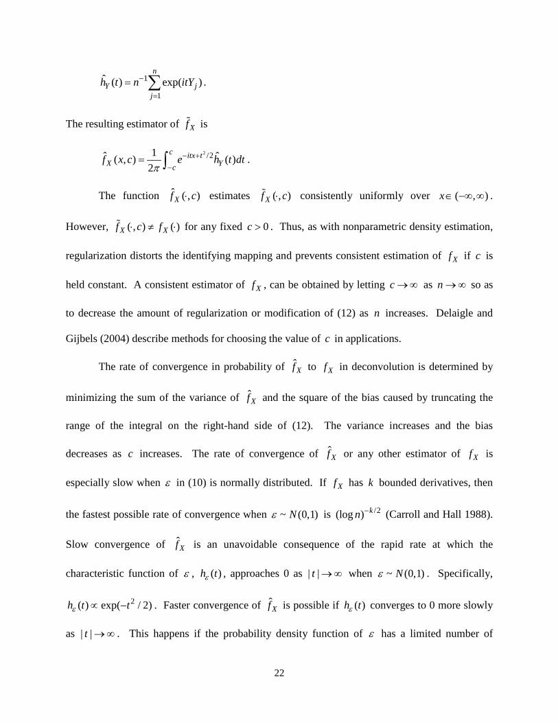
to decrease the amount of regularization or modification of (12) as n increases. Delaigle and

Gijbels (2004) describe methods for choosing the value of c in applications.

The rate of convergence in probability of ˆXf to Xf in deconvolution is determined by

minimizing the sum of the variance of ˆXf and the square of the bias caused by truncating the

range of the integral on the right-hand side of (12). The variance increases and the bias

decreases as c increases. The rate of convergence of ˆXf or any other estimator of Xf is

especially slow when ε in (10) is normally distributed. If Xf has k bounded derivatives, then

the fastest possible rate of convergence when ~ (0,1)Nε is /2(log ) kn − (Carroll and Hall 1988).

Slow convergence of ˆXf is an unavoidable consequence of the rapid rate at which the

characteristic function of ε , ( )h tε , approaches 0 as | |t → ∞ when ~ (0,1)Nε . Specifically,

2( ) exp( / 2)h t tε ∝ − . Faster convergence of ˆXf is possible if ( )h tε converges to 0 more slowly

as | |t → ∞ . This happens if the probability density function of ε has a limited number of

23

derivatives in a neighborhood of the origin (Carroll and Hall 1988, Fan 1991a). For example, if

ε has the Laplace (double exponential) distribution, then ˆXf can converge to Xf at the rate

/(2 5)k kn− + . This rate approaches the parametric rate of 1/2n− if Xf is sufficiently smooth in the

sense of having sufficiently many bounded derivatives. Thus, increased smoothness of the

distribution of X increases the achievable rate of convergence of ˆXf , whereas increased

smoothness of the distribution of ε decreases the achievable rate of convergence of ˆXf . The

practical consequence of slow convergence of ˆXf is that estimating Xf in model (10) accurately

may be impossible if the distribution of ε is very smooth.

The relation between smoothness and the rate of convergence of an estimator carries over

to nonparametric IV estimation of g in model (13). As will be discussed in Section 4.3, the

achievable rate of convergence of an estimator of g becomes faster as g becomes smoother. It

becomes slower as XZf , the probability density function of ( , )X Z , becomes smoother. If XZf

is very smooth – for example if ( , )X Z has a bivariate normal distribution – then the fastest

possible rate of convergence of an estimator of g is (log ) sn − for some 0s > that increases as g

becomes smoother. Thus, as in estimation of Xf in model (10), accurate nonparametric IV

estimation of g may be impossible if the distribution if XZf is very smooth.

4.3 Nonparametric IV Estimation

This section discusses regularization and estimation of the function g in model (13).

There are several methods for regularizing (13). The method discussed here is that of Horowitz

(2011). Similar regularization methods are presented by Blundell, Chen, and Kristensen (2007)

and Newey (2013). Other approaches to regularizing (13) are described by Darolles, Fan,

24

Florens, and Renault (2011); Carrasco, Florens, and Renault (2007); Hall and Horowitz (2005);

and Newey and Powell (2003).

To explain the regularization method and derive the estimator of g , assume that ( , )X Z

in (13) is supported on 2[0,1] . As was explained in Section 2, there is no loss of generality in

this assumption. Let 2[0,1]L denote the set of functions whose squares are integrable on [0,1] .

That is

{ }1 22 0[0,1] : ( )L h h x dx= < ∞∫ .

Define the norm h of any function 2[0,1]h L∈ by

1/21 2

0( )h h x dx = ∫ .

For any functions 1 2 2, [0,1]h h L∈ , define the inner product

1

1 2 1 20, ( ) ( )h h h x h x dx= ∫ .

Finally, define the operator A on 2[0,1]L by

(28) 1

0( )( ) ( , ) ( )XZAh z f x z h x dx= ∫ .

A is the infinite-dimensional generalization of a square matrix. The adjoint of A , denoted by

*A , is defined by the relation

*2 1 2 1, ,A h h h Ah=

for any 1 2 2, [0,1]h h L∈ . *A is the infinite-dimensional generalization of the transpose of a

square matrix. Assume that

25

(29) 1 1 20 0

( , )XZf x z dxdz < ∞∫ ∫ .

Let { : 1,2,...}j jλ = denote the eigenvalues of *A A . That is, jλ satisfies

*jA Ah hλ=

for some function h such that 1h = . Order the eigenvalues so that 1 2 , , , 0λ λ≥ ≥ > . If *A A is

one-to-one and, therefore, invertible, 0jλ > for all j . However, if (29) holds, then 0 is a limit

point of the eigenvalues of *A A . That is, 0jλ → as j → ∞ , and there are infinitely many jλ ’s

within any arbitrarily small neighborhood of 0. This is the source of the ill-posed inverse

problem in nonparametric IV estimation and the consequent need for regularization of (13) to

estimate g .

Now write (15) as

(30) r Ag= .

Equation (30) is a system of infinitely many linear equations in infinitely many unknowns. If A

is one-to-one, then the solution to (30) is

(31) 1g A r−= .

Equivalently,

(32) * 1 *( )g A A A r−= .

Equations (31) and (32) are mappings from the distribution of ( , , )Y X Z to g . Therefore, they

identify g . If A and *A A were finite-dimensional, non-singular matrices, then g could be

estimated consistently by replacing the unknown population quantities A and r with consistent

estimators. However, this procedure does not work when A is infinite dimensional. As is

26

explained by Horowitz (2011), the fact that 0jλ → as j → ∞ guarantees that (31) and (32) are

discontinuous mappings of r to g . Roughly speaking, this is because A and *A A are “nearly

singular” infinite-dimensional matrices. This could not happen if A and *A were finite-

dimensional, because the eigenvalues of a non-singular finite-dimensional matrix are bounded

away from zero.

This problem can be solved and regularization achieved by approximating A by a finite-

dimensional matrix and r by a function that is known up to a finite-dimensional parameter. The

approximations to A and r are constructed so that their approximation errors converge to zero

in an appropriate sense as the dimension of the approximations increases. The resulting

regularized version of g can be estimated consistently by using standard IV methods for linear

models. Of course, the regularized version of g does not satisfy (13). A consistent estimator of

g in (13) can be obtained by letting the dimensions of the finite-dimensional approximations to

A and r increase as the sample size increases. This procedure and the method for implementing

it by using standard IV methods are described in detail in the appendix.

Let J denote the dimension of the finite-dimensional approximations to A and r .

Specifically, the approximation to A is a J J× matrix, and the approximation to r has J

unknown parameters. Denote the resulting estimator of g by ˆJg . A consistent estimator of g

is obtained by letting J → ∞ as n → ∞ . The optimal rate of increase of J is obtained by

minimizing the sum of the (asymptotic) variance of ˆJg and the square of the bias caused by

replacing A and r by finite-dimensional approximations. The variance increases and the bias

decreases as J increases. If g has s derivatives, XZf has q < ∞ derivatives with respect to

any combination of its arguments, and certain other regularity conditions hold, the variance is of

27

order 2 1 /qJ n+ (Horowitz 2012b). Minimizing the sum of the squared bias plus the variance

yields 1/(2 2 1)[ ]s qJ O n + += and

/(2 2 1)ˆ [ ]s s qJ pg g O n− + +− = .

Chen and Reiss (2007) show that /(2 2 1)s s qn− + + is the fastest possible rate of convergence in

probability that is achievable uniformly over functions g and XZf satisfying reasonable

regularity conditions. The rate of convergence of ˆJg to g becomes faster as g becomes

smoother ( s increases) and slower as XZf becomes smoother ( q increases).

The rate of convergence of ˆJg to g is even slower if XZf has infinitely many

derivatives. For example, if XZf is the bivariate normal density (or the density a smooth

monotone transformation of bivariate normals to the unit square), the size of the optimal J is

(log )O n , and the rate of convergence of ˆJg g− is [(log ) ]spO n − . When XZf is very smooth,

the data contain little information about g in (13). Unless g is restricted in other ways, such as

assuming that it belongs to a low-dimensional parametric family of functions, a very large

sample may be needed to estimate g accurately when XZf is very smooth.

The foregoing discussion shows the importance of choosing J well in nonparametric IV

estimation. Indeed, as is explained in Section 4.4, the dependence of J on the sample is the

main difference between parametric and nonparametric estimation of g . The choice of J in

applications is a difficult topic on which research has only recently begun. Newey (2013) and

Horowitz and Lee (2012) describe heuristic methods for choosing J . Horowitz (2012b)

describes a mathematically rigorous way to choose J by minimizing a sample analog of the

asymptotic expectation of 2ˆJg g− .

28

The operator A in (30) must be one-to-one to ensure identification of g in model (13).

This requirement is often called the completeness condition of nonparametric IV estimation and

is the nonparametric analog of the rank condition of parametric IV estimation. If A is not one-

to-one, then (30) is satisfied by two or more different functions g , so g is not identified. The

rank condition of parametric estimation can be tested empirically. In contrast, the condition that

A is one-to-one in nonparametric IV estimation cannot be tested (Canay, Santos, and Shaikh

2013). The condition that A is one-to-one requires the eigenvalues of *A A to exceed zero.

However, as was discussed in the paragraph following (30), there are infinitely many

eigenvalues in any arbitrarily small neighborhood of zero. With a finite sample, regardless of

how large that sample is, random sampling error makes it impossible to distinguish between

eigenvalues that are very close to zero and eigenvalues that are equal to zero. Therefore, with a

finite sample, it is not possible to distinguish empirically between an operator A for which all

the eigenvalues of *A A are strictly positive and an operator for which some eigenvalues of *A A

equal zero.

Now let Jg denote the function that is obtained by replacing A and r in (31) by their

finite-dimensional approximations. The inability to test whether A is one-to-one in applications

and the resulting possibility that g in (13) is not identified does not prevent point estimation of

Jg for a fixed J using the method described in this section. If the J J× matrix approximating

A is non-singular, then ˆJg is a consistent estimator of Jg . Moreover, for each J , the vector

1/2 1/21 1ˆ ˆ[ ( ),..., ( )]J Jn g g n g g ′− − is asymptotically multivariate normally distributed with a mean

of 0. Therefore, inference about Jg can be carried out using the standard methods of parametric

29

IV estimation. Santos (2012) describes some ways to do inference about g when A is not one-

to-one. This is an important topic for future research.

4.4 The Difference between Parametric and Nonparametric IV Estimation

The estimator ˆJg described in Section 4.3 is a standard IV estimator for the parametric

model

1

( ) ; ( | ) 0J

j jj

Y g X U E U Zψ=

= + =∑ ,

where the functions { : 1,2,...}j jψ = are an orthonormal basis for 2[0,1]L . The jg ’s are the

unknown parameters in this model. As is explained in the appendix, they can be estimated

consistently by using standard IV methods for linear models. Therefore, it is reasonable to ask

whether there is any practical difference between parametric and nonparametric IV estimation.

The answer is “yes.” Except in special cases, parametric and nonparametric methods give

different estimates of g , confidence intervals, and outcomes of hypothesis tests. As is discussed

in Horowitz (2011) and Newey (2013), the reason for this is that parametric estimation treats the

model as fixed and exact, whereas nonparametric estimation treats it as an approximation that

depends on the size of the sample. Specifically, in nonparametric estimation, J or the “size” of

the model is larger with large samples than with small ones. In contrast, J is fixed in parametric

estimation. This makes estimates of g based on parametric and nonparametric methods

different unless the value of J used for parametric estimation happens to coincide with the

appropriate value for nonparametric estimation. Moreover, because parametric estimation

assumes a fixed model that does not depend on the sample size, parametric methods typically

30

indicate that the estimates are more precise than they really are. Consequently, conclusions that

are supported by a parametric estimator may not be supported by a nonparametric estimator.

5. INFERENCE

This section discusses methods for forming confidence regions and testing hypotheses in

ill-posed inverse problems. There are important differences between inference in parametric and

nonparametric models, including the nonparametric models that give rise to ill-posed inverse

problems. One difference concerns the relation between optimal point estimators and confidence

regions. In a finite-dimensional parametric model, an asymptotically optimal (or, equivalently,

efficient), asymptotically normal estimator of a parameter can be used to form an asymptotic

confidence interval for the parameter. However, this does not happen in nonparametric

estimation because of the phenomenon of “asymptotic bias.” In nonparametric estimation,

forming confidence intervals and optimal point estimation are separate tasks. A second

difference between parametric and nonparametric models concerns the relation between

confidence regions and hypothesis tests. In a finite-dimensional parametric model, a hypothesis

about the parameter of interest can be accepted or rejected according to whether the hypothesized

value is contained in a confidence region for the parameter. Conversely, a confidence region can

be obtained by inverting a statistic for testing a hypothesis. This duality between confidence

regions and hypothesis tests does not hold in nonparametric models, including models that

present ill-posed inverse problems. A hypothesis test can often be made “more precise” than a

confidence region, and useful confidence regions cannot necessarily be obtained by inverting test

statistics. Consequently, forming confidence regions and testing hypotheses in nonparametric

models are distinct tasks.

31

5.1 Confidence Regions

The estimator of a parameter of a finite-dimensional parametric model usually has a normal

asymptotic distribution that is centered at the true parameter value. Specifically, if θ is an

estimator of a scalar parameter whose true value is 0θ , then

1/20

ˆ( ) / (0,1)dn s Nθθ θ− → ,

where sθ is a standard error. It follows from this result that as n → ∞ ,

1/20

ˆ[ ( ) / ] ( ) ( ) 2 ( ) 1P z n s z z z zθθ θ− < − ≤ → Φ − Φ − = Φ − ,

for any z , where Φ is the standard normal distribution function. Let /2zα denote the 1 / 2α−

quantile of the standard normal distribution. That is, /2zα satisfies

/2( ) 1 / 2zα αΦ = − .

Then an asymptotic 1 / 2α− confidence interval for 0θ is

1/2 1/2/2 0 /2

ˆ ˆn z s n z sα θ α θθ θ θ− −− ≤ ≤ + .

The kernel nonparametric density estimator ˆ ( , )Xf x h in Section 4.1, deconvolution

density estimator ˆ ( , )Xf x c in Section 4.2, and nonparametric IV estimator ˆ ( )Jg x in Section 4.3

are also asymptotically normally distributed for each x . However, the asymptotic distributions

of these estimators are not centered at the true function values, ( )Xf x in the cases of kernel

density estimation and deconvolution density estimation, and ( )g x in the case of nonparametric

IV estimation. Rather, the asymptotic distributions are centered at ( , )Xf x h , ( , )Xf x c , and

( )Jg x for kernel nonparametric density estimation, deconvolution density estimation, and

nonparametric IV estimation, respectively. Thus, as n → ∞

32

(33) 1 1

2 2

3 3

ˆ[ ( , ) ( , )] / ( , )ˆ[ ( , ) ( , )] / ( , ) (0,1)ˆ[ ( ) ( )] / ( , )

n X X nd

n X X n

n J J n

d f x h f x h s x h

d f x c f x c s x c Nd g x g x s x J

−− →−

for any x , where 1nd , 2nd , and 3nd are normalization constants and 1( , )ns x h , 2 ( , )ns x c , and

3( , )ns x J are standard errors. The normalization constants increase without bound as n → ∞ . If

h , c , and J remain fixed as n → ∞ , then 1/21 2 3, ,n n nd d d n= . If h , c , and J change as n

increases so that ˆ ( , )Xf x h , ˆ ( , )Xf h c , and ˆJg , respectively, estimate Xf , Xf , and g

consistently, then 1nd , 2nd , and 3nd increase at rates that depend on the details of the model

being considered but are always slower than 1/2n .

It follows from (33) that as n → ∞

(34) 1 1 1 1ˆ[ ( , ) ( )] / ( , ) [ ( ) / ( , ),1]d

n X X n nd f x h f x s x h N x s x h− → ∆ ,

(35) 2 2 2 2ˆ[ ( , ) ( )] / ( , ) [ ( ) / ( , ),1)d

n X X n nd f x c f x s x c N x s x c− → ∆ ,

and

(36) 3 3 3 3ˆ[ ( ) ( )] / ( , ) [ ( ) / ( , ),1]dn J n nd g x g x s x J N J s x J− → ∆ ,

where

1 1( ) [ ( , ) ( )]n n X Xx d f x h f x∆ = − ,

2 2( ) [ ( , ) ( )]n n X Xx d f x c f x∆ = − ,

and

3 3( ) [ ( ) ( )]n n jx d g x g x∆ = − .

The quantities 1( )n x∆ , 2 ( )n x∆ , and 3( )n x∆ are called asymptotic biases. The word “bias”

applies to the asymptotic distributions of 1ˆ[ ( , ) ( )]n X Xd f x h f x− , 2

ˆ[ ( , ) ( )]n Xd f x c f x− , and

33

3 ˆ[ ( ) ( )]n Jd g x g x− , which are not centered at zero if the corresponding functions nj∆ ( 1,...,3)j =

are non-zero. It follows from (34)-(36) that asymptotic 1 α− confidence intervals for ( )Xf x in

density estimation and deconvolution and ( )g x in nonparametric IV estimation, respectively, are

(37) 1 11 1 /2 1 1 1 /2 1

ˆ ˆ( , ) ( ) ( , ) ( ) ( , ) ( ) ( , )X n n n X X n n nf x h x d z s x h f x f x h x d z s x hα α− −− ∆ − ≤ ≤ − ∆ − ,

(38) 1 12 2 /2 2 2 2 /2 2

ˆ ˆ( , ) ( ) ( , ) ( ) ( , ) ( ) ( , )X n n n X X n n nf x c x d z s x c f x f x c x d z s x cα α− −− ∆ − ≤ ≤ − ∆ − ,

and

(39) 1 13 3 /2 3 3 3 /2 3ˆ ˆ( ) ( ) ( , ) ( ) ( ) ( ) ( , )J n n n J n n ng x x d z s x J g x g x x d z s x Jα α

− −− ∆ − ≤ ≤ − ∆ − .

The asymptotic bias terms, ( )nj x∆ ( 1,...,3)j = depend on population parameters that are

unknown in applications, and the standard errors nks ( 1,...,3k = ) converge to non-zero limits as

n → ∞ . Therefore, the confidence intervals (37)-(39) cannot be used in applications unless the

bias terms converge to zero as n → ∞ more rapidly than the inverses of the normalization

factors, 1njd − ( 1,...,3j = ). Equivalently, feasibility of (37)-(39) in applications requires

2 2( ) ( )nj njx o d −∆ = as n → ∞ . However, the optimal values of the regularization parameters, h ,

c , and J , minimize the mean-square errors (MSE’s) of the corresponding estimators or,

possibly, integrals of the MSE’s over the range of x . The MSE’s are the squares of the biases

plus the variances of the estimators. Thus, for example, the MSE of the kernel nonparametric

density estimator ˆ ( , )Xf x h is

2 2 2 21 1 1

ˆ[ ( , ) ( )] ( ) ( , )X X n n nE f x h f x x d s x h−− ≈ ∆ +

when n is large. Similar expressions hold for deconvolution and nonparametric IV estimators.

34

Because the asymptotic variance term 2njs ( 1,...,3j = ) converges to a non-zero limit as

n → ∞ , the optimal value of the regularization parameter equates the rates of convergence of

2( )nj x∆ and 2njd − . Therefore, the asymptotic bias is non-negligible. Moreover, it can be shown

that the optimal regularization parameter also achieves the fastest possible rates of convergence

in probability of ˆ ( , )Xf x h , ˆ ( , )Xf x c , and ˆ ( )Jg x to ( )Xf x , ( )Xf x , and ( )g x , respectively.

Because the choices of regularization parameters that produce asymptotically optimal point

estimators of ( )Xf x and ( )g x have non-negligible asymptotic biases, these estimators cannot be

used to form confidence intervals in applications. In contrast to the situation with finite-

dimensional parametric models, nonparametric point estimation of ( )Xf x and ( )g x and

formation of confidence intervals for these quantities are distinct tasks. Methods for dealing

with asymptotic bias are described in the paragraphs below. All methods produce confidence

intervals that are wider than the intervals that would be obtained from (37)-(39) if the nj∆ ’s were

known and asymptotically optimal values of the regularization parameters were used. Relatively

wide confidence intervals are unavoidable in nonparametric estimation.

The asymptotic bias terms in (37)-(39) are caused by regularization. They decrease as

the amount of regularization decreases (that is, as h decreases and c or J increase). In

addition, njd ’s decrease as the amount of regularization decreases. Therefore, the asymptotic

bias terms can be made negligible by using less than the optimal amount of regularization (that

is, choosing a value of h that decreases more rapidly than the optimal rate for kernel

nonparametric density estimation and values of c and J that increase more rapidly than the

optimal rates for deconvolution density estimation and nonparametric IV estimation). This is

called “undersmoothing.” The main problem with undersmoothing is that although empirical

35

methods are available for estimating the optimal value of the regularization parameter in many

applications, there is no satisfactory empirical way to choose an undersmoothed value. At

present, the undersmoothed parameter value must be chosen by using an essentially arbitrary rule

of thumb. For example, one might use the estimated optimal parameter value to a power that is

less than one in the case of kernel density estimation and greater than one in the case of

deconvolution density estimation or nonparametric IV estimation.

Having selected an undersmoothed value of the regularization parameter by using a rule

of thumb or other method, a confidence interval can be constructed by dropping the asymptotic

bias terms from (37)-(39). Methods for calculating the required standard errors are presented by

(Silverman 1978), among others, for kernel nonparametric density estimation; Fan (1991b) for

deconvolution density estimation; and Horowitz (2007), Horowitz and Lee (2012), and Newey

(2013) for nonparametric IV estimation.

Another way to deal with asymptotic bias is to estimate ( )nj x∆ and subtract the

estimated bias from the estimator of ( )Xf x or ( )g x . In the case of kernel nonparametric density

estimation, for example, this procedure replaces ˆ ( )Xf x with 1ˆ ˆ( ) ( )X nf x x− ∆ , where 1

ˆ ( )n x∆ is

the estimator of 1( )n x∆ . This procedure is called explicit bias correction. Schucany and

Sommers (1977) describe a simple procedure for carrying out explicit bias correction in kernel

nonparametric density estimation. Similar procedures can be developed for deconvolution

density estimation and nonparametric IV estimation, although this has not been done. Explicit

bias correction requires selection of an auxiliary value of the regularization parameter for use in

estimating the bias. Satisfactory empirical methods for doing this have not been developed.

A third way to deal with asymptotic bias is to modify the critical value, /2zα , so that a

confidence interval that is based on a conventional estimate of the asymptotically optimal

36

regularization parameter but ignores asymptotic bias has the correct asymptotic coverage

probability. In the case of kernel nonparametric density estimation, the resulting

1 α− confidence interval is

1 11 1 1 1

ˆ ˆ( , ) ( ) ( ) ( , ) ( )X n n X X n nf x h zd s x f x f x h zd s x− −− ≤ ≤ + ,

where z is the modified critical value. Hall and Horowitz (2013) present a bootstrap-based

method for selecting z for nonparametric density estimation. This method has the advantage of

not requiring selection of a value of h that undersmooths or an auxiliary value for bias

estimation. It is likely that the method can be extended to deconvolution and nonparametric IV

estimators, but the required research has not yet been carried out.

Regardless of how asymptotic bias is handled, confidence intervals based on (37)-(39)

are pointwise intervals. That is, they have the correct asymptotic coverage probabilities at only

one value of x . They do not have correct coverage probabilities simultaneously at several or a

continuum of values of x . A band that contains ( )Xf x or ( )g x with known probability for all

values of x is called a uniform confidence band. A uniform confidence band is wider than a

pointwise confidence band with the same coverage probability. The general form of a uniform

confidence band is

(40) |Estimated function( ) True function( ) | ( ) for all x x z x x− ≤ ,

where ( )z x depends on the details of the estimation problem and is chosen so that (40) holds

asymptotically with a specified probability.

Bickel and Rosenblatt (1973) derive a uniform confidence band for Xf based on kernel

nonparametric density estimation. Bissantz, Dümbgen, Holtzmann, and Munk (2007) derive a

uniform band for ( )Xf x based on a deconvolution density estimator and present a bootstrap

method for implementing the band. The bands for nonparametric density estimation and

37

deconvolution are obtained by showing that suitably centered and normalized differences

between the estimated and true functions converge to a Gaussian process as n → ∞ . Horowitz

and Lee (2012) present a bootstrap method for obtaining a uniform confidence band for g in

nonparametric IV estimation. They use the bootstrap to obtain joint confidence intervals for a

normalized version of 1 1ˆ ˆ( ) ( ),..., ( ) ( )J J K Kg x g x g x g x− − on a discrete set of points 1,..., Kx x .

They then show that a uniform confidence band for g can is obtained by letting the number of

points, K , increase to ∞ and the distance between points decrease to 0 as n → ∞ .

4.2 Hypothesis Tests

This section discusses tests of hypotheses about a function whose estimation presents an

ill-posed inverse problem. The discussion focusses on nonparametric IV estimation and shows

that it is possible to construct powerful tests of hypotheses about the function g in (13), despite

the imprecision of estimates of g that is an unavoidable consequence of the ill-posed inverse

problem. As is discussed briefly at the end of this section, methods similar to those described

here for nonparametric IV estimation are available for kernel nonparametric density estimation

and deconvolution density estimation.

A hypothesis about g in (13) (the null hypothesis) can be written

0 :H g ∈ ,

where is a set of functions in 2[0,1]L . For example, the hypothesis that g belongs to a

specified, finite-dimensional parametric family corresponds to

(41) { ( , ) : }G x θ θ= ∈Θ ,

38

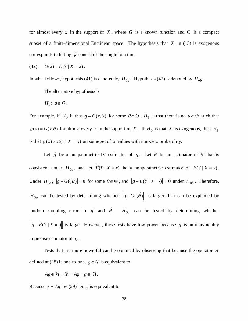
for almost every x in the support of X , where G is a known function and Θ is a compact

subset of a finite-dimensional Euclidean space. The hypothesis that X in (13) is exogenous

corresponds to letting consist of the single function

(42) ( ) ( | )G x E Y X x= = .

In what follows, hypothesis (41) is denoted by 0aH . Hypothesis (42) is denoted by 0bH .

The alternative hypothesis is

1 :H g ∉ .

For example, if 0H is that ( , )g G x θ= for some θ ∈Θ , 1H is that there is no θ ∈Θ such that

( ) ( , )g x G x θ= for almost every x in the support of X . If 0H is that X is exogenous, then 1H

is that ( ) ( | )g x E Y X x≠ = on some set of x values with non-zero probability.

Let g be a nonparametric IV estimator of g . Let θ be an estimator of θ that is

consistent under 0aH , and let ˆ ( | )E Y X x= be a nonparametric estimator of ( | )E Y X x= .

Under 0aH , ( , ) 0g G θ− ⋅ = for some θ ∈Θ , and ( | ) 0g E Y X− = ⋅ = under 0bH . Therefore,

0aH can be tested by determining whether ˆˆ ( , )g G θ− ⋅ is larger than can be explained by

random sampling error in g and θ . 0bH can be tested by determining whether

ˆˆ ( | )g E Y X− = ⋅ is large. However, these tests have low power because g is an unavoidably

imprecise estimator of g .

Tests that are more powerful can be obtained by observing that because the operator A

defined at (28) is one-to-one, g ∈ is equivalent to

{ : }Ag h Ag g∈ = = ∈ .

Because r Ag= by (29), 0aH is equivalent to

39

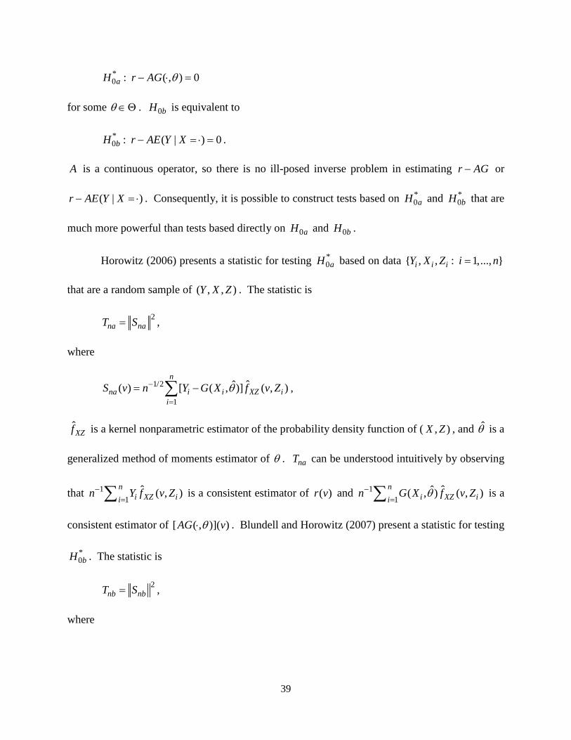
*0 : ( , ) 0aH r AG θ− ⋅ =

for some θ ∈Θ . 0bH is equivalent to

*0 : ( | ) 0bH r AE Y X− = ⋅ = .

A is a continuous operator, so there is no ill-posed inverse problem in estimating r AG− or

( | )r AE Y X− = ⋅ . Consequently, it is possible to construct tests based on *0aH and *

0bH that are

much more powerful than tests based directly on 0aH and 0bH .

Horowitz (2006) presents a statistic for testing *0aH based on data { , , : 1,..., }i i iY X Z i n=

that are a random sample of ( , , )Y X Z . The statistic is

2na naT S= ,

where

1/2

1

ˆˆ( ) [ ( , )] ( , )n

na i i XZ ii

S v n Y G X f v Zθ−

=

= −∑ ,

ˆXZf is a kernel nonparametric estimator of the probability density function of ( , )X Z , and θ is a

generalized method of moments estimator of θ . naT can be understood intuitively by observing

that 11

ˆ ( , )ni XZ ii

n Y f v Z−=∑ is a consistent estimator of ( )r v and 1

1ˆˆ( , ) ( , )n

i XZ iin G X f v Zθ−

=∑ is a

consistent estimator of [ ( , )]( )AG vθ⋅ . Blundell and Horowitz (2007) present a statistic for testing

*0bH . The statistic is

2nb nbT S= ,

where

40

1/2

1

ˆˆ( ) [ ( )] ( , )n

nb i i XZ ii

S v n Y G X f v Z−

=

= −∑ ,

ˆXZf is again a kernel nonparametric estimator of the probability density function of ( , )X Z , and

ˆ ( )G ⋅ is kernel nonparametric regression estimator of ( | )E Y X = ⋅ . nbT can be understood

intuitively by observing that 11

ˆˆ ( ) ( , )ni XZ ii

n G X f v Z−=∑ is a consistent estimator of

[ ( | )]( )AE Y X v= ⋅ .

Under *0aH and *

0bH (or, equivalently, 0aH and 0bH ), the statistics naT and nbT are

asymptotically distributed as weighted sums of independent random variables that have chi-

squared distributions with one degree of freedom. Horowitz (2006) and Blundell and Horowitz

(2007) present methods for computing critical values for naT and nbT . In addition, Horowitz

(2006) and Blundell and Horowitz (2007) show that tests based on naT and nbT have non-trivial

power against alternative hypotheses whose distances from *0aH and *

0bH (or, equivalently, 0aH

and 0bH ) are 1/2( )O n− . Non-trivial power means that the probability of rejecting a false null

hypothesis exceeds the level of the test. naT and nbT have non-trivial power against alternatives

that are much closer to the null hypotheses of these statistics than is possible with tests based on

ˆˆ ( , )g G θ− ⋅ and ˆˆ ( | )g E Y X− = ⋅ .

Because of the unavoidable imprecision of estimates of g in model (13), the half-width

of a confidence interval for g is always larger than 1/2( )O n− and can be as large as [(log ) ]sO n −

for some finite 0s > . In contrast, tests based on naT and nbT have non-trivial power against

alternative hypotheses whose distance from the null hypothesis is 1/2( )O n− and power

41

approaching 1 as n → ∞ against alternatives whose distance from the null hypothesis exceeds

1/2( )O n− . Therefore, these tests can detect an erroneous null hypothesis about g whose distance

from the correct alternative hypothesis is much smaller than the half-width of a confidence

interval for g . This is the sense in which a hypothesis test can be more precise than a

confidence region.

Methods similar those just discussed are applicable to testing hypotheses about Xf in

kernel nonparametric density estimation and deconvolution density estimation. Both estimation

problems begin with an operator equation of the form

Xh Bf= ,

where h is an easily estimated function and B is a continuous, one-to-one operator that is

known in the cases of kernel density estimation and deconvolution density estimation.

Accordingly, testing the hypothesis Xf ∈ for a suitable set is equivalent to testing the

hypothesis that 0Xh Bf− = for some Xf ∈ . Statistics similar to naT and nbT can be used to

test this hypothesis.

6. AN EMPRICAL ILLUSTRATION

This section presents an empirical example consisting of nonparametric IV estimation of

an Engel curve for food. The data are 1655 household-level observations from the British

Family Expenditure Survey. The households consist of married couples with an employed head-

of-household between the ages of 25 and 55 years. The model is specified as in (13). In this

model, Y denotes a household's expenditure share on food, X denotes the logarithm of the

household’s total expenditures, and Z denotes the logarithm of the household’s gross earnings.

The basis functions are B-splines with four knots. The estimation method is that of Section 4.3.

42

The Engel curve estimated here is the same as the one reported by Horowitz (2011). The

results presented in this section include a uniform 95 percent confidence band as well as the

estimated Engel curve. Blundell, Chen, and Kristensen (2007) used data from the Family

Expenditure Survey in nonparametric IV estimation of Engel curves and investigated the validity

of Z as an instrument for X .

The estimated Engel curve and a uniform 95 percent confidence band for the unknown

true Engel curve are shown in Figure 1. The uniform confidence band is obtained using the

methods of Horowitz and Lee (2012). It can be seen from Figure 1 that the estimated curve is

nonlinear and different from what would be obtained with a linear, quadratic, or cubic model.

The hypotheses that the Engel curve is quadratic or cubic is rejected by Horowitz’s (2006) test of

hypothesis 0aH ( 0.05p < in both cases). Thus, the nonparametric estimate provides

information about the shape of the Engel curve that would be difficult to obtain using

conventional parametric methods.

The average half-width of the confidence band is approximately 40 percent of the

estimated value of g . The band is wide because of the unavoidable imprecision of

nonparametric IV estimates. These estimates are imprecise because the data contain little

information about g in model (13). Of course, a sufficiently careful specification search may

produce a parametric model that gives a curve similar to the nonparametric one and the

appearance of greater precision. However, a specification search provides no information about

the accuracy of the curve it produces, and its results cannot be used for statistical inference. A

confidence band based on a model found through a specification search would be misleadingly

narrow. Its apparent or nominal coverage probability would be much larger than its true

coverage probability.

43

7. CONCLUSIONS

The term “ill-posed inverse problem” refers to a condition in which the mapping from the

population distribution of observables to the object identified by a statistical or econometric

model is discontinuous. Moreover, in an ill-posed inverse problem, the identified object cannot

be estimated consistently by replacing the population distribution with a consistent sample

analog. This paper has presented examples of ill-posed inverse problems in economics and other

fields. The paper has explained how ill-posedness arises, why it causes difficulty for estimation

and inference, and how estimation and inference can be carried out.

Ill-posed inverse problems have been studied in mathematics and related fields for over

100 years and have recently been the objects of intensive research in econometrics. Methods for

estimation and inference in ill-posed inverse problems are used routinely in many fields, but

there have been few economic applications of these methods. This is undoubtedly due in part to

the newness of methods such as nonparametric IV estimation. Another possible reason is that

models that give rise to ill-posed inverse problems are semi- or nonparametric, whereas

economists tend to prefer finite-dimensional parametric models for empirical research.

However, economic theory does not provide parametric models. A parametric model is arbitrary

and can be highly misleading. This is true even if it is obtained through a specification search in

which several different models are estimated and conclusions are based on the one that appears

to fit the data best. There is no guarantee that a specification search will include the correct

model or a good approximation to it, and there is no guarantee that the correct model will be

selected if it happens to be included in the search. Moreover, a model obtained through a

specification search cannot be used for valid statistical inference.

44

Applications of nonparametric methods, including methods for ill-posed inverse

problems, that have been carried out so far demonstrate the feasibility of these methods in

empirical economics and the ability of the methods to provide results that differ in important

ways from those obtained with standard parametric models. See, for example, Blundell, Chen,

and Kristensen (2007); Blundell, Horowitz, and Parey (2012); Haag, Hoderlein, and Pendakur

(2009); Hausman and Newey (1995); Hoderlein and Holzmann (2011); Horowitz (2011); and

Horowitz and Härdle (1996). Even an imprecise semi- or nonparametric estimate can be useful

by revealing the extent to which conclusions drawn from a parametric model are consequences

of the parametric assumptions as opposed to information contained in the data (Horowitz 2011).

Thus, semi- and nonparametric methods, including methods for estimation and inference in ill-

posed inverse problems, have much to offer empirical economics.

8. APPENDIX

8.1 An Example that Illustrates the Discontinuity of the Inverse of Mapping (15)

Let

1/2

1( , ) ( ) ( ); 0 , 1XZ j j j

jf x z x z x zλ φ φ

∞

=

= ≤ ≤∑ ,

where 1( ) 1vφ = , ( ) 2 cos[( 1) ]j v j vφ π= − for 2j ≥ , 1 1λ = , and 40.2( 1)j jλ −= − for 2j ≥ .

With this XZf , the marginal distributions of X and Z are uniform on [0,1] , but X and Z are

not independent of one another. Moreover, the functions jφ are orthonormal. That is,

1

1

1 if ( ) ( )

0 if j kj k

v v dvj k

φ φ−

== ≠∫

Under very general conditions ( )r z has the infinite series representation

45

1

( ) ( )j jj

r z c zφ∞

=

= ∑ ,

where the coefficients { }jc satisfy 21 jjc∞

=< ∞∑ . It follows from Picard’s theorem for integral

equations (Kress 1999, Theorem 15.18) that

(43) 1/21

( ) ( )jj

jj

cg x xφ

λ

∞

=

= ∑ .

Now, let 0δ > be an arbitrary constant, and define

3/2

2( ) ( ) ( 1) ( )j j

jr z r z j zδ φ

∞−

=

= + −∑ .

Then 0 1sup | ( ) ( ) |z r z r z≤ ≤ − can be made arbitrarily small by letting δ be sufficiently small.

However, it follows from (43) that with r in place of r , the solution to (15) is

1/2 3/22

1( ) ( ) ( )( 1) j

jjg x g x x

jδ φ

λ

∞

=

= +−∑

and that

1 21[ ( ) ( )]g x g x dx

−− = ∞∫ .

Thus, the difference between ( )g x and ( )g x is infinite on a set of x values with positive

Lebesgue measure, although the difference between ( )r x and ( )r x may be arbitrarily small.

8.2 Procedure for Regularizing and Estimating g in Model (13)

The procedure has two steps: (1) Form finite-dimensional approximations to r and A ,

and form the regularized version of (31); (2) consistently estimate unknown population quantities

in the approximations to obtain the regularized estimator of g .

46

Step 1: To form the desired approximations to r and A , let { : 1, 2,...}j jψ = be an

orthonormal basis for 2[0,1]L . Then we can write

(44) 1

( ) ( )j jj

r z r zψ∞

=

= ∑

and

(45) 1 1

( , ) ( ) ( )XZ jk j kj k

f x z a x zψ ψ∞ ∞

= =

= ∑∑ ,

where ,j jr r ψ= and

1 1

0 0( ) ( ) ( , )jk j k XZa x z f x z dxdzψ ψ= ∫ ∫ .

Moreover, for any 2[0,1]h L∈ ,

1 1

( )( ) , ( )jk j kj k

Ah z a h zψ ψ∞ ∞

= =

= ∑∑ .

In particular,

1 1

( )( ) , ( )jk j kj k

Ag z a g zψ ψ∞ ∞

= =

= ∑∑ .

The finite-dimensional approximations to r and A are obtained by truncating the series

(44) and (45) at J < ∞ terms. Let Jr and JA denote the resulting approximations. Then

1

( ) ( )J

J j jj

r z r zψ=

= ∑ ,

and for any 2[0,1]h L∈ ,

1 1

( )( ) , ( )J J

J jk j kj k

A h z a h zψ ψ= =

= ∑∑ .

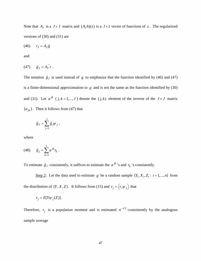
47

Note that JA is a J J× matrix and ( )( )JA h z is a 1J × vector of functions of z . The regularized

versions of (30) and (31) are

(46) J Jr A g=

and

(47) 1

J Jg A r−

= .

The notation Jg is used instead of g to emphasize that the function identified by (46) and (47)

is a finite-dimensional approximation to g and is not the same as the function identified by (30)

and (31). Let jka ( , 1,...,j k J= ) denote the ( , )j k element of the inverse of the J J× matrix

[ ]jka . Then it follows from (47) that

1

J

J j jj

g g ψ=

= ∑ ,

where

(48) 1

Jjk

j kk

g a r=

= ∑ .

To estimate Jg consistently, it suffices to estimate the jka ’s and kr ’s consistently.

Step 2: Let the data used to estimate g be a random sample { , , : 1,..., }i i iY X Z i n= from

the distribution of ( , , )Y X Z . It follows from (15) and ,j jr r ψ= that

[ ( )]j jr E Y Zψ= .

Therefore, jr is a population moment and is estimated 1/2n− -consistently by the analogous

sample average

48

1

1

ˆ ( )n

j i j ii

r n Y Zψ−

=

= ∑ .

In addition, jka is the population moment

[ ( ) ( )]jk j ka E X Zψ ψ=

and is estimated 1/2n− consistently by the sample average

1

1

ˆ ( ) ( )n

jk j i k ii

a n X Zψ ψ−

=

= ∑ .

JA is estimated consistently by the operator ˆJA , which is defined by

1 1

ˆ ˆ( )( ) , ( )J J

J jk j kj k

A h z a h zψ ψ= =

= ∑∑

for any function 2[0,1]h L∈ . Let ˆ jka ( , 1,...,j k J= ) denote the ( , )j k element of the inverse of

the J J× matrix ˆ[ ]jka . Then the sample analog of (48) is

1

ˆ ˆ ˆJ

jkj k

kg a r

=

= ∑ .

Moreover, for any J < ∞ , Jg is estimated consistently by

(49) 1

ˆ ˆJ

J j jj

g g ψ=

= ∑ .

In particular, as n → ∞ ˆ 0pJ Jg g− → , and ˆ 0p

Jg g− → if J → ∞ at a suitable rate.

The estimator ˆJg in (49) can be put into the form of a conventional linear IV estimator,

which makes it easy to compute ˆJg using standard software. Let and , respectively,

49

denote the n J× matrices whose ( , )i j elements are ( )j iZψ and ( )j iXψ . Define the 1n×

vector 1( ,..., )nY Y ′= . Define the 1J × vector 1ˆ ˆ ˆ( ,..., )JG g g ′= . Then (49) is equivalent to

1ˆ ( )G −′ ′= .

G has the form of an IV estimator for a linear model in which the matrix of variables is and

the matrix of instruments is .

50

REFERENCES

Bickel, P.J., Rosenblatt, M. 1973. On some global measures of the deviations of density function

estimates. Annals of Statistics. 1:1071-1095.

Bissantz, N., Dümbgen, L., Holtzmann, H., Munk, A. 2007. Non-parametric confidence bands

in deconvolution density estimation. Journal of the Royal Statistical Society, Series B.

69:483-506.

Blundell, R., Chen, X., Kristensen, D. 2007. Semi-nonparametric IV estimation of shape-

invariant Engel curves. Econometrica. 75:1613-1669.

Blundell, R., Horowitz, J.L. 2007. A non-parametric test of exogeneity. Review of Economic

Studies. 74:1035-1058.

Blundell, R., Horowitz, J.L., and Parey, P. 2012. Measuring the price responsiveness of

gasoline demand: economic shape restrictions and nonparametric demand estimation.

Quantitative Economics. 3:29-51.

Blundell, R., Powell, J.L. 2003. Endogeneity in nonparametric and semiparametric regression

models. In Advances in Economics and Econometrics: Theory and Applications, Eighth

World Congress Vol. II, ed. M. Dewatripont, L.P. Hansen, and S.J. Turnovsky, pp. 312-357.

Cambridge, U.K.: Cambridge University Press. 77:491-533.

Bonhomme, S. and Robin, J.-M. 2010. Generalized non-parametric deconvolution with an

application to earnings dynamics. Review of Economic Studies. 77:491-533.

Canay, I.A., Santos, A., and Shaikh, A.M. 2013. On the testability of identification in some

nonparametric models with endogeneity. Econometrica. Forthcoming.

Carrasco, M. Florens, J.-P., Renault, E. 2007.Linear inverse problems in structural econometrics

estimation based on spectral decomposition and regularization. In Handbook of Econometrics

51

Vol. 6B, ed. J.J. Heckman and E.E. Leamer, pp. 5633-5751. Amsterdam: Elsevier Science

B.V.

Carroll, R.J., Hall, P. 1988. Optimal rates of convergence for deconvolving a density. Journal

of the American Statistical Association. 83:1184-1186.

Chalmond, B. 2003. Modeling and Inverse Problems in Image Analysis. New York: Springer-

Verlag.

Chen, X. 2007. Large sample sieve estimation of semi-nonparametric models. In Handbood of

Econometrics Vol. 6B, ed. J.J. Heckman and E.E. Leamer, pp. 5592-5632. Amsterdam:

Elsevier Science B.V.

Chen, X., Hong, H., Nekipilov, D. 2011. Nonlinear models of measurement errors. Journal of

Economic Literature. 49:901-937.

Chen, X., Pouzo, D. 2012. Estimation of nonparametric conditional moment models with

possibly nonsmooth generalized residuals. Econometrica. 80:277-321.

Chen, X. and Reiss, M. 2007. On rate optimality for ill-posed inverse problems in econometrics.

Econometric Theory. 27:497-521.

Darolles, S., Fan, Y., Florens, J.-P., Renault, E. 2011. Nonparametric instrumental regression.

Econometrica. 79:1541-1565.

Delaigle, A., Gijbels, I. 2004. Practical bandwidth selection in deconvolution kernel density

estimation. Computational Statistics and Data Analysis. 45:249-267.

Delaigle, A., Hall, P., Meister, A. 2008. On deconvolution with repeated measurements.

Annals of Statistics. 36:665-685.

Engl, H.W., Hanke, M., Neubauer, A. 1996. Regularization of Inverse Problems. Dordrecht:

Kluwer Academic Publishers.

52

Fan, J. 1991a. On the optimal rates of convergence for nonparametric deconvolution problems.

Annals of Statistics. 19:1257-1272.

Fan, J. 1991b. Asymptotic normality for deconvolution kernel density estimators. Sankhya

Series A. 53:97-110.

Gautier, E. and Kitamura, Y. 2013. Nonparametric estimation in random coefficents binary

choice models. Econometrica. 81:581-606.

Haag, B.R., Hoderlein, S., and Pendakur, K. 2009. Testing and imposing Slutsky symmetry in

nonparametric demand systems. Journal of Econometrics. 153:33-50.

Hadamard, J. 1923. Lectures on Cauchy’s Problem in Linear Partial Differential Equations.

New Haven: Yale University Press.

Härdle, W., Linton, O. 1994. Applied nonparametric methods. In Handbook of Econometrics,

Vol. IV, ed. R.F. Engle and D. McFadden, pp. 2295-2339. Amsterdam: Elsevier Science B.V.

Hall, P., Horowitz J.L. 2005. Nonparametric methods for inference in the presence of

instrumental variables. Annals of Statistics. 33:-2904-2929.

Hall, P., Horowitz, J.L. 2013. A simple bootstrap method for constructing nonparametric

confidence bands for functions. Annals of Statistics. Forthcoming.

Hausman, J.A. and Newey, W.K. 1995. Nonparametric estimation of exact consumer surplus

and deadweight loss. Econometrica. 63:1445-1476.

Hoderlein, S. and Holzmann, H. 2011. Demand analysis as an ill posed inverse problem with

semiparametric specification. Econometric Theory. 27:609-638.

Hoderlein, S., Klemelä, J., and Mammen, E. 2010. Analyzing the random coefficient model

nonparametrically. Econometric Theory. 26:804-837.

53

Horowitz, J.L. 2006. Testing a parametric model against a nonparametric alternative with

identification through instrumental variables. Econometrica. 74:521-538.

Horowitz, J.L. 2007. Asymptotic normality of a nonparametric instrumental variables estimator.

International Economic Review. 48:1349.

Horowitz, J.L. 2011. Applied nonparametric instrumental variables estimation. Econometrica.

79:347-394.

Horowitz, J.L. 2012a. Specification testing in nonparametric instrumental variables estimation.

Journal of Econometrics. 167: 383-396.

Horowitz, J.L. 2012b. Adaptive nonparametric instrumental variables estimation: empirical

choice of the regularization parameter. Working paper, Department of Economics, Northwestern

University.

Horowitz, J.L. and Härdle, W. 1996. Direct semiparametric estimation of single-index models

with discrete covariates. Journal of the American Statistical Association. 91: 1632-1640.

Horowitz, J.L., Lee, S. 2007. Nonparametric instrumental variables estimation of a quantile

regression model. Econometrica. 75:1191-1208.

Horowitz, J.L. and Lee, S. 2012. Uniform confidence bands for functions estimated

nonparametrically with instrumental variables. Journal of Econometrics. 168:175-188.

Horowitz, J.L., Markatou, M. 1996. Semiparametric estimation of regression models for panel

data. Review of Economic Studies. 63:145-168.

Huber, P.J. 1981. Robust Statistics. New York: John Wiley & Sons.

Johannes, J. 2009. Deconvolution with unknown error distribution. Annals of Statistics.

37:2301-2323.

Kress, R. 1999. Linear Integral Equations, 2nd edition. New York: Springer-Verlag.

54

Li, T. 2002. Robust and consistent estimation of nonlinear errors-in-variables models. Journal

of Econometrics. 110:1-26.

Li, T., Hsiao, C. 2004. Robust estimation of generalized linear models with measurement errors.

Journal of Econometrics. 118:51-65.

Li, T., Perrigne, I., Vuong, Q. 2000. Conditionally independent private information in OCS

wildcat auctions. Journal of Econometrics. 98:129-161.

Linton, O., Whang, Y,-J. 2002. Nonparametric estimation with aggregated data. Econometric

Theory. 18:420-468.

Manski, C.F. 1988. Analog Estimation Methods in Econometrics. London: Chapman & Hall.

Natterer, F. 1986. The Mathematics of Computerized Tomography. New York: John Wiley &

Sons.

Natterer, F., Wubbeling, F. 2001. Mathematical Methods in Image Reconstruction.

Philadelphia: Society for Industrial and Applied Mathematics.

Newey, W.K. 2013. Nonparametric instrumental variables estimation. American Economic

Review: Papers and Proceedings. 103:550-556.

Newey, W.K., Powell, J.L. 2003. Instrumental variable estimation of nonparametric models.

Econometrica. 71:1565-1578.

Newey, W.K., Powell, J.L., Vella, F. 1999. Nonparametric estimation of triangular

simultaneous equations models. Econometrica. 67: 565-603.

O’Sullivan, F. 1986. A statistical perspective on ill-posed inverse problems. Statistical Science.

1:502-518.

55

Radon, J. 1917. Über die Bestimmung von Funktionen durch ihre Integralwerte längs gewisser

Mannigfaltigkeiten. Berichte Über die Verhadlungen der Königlich-Sächsischen Akademie

der Wissenshaften zu Leipzig, Mathematisch-Physische Klasse. 69: 262-277.

Rao, C.R. 1973. Linear Statistical Inference and Its Applications, 2nd edition. New York: John

Wiley & Sons.

Santos, A. 2012. Inference in nonparametric instrumental variables with partial identification.

Econometrica. 80:213-275.

Schennach, S.M. 2004a. Estimation of nonlinear models with measurement error.

Econometrica. 72:33-75.

Schennach, S.M. 2004b. Nonparametric regression in the presence of measurement error.

Econometric Theory. 20:1046-1093.

Schucany, W.R., Sommers, J.P. 1977. Improvement of kernel type density estimators. Journal

of the American Statistical Association. 72:420-423.

Silverman, B. W. 1978. Weak and strong uniform consistency of the kernel estimate of a density

and its derivatives. Annals of Statistics. 6: 177-184.

Silverman, B. W. 1986. Density Estimation for Statistics and Data Analysis. London: Chapman

& Hall.

Stone, C.J. 1982. Optimal global rates of convergence for nonparametric regression. Annals of

Statistics. 10:1040-1053.

56

0.1

.2.3

Exp

endi

ture

Sha

re

4 5 6 7 8Log of Total Expenditures

Figure 1

Nonparametric IV Estimate of an Engel curve. Solid line is the estimated curve. Dashed lines

indicate a uniform 95 percent confidence band for the unknown true curve.