Ijsom19021398886200

38

International Journal of Supply and Operations Management

IJSOM

May 2014, Volume 1, Issue 1, pp. 38-53

ISSN: 2383-1359

ccc.mosww.www

Location-routing problem with fuzzy time windows and traffic time

Shima Teimooria, Hasan Khademi Zare

b and Mohammad Saber Fallah Nezhad

b

a Department of Industrial Engineering, Elmo Honar University

b Department of Industrial Engineering, Yazd University

Abstract

The location-routing problem is a relatively new branch of logistics system. Its objective is to

determine a suitable location for constructing distribution warehouses and proper transportation

routing from warehouse to the customer. In this study, the location-routing problem is investigated

with considering fuzzy servicing time window for each customer. Another important issue in this

regard is the existence of congested times during the service time and distributing goods to the

customer. This caused a delay in providing service for customer and imposed additional costs to

distribution system. Thus we have provided a mathematical model for designing optimal distributing

system. Since the vehicle location-routing problem is Np-hard, thus a solution method using genetic

meta-heuristic algorithm was developed and the optimal sequence of servicing for the vehicle and

optimal location for the warehouses were determined through an example.

Keywords: Locating Routing; fuzzy time window; satisfaction level; congested times

1. Introduction

Today, rising energy costs and increasing competition have forced logistics sector to improve the

efficiency of transportation network. Network design is a fundamental step in designing an effective

supply chain. There are many different decisions in distribution network design that consists of

determining the optimal location of facilities of supply chain. These decisions are generally

categorized in strategic, tactical and operational levels. Strategic or long-term decisions require high

investment and have vital importance for firms in order to survive among competitors. Tactical

Corresponding author email address: [email protected]

http://www.ijsom.com/

Int J Supply Oper Manage (IJSOM)

39

decisions consist of midterm decisions. Operational decisions mostly include tasks scheduling that

are performed regularly (Fazel-Zarandi et al., 2013). Location routing problem as a relatively new

branch of logistics system, includes strategic and tactical decisions. It consists of two major and

associated parts including the facility location activities at the strategic level and determining the

routing structure at the tactical level. In many practical situations, a combined location-routing model,

such as done by Prodhon (2010) has been investigated. In that, by Wright and Clark method, is

proposed a suitable model for a variety of LRP problems by combining the routing problem and

facility location problem based on algorithms of random development. The location-routing problem

can be often solved separately and only recent works have solved these two problems at the same

time. Simultaneous solving of location and routing problem is a challenging task and will be

beneficial for Logistics management and supply chain decision makers (Derbel et al., 2012). To solve

these models, first the conceptual structure of LRP is considered and then we search optimal location

of facilities and routing design of system (Tavakkoli-Moghaddam and Makuib, 2010). This means

that LRP is similar to location- allocation (LAP). But the LAP does not consider tours when the

facility is located. If warehouse places are fixed and the only objective is to find the optimal routing

between warehouses and customers, then LRP becomes VRP. In recent decades LRP has been more

investigated. In a recent review study, Nagy and Salehi (2007) classified different location-routing

models and their assumptions. They also categorized different methods for LRP solving. location-

routing problems can be categorized according to these characteristics consists of hierarchical layers,

structural levels, number of the facilities, fleet size, transportation capacity, facility capacity, demand,

planning, time windows, number of objective functions, the solution space, data types and methods

for solving. This paper continues as follows: In the next section, the literature review of location

routing problem with time window is presented. In Section 3, the model and its mathematical

formulation is described. Section 4 discusses the solution analysis and numerical results come in

Section 5. We conclude the paper in section 6.

2. Literature review

Various techniques are emerged while investigating the studies and researches done in LRP field. The

main methods are categorized as (1) Exact methods, (2) Heuristic methods and (3) Meta-heuristic

approaches. Exact methods search among all possible scenarios and choose the best one. This causes

that the scale of solvable problems does not exceed a certain limit, thus, this method is not suitable

for large scale problems delete does not work. In this regard, we can refer to the research of Contardo

et al. (2012) which tried to solve the capacitated location-routing problem, combining branch and cut

and neighborhood search methods. Max and Lian (2007) proposed a non-linear integer programming

model for stochastic supply chain design problem in which Lagrange multipliers relaxation is used.

Other solving methods are known as classic method and heuristic method that are structured to find

near optimal answers. The third class of the methods of this kind is called meta-heuristic methods

which explore the solution space of problems to find desired solutions. Extensive research is written

on heuristic and meta-heuristic techniques to solve location-routing problems with warehouse

capacity constraint or vehicles constraint or both constrains. Javid et al. (2010) has considered

location-routing decisions, warehouse capacity decisions in a stochastic supply chain system. Their

model in large scale is solved via combining methods of simulated annealing and tabu search. Derbel

et al. (2010) have used genetic algorithm and local search to solve their location-routing model.

Based on their findings, the hybrid algorithm has better results compared to tabu search method. Ting

and Chen (2013) divided location-routing problem into two sub-problems of location and routing, and

Teimoori, Khademi Zare and Fallah Nezhad

40

they used an ant colony method to solve the model. Caballero et al. (2007) has suggested a model for

localizing where to construct two ovens for destroying animal waste and routing for offering services

to different slaughter houses across Spain and has used the tabu search to achieve scientific findings.

The model presented by Sibel and Kara-Bahar (2007) focuses on the objectives of minimizing the

cost and risk in transportation of dangerous waste in Turkey. Another study on transporting

dangerous materials, suggested location-routing model in transportation networks of 20 states of the

USA which include highways and railroads is done by Xie et al. (2012). Problem considered in this

study has cost and risk constraints and mixed integer programming is used to solve it. Whenever a

constraint is added to the problem, a new problem is raised such as situations when time window

limitation is considered. According to the surveys, few papers have considered location-routing

problem with time window and the rest of the papers have examined this concept in terms of vehicle

routing problem (VRP). Vehicle routing problem time window (VRPTW) has been studied in

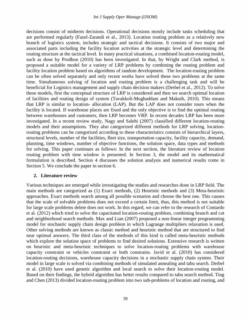
theoretical researches and practical applications in the last 20 years (Prodhon, 2010). Table 1 shows

an example of the work done in this context. Time windows for servicing are often encountered in

Logistic practical problems so that each customer must be served in her/his own time window. Sexton

and Choi(1986) were first to introduce time window into their model. Considering time window is

strictly dependent on the customer satisfaction rate so that if a customer service is delayed compared

to his/her desired time, it will lead to his/her dissatisfaction. Although this deviation from time

window does not often cause any monetary penalty, fluctuations of customer satisfaction leads to

damaging the benefits in the long term. In the conducted studies, the time window has often been

considered certain. Fazel-Zarandi et al. (2011) consider a capacitated vehicle location-routing

problem using fuzzy transportation time and certain time window for supplying the customers'

demands. What has to be taken into account regarding time window, is that the customer may

demand time window less than what is needed, or that satisfying all time windows lead to

inflexibility or ineffability of solution. Therefore, this problem is absolutely dependent on customer

behavior and, random events. Therefore, the time window is highly uncertain, stochastic and

associated with human emotion. For example, given time by a customer may be expressed in the form

of phrases like "about 9 o'clock". This approximation and lack of adequate information has led that

we use fuzzy logic to formulate time windows in the model. This theory was first suggested by Zadeh

(1965). Paper by Wang & Wan (2002) is the first study written regarding routing network using fuzzy

theory for postman problem with taking into account the time windows. In the studies done, applying

fuzzy time window to model vehicle location-routing has not been widely addressed and only Fazel

Zarandi et al. (2013) have attempted to model and solve this problem. That is why there is a need for

further research on this field. This research having considered the model in an uncertain situation has

taken into account travel time and demand and presents fuzzy variables in validity situation. This

study aims at, based on the failure experienced during solving the model, minimizing the total cost of

travel package and the facility location and also minimizing the extra travel distance. This extra

distance happens when the vehicle fails on serving some customers while on its route. The current

study intends to increase customer satisfaction in services, based on the fuzzy demands of the

customers while trying to minimize the costs. What makes this paper different from other studies in

this field is that it attempts at making the conditions more real for vehicle location-routing problem in

model. What is worthy of note here is the high-traffic routes while offering services and distributing

the products to the customers in certain times of the day. This fact causes some problems in offering

services to the customers in requested time windows that causes delay in offering those services and

finally leads to customer satisfaction. It also brings about difficulties in unloading. On the other hand,

extra costs (time and fuel consumption) are imposed to the system. Therefore, suggesting a solution


41

in this regard can influence product distribution so that it can be designed in a more appropriate

approach and prevent extra costs and customer dissatisfaction. Hence, the current study investigates

vehicle capacitated location-routing problem in fuzzy demand situation via taking into account fuzzy

time window in order to offer services to the customers and through looking at the traffic density of

the transportation routes. We did not find any study dealing with this important issue in the literature.

Table 1. Overview of the work done in the logistics field with regard to time window

Style of problem Solution Method

VRPSTW GLNPSO-EP

VRPFTW A two-stage algorithm

VRPTW Goal programming and genetic

algorithms

VRPSSTW Generated column

VRPTW Goal programming

VRPTW genetic algorithms and DEA

VRPTW tabu search

VRPTW Hybrid intelligent algorithms (fuzzy

simulation and genetic)

LRPTW Integer programming

LRPFTW Simulated annealing

3. Mathematical models

The model presented in this paper, offers a solution for the location - routing problem with fuzzy time

window and includes objectives such as minimizing total costs and maximizing customer satisfaction

level. It is assumed that the capacity of each vehicle and each customer's demand is constant and

known. Each vehicle route starts from the distribution center and ends at supply centers. Travel time

is considered to be uncertain and fuzzy. Vehicles are the same and each customer only receives

service (delete serves) from one vehicle. Only one warehouse provides all services of one client

requests.

3.1. Level of customer satisfaction

In the traditional time windows, each client request must be met in the specified time frame. So if the

customer is serviced in specified time frame it will be acceptable and the satisfaction level is good but

customer satisfaction levels with minimal distortion of time window is reduced to zero in these cases.


42

This is known as a classic and binary definition of time window that are known as crisp time window.

However, in real life, a small deviation of time window is accepted and the level of customer

satisfaction is not zero in these cases. Thus for a certain time window, two following concepts are

introduced for each client (Xu et al., 2011).

Endurable earliness time (EET): the earliest service time that a customer can endure when a service

starts earlier than e.

Endurable lateness time (ELT): the latest service time that a customer can endure when a service

starts later than l.

In this case, we have formed a fuzzy window. A diagram of such time windows is shown in Figure 1.

In this figure, parameters e and l are limits of crisp time window that provides the highest utility for

the customer.

Figure 1. outline window fuzzy

So, in this case, the customer satisfaction levels is not good and bad (0 or 1) and depending on time of

service gets the values between zero and one.

( )

{

}

Where

is a non-descending (Ascending) function of t with values between zero and one and

is descending function of t. The utility level of service can be described at various service times

using function ( ).

3.2.The traffic density in solving the model

In a network with multiple customers and multiple routes, traffic load is not distributed uniformly.

Accordingly, at one time, some of the routes are crowded, and the traffic is low in the other routes. In

this study, to avoid servicing at the traffic time, for certain customers who are located in traffic

routes, special time windows are considered that it will prevent providing the service for customer at

traffic time. This time window is defined in the interval[ ] where G and GG are beginning and


43

end of the traffic time in the traffic route. These times can be provided by traffic police and traffic

control centers. In this model, N is the node set that contains: i = 1, .., m potential warehouses and j =

m +1, ..., n customers. There is a transportation cost between the nodes (i, j) that is so that = .

Warehouse i has a capacity equal to and is the demand of customer j. The number of vehicles is

limited to k and the capacity of each one is . ̃ is travel time between two nodes i and j that are

considered as the triangular fuzzy numbers and we assume ̃ = ̃ . is the servicing time of node j

when the tour is obtained. [ ] is fuzzy time window of each customer. The goals

include: increasing levels of customer satisfaction and minimizing the total cost. The total cost

includes the warehouse cost ( ), transportation cost ( ) and the vehicle fixed costs that are

associated with each warehouse ( ). In this problem, the number of customers is M. Variable is a

binary variable associate with the warehouse i where its value is equal to one if the warehouse i has

been used otherwise it is zero. Variables associated with connecting node i to j with vehicle k, is .

If there is a connection between two nodes i and j then its value is equal one and it is zero otherwise.

Finally, if warehouse i is connected to customer j then variable is one otherwise it is zero. Based on

what was mentioned, the problem is formulated as follows. In this model, function (1) is used for

maximizing the satisfaction level of each client. The constraint (12), (13) and (14) are used to

consider nonlinear objective function (1) in the model consequently the linear objective function (3)

has been obtained.

(1) ( (

))

Objective functions:

∑ ∑ ∑ ∑ ∑ ∑ ∑ (2)

(3)

(∑ )

Constraints of the model are as follows:

(4) ∑ ∑

(5) ∑ ∑

(6) ∑

(7) ∑ ∑

(8) ∑ ∑

(9) ∑ ∑ | |

(10) ∑ ∑ { }

(11) ∑ ∑ ( ̃ )

(12) ( ) ( ))


44

(13) (( ) ( ))

(14)

(15)

(16) ( ) ( )

(17) { }

(18) { }

(19) { }

{ } (20)

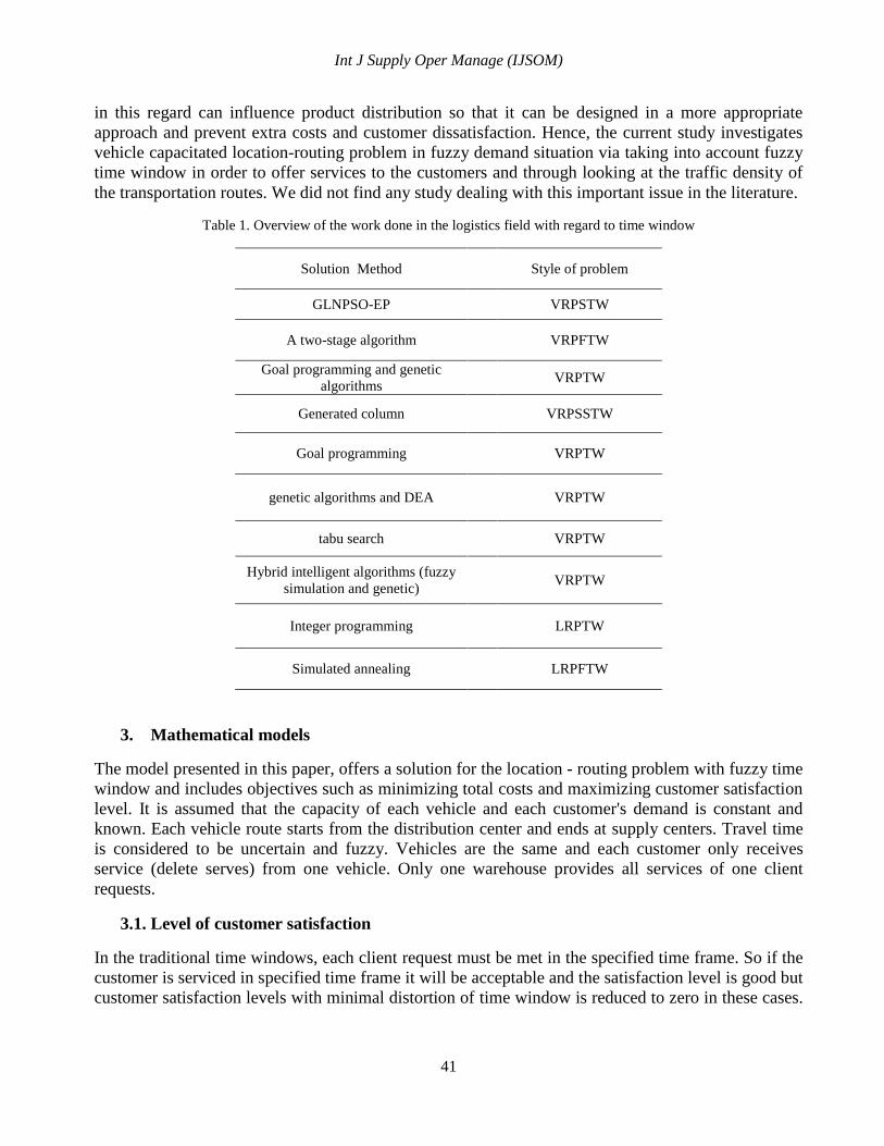
In the mathematical model, equation (2) represents the first objective function which minimizes the

transportation total cost and the warehouses construction cost. In this regard, the total cost includes of

(delete) the warehouse cost, the vehicle fixed cost, the transportation cost from one node to another

node and resulted penalty cost from exposure to the time window of traffic routes. The second

objective function, equation (3), maximizes average of customer satisfaction level. Equation (4)

denotes that each customer is assigned to only one route. Equation (5) expresses that the total

customer demand on a route does not exceed the vehicle capacity. Equation (6) denotes that the total

goods supplied from any used warehouse should not exceed its capacity. Equation (7) expresses that

if a vehicle entered into each node, then it must exit from that node. Equation (8) denotes that a

customer demand is supplied from a one (delete) warehouse. Equation (9) is added to omit sub tour

where S is a subset of the customer nodes. Equation (10) ensures that the client must be connected to

the warehouse if there is a path between them. This constraint implies that the vehicle which exits

from the warehouse, then it comes back to it. Equation (11) expressed the vehicle's arrival time to

each customer according to the tour route sequence. Equations (12), (13) and (14) are added to the

model in order to consider objective function of the level of the customer satisfaction as linear

function. Equation (15) is based on the sequence selection where the service time per customer's

request should be placed within the time window. Equation (16) gives a penalty to the objective

function if the vehicle is located in traffic time window. In this regard, [ ]is time window

associated with crowded Hours. Equations (17), (18), (19) and (20) indicates the decision variables

types. LRP is an NP-hard problem because it is formed of two NP-hard problems (location of

facilities and vehicle routing) (Fazel-Zarandi et al., 2011). Therefore exact methods cannot be

effective for solving large problems and heuristic and Meta-heuristic methods must be used to solve.

A genetic algorithm (GA) is used in order to solve the proposed model. Therefore, due to the

dependence of the minimum and maximum values simultaneously and the requirement to use near

optimal solution, techniques such as multi-objective utility function (MAUT) or methods of fuzzy

programming do not seem to be suitable for converting multiple objectives into a single one. We

investigated methods such as multi-objective utility function and it is observed that its consequences

did not show good convergence process. Therefore, the weighted sum method is used to integrate the

objective functions. This method is so easy to understand for decision maker and allow him to

examine the objectives based on the targets importance by giving different weight to each one.


45

Therefore, is defined as the weight for objective i. Conflicting goals can be aligned with a

negative coefficient.

(21) ( ) ∑ ( ( ))

4. Genetic Algorithm

Due to the nature of NP-hard problem, one approach for problem solving is to use Meta-heuristics

algorithms, thus, genetic algorithm has been chosen to solve the proposed model. Genetic algorithm

is a powerful algorithm for solving optimization problems and engineering designs (Stanciulescu et

al., 2003). In this paper, first we present a simulated algorithm for calculation purposes then solution

structure in terms of genetic algorithms for solving the location - routing problem with fuzzy time

windows and traffic hours is described.

4.1.The proposed algorithm for solving the model

Since the travel time between the warehouse and the customer is uncertain, the triangular fuzzy

numbers are defuzzified, in order to transform the fuzzy problem into an equivalent crisp problem.

This method is summarized as follows according to Fazel Zarandi et al. (2013). For each customer, a

number t is generated in the interval between upper and lower limit of triangular fuzzy numbers. Next

a random number is generated in the range of zero and one. λ is the membership function for value

of t. As long as, λ is smaller than random number , Then the value of t and λ will be accepted. In the

other words, when β 𝛌 then value of t is reported as the simulation time. Other steps of algorithm

are as follows,

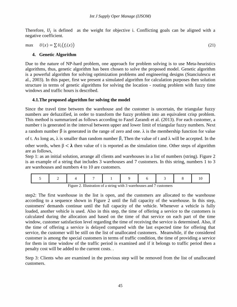
Step 1: as an initial solution, arrange all clients and warehouses in a list of numbers (string). Figure 2

is an example of a string that includes 3 warehouses and 7 customers. In this string, numbers 1 to 3

are warehouses and numbers 4 to 10 are customers.

10 8 3 6 9 1 7 4 2 5

Figure 2. Illustration of a string with 3 warehouses and 7 customers

step2: The first warehouse in the list is open, and the customers are allocated to the warehouse

according to a sequence shown in Figure 2 until the full capacity of the warehouse. In this step,

customers' demands continue until the full capacity of the vehicle. Whenever a vehicle is fully

loaded, another vehicle is used. Also in this step, the time of offering a service to the customers is

calculated during the allocation and based on the time of that service on each part of the time

window, customer satisfaction level regarding the time of receiving the service is determined. Also, if

the time of offering a service is delayed compared with the last expected time for offering that

service, the customer will be still on the list of unallocated customers. Meanwhile, if the considered

customer is among the special customers in terms of traffic condition, the time of providing a service

for them in time window of the traffic period is examined and if it belongs to traffic period then a

penalty cost will be added to the current costs. .

Step 3: Clients who are examined in the previous step will be removed from the list of unallocated

customers.


46

Step 4: If warehouse capacity constraint is violated, the warehouse will be removed from the initial

list. In this case, Return to step 2 again, and the remaining unallocated clients are assigned to the next

warehouse.

Step 5: If any client is still remained from the primary list back to step 2.

Step 6: with allocating all clients, the algorithm finishes.

4.1.1. Genetic Algorithm

Step 1: Initial population generation: a genetic algorithm starts with an initial population of solutions.

Each solution is displayed by a chromosome that is a string of bits. All possible solutions should be

displayed using a coding system.

Step 2: Determine the fitness value after the customer's allocation to warehouses, according to

mentioned steps in the proposed algorithm, the fitness level of each chromosome is determined.

Step 3: Populations Generating

Selection: The first step involves selecting parent from population for generation of new solutions.

This chosen selection is done randomly with regards to a probability that is proportional to their

fitness function. At this stage, it should be decided about how to select parents for crossover

operation, how to generate offspring and numbers of children. Parents are often chosen by using

roulette wheel method. In this paper, we used this method too.

Generation: In the second step, Recombination and mutation operators on selected individuals are

used and new chromosomes are generated.

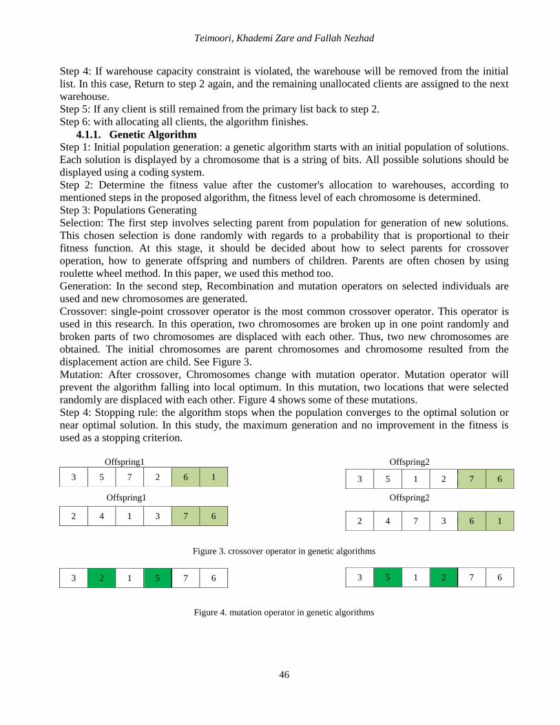
Crossover: single-point crossover operator is the most common crossover operator. This operator is

used in this research. In this operation, two chromosomes are broken up in one point randomly and

broken parts of two chromosomes are displaced with each other. Thus, two new chromosomes are

obtained. The initial chromosomes are parent chromosomes and chromosome resulted from the

displacement action are child. See Figure 3.

Mutation: After crossover, Chromosomes change with mutation operator. Mutation operator will

prevent the algorithm falling into local optimum. In this mutation, two locations that were selected

randomly are displaced with each other. Figure 4 shows some of these mutations.

Step 4: Stopping rule: the algorithm stops when the population converges to the optimal solution or

near optimal solution. In this study, the maximum generation and no improvement in the fitness is

used as a stopping criterion.

Offspring1 Offspring2

Offspring1 Offspring2

Figure 3. crossover operator in genetic algorithms

Figure 4. mutation operator in genetic algorithms

1 6 2 7 5 3 6 7 2 1 5 3

6 7 3 1 4 2 1 6 3 7 4 2

6 7 2 1 5 3 6 7 5 1 2 3


47

5. Numerical results

In this section, we present an example to elaborate how the algorithm works. In this example, 4

warehouses are potentially intended to serve 15 clients; the warehouses have different costs and

different capacities. Warehouses are numbered with number 1 to 4 and clients are denoted with the

numbers 5 to 19. Transportation time between each clients and their warehouses are in the form of

triangular fuzzy numbers (a, b, c), are shown in Table 2. Table 3 shows the transportation cost

between the clients and warehouse. Clients demand and time window for servicing clients are shown

by trapezoidal fuzzy numbers ( ) which are presented in Table 4. The

capacity of each vehicle is 600 units. In this example, for the customers with number of 5, 7,

8,11,12,15 and 17, traffic time interval is defined. If the vehicle enters in this time interval, then we

are faced with 1,000 unit penalty cost. The data used in this study, has been adapted from (Zheng and

Liu, (2006)), but customer time window and traffic time windows are added to this example. The

program was codified using Matlab and was run in a 2-GIG memory PC. The results (with 100 ring

repetitions and 100 production sequences as chromosome in each ring) exhibit the optimal plan for

vehicles' mobility as below. The results show that optimized design for moving vehicles is as follows.

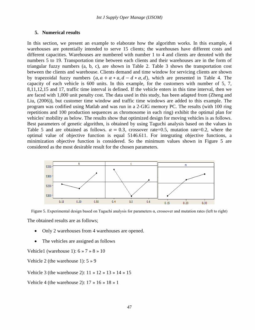
Best parameters of genetic algorithm, is obtained by using Taguchi analysis based on the values in

Table 5 and are obtained as follows. , crossover rate=0.5, mutation rate=0.2, where the

optimal value of objective function is equal 5146.611. For integrating objective functions, a

minimization objective function is considered. So the minimum values shown in Figure 5 are

considered as the most desirable result for the chosen parameters.

Figure 5. Experimental design based on Taguchi analysis for parameters α, crossover and mutation rates (left to right)

The obtained results are as follows;

Only 2 warehouses from 4 warehouses are opened.

The vehicles are assigned as follows

Vehicle1 (warehouse 1): 6 » 7 » 8 » 10

Vehicle 2 (the warehouse 1): 5 » 9

Vehicle 3 (the warehouse 2): 11 » 12 » 13 » 14 » 15

Vehicle 4 (the warehouse 2): 17 » 16 » 18 » 1


48

Table 2. Transportation time matrix

7 6 5 4 3 2 Number 1

1

2 (5, 10, 15)

3 (25, 50, 75) (5, 10, 15)

4 (7, 15, 23) (25, 50, 75) (7, 15, 23)

5 (25, 50, 75) (17, 35, 53) (17, 35, 53) (15, 30, 45)

6 (25, 50, 75) (7, 15, 23) (20, 40, 60) (2, 5, 8) (22, 45, 68)

7 (12, 25, 38) (20, 40, 60) (15, 30, 45) (17, 35, 53) (7, 15, 23) (12, 25, 38)

8 (7, 15, 23) (20, 40, 60) (5, 10, 15) (22, 45, 68) (10, 20, 30) (17, 35, 53) (20, 40, 60)

9 (25, 50, 75) (7, 15, 23) (22, 45, 68) (5, 10, 15) (22, 45, 68) (15, 30, 45) (5, 10, 15)

10 (10, 20, 30) (22, 45, 68) (12, 25, 38) (22, 45, 68) (7, 15, 23) (15, 30, 45) (20, 40, 60)

11 (25, 50, 75) (5, 10, 15) (17, 35, 53) (15, 30, 45) (17, 35, 53) (5, 10, 15) (15, 30, 45)

12 (27, 55, 83) (17, 35, 53) (17, 35, 53) (15, 30, 45) (17, 35, 53) (2, 5, 8) (15, 30, 45)

13 (5, 10, 15) (20, 40, 60) (5, 10, 15) (20, 40, 60) (7, 15, 23) (15, 30, 45) (17, 35, 53)

14 (25, 50, 75) (5, 10, 15) (20, 40, 60) (2, 5, 8) (22, 45, 68) (15, 30, 45) (2, 5, 8)

15 (22, 45, 68) (5, 10, 15) (20, 40, 60) (5, 10, 15) (22, 45, 68) (15, 30, 45) (5, 10, 15)

16 (7, 15, 23) (22, 45, 68) (7, 15, 23) (22, 45, 68) (10, 20, 30) (15, 30, 45) (22, 45, 68)

17 (15, 30, 45) (20, 40, 60) (12, 25, 38) (20, 40, 60) (10, 20, 30) (12, 25, 38) (17, 35, 53)

18 (25, 50, 75) (5, 10, 15) (22, 45, 68) (5, 10, 15) (25, 50, 75) (15, 30, 45) (7, 15, 23)

19 (25, 50, 75) (20, 40, 60) (20, 40, 60) (22, 45, 68) (17, 35, 53) (15, 30, 45) (17, 35, 53)

14 13 12 11 10 9 8

8

9 (20, 40, 60)

10 (5, 10, 15) (12, 25, 38)

11 (5, 10, 15) (17, 35, 53) (17, 35, 53)

12 (7, 15, 23) (17, 35, 53) (17, 35, 53) (12, 25, 38)

13 (17, 35, 53) (5, 10, 15) (20, 40, 60) (20, 40, 60) (17, 35, 53)

14 (17, 35, 53) (17, 35, 53) (5, 10, 15) (20, 40, 60) (15, 30, 45) (15, 30, 45)

15 (17, 35, 53) (17, 35, 53) (2, 5, 8) (20, 40, 60) (15, 30, 45) (20, 40, 60) (20, 40, 60)

16 (17, 35, 53) (10, 20, 30) (22, 45, 68) (15, 30, 45) (17, 35, 53) (7, 15, 23) (7, 15, 23)

17 (2, 5, 8) (12, 25, 38) (20, 40, 60) (5, 10, 15) (12, 25, 38) (12, 25, 38) (12, 25, 38)

18 (17, 35, 53) (20, 40, 60) (7, 15, 23) (20, 40, 60) (15, 30, 45) (20, 40, 60) (20, 40, 60)

19 (17, 35, 53) (20, 40, 60) (22, 45, 68) (15, 30, 45) (7, 15, 23) (17, 35, 53) (20, 40, 60)

19 18 17 16 15

15

16 (22, 45, 68)

17 (17, 35, 53) (17, 35, 53)

18 (7, 15, 23) (7, 15, 23) (20, 40, 60)

19 (2, 5, 8) (22, 45, 68) (12, 25, 38) (20, 40, 60)


49

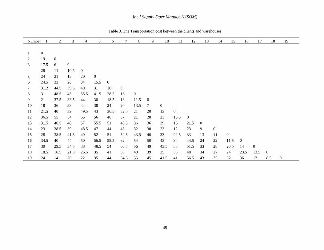
Table 3. The Transportation cost between the clients and warehouses

Number 1 2 3 4 5 6 7 8 9 10 11 12 13 14 15 16 17 18 19

1 0

2 19 0

3 17.5 6 0

4 28 11 10.5 0

5

6

24 21 15 20 0

24.5 32 26 34 15.5 0

7 31.2 44.5 39.5 49 31 16 0

8 31 48.5 45 55.5 41.5 28.5 16 0

9 21 37.5 33.5 44 30 18.5 13 11.5 0

10 18 36 33 44 38 24 20 13.5 7 0

11 21.5 40 39 49.5 43 36.5 32.5 21 20 13 0

12 36.5 55 54 65 56 46 37 21 28 23 15.5 0

13 31.5 46.5 48 57 55.5 51 48.5 36 36 29 16 21.5 0

14 23 38.5 39 48.5 47 44 43 32 30 23 12 23 9 0

15 28 38.5 41.5 49 52 51 52.5 43.5 40 33 22.5 33 13 11 0

16 34.5 40 44 50 56.5 58.5 62 54 50 43 34 44.5 24 22 11.5 0

17 30 29.5 34.5 38 48.5 54 60.5 56 49 43.5 38 51.5 33 28 20.5 14 0

18 18.5 16.5 21.3 26.5 35 41 50 48 39 35 33 48 34 27 24 23.5 13.5 0

19 24 14 20 22 35 44 54.5 55 45 41.5 41 56.5 43 35 32 36 17 8.5 0


50

Table 4. Demand, expected time window, and the customer traffic time interval

number demand expected time window Traffic

interval

number demand expected time window Traffic

interval

5 160 [9:22, 11:09, 12:05,

12:17]

[9:40, 10:10] 13 200 [9:15, 9:19, 10:59, 11:50]

6 200 [9:12, 9:15, 11:09, 12.05] 14 80 [9:12, 9:15, 11:09, 12.05]

7 60 [9:12, 9:15, 11:09, 12.05] [9:20, 9:50] 15 60 [9:12, 9:15, 11:04, 11.57] [10:50, 11:25]

8 200 [9:12, 9:15, 10:59, 11.50] [9:18, 9:45] 16 200 [9:12, 9:15, 11:04, 11.57]

9 135 [9:13, 9:16, 11:04, 11:57] 17 90 [9:12, 9:15, 11:38, 12.47] [10:25, 10:40]

10 120 [9:12, 9:15, 11:09, 12.05] 18 200 [9:15, 9:19, 11:09, 12:05]

11 140 [9:15, 9:19, 10:04, 11:57] [9:30, 10:00] 19 100 [9:15, 9:19, 11:02, 11:55]

12 100 [9:12, 9:15, 11:15, 12.13] [10:10, 10:35]

Based on the above sequence, the customer service time in each tour is as follows

Vehicle1 (warehouse 1): 35 » 62 » 85 » 94

Vehicle 2 (the warehouse 1): 38 » 65

Vehicle 3 (the warehouse 2): 6 » 23 » 43 » 61 » 82

Vehicle 4 (the warehouse 2): 15 » 36 » 46 » 75

We Assume, the start time of the service is 9 am, which is equal to 0. So the results show that

customer service times are not in traffic hours.

6. Results Validation

In order to validate the results, we show that how our robust algorithm works by using various

algorithm parameters.

Table 5 shows sensitivity analysis results on various parameters used in the model. In this Table, represents the crossover rate, represent mutation rate and α represents the change percentage in

the range of customer's time window used in trapezoidal fuzzy numbers( ). Based on different values for above parameters, optimum solution has been reported. Finally, error

terms are reported. The amount of percent error is obtained from following equation.


51

The results show that the deviation percentage of objective function doesn't exceed than 4.5 percent.

This shows that model has credibility and stability in the different situations. The proposed approach

is effective to solve the problem considered in this paper.

Table 5. Results comparison with different values of the problem parameters.

error Function

value α pop size

0.022751 5279.16 0.6 0.2 0.15 100

0.023407 5282.505 0.4 0.15 0.15 100

0.009651 5211.5 0.5 0.3 0.15 100

0.020816 5269.129 0.5 0.2 0.3 100

0.034844 5341.54 0.4 0.3 0.3 100

0 5161.685 0.6 0.15 0.3 100

0.045559 5396.845 0.6 0.3 0.5 100

0.041872 5377.814 0.4 0.2 0.5 100

0.001651 5170.208 0.5 0.15 0.5 100

7. Conclusion

In this paper, we provided a location-routing model with fuzzy time windows in terms of travel time

uncertainty with regard to traffic restrictions on congested routes. A genetic algorithm is used to

solve the model. Model results are illustrated by a numerical example. The sensitivity of the

optimum solution has been investigated by changing parameters affecting on the model. As future

researches, the transportation time and demand may be considered to be non-deterministic. Also

using other meta-heuristics algorithm is also suggested as future researches. It also obtained

transportation costs in a more real form and based on the inflation rates and fluctuations in fuel

price, considered reopening the warehouses taking into account its future benefits in the model.

This study has considered traffic routes and times, so the research results can be applied in urban

transportation system which the traffic routes and times are important parts of it.

References

Ahmadi Javid A. and Azad N. (2010). Incorporating location, routing and inventory decisions in

supply chain network design , Transportation Research Part E. Vol. 46, pp. 582–597.

Caballero R., Gonzalez M., Ma Guerrero F., Molina J. and Paralera C. (2007). Solving a multi

objective location routing problem with a meta-heuristic based on Tabu search. Application to a real

case in Andalusia, European Journal of Operational Research, Vol. 177, pp. 1751–1763.


52

Claudio C., Vera H. and Teodor G.C. (2012). Lower and upper bounds for the two-echelon

capacitated location-routing problem. Computers & Operations Research, Vol. 39, pp. 3185–3199.

Contardo C., Hemmelmayr V. and Gabriel-Crainic T. (2012). Lower and upper bounds for the two-

echelon capacitated location-routing problem. Computers & Operations Research, Vol. 39, pp.

3185–3199.

Derbel H., Jarboui B., Hanafi S. and Chabchoub H. (2010). An Iterated Local Search for Solving A

Location-Routing Problem. Electronic Notes in Discrete Mathematics, Vol. 36, pp. 875–882.

Derbel H., Jarboui B., Hanafi S. and Chabchoub H. (2012). Genetic algorithm with iterated local

search for solving a location-routing problem. Expert Systems with Applications, Vol. 39, pp. 2865–

2871.

Fazel-Zarandi M.H., Hemmati A., Davari S. and Turksen B. (2013). Capacitated location-routing

problem with time windows under uncertainty. Knowledge-Based Systems, Vol. 37, pp. 480–489.

Fazel-Zarandi M.H., Hemmati A. and Davari S. (2011). The multi-depot capacitated location-

routing problem with fuzzy travel times. Expert Systems with Applications, Vol. 38, pp. 10075–

10084.

Homberger J. and Gehring H. (2005). A two-phase hybrid meta-heuristic for the vehicle routing

problem with time windows. European Journal of Operational Research, Vol. 162, pp. 220–238.

Jabal-Ameli M.S. Ghaffari-Nasab N. (2010). Location Routing Problem with Time Window. Novel

mathematicalprogramming formulations, 7th international Industrial engineering conference,

Isfahan. Iran.

Lau H.C.W. and Jiang Z.Z. and Ip W.H. and Wang D. (2010). A credibility-based fuzzy location

model with Hurwicz criteria for the design of distribution systems in B2C e-commerce. Computers

& Industrial Engineering, Vol. 59, pp.873–886.

Lin C.K.Y. and Kwok R.C.W. (2006). Multi-objective meta-heuristics for a location-routing

problem with multiple use of vehicles on real data and simulated data. European Journal of

Operational Research, Vol. 175, pp. 1833–1849.

Max S.Z.J., Lian Q. (2007). Incorporating inventory and routing costs in strategic location models.

European Journal of Operational Research, Vol. 179, pp. 372–389.

Nagy G. and Salhi S. (2007). Location-routing: Issues, models and methods. European Journal of

Operational Research, Vol. 177, pp. 649–672.

Prodhon C. (2010). A hybrid evolutionary algorithm for the periodic location-routing problem.

European Journal of Operational Research, Vol. 210, pp. 204–212.


53

Sexton T. and Choi Y. (1986). Pickup and delivery of partial loads with soft time windows.

American Journal of Mathematical and Management, Vol. 6, pp. 369–398.

Sibel A. and Kara-Bahar Y. (2007). A new model for the hazardous waste location-routing problem.

Computers & Operations Research, Vol. 34, pp. 1406–1423.

Stanciulescu C., Fortemps P., Install M. and Wertz V. (2003). Multi objective fuzzy linear

programming problems with fuzzy decision variables. European Journal of Operational Research,

Vol. 149, pp. 654–675.

Stenger A., Schneider M., Schwind M. and Vigo D. (2012). Location routing for small package

shippers with subcontracting options. International Journal of Production Economics, Vol. 140(2),

pp. 702–712.

Tang J., Pana Z., Fung R. and Lau H. (2009). Vehicle routing problem with fuzzy time windows.

Fuzzy Sets and Systems, Vol. 160, pp. 683–695.

Tavakkoli-Moghaddam A. and Makuib M. (2010). A new integrated mathematical model for a bi-

objective multi-depot location-routing problem solved by a multi-objective scatter search algorithm.

Journal of Manufacturing Systems, Vol. 29, pp. 111–119.

Ting C.J. and Chen C.H. (2013). A multiple ant colony optimization algorithm for the capacitated

location routing problem. International Journal of Production Economics, Vol. 141(1), pp. 34-44.

Wang H.F. and Wen Y.P. (2002). Time-constrained Chinese postman problems, Comput. Math. Vol.

44, pp. 375–387.

Xie Y., Lu W., Wangb W. and Quadrifogliob L. (2012). A multimodal location and routing model

for hazardous materials transportation. Journal of Hazardous Materials, Vol. 227– 228, pp.135–

141.

Xu J., Yan F. and Li S. (2011). Vehicle routing optimization with soft time windows in a fuzzy

random environment. Transportation Research Part E, Vol. 47, pp. 1075–1091.

Yu V.F., Lin S.W., Lee W. and Ting C.J. (2010). A simulated annealing heuristic for the capacitated

location routing problem. Computers & Industrial Engineering, Vol. 58, pp. 288–299.

Zadeh, L. (1965). Fuzzy sets. Information and Control, Vol. 8, pp. 338–353.

Zheng Y. and Liu B. (2006). Fuzzy vehicle routing model with credibility measure and its hybrid

intelligent algorithm. Applied Mathematics and Computation, Vol. 176, pp. 673–683.