ECE 2610 Signal and Systems 8–1 IIR Filters In this chapter we finally study the general infinite impulse response (IIR) difference equation that was men- tioned back in Chapter 5. The filters will now include both feed- back and feedforward terms. The system function will be a rational function where in general both the zeros and the poles are at nonzero locations in the z-plane. The General IIR Difference Equation • The general IIR difference equation described in Chapter 5 was of the form (8.1) • In this chapter the text rearranges this equation so that is on the left and all of the other terms are on the right (8.2) • In so doing notice the sign change of the coefficients, and also we assume that • The total coefficient count is , meaning that this many multiplies are needed to compute each new output from the difference equation a l yn l – l 0 = N b k xn k – k 0 = M = yn yn a l yn l – l 1 = N b k xn k – k 0 = M + = a l a 0 1 = N M 1 + + Chapter 8

Welcome message from author
This document is posted to help you gain knowledge. Please leave a comment to let me know what you think about it! Share it to your friends and learn new things together.
Transcript
er
IIR FiltersIn this chapter we finally study the general infiniteimpulse response (IIR) difference equation that was men-tioned back in Chapter 5. The filters will now include both feed-back and feedforward terms. The system function will be arational function where in general both the zeros and the polesare at nonzero locations in the z-plane.The General IIR Difference Equation
• The general IIR difference equation described in Chapter 5was of the form
(8.1)
• In this chapter the text rearranges this equation so that ison the left and all of the other terms are on the right
(8.2)
• In so doing notice the sign change of the coefficients,and also we assume that
• The total coefficient count is , meaning that thismany multiplies are needed to compute each new output fromthe difference equation
al y n l– l 0=
N
bk x n k– k 0=
M
=
y n
y n al y n l– l 1=
N
bk x n k– k 0=
M
+=
al a0 1=
N M 1+ +
Chapt
8
ECE 2610 Signal and Systems 8–1
Time-Domain Response
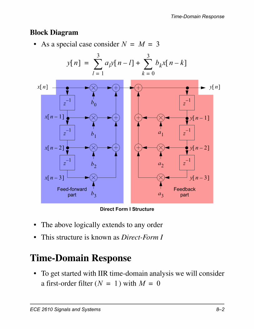
Block Diagram
• As a special case consider
• The above logically extends to any order
• This structure is known as Direct-Form I
Time-Domain Response
• To get started with IIR time-domain analysis we will considera first-order filter ( ) with
N M 3= =
y n aly n l– l 1=
3
bkx n k– k 0=
3
+=
y n x n
z1–
z1–
z1–
z1–
z1–
z1–
y n 1–
y n 2–
y n 3–
x n 1–
x n 2–
x n 3–
b0
b1
b2
b3
a1
a2
a3Feed-forward
partFeedback
part
Direct Form I Structure
N 1= M 0=
ECE 2610 Signals and Systems 8–2

Time-Domain Response
(8.3)
Impulse Response of a First-Order IIR System
• The impulse response can be obtained by setting and insuring that the system is initially at rest
• Definition: Initial rest conditions for an IIR filter means that:
– (1) The input is zero prior to the start time , that is for
– (2) The output is zero prior to the start time, that is for
• We now proceed to find the impulse response of (8.3) viadirect recursion of the difference equation
• In summary we have shown that the impulse response of a1st-order IIR filter is
(8.4)
where the unit step has been utilized to make it clearthat the output is zero for
y n a1y n 1– b0x n +=
x n n =
n0x n 0= n n0
y n 0= n n0
y 0 a1y 1– b0 0 + b0= =
y 1 a1y 0 b0 1 + a1b0= =
y 2 a1y 1 b0 2 + a12b0= =
y n a1nb0 n 0=
0
0
0
h n b0 a1 nu n =
u n n 0
ECE 2610 Signals and Systems 8–3
Time-Domain Response
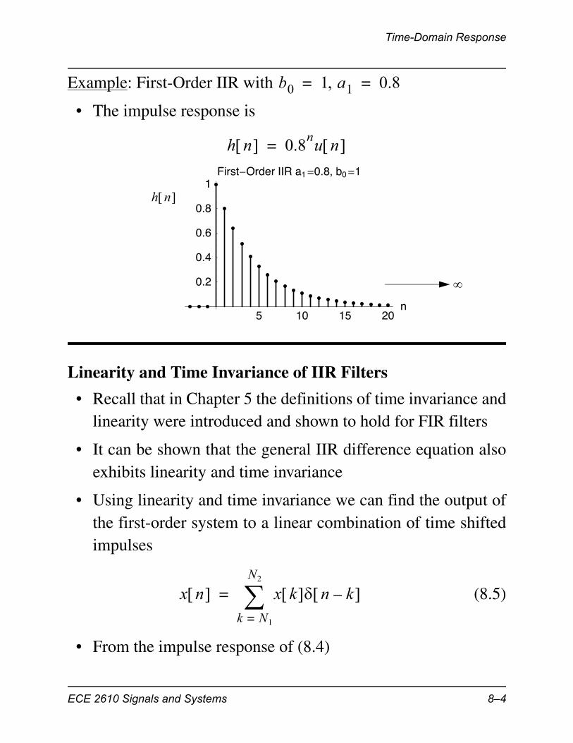
Example: First-Order IIR with
• The impulse response is
Linearity and Time Invariance of IIR Filters
• Recall that in Chapter 5 the definitions of time invariance andlinearity were introduced and shown to hold for FIR filters
• It can be shown that the general IIR difference equation alsoexhibits linearity and time invariance
• Using linearity and time invariance we can find the output ofthe first-order system to a linear combination of time shiftedimpulses
(8.5)
• From the impulse response of (8.4)
b0 1 a1 0.8= =
h n 0.8nu n =
5 10 15 20n
0.2
0.4
0.6
0.8
1First�Order IIR a1�0.8, b0�1
h n
x n x k n k– k N1=
N2
=
ECE 2610 Signals and Systems 8–4
Time-Domain Response
(8.6)
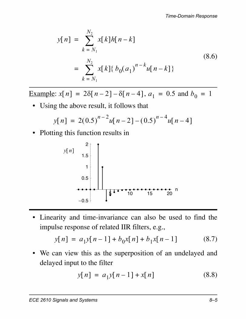
Example: , and
• Using the above result, it follows that
• Plotting this function results in
• Linearity and time-invariance can also be used to find theimpulse response of related IIR filters, e.g.,
(8.7)
• We can view this as the superposition of an undelayed anddelayed input to the filter
(8.8)
y n x k h n k– k N1=
N2
=
x k b0 a1 n k–u n k–
k N1=
N2
=
x n 2 n 2– n 4– –= a1 0.5= b0 1=
y n 2 0.5 n 2–u n 2– 0.5 n 4–
u n 4– –=
5 10 15 20n
�0.5
0.5
1
1.5
2y n
y n a1y n 1– b0x n b1x n 1– + +=
y n a1y n 1– x n +=
ECE 2610 Signals and Systems 8–5
Time-Domain Response
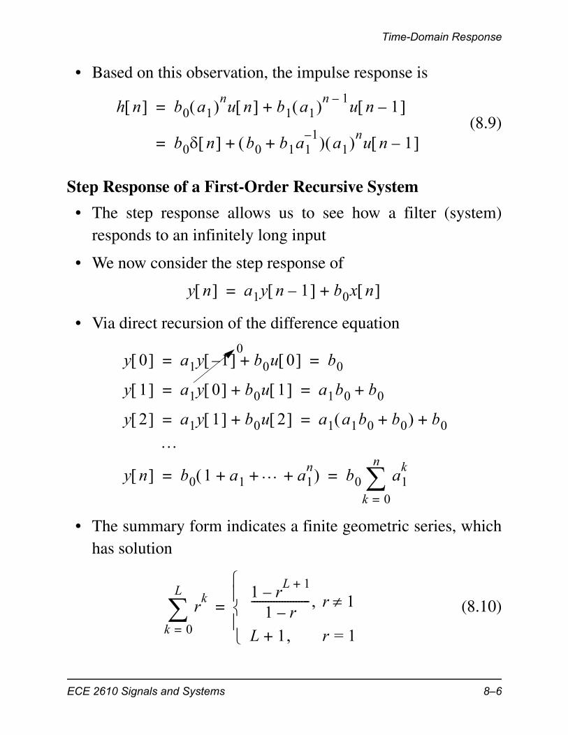
• Based on this observation, the impulse response is
(8.9)
Step Response of a First-Order Recursive System
• The step response allows us to see how a filter (system)responds to an infinitely long input
• We now consider the step response of
• Via direct recursion of the difference equation
• The summary form indicates a finite geometric series, whichhas solution
(8.10)
h n b0 a1 nu n b1 a1 n 1–u n 1– +=
b0 n b0 b1a11–
+ a1 nu n 1– +=
y n a1y n 1– b0x n +=
y 0 a1y 1– b0u 0 + b0= =
y 1 a1y 0 b0u 1 + a1b0 b0+= =
y 2 a1y 1 b0u 2 + a1 a1b0 b0+ b0+= =
y n b0 1 a1 a1
n+ + + b0 a1
k
k 0=
n
= =
0
rk
k 0=
L
1 r
L 1+–1 r–
--------------------- , r 1
L 1,+ r = 1
=
ECE 2610 Signals and Systems 8–6
Time-Domain Response
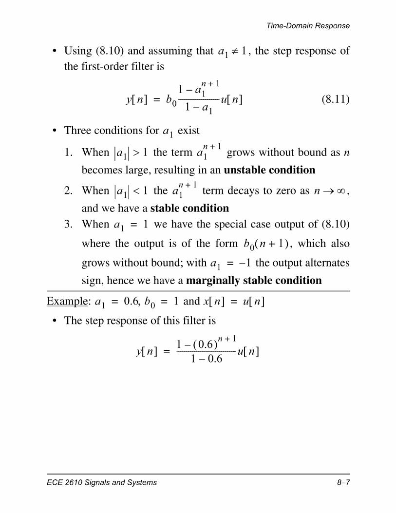
• Using (8.10) and assuming that , the step response ofthe first-order filter is
(8.11)
• Three conditions for exist
1. When the term grows without bound as n
becomes large, resulting in an unstable condition
2. When the term decays to zero as ,
and we have a stable condition3. When we have the special case output of (8.10)
where the output is of the form , which also
grows without bound; with the output alternates
sign, hence we have a marginally stable condition
Example: and
• The step response of this filter is
a1 1
y n b0
1 a1n 1+
–
1 a1–---------------------u n =
a1
a1 1 a1n 1+
a1 1 a1n 1+
n
a1 1=
b0 n 1+
a1 1–=
a1 0.6 b0 1= = x n u n =
y n 1 0.6 n 1+–1 0.6–
-------------------------------u n =
ECE 2610 Signals and Systems 8–7

Time-Domain Response
• The step response can also be obtained by direct evaluationof the convolution sum
(8.4)
• For the problem at hand
(8.5)
• To evaluate this requires careful attention to details
• The product tells us how to set the sum limits
5 10 15 20n
0.5
1
1.5
2
2.5y n
y n x n *h n u n *h n = =
y n u k b0 a1 n k–u n k–
k –=
=
u k u n k–
k
k
n 0
0
0
u n k–
u k
n 0
n n
ECE 2610 Signals and Systems 8–8
System Function of an IIR Filter
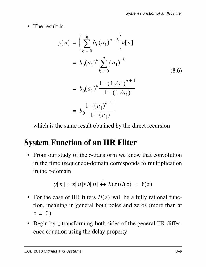
• The result is
(8.6)
which is the same result obtained by the direct recursion
System Function of an IIR Filter
• From our study of the z-transform we know that convolutionin the time (sequence)-domain corresponds to multiplicationin the z-domain
• For the case of IIR filters will be a fully rational func-tion, meaning in general both poles and zeros (more than at
)
• Begin by z-transforming both sides of the general IIR differ-ence equation using the delay property
y n b0 a1 n k–
k 0=
n
u n =
b0 a1 n a1 k–
k 0=
n
=
b0 a1 n1 1 a1 n 1+
–
1 1 a1 –------------------------------------=
b0
1 a1 n 1+–
1 a1 –-----------------------------=
y n x n *h n = X z H z Y z =z
H z
z 0=
ECE 2610 Signals and Systems 8–9
System Function of an IIR Filter
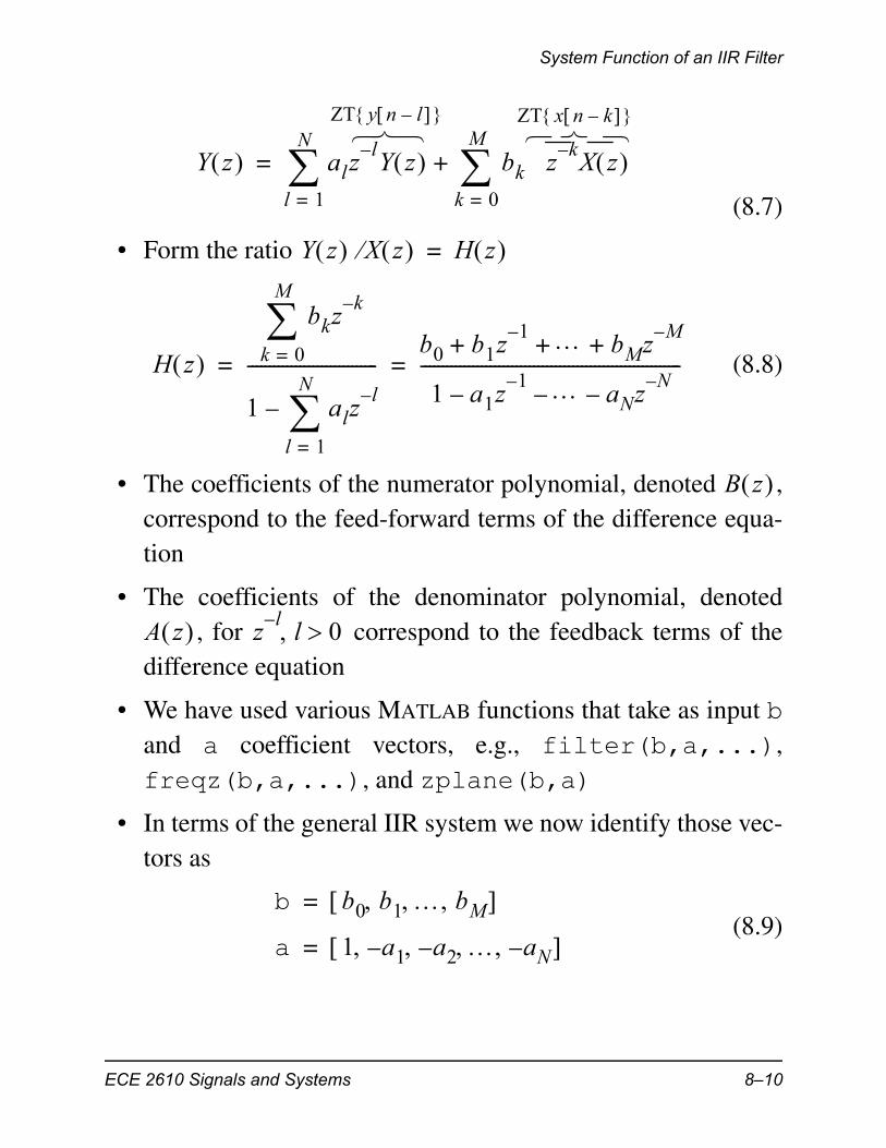
(8.7)
• Form the ratio
(8.8)
• The coefficients of the numerator polynomial, denoted ,correspond to the feed-forward terms of the difference equa-tion
• The coefficients of the denominator polynomial, denoted, for correspond to the feedback terms of the
difference equation
• We have used various MATLAB functions that take as input band a coefficient vectors, e.g., filter(b,a,...),freqz(b,a,...), and zplane(b,a)
• In terms of the general IIR system we now identify those vec-tors as
(8.9)
Y z alzl–Y z
l 1=
N
bk zk–X z
k 0=
M
+=
ZT y n l– ZT x n k–
Y z X z H z =
H z
bkzk–
k 0=
M
1 alzl–
l 1=
N
–
------------------------------b0 b1z
1– bMzM–
+ + +
1 a1z1–
– aNzN–
––------------------------------------------------------------= =
B z
A z zl–l 0
b b0 b1 bM =
a 1 a1 a2– aN– – =
ECE 2610 Signals and Systems 8–10
System Function of an IIR Filter
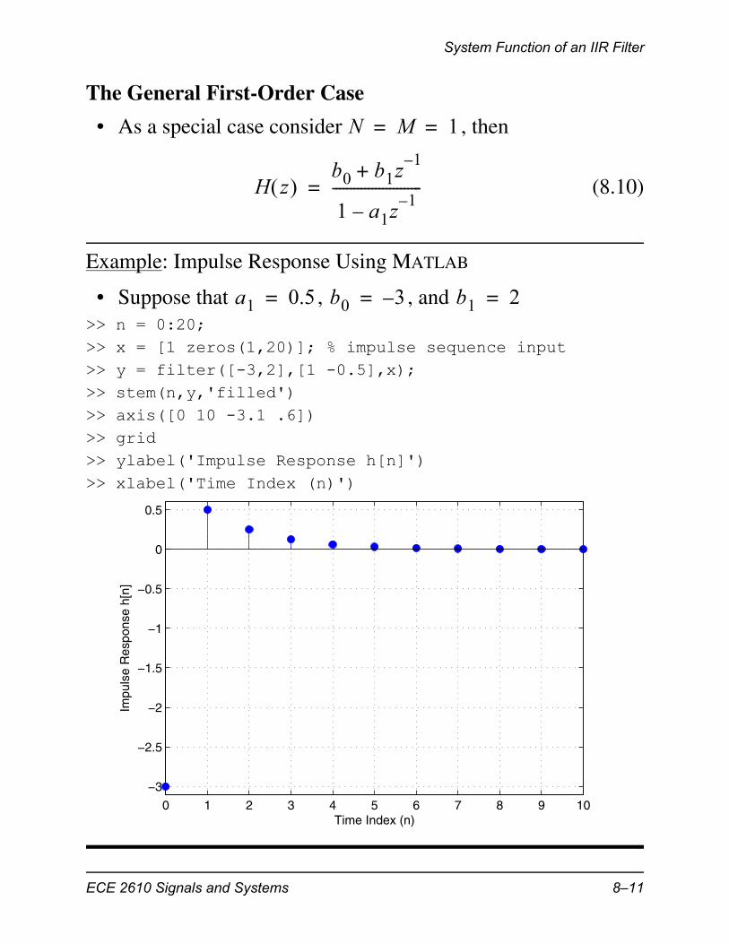
The General First-Order Case
• As a special case consider , then
(8.10)
Example: Impulse Response Using MATLAB
• Suppose that , , and >> n = 0:20;>> x = [1 zeros(1,20)]; % impulse sequence input>> y = filter([-3,2],[1 -0.5],x);>> stem(n,y,'filled')>> axis([0 10 -3.1 .6])>> grid>> ylabel('Impulse Response h[n]')>> xlabel('Time Index (n)')
N M 1= =
H z b0 b1z
1–+
1 a1z1–
–-------------------------=
a1 0.5= b0 3–= b1 2=
0 1 2 3 4 5 6 7 8 9 10
−3
−2.5
−2
−1.5
−1
−0.5
0
0.5
Impu
lse
Res
pons
e h[
n]
Time Index (n)
ECE 2610 Signals and Systems 8–11
System Function of an IIR Filter
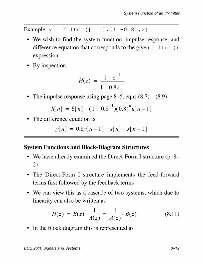
Example: y = filter([1 1],[1 -0.8],x)
• We wish to find the system function, impulse response, anddifference equation that corresponds to the given filter()expression
• By inspection
• The impulse response using page 8–5, eqns (8.7)—(8.9)
• The difference equation is
System Functions and Block-Diagram Structures
• We have already examined the Direct-Form I structure (p. 8–2)
• The Direct-Form I structure implements the feed-forwardterms first followed by the feedback terms
• We can view this as a cascade of two systems, which due tolinearity can also be written as
(8.11)
• In the block diagram this is represented as
H z 1 z1–
+
1 0.8z1–
–------------------------=
h n n 1 0.81–
+ 0.8 nu n 1– +=
y n 0.8y n 1– x n x n 1– + +=
H z B z 1A z ----------- 1
A z ----------- B z = =
ECE 2610 Signals and Systems 8–12

System Function of an IIR Filter
y n x n
z1–
z1–
z1–
z1–
z1–
z1–
w n 1–
w n 2–
w n 3–
b0
b1
b2
b3
a1
a2
a3
w n
Combine commondelay blocks
z1–
z1–
z1–
b0
b1
b2
b3
a1
a2
a3
x n y n
Direct-Form II
w n
A z B z
Shown for N M 3= =
ECE 2610 Signals and Systems 8–13

System Function of an IIR Filter
• The Direct-Form II structure uses fewer delay blocks thanDirect-Form I
The Transposed Structures
• A property of filter block diagrams is that
– When all of the arrows are reversed
– All branch points become summing nodes; all summingnodes become branch points
– The input and output are interchanged
– The system function is unchanged
b1
b2
b3
z1–
z1–
z1–
a1
a2
a3
b0
x n y n
Transposed Direct-Form II
The MATLABfunction filter()implements thisblock diagram
ECE 2610 Signals and Systems 8–14

System Function of an IIR Filter
Relation to the Impulse Response
• From Chapter 7 we know that the impulse response and sys-tem function are related via the z-transform
• For IIR systems more work is required to obtain the z-trans-form
• Consider , where we have learnedthat the impulse response is
• From the definition of the z-transform,
(8.12)
• The sum of (8.12) is an infinite geometric series which ingeneral terms is
• Applying the sum formula to (8.12) results in
(8.13)
– The condition that tells us that the z-transformonly exists for these values of z
– The z-plane region is known as the region of convergence
• We have thus established the following z-transform relation-
y n ay n 1– x n +=
h n anu n =
H z anzn–
n 0=
az1– n
n 0=
= =
S rn
n 0=
11 r–----------- r 1= =
H z az1– n
n 0=
1
1 az1–
–------------------- z a= =
z a
ECE 2610 Signals and Systems 8–15
Poles and Zeros
ship
(8.14)
• We can use this result to find the z-transform of
(8.15)
directly using just linearity and the delay property
• We will learn later that we can work this operation in reverse,and when combined with partial fraction expansion, we willbe able to find the inverse z-transform of almost any rational
Poles and Zeros
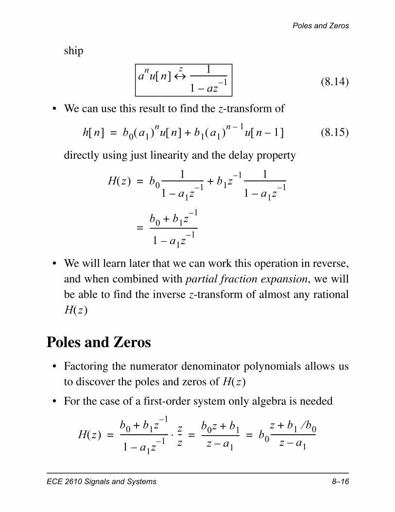
• Factoring the numerator denominator polynomials allows usto discover the poles and zeros of
• For the case of a first-order system only algebra is needed
anu n 1
1 az1–
–-------------------
z
h n b0 a1 nu n b1 a1 n 1–u n 1– +=
H z b01
1 a1z1–
–---------------------- b1z
1– 1
1 a1z1–
–----------------------+=
b0 b1z1–
+
1 a1z1–
–-------------------------=
H z
H z
H z b0 b1z
1–+
1 a1z1–
–------------------------- z
z--
b0z b1+
z a1–-------------------- b0
z b1 b0+
z a1–-----------------------= = =
ECE 2610 Signals and Systems 8–16
Poles and Zeros
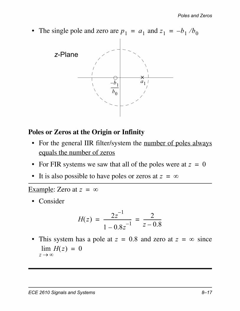
• The single pole and zero are and
Poles or Zeros at the Origin or Infinity
• For the general IIR filter/system the number of poles alwaysequals the number of zeros
• For FIR systems we saw that all of the poles were at
• It is also possible to have poles or zeros at
Example: Zero at
• Consider
• This system has a pole at and zero at since
p1 a1= z1 b1 b0–=
a1b1–
b0---------
z-Plane
z 0=
z =
z =
H z 2z1–
1 0.8z1–
–------------------------ 2
z 0.8–---------------= =
z 0.8= z =H z
z lim 0=
ECE 2610 Signals and Systems 8–17
Poles and Zeros
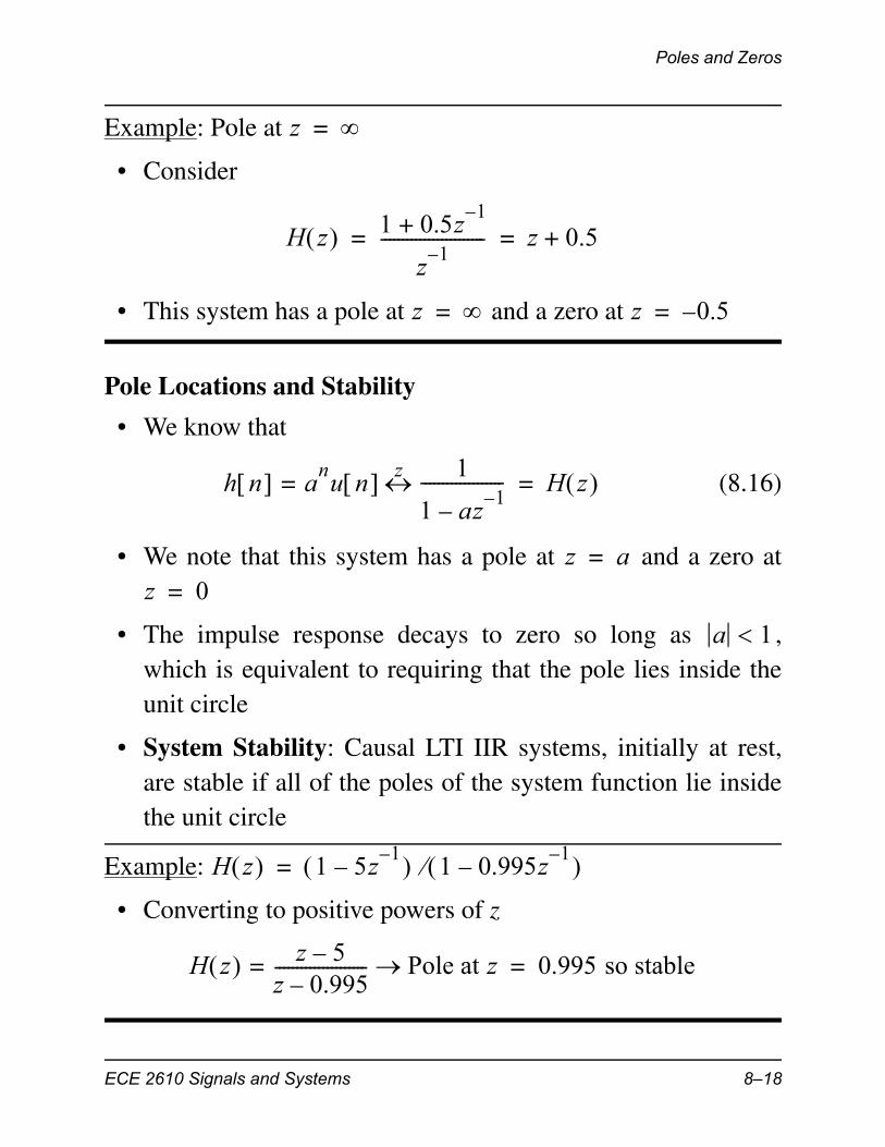
Example: Pole at
• Consider
• This system has a pole at and a zero at
Pole Locations and Stability
• We know that
(8.16)
• We note that this system has a pole at and a zero at
• The impulse response decays to zero so long as ,which is equivalent to requiring that the pole lies inside theunit circle
• System Stability: Causal LTI IIR systems, initially at rest,are stable if all of the poles of the system function lie insidethe unit circle
Example:
• Converting to positive powers of z
z =
H z 1 0.5z1–
+
z1–
------------------------ z 0.5+= =
z = z 0.5–=
h n anu n =
1
1 az1–
–------------------- H z =
z
z a=z 0=
a 1
H z 1 5z1–
– 1 0.995z1–
– =
H z z 5–z 0.995–---------------------= Pole at z 0.995 so stable=
ECE 2610 Signals and Systems 8–18
Poles and Zeros
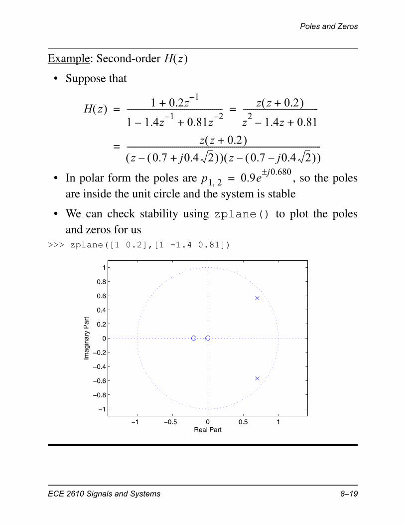
Example: Second-order
• Suppose that
• In polar form the poles are , so the polesare inside the unit circle and the system is stable
• We can check stability using zplane() to plot the polesand zeros for us
>>> zplane([1 0.2],[1 -1.4 0.81])
H z
H z 1 0.2z1–
+
1 1.4z1–
– 0.81z2–
+------------------------------------------------ z z 0.2+
z2
1.4z– 0.81+--------------------------------------= =
z z 0.2+ z 0.7 j0.4 2+ – z 0.7 j0.4 2– –
--------------------------------------------------------------------------------------------------=
p1 2 0.9ej0.680
=
−1 −0.5 0 0.5 1
−1
−0.8
−0.6
−0.4
−0.2
0
0.2
0.4
0.6
0.8
1
Real Part
Imag
inar
y P
art
ECE 2610 Signals and Systems 8–19
Frequency Response of an IIR Filter
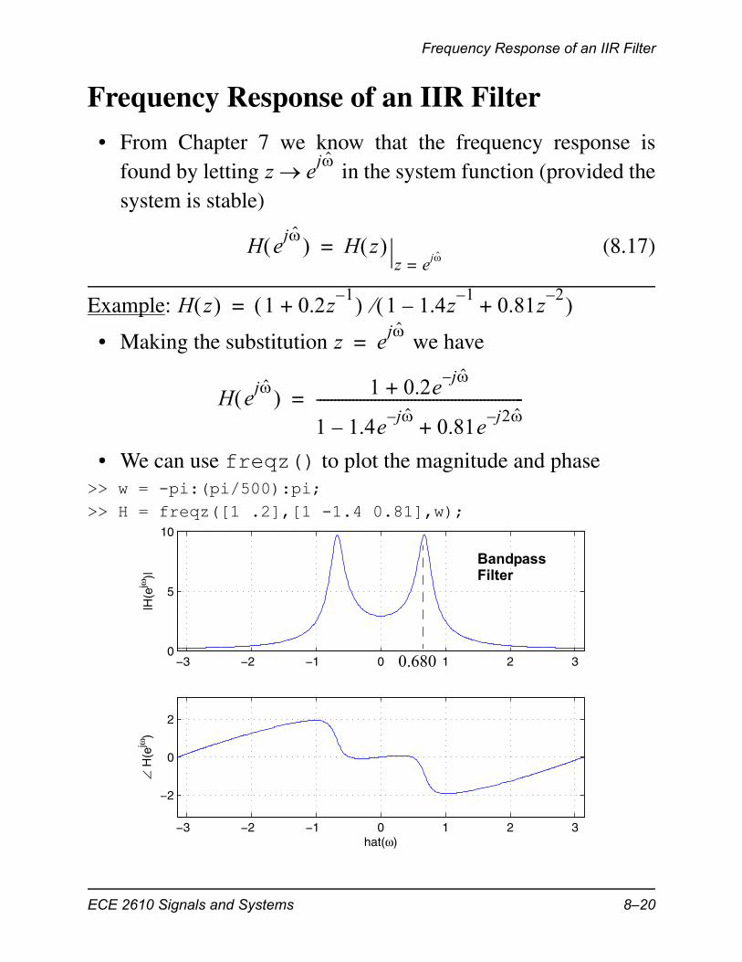
Frequency Response of an IIR Filter
• From Chapter 7 we know that the frequency response isfound by letting in the system function (provided thesystem is stable)
(8.17)
Example:
• Making the substitution we have
• We can use freqz() to plot the magnitude and phase>> w = -pi:(pi/500):pi;>> H = freqz([1 .2],[1 -1.4 0.81],w);
z ej
H ej H z
z ej==
H z 1 0.2z1–
+ 1 1.4z1–
– 0.81z2–
+ =
z ej
=
H ej 1 0.2e
j– +
1 1.4ej–
– 0.81ej– 2
+---------------------------------------------------------=
−3 −2 −1 0 1 2 30
5
10
|H(e
jω)|
−3 −2 −1 0 1 2 3
−2
0
2
∠ H
(ejω
)
hat(ω)
0.680
BandpassFilter
ECE 2610 Signals and Systems 8–20
Frequency Response of an IIR Filter
• This particular filter is a bandpass filter because it has a rela-tive large magnitude response over a narrow band of frequen-cies and small response otherwise
• From the earlier pole-zero analysis, the peak gain is near theangle the poles make to the real axis,
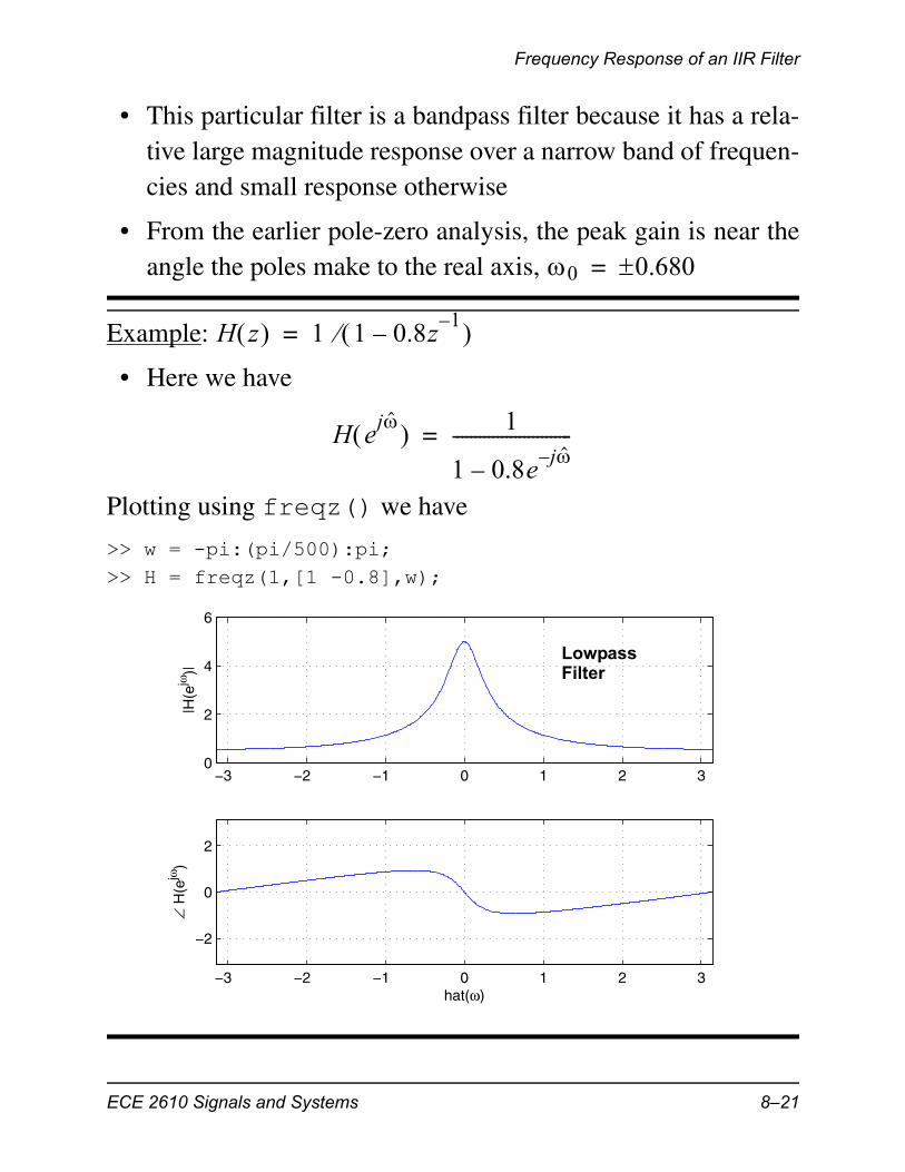
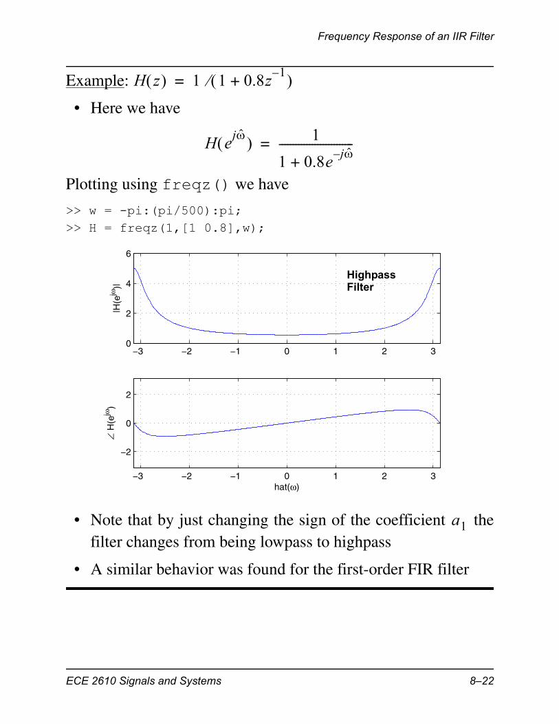
Example:
• Here we have
Plotting using freqz() we have
>> w = -pi:(pi/500):pi;>> H = freqz(1,[1 -0.8],w);
0 0.680=
H z 1 1 0.8z1–
– =
H ej 1
1 0.8ej–
–---------------------------=
−3 −2 −1 0 1 2 30
2
4
6
|H(e
jω)|
−3 −2 −1 0 1 2 3
−2
0
2
∠ H
(ejω
)
hat(ω)
LowpassFilter
ECE 2610 Signals and Systems 8–21
Frequency Response of an IIR Filter
Example:
• Here we have
Plotting using freqz() we have
>> w = -pi:(pi/500):pi;>> H = freqz(1,[1 0.8],w);
• Note that by just changing the sign of the coefficient thefilter changes from being lowpass to highpass
• A similar behavior was found for the first-order FIR filter
H z 1 1 0.8z1–
+ =
H ej 1
1 0.8ej–
+---------------------------=
−3 −2 −1 0 1 2 30
2
4
6
|H(e
jω)|
−3 −2 −1 0 1 2 3
−2
0
2
∠ H
(ejω
)
hat(ω)
HighpassFilter
a1
ECE 2610 Signals and Systems 8–22
The Inverse z-Transform and Applications
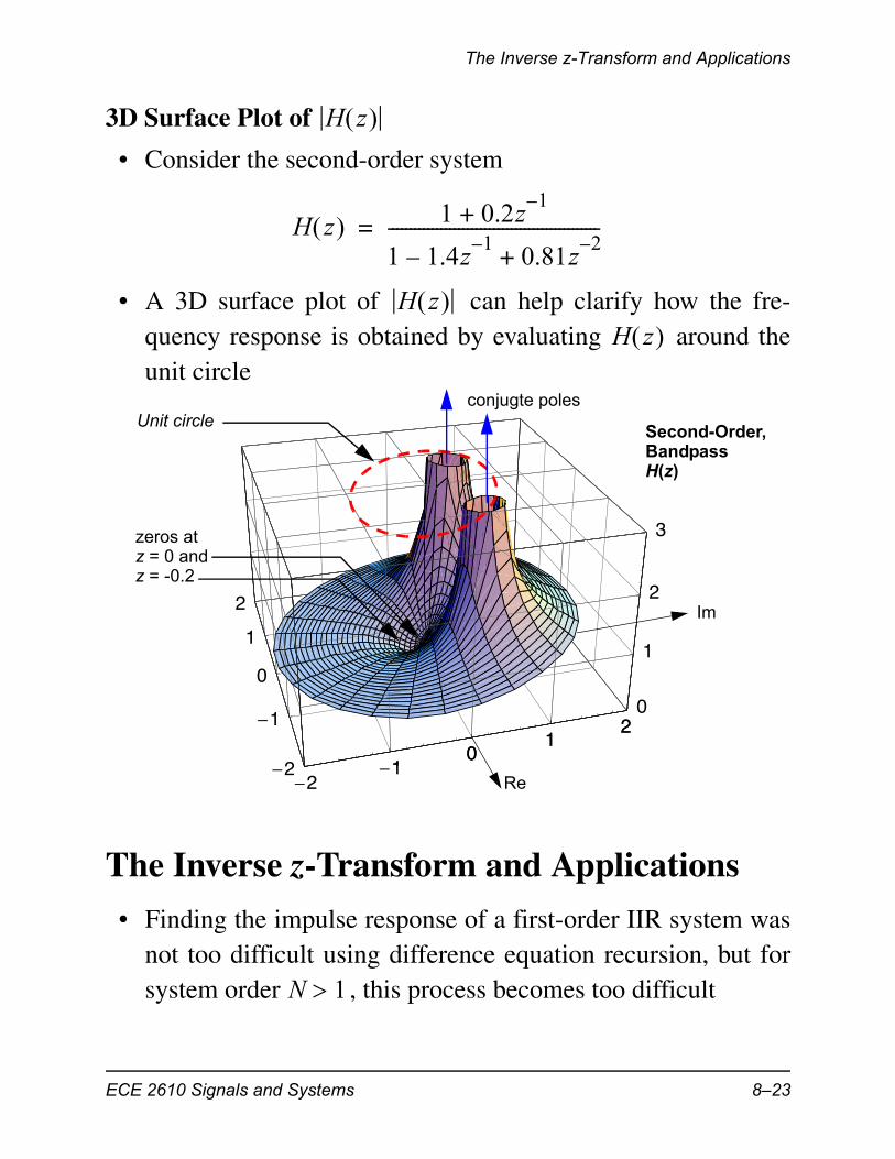
3D Surface Plot of
• Consider the second-order system
• A 3D surface plot of can help clarify how the fre-quency response is obtained by evaluating around theunit circle
The Inverse z-Transform and Applications
• Finding the impulse response of a first-order IIR system wasnot too difficult using difference equation recursion, but forsystem order , this process becomes too difficult
H z
H z 1 0.2z1–
+
1 1.4z1–
– 0.81z2–
+------------------------------------------------=
H z H z
�2�1
01
2
�2
�1
0
1
2
0
1
2
3
10
12
Re
Im
conjugte poles
zeros atz = 0 andz = -0.2
Unit circleSecond-Order,BandpassH(z)
N 1
ECE 2610 Signals and Systems 8–23
The Inverse z-Transform and Applications
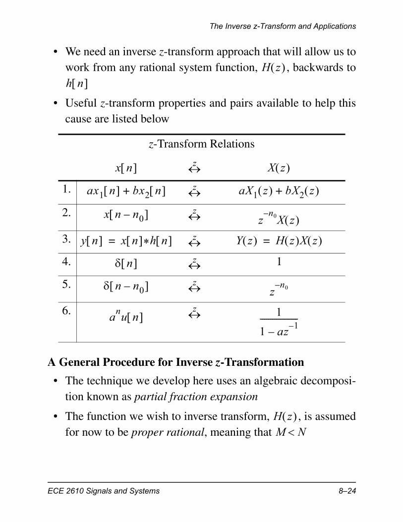
• We need an inverse z-transform approach that will allow us towork from any rational system function, , backwards to
• Useful z-transform properties and pairs available to help thiscause are listed below
A General Procedure for Inverse z-Transformation
• The technique we develop here uses an algebraic decomposi-tion known as partial fraction expansion
• The function we wish to inverse transform, , is assumedfor now to be proper rational, meaning that
z-Transform Relations
1.
2.
3.
4. 1
5.
6.
H z h n
x n z X z
ax1 n bx2 n + z aX1 z bX2 z +
x n n0– z zn0–X z
y n x n *h n = z Y z H z X z =
n z
n n0– z zn0–
anu n z 1
1 az1–
–-------------------
H z M N
ECE 2610 Signals and Systems 8–24
The Inverse z-Transform and Applications
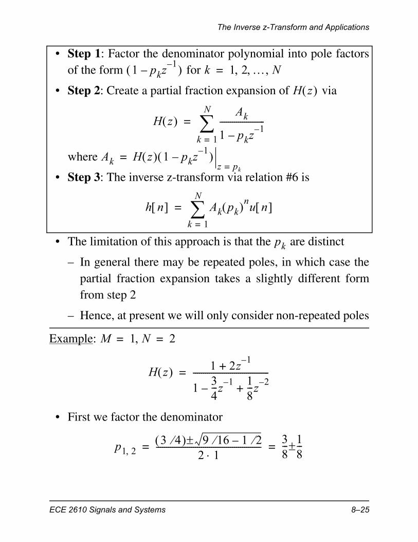
• Step 1: Factor the denominator polynomial into pole factorsof the form for
• Step 2: Create a partial fraction expansion of via
where
• Step 3: The inverse z-transform via relation #6 is
• The limitation of this approach is that the are distinct
– In general there may be repeated poles, in which case thepartial fraction expansion takes a slightly different formfrom step 2
– Hence, at present we will only consider non-repeated poles
Example:
• First we factor the denominator
1 pkz1–
– k 1 2 N =
H z
H z Ak
1 pkz1–
–----------------------
k 1=
N
=
Ak H z 1 pkz1–
– z pk=
=
h n Ak pk nu n k 1=
N
=
pk
M 1 N 2= =
H z 1 2z1–
+
134---z
1––
18---z
2–+
-------------------------------------=
p1 23 4 9 16 1 2–
2 1---------------------------------------------------
38--- 1
8---= =
ECE 2610 Signals and Systems 8–25
The Inverse z-Transform and Applications
• Solving for
• Solving for
• So,
• Inverse z-transform term-by-term using #6
H z 1 2z1–
+
112---z
1––
114---z
1––
---------------------------------------------------
A1
112---z
1––
--------------------A2
114---z
1––
--------------------+= =
A1
A11 2z
1–+
112---z
1––
114---z
1––
--------------------------------------------------- 1
12---z
1––
z 1 2=
=
1 2z1–
+
114---z
1––
--------------------
z 1– 2=
1 4+
1 12---–
------------ 10= ==
A2
A21 2z
1–+
112---z
1––
114---z
1––
--------------------------------------------------- 1
14---z
1––
z 1 4=
=
1 2z1–
+
112---z
1––
--------------------
z 1– 4=
1 8+1 2–------------ 9–= ==
H z 10
112---z
1––
-------------------- 9
114---z
1––
--------------------–=
ECE 2610 Signals and Systems 8–26

The Inverse z-Transform and Applications
• The MATLAB signal processing toolbox has a function thatcan perform partial fraction expansion
>> help residuez RESIDUEZ Z-transform partial-fraction expansion. [R,P,K] = RESIDUEZ(B,A) finds the residues, poles and direct terms of the partial-fraction expansion of B(z)/A(z), B(z) r(1) r(n) ---- = ------------ +... ------------ + k(1) + k(2)z^(-1) ... A(z) 1-p(1)z^(-1) 1-p(n)z^(-1) B and A are the numerator and denominator polynomial coefficients, respectively, in ascending powers of z^(-1). R and P are column vectors containing the residues and poles, respectively. K contains the direct terms in a row vector. The number of poles is n = length(A)-1 = length(R) = length(P) The direct term coefficient vector is empty if length(B) < length(A); otherwise, length(K) = length(B)-length(A)+1 If P(j) = ... = P(j+m-1) is a pole of multiplicity m, then the expansion includes terms of the form R(j) R(j+1) R(j+m-1) -------------- + ------------------ + ... + ------------------ 1 - P(j)z^(-1) (1 - P(j)z^(-1))^2 (1 - P(j)z^(-1))^m [B,A] = RESIDUEZ(R,P,K) converts the partial-fraction expansion back to B/A form.
• Using residuez() we find:>> [A,p,K] = residuez([1 2],[1 -3/4 1/8])
A = 10 % The partial fraction coefficients -9 % agreep = 5.0000e-01 % The pole factoring agrees 2.5000e-01 % K = [] % Results from long division % to make proper rational (NA here).
h n 1012--- nu n 9
14--- nu n –=
ECE 2610 Signals and Systems 8–27
The Inverse z-Transform and Applications
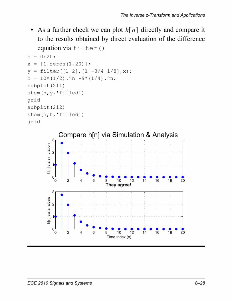
• As a further check we can plot directly and compare itto the results obtained by direct evaluation of the differenceequation via filter()
n = 0:20;x = [1 zeros(1,20)];y = filter([1 2],[1 -3/4 1/8],x);h = 10*(1/2).^n -9*(1/4).^n;subplot(211)stem(n,y,'filled')gridsubplot(212)stem(n,h,'filled')grid
h n
0 2 4 6 8 10 12 14 16 18 200
1
2
3
h[n]
via
sim
ulat
ion
0 2 4 6 8 10 12 14 16 18 200
1
2
3
h[n]
via
ana
lysi
s
Time Index (n)
Compare h[n] via Simulation & Analysis
They agree!
ECE 2610 Signals and Systems 8–28
The Inverse z-Transform and Applications
Example:
• Find for an IIR system having input andsystem function
• We will first find
• From table entry #6 with
• As a result of table entry #3
• We now use a partial fraction expansion over the three realpoles 1, -1/3, and 1/2
• Solving for the coefficients
y n x n *h n =
y n x n 2u n =
H z 1 z1–
+
116---z
1––
16---z
2––
-------------------------------------=
Y z
a 1=
X z 2
1 z1–
–----------------=
Y z X z H z 2 2z1–
+
1 z1–
– 116---z
1––
16---z
2––
----------------------------------------------------------------= =
2 2z1–
+
1 z1–
– 113---z
1–+
112---z
1––
-------------------------------------------------------------------------=
Y z A1
1 z1–
–----------------
A2
113---z
1–+
--------------------A3
112---z
1––
--------------------+ +=
ECE 2610 Signals and Systems 8–29
The Inverse z-Transform and Applications
• Finally,
and using #6 to inverse transform term-by-term
We can check this result using residuez()>> [A,p,K] = residuez([2 2],conv([1 -1],[1 -1/6 -1/6]))
A = 6.0000e+00 <== agrees with A1 = 6 -3.6000e+00 <== agrees with A3 = -18/5 -4.0000e-01 <== agrees with A2 = -2/5
A12 2z
1–+
113---z
1–+
112---z
1––
---------------------------------------------------
z 1– 1=
2 2+43--- 1
2---
------------ 6= = =
A22 2z
1–+
1 z1–
– 112---z
1––
-----------------------------------------------
z 1– 3–=
2 6–
452---
------------ 25---–= = =
A32 2z
1–+
1 z1–
– 113---z
1–+
-----------------------------------------------
z 1– 2=
2 4+
1–53---
------------- 185------–= = =
Y z 6
1 z1–
–---------------- 2 5
113---z
1–+
--------------------– 18 5
112---z
1––
--------------------–=
y n 6u n 25--- 1
3---–
nu n –185------ 1
2--- nu n –=
ECE 2610 Signals and Systems 8–30

The Inverse z-Transform and Applications
p = 1.0000e+00 5.0000e-01 -3.3333e-01
K = []
• The results agree!
• The partial fraction expansion technique requires that
• If the rational function does not satisfy this condition we canperform long division to reduce the order of the denominatorto the point where
Example: Long Division
• Consider
where (not proper rational)
• Perform long division
• We now have reduced to the form
M N
M N
Y z 2 2.4z1–
– 0.4z2–
–
1 0.3z1–
– 0.4z2–
–---------------------------------------------=
N M 2= =
1 0.3z1–
– 0.4z2–
– 2 2.4z1–
– 0.4z2–
–
1
1 0.3z1–
– 0.4z2–
–
1 2.1z1–
–
Y z
Y z 1 1 2.1z1–
–
1 0.3z1–
– 0.4z2–
–---------------------------------------------+=
ECE 2610 Signals and Systems 8–31

The Inverse z-Transform and Applications
• We can now perform a partial fraction expansion on the ratio-nal function
• The coefficients are
• Finally,
and
• We can again check this with residuez(); which willautomatically perform long division
>> [A,p,K] = residuez([2 -2.4 -0.4],[1 -0.3 -0.4])
A = -1 <== agrees with A2 = -1 2 <== agrees with A1 = 2
Y z 1 2.1z1–
–
1 0.3z1–
– 0.4z2–
–--------------------------------------------- 1 2.1z
1––
1 0.5z1–
+ 1 0.8z1–
– -----------------------------------------------------------= =
A1
1 0.5z1–
+------------------------
A2
1 0.8z1–
–------------------------+=
A11 2.1z
1––
1 0.8z1–
–------------------------
z 1– 2–=
1 4.2+1 1.6+---------------- 2= = =
A21 2.1z
1––
1 0.5z1–
+------------------------
z 1– 1.25=
1 2.625–1 0.625+---------------------- 1–= = =
Y z 1 2
1 0.5z1–
+------------------------ 1
1 0.8z1–
–------------------------–+=
y n n 2 0.5– nu n 0.8 nu n –+=
ECE 2610 Signals and Systems 8–32

Steady-State Response and Stability
p = 8.0000e-01 -5.0000e-01
K = 1 <== Long division term
• The value is the result of long division (see the helpfor residuez())
• The answers agree!
Steady-State Response and Stability
• The sinusoidal steady-state response developed in Chapter 6for FIR filters also holds for IIR filters
• It can be shown (see Text Section 8-8 for more details, espe-cially for ) that for
(8.18)
and an IIR system with , the system output willbe
(8.19)
where are the poles of and the arethe corresponding partial fraction coefficients
• The first term represents the transient response, which pro-vided all the poles of lie inside the unit circle, willdecay to zero, leaving just the sinusoidal term
K 1=
N 1=
x n ej0nu n =
H z N M
y n Ak pk nu n k 1=
N
H ej0 ej0nu n +=
pk k 1 N = H z Ak
H z
ECE 2610 Signals and Systems 8–33

Steady-State Response and Stability
• For the output to reach sinusoidal steady-state we must have to insure that the transient term (first term) decays to
zero, this then insures that the system is stable
• Summary: Poles inside the unit circle to insure stability
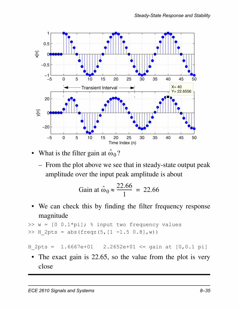
Example:
• Input a cosine with starting at to the sys-tem
• This is a second-order IIR filter, so the transient term consistsof two exponentials
• Second-order system will be studied in more detail in thenext section
• Observe the transient using MATLAB
>> n = -5:50;>> x = cos(2*pi/20*n).*ustep(n,0);>> y = filter(5,[1 -1.5 0.8],x);>> subplot(211)>> stem(n,x,'filled')>> axis([-5 50 -1 1]); grid>> ylabel('x[n]')>> subplot(212)>> stem(n,y,'filled')>> axis([-5 50 -30 30]); grid>> ylabel('y[n]')>> xlabel('Time Index (n)')
pk 1
x n 2 20 n u n cos=
0 0.1= n 0=
H z 5
1 1.8z1–
– 0.9z2–
+---------------------------------------------=
ECE 2610 Signals and Systems 8–34
Steady-State Response and Stability
• What is the filter gain at ?
– From the plot above we see that in steady-state output peakamplitude over the input peak amplitude is about
• We can check this by finding the filter frequency responsemagnitude
>> w = [0 0.1*pi]; % input two frequency values>> H_2pts = abs(freqz(5,[1 -1.5 0.8],w))
H_2pts = 1.6667e+01 2.2652e+01 <= gain at [0,0.1 pi]
• The exact gain is 22.65, so the value from the plot is veryclose
−5 0 5 10 15 20 25 30 35 40 45 50−1
−0.5
0
0.5
1x[
n]
−5 0 5 10 15 20 25 30 35 40 45 50
−20
0
20
X= 40Y= 22.6556
y[n]
Time Index (n)
Transient Interval
0
Gain at 022.66
1------------- 22.66=
ECE 2610 Signals and Systems 8–35
Second-Order Filters
Second-Order Filters
• Second-order IIR filters allow for the possibility of complexconjugate pole and zero pairs, yet still have real coefficients
• The general second-order system function is
(8.20)
• The corresponding difference equation is
(8.21)
• The direct-form I and direct-form II structures, discussed onpages 8–2 and 8–13 respectively, can be used to implement(8.21)
Poles and Zeros
• To identify the poles and zeros of we can first convertto positive powers of z and then factor into poles and zeros
• The coefficients are related to the roots (poles & zeros) via
(8.22)
H z b0 b1z
1–b2z
2–+ +
1 a1z1–
– a2z2–
–---------------------------------------------=
y n a1y n 1– a2y n 2– +=
b0x n b1x n 1– b2x n 2– + + +
H z
H z b0z
2b1z b2+ +
z2a1z– a2+
------------------------------------- b0
z z1– z z2– z p1– z p2–
-------------------------------------= =
b1 b0 z1 z2+ –= b2 b0 z1z2=
a1 p1 p2+= a2 p1p2–=
ECE 2610 Signals and Systems 8–36
Second-Order Filters
• Given real coefficients, numerator and denominator, the rootsoccur either as two real values or as a complex-conjugate pair
• Poles: From the quadratic formula
– Real poles occur when
– Complex-conjugate poles occur otherwise, and are givenby
where
• Zeros: Similar results hold for the zeros if we factor out and then replace with and replace with
p1 2a1 a1
24a2+
2----------------------------------=
a12
4a2+ 0
p1 212---a1 j
12--- a1
2– 4a2–=
rej
=
r a2–=
cos1– a1
2 a2–----------------
=
b0a1 b1 b0– a2
b2 b0–
ECE 2610 Signals and Systems 8–37
Second-Order Filters
Example: Complex Poles and Zeros
• Consider
• Apply the quadratic formula to the numerator and denomina-tor to find the zeros and poles
• We can use the MATLAB function tf2zp() to convert thesystem function form to a zero pole form, plus a gain term
>> [z,p,K] = tf2zp([3 2 2.5],[1 -1.5 0.8])
z = -3.3333e-01 + 8.4984e-01i % these agree with the -3.3333e-01 - 8.4984e-01i % hand calculationsp = 7.5000e-01 + 4.8734e-01i 7.5000e-01 - 4.8734e-01iK = 3 % K is the same as b0 in this case
H z 3 2z1–
2.5z2–
+ +
1 1.5z1–
– 0.8z2–
+---------------------------------------------
3 123---z
1– 2.53
-------z2–
+ +
1 1.5z1–
– 0.8z2–
+---------------------------------------------------= =
z1 22 2
24 3 2.5 ––
2 3-----------------------------------------------------=
0.3333 j0.8498– 0.9129ej1.9446
==
p1 21.5 1.5
24 1 0.8 –
2 1-----------------------------------------------------------=
0.7500 j0.4873 0.8944ej0.5762
==
ECE 2610 Signals and Systems 8–38
Second-Order Filters
Impulse Response
• Using a partial fraction expansion we can inverse transformany rational back to the impulse response
• Given
(8.23)
we first perform long division to reduce the numerator orderby one
• It can be shown that the partial fraction expansion will be ofthe form
(8.24)
where
• The impulse response is found using the table on page 8–24
(8.25)
• This is a very general result, because the poles may be eitherreal or complex conjugates
– Note that if (no long division is required) then thedelta function term in (8.25) is not needed
H z h n
H z b0 b1z
1–b2z
2–+ +
1 a1z1–
– a2z2–
–---------------------------------------------
b0 b1z1–b2z
2–+ +
1 p1z1–
– 1 p2z1–
– ------------------------------------------------------= =
H z b2
a2-----–
A1
1 p1z1–
–----------------------
A2
1 p2z1–
–----------------------+ +=
Ak H z 1 pkz1–
– z pk=
=
h n b2
a2----- n – A1 p1 nu n A2 p2 nu n + +=
b2 0=
ECE 2610 Signals and Systems 8–39
Second-Order Filters
– For complex conjugates poles further simplification is pos-sible because and will also be complex conjugates
• Complex Conjugate Poles: To simplify (8.25) for this casewe first write and in polar form
(8.26)
– We can now write
(8.27)
and (8.25) specializes to
(8.28)
– We also see from this form that if we place the poles on theunit circle, the impulse response will contain a pure sinu-soid, since
Example: Conjugate Poles Inside the Unit Circle
• Find the impulse response corresponding to
• The partial fraction expansion is of the form
A1 A2
A1 p1
A1 ej=
p1 rej
=
A1 p1 n A2 p2 n+ rnej n + rne j n + –+=
2rn n + cos=
b2
a2----- n – 2rn n + u n cos+
rn
1n 1=
H z 3 z1–
+
134---ej 4
z1–
– 1
34---e
j– 4z
1––
-------------------------------------------------------------------------------=
ECE 2610 Signals and Systems 8–40

Second-Order Filters
• We know that
• Using the general result of (8.28) we see that ,, , and , so
• Check using residuez()>> [A,p,K] = residuez([3 1],[1 -2*3/4*cos(pi/4) 9/16])
A = 1.5000e+00 - 2.4428e+00i 1.5000e+00 + 2.4428e+00i
p = 5.3033e-01 + 5.3033e-01i 5.3033e-01 - 5.3033e-01i
K = []
>> [abs(A(1)) angle(A(1))] % Get mag and angle of A1
ans = 2.8666e+00 -1.0201e+00 % The results agree
H z A1
134---ej 4
z1–
–--------------------------------
A2
134---e
j– 4z
1––
-----------------------------------+=
A2 A1*=
A13 z
1–+
134---e
j 4–z
1––
-----------------------------------
z 1– 43---e j 4–=
343---e
j 3–+
1 j+---------------------------= =
2.867ej1.020–
=
2.867= 1.020–= r 0.75= 4=
h n 2 2.867 0.75 n 4---n 1.020– cos =
ECE 2610 Signals and Systems 8–41
Second-Order Filters
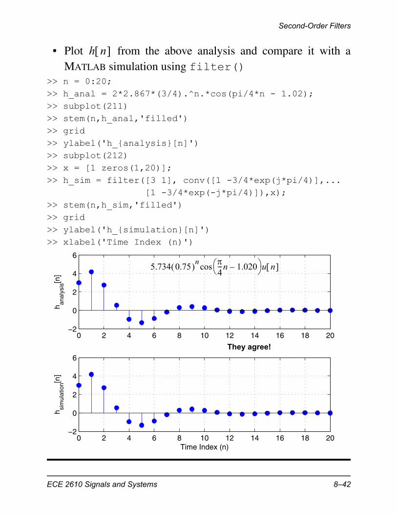
• Plot from the above analysis and compare it with aMATLAB simulation using filter()
>> n = 0:20;>> h_anal = 2*2.867*(3/4).^n.*cos(pi/4*n - 1.02);>> subplot(211)>> stem(n,h_anal,'filled')>> grid>> ylabel('h_{analysis}[n]')>> subplot(212)>> x = [1 zeros(1,20)];>> h_sim = filter([3 1], conv([1 -3/4*exp(j*pi/4)],... [1 -3/4*exp(-j*pi/4)]),x);>> stem(n,h_sim,'filled')>> grid>> ylabel('h_{simulation}[n]')>> xlabel('Time Index (n)')
h n
0 2 4 6 8 10 12 14 16 18 20−2
0
2
4
6
h anal
ysis
[n]
0 2 4 6 8 10 12 14 16 18 20−2
0
2
4
6
h sim
ulat
ion[n
]
Time Index (n)
They agree!
5.734 0.75 n 4---n 1.020– u n cos
ECE 2610 Signals and Systems 8–42
Second-Order Filters
Frequency Response
(8.29)
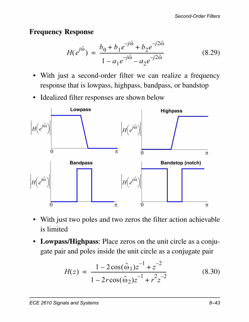
• With just a second-order filter we can realize a frequencyresponse that is lowpass, highpass, bandpass, or bandstop
• Idealized filter responses are shown below
• With just two poles and two zeros the filter action achievableis limited
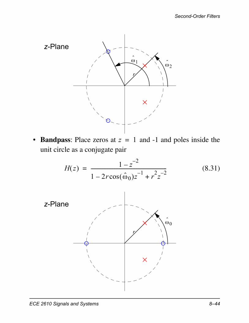
• Lowpass/Highpass: Place zeros on the unit circle as a conju-gate pair and poles inside the unit circle as a conjugate pair
(8.30)
H ej
b0 b1ej–
b2ej2–
+ +
1 a1ej–
a2ej2–
––-----------------------------------------------------=
0
H ej
Lowpass
0
H ej
Highpass
0
H ej
Bandpass
0
H ej
Bandstop (notch)
H z 1 2 1 z 1–
cos– z2–
+
1 2r 2 z 1–cos– r
2z
2–+
--------------------------------------------------------------=
ECE 2610 Signals and Systems 8–43
Second-Order Filters
• Bandpass: Place zeros at and -1 and poles inside theunit circle as a conjugate pair
(8.31)
z-Plane
1 2
r
z 1=
H z 1 z2–
–
1 2r 0 z 1–cos– r
2z
2–+
--------------------------------------------------------------=
z-Plane
0
r
ECE 2610 Signals and Systems 8–44
Example of an IIR Lowpass Filter
• Bandstop (notch):
(8.32)
– See the final project
Example of an IIR Lowpass Filter
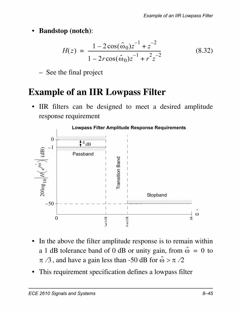
• IIR filters can be designed to meet a desired amplituderesponse requirement
• In the above the filter amplitude response is to remain withina 1 dB tolerance band of 0 dB or unity gain, from to
, and have a gain less than -50 dB for
• This requirement specification defines a lowpass filter
H z 1 2 0 z 1–
cos– z2–
+
1 2r 0 z 1–cos– r
2z
2–+
--------------------------------------------------------------=20
log 10
Hej
(dB
)
0
3---
2---
0
50–
dB
Passband
Stopband
Tra
nsiti
on B
and
1–
Lowpass Filter Amplitude Response Requirements
0= 3 2
ECE 2610 Signals and Systems 8–45

Example of an IIR Lowpass Filter
• A variety of IIR filters can be designed to meet these require-ments, one such filter type is an elliptic filter, which is avail-able in the MATLAB signal processing toolbox
>> ellipord(2*(pi/3/(2*pi)),2*(pi/2/(2*pi)),1,50)
ans = 5 % The required filter order, N, to meet % the design requirements.>> [b,a] = ellip(5,1,50,2*(pi/3/(2*pi)));%design filter>> b = 1.9431e-02 2.1113e-02 3.7708e-02 3.7708e-02 2.1113e-02 1.9431e-02 % M=5>> a 1.0000e+00 -2.7580e+00 4.0110e+00 -3.3711e+00 1.6542e+00 -3.7959e-01 % N=5>> zplane(b,a)>> w = -pi:(pi/500):pi;>> H = freqz(b,a,w);>> subplot(211); plot(w,20*log10(abs(H)))>> subplot(212); plot(w,angle(H))
−1 −0.5 0 0.5 1
−1
−0.8
−0.6
−0.4
−0.2
0
0.2
0.4
0.6
0.8
1
Real Part
Imag
inar
y P
art
ECE 2610 Signals and Systems 8–46
Example of an IIR Lowpass Filter
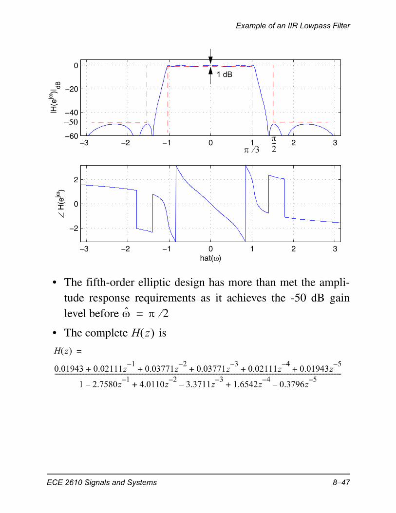
• The fifth-order elliptic design has more than met the ampli-tude response requirements as it achieves the -50 dB gainlevel before
• The complete is
−3 −2 −1 0 1 2 3−60
−40
−20
0
|H(e
jω)|
dB
−3 −2 −1 0 1 2 3
−2
0
2
∠ H
(ejω
)
hat(ω)
32---
50–
1 dB
2=
H z H z =
0.01943 0.02111z1–
0.03771z2–
0.03771z3–
0.02111z4–
0.01943z5–
+ + + + +
1 2.7580z1–
– 4.0110z2–
3.3711z3–
– 1.6542z4–
0.3796z5–
–+ +----------------------------------------------------------------------------------------------------------------------------------------------------------------------------------------------
ECE 2610 Signals and Systems 8–47

Example of an IIR Lowpass Filter
ECE 2610 Signals and Systems 8–48
Related Documents


![-10 0 · Design IIR Bandpass Filters In this post, I present a method to design Butterworth IIR bandpass filters. My previous post [1] covered lowpass IIR filter design, and provided](https://static.cupdf.com/doc/110x72/5ebb71a95c880514701dd82d/10-0-design-iir-bandpass-filters-in-this-post-i-present-a-method-to-design-butterworth.jpg)