IEOR 180 Senior Project Toni Geralde Mona Gohil Nicolas Gomez Lily Surya Patrick Tam Optimizing Electricity Procurement for the City of Palo Alto.

IEOR 180 Senior Project

Toni GeraldeMona Gohil

Nicolas GomezLily Surya

Patrick Tam

Optimizing Electricity

Procurement for the

City of Palo Alto

Outline

• City of Palo Alto• Energy deregulation• Tradeoffs• Palo Alto’s current decision making

tools• Our linear optimization model• Results

Founded: 1900Area: 26 square milesCustomers: 58,100 including• residential homes• small businesses• corporate offices• manufacturing facilities• excluding Stanford University Campus

Company Background

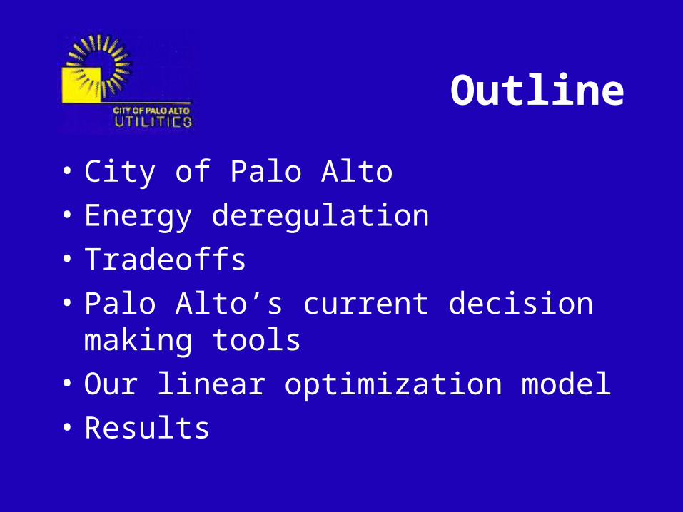
California Energy

Deregulation• Began January 1, 1998• Open buyer and seller

market for electricity– Purchase Energy $X per

Mega Watt Hour

California Energy Market

Inflexible products:

constant amount/ fixed prices

Forwards

High Load

Load Load

All Week

Flexible products:

variable amounts

Spot market

WAPA

Trade-Offs

• Futures contracts: – safeguard against price spikes versus

cost of premium

• Spot Market– flexibility of amount versus exposure to

risk

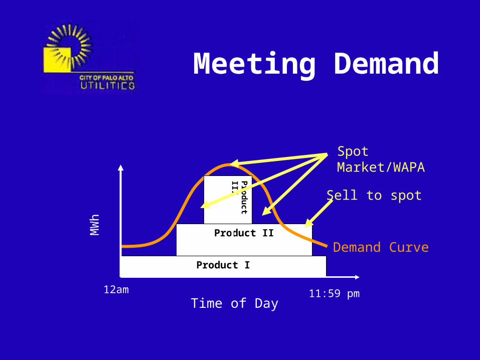
Meeting Demand

Time of Day

MW

h

Product II

Spot Market/WAPA

Demand CurveProduct I

Sell to spot

12am 11:59 pm

priP

rod

uc

t III

Palo Alto Model:Challenges

• How much WAPA should be utilized– capacity charge based on maximum amount

• How much to purchase in advance via forwards

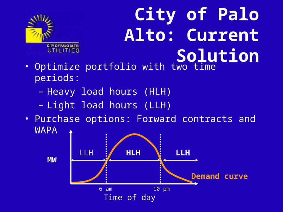
• Optimize portfolio with two time periods:– Heavy load hours (HLH)– Light load hours (LLH)

• Purchase options: Forward contracts and WAPA

City of Palo Alto: Current Solution

LLH HLH LLH

Demand curve

MW

Time of day6 am 10 pm

Problem Statement

• Optimize available energy sources with additional energy products and additional time periods to accommodate them: – WAPA – HLH forwards– LLH forwards– E3 blocks– All week forwards

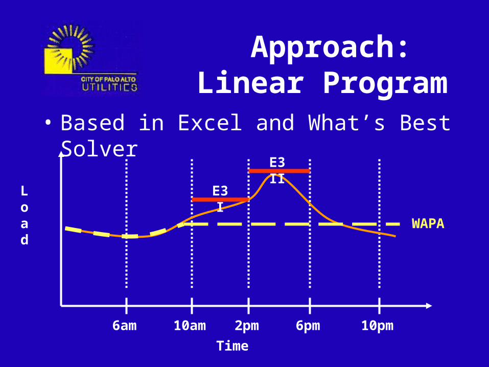
Approach: Linear Program

• Based in Excel and What’s Best Solver

WAPA

E3 I

E3 II

Time

Load

6am 10am 2pm 6pm 10pm

Available Data

• Forecasted Load– Hourly demand for one year

• Forecasted Market Prices• Fixed Contract prices

Model features

• Flexible: Let the user input values for all parameters.

• Accurate: It follows the power demand closely by dividing the month into 150 periods.

• Handle risk: Control exposure to spot market for different demand loads.

• Automated

Subscripts

b=Block index (1,…,5) d=Day index (1,…,31)K=Week index (1,…,5)

Decision variables

• Power from WAPAbd

• MAX

• Power from High Load Forward

• Power from Low Load Forward

• Power from All Week Forward

• Power from E3bk

Parameters

• Upper and Lower limit for WAPA

• WAPA capacity cost

• Variable Cost of each product

• Demand Loadbd, during each period

Objective function

MIN Cost of Product bdk * Product bdk

+ (WAPA Capacity Cost * MAX)

- (Load bdk - Product bdk)*Cost Forward bdk

Constraints

• WAPA Upper and Lower limit constraints

• MAX >= WAPAbd.

• Satisfy all demand

• All variables >= 0.

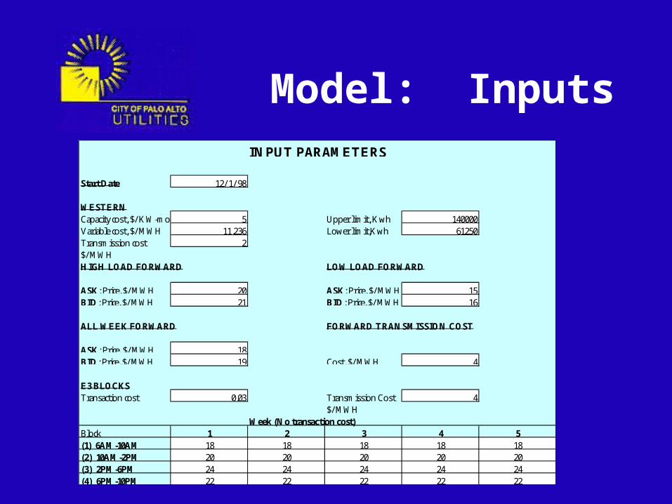
Model: Inputs

Start Date 12/ 1/ 98

WESTERNCapacity cost, $/ KW-mo 5 Upper limit, Kwh 140000Variable cost, $/ MWH 11.236 Lower limit,Kwh 61250Transmission cost 2$/ MWH HIGH LOAD FORWARD LOW LOAD FORWARD

ASK: Price, $/ MWH 20 ASK: Price, $/ MWH 15BID: Price, $/ MWH 21 BID: Price, $/ MWH 16

ALL WEEK FORWARD FORWARD TRANSMISSION COST

ASK: Price, $/ MWH 18BID: Price, $/ MWH 19 Cost, $/ MWH 4

E3 BLOCKSTransaction cost 0.03 Transmission Cost 4

$/ MWHWeek (No transaction cost)

Block 1 2 3 4 5(1) 6AM-10AM 18 18 18 18 18(2) 10AM-2PM 20 20 20 20 20(3) 2PM-6PM 24 24 24 24 24(4) 6PM-10PM 22 22 22 22 22

INPUT PARAMETERS

Quantifying Risk

• Risk Defined:– exposure to spot market

• Risk Implementation– % exposure to spot market

• during high load periods• during normal load periods

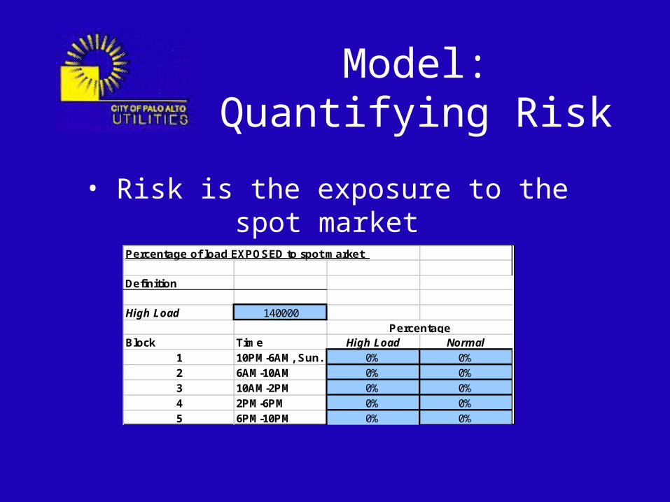
Percentage of load EXPOSED to spot market

Definition

High Load 140000

Block Time High Load Normal1 10PM-6AM, Sun. 0% 0%2 6AM-10AM 0% 0%3 10AM-2PM 0% 0%4 2PM-6PM 0% 0%5 6PM-10PM 0% 0%

Percentage

Model: Quantifying Risk

• Risk is the exposure to the spot market

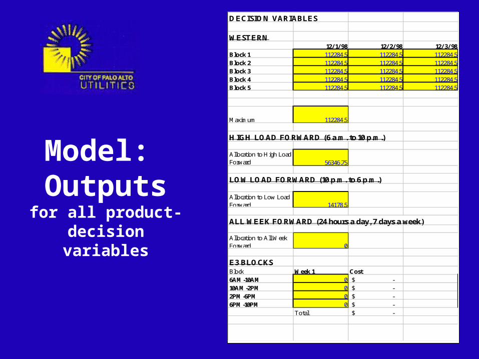
Model: Outputsfor all product-

decision variables

DECISION VARIABLES

WESTERN12/1/98 12/2/98 12/3/98

Block 1 112284.5 112284.5 112284.5Block 2 112284.5 112284.5 112284.5Block 3 112284.5 112284.5 112284.5Block 4 112284.5 112284.5 112284.5Block 5 112284.5 112284.5 112284.5

Maximum 112284.5

HIGH LOAD FORWARD (6 a.m. to 10 p.m.)

Allocation to High Load Forward 56346.75

LOW LOAD FORWARD (10 p.m. to 6 p.m.)

Allocation to Low Load Forward 14178.5

ALL WEEK FORWARD (24 hours a day, 7 days a week)

Allocation to All Week Forward 0

E3 BLOCKSBlock Week 1 Cost6AM-10AM 0 -$ 10AM-2PM 0 -$ 2PM-6PM 0 -$ 6PM-10PM 0 -$

Total -$

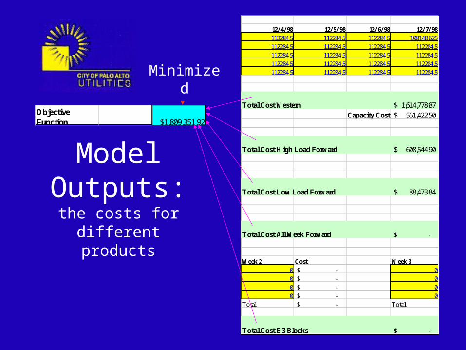
12/4/98 12/5/98 12/6/98 12/7/98112284.5 112284.5 112284.5 108148.625112284.5 112284.5 112284.5 112284.5112284.5 112284.5 112284.5 112284.5112284.5 112284.5 112284.5 112284.5112284.5 112284.5 112284.5 112284.5

Total Cost Western 1,614,778.87$ Capacity Cost 561,422.50$

Total Cost High Load Forward 608,544.90$

Total Cost Low Load Forward 88,473.84$

Total Cost All Week Forward -$

Week 2 Cost Week 30 -$ 00 -$ 00 -$ 00 -$ 0

Total -$ Total

Total Cost E3 Blocks -$

Model Outputs:

the costs for different products

Objective Function $1,809,351.92

Minimized

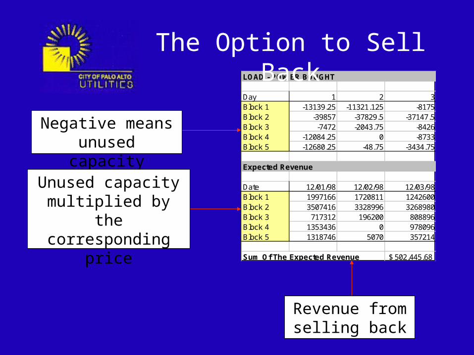
LOAD - POWER BOUGHT

Day 1 2 3Block 1 -13139.25 -11321.125 -8175Block 2 -39857 -37829.5 -37147.5Block 3 -7472 -2043.75 -8426Block 4 -12084.25 0 -8733Block 5 -12680.25 -48.75 -3434.75

Expected Revenue

Date 12/01/98 12/02/98 12/03/98Block 1 1997166 1720811 1242600Block 2 3507416 3328996 3268980Block 3 717312 196200 808896Block 4 1353436 0 978096Block 5 1318746 5070 357214

Sum Of The Expected Revenue 502,445.68$

The Option to Sell Back

Negative means unused capacity

Unused capacity multiplied by the

corresponding price

Revenue from selling back

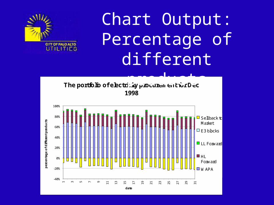
The portfolio of electricity procurement for Dec 1998

-40%

-20%

0%

20%

40%

60%

80%

100%

1 3 5 7 9 11 13 15 17 19 21 23 25 27 29 31

date

per

cen

tag

e o

f d

iffe

ren

t p

rod

uct

s

Sell back toMarket

E3 blocks

LL Forward

HLForward

WAPA

Chart Output: Percentage of

different products

Quantifying Results

Model Comparison• Run models under various scenarios

– Heavy load– Light load – Normal load

• Calculate cost reduction under new model

Model Comparison

• Based on same inputs– prices– forecasted demand

• Compare models against an actual load– Actual load = average load during

time intervals utilized in UCB model

Model Comparison

• UCB Model is inherently better than Palo Alto’s current Model.

Time

Load

6am 10am 2pm 6pm 10pm

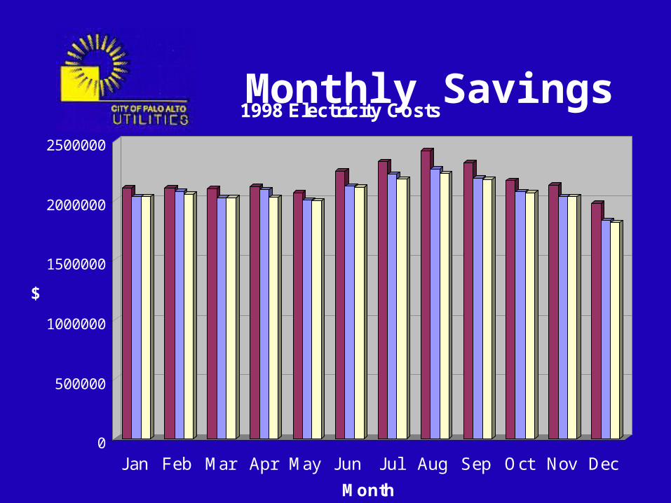
Monthly Savings

0

500000

1000000

1500000

2000000

2500000

$

Jan Feb Mar Apr May Jun Jul Aug Sep Oct Nov Dec

Month

1998 Electricity Costs

Annual Savings

$24,000,000.00

$24,200,000.00

$24,400,000.00

$24,600,000.00

$24,800,000.00

$25,000,000.00

$25,200,000.00

$25,400,000.00

$25,600,000.00

$25,800,000.00

$26,000,000.00

$26,200,000.00

1998

1998 Annual Cost

Palo Alto Model

UCB Model

UCB Model withRevenue

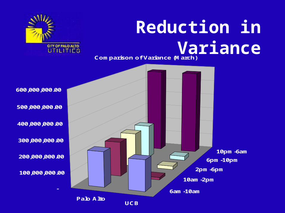
Reduction in Variance

Palo AltoUCB

6am-10am

10am-2pm

2pm-6pm

6pm-10pm

10pm-6am

-

100,000,000.00

200,000,000.00

300,000,000.00

400,000,000.00

500,000,000.00

600,000,000.00

Comparison of Variance (March)

Summary of Results

• UCB Model Savings– $1.121 million for 1998– 4% cost reduction

• UCB with revenue Model– additional $180,762 for 1998– additional 1% cost reduction

• Reduction in Variance

Benefits of UCB Model

• Utilizes all available procurement options

• Low Run-time • Partitions day into finer time

intervals– more closely follows demand curve– reduction in variance from actual load

• Reduction in risk

Recommendations

• Replace existing model with UCB model

• Negotiate with WAPA to reduce lower capacity limit– For June 1998, the max purchase quantity

is ~ 40 mwh (no lower capacity limit)

• Incorporate spot market into decisions