IEEE TRANSACTIONS ON VISUALIZATION AND …jteran/papers/GSSJT15.pdfOptimization Integrator for Large Time Steps ... is a diagonal lumped-mass matrix. Since we are interested ... mate

Optimization Integrator for Large Time StepsTheodore F. Gast, Craig Schroeder, Alexey Stomakhin, Chenfanfu Jiang, and Joseph M. Teran

Abstract—Practical time steps in today’s state-of-the-art simulators typically rely on Newton’s method to solve large systems of

nonlinear equations. In practice, this works well for small time steps but is unreliable at large time steps at or near the frame rate,

particularly for difficult or stiff simulations. We show that recasting backward Euler as a minimization problem allows Newton’s method

to be stabilized by standard optimization techniques with some novel improvements of our own. The resulting solver is capable of

solving even the toughest simulations at the 24Hz frame rate and beyond. We show how simple collisions can be incorporated directly

into the solver through constrained minimization without sacrificing efficiency. We also present novel penalty collision formulations for

self collisions and collisions against scripted bodies designed for the unique demands of this solver. Finally, we show that these

techniques improve the behavior of Material Point Method (MPM) simulations by recasting it as an optimization problem.

Index Terms—Computer graphics, three-dimensional graphics and realism, animation

Ç

1 INTRODUCTION

THE most commonly used time integration schemes inuse today for graphics applications are implicit methods.

Among these, backward Euler [1], [2], [3], [4], [5] or variantson Newmark methods [6], [7], [8] are the most common,though evenmore sophisticated schemes like BDF-2 [9], [10],implicit-explicit schemes [11], [12], or even the more exoticexponential integrators [13] have received consideration.Integrators have been the subject of comparison before (seefor example [3], [9], [14]), seeking good compromisesbetween speed, accuracy, robustness, and dynamic behavior.

These integrators require the solution to one or morenonlinear systems of equations each time step. These sys-tems are typically solved by some variation on Newton’smethod. Even the most stable simulators are typically runseveral time steps per 24Hz frame of simulation. There isgrowing interest in running simulations at larger time steps[15], so that the selection of Dt can be made based on otherfactors, such as damping or runtime, and not only onwhether the simulator works at all. One of the major factorsthat limits time step sizes is the inability of Newton’smethod to converge reliably at large time steps (SeeFigs. 3, 2, and 4), or if a fixed number of Newton iterationsare taken, the stability of the resulting simulation. Weaddress this by formulating our nonlinear system of equa-tions as a minimization problem, which we demonstratecan be solved more robustly. The idea that dynamics,energy, and minimization are related has been knownsince antiquity and is commonly leveraged in variational

integrators [6], [12], [16], [17], [18], [19], [20]. The idea thatthe nonlinear system that occurs from methods like back-ward Euler can be formulated as aminimization problem hasappearedmany times in graphics in various forms [2], [4], [5],[13], [19]. [19] point out that minimization leads to a methodthat is both simpler and faster than the equivalent nonlinearroot-finding problem, and [5] show that a minimization for-mulation can be used to solvemass-spring systemsmore effi-ciently. Kane et al. [17] use a minimization formulation as ameans of ensuring that a solution to their nonlinear systemcan be found assuming one exists. Goldenthal et al. [21]shows that aminimization formulation can be used to enforceconstraints robustly and efficiently. Hirotaet al. [2] shows thatsupplementing Newton’s method with a line search greatlyimproves robustness. Martin et al. [4] also shows thatsupplementing Newton’s method with a line search and adefiniteness correction leads to a robust solution procedure.Following their example, we show that recasting the solutionof the nonlinear systems that result from implicit time inte-gration schemes as a nonlinear optimization problem resultsin substantial robustness improvements. We also show thatadditional improvements can be realized by incorporatingadditional techniques like Wolfe condition line searcheswhich curve around collision bodies, conjugate gradientwith early termination on indefiniteness, and choosingconjugate gradient tolerances based on the current degree ofconvergence.

This publication is an extended version of [22] in whichwe have applied the optimization integrator approach tothe MPM snow simulator of [23]. This allows us to takemuch larger time steps than the original method and resultsin a significant speedup.

2 TIME INTEGRATION

The equations of motion for simulating solids are

_xx ¼ vv MM _vv ¼ ff ff ¼ ffðxx; vvÞ;

where ff are forces. As is common in graphics we assumeMMis a diagonal lumped-mass matrix. Since we are interested

� T.F. Gast, C. Schroeder, and C. Jiang are with the University of CaliforniaLos Angeles, Los Angeles, CA 90095.E-mail: {tfg, Craig}@math.ucla.edu, [email protected].

� A. Stomakhin is with the Research, Walt Disney Animation Studios,Burbank, CA. E-mail: [email protected].

� J.M. Teran is with the University of California Los Angeles, Los Angeles,CA 90095, and the Walt Disney Animation Studios, Burbank, CA.E-mail: [email protected].

Manuscript received 13 Nov. 2014; revised 7 July 2015; accepted 12 July 2015.Date of publication 21 July 2015; date of current version 4 Sept. 2015.Recommended for acceptance by E. Sifakis and V. Koltun.For information on obtaining reprints of this article, please send e-mail to:[email protected], and reference the Digital Object Identifier below.Digital Object Identifier no. 10.1109/TVCG.2015.2459687

IEEE TRANSACTIONS ON VISUALIZATION AND COMPUTER GRAPHICS, VOL. 21, NO. 10, OCTOBER 2015 1103

1077-2626� 2015 IEEE. Personal use is permitted, but republication/redistribution requires IEEE permission.See http://www.ieee.org/publications_standards/publications/rights/index.html for more information.

in robustness and large time steps, we follow a backwardEuler discretization. This leads to

xxnþ1 � xxn

Dt¼ vvnþ1 MM

vvnþ1 � vvn

Dt¼ ffnþ1 ¼ ffðxxnþ1; vvnþ1Þ:

Eliminating vvnþ1 yields

MMxxnþ1 � xxn � Dtvvn

Dt2¼ ff xxnþ1;

xxnþ1 � xxn

Dt

� �;

which is a nonlinear system of equations in the unknownpositions xxnþ1. This system of nonlinear equations is nor-mally solved with Newton’s method. If we define

hhðxxnþ1Þ ¼ MMxxnþ1 � xxn � Dtvvn

Dt2� ff xxnþ1;

xxnþ1 � xxn

Dt

� �; (1)

then our nonlinear problem is one of finding a solution tohhðxxÞ ¼ 00. To do this, one would start with an initial guess

xxð0Þ, such as the value predicted by forward Euler. This esti-mate is then iteratively improved using the update rule

xxðiþ1Þ ¼ xxðiÞ � @hh

@xxðxxðiÞÞ

� ��1

hhðxxðiÞÞ:

Each step requires the solution of a linear system, which isusually symmetric and positive definite and solved with aKrylov solver such as conjugate gradient or MINRES.

If the function hhðxxÞ is well-behaved and the initialguess sufficiently close to the solution, Newton’s methodwill converge very rapidly (quadratically). If the initialguess is not close enough, Newton’s method may con-verge slowly or not at all. For small enough time steps,the forward and backward Euler time steps will be very

similar (they differ by OðDt2Þ), so a good initial guess isavailable. For large time steps, forward Euler will beunstable, so it will not provide a good initial guess. Fur-ther, as the time step grows larger, Newton’s methodmay become more sensitive to the initial guess (seeFig. 1). The result is that Newton’s method will often failto converge if the time step is too large. Figs. 2, 3, and 4show examples of simulations that ought to be routinebut where Newton fails to converge at Dt ¼ 1=24 s.

Sometimes, only one, or a small fixed number, of Newtonsteps are taken rather than trying to solve the nonlinearequation to a tolerance. The idea is that a small number ofNewton steps is sufficient to get most of the benefit fromdoing an implicit method while limiting its cost. Indeed,even a single Newton step with backward Euler can allowtime steps orders of magnitude higher than explicit meth-ods. Linearizing the problem only goes so far, though, andeven these solvers tend to have time step restrictions fortough problems.

2.1 Assumptions

We have found that when trying to be very robust,assumptions matter. Before introducing our formulationin detail, we begin by summarizing some idealized

Fig. 3. Cube being stretched: initial configuration (left), our method att ¼ 0:4 s and t ¼ 3:0 s (middle), and standard Newton’s method att ¼ 0:4 s and t ¼ 3:0 s (right). Both simulations were run with one timestep per 24Hz frame. Newton’s method requires three time steps perframe to converge on this simple example.

Fig. 2. Cube being stretched and then given a small compressive pulse,shown with our method (top) and standard Newton’s method (bottom).Both simulations were run with one time step per 24Hz frame. In this sim-ulation, Newton’s method is able to converge during the stretch phase,but a simple pulse of compression, as would normally occur due to a colli-sion, causes it to fail to converge and never recover. Newton’s methodrequires five time steps per frame to converge on this simple example.

Fig. 4. Two spheres fall and collide with one another with Dt ¼ 1=24 s: ini-tial configuration (left), our method (top), and Newton’s method (bottom).Notice the artifacts caused by Newton not converging. Newton’s methodrequires six time steps per frame to converge on this example.

Fig. 1. Convergence of Newton’s method (middle) and our stabilizedoptimization formulation (bottom) for a simple 36-dof simulation in 2D.The initial configuration (top) is parameterized in terms of a pixel loca-tion, with the rest configuration occurring at ð35 ; 12Þ. Initial velocity is zero,and one time step is attempted. Time steps are (left to right) 170, 40, 20,10, and 1 steps per 24Hz frame, with the rightmost image beingDt ¼ 1 s. Color indicates convergence in 0 iterations (black), 15 iterations(blue), 30 or more iterations (cyan), or failure to converge in 500 itera-tions (red). Note that Newton’s method tends to converge rapidly or notat all, depending strongly on problem difficulty and initial guess.

1104 IEEE TRANSACTIONS ON VISUALIZATION AND COMPUTER GRAPHICS, VOL. 21, NO. 10, OCTOBER 2015

assumptions we will make. In practice, we will relaxsome of these as we go along.

A1: Masses are positiveA2: ff ¼ � @F

@xx for some function FA3: F is bounded from belowA4: F is C1

Assumption (A1) implies that MM is symmetric and posi-tive definite and is useful for theoretical considerations;scripted objects violate this assumption, but they do notcause problems in practice.

Conservative forces always satisfy assumption (A2), andmost practical elastic force models will satisfy this. We willshow in Section 4.2 that even some damping models can beput into the required form. Friction can be given an approxi-mate potential which is valid for small Dt (See [24]). Sinceour examples focus on taking larger time steps we addressthe problem by incorporating friction explicitly after theNewton solve.

Assumption (A3) is generally valid for constitutivemodels, with the global minimum occurring at the restconfiguration. Gravity is an important example of a forcethat violates this assumption. In Section 2.3, we show thatassumption (A3) can be safely relaxed to include forceslike gravity.

Assumption (A4) is a difficult assumption. Technically,this assumption is a show-stopper, since we know of noconstitutive model that is both robust and satisfies it every-where. To be practical, this must be immediately loosenedto C0, along with a restriction on the types of kinks that arepermitted in F. The practical aspects of this are discussed inSection 3.3.

2.2 Minimization Problem

The solution to making Newton’s method converge reli-ably is to recast the equation solving problem as anoptimization problem, for which robust and efficientmethods exist. In principle, that can always be done,since solving hhðxxÞ ¼ 00 is equivalent to minimizing khhðxxÞkassuming a solution exists. This approach is not veryconvenient, though, since it requires a global minimumof khhðxxÞk. Further minimization using Newton’s methodwould require the Hessian of khhðxxÞk, which involves thesecond derivatives of our forces. The standard approachonly requires first derivatives. What we really want is aquantity E that we can minimize whose second deriva-tives only require the first derivatives of our forces. Thatis, we need to integrate our system of nonlinear equationshhðxxÞ. Assumption (A2) allows us to do this. This way ofrecasting the problem also requires only a local mini-mum be found.

We can write (1) as

hhðxxÞ ¼ MMxx� xxn � Dtvvn

Dt2þ @F

@xx:

We note that if we set

x̂x ¼ xxn þ Dtvvn EðxxÞ ¼ 1

2Dt2ðxx� x̂xÞTMMðxx� x̂xÞ þF;

then we have hh ¼ @E@xx. If the required assumptions are met, a

global minimum of E always exists.1 By assumption (A4),

Eðxxnþ1Þ is smooth at its minima, so @E@xx ðxxnþ1Þ ¼ 00 or equiva-

lently hhðxxnþ1Þ ¼ 00.2 Any local minimum is a solution to ouroriginal nonlinear equation (1). Although we are now doingminimization rather than root finding, we are still solvingexactly the same equations. The discretization and dynam-ics will be the same, but the solver will be more robust. Inparticular, we are not making a quasistatic approximation.

2.3 Gravity

A graphics simulation would not be very useful withoutgravity. Gravity has the potential energy function �MMggTxx,where gg is the gravitational acceleration vector, but thisfunction is not bounded. An object can fall arbitrarily farand liberate a limitless supply of energy, though in practicethis fall will be stopped by the ground or some other object.Adding the gravity force to our nonlinear system yields

hhðxxÞ ¼ MMxx� xxn � Dtvvn

Dt2�MMggþ @F

@xx;

which can be obtained from the bounded minimizationobjective

EðxxÞ ¼ 1

2Dt2ðxx� x̂x� Dt2ggÞTMMðxx� x̂x� Dt2ggÞ þF:

A more convenient choice of E, and the one we use in prac-tice, is obtained by simply adding the effects of gravity

Fg ¼ �MMggTxx into F. Since all choices E will differ by a con-stant shift, this more convenient minimization objective willalso be bounded from below.

3 MINIMIZATION

The heart of our simulator is our algorithm for solving opti-mization problems, which we derived primarily from [25],though most of the techniques we apply are well-known.We begin by describing our method as it applies to uncon-strained minimization and then show how to modify it tohandle the constrained case.

3.1 Unconstrained Minimization

Our optimization routine begins with an initial guess, xxð0Þ.Each iteration consists of the following steps:

1)$Register active set

2) Compute gradientrE and HessianHH of E at xxðiÞ

3) Terminate successfully if krEk < t

4) Compute Newton step Dxx ¼ �HH�1rE5) Make sure Dxx is a downhill direction

1. Assumptions (A1) and (A3) ensure that E is bounded from below.Let B be a lower bound on F. Then, let L ¼ Fðx̂xÞ �Bþ 1 and V be the

region where 12Dt2

ðxx� x̂xÞTMMðxx� x̂xÞ � L. Note that V is a closed and

bounded ellipsoid centered at x̂x. E must have a global minimum whenrestricted to the set V since it is a continuous function on a closed andbounded domain. Outside V, we have EðxxÞ > LþB ¼ Eðx̂xÞ þ 1, sothat the global minimum inside V is in fact a global minimum over allpossible values of xx.

2. Relaxation of assumption (A4) is discussed in Section 3.3, whereF is allowed to have ridge-type kinks. Since these can never occur at arelative minimum, the conclusion here is unaffected.

GAST ET AL.: OPTIMIZATION INTEGRATOR FOR LARGE TIME STEPS 1105

6) Clamp the magnitude of Dxx to ‘ if kDxxk > ‘7) Choose step size a in direction Dxx using a line search8) Take the step: xxðiþ1Þ ¼ xxðiÞ þ aDxx9)

$Project xxðiþ1Þ.

Here, t is the termination criterion, which controls howaccurately the system must by solved. The length clamp ‘guards against the possibility of the Newton step being

enormous (if kDxxk ¼ 10100, computing FðxxðiÞ þ DxxÞ isunlikely to work well). Its value should be very large. Ourline search is capable of choosing a > 1, so the algorithm isvery insensitive with respect to the choice ‘. We normally

use ‘ ¼ 103. Steps beginning with$

are only performed forconstrained optimization and will be discussed later. A fewof the remaining steps require further elaboration here.

Linear solver considerations. Computing the Newton steprequires solving a symmetric linear system. The obviouscandidate solver for this is MINRES that can handle indefi-nite systems, and indeed this will work. However, there aremany tradeoffs to be made here. In contrast to a normalNewton solve, an accurate estimate for Dxx is not necessaryfor convergence. Indeed, we would still converge with highprobability if we chose Dxx to be a random vector. The pointof using the Newton direction is that convergence willtypically be much more rapid, particularly when the super-convergence of Newton’s method kicks in. (ChoosingDxx ¼ �rE leads to gradient descent, for example, whichcan display notoriously poor convergence rates.) When thecurrent estimate is far from the solution, the exact Newtondirection tends to be little better than a very approximateone. Thus, the idea is to spend little time on computing Dxxwhen krEk is large and more time when it is small. Wedo this by solving the system to a relative tolerance of

minð12 ; sffiffiffiffiffiffiffiffiffiffiffiffiffiffiffiffiffiffiffiffiffiffiffiffiffiffiffiffiffiffimaxðkrEk; tÞp Þ. The 1

2 ensures that we always

reduce the residual by at least a constant factor, which guar-antees convergence. The scale s adjusts for the fact that rEis not unitless (we usually use s ¼ 1). If our initial guess isnaive, we must make sure we take at least one minimizationiteration, even ifrE is very small. Using t here ensures thatwe do not waste time solving to a tiny tolerance in this case.

Conjugate gradient. One further optimization is to use con-jugate gradient as the solver with a zero initial guess. Ifindefiniteness is encountered during the conjugate gradientsolve, return the last iterate computed. If this occurs on thefirst step, return the right hand side. If this is done, Dxx isguaranteed to be a downhill direction, though it might notbe sufficiently downhill for our purposes. In practice, indefi-niteness will only occur if far from converged, in which caselittle time is wasted in computing an accurate Dxx that isunlikely to be very useful anyway. Indeed, if the systemis detectably indefinite and Dxx is computed exactly, itmight not even point downhill. Since we are searchingfor a minimum of E (even a local one), the Hessian of Ewill be symmetric and positive definite near this solution.(Technically, it need only be positive semidefinite, but inpractice this is of little consequence.) Thus, when we areclose enough to the solution for an accurate Newton stepto be useful, conjugate gradient will suffice to compute it.This is very different from the normal situation, where asolver like MINRES or an indefiniteness correction areemployed to deal with the possibility of indefiniteness.

In the case of our solver, neither strategy is necessary,and both make the algorithm slower.

Downhill direction. Making sure Dxx points downhill isfairly straightforward. If Dxx � rE < �kkDxxkkrEk, then weconsider Dxx to be suitable. Otherwise, if �Dxx is suitable, useit instead. If neither Dxx nor �Dxx are suitable, then we usethe gradient descent direction �rE. Note that if the conju-gate gradient strategy is used for computing the Newtondirection, then �Dxxwill never be chosen as the search direc-

tion at this stage. We have found k ¼ 10�2 to work well.Line search. For our line search procedure, we use an algo-

rithm for computing a such that the strongWolfe Conditionsare satisfied. See [25] for details. The line search procedureguarantees that E never increases from one iteration to thenext and that, provided certain conditions are met, sufficientprogress is always made. One important attribute of this linesearch algorithm is that it first checks to see if Dxx itself is asuitable step. In this way, the line search is almost entirelyavoided when Newton is converging properly.

Initial guess. A good initial guess is important for efficientsimulation under normal circumstances. Under low-Dt orlow-stress conditions, a good initial guess is obtained by

replacing ffnþ1 by ffn resulting in

MMxxð0Þ � xxn � Dtvvn

Dt2¼ ffðxxnÞ:

Solving for xxnþ1 yields the initial guess

xxð0Þ ¼ xxn þ Dtvvn þ Dt2MM�1ffðxxnÞ:

This initial guess is particularly effective under free fall,since here the initial guess is correct and no Newton itera-tions are required. On the other hand, this initial guess isthe result of an explicit method, which will be unstable atlarge time steps or high stress. Under these conditions, thisis unlikely to be a good initial guess and may in fact be veryfar from the solution. Under these situations, a better initialguess is obtained from xxð0Þ ¼ xxn þ Dtvvn. In practice, wecompute both initial guesses and choose the one which pro-duces the smaller value of E. This way, we get competitiveperformance under easy circumstances and rugged reliabil-ity under tough circumstances.

3.2 Constrained Minimization

We use constrained minimization for some of our collisions,which may result in a large active set of constraints, such aswhen an ball is bouncing on the ground.As the ball rises, con-straints become deactivated. As the ball hits the ground,moreconstraints become activated. The change in the number ofactive constraints from iteration to iteration may be quite sig-nificant. This would render a traditional active set methodimpractical, since constraints are activated or deactivated oneat a time. Instead, we use the gradient-projection method asour starting point, since it allows the number of active con-straints to change quickly. The downside to this choice is thatits reliance on the ability to efficiently project to the feasibleregion limits its applicability to simple collision objects.

Projections. Let P ðxxÞ be the projection that applies Pbp toxxp for all body-particle pairs ðb; pÞ that are labeled as activeor are violated (fbðxxpÞ < 0). Note that pairs such that


fbðxxpÞ ¼ 0 (as would be the case once projected) are consid-

ered to be touching but not violated. The iterates xxðiÞ

obtained at the end of each Newton step, as well as theinitial guess, are projected with P .

Register active set. Let E0 be the objective that would becomputed in the unconstrained case. The objective functionfor constrained optimization is EðxxÞ ¼ E0ðP ðxxÞÞ. Computethe gradient rE0. Constraints that are touching and forwhich rE0 � rfb � 0 are labeled as active for the remainderof the Newton step. All others are labeled as inactive. Noconstraint should be violated at this stage. Note that

E0ðxxðiÞÞ ¼ EðxxðiÞÞ is true before and after every Newtonstep, since constraints are never violated there.

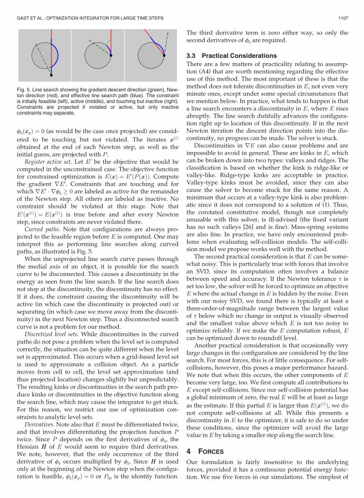
Curved paths. Note that configurations are always pro-jected to the feasible region before E is computed. One mayinterpret this as performing line searches along curvedpaths, as illustrated is Fig. 5.

When the unprojected line search curve passes throughthe medial axis of an object, it is possible for the searchcurve to be disconnected. This causes a discontinuity in theenergy as seen from the line search. If the line search doesnot stop at the discontinuity, the discontinuity has no effect.If it does, the constraint causing the discontinuity will beactive (in which case the discontinuity is projected out) orseparating (in which case we move away from the disconti-nuity) in the next Newton step. Thus a disconnected searchcurve is not a problem for our method.

Discretized level sets. While discontinuities in the curvedpaths do not pose a problem when the level set is computedcorrectly, the situation can be quite different when the levelset is approximated. This occurs when a grid-based level setis used to approximate a collision object. As a particlemoves from cell to cell, the level set approximation (andthus projected location) changes slightly but unpredictably.The resulting kinks or discontinuities in the search path pro-duce kinks or discontinuities in the objective function alongthe search line, which may cause the integrator to get stuck.For this reason, we restrict our use of optimization con-straints to analytic level sets.

Derivatives. Note also that E must be differentiated twice,and that involves differentiating the projection function Ptwice. Since P depends on the first derivatives of fb, theHessian HH of E would seem to require third derivatives.We note, however, that the only occurrence of the thirdderivative of fb occurs multiplied by fb. Since HH is usedonly at the beginning of the Newton step when the configu-ration is feasible, fbðxxpÞ ¼ 0 or Pbp is the identity function.

The third derivative term is zero either way, so only thesecond derivatives of fb are required.

3.3 Practical Considerations

There are a few matters of practicality relating to assump-tion (A4) that are worth mentioning regarding the effectiveuse of this method. The most important of these is that themethod does not tolerate discontinuities in E, not even veryminute ones, except under some special circumstances thatwe mention below. In practice, what tends to happen is thata line search encounters a discontinuity in E, where E risesabruptly. The line search dutifully advances the configura-tion right up to location of this discontinuity. If in the nextNewton iteration the descent direction points into the dis-continuity, no progress can be made. The solver is stuck.

Discontinuities in rE can also cause problems and areimpossible to avoid in general. These are kinks in E, whichcan be broken down into two types: valleys and ridges. Theclassification is based on whether the kink is ridge-like orvalley-like. Ridge-type kinks are acceptable in practice.Valley-type kinks must be avoided, since they can alsocause the solver to become stuck for the same reason. Aminimum that occurs at a valley-type kink is also problem-atic since it does not correspond to a solution of (1). Thus,the corotated constitutive model, though not completelyunusable with this solver, is ill-advised (the fixed varianthas no such valleys [26] and is fine). Mass-spring systemsare also fine. In practice, we have only encountered prob-lems when evaluating self-collision models. The self-colli-sion model we propose works well with the method.

The second practical consideration is that E can be some-what noisy. This is particularly true with forces that involvean SVD, since its computation often involves a balancebetween speed and accuracy. If the Newton tolerance t isset too low, the solver will be forced to optimize an objectiveE where the actual change in E is hidden by the noise. Evenwith our noisy SVD, we found there is typically at least athree-order-of-magnitude range between the largest valueof t below which no change in output is visually observedand the smallest value above which E is not too noisy tooptimize reliably. If we make the E computation robust, Ecan be optimized down to roundoff level.

Another practical consideration is that occasionally verylarge changes in the configuration are considered by the linesearch. For most forces, this is of little consequence. For self-collisions, however, this poses a major performance hazard.We note that when this occurs, the other components of Ebecome very large, too. We first compute all contributions toE except self-collisions. Since our self-collision potential hasa global minimum of zero, the real E will be at least as large

as the estimate. If this partial E is larger than EðxxðiÞÞ, we donot compute self-collisions at all. While this presents adiscontinuity in E to the optimizer, it is safe to do so underthese conditions, since the optimizer will avoid the largevalue inE by taking a smaller step along the search line.

4 FORCES

Our formulation is fairly insensitive to the underlyingforces, provided it has a continuous potential energy func-tion. We use five forces in our simulations. The simplest of

Fig. 5. Line search showing the gradient descent direction (green), New-ton direction (red), and effective line search path (blue). The constraintis initially feasible (left), active (middle), and touching but inactive (right).Constraints are projected if violated or active, but only inactiveconstraints may separate.


these is gravity, which we addressed in Section 2.2. We alsoemploy a hyperelastic constitutive model (Section 4.1), aRayleigh damping model (Section 4.2), and two collisionpenalty force models (Sections 5.2 and 5.3).

4.1 Elastic

A suitable hyperelastic constitutive model must have afew key properties to be suitable for this integrator. Themost important is that it must have a potential energyfunction defined everywhere, and this function must becontinuous. The constitutive model must be well-definedfor any configuration, including configurations that aredegenerate or inverted. This is true even if objects do notinvert during the simulation, since the minimization pro-cedure may still encounter such states. Examples of suit-able constitutive models are those defined by thecorotated hyperelasticity energy [27], [28], [29], [30], [31],[32] (but see Section 3.3), and the fixed corotated hypere-lasticity variant [26]. Stress-based extrapolated models[33], [34] are unsuitable due to the lack of a potentialenergy function in the extrapolated regime, but energy-based extrapolation models [26] are fine. We use the fixedcorotated variant [26] for all of our simulations for itscombination of simplicity and robustness.

4.2 Damping

At first, one might conclude that requiring a potentialenergy may limit our method’s applicability, since dampingforces cannot be defined by a potential energy function. Avery simple damping model is given by ff ¼ �kMMvvnþ1.Eliminating the velocity from the equation yields

ffðxxnþ1Þ ¼ �kMMxxnþ1 � xxn

Dtðk > 0Þ:

The scalar function

Fðxxnþ1Þ ¼ k

2Dtðxxnþ1 � xxnÞTMMðxxnþ1 � xxnÞ

has the necessary property that ff ¼ � @F@xx. Note that this F

looks very similar to our inertial term in E, and it is simi-larly bounded from below. That this F is not a real potentialenergy function is evident from its dependence on xxn andDt, but it is nevertheless suitable for use in our integrator.This simple drag force is not very realistic, though, so we donot use it in our simulations.

A more realistic damping force is Rayleigh damping. Letc be an elastic potential energy function. The stiffness

matrix corresponding to this force is� @2c@xx@xx, and the Rayleigh

damping force and associated objective are

ff ¼ �k@2c

@xx@xxðxxnþ1Þ

� �vvnþ1 Fc ¼ k

Dtðxxnþ1 � xxnÞT @c

@xx� c

� �:

This candidate Fc has at least two serious problems. Thefirst is that second derivatives of Fc involve third deriva-

tives of c. The second is that @2c@xx@xx may be indefinite, in

which case the damping force may not be entirelydissipative. Instead, we approximate Rayleigh damping

with a lagged version. Let DD ¼ @2c@xx@xx ðxxnÞ. Since DD does not

depend on xxnþ1, the lagged Rayleigh damping force

and associated objective are

ff ¼ �kDDvvnþ1 Fd ¼ k

2Dtðxxnþ1 � xxnÞTDDðxxnþ1 � xxnÞ:

This solves the first problem, since the second derivative of

Fd is just kDt DD. Since DD is not being differentiated, it is safe

to modify it to eliminate indefiniteness as described in [26],[34]. This addresses the second problem. We did not use the

damping model found in [35], which uses cðxxnþ1Þ with xxn

used as the rest configuration, because it is not definedwhen xxn is degenerate.

5 COLLISIONS

Collisions are a necessary part of any practical computergraphics simulator. The simplest approach to handlingcollisions is to process them as a separate step in the timeintegration scheme. This works well for small time steps,but it causes problems when used with large time stepsas seen in Fig. 10. Such arrangement often leads to thecollision step flattening objects to remove penetration andthe elastic solver restoring the flattened geometry bypushing it into the colliding object. To get around thisproblem, the backward Euler solver needs to be aware ofcollisions. A well-tested strategy for doing this is to usepenalty collisions, and we do this for two of our threecollision processing techniques. Our other approach is toadd position constraints to the nonlinear solve.

Fig. 11 uses constraints for all collision body collisionsand demonstrates that our constraint collisions are effec-tive with concave and convex constraint manifolds. Fig. 13demonstrates our constraint collisions are effective forobjects with sharp corners. Fig. 7 is a classical torus dropdemonstrating that our self collisions are effective at stop-ping collisions at the torus’s hole. Fig. 12 demonstrates ourself collisions method with stiffer deformable bodies withsharp corners. Finally, Fig. 9 shows a more practical exam-ple which uses all three types of collisions: self collisions,constraint collisions (with ground) and penalty collisions(against a bowl defined by a grid-based level set).

5.1 Object Collisions As Constraints

Our first collision processing technique takes advantageof our minimization framework to treat collisions withnon-simulated objects as inequality constraints. Treatingcollisions or contacts as constraints is not new and infact forms the basis for LCP formulations such as [36],[37]. Unlike LCP formulations, however, our formulationdoes not attempt to be as complete and as a resultcan be solved about as efficiently as a simple penaltyformulation.

Our constraint collision formulation works reliably whenthe level set is known analytically. This limits its applicabil-ity to analytic collision objects. While this approach is feasi-ble only under limited circumstances, these circumstancesoccur frequently in practice. When this approach is applica-ble, it is our method of choice, since it produces betterresults (e.g., no interpenetration) for similar cost. Whenthis formulation is not applicable, we use a penalty collisionformulation instead.


We begin by representing our collision objects (indexedwith b) by a level set, which we denote fb to avoid confusionwith potential energy. By convention, fbðxxÞ < 0 for points xxin the interior of the collision object b. Our collision con-

straint is simply that fbðxxnþ1p Þ � 0 for each simulation

particle p and every constraint collision object b. With such aformulation, we can project a particle at xxp to the closestpoint xx0

p on the constraint manifold using

xx0p ¼ PbpðxxpÞ ¼ xxp � fbðxxpÞrfbðxxpÞ:

We show how to solve the resulting minimization problemin Section 3.2.

We apply friction after the Newton solve. The total colli-sion force felt by particles is

Dtffcol ¼ rE0ðxxnþ1Þ � rEðxxnþ1Þ ¼ rE0ðxxnþ1Þ � rE0ðP ðxxnþ1ÞÞ;where E0 is the objective in the absence of constraints (SeeSection 3.2). Only collision pairs that are active at the end ofthe minimization will be applying such forces. We use thelevel set’s normal and the collision force to apply Coulombfriction to colliding particles. In particular, we use the rule

(vvnþ1p ! v̂vnþ1

p )

nn ¼ rf vvnþ1p;n ¼ nn � vvnþ1

p

� �nn vvnþ1

p;t ¼ vvnþ1p � vvnþ1

p;n

v̂vnþ1p ¼ vvnþ1

p;n þmax 1� mDtðnn � ffp;colÞmkvvp;tk ; 0

� �vvnþ1p;t :

Our constraint collision formulation is not directly appli-cable to grid-based level sets, since we assume thatPbpðPbpðxxpÞÞ ¼ PbpðxxpÞ and PbpðxÞ is continuous. Continuity

of PbpðxÞ can be achieved, for example, with C1 cubic splinelevel set interpolation. However, it will not generally betrue that PbpðPbpðxxpÞÞ ¼ PbpðxxpÞ. Alternatively, the projectionroutine can be modified to iterate the projection to conver-gence, but then continuity is lost.

5.2 Object Penalty Collisions

When a collision object is not analytic, as will normallybe the case for characters for instance, we use a penaltyformulation instead. As in the constraint formulation, weassume our collision object is represented by a level setfb. The elastic potential energy FbpðxxpÞ of our penalty

force is FbpðxxÞ ¼ 0 if fbðxxpÞ > 0 and FbpðxxpÞ ¼ kfbðxxpÞ3otherwise. Since Fbp is a potential energy, we must dif-ferentiate it twice for our solver. It is important to com-pute the derivatives of fb exactly by differentiating theinterpolation routine rather than approximating them

using central differences. While a C1 cubic spline inter-polation is probably a wiser interpolation strategy sinceit would avoid the energy kinks that may be caused by apiecewise linear encoding of the level set, we found lin-ear interpolation to work well, too, and we use linearinterpolation in our examples.

As in the constraint case, we apply friction after the New-ton solve. The total collision force felt by a particle due toobject penalty collisions is obtained by evaluating the pen-alty force at xxnþ1 and using this force as the normal direc-tion. That is,

ffcol ¼ � @Fbp

@xxðxxnþ1Þ fp;n ¼ kffp;colk nn ¼ ffp;col

fp;n

vvnþ1p;n ¼ nn � vvnþ1

p

� �nn vvnþ1

p;t ¼ vvnþ1p � vvnþ1

p;n

v̂vnþ1p ¼ vvnþ1

p;n þmax 1� mDtfp;nmkvvp;tk ; 0

� �vvnþ1p;t :

5.3 Penalty Self-Collisions

We detect self-collisions by performing point-tetrahedroninclusion tests, which we accelerate with a bounding boxhierarchy. If a point is found to be inside a tetrahedron butnot one of the vertices of that tetrahedron, then we flag theparticle as colliding.

Once we know a particle is involved in a self collision, weneed an estimate for how close the particle is to the bound-ary. If this particle has collided before, we use the primitiveit last collided with as our estimate. Otherwise, we computethe approximate closest primitive in the rest configurationusing a level set and use the current distance to this surfaceelement as an estimate.

Given this upper bound estimate of the distance to theboundary, we perform a bounding box search to conser-vatively return all surface primitives within that distance.We check these candidates to find the closest one. Nowwe have a point-primitive pair, where the primitive is thesurface triangle, edge, or vertex that is closest to the pointbeing processed. Let d be the square of the point-primi-tive distance. The penalty collision energy for this point is

F ¼ kdffiffiffiffiffiffiffiffiffiffiffidþ �

p, where � is a small number (10�15 in our

case) to prevent the singularities when differentiating.Note that this penalty function is approximately cubic inthe penetration depth. This final step is the only part thatmust be differentiated.

As with the other two collision models, we apply fric-tion after the Newton solve. In the most general case, apoint n0 collides with a surface triangle with vertices n1,n2, and n3. As with the object penalty collision model, col-

lision forces are computed by evaluating Fðxxnþ1Þ and itsderivative. The force applied to n0 is denoted ff ; its direc-tion is taken to be the normal direction nn. The closestpoint on the triangle to n0 has barycentric weights w1, w2,

and w3. Let w0 ¼ �1 for convenience. Let QQ ¼ II � nnnnT ,

noting than QQ2 ¼ QQ. If we apply a tangential impulse QQjjto these particles, their new velocities and kinetic energywill be

v̂vnþ1ni

¼ vvnþ1ni

þ wim�1niQQjj KE ¼

X3n¼0

1

2mni v̂vnþ1

ni

� �T

v̂vnþ1ni

:

We want to minimize this kinetic energy to prevent frictionfrom causing instability. Since M is positive definite, we seethatKE is minimized when

rKE ¼ QQvvþm�1QQjj ¼ 0vv ¼X3n¼0

wivvnþ1ni

m�1 ¼X3n¼0

wim�1niwi:

If we let jj ¼ �mQQvv then rKE ¼ 0 and QQjj ¼ jj. This leads tothe friction application rule


v̂vnþ1ni

¼ vvnþ1ni

þ wim�1nimin

mkffkkjjk ; 1

� �jj:

Note that all three friction algorithms decrease kineticenergy but do not modify positions, so none of them canadd energy to the system, and thus stability ramificationsare unlikely even though friction is applied explicitly.This approach to friction can have artifacts, however,since friction will be limited to removing kinetic energyfrom colliding particles. This limits the amount of frictionthat can be applied at large time steps. An approach simi-lar to the one in [36] that uses successive Quadratic Pro-gramming solves could possibly be applied to eliminatethese artifacts. However [38] found existing large-scalesparse QP solvers to be insufficiently robust, and thus wedid not use this method.

6 ACCELERATING MATERIAL POINT METHOD

(MPM)

In this section we describe the application of this optimi-zation approach to the snow simulation from [23]. Theirapproach to simulating snow uses the material pointmethod, a hybrid Eulerian-Lagrangian formulation thatuses unstructured particles as the primary representationand a background grid for applying forces. They used anenergy-based formulation to facilitate a semi-implicittreatment of MPM. While this leads to a significant timestep improvement over more standard explicit treat-ments, it still requires a small time step in practice toremain stable. We show how to modify their original for-mulation so that we are able to take time steps on theorder of the CFL condition. We also provide an improvedtreatment of collisions with solid bodies that naturallyhandles them as constraints in the optimization.Although the optimization solve is for grid velocities, weshow that a backward Euler (rather than forward Euler)update of particle positions in the grid based velocityfield automatically guarantees no particles penetratesolid bodies. In addition to the significantly improvedstability, we demonstrate in Section 7.1 that in manycases a worthwhile speedup can be obtained with ournew formulation.

6.1 Revised MPM Time Integration

In [23, Section 4.1], the original method is broken down into10 steps. From the original method, Steps 3-6 and 9-10 aremodified. We begin by summarizing these steps as theyapply to our optimization-based MPM integrator.

1) Rasterize particle data to the grid. First, mass and

momentum are transferred from particles to the grid

using mnii ¼ P

p mpwniip and mn

ii vvnii ¼ P

p vvnpmpw

niip.

Velocity is then obtained by division usingvvnii ¼ mn

ii vvnii =m

nii . Transferring velocity in this way

conserves momentum.2) Compute particle volumes. First time step only. Our

force discretization requires a notion of a particle’svolume in the initial configuration. Since cells havea well-defined notion of volume and mass, we canestimate a cell’s density as r0ii ¼ m0

ii =h3 and

interpolate it back to the particle as r0p ¼P

ii r0iiw

0iip.

Finally, we can define a particle’s volume to be

V 0p ¼ mp=r

0p. Though rather indirect, this approach

automatically provides an estimate of the amountof volume that can be attributed to individualparticles.

3) Solve the optimization problem. Minimize the objective(2) using the methods of Section 3. This produces anew velocity estimate vvnþ1

ii on the grid. This stepreplaces Steps 3-6 of the original method.

4) Update deformation gradient. The deformation gradi-ent for each particle is updated as FFnþ1

p ¼ ðIIþDtrvvnþ1

p ÞFFnp , where we have computed rvvnþ1

p ¼Pii vv

nþ1ii ðrwn

iipÞT . Note that this involves updates for

the elastic and plastic parts of FF . See [23] for details,as they are unchanged.

5) Update particle velocities. Our new particle velocitiesare vvnþ1

p ¼ ð1� aÞvvnþ1PICp þ avvnþ1

FLIPp, where the PIC

part is vvnþ1PICp ¼

Pii vv

nþ1ii wn

iip and the FLIP part is

vvnþ1FLIPp ¼ vvnp þ

Piiðvvnþ1

ii � vvnii Þwniip. We typically used

a ¼ 0:95.6) Update particle positions. Particle positions are

updated using xxnþ1p ¼ xxn

p þ Dtvvðxxnþ1p Þ as described in

Section 6.3. This step replaces steps 9-10 of the origi-nal method.

6.2 Optimization Formulation

The primary modification that we propose is to use theoptimization framework in place of the original solver.For this, we must formulate their update in terms ofan optimization objective E. The original formulationdefined the potential energy FðxxiiÞ conceptually in termsof the grid node locations xxii. Here we use the index ii torefer to grid node indices. Their grid is a fixed Cartesian

grid and never moves, and they solve for vvnþ1ii . We will

follow the same conceptual formulation here. This leadsto the objective

EðvviiÞ ¼Xii

1

2miikvvii � vvnii k2 þF xxn

ii þ Dtvvii� �

; (2)

where mii is the mass assigned to grid index ii. Our final

vvnþ1ii is computed so that Eðvvnþ1

ii Þ is minimized. We solvethis minimization problem as in Section 3. Note that weapply plasticity explicitly as in the original formulation.

Using larger time steps causes our linear systems tobecome slower to solve. In the case of MPM, we found itbeneficial to use the diagonal preconditioner

LLiiii ¼Xp

diag mpwiipII þ Dt2V 0p HH

� �;

where

HH ¼ ð�p þ mpÞrwiiprwTiip þ mprwT

iiprwiipII:

This preconditioner approximates the diagonal of the stiff-ness matrix at the rest configuration. This works well sincesnow is unable to deform much without hardening or frac-turing. We use an approximation to the diagonal, rather


than the exact diagonal, because we never explicitly formthe matrix. This approximation suffices for preconditioningand is more efficient.

The original method performed solid body collisionswhile computing new grid velocities. We treat body col-lisions using constraints in our optimization problem.We assume sticking collisions and let P ðvviiÞ ¼ 00 for allgrid nodes ii that lie inside a collision object. Note thatwe do not permit separation during optimization,though separation may occur during other steps in thealgorithm.

6.3 Particle Position Update

One of the difficulties with running the method of [23] withlarger time steps is the particle-based solid body collisions.They were needed under the old formulation to prevent set-tling into the ground, but at the same time they causebunching of particles at collision objects. These problemsare exacerbated at larger time steps, and another approachis required. Instead, we show that altering the way weupdate particle positions can avoid the need for a separateparticle collision step.

For each particle position xxp we solve the backward Eulerupdate equation

xxnþ1p ¼ xxnp þ Dtvv xxnþ1

p

� �vvðxxnþ1

p Þ ¼Xii

vvnþ1ii Nh

ii ðxxpÞ;

where vvðxxnþ1p Þ is the interpolated grid velocity at the par-

ticle location xxnþ1p . These updates are independent per

particle and so are relatively inexpensive. A solution tothis backward Euler equation always exists nearby pro-vided a suitable CFL condition is respected (no particlemoves more than Dxx in a time step). Note that pure PICvelocities are used in the particle position updates. Whilea combination of FLIP/PIC is still stored on particles (toavoid excessive dissipation in subsequent transfer togrid), PIC velocities for position updates lead to morestable behavior.

The motivation for our modification can be best under-stood in the case of sticking collisions. Inside a collisionobject, we will have vvnþ1

ii ¼ 00 due to the collision constraintsimposed during optimization. If we then assume that we

will interpolate vvðxxnþ1p Þ ¼ 00 here, then we can see from

xxnþ1p ¼ xxn

p þ Dtvvðxxnþ1p Þ that xxnþ1

p ¼ xxnp . Note that if a particle

ends up inside the collision object, then it must have alreadybeen there. Thus, it is not possible for particles to penetrate

collision objects. In our implementation, vvðxxnþ1p Þ ¼ 00 will

only be true if we are slightly inside collision objects, but inpractice this procedure actually stops particles slightly out-side collision objects.

We solve this equation with Newton’s method. SinceNewton’s method need not converge, some care isrequired, though in practice nothing as sophisticated asSection 3 is needed. We always use the Newton directionbut repeatedly halve the length of the Newton stepuntil the objective E ¼ kxxnþ1

p � xxnp � Dtvvðxxnþ1

p Þk no longerincreases. (If halving the step size 14 times does not suf-fice, we take the reduced step anyway.) Typically, onlyone Newton step is required for convergence. We havenever observed this to fail.

We use a quadratic spline rather than the cubic ofthe original formulation to reduce stencil width andimprove the effectiveness of the modified positionupdate. That is, we let

NðxÞ ¼�x2 jxj < 1

2 ;12x

2 � 32 jxj þ 9

812 � jxj < 3

2 ;0 jxj � 3

2 :

8<:

Using a quadratic stencil also has the advantage of beingmore efficient. We do not use a linear spline since it is notsmooth enough for Newton’s method to be effective in theparticle position update.

Since MPM involves a grid, we limit our time step so thatparticles do not travel more that one grid spacing per timestep. That is, we choose Dt so that n Dxx

Dt � maxpkvvnpk forsome n < 1. We chose n ¼ 0:6 for our examples. Althoughthe time step restriction is computed based on vvnp rather

than vvnþ1p , this suffices in practice.

7 RESULTS

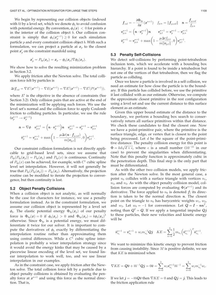
We begin by demonstrating how robust our solver is byconsidering the two most difficult constitutive modeltests we are aware of: total randomness and total degen-eracy. The attributes that make them tough constitutivemodel tests also make them tough solver tests: highstress, terrible initial guess, tangled configurations, andthe need to dissipate massive amounts of unwantedenergy. Fig. 6 shows the recovery of a 65� 65� 65 cube(824k dofs) from a randomized initial configuration for

Fig. 7. A torus falls on the ground (constraint collisions) and collides with itself (penalty collisions).

Fig. 6. Random test with 65� 65� 65 particles simulated withDt ¼ 1=24 s for three stiffnesses: low stiffness recovering over 100 timesteps (top), medium stiffness recovering over 40 time steps (bottomleft), and high stiffness recovering in a single time step (bottom right).The red tetrahedra are inverted, while the green are uninverted.


three different stiffnesses with Dt ¼ 1=24 s. Fig. 8 repeatsthe tests with all points starting at the origin. The recov-ery times vary from about 3 s for the softest to a singletime step for the stiffest. We were surprised to find thata single step of backward Euler could untangle a ran-domized cube, even at high resolution.

7.1 MPM Results

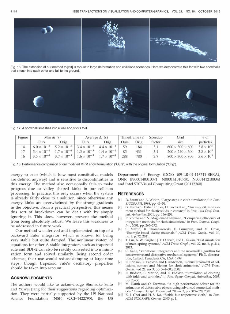
We demonstrate the advantages of using our optimiza-tion integrator by applying it to the MPM snow formula-tion from [23]. We run three examples using both theoriginal formulation and our modified formulation. Wecompare with the snowball examples from the originalpaper. In each case, for our formulation we use the CFLn ¼ 0:6. Fig. 17 shows a snowball hitting a wall usingsticky collisions, which causes the snow to stick to thewall. Fig. 14 shows a dropped snowball hitting theground with sticky collisions. Fig. 16 shows two snow-balls colliding in mid air with sticky collisions againstthe ground. On average, we get a speed up of 3.5 timesover the original method. These results are tabulated in

Fig. 18. Notably, we are able to take significantly largertime steps, however some of the potential gains fromthis are lost to an increased complexity per time step.Nonetheless, we provide a significant computational sav-ings with minimal modification to the original approach.

8 CONCLUSIONS

We have demonstrated that backward Euler solved withNewton’s method can be made more robust by recastingthe resulting system of nonlinear equations as a nonlinearoptimization problem so that robust optimization techni-ques can be employed. The resulting method is extremelyrobust to large time step sizes, high stress, and tangledconfigurations.

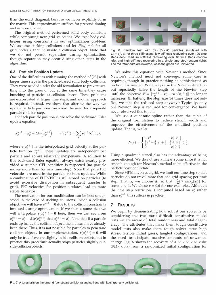
Fig. 8. Point test with 65� 65� 65 particles simulated with Dt ¼ 1=24 sfor three stiffnesses: low stiffness recovering over 120 time steps (top),medium stiffness recovering in five time steps (bottom left), and highstiffness recovering in a single time step (bottom right).

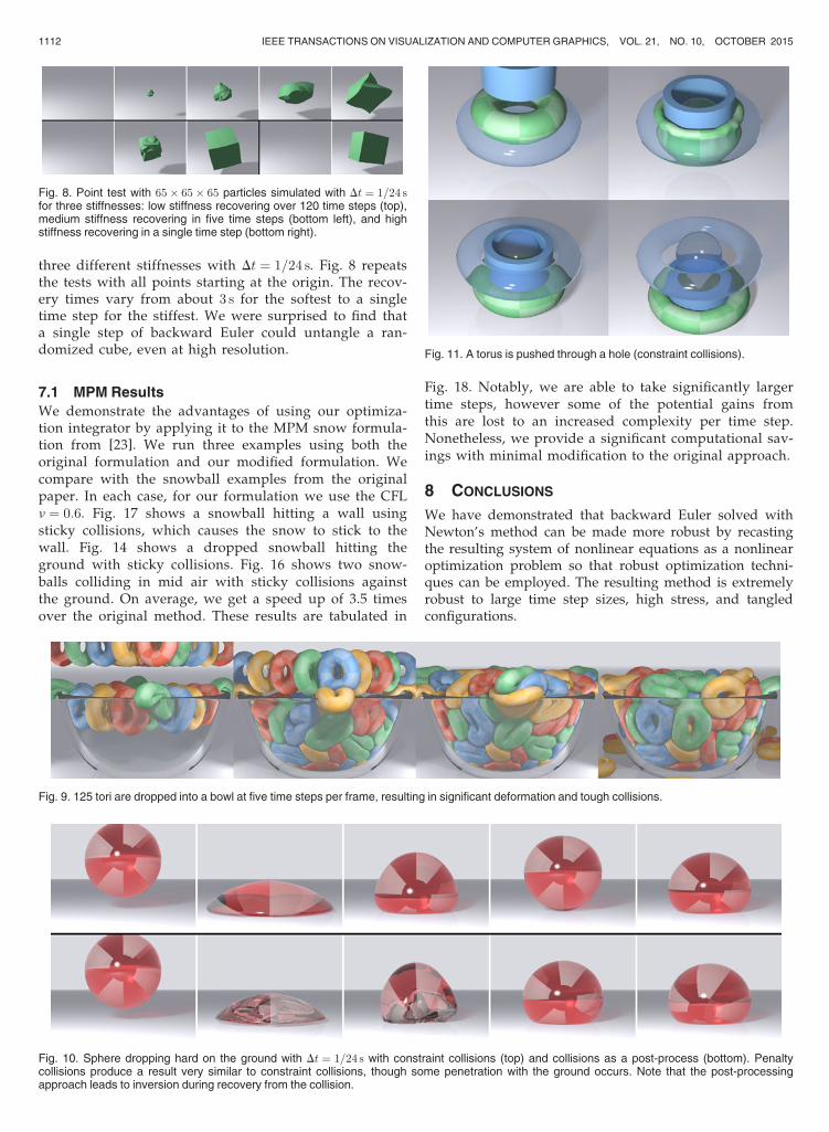
Fig. 9. 125 tori are dropped into a bowl at five time steps per frame, resulting in significant deformation and tough collisions.

Fig. 10. Sphere dropping hard on the ground with Dt ¼ 1=24 s with constraint collisions (top) and collisions as a post-process (bottom). Penaltycollisions produce a result very similar to constraint collisions, though some penetration with the ground occurs. Note that the post-processingapproach leads to inversion during recovery from the collision.

Fig. 11. A torus is pushed through a hole (constraint collisions).


Runtimes and other performance-related information forall of our sims are provided in Fig. 15. All Lagrangian simu-lations were run single-threaded on a 3:1-3:5GHz Xeoncore, the MPM simulations were run with 10 threads forFig. 16 and 12 threads for Fig. 14 and 17. Our solver’s perfor-mance is competitive with a standard Newton solver forthose examples where both were run. In general, we takemore Newton steps but spend less time on each, and theresulting runtime for typical examples is about the same forthe two solvers, though our solver is faster for all of the dif-ficult examples in this paper. Taking a large time step size

can actually be slower than taking a smaller one, even withthe same solver. For time integrators (like backward Euler)that have a significant amount of damping at large timesteps, constitutive models are often tuned to take intoaccount the numerical damping. If the integrator is forcedto simulate a portion of a simulation at a smaller time step,the dynamic behavior can change noticeably. Solving withconstraints is about the same speed as using penaltycollisions.

Note that Figs. 9 and 7 were run with smaller timesteps sizes to avoid collision artifacts. This indicates thata self-collision scheme that is more tolerant of large timesteps is required. The scheme does not have problemswith collisions between different objects at the frame rateas long as they are not too thin. Continuous collisiondetection could perhaps be used. We leave both of theseproblems for future work.

The current method has a couple disadvantages com-pared with current techniques. It requires a potential

Fig. 12. A stack of deformable boxes of varying stiffness is struck witha rigid kinematic cube (constraint collisions) with Dt ¼ 1=24 s. Thegreen boxes are 10 times as stiff as the blue boxes.

Fig. 13. An armadillo is squeezed between 32 rigid cubes (constraint col-lisions) with Dt ¼ 1=24 s. When this torture test is run at one, two, fourand eight steps per frame the average runtime per frame is 46, 58, 88,and 117 seconds respectively.

Fig. 14. Our approach works naturally with the material point method simulations from [23]. Here we demonstrate with a snowball that drops to theground and fractures. Notably, we provide a new treatment of particle position updates that naturally prevents penetration in solid objects like theground.

Fig. 15. Time step sizes and average running times for the examples inthe paper. The last column shows the average number of linear solvesper time step. Each of the Newton’s method examples fails to convergeat the frame rate. For fairer comparison, timing information for all but theone marked � is shown at the frame rate and the stable time step size.The stress tests marked þ spend the majority of their time on the firstframe or two due to the difficult initial state.


energy to exist (which is how most constitutive modelsare defined anyway) and is sensitive to discontinuities inthis energy. The method also occasionally fails to makeprogress due to valley shaped kinks in our collisionprocessing. In practice, this only occurs when the systemis already fairly close to a solution, since otherwise anyenergy kinks are overwhelmed by the strong gradientsin the objective. From a practical perspective, this meansthis sort of breakdown can be dealt with by simplyignoring it. This does, however, prevent the methodfrom being absolutely robust. We leave this weakness tobe addressed in future work.

Our method was derived and implemented on top of abackward Euler integrator, which is known for beingvery stable but quite damped. The nonlinear system ofequations for other A-stable integrators such as trapezoidrule and BDF-2 can also be readily converted into minimi-zation form and solved similarly. Being second orderschemes, their use would reduce damping at large timesteps, though trapezoid rule’s oscillatory propertiesshould be taken into account.

ACKNOWLEDGMENTS

The authors would like to acknowledge Shunsuke Saitoand Yuwei Jiang for their suggestions regarding optimiza-tion. They were partially supported by the US NationalScience Foundation (NSF) (CCF-1422795), the US

Department of Energy (DOE) (09-LR-04-116741-BERA),ONR (N000140310071, N000141010730, N000141210834)and Intel STCVisual Computing Grant (20112360).

REFERENCES

[1] D. Baraff and A. Witkin, “Large steps in cloth simulation,” in Proc.SIGGRAPH, 1998, pp. 43–54.

[2] G. Hirota, S. Fisher, C. Lee, H. Fuchs et al.,, “An implicit finite ele-ment method for elastic solids in contact,” in Proc. 14th Conf. Com-put. Animation, 2001, pp. 136–254.

[3] P. Volino and N. Magnenat-Thalmann, “Comparing efficiency ofintegration methods for cloth simulation,” in Proc. Comput. Graph.Int., 2001, pp. 265–272.

[4] S. Martin, B. Thomaszewski, E. Grinspun, and M. Gross,“Example-based elastic materials,” ACM Trans. Graph., vol. 30,no. 4, p. 72, 2011.

[5] T. Liu, A. W. Bargteil, J. F. O’Brien, and L. Kavan, “Fast simulationof mass-spring systems,” ACM Trans. Graph., vol. 32, no. 6, p. 214,2013.

[6] C. Kane, “Variational integrators and the newmark algorithm forconservative and dissipative mechanical systems,” Ph.D. disserta-tion, Caltech, Pasadena, CA, USA, 1999.

[7] R. Bridson, R. Fedkiw, and J. Anderson, “Robust treatment of col-lisions, contact and friction for cloth animation,” ACM Trans.Graph., vol. 21, no. 3, pp. 594–603, 2002.

[8] R. Bridson, S. Marino, and R. Fedkiw, “Simulation of clothingwith folds and wrinkles,” in Proc. Symp. Comput. Animation, 2003,pp. 28–36.

[9] M. Hauth and O. Etzmuss, “A high performance solver for theanimation of deformable objects using advanced numerical meth-ods,” Comput. Graph. Forum, vol. 20, no. 3, pp. 319–328, 2001.

[10] K.-J. Choi and H.-S. Ko, “Stable but responsive cloth,” in Proc.ACM SIGGRAPH Courses, 2005, p. 1.

Fig. 18. Performance comparison of our modified MPM snow formulation (“Ours”) with the original formulation (“Orig”).

Fig. 16. The extension of our method to [23] is robust to large deformation and collisions scenarios. Here we demonstrate this for with two snowballsthat smash into each other and fall to the ground.

Fig. 17. A snowball smashes into a wall and sticks to it.


[11] B. Eberhardt, O. Etzmuß, and M. Hauth, Implicit-Explicit Schemesfor Fast Animation with Particle Systems. New York, NY, USA:Springer, 2000.

[12] A. Stern and E. Grinspun, “Implicit-explicit variational integrationof highly oscillatory problems,” Multiscale Model. Simul., vol. 7,no. 4, pp. 1779–1794, 2009.

[13] D. Michels, G. Sobottka, and A. Weber, “Exponential integratorsfor stiff elastodynamic problems,” ACM Trans. Graph., vol. 33,pp. 7:1–7:20, 2013.

[14] D. Parks and D. Forsyth, “Improved integration for cloth simu-lation,” in Proc. Eurographics, 2002, http://diglib2.eg.org/EG/DL/Conf/EG2002/short

[15] J. Su, R. Sheth, and R. Fedkiw, “Energy conservation for the simu-lation of deformable bodies,” IEEE Trans. Vis. Comput. Graph.,vol. 19, no. 2, pp. 189–200, Feb. 2013.

[16] J. C. Simo, N. Tarnow, and K. Wong, “Exact energy-momentumconserving algorithms and symplectic schemes for nonlineardynamics,” Comput. Methods Appl. Mech. Eng., vol. 100, no. 1,pp. 63–116, 1992.

[17] C. Kane, J. E. Marsden, and M. Ortiz, “Symplectic-energy-momen-tum preserving variational integrators,” J. Math. Phys., vol. 40,p. 3353, 1999.

[18] A. Lew, J. Marsden, M. Ortiz, and M. West, “Variational time inte-grators,” Int. J. Num. Meth. Eng., vol. 60, no. 1, pp. 153–212, 2004.

[19] L. Kharevych, W. Yang, Y. Tong, E. Kanso, J. E. Marsden, P.Schr€oder, and M. Desbrun, “Geometric, variational integrators forcomputer animation,” in Proc. Symp. Comput. Animation, 2006,pp. 43–51.

[20] M. Gonzalez, B. Schmidt, and M. Ortiz, “Force-stepping integra-tors in lagrangian mechanics,” Int. J. Num. Meth. Eng., vol. 84,no. 12, pp. 1407–1450, 2010.

[21] R. Goldenthal, D. Harmon, R. Fattal, M. Bercovier, and E. Grins-pun, “Efficient simulation of inextensible cloth,” ACM Trans.Graph., vol. 26, no. 3, p. 49, 2007.

[22] T. F. Gast and C. Schroeder, “Optimization integrator for largetime steps,” in Proc. Eurograph./ACM SIGGRAPH Symp. Comput.Animation, pp. 31–40, 2014.

[23] A. Stomakhin, C. Schroeder, L. Chai, J. Teran, and A. Selle, “Amaterial point method for snow simulation,” ACM Trans. Graph.,vol. 32, no. 4, pp. 102:1–102:10, Jul. 2013.

[24] A. Pandolfi, C. Kane, J. Marsden, and M. Ortiz, “Time-discretizedvariational formulation of non-smooth frictional contact,” Intl. J.Num. Meth. Engng., vol. 53, pp. 1801–1829, 2002.

[25] J. Nocedal and S. Wright, Numerical Optimization, series Springerseries in operations research and financial engineering. NewYork, NY, USA: Springer, 2006.

[26] A. Stomakhin, R. Howes, C. Schroeder, and J. M. Teran,“Energetically consistent invertible elasticity,” in Proc. Symp. Com-put. Animation, 2012, pp. 25–32.

[27] R. Schmedding and M. Teschner, “Inversion handling for stabledeformable modeling,” Vis. Comput., vol. 24, pp. 625–633, 2008.

[28] Y. Zhu, E. Sifakis, J. Teran, and A. Brandt, “An efficient and paral-lelizable multigrid framework for the simulation of elastic solids,”ACM Trans. Graph., vol. 29, pp. 16:1–16:18, 2010.

[29] M. M€uller and M. Gross, “Interactive virtual materials,” in Proc.Graph. Interface, 2004, pp. 239–246.

[30] O. Etzmuss, M. Keckeisen, and W. Strasser, “A fast finite elementsolution for cloth modeling,” in Proc. 11th Pac. Conf. Comput.Graph. Appl., 2003, pp. 244–251.

[31] I. Chao, U. Pinkall, P. Sanan, and P. Schr€oder, “A simple geomet-ric model for elastic deformations,” ACM Trans. Graph., vol. 29,pp. 38:1–38:6, 2010.

[32] A.McAdams, Y. Zhu, A. Selle, M. Empey, R. Tamstorf, J. Teran, andE. Sifakis, “Efficient elasticity for character skinning with contactand collisions,”ACMTrans. Graph., vol. 30, pp. 37:1–37:12, 2011.

[33] G. Irving, J. Teran, and R. Fedkiw, “Invertible finite elements forrobust simulation of large deformation,” in Proc. Symp. Comput.Animation, 2004, pp. 131–140.

[34] J. Teran, E. Sifakis, G. Irving, and R. Fedkiw, “Robust quasistaticfinite elements and flesh simulation,” in Proc. Symp. Comput. Ani-mation, 2005, pp. 181–190.

[35] L. Kharevych, W. Yang, Y. Tong, E. Kanso, J. Marsden, and P.Schr€oder, “Geometric, variational integrators for computer anima-tion,” in Proc. Symp. Comput. Animation, 2006, pp. 43–51.

[36] D. M. Kaufman, S. Sueda, D. L. James, and D. K. Pai, “Staggeredprojections for frictional contact in multibody systems,” in ACMTrans. Graph., vol. 27, no. 5, p. 164, 2008.

[37] J. Gasc�on, J. S. Zurdo, and M. A. Otaduy, “Constraint-based simu-lation of adhesive contact,” in Proc. Symp. Comput. Animation,2010, pp. 39–44.

[38] C. Zheng and D. L. James, “Toward high-quality modal contactsound,” ACM Trans. Graph., vol. 30, no. 4, p. 38, 2011.

Theodore F. Gast received the BS degree inmathematics from Carnegie Mellon University in2010. He is currently working toward the PhDdegree at the University of California, LosAngeles (UCLA). He is also at Walt Disney Ani-mation Studios, where he is putting the techni-ques used in this paper into production.

Craig Schroeder received the PhD degree incomputer science from Stanford University in2011 and is currently a postdoctoral scholar atthe University of California, Los Angeles (UCLA).He received the Chancellor’s Award for Postdoc-toral Research in 2013, recognizing researchimpact and value to the UCLA community. Heactively publishes in both computer graphics andcomputational physics. His primary areas of inter-est are solid mechanics and computational fluiddynamics and their applications to physically

based animation for computer graphics. He began collaborating withPixar Animation Studios during the PhD degree and later collaboratedwith Walt Disney Animation Studios during his postdoctoral studies. Forhis research contributions he received screen credits in Pixar’s “Up” andDisney’s “Frozen.”

Alexey Stomakhin received the PhD degree inmathematics from the University of California,Los Angeles (UCLA) in 2013. His interest isprimarily physics-based simulation for specialeffects, including simulation of fluids, solidsand multimaterial interactions. He is currentlyemployed at Walt Disney Animation Studios inBurbank, CA. He has received screen credits forhis work on Frozen (2013) and Big Hero 6 (2014).

Chenfanfu Jiang received the PhD degree incomputer science from the University of Califor-nia, Los Angeles (UCLA) in 2015. He is currentlya postdoctoral researcher at UCLA, jointlyappointed in the Departments of Mathematicsand Computer Science. His primary researchinterests include solid/fluid mechanics and phys-ics based animation.

Joseph M. Teran is a professor of applied math-ematics at the University of California, LosAngeles (UCLA). His research focuses on numer-ical methods for partial differential equations inclassical physics, including computational solidsand fluids, multi-material interactions, fracturedynamics and computational biomechanics. Heis also with Walt Disney Animation applying sci-entific computing techniques to simulate thedynamics of virtual materials like skin/soft tissue,water, smoke and recently, snow for the movie

Frozen. He received a 2011 Presidential Early Career Award for Scien-tists and Engineers (PECASE) and a 2010 Young Investigator awardfrom the Office of Naval Research.

" For more information on this or any other computing topic,please visit our Digital Library at www.computer.org/publications/dlib.


IEEE TRANSACTIONS ON VISUALIZATION AND …jteran/papers/GSSJT15.pdfOptimization Integrator for Large Time Steps ... is a diagonal lumped-mass matrix. Since we are interested ... mate

Documents