IEEE TRANSACTIONS ON PARALLEL AND DISTRIBUTED SYSTEMS 1 DCS: Distributed Asynchronous Clock Synchronization in Delay Tolerant Networks Bong Jun Choi, Student Member, IEEE, Hao Liang, Student Member, IEEE, Xuemin (Sherman) Shen, Fellow, IEEE, and Weihua Zhuang, Fellow, IEEE Department of Electrical and Computer Engineering University of Waterloo, Waterloo, Ontario, Canada {bjchoi, h8liang, xshen, wzhuang}@bbcr.uwaterloo.ca Abstract In this paper, we propose a distributed asynchronous clock synchronization (DCS) protocol for Delay Tolerant Networks (DTNs). Different from existing clock synchronization protocols, the proposed DCS protocol can achieve global clock synchronization among mobile nodes within the network over asynchronous and intermittent connections with long delays. Convergence of the clock values can be reached by compensating for clock errors using mutual relative clock information that is propagated in the network by contacted nodes. The level of clock accuracy is depreciated with respect to time in order to account for long delays between contact opportunities. Mathematical analysis and simulation results for various network scenarios are presented to demonstrate the convergence and performance of the DCS protocol. It is shown that the DCS protocol can achieve faster clock convergence speed and, as a result, reduce energy cost by half for neighbor discovery. Index Terms Delay Tolerant Networks, clock synchronization, mobility, power management. I. I NTRODUCTION The delay/disruption tolerant networks (DTNs) is characterized by frequent disconnections and long delays of links among nodes due to mobility, sparse deployment of nodes, attacks, This paper was presented in part at IEEE ICC 2010 [1]. February 28, 2011 DRAFT

Welcome message from author
This document is posted to help you gain knowledge. Please leave a comment to let me know what you think about it! Share it to your friends and learn new things together.
Transcript

IEEE TRANSACTIONS ON PARALLEL AND DISTRIBUTED SYSTEMS 1
DCS: Distributed Asynchronous Clock
Synchronization in Delay Tolerant Networks
Bong Jun Choi, Student Member, IEEE, Hao Liang, Student Member, IEEE,
Xuemin (Sherman) Shen, Fellow, IEEE, and Weihua Zhuang, Fellow, IEEE
Department of Electrical and Computer Engineering
University of Waterloo, Waterloo, Ontario, Canada
{bjchoi, h8liang, xshen, wzhuang}@bbcr.uwaterloo.ca
Abstract
In this paper, we propose a distributed asynchronous clock synchronization (DCS) protocol for
Delay Tolerant Networks (DTNs). Different from existing clock synchronization protocols, the proposed
DCS protocol can achieve global clock synchronization among mobile nodes within the network over
asynchronous and intermittent connections with long delays. Convergence of the clock values can be
reached by compensating for clock errors using mutual relative clock information that is propagated
in the network by contacted nodes. The level of clock accuracy is depreciated with respect to time in
order to account for long delays between contact opportunities. Mathematical analysis and simulation
results for various network scenarios are presented to demonstrate the convergence and performance of
the DCS protocol. It is shown that the DCS protocol can achieve faster clock convergence speed and,
as a result, reduce energy cost by half for neighbor discovery.
Index Terms
Delay Tolerant Networks, clock synchronization, mobility, power management.
I. INTRODUCTION
The delay/disruption tolerant networks (DTNs) is characterized by frequent disconnections
and long delays of links among nodes due to mobility, sparse deployment of nodes, attacks,
This paper was presented in part at IEEE ICC 2010 [1].
February 28, 2011 DRAFT
IEEE TRANSACTIONS ON PARALLEL AND DISTRIBUTED SYSTEMS 2
and noise, etc. Considerable research efforts have been devoted recently to DTNs to enable
communications between network entities with intermittent connectivity [2–4].
Clock synchronization is an important requirement in DTNs for providing accurate timing
information of data collected from physical environments as well as for energy conservation.
In traditional multihop wireless networks, clock synchronization is required for collision-free
transmissions in medium access control (MAC) such as TDMA and the superframe based pro-
tocols. Especially, accurate clock synchronization is crucial for energy efficient sleep scheduling
mechanisms in DTNs [5–7] where nodes need to coordinately wake up at every beacon interval
for an awake period to discover other nodes within a transmission range. Due to much larger
inter-contact durations than contact durations, by more than an order of magnitude in many DTN
scenarios, nodes consume a significant amount of energy in the neighbor discovery process,
much more than that in infrequent data transfers [8]. Moreover, the energy required for the
neighbor discovery increases if the clocks are not perfectly synchronized. In general, perfect clock
oscillators do not exist, and relative clock errors are unavoidable. Therefore, nodes usually have
loosely synchronized clocks and use extra awake periods, called guard periods, to compensate
for uncertainty in clock accuracy, as illustrated in Fig. 1. In DTNs, an increase in the clock
inaccuracy coupled with increases in the number of hops and the inter-contact durations [9]
results in a need for large guard periods that cause significant energy consumptions. Therefore,
clock synchronization is essential in DTNs for achieving high energy efficiency. In addition,
synchronization protocols typically cannot rely on the Global Positioning System (GPS) which
requires a large amount of energy and a line of sight to the satellites or reference nodes acting
as centralized time servers.
While clock synchronization in multihop wireless networks is a well-studied problem, the
new environment in DTNs presents a set of great challenges. In the traditional multihop wireless
networks, nodes are assumed to be constantly connected. However, this assumption does not hold
in DTNs which suffers from large inter-contact durations and infrequent message exchanges.
Furthermore, clock synchronization may need to be performed asynchronously by each node
due to opportunistic contacts. The simplest solution to this problem is to have a particular node,
acting as a reference node, to broadcast its own clock value to all other nodes in the network.
However, this approach is not robust to node failures. Also, there is a large overhead associated
with the discovery and management of reference nodes due to a long duration between adjacent
February 28, 2011 DRAFT

IEEE TRANSACTIONS ON PARALLEL AND DISTRIBUTED SYSTEMS 3
power beacon period
time (t)
beacon interval
clock offset
node i
node j X
X
(a)
guard periodspower
time (t)
node i
node j
beacon interval
clock offset
possible
contact
period
(b)
Fig. 1. Use of guard periods to compensate for clock inaccuracy in sleep scheduling: a) Without guard periods: contact not
possible due to non-overlapping active periods; b) With guard periods: contact possible during additional active periods that
allow overlapping active periods.
contacts and frequent network partitions. To address these challenges, we propose a distributed
asynchronous clock synchronization (DCS) protocol for DTNs. The protocol is fully distributed,
so that all nodes independently execute exactly the same algorithm without the need of reference
nodes. Global clock synchronization is achieved by asynchronously compensating for clock
errors using relative clock information exchange among nodes. The long inter-contact duration
in DTNs is taken into account by introducing a weighting coefficient that represents the level of
accuracy of propagated information. Analytical and simulated results are presented to evaluate
the performance of the DCS protocol.
The remainder of this paper is organized as follows. Section II provides an overview of the
related work. Section III describes the system model. Section IV presents the proposed distributed
asynchronous clock synchronization protocol for DTNs. The performance analysis is presented
in Section V. The numerical and simulation results are given in Section VI to evaluate the
performance of the DCS protocol. Section VII draws the conclusions of this work.
II. RELATED WORK
The Network Time Protocol (NTP) [10] has been widely used to synchronize computer clocks
in the Internet. The NTP enables synchronization between the hierarchically arranged servers
and clients. The clocks of servers are adjusted by trusted time references. However, the NTP is
intended for connected Internet where the synchronization operation can be conducted between
the reference node and clients continuously and frequently.
Recently, there has been extensive research on clock synchronization in multihop wireless
networks. Existing protocols can be classified into two types, depending on whether or not there
February 28, 2011 DRAFT

IEEE TRANSACTIONS ON PARALLEL AND DISTRIBUTED SYSTEMS 4
are reference nodes: reference based clock synchronization and distributed clock synchronization.
In the reference based clock synchronization, non-reference nodes tune to the clock information
distributed by reference nodes. Reference nodes are referred to as roots in tree based protocols
[11, 12], gateways in cluster based protocols [13], or time servers in NTP based protocols
[10, 14]. Conversely, in the distributed clock synchronization, all nodes in the network run the
same distributed algorithm without a reference node. Global clock synchronization is reached
by each node advancing to the faster clock [15, 16], averaging clock values of local nodes
[17, 18], or gradually decreasing the clock error with neighboring nodes using a proportional
controller [19]. However, independent of whether or not these protocols assume deployments of
static or mobile nodes, they all require a network topology without frequent disconnections or
long inter-contact durations.
In terms of DTNs, there have been some efforts for clock synchronization. The Timestamp
Transformation Protocol (TTP) [9] solves the temporal ordering problem in sparse ad-hoc net-
works. The protocol does not synchronize clocks, but transforms message time-stamps at each
node to its local time-stamp with some error bound as a message moves from hop to hop.
Simulation results show that the clock inaccuracy increases linearly with time and the number
of hops. The Double-pairwise Time Protocol (DTP) [14] provides time synchronization in DTNs
with a modified NTP. The DTP achieves a clock estimation error lower than the NTP by explicitly
estimating the relative clock frequency using back-to-back messages with a controllable interval
in between. However, the DTP is a reference node clock synchronization that assumes at least
one time server in the network, and it does not work in a distributed environment where there is
no reference node to spread the correct reference clock information. The Asynchronous Diffusion
(AD) protocol [17, 20] provides distributed clock synchronization by asynchronously averaging
clock values with the contacted neighbors. There also have been some efforts to provide clock
synchronization in underwater acoustic networks (UANs) using acoustic modems [21]. Our
focus in this paper is on providing distributed clock synchronization in terrestrial networks.
The research problems and solutions for terrestrial networks and UANs are different since the
main source of delay is due to the sparse deployment and mobility nodes in terrestrial networks
and due to the long propagation delay in UANs.
February 28, 2011 DRAFT
IEEE TRANSACTIONS ON PARALLEL AND DISTRIBUTED SYSTEMS 5
TABLE I
SUMMARY OF IMPORTANT SYMBOLS USED
Symbol Definition
Ci(t), fi(t) clock value and frequency of node i at time t
Cij(t), fij(t) relative clock offset and skew between nodes i and j at time t
CTil (t), fT
il (t), wTil(t) relative clock offsets, relative skews, and weight coefficients stored in node i for node l at time t
λ aging parameter
NTi (t) set of node entries stored in node i at time t
ti,jk kth contact time between node i and j
tk kth contact time between any pair of nodes
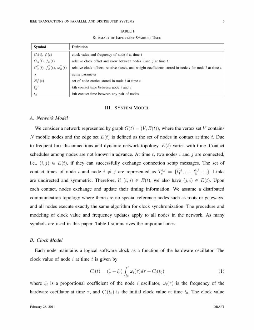
III. SYSTEM MODEL
A. Network Model
We consider a network represented by graph G(t) = (V,E(t)), where the vertex set V contains
N mobile nodes and the edge set E(t) is defined as the set of nodes in contact at time t. Due
to frequent link disconnections and dynamic network topology, E(t) varies with time. Contact
schedules among nodes are not known in advance. At time t, two nodes i and j are connected,
i.e., (i, j) ∈ E(t), if they can successfully exchange connection setup messages. The set of
contact times of node i and node i 6= j are represented as T i,jc = {ti,j1 , . . . , ti,jk , . . .}. Links
are undirected and symmetric. Therefore, if (i, j) ∈ E(t), we also have (j, i) ∈ E(t). Upon
each contact, nodes exchange and update their timing information. We assume a distributed
communication topology where there are no special reference nodes such as roots or gateways,
and all nodes execute exactly the same algorithm for clock synchronization. The procedure and
modeling of clock value and frequency updates apply to all nodes in the network. As many
symbols are used in this paper, Table I summarizes the important ones.
B. Clock Model
Each node maintains a logical software clock as a function of the hardware oscillator. The
clock value of node i at time t is given by
Ci(t) = (1 + ξi)∫ t
t0ωi(τ)dτ + Ci(t0) (1)
where ξi is a proportional coefficient of the node i oscillator, ωi(τ) is the frequency of the
hardware oscillator at time τ , and Ci(t0) is the initial clock value at time t0. The clock value
February 28, 2011 DRAFT
IEEE TRANSACTIONS ON PARALLEL AND DISTRIBUTED SYSTEMS 6
fast clock
Ci’(t)> 1
slow clock
Ci’(t)< 1
perfect clock
Ci’(t)= 1
clock value, Ci(t)
time (t)
(a)
offset
synchronizing
clock
perfect
clock
clock value, Ci(t)
time (t)
Ci’(t)> 1
t1 t2 t3
(b)
synchronizing
clock
clock value, Ci(t)
time (t)
skew
time unit
Ci’(t)= 1
t4
Ci’(t)> 1 perfect
clock
(c)
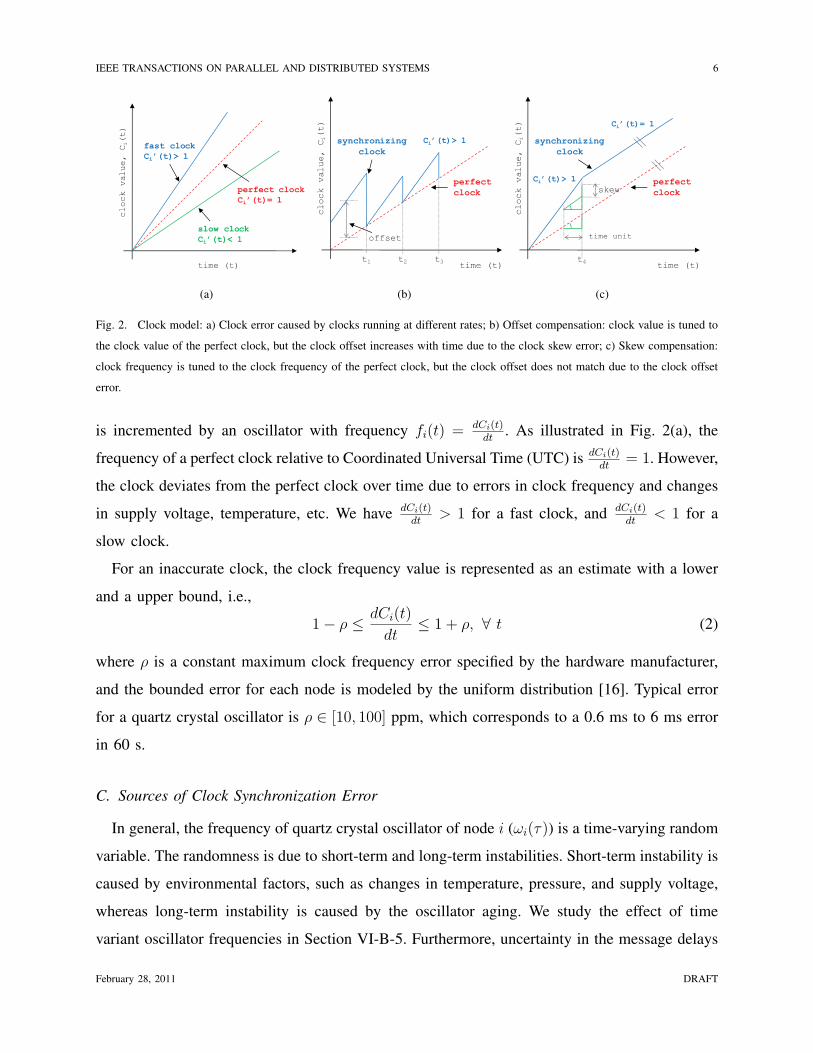
Fig. 2. Clock model: a) Clock error caused by clocks running at different rates; b) Offset compensation: clock value is tuned to
the clock value of the perfect clock, but the clock offset increases with time due to the clock skew error; c) Skew compensation:
clock frequency is tuned to the clock frequency of the perfect clock, but the clock offset does not match due to the clock offset
error.
is incremented by an oscillator with frequency fi(t) = dCi(t)dt
. As illustrated in Fig. 2(a), the
frequency of a perfect clock relative to Coordinated Universal Time (UTC) is dCi(t)dt
= 1. However,
the clock deviates from the perfect clock over time due to errors in clock frequency and changes
in supply voltage, temperature, etc. We have dCi(t)dt
> 1 for a fast clock, and dCi(t)dt
< 1 for a
slow clock.
For an inaccurate clock, the clock frequency value is represented as an estimate with a lower
and a upper bound, i.e.,
1− ρ ≤ dCi(t)
dt≤ 1 + ρ, ∀ t (2)
where ρ is a constant maximum clock frequency error specified by the hardware manufacturer,
and the bounded error for each node is modeled by the uniform distribution [16]. Typical error
for a quartz crystal oscillator is ρ ∈ [10, 100] ppm, which corresponds to a 0.6 ms to 6 ms error
in 60 s.
C. Sources of Clock Synchronization Error
In general, the frequency of quartz crystal oscillator of node i (ωi(τ)) is a time-varying random
variable. The randomness is due to short-term and long-term instabilities. Short-term instability is
caused by environmental factors, such as changes in temperature, pressure, and supply voltage,
whereas long-term instability is caused by the oscillator aging. We study the effect of time
variant oscillator frequencies in Section VI-B-5. Furthermore, uncertainty in the message delays
February 28, 2011 DRAFT
IEEE TRANSACTIONS ON PARALLEL AND DISTRIBUTED SYSTEMS 7
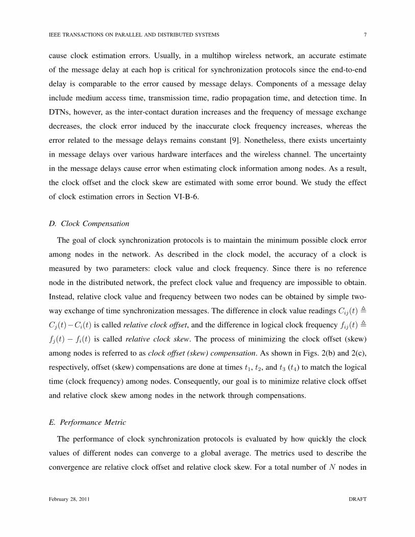
cause clock estimation errors. Usually, in a multihop wireless network, an accurate estimate
of the message delay at each hop is critical for synchronization protocols since the end-to-end
delay is comparable to the error caused by message delays. Components of a message delay
include medium access time, transmission time, radio propagation time, and detection time. In
DTNs, however, as the inter-contact duration increases and the frequency of message exchange
decreases, the clock error induced by the inaccurate clock frequency increases, whereas the
error related to the message delays remains constant [9]. Nonetheless, there exists uncertainty
in message delays over various hardware interfaces and the wireless channel. The uncertainty
in the message delays cause error when estimating clock information among nodes. As a result,
the clock offset and the clock skew are estimated with some error bound. We study the effect
of clock estimation errors in Section VI-B-6.
D. Clock Compensation
The goal of clock synchronization protocols is to maintain the minimum possible clock error
among nodes in the network. As described in the clock model, the accuracy of a clock is
measured by two parameters: clock value and clock frequency. Since there is no reference
node in the distributed network, the prefect clock value and frequency are impossible to obtain.
Instead, relative clock value and frequency between two nodes can be obtained by simple two-
way exchange of time synchronization messages. The difference in clock value readings Cij(t) ,Cj(t)−Ci(t) is called relative clock offset, and the difference in logical clock frequency fij(t) ,fj(t) − fi(t) is called relative clock skew. The process of minimizing the clock offset (skew)
among nodes is referred to as clock offset (skew) compensation. As shown in Figs. 2(b) and 2(c),
respectively, offset (skew) compensations are done at times t1, t2, and t3 (t4) to match the logical
time (clock frequency) among nodes. Consequently, our goal is to minimize relative clock offset
and relative clock skew among nodes in the network through compensations.
E. Performance Metric
The performance of clock synchronization protocols is evaluated by how quickly the clock
values of different nodes can converge to a global average. The metrics used to describe the
convergence are relative clock offset and relative clock skew. For a total number of N nodes in
February 28, 2011 DRAFT

IEEE TRANSACTIONS ON PARALLEL AND DISTRIBUTED SYSTEMS 8
the network, the average relative clock offset and the average relative clock skew at time t are
calculated by
Cavg(t) =1
N(N − 1)/2
N−1∑
i=1
N∑
j=i+1
|Ci(t)− Cj(t)| (3)
favg(t) =1
N(N − 1)/2
N−1∑
i=1
N∑
j=i+1
|fi(t)− fj(t)| . (4)
IV. DISTRIBUTED ASYNCHRONOUS CLOCK SYNCHRONIZATION PROTOCOL
In this section, we propose a distributed asynchronous clock synchronization protocol for
DTNs, which provides global clock synchronization with a distributed algorithm. The DCS
protocol is designed for DTNs where finding or electing reference nodes is difficult and where
connections are often delayed and disrupted among nodes due to mobility and a sparse node
density.
The basic idea of the protocol is to utilize the relative clock information spread in the network
to update clock values, rather than diffusing the information obtained from local neighbors in hop-
by-hop fashion as in existing distributed clock synchronization protocols for multihop wireless
networks. Each node independently manages a table that contains relative clock information.
Upon each new contact, this information is exchanged with the contacted node and transformed
to the compensated logical clock values. Each node uses the clock information in the table to
asynchronously calculate the clock frequency and value that gradually approach their global
averages. To account for a decrease in the accuracy of the propagated clock information, the
contributing weights of the stored information used for the clock compensations are depreciated
over time.
A. Clock Table Structure
We first introduce a structure of the clock table that contains the relative clock information.
At time t, each node i contains a list of other nodes (∀ l ∈ V, l 6= i) in the network that it has
contacted or obtained from contacted nodes. Each node entry in the list is identified by a unique
identifier with following fields: relative clock offset (CTil (t)), relative clock skew (fT
il (t)), and
weight (wTil (t)) which represents the level of information accuracy of node l at node i. Initially,
node i contains only its own information in the list as CTii (0), fT
ii (0) = 0, and wTii(0) = 1. The
set of node entries in the table of node i (NTi (t)) increases when the node obtains information
February 28, 2011 DRAFT

IEEE TRANSACTIONS ON PARALLEL AND DISTRIBUTED SYSTEMS 9
Cj(tj1)
Cj(tj2)
Cj(tj3)
...
Ci(ti1)Ci(t
i1)Ci(t
i2)Ci(t
i2)Ci(t
i3)Ci(t
i3)
Node j
Node i
Cij
time (ti)
time (tj)
(a)
Ci(ti1)
Ci(ti1)
Ci(ti2)
Ci(ti2)
Ci(ti3)
Ci(ti3)
Cj(tj1) Cj(t
j2) Cj(t
j3)
Cij
fij
(b)
Fig. 3. Relative clock estimation: a) Exchanging time-stamps between node i and node j; b) Plotting time-stamped triples for
clock skew estimation.
of a new node. Note that the table entries may become outdated with time and do not represent
the up-to-date differences of the clock values and clock frequencies, i.e., it is possible that
CTil (t) 6= Cil(t) and fT
il (t) 6= fil(t).
A large clock table size may degrade the performance of the network having limited resources
(such as wireless sensor networks) and limited contact durations (such as vehicular networks). In
such scenarios, the clock table overhead can be reduced by various table management techniques.
For example, nodes can decide to store, compute, or exchange a certain maximum number of
entries based on the performance requirement. A higher priority can be given to entries with
higher weights.
B. Exchanging Clock Table Information
In the absence of a reference clock, although the actual clock frequencies fi(ti,jk ) and fj(t
i,jk ) are
impossible to obtain, a relative clock skew (fij(ti,jk )) can be estimated. When node i contacts node
j at time ti,jk , i.e, (i, j) ∈ E(ti,jk ), they exchange series time-stamped triples (Ci(tim), Cj(t
jm), Ci(tim))
for m = 1, 2, . . ., as illustrated in Fig. 3. Here, Ci(tim) is the local time of node i when mth
message is sent, Cj(tjm) is the local time of node j when the mth message is received, and
Ci(tim) is the local time of node i when the reply for the mth message is received from node
j. Then, by plotting series of time-stamped triples, as shown in Fig. 3(b), Cij(ti,jk ) and fij(t
i,jk )
can be estimated by the following linear equation
Ci(tim) = fij(t
i,jk )Cj(t
jm)− Cij(t
i,jk ) (5)
February 28, 2011 DRAFT

IEEE TRANSACTIONS ON PARALLEL AND DISTRIBUTED SYSTEMS 10
representing a line that passes through the bounded errors Ci(tim) and Ci(tim) [22]. More times-
tamps generate tighter estimation error bounds for the relative clock offset and the relative clock
skew.
The update procedure is executed for both nodes i and j upon contact. Without loss of
generality, we present the update procedure for node i here. Since the information of relative
clock offset and relative clock skew between nodes i and j is newly obtained upon the contact,
we update CTij(t
i,jk ) ← Cij(t
i,jk ) and fT
ij (ti,jk ) ← fij(t
i,jk ) for node i. Also, the associated weight
values are reset as wTij(t
i,jk ) = 1. Then, the clock information is updated in the table of node i
for node l 6= i, j if the information about node l received from the node j is more accurate, i.e.,
wTil (t
i,jk ) ≤ wT
jl(ti,jk ). For node i, the updated table information after the exchange is
CTil (t
i,jk ) ←
CTil (t
i,jk ), if wT
il (ti,jk ) ≥ wT
jl(ti,jk )
Cij(ti,jk ) + CT
jl(ti,jk ), otherwise
(6)
fTil (t
i,jk ) ←
fTil (t
i,jk ), if wT
il (ti,jk ) ≥ wT
jl(ti,jk )
fij(ti,jk ) + fT
jl (ti,jk ), otherwise
(7)
wTil (t
i,jk ) ←
wTil (t
i,jk ), if wT
il (ti,jk ) ≥ wT
jl(ti,jk )
wTjl(t
i,jk ), otherwise.
(8)
C. Clock Compensation
In DTNs, skew compensations are equally important as offset compensations. Since offset
compensations cannot be done frequently in the network, even if two nodes start with the same
time value, difference in their logical clock frequencies can result in a large clock offset over
time. For instance, assuming that they have a relative clock skew of just 10 ppm, their time
difference will be 0.6 ms after 60 s, and will further diverge to 36.0 ms after one hour.
Therefore, nodes i and j compensate for offset and skew errors using the updated table infor-
mation. For node i, the compensated clock value and frequency are calculated using weighted
averages as
Ci(ti,jk ) ← Ci(t
i,jk ) +
∑l∈NT
i (ti,jk
)wT
il(ti,jk
)CTil (t
i,jk
)
∑l∈NT
i (ti,jk
)wT
il(ti,j
k)
, fi(ti,jk ) ← fi(t
i,jk ) +
∑l∈NT
i (ti,jk
)wT
il(ti,jk
)fTil (ti,j
k)
∑l∈NT
i (ti,jk
)wT
il(ti,j
k)
(9)
February 28, 2011 DRAFT

IEEE TRANSACTIONS ON PARALLEL AND DISTRIBUTED SYSTEMS 11
and the clock offsets and skews in the table entries, except for CTii (t
i,jk ) and fT
ii (ti,jk ), are updated
as
CTil (t
i,jk ) ← CT
il (ti,jk )−
∑l∈NT
i (ti,jk
)wT
il(ti,jk
)CTil (t
i,jk
)
∑l∈NT
i (ti,jk
)wT
il(ti,j
k)
, fTil (t
i,jk ) ← fT
il (ti,jk )−
∑l∈NT
i (ti,jk
)wT
il(ti,jk
)fTil (ti,j
k)
∑l∈NT
i (ti,jk
)wT
il(ti,j
k)
.
(10)
Note that, since wTii represents the level of accuracy of its own clock information, wT
ii is always
one. Therefore, (9) includes the case for l = i to account for wTii . Also, by definition, since the
relative clock offset and skew of a node to itself are both zero, CTii and fT
ii are initially assigned
zero (see section IV-A) and remain unchanged.
While the updated values of offsets and skews do not change between contacts, the contributing
weights in the table of node i are decreased between contacts to account for the decrease of the
accuracy of clock information with time. Suppose two consecutive contacts of node i take place
at times t and t + ∆t, we have
wTil (t + ∆t) =
1, if l = i
wTil (t)λ
∆t, otherwise(11)
where λ ∈ [0, 1] is the aging parameter and ∆t is the time elapsed in seconds between two con-
secutive contacts. Note that λ = 1 corresponds to propagating information without depreciating
the weight over time, while λ = 0 corresponds to only making use of the information about the
contacted node. The contact time for each node is unknown in advance, but the time difference
between two contact times can be calculated upon each new contact. Although, the calculation
of ∆t may not be accurate due to clock errors of node itself, since the inter-contact durations in
the DTNs are usually much larger than the error, the effect of the estimation error is negligible.
Note that a backward clock movement is not acceptable for some applications. Whereas the
logical clock frequency can be changed immediately by applying the skew compensation, the
time of a clock cannot run backward by applying a negative offset compensation. A common
solution to this problem is to freeze the time of the node until the other node, having a slower
time and applied with a positive offset compensation, reaches the same time [19]. This solution
can be considered in implementing the DCS protocol to solve the backward clock movement
problem.
February 28, 2011 DRAFT

IEEE TRANSACTIONS ON PARALLEL AND DISTRIBUTED SYSTEMS 12
D. Convergence Analysis
In this section, we show that the clocks running the DCS protocol converge to a common
value. For the analysis, the identities of all N nodes in the network are assumed to be known.
Let the set of contact times between any pair of nodes in the network be defined as Tc =⋃
i,j∈V T i,jc = {t1, . . . , tk, . . .}. Since fi(tk) is constant between contacts for all i ∈ V and Ci(tk)
is dependent on fi(tk), if fi(tk) converges to a common value, the convergence of Ci(tk) simply
follows the convergence proof of fi(tk). Therefore, we focus on the convergence proof of the
clock frequency, fi(tk).
The clocks in the network converge if the relative clock skews converge to zero as
limtk→∞
maxi,j∈V
|fij(tk)| = 0. (12)
or equivalently, for some constant value fs, if
limtk→∞
maxj∈V
fj(tk) = limtk→∞
mini∈V
fi(tk) = fs. (13)
The convergence proof can be simplified by the following lemma.
Lemma 1. With the DCS protocol, the resulting frequencies of node i, after the updates using
relative skews in the table (fTil (tk)) and the outdated actual frequencies (fl(t
dil(tk))), are the
same, where 0 ≤ tdil(tk) represents the time when the frequency value of node l was recorded
and observed by node i at time tk, as illustrated in Fig. 4.
Proof: According to (9), when node i contacts with node j, the update using the relative
clock skews with respect to the underlying actual clock frequency can be calculated as
fi(tk) +
∑Nl=1 wT
il (tk)fTil (tk)∑N
l=1 wTil (tk)
= fi(tk) +
∑Nl=1 wT
il (tk)(fl(tdil(tk))− fi(tk))∑N
l=1 wTil (tk)
= fi(tk) +
∑Nl=1 wT
il (tk)fl(tdil(tk))∑N
l=1 wTil (tk)
−∑N
l=1 wTil (tk)fi(tk)∑N
l=1 wTil (tk)︸ ︷︷ ︸
fi(tk)
=
∑Nl=1 wT
il (tk)fl(tdil(tk))∑N
l=1 wTil (tk)
. (14)
Note that we have fTil (tk) = fl(t
dil(tk))−fi(tk) in (14) since the clock compensation is performed
for both clock frequency fi(ti,jk ) in (9) and clock skews fT
il (ti,jk ) in (10), which preserves the
recorded actual clock frequency fl(tdil(tk)) upon each contact.
February 28, 2011 DRAFT

IEEE TRANSACTIONS ON PARALLEL AND DISTRIBUTED SYSTEMS 13
tdBC(t2)=tdAC(t2)
=tdAC(t1)=t1
t1 time (t)t2
tdAC(t1)=t1
(a) (A,C) E(t1) (b) (A,B) E(t2)
Fig. 4. An illustrative example of delayed information: (a) At time t1, nodes A and C contact with each other, and node A
obtains the clock frequency value of node C (fC(t1)) directly from node C; (b) At time t2, nodes A and B contact with each
other, and the clock frequency value of node C (fC(tdBC(t2))) is forwarded to node B via node A.
Let F (tk) = [f1(tk); . . . ; fN(tk)]T represent the N state vector containing the clock frequencies
at time tk. Based on Lemma 1, the update procedure of the DCS protocol can be formulated as
an consensus/agreement problem [23], where the updated frequencies after the kth update can
be calculated as
fi(tk) =N∑
l=1
ail(tk)fl(tdil(tk)),∀ i ∈ V. (15)
Define A(tk) as an N ×N matrix containing normalized weights ail(tk) ∈ [0, 1], which is given
by
ail(tk) =
wTil (tk)/(
∑Nn=1 wT
il (tk)), if ∃ j 6= i, (i, j) ∈ E(tk)
I(l = i), otherwise(16)
where wTil (tk) is the decaying weight defined in (11) and I(·) is an indication function which
equals 1 if true and 0 otherwise. In (16), the first case corresponds to node i contacts with
another node, while the second case occurs when there is no contact between node i and any
other node, and thus there is no update for clock frequency of node i. Moreover, in (15), we
have tdii(tk) = tk since each node can acquire the clock information of itself without delay.
Theorem 1. (Convergence of the DCS protocol) The clock values using the DCS protocol
converge to a common value under deterministic mobility scenarios, and converges to the value
with probability under random mobility scenarios.
Proof: Based on the consensus theorem [24, 25], if the following conditions are satisfied,
((1) the update weight matrices are row stochastic, (2) the network is strongly connected, and (3)
the communication delay is bounded such that tk − B < tdil(tk) ≤ tk) the algorithm guarantees
asymptotic consensus: Condition (1) is satisfied for the DCS since it can be easily verified
February 28, 2011 DRAFT
IEEE TRANSACTIONS ON PARALLEL AND DISTRIBUTED SYSTEMS 14
that A(tk) ∈ <N×N and A(tk)1N = 1N ∀ tk, where 1N = [1; . . . ; 1]T . Conditions (2) and (3)
are satisfied depending on the mobility scenarios. The connectivity graph is strongly connected
if there is a path from each vertex in the graph to every other vertex. In mobile networks,
a virtual path exists from a source node to a destination node if messages can be forwarded
using one or more mobile nodes acting as intermediate nodes, and the communication delay
is the sum of inter-contact durations from the source node to the destination node. Thus, the
network is strongly connected if there exists a forwarding path from each node in the graph
to every other node, i.e., there is no isolated node. The delay is bounded (tk − tdil(tk) < B),
if the sum of the inter-contact durations over the forwarding path is bounded. Specifically, in
deterministic mobility scenarios, such as bus routes [8] and message ferries [26, 27], where the
mobility is planned or controlled such that the forwarding paths are consistently available and
nodes contact following certain schedule, the clock values asymptotically converges. On the other
hand, in random mobility scenarios, such as random waypoint (RWP) and random direction (RD),
the inter-contact duration is modeled by a probability distribution. As a result, the inter-contact
duration is bounded with certain probability. Since an unbounded inter-contact duration leads
to an unbounded delay, the DCS protocol converges with probability [28] in random mobility
scenarios.
As the probability for the delay to exceed a bound B is low when B is large according to the
analysis [29, 30], the probability for the DCS protocol to converge is high for most scenarios.
Note that considering N instead of NTi (t) in the analysis does not change the convergence result
since the weight values, except for i = j, are all initialized to zero and they do not contribute
to the updates as if their identities are unknown.
Based on the convergence proof of the DCS protocol, the convergence of the AD protocol
can be also proved. The AD protocol is a special case of the DCS protocol having tdij(tk) =
tdji(tk) = tk and ail(tk) given by
ail(tk) =
1/2, if ∃ j 6= i, (i, j) ∈ E(tk) and l = i, j
I(l = i), otherwise.(17)
Different convergence proofs for the AD protocol can be found in [17, 20, 24, 31].
Furthermore, since the information stored in the tables becomes less accurate with time and
different table entries have different accuracy, a weighting mechanism with a tunable aging
February 28, 2011 DRAFT

IEEE TRANSACTIONS ON PARALLEL AND DISTRIBUTED SYSTEMS 15
parameter (λ) in (11) is adopted in the DCS protocol to better utilize the table entries with higher
accuracy. The effect of λ on the convergence speed will be shown by analysis and simulation
in Subsection VI-A and Subsection VI-B, respectively.
V. PERFORMANCE ANALYSIS
In this section, a discrete time analysis is proposed to evaluate the performance of the DCS
protocol. Different from the convergence analysis in Subsection IV-D, we consider a fixed time
interval (τ ) in this section since the analytical complexity is prohibitive to keep all contact
histories. For analytical tractability, the following assumptions are made:
1) The movement of all mobile nodes are independent and the pairwise inter-contact duration
is approximately exponentially distributed with an average value 1/γ;
2) The density of mobile nodes is low and the probability for more than two mobile nodes
to contact with each other simultaneously is negligible.
The assumption 1) holds for numerous random mobility models, such as in random waypoint
(RWP) and random direction (RD) [29, 30, 32, 33], and real mobility traces [34, 35]. The
performance analysis of the DCS protocol consists of two parts. In Subsection V-A, the table
updating procedure is modeled. In Subsection V-B, the performance metrics in terms of the
average relative clock offset and the average relative clock skew are evaluated by considering
the updated table information.
A. Modeling of Table Updating Procedure
For analytical simplicity, we consider the clock value and clock frequency as the table entries
for the DCS protocol, which are equivalent to the clock offset and clock skew since the accurate
clock information of each node is available in the analytical model. Denote Xil(τk) and Yil(τk)
as the clock value and clock frequency, respectively, of node l recorded in the table of node i
at time τk = kτ (k = 0, 1, 2, · · · ), which are given by
Xii(τk) = Ci(τk), Yii(τk) = fi(τk) (18)
Xil(τk) = CTil (τk) + Ci(τk), Yil(τk) = fT
il (τk) + fi(τk), i 6= l. (19)
Note that Xil(τk) and Yil(τk) may not have the same values as Xll(τk) and Yll(τk) since the table
entries CTil (τk) and fT
il (τk) may be outdated.
February 28, 2011 DRAFT

IEEE TRANSACTIONS ON PARALLEL AND DISTRIBUTED SYSTEMS 16
1) Table Updating Procedure of the Clock Frequency: The clock frequency Yil(τk) of node
l stored in the table of node i can be updated by (1) a direct contact with node l and (2) an
indirect contact through some nodes other than l, or (3) remain unchanged without any contact.
First, Yil(τk) can be updated by a direct contact with node l. Since the historic contact
information is not available in the discrete time model, the approximated contributing weight is
used for analytical tractability. The updated clock frequency of node i when it contacts node l
within τ is given by
Yil(τk+1) =
∑Nh=1 wT
(n∗ilh
(τk+1))h(τk+1)Y(n∗
ilh(τk+1))h(τk)
∑Nh=1 wT
(n∗ilh
(τk+1))h(τk+1)
(20)
where wTnh(τk+1) is the approximated contributing weight with respect to node h in the table
of node n and n∗ilh(τk+1) denotes the node (either node i or node l) with a higher contributing
weight with respect to node h (h = 1, · · · , N ). Here, the value of wTnh(τk+1) is estimated based
on the instantaneous clock value and clock frequency as follows
wTnh(τk+1) =
1, if h = i or l
λTnh(τk+1), otherwise(21)
where Tnh(τk+1) is the approximated elapsed time since the clock information of node h was
recorded. The value of Tnh(τk+1) can be calculated based on the difference between the clock
value divided by the difference between the clock frequency, and is given by
Tnh(τk+1) =
∣∣∣ [Xhh(τk)+τYhh(τk)]−[Xnh(τk)+τYnn(τk)]Yhh(τk)−Ynn(τk)
∣∣∣ , if Yhh(τk) 6= Ynn(τk)
∞, otherwise.(22)
Also, the value of n∗ilh(τk+1) is determined based on the accuracy of the table entry as follows
n∗ilh(τk+1) = arg minn∈{i,l}
|[Xnh(τk) + τYnn(τk)]− [Xhh(τk+1) + τYhh(τk)]| (23)
where the terms τYnn(τk) and τYhh(τk) are applied since the clock value of each node changes
at a constant rate according to the clock frequency if there is no contact with other nodes during
τ . Note that the table entries of clock values are updated according to the clock frequency of
the node keeping the table.
Second, Yil(τk) can be updated by an indirect contact with some nodes other than l that has
the clock frequency of node l in its table. The updated clock frequency in the table of node i
February 28, 2011 DRAFT

IEEE TRANSACTIONS ON PARALLEL AND DISTRIBUTED SYSTEMS 17
with respect to node l, when node i contacts with node j (j 6= i, l) within τ , is given by
Yijl(τk+1) = Y(n∗ijl
(τk+1))l(τk). (24)
Third, Yil(τk) remains unchanged if there is no contact between node i and any of the other
(N − 1) nodes within τ .
Finally, the table updating procedure of the clock frequencies in the DCS protocol considering
all three cases can be modeled as
Yil(τk+1) =1− P0
(N − 1)Yil(τk+1) +
N∑
j=1j 6=i,l
1− P0
(N − 1)Yijl(τk+1) + P0Yil(τk), i 6= l (25)
where P0 = (e−γτ )N−1 is the probability that there is no contact between node i and any of the
other (N − 1) nodes within τ . An approximation is made in the analysis that the probability for
more than one contact between node i and any of the other (N−1) nodes within τ is negligible.
Since node i contacts with any of the other (N − 1) nodes with the same probability, the factor1
(N−1)is applied.
2) Table Updating Procedure of the Clock Value: The clock value Xil(τk) of node l stored
in the table of node i is updated also for the same three cases used in the modeling of the table
updating procedure of the clock frequency. However, different from the table updating procedure
of the clock frequency, the table entries of clock values change not only when two nodes contact
with each other, but also over time according to the clock frequency.
First, the updated clock value of node i when it contacts node l within τ is given by
Xil(τk+1) =
∑Nh=1 wT
(n∗ilh
(τk+1))h(τk+1)[X(n∗
ilh(τk+1))h(τk) + τY(n∗
ilh(τk+1))(n
∗ilh
(τk+1))(τk)]∑N
h=1 wT(n∗
ilh(τk+1))h
(τk+1)(26)
where the term τY(n∗ilh
(τk+1))(n∗ilh
(τk+1))(τk) is applied to the numerator since the clock value
changes according to the clock frequency during τ .
Second, the updated clock value in the table of node i with respect to node l, when node i
contacts with node j (j 6= i, l) within τ , is given by
Xijl(τk+1) = X(n∗ijl
(τk+1))l(τk) + τY(n∗ijl
(τk+1))(n∗ijl
(τk+1))(τk). (27)
Third, the clock value of node l stored in node i when there is no contact between node i
and any of the other (N − 1) nodes within τ is given by Xil(τk) + τYii(τk).
February 28, 2011 DRAFT
IEEE TRANSACTIONS ON PARALLEL AND DISTRIBUTED SYSTEMS 18
Finally, the table updating procedure of the clock values in the DCS protocol can be modeled
as
Xil(τk+1) =1− P0
(N − 1)Xil(τk+1) +
N∑
j=1j 6=i,l
1− P0
(N − 1)Xijl(τk+1) + P0 [Xil(τk) + τYii(τk)] , i 6= l. (28)
B. Evaluation of Performance Metrics
Based on the modeling of the table updating procedure, the update of the clock value and
clock frequency are given by
Xii(τk+1) =N∑
l=1l 6=i
1− P0
(N − 1)Xil(τk+1) + P0 [Xii(τk) + τYii(τk)] (29)
Yii(τk+1) =N∑
l=1l 6=i
1− P0
(N − 1)Yil(τk+1) + P0Yii(τk) (30)
where Xil(τk+1) and Yil(τk+1) are given by (26) and (20), respectively.
Define the system state of the DCS protocol at time τk as SDCS(τk) = {Xil(τk), Yil(τk)|i, l =
1, · · · , N}. For the updating procedure in (25), and (28)-(30), only the current system state
SDCS(τk) is needed to obtain the next system state SDCS(τk+1). Therefore, we can define an
operation FDCS(·) such that SDCS(τk+1) = FDCS(SDCS(τk)). Given the initial clock values
Xii(0) = Ci(0) and clock frequency Yii(0) = fi(0), and the initial values of table entries
Xil(0) = Xii(0) and Yil(0) = Yii(0) (i 6= l), the system state of the DCS protocol at time τk can
be calculated as
SDCS(k) = F kDCS(SDCS(0)) (31)
where F kDCS(·) denotes applying the operation FDCS(·) by k times. Then the performance metrics
at time τk (Cavg(τk) and favg(τk)) of the DCS protocol can be calculated. Based on the analytical
model of the DCS protocol, we can also evaluate the performance of the AD protocol without
considering the table updating procedure. The detailed derivation is presented in Appendix.
VI. PERFORMANCE EVALUATION
In this section, numerical and simulation results are presented to evaluate the performance
of the proposed DCS protocol. The numerical results (Ana.) are based on the analytical model
February 28, 2011 DRAFT

IEEE TRANSACTIONS ON PARALLEL AND DISTRIBUTED SYSTEMS 19
TABLE II
DEFAULT SYSTEM PARAMETER
Parameter Value
Simulation Time 550 hours
Map Size (M ×M ) 50 km × 50 km, 20 km × 20 km
Number of Nodes (N ) 50
Node Speed (v) Uniform(0.5, 1.5) m/s
Pause Time 0 - 120 s
Radio Transmission Range (R) 250 m
Initial Skew (C′i(t0)) Uniform(−100, +100) ppm
Initial Offset (Ci(t0)) Uniform(−106, +106) µs
Aging Constant (λ) 1− 10−5
presented in Section V, while the simulation results are obtained based on a discrete event-
driven simulator using exponentially distributed inter-contact durations (Sim. Exp.) and the
Opportunistic Network Environment (ONE) simulator [36] with an additional implementation of
the clock synchronization mechanism (Sim. RWP). Note that in the analysis, contacts are assumed
to be one-to-one for analytical tractability. However, since both simulators are event-driven, table
updating procedure is performed whenever there is a new connection created between any pair of
nodes, regardless of the number of simultaneous connections. If there are multiple new contacts,
connections are created in the increasing order of the node ID. Still, chances of having multiple
new connections in the same event interval is negligibly small for all nodes. Default system
parameters are given in Table II.
A. Numerical Results
For the RWP mobility model under consideration, the pairwise inter-contact duration is ap-
proximately exponentially distributed [30, 32]. Both theoretical and experimental results can be
used to estimate the pairwise inter-contact rate γ. In this work, γ is estimated as the reciprocal
of the average pairwise inter-contact duration obtained from simulation results. We consider two
network coverage areas. The density of mobile nodes is configured to create a disconnected
network with a node degree much smaller than 1 [37] and hence nodes are mostly disconnected.
The pairwise inter-contact rate for M = 20 km and M = 50 km is 2.15 × 10⁻⁶s−1 and
4.05 × 10⁻⁷s−1, respectively. Since the clock values Xii(τk) and frequencies Yii(τk) of the N
February 28, 2011 DRAFT

IEEE TRANSACTIONS ON PARALLEL AND DISTRIBUTED SYSTEMS 20
0
100000
200000
300000
400000
500000
600000
700000
800000
900000
0 20 40 60 80 100
Rel
ativ
e C
lock
Offs
et (
us)
Time (hour)
AD Ana.AD Sim. Exp. AD Sim. RWPDCS Ana.DCS Sim. Exp.DCS Sim. RWP
(a)
0
10
20
30
40
50
60
70
0 20 40 60 80 100
Rel
ativ
e C
lock
Ske
w (
ppm
)
Time (hour)
AD Ana.AD Sim. Exp. AD Sim. RWPDCS Ana.DCS Sim. Exp.DCS Sim. RWP
(b)
Fig. 5. Convergence of clock offset and skew (M = 20 km): (a) Average relative clock offset; (b) Average relative clock skew.
0
1e+006
2e+006
3e+006
4e+006
5e+006
6e+006
0 100 200 300 400 500 600
Rel
ativ
e C
lock
Offs
et (
us)
Time (hour)
AD Ana.AD Sim. Exp. AD Sim. RWPDCS Ana.DCS Sim. Exp.DCS Sim. RWP
(a)
0
10
20
30
40
50
60
70
0 100 200 300 400 500 600
Rel
ativ
e C
lock
Ske
w (
ppm
)
Time (hour)
AD Ana.AD Sim. Exp. AD Sim. RWPDCS Ana.DCS Sim. Exp.DCS Sim. RWP
(b)
Fig. 6. Convergence of clock offset and skew (M = 50 km): (a) Average relative clock offset; (b) Average relative clock skew.
nodes are updated simultaneously for each time period τ in (29) and (30), we consider τ = N
(N2 )γ
,
where(
N2
)γ equals the average inter-contact rate for all combinations of pairwise contacts. Note
that, during τ , N updates of clock values and frequencies take place on average.
1) Impact of Node Density: Figs. 5 and 6 show the average relative clock offset and skew
for M = 20 km and M = 50 km, respectively. For both node densities, the clock offset
of the DCS protocol converges faster than that of the AD protocol. The divergence in the
beginning is due to large initial relative clock skews that produce large time differences during
long delays between connections. The clock offsets gradually converge to zero as the clock
skews converge exponentially with time as shown in Figs. 5(b) and 6(b). Since nodes have more
contact opportunities among them at higher node densities, the convergence speed is faster and
February 28, 2011 DRAFT

IEEE TRANSACTIONS ON PARALLEL AND DISTRIBUTED SYSTEMS 21
0.01
0.1
1
0 500000 1e+006 1.5e+006 2e+006
Inte
r-C
onta
ct D
urat
ion
(ccd
f)
Time (s)
RWPExponential
(a)
0.01
0.1
1
0 3e+006 6e+006 9e+006 1.2e+007
Inte
r-C
onta
ct D
urat
ion
(ccd
f)
Time (s)
RWPExponential
(b)
Fig. 7. Distribution of inter-contact duration: (a) M = 20 km, γ = 2.15× 10⁻⁶s−1; (b) M = 50 km, γ = 4.05× 10⁻⁷s−1.
the initial divergence of relative clock offset is smaller when M = 20 km.
Overall, for both the AD and DCS protocols, the analytical and simulation results, using
the same average inter-contact durations, match well with each other. The estimation error in
Ana. and Sim. Exp. in comparison with Sim. RWP are caused by the fact that the inter-contact
durations of the RWP mobility model are only approximately exponentially distributed, as shown
in Fig. 7. Similar observations have been obtained for the RD mobility model [32]. In addition,
although, the Ana. result and the Sim. Exp. result of relative clock skew match well with each
other, the Ana. result of relative clock offset is smaller than the Sim. Exp. result. The reason is
that, the table entries in the discrete time analysis of Ana. are updated at the end of each discrete
period (with duration τ ), whereas the table entries in the event-driven simulator Sim. Exp. are
updated at random moments. Consequently, considering the updated entries at the end of each
period with constant clock frequencies, the Ana. result indicates smaller relative clock offset
results by neglecting the divergence of relative clock offset in between the discrete periods.
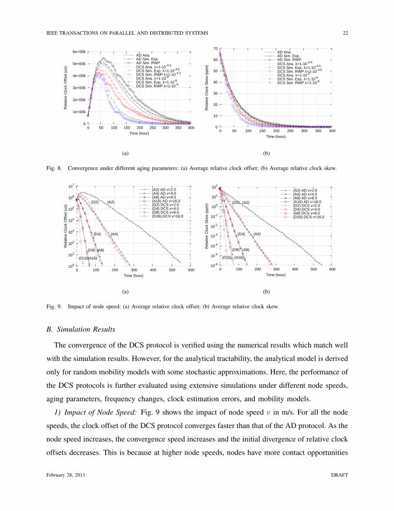
2) Impact of Aging Parameter: Fig. 8 shows the average relative clock offset and skew
for the DCS protocol with respect to time t for various λ values. Although the elapsed time
for the contributing weight calculation is approximated by (22) based on the instantaneous
clock value and clock frequency, the proposed analytical model provides a good estimate of
the two performance metrics for different λ values in all the scenarios. In practical applications,
when the pair-wise inter-contact duration is approximately exponentially distributed, the proposed
analytical model can be used as an efficient tool to facilitate the system performance estimation.
February 28, 2011 DRAFT
IEEE TRANSACTIONS ON PARALLEL AND DISTRIBUTED SYSTEMS 22
0
1e+006
2e+006
3e+006
4e+006
5e+006
6e+006
0 50 100 150 200 250 300 350 400
Rel
ativ
e C
lock
Offs
et (
us)
Time (hour)
AD Ana. AD Sim. Exp.AD Sim. RWPDCS Ana. λ=1-10-4.5
DCS Sim. Exp. λ=1-10-4.5
DCS Sim. RWP λ=1-10-4.5
DCS Ana. λ=1-10-6
DCS Sim. Exp. λ=1-10-6
DCS Sim. RWP λ=1-10-6
(a)
0
10
20
30
40
50
60
70
0 50 100 150 200 250 300 350 400
Rel
ativ
e C
lock
Ske
w (
ppm
)
Time (hour)
AD Ana. AD Sim. Exp.AD Sim. RWPDCS Ana. λ=1-10-4.5
DCS Sim. Exp. λ=1-10-4.5
DCS Sim. RWP λ=1-10-4.5
DCS Ana. λ=1-10-6
DCS Sim. Exp. λ=1-10-6
DCS Sim. RWP λ=1-10-6
(b)
Fig. 8. Convergence under different aging parameters: (a) Average relative clock offset; (b) Average relative clock skew.
100
101
102
103
104
105
106
107
0 100 200 300 400 500 600
Rel
ativ
e C
lock
Offs
et (
us)
Time (hour)
(A2) AD v=2.0(A4) AD v=4.0(A8) AD v=8.0(A16) AD v=16.0(D2) DCS v=2.0(D4) DCS v=4.0(D8) DCS v=8.0(D16) DCS v=16.0
(A2)
(A4)
(A8)
(A16)
(D2)
(D4)
(D8)
(D16)
(a)
10-6
10-5
10-4
10-3
10-2
10-1
100
101
102
0 100 200 300 400 500 600
Rel
ativ
e C
lock
Ske
w (
ppm
)
Time (hour)
(A2) AD v=2.0(A4) AD v=4.0(A8) AD v=8.0(A16) AD v=16.0(D2) DCS v=2.0(D4) DCS v=4.0(A8) DCS v=8.0(D16) DCS v=16.0
(A2)
(A4)
(A8)
(A16)
(D2)
(D4)
(D8)
(D16)
(b)
Fig. 9. Impact of node speed: (a) Average relative clock offset; (b) Average relative clock skew.
B. Simulation Results
The convergence of the DCS protocol is verified using the numerical results which match well
with the simulation results. However, for the analytical tractability, the analytical model is derived
only for random mobility models with some stochastic approximations. Here, the performance of
the DCS protocols is further evaluated using extensive simulations under different node speeds,
aging parameters, frequency changes, clock estimation errors, and mobility models.
1) Impact of Node Speed: Fig. 9 shows the impact of node speed v in m/s. For all the node
speeds, the clock offset of the DCS protocol converges faster than that of the AD protocol. As the
node speed increases, the convergence speed increases and the initial divergence of relative clock
offsets decreases. This is because at higher node speeds, nodes have more contact opportunities
February 28, 2011 DRAFT

IEEE TRANSACTIONS ON PARALLEL AND DISTRIBUTED SYSTEMS 23
100
101
102
103
104
105
106
107
0 100 200 300 400 500 600
Rel
ativ
e C
lock
Offs
et (
us)
Time (hour)
(A1) AD(A2) DCS λ=1-10-3 (A3) DCS λ=1-10-4.5 (A4) DCS λ=1-10-5
(A5) DCS λ=1-10-6
(A1)(A2)
(A3)
(A4)
(A5)
(a)
10-6
10-5
10-4
10-3
10-2
10-1
100
101
102
0 100 200 300 400 500 600
Rel
ativ
e C
lock
Ske
w (
ppm
)
Time (hour)
(A1) AD(A2) DCS λ=1-10-3
(A3) DCS λ=1-10-4.5
(A4) DCS λ=1-10-5
(A5) DCS λ=1-10-6
(A1)(A2)(A3)
(A4)(A5)
(b)
Fig. 10. Impact of aging parameter: (a) Average relative clock offset; (b) Average relative clock skew.
among them.
2) Impact of Aging Parameter: The impact of the tuning parameter λ in (11) is shown in
Fig. 10. For this specific scenario, λ = 1 − 10−6 achieves the lowest relative clock offset until
about 200 h, but at the end of the simulation, the average relative clock offsets of the DCS
protocol with λ = 0 (same as the AD protocol), λ = 1 − 10−3, λ = 1 − 10−4.5, λ = 1 − 10−5,
and λ = 1− 10−6 are 13148 µs, 12632 µs, 4463 µs, 3 µs, and 13 µs, respectively. This result
indicates that there exists some optimal λ value for each scenario. The impact of different
aging parameter values can also be seen in Fig. 10(b) for the skew result. The aging parameter
can be selected to effectively discard the information that becomes less accurate over time. If
some nodes fail or become isolated so that they are unable to propagate their information to
the whole network, the outdated information coupled with long inter-contact delays under the
disconnected network topology can increase the average relative clock values. On the other hand,
when λ = 1−10−3, the DCS protocol operates similarly to the AD protocol since wTij(t) quickly
approaches zero, and by the time a new contact is discovered, CTij(t) and fT
ij (t) have a negligible
share in the compensation algorithm. However, how to analytically acquire the optimal values
of λ for different scenarios is still an open problem.
3) Impact on Energy Consumption: In order to demonstrate the impact of synchronization
error on energy consumption, simulation result for the average energy consumption in neighbor
discovery is shown in Fig. 11. Each node uses a sleep schedule with a duty cycle TD and
awake periods with lengths 2Cmax(t) + TA ≤ TD where Cmax(t) = max |Cij(t)| ,∀ i, j, is the
February 28, 2011 DRAFT
IEEE TRANSACTIONS ON PARALLEL AND DISTRIBUTED SYSTEMS 24
10-5
10-4
10-3
10-2
10-1
100
101
0 100 200 300 400 500 600
Pow
er C
onsu
mpt
ion
(W)
Time (hour)
(A20) AD (TD=20 s)(A5) AD (TD=5 s)(D20) DCS (TD=20 s)(D5) DCS (TD=5 s)(P20) Perfect (TD=20 s)(P5) Perfect (TD=5 s)
(A5)
(A20)(D5)
(D20)
(P5)
(P20)
(a)
0
5000
10000
15000
20000
25000
30000
35000
40000
45000
0 100 200 300 400 500 600
Ene
rgy
Con
sum
ptio
n (J
)
Time (hour)
(A20) AD (TD=20 s)(A5) AD (TD=5 s)(D20) DCS (TD=20 s)(D5) DCS (TD=5 s)(P20) Perfect (TD=20 s)(P5) Perfect (TD=5 s)
(A20)
(A5)
(D20)
(D5)
(P20)(P5)
(b)
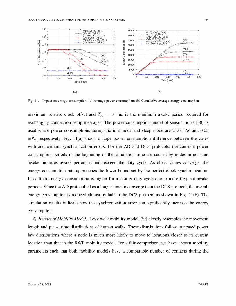
Fig. 11. Impact on energy consumption: (a) Average power consumption; (b) Cumulative average energy consumption.
maximum relative clock offset and TA = 10 ms is the minimum awake period required for
exchanging connection setup messages. The power consumption model of sensor motes [38] is
used where power consumptions during the idle mode and sleep mode are 24.0 mW and 0.03
mW, respectively. Fig. 11(a) shows a large power consumption difference between the cases
with and without synchronization errors. For the AD and DCS protocols, the constant power
consumption periods in the beginning of the simulation time are caused by nodes in constant
awake mode as awake periods cannot exceed the duty cycle. As clock values converge, the
energy consumption rate approaches the lower bound set by the perfect clock synchronization.
In addition, energy consumption is higher for a shorter duty cycle due to more frequent awake
periods. Since the AD protocol takes a longer time to converge than the DCS protocol, the overall
energy consumption is reduced almost by half in the DCS protocol as shown in Fig. 11(b). The
simulation results indicate how the synchronization error can significantly increase the energy
consumption.
4) Impact of Mobility Model: Levy walk mobility model [39] closely resembles the movement
length and pause time distributions of human walks. These distributions follow truncated power
law distributions where a node is much more likely to move to locations closer to its current
location than that in the RWP mobility model. For a fair comparison, we have chosen mobility
parameters such that both mobility models have a comparable number of contacts during the
February 28, 2011 DRAFT

IEEE TRANSACTIONS ON PARALLEL AND DISTRIBUTED SYSTEMS 25
102
103
104
105
106
0 4000 8000 12000 16000 20000
Rel
ativ
e C
lock
Offs
et (
us)
Time (s)
(AR) AD RWP(AL) AD Levy walk(DR) DCS RWP(DL) DCS Levy walk
(AR)
(AL)
(DR)
(DL)
(a)
10-2
10-1
100
101
102
0 4000 8000 12000 16000 20000
Rel
ativ
e C
lock
Ske
w (
ppm
)
Time (s)
(AR) AD RWP(AL) AD Levy walk(DR) DCS RWP(DL) DCS Levy walk
(AR)
(AL)
(DR)
(DL)
(b)
Fig. 12. Impact of mobility model (M = 5 km): (a) Average relative clock offset; (b) Average relative clock skew.
0 0.1 0.2 0.3 0.4 0.5 0.6 0.7 0.8 0.9
1
0 4000 8000 12000 16000 20000
Inte
r-C
onta
ct D
urat
ion
(CD
F)
Time (s)
RWPLevy walk
Fig. 13. Distribution of inter-contact duration (M = 5 km)
simulations1. The average number of contacts during the simulations for RWP and Levy walk
mobility model are 1680 and 1682, respectively. Fig. 12(a) shows that the clock offset converges
faster for RWP. Even though the total number of contacts is slightly higher for the Levy walk
mobility, nodes for Levy walk have a higher probability to contact with the nodes that are closer
to their current location (i.e., node mobility is less diffusive), as shown in Fig. 13. Therefore,
the convergence speed depends on how evenly the probability of meeting different nodes is
distributed.
5) Impact of Clock Frequency Instability: We investigate the impact of the clock frequency
instabilities on the clock convergence. First, the impact of short-term clock frequency instability
1Exact parameters used to generate the traces of Levy walk mobility patterns are as follows: power-law slope of flight length
α = 0.4, power-law slot of pause time β = 0.5, scale factor of flight length = 2.5, truncated flight length = 3000 m, and
truncated pause time = 120 s. Please refer to [39] for the detailed description of the model and the choice of the parameters
used in the trace generation.
February 28, 2011 DRAFT
IEEE TRANSACTIONS ON PARALLEL AND DISTRIBUTED SYSTEMS 26
100
101
102
103
104
105
106
107
0 100 200 300 400 500 600
Rel
ativ
e C
lock
Offs
et (
us)
Time (hour)
(A1) AD(D1) DCS
(A1)
(D1)
(a)
10-6
10-5
10-4
10-3
10-2
10-1
100
101
102
0 100 200 300 400 500 600
Rel
ativ
e C
lock
Ske
w (
ppm
)
Time (hour)
(A1) AD(D1) DCS
(A1)
(D1)
(b)
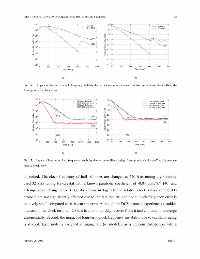
Fig. 14. Impact of short-term clock frequency stability due to a temperature change: (a) Average relative clock offset; (b)
Average relative clock skew.
100
101
102
103
104
105
106
107
0 200 400 600 800 1000 1200 1400
Rel
ativ
e C
lock
Offs
et (
us)
Time (hour)
(A5) AD d=5 ppm(D5) DCS d=5 ppm(A0) AD d=0 ppm(D0) DCS d=0 ppm
(A5)
(D5)
(A0)
(D0)
(a)
10-6
10-5
10-4
10-3
10-2
10-1
100
101
102
0 200 400 600 800 1000 1200 1400
Rel
ativ
e C
lock
Ske
w (
ppm
)
Time (hour)
(A5) AD d=5 ppm(D5) DCS d=5 ppm(A0) AD d=0 ppm(D0) DCS d=0 ppm
(A5)
(D5)
(A0)
(D0)
(b)
Fig. 15. Impact of long-term clock frequency instability due to the oscillator aging: Average relative clock offset; (b) Average
relative clock skew.
is studied. The clock frequency of half of nodes are changed at 420 h assuming a commonly
used 32 kHz tuning forkcrystal with a known parabolic coefficient of -0.04 ppm/◦C2 [40] and
a temperature change of -10 ◦C. As shown in Fig. 14, the relative clock values of the AD
protocol are not significantly affected due to the fact that the additional clock frequency error is
relatively small compared with the current error. Although the DCS protocol experiences a sudden
increase in the clock error at 420 h, it is able to quickly recover from it and continue to converge
exponentially. Second, the impact of long-term clock frequency instability due to oscillator aging
is studied. Each node is assigned an aging rate (d) modeled as a uniform distribution with a
February 28, 2011 DRAFT
IEEE TRANSACTIONS ON PARALLEL AND DISTRIBUTED SYSTEMS 27
104
105
106
107
0 100 200 300 400 500 600
Rel
ativ
e C
lock
Offs
et (
us)
Time (hour)
(A1) AD fe=1 ppm(D1) DCS fe=1 ppm(A5) AD fe=5 ppm(D5) DCS fe=5 ppm
(A1)
(D1)
(A5)
(D5)
(a)
10-1
100
101
102
0 100 200 300 400 500 600
Rel
ativ
e C
lock
Ske
w (
ppm
)
Time (hour)
(A1) AD fe=1 ppm(D1) DCS fe=1 ppm(A5) AD fe=5 ppm(D5) DCS fe=5 ppm
(A1)
(D1)
(A5)
(D5)
(b)
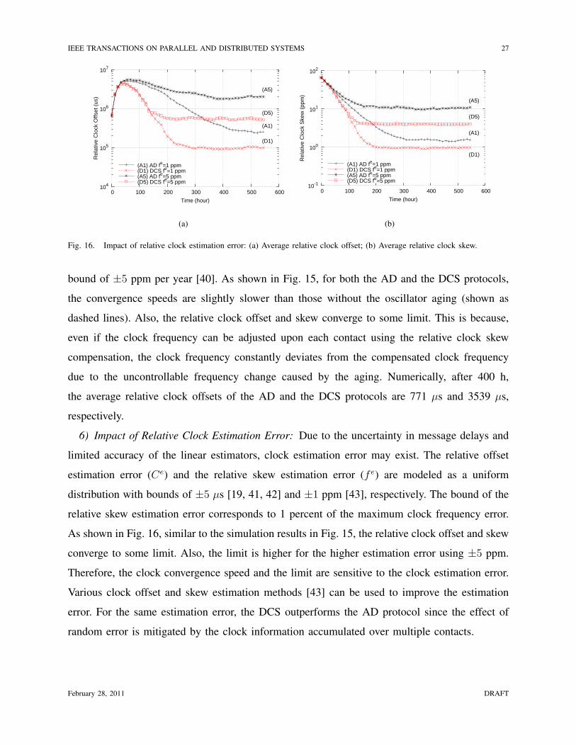
Fig. 16. Impact of relative clock estimation error: (a) Average relative clock offset; (b) Average relative clock skew.
bound of ±5 ppm per year [40]. As shown in Fig. 15, for both the AD and the DCS protocols,
the convergence speeds are slightly slower than those without the oscillator aging (shown as
dashed lines). Also, the relative clock offset and skew converge to some limit. This is because,
even if the clock frequency can be adjusted upon each contact using the relative clock skew
compensation, the clock frequency constantly deviates from the compensated clock frequency
due to the uncontrollable frequency change caused by the aging. Numerically, after 400 h,
the average relative clock offsets of the AD and the DCS protocols are 771 µs and 3539 µs,
respectively.
6) Impact of Relative Clock Estimation Error: Due to the uncertainty in message delays and
limited accuracy of the linear estimators, clock estimation error may exist. The relative offset
estimation error (Ce) and the relative skew estimation error (f e) are modeled as a uniform
distribution with bounds of ±5 µs [19, 41, 42] and ±1 ppm [43], respectively. The bound of the
relative skew estimation error corresponds to 1 percent of the maximum clock frequency error.
As shown in Fig. 16, similar to the simulation results in Fig. 15, the relative clock offset and skew
converge to some limit. Also, the limit is higher for the higher estimation error using ±5 ppm.
Therefore, the clock convergence speed and the limit are sensitive to the clock estimation error.
Various clock offset and skew estimation methods [43] can be used to improve the estimation
error. For the same estimation error, the DCS outperforms the AD protocol since the effect of
random error is mitigated by the clock information accumulated over multiple contacts.
February 28, 2011 DRAFT

IEEE TRANSACTIONS ON PARALLEL AND DISTRIBUTED SYSTEMS 28
VII. CONCLUSION
The clock synchronization is an essential requirement for efficient network protocol operations
in DTNs. To achieve global clock synchronization in DTNs, we have proposed a distributed
asynchronous clock synchronization protocol that uses the relative clock information spread
among nodes. Analytical and simulation results demonstrate that the DCS protocol can achieve
faster convergence speed than existing distributed asynchronous clock synchronization protocols
under various network conditions. A smaller clock error from the DCS protocol can provide
more accurate timing information in data collection from a physical environment and render
sleep scheduling mechanisms more energy efficient.
APPENDIX
PERFORMANCE ANALYSIS OF THE AD PROTOCOL
Since there is no table update in the AD protocol, the update of the clock value Xii(τk) and
clock frequency Yii(τk) of each node can be modeled as
Xii(τk+1) =N∑
l=1l 6=i
1− P0
(N − 1)X il(τk+1) + P0 [Xii(τk) + τYii(τk)] (32)
Yii(τk+1) =N∑
l=1l 6=i
1− P0
(N − 1)Y il(τk+1) + P0Yii(τk), (33)
for i = 1, · · · , N
where X il(τk+1) is the average clock value between nodes i and l if they contact with each other
within τ , given by
X il(τk+1) =[Xii(τk) + τYii(τk)] + [Xll(τk) + τYll(τk)]
2, (34)
and Y il(τk+1) is the average clock frequency between nodes i and l if they contact with each
other within τ , given by
Y il(τk+1) =Yii(τk) + Yll(τk)
2. (35)
Define the system state of the AD protocol at time τk as SAD(τk) = {Xii(τk), Yii(τk)|i = 1,
· · · , N}. Similar to the performance analysis of the DCS protocol, the operation FAD(·) is also
February 28, 2011 DRAFT

IEEE TRANSACTIONS ON PARALLEL AND DISTRIBUTED SYSTEMS 29
defined for the AD protocol. Given the initial clock value Xii(0) = Ci(0) and clock frequency
Yii(0) = fi(0), the system state of the AD protocol at time τk can be calculated as
SAD(τk) = F kAD(SAD(0)). (36)
Then, the performance metrics at time τk, Cavg(τk) and favg(τk), of the AD protocol can be
calculated.
REFERENCES
[1] B. J. Choi and X. Shen, “Distributed Clock Synchronization in Delay Tolerant Networks,” in Proc. IEEE ICC, May. 2010.
[2] “Delay-Tolerant Networking Research Group (DTNRG),” http://www.dtnrg.org/.
[3] K. R. Fall, “A Delay-Tolerant Network Architecture for Challenged Internets,” in Proc. ACM SIGCOMM, Aug. 2003.
[4] “Special Issue on Delay and Disruption Tolerant Wireless Communication Systems,” IEEE J. Select. Areas Commun.,
vol. 26, no. 5, pp. 745–836, June 2008.
[5] H. Jun, M. H. Ammar, and E. W. Zegura, “Power Management in Delay Tolerant Networks: A Framework and Knowledge-
Based Mechanisms,” in Proc. IEEE SECON, Sept. 2005.
[6] B. J. Choi and X. Shen, “Adaptive Asynchronous Clock based Power Saving Protocols for Delay Tolerant Networks,” in
Proc. IEEE GLOBECOM, Nov.–Dec. 2009.
[7] Y. Xi, M. Chuah, and K. Chang, “Performance Evaluation of a Power Management Scheme for Disruption Tolerant
Network,” Lecture Notes in Computer Science, vol. 12, no. 5–6, pp. 370–380, Dec. 2007.
[8] N. Banerjee, M. D. Corner, and B. N. Levine, “An Energy-Efficient Architecture for DTN Throwboxes,” in Proc. IEEE
INFOCOM, April 2007.
[9] K. Romer, “Time Synchronization in Ad Hoc Networks,” in Proc. ACM MobiHoc, Oct. 2001.
[10] J. Burbank, “Network Time Protocol Version 4 Protocol and Algorithms Specification,” IETF, Internet-Draft draft-ietf-ntp-
ntpv4-proto-11, Sept. 2008, work in progress.
[11] W. Su and I. F. Akyildiz, “Time-Diffusion Synchronization Protocol for Wireless Sensor Networks,” IEEE/ACM Trans.
Networking, vol. 13, no. 2, pp. 384–397, 2005.
[12] S. Ganeriwal, R. Kumar, and M. B. Srivastava, “Timing-Sync Protocol for Sensor Networks,” in Proc. ACM SenSys, Nov.
2003.
[13] J. Elson, L. Girod, and D. Estrin, “Fine-Grained Network Time Synchronization Using Reference Broadcasts,” SIGOPS
Oper. Syst. Rev., vol. 36, no. SI, pp. 147–163, 2002.
[14] Q. Ye and L. Cheng, “DTP: Double-Pairwise Time Protocol for Disruption Tolerant Networks,” in Proc. IEEE ICDCS,
June 2008.
[15] J.-P. Sheu, C.-M. Chao, and C.-W. Sun, “A Clock Synchronization Algorithm for Multi-Hop Wireless Ad Hoc Networks,”
in Proc. IEEE ICDCS, June 2004.
[16] D. Zhou and T. H. Lai, “An Accurate and Scalable Clock Synchronization Protocol for IEEE 802.11-Based Multihop Ad
Hoc Networks,” IEEE Trans. Parallel and Distributed System, vol. 18, no. 12, pp. 1797–1808, 2007.
[17] Q. Li and D. Rus, “Global Clock Synchronization in Sensor Networks,” IEEE Trans. Computers, vol. 55, no. 2, pp.
214–226, 2006.
February 28, 2011 DRAFT

IEEE TRANSACTIONS ON PARALLEL AND DISTRIBUTED SYSTEMS 30
[18] P. Sommer and R. Wattenhofer, “Gradient Clock Synchronization in Wireless Sensor Networks,” in Proc. ACM/IEEE IPSN,
April 2009.
[19] C. H. Rentel and T. Kunz, “A Mutual Network Synchronization Method for Wireless Ad Hoc and Sensor Networks,” IEEE
Trans. Mobile Comput., vol. 7, no. 5, pp. 633–646, 2008.
[20] M. Sasabe and T. Takine, “A Simple Scheme for Relative Time Synchronization in Delay Tolerant MANETs,” in Proc.
Int. Conf. Intelligent Networking and Collaborative Systems, Nov. 2009.
[21] A. A. Syed and J. Heidemann, “Time Synchronization for High Latency Acoustic Networks,” in Proc. IEEE INFOCOM,
April 2006.
[22] M. D. Lemmon, J. Ganguly, and L. Xia, “Model-based Clock Synchronization in Networks with Drifting Clocks,” in Proc.
IEEE PRDC, Dec. 2000.
[23] D. P. Bertsekas and J. N. Tsitsiklis, Parallel and Distributed Computation: Numerical Methods. Prentice Hall, 1997.
[24] J. Wolfowitz, “Products of Indecomposable, Aperiodic, Stochastic Matrices,” Proceedings of the American Mathematical
Society, vol. 14, no. 5, pp. 733–737, 1963. [Online]. Available: http://www.jstor.org/stable/2034984
[25] V. Blondel, J. Hendrickx, A. Olshevsky, and J. Tsitsiklis, “Convergence in Multiagent Coordination, Consensus, and
Flocking,” in Proc. IEEE CDC-ECC, Dec. 2005.
[26] W. Zhao, M. Ammar, and E. Zegura, “A Message Ferrying Approach for Data Delivery in Sparse Mobile Ad Hoc
Networks,” in Proc. ACM MobiHoc, May 2004.
[27] R. Shah, S. Roy, S. Jain, and W. Brunette, “Data MULEs: Modeling a Three-tier Architecture for Sparse Sensor Networks,”
in Proc. IEEE SNPA, April 2003.
[28] A. Papoulis, Probability, Random Variables, and Stochastic Processes. McGraw-Hill Companies, 1991.
[29] T. Small and Z. Haas, “Quality of Service and Capacity in Constrained Intermittent-Connectivity Networks,” IEEE Trans.
Mobile Comput., vol. 6, no. 7, pp. 803–814, July 2007.
[30] R. Groenevelt, P. Nain, and G. Koole, “The Message Delay in Mobile Ad Hoc Networks,” Perform. Eval., vol. 62, pp.
210–228, 2005.
[31] P. Denantes, F. Benezit, P. Thiran, and M. Vetterli, “Which Distributed Averaging Algorithm Should I Choose for my
Sensor Network,” in Proc. IEEE INFOCOM, April 2008.
[32] T. Spyropoulos, A. Jindal, and K. Psounis, “An Analytical Study of Fundamental Mobility Properties for Encounter-based
Protocols,” Int. J. Auton. Adapt. Commun. Syst., vol. 1, no. 1, pp. 4–40, 2008.
[33] T. Spyropoulos, K. Psounis, and C. Raghavendra, “Efficient Routing in Intermittently Connected Mobile Networks: The
Multiple-Copy Case,” IEEE/ACM Trans. Networking, vol. 16, no. 1, pp. 77–90, Feb. 2008.
[34] K. Lee, Y. Yi, J. Jeong, H. Won, I. Rhee, and S. Chong, “Max-Contribution: On Optimal Resource Allocation in Delay
Tolerant Networks,” in Proc. IEEE INFOCOM, Mar. 2010.
[35] H. Zhu, L. Fu, G. Xue, Y. Zhu, M. Li, and L. M. Ni, “Recognizing Exponential Inter-Contact Time in VANETs,” in Proc.
IEEE INFOCOM, Mar. 2010.
[36] A. Keranen, J. Ott, and T. Karkkainen, “The ONE Simulator for DTN Protocol Evaluation,” in Proc. ICST SIMUTools,
Mar. 2009.
[37] C. Bettstetter, “On the Minimum Node Degree and Connectivity of a Wireless Multihop Network,” in Proc. ACM MobiHoc,
June 2002.
[38] G. Anastasi, A. Falchi, A. Passarella, M. Conti, and E. Gregori, “Performance Measurements of Motes Sensor Networks,”
in Proc. ACM MSWiM, Oct. 2004.
February 28, 2011 DRAFT

IEEE TRANSACTIONS ON PARALLEL AND DISTRIBUTED SYSTEMS 31
[39] I. Rhee, M. Shin, S. Hong, K. Lee, and S. Chong, “On the Levy-walk Nature of Human Mobility,” in Proc. IEEE
INFOCOM, April 2008.
[40] J. R. Vig, “Introduction to Quartz Frequency Standards,” Army Research Laboratory, Research and Development Technical
Report SLCET-TR-92-1 (Rev. 1), Oct. 1992.
[41] M. Maroti, B. Kusy, G. Simon, and A. Ledeczi, “The Flooding Time Synchronization Protocol,” in Proc. ACM SenSys,
Nov. 2004.
[42] J. Hill and D. Culler, “Mica: A Wireless Platform for Deeply Embedded Networks,” Micro, IEEE, vol. 22, no. 6, pp.
12–24, Nov.-Dec 2002.
[43] E. Serpedin and Q. M. Chaudhari, Synchronization in Wireless Sensor Networks: Parameter Estimation, Peformance
Benchmarks, and Protocols. Cambridge University Press, 2009.
February 28, 2011 DRAFT
Related Documents