IEEE TRANSACTIONS ON MEDICAL IMAGING, VOL. XX, NO. …cchen156.web.engr.illinois.edu/paper/14TMI_DOT.pdf2 IEEE TRANSACTIONS ON MEDICAL IMAGING, VOL. XX, NO. XX, XX XXXX method to solve

IEEE TRANSACTIONS ON MEDICAL IMAGING, VOL. XX, NO. XX, XX XXXX 1

Diffuse optical tomography enhanced by clusteredsparsity for functional brain imaging

Chen Chen, Student Member, IEEE, Fenghua Tian, Hanli Liu, and Junzhou Huang*, Member, IEEE

Abstract—Diffuse optical tomography (DOT) is a noninvasivetechnique which measures hemodynamic changes in the tissuewith near infrared light, which has been increasingly used tostudy brain functions. Due to the nature of light propagation inthe tissue, the reconstruction problem is severely ill-posed. Forlinearized DOT problems, sparsity regularization has achievedpromising results over conventional Tikhonov regularization inrecent experimental research. As extensions to standard sparsity,it is widely known that structured sparsity based methods areoften superior in terms of reconstruction accuracy, when thedata follows some structures. In this paper, we exploit thestructured sparsity of diffuse optical images. Based on thefunctional specialization of the brain, it is observed that thein vivo absorption changes caused by a specific brain functionwould be clustered in certain region(s) and not randomly dis-tributed. Thus, a new algorithm is proposed for this clusteredsparsity reconstruction (CSR). Results of numerical simulationsand phantom experiments have demonstrated the superiorityof the proposed method over the state-of-the-art methods. Anexample from human in vivo measurements further confirmedthe advantages of the proposed CSR method.

Index Terms—Diffuse optical imaging, structured sparsity,clustered sparsity, functional brain imaging.

I. INTRODUCTION

Diffuse optical tomography (DOT) is an emerging techniqueused to study brain functions, which is quickly gaining fa-vorable recognition because of its non-invasive manner andrelatively low cost [1], [2]. This technique uses near infraredlight in a range of 650 to 900 nm, which is sensitive to theabsorptions of oxygenated hemoglobin (HbO2) and deoxy-genated hemoglobin (Hb). The light sources and detectors arearranged on the scalp. The diffused light from the corticallayer of the brain is acquired to form an image of activation.Compared with other neuroimaging modalities, such as func-tional magnetic resonance imaging (fMRI), DOT can providemore comprehensive information of cerebral hemodynamics,while fMRI has better spatial resolution. A recent review ofDOT is given in [3].

One of the main challenges in DOT is the image reconstruc-tion (or inverse problem). Due to the diffusive nature of light

Manuscript received XX XX, 2014; revised XX XX, 2014; accepted XXXX, 2014. Date of publication XX XX, 2014; date of current version XXXX, 2014. Asterisk indicates corresponding author.

C. Chen and J. Huang* are with the Department of Computer Science andEngineering, University of Texas at Arlington, Arlington, TX 76010 USA.Email: [email protected].

F. Tian and H. Liu are with the Department of Bioengineering, theUniversity of Texas at Arlington, Arlington, TX 76010 USA.

Color versions of one or more of the figures in this paper are availableonline at http://ieeexplore.ieee.org.

Digital Object Identifier XXXX

and limited numbers of sources and detectors, the inverse prob-lem is severely ill-posed. In order to make the problem moretractable, it is necessary to make linearization approximation[4], [5], e.g., Rytov approximation. Regularization is often ap-plied to the linear inverse problem to obtain a unique solution.Conventionally, the `2-norm regularization (also known asTikhonov regularization) is the most commonly used methodbecause it can be easily implemented [6]. The drawback is itstendency to over-smooth the image by penalizing large values.Thus, sharp boundaries for the reconstructed images are verydifficult to obtain by the `2-norm regularization.

Since the perturbation from a homogeneous background orreference medium is relatively small in volume and contrast,sparsity of the reconstructed image is generally assumed [7]–[11]. Guided by compressive sensing theory [12], a sparsesignal or image can be recovered from fewer measurementsthan that dictated by Shannon-Nyquist theorem under mildconditions. Sparsity inducing methods have been shown to berepeatedly successful in many real-world applications [13]–[16]. In DOT, `1 norm is first used in [7], [9], [11] to inducesparsity. A more recent work shows that regularization with `p(0 < p < 1) and smooth-`0 norms can improve the results of`1 norm regularization [10], while the inverse problem is moredifficult to solve due to the non-convexity and nonsmoothnessof such norms.

While promising results have been obtained in thesesparsity-inducing methods over the conventional `2 norm reg-ularization, accurate reconstruction of diffuse optical images isstill challenging. First, experiments often involve noise, whilestandard sparsity based methods are often not robust to noise,e.g. those in our later simulations. True signals are difficultto distinguish from significant noise, as the noise may alsosatisfy the sparsity assumption. Second, based on compressivesensing theory, the minimal number of measurements forsuccessful recovery is required to be O(K + K log(N/K)),where K is the number of non-zero components and N is thelength of the signal. Limited by the number of measurementsin DOT, these standard sparsity based methods may failwhen the image is less sparse (i.e., K is larger). Fortunately,such limitations of standard sparsity have been overcome inadvanced sparsity techniques called structured sparsity [17],[18]. According to structured sparsity theories [17]–[19], fewermeasurements are required for signals with structured sparsitythan those with standard sparsity, or the recovery accuracy canbe improved with the same number of measurements. Also,structured sparsity based methods are often more robust tonoise. However, for different types of data, discovering theunderlying structures of the data and developing an efficient

2 IEEE TRANSACTIONS ON MEDICAL IMAGING, VOL. XX, NO. XX, XX XXXX

method to solve the corresponding problem is still open toquestions. In this study, we aim to improve DOT based onstructured sparsity.

The diffuse optical images do have some special structuresif we look at the brain features in biology. It is widely knownthat human actions correspond to certain regions of brainactivation. For example, brain state changes specifically inthe dorsal medial prefrontal area during Vipassana meditation[20]. These changes of brain state only take place in a region orregions but are not randomly distributed over the whole brain,which will make the change of absorption have a clusteredappearance. In contrast to previous works that use no prioriinformation other than sparsity, we propose a new methodto improve the reconstruction by exploiting this clusteredstructure. We call this method clustered sparsity reconstruc-tion (CSR). The clustered sparsity problem is modeled withconvex programming and solved by a new algorithm based onthe Fast Iterative Shrinkage-Thresholding Algorithm (FISTA)framework [21]. Comprehensive experimental results havedemonstrated significant improvements achieved by our CSRmethod when compared with previous works.

II. THEORY

A. Regularization for DOT

The relative change in optical density is measured byeach source-detector (S-D) pair. Photon propagation in humantissue is mathematically described by the Boltzmann transportequation [7]. Following previous work [22], we assume thebackground optical parameters are known in this study. There-fore, the reconstruction problem in DOT can be simplified bythe linear Rytov approximation [7], [9]:

Ax = b, (1)

where b ∈ Rm×1 is the vector of measured relative light densi-ty changes; x ∈ Rn×1 represents an image (after vectorizing)of4µa (i.e., the change of absorption coefficient); A ∈ Rm×nis the forward sensing matrix referring to the sensitivity ofpixels with different S-D pairs. Due to the limitation on thenumber of S-D pairs and the diffusive nature of light, thisproblem is severely ill-posed, i.e., m << n. To obtain a uniquesolution, the `2-norm regularization is widely used and theobjective function becomes:

x = argminx{12||Ax− b||22 + λ||x||22}, (2)

where λ is a positive parameter and can be selected by theL-curve method [23]. To overcome the over-smoothing by `2-norm regularization, many recent methods have been proposedto exploit the sparsity of the reconstructed image [7], [9], [10],[24]. Sparsity-inducing norms, e.g. `1, `p (0 < p < 1) andsmooth-`0 norms, are used for regularization instead of `2norm:

x = argminx{12||Ax− b||22 + λ||x||pp}, (3)

x = argminx{12||Ax− b||22 + λ||x||0} (4)

where the `0 norm is approximated with the Gaussian function.Promising results have been obtained using these methods.

However, these standard sparsity based methods only exploitthe sparseness of the reconstructed image, while the corre-lations or structures of the non-zero values have not beenutilized.

B. Structured SparsityCompressive sensing theory [12] provides a theoretical

guarantee for robust recovery with standard sparsity (e.g.`1 norm). Under mild conditions, it has been proven thatO(K+K log(N/K)) measurements are required for success-ful recovery with high probability, where K is the number ofnonzero components and N is the total number of components.However, for DOT problems, the number of measurementsis limited by physical reasons, e.g., the diffusive nature oflight and the size of source-detectors. In some cases wherethe images are less sparse, i.e., K is relatively large to N , theperformance of standard sparsity based methods (e.g., thosementioned above) cannot be guaranteed.

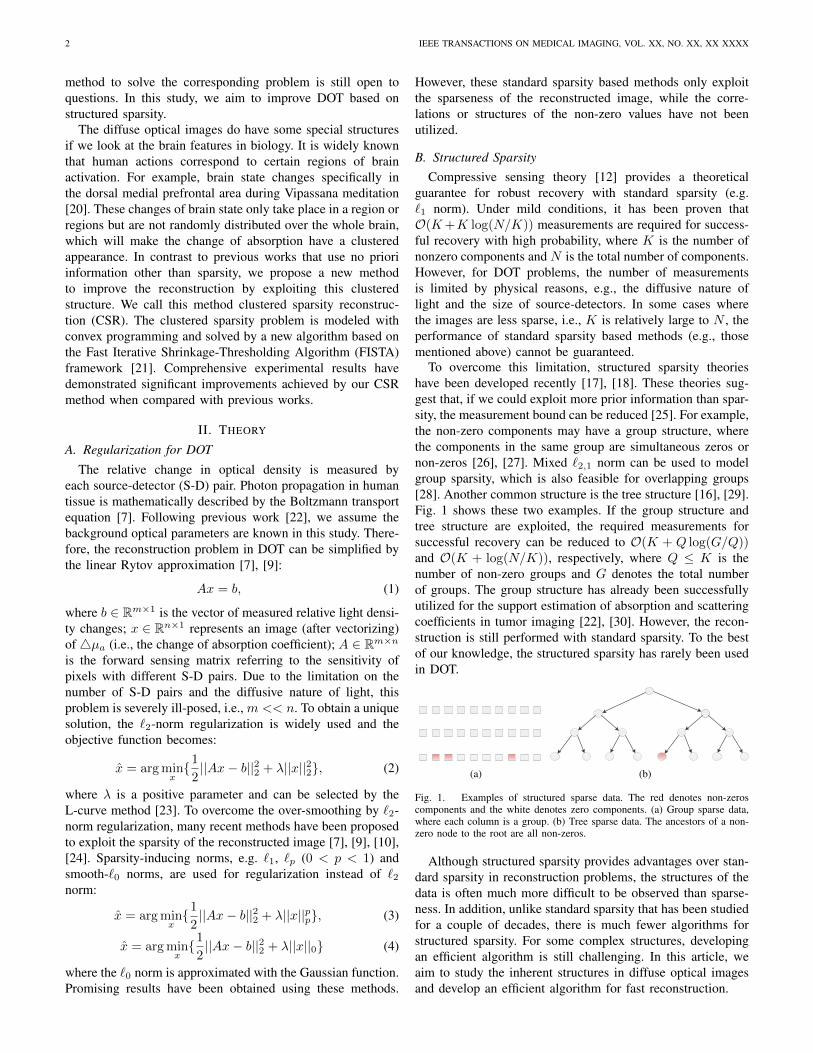
To overcome this limitation, structured sparsity theorieshave been developed recently [17], [18]. These theories sug-gest that, if we could exploit more prior information than spar-sity, the measurement bound can be reduced [25]. For example,the non-zero components may have a group structure, wherethe components in the same group are simultaneous zeros ornon-zeros [26], [27]. Mixed `2,1 norm can be used to modelgroup sparsity, which is also feasible for overlapping groups[28]. Another common structure is the tree structure [16], [29].Fig. 1 shows these two examples. If the group structure andtree structure are exploited, the required measurements forsuccessful recovery can be reduced to O(K + Q log(G/Q))and O(K + log(N/K)), respectively, where Q ≤ K is thenumber of non-zero groups and G denotes the total numberof groups. The group structure has already been successfullyutilized for the support estimation of absorption and scatteringcoefficients in tumor imaging [22], [30]. However, the recon-struction is still performed with standard sparsity. To the bestof our knowledge, the structured sparsity has rarely been usedin DOT.

(a) (b)

Fig. 1. Examples of structured sparse data. The red denotes non-zeroscomponents and the white denotes zero components. (a) Group sparse data,where each column is a group. (b) Tree sparse data. The ancestors of a non-zero node to the root are all non-zeros.

Although structured sparsity provides advantages over stan-dard sparsity in reconstruction problems, the structures of thedata is often much more difficult to be observed than sparse-ness. In addition, unlike standard sparsity that has been studiedfor a couple of decades, there is much fewer algorithms forstructured sparsity. For some complex structures, developingan efficient algorithm is still challenging. In this article, weaim to study the inherent structures in diffuse optical imagesand develop an efficient algorithm for fast reconstruction.

CHEN et al.: DIFFUSE OPTICAL TOMOGRAPHY ENHANCED BY CLUSTERED SPARSITY FOR FUNCTIONAL BRAIN IMAGING 3

(a) (b) (c)

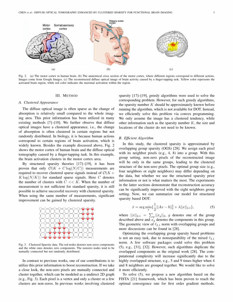
Fig. 2. (a) The motor cortex in human brain. (b) The anatomical cross section of the motor cortex, where different regions correspond to different actions.Images come from Google Images. (c) The reconstructed diffuse optical image of brain activity caused by a finger-tapping task. Yellow color represents theactivated brain region, while red color indicates the maximal activation within the region.

III. METHOD

A. Clustered Appearance

The diffuse optical image is often sparse as the change ofabsorption is relatively small compared to the whole imag-ing area. This prior information has been utilized in manyexisting methods [7]–[10]. We further observe that diffuseoptical images have a clustered appearance, i.e., the changeof absorption is often clustered in certain regions but notrandomly distributed. In biology, it is because human actionscorrespond to certain regions of brain activation, which iswidely known. Besides the example discussed above, Fig. 2shows the motor cortex of human brain and the diffuse opticaltomography caused by a finger-tapping task. In this example,the brain activation clusters in the motor cortex area.

By structured sparsity theories [17]–[19], it has beenproven that only O(K + C log(N/C)) measurements arerequired to recover clustered sparse signals instead of O(K+K log(N/K)) for standard sparse signals. Here C denotesthe number of clusters with C << K. When the number ofmeasurement is not sufficient for standard sparsity, it is stillpossible to achieve successful recovery with clustered sparsity.When using the same number of measurements, significantimprovement can be gained by clustered sparsity.

Fig. 3. Clustered Sparsity data. The red nodes denotes non-zeros componentsand the white ones denotes zero components. The nonzero nodes tend to bemutually connected but not randomly distributed.

In contrast to previous works, one of our contributions is toutilize this prior information to boost reconstruction. If we takea close look, the non-zero pixels are mutually connected andcluster together, which can be modeled as a undirect 2D graph(e.g., Fig. 3). Each pixel is a vertex and only a cluster or a fewclusters are non-zeros. In previous works involving clustered

sparsity [17]–[19], greedy algorithms were used to solve thecorresponding problem. However, for such greedy algorithms,the sparsity number K should be approximately known beforerunning the algorithm, which is not available for DOT. Instead,we efficiently solve this problem via convex programming.We only assume the image has a clustered tendency, whileother information such as the sparsity number K, the size andlocations of the cluster do not need to be known.

B. Efficient Algorithm

In this study, the clustered sparsity is approximated byoverlapping group sparsity (OGS) [28]. We assign each pixelwith its neighbor pixels (e.g., 4, 8) into a group. With thisgroup setting, non-zero pixels of the reconstructed imagewill be only in the same groups, leading to the clusteredstructure of the non-zero pixels. The optimal group size (e.g.,four neighbors or eight neighbors) may differ depending onthe data, but whether we use the structured sparsity priorinformation or not is what matters the most. The experimentsin the latter sections demonstrate that reconstruction accuracycan be significantly improved with the eight neighbors groupsetting. Now, we can summarize our model for structuredsparsity based DOT:

x = argminx{12||Ax− b||22 + λ||x||2,1}, (5)

where ||x||2,1 =∑g ||xg||2, g denotes one of the group

described above and xg denotes the components in this group.The geometric view of `2,1 norm with overlapping groups andmore discussions can be found in [28].

Optimizing the overlapping group sparsity based problemsis not an easy task, due to nonseparability of the mixed `2,1norm. A few software packages could solve this problem(5), e.g., [31], [32]. However, such algorithms duplicate theoverlapped components as the original work [28]. The com-putational complexity will increase significantly due to thehighly overlapped structure, e.g., 5 and 9 times higher when 4and 8 neighbors are grouped together. We would like to solveit more efficiently.

To solve (5), we propose a new algorithm based on theFISTA [21] framework, which has been proven to reach theoptimal convergence rate for first order gradient methods.

4 IEEE TRANSACTIONS ON MEDICAL IMAGING, VOL. XX, NO. XX, XX XXXX

The whole algorithm is summarized in Algorithm 1. We callit as clustered sparsity reconstruction (CSR). For the firststep, f(x) = 1

2 ||Ax − b||22, and ∇f(x) = AT (Ax − b)denotes its gradient which has Lipschitz constant L. Thesmallest Lipschitz constant L can be selected based on themaximum eigenvalue of ATA. AT denotes the transpose of A.In the original FISTA algorithm for `1 norm regularization, thesecond step has a closed form solution by soft-thresholding.However, due to the nonsmoothness and nonseparability ofthe overlapped `2,1 norm, there is no closed form solution forthe OGS thresholding/denosing problem in the second step.We apply the reweighted least squares algorithm [33]–[35]to solve it. Finally, each xk is updated by the results in theprevious two iterations to accelerate the convergence.

Algorithm 1 Clustered Sparsity Reconstruction (CSR)Purpose: minx{ 12 ||Ax− b||

22 + λ||x||2,1}

Input: ρ = 1L , λ, t1 = 1, y0 = x0

for k = 1 to N do1) s = xk − ρ∇f(xk)2) yk = argminy{ 1

2ρ‖y − s‖2 + λ‖y‖2,1}

3) tk+1 = [1 +√

1 + 4(tk)2]/2

4) xk+1 = yk + tk−1tk+1 (y

k − yk−1)end for

The OGS thresholding algorithm is listed in Algorithm2. conv(x, J) denotes the convolution operation for x withtemplate J and ”.” denotes the element-wise operations. Jdepends on our group setting that has been discussed before.Note that both x and b need to be reshaped in 2D in orderto apply convolutions. Compared with standard OGS solvers[31], [32] with O(NS) complexity, this algorithm only costsO(N logS), where S is the size of each group.

Algorithm 2 OGS ThresholdingPurpose: minx{ 12 ||x− b||

22 + λ||x||2,1}

Input: λ, x0 = b, J = [1, 1, 1; 1, 1, 1; 1, 1, 1]for k = 1 to N do

1) r =√conv(x.× x, J)

2) x = b./[1 + λ ∗ conv(r, J)]end for

IV. EXPERIMENT

A. Simulation

Simulations are conducted using the PMI Toolbox [36].Theprobe geometry of these simulations and later phantom ex-periments is the same as that in previous work [37]. Thenumber of measurements is m = 188, and the field of view(FOV) is 6cm × 6cm with resolution 61 × 61 pixels. Theoptical properties of the medium are absorption coefficientµa = 0.08cm−1 and reduced scattering coefficient µ′s =8.8cm−1. The objects (two spheres of 1-cm diameter) havethe same scattering coefficient as the medium, and a higherabsorption coefficient µa = 0.3cm−1. The sensitivity matrixA is generated by Rytov approximation [9]. Random Gaussiannoise with standard derivation σ is added into the measurement

vector b. Root-mean-square error (RMSE) and contrast-to-noise ratio (CNR) are used as metrics for evaluation. Fromthe definition, the reconstructed image with larger CNR meansbetter performance. As suggested in [10], p in the `p normregularization is set as 0.5. There is an additional `2 termcombined in the software of smooth `0 method. We set thisparameter as the best value of that in the `2 norm regularizationmethod.

10−10

10−8

10−6

10−4

10−2

100

0.02

0.03

0.04

0.05

0.06

0.07

0.08

0.09

0.1

λ

RM

SE

L2

L0.5

L0

L1

Proposed

Fig. 4. Reconstruction performance of different algorithms when σ = 0.0004(SNR = 20.79 dB).

The RMSEs for different λ are presented at Fig. 4 whenσ = 0.0004. This corresponds to a signal-to-noise ratio (SNR)of 20.79 dB. Compared with previous methods, smaller errorsare achieved by the proposed method with a proper λ, whichcoincides with the structured sparsity theories. Both the `2norm regularization [38] and the proposed method are lesssensitive to the parameter setting.

Fig. 5 (a) presents the reconstruction results in terms ofabsorption change (4µa, cm−1) at the optimal parameters foreach algorithm when σ = 0.0004. All the reconstructed imagesare shown at the same scale. The absorbers reconstructed by`2 norm regularization have a low contrast to the backgrounddue to over-smoothing. Sparse results are achieved by smooth`0, `0.5 [10] and `1 norm regularization [9], which have muchhigher contrasts compared with the previous one. However,these norms only encourage sparsity and have no other con-straints on the locations of the non-zero values. The absorberson the images are slightly distorted and distributed, e.g., thoseby the `1 norm and `0.5 norm regularization. Our method notonly induces sparsity, but also encourage the non-zero valuesto be clustered. The cross sections of these recovered imagesat x = 0 are shown in Fig. 5 (b). Compared to the ground-truthimage, the result obtained by the `2 norm has smaller pixelvalues, while those reconstructed by `1 norm and smooth `0norm have significantly larger pixel values. It is consistent withour visual observations of Fig. 5 (a).

We also validate these algorithms with increased noise.When we gradually increase σ, the reconstructed absorbersof the existing sparsity based methods tend to be severelydistorted, while that by the conventional `2 norm regularizationhas a very low contrast. Fig. 6 presents the results whenσ = 0.002 (SNR = 7.66 dB). We use different color barsto show these results. Even with big noise, the result given by

CHEN et al.: DIFFUSE OPTICAL TOMOGRAPHY ENHANCED BY CLUSTERED SPARSITY FOR FUNCTIONAL BRAIN IMAGING 5

-2 0 2-3

-2

-1

0

1

2

3

-2 0 2-3

-2

-1

0

1

2

3

-2 0 2-3

-2

-1

0

1

2

3

0

0.1

0.2

0.3

0.4

-2 0 2-3

-2

-1

0

1

2

3

-2 0 2-3

-2

-1

0

1

2

3

-2 0 2-3

-2

-1

0

1

2

3

0

0.1

0.2

0.3

0.4L2 L0.5

Smooth L0 L1 CSR (Proposed)

Ground Truthcm

cm

cm

cm

cm

cm

cm

cm

cm

cm

cm

cm

(a)

0 10 20 30 40 50 60 70−0.05

0

0.05

0.1

0.15

0.2

0.25

0.3

0.35

0.4

0.45

Pixel Index

Pix

el V

alue

(cm

−1 )

Ground TruthL

2

L0.5

L0

L1

Proposed

(b)

Fig. 5. (a) The ground-truth image and the reconstructed images of 4µa in cm−1 based on simulations, where σ = 0.0004 (SNR = 20.79 dB). (b) Crosssections of the absorbers at x = 0, which is indicated by the white arrows in (a).

our CSR method is only sightly distorted and the shapes ofthe absorbers can be clearly observed. As the higher accuracyof our method can be clearly observed in this figure, wedo not compare the cross sections of different images here.Comparing results with a different power of noise in Figs. 5and 6, the standard sparsity based methods (`0.5, `1, and `0norm regularization) are not robust to noise.

-2 0 2-3

-2

-1

0

1

2

3

0

0.05

0.1

0.15

-2 0 2-3

-2

-1

0

1

2

3

-0.5

0

0.5

1

-2 0 2-3

-2

-1

0

1

2

3

-0.2

0

0.2

0.4

0.6

-2 0 2-3

-2

-1

0

1

2

3

0.2

0.4

0.6

0.8

1

1.2

1.4

-2 0 2-3

-2

-1

0

1

2

3

0

0.05

0.1

0.15

0.2

-2 0 2-3

-2

-1

0

1

2

3

-0.02

0

0.02

0.04

L2 L0.5

Smooth L0 L1 CSR (Proposed)

Ground Truthcm

cm

cm

cm

cm

cm

cm

cm

cm

cm

cm

cm

Fig. 6. The ground-truth image and the reconstructed images from thesimulation (4µa in cm−1), where σ = 0.002 (SNR = 7.66 dB).

To quantitatively validate the above conclusion, the recon-struction errors of different methods are presented in Fig.7 with different levels of noise. To reduce randomness, werun each method at each setting 20 times, and the averageresults are reported here. It can be clearly observed thatthe conventional `2 norm method and the proposed methodare more robust to noise, while the standard sparsity basedmethods using `0.5 norm and `1 norm are sensitive to noise.The proposed CSR method consistently outperforms all of theother methods. These results further confirm the advantagesof the proposed CSR method.

8 10 12 14 16 18 20 220.02

0.025

0.03

0.035

0.04

0.045

0.05

0.055

0.06

0.065

0.07

SNR

RM

SE

L2

L0.5

L0

L1

Proposed

Fig. 7. The reconstruction errors of different methods with various levels ofnoise.

B. Phantom

We further conducted experiments to validate our methodusing laboratory tissue phantoms. The experiment environmentwas the same as that in previous work [37]. A large tank(approximately 15 × 10 × 10cm3) was used to contain thephantom. The walls of this tank were covered by black tapeso that no light was reflected. The phantom had an absorptioncoefficient of µa = 0.08cm−1 and a reduced scatteringcoefficient of µ′s = 8.8cm−1. A 1-cm diameter sphericalabsorber with µa = 0.3cm−1 and the same reduced scatteringcoefficient was placed around the x-axis and 3cm below thesurface of the phantom. The measured data with and withoutthe absorber were respectively acquired by all 188 channels.Keeping the experimental setup, we then place two sphericalabsorbers with 1cm diameter around the y-axis at the samedepth to conduct another experiment.

In previous methods [9], [38], the L-curve method [23] wasused to select the parameters. However, such an approachoften does not lead to the optimal parameters [39], [40]. Inthis study, we first selected a small range of the parameters

6 IEEE TRANSACTIONS ON MEDICAL IMAGING, VOL. XX, NO. XX, XX XXXX

-2 0 2-3

-2

-1

0

1

2

3

0

0.02

0.04

0.06

-2 0 2-3

-2

-1

0

1

2

3

-0.3

-0.2

-0.1

0

0.1

0.2

0.3

-2 0 2-3

-2

-1

0

1

2

3

0

0.2

0.4

0.6

0.8

1

-2 0 2-3

-2

-1

0

1

2

3

0

0.05

0.1

0.15

0.2

0 20 40 60 80-0.5

0

0.5

1

1.5

Pixel Index

Pix

el V

alu

e (c

m-1

)

L2

L0.5

L0

L1

Proposed

L2 L0.5 Smooth L0 cmcmcm

L1 CSR (Proposed)

cmcm cm

cmcm

cmcm

-2 0 2-3

-2

-1

0

1

2

3

0

0.05

0.1

0.15

0.2

0.25

Fig. 8. Reconstructed images of a single absorber (4µa in cm−1). Dashed circles indicate the actual size of the object. The right bottom panel shows thecross sections of different images at the maximum pixel value, which are indicated by the arrows in the reconstructed images. The black solid line indicatesthe maximum 4µa caused by the actual absorber.

by the L-curve method, and then the final parameter wasselected in this range with user’s adjustment. A sparser solu-tion with fewer clusters is preferred. We list the parametersof different methods in Table I, which are used for bothphantom experiments. An adaptive method proposed recentlymay alleviate this parameter tuning process [41]. Interestingly,we find these parameter settings are consistent with thosein Fig. 4. It indicates another way to tune the parametersin clinic applications. The parameters tuned in some knowntasks may be used for other tasks with the same experimentalenvironment.

TABLE ITHE PARAMETER SETTING FOR THE DIFFERENT METHODS.

`2 `0.5 smooth `0 `1 CSRλ 6.7× 10−6 10−7 0.05 6× 10−7 10−6

Figs. 8 and 9 present the reconstruction results for thesetwo phantom experiments. Due to their significantly differentreconstructed values, separate color bars are used. Since weknow the actual size of the absorbers, the absorbers recon-structed by the `2 norm look dispersive, with larger areasand smaller intensity. We could find that the results obtainedby the `0.5 norm, smooth `0 norm and `1 norm tend to besmaller than the ground-truth. Reconstruction of the seconddata (Fig. 9) is quite difficult as it is less sparse. The trueabsorbers are hard to be distinguished by `0.5 and `1 normmethods. If we take a close look, the images recovered by the`2 norm and smooth `0 norm contain pixels of negative values.

This may result in cross-talk in actual functional brain study[42]. Quantitative comparisons of these experiments are listedin Table II, which is consistent with our visual observations.Based on the simulations results and the above analysis, theabsorbers recovered by our CSR method should be the closestone to the ground-truth in terms of object area and intensity.One of the reasons is that our structured sparsity based methodis less sensitive to noise. The random noise often does notfollow the structures of the true signal, while it is hard todistinguish using the standard sparsity based methods.

TABLE IITHE CNRS OF DIFFERENT PHANTOM RECONSTRUCTION RESULTS.

`2 `0.5 smooth `0 `1 CSRFig. 8 4.69 8.34 10.71 3.66 14.03Fig. 9 3.36 4.14 5.32 3.07 6.70

C. Functional Human Brain Imaging

We have validated that the proposed CSR outperformsprevious methods on the simulated data and phantom data.Our next task is to show how we applied the proposed methodon functional brain imaging. A well known motor task [43](i.e., finger-tapping) is used here to observe motor cortexactivation. We follow the same protocol as that in [44] and themeasurements were acquired by a multichannel, continuous-wave NIRS system (CW-5, Techen Inc., Milford, MA) [45].Following a fixed rhythm, the subjects were instructed tosimultaneously tap four fingers (except thumb) up and down

CHEN et al.: DIFFUSE OPTICAL TOMOGRAPHY ENHANCED BY CLUSTERED SPARSITY FOR FUNCTIONAL BRAIN IMAGING 7

-2 0 2-3

-2

-1

0

1

2

3

0.1

0.2

0.3

0.4

-2 0 2-3

-2

-1

0

1

2

3

-0.05

0

0.05

0.1

0.15

-2 0 2-3

-2

-1

0

1

2

3

0.1

0.2

0.3

0.4

0.5

0.6

0.7

-2 0 2-3

-2

-1

0

1

2

3

-0.2

0

0.2

0.4

0.6

0.8

1

-2 0 2-3

-2

-1

0

1

2

3

0

0.5

1

1.5

L2 L0.5 Smooth L0 cmcmcm

L1 CSR (Proposed)

cmcm cm

cmcm

cmcm

0 20 40 60 80-0.5

0

0.5

1

1.5

2

Pixel Index

Pix

el V

alu

e (c

m-1

)

L2

L0.5

L0

L1

Proposed

Fig. 9. Reconstructed images of two separated absorbers (4µa in cm−1). Dashed circles indicate the actual sizes of the objects. The right bottom panelshows the cross sections of different images at the maximum pixel value, which are indicated by the white arrows in the reconstructed images. The blacksolid line indicates the maximum 4µa caused by the actual absorbers.

without moving the wrist and arm. Light of 690 nm and at830 nm wavelengths were emitted from sources to measurethe changes in concentrations of oxy- and deoxy- hemoglobin.The image covered a space of 20.32× 5.84cm2 in the brain.The reconstructed images (with 41× 13 pixels) were sliced atZ = −1.5cm depth.

We randomly selected one of the eight subjects that was re-ported in [44]. With the same measurements, we reconstructedthe images with different methods, which contain `2 norm, `0.5norm [10], smooth `0 norm [10], `1 norm [9] regularizationand the proposed CSR. The λ in our method was selected as7.9×10−4. Those results are presented in Fig. 10 on the samescale.

The images reconstructed by all methods had brain activa-tion on the lower right side. This is expected due to the lefthand finger tapping (contra-lateral activation) of the subject.Enlarged activation areas were obtained by the `2 norm andsmooth `0 norm regularization (the first row and the thirdrow of Fig. 10), while the remaining images showed smalleractivation areas. If comparing the sparsity inducing methods(i.e., `0.5 norm, smooth `0 norm, `1 norm with the proposedmethod), the proposed method and `0 norm produced morelocalized images. In addition, it is obvious that the images ob-tained by our CSR method (the last row of Fig. 10) had muchhigher contrasts than those obtained by `0 norm. Consideringthe shapes of different results, our method provided a moreconcentrated and accurate result. Comparing the reconstructionresults of oxyhemoglobin and deoxyhemoglobin (i.e, the firstcolumn and the second column), it seems that our method can

potentially reduce the cross-talk [42]. These results confirmsthe benefit of our method in functional human brain studies.

V. DISCUSSION AND CONCLUSION

In this study, we proposed to use structured sparsity toimprove the reconstruction accuracy of DOT. More precisely,the clustered prior information was utilized by the mixed`2,1 norm regularization. This was motivated by the fact thatfunctional brain activation is often localized in some specialregion(s) but not randomly distributed. Before this study,the clustered sparsity had already been successfully used incompressed sensing and computer vision [46]. It leads toseveral advantages: 1) improving the reconstruction accuracywith the same number of measurements; 2) maintaining stablerecovery when the measurements are not sufficient for standardsparsity (e.g., by `1 norm); 3) enhancing the robustness tonoise and preventing artifacts in the background. By structuredsparsity theories [17]–[19], it has been proved that onlyO(K + C log(N/C)) measurements are required to recoverclustered sparse signals instead of O(K +K log(N/K)) forstandard sparse signals. Here C denotes the number of clusters,which is significantly smaller than the number of non-zeropixels K. There is no additional information (e.g., shape, size,location of the absorbers) required for the proposed algorithm.These are why it could facilitate diffuse optical imaging withhigh accuracy.

Numerical simulation and phantom experiments have val-idated the effectiveness of our method when comparedwith conventional and recent algorithms. Qualitative analysis

8 IEEE TRANSACTIONS ON MEDICAL IMAGING, VOL. XX, NO. XX, XX XXXX

Left LeftRight Right

-10 -5 0 5 10

X (cm)

-10 -5 0 5 10

X (cm)

-10 -5 0 5 10

X (cm)

-10 -5 0 5 10

X (cm)

-10 -5 0 5 10

X (cm)

-10 -5 0 5 10

X (cm)

-10 -5 0 5 10

X (cm)

-10 -5 0 5 10

X (cm)

-10 -5 0 5 10

X (cm)

-10 -5 0 5 10

X (cm)

Y (

cm) 2

0

-2Y

(cm

) 2

0

-2

Y (

cm) 2

0

-2

Y (

cm) 2

0

-2

Y (

cm) 2

0

-2

Y (

cm) 2

0

-2

Y (

cm) 2

0

-2

Y (

cm) 2

0

-2

Y (

cm) 2

0

-2Y

(cm

) 2

0

-2

-0.02

-0.01

0

0.01

0.02

-0.02

-0.01

0

0.01

0.02

-0.02

-0.01

0

0.01

0.02

-0.02

-0.01

0

0.01

0.02

-0.02

-0.01

0

0.01

0.02

Fig. 10. 2D slices (1.5 cm below the scalp surface) of reconstructed human brain images induced by a finger tapping task. Left column: the images reconstructedfor increased oxy-hemoglobin concentration (arbitrary unit). Right column: the images reconstructed for decreased deoxy-hemoglobin concentration (arbitraryunit). From the first row to the last row, the images are reconstructed using `2 norm, `0.5 norm, smooth `0 norm, `1 norm and the proposed method,respectively. The figure is best viewed on screen, rather than in print.

demonstrated that out method can outperform existing ap-proaches up to 30% in terms of CNR. The superior perfor-mance of our method was further confirmed on in vivo data.Our method can recover images with the fewest artifacts andbest contrasts in the expected region. Practical applicationscan benefit from the proposed CSR method with little or norevision on the hardware.

Currently, parameter selection is still an open active researcharea for DOT. To the best of our knowledge, there is noefficient way to accurately select the optimal regularizationparameter or parameters for each algorithm. For this reason,an algorithm that has fewer parameters and is not sensitiveto the parameters is preferred. The `1 norm and `0.5 normbased methods are very sensitive to parameter settings, asillustrated by their sharp curves in Fig. 4. We used the originalFISTA algorithm to solve the `1 norm regularization problemand ran sufficient iterations until the algorithm converged.The human brain imaging results seem to be better if thestopping criteria are controlled manually [11], e.g., by settingthe number of Newton iterations. However, multiple parameterselection is a drawback of the algorithm. A similar issueis also in the method of smooth `0 norm regularization,where an additional `2 norm regularization term is included

in the software. By contrast, there is only one non-sensitiveparameter λ in our method. We have made our best effortto select the optimal parameters for different methods forfair comparisons. Although the parameters for the previousmethods may not be exactly optimal, the experimental resultsare sufficient to demonstrate the benefit of our method, whichcan achieve substantial improvement in image reconstructionwith only one non-sensitive parameter.

All experiments are conducted using MATLAB on a desktopwith 3.4GHz Intel core i7 3770 CPU. The reconstructionspeed of our CSR method is slightly slower than the `1norm regularization method, due to the more difficult problemwith overlapping groups. In the phantom experiments, thereconstruction times of the `2 norm, `0.5 norm, smooth `0norm, `1 norm based methods and the proposed method arearound 3 seconds, 26 seconds, 2 seconds, 14 seconds and 23seconds, respectively. Due to the linear approximation, suchreconstruction speed is quite acceptable.

Although the proposed CSR method has achieved promisingresults, some applications in DOT is still very challenging. D-ifferent from functional brain imaging, tumor imaging involvesthe problem to reconstruct both scattering and absorptioncoefficients [22]. The current work cannot be directly applied

CHEN et al.: DIFFUSE OPTICAL TOMOGRAPHY ENHANCED BY CLUSTERED SPARSITY FOR FUNCTIONAL BRAIN IMAGING 9

to such case. In some scenarios, such as breast imaging [47],the image may not be sparse. Some sparsity transformationmay be required, e.g., the total variation [22]. Future workwill focus on extending the proposed method in such cases.

REFERENCES

[1] D. A. Boas, A. M. Dale, and M. A. Franceschini, “Diffuse opticalimaging of brain activation: approaches to optimizing image sensitivity,resolution, and accuracy,” Neuroimage, vol. 23, pp. S275–S288, 2004.

[2] A. Villringer and B. Chance, “Non-invasive optical spectroscopy andimaging of human brain function,” Trends in neurosciences, vol. 20,no. 10, pp. 435–442, 1997.

[3] T. Durduran, R. Choe, W. Baker, and A. Yodh, “Diffuse optics for tissuemonitoring and tomography,” Rep. Prog. Phys., vol. 73, no. 7, p. 076701,2010.

[4] A. C. Kak and M. Slaney, Principles of computerized tomographicimaging. AC Kah and Malcolm Slaney, 1999.

[5] S. R. Arridge and J. C. Schotland, “Optical tomography: forward andinverse problems,” Inverse Probl., vol. 25, no. 12, p. 123010, 2009.

[6] M. Guven, B. Yazici, X. Intes, and B. Chance, “Diffuse optical tomog-raphy with a priori anatomical information,” Phys. Med. & Biol, vol. 50,no. 12, p. 2837, 2005.

[7] N. Cao, A. Nehorai, and M. Jacobs, “Image reconstruction for dif-fuse optical tomography using sparsity regularization and expectation-maximization algorithm,” Opt. Express, vol. 15, pp. 13 695–13 708,2007.

[8] J. Ye, S. Lee, and Y. Bresler, “Exact reconstruction formula for diffuseoptical tomography using simultaneous sparse representation,” in ProcIEEE Int. Symp. Biomed. Imaging. (ISBI), 2008.

[9] M. Suzen, A. Giannoula, and T. Durduran, “Compressed sensing indiffuse optical tomography,” Opt. Express, vol. 18, no. 23, pp. 23 676–23 690, 2010.

[10] J. Prakash, C. Shaw, R. Manjappa, R. Kanhirodan, and P. K. Yalavarthy,“Sparse recovery methods hold promise for diffuse optical tomographicimage reconstruction,” IEEE J. Sel. Topics Quantum Electron., vol. 20,no. 2, p. 6800609, 2014.

[11] V. C. Kavuri, Z.-J. Lin, F. Tian, and H. Liu, “Sparsity enhanced spatialresolution and depth localization in diffuse optical tomography,” Biomed.Opt. Express, vol. 3, no. 5, p. 943, 2012.

[12] E. Candes, J. Romberg, and T. Tao, “Robust uncertainty principles: Exactsignal reconstruction from highly incomplete frequency information,”IEEE Trans. Inf. Theory, vol. 52, no. 2, pp. 489–509, 2006.

[13] M. Lustig, D. Donoho, and J. Pauly, “Sparse MRI:The application ofcompressed sensing for rapid MR imaging,” Magn. Reson. Med., vol. 58,pp. 1182–1195, 2007.

[14] Y. Zheng, E. Daniel, A. A. Hunter III, R. Xiao, J. Gao, H. Li, M. G.Maguire, D. H. Brainard, and J. C. Gee, “Landmark matching basedretinal image alignment by enforcing sparsity in correspondence matrix,”Med. Image Anal., vol. 18, no. 6, pp. 903–913, 2014.

[15] J. Huang, S. Zhang, H. Li, and D. Metaxas, “Composite splittingalgorithms for convex optimization,” Comput. Vis. Image. Und., vol.115, no. 12, pp. 1610–1622, 2011.

[16] C. Chen and J. Huang, “Compressive sensing MRI with wavelet treesparsity,” in Proc. Adv. Neural Inf. Process. Syst. (NIPS), 2012, pp.1124–1132.

[17] J. Huang, T. Zhang, and D. Metaxas, “Learning with structured sparsity,”J. Mach. Learn. Res., vol. 12, pp. 3371–3412, 2011.

[18] R. Baraniuk, V. Cevher, M. Duarte, and C. Hegde, “Model-basedcompressive sensing,” IEEE Trans. Inf. Theory, vol. 56, no. 4, pp. 1982–2001, 2010.

[19] V. Cevher, P. Indyk, C. Hegde, and R. Baraniuk, “Recovery of clusteredsparse signals from compressive measurements,” in Proc. Int. Conf.Sampling Theory and Applications (SAMPTA), 2009.

[20] B. K. Holzel, U. Ott, H. Hempel, A. Hackl, K. Wolf, R. Stark, andD. Vaitl, “Differential engagement of anterior cingulate and adjacentmedial frontal cortex in adept meditators and non-meditators,” Neurosci.Lett., vol. 421, no. 1, pp. 16–21, 2007.

[21] A. Beck and M. Teboulle, “A fast iterative shrinkage-thresholdingalgorithm for linear inverse problems,” SIAM J. Imag. Sci., vol. 2, no. 1,pp. 183–202, 2009.

[22] O. Lee and J. C. Ye, “Joint sparsity-driven non-iterative simultaneous re-construction of absorption and scattering in diffuse optical tomography,”Opt. Express, vol. 21, no. 22, pp. 26 589–26 604, 2013.

[23] P. C. Hansen and D. P. O’Leary, “The use of the L-curve in theregularization of discrete ill-posed problems,” SIAM J. Sci. Comput.,vol. 14, no. 6, pp. 1487–1503, 1993.

[24] S. Okawa, Y. Hoshi, and Y. Yamada, “Improvement of image quality oftime-domain diffuse optical tomography with lp sparsity regularization,”Biomed. Opt. Express, vol. 2, no. 12, pp. 3334–3348, 2011.

[25] C. Chen, Y. Li, and J. Huang, “Forest sparsity for multi-channelcompressive sensing,” IEEE Trans. Signal Process., vol. 62, no. 11, pp.2803–2813, 2014.

[26] M. Yuan and Y. Lin, “Model selection and estimation in regression withgrouped variables,” J. R. Stat. Soc. Series B Stat. Methodol., vol. 68,no. 1, pp. 49–67, 2005.

[27] J. Huang and T. Zhang, “The benefit of group sparsity,” Ann. Stat.,vol. 38, no. 4, pp. 1978–2004, 2010.

[28] L. Jacob, G. Obozinski, and J. Vert, “Group lasso with overlap and graphlasso,” in Proc. Int. Conf. Mach. Learn. (ICML), 2009.

[29] C. Chen and J. Huang, “The benefit of tree sparsity in accelerated MRI,”Med. Image Anal., vol. 18, no. 6, pp. 834–842, 2014.

[30] O. Lee, J. M. Kim, Y. Bresler, and J. C. Ye, “Compressive diffuse opticaltomography: noniterative exact reconstruction using joint sparsity,” IEEETrans. Med. Imag., vol. 30, no. 5, pp. 1129–1142, 2011.

[31] J. Liu, S. Ji, and J. Ye, “Slep: Sparse learning with efficient projections,”Arizona State University, 2009.

[32] W. Deng, W. Yin, and Y. Zhang, “Group sparse optimization byalternating direction method,” Tech. Rep., 2011.

[33] P. Chen and I. Selesnick, “Translation-invariant shrinkage/thresholdingof group sparse signals,” Signal Process., vol. 94, pp. 476–489, 2014.

[34] C. Chen, J. Huang, L. He, and H. Li, “Preconditioning for acceleratediteratively reweighted least squares in structured sparsity reconstruction,”in Proc. IEEE Conf. Comput. Vis. Pattern Recogn. (CVPR), 2014.

[35] C. Chen, Z. Peng, and J. Huang, “O(1) algorithms for overlapping groupsparsity,” in Proc. Int. Conf. Pattern Recogn. (ICPR), 2014.

[36] D. Boas, D. Brooks, R. Gaudette, T. Gaudette, E. Miller,and Q. Zhang, “Photon migration imaging (PMI) toolbox,”http://www.nmr.mgh.harvard.edu/PMI/toolbox/.

[37] H. Niu, F. Tian, Z. Lin, and H. Liu, “Development of a compensationalgorithm for accurate depth localization in diffuse optical tomography,”Opt. Lett., vol. 35, no. 3, pp. 429–431, 2010.

[38] F. Tian, G. Alexandrakis, and H. Liu, “Optimization of probe geometryfor diffuse optical brain imaging based on measurement density anddistribution,” Appl. Opt., vol. 48, no. 13, pp. 2496–2504, 2009.

[39] J. Culver, R. Choe, M. Holboke, L. Zubkov, T. Durduran, A. Slemp,V. Ntziachristos, B. Chance, and A. Yodh, “Three-dimensional diffuseoptical tomography in the parallel plane transmission geometry: evalua-tion of a hybrid frequency domain/continuous wave clinical system forbreast imaging,” Medical physics, vol. 30, no. 2, pp. 235–247, 2003.

[40] J. Prakash and P. K. Yalavarthy, “A lsqr-type method provides acomputationally efficient automated optimal choice of regularizationparameter in diffuse optical tomography,” Medical physics, vol. 40, no. 3,p. 033101, 2013.

[41] J. Feng, C. Qin, K. Jia, D. Han, K. Liu, S. Zhu, X. Yang, and J. Tian,“An adaptive regularization parameter choice strategy for multispectralbioluminescence tomography,” Medical physics, vol. 38, no. 11, pp.5933–5944, 2011.

[42] Y. Zhan, A. T. Eggebrecht, J. P. Culver, and H. Dehghani, “Singular val-ue decomposition based regularization prior to spectral mixing improvescrosstalk in dynamic imaging using spectral diffuse optical tomography,”Biomed. Opt. Express, vol. 3, no. 9, pp. 2036–2049, 2012.

[43] D. R. Leff, F. Orihuela-Espina, C. E. Elwell, T. Athanasiou, D. T. Delpy,A. W. Darzi, and G.-Z. Yang, “Assessment of the cerebral cortex duringmotor task behaviours in adults: a systematic review of functional nearinfrared spectroscopy (fnirs) studies,” NeuroImage, vol. 54, no. 4, pp.2922–2936, 2011.

[44] F. Tian, M. R. Delgado, S. C. Dhamne, B. Khan, G. Alexandrakis, M. I.Romero, L. Smith, D. Reid, N. J. Clegg, and H. Liu, “Quantification offunctional near infrared spectroscopy to assess cortical reorganization inchildren with cerebral palsy,” Opt. Express, vol. 18, no. 25, p. 25973,2010.

[45] M. A. Franceschini, D. K. Joseph, T. J. Huppert, S. G. Diamond, andD. A. Boas, “Diffuse optical imaging of the whole head,” J. Biomed.Opt., vol. 11, no. 5, pp. 054 007–054 007, 2006.

[46] J. Huang, X. Huang, and D. Metaxas, “Learning with dynamic groupsparsity,” in Proc. Int. Conf. Comput. Vis. (ICCV), 2009.

[47] M. L. Flexman, M. A. Khalil, R. Al Abdi, H. K. Kim, C. J. Fong,E. Desperito, D. L. Hershman, R. L. Barbour, and A. H. Hielscher,“Digital optical tomography system for dynamic breast imaging,” JBiomed. Opt., vol. 16, no. 7, pp. 076 014–076 014, 2011.