arXiv:1204.5507v2 [cs.NI] 11 Nov 2012 IEEE TRANSACTIONS ON INFORMATION THEORY (SUBMITTED) 1 Dynamic Network Delay Cartography Ketan Rajawat, Emiliano Dall’Anese, and Georgios B. Giannakis ⋆ Abstract Path delays in IP networks are important metrics, required by network operators for assessment, planning, and fault diagnosis. Monitoring delays of all source-destination pairs in a large network is however challenging and wasteful of resources. The present paper advocates a spatio-temporal Kalman filtering approach to construct network-wide delay maps using measurements on only a few paths. The proposed network cartography framework allows efficient tracking and prediction of delays by relying on both topological as well as historical data. Optimal paths for delay measurement are selected in an online fashion by leveraging the notion of submodularity. The resulting predictor is optimal in the class of linear predictors, and outperforms competing alternatives on real-world datasets. Index Terms Internet measurements, network kriging, kriged Kalman filter, delay prediction, submodularity optimization. Submitted April 19, 2012; revised August 20, 2018. The authors are with the Department of Electrical and Computer Engineering, University of Minnesota, 200 Union Street SE, Minneapolis, MN 55455, USA. Tel/fax: +1(612)624-9510/625-2002. E-mails: {ketan,emiliano, georgios}@umn.edu ⋆ Corresponding author. Work in this paper was supported by NSF-ECCS grant no. 1202135. Part of this paper has been presented at the IEEE Statistical Signal Processing Workshop, Ann Arbor, MI, Aug. 2012. August 20, 2018 DRAFT

Welcome message from author
This document is posted to help you gain knowledge. Please leave a comment to let me know what you think about it! Share it to your friends and learn new things together.
Transcript

arX
iv:1
204.
5507
v2 [
cs.N
I] 1
1 N
ov 2
012
IEEE TRANSACTIONS ON INFORMATION THEORY (SUBMITTED) 1
Dynamic Network Delay Cartography
Ketan Rajawat, Emiliano Dall’Anese, and Georgios B. Giannakis⋆
Abstract
Path delays in IP networks are important metrics, required by network operators for assessment,
planning, and fault diagnosis. Monitoring delays of all source-destination pairs in a large network is
however challenging and wasteful of resources. The presentpaper advocates a spatio-temporal Kalman
filtering approach to construct network-wide delay maps using measurements on only a few paths. The
proposed network cartography framework allows efficient tracking and prediction of delays by relying
on both topological as well as historical data. Optimal paths for delay measurement are selected in an
online fashion by leveraging the notion of submodularity. The resulting predictor is optimal in the class
of linear predictors, and outperforms competing alternatives on real-world datasets.
Index Terms
Internet measurements, network kriging, kriged Kalman filter, delay prediction, submodularity
optimization.
Submitted April 19, 2012; revised August 20, 2018.
The authors are with the Department of Electrical and Computer Engineering, University of Minnesota, 200 Union Street SE,
Minneapolis, MN 55455, USA. Tel/fax: +1(612)624-9510/625-2002. E-mails:{ketan,emiliano, georgios}@umn.edu
⋆Corresponding author.
Work in this paper was supported by NSF-ECCS grant no. 1202135. Part of this paper has been presented at theIEEE
Statistical Signal Processing Workshop, Ann Arbor, MI, Aug. 2012.
August 20, 2018 DRAFT

IEEE TRANSACTIONS ON INFORMATION THEORY (SUBMITTED) 2
I. INTRODUCTION
The explosive growth in network traffic volumes has necessitated the development of avant-
garde monitoring tools to endow network operators with a comprehensive view of the global
network behavior. However, acquisition and processing of network-wide performance metrics
for large networks is no easy task. For instance, monitoringpath metrics such as delays or loss
rates is challenging primarily because the number of paths generally grows as the square of the
number of nodes in the network. Therefore, measuring and storing the delays of all possible
source-destination pairs is hard in practice even for moderate-size networks.
Focus has thus shifted towards statistical means of predicting network-wide performance
metrics using measurements on only a subset of nodes [1], [2]. A promising approach in this
context has been the application ofkriging, a tool for spatial prediction popular in geostatistics
and environmental sciences [3], [4]. Anetwork krigingapproach was developed in [5], where
network-wide path delays were predicted using measurements on a chosen subset of paths.
The class of linear predictors introduced leverages network topology information to model
the covariance among path delays. This is accomplished in [5] by assigning higher correlation
between two paths if they share several links, as in this case, they are expected to incur similar
delay variations.
The present paper puts forth adynamicnetwork kriging approach capable of real-time spatio-
temporal delay predictions. Specifically, a kriged Kalman filter (KKF) is employed to explicitly
capture variations due to queuing delays, while retaining the topology-based kriging predictor.
The resulting dynamic network kriging approach not only yields lower prediction error, but is
also more flexible, allowing delay measurements to be taken on random subsets of paths. In this
context, the problem of choosing the optimal paths for delaymeasurements is also considered.
Since the KKF runs in real-time, the paths are also selected in an online fashion by minimizing
the prediction error per time slot. Interestingly, the resulting combinatorial optimization problem
is shown to be submodular, and is therefore solved approximately via a greedy routine.
Recently, a compressive sampling-based approach has also been reported for predicting network-
wide performance metrics [6], [7]. For instance, diffusionwavelets were utilized in [6] to obtain
a compressible representation of the delays, and account for spatial and temporal correlations.
August 20, 2018 DRAFT

IEEE TRANSACTIONS ON INFORMATION THEORY (SUBMITTED) 3
Although this allows for enchanced prediction accuracy over [5], it requires batch processing of
measurements which does not scale well to large networks forreal-time operation. In contrast,
both the KKF and the greedy path selection algorithms entailsequential operations, and are
therefore significantly faster.
Imputation of end-to-end delays has also been considered inthe context of Internet geolocation.
Treating end-to-end delays as distances between nodes, all-pair node distances are estimated using
Euclidean embedding [8], or, matrix factorization [9]. However, these approaches do not exploit
the temporal or topological information, since their focusis not on monitoring or extrapolation
(that is, prediction) of delays.
The rest of the paper is organized as follows. Sec. II introduces the model and the problem
statement. Sec. III deals with the KKF approach, while Sec. III-A describes techniques for
estimating the relevant parameters. Finally, empirical validation of KKF and comparisons with
the Kriging approach of [5] are provided in Sec. V.
Notation. Lower case symbols with indices, such asyp, represent scalar variables. These
variables, when stacked over their indices are denoted through their bold-faced versionsy.
Bold-faced upper case symbols (S) represent matrices. Regular upper case symbols (S) represent
constant scalars, and typically stand for the cardinality of the set represented by corresponding
calligraphic upper case symbol (S). Identity matrix of sizeP × P is denoted byIP , , and its
columns bye1, e2, . . ., eP . Matrix Cy denotes the covariance matrix of the vectory.
II. M ODELING AND PROBLEM STATEMENT
Consider an IP network modeled by a connected digraphG = (V, E), with V denoting the set
of nodes (devices, servers, or routers), andE , the communication links. The issue is to monitor
path delays on a set of multi-hop pathsP that connect theP := |P| source-destination pairs.
Latency measured on pathp ∈ P at time t is denoted byyp(t), and all such network-wide
delays are collected in the vectory(t). At any time t however, delay can only be measured
on a subset of pathsS(t) ⊂ P, which is represented byys(t). Based on such partial current
and past measurementsH(t) := {ys(τ)}tτ=1, the goal is to predict the remaining path delays
ys(t) := {yp(t)}p∈P\S(t) for eacht.
August 20, 2018 DRAFT

IEEE TRANSACTIONS ON INFORMATION THEORY (SUBMITTED) 4
The per-path end-to-end delayyp(t) consists of several independent components corresponding
to contributions from each intermediate link and router. Ofthese, the queuing delayχp(t) is the
time spent by the packets waiting in the queues of intermediate buffers, and depends on the
traffic volumes in competing links. Network traffic is not only correlated spatio-temporally,
but also exhibits non-stationarities, in the form of randomfluctuations and bursts [10]. Indeed,
it is not surprising that the statistical properties of queueing delays in large IP networks are
largely unknown. In the interests of model parsimony and amenability to the tools used later,
the following random-walk model is instead adopted for the latent vector of queuing delays,
χ(t) = χ(t− 1) + η(t) (1)
whereη(t) denotes state noise with zero mean, and covariance matrixCη := E[η(t)ηT (t)
].
Observe that the random-walk model has very few tuning parameters, compared to say, a model
which includes a non-identity state transition matrix (i.e., χ(t) = Bχ(t − 1) + η(t)). Further
advantages of the random-walk model, including those pertaining to the computational cost, are
provided in later sections.
Other components of the path delay, combined in the nonzero-mean randomνp(t), include the
propagation, processing, and transmission delays, which are temporally uncorrelated (see e.g.,
[11] for details). This component of delays is however spatially correlated across paths, and the
covariance matrix of the compacted vectorν(t) is given byCν . Finally, the measurement of
path delays using software tools such asping itself introduces errorsǫp(t), which are assumed
zero mean, uncorrelated over time and across paths, with covarianceσ2 := E[ǫp(t)ǫ
Tp (t)
].
The measured delays are expressed as
yp(t) = χp(t) + νp(t) + ǫp(t) p ∈ S(t).
Letting S(t) denote the|S(t)| × P selection matrix with 0-1 entries that contains thep-th row
of IP if p ∈ S(t), the measurement equation can be compactly written as
ys(t) = S(t)χ(t) + νs(t) + ǫs(t) (2)
where the vectorǫs(t) collects the measurement errors on pathsp ∈ S(t), andνs(t) := S(t)ν(t).
The next section describes a KKF approach for tracking and predicting the unknown end-to-
end delaysys(t), by utilizing the state-space model described by (1) and (2).
August 20, 2018 DRAFT

IEEE TRANSACTIONS ON INFORMATION THEORY (SUBMITTED) 5
III. D YNAMIC NETWORK KRIGING
The spatio-temporal model in (1)-(2) is widely employed in geostatistics and environmental
science, whereχ(t) is generally referred to as trend, andν(t) captures random fluctuations
aroundχ(t); see e.g., [3, Ch. 4], [12], [13]. Recently, a similar modeling approach was employed
by [14] to describe the dynamics of wireless propagation channels, and in [15] for spatio-temporal
random field estimation. In order to better relate the proposed model with the existing ones,
the mean ofν(t) is incorporated in the trend, and (2) is now replaced with
ys(t) = S(t)χ(t) + νs(t) + ǫs(t) (3)
whereνs(t) := νs(t)−E [νs(t)] andχ(t) := χ(t) +E [ν(t)], and likewise forν(t). Next, given
only first- and second-order moments ofη(t), ǫs(t), andν(t), this section derives the best linear
predictor for the unavailable path delay vectorys(t).
Suppose first that the queuing delay vectorχ(t) is known, and letS(t) denote an|S(t)| ×
P matrix containing thep-th row of IP if p ∈ S(t); that is, S(t) is a path selection matrix
which returns quantities pertaining to paths inS(t). Then, the linear minimum mean-square
error (LMMSE) estimator (denoted byE∗ [.]) for νs(t) is given by (see, e.g. [16])
E∗ [νs(t)|χ(t),ys(t)] = S(t)CνS
T (t)(S(t)CνS
T (t) + σ2IS)−1
× [ys(t)− S(t)χ(t)] (4)
and is commonly referred to as kriging [4]. In practice however, the trendχ(t) has to be
estimated from the data. In the so-termed universal krigingpredictor [3],χ(t) is estimated using
the generalized least-squares (GLS) criterion, whereνs(t) is treated as noise (lumped together
with ǫs(t)). The prediction forνs(t) is then obtained by replacingχ(t) in (4) with its estimate.
This approach was proposed for network delay prediction in [5], and was referred to as network
kriging. However, since the trend is estimated independently using GLS per time slot, its temporal
dynamics present in (1) are not exploited.
From the spatio-temporal model set forth in Sec. II, it is clear that estimating the trendχ(t) can
benefit from processing both present and past measurements jointly. Towards this end, the Kalman
filtering (KF) machinery offers a viable option for trackingthe evolution ofχ(t) from the set of
August 20, 2018 DRAFT

IEEE TRANSACTIONS ON INFORMATION THEORY (SUBMITTED) 6
historical dataH(t). At each timet, the KF finds the LMMSE estimateχ(t) := E∗ [χ(t)|H(t)],
and its error covariance matrixM(t) := E[(χ(t)− χ(t))(χ(t)− χ(t))T
]using the following
set of recursions (see e.g., [16, Ch. 3])
χ(t) = χ(t− 1) +K(t)(ys(t)− S(t)χ(t− 1)) (5a)
M(t) = (IP −K(t)S(t))(M(t− 1) +Cη) (5b)
where the so-termed Kalman gainK(t) is given by
K(t) := (M(t− 1) +Cη)ST (t)
×[S(t)(Cν +Cη +M(t− 1))ST (t) + σ2IS
]−1. (6)
Onceχ(t) has been estimated via KF,νs(t) can be readily obtained via kriging as in (4), yielding
the predictor
ys(t) = S(t)χ(t) + S(t)CνST (t)
(S(t)CνS
T (t) + σ2IS)−1
× [ys(t)− S(t)χ(t)] . (7)
The predictor in (7) constitutes what is also referred to as the kriged Kalman filter [12], [13].
The LMMSE framework employed here yields the best linear predictor even for non-Gaussian
distributed noise. The prediction error of the KKF is characterized in the following proposition,
whose proof is provided in Appendix A.
Proposition 1. The prediction error covariance matrix at timet is given by
Mys (t) := E{(ys(t)− ys(t))(ys(t)− ys(t))
T} (8a)
= σ2IS + S(t)
[(M(t− 1) +Cν +Cη)
−1 +1
σ2ST (t)S(t)
]−1
ST (t) . (8b)
Having a closed-form expression for the prediction error will come handy for selecting the
matrix S(t), as shown later in Sec. IV.
The KF step also allowsτ -step prediction forτ ≥ 1, which is given byy(t+ τ) = χ(t), since
the kriging term is temporally white. In the present context, this can be useful in preemptive
routing and congestion control algorithms, as well as for extrapolating missing measurements.
August 20, 2018 DRAFT

IEEE TRANSACTIONS ON INFORMATION THEORY (SUBMITTED) 7
In the latter case, the covariance matrix is updated simply as M(t) = M(t − 1) +Cη. Before
concluding the description of the KKF, the following remarks are due.
Remark 1. The random walk model adopted in (1) may result in an unstablefilter. Operationally,
if the KKF is unstable, an incorrect initialization ofM(0) or χ(0) may result in poor prediction
performance even ast → ∞. This can be remedied by adopting a damped modelχ(t) =
bχ(t − 1) + η(t) with b < 1. Here,χ(t) is a zero-mean random process which does not
incorporate the mean ofν(t). The mean delay of all paths should instead be estimated a priori,
and subtracted from the measurements themselves, so that each component of the path delay
in (3) is zero-mean. With this modification, the results in this paper can be generalized to the
damped case. The random walk model is nevertheless used heresince no instability issues were
observed in the two data sets considered in Sec. V. An alternative formulation, developed along
the lines of [17], can also be used in the AR(1) case. This technique may however increase
the number of state-space parameters, and considerably complicate the expressions developed in
Sec. IV.
Remark 2. A distributed implementation of the KKF may be desirable forenhancing the
robustness and scalability of delay monitoring. In large-scale networks, a distributed algorithm
also mitigates the message passing overhead required to collect all measurements at a fusion
center. If the model covariancesCν andCη are globally known, and the selection matrixS(t)
is constant for allt, a distributed implementation of (5) can be derived along the lines of [18].
To this end, notice that substituting (5a) in (7), one can re-write the KKF predictor as
ys(t) = S(t) [F(t)− F(t)S(t)K(t) +K(t)]ys(t) + S(t)χ(t− 1)
+ S(t) [F(t)S(t)K(t)−K(t)− F(t)]S(t)χ(t− 1) (9)
whereF(t) := CνST (t)
(S(t)CνS
T (t) + σ2IS)−1
. With χ(t − 1) available from the previous
iteration, it is clear from (9) that ifd(t) := [F(t)− F(t)S(t)K(t) +K(t)]ys(t) were available
at each node of the network, the KKF predictor (7) could be performed locally at each node.
Assume that measurements are collected at a sub-set of nodesVs ⊂ V, and nodev ∈ Vs
measures delays of the set of pathsSv ⊂ S; that is,v is the end-node of all the paths inSv.
Then, to computed(t) in a distributed manner, consider rewriting it as a sum of|Vs| terms, each
August 20, 2018 DRAFT

IEEE TRANSACTIONS ON INFORMATION THEORY (SUBMITTED) 8
involving only the local measurementsys,v(t) := [{yp|p ∈ Sv}]T . Next, collect in theP × |Sv|
matrix Φv(t), the columns of matrixF(t)−F(t)S(t)K(t) +K(t) corresponding to the paths in
Sv. Then,d(t) can be expressed asd(t) =∑
v∈VsΦv(t)ys,v(t), which is equivalent to [19]
{dv(t)}v∈Vs= argmin
{dv}
∑
v∈Vs
‖dv − |Vs|Φv(t)ys,v(t)‖22 (10a)
s.t. dv = dv′ , v′ ∈ Vs, v ∈ Vs (10b)
where dv(t) represents a local copy ofd(t) at nodev, and Vs ⊂ Vs is the set of nodes
communicating withv. Building on (10), an iterative consensus algorithm whereby each nodev
exchanges its local copydv(t) only with nodes inVs, can be derived by employing the so called
alternating direction method of multipliers as detailed in[19] and [18]. Notice that, since the
model covariances are globally known, recursions (8a) can be performed locally at each node.
A. Estimating model parameters
The LMMSE-optimal dynamic kriging framework described in Sec. III requires knowledge of
model covariance matricesCν , σ2IS, andCη, to operate. Of these,σ2 depends on the precision
offered by the measurement software, and can be safely assumed known a priori.
The structure ofCν is motivated by the modeling assumptions and utilizes topological infor-
mation. Intuitively, propagation, transmission, and processing delays over pathsp, q ∈ P should
be highly correlated if these paths share many links. This relationship can be modeled by utilizing
the Gramian matrixG := RRT , whereR is theP × |E| path-link routing matrix; that is, the
(p, l)th element ofR is 1 if pathp ∈ P traverses linkl ∈ E , and 0 otherwise. Each off-diagonal
entry (p, q) of G represents the number of links common to the pathsp, q ∈ P. On the other
hand, the elements on the main diagonal ofG count the number of constituent links per path.
The covariance matrix ofν(t) can therefore be modeled asCν = γG.
A similar model forCν was adopted by [5], where it was motivated from the property that
path delays are sum of link delays, that is,ν(t) = Rx(t), where vectorx(t) collects the link
delays. Under this assumption, it holds thatCν = γG if the link delays are uncorrelated across
links, and have covariance matrixγI|E|. Note that the KKF and path-selection techniques also
work with a generic link-delay covariance matrixΣ, i.e.,Cν = RΣRT . Unfortunately however,
August 20, 2018 DRAFT

IEEE TRANSACTIONS ON INFORMATION THEORY (SUBMITTED) 9
in most IP networks the link delays cannot be directly observed, which makes estimation ofΣ
difficult, if not impossible. For example, consider a network (1–2–3) where two end terminals
(nodes 1 and 3) are connected via an intermediate router (node 2). Clearly, the delays incurred
by the individual links (1–2 and 2–3) cannot be discerned from each other, no matter how
accurately the end-to-end delays (between 1 and 3) are measured. The same reasoning applies
to the corresponding covariance matrices, irrespective ofthe estimation technique used.
For the remaining parameters, namelyγ and Cη, an empirical approach is described next.
It entails a training phase, and a set of measurements{ys(t)}tLt=1 collected at time slotst =
1, . . . , tL. During the KKF operation,tL − 1 time slots can be periodically devoted to updating
model covariances, while predicting the networks-wide delays ys(t) for t = 1, . . . , tL. Let
Cν(t) := γ(t)G andCη(t) denote the estimates ofCν andCη, respectively, at timet. Estimating
the covariance matrix of the state noise is well-known to be achallenging task, primarily because
χ(t) andχ(t− 1) are not directly observable. Furthermore, methods such as those in [20] are
not applicable in the present context, as they require the KFto be time-invariant and stationary.
As shown in [21], a viable means of estimatingCη from {ys(t)}tLt=1 relies on approximating the
noiseη(t) asq(t) := χ(t)− χ(t− 1). Then, upon noticing that the resultant process{q(τ)} is
temporally-white, the sample mean and covariance ofq can be obtained as
mq(tL) =1
tL − 1
tL∑
t=2
q(t) (11)
Cq(tL) =1
tL − 2
tL∑
t=2
(q(t)− mq(t))(q(t)− mq(t))T . (12)
Using (12), and exploiting the equalityE{Cq} = (tL − 1)−1∑
t(M(t − 1) −M(t)) + Cη, it
follows that an unbiased estimate ofCη can be obtained as
Cη(tL) = Cq(tL) +1
tL − 1
tL∑
t=2
(M(t)−M(t− 1)
). (13)
Finally, in order to obtainγ, consider the innovations at timet as ιp(t) := yp(t)− χp(t− 1),
and notice that if the model covariances are correct, thenιp(t) is temporally white and zero-mean
[20]. Indeed, it is possible to show thatE [ιp(t)ιq(t)] = [M(t− 1) +Cη +Cν ]pq + σ2 for any
p, q ∈ S(t) [21]. Further, letTpq := {t|1 ≤ t ≤ tL, p, q ∈ S(t)} be the set of time slots for
August 20, 2018 DRAFT

IEEE TRANSACTIONS ON INFORMATION THEORY (SUBMITTED) 10
which pathsp and q are both measured. Then, the sample covariance betweenιp(t) and ιq(t)
is given byCpq := |Tpq|−1∑
t∈Tpqιp(t)ιq(t) for all pairsp, q ∈ P. GivenM(t − 1) andσ2, this
observation yields the following estimate
[Cν(t)
]pq
=1
|Tpq|
∑
t∈Tpq
ιp(t)ιq(t)− σ2 − [M(t− 1) + Cη(t)]pq. (14)
Indeed, entries ofCν(t) can be updated recursively usingCν(t− 1) in (14). At each time, only
a few entries are updated, depending on which paths are observed (cf.S(t)).
Finally, γ(t) can be obtained by fittingCν(t) to γG in the least-squares sense, which yields
γ(tL) =
∑p,q∈P [G]pq[Cν(tL)]pq
‖G‖2F. (15)
As further justification for the random-walk model, it is remarked that a model of the form
χ(t) = Bχ(t−1)+η(t) requires learning the entries ofB. Since the state vector is not directly
observed, estimation ofB is usually significantly more difficult [16], [22], [23]. Such a model
would also need a longer training phase, and may exhibit poorgeneralization performanceif the
amount of training data is limited [24]. This problem also arises when trying to use the model
Cν = RΣRT , where additionally,Σ is not uniquely identifiable, as explained earlier.
IV. ONLINE EXPERIMENTAL DESIGN
This section considers the problem of optimally choosing the set of pathsS(t) (equivalently,
the matrixS(t)) so as to minimize the prediction error. To begin with, a simple case is considered
where the setS(t) is allowed to contain anyS paths. Operational requirements may however
impose further constraints onS(t), and these are discussed later.
The prediction error can be characterized by using a scalar function ofMys (t); see e.g., [25].
To this end, the so called D-optimal design is considered, where the goal is to minimize the
function f(S(t)) := log det(Mys (t)). The paths selected at timet are therefore given by the
solution of the following optimization problem
S∗(t) = argminS∈P
f(S) (16)
s. t. |S| = S. (17)
August 20, 2018 DRAFT

IEEE TRANSACTIONS ON INFORMATION THEORY (SUBMITTED) 11
Clearly, tackling (16) incurs combinatorial complexity and is challenging to solve exactly, even
for moderate-size networks. Indeed, (16) is an example of the so called subset selection problem,
which is NP-complete in general; see e.g., [26] and references therein.
Interestingly, it is possible to solve (16) approximately by utilizing the notion ofsubmodularity.
Consider a functiong(S), which takes as input setsS ⊂ P. Given a setA ∈ P and an element
p ∈ P \ A, the increment function is defined asδgA(p) := g(A ∪ {p}) − g(A). Functiong(·)
is submodular if its increments are monotonically decreasing, meaningδgA(p) ≥ δgB(p) for all
A ⊂ B ∈ P. Likewise,g(·) is supermodular iffδgA(p) ≤ δgB(p) for all A ⊂ B ∈ P. In the present
case, the following proposition holds.
Proposition 2. The functionf(S) is monotonic and supermodular inS.
The proof of Proposition 2 is provided in Appendix B, and relies on related results from [25].
An important implication of Proposition 2 is that a greedy forward selection algorithm can
be developed to solve (16) approximately [27]. Upon definingthe shifted functionh(S) :=
f(S)− log det(M(t− 1)+Cη +Cν + σ2IP ), a result from [27] ensures that the solution of the
greedy algorithmSg(t) satisfies the inequality
h(Sg(t)) ≤
(1−
1
e
)h(S∗(t)). (18)
While performance of the greedy algorithm is usually much better in practice, this bound ensures
that it does not break down for pathological inputs.
The greedy algorithm involves repeatedly performing the updatesS ← S ∪ argminp/∈S δfS(p)
until |S| = S. This is useful in the present case, since the increments canbe evaluated efficiently
using determinant update rules. Specifically, the updates are given by
δf∅ (p) = − log
(1 +
[M(t− 1) +Cη +Cν
]p,p
)∀p ∈ P (19)
δfS(p) = − log
(1 +
[((M(t− 1) +Cη +Cν)
−1 + STS)−1
]p,p
)∀p ∈ P \ S. (20)
Further, each iteration requires a rank-one update to the matrix inverse in (20), which can
also be performed efficiently. The full greedy approach is summarized in Algorithm 1, where
Φ := (M(t − 1) + Cη + Cν)/σ2. Algorithm 1 involves only basic operations, and it is easy
August 20, 2018 DRAFT

IEEE TRANSACTIONS ON INFORMATION THEORY (SUBMITTED) 12
to verify that its worst case complexity isO(PS3). Further, the final value of the matrixV
evaluated in the last iteration (Algorithm 1, line 11) is exactly the inverse term required for
evaluating the Kalman gain in (6). In fact, the operational complexity can be further reduced
using lazy updates [28]. Finally, it is worth mentioning that the low-complexity of Algorithm
1 is also a result of the random-walk model used here. In particular, the state space model
χ(t) = Bχ(t− 1) + η(t) would result in significantly more complicated expressions.
Algorithm 1 Greedy algorithm for solving (16)
1: function GREEDY(Φ, S)
2: s← arg max1≤p≤P
[Φ]p,p
3: V :=[1/ ([Φ]s,s + 1)
]
4: S ← {s}
5: for k = 2 : S do
6: wp ← ΦS,p for all p ∈ P \ S // wp has entries[Φ]s,p for all s ∈ S
7: s← argmaxp/∈S
[Φ]p,p −wTp Vwp
8: S ← S ∪ {s}
9: d← [Φ]s,s −wTs Vws + 1
10: u← −Vws
11: V←
V + uuT /d u/d
uT/d 1/d
12: return S
Next, consider a more practical scenario, where the software installed at each end-node can
measure delays on all paths originating at that node. At any time t however, delays are measured
from only N end-nodes. LetVe denote the set of all end-nodes, andPv, the set of paths which
have the nodev ∈ Ve as their origin (likewise,PN :=⋃
v∈N Pv for N ⊂ Ve). For any subsetN
(and its complementN := V \ N ), define the selection matrixN (N) consisting of canonical
vectorseTp as rows, for allp ∈ PN (p ∈ PN ). Defining the cost functionfn(N ) := f(PN ), the
August 20, 2018 DRAFT

IEEE TRANSACTIONS ON INFORMATION THEORY (SUBMITTED) 13
online optimal design problem for this scenario is expressed as
N ∗(t) = arg minN⊂Ve
fn(N ) (21a)
s. t. |N | = N. (21b)
It follows from the properties of submodular functions thatthe cost functionfn(N ) is also
monotonic and supermodular inN . In particular, observe that the incrementsδnN (v) = fn(N ∪
{v}) − fn(N ) = f(PN ∪ Pv) − f(PN ) for v /∈ N satisfy the non-increasing property, i.e.,
δnA(v) ≤ δnB(v) for all A ⊂ B ⊂ Ve andv /∈ B. A greedy algorithm similar to Algorithm 1 can
therefore be developed to obtain an approximate solution with the same(1 − 1/e) guarantee
as in (18). Complexity of the greedy algorithm in this case would be however higher, since
evaluatingδN (v) now requires rank-|Pv| updates in the determinant and inverses. Nevertheless,
the algorithm would still be efficient as long as|Pv| ≪ P for all v ∈ Ve. In the special case
when delay measurements are performed by only one node per time slot (N = 1), the solution
of (21a) is simply given by
N ∗(t) = argminv∈Ve
log det(I|Pv| +
[M(t− 1) +Cη +Cν
]vv
)(22)
where[M(t− 1) +Cη +Cν
]vv
is the |Pv| × |Pv| submatrix containing the rows and columns
of M(t− 1) +Cη +Cν corresponding to the paths inPv.
In some networks, it may be relatively straightforward to install delay measurement software
on every end-node, while allowing each end-node to measure delay on only one path per time
slot. This amounts to replacing the budget-constraint (17)in (16) with
|S ∩ Pv| = 1 ∀ v ∈ Ve. (23)
Interestingly, constraints of this form can also be handledusing the greedy approach by simply
imposing (23) while searching for the best increment at every iteration. Specifically, the search
space of pathp [cf. Algorithm 1, line 7] now becomesp ∈ P\PN , whereN = {v : S∩Pv 6= ∅}.
More general constraints of the form|S ∩ Pv| ≤ Sv can similarly be incorporated. Constraints
of this form are referred to as partition matroid constraints, under which the greedy algorithm
provides an approximation ratio of1/2 [29].
August 20, 2018 DRAFT

IEEE TRANSACTIONS ON INFORMATION THEORY (SUBMITTED) 14
V. EMPIRICAL VALIDATION
Performance of the proposed network-wide latency prediction schemes is validated using two
different datasets, which include delays measured on:
(a) Internet2 backbone network1, a lightly loaded network that exhibits low delay variabil-
ity; and,
(b) New Zealand Active Measurement Project (NZ-AMP)2, a network deployed across
several universities and ISPs in New Zealand, characterized by comparatively higher
variability in delays.
Using the aforementioned datasets, the performance of KKF is also compared against that of
competing alternatives in [5] and [6].
Before proceeding, a brief description of the nonlinear estimation technique in [6] is provided.
The approach hinges on a sparse representation of the network-wide delays, and employsℓ1-norm
minimization to recover the sparse basis coefficient vector. Specifically, the path delays adhere
to the postulated linear modely(t) = Hβ(t), where‖β(t)‖0 ≪ P , and the matrixH ∈ RP×P is
constructed using diffusion wavelets [30]. The diffusion matrix used for computing the wavelet
basis is obtained by applying Sinkhorn balancing [31] to thematrixW ∈ RP×P , whose(p, q)-th
element is defined as
[W]p,q =[G]pq
[G]pp + [G]qq − [G]pq(24)
whereG is the Gramian defined in Sec. III-A. The overall algorithm amounts to solving the
following minimization problem
β′(t) = argminβ′
‖β′‖1 (25a)
s. t. ys(t) = S(t)HLβ′ (25b)
where L is a diagonal matrix whose(n, n)-th entry is given by[L]n,n = 2k, with k ∈ N
denoting the scale corresponding to the diffusion wavelet coefficientβn [6]. Subsequently,ys(t)
is predicted asys(t) = S(t)HLβ′(t).
1[Online] http://www.internet2.edu/network
2[Online] http://erg.cs.waikato.ac.nz/amp
August 20, 2018 DRAFT
IEEE TRANSACTIONS ON INFORMATION THEORY (SUBMITTED) 15
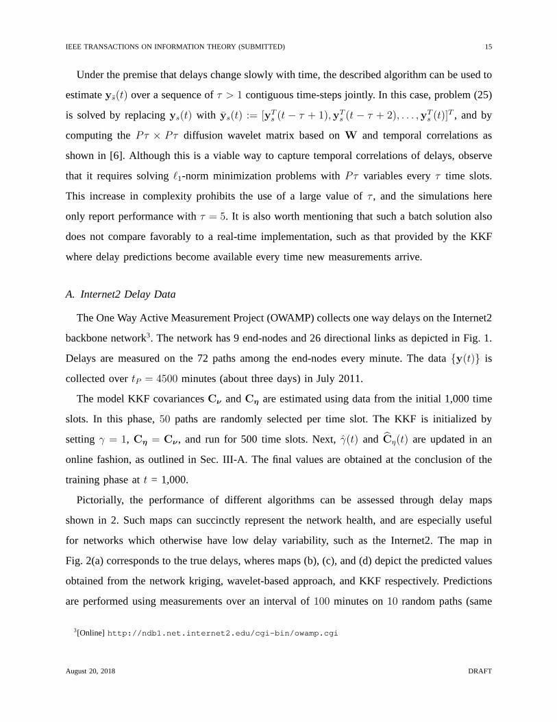
Under the premise that delays change slowly with time, the described algorithm can be used to
estimateys(t) over a sequence ofτ > 1 contiguous time-steps jointly. In this case, problem (25)
is solved by replacingys(t) with ys(t) := [yTs (t − τ + 1),yT
s (t − τ + 2), . . . ,yTs (t)]
T , and by
computing thePτ × Pτ diffusion wavelet matrix based onW and temporal correlations as
shown in [6]. Although this is a viable way to capture temporal correlations of delays, observe
that it requires solvingℓ1-norm minimization problems withPτ variables everyτ time slots.
This increase in complexity prohibits the use of a large value of τ , and the simulations here
only report performance withτ = 5. It is also worth mentioning that such a batch solution also
does not compare favorably to a real-time implementation, such as that provided by the KKF
where delay predictions become available every time new measurements arrive.
A. Internet2 Delay Data
The One Way Active Measurement Project (OWAMP) collects oneway delays on the Internet2
backbone network3. The network has 9 end-nodes and 26 directional links as depicted in Fig. 1.
Delays are measured on the 72 paths among the end-nodes everyminute. The data{y(t)} is
collected overtP = 4500 minutes (about three days) in July 2011.
The model KKF covariancesCν andCη are estimated using data from the initial 1,000 time
slots. In this phase,50 paths are randomly selected per time slot. The KKF is initialized by
settingγ = 1, Cη = Cν , and run for 500 time slots. Next,γ(t) and Cη(t) are updated in an
online fashion, as outlined in Sec. III-A. The final values are obtained at the conclusion of the
training phase att = 1,000.
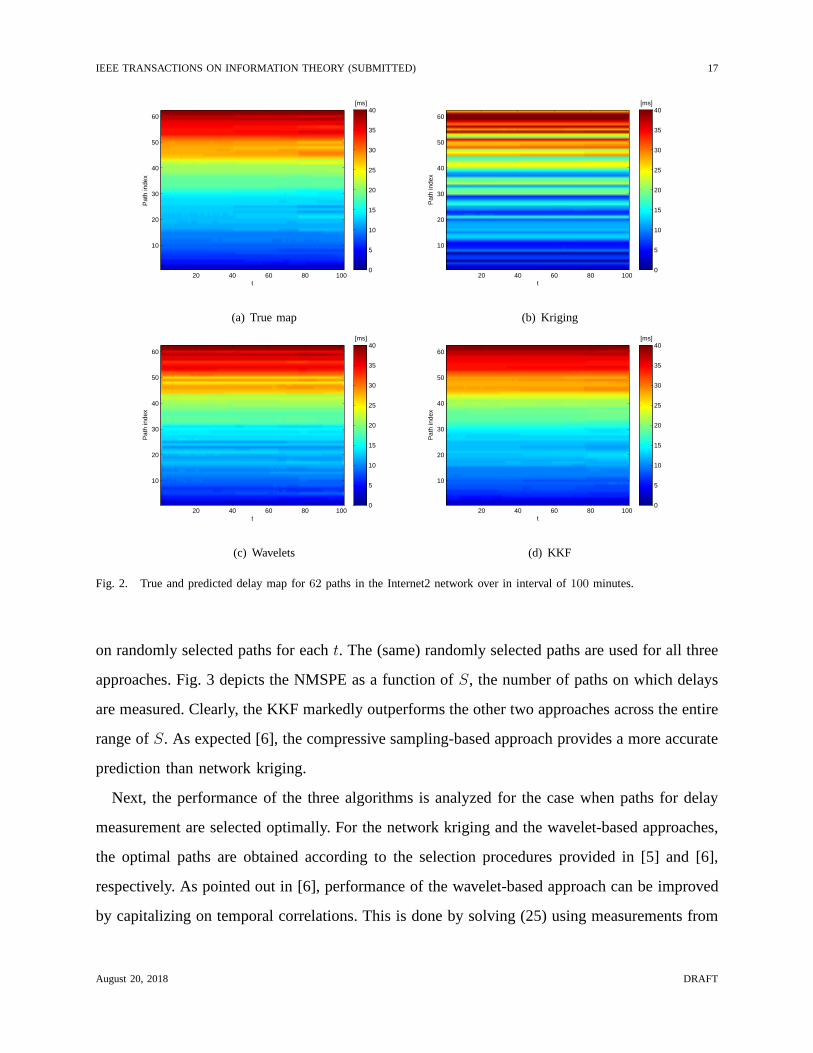
Pictorially, the performance of different algorithms can be assessed through delay maps
shown in 2. Such maps can succinctly represent the network health, and are especially useful
for networks which otherwise have low delay variability, such as the Internet2. The map in
Fig. 2(a) corresponds to the true delays, wheres maps (b), (c), and (d) depict the predicted values
obtained from the network kriging, wavelet-based approach, and KKF respectively. Predictions
are performed using measurements over an interval of100 minutes on10 random paths (same
3[Online] http://ndb1.net.internet2.edu/cgi-bin/owamp.cgi
August 20, 2018 DRAFT

IEEE TRANSACTIONS ON INFORMATION THEORY (SUBMITTED) 16
Fig. 1. Internet2 IP backbone network.
paths are used throughout the considered interval), and thedelays are predicted on the remaining
62 paths are reported. In these maps, paths are arranged in increasing order according to the true
delay at timet = 1. It can be seen that the map produced by the kriging and compressive sensing
approaches are very different from the true map. In contrast, the map obtained when using the
KKF is close to the true map. In particular, observe that the delays of several paths change
slightly aroundt = 80 in Fig. 2(a). However, of the three maps, this change is only discernible
in the KKF map in 2(d). The delay predictions provided by the KKF are thus sufficiently accurate
for human inspection at control centers, even when monitoring a few paths.
It should be remarked that the maps in Fig. 2 are only for demonstration purposes, and not
much can be inferred about the relative performance of different algorithms from these depictions
alone. For a more detailed analysis of the different delay prediction approaches, consider the
normalized mean-square prediction error (NMSPE), defined as
NMSPE:=1
(tP − tL)(P − S)
tP∑
t=tL+1
‖ys(t)− ys(t)‖22 . (26)
The prediction performance of the three algorithms is first assessed by using delay measurements
August 20, 2018 DRAFT
IEEE TRANSACTIONS ON INFORMATION THEORY (SUBMITTED) 17
t
Pat
h in
dex
20 40 60 80 100
10
20
30
40
50
60
0
5
10
15
20
25
30
35
40[ms]
(a) True map
t
Pat
h in
dex
20 40 60 80 100
10
20
30
40
50
60
0
5
10
15
20
25
30
35
40[ms]
(b) Kriging
t
Pat
h in
dex
20 40 60 80 100
10
20
30
40
50
60
0
5
10
15
20
25
30
35
40[ms]
(c) Wavelets
t
Pat
h in
dex
20 40 60 80 100
10
20
30
40
50
60
0
5
10
15
20
25
30
35
40[ms]
(d) KKF
Fig. 2. True and predicted delay map for62 paths in the Internet2 network over in interval of100 minutes.
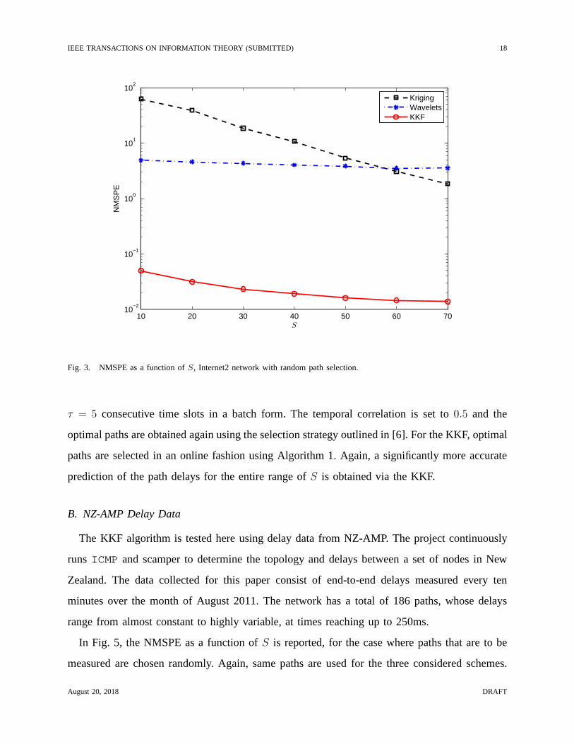
on randomly selected paths for eacht. The (same) randomly selected paths are used for all three
approaches. Fig. 3 depicts the NMSPE as a function ofS, the number of paths on which delays
are measured. Clearly, the KKF markedly outperforms the other two approaches across the entire
range ofS. As expected [6], the compressive sampling-based approachprovides a more accurate
prediction than network kriging.
Next, the performance of the three algorithms is analyzed for the case when paths for delay
measurement are selected optimally. For the network kriging and the wavelet-based approaches,
the optimal paths are obtained according to the selection procedures provided in [5] and [6],
respectively. As pointed out in [6], performance of the wavelet-based approach can be improved
by capitalizing on temporal correlations. This is done by solving (25) using measurements from
August 20, 2018 DRAFT
IEEE TRANSACTIONS ON INFORMATION THEORY (SUBMITTED) 18
10 20 30 40 50 60 7010
−2
10−1
100
101
102
NM
SP
E
S
KrigingWaveletsKKF
Fig. 3. NMSPE as a function ofS, Internet2 network with random path selection.
τ = 5 consecutive time slots in a batch form. The temporal correlation is set to0.5 and the
optimal paths are obtained again using the selection strategy outlined in [6]. For the KKF, optimal
paths are selected in an online fashion using Algorithm 1. Again, a significantly more accurate
prediction of the path delays for the entire range ofS is obtained via the KKF.
B. NZ-AMP Delay Data
The KKF algorithm is tested here using delay data from NZ-AMP. The project continuously
runsICMP and scamper to determine the topology and delays between a set of nodes in New
Zealand. The data collected for this paper consist of end-to-end delays measured every ten
minutes over the month of August 2011. The network has a totalof 186 paths, whose delays
range from almost constant to highly variable, at times reaching up to 250ms.
In Fig. 5, the NMSPE as a function ofS is reported, for the case where paths that are to be
measured are chosen randomly. Again, same paths are used forthe three considered schemes.
August 20, 2018 DRAFT

IEEE TRANSACTIONS ON INFORMATION THEORY (SUBMITTED) 19
10 20 30 40 50 60 70
10−2
10−1
100
101
NM
SP
E
S
KrigingWavelets, τ = 1Wavelets, τ = 5KKF
Fig. 4. NMSPE as a function ofS, Internet2 network with optimal path selection.
The KKF provides a markedly lower prediction error also for the NZ-AMP delay data. On the
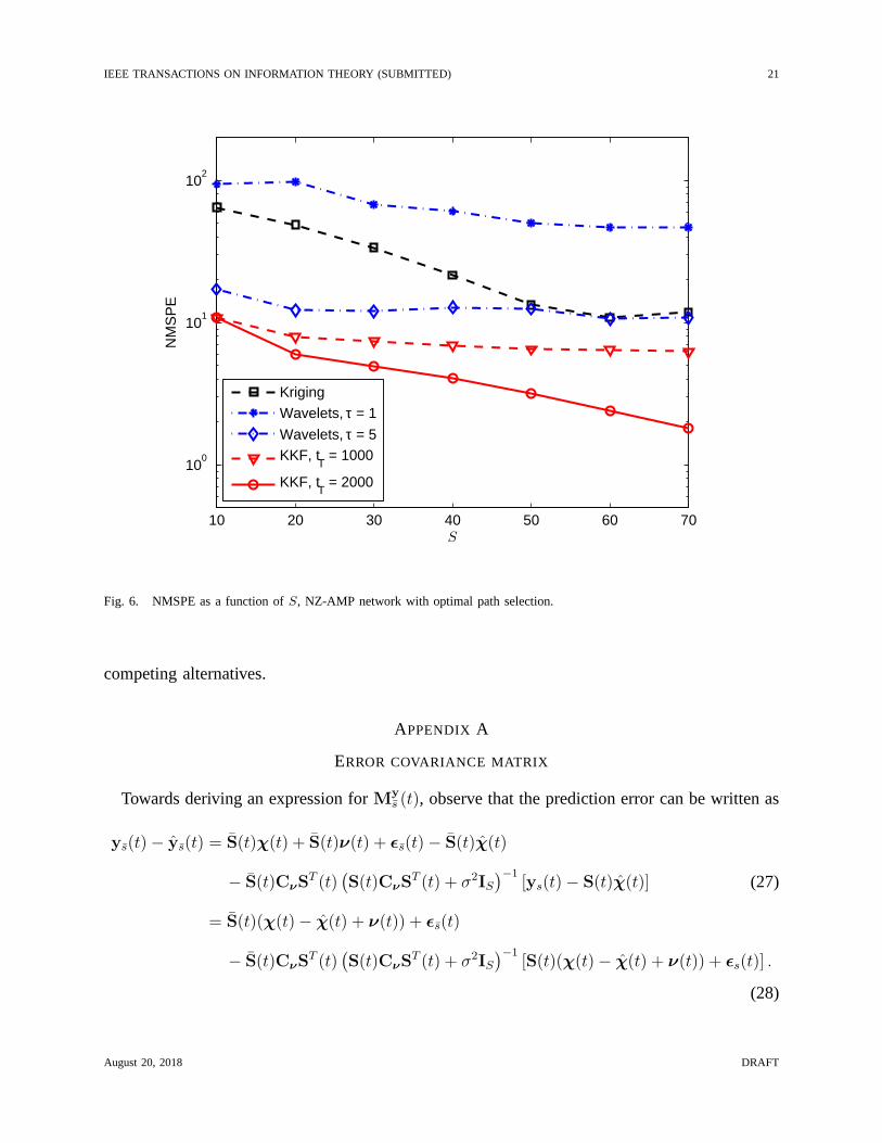
other hand, Fig. 6 shows the NMSPE on optimally selected paths for all three schemes. The
KKF performs relatively better than the competing schemes for this data set as well. Observe
though that the actual values of the NMSPE incurred for this dataset is at least an order of
magnitude higher than those in the Internet2 dataset. Indeed, given the high variability in the
data, it is possible to improve upon the prediction accuracyof KKF by training it better. This is
showcased by the considerably lower prediction error curvefor training intervaltL=2,000 shown
in Fig. 6.
While the NMSPE is useful for characterizing the average performance, network operators
are also interested in the prediction accuracy over the entire range of delay values. Towards
this end, Fig. 7 shows the scatter plots ofys(t) versusys(t) for all t and S = 30 optimally
selected paths. The points cluster around the45-degree lineys(t) = ys(t), and the thinner the
August 20, 2018 DRAFT

IEEE TRANSACTIONS ON INFORMATION THEORY (SUBMITTED) 20
10 20 30 40 50 60 70
101
102
NM
SP
E
S
Kriging
Wavelets
KKF
Fig. 5. NMSPE as a function ofS, NZ-AMP network with random path selection.
“cloud” of points is, the more accurate the estimates are. Indeed, it can be seen that the points
generated from the KKF estimates are crammed in a very close area around the45-degree line,
and accurate estimates are produced for the entire range of experienced delays. Furthermore, the
scatter plots corroborate the unbiasedness of the KKF predictor.
VI. CONCLUSION
The present paper develops a spatio-temporal prediction approach to track and predict network-
wide path delays using measurements on only a few paths. The proposed algorithm adapts a
kriged Kalman filter that exploits both topological as well as historical data. The framework also
allows for the use of submodular optimization in the selection of optimal delay measurement
locations. The problem of path selection is formulated for different types of constraints on the set
of selected paths, and solved in an online fashion to near-optimality. The resulting predictor is
validated on two datasets with different delay profiles, andis shown to substantially outperform
August 20, 2018 DRAFT
IEEE TRANSACTIONS ON INFORMATION THEORY (SUBMITTED) 21
10 20 30 40 50 60 70
100
101
102
NM
SP
E
S
Kriging
Wavelets, τ = 1
Wavelets, τ = 5KKF, t
T = 1000
KKF, tT = 2000
Fig. 6. NMSPE as a function ofS, NZ-AMP network with optimal path selection.
competing alternatives.
APPENDIX A
ERROR COVARIANCE MATRIX
Towards deriving an expression forMys (t), observe that the prediction error can be written as
ys(t)− ys(t) = S(t)χ(t) + S(t)ν(t) + ǫs(t)− S(t)χ(t)
− S(t)CνST (t)
(S(t)CνS
T (t) + σ2IS)−1
[ys(t)− S(t)χ(t)] (27)
= S(t)(χ(t)− χ(t) + ν(t)) + ǫs(t)
− S(t)CνST (t)
(S(t)CνS
T (t) + σ2IS)−1
[S(t)(χ(t)− χ(t) + ν(t)) + ǫs(t)] .
(28)
August 20, 2018 DRAFT

IEEE TRANSACTIONS ON INFORMATION THEORY (SUBMITTED) 22
0 50 100 150 200 250 3000
50
100
150
200
250
300
True delay (ms)
Pre
dic
ted
del
ay(m
s)
(a) Kriging
0 50 100 150 200 250 3000
50
100
150
200
250
300
True delay (ms)
Pre
dic
ted
del
ay(m
s)
(b) Wavelets
0 50 100 150 200 250 3000
50
100
150
200
250
300
True delay (ms)
Pre
dic
ted
del
ay(m
s)
(c) KKF
Fig. 7. Scatter plot for the NZ-AMP network,S = 30 with optimal path selection.
Using (5a), the termχ(t)− χ(t) can be written as
χ(t)− χ(t) = χ(t)− χ(t− 1)−K(t) [S(t)(χ(t) + ν(t)) + ǫs(t)− S(t)χ(t− 1)]
= χ(t)− χ(t− 1) +K(t)S(t)(χ(t)− χ(t− 1) + ν(t)) +K(t)ǫs(t)
= (IP −K(t)S(t))χ(t)−K(t)S(t)ν(t)−K(t)ǫs(t) (29)
whereχ(t) := χ(t)− χ(t− 1). Substituting (29) in (28), it follows that
ys(t)− ys(t) = S(t)(IP −K(t)S(t))(χ(t) + ν(t))− S(t)K(t)ǫs(t) + ǫs(t)
August 20, 2018 DRAFT

IEEE TRANSACTIONS ON INFORMATION THEORY (SUBMITTED) 23
− S(t)CνST (t)
(S(t)CνS
T (t) + σ2IS)−1
× [S(t)(IP −K(t)S(t))(χ(t) + ν(t))− S(t)K(t)ǫs(t) + ǫs(t)] (30)
= S(t)(IP −K(t)S(t))(χ(t) + ν(t))
− S(t)CνST (t)
(S(t)CνS
T (t) + σ2IS)−1
S(t)(IP −K(t)S(t))(χ(t) + ν(t))
− S(t)K(t)ǫs(t)− S(t)CνST (t)
(S(t)CνS
T (t) + σ2IS)−1
(IS − S(t)K(t))ǫs(t)
+ ǫs(t) (31)
which, after some manipulations, can be expressed as
ys(t)− ys(t) = S(t)(IP −Q(t)S(t))(χ(t) + ν(t)) +Q(t)ǫs(t) + ǫs(t) (32)
where
Q(t) := K(t) +CνS(t)(S(t)CνST (t) + σ2IS)
−1 −CνS(t)(S(t)CνST (t) + σ2IS)
−1S(t)K(t).
(33)
Next, substituting forK(t) from (6), the expression forQ(t) simplifies to
Q(t) = (M(t− 1) +Cη)ST (t)
[S(t)(M(t− 1) +Cη +Cν)S
T (t) + σ2IS]−1
+CνST (t)(S(t)CνS
T (t) + σ2IS)−1
−CνST (t)(S(t)CνS
T (t) + σ2IS)−1S(t)(M(t− 1) +Cη)S
T (t)
×[S(t)(M(t− 1) +Cη +Cν)S
T (t) + σ2IS]−1
(34)
= (M(t− 1) +Cη +Cν)ST (t)
[S(t)(M(t− 1) +Cη +Cν)S
T (t) + σ2IS]−1
. (35)
Utilizing the fact thatχ(t), ν(t), ǫs(t), andǫs(t) are mutually uncorrelated, withE[χ(t)χT (t)
]:=
M(t− 1) +Cη, the error covariance matrixMys (t) becomes
Mys (t) = E
[(ys(t)− ys(t))(ys(t)− ys(t))
T]
(36)
= S(t)(IP −Q(t)S(t))(M(t− 1) +Cν +Cη)(IP − ST (t)QT (t))ST (t)
+ σ2S(t)Q(t)QT (t)ST (t) + σ2IP−S (37)
= S(t)(M(t− 1) +Cν +Cη)ST (t)− 2S(t)Q(t)S(t)(M(t− 1) +Cν +Cη)S
T (t)
August 20, 2018 DRAFT

IEEE TRANSACTIONS ON INFORMATION THEORY (SUBMITTED) 24
+ S(t)Q(t)S(t)(M(t− 1) +Cη +Cν)ST (t)QT (t)ST (t) + σ2S(t)Q(t)QT (t)ST (t)
+ σ2IP−S (38)
= S(t)(M(t− 1) +Cν +Cη)ST (t)− S(t)Q(t)S(t)(M(t− 1) +Cν +Cη)S
T (t)
+ σ2IP−S. (39)
Substituting forQ(t) [cf. (35)] in (39), and using the Woodbury matrix identity [32], the final
expression forMys (t) becomes
Mys (t) = σ2IP−S + S(t)
[(M(t− 1) +Cν +Cη
)−1+
1
σ2ST (t)S(t)
]−1
ST (t) . (40)
APPENDIX B
PROOF OF MONOTONICITY AND SUPERMODULARITY OFf
Let Φ := 1σ2 (M(t− 1) +Cη +Cν), and observe thatf can be written as
f(S) = log(σ2) + log det[IP−S + S(Φ−1 + STS)−1ST
](41a)
= log(σ2) + log det[IP + ST S(Φ−1 + STS)−1
](41b)
= log(σ2) + log det[Φ−1 + STS+ ST S
]+ log det
[(Φ−1 + STS)−1
](41c)
where (41b) follows from Sylvester’s theorem for determinants [32].
Observing thatST S+ STS = IP , it is possible to writef(S) as
f(S) = log(σ2) + log det(Φ−1 + IP )− log det(Φ−1 + STS
). (42)
Next, consider the decompositionΦ = UUT , and define the shifted function
h(S) := f(S)− log(σ2)− log det (Φ+ IP ) (43a)
= − log det(IP + STSΦ) (43b)
= − log det[IS + (SU)(SU)T
](43c)
where Sylvester’s theorem has again been used in (43c). Finally, it is well known that a function
of the form log det(IP +(SU)T (SU)) is non-decreasing and submodular (see e.g., [25]), which
allows one to deduce thatf(S) is non-increasing and supermodular. Note further that the greedy
approach from [27] can be used onh(S) by definingh(∅) = 0.
August 20, 2018 DRAFT

IEEE TRANSACTIONS ON INFORMATION THEORY (SUBMITTED) 25
REFERENCES
[1] H. Singhal and G. Michailidis, “Structural models for dual modality data with application to network tomography,”IEEE
Trans. Inf. Theory, vol. 57, no. 8, pp. 5054–5071, Aug. 2011.
[2] M. G. Rabbat, M. A. T. Figueiredo, and R. D. Nowak, “Network inference from co-occurrences,”IEEE Trans. Inf. Theory,
vol. 54, no. 9, pp. 4053–4068, Sep. 2008.
[3] B. D. Ripley, Spatial Statistics. John Wiley & Sons, 1981.
[4] N. Cressie, “The origins of kriging,”Mathematical Geology, vol. 22, no. 3, pp. 239–252, 1990.
[5] D. B. Chua, E. D. Kolaczyk, and M. Crovella, “Network kriging,” IEEE J. Sel. Areas Commun., vol. 24, no. 12, pp.
2263–2272, Dec. 2006.
[6] M. Coates, Y. Pointurier, and M. Rabbat, “Compressed network monitoring for IP and all-optical networks,” inProc. ACM
Internet Measurement Conf., San Diego, CA, Oct. 2007.
[7] W. Xu, E. Mallada, and A. Tang, “Compressive sensing overgraphs,” inProc. of IEEE INFOCOM, Shanghai, China, Apr.
2011, pp. 2087–2095.
[8] F. Dabek, R. Cox, F. Kaashoek, and R. Morris, “Vivaldi: A decentralized network coordinate system,” inProc. of the ACM
SIGCOMM, Portland, Oregon, USA, 2004, pp. 15–26.
[9] Y. Liao, P. Geurts, and G. Leduc, “Network distance prediction based on decentralized matrix factorization,” inProc. of
IFIP Networking, Chennai, India, May 2010.
[10] A. Lakhina, K. Papagiannaki, M. Crovella, C. Diot, E. D.Kolaczyk, and N. Taft, “Structural analysis of network traffic
flows,” in Proc. of ACM SIGMETRICS, New York, NY, 2004, pp. 61–72.
[11] C. J. Bovy, H. T. Mertodimedjo, G. Hooghiemstra, H. Uijterwaal, and P. van Mieghem, “Analysis of end-to-end delay
measurements in Internet,” inProc. Passive and Active Measurement Workshop, Fort Collins, CO, Apr. 2002.
[12] K. V. Mardia, C. Goodall, E. J. Redfern, and F. J. Alonso,“The Kriged Kalman filter,”Test, vol. 7, no. 2, pp. 217–285,
Dec. 1998.
[13] C. K. Wikle and N. Cressie, “A dimension-reduced approach to space-time Kalman filtering,”Biometrika, vol. 86, no. 4,
pp. 815–829, 1999.
[14] S.-J. Kim, E. Dall’Anese, and G. B. Giannakis, “Cooperative spectrum sensing for cognitive radios using Kriged Kalman
filtering,” IEEE J. Sel. Topics Signal Process., vol. 5, no. 1, pp. 24–36, Feb. 2011.
[15] J. Cortes, “Distributed Kriged Kalman filter for spatial estimation,”IEEE Trans. Auto. Contr., vol. 54, no. 12, pp. 2816–
2827, Dec. 2009.
[16] B. D. O. Anderson and J. B. Moore,Optimal Filtering. Englewood Cliffs, NJ: Prentice-Hall, 1979.
[17] P. Casas, S. Vaton, L. Fillatre, and T. Chonavel, “Efficient methods for traffic matrix modeling and on-line estimation in
large-scale ip networks,” inProc. of the 21st Intl. Teletraffic Congress, Paris, France, 2009, pp. 45–54.
[18] E. Dall’Anese, S.-J. Kim, and G. Giannakis, “Channel gain map tracking via distributed kriging,”IEEE Trans. Veh. Technol.,
vol. 60, no. 3, pp. 1205–1211, Mar. 2011.
[19] I. D. Schizas, A. Ribeiro, and G. B. Giannakis, “Consensus in ad hoc WSNs with noisy links - part I: Distributed estimation
of deterministic signals,”IEEE Trans. Signal Process., vol. 56, no. 1, pp. 350–364, Jan. 2008.
August 20, 2018 DRAFT

IEEE TRANSACTIONS ON INFORMATION THEORY (SUBMITTED) 26
[20] R. Mehra, “On the identification of variances and adaptive Kalman filtering,”IEEE Trans. Autom. Control, vol. 15, no. 2,
pp. 175–184, Apr. 1970.
[21] K. Myers and B. Tapley, “Adaptive sequential estimation with unknown noise statistics,”IEEE Trans. Autom. Control,
vol. 21, no. 4, pp. 520–523, Aug. 1976.
[22] M. K. Tsatsanis and G. B. Giannakis, “Modeling and equalization of rapidly fading channels,”Intl. J. Adaptive Control
and Signal Process., vol. 10, no. 2-3, pp. 159–176, 1996.
[23] M. K. Tsatsanis, G. B. Giannakis, and G. Zhou, “Modelingand equalization of rapidly fading channels,”Signal Process.,
vol. 53, no. 2-3, pp. 211–229, 1996.
[24] C. M. Bishop,Pattern Recognition and Machine Learning. Springer, New York, 2006.
[25] F. Bach, “Learning with submodular functions: A convexoptimization perspective,”Foundations and Trends in Machine
Learning, 2012. [Online]. Available: http://arxiv.org/abs/1111.6453
[26] A. Das and D. Kempe, “Algorithms for subset selection inlinear regression,” inProc. of the ACM Symp. on Theory of
Computing, Victoria, British Columbia, Canada, May 2008, pp. 45–54.
[27] G. L. Nemhauser, L. A. Wolsey, and M. L. Fisher, “An analysis of approximations for maximizing submodular set functions
- I,” Mathematical Programming, no. 1, pp. 265–294, Dec. 1978.
[28] M. Minoux, “Accelerated greedy algorithms for maximizing submodular set functions,” inOptimization Techniques, ser.
Lecture Notes in Control and Information Sciences, J. Stoer, Ed. Springer Berlin / Heidelberg, 1978, vol. 7, pp. 234–243.
[29] M. L. Fisher, G. L. Nemhauser, and L. A. Wolsey, “An analysis of approximations for maximizing submodular set functions
- II,” Mathematical Programming Study, pp. 73–87, 1978.
[30] R. R. Coifman and M. Maggioni, “Diffusion wavelets,”Applied and Computational Harmonic Analysis, vol. 21, no. 1,
pp. 53–94, 2006.
[31] R. Sinkhorn, “A relationship between arbitrary positive matrices and doubly stochastic matrices,”The Annals of
Mathematical Statistics, vol. 35, no. 2, pp. 876–879, 1964.
[32] G. H. Golub and C. F. V. Loan,Matrix Computations, 3rd ed. Johns Hopkins University Press, 1996.
August 20, 2018 DRAFT
Related Documents


