Idiosyncratic Risk, Market Risk and Correlation Dynamics in European Equity Markets

IIIS Discussion Paper

No.15 / January 2004

Idiosyncratic Risk, Market Risk and CorrelationDynamics in European Equity Markets

Colm Kearney and Valerio PotìTrinity College Dublin

IIIS Discussion Paper No. 15

Idiosyncratic Risk, Market Risk and Correlation Dynamics in European Equity Markets Colm Kearney and Valerio Potì,

Disclaimer Any opinions expressed here are those of the author(s) and not those of the IIIS. All works posted here are owned and copyrighted by the author(s). Papers may only be downloaded for personal use only.

Idiosyncratic Risk, Market Risk and Correlation Dynamics in European Equity Markets

Colm Kearney and Valerio Potì, School of Business Studies,

Trinity College, Dublin.

June 2003

Abstract

We examine total, market and idiosyncratic risk and correlation dynamics using daily data from 1993 to 2001 on the 6 largest euro-zone stock market indices and 42 firms from the Dow Jones Eurostoxx50 index. We also estimate conditional correlations using the asymmetric DCC-MVGARCH model. Comparing our results with those of Campbell, Lettau, Malkiel and Xu (2001), stock correlations are higher and have declined less in the euro-zone than in the United States over the 1990s, implying a lower benefit from diversification strategies. By contrast, correlations amongst market indices have risen, with a structural break related to the process of financial integration in the euro-zone.

Key Words: Correlation dynamics, GARCH, idiosyncratic risk. JEL Classification: C32, G12, G15.

Contact details: Colm Kearney, Professor of International Business, Government of Ireland Senior Research Fellow, School of Business Studies, Trinity College, Dublin 2, Ireland. Tel: 3531-6082688, Fax: 3531- 6799503. Email: [email protected]. Valerio Potì, Government of Ireland Research Scholar, School of Business Studies, Trinity College, Dublin 2, Ireland. Tel: 3531-6082017, Fax: 3531- 6799503. Email: [email protected]. Previous versions of this paper were presented at the European meeting of the Financial Management Association in Dublin, June 2003 and at the Annual Meeting of the European Finance Association in Glasgow, August 2003. Both authors acknowledge financial support from the Irish Research Council for the Humanities and the Social Sciences.

1

Idiosyncratic Risk, Market Risk and Correlation Dynamics in European Equity Markets

1. Introduction.

International fund managers usually divide their equity portfolios into a number

of regions and countries, and select stocks in each country with a view to

outperforming an agreed market index by some percentage. This provides asset

diversity within each country together with international diversification across

political frontiers. Two interrelated features of this strategy have attracted the

recent attention of financial researchers and practitioners. The first relates to

expected returns. A growing body of empirical evidence on the performance of

mutual and pension fund managers has questioned the extent to which they

systematically outperform their benchmarks (Blake and Timmerman, 1998,

Wermers, 2000, Baks, Metrick and Wachter, 2001, and Coval and Moskowitz,

2001). To the extent that fund managers fail to add value when account is taken

of their fees, the more passive strategy of buying and holding the market index

for each country might yield an equally effective but more cost-efficient

international diversification. The second relates to risk. It has been known for

some time that equity return correlations do not remain constant over time,

tending to decline in bull markets and to rise in bear markets (De Santis and

Gerard (1997), Ang and Bekaert (1999), and Longin and Solnik (2003)).

Correlations also tend to rise with the degree of international equity market

integration (Erb, Harvey and Viskanta (1994) and Longin and Solnik (1995)),

which has gathered pace in Europe since the mid-1990s (Hardouvelis,

Malliaropulos and Priestley (2000) and Fratzschler (2002))1. It is of

considerable interest, therefore, to investigate the relative strengths of the trends

in variances and correlations at the firm level as well as at the market index level

in European equity markets, because the findings have relevance for the

diversification properties of passive and active international investment

strategies.

1 The latter author also notes that the euro-zone equity market has now surpassed the United States markets as the most influential determinant of euro-zone country equity returns.

2

In this paper, we investigate the trends in firm-level and market index

correlations in European equity markets using over 2,300 daily observations

from January 1993 to November 2001 on 42 stocks from the Dow Jones

Eurostoxx50. We analyse the behaviour over time of market risk and aggregate

idiosyncratic risk in a portfolio of these stocks. We also study the pattern of

aggregate correlation between the indexes of the 5 largest euro-zone stock

markets and the Eurostoxx50 index. We extend the variance decomposition

methodology of Campbell, Lettau, Malkiel and Xu (2001), (henceforth CLMX

(2001)) to provide a full description of the relation between changes in market

risk, aggregate idiosyncratic risk and return correlations. We then apply the

recently developed dynamic conditional correlation multivariate generalised

autoregressive conditional heteroscedasticity (DCC-MVGARCH) model of

Engle (2001) and Engle and Sheppard (2002) to capture the time series

behaviour of the conditional correlations between the leading euro-zone market

indexes and between the individual stocks in the Eurostoxx50 index. In doing

so, we specify our model to facilitate testing for non-stationarity and

asymmetries in the correlation processes.

We find that, consistently with the results reported by CLMX (2001) for the

United States, average firm-level variance has trended upwards in the euro-zone

area. Contrary to CLMX (2001), however, we find that market variance has also

trended upwards, but by less than the rise in firm-level variance. This implies

the existence of different correlation dynamics in the euro-zone area during the

past 10 years to those observed in the United States, with a smaller downward

trend in average correlation in our sample of euro-zone stocks. We also find

significant persistence in all our conditional volatilities and correlation estimates,

with the dynamics of firm-level correlations being best explained by an

asymmetric component in their processes. Stock correlations tend to spike up

after negative return innovations, suggesting that diversification strategies might

perform poorly during prolonged bear markets. Finally, we find a significant

rise in the correlations amongst euro-zone market indexes that can best be

explained by a structural break reflecting the process of monetary and financial

3

integration in Europe. It follows that portfolio managers in Europe should not

over-estimate the benefits of pursuing passive international diversification

strategies based on holding national stock market indexes. This conclusion is

strengthened by the fact that correlations amongst the individual stocks in the

euro-zone area have not been pushed upwards by the integration process, so firm

level diversification strategies retain their appeal.

Our paper is structured as follows. We begin by generalising the CLMX (2001)

decomposition of variance to provide a more complete description of the relation

between market risk, aggregate idiosyncratic risk and correlation dynamics. In

Section 3, we describe our data set, provide summary statistics, and present the

salient trends in firm-level and market correlations in the euro-zone area. In

Section 4, we perform a range of statistical tests to discern more formally the

behaviour of market risk, firm-level risk and correlations in our dataset. We

implement unit root and Wald tests, and we apply the DCC-MVGARCH model

to our data. In the final Section, we summarise our main findings and draw

together our conclusions.

2. Idiosyncratic Risk, Market Risk and Average Correlation.

The simplified market model can be written as an empirical version of the

Sharpe (1964) and Lintner (1965) security market line.

titmtitmiti rrr ,,,,, ηεβ +=+= (1)

Here, tir , is the excess return on asset i at time t, tmr , is the excess return on the

market portfolio, iβ is the asset’s beta coefficient, ti,ε is the usual CAPM

idiosyncratic residual, and ti ,η is the market-adjusted excess return on asset i

computed according to the simplified market model. Letting tiw , denote the

weight of asset i in the market portfolio, we can compute the weighted average

of the variance of returns on the n stocks in the market portfolio.

4

� ��= ==

++=n

i

n

ititmtitititm

n

ititi rCovwVarwrVarrVarw

1 1,,,,,,

1,, ),(2)()()( ηη (2)

By substituting for ti ,η from (1), noting that tmr , and ti ,ε are orthogonal, and

recalling that the weighed average of the iβ coefficients is equal to 1, the last

term on the right collapses to zero, and we are left with the CLMX (2001)

variance decomposition:

)( ,1

, ti

n

itit rVarwVAR �

=

=

� �= =

−++=n

i

n

itmititititm rVarwVarwrVar

1 1,,,,, )()1(2)()( βη

�=

+=n

itititm VarwrVar

1,,, )()( η

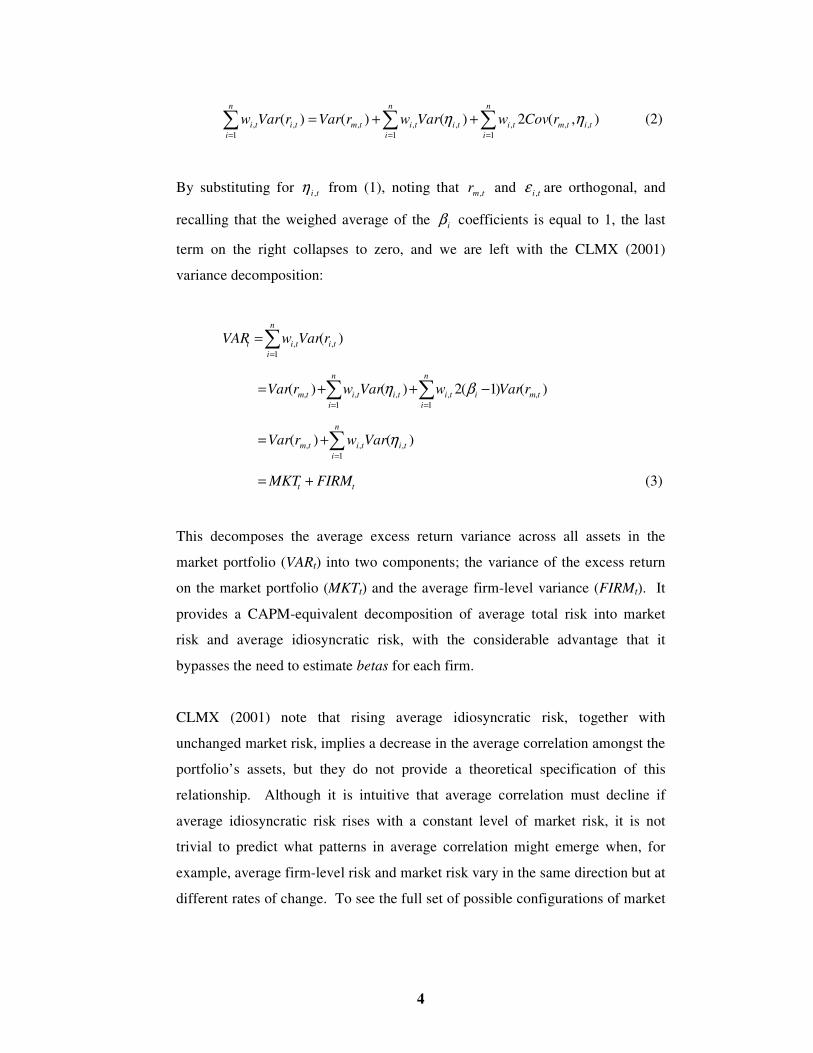
tt FIRMMKT += (3)

This decomposes the average excess return variance across all assets in the

market portfolio (VARt) into two components; the variance of the excess return

on the market portfolio (MKTt) and the average firm-level variance (FIRMt). It

provides a CAPM-equivalent decomposition of average total risk into market

risk and average idiosyncratic risk, with the considerable advantage that it

bypasses the need to estimate betas for each firm.

CLMX (2001) note that rising average idiosyncratic risk, together with

unchanged market risk, implies a decrease in the average correlation amongst the

portfolio’s assets, but they do not provide a theoretical specification of this

relationship. Although it is intuitive that average correlation must decline if

average idiosyncratic risk rises with a constant level of market risk, it is not

trivial to predict what patterns in average correlation might emerge when, for

example, average firm-level risk and market risk vary in the same direction but at

different rates of change. To see the full set of possible configurations of market

5

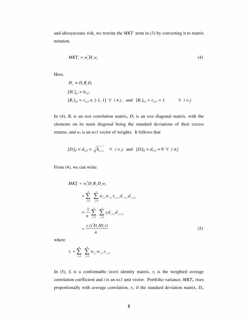
and idiosyncratic risk, we rewrite the MKT term in (3) by converting it to matrix

notation.

tttt wHwMKT ′= (4)

Here,

tttt DRDH ≡

[Ht ]i,j = hi,j,t

[Rt ]i,j = ri,j,t ∈ [-1, 1] ∀ i ≠ j , and [Rt ]i,j = ri,j,t = 1 ∀ i = j

In (4), Rt is an nxn correlation matrix, Dt is an nxn diagonal matrix, with the

elements on its main diagonal being the standard deviations of their excess

returns, and wt is an nx1 vector of weights. It follows that

[Dt]ij = di,j,t = tjih ,, ∀ i = j, and [Dt]ij = di,j,t = 0 ∀ i ≠ j

From (4), we can write:

tMKT ttttt wDRDw′=

��==

=n

jtjitjitjitjti

n

i

ddrww1

,,,,,,,,1

��==

=n

jtjjtiit

n

i

ddrn 1

,,,,1

1

n

iIDDir ttt )( ′= (5)

where

��==

=n

jtjitjti

n

it rwwr

1,,,,

1

In (5), It is a conformable (nxn) identity matrix, rt is the weighted average

correlation coefficient and i is an nx1 unit vector. Portfolio variance, MKTt, rises

proportionally with average correlation, rt, if the standard deviation matrix, Dt,

6

remains constant. Using (5), we can rewrite (3) for the variance decomposition

as in (6).

VARt = n

)iIDDi(r ttt ′ + FIRMt (6)

Solving (6) for rt, the average correlation coefficient becomes

���

����

�

′−

′′

=iDDi

FIRMiDDiiDDw

nrtt

t

tt

tttt (7)

and for equally-weighted portfolios with wt = n1

i, it can be rewritten as

���

����

�

′−

′′

=iDDi

FIRMiDDiiDDi

nnr

tt

t

tt

tttt

1

niDDi

FIRM

tt

t

/)(1

′−=

t

t

VARFIRM

−= 1 = t

tt

VARFIRMVAR −

= t

t

VARMKT

(8)

Equation (8) provides an intuitively appealing result. Average correlation is the

the ratio between market risk and average idiosyncratic risk. Moreover, we can

rewrite (8) as,

tttt FIRMVARrVAR +=

tt FIRMMKT += (9)

7

Equation (9) tells us that, at least for an equally weighted market portfolio, we

can interpret average correlation as the parameter that, for any given level of

average total risk, divides the latter into market risk and idiosyncratic risk. By

differentiating rt in (8) with respect to the ratio of average idiosyncratic variance

to average total variance, we obtain

)VAR/FIRM(d

dr

tt

t = -1 (10)

This holds exactly in the equally weighted case, but it holds approximately in

general, so we write it as

)VAR/FIRM(d

dr

tt

t ≅ -1 (11)

Equations (10) and (11) show that the variation in average correlation is

inversely proportional to the variation in the ratio of average firm-level variance

to market variance. The larger the number of stocks included in a portfolio, the

more it resembles an equally-weighted portfolio and the better is the

approximation provided by (10). Average correlation is strongly influenced by

the extent to which firms diversify internally. The more the average firm

diversifies (the more it resembles the market portfolio), the higher will be the

average correlation for each given level of covariance risk in the economy

(MKTt). The opposite is true for average firm-level variance.

3. Data, Summary Statistics and Trends

Our dataset comes from two sources. The firm-level data is drawn from the

stocks included in the Eurostoxx50 index. This is the leading European stock

market index, and the futures contract on this index is one of the most liquid in

the world. It commenced on 31 December 1991 with a base value of 1000, and

it comprises 50 stocks from the companies with the heaviest capitalisation in the

8

euro-zone countries2. We use the Bloomberg database of daily closing prices on

the constituent stocks of the index to derive daily returns for the individual

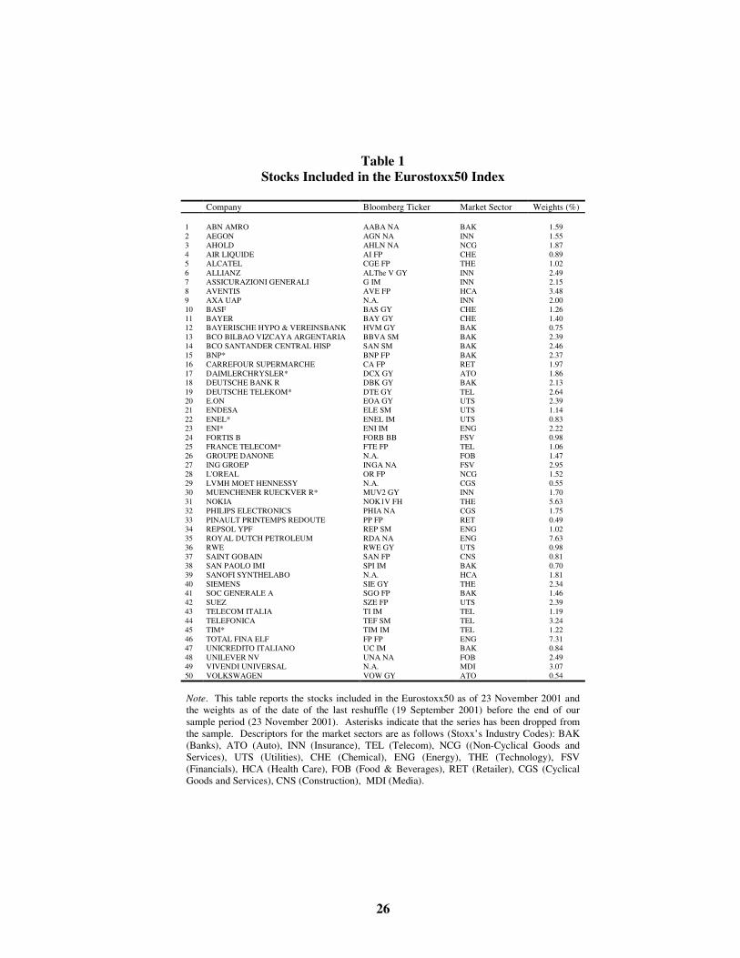
stocks. Table 1 lists the stocks included in the Eurostoxx50 index at the end of

our sample period along with their weights at the date of the last reshuffle (19

September 2001). We select all 42 stocks with a continuous returns series from

February 1993 to November 20013. It is noteworthy that our sample of euro-

zone firm-level data comprising the largest stocks in the Eurostoxx50 index

differs from that employed by CLMX (2001), which includes large, medium and

small United States stocks. Table 2 provides the usual set of summary statistics

for the 42 individual stock returns, and for the returns on the 6 market indices.

In particular, we report the sample means, variances, skewness, kurtosis, the

Jarque-Bera statistics and their associated significance levels. As expected, the

returns exhibit significant departure from the normal distribution in most cases.

Setting n = 42, we define market variance (MKTt) over a 21-day month (T = 21)

as the sum of the squared deviations of daily market returns (Rm,t) from their

sample mean4, ( mR ).

�=

−=T

tmtmt RRMKT

1

2, )( with �

=

=n

it,it,it,m RwR

1 (12)

Here, Ri,t is the return on stock i at time t. To construct the average total variance

series, VARt, we first compute the monthly variance for each stock in our sample,

VAR(Ri,t) as the sum of the squared deviations of their daily returns from their

sample mean, iR .

�=

−=T

tititi RRRVar

1

2,, )()( (13)

2 Stoxx (part of the Dow Jones Telerate Group) publishes various indexes. Among these, a version of the Dow Jones Eurostoxx50 index that includes the UK stock market is also available. 3 The excluded stocks are also listed in Table 1 and indicated by ‘*’s. 4 As in CLMX (2001) we experimented also with time-varying means, but the results are almost identical.

9

We then average across the variances of all stocks in our sample to compute the

average total variance as

�=

=n

it,it,it )R(VarwVAR

1 (14)

Finally, using (3) we compute the average firm-level variance as the difference

between VARt and MKTt:

ttt MKTVARFIRM −= (15)

The market variance time series (MKTt) defined by (12), the average total

variance (VARt) defined by (14), and the average firm-level variance (FIRMt)

defined by (15) each contain 103 monthly observations for the period 1993 -

2001. The stock weights are equal to n1 (n = 42) in the equally-weighted case,

and to the ratio of the capitalisation of each stock to the capitalisation of the

market portfolio in the value-weighted case. Our resulting series are therefore

equally-weighted and value-weighted averages of market, firm-level, and total

risk.

In Figure 1, we plot the time series of market variance (MKTt), average firm-

level variance (FIRMt), and average total variance (VARt) for the equally-

weighted (Panel A) and for the value-weighted (Panel B) cases. It is noticeable

that the equally-weighted and value-weighted series behave very similarly.

Indeed, their behaviour turns out to be almost identical in all our subsequent

tests, and we consequently report only the results for the equally-weighted case.

Both the firm-level and the market variances start off relatively low and tend to

rise towards the end of the period. This tendency is more pronounced for the

firm-level variance than for the market variance. In this respect, our data appears

to behave similarly to CMLX (2001) who note that average firm-level variance

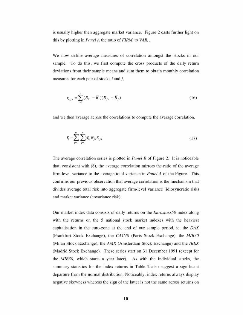
10

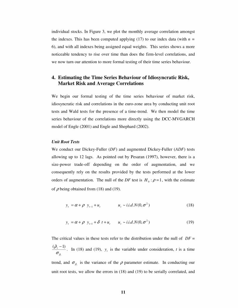
is usually higher then aggregate market variance. Figure 2 casts further light on

this by plotting in Panel A the ratio of FIRMt to VARt .

We now define average measures of correlation amongst the stocks in our

sample. To do this, we first compute the cross products of the daily return

deviations from their sample means and sum them to obtain monthly correlation

measures for each pair of stocks i and j,

)()( ,1

,,, jtj

T

tititji RRRRr −−=�

= (16)

and we then average across the correlations to compute the average correlation.

��==

=n

jt,j,it,jt,i

n

it rwwr

11 (17)

The average correlation series is plotted in Panel B of Figure 2. It is noticeable

that, consistent with (8), the average correlation mirrors the ratio of the average

firm-level variance to the average total variance in Panel A of the Figure. This

confirms our previous observation that average correlation is the mechanism that

divides average total risk into aggregate firm-level variance (idiosyncratic risk)

and market variance (covariance risk).

Our market index data consists of daily returns on the Eurostoxx50 index along

with the returns on the 5 national stock market indexes with the heaviest

capitalisation in the euro-zone at the end of our sample period, ie, the DAX

(Frankfurt Stock Exchange), the CAC40 (Paris Stock Exchange), the MIB30

(Milan Stock Exchange), the AMX (Amsterdam Stock Exchange) and the IBEX

(Madrid Stock Exchange). These series start on 31 December 1991 (except for

the MIB30, which starts a year later). As with the individual stocks, the

summary statistics for the index returns in Table 2 also suggest a significant

departure from the normal distribution. Noticeably, index returns always display

negative skewness whereas the sign of the latter is not the same across returns on

11

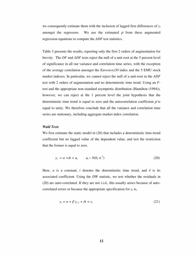
individual stocks. In Figure 3, we plot the monthly average correlation amongst

the indexes. This has been computed applying (17) to our index data (with n =

6), and with all indexes being assigned equal weights. This series shows a more

noticeable tendency to rise over time than does the firm-level correlations, and

we now turn our attention to more formal testing of their time series behaviour.

4. Estimating the Time Series Behaviour of Idiosyncratic Risk, Market Risk and Average Correlations

We begin our formal testing of the time series behaviour of market risk,

idiosyncratic risk and correlations in the euro-zone area by conducting unit root

tests and Wald tests for the presence of a time-trend. We then model the time

series behaviour of the correlations more directly using the DCC-MVGARCH

model of Engle (2001) and Engle and Shephard (2002).

Unit Root Tests

We conduct our Dickey-Fuller (DF) and augmented Dickey-Fuller (ADF) tests

allowing up to 12 lags. As pointed out by Pesaran (1997), however, there is a

size-power trade-off depending on the order of augmentation, and we

consequently rely on the results provided by the tests performed at the lower

orders of augmentation. The null of the DF test is 1:0 =ρH , with the estimate

of ρ being obtained from (18) and (19).

ttt uyy ++= −1ρα ),0(...~ 2σNdiiu t (18)

ttt utyy +++= − δρα 1 ),0(...~ 2σNdiiu t (19)

The critical values in these tests refer to the distribution under the null of DF =

t

t

ρσρ

ˆ

)1ˆ( −. In (18) and (19), ty is the variable under consideration, t is a time

trend, and tρσ ˆ is the variance of the ρ parameter estimate. In conducting our

unit root tests, we allow the errors in (18) and (19) to be serially correlated, and

12

we consequently estimate them with the inclusion of lagged first differences of yt

amongst the regressors. We use the estimated ρ from these augmented

regression equations to compute the ADF test statistics.

Table 3 presents the results, reporting only the first 2 orders of augmentation for

brevity. The DF and ADF tests reject the null of a unit root at the 5 percent level

of significance in all our variance and correlation time series, with the exception

of the average correlation amongst the Eurostoxx50 index and the 5 EMU stock

market indexes. In particular, we cannot reject the null of a unit-root in the ADF

test with 2 orders of augmentation and no deterministic time trend. Using an F-

test and the appropriate non-standard asymptotic distribution (Hamilton (1994)),

however, we can reject at the 1 percent level the joint hypothesis that the

deterministic time trend is equal to zero and the autocorrelation coefficient ρ is

equal to unity. We therefore conclude that all the variance and correlation time

series are stationary, including aggregate market index correlation.

Wald Tests

We first estimate the static model in (20) that includes a deterministic time-trend

coefficient but no lagged value of the dependent value, and test the restriction

that the former is equal to zero.

yt = � +�t + ut ut ~ N(0, � 2) (20)

Here, � is a constant, t denotes the deterministic time trend, and � is its

associated coefficient. Using the DW statistic, we test whether the residuals in

(20) are auto-correlated. If they are not i.i.d., this usually arises because of auto-

correlated errors or because the appropriate specification for yt is,

yt = � + � yt-1 + �t + �t (21)

13

Whenever we detect serial correlation in the residuals of the static model in (20),

we estimate the dynamic model in (21) using Durbin’s h5 statistic to check that

the residuals are serially independent. We conduct a Wald-type test of the

restriction that the deterministic time trend coefficient is zero using Newy-West

adjusted variance-covariance matrices to correct for heteroschedasticity and

autocorrelation. Table 4 presents the results. We can never reject the null that the

residuals from (21) are serially independent, with the exception of the average

firm-level variance (FIRM,t) and of the average correlation amongst the market

indices (rt in the bottom panel of Table 4). In the latter 2 cases, we must

therefore treat the parameter estimates with caution, because inference

procedures are not in general valid due to biased parameter variance estimates

and inconsistent OLS estimates. As far as the relative sizes of the deterministic

time-trend of MKTt and FIRMt are concerned, the coefficient estimated for the

latter is always greater than for the former. Moreover, the deterministic time-

trend coefficient is always positive, except for the average stock returns

correlation series. Not surprisingly, because of the relative size of the

deterministic time trend coefficient of MKTt and FIRMt, average stock

correlation is trended downwards, which is consistent with (10) and (11). One

noticeable feature of average market index correlation is the large positive

estimate of the deterministic time trend coefficient. This confirms that, as

suggested by visual inspection of Figure 3, market correlations in the Euro-zone

have greatly increased over the period 1993-2001.

Summarising our results thus far, both the variance and correlation time series,

based respectively on sums of squares in (13) and sums of cross-products in (16),

appear to be stationary, especially when we allow for a deterministic time trend.

Both aggregate firm-level and market variance have trended upwards in the euro-

zone over the period 1993-2001. Our estimated time trend coefficient for average

idiosyncratic variance is smaller than the equally weighted estimate reported by

5 In the presence of lagged values of the dependent variables the DW test is biased toward acceptance of the null of no error auto-correlation. We therefore test for serial correlation of the error terms using Durbin’s (1970) h-test. We use the generalised version this test, developed by Godfrey and Breusch, based on a general Lagrange Multiplier test. Even though this procedure can detect higher order serial correlation, we only test the null of no first-order residual autocorrelation.

14

CLMX (2001)6 for a large sample of United States stocks. In addition, we do not

find that the average correlation amongst euro-zone stock returns has declined

sharply as reported by CLMX for the United States markets7. This is consistent

with the fact that market variance is trended upwards over our sample period,

whereas it is either trended downwards or it does not display any significant

trend in CLMX (2001)8. We do, however, find that average correlation amongst

our sample of euro-zone stock returns displays a modest but statistically

significant downward deterministic time trend. This difference from the results

reported by CLMX (2001) could be due to the fact that the stocks in our sample

are all large firms, many of which have a variety of established businesses which

accord them a degree of diversification greater than would be seen in smaller

firms.

DCC-MVGARCH Modelling of Correlation Dynamics

Our analysis thus far has been based upon the computation of variances and

covariances, followed by the estimation of time series regression models to study

their evolution over time. This strategy has yielded useful insights that can be

compared directly with the United States trends studied by CLMX (2001). But it

has two shortcomings. First, there is no guarantee that the sums of squares and

cross-products in (12), (13) and (16) are consistent estimators of the second

moments of the return distributions at each point in time. Second, the

aggregation of daily data into lower frequency monthly data leads to a potential

small sample problem. It is, therefore, of considerable interest to apply the

6 CLMX (2001) decompose average total variance into market variance, average industry level variance and average firm-level variance. Therefore the time trend coefficient of aggregate idiosyncratic variance is the sum of the coefficients of average industry level variance and average firm-level variance. In the estimation that uses daily data, it is equal to 0.00103% (the sum of 0.000062% and 0.00096%, for aggregate industry and firm-level variance respectively) in the value-weighted case and to 0.012% in the equally weighted case (the sum of 0.000022% and 0.012386%, aggregate industry and firm-level variance respectively). CLMX’s (2001) estimates refer to a sample of US stocks over the sample period 1963-1997. 7 They do not estimate the trend coefficient of average stock returns correlation but report the plots of 12 (daily) and 60 months (monthly) average correlations, which shows a dramatic decrease, particularly sharp over the last 10 years (from 1992 onwards) of the sample period.

15

recently developed DCC-MVGARCH model of Engle (2001) and Engle and

Sheppard (2002). This provides a useful way to describe the evolution over time

of large systems, with the appealing feature that it preserves the simple

interpretation of univariate GARCH models while providing an estimate of the

full correlation matrix. In particular, the parameter estimates of the second

moment matrix are the coefficients of the correlation process. In a recent

application to global markets, Cappiello, Engle and Sheppard (2003) examine

the correlation dynamics between the equity markets in 21 countries and the

bond markets in 13 countries, using weekly data over the period from January

1987 to February 2001. They reject the null hypothesis of constant correlations

in almost all cases.

To estimate the DCC-MVGARCH model on our data set, we begin by specifying

the returns as follows.

),0(~| 1 ttt HNu −ℑ (22)

where, as in (4),

tttt DRDH ≡

[Ht ]i,j = hi,j,t

[Dt ]i,j = di,j,t = ijh ∀ i = j , and [Dt ]i,j = di,j,t = 0 ∀ i ≠ j

Here, symbols retain their prior meanings and ut is a nx1 vector of zero mean

return innovations conditional on the information set available at time t-1 ( 1−ℑt ),

obtained by subtracting the means from each of the n asset returns and stacking

them. The log-likelihood of the observations on ut is given by equation (23).

8 In particular, the deterministic time trend coefficient estimated by CLMX (2001) for MKTt is -0.000114% in the equally-weighted case (daily data). It takes various, but small and not statistically significant values, in all other cases reported by CLMX (2001).

16

L ttt

T

tt uHu|)Hlog(|)log(n(. 1

1

250 −

=

′++−= � π )

ttttt

T

tttt uDRDu|)DRDlog(|)log(n(. 111

1

250 −−−

=

′++− � π )

)R|)Rlog(||)Dlog(|)log(n(. ttt

T

ttt εεπ 1

1

2250 −

=

′+++− � (23)

Two components can vary in this likelihood function, L. The first part contains

only terms in Dt and the second part contains only terms in Rt. Engle and

Sheppard (2001) propose maximising L in two steps to overcome the well-

known computational constraints of MVGARCH models. They first maximise L

with respect to the parameters that govern the process of Dt. This can be done by

estimating univariate models9 of the returns on each stock nested within a

univariate GARCH model of their conditional variance. One simple specification

for the GARCH process followed by Dt2 is the following.

Dt2 = )BA(D −−1

2 + )( 11 −− ′tt uuA + 2

1−tBD (24)

Here, A and B are nxn diagonal coefficient matrices that yield consistent, time-

varying, estimates of Dt. Engle and Sheppard (2001) suggest maximising the

second part of the likelihood function over the parameters of the process of Rt,

conditional on the estimated Dt. This entails standardising ut by the estimated

Dt to obtain the nx1 vector εt10. The maximum likelihood estimates of the

parameters of the process of Rt that maximise the second part of (23) can then

be found by estimating a multivariate model of εt nested within a multivariate

scalar GARCH model of the conditional second moments. One simple

specification for the GARCH process followed by Rt is the following.

9 The presence of an intercept term ensures that the estimated residuals are zero-mean random variables. 10 As noted by Cappiello, Engle and Sheppard (2003), standardising return innovations largely removes their departures from normality. This justifies the assumption that the standardised

17

Rt = )1( βα −−R + 11 −− ′tt εαε + 1−tRβ (25)

In (25), α and β are scalar matrices (all the elements on the main diagonal are

equal)11 and R is a nxn matrix with 1s on the main diagonal. The matrix R is

the long-run, baseline level to which the conditional correlations mean-revert.

To hasten the estimation procedure, R can be set equal to the unconditional

correlation matrix over the sample. Engle and Sheppard (2001) show that this

two-stage procedure yields consistent maximum likelihood parameter estimates,

and that the inefficiency in the two-stage estimation process can be overcome by

modifying the asymptotic covariance of the correlation estimation parameters.

Other specifications of (25) are obviously feasible, and we will experiment with

versions that allow for the inclusion of trend coefficients, asymmetric

components, and constraints on the parameters. In a nested test, if we want to

test the null hypothesis that the restriction is binding, the relevant statistic is -

2[ln(LUR) –ln(LR)] and it asymptotically follows a chi-squared distribution with q

degrees of freedom, denoted by χ2(q). The expression LUR is the likelihood of

the unrestricted model, LR is the likelihood of the restricted model and q

corresponds to the number of restrictions12. This is equivalent to T[ln|RUR| –

ln|RR|] ∼ χ2(q), where RUR and RR are the variance-covariance matrices of the

residuals of the unrestricted and restricted model of the standardised zero-mean

return innovations. The critical value of the χ2(1) distribution at the 5 percent

level is 3.841.

We use the following specification for the conditional correlation model:

returns innovations εt in (23) are multivariate normal, even though the skewness, curtosis and JB statistics reported in Table 2 imply a non-normal distribution of row returns. 11 Since α and β are scalar matrices, to minimise the proliferation of symbols, we will denote the elements on their main diagonal with the same symbol as the matrices themselves. 12 The likelihood functions of both the restricted and the unrestricted model are of course evaluated at the estimated parameter values.

18

Rt = )1( TrendR δθβα −−−− + 11 −− ′tt εαε

+ 1−tRβ + 1−tSθ + Trendδ t (26)

In (26), the elements of the nxn matrix St-1 are the outer-products of 2 vectors

that contain only negative return innovations, θ is the coefficient of the matrix St-

1, and δTrend is the deterministic time-trend coefficient. Notice that when the

coefficient θ in (26) is not constrained to be zero, the correlation process can be

asymmetric. Moreover, the unconditional correlation matrix to which the

correlation process is forced to mean-revert, R , can take values Q1 if t < τ and

Q2 if t > τ, where τ represents a selected structural break date. We estimate (26)

with both firm-level and market index data. The expression τ is set equal to 15

June 1997, which splits our sample in half and allows for the possibility that the

correlations amongst euro-zone stock returns might have been affected by

increased integration prior to the introduction of the new currency.

Tables 5 and 6 present our DCC-MVGARCH model estimates using daily data

on, respectively, the 6 market indexes and the 42 individual Eurostoxx50 stocks.

In each Table, we provide the estimates with and without trend, and with and

without an asymmetric component. Panel A in each Table presents the

coefficient estimates and Panel B reports selected likelihood ratio test statistics

and their significance levels. Consider Table 5 firstly, which provides the results

of the DCC-MVGARCH model for the 6 market indexes. We first estimate a

simple symmetric specification of (26) with a deterministic time trend but no

structural break. We label this specification Model 1. The estimated

deterministic time trend coefficient turns out to be very small, entailing a decline

in average market index conditional correlation of less than 0.5 percent over the

sample period, even though it is statistically significant according to the reported

t-statistic. Since this decline is economically negligible, however, we drop it

from the model by restricting it to be zero in all subsequent specifications. We

therefore estimate Model 2, which imposes on Model 1 the additional restriction

that the time trend coefficient is zero.

19

Considering the clear rise in average market index correlation that is visible in

Figure 3, together with the lack of evidence of a significant deterministic time

trend, we suspect that it either contains a stochastic trend (it is not stationary) or

that it undergoes a structural break in its mean. To check the stationarity of the

correlation process, we test the restriction that the persistence and news

parameters � and � in (26) sum to unity. The relevant LR test statistic and the

associated significance level are reported at the bottom of Table 5 (Model 2

against Model 3). We reject the restriction that the parameters of the correlation

process sum to unity and we conclude, therefore, that the correlation process is

stationary. A structural break in the market index correlation process might,

however, explain both the strong persistence of the series and its sharp increase

over the sample. We therefore estimate Model 4 that allows for a structural

break in June 1997, corresponding to half the sample period and roughly 18

months before the introduction of the Euro, and we test it, using the usual LR test

statistic (reported at the bottom of Table 5), against the restricted model with no

structural break (Model 2). We can reject this restriction at the 0.0001

significance level. Moreover, once we allow for the structural break, we cannot

reject the restriction that the asymmetric component coefficient θ is equal to zero

(Model 5 against Model 4). We therefore conclude that the aggregate correlation

between the 5 Euro-zone stock market indices and the Eurostoxx50 index is best

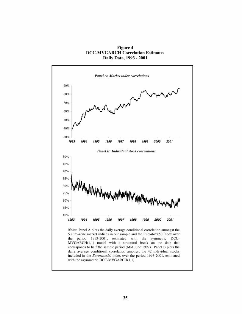
explained by a symmetric process with a structural break in its mean.13 Panel A

of Figure 4 plots the market index average conditional correlation estimated with

the symmetric Model 5, allowing for a structural break in June 1997.

Turning to the correlation patterns amongst the 42 individual stocks in our

sample, the estimation results for selected specifications of the DCC-

MVGARCH model are reported in Table 6. As shown in Panel B of this Table,

we can reject the restriction that both the asymmetric component coefficient θ

and the deterministic time trend coefficient δTrend are equal to zero (Model 1

against Model 3), the null that the former is equal to zero (Model 1 against

13 We also estimated each model without the Eurostoxx50 index, and over the longer sample period 1992-2001, excluding the MIB30 index (because its series starts a year later). We obtained very similar results in all cases, and these are not reported here for brevity.

20

Model 2) and the null that the latter is equal to zero (Model 1 against Model 4)14.

Although the estimated time-trend coefficient is statistically significant, it is very

small (it roughly implies a 1% change in stock correlations over a 10-year

period). We therefore conclude that the salient feature of the process followed by

the conditional correlations amongst the individual stocks included in the

Eurostoxx50 is their asymmetric response to joint bad and good news. In

particular, the estimated asymmetric component coefficient θ in Model 1 is equal

to 0.051, implying a positive response to joint negative return innovations. In

other words, correlations tend to rise after joint negative news more than after

joint positive news. The time series of the estimated asymmetric average

conditional stock return correlation is plotted in Panel B of Figure 4.

A noteworthy feature of all our estimated models, both at the market index level

and at the firm-level, is the strong persistence of the conditional correlation

processes, measured by the parameter β in (26). It ranges from 0.98 to 0.99 in

the index models in Table 5 and it is equal to 0.90 in the model of the individual

stocks in Table 6. In many cases, the sum of the persistence parameter and of

the news parameter (the parameter α in (26)) is close to unity. But the

similarities end there. Average index-level correlation rises, whereas average

stock correlation, in the asymmetric case, actually declines towards the end of

the sample period. The conditional correlation at the market index level appears

to follow a symmetric process, and to be strongly characterised by a structural

break that raises the correlations more than twofold, in a manner that is

consistent with increased economic and financial integration within the euro-

zone. This confirms the results reported by Cappiello, Engle and Sheppard

(2003), and it is consistent with the rise in volatility spillovers noticed by Baele

(2002). In contrast to this, the conditional correlation process at the firm level is

strongly asymmetric, but there appears to be no structural break. As seen in

14 The standard error and associated t-ratio and p-value for Model 1 in Table 6 are not reported because, since we started the maximisation procedure with initial guesses very close to the final estimates, it was impossible to “map out” its curvature, as its gradient was already quite close to zero. Since this is a very lengthy procedure, we did not re-estimate. We therefore rely only on the LR test (Model 1 against Model 4 at the bottom of Table 6) in order to evaluate the significance of the deterministic time trend coefficient.

21

Figure 3, the estimated average correlation between the 42 individual stocks in

our sample rises in connection with the 1997 stock market turmoil and with the

sharp stock market decline world-wide which began in 2002. This provides the

visual justification for the asymmetric component in the conditional correlation

process. Because of the inclusion of this component, the aggregate conditional

correlation series (in the bottom panel of Figure 4), is much smoother than its

unconditional counterpart (Figure 3). Also, because of the strength and the

statistical significance of the asymmetric component in the firm-level correlation

process, it is natural to argue that the spikes in the unconditional correlation plot

are related more to the generalised falls in stock market prices rather than to the

process of integration in the euro-zone.

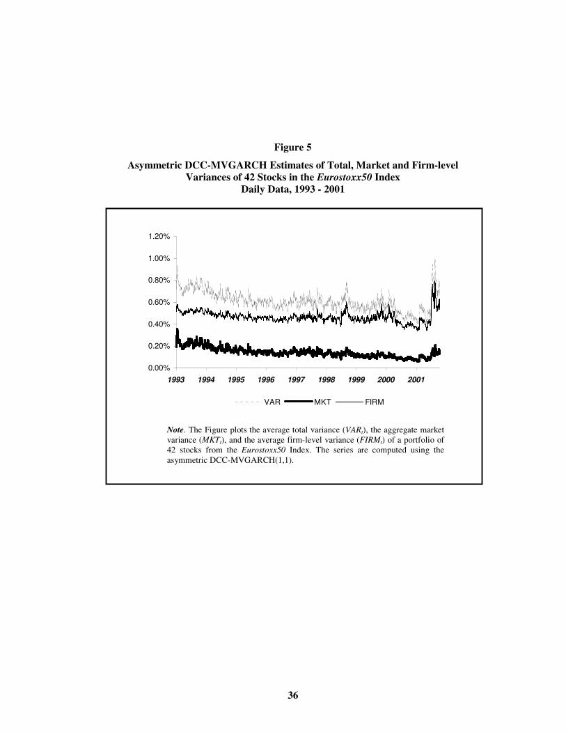
Finally, we use the univariate GARCH volatility estimates given by the first step

of the DCC-MVGARCH estimation procedure in equation (24) to compute a

GARCH version of the average total variance (VARt) of our portfolio of 42

stocks. We then average across the conditional correlation estimates computed

in the second stage of the DCC-MVGARCH estimation procedure to obtain the

conditional version of the aggregate correlation of stocks returns (rt). We can

use this to divide (according to (9)), the aggregate GARCH total variance

measure into conditional market risk (the conditional version of MKTt) and

conditional idiosyncratic risk (the conditional version of FIRMt). The end result

is the plot of the conditional variance of the market portfolio, average firm-level

variance and average total variance reported in Figure 5 for the case when both

volatilities and correlations follow an asymmetric process.

5. Summary and Conclusions Our purpose in this paper has been to examine the trends in market and firm-

level volatility in European equity markets. Using over 2,300 daily observations

from February 1993 to November 2001 on 6 European market indices and 42

stocks from the Eurostoxx50 index, we analysed the time series behaviour of

market risk, idiosyncratic risk, and aggregate correlations between the indices

and between the individual stocks. In addition to extending the CLMX (2001)

22

methodology to provide a full description of the relation between changes in

market risk, aggregate idiosyncratic risk and return correlations, we also applied

the asymmetric version of the DCC-MVGARCH model of Engle (2001) and

Engle and Sheppard (2002) to capture the time series behaviour of the

conditional correlations between the market indexes and between the individual

stocks in the Eurostoxx50 index.

We find that both market risk and aggregate idiosyncratic risk are trended

upwards in our sample, and that the deterministic time trend at work in the latter

is stronger than in the former. The rise in idiosyncratic risk implies that it takes

more stocks to achieve a given level of diversification, and is consistent with the

results reported by CLMX (2001) for United States markets. We also find that

aggregate firm-level return correlations are trended weakly downwards in the

euro-zone. Part of this finding might be explained by the fact that our sample

includes large stocks that have a significant degree of diversification built into

the cash flows associated with their businesses. In contrast to this, however, the

average correlation amongst the 5 euro-zone stock market indices and the

Eurostoxx50 index has risen significantly over our sample period. This, we

argue, is not surprising in view of the ongoing process of economic and financial

integration in the euro-zone area.

In applying the DCC-MVGARCH model to further examine the behaviour of

euro-zone correlations, we find that, consistent with CLMX (2001) and Capiello,

Engle and Sheppard (2003), all our conditional correlation time series estimates

display significant degrees of persistence. At the market index level, we can

reject the restriction that the parameters of the correlation process sum to unity,

but there is strong evidence of a structural break in the mean shortly before the

introduction of the Euro. This explains both the strong persistence of the

correlation time series and its significant rise over the sample period. We also

find that the conditional correlation process is strongly asymmetrical with a

negative but very small deterministic time trend. The asymmetry of the stock

returns correlation process also explains why the skewness of market index

returns, as reported in Table 2, is always negative whereas stock returns have

23

either negative or positive skewness. Our finding that correlations amongst euro-

zone stock returns display a much weaker tendency to decrease than reported by

CLMX (2001) suggests the existence of different correlation dynamics in the

euro-zone area and in the United States, at least over the portion of our sample

period that overlaps (from 1993 to 1997). A number of explanations of this

disparity can be tentatively advanced. Commensurate with a corporate culture in

Europe that emphasis external capital markets somewhat less than in the United

States, companies in Europe have probably pursued less diversification strategies

than in the United States. Another possible explanation is that the tendency for

companies to access the equity market at earlier stages in their life cycle is less

pronounced in Europe than in the United States15. Moreover, the level of average

correlation in our sample, especially in the case of the DCC-MVGARCH

estimates, is generally higher than in the CLMX’s (2001) sample16, implying,

according to (8), a higher ratio of market to total variance and a lower ratio of

firm-level to total variance. This suggests that the portion of total risk

represented by idiosyncratic risk in euro-zone equity markets might be smaller

than in the United States, implying a lower benefit to diversification in the euro-

zone area. In other words, the opportunity-cost of not diversifying is relatively

lower. Part of this difference might be explained by the fact that our sample

comprises large stocks that have a significant degree of built-in diversification.

Nevertheless, our results suggest that fund managers should think through the

full ramifications of seeking more cost-effective diversification by adopting the

passive strategy of investing in market indexes rather than a selection of stocks

from each country.

15 There is the possibility that this tendency might not have been detected by our estimates because we worked with a sample of stocks issued by well established firms (as it must be the case since they are included in the Eurostoxx50 Index). 16 Our sample period and CLMX’s (2001) overlap across the central portion of the 1990s (from 1993 to 1997). CLMX (2001) report that correlations based on 5 years of monthly data decline from 0.28 in the early 1960s to 0.08 in 1997 and that correlations based on 1 year of daily data (more comparable to our correlation measures) decreased from 0.12 in the early 1960s to between 0.02 and 0.04 in the 1990s.

24

Bibliography

Ang, A., Bekaert, G., 1999. International Asset Allocation with Time-Varying Correlations, NBER Working Paper No. 7056. Baks, K.P., Metrick, A., Wachter, J., 2001. Should Investors Avoid All Actively Managed Mutual Funds? A Study in Bayesian Performance Evaluation. Journal of Finance 56, 45-85. Baele, L., 2002. Volatility Spillover Effects in European Equity Markets: Evidence from a Regime-Switching Model, Working Paper. Blake, D., Timmerman, A., 1998. Mutual Fund Performance: Evidence from the UK. European Finance Review 2, 57-77. Bollerslev, T., 1990. Modelling the Coherence in Short-Run Nominal Exchange Rates: a Multivariate Generalised ARCH Approach. Review of Economics and Statistics 72, 498-505. Campbell, J.Y, Lettau, M., Malkiel, B.G., XU, Y., 2001. Have Individual Stocks Become More Volatile? An Empirical Exploration Of Idiosyncratic Risk. Journal of Finance 56, 1-43. Cappiello, L., Engle, R.F., Sheppard, K., 2003. Asymmetric Dynamics in the Correlations of Global Equity and Bond Returns. Working Paper, University of California, San Diego. Coval, J.D., Moskowitz, T.J., 2001. The Geography of Investment: Informed Trading and Asset Prices. Journal of Political Economy.109, 811-841. De Santis, G., Gerard, B., 1997. International Asset Pricing and Portfolio Diversification with Time-Varying Risk. Journal of Finance 52, 1881-1912. Dickey, D.A., Fuller, W.A., 1979. Distribution of the Estimators for Auto-regressive Time Series with a Unit Root. Journal of the American Statistical Association 74, 427-31. Durbin, J., 1970. Testing for Serial Correlation in Least Squares Regression when Some of the Regressors are Lagged Dependent Variables. Econometrica 38, 410-421. Engle, R.F., 2001. Dynamic Conditional Correlation – A Simple Class of Multivariate GARCH Models. Working Paper, University of California, San Diego. Engle, R.F., Sheppard, K., 2001. Theoretical and Empirical Properties of Dynamic Conditional Correlation Multivariate GARCH. Working Paper, University of California, San Diego.

25

Erb, C.B., Harvey, C.R., Viskanta, T.E., 1994. Forecasting International Equity Correlations. Financial Analyst Journal 50, 32-45. Fratzschler, M., 2002. Financial Market Integration in Europe: On the Effects of EMU on Stock Markets. International Journal of Finance and Economics 7, 165-193. Hamilton, J.D., 1994. Time Series Analysis. Princeton University Press, Princeton. Hardouvelis, G., Malliaropulos, D., Priestley, R., 2000. EMU and European Stock Market Integration. CEPR Discussion Paper. Hentschel, L., 1995. All in the Family: Nesting Symmetric and Asymmetric GARCH Models. Journal of Financial Economics 39, 71-104. Longin, F., Solnik, B., 1995. Is Correlation in International Equity Returns Constant: 1960 – 1990?. Journal of International Money and Finance 14, 3-26. Longin, F., Solnik, B., 2001. Extreme Correlation of International Equity Markets, Journal of Finance, 56, 649-676 Newy, W.K., West, D.K., 1987. A Simple, Positive Semi-Definite, Heteroskedasticity and Autocorrelation Consistent Covariance Matrix. Econometrica 55, 703-8. Pesaran, M. H., Pesaran, B., 1997. Working with Microfit 4.0. Oxford University Press, Oxford. Wermers, R., 2000. Mutual Fund Performance: An Empirical Decomposition into Stock-Picking Talent, Style, Transaction Costs, and Expenses. Journal of Finance 55, 1655-1695.

26

Table 1 Stocks Included in the Eurostoxx50 Index

Company Bloomberg Ticker Market Sector Weights (%) 1 ABN AMRO AABA NA BAK 1.59 2 AEGON AGN NA INN 1.55 3 AHOLD AHLN NA NCG 1.87 4 AIR LIQUIDE AI FP CHE 0.89 5 ALCATEL CGE FP THE 1.02 6 ALLIANZ ALThe V GY INN 2.49 7 ASSICURAZIONI GENERALI G IM INN 2.15 8 AVENTIS AVE FP HCA 3.48 9 AXA UAP N.A. INN 2.00 10 BASF BAS GY CHE 1.26 11 BAYER BAY GY CHE 1.40 12 BAYERISCHE HYPO & VEREINSBANK HVM GY BAK 0.75 13 BCO BILBAO VIZCAYA ARGENTARIA BBVA SM BAK 2.39 14 BCO SANTANDER CENTRAL HISP SAN SM BAK 2.46 15 BNP* BNP FP BAK 2.37 16 CARREFOUR SUPERMARCHE CA FP RET 1.97 17 DAIMLERCHRYSLER* DCX GY ATO 1.86 18 DEUTSCHE BANK R DBK GY BAK 2.13 19 DEUTSCHE TELEKOM* DTE GY TEL 2.64 20 E.ON EOA GY UTS 2.39 21 ENDESA ELE SM UTS 1.14 22 ENEL* ENEL IM UTS 0.83 23 ENI* ENI IM ENG 2.22 24 FORTIS B FORB BB FSV 0.98 25 FRANCE TELECOM* FTE FP TEL 1.06 26 GROUPE DANONE N.A. FOB 1.47 27 ING GROEP INGA NA FSV 2.95 28 L'OREAL OR FP NCG 1.52 29 LVMH MOET HENNESSY N.A. CGS 0.55 30 MUENCHENER RUECKVER R* MUV2 GY INN 1.70 31 NOKIA NOK1V FH THE 5.63 32 PHILIPS ELECTRONICS PHIA NA CGS 1.75 33 PINAULT PRINTEMPS REDOUTE PP FP RET 0.49 34 REPSOL YPF REP SM ENG 1.02 35 ROYAL DUTCH PETROLEUM RDA NA ENG 7.63 36 RWE RWE GY UTS 0.98 37 SAINT GOBAIN SAN FP CNS 0.81 38 SAN PAOLO IMI SPI IM BAK 0.70 39 SANOFI SYNTHELABO N.A. HCA 1.81 40 SIEMENS SIE GY THE 2.34 41 SOC GENERALE A SGO FP BAK 1.46 42 SUEZ SZE FP UTS 2.39 43 TELECOM ITALIA TI IM TEL 1.19 44 TELEFONICA TEF SM TEL 3.24 45 TIM* TIM IM TEL 1.22 46 TOTAL FINA ELF FP FP ENG 7.31 47 UNICREDITO ITALIANO UC IM BAK 0.84 48 UNILEVER NV UNA NA FOB 2.49 49 VIVENDI UNIVERSAL N.A. MDI 3.07 50 VOLKSWAGEN VOW GY ATO 0.54

Note. This table reports the stocks included in the Eurostoxx50 as of 23 November 2001 and the weights as of the date of the last reshuffle (19 September 2001) before the end of our sample period (23 November 2001). Asterisks indicate that the series has been dropped from the sample. Descriptors for the market sectors are as follows (Stoxx’s Industry Codes): BAK (Banks), ATO (Auto), INN (Insurance), TEL (Telecom), NCG ((Non-Cyclical Goods and Services), UTS (Utilities), CHE (Chemical), ENG (Energy), THE (Technology), FSV (Financials), HCA (Health Care), FOB (Food & Beverages), RET (Retailer), CGS (Cyclical Goods and Services), CNS (Construction), MDI (Media).

27

Table 2 Summary Statistics for Stock and Market Index Returns

Std. Mean Dev. Skew Sig. Kurt. JB

Panel A: Individula Stocks ABN AMRO 19.10 27.57 -0.17 0.001 4.47 2104 AEGON 32.39 28.33 0.20 0.001 4.19 1848 AHOLD 22.72 25.84 0.26 0.000 2.83 865 AIR LIQUIDE 13.28 27.75 0.24 0.000 2.14 485 ALCATEL 7.68 44.33 -0.97 0.000 17.27 30517 ALLIANZ 16.46 30.45 0.13 0.009 6.76 4398 AVENTIS 21.74 32.79 0.47 0.000 4.56 1957 N.A. 19.58 31.34 -0.12 0.013 3.04 938 BCO BILBAO VIZ. ARGENTARIA 26.41 30.21 0.10 0.040 6.88 4696 BASF 17.87 27.39 0.36 0.000 4.37 1885 BAYER 15.36 26.79 -0.28 0.000 7.21 5031 BAYER. HYPO & VEREINSBANK 12.25 33.02 0.35 0.000 5.31 2755 BNP 10.83 35.28 0.33 0.000 3.21 889 BCO SANTANDER CENTRAL HISP 20.74 32.21 -0.46 0.000 7.29 5346 CARREFOUR SUPERMARCHE 20.93 29.28 0.02 0.623 2.98 896 DAIMLERCHRYSLER -7.40 34.46 -0.01 0.868 1.74 96 N.A. 6.93 26.12 0.06 0.205 3.38 1153 DEUTSCHE BANK R 12.36 30.98 0.20 0.000 6.62 4228 DEUTSCHE TELEKOM 12.67 46.80 0.30 0.000 1.43 125 E.ON 15.66 26.46 0.22 0.000 3.28 1051 ENDESA 19.88 25.79 0.07 0.141 2.36 553 ENEL -6.00 28.02 -0.10 0.335 2.15 101 ENI 19.59 28.55 0.13 0.039 1.33 113 FORTIS B 22.06 26.22 0.10 0.038 3.64 1343 FRANCE TELECOM 19.12 52.42 0.63 0.000 3.33 537 ASSICURAZIONI GENERALI 14.11 26.36 0.17 0.001 2.11 462 ING GROEP 27.16 28.55 -0.48 0.000 8.22 7153 L'OREAL 26.45 32.67 0.10 0.054 1.85 350 N.A. 11.31 33.50 0.40 0.000 4.11 1771 MUENCHENER RUECKVER R 29.12 40.74 -1.72 0.000 31.38 59805 NOKIA 92.62 49.62 -0.08 0.105 5.12 2624 PHILIPS ELECTRONICS 36.53 42.34 -0.18 0.000 3.92 1615 PINAULT PRINTEMPS REDOUTE 25.22 31.22 0.04 0.456 3.03 923 REPSOL YPF 16.54 24.85 0.63 0.000 6.29 4088 ROYAL DUTCH PETROLEUM 16.09 23.35 0.09 0.075 2.79 815 RWE 12.60 27.43 0.48 0.000 5.17 2659 SAINT GOBAIN 30.13 32.67 0.18 0.000 1.95 397 SAN PAOLO IMI 12.53 33.73 0.34 0.000 2.21 524 SIEMENS 16.96 32.02 0.27 0.000 6.54 4407 N.A. 16.00 32.75 0.07 0.152 3.12 983 SOC GENERALE A 13.94 30.62 0.08 0.127 2.30 539 SUEZ 12.31 26.83 0.37 0.000 2.86 855 TELECOM ITALIA 30.41 35.53 -0.26 0.000 5.23 2791 TELEFONICA 26.81 31.70 0.08 0.091 1.77 314 TIM 33.65 37.28 0.23 0.000 0.76 51 TOTAL FINA ELF 17.61 30.21 -0.03 0.527 1.59 256 UNICREDITO ITALIANO 17.85 37.28 0.76 0.000 4.33 2121 UNILEVER NV 15.45 23.98 0.31 0.000 6.45 4382 N.A. 10.23 30.21 0.18 0.000 2.74 770 VOLKSWAGEN 15.34 31.90 0.07 0.161 3.86 1532 Panel B: Market Indices DAX 12.33 34.10 -0.44 0.000 3.72 1,564 CAC40 10.37 19.75 -0.15 0.001 1.88 389 MIB30 13.66 23.56 -0.07 0.188 2.08 417 AEX 13.84 18.10 -0.39 0.000 4.38 2,121 IBEX 12.23 20.43 -0.28 0.000 2.82 881 EUROSTOXX50 13.23 18.03 -0.29 0.000 3.65 1,462

Notes. The table reports summary statistics for stocks included in the Eurostoxx50 on 23 November 2001. The sample period is 1993-2001. Mean and standard deviations are on a 1-year basis. JB denotes the Jarque-Bera statistics. The Kurtosis and the JB statistics are different from zero at the 0.1 percent level for all stocks in the sample.

28

Figure 1

Aggregate Market, Firm-Level and Total Variance

of 42 Stocks in the Eurostoxx50 Index

Panel A: Equal Weights

Note. This figure plots both the equally-weighted (Panel A) and the value-weighted (Panel B) aggregate market variance (MKTt), average firm-level variance (FIRMt) and average total variance (VARt) monthly time series, computed using daily closing prices of 42 stocks included in the Eurostoxx50 index over the sample period 1993-2001.

0.0%

0.5%

1.0%

1.5%

2.0%

2.5%

3.0%

3.5%

4.0%

4.5%

1993 1994 1995 1996 1997 1998 1999 2000 2001

0.0%

0.5%

1.0%

1.5%

2.0%

2.5%

3.0%

3.5%

4.0%

4.5%

1993 1994 1995 1996 1997 1998 1999 2000 2001

MKT FIRM VAR

Panel B: Value weights

29

Figure 2

The Ratio of Firm-Level to Total Variance and Average Return Correlations amongst 42 Eurostoxx50 Stocks

Note. Panel A plots the ratio of the average firm-level variance (FIRMt) to the average total variance (VARt) monthly time series. Panel B depicts the average correlation time series. Both series are computed using the sample of 42 stocks over the sample period 1993-2001.

Panel A: Ratio of firm-level to total variance

30%

40%

50%

60%

70%

80%

90%

100%

1993 1994 1995 1996 1997 1998 1999 2000 2001

0%

10%

20%

30%

40%

50%

60%

70%

80%

1993 1994 1995 1996 1997 1998 1999 2000 2001

Panel B: Average correlations

30

Figure 3

Average Correlation amongst 5 Euro-zone Market Indexes and the Eurostoxx50 Index

Notes. This Figure plots the time series of monthly average correlation amongst 5 Euro-zone national stock market indices (ie., the DAX, CAC40, MIB30, AEX, IBEX) and the Eurostoxx50 index.

40%

50%

60%

70%

80%

90%

100%

1993 1994 1995 1996 1997 1998 1999 2000 2001

31

Table 3 Unit Root Tests on Aggregate Returns, Variances and Correlations

CV DF ADF1 ADF2 F-Test

Individual Stocks

FIRMt Intercept, no trend Intercept and linear trend

-2.89 -3.45

-3.95 -5.23

-4.21 -6.23

-3.01 -4.84

MKTt Intercept, no trend Intercept and linear trend

-2.89 -3.45

-5.67 -6.24

-4.65 -5.26

-3.78 -4.45

rt

Intercept, no trend Intercept and linear trend

-2.89 -3.45

-5.68 -5.65

-4.07 -4.04

-3.30 -3.28

Market Indexes

rt

Intercept, no trend Intercept and linear trend

-2.89 -3.45

-4.95 -7.62

-4.10 -7.46

-2.67 -5.57

620.01 (.000)

Notes. This Tables reports Dickey-Fuller (DF) tests and augmented Dickey-Fuller (ADF1 and ADF2, the numbers denoting the order of augmentation) tests. CV denotes the critical value at the 5 percent level. All variables are defined in the text. F-test denotes critical value and significance level (in brackets) of the test statistic under the null that the trend coefficient is zero and the series contains a unit root.

32

Table 4 Specification and Wald-Type Tests

Static Model

Dynamic Model

DW-stat.

� (%) (t-stat.)

� (%) (t-stat.)

� (t-stat.)

h-stat. (sign.)

Wald-stat. (sign.)

Individual Stocks

FIRMt

.86 .00 (0.01)

.0031 (3.22)

.57 (6.94)

8.52 (.003)

10.38 (0.01)

MKTt

1.11 -.00 (0.46)

.0023 (2.33)

.44 (5.00)

.009 (0.92)

5.44 (0.02)

rt

.96 16.66

(4.07) -.0076 (0.22)

.51 (5.95)

2.60 (0.10)

.05 (0.82)

Market Indexes

rt

1.41 38.40

(7.09) .1937 (5.24)

.29 (3.04)

5.08 (0.02)

27.40 (0.00)

Notes. This tables reports estimates of the parameters of the model of the average firm-level variance (FIRMt), market variance (MKTt) and average correlation (rt) series with a deterministic time trend. All variables are defined in the text. DW denotes the Durbin-Watson statistics of the static model from (22). All other columns report estimated coefficient and t-statistics for the dynamic model as in (23). The rightmost columns report the Durbin’s h-statistic of the null that the dynamic model residuals are not first-order autocorrelated and the Wald statistic (in both cases with the associated significance levels) of the restriction that � is equal to zero. All the Wald-Test statistics, standard errors and significance levels have been computed using a Newy-West adjusted variance–covariance matrix with Parzen weights to correct for heteroschedasticity and autocorrelation.

Static Model:

yt = � +�t + ut ut ~ i.i.d. N(0, � 2)

Dynamic Model: yt = � + � yt-1 + �t + ut ut ~ i.i.d. N(0, � 2)

33

Table 5

DCC-MVGARCH Estimates of Market Indexes Daily Data, 1993 - 2001

Panel A

Model Restriction Coefficient Coefficient estimate T-Ratio p-value 1 Q1 = Q2 Q1/2 .799 θ = 0 α .010 7.74 .000 β .986 410.70 .000 δTrend -.000 1.86 .061 2 Q1 = Q2 Q1/2 .799 θ = 0 α .014 10.74 .000 δTrend = 0 β .978 374.51 .000 3 Q1 = Q2 Q1/2 .799 θ = 0 α .007 12.72 .000 δTrend = 0 β .993 1807.09 .000 α + β = 1 4 θ = 0 Q1 .312 δTrend = 0 Q2 .798 α .009 17.52 .000 β .989 1686.47 .000 5 δTrend = 0 Q1 .312 Q2 .798 α .012 11.66 .000 β .987 986.93 .000 θ -.002 -3.83 .000

Panel B Unrestricted Model

ln(|ΣΣΣΣUR|) Restricted Model

ln(|ΣΣΣΣR|) LR Statistic Significance Level

Restriction Rejection

2 -5.0580 3 -5.0798 50.47 .000 Yes 4 -4.8310 2 -5.0580 525.50 .000 Yes 5 -4.8309 4 -4.8310 .23 .597 No

LR = T ln(|ΣUR|)-ln(|ΣR|) ∼ χ2(q) T = number of observations (2,315)

ΣUR = covariance matrix of the residuals of the unrestricted model ΣR = covariance matrix of the residuals of the restricted model χ2(q) = Chi-Squared distributions with q degrees of freedom

q = number of restrictions (q = 15 for Model 4 vs. 2, q = 1 in all other tests)

Notes. Panel A of this Table reports coefficients, t-statistics and p-values for various specifications of the DCC-MVGARCH model of conditional correlations amongst 6 euro-zone market indexes, including the Eurostoxx50 index, over the period 1993-2001. Panel B reports Likelihood Ratio (LR) test statistics and their significance level.

34

Table 6

DCC-MVGARCH Estimates of 42 Eurostoxx50 Stocks Daily Data, 1993 - 2001

Panel A

Model Restriction Coefficient Coefficient estimate T-Ratio p-value

1 Q1 = Q2 α .056 58.00 .000 β .899 12011.98 .000 θ .051 56.42 .000 δTrend .000 - 2 Q1 = Q2 α .005 419.89 .000 θ = 0 β .904 10793.04 .000 δTrend -.000 -18.68 .000 3 Q1 = Q2 α .005 16.57 .003 θ = 0 β .903 2784.11 .000 δTrend = 0 4 Q1 = Q2 α .003 15.68 .000 δTrend = 0 β .978 627.35 .000 θ .000 .39 .701

Panel B

Unrestricted Model

ln(|ΣΣΣΣUR|) Restricted Model

ln(|ΣΣΣΣR|) LR Statistic Significance Level

Restriction Rejection

1 -5.7840 2 -6.7771 2273.26 .000 Yes 1 -5.7840 3 -6.7782 2275.71 .000 Yes 1 -5.7840 4 -12.8915 16268.98 .000 Yes

LR = T ln(|ΣUR|)-ln(|ΣR|) ∼ χ2(q) T = number of observations (2,289)

ΣUR = covariance matrix of the residuals of the unrestricted model ΣR = covariance matrix of the residuals of the restricted model χ2(q) = Chi-Squared distributions with q degrees of freedom

q = number of restrictions (q = 2 for Model 1 vs. 3, q = 1 in all other tests)

Notes. Panel A of this Table reports the coefficients, t-statistics and p-values for the DCC-MVGARCH model of conditional correlations amongst 42 stocks (k = 42) included in the Eurostoxx50 index over the sample period 1993- 2001. Variables and their coefficients are defined in the text. Panel B reports Likelihood Ratio (LR) test statistics and their significance level.

35

Figure 4 DCC-MVGARCH Correlation Estimates

Daily Data, 1993 - 2001

Notes. Panel A plots the daily average conditional correlation amongst the 5 euro-zone market indices in our sample and the Eurostoxx50 Index over the period 1993-2001, estimated with the symmetric DCC-MVGARCH(1,1) model with a structural break on the date that corresponds to half the sample period (Mid June 1997). Panel B plots the daily average conditional correlation amongst the 42 individual stocks included in the Eurostoxx50 index over the period 1993-2001, estimated with the asymmetric DCC-MVGARCH(1,1).

Panel A: Market index correlations

30%

40%

50%

60%

70%

80%

90%

1993 1994 1995 1996 1997 1998 1999 2000 2001

10%

15%

20%

25%

30%

35%

40%

45%

50%

1993 1994 1995 1996 1997 1998 1999 2000 2001

Panel B: Individual stock correlations

36

Figure 5

Asymmetric DCC-MVGARCH Estimates of Total, Market and Firm-level Variances of 42 Stocks in the Eurostoxx50 Index

Daily Data, 1993 - 2001

Note. The Figure plots the average total variance (VARt), the aggregate market variance (MKTt), and the average firm-level variance (FIRMt) of a portfolio of 42 stocks from the Eurostoxx50 Index. The series are computed using the asymmetric DCC-MVGARCH(1,1).

0.00%

0.20%

0.40%

0.60%

0.80%

1.00%

1.20%

1993 1994 1995 1996 1997 1998 1999 2000 2001

VAR MKT FIRM

Institute for International Integration StudiesThe Sutherland Centre, Trinity College Dublin, Dublin 2, Ireland