Statistics & Operations Research Transactions SORT 37 (1) January-June 2013, 57-78 Statistics & Operations Research Transactions c Institut d’Estad´ ıstica de Catalunya [email protected] ISSN: 1696-2281 eISSN: 2013-8830 www.idescat.cat/sort/ New insights into evaluation of regression models through a decomposition of the prediction errors: application to near-infrared spectral data Mar´ ıa Isabel S´ anchez-Rodr´ ıguez 1,* , Elena S´ anchez-L´ opez 2 , Jos´ eM a Caridad 1 , Alberto Marinas 2 , Jose M a Marinas 2 and Francisco Jos´ e Urbano 2 Abstract This paper analyzes the performance of linear regression models taking into account usual criteria such as the number of principal components or latent factors, the goodness of fit or the predictive capability. Other comparison criteria, more common in an economic context, are also considered: the degree of multicollinearity and a decomposition of the mean squared error of the prediction which determines the nature, systematic or random, of the prediction errors. The applications use real data of extra-virgin oil obtained by near-infrared spectroscopy. The high dimensionality of the data is reduced by applying principal component analysis and partial least squares analysis. A possible improvement of these methods by using cluster analysis or the information of the relative maxima of the spectrum is investigated. Finally, obtained results are generalized via cross- validation and bootstrapping. MSC: 62H25, 62J05, 62Q99. Keywords: Principal components, partial least squares, multivariate calibration, near-infrared spectroscopy. 1. Introduction Principal component analysis (PCA) and partial least squares (PLS) are widely used in linear modelling when the number of explanatory variables greatly exceeds the number of observations. PCA and PLS calculate, from the explanatory variables, a reduced * Corresponding author e-mail: [email protected] 1 Dep. Estad´ ıstica, Econometr´ ıa, I.O., Org. Empresas y Ec. Aplicada. Avda. Puerta Nueva, s/n. 14071. University of C´ ordoba. C´ ordoba. Spain. 2 Dep. Qu´ ımica Org´ anica. Campus de Excelencia Agroalimentario ceiA3. Edificio C-3 (Marie Curie-Anexo). Campus de Rabanales. 14014. University of C´ ordoba. C´ ordoba. Spain. Received: April 2012 Accepted: October 2012

Welcome message from author
This document is posted to help you gain knowledge. Please leave a comment to let me know what you think about it! Share it to your friends and learn new things together.
Transcript

Statistics & Operations Research Transactions
SORT 37 (1) January-June 2013, 57-78
Statistics &Operations Research
Transactionsc© Institut d’Estadıstica de Catalunya
[email protected]: 1696-2281eISSN: 2013-8830www.idescat.cat/sort/
New insights into evaluation of regression models
through a decomposition of the prediction errors:
application to near-infrared spectral data
Marıa Isabel Sanchez-Rodrıguez1,∗, Elena Sanchez-Lopez2, Jose Ma Caridad1,
Alberto Marinas2, Jose Ma Marinas2 and Francisco Jose Urbano2
Abstract
This paper analyzes the performance of linear regression models taking into account usual criteria
such as the number of principal components or latent factors, the goodness of fit or the predictive
capability. Other comparison criteria, more common in an economic context, are also considered:
the degree of multicollinearity and a decomposition of the mean squared error of the prediction
which determines the nature, systematic or random, of the prediction errors. The applications use
real data of extra-virgin oil obtained by near-infrared spectroscopy. The high dimensionality of
the data is reduced by applying principal component analysis and partial least squares analysis.
A possible improvement of these methods by using cluster analysis or the information of the
relative maxima of the spectrum is investigated. Finally, obtained results are generalized via cross-
validation and bootstrapping.
MSC: 62H25, 62J05, 62Q99.
Keywords: Principal components, partial least squares, multivariate calibration, near-infrared
spectroscopy.
1. Introduction
Principal component analysis (PCA) and partial least squares (PLS) are widely used in
linear modelling when the number of explanatory variables greatly exceeds the number
of observations. PCA and PLS calculate, from the explanatory variables, a reduced
∗ Corresponding author e-mail: [email protected] Dep. Estadıstica, Econometrıa, I.O., Org. Empresas y Ec. Aplicada. Avda. Puerta Nueva, s/n. 14071. University
of Cordoba. Cordoba. Spain.2 Dep. Quımica Organica. Campus de Excelencia Agroalimentario ceiA3. Edificio C-3 (Marie Curie-Anexo).
Campus de Rabanales. 14014. University of Cordoba. Cordoba. Spain.
Received: April 2012
Accepted: October 2012

58 New insights into evaluation of regression models through a decomposition...
number of components or latent factors orthogonal among themselves. These compo-
nents or factors are obtained as linear combinations of the explanatory variables, for
PCA explaining the variability among these variables and, for PLS maximizing the co-
variance between each explanatory variable and the response one. Both methodologies
reduce the dimensionality of the space of explanatory variables as the information pro-
vided by these variables is summarized in only a few ones.
PCA and PLS have been used in the last decades in some chemometric areas
such as, for example, in pattern recognition (in this context, PCA or PLS linear
discriminant analyses establish classification models based on experimental data in
order to assign unknown samples to a sample class) and in multivariate calibration,
in which PCA or PLS regression models predict a numeric variable as a function
of several explanatory ones. Although papers comparing the goodness between PCA
and PLS are well-known, most of them even considering PLS preferable to PCA for
both regression and discrimination (see, for example, Frank and Friedman (1993) or
Barker and Rayens (2003)), the fact is that PCA (besides PLS) is still widely used
nowadays in chemometrics. Papers such as Gurdeniz and Ozen (2009), Lopez-Negrete
de la Fuente, Garcıa-Munoz and Blegler (2010), Mevik and Cederkvist (2004), Nelson,
MacGregor and Taylor (2006) and Yamamoto et al. (2009) can be cited as examples
of using PCA in discrimination and calibration. For this reason, this paper revisits
the comparison between PCA and PLS regressions in new terms. Firstly, the possible
improvement of the regression models incorporating causal additional information of
data is analyzed. Secondly, a proposed decomposition of the prediction errors makes it
possible to determine the nature of these errors and evaluate their predictive capacity.
In this paper, the described methodology is applied to data obtained by near-
infrared (NIR) spectroscopy. The NIR methods are used in food chemistry providing
fast, reliable and cost-effective analytical procedures which, contrary to some others
– such as gas chromatography – require no or little sample manipulation. Even though
the data acquisition process is relatively easy for all spectral techniques, interpretation
of spectra can be difficult. Separation techniques, such as gas chromatography, lead
to discrete information including several usually well-defined, separated peaks from
which, on proper integration, the content of various chemical components in the sample
can be determined. On the contrary, spectroscopy generates continuous information,
rich in both isolated and overlapping bands attributed to vibration of chemical bonds in
molecules, which leads to the availability of multivariate data matrices. In this context,
the use of mathematical and statistical procedures allows us to extract the maximum
useful information from data (Berrueta, Alonso-Salces and Heberger, 2007).
There are many chemometric papers establishing comparison criteria of models.
Thus, for example, Gowen et al. (2010) or Li, Morris and Martin (2002) propose some
measures to determine the optimal number of latent factors in PLS regression mod-
els; Anderson (2009) compares diverse models of PLS regression as a function of their
stability; Andersen and Bro (2010) or Reinaldo, Martins and Ferreira (2008) propose
several selection criteria for variables in multiple calibration models; and Mevik and

Sanchez-Rodrıguez, M. I. et al. 59
Cerderkvist (2004) provide estimators of the mean squared error of prediction (MSEP)
in PCA and PLS regression models. The aim of this paper is to compare PCA and PLS
regression models on the basis of some criteria such as the number of latent factors or
components, the goodness of fit and the predictive capability. However, this study goes
a step further, incorporating an approach usually associated with an economic context.
The degree of multicollinearity (absent when the regressors of the model are uncorre-
lated among themselves) is considered. Moreover, a decomposition of MSEP is pro-
posed in order to point out the nature, systematic or random, of the prediction errors. As
a final conclusion, the development of the study highlights the potential of the PLS re-
gression.
There are several examples in the literature on the application of PCA and PLS re-
gression models to near-infrared spectral data from oils and fats. For instance, Dupuy et
al. (1996), Gurdeniz and Ozen (2009), Kasemsumran et al. (2005) and Ozturk, Yalcin
and Ozdemir (2010) use these multivariate calibration models to predict the content of
some olive oil compounds in order to detect possible adulteration with some other veg-
etable oil. In the present study, the application is carried out by using NIR spectral data
of extra-virgin olive oil and estimates the capability of the models to predict the oleic
acid content. However, our approach could be used to estimate some other chemicals or
features of importance in food chemistry from spectral data (see Mevik and Cederkvist
(2004)). Firstly, the regression models are fitted by applying PCA and PLS from all the
variables associated to different wavelengths of the spectrum (considering the matrix
of data as a black box). Later on, models incorporating information provided by the
relative maxima of the curve are estimated, because the principal components and the
factors are obtained, in an independent manner, in each spectral peak. Then, PCA and
PLS regressions are applied in combination with cluster analysis, a multivariate statisti-
cal technique that uses a measure of distance or similarity to classify a set of variables
or cases in clusters of variables or cases, respectively, similar among themselves; in
this case, components and factors are obtained independently in each cluster of wave-
lengths. The above-mentioned criteria are calculated for each model in order to evaluate
their performance. For models in which PCA or PLS are carried out in an independent
manner in different parts of the spectrum and so the resulting components or factors
are not orthogonal among themselves, the degree of multicollinearity is also considered.
Finally, techniques of cross-validation and bootstrapping are incorporated to extend the
previous results to more general applications.
2. Review of selection criteria in regression models
2.1. Common comparison criteria
a) Goodness of fit. Let s2Y and s2
Ybe the respective variances of the observations,
y1,y2, . . . ,yn, of the dependent variable Y , and the corresponding predictions,

60 New insights into evaluation of regression models through a decomposition...
y1, y2, . . . , yn, in a regression model. The coefficient of determination, R2 = s2
Y/s2
Y ,
ranges in the interval [0,1] by definition and, expressed as a %, indicates the
percentage of variability of the dependent variable explained by the regression
model. Obviously, a model is better as the coefficient of determination approaches
1. The adjusted coefficient of determination, R2, is calculated from R2, taking
into account the number of observations and the number of the regressors in the
regression, in such a way that the goodness of fit is not overestimated.
The mean squared error of calibration, MSEC = ∑ni=1 (yi − yi)
2 /n, takes values
nearer to 0 for a good fit, but it is non-dimensionless, that is, it depends on the
units of measure of the variable.
There are other measures of the goodness of fit, that are not contemplated in this
study, based on the likelihood criterion (see Burnham and Anderson (2004)).
b) Predictive capability. Given the predictions for the future t observations, yn+1,
yn+2, . . . , yn+t , of a certain regression model, the mean squared error of the pre-
diction, MSEP=∑tj=1 (yn+ j − yn+ j)
2 /t, evaluates the predictive capability of a re-
gression model. The predictive capability of a model is obviously better as MSEP
approaches 0, taking into account that it also depends on the measurement units.
As is indicated by Berrueta et al. (2007), the ideal situation is when there are
enough data available to create separate test set completely independent from the
model building process (this validation procedure is known as external validation).
When an independent test set is not available (e.g., because cost or time constraints
make it difficult to increase the sample size), MSEP has to be estimated from
the learning data, that is, the data used to train the regression. In this context,
Mevik and Cederkvist (2004) present several estimators for MSEP, based on cross-
validation or bootstrapping: Let X=[X1|X2|...|Xp] be the matrix containing the
explanatory variables in a regression model and let Y be the dependent variable.
For a set of n observations, it is assumed that L = {(xi,yi) : i = 1, . . . ,nL} is a
learning data set (of nL observations) and T = {(xnL+i,ynL+i) : i = 1, . . . ,nT} is a
test data set (of size nT ). Besides, fL is a predictor trained on L. When L is divided
randomly into K segments, L1,L2, . . . ,LK , of roughly equal size (n1,n2, . . . ,nK),
fk is a predictor trained on L\Lk. Finally, R bootstrap samples are drawn in L,
L∗1,L
∗2, . . . ,L
∗R, and f ∗r is a predictor trained on L∗
r . In the described context, Mevik
and Cederkvist (2004) present the MSEP estimators shown in Table 1.
c) Number of regressors. Attending to the parsimony principle, if some regression
models present similar characteristics in terms of goodness of fit, predictive
capacity and multicollinearity, the simplest among them, i.e. the one with the
smallest number of regressors, is considered the best.

Sanchez-Rodrıguez, M. I. et al. 61
Table 1: MSEP estimators adopted from Mevik and Cederkvist (2004).
MSEP Estimator Definition
Test set estimate MSEPtest =1
nT
nT
∑i=1
( fL (xnL+i)− ynL+i)2(= MSEP)
Apparent MSEP MSEPapp =1
nL
nL
∑i=1
( fL (xi)− yi)2(= MSEC)
Cross-validation MSEPcv.K =1
nL
K
∑k=1
∑i∈Lk
( fk (xi)− yi)2
Adjusted
cross-validation
MSEPadj.cv.K = MSEPcv.K +MSEPadj, where
MSEPadj = MSEPapp −1
nL
K
∑k=1
nk
nL∑
i 6∈Lk
( fk (xi)− yi)2
Naive bootstrap
estimate
MSEPnaive =1
R
R
∑r=1
1
nL
nL
∑i=1
( f ∗r (xi)− yi)2
Ordinary bootstrap
estimate
MSEPboot = MSEPapp +Biasapp, where
Biasapp =1
R
R
∑r=1
(1
nL
nL
∑i=1
( f ∗r (xi)− yi)2 −
1
nL
nL
∑i=1
( f ∗r (xri )− yr
i )2
),
where(xr
i ,yri
)is the ith observation of the rth bootstrap sample
Bootstrap smoothed
cross-validation
MSEPBCV =1
nL
nL
∑i=1
1
R−i∑
r:i 6∈L∗r
( f ∗r (xi)− yi)2,
where R−i is the number of bootstrap samples excluding observation i
The 0.632 estimate MSEP0.632 = 0.632 ·MSEPBCV +(1−0.632) ·MSEPapp,
where 0.632 ≈ 1− e−1 is approximately the average fraction
of distinct observations in each bootstrap data set
In PCA, the Kaiser criterion is the default in SPSS and most statistical software
(but many authors do not recommend to use it as the only cut-off criterion as it
tends to extract too many factors): Let X∗1 ,X
∗2 , . . . ,X
∗p be the standardized variables
of the explanatory variables, X1,X2, . . . ,Xp. When a random sample of dimension n
is considered, X∗ = [X∗1 |X
∗2 | · · · |X
∗p ] is a matrix of dimension n× p. Then, X∗TX∗ is
a square p× p matrix and has p eigenvalues, λ1,λ2, . . . ,λp. The eigenvalueλk rep-
resents the variance of the k-th principal component (or factor), k = 1, . . . , p. The
Kaiser criterion suggests that those factors with eigenvalues equal or higher than 1

62 New insights into evaluation of regression models through a decomposition...
should be retained (taking into account that the variables are standardized and so
the average of the eigenvalues is precisely 1).
In PLS analysis, the criterion of the first increase of the mean squared error
of prediction is considered: the number of latent factors taken into account is
h∗ = min{h > 1 : MSEP(h+1)−MSEP(h)> 0}, where MSEP(h) the mean squared
error of prediction of the regression model with h factors.
Gowen et al. (2010) show that the over-fitting in a regression model entails
some additional problems, such as the introduction of noise in the regression
coefficients. More specifically, their paper presents some measures for preventing
the over-fitting in PLS calibration models of NIR spectroscopy data, investigating
the use of both model bias and variance simultaneously in selecting the number
of latent factors to include in the model. Initially, the authors consider the Durbin-
Watson statistic:
DW =∑
pi=1 (bi −bi−1)
2
∑pi=0 b2
i
,
being p the number of the regressors and b0,b1, . . . ,bp the coefficients of the mul-
tiple regression model. The named regression vector measure, RVM, is calculated
by rescaling DW from 0 to 1. Then, a bias measure, BM, is obtained once the root
of the mean squared error of calibration, RMSEC, is rescaled from 0 to 1. Gowen
et al. (2010) propose to obtain the measures RVM j and BM j for models with j latent
factors or components, varying j. Finally, the optimal number of latent factor to
consider in a PLS regression model is j∗ if the minimum of the sum RVM j + BM j
is obtained for j = j∗.
2.2. Other comparison criteria
In this section, other comparison criteria, more frequent in economics research, are pro-
posed. Thus, for example, the decomposition of MSEP provided in d) below is devel-
oped in EViews, a program of econometric analysis. Similarly, Essi, Chukuigwe and
Ojekudo (2011), Greenberg and Parks (1997), Mynbaev (2011), Spanos and McGuirk
(2002) and Yamagata (2006) deal with the multicollinearity under different hypotheses
in an economic context. These new criteria establish additional arguments to the ones
proposed in a)-c) and can assist in selecting the most adequate model.
d) Decomposition of MSEP. In Section 2.1.b, MSEP has been established as a
criterion for evaluating the predictive capability of a model which, in general
terms, is better as MSEP approaches 0. But this issue can be dealt more in depth,
trying to determine the causes of the prediction errors.

Sanchez-Rodrıguez, M. I. et al. 63
Around 1920, Fisher introduced analysis of variance (ANOVA), a collection of
statistical procedures in which the observed variance in a particular variable is
partitioned into components attributable to different sources of variation. Diverse
authors, e.g. Climaco-Pinto et al. (2009), Mark (1986), Mark and Workman
(1986), Zwanenburg et al. (2011) have used the ANOVA in a chemometric context.
We use this technique to decompose MSEP into three components, with the aim
of investigating if there is any systematic cause that produces the prediction errors
or if they are randomly distributed.
Given the predictions for the future t observations, yn+1, yn+2, . . . , yn+t , of a certain
regression model, y and y are the means of the observations and the predictions,
respectively, sY and sY
are the corresponding standard deviations and sYY
is the
covariance. Then, the MSEP,
MSEP =1
t
t
∑j=1
(yn+ j − yn+ j)2 =
1
t
t
∑j=1
y2n+ j +
1
t
t
∑j=1
y2n+ j −
2
t
t
∑j=1
yn+ jyn+ j,
can be decomposed, once the terms(
y− y)2
and 2sYY
are added and subtracted,
in the following way
MSEP =(
y− y)2
+(sY − s
Y
)2+2(sY s
Y− s
YY
)= EB +EV +ER,
or, equivalently, by the identity
1 =EB
MSEP+
EV
MSEP+
ER
MSEP=UB +UV +UR,
where UB is the part of MSEP corresponding to the bias, representing systematic
errors in the prediction; UV indicates the difference between the variability of the
real values and the variability of the observed ones; finally, UR shows the random
variability in the prediction errors.
The decomposition of MSEP evidences that the predictions are affected by sys-
tematic and random errors. Random errors are, in general, low in absolute value,
resulting from the additive effect of many insignificant events (detected with dif-
ficulty) and so inherent to a process. This kind of error can only be reduced with
the increasing of the sample size, and fluctuate around a constant value, being dis-
tributed as a white noise. However, systematic errors are usually associated with
an identifiable cause, such as an interference in the observation process or a defect
of calibration in the instrument of measurement. They usually originate in a great
fluctuation in the evolution of a process and must be detected and eliminated (for

64 New insights into evaluation of regression models through a decomposition...
example, this is the objective of statistical quality control or the aim of papers such
as Guldberg et al. (2005) or Vasquez and Whiting (2006)).
A model is obviously better as MSEP approaches 0 (taking into account that
MSEP is not upperly bounded and depends on the unit of measurement). But,
using the proposed decomposition, if MSEP shows a great percentage attributable
to systematic errors, this aspect indicates that there is some detectable cause
originating these deviations in the predictions. This cause must be detected in order
to eliminate systematic errors. Thus, a great percentage of MSEP attributable to
systematic prediction errors indicates that the fit model can be improved in some
sense. Nevertheless, this improvement is difficult if the predictions generated by a
model have a random nature.
However, the study of the statistical general linear model (in particular, the mul-
tivariate linear regression model) assumes the random nature of its perturbations
(which must be, by hypotheses, centered, homoscedastic, uncorrelated and nor-
mally distributed random variables). And so the presence of systematic errors in
the predictions (represented by a high UB ratio) or the discrepancy between the
variability of the real and the observed values (represented by a high UV ratio)
prevent the validation of the fitted model, since these facts point out the absence
of the hypotheses of randomness and homoscedasticity.
Definitively, the ideal situation for evaluating the predictive capability of a model
is presented when MSEP has a value nearer to 0 and besides UB = 0, that is,
systematic errors do not exist in the prediction; UV = 0, which indicates that the
variability of the real values is the same as that of the predictions; and UR = 1,
which corresponds to random prediction errors.
e) Possible existence of multicollinearity1. In the fit of a regression model, it is
frequent the appearance of a certain linear relationship among the regressors,
which can be even exact (for example, when the number of cases is lower than
the number of explanatory variables). The presence of multicollinearity in the
regression makes that the least squares estimators obtained are not, in general, very
precise. Although these estimators are still linear, unbiased and efficient (Gauss-
Markov theorem), the multicollinearity complicates the precise quantification of
the effect of each regressor on the dependent variable, because the variances of the
estimators are high.
1. In PCA and PLS regressions, the orthogonal character of the components or factors guarantees the absence ofmulticollinearity in the model. In this paper, multicollinearity is evaluated in models whose components or factors areobtained applying PCA or PLS to different parts of the spectrum, in an independent manner. Thus, these components orfactors are uncorrelated only in the corresponding spectral part.

Sanchez-Rodrıguez, M. I. et al. 65
In a multiple linear regression model, the estimator of the variance of a certain
coefficient, β j, is given by the expression
Var
(β j
)=
σ2
p(
1−R2j
)s2
j
, j = 1, . . . , p,
where σ2 is the estimation of the disturbance variance, assumed to be constant by
the hypothesis of homoscedasticity; p is the number of explanatory variables in
the model; R2j is the coefficient of determination of the regression of the variable
X j on the rest of the explanatory variables; and s2j is the observed variance of X j.
The variance inflation factor, VIF, is defined as the ratio between the observed
variance and the variance existing when X j is uncorrelated to the rest of the
regressors of the model (and, then, R2j = 0). Some authors consider that there is
a grave multicollinearity when VIF
(β j
)> 10 for any j = 1, . . . , p, that is, when
R2j > 0.90. Some computational programs (SPSS, for example) define the term
“tolerance” as Tj = 1−R2j ; in this case, a serious multicollinearity is identified
when Tj < 0.10 for any j = 1, . . . , p.
Then, let X∗TX∗ be the matrix defined in Section 2.1.c (X∗ contains the standard-
ized observations). As indicated in that section, it is a square matrix of dimension
p and, therefore, has p eigenvalues. In this case, its condition number, κ, is de-
fined as the root of the ratio between the highest eigenvalue (λmax) and the lowest
one (λmin). The condition number measures the sensitivity of the least-squares es-
timates to small changes in the data. The multicollinearity can be considered as
serious if κ (which is not affected by the measurement units because it is calcu-
lated, as stated above, from standardized variables) ranges between 20 and 30; if
κ is greater than 30, the multicollinearity is very serious.
3. Materials and methods
3.1. Acquisition of spectral data
This work is based on data obtained from olive oil from different olive varieties (mainly
‘Zaity’, ‘Arbequina’, ‘Frantoio’, ‘Picual’ and ‘Hojiblanca’) harvested in the 2005/06,
2006/07, 2007/08 and 2008/09 seasons. Samples correspond to Andalusian olive oils
principally, though some others from Tarragona and Edleb (Syria) have also been
included. There are 302 cases in total. Olive oil was either extracted by the producers
through a two-phase centrifugation system or by the staff of the Agronomy Department
of University of Cordoba via the Abencor System. This system reproduces the industrial

66 New insights into evaluation of regression models through a decomposition...
process on the laboratory scale and follows the same stages of grinding, beating,
centrifugation and decantation.1H-NMR analyses were carried out at the NMR Service of the University of Sevilla
on a Bruker Avance spectrometer (Kahlsruhe, Germany), by using a resonance fre-
quency of 500.2MHz and a direct-detection 5mm QNP 1H/15N/13C/31P probe. De-
termination of oleic acid content was carried out following the method suggested by
Guillen and Ruiz (2003). NIR spectra were obtained by the staff of the Organic Chem-
istry Department of the University of Cordoba within 15 days after reception of the
samples, which where kept in the fridge so that properties were not modified (Baeten
et al., 2003). The instrument employed for spectra collection was available at the Cen-
tral Service of Analyses (SCAI) at the University of Cordoba. It consisted of a Spectrum
One NTS FT-NIR spectrophotometer (Perkin Elmer LLC, Shelton, USA) equipped with
an integrating sphere module. Samples were analyzed by transflectance by using a glass
petri dish and a hexagonal reflector with a total transflectance pathlength of approxi-
mately 0.5 mm. A diffuse reflecting stainless steel surface placed at the bottom of the
cup reflected the radiation back through the sample to the reflectance detector. The spec-
tra were collected by using Spectrum Software 5.0.1 (Perkin Elmer LLC, Shelton, USA).
The reflectance (log 1/R) spectra were collected with two different reflectors. Data corre-
spond to the average of results with both reflectors, thus ruling out the influence of them
on variability of the obtained results. Moreover, spectra were subsequently smoothed us-
ing the Savitzky-Golay technique (that performs a local polynomial least squares regres-
sion in order to reduce the random noise of the instrumental signal). Once pre-treated,
NIR data of 1237 measurements for each case (representing energy absorbed by olive
oil sample at 1237 different wavelengths, from 800.62 to 2499.64 nm) were supplied to
the Department of Statistics (University of Cordoba) in order to be analyzed.
3.2. Calibration models
As stated above, the aim of this study is to compare PCA and PLS regression models
following the criteria described in Section 2. In this application, the regression models
predict the content in monounsaturated acids (fundamentally, oleic acid, fatty acid of
the omega 9 series with beneficiary cardiovascular and hepatic effects) of extra-virgin
olive oil by using NIR spectral data. For each statistical case, that is, for each oil
sample – n = 302, in total – the observations corresponding to p = 1237 wavelengths
of the spectrum – varying from 800.62 to 2499.64 nm – are available. Therefore, a
statistical approach considers a matrix of data, X, of dimensions n = 302× p = 1237,
whose rows are referred to the cases studied and the columns are associated to the
different explanatory variables in the regression. The dependent variable, Y , is given
by the content in oleic acid of olive oil, in percentage, observed by using proton nuclear
magnetic resonance (1H-NMR). The information provided by the potential explanatory
variables (1237 in total, corresponding to the different wavelengths), will be summarized

Sanchez-Rodrıguez, M. I. et al. 67
in a reduced number of uncorrelated factors in order to avoid multicollinearity, due to the
high dimensionality of the space of the explanatory variables. The factors are obtained
by using the procedures described as follows:
Method 1. Extraction of latent factors from the whole space of explanatory variables
Firstly, a small number of latent factors or components are determined from the whole
space of 1237 explanatory variables. The factors are obtained as linear combinations of
the explanatory variables and summarize the information provided by these variables.
The components are extracted by PCA and, later on, by using PLS. In PCA, the
factors initially considered are associated to the eigenvalues of the correlation matrix
of the explanatory variables greater than 1 (Kaiser criterion), resulting 6 components
(as λ6=1.706 and λ7=0.941). In PLS analysis, the criterion of the first increase of
MSEP (see Section 2.1.c) is considered; as shown in Table 2, h∗ = 9 in this case. Then,
the number of factors is increased to 15, number of components closer to the ones
considered by next Methods 2 and 3. For subsequent comparisons, the results for 6, 9
and 15 latent factors in PCA and PLS are considered. The percentage of the explanatory
variables explained, in each case, by the extracted factors is greater than 99%.
Table 2: Optimal number of factors in PLS analysis.
Nr. components 1 2 3 4 5 6 7 8 9 10
MSEP(h) 20.68 20.14 13.87 9.22 8.41 6.49 2.07 1.42 0.79 0.89
MSEP(h+1)−MSEP(h)−0.54 −6.27 −4.65 −0.81 −1.92 −4.42 −0.65 −0.63 0.10
Table 3: Optimal number of factors (according to criterion by Gowen et al. (2010)).
Model No. factors (j) DW j RVM j RMSEC j BM j RVM j +BM j
1.1.1 (6 PCA) 6 1.004 0.326 3.673 1 1.326
1.1.2 (9 PCA) 9 1.001 0 3.323 0.806 0.806
1.1.3 (15 PCA) 15 1.010 1 1.868 0 1
2.1.1 (6 PLS) 6 1 1 2.363 1 2
2.1.2 (9 PLS) 9 0.999 0.568 1.252 0.329 0.897
2.1.3 (15 PLS) 15 0.998 0 0.707 0 0
Once the components summarizing the sample information have been obtained, PCA
regression models (Models 1.1.1, 1.1.2 and 1.1.3 with 6, 9 and 15 factors, respectively)
and PLS regression models (Models 2.1.1, 2.1.2 and 2.1.3 with 6, 9 and 15 factors,
respectively) are proposed. These models consider the content in oleic acid by 1H-NMR
spectroscopy as explained variable (Y ) and the previously obtained factors as regressors.
The last column of Table 3 shows that, based on the criterion presented in Gowen et al.

68 New insights into evaluation of regression models through a decomposition...
(2010) (see the measures defined in Section 2.1.c), the optima models among PCA and
PLS regression ones are those with 9 and 15 components, respectively.
Method 2. Extraction of latent factors from the different spectral peaks
NIR spectroscopy yields spectra presenting both isolated and overlapping bands as-
signed to vibrations of one or more chemical bonds in molecules. For this reason, the
explanatory variables associated to wavelengths corresponding to NIR spectral peaks
could contain valuable information to predict the content in oleic acid of olive oil. Thus,
wavelength intervals associated to spectral peaks are determined (Figure 1 shows six re-
gions corresponding to wavelengths 800.62-936.74 nm, 1142.99-1280.49 nm, 1349.24-
1486.74 nm, 1658.62-1899.24 nm, 2105.49-2208.62 nm, 2242.99-2499.64 nm, approx-
imately). Therefore, if X is the matrix containing the 1237 explanatory variables, X can
be divided into six boxes, Xp
(1),Xp
(2), . . . ,Xp
(6), each one containing the explanatory vari-
ables associated to the corresponding region and a seventh box, with residual character,
Xp
(r), containing the remaining explanatory variables: X =[X
p
(1)|Xp
(2)| · · · |Xp
(6)|Xp
(r)
].
Then, PC and PLS analyses are applied to each of the seven boxes previously
considered, in an independent manner, with the aim of determining factors summarizing
the information associated to each region of the spectrum (Table 4). Afterwards, a PCA
regression model (Model 1.2, Peaks PCA) and a PLS regression model (Model 2.2,
Peaks PLS) are proposed to predict the content in oleic acid of olive oil, Y , considering
the above-mentioned factors as regressors. The regressors (principal components or
factors) in these last models are not uncorrelated among themselves; they are only
orthogonal for each of the defined boxes: Xp
(1),Xp
(2), . . . ,Xp
(6),Xp
(r). This fact introduces
any degree of multicollinearity in the models.
Method 3. Extraction of latent factors from the different clusters of spectral wavelengths
Cluster analysis is applied to determine ten groups of similar explanatory variables, in
terms of the squared Euclidean distance, in order to predict the composition in oleic
acid of the olive oil. Therefore, the matrix of the explanatory variables, X, is expressed
as X =[Xc
(1)|Xc(2)| · · · |X
c(10)
], where Xc
(i) contains the explanatory variables classified
in the i-th cluster, i = 1, . . . ,n, after the application of the procedure. The graphical and
analytical results obtained, in this case, are shown in Figure 2 and Table 5, respectively.
As in Method 2, PCA and PLS are applied to summarize in a reduced number
of components or factors the information of the explanatory variables associated to
each cluster, in an independent manner (which also introduces a certain degree of
multicollinearity among components or factors). Subsequently, a PCA regression model
(Model 1.3, Clusters PCA) and a PLS regression model (Model 2.3, Clusters PLS) are
proposed considering the estimated factors as explanatory variables and the content in
oleic acid, as determined by 1H-NMR, as dependent variable.

Sanchez-Rodrıguez, M. I. et al. 69
Figure 1: Wavelength intervals associated
to spectral peaks.
Figure 2: Clusters of wavelength.
Table 4: Factors in wavelength intervals associated to spectral peaks.
Wavelength
intervalNr. int. var. X Box % Y var.(a) Nr. fac.(b)
% int. var.(c)
(PCA)
% int. var.(c)
(PLS)
800.62-936.74 100 Xp
(1)50.8 2 98.49 98.2
1142.99-1280.49 101 Xp
(2)52.1 1 99.30 99.2
1349.24-1486.74 101 Xp
(3)35.0 1 99.03 98.8
1658.62-1899.24 176 Xp
(4)91.4 3 99.61 99.4
2105.49-2208.62 76 Xp
(5)81.7 1 99.32 99.4
2242.99-2499.64 188 Xp
(6)95.3 2 99.32 97.9
Rest of wavelenghts 495 Xp
(e)82.2 3 99.49 99.4
(a) Percentage of Y variance explained by Xp
(i)
(b) Number of factors according to Kaiser criterion in PCA
(c) Percentage of Xp
(i) variance explained by interval factors
4. Results and discussions2
Taking into account the results shown in Table 6 and Table 7, the comparison among
the values R2, MSEP and κ allows us to conclude that all the PLS regression models
clearly provide better results in terms of goodness of fit, predictive capability and
multicollinearity than the corresponding to PCA regressions with the same number of
latent factors.
2. The chemometric applications can be developed using different software. Some packages of statistical or mathe-matical analysis have implemented the principal techniques usual in chemometrics, such as PASW Statistics – formerlySPSS, currently belonging to IBM, UNSCRAMBLER from CAMO, the PLS Toolbox of MatLab from MathWorks, orthe free package “pls” in R.

70 New insights into evaluation of regression models through a decomposition...
Table 5: Factors in clusters of NIR spectrum.
Cluster Nr. clus. var. X Box % Y var.(a) Nr. fac.(b)% clus. var.(c)
(PCA)
% clus. var.(c)
(PLS)
1 119 Xc(1) 93.4 4 99.02 98.2
2 191 Xc(2) 95.2 4 99.65 99.5
3 12 Xc(3) 86.0 1 98.33 98.0
4 13 Xc(4) 44.4 1 98.92 98.5
5 41 Xc(5) 88.3 1 99.42 99.3
6 35 Xc(6) 80.3 1 99.50 98.7
7 50 Xc(7) 85.4 1 99.81 99.8
8 10 Xc(8) 72.2 1 99.60 99.6
9 13 Xc(9) 49.4 1 99.59 99.6
10 5 Xc(10) 5.0 1 99.84 99.8
(a) Percentage of Y variance explained by Xc(i)
(b) Number of factors according to Kaiser criterion in PCA
(c) Percentage of Xc(i) variance explained by cluster factors
Table 6: Comparison of models.
Model Nr. fac. R2 R2
MSEP κ
1.1.1 (6 PCA) 6(a) 0.023 -0.004 19.094 −(c)
1.1.2 (9 PCA) 9(b) 0.200 0.166 13.770 −(c)
1.1.3 (15 PCA) 15 0.748 0.729 1.839 −(c)
1.2 (Peaks PCA) 13 0.349 0.308 7.662 195.698
1.3 (Clusters PCA) 16 0.619 0.591 4.156 301.477
2.1.1 (6 PLS) 6(a) 0.596 0.584 6.490 −(c)
2.1.2 (9 PLS) 9(b) 0.887 0.882 0.792 −(c)
2.1.3 (15 PLS) 15 0.964 0.961 0.307 −(c)
2.2 (Peaks PLS) 13 0.692 0.672 2.557 183.837
2.3 (Clusters PLS) 16 0.859 0.847 0.382 370.059
(a) Number of factors according to Kaiser criterion in PCA
(b) Number of factors according to the first increase of the MSEP in PLS regression
(c) Orthogonal factors
Focusing on PCA regression, the model with 15 latent factors calculated from the
explanatory variables directly, neither extracting the components in each interval of
wavelengths associated to spectral peaks nor applying cluster analysis, is the one that
provides the best results in fit and prediction. This model is named Model 1.1.3 (15
PCA) and has associated values R2
113=0.729 and MSEP113=1.840. Besides, the orthogonal

Sanchez-Rodrıguez, M. I. et al. 71
Table 7: Decomposition of MSEP.
Model y sY
sYY
MSEP EB EV ER UB UV UR
1.1.1 (6 PCA) 80.902 0.493 0.557 19.094 0.834 15.061 3.200 0.044 0.789 0.168
1.1.2 (9 PCA) 81.189 1.811 4.516 13.770 0.392 6.570 6.808 0.028 0.477 0.494
1.1.3 (15 PCA) 81.268 3.569 15.164 1.840 0.299 0.648 0.892 0.163 0.352 0.485
1.2 (Peaks PCA) 81.115 2.387 8.830 7.662 0.490 3.946 3.227 0.064 0.515 0.421
1.3 (Clusters PCA) 80.860 3.251 13.229 4.156 0.912 1.261 1.983 0.220 0.303 0.477
2.1.1 (6 PLS) 80.775 3.015 11.406 6.490 1.083 1.848 3.560 0.167 0.285 0.549
2.1.2 (9 PLS) 81.228 3.996 17.328 0.792 0.346 0.143 0.303 0.436 0.180 0.383
2.1.3 (15 PLS) 81.625 4.397 19.098 0.307 0.036 0.001 0.270 0.118 0.002 0.881
2.2 (Peaks PLS) 81.407 3.537 14.627 2.556 0.167 0.700 1.689 0.065 0.274 0.661
2.3 (Clusters PLS) 81.746 4.039 17.533 0.382 0.005 0.112 0.265 0.013 0.295 0.693
Note: y = 81.8153, sY = 4.3740
character of the components guarantees the absence of multicollinearity in the model.
Finally, the decomposition of MSEP according to expression given in Section 2.2.d (see
Table 7) points out that the last term, UR,113=0.485, is the highest one, thus indicating
that the prediction errors are random, ideal situation for the predictions of a model.
As regards PLS regression, the model in which the sample information is summa-
rized directly from the explanatory variables in 15 PLS components (Model 2.1.3, 15
PLS) shows the best results: R2
213=0.961, MSEP213 = 0.307 and absence of multicollinear-
ity because of the uncorrelated character of the latent factors. Likewise, this model has
the highest value for the term UR in the decomposition of MSEP (UR,213=0.881 in Table
7); which again confirms the random nature of the prediction errors.
Taking into account the two previous conclusions, neither the distinction of the infor-
mation associated to the spectral peaks nor the previous application of cluster analysis
improve the results of the regression on the PC or PLS latent factors obtained directly
(Method 1). In fact, the results are worse because of the appearance of multicollinearity,
as the values of κ contained in Table 6 evidence.
Finally, in view of the above-mentioned considerations, Model 2.1.3 (15 PLS) is the
best among all the fit models, presenting optimal characteristics regarding number of
latent factors (Table 6 and Table 7), goodness of fit, predictive capability (and causes of
prediction errors) and obviously absence of multicollinearity.
4.1. Cross-validation and bootstrapping
In this section, the attention is focused on the PLS regression model with 15 latent factor
(Model 2.1.3, 15 PLS) as it has been considered the best among all the models studied
above. This model will be compared to the PCA regression model with 15 components
(Model 1.1.3, 15 PCA) in terms of cross-validation and bootstrapping with the aim of
generalizing the previously obtained results.

72 New insights into evaluation of regression models through a decomposition...
Table 8: MSEP estimations.
MSEP Estimation PCA regression (Model 1.1.3) PLS regression (Model 2.1.3)
MSEPtest 1.838 0.308
MSEPapp 3.486 0.500
MSEPcv.K 20.119 2.360
MSEPadj.cv.K 22.539 5.609
MSEPnaive 3.672 0.492
MSEPboot 4.224 0.569
MSEPBCV 3.273 0.480
MSEP0.632 3.352 0.487
Figure 3: MSECi and MSEPi for Model 1.1.3 (15 PCA)
and Model 2.1.3 (15 PLS) –i = 1,2, . . . ,50–.
Firstly, Table 8 shows the estimations of MSEP obtained, in this case, from the
different estimators considered in Mevik and Cederkvist (2004) and presented in Table
1 (see Section 2.1.b). The corresponding algorithms divide the learning data set, L,
into K = 6 segments, L1,L2, . . . ,L6, of equal size (nk = 39) for cross-validation; so, 6
regression models, f1, f2, . . . , f6, are fit (where each model fk uses the observations not
contained in Lk). Regarding the bootstrapping, R = 50 bootstrap samples (of size 25),
L∗1,L
∗2, . . . ,L
∗50, are drawn from the learning data set, L. For r = 1,2, . . . ,50, f ∗r is the
regression model trained on L∗r . Table 8 shows that all the estimations of MSEP obtained
by using the different algorithms described are greater for Model 1.1.3 (15 PCA) than
for Model 2.1.3 (15 PLS). Again, this fact points out that the predictive capability is
higher for the PLS model than for the PCA one.
Afterwards, also in the context of bootstrapping, another algorithm is programmed
to compare MSEP in both models. Now, the objective is to change, in each iteration
i of the algorithm (i = 1,2, . . . ,50), the learning data set, Li, and the test data set, Ti.

Sanchez-Rodrıguez, M. I. et al. 73
Then, MSECi(= MSEPapp,i) and MSEPi(= MSEPtest,i) are calculated and compared for each
iteration i. Besides, MSEPi is decomposed (Section 2.2.d) in the components UB,i, UV,i and
UR,i, in order to determine the nature of the prediction errors, investigating if they are
randomly distributed or they respond to a systematical cause. In this context, Figure 3
shows that MSECi and MSEPi – calculated for Model 1.1.3 (15 PCA) and Model 2.1.3 (15
PLS) – are clearly higher in PCA regression than in PLS regression, for each iteration
i = 1,2, . . . ,50. Furthermore, the variability of both goodness of fit and predictive
capability is higher in PCA regression, appearing for PLS regression as a white noise.
Regarding the decomposition of MSEP, Figures 4 and 5 depict that, although the
component UR,i is the highest in both PCA and PLS models for i = 1,2, . . . ,50, in PLS
one UR,i represents a percentage of the variability of the prediction errors higher than in
PCA one.
Figure 4: Component UR,i of MSEPi, –i = 1,2, . . . ,50–, for Model 1.1.3 (15 PCA)
and Model 2.1.3 (15 PLS).
Figure 5: Decomposition of MSEPi –i = 1,2, . . . ,50–, for Model 1.1.3 (15 PCA)
and Model 2.1.3 (15 PLS).

74 New insights into evaluation of regression models through a decomposition...
Figure 6: MSEC and MSEP for PCA and PLS regression as a function of the number of latent factors.
Figure 7: Component UR of MSEP in PCA and PLS regression as a function of the number of latent factors.
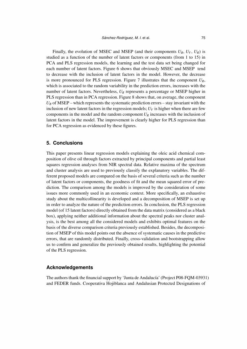
Figure 8: Decomposition of MSEP in PCA and PLS regression as a function of the number of latent factors.
Sanchez-Rodrıguez, M. I. et al. 75
Finally, the evolution of MSEC and MSEP (and their components UB, UV , UR) is
studied as a function of the number of latent factors or components (from 1 to 15) in
PCA and PLS regression models, the learning and the test data set being changed for
each number of latent factors. Figure 6 shows that obviously MSEC and MSEP tend
to decrease with the inclusion of latent factors in the model. However, the decrease
is more pronounced for PLS regression. Figure 7 illustrates that the component UR,
which is associated to the random variability in the prediction errors, increases with the
number of latent factors. Nevertheless, UR represents a percentage or MSEP higher in
PLS regression than in PCA regression. Figure 8 shows that, on average, the component
UB of MSEP – which represents the systematic prediction errors – stay invariant with the
inclusion of new latent factors in the regression models; UV is higher when there are few
components in the model and the random component UR increases with the inclusion of
latent factors in the model. The improvement is clearly higher for PLS regression than
for PCA regression as evidenced by these figures.
5. Conclusions
This paper presents linear regression models explaining the oleic acid chemical com-
position of olive oil through factors extracted by principal components and partial least
squares regression analyses from NIR spectral data. Relative maxima of the spectrum
and cluster analysis are used to previously classify the explanatory variables. The dif-
ferent proposed models are compared on the basis of several criteria such as the number
of latent factors or components, the goodness of fit and the mean squared error of pre-
diction. The comparison among the models is improved by the consideration of some
issues more commonly used in an economic context. More specifically, an exhaustive
study about the multicollinearity is developed and a decomposition of MSEP is set up
in order to analyze the nature of the prediction errors. In conclusion, the PLS regression
model (of 15 latent factors) directly obtained from the data matrix (considered as a black
box), applying neither additional information about the spectral peaks nor cluster anal-
ysis, is the best among all the considered models and exhibits optimal features on the
basis of the diverse comparison criteria previously established. Besides, the decomposi-
tion of MSEP of this model points out the absence of systematic causes in the predictive
errors, that are randomly distributed. Finally, cross-validation and bootstrapping allow
us to confirm and generalize the previously obtained results, highlighting the potential
of the PLS regression.
Acknowledgements
The authors thank the financial support by ‘Junta de Andalucıa’ (Project P08-FQM-03931)
and FEDER funds. Cooperativa Hojiblanca and Andalusian Protected Designations of

76 New insights into evaluation of regression models through a decomposition...
Origin (PDOs) are also gratefully acknowledged for providing the olive oil samples
whereas the access to samples from germplasm bank of Cordoba is also thanked to
IFAPA. Finally, the authors wish to thank Drs Rallo and Moalem for their kind scientific
assistance.
References
Andersen, C. M. and Bro, R. (2010). Variable selection in regression-a tutorial. Journal of Chemometrics,
24, 728–737.
Anderson, M. (2009). A comparison of nine PLS1 algorithms. Journal of Chemometrics, bf 23, 518–529.
Baeten, V., Aparicio, R., Marigheto, N. and Wilson, R. (2003). Manual del aceite de oliva. AMV ediciones,
Mundi-Prensa.
Barker, M. and Rayens, W. (2003). Partial least squares for discrimination. Journal of Chemometrics, 17,
166–173.
Berrueta, L. A., Alonso-Salces, R. M. and Heberger, K. (2007). Supervised pattern recognition in food anal-
ysis. Journal of Chromatography A, 1158, 196–214.
Burnham, K. P. and Anderson, D. R. (2004). Multimodel inference: understanding AIC and BIC in model
selection. Sociological Methods & Research , 33, 261–304.
Climaco-Pinto, R., Barros, A. S., Locquet, N., Schmidtke, L. and Rutledge, D. N. (2009). Improving the de-
tection of significant factors using ANOVA-PCA by selective reduction of residual variability. Ana-
lytica Chimica Acta, 653, 131–142.
Dupuy, N., Duponchel, L., Huvenne, J. P., Sombret, B. and Legrand, P. (1996). Classification of edible fats
and oils by principal component analysis of Fourier transform infrared spectra. Food Chemistry,
57(2), 245–251.
Essi, I. D., Chukuigwe, E. C. and Ojekudo, N. A. (2011). On multicollinearity in nonlinear econometric
models with mis-specified error terms in large samples. Journal of Economics and International
Finance , 3(2), 116–120.
Frank, I. E. and Friedman, J. H. (1993). A statistical view of some chemometrics regression tools. Techno-
metrics, 35(2), 109–135.
Gowen, A. A., Downewy, G., Esquerre, C. and O’Donnell, C. P. (2010). Preventing over-fitting in PLS cal-
ibration models of near-infrared (NIR) spectroscopy data using regression coefficients. Journal of
Chemometrics, 25, 375–381.
Greenberg, E. and Parks, R. P. (1997). A predictive approach to model selection and multicollinearity.
Journal of Applied Econometrics, 12, 67–75.
Guillen, M. D. and Ruiz, A. (2003). Rapid simultaneous determination by proton NMR of unsaturation and
composition of acyl groups in vegetable oils. European Journal of Lipid Science and Technology,
105(11), 688–696.
Guldberg, A., Kaas, E., Deque, M., Yang, S. and Vester Thorsen, S. (2005). Reduction of systematic errors
by empirical model correction: impact on seasonal prediction skill. Tellus, 57(A), 575–588.
Gurdeniz, G. and Ozen, B. (2009). Detection of adulteration of extra-virgin oil by chemometric analysis of
mid-infrared spectral data. Food Chemistry, 116, 519–525.
Kasemsumran, S., Kang, N., Christy, A. and Ozaki, Y. (2005). Partial least squares processing of near-
infrared spectra for discrimination and quantification of adulterated olive oils. Spectroscopy Letters,
38(6), 839–851.
Li, B., Morris, J. and Martin, E. B. (2002). Model selection for partial least squares regression. Chemomet-
rics and Intelligent Laboratory Systems, 64, 79–89.

Sanchez-Rodrıguez, M. I. et al. 77
Lopez-Negrete de la Fuente, R., Garcıa-Munoz, S. and Blegler, L. T. (2010). An efficient nonlinear pro-
gramming strategy for PCA models with incomplete data sets. Journal of Chemometrics, 24, 301–
311.
Mark, H. (1986). Comparative study of calibration methods for near-infrared reflectance analysis using a
nested experimental design. Analytical Chemistry, 58, 2814–2819.
Mark, H. and Workman, J. (1986). Effect of repack on calibrations produced for near-infrared reflectance
analysis. Analytical Chemistry, 58, 1454–1459.
Mevik, B. H. and Cerderkvist, H. R. (2004). Mean squared error of prediction (MSEP) estimates for prin-
cipal component regression (PCR) and partial least squares regression (PLSR). Journal of Chemo-
metrics, 18(9), 422–429.
Mynbaev, K. T. (2011). Regressions with asymptotically collinear regressors. Econometrics Journal, 14,
304–320.
Nelson, P. R. C., MacGregor, J. F. and Taylor, P. A. (2006). The impact of missing measurements on PCA
and PLS prediction and monitoring applications. Chemometrics and Intelligent Laboratory Systems,
80, 1–12.
Ozturk, B., Yalcin, A. and Ozdemir, D. (2010). Determination of olive oil adulteration with vegetable oils
by near infrared spectroscopy coupled with multivariate calibration. Journal of Near Infrared
Spectroscopy, 18, 191–201.
Reinaldo, F. T., Martins, J. P. A. and Ferreira, M. M. C. (2008). Sorting variables using informative vectors
as a strategy for feature selection in multivariate regression. Journal of Chemometrics, 23, 32–48.
Spanos, A. and McGuirk, A. (2002). The problem of near-multicollinearity revisited: erratic vs systematic
volatility. Journal of Econometrics, 108, 365–393.
Vasquez, V. R. and Whiting, W. B. (2006). Accounting for both random errors and systematic errors in
uncertainty propagation analysis of computer models involving experimental measurements with
Monte Carlo methods. Risk Analysis, 25(6), 1669–1680.
Yamagata, T. (2006). The small sample performance of the Wald test in the sample selection model under
the multicollinearity problem. Economics Letters, 93, 75–81.
Yamamoto, H., Yamaji, H., Abe, Y., Harada, K., Waluyo, D., Fukusaki, E., Kondo, A., Ohno, H. and Fukuda,
H. (2009). Dimensionality reduction for metabolome data using PCA, PLS, OPLS, and RFDA with
differential penalties to latent variables. Chemometrics and Intelligent Laboratory Systems, 98, 136–
142.
Zwanenburg, G., Hoefsloot, H. C. J., Westerhuis, J. A., Jansen, J. J. and Smilde, A. K. (2011). ANOVA-
principal component analysis and ANOVA-simultaneous component analysis: a comparison. Journal
of Chemometrics, 25(10), 561–567.

Related Documents