Lecture Notes in Bioinformatics 5167 Edited by S. Istrail, P. Pevzner, and M.Waterman Editorial Board: A. Apostolico S. Brunak M. Gelfand T. Lengauer S. Miyano G. Myers M.-F. Sagot D. Sankoff R. Shamir T. Speed M. Vingron W. Wong Subseries of Lecture Notes in Computer Science

Welcome message from author
This document is posted to help you gain knowledge. Please leave a comment to let me know what you think about it! Share it to your friends and learn new things together.
Transcript

Lecture Notes in Bioinformatics 5167Edited by S. Istrail, P. Pevzner, and M. Waterman
Editorial Board: A. Apostolico S. Brunak M. GelfandT. Lengauer S. Miyano G. Myers M.-F. Sagot D. SankoffR. Shamir T. Speed M. Vingron W. Wong
Subseries of Lecture Notes in Computer Science

Ana L.C. Bazzan Mark CravenNatália F. Martins (Eds.)
Advances inBioinformatics andComputational Biology
Third Brazilian Symposium on Bioinformatics, BSB 2008Santo André, Brazil, August 28-30, 2008Proceedings
13

Series Editors
Sorin Istrail, Brown University, Providence, RI, USAPavel Pevzner, University of California, San Diego, CA, USAMichael Waterman, University of Southern California, Los Angeles, CA, USA
Volume Editors
Ana L.C. BazzanInstituto de Informática, UFRGSPorto Alegre, RS, BrazilE-mail: [email protected]
Mark CravenUniversity of WisconsinMadison, Wisconsin, USAE-mail: [email protected]
Natália F. MartinsEMBRAPA, Recursos Genéticos e BiotecnologiaBrasília, DF, BrazilE-mail: [email protected]
Library of Congress Control Number: 2008932956
CR Subject Classification (1998): H.2.8, F.2.1, I.2, G.2.2, J.2, J.3, E.1
LNCS Sublibrary: SL 8 – Bioinformatics
ISSN 0302-9743ISBN-10 3-540-85556-4 Springer Berlin Heidelberg New YorkISBN-13 978-3-540-85556-9 Springer Berlin Heidelberg New York
This work is subject to copyright. All rights are reserved, whether the whole or part of the material isconcerned, specifically the rights of translation, reprinting, re-use of illustrations, recitation, broadcasting,reproduction on microfilms or in any other way, and storage in data banks. Duplication of this publicationor parts thereof is permitted only under the provisions of the German Copyright Law of September 9, 1965,in its current version, and permission for use must always be obtained from Springer. Violations are liableto prosecution under the German Copyright Law.
Springer is a part of Springer Science+Business Media
springer.com
© Springer-Verlag Berlin Heidelberg 2008Printed in Germany
Typesetting: Camera-ready by author, data conversion by Scientific Publishing Services, Chennai, IndiaPrinted on acid-free paper SPIN: 12453382 06/3180 5 4 3 2 1 0

Preface
The Brazilian Symposium on Bioinformatics (BSB) 2008 was held at SantoAndre (Sao Paulo), Brazil, August 28–30, 2008. BSB 2008 was the third sympo-sium in the BSB series, although BSB was preceded by the Brazilian Workshopon Bioinformatics (WOB). This previous event had three consecutive editions in2002 (Gramado, Rio Grande do Sul), 2003 (Macae, Rio de Janeiro), and 2004(Brasılia, Distrito Federal). The change from workshop to symposium reflectsthe increasing quality and interest behind this meeting.
For BSB 2008, we had 41 submissions: 32 full papers and 9 extended ab-stracts, submitted to two tracks: the main track on Computational Biology andBioinformatics, and the track Applications of Agent Technologies and Multia-gent Systems to Computational Biology. The current proceedings contain 14 fullpapers and 5 extended abstracts that were accepted. These papers and abstractswere carefully refereed and selected by an international Program Committee of35 members, with the help of 13 additional reviewers. We believe that this vol-ume represents a fine contribution to current research in computational biologyand bioinformatics, as well as in molecular biology.
The editors would like to thank: the authors for submitting their work to thissymposium; the Program Committee members as well as additional reviewersfor their support in the review process; the symposium sponsors (see list in thisvolume); and Springer for agreeing to print this volume. We thank especiallythe General and Local Chairs Andre C.P.L.F. de Carvalho (USP/Sao Carlos),Ana Carolina Lorena and Luis Paulo Barbour Scott (UFABC), and Katti Faceli(UFSCar/Sorocaba), as well as Maria Emilia M.T. Walter (UnB) who has givenus valuable hints out of her experience with last year’s proceedings, and the othermembers of the local organization, all from UFABC (Andre Fonseca, ClaudiaBarros Monteiro-Vitorello, Claudio Nogueira de Meneses, Hana Masuda, JiriBorecky, Leonardo Maia, Maria das Gracas Marietto, Mauricio Coutinho, andPaula Homem de Melo). Without their support and hard work this symposiumwould not have been held.
Ana L. C. BazzanMark Craven
Natalia Martins

Organization
BSB 2008 was organized by the CMCC of UFABC (Universidade Federal doABC) in Santo Andre, Brazil.
Executive Committee
Conference Chair Andre C.P.L.F. de CarvalhoUSP/Sao CarlosBrazil
Local Chairs Ana Carolina Lorena (UFABC)Luis Paulo Barbour Scott (UFABC)Katti Faceli (UFSCar/Sorocaba)Brazil
Scientific Program Committee
Program Chairs Ana L. C. BazzanInstituto de Informatica, UFRGSBrazil
Mark CravenUniversity of WisconsinUSA
Natalia F. MartinsEmbrapa Genetic Resources and BiotechnologyBrazil
Program Committee
Aaron Cohen Oregon Health and Science UniversityAdelinde Uhrmacher University of RostockAdelmo Cechin UNISINOSAlba Melo UnBAlberto Apostolico Georgia TechAlexandre Caetano EmbrapaAna Freitas Technical University of LisbonAntonio Miranda FiocruzBernard Maigret edam UHP-NANCYCarlos Eduardo Ferreira USPCarlos H. Inacio Ramos UNICAMPCelia Ralha UnB

VIII Organization
Colin Dewey University of WisconsinDavid Sankoff University of OttawaDaniel Huson Tuebingen UniversityDominique Cellier Universite de RouenEdson Caceres UFMSEmanuela Merelli Universita di CamerinoFernando Von Zuben UNICAMPFrank DiMaio University of WashingtonGad Landau University of HaifaGunnar Klau Freie Universitat BerlinIrene Ong University of Wisconsin MadisonJoao Setubal Virginia TechJose Carlos Mombach UFRGSKarl Tuyls University of MaastrichtGunnar Klau Freie Universitat BerlinMarcilio de Souto UFRGNMarie-Dominique Devignes LORIAMarta Mattoso COPPE/UFRJMelissa Lemos PUC/RioNadia Pisanti University of PisaNalvo Almeida UFMSNey Lemke UNESPOsmar Norberto de Souza PUCRSPaulo Moscato University of NewcastleRyan Lilien University of TorontoSatoru Miyano University of TokyoSiang Song USPStacia Wyman Fred Hutchinson Cancer Research CenterWellington Martins UCG
Sponsors
Brazilian Computer Society (SBC)Fundacao de Apoio a Pesquisa do Estado de Sao Paulo (FAPESP)Conselho Nacional de Desenvolvimento Cientıfico e Tecnologico (CNPq)Coordenacao de Aperfeicoamento de Pessoal de Nıvel Superior (CAPES)Universidade Federal do ABCCLC bioSGI
Table of Contents
Selected Articles
Multi-label Hierarchical Classification of Protein Functions withArtificial Immune Systems . . . . . . . . . . . . . . . . . . . . . . . . . . . . . . . . . . . . . . . . 1
Roberto T. Alves, Myriam R. Delgado, and Alex A. Freitas
Operon Prediction in Bacterial Genomes . . . . . . . . . . . . . . . . . . . . . . . . . . . . 13Matheus B.S. Barros, Simone de L. Martins, and Alexandre Plastino
An Evaluation of the Impact of Side Chain Positioning on the Accuracyof Discrete Models of Protein Structures . . . . . . . . . . . . . . . . . . . . . . . . . . . . 23
Miguel M.F. Bugalho and Arlindo L. Oliveira
Top-Down Hierarchical Ensembles of Classifiers for PredictingG-Protein-Coupled-Receptor Functions . . . . . . . . . . . . . . . . . . . . . . . . . . . . . 35
Eduardo P. Costa, Ana C. Lorena, Andre C.P.L.F. Carvalho, andAlex A. Freitas
A Hybrid Method for the Protein Structure Prediction Problem . . . . . . . 47Marcio Dorn, Ardala Breda, and Osmar Norberto de Souza
Detecting Statistical Covariations of Sequence PhysicochemicalProperties . . . . . . . . . . . . . . . . . . . . . . . . . . . . . . . . . . . . . . . . . . . . . . . . . . . . . . . 57
Moshe A. Gadish and David K.Y. Chiu
Molecular Models to Emulate Confinement Effects on the InternalDynamics of Organophosphorous Hydrolase . . . . . . . . . . . . . . . . . . . . . . . . . 68
Diego E.B. Gomes, Roberto D. Lins, Pedro G. Pascutti,Tjerk P. Straatsma, and Thereza A. Soares
On the Toric Graph as a Tool to Handle the Problem of Sorting byTranspositions . . . . . . . . . . . . . . . . . . . . . . . . . . . . . . . . . . . . . . . . . . . . . . . . . . . 79
Rodrigo de A. Hausen, Luerbio Faria,Celina M.H. de Figueiredo, and Luis Antonio B. Kowada
A Customized Class of Functions for Modeling and Clustering GeneExpression Profiles in Embryonic Stem Cells . . . . . . . . . . . . . . . . . . . . . . . . 92
Shenggang Li, Miguel Andrade-Navarro, and David Sankoff
Extracting Information from Flexible Receptor-Flexible LigandDocking Experiments . . . . . . . . . . . . . . . . . . . . . . . . . . . . . . . . . . . . . . . . . . . . . 104
Karina S. Machado, Evelyn K. Schroeder, Duncan D. Ruiz,Ana Wink, and Osmar Norberto de Souza

X Table of Contents
Transposition Distance Based on the Algebraic Formalism . . . . . . . . . . . . . 115Cleber V.G. Mira, Zanoni Dias, Hederson P. Santos,Guilherme A. Pinto, and Maria Emilia M.T. Walter
Using BioAgents for Supporting Manual Annotation on GenomeSequencing Projects . . . . . . . . . . . . . . . . . . . . . . . . . . . . . . . . . . . . . . . . . . . . . . 127
Celia Ghedini Ralha, Hugo W. Schneider, Lucas O. da Fonseca,Maria Emilia M.T. Walter, and Marcelo M. Brıgido
Application of Genetic Algorithms to the Genetic RegulationProblem . . . . . . . . . . . . . . . . . . . . . . . . . . . . . . . . . . . . . . . . . . . . . . . . . . . . . . . . 140
Maria Fernanda B. Wanderley, Joao C.P. da Silva,Carlos Cristiano H. Borges, and Ana Tereza R. Vasconcelos
Tests for Gene Clusters Satisfying the Generalized AdjacencyCriterion . . . . . . . . . . . . . . . . . . . . . . . . . . . . . . . . . . . . . . . . . . . . . . . . . . . . . . . . 152
Ximing Xu and David Sankoff
Extended Abstracts
Identity Transposon Networks in D. melanogaster . . . . . . . . . . . . . . . . . . . . 161Alcides Castro-e-Silva, Gerald Weber, Romuel F. Machado,Elizabeth F. Wanner, and Renata Guerra-Sa
Prediction of Protein-Protein Binding Hot Spots: A Combination ofClassifiers Approach . . . . . . . . . . . . . . . . . . . . . . . . . . . . . . . . . . . . . . . . . . . . . . 165
Roberto Hiroshi Higa and Clesio Luis Tozzi
AGN Simulation and Validation Model . . . . . . . . . . . . . . . . . . . . . . . . . . . . . 169Fabrıcio M. Lopes, Roberto M. Cesar-Jr., and Luciano da F. Costa
A Practical Evaluation of BioProvider . . . . . . . . . . . . . . . . . . . . . . . . . . . . . . 174Maira Ferreira de Noronha, Sergio Lifschitz, andAntonio Basilio de Miranda
Evaluation of Models for the Recognition of Hadwritten Digits inMedical Forms . . . . . . . . . . . . . . . . . . . . . . . . . . . . . . . . . . . . . . . . . . . . . . . . . . . 178
Willian Zalewski, Huei Diana Lee, Adewole M.J.F. Caetano,Ana C. Lorena, Andre G. Maletzke, Joao Jose Fagundes,Claudio Saddy, Rodrigues Coy, and Feng Chung Wu
Author Index . . . . . . . . . . . . . . . . . . . . . . . . . . . . . . . . . . . . . . . . . . . . . . . . . . 183

A.L.C. Bazzan, M. Craven, and N.F. Martins (Eds.): BSB 2008, LNBI 5167, pp. 1–12, 2008. © Springer-Verlag Berlin Heidelberg 2008
Multi-label Hierarchical Classification of Protein Functions with Artificial Immune Systems
Roberto T. Alves1, Myriam R. Delgado1, and Alex A. Freitas2
1 Programa de Pós-Graduação em Engenharia Elétrica e Informática Industrial, UFTPR Av. Sete de Setembro, 3165, CEP: 80230-901, Curitiba – PR – Brazil
[email protected], [email protected] 2 Computing Laboratory and Centre for BioMedical Informatics, University of Kent,
CT2 7NF, Canterbury, U.K. [email protected]
Abstract. This work proposes two versions of an Artificial Immune System (AIS) - a relatively recent computational intelligence paradigm – for predicting protein functions described in the Gene Ontology (GO). The GO has functional classes (GO terms) specified in the form of a directed acyclic graph, which leads to a very challenging multi-label hierarchical classification problem where a protein can be assigned multiple classes (functions, GO terms) across several levels of the GO's term hierarchy. Hence, the proposed approach, called MHC-AIS (Multi-label Hierarchical Classification with an Artificial Immune System), is a sophisticated classification algorithm tailored to both multi-label and hierarchical classification. The first version of the MHC-AIS builds a global classifier to predict all classes in the application domain, whilst the second version builds a local classifier to predict each class. In both versions of the MHC-AIS the classifier is expressed as a set of IF-THEN classification rules, which have the advantage of representing comprehensible knowledge to biologist users. The two MHC-AIS versions are evaluated on a dataset of DNA-binding and ATPase proteins.
Keywords: Artificial Immune System, Hierarchical and Multi-label Classification, Prediction of Protein Function.
1 Introduction
Artificial Immune Systems (AIS) are one of the most recent natural computing approaches to emerge from computer science. The immune system is a distributed system, capable of constructing and maintaining a dynamical and structural identity, learning to identify previously unseen invaders and remembering what it has learnt. These computational techniques have many potential applications, such as in distributed and adaptive control, machine learning, pattern recognition, fault and anomaly detection, computer security, optimization, and distributed system design [1].
In data mining, ideally the discovered knowledge should be not only accurate, but also comprehensible to the user [2]. This work addresses the multi-label hierarchical classification task of data mining, where the goal is to discover a classification model

2 R.T. Alves, M.R. Delgado, and A.A. Freitas
that predicts more than one class for an example (data instance) across several levels of a class hierarchy, based on the values of the predictor attributes for that example.
Bioinformatics is an inter-disciplinary field, involving the areas of computer science, mathematics, biology, etc. [3]. Among many bioinformatics problems, this paper focuses on the prediction of protein functions from information associated with the protein's primary sequence. As proteins often have multiple functions which are described hierarchically, the use of multi-label hierarchical techniques for the induction of classification models in Bioinformatics is a promising research area. At present, the biological functions that can be performed by proteins are defined in a structured, standardized dictionary of terms called the Gene Ontology (GO) [4].
The AIS algorithms proposed in this paper combine the adaptive global search of the AIS paradigm with advanced concepts and methods of data mining (hierarchical and multi-label classification), in order to solve a challenging bioinformatics problem (protein function prediction – assigns GO terms (classes) to proteins). The AIS presented in this paper discovers knowledge interpretable by the user, in the form of IF-THEN classification rules, unlike other methods proposed in the literature, whose classification model is typically a "black box" which normally does not provide any insight to the user about interesting hidden relationships in the data [5].
2 Multi-label Hierarchical Classification
The classification task of data mining [2] consists of building, in a training phase, a classification model that maps each example ti to a class c ∈ C of the target application domain, with i = 1, 2, ..., n, where n represents the number of examples in the training set.
The majority of classification algorithms cope with problems where each example ti is associated with a single class c ∈ C. These algorithms are called single label. However, some classification problems are considerably more complex because each example ti is associated with a subset of classes C is contained in C of the application domain. Protein function prediction is a typical case of this type of problem, since a protein can perform several biological functions. Algorithms for coping with this kind of problem are called multi-label [6].
There has been a very large amount of research on conventional “flat” (non-hierarchical) classification problems, where the classes to be predicted are not hierarchically organized. However, in some problems the classes are hierarchically organized, which makes the classification problem much more challenging. Problems of this type are known as hierarchical classification problems [7].
In hierarchical classification problems, typically the classes are hierarchically organized in one of the following two forms: as a tree (where each class has at most one parent class) or as a direct acyclic graph (DAG), where each class can have more than one parent. In bioinformatics, two of the most well-known hierarchical structures for classifying protein functions are the enzyme commission hierarchy [8] – organized in the form of a tree and GO [4] – organized in the form of a DAG. The GO consists of a dictionary that defines gene products independent from species. GO actually consists of 3 separate "domains" (very different types of GO terms): molecular function, biological process and cellular component. The GO is structurally organized

Multi-label Hierarchical Classification of Protein Functions 3
in the form of a direct acyclic graph (DAG), where each GO term represents a node of the hierarchical structure.
In hierarchical classification, there are basically two types of classifiers that can be built to cope with the full set of classes to be predicted: local or global classifiers. In local classifiers, for each class c ∈ C a (local) classifier is built to predict whether or not each class c is associated with an example ti. After all classifiers are built, an example ti is submitted to all those classifiers (one for each class) in order to determine which classes are predicted for that example. In global classifiers, a single (global) classifier is built to discriminate among all classes of the application domain and so ti is submitted to a single (potentially very complex) classifier [7].
3 Multi-label Hierarchical Classification with an Artificial Immune System
The immune system as a biological complex adaptive system has provided inspiration for a range of innovative problem solving techniques, including classification tasks [9]. In this paper, the construction of a immune-based learning algorithm is explored whose recognition, distributed, and adaptive nature offer many potential advantages over more traditional models. The AIS algorithm used in this paper is called MHC-AIS (Multi-label Hierarchical Classification with an Artificial Immune System). MHC-AIS is based on the following natural immunology principles: clonal selection, immune network and somatic hypermutation [10,11]. In AIS, antibodies (ab) represent candidate solutions to the target problem, whilst antigens (ag) represent specific instances of the problem. In the context of this work, ab´s represent IF-THEN classification rules and ag´s represent proteins in the training set whose classes have to be predicted by the AIS.
In essence, in the clonal selection theory antibodies are cloned in proportion to their degree of matching ("affinity") to antigens, so that the antibodies which are better in recognizing antigens produce more clones of themselves. The just-generated clones are then subject to a process of somatic hypermutation, where the rate of mutation applied to a clone is inversely proportional to its affinity with the antigens. In computer science terms, the best antibodies are cloned more often and undergo a smaller rate of mutation (have fewer parts of their candidate solution modified) than the worst antibodies. With time this process of clonal selection and hypersomatic mutation leads to better and better candidate solutions to the target problem.
In essence, the theoretical immunology principle of immune networks states that antibodies can recognize not only antigens but also other antibodies. The first kind of recognition stimulates antibody production, but the latter suppresses antibodies, which in computer science terms means a candidate solution tends to suppress other similar candidate solutions, which has the effect of improving the diversity of the search for a (near-)optimal candidate solution.
The training phase of MHC-AIS is performed by two major procedures, called Sequential Covering (SC) and Rule Evolution (RE) procedures. The SC procedure iteratively calls the RE procedure until (almost) all “antigens” (proteins, examples) are covered by the discovered rules. The RE procedure essentially evolves artificial “antibodies” (IF-THEN classification rules) that are used to classify antigens. Then,

4 R.T. Alves, M.R. Delgado, and A.A. Freitas
the best evolved antibody is added to discovered rule set. Each antibody (candidate classification rule) consists of two parts: the rule antecedent (IF part), represented by a vector of conditions (attribute-value pairs), and the rule consequent (THEN part) that represents the classes predicted by the rule. In this work the classes correspond to GO terms denoting protein functions. This work proposes two versions of the MHC-AIS, viz.: local and global versions (more details in the following subsections).
3.1 Global Version
In biological databases a protein is annotated only with its most specific GO term. Given the semantics of the GO’s functional hierarchy, this implicitly means the protein also contains all the functional classes of its ancestral GO terms in the GO's DAG. Hence, in a data preprocessing step, MHC-AIS explicitly assigns to each antigen (protein) both its most specific class(es) (GO term(s)) and all its ancestral classes. MHC-AIS also considers the semantics of the GO’s functional hierarchy when creating classification rules – i.e., it guarantees that, if a rule predicts a given GO term, all its ancestral GO terms are also predicted by the rule.
Fig. 1 shows the high-level pseudocode of the SC procedure.
Input: full protein training set; Output: set of discovered rules; DiscoveredRuleSet = ∅; TrainSet = {set of all protein training examples}; Re-label TrainSet regarding GO's functional class hierarchy; WHILE |TrainSet| > MaxUncovExamp
BestRule = RULE-EVOLUTION(TrainSet); //based on AIS DiscoveredRuleSet = DiscoveredRuleSet U BestRule; updateCoveredClasses(TrainSet, BestRule) removeExamplesWithAllClassesCovered(TrainSet);
END WHLE
Fig. 1. Sequential Covering (SC) procedure
First, it initializes the set of discovered rules with the empty set and initializes the training set with the set of all original training examples. Next, each example in the training set is extended to contain both the original class and all its ancestral classes in the GO hierarchy. Thereafter, the algorithm starts a WHILE loop which, at each iteration, calls the RE procedure. The latter receives, as parameters, the current training set and use AIS algorithm to discover classification rules. The RE procedure returns the best classification rule discovered by the AIS for the current training set. Then the SC procedure adds that rule to the discovered rule set and removes the training examples covered by that rule, as follows. In conventional rule induction algorithms for single-label classification, examples correctly covered by the just discovered rule are removed from the training set. However, in multi-label classification this process is more complex, since different rules and different training examples have different numbers of classes. In the global version of the AIS, the process of example removal works as follows. First, the training examples covered by the just-discovered rule (i.e. examples satisfying the rule's antecedent) are identified.

Multi-label Hierarchical Classification of Protein Functions 5
For each of those examples, its annotated (true) classes which are predicted by the just-discovered rules are marked as covered. As more and more rules are discovered, more and more of the annotated classes of each example will be covered. Only when all the classes of an example are covered that example is removed from the training set. The process of rule discovery terminates when the number of examples in the current training set becomes smaller than a user-defined parameter called MaxUncovExamp. Such procedure avoids the discovery of rules covering too few examples, unlikely to generalize well to the test set [12].
Fig. 2 shows the high-level code of the RE procedure, where rules are obtained by the proposed MHC-AIS. First, the initial population of antibodies ABt=0 is created, where the consequent of each rule contains (initially) all GO classes in the data being mined. At the end of the evolutionary process, the AIS updates the consequent of the discovered rule (to be returned by the RE procedure) to contain only a subset of classes, representing the classes predicted by that rule, as will be explained later.
Input: current TrainSet; Output: the best evolved rule; ABt=0 = Create initial population of antibodies at random; Computefitness(ABt=0,TrainSet); FOR t = 1 to Number of Generations
CL = ProduceClones(ABt-1); CL* = MutateClones(CL); ABt = ABt-1 U CL*; Computefitness(ABt,TrainSet); Suppresion(ABt); Elitism(ABt+1);
END FOR t; Determine the final subset of classes of the best antibody found so far; return(best antibody);
Fig. 2. Rule Evolution (RE) procedure
After its creation, the fitness (quality measure) of each antibody abit=0 of the initial
population is calculated on the training set, where each example represents an antigen agj. The fitness of each abi is computed in two stages. First, a fitness value is associated with each kth-class ck
i contained in the consequent of rule (antibody) abi. The value of this fitness is computed according to the following equation:
( ) i ik k
i i i ik k k k
c cik
c c c c
TP TNfit c
TP FN TN FP= ×
+ + (1)
where:
• TP (true positives) = number of training examples satisfying affinity(abi,agj) ≥ δAF and having the annotated class ck
i. • TN (true negatives) = number of training examples satisfying affinity(abi,agj) < δAF
and not having the annotated class cki.
• FP (false positives) = number of training examples satisfying affinity (abi,agj) ≥ δAF and not having the annotated class ck
i. • FN (false negatives) = number of training examples satisfying affinity (abi,agj) <
δAF and having the annotated class cki.
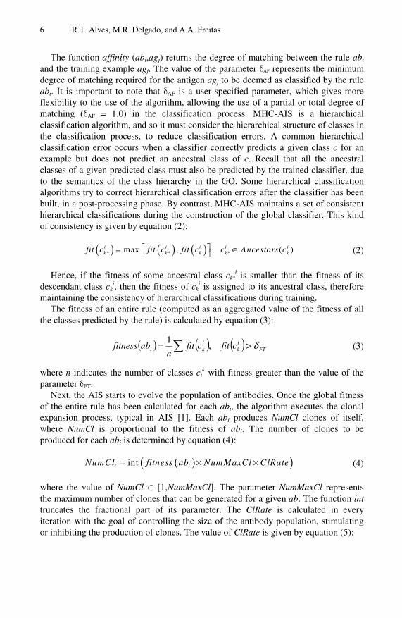
6 R.T. Alves, M.R. Delgado, and A.A. Freitas
The function affinity (abi,agj) returns the degree of matching between the rule abi and the training example agj. The value of the parameter δAF represents the minimum degree of matching required for the antigen agj to be deemed as classified by the rule abi. It is important to note that δAF is a user-specified parameter, which gives more flexibility to the use of the algorithm, allowing the use of a partial or total degree of matching (δAF = 1.0) in the classification process. MHC-AIS is a hierarchical classification algorithm, and so it must consider the hierarchical structure of classes in the classification process, to reduce classification errors. A common hierarchical classification error occurs when a classifier correctly predicts a given class c for an example but does not predict an ancestral class of c. Recall that all the ancestral classes of a given predicted class must also be predicted by the trained classifier, due to the semantics of the class hierarchy in the GO. Some hierarchical classification algorithms try to correct hierarchical classification errors after the classifier has been built, in a post-processing phase. By contrast, MHC-AIS maintains a set of consistent hierarchical classifications during the construction of the global classifier. This kind of consistency is given by equation (2):
( ) ( ) ( )* * *max , , ( )i i i i ik k k k kfit c fit c fit c c Ancestors c⎡ ⎤= ∈⎣ ⎦
(2)
Hence, if the fitness of some ancestral class ck*i is smaller than the fitness of its
descendant class cki, then the fitness of ck
i is assigned to its ancestral class, therefore maintaining the consistency of hierarchical classifications during training.
The fitness of an entire rule (computed as an aggregated value of the fitness of all the classes predicted by the rule) is calculated by equation (3):
( ) ( ) ( ) FTik
iki cfitcfit
nabfitness δ>= ∑ ,
1 (3)
where n indicates the number of classes cik with fitness greater than the value of the
parameter δFT. Next, the AIS starts to evolve the population of antibodies. Once the global fitness
of the entire rule has been calculated for each abi, the algorithm executes the clonal expansion process, typical in AIS [1]. Each abi produces NumCl clones of itself, where NumCl is proportional to the fitness of abi. The number of clones to be produced for each abi is determined by equation (4):
( )( )inti iNumCl fitness ab NumMaxCl ClRate= × × (4)
where the value of NumCl ∈ [1,NumMaxCl]. The parameter NumMaxCl represents the maximum number of clones that can be generated for a given ab. The function int truncates the fractional part of its parameter. The ClRate is calculated in every iteration with the goal of controlling the size of the antibody population, stimulating or inhibiting the production of clones. The value of ClRate is given by equation (5):

Multi-label Hierarchical Classification of Protein Functions 7
if
0 if
1 otherwise
HyperClRate AB nIP
ClRate AB nMaxP
AB nIP
nMaxP nIP
⎧⎪
<⎪⎪= >⎨⎪ ⎛ − ⎞⎪ − ⎜ ⎟⎪ −⎝ ⎠⎩
(5)
where HyperClRate, nIP and nMaxP are specified in the beginning of the execution of the algorithm and indicate, respectively, clonal hyper-expansion rate, initial antibody population size and maximum antibody population size. It is important to emphasize that the parameter nMaxP does not represent the maximum size that the antibody population AB can take during the evolution. Rather, it indicates that, if the size of AB is greater than the value of that parameter, the generation of clones proportional to antibody fitness is turned off. Next, the population CL of clones undergoes a process of somatic hypermutation just on the IF part of the rule. A mutation rate applied to each clone cl is inversely proportional to the fitness of the antibody ab from which the clone was produced. The mutation rate is determined by equation (6):
( ) ( )( )1clMutRate mutMin mutMax mutMin fitness cl= + − × − (6)
where MutMin and MutMax indicate, respectively, the minimum and maximum mutation rates to be applied to a clone cl; and the function fitness(cl) is presented in equation (3). The MutRate represents the probability that each gene (rule condition – IF antecedent) will undergo mutation. The population CL*, which is formed only by clones that underwent some mutation, is then inserted in AB. Other procedures are also applied to AB during the rule evolution procedure: suppression of antibodies and elitism. The suppression procedure, characteristic of AIs based on the immune network theory, removes from ABt similar antibodies. More precisely, if two antibodies abi and abi
* have a similarity degree greater than or equal to the value of δSIM, then, out of those two antibodies, the one with the smallest fitness is removed. The degree of similarity between two antibodies is computed as the number of conditions (attribute-value pairs) in the rule antecedents of both antibodies divided by the number of conditions in the rule antecedent of the antibody with the greatest number of conditions – which produces a measure of antibody similarity normalized in the range from 0 (no rule conditions in common) to 1 (identical rule antecedents). Elitism, a mechanism quite common in evolutionary algorithms [13], selects the antibody with the best fitness to be included in the next-iteration population ABt+1.
During the rule evolution procedure all the classes occurring in the data being mined are represented in the consequent. The choice of the final subset of classes to be assigned to the consequent of the best discovered rule is given by equation (7):
PC = U ck ∈ C | fit(ck) > δFT (7)
where PC represents the set of classes predicted by the best discovered rule whose fitness value is greater than δFT.

8 R.T. Alves, M.R. Delgado, and A.A. Freitas
3.2 Local Version
Like the global MHC-AIS, the local MHC-AIS consists of the SC (Fig. 3) and RE procedures, but with some differences. In the local version, the SC procedure labels the training examples as positive or negative. Positive examples represent examples associated with the class of the current node of the GO’s DAG (a classifier is trained for each node of the GO’s DAG), denoted class Y, whilst examples that do not have the class Y are labeled as negative examples. MHC-AIS is an algorithm for constructing hierarchical classifiers, and therefore the hierarchical structure has to be coped with like in the global version. Hence, all training examples labeled with any descendant class or ancestor class of the current class Y are labeled as positive class. Concerning the latter type of positive examples, it is often the case that, when a hierarchical classifier is being built, examples annotated with an ancestor class of the current class Y are removed, since they are considered as ambiguous – they do not have an annotation suggesting that they have class Y, but maybe they actually have class Y, which was not annotated yet simply due to the lack of evidence for its presence (note that “absence of evidence is different from evidence of absence”). However, in this work we use examples with an annotated class that is an ancestral of the current class Y in order to increase the number of positive examples and so hopefully increase the predictive accuracy of the algorithm.
Input: full training set; Output: set of discovered rules; DiscoveredRuleSet = ;FOR EACH class c
TrainSet = {set of all training examples}; WHILE |TrainSet| > MaxUncovExamp
BestRule = RULE-EVOLUTION(TrainSet, class c);//based on AIS DiscoveredRuleSet=DiscoveredRuleSet U BestRule;
TrainSet = TrainSet – {examp. correctly covered by BestRule}; END WHILE; END FOR EACH class;
Fig. 3. Sequential Covering (SC) procedure for Local Version
In this local version, MHC-AIS first discovers as many classification rules as necessary in order to cover the positive examples. Next, the algorithm discovers as many rules as necessary to cover the negative examples. Every time that a given rule is discovered, all the examples correctly covered by that rule (i.e. examples satisfying the conditions in the rule antecedent and having the class predicted by the rule consequent) are removed from the current training set, as usual in rule induction algorithms. This iterative process of rule discovery and removal of training examples is repeated until the number of examples in the current training set becomes smaller than a user-defined threshold MaxUncovExamp.
The other procedures of the local MHC-AIS are the same as in the global version of the algorithm, described in the previous subsection.
Multi-label Hierarchical Classification of Protein Functions 9
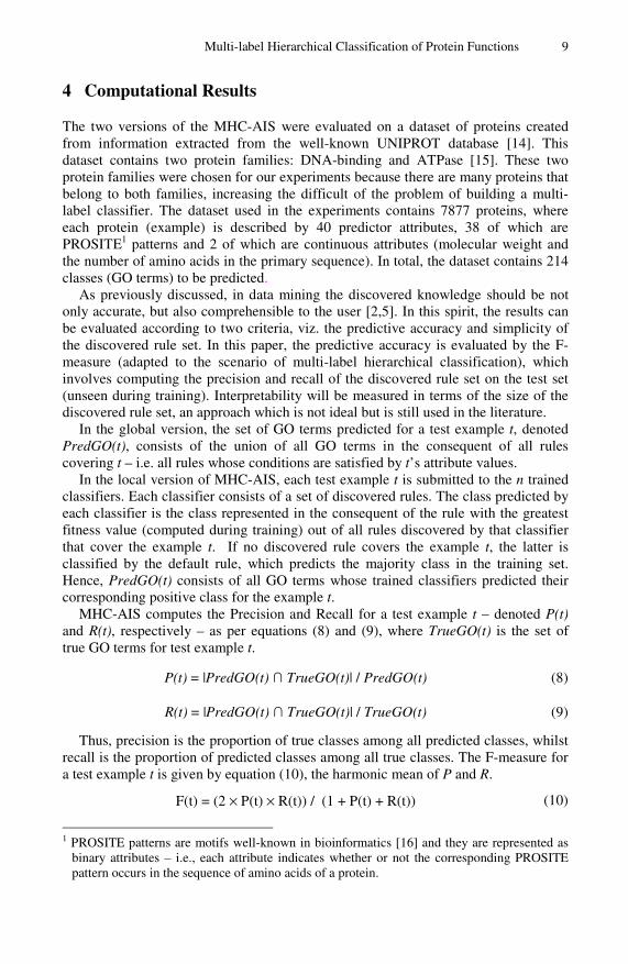
4 Computational Results
The two versions of the MHC-AIS were evaluated on a dataset of proteins created from information extracted from the well-known UNIPROT database [14]. This dataset contains two protein families: DNA-binding and ATPase [15]. These two protein families were chosen for our experiments because there are many proteins that belong to both families, increasing the difficult of the problem of building a multi-label classifier. The dataset used in the experiments contains 7877 proteins, where each protein (example) is described by 40 predictor attributes, 38 of which are PROSITE1 patterns and 2 of which are continuous attributes (molecular weight and the number of amino acids in the primary sequence). In total, the dataset contains 214 classes (GO terms) to be predicted.
As previously discussed, in data mining the discovered knowledge should be not only accurate, but also comprehensible to the user [2,5]. In this spirit, the results can be evaluated according to two criteria, viz. the predictive accuracy and simplicity of the discovered rule set. In this paper, the predictive accuracy is evaluated by the F-measure (adapted to the scenario of multi-label hierarchical classification), which involves computing the precision and recall of the discovered rule set on the test set (unseen during training). Interpretability will be measured in terms of the size of the discovered rule set, an approach which is not ideal but is still used in the literature.
In the global version, the set of GO terms predicted for a test example t, denoted PredGO(t), consists of the union of all GO terms in the consequent of all rules covering t – i.e. all rules whose conditions are satisfied by t’s attribute values.
In the local version of MHC-AIS, each test example t is submitted to the n trained classifiers. Each classifier consists of a set of discovered rules. The class predicted by each classifier is the class represented in the consequent of the rule with the greatest fitness value (computed during training) out of all rules discovered by that classifier that cover the example t. If no discovered rule covers the example t, the latter is classified by the default rule, which predicts the majority class in the training set. Hence, PredGO(t) consists of all GO terms whose trained classifiers predicted their corresponding positive class for the example t.
MHC-AIS computes the Precision and Recall for a test example t – denoted P(t) and R(t), respectively – as per equations (8) and (9), where TrueGO(t) is the set of true GO terms for test example t.
P(t) = |PredGO(t) ∩ TrueGO(t)| / PredGO(t) (8)
R(t) = |PredGO(t) ∩ TrueGO(t)| / TrueGO(t) (9)
Thus, precision is the proportion of true classes among all predicted classes, whilst recall is the proportion of predicted classes among all true classes. The F-measure for a test example t is given by equation (10), the harmonic mean of P and R.
F(t) = (2 × P(t) × R(t)) / (1 + P(t) + R(t)) (10)
1 PROSITE patterns are motifs well-known in bioinformatics [16] and they are represented as
binary attributes – i.e., each attribute indicates whether or not the corresponding PROSITE pattern occurs in the sequence of amino acids of a protein.

10 R.T. Alves, M.R. Delgado, and A.A. Freitas
Finally, once P(t) and R(t) have been computed for each test example t, the system computes the overall F-measure over the entire test set T by equation (11), where |T| denotes the cardinality of the test set T.
Predictive Accuracy = F(T) = (Σt∈T F(t)) / |T| (11)
Table 1 shows the predictive accuracy for precision, recall and F-measure for global and local version. The numbers after the "±" symbol represent the standard deviations associated with a well-known 10-fold cross-validation procedure [2]. In the columns F-measure, the best result (out of both version of MHC-AIS) is shown in bold. The results presented in Table 1 consider different affinity (matching) thresholds for both versions of MHC-AIS, to evaluate the predictive performance of the algorithms using partial matching (δAF < 1.0) or total matching (δAF = 1.0).
Table 1. Predictive accuracy (%) of MHC-AIS versions on the used protein data set
Global Version Local Version Affinity Threshold Precision Recall F-Measure Precision Recall F-Measure
0.8 45.93±2.71 98.23±0.61 58.35±2.23 80.58±1.01 44.65±1.59 55.65±1.45 0.9 50.79±3.18 92.86±3.76 58.34±2.86 75.61±1.12 52.57±2.35 59.75±1.77 1.0 28.91±1.31 99.50±0.12 42.84±1.37 58.56±1.01 69.91±1.13 61.37±0.82
Table 1 shows that the global MHC-AIS performed worst (according to the F-measure) when using total matching. Note that the global MHC-AIS obtained the worst results for the precision measure with all affinity threshold values. By contrast, the global MHC-AIS obtained very good recall values with all affinity thresholds. This performance behavior of global MHC-AIS indicates that the trained global classifier has a bias favoring the prediction of a large number of classes, mainly because the set of classes predicted for a test example consists of the union of all classes in the consequents of all rules covering that example - regardless of the fitness of the individual rules in question and the fact that the predictions of some of those rules might be inconsistent with each other. This tends to predict more classes than the actual number of true classes for a given test example, which tends to increase recall but reduce precision (given the definition of these terms).
In both cases of MHC-AIS, as the value of the affinity threshold δAF increases the value of precision is reduced, showing a disadvantage in the use of total matching. As expected, due to the trade-off between precision and recall, the local version of the algorithm had the opposite performance behavior in the case of recall, where the largest value was obtained with total matching.
Table 2. Simplicity of the discovered rule set of MHC-AIS versions
Global Version Local Version Threshold Affinity #rules #Conditions #rules #Conditions
0.8 63.90±1,59 1164,30±28.20 788.00±3.68 2901.30±42.83 0.9 58.09±3.08 1066.60±53.39 1016.80 ±8.09 4829.80±67.44 1.0 79.90±1.83 1361.00±41.16 1232.90±16.07 7069.53±18298

Multi-label Hierarchical Classification of Protein Functions 11
Table 2 shows the results of both local and global versions of MHC-AIS with respect to the simplicity (interpretability) of the discovered rule set. This simplicity was measured by the number of discovered rules and total number of rule conditions (in all rules). The averages were computed over 10-fold cross-validation.
Note that, as shown in Table 2, the global MHC-AIS obtained much better results concerning rule set simplicity than the local MHC-AIS, in all experiments. This advantage of the global MHC-AIS is probably due to the fact that, by building a single set of rules predicting all classes in a single run of the algorithm, the algorithm can avoid the need for discovering redundant rules covering the same set of true classes for some examples. In particular, when the local version discovers rules predicting the “negative” class at each node of the GO’s DAG, it should be noted that those rules predicting the negative class tend to be redundant with respect to rules predicting positive classes in other nodes of the GO’s DAG, since some of the negative class examples for a given GO node will inevitably be positive class examples in another GO node. An example of a rule discovered rule by global MHC-AIS in the used data set is presented below:
IF (PS00676 == 1) and (PS00390 == 1) and (MOLECULAR_WEIGHT < 29353) then (5488, 5515, 51087)
The biological interpretation of this rule is: if a protein presents “Sigma-54 interaction domain signatures and profile” and “Sodium and potassium ATPases beta subunits signatures” signatures and “molecular weight is less than 29353” then the predicted classes (biological functions) are: “binding” (5488) and “protein binding” (5515) and “chaperone binding” (51087). Note that the GO hierarchy was considered, i.e. the true hierarchical path is 5488 → 5515 → 51087 (from shallower to deeper nodes).
5 Conclusion and Future Work
This work described an artificial immune system (AIS)-based rule induction algorithm to the prediction of protein function. The paper proposed two versions of the AIS algorithm, a global version, where a single global classifier is built predicting all classes of the application domain; and a local version, where a local classifier is built for each node of the GO class hierarchy. Both versions have the advantage of discovering IF-THEN classification rules, constituting a type of knowledge representation that can, in principle, be easily interpretable by biologist users. The global and local versions of the AIS have different (roughly dual) advantages and disadvantages with respect to predictive accuracy, but the global version at least has the advantage of discovering much simpler (smaller) rule sets.
Future work involves: (a) comparing the predictive performance of both versions of the AIS with other classification algorithms designed for hierarchical classification (e.g. [17]); (b) investigating new criteria for selecting, out of all classes in the consequent of the rules covering a test example in the global approach, which classes should be actually predicted for the test example; (c) incorporating an explicit mechanism during the training phase to improve the rules´ interpretability (d) analyzing the biological relevance of the discovered rules; and (e) evaluating the proposed AIS in datasets of other protein families and other types of predictor attributes.

12 R.T. Alves, M.R. Delgado, and A.A. Freitas
References
1. De Castro, L.N., Timmis, J.: Artificial Immune Systems: A New Computational Intelligence Approach. Springer, Berlin (2002)
2. Witten, I.H., Frank, E.: Data Mining: Practical Machine Learning Tools and Techniques, 2nd edn. Morgan Kaufmann, San Mateo (2005)
3. Fogel, G.B., Corne, D.W.: Evolutionary Computation in Bioinformatics. Morgan Kaufmann Publishers, San Franciso (2003)
4. The Gene Ontology Consortium. The Gene Ontology (GO) Database and Informatics Resource. Nucleic Acids Research 32(1), 258–261 (2004)
5. Freitas, A.A.: Data Mining and Knowledge Discovery with Evolutionary Algorithms. Springer, Berlin (2002)
6. Tsoumakas, G., Katakis, I.: Multi-Label Classification: An Overview. International Journal of Data Warehousing and Mining 3(3), 1–13 (2007)
7. Sun, A., Lim, E.-P., Ng, W.-K.: Performance Measurement Framework for Hierarchical Text Classification. Journal of the American Society for Information Science and Technology 54(11), 1014–1028 (2003)
8. E. Nomenclature, of the IUPAC-IUB. American Elsevier Pub. Co., New York, NY 104 (1972)
9. Freitas, A.A., Timmis, T.: Revisiting the foundations of artificial immune systems for data mining. IEEE Trans. on Evolutionary Computation 11(4), 521–540 (2007)
10. Ada, G.L., Nossal, G.V.: The Clonal Selection Theory. Scientific American 257, 50–57 (1987)
11. Jerne, N.K.: Towards a Network Theory of Immune System. Ann. Immunol (Inst. Pasteur) 125C, 373–389 (1974)
12. Alves, R.T., Delgado, M.R., Lopes, H.S., Freitas, A.A.: An artificial immune system for fuzzy-rule induction in data mining. In: Yao, X., Burke, E.K., Lozano, J.A., Smith, J., Merelo-Guervós, J.J., Bullinaria, J.A., Rowe, J.E., Tiňo, P., Kabán, A., Schwefel, H.-P. (eds.) PPSN 2004. LNCS, vol. 3242, pp. 1011–1020. Springer, Heidelberg (2004)
13. Goldberg, D.E.: Genetic Algorithms in Search Optimization and Machine Learning. Addison-Wesley, Reading (1989)
14. The UniProt Consortium. The Universal Protein Resource (UniProt). Nucleic Acids Res. 35, D193–D197 (2007)
15. Alberts, B., Johnson, A., Lewis, J., Raff, M., Roberts, K., Water, P.: Molecular Biology of the Cell, 4th edn. Garland Science, New York (2002)
16. Hulo, N., Bairoch, A., Bulliard, V., Cerutti, L., De Castro, E., Langendijk-Genevaux, P.S., Pagni, M., Sigrist, C.J.A.: The PROSITE Database. Nucleic Acids Res. 34, D227–D230 (2006)
17. Wolstencroft, K., Lord, P.W., Tabernero, P., Brass, P., Stevens, R.: Protein classification using ontology classification. Bioinformatics 22, 530–538 (2006)

Operon Prediction in Bacterial Genomes�
Matheus B.S. Barros, Simone de L. Martins, and Alexandre Plastino
Departamento de Ciencia da Computacao – Universidade Federal Fluminense (UFF)24210-240 – Niteroi – RJ – Brasil
[email protected], {simone,plastino}@dcc.ic.uff.br
Abstract. Operons are sets of adjacent genes that encode proteins withrelated metabolic functions. Operon prediction may be useful forunderstanding the systems of regulation and for genome annotation. Inthis work, we present an extension of the PROCSIMO tool to allowthe operon prediction in bacterial genomes based on the similarity eval-uation between pairs of genes. Computational experiments were madeto validate this new functionality. With the use of this tool, we expectto enlarge the number of known operons in bacterial organisms.
1 Introduction
The genes of bacterial genomes are organized in operons which are sets ofgenes transcribed into a single mRNA sequence. Operons form the fundamentaltranscriptional units within a bacterial genome, so defining these structures mayhelp in examining transcriptional regulation. In addition, operons often containgenes that are functionally related and required by the cell for a certain processor pathway and, thus, they are highly predictive of biological networks. For thesereasons, identifying the genes that are grouped together into operons may en-hance our knowledge of gene regulation and function, and such information isan important addition to genome annotation [1,2,3].
The PROCSIMO tool [4] was developed to identify similarity betweenoperons. The main contribution of this work is to add a new functionality tothis tool, which enables the operon prediction in new sequenced genomes.
A variety of prediction algorithms has been developed in recent years. Cravenet al. [5] present an approach which uses machine learning methods to inducepredictive models from a variety of data types including sequence data, geneexpression data, and functional annotations associated with genes. The learnedmodels are used to individually predict promoters, terminators and operonsthemselves and a dynamic programming method uses these predictions to mapevery known and putative gene in a given genome into its most probable operon.This method is more suitable to highly characterized genomes, such as the E. coliK-12 genome, because it needs lots of input data.
Another method, proposed in [2], is based on finding gene clusters in whichgene order and orientation are conserved in two or more genomes. This approach
� Work sponsored by CNPq.
A.L.C. Bazzan, M. Craven, and N.F. Martins (Eds.): BSB 2008, LNBI 5167, pp. 13–22, 2008.c© Springer-Verlag Berlin Heidelberg 2008
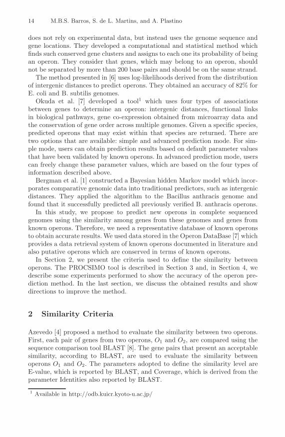
14 M.B.S. Barros, S. de L. Martins, and A. Plastino
does not rely on experimental data, but instead uses the genome sequence andgene locations. They developed a computational and statistical method whichfinds such conserved gene clusters and assigns to each one its probability of beingan operon. They consider that genes, which may belong to an operon, shouldnot be separated by more than 200 base pairs and should be on the same strand.
The method presented in [6] uses log-likelihoods derived from the distributionof intergenic distances to predict operons. They obtained an accuracy of 82% forE. coli and B. subtilis genomes.
Okuda et al. [7] developed a tool1 which uses four types of associationsbetween genes to determine an operon: intergenic distances, functional linksin biological pathways, gene co-expression obtained from microarray data andthe conservation of gene order across multiple genomes. Given a specific species,predicted operons that may exist within that species are returned. There aretwo options that are available: simple and advanced prediction mode. For sim-ple mode, users can obtain prediction results based on default parameter valuesthat have been validated by known operons. In advanced prediction mode, userscan freely change these parameter values, which are based on the four types ofinformation described above.
Bergman et al. [1] constructed a Bayesian hidden Markov model which incor-porates comparative genomic data into traditional predictors, such as intergenicdistances. They applied the algorithm to the Bacillus anthracis genome andfound that it successfully predicted all previously verified B. anthracis operons.
In this study, we propose to predict new operons in complete sequencedgenomes using the similarity among genes from these genomes and genes fromknown operons. Therefore, we need a representative database of known operonsto obtain accurate results. We used data stored in the Operon DataBase [7] whichprovides a data retrieval system of known operons documented in literature andalso putative operons which are conserved in terms of known operons.
In Section 2, we present the criteria used to define the similarity betweenoperons. The PROCSIMO tool is described in Section 3 and, in Section 4, wedescribe some experiments performed to show the accuracy of the operon pre-diction method. In the last section, we discuss the obtained results and showdirections to improve the method.
2 Similarity Criteria
Azevedo [4] proposed a method to evaluate the similarity between two operons.First, each pair of genes from two operons, O1 and O2, are compared using thesequence comparison tool BLAST [8]. The gene pairs that present an acceptablesimilarity, according to BLAST, are used to evaluate the similarity betweenoperons O1 and O2. The parameters adopted to define the similarity level areE-value, which is reported by BLAST, and Coverage, which is derived from theparameter Identities also reported by BLAST.
1 Available in http://odb.kuicr.kyoto-u.ac.jp/

Operon Prediction in Bacterial Genomes 15
The E-value reported by BLAST, between two genes, G1 and G2, is a param-eter that describes the number of hits one can expect to see by chance whensearching genes of a particular size [9]. BLAST(G1,G2) represents this value andlower values indicates that the number of hits is more significant.
The Coverage, represented by Cover(G1,G2) indicates the pairwise alignmentpercentage, and has values in the interval [0 , Identities
number bases(G2) × 100 ], wherenumber bases(G1) ≤ number bases(G2) and Identities is a value reported byBLAST, which represents the extent to which two sequences are invariant.
For evaluating the similarity between operons O1 and O2, based on all pairs ofgenes that were considered similar according to limit values for E-value (emax)and Coverage (cmin), Azevedo [4] proposed the following similarity criteria:
– Number of Similar Genes (NSG). Two operons O1 and O2 present similaritylevel k, according to criterion NSG, if there are k similar gene pairs (G1,G2),where G1 is a gene from O1 and G2 is a gene from O2 or its inversion. Thesame gene or its inversion must not appear in more than one of these k genepairs.
– Average E-value (AEV). The similarity level r among two operons O1 andO2, according to criterion AEV, is defined as the average of the E-values ofthe k similar gene pairs.
– Inversions Number (IN). Consider that the k similar gene pairs (G11,G21),(G12,G22), ..., (G1k,G2k) are organized in such a way that (G1i,G2i) precedes(G1j ,G2j) if and only if G1i appears before G1j in O1. In this way, the genesfrom O2 which belong to the k pairs do not have to be in the same orderand direction as they are in operon O2. O1 and O2 present similarity levels, according to criteria IN, if s inversion operations should be made in chainG21G22. . . G2k to obtain the same order and direction in which they are inO2.
– Size Difference (SD). The similarity level d between operons O1 and O2,according to criteria SD, is defined as the modulus of the difference betweenthe size of operons O1 and O2, where the size of an operon is considered asthe number of its bases.
– Difference of Intergenic Regions (DIR). The similarity level u between oper-ons O1 and O2, according to criteria DIR, is defined as the difference modulusbetween the average intergenic regions of operons O1 and O2, where an in-tergenic region of an operon is considered as the number of its bases locatedbetween a pair of operon genes.
3 The PROCSIMO Tool
In this Section, we present the functionality of the PROCSIMO tool [4] anddescribe how the operon prediction function was added to this tool.
3.1 The Tool Functionality
The PROCSIMO tool, as defined in [4], was developed to identify operons,stored in a database, which are similar to an input operon. We added a new

16 M.B.S. Barros, S. de L. Martins, and A. Plastino
functionality to this tool, which predict operons in complete genomes, using thesame similarity criteria described in the previous section.
The tool has two modules: the Search Module and the Consult Module. Thefirst one implements the basic tool functions: the similarity search among operonsstored in a database and an input operon, and the operon prediction in completegenomes. The second one allows the user to access information about the operonsstored in the database, and the genes which compose these operons.
The present tool database stores operons extracted from the Operon Database[7], and the base sequences of the operon genes were obtained from GenBank [10].The tool administrator may include, exclude or update any database component(organism, operon or gene).
The tool was projected to enable its access via Internet using a navigator,such as Mozilla Firefox. We use the following free software tools: PERL 5.0 [11],the database server MySQL 5.0 Server [12] and the webserver Apache 2.0 [13].
3.2 Operon Prediction
The main contribution of this work is to add the operon prediction functional-ity to the PROCSIMO tool. This new functionality aims to predict operons inan input complete genome by comparing the similarity among genes from thecomplete genome to genes from the operon database.
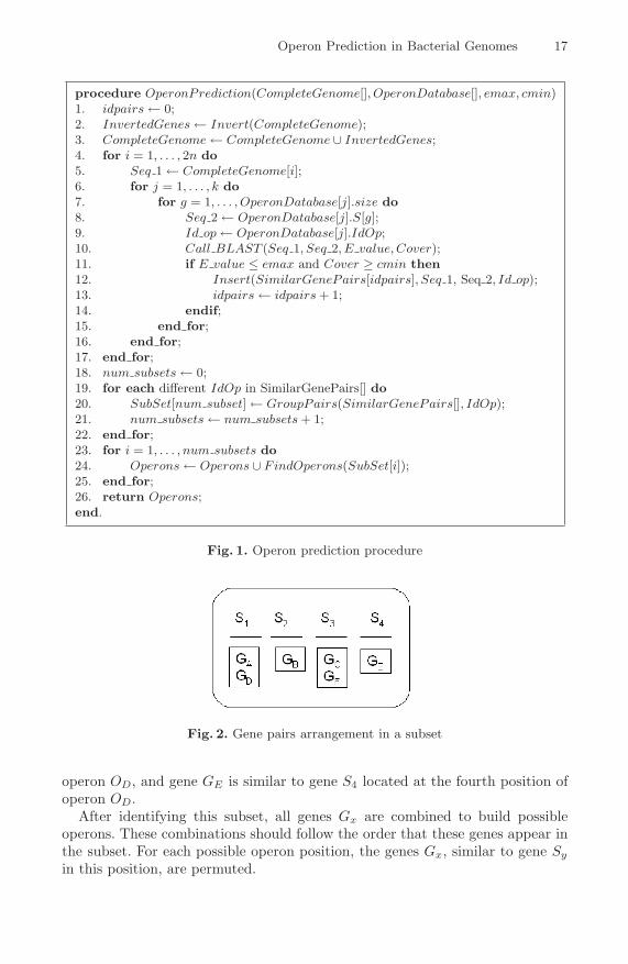
The pseudo-code in Figure 1 illustrates the main steps of the developed pro-cedure to implement this new functionality.
This procedure uses as input data: CompleteGenome[], which contains the ngene sequences of the complete genome; OperonDatabase[], which contains thegene sequence S[], the number of genes in S[] (size), and an identifier (IdOp)for each of the k operons; values emax and cmin, defined by the user and usedto filter the genes from the complete genome that may be in an operon.
From line 4 to line 17, all genes from CompleteGenome[] are pairwise com-pared to all genes from OperonDatabase[] using BLAST. The pairs which presentE value > emax and Cover < cmin are discarded. The other pairs are insertedin SimilarGenePairs. From line 18 to line 22, the pairs from SimilarGenePairsare grouped in subsets according to the operon identifier. Then, from line 23 to25, for each subset, all genes from the complete genome are combined in orderto find possible operons.
To exemplify this procedure execution, consider an operon OD from thedatabase composed of genes S1S2S3S4 and an input complete genome CGI com-posed of genes GAGBGCGDGEGF . After making a BLAST pairwise compar-ison of (GA, S1), . . . , (GA, S4), . . . , (GF , S4), the gene pairs (GA, S1), (GD, S1),(GB , S2), (GC , S3), (GF , S3), (GE , S4) are considered similar according to valuesemax and cmin. As all genes Si belong to operon OD, these pairs are groupedin one subset as illustrated in Figure 2. Genes GA and GD are similar to geneS1, which is located at the first position of database operon OD. Gene GB issimilar to gene S2 located at the second position of operon OD. Genes GC andGF are similar to gene S3, which is located at the third position of database
Operon Prediction in Bacterial Genomes 17
procedure OperonPrediction(CompleteGenome[], OperonDatabase[], emax, cmin)1. idpairs ← 0;2. InvertedGenes ← Invert(CompleteGenome);3. CompleteGenome ← CompleteGenome ∪ InvertedGenes;4. for i = 1, . . . , 2n do5. Seq 1 ← CompleteGenome[i];6. for j = 1, . . . , k do7. for g = 1, . . . , OperonDatabase[j].size do8. Seq 2 ← OperonDatabase[j].S[g];9. Id op ← OperonDatabase[j].IdOp;10. Call BLAST (Seq 1, Seq 2, E value, Cover);11. if E value ≤ emax and Cover ≥ cmin then12. Insert(SimilarGenePairs[idpairs], Seq 1, Seq 2, Id op);13. idpairs ← idpairs + 1;14. endif;15. end for;16. end for;17. end for;18. num subsets ← 0;19. for each different IdOp in SimilarGenePairs[] do20. SubSet[num subset] ← GroupPairs(SimilarGenePairs[], IdOp);21. num subsets ← num subsets + 1;22. end for;23. for i = 1, . . . , num subsets do24. Operons ← Operons ∪ FindOperons(SubSet[i]);25. end for;26. return Operons;end.
Fig. 1. Operon prediction procedure
Fig. 2. Gene pairs arrangement in a subset
operon OD, and gene GE is similar to gene S4 located at the fourth position ofoperon OD.
After identifying this subset, all genes Gx are combined to build possibleoperons. These combinations should follow the order that these genes appear inthe subset. For each possible operon position, the genes Gx, similar to gene Sy
in this position, are permuted.

18 M.B.S. Barros, S. de L. Martins, and A. Plastino
Fig. 3. Predicted operons
Fig. 4. Operon prediction for organism Salmonella typhy Ty2
Figure 3 shows all possible combinations for the subset presented in Figure 2.For this example, we have four predicted operons.
After that, for each predicted operon and its similar database operon, the toolevaluates the values associated to each similarity criterion, and the results areshown according to a precedence order defined by the user.
Figure 4 illustrates the results obtained for predicting operons of organismSalmonella typhy Ty2. In practice, many operons were found, so we show onlythree of these operons. For this example, values 0.5 and 70% were used for emaxand cmin and the precedence criteria order for visualizing results is: NSG, AEV,IN, SD and DIR.
The first line of Figure 4 indicates that genes t2139, t2140, t2141, t2142,t2143 and t2144 of Salmonella typhy Ty2 are candidates to compose an operon.These genes were similar to the second, third, fourth, fifth, sixth and seventhgenes of the putative 11 operon of Shigella flexneri 2a 2457T. The first geneof the putative 11 operon was not similar to any gene from the input completegenome and this is represented by ‘X’. The columns AEV and IN present thevalue 0, which indicates a great similarity between this predicted operon andthe putative 11 operon according to these criteria. Value 0 in column IN alsoindicates that there are no changes in order or direction among the genes of thesetwo operons. The value 13759(putative 11 >) in column SD indicates that theoperon putative 11has 13759 more bases than the predicted operon. The value2693 in column DIR indicates the average intergenic regions difference betweenthe two operons.

Operon Prediction in Bacterial Genomes 19
The second line indicates that genes t4434, t4435, t4436, t4437, t4438 andt4439 compose a predicted operon and are similar to all genes of the operonulaABCDEF. The value 0 in columns AEV and IN indicates a maximum simi-larity degree for these two criteria. The value 32(ulaABCDEF <) in column SDindicates that operon ulaABCDEF has 32 less bases than the predicted operon.Value 46 in column DIR indicates the average intergenic region difference be-tween the two operons.
The third line indicates that genes t3774, t3775, t3776, t3777 and t3778 ofSalmonella typhy Ty2 compose another predicted operon. The genes of thisoperon are all similar to genes of operon spoT from Escherichia coli k12. Thevalue 0 in column AEV indicates maximum level of similarity according to thiscriterion. The value 5 in column IN indicates that five inversion operations shouldbe made in the chain of the predicted operon, so that its genes present the sameorder and direction of genes from operon spoT. The value 63(spoT <) indicatesthat operon spoT has 63 less bases than the predicted operon and the value 1indicates a significant level of similarity, according to DIR criterion.
4 Experimental Results
In this section, we present results obtained from experiments executed to vali-date the new functionality of PROCSIMO tool developed to predict operons incomplete sequenced genomes. All base gene sequences and operons stored in thetool database were obtained from GenBank [10] and Operon DataBase [7].
For all experiments, the tool database stores genes and operons from thefollowing 16 organisms: Escherichia coli K12, Escherichia coli O157:H7 Sakai,Acinetobacter sp. ADP1, Haemophilus influenzae KW20 Rd, Legionella pneu-mophila Paris, Pseudomonas putida KT2440, Shewanella oneidensis MR-1,Shigella flexneri 2a 2457T, Vibrio parahaemolyticus RIMD 2210633, Xylella fas-tidiosa 9a5c, Methylococcus capsulatus Bath, Photorhabdus luminescens TTO1,Yersinia pestis KIM, Erwinia carotovora, Legionella pneumophila Philadelphia1 and Vibrio vulnificus CMCP6.
The criteria similarity order used to present the results is: (1) Number ofSimilar Genes (NSG) , (2) Average E-value (AEV), (3) Inversions Number (IN),(4) Size Difference (SD) and (5) Difference of Intergenic Regions (DIR).
In Sections 4.1, 4.2 and 4.3, we present obtained results of operon predictionfor organisms Salmonella typhy Ty2, Legionella pneumophila Lens e Escherichiacoli O157:H7 Sakai.
4.1 Salmonella Typhy Ty2
In this experiment, the complete genome from Salmonella typhi Ty2 is the inputdata to PROCSIMO tool. The aim is to verify the number of operons thatPROCSIMO can correctly identify.

20 M.B.S. Barros, S. de L. Martins, and A. Plastino
Fig. 5. Number of predicted operons for Salmonella typhy Ty2
This experiment was done using several values for emax: 1, 0.5, 5e-023,5e-050, 5e-070, 5e-100, 5e-200, 5e-300 and 0, and three different values for cmin:50%, 70% and 100%. Thus, combining these values, 27 queries were submittedto PROCSIMO. According to Operon Database [7], Salmonella typhi Ty2 has191 operons.
Figure 5 shows the obtained results. Each curve represents the queriesexecuted for the same cmin value and different emax values. Each pointindicates the number of predicted operons. For example, for query using emaxequal to 1 and cmin equal to 50%, the tool identified 459 operons for the organ-ism Salmonella typhy Ty2.
To verify the tool accuracy, we evaluated the number of the predicted operonswhich are indeed real operons from Salmonella typhy Ty2. Figure 6 illustrates theobtained results. Using emax = 1 and cmin = 50%, 459 operons were predictedby the tool, among which 98 are real operons of Salmonella typhy Ty2.
We observe in Figures 5 and 6 that, as we decrease emax and increase cmin,the number of predicted operons and the number of real operons returned bythe tool decrease, because these parameter values make queries more restrictive.
To verify the efficiency of this tool compared to another operon predictiontool, we used the tool proposed in [7], which is available via Internet, for thesame input organism Salmonella typhy Ty2. This tool predicted 857 operons, insimple mode execution, among which only 71 were real operons.
Thus, we can conclude that, for this experiment, PROCSIMO tool returnsless false positives and more real operons than the tool presented in [7].
4.2 Legionella Pneumophila Lens
In this experiment, the complete genome from Legionella pneumophila Lensis the input data to PROCSIMO tool. The values 0 and 100% were used for
Operon Prediction in Bacterial Genomes 21
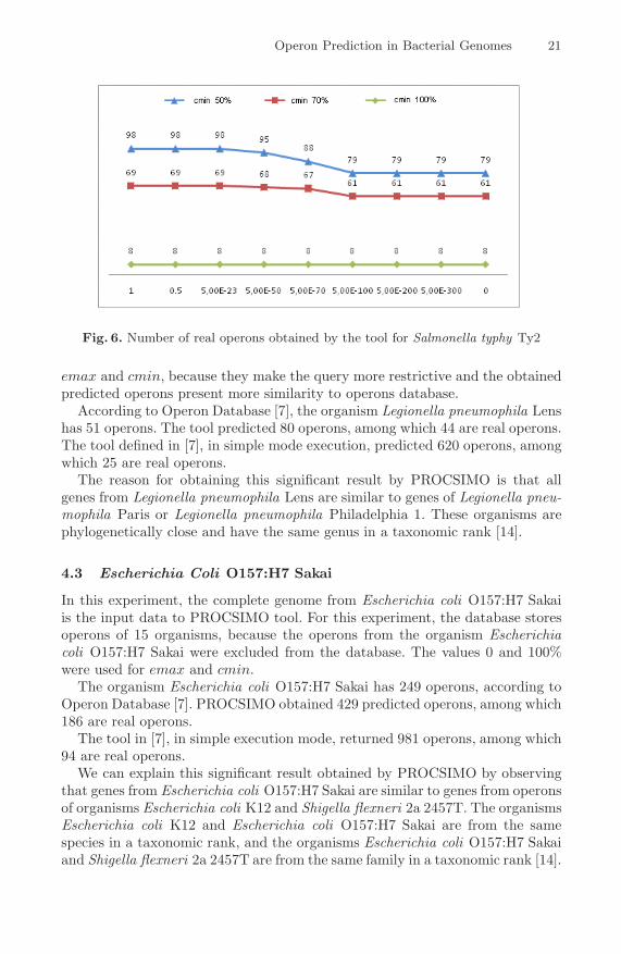
Fig. 6. Number of real operons obtained by the tool for Salmonella typhy Ty2
emax and cmin, because they make the query more restrictive and the obtainedpredicted operons present more similarity to operons database.
According to Operon Database [7], the organism Legionella pneumophila Lenshas 51 operons. The tool predicted 80 operons, among which 44 are real operons.The tool defined in [7], in simple mode execution, predicted 620 operons, amongwhich 25 are real operons.
The reason for obtaining this significant result by PROCSIMO is that allgenes from Legionella pneumophila Lens are similar to genes of Legionella pneu-mophila Paris or Legionella pneumophila Philadelphia 1. These organisms arephylogenetically close and have the same genus in a taxonomic rank [14].
4.3 Escherichia Coli O157:H7 Sakai
In this experiment, the complete genome from Escherichia coli O157:H7 Sakaiis the input data to PROCSIMO tool. For this experiment, the database storesoperons of 15 organisms, because the operons from the organism Escherichiacoli O157:H7 Sakai were excluded from the database. The values 0 and 100%were used for emax and cmin.
The organism Escherichia coli O157:H7 Sakai has 249 operons, according toOperon Database [7]. PROCSIMO obtained 429 predicted operons, among which186 are real operons.
The tool in [7], in simple execution mode, returned 981 operons, among which94 are real operons.
We can explain this significant result obtained by PROCSIMO by observingthat genes from Escherichia coli O157:H7 Sakai are similar to genes from operonsof organisms Escherichia coli K12 and Shigella flexneri 2a 2457T. The organismsEscherichia coli K12 and Escherichia coli O157:H7 Sakai are from the samespecies in a taxonomic rank, and the organisms Escherichia coli O157:H7 Sakaiand Shigella flexneri 2a 2457T are from the same family in a taxonomic rank [14].

22 M.B.S. Barros, S. de L. Martins, and A. Plastino
5 Conclusions
This paper presents an extension to the PROCSIMO tool [4] and its maincontribution is a new method for operon prediction in bacterial genomes.
The results obtained for operon prediction were quite significant and betterthan results obtained by another operon prediction tool proposed in [7]. Wegot better results when the input genomes were from organisms which werephylogenetically close to one or more organisms of the operons database.
At present, the PROCSIMO operons database is small, and we believe thatthis tool will be able to find more real operons as more organism operons arestored in the tool database.
The average execution time for operon prediction by this tool is 30 minutes,and we believe that we can decrease this time by optimizing the code. Since theprocedure of operon prediction requires many BLAST executions over a greatnumber of gene pairs, we think that a code parallelization could be performedin order to decrease the processing time.
References
1. Bergman, N.H., Passalacqua, K.D., Hanna, P., Qin, Z.S.: Operon prediction forsequenced bacterial genomes without experimental information. Applied and En-vironmental Microbiology 73, 846–854 (2007)
2. Ermolaeva, M.D., White, O., Salzberg, S.L.: Prediction of operons in microbialgenomes. Nucleic Acids Research 29, 1216–1221 (2001)
3. Hodgman, T.C.: A historical perspective on gene/protein functional assignment.Bioinformatics 16, 10–15 (2000)
4. Azevedo, C.V.: Procura de similaridade entre operons. Master’s thesis, Departa-mento de Ciencia da Computacao, Universidade Federal Fluminense, Niteroi (2003)
5. Craven, M., Page, D., Shavlik, J., Bockhorst, J., Glasner, J.: A probabilistic learn-ing approach to whole-genome operon prediction. In: Proceedings of the 8th In-ternational Conference on Intelligent Systems for Molecular Biology, pp. 116–127(2000)
6. Moreno-Hagelsieb, G., Collado-Vides, J.: A powerful non-homology method for theprediction of operons in prokaryotes. Bioinformatics 18, S329–S336 (2002)
7. Okuda, S., Katayama, T., Kawashima, S., Goto, S., Kanehisa, M.: Odb: a databaseof operons accumulating known operons across multiple genomes. Nucleic AcidsResearch 34, D358–D362 (2005)
8. Altschul, S.F., Gish, W., Miller, W., Myers, E.W., Lipman, D.J.: Basic local align-ment search tool. Journal of Molecular Biology 215, 403–410 (1990)
9. Korf, I., Yandell, M., Bedell, J.: BLAST: An Essential Guide to the Basic LocalAlignment Search Tool, 1st edn. O’Reilly & Associates, Sebastopol (2003)
10. Benson, D.A., Karsch-Mizrachi, I., Lipman, D.J., Ostell, J., Wheeler, D.L.: Gen-bank. Nucleic Acids Research 35, D21–D25 (2007)
11. Perl: The Perl Directory - perl. org. (2005), www.perl.org12. MySQL: Database server (2005), www.mysql.com13. Apache: Apache: Servidor WEB (2005), http://httpd.apache.org/14. NCBI: National Center for Biotechnology Information (2007),
http://www.ncbi.nlm.nih.gov/sites/entrez?db=taxonomy

An Evaluation of the Impact of Side Chain
Positioning on the Accuracy of Discrete Modelsof Protein Structures�
Miguel M.F. Bugalho and Arlindo L. Oliveira
INESC-ID/IST, R. Alves Redol 9, 1000 LISBOA, [email protected], [email protected]
Abstract. Discrete models are important to reduce the complexity ofthe protein folding problem. However, a compromise must be made be-tween the model complexity and the accuracy of the model.
Previous work by Park and Levitt has shown that the protein back-bone can be modeled with good accuracy by four state discrete models.Nonetheless, for ab-initio protein folding, the side chains are importantto determine if the structure is physically possible and well packed.
We extend the work of Park and Levitt by taking into account thepositioning of the side chain in the evaluation of the accuracy. We showthat the problem becomes much harder and more dependent on the typeof protein being modeled. In fact, the structure fitting method used intheir work is no longer adequate to this extended version of the problem.We propose a new method to test the model accuracy.
The presented results show that, for some proteins, the discrete mod-els with side chains cannot achieve the accuracy of the backbone onlydiscrete models. Nevertheless, for the majority of the proteins an RMSDof four angstrom or less is obtained, and, for many of those, we reach anaccuracy near the two angstrom limit. These results prove that discretemodels can be used in protein folding to obtain low resolution models.Since the side chains are already present in the models, the refinementof these solutions is simpler and more effective.
Keywords: Protein models, discrete state models, side chain position-ing, protein folding.
1 Introduction
The ab-initio protein folding problem consists in determining the structure of aprotein using only the information of its amino acid sequence. Even extremelysimplified versions of this problem have been proved to be NP-Hard [1,2,3,4].
In a protein structure there are several structural constrains. For the atomicangles and bond lengths the variation is small and, thus, the majority of thefolding algorithms focus on the dihedral angles. In addition to the structural� Partially supported by project Biogrid POSI/SRI/47778/2002 and by the Portuguese
Science and Technology Foundation by grant SFRH/BD/13215/2003.
A.L.C. Bazzan, M. Craven, and N.F. Martins (Eds.): BSB 2008, LNBI 5167, pp. 23–34, 2008.c© Springer-Verlag Berlin Heidelberg 2008

24 M.M.F. Bugalho and A.L. Oliveira
constrains, the protein structures are defined by the atomic interactions. Al-though the dihedral angles have optimal values they usually assume differentvalues to allow for interactions between atoms.
In the context of this work, a discrete state model is an all heavy atomsprotein model that uses a discrete set for the possible values of the dihedralangles. The atomic bond lengths and angles are considered fixed at the optimalvalues. Previous work [5] has shown that discrete state models with a limitednumber of states (four) can describe proteins with relatively good accuracy. Inthat work the authors have also shown that, for the same degree of complexity,off lattice discrete state models are more accurate than lattice models.
In the work of Park and Levitt only the main chain is used and no considera-tion is made for clashes between atoms. In this work we will analyze the accuracyof discrete state models using an all heavy atoms representation and disallowingatomic clashes. Using all heavy atoms representations requires positioning of theside chains. A simple positioning method based in rotamer libraries is proposed.
1.1 Motivation
Although important studies on the accuracy and application of discrete mod-els were published more then 10 years ago [5,6], discrete models are still beingstudied and applied to problems in recently published works. Discrete modelsare used in studies for ab-initio protein folding [7,8]. Recent works also use dis-crete models for generating ensembles of structures [9,10]. The study of discreteprotein models is, therefore, highly relevant. Although the models presented byPark and Levitt are used in protein folding problems, the models were onlyshown to be accurate for modeling the backbone. Using only backbone modelscan produce physically impossible models. Moreover, depending on the scoringfunction, these models may have a high score and may be chosen as the bestmodel. Therefore, to avoid physically impossible models, we have extended thiswork by considering side chain position and atomic clashes.
Discrete models are particulary fit to perform high level structure search, sincethe search space is greatly reduced and very similar structures can be more easilyavoided. The applicability of the discrete models relies on the solution of threedifficulties, since discrete models:
– Require a scoring function that can ignore the atomic details giving highscores to physically inexact, near native structures.
– Need a search technique that can efficiently search the structure space with-out enumerating all the structures, since the space size is still exponentialon the size of the protein.
– Need to use a set of dihedral angle values that can accurately model theprotein. An accurate model must have a low root mean square distance tothe native structure but must also have feasible physical properties like:secondary structure, atomic contacts and lack of atomic clashes. This isimportant since the scoring function must be able to find, in the models,characteristics that are similar to the characteristics of native protein.

An Evaluation of the Impact of Side Chain Positioning on the Accuracy 25
The first difficulty can be solved using a statistical scoring function. Thesecond is the final step towards finding a near native structure and a numberof techniques have been proposed. However, the search will only work if a gooddiscrete model is available. The third difficulty is, therefore, the focus of thiswork.
As referred before, the model must be able not only to approximate the atomicpositions of the native structure, but also to avoid unfeasible structures, e.g.structures with atomic clashes or unrealistic side chain conformations. Therefore,we will analyze the accuracy of known discrete models, while considering clashesand side chain positioning.
2 Side Chain Positioning
One of the most used methods for side chain positioning is based on the useof rotamers libraries. In this work we used the Dunbrack Backbone-DependentRotamer Library [11,12,13,14] which contains information about each amino acidside chain. For each amino acid, the library has the side chain dihedral anglevalues indexed by the backbone φ/ψ pairs in slots of 10 degrees. The library alsocontains the observed frequency of the side chain dihedral angles in the particularslot. To reduce the number of possible conformations we used the frequencyinformation contained in the library to prune less probable configurations. Unlessotherwise stated, a 0.04 (4%) frequency cutoff was used.
The decision to use a rotamer method was made for two reasons:
– The method creates a discretized set of highly probable configurations. Thisavoids the usage of continuous minimization methods.
– Since the rotamers are indexed by φ and ψ backbone angles, there is no needto verify clashes between atoms of the same amino acid.
In this paper we present a simple positioning algorithm that tests the pos-sible rotamer conformations until a valid conformation is found. The frequencyinformation is used to establish the testing order. Rotamers that occur morefrequently in known proteins will be tested first. Notice that we only want toverify if there is a possible side chain configuration and not to set the best one.The best side chain conformation can be set in the end during refinement using,for example, the SCWRL program [15], which sets the side chain using a graphtheory based algorithm and an energy function. Since SCWRL does not changethe backbone it is essential that sufficient space is left for the side chains.
After choosing a possible configuration, the algorithm continues to constructthe protein model by extending the backbone configuration. However, this par-ticular choice of the side chain configuration can be changed latter. The sidechain is modified if, afterwards, that particular side chain configuration preventsother side chains from being positioned. When a clash between side chains is de-tected (no changes in previous backbone atoms are allowed) the algorithm setsthe new side chain in the configuration with less conflicts and tries to reconfigurethe old side chain. If a new side chain conflict is found the process is restarted

26 M.M.F. Bugalho and A.L. Oliveira
Fig. 1. Example of a successful side chain reconfiguration. Both the backbone, strongerlines, and the side chains are represented. The red sphere shows the side chain conflictbetween the new side chain and a previously set side chain. A new configuration ischosen for the older side chain by rotating it to the opposite side of the new side chainposition.
until a predefined threshold for the number of side chain changes is reached.Figure 1 shows a example of successful side chain reconfiguration.
If an unresolvable conflict is found, like a side chain versus backbone conflict,or the backtrack threshold is reached, the algorithm considers that there is notenough space for the side chain and reports a clash. To avoid loops the algorithmdoes not allow for the same side chain to be changed twice.
3 Discrete State Model
Previous work [5] has tested various discrete state models and presented somereasonably accurate sets of states. The test made by Park and Levitt consistedin fitting the discrete models into the backbone of the known structure. The sidechains, and possible clashes between atoms, were not considered in the fittingproblem. In this section we will analyze some of the models described by Parkand Levitt in a test platform that considers side chains and atomic clashes.
Table 1 shows the discrete models previously proposed [5]. We used four ofthese discrete models: three four states models and one six states model. Wehave chosen the Rooman et al. six states model since it obtained better resultsthan the one proposed by Park and Levitt. In the four states models, we chosemodel C because it was the best model, and model A because it obtained thebest results for the Alpha and Beta secondary structures. Model G was chosenrandomly from the rest.
Table 1. Discrete State models used in the work of Park and Levitt [5]. The ∗ signalsthe models used in this work.
Name Set of Pairs of Angles Name Set of Pairs of Angles
∗ A (-64,-40),(-123,134),(111,-46),(117,105) B (-66,-40),(-119,114),(-36,124),(132,-40)
∗ C (-63,-63),(-132,115),(-42,-41),(-44,127) D (-58,-31),(-127,126),(-97,-24),(109,108)
E (-71,-57),(-131,122),(-42,-36),( 107,-25) F (-58,-51),(-133,135),(-33,174),(114,-40)
∗ G (-56,-48),(-129,128),(-108,35),(-31,-109) H (-74,-31),(-131,125),(-101,179),(105,-40)
6 states (-57,-47),(-139,135),(-119,113), ∗ Rooman (-65,-42),(-123,139),(-70,138),(-49,-26),(-106,48),(-101,-127) et al.[6] (-87,-47),(77,22),(107,-174)
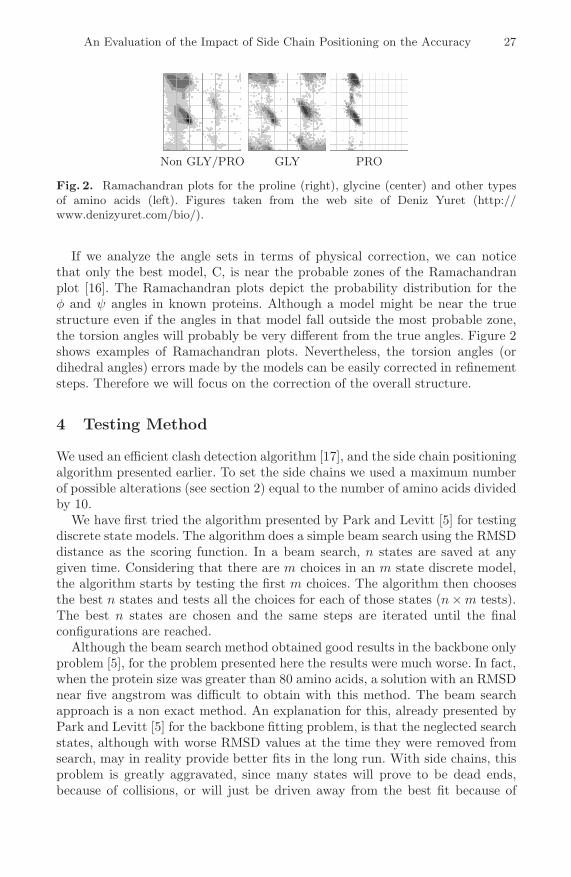
An Evaluation of the Impact of Side Chain Positioning on the Accuracy 27
Non GLY/PRO GLY PRO
Fig. 2. Ramachandran plots for the proline (right), glycine (center) and other typesof amino acids (left). Figures taken from the web site of Deniz Yuret (http://www.denizyuret.com/bio/).
If we analyze the angle sets in terms of physical correction, we can noticethat only the best model, C, is near the probable zones of the Ramachandranplot [16]. The Ramachandran plots depict the probability distribution for theφ and ψ angles in known proteins. Although a model might be near the truestructure even if the angles in that model fall outside the most probable zone,the torsion angles will probably be very different from the true angles. Figure 2shows examples of Ramachandran plots. Nevertheless, the torsion angles (ordihedral angles) errors made by the models can be easily corrected in refinementsteps. Therefore we will focus on the correction of the overall structure.
4 Testing Method
We used an efficient clash detection algorithm [17], and the side chain positioningalgorithm presented earlier. To set the side chains we used a maximum numberof possible alterations (see section 2) equal to the number of amino acids dividedby 10.
We have first tried the algorithm presented by Park and Levitt [5] for testingdiscrete state models. The algorithm does a simple beam search using the RMSDdistance as the scoring function. In a beam search, n states are saved at anygiven time. Considering that there are m choices in an m state discrete model,the algorithm starts by testing the first m choices. The algorithm then choosesthe best n states and tests all the choices for each of those states (n×m tests).The best n states are chosen and the same steps are iterated until the finalconfigurations are reached.
Although the beam search method obtained good results in the backbone onlyproblem [5], for the problem presented here the results were much worse. In fact,when the protein size was greater than 80 amino acids, a solution with an RMSDnear five angstrom was difficult to obtain with this method. The beam searchapproach is a non exact method. An explanation for this, already presented byPark and Levitt [5] for the backbone fitting problem, is that the neglected searchstates, although with worse RMSD values at the time they were removed fromsearch, may in reality provide better fits in the long run. With side chains, thisproblem is greatly aggravated, since many states will prove to be dead ends,because of collisions, or will just be driven away from the best fit because of

28 M.M.F. Bugalho and A.L. Oliveira
them. Because of these results we present a new search method that, althoughcomputationally more expensive (exponential number of tests instead of n×mtests), can avoid this problem. The algorithm performs a backtrack search havingtherefor exponential complexity. However, as we are going to show in the resultssection, in the majority of the cases a solution is found in reasonable time.
Algorithm 1. Testing method for the discrete models1: procedure FitModel(Pdb,Model)2: RmsdLimit = 53: Start with the first amino acid of the sequence4: while RmsdLimit > 1 and there is a possible (φ, ψ) pair do5: Choose argmin(φ,ψ) RMSD ({non tested (φ, ψ) pairs of Model})6: if RMSD<RmsdLimit and no backbone clash with previous atoms then7: for all rotamers indexed by (φ, ψ) do8: if the side chain does not clash with any previous atom then9: Set the Next Amino Acid
10: if no side chain was found then11: Choose rotamer with less conflicts and change previous side chains12: if no correction is possible then13: Execute a Backtrack14: else15: Set the Next Amino Acid16: else17: Execute a Backtrack
procedure Backtrack � The chosen (φ,ψ) pair is not a possible configurationif ∃ non tested (φ, ψ) pairs of Model then
Test the next (φ, ψ) pair with lowest RMSD (step 5)else
Backtrack to previous amino acid,test next lowest RMSD (φ, ψ) pair (step 4)
procedure Next Amino Acid � A valid conformation was foundif this is the last amino acid of the sequence then
RmsdLimit = RmsdLimit - 0.2Re-evaluate this amino acid with the new limit (step 5)
elseSet the next amino acid (step 4)
Each discrete state model is tested by searching in the discrete state searchspace. Algorithm 1 presents the testing method proposed in this work. Thesearch is performed by fitting the model to the real protein, using a best firstapproach with backtrack. For each amino acid, if the backbone conformationwith lowest RMSD has no conflict with the previously set atoms, and if a nonconflicting rotamer configuration is found, the algorithm sets the atoms andtries to set the next amino acid (running the Next Amino Acid procedure).During this step, previous side chains may be repositioned to accommodate thenew amino acid atoms. If a clash is found that cannot be resolved or if the

An Evaluation of the Impact of Side Chain Positioning on the Accuracy 29
root mean square distance between the model and the protein exceeds a giventhreshold, the algorithm backtracks (running the Backtrack procedure). Whilebacktracking, one of two actions occurs: if some of the possible configurationsfor the backbone were not tested the algorithm chooses the next conformationwith lowest RMSD; if all configurations were tested the algorithm returns to thepreviously set amino acid and resumes its main procedure.
The algorithm starts with a minimum RMSD threshold of 5 angstrom anddecrements 0.2 angstrom each time a model is found for the previous threshold.The algorithm stops if one of the following conditions is met: a 1 angstromRMSD threshold limit is reached, no more configurations are possible or a timelimit of one hour for each one hundred amino acids is reached. We considereddifferent thresholds for the side chain rotamer library (see section 2). In additionto the 4% default value, we also tried 1%, 0.1% and without any cutoff (completerotamer library). Since there is a time limit, considering more rotamers or a morecomplex model may or may not produce better results.
5 Results
To test the accuracy of discrete models we compiled a set of protein structuresof increasing size. The proteins also differ in terms of secondary structure com-position (Alpha Beta, Mainly Alpha and Mainly Beta proteins). Table 2 showsthe set of chosen proteins and figure 3 shows the respective structures.
We have chosen different types of proteins and different sizes to study theimpact of these features in the precision of the discrete models. We decided tofocus our choice in globular proteins which are more packed and therefore moredifficult.
Figure 4 shows the results using side chains cutoff of 4% and 1%. Figure 5shows the results when using 0.1% and the complete rotamer library.
From the results in figure 4 it is possible to verify that, for the majority of theproteins an accurate model can be found. However, for some proteins, it is hard tofind a model and, in some cases, no model can be found. For the smaller proteins(less that 100 amino acids), in the cases where an accurate model was found, the
Table 2. Protein data set
Name Size Type Name Size Type
1r69 63 Mainly Alpha 1co6 107 Mainly Alpha1aho 65 Alpha Beta 1a1x 107 Manly Beta (beta barrel)1ctf 69 Alpha Beta 1mai 120 Alpha Beta1hyp 75 Manly Alpha 1vhh 157 Alpha Beta1poh 85 Alpha Beta 1b56 134 Manly Beta (beta barrel)1opd 86 Alpha Beta 1kao 167 Alpha Beta1o5u 88 All Beta (beta helix) 1pt6 192 Alpha Beta1tig 89 Alpha Beta 1vec 206 Alpha Beta
1bm8 100 Alpha Beta 1tjy 316 Alpha Beta1e9m 106 Alpha Beta 1pot 322 Alpha Beta

30 M.M.F. Bugalho and A.L. Oliveira
1r69 1aho 1ctf 1hyp 1poh 1opd 1o5u
1tig 1bm8 1e9m 1co6 1a1x 1mai 1vhh
1b56 1kao 1pt6 1vec 1tjy 1pot
Fig. 3. Protein data set
results are consistent with the ones obtained for the backbone fitting problem[5] (2.22 to 2.43 angstrom for the four states models and 1.74 for the six statesmodel). The problem is much easier in this case since the error accumulationin the fitting will be small, and also because many of the side chains can bepositioned by choosing a conformation that points to the exterior of the protein.
The side chain will only affect the fit in places where the protein is morecompact. In those places, the minor errors in the discrete state models may notprovide enough space for the side chains to be positioned. It is possible thata better fit exists even for the larger proteins, however, the fitting problem isNP Hard and the size of the problem does not allow for a complete search.Nevertheless, a less than 5 angstrom fit was found even for the larger proteins.
The cases where the results are worse in the side chain discrete models happenmainly with proteins with a large number of beta structures (1o5u) or that havea dense core (1vhh). In the first case, because the flexibility of the beta structuresis harder to model and in the second case, because it is harder to pack the atoms.
We also verify that, for the four states models, the best results are obtainedby the A model for the 4% and by the C model for the 1% cutoff. For theresults on the 1% cutoff the A model performs better in the proteins with morebeta structures. This is expected since the A model dihedral angles representbetter the beta structures and the C model the alpha structures. However, thebeta structures are flexible and even the A model cannot fully represent them.Therefor the C model will normally perform better then the A model, unless thefitting error in beta structures is too great to be recovered from, or the numberof beta structures is high. That is probably the case with the 4% cutoff. In this

An Evaluation of the Impact of Side Chain Positioning on the Accuracy 31
Fig. 4. Results of the Discrete State Models Using Side Chain cutoff of 4% and 1%
case, the errors are greater and the search algorithm for the C model cannot afind a reasonable fit for the beta structures (for instance: two strands must beplaced further apart because the side chains colide).
The six states model performs better than the four states models. However,the increase in the performance would probably not compensate for the increasein search space in a search procedure. Notice that, in this problem we are usingthe root mean square distance (RMSD) instead of the scoring functions used inab-initio folding. The information given by a scoring function is less precise andthe space that needs to be searched is much greater, even in a four state model.In a six state model that space will be even greater. We can probably achieve thesame result from a four states model after a refinement process and we wouldbenefit greatly from the smaller size of the search space during the search pro-cess. From figures 4 and 5 we can see the impact of the size of the rotamerlibrary in the search. The performance of the models usually increases with thesize of the rotamer library. However it is possible to verify that, for the biggeror more compact proteins, the performance sometimes decreases. For instance,for the 0.1% cutoff, the C model in 1poh and all models in 1e9m perform worse

32 M.M.F. Bugalho and A.L. Oliveira
Fig. 5. Results of the Discrete State Models Using Side Chain cutoff of 0.1 percent andusing all side chains in the rotamer library
than in the 4% cutoff. When we avoid the cutoff we can see this result again (6state model for the 1e9m protein). This happens because, when we increase thesize of the library, a greater number of side chain conformations may be tested.Consequently, although some conflicts may now be avoidable, the cost of theextra tests might not allow for the same number of conformations to be tested.This increase of time for each side chain positioning will have an even greaterimpact in an ab-initio search algorithm, since no exact measure like the RMSDexists. Without an exact measure, the number of wrong conformations searchedwill be much greater and the increased computational cost of the enlarged librarywill further decrease the performance.
The type of model used and the threshold limit will have to be chosen accord-ing to the type of proteins (specially their secondary structure and size) and thesearch algorithm. For a search algorithm, with no specific information, a fourstates model, specially a generic one like the C model, with a side chain threshold

An Evaluation of the Impact of Side Chain Positioning on the Accuracy 33
of 1% will probably have best results because of the increase in the size of thesearched space. If the protein is small, there are fewer possible conformations,and more detailed models can be found using more rotamers or even using thesix states model. For specific cases, where there is some information about theprotein, a model that increases the performance can probably be built.
Notice that if we use a threshold limit of, for instance, five angstrom, and wecannot find a model, we cannot be sure that no model can reach a 5 angstromRMSD. When we stop the model construction, it is above the threshold, butsubsequent choices could lower the RMSD. We chose not to pursue an exactsolution since we needed to explore an search space that would be exponentialto the size of the protein i.e. the time needed for the search would be to higheven for the smaller proteins.
6 Discussion
The results show that, although the discrete models presented previously [5] arewell optimized for backbone fitting, when side chains are used and clashes aredisallowed the accuracy decreases greatly for some proteins.
For small proteins the problem does not exist, since the side chains maybe set to the outside of the structure. However, for larger proteins, especiallyfor proteins with beta sheets, the accuracy is significantly lower than the oneobtained for the backbone only tests. However, it is possible to obtain structureswith root mean square error close or lower than 4 angstrom, which is still avery good, low detail, representation for the protein and a good starting pointfor the refinement algorithms. Moreover, for many proteins the results are nearthe 2 angstrom RMSD value and have, therefore, an accuracy equivalent to thebackbone discrete models. The results also show that above a determined proteinsize the RMSD of the obtained models depends more on the type of the proteinthan on the size increase i.e. even for the bigger proteins good models can beobtained.
Since even low detail structures are very useful to determine protein function,these results show that the presented discrete models may be used in ab-initioprotein folding. Furthermore, in the protein folding process, one important as-pect is that the scoring function is well adapted to the model that is being used.The model must be able to represent the positive and negative aspects of thestructure, in a way that the scoring function can detect. With this work we notonly prove that we can obtain a near the native protein structure, but also, byconsidering side chains and disallowing clashes, we have already obtained phys-ically correct structures. This reduces the noise for the scoring function, sincepositive aspects of a structure, like the proximity of two amino acids, could bepresent in a physically impossible structure.
In future work we propose to study efficient algorithms to search near nativeconformations in the discrete state model space.
34 M.M.F. Bugalho and A.L. Oliveira
References
1. Fraenkel, A.S.: Complexity of protein folding. Bulletin of Mathematical Biol-ogy 55(6), 1199–1210 (1993)
2. Crescenzi, P., Goldman, D., Papadimitriou, C.H., Piccolboni, A., Yannakakis, M.:On the complexity of protein folding. Journal of Computational Biology 5(3), 423–466 (1998)
3. Berger, B., Leighton, T.: Protein folding in the hydrophobic-hydrophilic (HP) isNP-complete. In: Proceedings of the Second Annual International Conference onComputational Molecular Biology, pp. 30–39 (1998)
4. Hart, W.E., Istrail, S.: Robust proofs of NP-hardness for protein folding: generallattices and energy potentials. Journal of Computational Biology 4(1), 1–22 (1997)
5. Park, B.H., Levitt, M.: The complexity and accuracy of discrete state models ofprotein structure. Journal of Molecular Biology 249, 493–507 (1995)
6. Rooman, M.J., Kocher, J.P., Wodak, S.J.: Prediction of protein backbone con-formation based on seven structure assignments. Influence of local interactions.Journal of Molecular Biology 221(3), 961–979 (1991)
7. Gibbs, N., Clarke, A.R., Sessions, R.B.: Ab initio protein structure prediction usingphysicochemical potentials and a simplified off-lattice model. Proteins StructureFunction and Genetics 43(2), 186–202 (2001)
8. Huang, E.S., Koehl, P., Levitt, M., Pappu, R.V., Ponder, J.W.: Accuracy of side-chain prediction upon near-native protein backbones generated by ab initio foldingmethods. Proteins Structure Function and Genetics 33(2), 204–217 (1998)
9. Ma, B., Nussinov, R.: The Stability of Monomeric Intermediates Controls AmyloidFormation: A β 25-35 and its N27Q Mutant. Biophysical Journal 90(10), 3365–3374(2006)
10. DePristo, M.A., de Bakker, P.I.W., Lovell, S.C., Blundell, T.L.: Ab initio con-struction of polypeptide fragments: Efficient generation of accurate, representativeensembles. Proteins Structure Function and Genetics 51(1), 41–55 (2003)
11. Dunbrack, R.L., Karplus, M.: Conformational analysis of the backbone-dependentrotamer preferences of protein sidechains. Nature Structural Biology 1(5), 334–340(1994)
12. Dunbrack Jr., R.L.: Rotamer libraries in the 21st century. Current Opinion inStructural Biology 12(4), 431–440 (2002)
13. Dunbrack Jr., R.L., Cohen, F.E.: Bayesian statistical analysis of protein side-chainrotamer preferences. Protein Science 6(8), 1661–1681 (1997)
14. Dunbrack Jr., R.L., Karplus, M.: Backbone-dependent rotamer library for proteins.Application to side-chain prediction. Journal of Molecular Biology 230(2), 543–574(1993)
15. Canutescu, A.A., Shelenkov, A.A., Dunbrack, R.L.: A graph-theory algorithm forrapid protein side-chain prediction. Protein Science 12(9), 2001–2014 (2003)
16. Ramakrishnan, C., Ramachandran, G.N.: Stereochemical criteria for polypeptideand protein chain conformations: II. Allowed conformations for a pair of peptideunits. Biophysical Journal 5(6), 909 (1965)
17. Bugalho, M., Oliveira, A.L.: An efficient clash detection method for molecularstructures. Technical Report 21, INESC-ID (August 2007)

Top-Down Hierarchical Ensembles of Classifiers
for Predicting G-Protein-Coupled-ReceptorFunctions
Eduardo P. Costa1, Ana C. Lorena2, Andre C.P.L.F. Carvalho1,and Alex A. Freitas3
1 Depto. Ciencias de ComputacaoICMC/USP - Sao Carlos - Caixa Postal 668
13560-970 - Sao Carlos-SP, Brazil{ecosta,andre}@icmc.usp.br
2 Universidade Federal do ABC09.210-170 - Santo Andre-SP, Brazil
[email protected] Computing Laboratory and Centre for BioMedical Informatics
University of Kent, Canterbury, CT2 7NF, [email protected]
Abstract. Despite the recent advances in Molecular Biology, the func-tion of a large amount of proteins is still unknown. An approach that canbe used in the prediction of a protein function consists of searching againstsecondary databases, also known as signature databases. Different strate-gies can be applied to use protein signatures in the prediction of functionof proteins. A sophisticated approach consists of inducing a classificationmodel for this prediction. This paper applies five hierarchical classifica-tion methods based on the standard Top-Down approach and one hierar-chical classification method based on a new approach named Top-DownEnsembles - based on the hierarchical combination of classifiers - to threedifferent protein functional classification datasets that employ protein sig-natures. The algorithm based on the Top-Down Ensembles approach pre-sented slightly better results than the other algorithms, indicating thatcombinations of classifiers can improve the performance of hierarchicalclassification models.
1 Introduction
Proteins are large organic compounds that perform almost all the functionsrelated to cell activity, such as biochemical reactions, cell signaling, structuraland mechanical functions. These large molecules consist of long sequences ofamino acids, which fold into specific structures so that the protein can functionproperly.
In functional genomic, an important problem is the prediction of the functionof proteins. Due to the recent advances in Molecular Biology methods and the
A.L.C. Bazzan, M. Craven, and N.F. Martins (Eds.): BSB 2008, LNBI 5167, pp. 35–46, 2008.c© Springer-Verlag Berlin Heidelberg 2008

36 E.P. Costa et al.
consequent generation of biological data in large scale, data analysis has becomea central issue for the investigation of proteins whose functions are unknown.
An approach that can be used in the prediction of a protein function involvessearching against secondary databases, also known as signature databases. Thesedatabases contain results of analysis performed in primary databases, which con-tain linear sequences of amino acids, and can be used to verify the presence ofparticular patterns in the query proteins. These patterns represent informationabout conserved motifs in proteins, which are frequently useful to help the pre-diction of protein functions. Protein signatures can be used to assign a queryprotein to a specific family of proteins and thus to formulate hypotheses aboutits function [1]. Examples of signature databases include InterPro [2], Prosite[3], Pfam [4] and Prints [5].
Different strategies can be applied to use protein signatures in the prediction offunction of proteins. A sophisticated approach consists of inducing a classificationmodel for this prediction. Accordingly, each protein is represented by an attributeset, describing the presence or absence of patterns in the protein, and a learningalgorithm captures the most important relationships between the attributes andthe classes involved in the classification problem.
In the context of prediction of protein function, a classification model needsto be induced according to a special kind of classification problem named hierar-chical classification, since protein functional data is inherently hierarchical (forexample, the Enzyme Commission hierarchy [6]).
In this paper, three protein function datasets are analyzed - each one em-ploying one different kind of protein signature - for a comparative study amongsix hierarchical classification algorithms. The algorithm based on the Top-DownEnsembles approach - a variation of the Top-Down approach that uses combina-tion of classifiers for the induction of the classification model - presented betterresults across the three different kinds of protein signatures - Prosite, Pfam andPrints. The main contribution of this paper is to show that combinations ofclassifiers can improve the performance of hierarchical classification models, aresult that was consistent even for different types of protein signatures.
The paper is organized as follows: Section 2 introduces important conceptsof hierarchical classification; Section 3 introduces the Top-Down Ensembles ap-proach; Section 4 discusses the materials and methods employed in the experi-ments performed in this work; Section 5 presents the experimental results; andSection 6 has the main conclusions from this work.
2 Hierarchical Classification
Classification is one of the most important problems in Machine Learning (ML)and Data Mining (DM) [7]. Given a dataset composed of n pairs (xi, yi), whereeach xi is a data item (example) and yi represents its class, a classificationalgorithm must find a function, through a training or adjustment phase, whichmaps each data item to its correct class.

Top-Down Hierarchical Ensembles of Classifiers 37
Fig. 1. Examples of hierarchies of classes: (a) Tree and (b) DAG
Conventional classification problems involve a finite (and usually small) setof flat classes. Each example is assigned to a class out of this set, in which theclasses do not have direct relationships to each other, such as subclass and super-class relationships. For this reason, these classification problems are named flatclassification problems. Nevertheless, there are more complex classification prob-lems where the classes to be predicted are hierarchically related [8,9,10]. Theseproblems are known in the ML literature as hierarchical classification problems.
The classes involved in a hierarchical classification problem can be disposedeither as a tree or as a Directed Acyclic Graph (DAG). The main differencebetween these structures is that, in the tree structure (Figure 1.a), each nodehas just one parent node, while in the DAG structure (Figure 1.b), each nodemay have more than one parent. The nodes represent the classes involved in theclassification problem and the root node corresponds to “any class”, denoting atotal absence of knowledge about the class of an object.
The deeper the class in the hierarchy, the more specific and useful is its associ-ated knowledge in the classification of a new data item. Hierarchical classificationproblems often have as objective to assigning a data item into one of the leafnodes. It may be the case, however, that the classifier does not have the desiredreliability to classify a data item into deeper classes. In this case, it would be saferto perform a classification into higher levels of the hierarchy. When all examplesmust be associated to classes in leaf nodes, the classification problem is named“mandatory leaf node prediction problem”. When this obligation does not hold,the classification problem is an “optional leaf node prediction problem”.
A simple approach to deal with a hierarchical classification problem consistsof reducing it into one or more flat classification problems. This reduction ispossible because a flat classification problem may be viewed as a particular caseof hierarchical classification, in which there are no subclasses and superclasses.However, the main disadvantage of this approach is to ignore the hierarchicalrelationships among the classes, which can provide valuable information for theinduction of a classification model. Two more sophisticated approaches thatconsider these relationships are the Top-Down and Big-Bang approaches [8].
The Top-Down approach uses the “divide and conquer” principle to inducethe classification model. The main idea of this approach is to produce one or
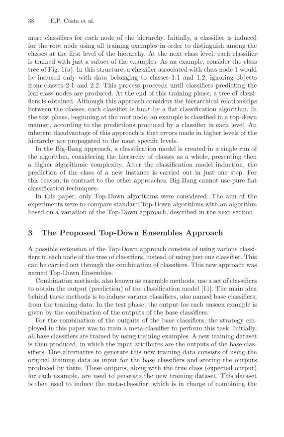
38 E.P. Costa et al.
more classifiers for each node of the hierarchy. Initially, a classifier is inducedfor the root node using all training examples in order to distinguish among theclasses at the first level of the hierarchy. At the next class level, each classifieris trained with just a subset of the examples. As an example, consider the classtree of Fig. 1(a). In this structure, a classifier associated with class node 1 wouldbe induced only with data belonging to classes 1.1 and 1.2, ignoring objectsfrom classes 2.1 and 2.2. This process proceeds until classifiers predicting theleaf class nodes are produced. At the end of this training phase, a tree of classi-fiers is obtained. Although this approach considers the hierarchical relationshipsbetween the classes, each classifier is built by a flat classification algorithm. Inthe test phase, beginning at the root node, an example is classified in a top-downmanner, according to the predictions produced by a classifier in each level. Aninherent disadvantage of this approach is that errors made in higher levels of thehierarchy are propagated to the most specific levels.
In the Big-Bang approach, a classification model is created in a single run ofthe algorithm, considering the hierarchy of classes as a whole, presenting thena higher algorithmic complexity. After the classification model induction, theprediction of the class of a new instance is carried out in just one step. Forthis reason, in contrast to the other approaches, Big-Bang cannot use pure flatclassification techniques.
In this paper, only Top-Down algorithms were considered. The aim of theexperiments were to compare standard Top-Down algorithms with an algorithmbased on a variation of the Top-Down approach, described in the next section.
3 The Proposed Top-Down Ensembles Approach
A possible extension of the Top-Down approach consists of using various classi-fiers in each node of the tree of classifiers, instead of using just one classifier. Thiscan be carried out through the combination of classifiers. This new approach wasnamed Top-Down Ensembles.
Combination methods, also known as ensemble methods, use a set of classifiersto obtain the output (prediction) of the classification model [11]. The main ideabehind these methods is to induce various classifiers, also named base classifiers,from the training data. In the test phase, the output for each unseen example isgiven by the combination of the outputs of the base classifiers.
For the combination of the outputs of the base classifiers, the strategy em-ployed in this paper was to train a meta-classifier to perform this task. Initially,all base classifiers are trained by using training examples. A new training datasetis then produced, in which the input attributes are the outputs of the base clas-sifiers. One alternative to generate this new training data consists of using theoriginal training data as input for the base classifiers and storing the outputsproduced by them. These outputs, along with the true class (expected output)for each example, are used to generate the new training dataset. This datasetis then used to induce the meta-classifier, which is in charge of combining the
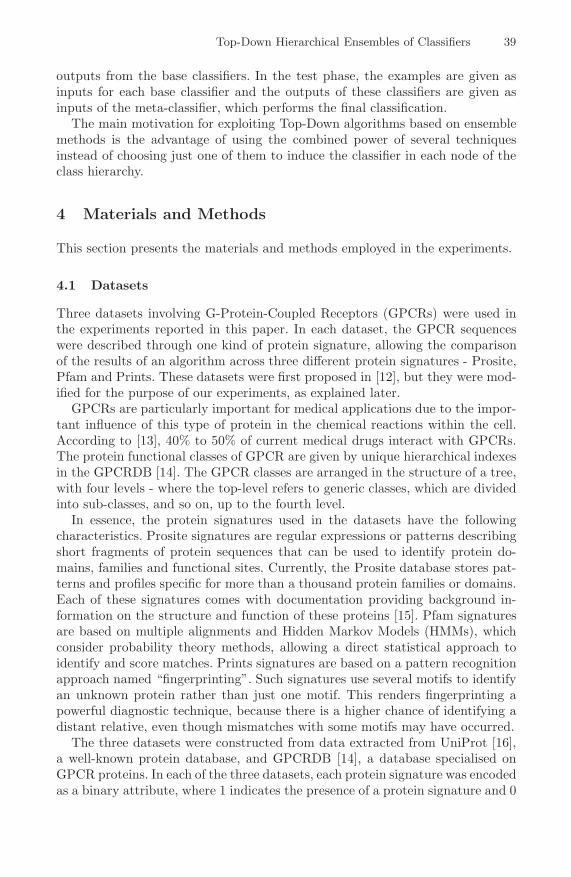
Top-Down Hierarchical Ensembles of Classifiers 39
outputs from the base classifiers. In the test phase, the examples are given asinputs for each base classifier and the outputs of these classifiers are given asinputs of the meta-classifier, which performs the final classification.
The main motivation for exploiting Top-Down algorithms based on ensemblemethods is the advantage of using the combined power of several techniquesinstead of choosing just one of them to induce the classifier in each node of theclass hierarchy.
4 Materials and Methods
This section presents the materials and methods employed in the experiments.
4.1 Datasets
Three datasets involving G-Protein-Coupled Receptors (GPCRs) were used inthe experiments reported in this paper. In each dataset, the GPCR sequenceswere described through one kind of protein signature, allowing the comparisonof the results of an algorithm across three different protein signatures - Prosite,Pfam and Prints. These datasets were first proposed in [12], but they were mod-ified for the purpose of our experiments, as explained later.
GPCRs are particularly important for medical applications due to the impor-tant influence of this type of protein in the chemical reactions within the cell.According to [13], 40% to 50% of current medical drugs interact with GPCRs.The protein functional classes of GPCR are given by unique hierarchical indexesin the GPCRDB [14]. The GPCR classes are arranged in the structure of a tree,with four levels - where the top-level refers to generic classes, which are dividedinto sub-classes, and so on, up to the fourth level.
In essence, the protein signatures used in the datasets have the followingcharacteristics. Prosite signatures are regular expressions or patterns describingshort fragments of protein sequences that can be used to identify protein do-mains, families and functional sites. Currently, the Prosite database stores pat-terns and profiles specific for more than a thousand protein families or domains.Each of these signatures comes with documentation providing background in-formation on the structure and function of these proteins [15]. Pfam signaturesare based on multiple alignments and Hidden Markov Models (HMMs), whichconsider probability theory methods, allowing a direct statistical approach toidentify and score matches. Prints signatures are based on a pattern recognitionapproach named “fingerprinting”. Such signatures use several motifs to identifyan unknown protein rather than just one motif. This renders fingerprinting apowerful diagnostic technique, because there is a higher chance of identifying adistant relative, even though mismatches with some motifs may have occurred.
The three datasets were constructed from data extracted from UniProt [16],a well-known protein database, and GPCRDB [14], a database specialised onGPCR proteins. In each of the three datasets, each protein signature was encodedas a binary attribute, where 1 indicates the presence of a protein signature and 0

40 E.P. Costa et al.
Table 1. Total number of examples, number of predictor attributes and number ofclasses per level (number of classes at level 1/2/3/4, respectively) of the three datasetsused in the experiments
Examples Attributes Classes per level
Prosite 5728 127 9/50/79/49
Pfam 6524 73 12/52/79/49
Prints 4880 281 8/46/76/49
its absence. Additionally, all datasets contain the attributes “molecular weight”and “sequence length”.
Besides the preprocessing steps explained in [12], another preprocessing stepwas included because a small subset of data belonged only to internal nodes ofthe hierarchy. As the developed algorithms consider mandatory leaf node predic-tion, some problems could take place during the evaluation of the classificationmodel. Suppose that an example belonging to an internal node was classifiedinto a class represented by a leaf node. During the evaluation, it would not bepossible to answer whether the prediction to the more specific node was success-ful or not. Therefore, examples belonging to internal nodes were not used in theexperiments.
In Table 1, the configuration obtained after preprocessing of the three datasets,regarding the total number of examples, number of predictor attributes and num-ber of classes per level (number of classes at level 1/2/3/4, respectively), areshown. As can be noticed in the table, the fourth level of the class hierarchies con-tain less classes than the third levels. It occurs because of the presence of severalleaf nodes in the third level of these hierarchies. Some leaf-nodes are also presentin the first and second levels.
All datasets were divided according to the 5-fold cross-validation methodology.Accordingly, each dataset is divided into five parts of approximately equal size.At each round, one fold is left for test and the remaining folds are used inthe classifiers training. This makes a total of five train and test sets. The finalaccuracy rate of a classification model is given by the mean of the predictiveaccuracies on the test sets from cross-validation.
4.2 Top-Down Hierarchical Classification Techniques
For developing the algorithm based on the hierarchical combination of classifiers,five different ML techniques selected, following distinct learning paradigms: De-cision Trees [17], induced with the C4.5 algorithm [18]; Sets of Rules induced bythe RIPPER algorithm [19]; Support Vector Machines (SVMs) [20]; K-nearestneighbors (KNN) [21]; and Bayesian Networks (BayesNet) [22]. In order to com-bine the outputs of the base classifiers, another classifier was used. For each nodeof the class hierarchies, the technique that induces the meta-classifier is chosenamong the ML techniques used to produce the base classifiers - the five MLtechniques previously mentioned. The adopted criterion consists of selecting the

Top-Down Hierarchical Ensembles of Classifiers 41
technique whose classifier presents the highest accuracy for the original trainingset.
In order to compare the results from the algorithm based on the Top-DownEnsembles approach with the other algorithms, the experiments also includedfive standard Top-Down hierarchical algorithms: one algorithm for each one ofthe five ML techniques employed in the hierarchical combination of classifiers.
All the Top-Down algorithms were implemented using packages from the Rtool [23]. The following packages were used: e1071 [24] and RWeka [25]. Thepackage e1071 was used to generate classifiers based on SVMs. The packageRWeka was used to generate classifiers for the other ML techniques. The defaultparameters were adopted for all techniques, except for SVM. For this technique,two parameters were modified: the cost was set to 100 and γ in the GaussianKernel was set to 0.01. These values were adopted because they are often used inprevious works involving SVMs, presenting good results. Besides, the continuousattributes were normalized before their use by SVMs. For the other techniques,the normalization was not necessary, either because this procedure does not affecttheir results or because the technique internally implements this procedure.
4.3 Evaluation of the Classification Models
The evaluation of the classification models was carried out level by level inthe classification hierarchy. For each hierarchical level, a value resulting fromthe evaluation of the predictive performance in the level is reported through ameasure called depth-dependent accuracy. This measure is based on an approachof attributing misclassification costs proposed in [26].
This approach takes into account that classes closer in the hierarchy tend tobe more similar to each other than classes more distant, and that predictionsin deeper levels are more difficult. Thus, misclassification costs for classes moredistant are higher than misclassification costs for classes closer to each other,and misclassification costs in the shallower levels are higher than in the deeperlevels. Accordingly, weights are attributed to the edges of the class tree and themisclassification costs are defined as the shortest weighted path between the trueclass and the predict class.
In the calculation of the depth-dependent accuracy, the misclassification costof each prediction is initially estimated through the division of the shortestweighted path between the true class and the predicted class by the value ofthe farthest weighted path from the node that represents the true class (i.e,the more distant class). After calculating the normalized distance for each mis-classification (for each test example), an average of all normalized distances isobtained. This average is the error rate of the classification model. Once theerror rate is obtained, the accuracy is defined by the complement of this value.The final accuracy rate of the classification model is then given by the mean ofthe predictive depth-dependent accuracies on the test sets generated by using5-fold cross-validation.
The weights used in the edges of the hierarchy for calculating the depth-dependent accuracy were: (0.26,0.13,0.07,0.04), where 0.26 is the weight of an
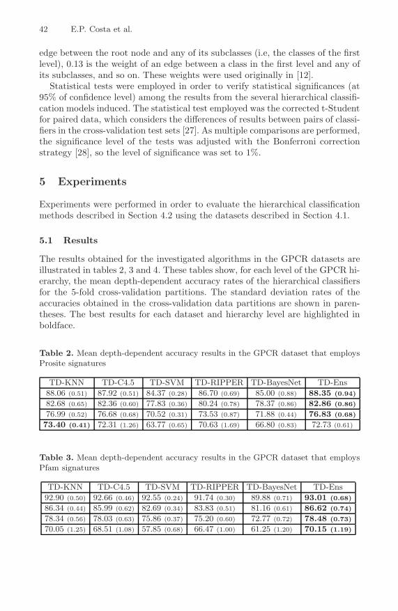
42 E.P. Costa et al.
edge between the root node and any of its subclasses (i.e, the classes of the firstlevel), 0.13 is the weight of an edge between a class in the first level and any ofits subclasses, and so on. These weights were used originally in [12].
Statistical tests were employed in order to verify statistical significances (at95% of confidence level) among the results from the several hierarchical classifi-cation models induced. The statistical test employed was the corrected t-Studentfor paired data, which considers the differences of results between pairs of classi-fiers in the cross-validation test sets [27]. As multiple comparisons are performed,the significance level of the tests was adjusted with the Bonferroni correctionstrategy [28], so the level of significance was set to 1%.
5 Experiments
Experiments were performed in order to evaluate the hierarchical classificationmethods described in Section 4.2 using the datasets described in Section 4.1.
5.1 Results
The results obtained for the investigated algorithms in the GPCR datasets areillustrated in tables 2, 3 and 4. These tables show, for each level of the GPCR hi-erarchy, the mean depth-dependent accuracy rates of the hierarchical classifiersfor the 5-fold cross-validation partitions. The standard deviation rates of theaccuracies obtained in the cross-validation data partitions are shown in paren-theses. The best results for each dataset and hierarchy level are highlighted inboldface.
Table 2. Mean depth-dependent accuracy results in the GPCR dataset that employsProsite signatures
TD-KNN TD-C4.5 TD-SVM TD-RIPPER TD-BayesNet TD-Ens
88.06 (0.51) 87.92 (0.51) 84.37 (0.28) 86.70 (0.69) 85.00 (0.88) 88.35 (0.94)
82.68 (0.65) 82.36 (0.60) 77.83 (0.36) 80.24 (0.78) 78.37 (0.86) 82.86 (0.86)
76.99 (0.52) 76.68 (0.68) 70.52 (0.31) 73.53 (0.87) 71.88 (0.44) 76.83 (0.68)
73.40 (0.41) 72.31 (1.26) 63.77 (0.65) 70.63 (1.69) 66.80 (0.83) 72.73 (0.61)
Table 3. Mean depth-dependent accuracy results in the GPCR dataset that employsPfam signatures
TD-KNN TD-C4.5 TD-SVM TD-RIPPER TD-BayesNet TD-Ens
92.90 (0.50) 92.66 (0.46) 92.55 (0.24) 91.74 (0.30) 89.88 (0.71) 93.01 (0.68)
86.34 (0.44) 85.99 (0.62) 82.69 (0.34) 83.83 (0.51) 81.16 (0.61) 86.62 (0.74)
78.34 (0.56) 78.03 (0.63) 75.86 (0.37) 75.20 (0.60) 72.77 (0.72) 78.48 (0.73)
70.05 (1.25) 68.51 (1.08) 57.85 (0.68) 66.47 (1.00) 61.25 (1.20) 70.15 (1.19)
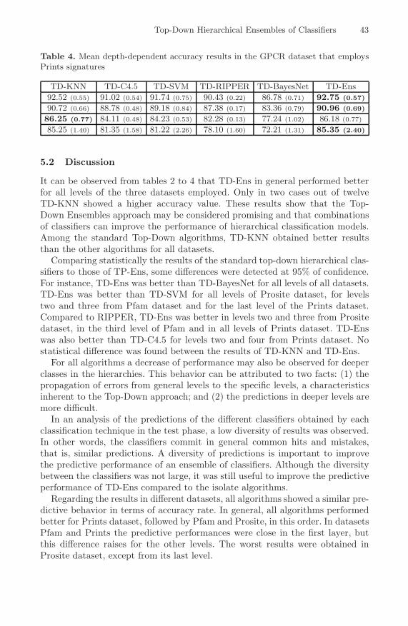
Top-Down Hierarchical Ensembles of Classifiers 43
Table 4. Mean depth-dependent accuracy results in the GPCR dataset that employsPrints signatures
TD-KNN TD-C4.5 TD-SVM TD-RIPPER TD-BayesNet TD-Ens
92.52 (0.55) 91.02 (0.54) 91.74 (0.75) 90.43 (0.22) 86.78 (0.71) 92.75 (0.57)
90.72 (0.66) 88.78 (0.48) 89.18 (0.84) 87.38 (0.17) 83.36 (0.79) 90.96 (0.69)
86.25 (0.77) 84.11 (0.48) 84.23 (0.53) 82.28 (0.13) 77.24 (1.02) 86.18 (0.77)
85.25 (1.40) 81.35 (1.58) 81.22 (2.26) 78.10 (1.60) 72.21 (1.31) 85.35 (2.40)
5.2 Discussion
It can be observed from tables 2 to 4 that TD-Ens in general performed betterfor all levels of the three datasets employed. Only in two cases out of twelveTD-KNN showed a higher accuracy value. These results show that the Top-Down Ensembles approach may be considered promising and that combinationsof classifiers can improve the performance of hierarchical classification models.Among the standard Top-Down algorithms, TD-KNN obtained better resultsthan the other algorithms for all datasets.
Comparing statistically the results of the standard top-down hierarchical clas-sifiers to those of TP-Ens, some differences were detected at 95% of confidence.For instance, TD-Ens was better than TD-BayesNet for all levels of all datasets.TD-Ens was better than TD-SVM for all levels of Prosite dataset, for levelstwo and three from Pfam dataset and for the last level of the Prints dataset.Compared to RIPPER, TD-Ens was better in levels two and three from Prositedataset, in the third level of Pfam and in all levels of Prints dataset. TD-Enswas also better than TD-C4.5 for levels two and four from Prints dataset. Nostatistical difference was found between the results of TD-KNN and TD-Ens.
For all algorithms a decrease of performance may also be observed for deeperclasses in the hierarchies. This behavior can be attributed to two facts: (1) thepropagation of errors from general levels to the specific levels, a characteristicsinherent to the Top-Down approach; and (2) the predictions in deeper levels aremore difficult.
In an analysis of the predictions of the different classifiers obtained by eachclassification technique in the test phase, a low diversity of results was observed.In other words, the classifiers commit in general common hits and mistakes,that is, similar predictions. A diversity of predictions is important to improvethe predictive performance of an ensemble of classifiers. Although the diversitybetween the classifiers was not large, it was still useful to improve the predictiveperformance of TD-Ens compared to the isolate algorithms.
Regarding the results in different datasets, all algorithms showed a similar pre-dictive behavior in terms of accuracy rate. In general, all algorithms performedbetter for Prints dataset, followed by Pfam and Prosite, in this order. In datasetsPfam and Prints the predictive performances were close in the first layer, butthis difference raises for the other levels. The worst results were obtained inProsite dataset, except from its last level.
44 E.P. Costa et al.
6 Conclusions
In this paper, we presented a comparative study of six hierarchical classificationalgorithms for different kinds of protein signatures - Prosite, Pfam and Prints.Five of the algorithms were developed according to the standard Top-Downapproach, using the following ML techniques: C4.5, RIPPER, SVMs, KNN andBayesNet. The results from these algorithms were compared with the results ofan algorithm based on a variation of the Top-Down approach named Top-DownEnsembles approach, which combines results from classifiers induced by the fiveML techniques previously mentioned.
In order to evaluate the performance of these algorithms, experiments wereperformed using three bioinformatics datasets, which are related with G-Protein-Coupled Receptors (GPCRs). Each dataset was generated based on one of thethree protein signatures considered in this work, allowing the comparison of theresults of an algorithm across different kinds of protein signatures.
According to the experimental results, TD-Ens outperformed the other algo-rithms for all datasets, with some exceptions. Therefore, the results of the Top-Down Ensembles approach may be considered promising. This indicates thatcombinations of classifiers can improve the performance of hierarchical classifi-cation models. Among the standard Top-Down algorithms, TD-KNN obtainedbetter results than the other algorithms for all datasets.
As the algorithms investigated in this work were developed to deal with classhierarchies structured as trees, strategies to extend them to the context of hier-archies structured as DAGs should be addressed in future research. Besides, theauthors plan to investigate the performance of the hierarchical approaches foroptional leaf node predictions, eliminating the restriction that the classificationsoccur in the leaf nodes only. The authors also plan to investigate the use of di-versity measures for the selection of base classifiers in the Top-Down Ensemblesapproach. Finally, it would be of great interest to investigate the use of differentkinds of protein signatures in the same dataset.
Acknowledgments. The authors would like to thank the Brazilian researchcouncils FAPESP and CNPq for their financial support and Nicholas Holden formaking available the GPCR datasets.
References
1. E. B. Institute, Protein function (accessed March 07, 2008),http://www.ebi.ac.uk/2can/tutorials/function/
2. Apweiler, R., Attwood, T., Bairoch, A., Bateman, A., Birney, E., Biswas, M.,Bucher, P., Cerutti, L., Corpet, F., Croning, M., et al.: The InterPro database,an integrated documentation resource for protein families, domains and functionalsites. Nucleic Acids Research 29(1), 37–40 (2001)

Top-Down Hierarchical Ensembles of Classifiers 45
3. Sigrist, C., Cerutti, L., Hulo, N., Gattiker, A., Falquet, L., Pagni, M., Bairoch,A., Bucher, P.: PROSITE: A documented database using patterns and profiles asmotif descriptors. Briefings in Bioinformatics 3(3), 265–274 (2002)
4. Bateman, A., Birney, E., Cerruti, L., Durbin, R., Etwiller, L., Eddy, S., Griffiths-Jones, S., Howe, K., Marshall, M., Sonnhammer, E.: The Pfam Protein FamiliesDatabase. Nucleic Acids Research 30(1), 276–280 (2002)
5. Attwood, T.: The PRINTS database: A resource for identification of protein fam-ilies. Briefings in Bioinformatics 3(3), 252–263 (2002)
6. E.Nomenclature, of the IUPAC-IUB, American Elsevier Pub. Co., New York, NY104 (1972)
7. Mitchell, T.M.: Machine Learning. McGraw-Hill Higher Education, New York(1997)
8. Freitas, A.A., Carvalho, A.C.P.F.: A Tutorial on Hierarchical Classification withApplications in Bioinformatics. In: Taniar, D. (ed.) Research and Trends in DataMining Technologies and Applications, pp. 175–208. Idea Group (2007)
9. Sun, A., Lim, E.P., Ng, W.K.: Hierarchical text classification methods and theirspecification. Cooperative Internet Computing 256, 18 p. (2003)
10. Sun, A., Lim, E.P., Ng, W.K.: Performance measurement framework for hierarchi-cal text classification. Journal of the American Society for Information Science andTechnology 54(11), 1014–1028 (2003)
11. Kuncheva, L.: Combining Pattern Classifiers: Methods and Algorithms. Wiley-Interscience, Chichester (2004)
12. Holden, N., Freitas, A.A.: Hierarchical Classification of G-Protein-Coupled Recep-tors with PSO/ACO Algorithm. In: Proceedings of the 2006 IEEE Swarm Intelli-gence Symposium, pp. 77–84 (2006)
13. Filmore, D.: It’s a GPCR world. Modern drug discovery 1(17), 24–28 (2004)14. GPCRDB, Information system for G protein-coupled receptors (GPCR) (accessed,
July 2006), http://www.gpcr.org/7tm/15. S. I. of Bioinformatics, Prosite - description (accessed March 01, 2008),
http://us.expasy.org/prosite/prosite details.html
16. Apweiler, R., Bairoch, A., Wu, C.H., Barker, W.C., Boeckmann, B., Ferro, S.,Gasteiger, E., Huang, H., Lopez, R., Magrane, M., et al.: UniProt: the UniversalProtein knowledgebase. Nucleic Acids Research 32, D115–D119 (2004)
17. Quinlan, J.R.: Induction of decision trees. Machine Learning 1(1), 81–106 (1986)18. Quinlan, J.R.: C4.5: Programs for Machine Learning. Morgan Kaufmann, San Fran-
cisco (1993)19. Cohen, W.: Fast effective rule induction. In: Proceedings of the Twelfth Interna-
tional Conference on Machine Learning, pp. 115–123 (1995)20. Cristianini, N., Shawe-Taylor, J.: An Introduction to Support Vector Machines
and other kernel-based learning methods. Cambridge University Press, Cambridge(2000)
21. Cover, T., Hart, P.: Nearest neighbor pattern classification, Information Theory.IEEE Transactions 13(1), 21–27 (1967)
22. Friedman, N., Geiger, D., Goldszmidt, M.: Bayesian Network Classifiers. MachineLearning 29(2), 131–163 (1997)
23. Venables, W.N., Smith, D.M.: The R Development Core Team, An introduction toR - version 2.4.1 (2006), http://cran.r-project.org/doc/manuals/R-intro.pdf
24. Dimitriadou, E., Hornik, K., Leisch, F., Meyer, D., Weingessel, A.: e1071: MiscFunctions of the Department of Statistics (e1071), TU Wien, 1–5 (2006)

46 E.P. Costa et al.
25. Hornik, K., Zeileis, A., Hothorn, T., Buchta, C.: RWeka: An R Interface to Weka,R package version 0.2-14, http://CRAN.R-project.org
26. Blockeel, H., Bruynooghe, M., Dzeroski, S., Ramon, J., Struyf, J.: Hierarchicalmulti-classification. In: Proceedings of the ACM SIGKDD 2002 Workshop onMulti-Relational Data Mining (MRDM 2002), pp. 21–35 (2002)
27. Nadeau, C., Bengio, Y.: Inference for the Generalization Error. Machine Learn-ing 52(3), 239–281 (2003)
28. Salzberg, S.: On Comparing Classifiers: Pitfalls to Avoid and a RecommendedApproach. Data Mining and Knowledge Discovery 1(3), 317–328 (1997)

A.L.C. Bazzan, M. Craven, and N.F. Martins (Eds.): BSB 2008, LNBI 5167, pp. 47–56, 2008. © Springer-Verlag Berlin Heidelberg 2008
A Hybrid Method for the Protein Structure Prediction Problem
Márcio Dorn, Ardala Breda, and Osmar Norberto de Souza
Laboratório de Bioinformática, Modelagem e Simulação de Biossistemas – LABIO
Programa de Pós-Graduação em Ciência da Computação - Faculdade de Informática
PUCRS, Av. Ipiranga, 6681- Prédio 32 - Sala 602, CEP 90619-900 Porto Alegre, RS, Brasil
{mdorn,abreda}@inf.pucrs.br, {osmar.norberto}@pucrs.br
Abstract. This article provides the initial results of our effort to develop a hybrid prediction method, combining the principles of de novo and homology modeling, to help solve the protein three-dimensional (3-D) structure prediction problem. A target protein amino acid sequence is fragmented into many short contiguous fragments. Clustered short templates fragments, obtained from experimental protein structures in the Protein Data Bank (PDB), using the NCBI BLASTp program, were used for building an initial conformation, which was further refined by molecular dynamics simulations. We tested our method with the artificially designed alpha helical hairpin (PDB ID: 1ZDD) starting with its amino acids sequence only. The structure obtained with the proposed method is topologically a helical hairpin, with a Cα RMSD of ~ 5.0 Å with respect to the experimental PDB structure for all 34 amino acids residues, and only ~ 2.0 Å when considering amino acids 1 to 22. We discuss further improvements to the method.
Keywords: Protein 3-D structure, ab initio prediction, homology modeling, molecular dynamics simulations.
1 Introduction
A protein molecule is a covalent chain of amino acids residues that, in physiological condition or native environment, adopt a unique three-dimensional (3-D) structure. This native structure dictates the biochemical function of the protein [1, 2].
Experiments by Anfinsen [3] demonstrated that a protein molecule when denatured, by disrupting conditions in their environment, can be re-folded to their native structure when the physiological condition is restored. Therefore, the amino acid sequence contains all of the information necessary to determine the native structure of the protein. Based on this principle, the native fold of a protein can be predicted computationally using only the physical-chemical information of their amino acids sequence. Protein folding [4] prediction is one of the greatest questions in structural bioinformatics and consists in understanding and predicting how the information coded in the amino acids linear sequence is translated into the 3-D structure of a protein.
48 M. Dorn, A. Breda, and O. Norberto de Souza
Many computational methodologies and algorithms have been proposed as a solution to this complex problem [5-8]. Bujnick [5] divide the principal approaches for protein structure prediction in two classes: de novo and comparative or homology modeling. De novo methods are further divided in two categories: ab initio and knowledge-based methods.
Ab initio methods are thermodynamics based and rely on the fact that the native structure of a protein corresponds to the global minimum of its Gibbs free energy [6]. This methodology simulates the protein conformational space using an energy function that describes the protein internal energy and its interaction with its surrounding aqueous environment. The objective is to find the global minimum of this free-energy hyper-surface which corresponds to the protein native or functional conformation [7, 9]. Stochastic and deterministic techniques such as Monte Carlo and Molecular Dynamics (MD) Simulations, respectively, are the preferred methodologies employed in ab initio prediction [7]. In contrast, knowledge-based methods utilize statistical potentials derived from analysis of folding patterns of known protein 3-D structures in databases [5]. From these statistical features target protein sequences can be predicted when no homologues are available [10]. Fold recognition via threading is the best example of this technique [6, 11].
In comparative modeling, the target sequence is aligned to the sequence of an evolutionarily related template with known 3-D structure in the Protein Data Bank (PDB) [12]. Once homology is detected, usually above the 30% identity threshold, modeling can proceed with copying of coordinates of the template or the average of multiples templates, or using the distance and torsions angles and inter-atomic distances from aligned regions from template as modeling restraints [5, 10]. Comparative modeling is therefore the most accurate prediction [5, 13].
Both methodologies have limitations: comparative modeling can only predict structures that have similar or identical sequences in a database of known structures. With de novo (ab initio methods) modeling we can obtain novel structures with new folds. However, the complexity and high dimensionality [14] of the search space, even for a small protein molecule, still makes the problem intractable [15], despite the availability of high performance computing.
The aim of this article is to describe a hybrid method we are developing for the protein structure prediction problem. In order to fasten the search for the global minimum of the potential function describing the native, functional structure of a protein we propose a hybrid method that combines the accuracy of homology modeling with a more realistic, force field based, physical-chemical description of a protein, using simulations by the MD method. In our method we split a target amino acid sequence into many short contiguous fragments and for each one of them we obtain templates with known 3-D structures. However, in contrast to most methods developed or under development, we do not use the whole fragment, but only the central amino acid main chain conformation. With these data we build an initial conformation which is then further refined by energy minimization and MD simulations.
In section 2 we detail the proposed method. Sections 3 and 4 provide a case study with results and discussions, and future work, respectively.

A Hybrid Method for the Protein Structure Prediction Problem 49
2 The Proposed Method
In this article we combine principles of de novo and comparative modeling to develop a hybrid method that explore the capacity these methods have to predict new (ab initio methods) and accurate (homology modeling) structures. Homology modeling is employed such as to reduce the search of the conformational space, but preserve the capacity of predicting novel structures.
A protein structure X can be represented in the form { }nxxxX ,,, 21 K= ,
where ix is a triplet of torsion angles [ ω (omega),φ (phi),ψ (psi)] of each amino
acid (aa) residue in the protein (Fig. 1). The set of consecutive triplets represent the internal rotations of a protein main chain.
Fig. 1. Schematic representation of a model peptide illustrating a triplet of main chain torsion angles. N is nitrogen, C and Cα are carbons and Ri is an arbitrary side-chain.ω (omega) is the
rotation about the peptide bond (C-N) and is fixed to 180º (trans).φ (phi) andψ (psi) are
rotations about the N-Cα and Cα-C bonds, respectively.
The method consists of 6 steps: (1) the target sequence is fragmented; (2) template fragments are obtained from a experimental data bank; (3) torsion angles (triplet) from the fragment central amino acid (aa) are calculated; (4) triplets are clusterized; (5) an initial conformation is build, and (6) the initial conformation is refined. These steps are detailed below:
1. Fragmenting the target sequence: In this step the target sequence X is fragmented
into many short is contiguous fragments with l aa each. A set S of contiguous
fragments, representing all possible fragments of length l , is created and represented
as { }pi ssS ,,K= , where is and ps are the first and last fragments, respectively. If
n is the number of aa in a target sequence X and l , the size of each is fragment, is
an odd value, then the number p of possible fragments obtained within the
fragmentation step is given by ( )[ ]1−−= lnp . A fragment is starts at the ith
residue and terminates at the jth residue, consisting of a set of consecutive triplets of
torsion angles{ ( ) ( ) }jjjiii ψφωψφω ,,,,,, 11 −− K . The triplet of torsion angles
is obtained only for the central amino acid of each is fragment and an odd value

50 M. Dorn, A. Breda, and O. Norberto de Souza
for l guarantees that the central aa in the fragment is flanked by an equal number o
amino acid residues. We adopt a default value of 5=l for the fragment lengths in
this work. The pseudo code for obtaining all consecutive short is fragments from a
target sequence X is:
Fragmentation (sequence, seqLength, targetSeqLength) { fragLength = 5; fragments [((seqLength)–(fragLength-1)]; end = 1; counter = 0; fragment = “”; while (end != 0) { if ((targetSeqLength-dislocate) >= fragLength) { for (i = dislocate; i < fragLength + dislocate; i++) { fragment = fragment + sequence[i];} fragments[counter] = fragment; fragment = “”; counter = counter + 1; end = 1;} else { end = 0;} dislocate = dislocate + 1;} return fragments;}
2. Searching templates using BLAST: Each of the is fragments of size l obtained
in step 1 was used to search the PDB for templates, using the web version of BLASTp for short and near exact matches [16]. Only hits with the same length as the query sequence and with no evolutionary relationship with the target sequence X were retrieved and considered in further analysis. We modified the BioPython library [17] to automate this step. The final result is a list of templates with their PDB accession codes (PDB ID).
3. Calculating triplets of torsion angles: For each target fragment is a set of template
PDB files was obtained. For every central amino acid of all is templates triplets of
torsion angles were calculated using the program Torsions (kindly provided by Dr.
Andrew C.R. Martin). Now, each is target fragment can be represented as a set of
triplet torsion angles { }ni tts ,,1 K= , obtained from all of its is templates, where it
is a triplet of torsion angles of the central aa of the templates. Hence, we may represent
the set S of fragments as { } { }{ }nipnii ttsttsS ,,,,,, KKK === .
4. Clustering the triplets: In this step all it elements belonging to one is are
clustered in order to identify in which region or regions of the Ramachandran plot [18] the triplets are more likely to be. We first generate four clusters because we consider the Ramachandran plot is divided into four major conformational regions. The first region, -180°<φ <0°, -100°<ψ <45°, is considered to be in aα -helix
conformation. The second, with -180°<φ <-45°, 45°<ψ <225° is considered to be

A Hybrid Method for the Protein Structure Prediction Problem 51
in a β -sheet region. The third, the area between 0°<φ <180°, -90°<ψ <90°, is
called the turn region, and the remaining region, representing 36% of the total area, but containing only 1.9% of the amino acids [19], is the fourth region. We utilize the EM (expectation-maximization) clustering algorithm from WEKA data
mining package [20] for processing and finding clusters in all sets of is triplet
torsion angles. The EM algorithm first calculates the clusters probabilities and, in a second step, it calculates the distribution parameters, maximizing the likelihood of the distributions given a data set [20]. For all clustering tasks a standard seed value
of 10 was used. At the end of the clustering step we had, for each is set, four
clusters, and for each one of them we had an associated mean triplet value and an estimated standard deviation (e.s.d.). In Fig. 2 we illustrate the cluster identification after running the EM algorithm. In this step we have all the information necessary to build an initial conformation for the target sequence X .
We defined the best cluster of a is set as the one with the highest number
of it elements.
Fig. 2. Ramachandran plot of all it triplets (phi, psi) of a is set. Four clusters (light blue lines) have been identified by WEKA.
5. Building the initial conformation: The mean of the triplet torsion angles from the best cluster for each aa is used to build the initial conformation of the target amino acid sequence X . We substitute the mean torsion angles of the central triplet of
each is into the target amino acid sequence X . Fragmentation with l = 5 results in
the loss of the first and last two amino acid residues. The triplet torsion angles for these four residues are obtained from the experimental structure (PDB ID: 1ZDD). The initial conformation was built with the tLeap module of AMBER7 [21]. All ω torsion angles were set to 180º since the peptide bond is partially rigid and the atoms involved are not free to rotate about it [2].
6. Refinement with MD simulation: The initial conformation build for the target sequence X was refined with energy minimization and MD simulation using the SANDER module of the AMBER7 package [21] with the Cornell el al. (22) force field.

52 M. Dorn, A. Breda, and O. Norberto de Souza
3 Case Study
To test our method we chose a mini protein composed of 34 amino acids (PDB ID: 1ZDD – Fig. 3A) [23] known to be arranged as two alpha-helices connected by a turn, a structural motif know as alpha-helical hairpin [24].
Fig. 3. Ribbon representation of the experimental and predicted conformations of 1ZDD. (A) Experimental structure of 1ZDD (PDB ID: 1ZDD). (B) Initial (green), minimized (blue) and MD simulated structure (magenta) of predicted 1ZDD. Amino acids side chains not shown for clarity.
The target sequence X = FNMQCQRRFYEALHDPNLNEEQRNAKIKSIRDDC is fragmented into 30 target short contiguous fragments with l = 5 aa (pentapeptides).
For each is fragment we performed a BLAST search for template fragments against
the PDB [12]. We removed all PDBs which had sequences similar or were identical to 1ZDD, namely: 1ZDC, 1ZDD, 1L6X, 1OQO, 1OQX, 1ZDA, 1ZDB, 2SPZ, 1LP1, 1Q2N, 1FC2, 1BDC, 1BDD, 1SS1, 1DEE, 1EDK, 1EDJ, 1EDI, 1EDL. This should eliminate any bias due to sequences of know structures but very closely related to 1ZDD.
The triplet’s torsion angles it from the templates for each target is are clustered
and its average and estimated standard deviation (e.s.d) are calculated for the φ and
ψ angles of the best cluster (cluster with most elements). The estimated e.s.d
represents the distance between the maximum and the minimum φ and ψ angles of
a given cluster. In the next page Table 1 shows the results of this analysis for the best
cluster of each is fragment.
The initial structure generated for 1ZDD (Fig. 3B, green) with our method already had a conformation similar to the expected helical hairpin found in the experimental structure (Fig. 3A). The C-terminal helix was malformed. This model was submitted to 500 steps of energy minimization to eliminate structural strains. However, only very minor changes were observed, with the minimized structure still very similar to the predicted 1ZDD. A root-mean square deviation (RMSD) of 4.9 Å was measured between the predicted 1ZDD and the experimental structure, for the main chain atoms only. When the N-terminal helix only was considered (residues 1 to 22), the RMSD was 1.9Å.

A Hybrid Method for the Protein Structure Prediction Problem 53
Table 1. The average and e.s.d of φ and ψ values for each best cluster of a is fragment
is fragment Amino Acid φ aver φ e.s.d ψ aver ψ e.s.d
FNMQC M -64.45 3.67 -39.22 8.38 NMQCQ Q -64.10 7.71 -42.44 8.47 MQCQR C -65.71 7.59 -41.19 8.67 QCQRR Q -61.78 2.70 -42.18 2.84 CQRRF R -59.89 6.78 -31.96 9.48 QRRFY R -60.98 7.48 -32.84 12.83 RRFYE F -59.73 1.82 -38.77 4.39 RFYEA Y -57.58 1.89 -46.83 5.52 FYEAL E -66.30 2.61 -42.13 3.60 YEALH A -66.32 4.33 -36.08 4.42 EALHD L -65.80 4.846 -38.77 10.35 ALHDP H -106.20 16.57 0.60 18.15 LHDPN D -75.23 15.99 122.84 13.27 HDPNL P -58.44 3.74 -35.65 22.26 DPNLN N -60.47 3.29 -22.71 6.46 PNLNE L -79.55 8.49 143.46 5.81 NLNEE N -88.70 25.87 142.92 29.48 LNEEQ E -61.78 6.21 -35.80 8.96 NEEQR E -61.88 2.57 -48.38 5.26 EEQRN Q -65.38 5.69 -46.10 5.33 EQRNA R -65.44 5.85 -40.75 5.52 QRNAK N -61.40 6.02 -44.98 5.37 RNAKI A -72.24 7.37 156.82 2.91 NAKIK K -70.54 2.51 -32.38 6.08 AKIKS I -82.52 7.93 116.37 13.62 KIKSI K -83.03 4.67 -44.76 11.53 IKSIR S -68.21 15.56 -38.22 20.86 KSIRD I -54.73 2.73 -45.87 4.21 SIRDD R -54.73 10.76 -26.08 16.99 IRDDC D -66.87 10.40 -32.10 11.07
The hairpin’s second alpha helix, at the predicted 1ZDD C-terminus, is misfolded due to hydrogen bond interactions formed between residues glutamine 22 and arginine 31 (Fig. 3B) that lead to breakage of the typical i – (i +4) hydrogen bonding pattern observed in canonical alpha helices [2].
The MD Protocol and Structural Analysis The predicted minimized conformation of 1ZDD was submitted to a further 500 ps MD simulation, at 281.0 K and a 10.0 Å cutoff radius for the evaluation of the long-range van der Waals and electrostatic interactions. The solvent was treated implicitly within the Generalized Born with Surface Area (GBSA) approximation [25]. The SHAKE algorithm [26] was used to restrain all hydrogen-heavy atom bond distances, allowing an integration time-step of 0.002 ps for the equations of motion. The simulation was performed on a PC Pentium 4 (2,4 MHz and 1GB RAM). The atomic positions were saved at every 500 steps (1.0 ps).
The secondary and supersecondary structures, as well as other structural parameters, were monitored based on the RMSD of the predicted 1ZDD MD trajectory with respect to 1ZDD.pdb, the experimental structure [23]. Structure formation was visualized with the Swiss-PdbViewer [27] and PyMol [28] graphics
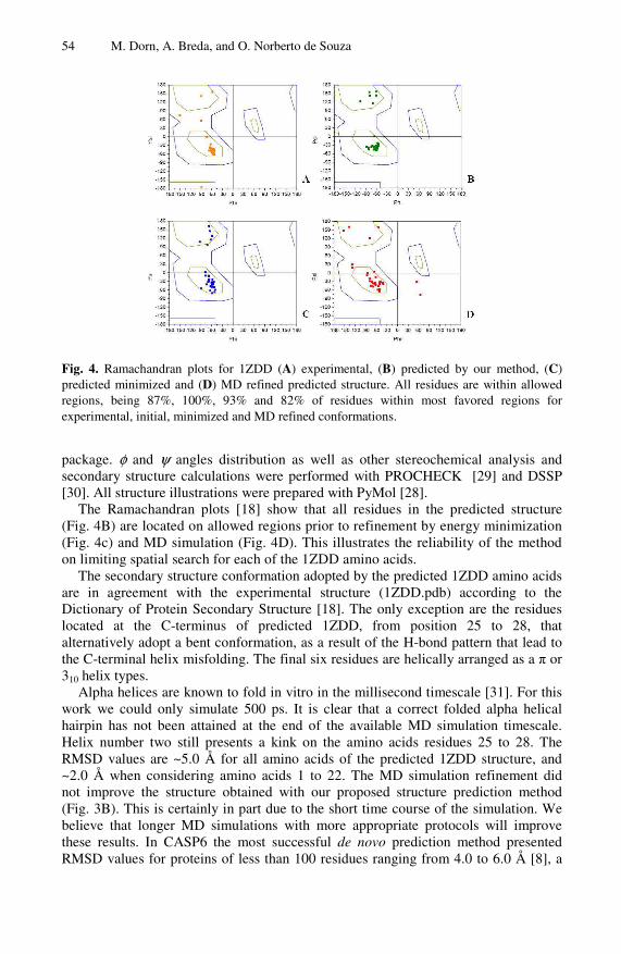
54 M. Dorn, A. Breda, and O. Norberto de Souza
Fig. 4. Ramachandran plots for 1ZDD (A) experimental, (B) predicted by our method, (C) predicted minimized and (D) MD refined predicted structure. All residues are within allowed regions, being 87%, 100%, 93% and 82% of residues within most favored regions for experimental, initial, minimized and MD refined conformations.
package. φ and ψ angles distribution as well as other stereochemical analysis and secondary structure calculations were performed with PROCHECK [29] and DSSP [30]. All structure illustrations were prepared with PyMol [28].
The Ramachandran plots [18] show that all residues in the predicted structure (Fig. 4B) are located on allowed regions prior to refinement by energy minimization (Fig. 4c) and MD simulation (Fig. 4D). This illustrates the reliability of the method on limiting spatial search for each of the 1ZDD amino acids.
The secondary structure conformation adopted by the predicted 1ZDD amino acids are in agreement with the experimental structure (1ZDD.pdb) according to the Dictionary of Protein Secondary Structure [18]. The only exception are the residues located at the C-terminus of predicted 1ZDD, from position 25 to 28, that alternatively adopt a bent conformation, as a result of the H-bond pattern that lead to the C-terminal helix misfolding. The final six residues are helically arranged as a π or 310 helix types.
Alpha helices are known to fold in vitro in the millisecond timescale [31]. For this work we could only simulate 500 ps. It is clear that a correct folded alpha helical hairpin has not been attained at the end of the available MD simulation timescale. Helix number two still presents a kink on the amino acids residues 25 to 28. The RMSD values are ~5.0 Å for all amino acids of the predicted 1ZDD structure, and ~2.0 Å when considering amino acids 1 to 22. The MD simulation refinement did not improve the structure obtained with our proposed structure prediction method (Fig. 3B). This is certainly in part due to the short time course of the simulation. We believe that longer MD simulations with more appropriate protocols will improve these results. In CASP6 the most successful de novo prediction method presented RMSD values for proteins of less than 100 residues ranging from 4.0 to 6.0 Å [8], a

A Hybrid Method for the Protein Structure Prediction Problem 55
value comparable to the results presented here, considering the full sequence, but much higher than the one we obtain when the misfolded C-terminal residues are not included in the RMSD calculation.
4 Final Considerations and Future Work
The simple protein structure prediction method we are developing was able to generate a predicted structure topologically very close to the desired one and with a processing time of only 3 minutes, after clustering of templates obtained from the PDB. This shows the method’s potential for reducing the high dimensionality of the conformational search space for a given protein sequence. At this stage, our MD simulation refinement protocol did not work. As future work to improve our method we will investigate the application of enhanced clustering techniques to the torsion angles triplets, test the effect of different clusters on the initial predicted structure, and develop better MD simulations protocols, including simulations in longer time scales and possibly using explicit salvation.
Acknowledgements
We thank the reviewers for their useful comments and suggestions to improve the original manuscript. This project was supported by grants from CAPES, FAPERGS, and CNPq to ONS. ONS is a CNPq Research Fellow. MD was supported by a CNPq M.Sc. scholarship. AB was supported by a CAPES scholarship.
References
1. Baxevanis, A.D., Ouellette, B.F.F.: Bioinformatics: A Practical Guide to the Analysis of Genes and Proteins, 560 p. Wiley and Sons, Hoboken (2005)
2. Branden, C., Tooze, J.: Introduction to Protein Structure, 410 p. Garlang Publishing Inc., New York (1998)
3. Anfinsen, C.B., Haber, E., Sela, M., White Jr., F.H.: Proceedings of the National Academy of Sciences USA. 47, 1309–1314 (1961)
4. Creighton, T.E.: Protein Folding. Biochemical Journal 270, 1–16 (1990) 5. Bujnicki, J.M.: Protein Structure Prediction by Recombination of Fragments.
Chembiochem. 7(1), 19–27 (2006) 6. Tramontano, A.: Protein Structure Prediction, 228 p. John Wiley and Sons, Weinheim
(2006) 7. Osguthorpe, D.J.: Ab initio Protein Folding. Current Opinion in Structural Biology 10,
146–152 (2000) 8. Moult, J.: A Decade of CASP: Progress, Bottlenecks and Prognosis in Protein Structure
Prediction. Current Opinion in Structural Biology 15, 285–289 (2005) 9. Tramontano, A., Morea, V.: Assessment of homology based predictions in CASP5.
Proteins: Structure, Function, and Bioinformatics 53, 352–368 (2003) 10. Kolinski, A.: Protein Modeling and Structure Prediction with a Reduced Representation.
Acta Biochimica Polonica 51, 349–371 (2004) 11. Jones, D.T., Taylort, W.R., Thornton, J.M.: A New Approach to Protein Fold. Nature 358,
86–89 (1992)

56 M. Dorn, A. Breda, and O. Norberto de Souza
12. Berman, H.M., Westbrook, J., Feng, Z., Gilliland, G., Bhat, T.N., Weissig, H., Shindyalov, I.N., Bourne, P.E.: The Protein Data Bank. Nucleic Acids Research 28(1), 235–242 (2000)
13. Marti-Renom, M.A., Stuart, A., Fiser, A., Sánchez, R., Melo, F., Sali, A.: Comparative Protein Structure Modeling of genes and genomes. Annual Review of Biophysics and Biomolecular Structure 29, 291–325 (2000)
14. Ngo, J.T., Marks, J., Karplus, M.: Computational Complexity, protein structure prediction and the Levinthal Paradox. In: Merz Jr., K., Grand, S.L. (eds.) The Protein Folding Problem and Tertiary Structure Prediction, ch. 14, pp. 435–508. Birkhäuser, Boston (1997)
15. Levinthal, C.: Are there pathways for protein folding? Journal de Chimie Physique et de Physico-Chimie Biologique 65, 44–45 (1968)
16. Altschul, S.F., Madden, T.L., Schäffer, A.A., Zhang, J., Zhang, Z., Miller, W., Lipman, D.J.: Gapped BLAST and PSI-BLAST: a New Generation of Protein Database Search Programs. Nucleic Acids Research 25, 3389–3402 (1997)
17. Chapman, B., Chang, J.: Biopython: Python Tools for Computational Biology. ACM SIGBIO Newsletter 20(2), 15–19 (2002)
18. Ramachandran, G.N., Sasisekharan, V.: Advances in Protein Chemistry 23, 238–437 (1968) 19. Hovmöller, T.Z., Ohlson, T.: Conformation of Amino Acids in Proteins. Acta
Crystallographica D58, 768–776 (2002) 20. Witten, I.H., Frank, E.: Data Mining: Practical Machine Learning Tools and Techniques,
2nd edn., 525 p. Elsevier, San Francisco (2005) 21. Case, D.A., Cheatham, T.E., Darden, T., Gohlke, H., Luo, R., Merz, K.M., Onufriev, A.,
Simmerling, C., Wang, B., Woods, R.J.: The AMBER Biomolecular Simulation Programs. Journal of Computational Chemistry 26(16), 1668–1688 (2005)
22. Cornell, W.D., Cieplak, P., Bayly, C.I., Gould, I.R., Merz Jr., K.M., Ferguson, D.M., Spellmeyer, D.C., Fox, T., Caldwell, J.W., Kollman, P.A.: A Second Generation Force Field for the Simulation of Proteins. Journal of the American Chemical Society 117, 5179–5197 (1995)
23. Starovasnik, M.A., Braisted, A.C., Wells, J.A.: Structural Mimicry of a Native Protein by a Minimized Binding Domain. Proceedings of the National Academy of Sciences USA 94, 10080–10085 (1997)
24. Murzin, A.G., Brenner, S.E., Hubbard, T., Chothia, C.: SCOP: a Structural Classification of Proteins Database for the Investigation of Sequences and Structures. Journal of Molecular Biology 247, 536–540 (1995)
25. Bashford, D., Case, D.A.: Generalized Born Models of Macromolecular Solvation Effects. Annual Review Physical Chemistry 51, 129–152 (2000)
26. Ryckaert, J.P., Ciccotti, G., Berendsen, H.J.C.: Numerical Integration of the Cartesian Equation of Motion of a System with Constraints: Molecular Dynamics of N-alkanes. Journal of Computational Physics 23, 327–341 (1977)
27. Guex, N., Peitsch, M.C.: SWISS-MODEL and The Swiss-PdbViewer: An Environment for Comparative Protein Modeling. Electrophoresis 18, 2714–2723 (1997)
28. DeLano, W.L.: The PyMOL Molecular Graphics System. DeLano Scientific, San Carlos (2002)
29. Laskowski, R.A., MacArthur, M.W., Moss, D.S., Thornton, J.M.: PROCHECK: A Program to Check the Stereochemical Quality of Protein Structures. Journal of Applied Crystallography 26, 283–291 (1993)
30. Kabsch, W., Sander, C.: Dictionary of Protein Secondary Structure: Pattern Recognition of Hydrogen-Bonded and Geometrical Features. Biopolymers 22, 2577–2637 (1983)
31. Clarke, D.T., Doig, A.J., Stapley, B.J., Jones, G.R.: The alpha-helix Folds on the Millisecond Time Scale. Proceedings of the National Academy of Sciences USA 96, 7232–7237 (1999)
A.L.C. Bazzan, M. Craven, and N.F. Martins (Eds.): BSB 2008, LNBI 5167, pp. 57–67, 2008. © Springer-Verlag Berlin Heidelberg 2008
Detecting Statistical Covariations of Sequence Physicochemical Properties
Moshe A. Gadish and David K.Y. Chiu
Department of Computing and Information Science, University of Guelph, Guelph, Ontario, N1G 2W1, Canada
Abstract. Sequence analysis often does not take the physicochemical properties into account. On the other hand, some of these properties when identified may be useful in inferring the folding and functional attributes of the molecule when considered with the original sequence information. We evaluated here an analysis using multiple aligned sequences incorporating five physicochemical properties. In addition to site invariance information, we also consider the covariation or interdependence patterns between aligned sites using an information measure. We propose a method based on analyzing the expected mutual information between sites that is statistically significant with a confidence level. When summing the measured information along the aligned sites, we compare the pattern from the measure to the structural and active site of the molecule. In the experiments, the model enzyme molecule lysozyme is chosen. The aligned sequence data are evaluated based on the mapped physicochemical properties of the amino acid residues. Analysis between the original and the transformed sequence data incorporating the physicochemical properties are then compared subtracted and visualized. From the comparisons, the plots show that some of the selected physicochemical properties in the analysis correlate to the locations of active sites and certain folding structure such as helices. The experiments generally support the useful role of incorporating additional physicochemical properties into sequence analysis, when significance of the statistical variations is taken into account.
Keywords: Physicochemical, interdependency, lysozyme.
1 Introduction
The effect of various physicochemical properties of amino acids on the protein structure and function is well known. For example, by considering the conserved physicochemical properties in addition to the amino acid types of the sequences, a meaningful alignment may be obtained. Thus, the classifier using PHYSEAN (PHYsical Sequence Analysis) adds position-specific physicochemical information for protein classification [1]. PHYSEAN predicts protein classes with highly variable sequences on the basis of their physical, chemical and biological characteristics (such as hydrophobicity). PHYSEAN produces reasonably accurate predictions, indicating the importance of incorporating the physicochemical properties into protein sequence analysis. Hydrophobicity plots have also been used in protein sequence analysis for

58 M.A. Gadish and D.K.Y. Chiu
the purpose of discovering hydrophobic cores and resolving some of the problems in protein folding. Other successes of incorporating physicochemical properties include the use of amino acid scales and physicochemical properties in predicting secondary structure propensity (alpha helix, beta sheet, turn, etc.) [2]. This paper evaluates further how these physicochemical properties can be used to analyze multiple aligned sequences of a protein family. Many speculations on why physicochemical properties in protein analysis are useful can be made. Proteins have remarkable range of functions from the many distinctive three-dimensional structures given their sequences [3]. Sequence analysis may determine how the amino acids specify the conformations of their structure. An important step in analyzing the sequences then involves finding recurrent patterns in the sequence that may not be obvious. From these patterns, relationship to patterns of the function of the protein can then be analyzed [4]. Information measures such as the Shannon entropy function or mutual information are mathematical measures that are general and may reveal implicit statistical relationships even though the exact properties that are involved may be unknown. Crooks and Brenner [5] have used entropy densities and local inter-sequence mutual information density to study the effect of primary and secondary protein structure. A transformation score is mapped from each amino acid into the three secondary structure classes of extended beta sheets, helices, and loops. Their study supports the view that these information measures may capture the cooperative processes where secondary and tertiary structure can then form.
This paper develops a method by analyzing the statistical significance of expected mutual information based on the physicochemical properties. It further sums all such mutual information at each position and compares it to that without taking the physicochemical properties into account. The plots showing the differences are then evaluated.
In the experiments, the model enzyme molecule lysozyme c is chosen. The aligned sequence data are evaluated based on the mapped physicochemical properties of the amino acid residues. Analysis between the original and the transformed sequence data incorporating the physicochemical properties are then compared and visualized. From the comparisons, the plots show that some of the selected physicochemical properties correlate to the locations of active sites and certain folding structure. The experiments generally support the interesting role of these physicochemical properties when their statistical variations are taken into account.
2 Detecting Significant Interactions between Sites
2.1 Representation of Aligned Sequence Data
Multiple biological sequences (of a protein family) can be aligned to form a sequence ensemble. For example, each amino acid site in the protein sequence can be considered as a variable where the corresponding amino acid of a sequence is the outcome. This can be represented as X = (X1, X2,…, Xm) where m is the number of variables, indicating the length of the alignment. An instance of X is a realization denoted as x=(x1,x2,…,xm). Each (1 )jx j m≤ ≤ can take up an attribute
value denoted as j jqx a= . An attribute value jqa is a value taken from an attribute

Detecting Statistical Covariations of Sequence Physicochemical Properties 59
value set Γj = { jqa │q = 1,2, …, Lj} where Lj is the number of possible values for the variable Xj, or the cardinality of the set.
2.2 Expected Mutual Information
Expected mutual information is a measure of the statistical interdependence between two random variables. The stronger the interdependence between the two variables, the larger is the expected mutual information between them. If the two variables are independent, then the expected mutual information between them is zero [6], [7], [8]. Intuitively, expected mutual information measures the amount of information associated between the two variables. Quantitatively, it can also be considered as the distance between the joint distribution of two variables, and their joint distribution if they were independent.
Formally, the expected mutual information of two discrete random variables Xi and Xk can be defined as,
1 1
( , ) ( , ) log( , )
( ) ( )
LLi kj h
i kj h
j hi k
i k j hi k
I X X p x xp x x
p x p x= =
=∑∑ . (1)
where j
ix and h
kx are the jth and hth outcome of iX and
kX respectively.
2.3 Testing for Statistical Interdependence
It is important when calculating statistical interdependence to take into consideration their statistical significance, so that their correspondence is not due to chance, otherwise considerable error can be accumulated. This is especially important in case when information from multiple variables is summed. Evidence of statistical interdependence can be evaluated by comparing the two competing hypothesis between the independence and interdependence assumptions.
When comparing the statistical independence between two outcome values of the distinct variables, we use the following method based on evaluating the adjusted residual [8]. Let us denote a joint outcome of the two variables Xi and Xk
as ( , )jh j h
ik i ke a a= , where jh
ike represents the joint observation of j
iiX a= and h
kkX a= .
The standard residual is defined as:
( ) ( )( )
( )
jh jhjh ik ik
ikjh
ik
obs e exp ez e
exp e
−= . (2)
Here, ( )jh
ikobs e is the observed frequency and ( )jh
ikexp e is the expected frequency for
the joint observation jh
ike in the sequence ensemble. The adjusted residual is defined
as [8]:
( )( )
( )
jhjh ik
ikjh
ik
z ed e
v e= . (3)

60 M.A. Gadish and D.K.Y. Chiu
where,
( ) (1 ( ))(1 ( ))jh
ik
j hi i k kv e P X a P X a= − = − = . (4)
The adjusted residual, ( )jh
ikd e , has an asymptotic normal distribution. Hence, by
convention, a statistical significance level of either 95% or 99% can be chosen. Using a 2-tailed test, the corresponding tabulated threshold values are 1.96 and 2.58, respectively. We define a statistically significant event as a joint observation, that is, the two values being statistically interdependent as,
( )jh
ikd e Nα> (5)
where Nα is the threshold value with a statistical significance level α.
2.4 Significant Expected Mutual Information
A measure of expected mutual information involving only the significant events in the variable-pair can be denoted as I*(Xi,Xk). Expected mutual information I*(Xi,Xk) as defined in Eq.1 subjected to the selections from the statistical test, as derived in Eq.3, can be denoted as:
such that * ( , ) ( , ) ( )jh
i k i k ikI X X I X X d e Nα= > . (6)
This measure of expected mutual information then calculates the significant expected mutual information of events only if they are selected to be statistically significant, with an adjusted residual value greater then a tabulated threshold with a statistical significance level α. Residual analysis identifies events that deviate from statistical independence. Thus, only those joint observations that are statistical associated will be added to the overall expected mutual information summation. In doing so, those events that are determined as statistically independent will be discarded.
Significant expected mutual information, I*(Xi,Xk), can be normalized to produce values between 0 and 1 by dividing it to Shannon entropy involving only those events. Shannon entropy involving the significant selected events is calculated as follows:
such that*( , ) ( , ) log ( , ) ( )i kL L
j h j h jh
i k i k i k ikj h
H X X p x x p x x d e Nα= − >∑∑ . (7)
The normalized expected mutual information based on the selected significant events, can now be defined as:
1* ( , )
0 * ( , )* ( , )
i ki k
i k
I X XR X X
H X X≤≤ = . (8)
To evaluate the total amount of interdependency expressed on a given variable Xi (or site on the aligned sequences) induced by the detection of R*, it can be calculated as:

Detecting Statistical Covariations of Sequence Physicochemical Properties 61
1
*( , )( )m
i i kk
R x xMR X=
=∑ (9)
This measure allows us to determine which aligned locations share large bits of information with others and those which share little.
2.5 Detecting Biosequence Interactions Using Significant Expected Mutual Information
To incorporate amino acid properties into protein sequence analysis, we substitute identified physicochemical properties into the corresponding amino acids. The aligned sequences are then transformed, and discretized into different pre-defined intervals for evaluation. The transformed sequences are then analyzed for their statistical interdependency from these discretized physicochemical properties. This method allows analysis on discrete and continuous physicochemical properties. It can also handle patterns due to non-linear and linear dependency. The physicochemical properties of different amino acid types sharing similar characteristics can then be compared and analyzed.
For physicochemical properties that have continuous value (such as molecular weight here), a scheme is developed to discretize the property. After discretization, each amino acid is substituted with its corresponding calculated label for that property. Each continuous physicochemical property is divided into n equal intervals,
max - minInterval
n= (10)
where max and min are the maximum and minimum values respectively an amino acid has for that property, and Interval is the interval size. Each property then falls into one of the predefined n intervals. Amino acids that share similar physicochemical values fall into the same interval are assigned identical discrete values. This process is repeated for each physicochemical property, producing a transformed sequence ensemble for each property, with a specified accuracy of discretization.
Significant expected mutual information can be compared between that from the original sequence ensemble and the sequences transformed from the physicochemical properties.
* *( , ) ( , ) ( , )Difference i k original i k physicochemical i kR X X R X X R X X= − (11)
The difference can be visualized along the aligned position of the sequences that reflects the summation from all positions. Each generated plot is visualized in two ways. First, the plot shows the value of significant expected mutual information (normalized) between every pair of sites in the sequence. Second, a plot can be done to visualize the cumulative significant expected mutual information, denoted by the value of MR(Xi) between a variable Xi and the other variables in the alignment.
From the plot, a high score reflects strong interdependencies between sites. Furthermore, clusters (regions with similar characteristics) can also be observed. Because of the transformation and analysis of the differences between the original and the

62 M.A. Gadish and D.K.Y. Chiu
transformed sequences, the strong interactions can be attributed to the physicochemical property being displayed.
3 Experiments
3.1 Experimental Data
The sequence ensemble consists of 75 complete lysozyme c sequences. The aligned protein sequences have 130 residues. Lysozyme c was chosen because of its qualities as a model protein. It is classified as a monomer (or protein with a single amino acid chain). This simplifies the analysis by eliminating interactions among amino acids of different peptide chains as in more complex polymeric proteins. In addition, lysozyme c lacks any cofactors or prosthetic groups, thus eliminates interactions due to these groups. Lysozyme c has been well studied and its structure and function is reasonably understood [9].
Five physicochemical properties were chosen here: polarity, hydrophobicity [10], molecular weight, molar refractivity [2] and bulkiness [11]. The polarity property is represented as discrete values. It can be broken down into six distinct values [12], [13]. Hydrophobicity, molecular weight, molar refractivity and bulkiness are all continuous values. They are each discretized using different number of intervals, n=4, 5, 6, 7, 8, for evaluation.
3.2 Experimental Method
Initialy, we calculate the value of significant expected mutual information on the original aligned sequences between sites. Since the alignment has 130 sites, it forms a 130 by 130 matrix of the R*(Xi, Xk) value. Next, these values calculated from the original sequence are compared to those from each of the five physicochemical properties based on their different discretized labels. The calculated interdependency between all positions is summarized in Table 1. Three classes of patterns were discovered in the analysis, labeled as: gap, peak, and cluster. Gap in the plots refers to a region in the sequence with low cumulative significant value. (In the plot, they are identified as horizontal and vertical white color coded bands.) The positions that are located within the gaps are often conserved with respect to the property considered. A peak in the plots reflects positions that have high cumulative significant values (indicative of strong interdependency.) A cluster is an area in the plot that represents at least one position having strong value with another region (with a length of more than one site).
3.3 Experimental Results
A comparison of different physicochemical effects on the sequence can be visualized (Fig.1, Table 1). Bulkiness and hydrophobicity have the weakest effect; while polarity has the clearest, peaked at position P76. Hydrophobicity and to a lesser extent bulkiness, display clear gaps across the sequence. Gaps are indicative of lack of the effect due to the physicochemical property. Some gaps overlap between plots (Table 2). Overlapping indicates a combined effect of the physicochemical properties

Detecting Statistical Covariations of Sequence Physicochemical Properties 63
Table 1. Patterns from the plots after subtracting the values of R* from the original sequences (extracted from Fig.1)
Site Pol Hydro Bulk MW MR P10-12 Cluster P25 Peak Peak Peak, Cluster Peak P26 Peak Peak, Cluster P27 Peak, Cluster P28 Gap Peak P29-31 Gap P41 Peak Cluster P42 Peak Peak Peak, Cluster Peak P43 Peak, Cluster P44 Peak Cluster P45-47 Cluster P53-56 Gap Gap Gap P57 Gap Gap P58-60 Gap Gap Gap P61 Peak Peak P62 Peak P65-67 Peak, Cluster P69 Peak P76 Peak P86-87 Peak, Cluster P95-97 Gap Gap P98-99 Gap P100 Peak P101-4 Gap P105 Peak Peak Peak P121 Peak P124 Peak Pol polarity, Hydro hydrophobicity, Bulk bulkiness, MW molecular weight, MR molar refractivity.
at these positions. Gaps that overlap among properties correspond to regions in the aligned sequences that are not affected by the physicochemical properties (e.g. hydrophobicity and bulkiness).
Some of the gaps include amino acids that are located in the secondary structural regions. The gap at positions P53 – P59 includes amino acids that line up with the active site cleft, in positions P57 – P59 [9]. The gap at positions P79 – P81 includes amino acids that form part of a 310 helix (a helix structure that is characterized by shorter turns then found in an α-helix) [14]. Molecular weight, molar refractivity and polarity are more irregular than hydrophobicity and bulkiness in terms of distribution of peaks and gaps in their cumulative plots. Additionally, many peaks overlap between bulkiness, molecular weight and molar refractivity. These overlapping positions show strong interactions with respect to the property being displayed. There

64 M.A. Gadish and D.K.Y. Chiu
Polarity
Aligned sequence position (x)
MR(
x)
Hydrophobicity
Aligned sequence position(x)
MR(
x)
Bulkiness
Aligned sequence position(x)
MR(
x)
Molecular Weight
Aligned sequence position(x)
MR(
x)
MolarRefractivity
Aligned sequence position(x)
MR(
x)
Fig. 1. Plots of MR(X) calculated as the differences from that of the original sequences among the 5 physicochemical properties. Interval size for molecular weight and hydrophobicity is 8; bulkiness is 5; and refractivity is 4.
are two possible explanations. It is possible that at these positions all three properties interact together, in synergy. Alternatively, the similarity between these plots can be possibly attributed to the close relationship between these three properties. For ,

Detecting Statistical Covariations of Sequence Physicochemical Properties 65
Table 2. Consistent patterns observed from the selected physicochemical properties
Physicochemical Properties Pattern Type Site Characteristics of the molecule
Hydrophobicity, Bulkiness Gap P26 – P33 Inside α-helix at positions P25 – P36.
Hydrophobicity, Bulkiness Gap P53 – P59 Inside the active site cleft P57 – P59.
Hydrophobicity, Bulkiness Gap P79 – P81 Part of a single-turn 310 helix P80 – P83, and half of the disulfine bridge between P64-P80.
Hydrophobicity, Bulkiness Gap P95 – P97 Positions are inside α-helix in P89 – P100.
Hydrophobicity, Bulkiness Gap P104 – P109
Overlap P104, P108 – P109 active site cleft.
Bulkiness, Molecular weight, molar refractivity
Peak P25 Inside and start of α-helix P25 – P36.
Bulkiness, Molecular weight, molar refractivity
Peak P41, P44 P44 is in the active site.
Molecular weight, molar refractivity
Peak P65 – P67 Near positions P63 – P64 that are in the active site. Also next to P64 which is part of a disulfide bridge (P64-P80). Possible stability role.
Bulkiness, Molecular weight, molar refractivity
Peak P105 In the active site.
instance, molecular weight, bulkiness and molar refractivity are all alternate measures of amino acid size. The peak at position P44 is the active site, while peaks at positions P41, P65 – P67 are close to it [9]. Locations that are close to active site may be accounted from the shape of the catalytic site. Positions P105 is observed to interact with several other positions in the sequence (P25, P41) with respect to bulkiness and molecular weight. Positions P105 and P41 are located in the active site, while positions P105 and P25 are spatial neighbors in the 3-Dimensional model.
3.3.1 Physicochemically Invariant Patterns It is generally agreed that the amino acid sequence of protein when considering the physicochemical properties hold important information about the protein [15].
66 M.A. Gadish and D.K.Y. Chiu
Lysozyme, when considering all the occurrences by a wide variety of organisms, provides a unique opportunity to examine the common relationship between its sequences and the other relevant information of the molecule such as structure, folding characteristics and evolutionary relationships. Lysozyme c sequences highly vary with respect to sequence similarity. For example, human and chicken lysozyme, show differences in 51 sites. However, they are structurally similar [16]. Although they exhibit differences in their amino acid values, many of the variant sites are actually invariant with respect to some physicochemical properties. Many of these invariant patterns are identified by the gaps in this study.
4 Conclusion
The experiments showed that the selected physicochemical properties have an effect on the biosequence and can be measured using the proposed significant expected mutual information. This information measure reflects an underlying pattern of interactions. Some of these patterns are located at the active sites while others are located in the secondary structural elements like helices. Many of the identified patterns are spatial neighbors that congregate sequentially. The research shows the importance of eliminating statistical variations that are not significant and focusing on events that are, thus resulting in a more accurate calculation in very noisy sequence data.
Acknowledgements. The research is supported by the Discovery Grant of the National Science and Engineering Research Council of Canada and the Korea Research Foundation Grant (KRF-2004-042-C00020).
References
1. Ladunga, I.: PHYSEAN: PHYsical Sequence Analysis for the identification of protein do-mains on the basis of physical and chemical properties of amino acids. Bioinformatics 15(12), 1028–1038 (1999)
2. Jones, D.D.: Amino acid properties and side-chain orientation in proteins: a cross correlation approach. J. Theor. Biol. 50(1), 167–183 (1975)
3. Branden, C., Toolze, J.: Introduction to Protein Structure, 2nd edn. Garland Publishing (1999)
4. Stolorz, P., Lapedes, A., Xia, Y.: Predicting protein secondary structure using neural net and statistical methods. J. Mol. Biol. 225(2), 363–377 (1992)
5. Crooks, G.E., Brenner, S.E.: Protein secondary structure: entropy, correlations and prediction. Bioinformatics 20(10), 1603–1611 (2004)
6. Haberman, S.J.: The analysis of residuals in cross-classified tables. Biometrics 29, 205–220 (1990)
7. Li, W.: Mutual Information Functions Versus Correlation Functions. Journal of Statistical Physics 60(5-6), 823–837 (1990)
8. Wong, A.K.C., Wang, Y.: High-order pattern discovery from discrete-valued data. IEEE Trans. Knowledge and Data Eng. 9(6), 877–893 (1997)
9. Jolles, P.: Lysozymes: Model Enzymes in Biochemistry and Biology (1996)

Detecting Statistical Covariations of Sequence Physicochemical Properties 67
10. Eisenberg, D., Schwarz, E., Komarony, M., Wall, R.: Analysis of membrane and surface protein sequences with the hydrophobic moment plot. J. Mol. Biol. 179(1), 125–142 (1984)
11. Zimmerman, J.M., Eliezer, N., Simha, R.: The characterization of amino acid sequences in proteins by statistical methods. J.Theor. Biol. 21(2), 170–201 (1968)
12. Darnell, J., Lodish, H., Baltimore, D.: Molecular Cell Biology. Scientific American Books 13. Lesk, M.A.: Introduction to Protein Architecture: The Structural Biology of Proteins.
Garland Publishing (1999); 2nd edition(1990) 14. Iyer, L.K., Qasba, P.K.: Molecular dynamics simulation of a-Lactalbumin and calcium
binding c-type lysozyme. Protein Engineering 12(2), 129–139 (1999) 15. Phillips, D.: The Hen-White Lysozyme Molecule. Proceedings of the National Academy of
Sciences of the United States of America 57, 483–495 (1967) 16. Hooke, S.D., Radford, S.E., Dobson, C.M.: The Refolding of Human Lysozyme: A
Comparison with the Structurally Homologous Hen. Biochemistry 33(19), 5867–5876 (1994)

A.L.C. Bazzan, M. Craven, and N.F. Martins (Eds.): BSB 2008, LNBI 5167, pp. 68–78, 2008. © Springer-Verlag Berlin Heidelberg 2008
Molecular Models to Emulate Confinement Effects on the Internal Dynamics of Organophosphorous Hydrolase
Diego E.B. Gomes1, Roberto D. Lins2, Pedro G. Pascutti1, Tjerk P. Straatsma2, and Thereza A. Soares2
1 Instituto de Biofísica Carlos Chagas Filho, Universidade Federal do Rio de Janeiro, RJ 21949-900, Brazil
2 Computational Science and Mathematics Division, Pacific Northwest National Laboratory P.O. Box 999, MSIN K7-90, Richland, WA 99352
Abstract. The confinement of the metalloenzyme organophosphorous hydrolase in functionalized mesoporous silica (FMS) enhances the stability and increases catalytic specific activity by 200% compared to the enzyme in solution. The mechanism by which these processes take place is not well understood. We have developed macroscopic and coarse-grain models of confinement to provide insights into how the nanocage environment steers enzyme conformational dynamics towards enhanced stability and enzymatic activity. The structural dynamics of organophosphorous hydrolase under the two confinement models are very distinct from each other. Comparisons of the present simulations show that only one model leads to an accurate depiction of the internal dynamics of the enzyme.
Keywords: phosphotriesterase, functionalized nanoporous support, enzyme im-mobilization, atomistic molecular dynamics, enhanced catalytic activity.
1 Introduction
Organophosphorous compounds are potent synthetic substances used exclusively as pesticides and chemical warfare agents (e.g. sarin, soman, VX). Due to the high toxicity and widespread use of these compounds, there is an increasing interest to develop strategies for their detection and detoxification.1 Recent breakthroughs in sensory technology have enabled the development of recyclable enzyme-based biosensors, through their confinement within nanomaterials [1, 2]. The bacterial enzyme organophosphorous hydrolase (OPH; EC 3.1.8.1) is an excellent candidate to be immobilized within biosensors due to their unique ability to catalytically detoxify organophosphorous compounds. OPH is a homodimeric (α/β)8-barrel containing an active site with two divalent metal ions which are bridged by a water molecule and a carbomoylated lysine residue Figure 1). Zn+2 is the apparent native metal, but substantial activity is observed after substitution of the binuclear metal center by Co2+, Cd2+, Mn2+, or Ni2+ [3, 4]. Both metals ions are required for full catalytic

Molecular Models to Emulate Confinement Effects on the Internal Dynamics 69
Fig. 1. Representation of two confinement models for organophosphorous hydrolase (OPH). In the positional constraint model, the N⎛ atoms of lysine residues (in CPK) are harmonically constrained (except for the carbamylated Lys169 in the active site). In the coarse-grain model functional groups COO- of the FMS pore are represented by van deer Waals spheres in red. The substrate soman is shown in ball-and-stick and Zn2+ ions in van deer Waals spheres in blue.
activity, and the kinetic constants, kcat and kcat/KM, are dependent upon the identity of the specific metal cations within the active site. OPH catalyzes the cleavage of P-O, P-F, and P-S bonds in a variety of organophosphate triesters and related phosphonates with a high catalytic turnover and broad substrate specificity [5]. Remarkably, the immobilization of OPH in functionalized mesoporous silica (FMS) was shown to enhance stability and increase enzyme catalytic activity by 200% compared to OPH free in solution [2].
The stabilization of proteins through confinement has been extensively studied through experimental and computational techniques [2, 6-16]. Based on concepts of statistical mechanics and polymer physics, confinement-induced stabilization of proteins has been attributed to a restriction of the configurational space for denatured states, i.e., reduction of the entropy of the unfolded state[12, 14]. Yet, the effect of confinement on the catalytic activity of enzymes remains less understood. In part, this is because a detailed investigation of chemical reactions requires the knowledge of its electronic structure, i.e., a quantum mechanical description. This finer level of description demands a much larger computational cost than the minimalist models traditionally used to study the effect of confinement on folding and stability of proteins [15-18]. Therefore, it imposes severe restrictions on the length and time scale of the systems to be simulated.
In order to calculate enzymatic rates for FMS-confined OPH in explicit solvent, it is desirable to emulate pore properties relevant for enzymatic activity while increasing only minimally the size of the system. Since the FMS pore is a rigid and mostly inert scaffold, it is assumed that these properties can be adequately described by a macroscopic and/or coarse representation of the pore. Indeed, a macroscopic model has
70 D.E.B. Gomes et al.
been previously used to simulate in a confined environment [6]. We have investigated this approximation by carrying out molecular dynamics (MD) simulations of the free and FMS-confined OPH in explicit solvent. The effect of the FMS pore has been emulated either as a non-atomic model [6] or as a coarse-grained model. Recently, it has also been shown that OPH mutants with distinct catalytic efficiency exhibit distinct structural dynamics [19]. Therefore, a realistic representation of the confinement environment must account for these differences. The structural dynamics of OPH under the two confinement models are very distinct from each other. Comparisons of the present simulations show that one model leads to an inaccurate depiction of the internal dynamics of OPH.
2 Computational Methodology
2.1 OPH Model
The molecular model of the enzyme OPH was built from crystallographic coordinates of the structure determined at 1.9 Å resolution (PDB code 1EZ2) [20]. Atoms are represented by a van der Waals atomic model containing atom-centered point charges to mimic the partial charge of atoms in the system. The AMBER force field was used to treat bonded and non-bonded interactions. The co-crystallized diisopropylmethyl phosphonate analog in the X-ray structure was replaced by the SpSc-soman enantiomer. Amino acid protonation states were assigned accordingly to a pH of 7.0. Zinc ions in the active site of the enzyme were treated using a non-bonded model with a formal charge of +2. Partial atomic charges and parameters for soman and the carbamylated Lys169 were calculated as described by Soares et al. 2007.
2.2 FMS Model
The interactions between OPH and the FMS have two components: steric due to the inert nature of the silica material, and electrostatic due to functionalization of the mesopore. We assume that i. steric interactions can be approximated by a non-atomic model where the positions of atoms N⎛ lysine residues are harmonically constrained (except for the carbamylated Lys169). Lysine side-chains were chose because these residues are the linkage sites in covalently linked OPH-FMS complexes [9]. Furthermore, this model was successfully used to study the confinement of beta-galactosidases by Bismuto and coworkers [6]; ii. electrostatic interactions can be modeled as a cylindrical, uniform array of atoms, each atom corresponding to a given functional group. This coarse-grain model incorporates the atomic attributes (van der Waals and coulomb parameters) characteristic of the functional group in consideration [10] derived from the AMBER force field [21]. Hence, in the case of the functional group COO-(CH2)n experimentally used to functionalize the mesoporous silica, the pore surface was represented by point charged particles with the charge number of -1 and van der Waals parameters corresponding to a carboxylate

Molecular Models to Emulate Confinement Effects on the Internal Dynamics 71
anion. These particles can be spaced apart to reproduce the percentage of functional group coverage (1 nm for 20% coverage) [2]. The OPH structure was docked to the FMS pore wall based on the complementarity of their electrostatic potential surfaces calculated with the program APBS [22].
2.3 MD Simulations Setup
MD simulations were carried out for OPH free in solution (OPHfree), OPH confined through atom positional constraints (OPHfix) and through the coarse-grain representation of the FMS pore (OPHfms). For the sake of conciseness, a brief description of computational methods is presented here. For more details see [19, 23, 24]. Runs were performed under a NPT ensemble with a time step of 1fs during the equilibration and 2 fs during the production runs. The temperatures of solute and solvent were controlled by separately coupling them to a Berendsen thermostat with a relaxation time of 0.1 ps. The pressure was maintained at 1.025 x 10⁵ Pa by means of isotropic coordinate scaling with a relaxation time t = 0.4 ps. A time step of 2 fs was used to integrate the equations of motion based on the leapfrog algorithm. The bond lengths between hydrogen and heavy atoms were constrained by using the SHAKE algorithm with a tolerance of 10-3 nm. A short-range cutoff of 1.0 nm was used for all non-bonded interactions, and long-range electrostatic interactions were treated by the smooth Particle Mesh Ewald method. The equilibration procedure consisted of thermalization of the solvent, with the solute atoms fixed, for 20 ps at 298.15 K, followed by minimization of all solute atoms, keeping the solvent coordinates fixed, and then simulation of the complete system by raising the temperature from 0 to 298.15 K in 20 ps increments of 50 K each of MD simulation. Data production was carried out for 5 ns and configurations of the trajectory were recorded every 0.2 ps. Within modest simulation times of 5 ns, several structural properties, including backbone RMSD, have reached convergence. All simulations were performed with the NWChem program [25] and the analyses of molecular trajectories were carried out with the Gromacs program [26].
3 Results
3.1 Structural Stability
Atom-positional root-mean-square deviations (RMSD) were determined for backbone atoms in the MD trajectories with respect to their positions in the X-ray structure (Figure 2). The RMSD profiles of OPHfree and OPHfms are comparable but significantly distinct from that of OPHfix. The RMSD for the OPHfix simulation displays values of 0.07-0.08 nm (+/- 0.005 nm) early after the equilibration phase and remains as such throughout the entire trajectory. In contrast, the RMSD for both OPHfree and OPHfms converged after ca. 4 ns to values between 0.12-0.15 nm (+/- 0.013 nm).

72 D.E.B. Gomes et al.
Fig. 2. Root-mean-square deviation of backbone atoms of OPHfree (free), OPHfix (fix) and OPHfms (FMS) with respect to the X-ray structures 1EZ2[20]
3.2 Structural Dynamics
The effect of the confinement models on internal dynamics of OPH can be inferred by comparisons of the atom-positional RMS fluctuations (RMSF) and essential dynamics (ED) for OPHfree, OPHfix and OPHfms. The RMSF of backbone atoms were calculated for OPHfree, OPHfix and OPHfms with respect to the X-ray structure (Figure 3). The three simulations exhibit average atomic fluctuations below 0.03 nm, with average RMSF values of 0.06 nm ± 0.02 for OPHfree and OPHfms, and 0.05 ± 0.02 for OPHfix. The RMSF profiles are equivalent for the three systems except for the region corresponding to residues 165 to 180, which have much lower flexibility in OPHfix.
Fig. 3. Root-mean-square fluctuations of backbone atoms of A) OPHfree, B) OPHfix and C) OPHfms with respect to the X-ray structures 1EZ2

Molecular Models to Emulate Confinement Effects on the Internal Dynamics 73
Fig. 4. Top panel: Magnitudes of eigenvalues calculated from the covariance matrix of backbone atom coordinates corresponding to the MD simulations of OPHfree, (circle) OPHfix (square) and OPHfms (triangle). Bottom panel: Eigenvector components for atomic displace-ment along the first eigenvector for the MD-generated ensembles of A) OPHfree, B) OPHfix and C) OPHfms.
ED analysis techniques were applied to the MD trajectories to separate internal motions into orthogonal motions [27]. Large-amplitude motions of the protein are described by a few eigenvector modes and separated from a much larger number of remaining small-scale motions. The technique is based on the diagonalization of the covariance matrix of atomic fluctuations obtained from the MD trajectories, after removal of overall translation and rotation [27]. The eigenvalues are the average square displacements and, consequently, a measure of the amplitude of the motions along the corresponding eigenvectors.
The contributions of the backbone atoms to the first and second eigenvectors are displayed in Figure 4. They represent the relative displacement of each residue due to the motion described by a given eigenvector. The anharmonic motions of OPH in the

74 D.E.B. Gomes et al.
all three simulations are described by a few eigenvector modes with most of the atomic displacement given the first and second eigenvalues (Figure 4-top). Together, the first and second eigenvectors account for 30%, 23%, and 28% of the total atom displacement in OPHfree, OPHfix and OPHfms, respectively.
4 Discussion
MD simulations of free and confined OPH structures reveal distinct dynamical and structural behaviors for OPHfix compared to OPHfree and OPHfms. First, OPHfix exhibits comparatively low and constant RMSD values. In this simulation, the ensemble of structures is conformationally more homogenous and more similar to the X-ray conformation than in OPHfree and OPHfms. Second, OPHfix shows significantly lower atomic fluctuations along the loop region corresponding to residues 170-180. Third, anharmonic motions for OPHfix have much lower amplitudes and broader distribution than for OPHfree and OPHfms. How can these dissimilarities be rationalized to allow the choice of the most realistic, yet computationally affordable, confinement model?
The differences in the atom-positional RMSD of OPHfix and the other two simulations suggest that the positional constraint model reproduces more accurately the reduced conformational space of immobilized enzymes than the coarse-grain model. However, this model also suppresses the flexibility of the loop residues 170-180 due to the harmonic constraint applied to the N⎛ atom of Lys175. This loop region is located in the entrance of the active site and contains the carbamylated Lys169 that coordinates the Zn2+ cations required by OPH for full catalytic activity. Therefore, the region is thought to play a role in the dynamics of binding and possibly catalysis of the substrate by OPH. This is corroborated by previous simulations showing that the loop region is more flexible in the substrate-bound OPH than in the unbound form [19]. In addition, experimental studies have shown that the specific activity of entrapped OPH is governed by the orientation of the enzyme in the FMS pore that in turn is determined predominantly by electrostatic interactions between the positively-charged enzyme and the negatively-charged FMS [10]. OPH shows a positive electrostatic potential spread over the surface opposed to the active site (Figure 5). The most favorable binding orientation of OPH to the electronegative pore-wall surface is via this “back” region. In such orientation the active site and residues 170-180 faces the center of the pore and are away from the functionalized groups of the pore wall. Therefore, Lys175 and neighboring residues should be under minimal steric influence of the FMS pore wall. These findings strongly suggest that the lower atomic fluctuations of residues 170-180 are an artifact introduced by the atom positional constraints.
ED analyses of MD trajectories provide insight into the persistent motions of the protein in the equilibrated state as sampled in the computer simulation. These motions need not correspond to the relevant motions required for the function of the protein, but offer a quantitative means to compare large-scale motions from different simulations. The highest-amplitude anharmonic atomic displacement represented by the eigenvalues is considerably lower for OPHfix (0.31 nm2) compared to OPHfree (0.50 nm2) and OPHfms (0.57 nm2) (Figure 4-top). The regions of the protein chiefly contributing to these motions are evident for OPHfree and OPHfms (Figure 4-bottom).

Molecular Models to Emulate Confinement Effects on the Internal Dynamics 75
Fig. 5. Representation of the electrostatic potential distribution on the molecular surface of OPH. A) Front. View (black arrows highlight the two active sites. B) Back view (which faces the FMS pore wall). Blue color represents a positive potential, red color represents a negative potential and the white color indicates areas of a neutral potential. The scale of the surface potential is given in kBT and in the range between -5 to 5 kBT.
In contrast, the same regions are nearly indistinguishable from regions contributing only marginally to anharmonic motions in OPHfix. Thus, it indicates that the positional constraint model suppresses the conformational fluctuations of the whole enzyme in a non-selective fashion. This is clearly not a realistic representation of confined OPH. Enzymatic reactions intrinsically involve multiple kinetic steps, complex protein-substrate interactions, and substantial protein conformational changes [28]. Rate fluctuations among the individual molecules has been attributed to protein conformational fluctuations [29]. Different conformations of the active site of enzymes are primarily responsible for the differences in enzymatic reactivity. Furthermore, OPH mutants with distinct catalytic efficiency were shown to exhibit distinct structural dynamics [19]. The residues contributing more significantly to the conformational difference between these mutants are confined to well-defined regions of the protein. Therefore the general suppression of atomic fluctuations irrespective of the their location in the protein structure is expected to decrease catalytic efficiency.
5 Conclusion
Comparisons of the RMSD curves and fluctuation amplitudes for the three simulations showed that the positional constraint model limits the phase space of the enzyme, reducing the number of conformations accessible to the catalytically competent form. Thus, the dynamics of OPHfix is restricted to a region of the configurational space different from that sampled by the OPHfree and OPHfms. If only the RMSD analysis is taken into account, the OPHfix simulation seems to better describe the pool of configurations around the X-ray structure. However, analyses of the fluctuations and persistent motions in the three systems reveal that the lower flexibility exhibited by the OPHfix is an artifact induced by the positional constraint model. The indiscriminate suppression of internal motions along the entire protein is likely to translate into decrease of catalytic efficiency. While restriction of denatured states can extend the

76 D.E.B. Gomes et al.
lifetime of protein, an excessive reduction of native fluctuations is often inversely related to catalytic efficiency [28]. On the other hand, the interaction between the coarse-grained FMS model and the all-atom OPH enzyme was shown not to affect any native state motions presented by the free enzyme. Although a coarse-grain representation of the functional groups will yield a more homogenous description of the charge distribution along the silica mesoporous material, the resulting average potential of mean force associated with the model is expected to be equivalent to that of an atomistic model. Yet, a physical representation of the mesoporous material, instead of the positional restraint approach, will be crucial to determine quantities such as diffusion coefficients and collision rates in the confined environment. These results point to the multiscale approach as a viable model for more tangible simulations of confined proteins.
The interactions of proteins with FMS are key to the understanding of molecular confinement and interactive effects. This understanding is essential to direct the design and engineering of enzyme-FMS complexes with a higher protein load capacity and improved biosensor performance.
Acknowledgments
The authors acknowledge the William R. Wiley Environmental Molecular Sciences Laboratory for the computational resources required for this work (project gc20896). TAS acknowledges Dr. Chenghong Lei for fruitful discussions. D.E.B.G and P.G.P. acknowledge the financial support of the Brazilian National Council for Scientific and Technological Development (CNPq). The research was performed at the Pacific Northwest National Laboratory as part of the 2006 Summer Research Institute in Interfacial and Condensed Phase Chemical Physics. This is a program of the Office of Basic Energy Sciences of the U.S Department of Energy (DOE). Pacific Northwest National Laboratory is operated for the Department of Energy by Battelle.
References
1. Cao, L.: Immobilized Enzymes: science or art. Current Opinion in Chemical Biology 9, 217–226 (2005)
2. Lei, C., Shin, Y., Liu, J., Ackerman, E.J.: Entrapping enzyme in a functionalized nanoporous support. Journal of the American Chemical Society 124, 11242–11243 (2002)
3. Omburo, G.A., Kuo, J.M., Mullins, L.S., Raushel, F.M.: Characterization of the zinc binding site of bacterial phosphotriesterase. Journal of Biological Chemistry 267, 13278–13283 (1992)
4. Rochu, D., Renault, F., Viguille, N., Crouzier, D., Froment, M.T., Masson, P.: Contribution of the active-site metal cation to the catalytic activity and to the conformational stability of phosphotriesterase: temperature- and pH-dependence. Biochemical Journal 380, 627–633 (2004)
5. Raushel, F.M.: Bacterial detoxification of organophosphate nerve agents. Current Opinion in Microbiology 5, 288–295 (2002)

Molecular Models to Emulate Confinement Effects on the Internal Dynamics 77
6. Bismuto, E., Martelli, P.L., Maio, A.D., Mita, D.G., Irace, G., Casadio, R.: Effect of molecular confinement on internal enzyme dynamics: Frequency domain fluorometry and molecular dynamics simulation studies. Biopolymers 67, 85–95 (2002)
7. Bolis, D., Politou, A.S., Kelly, G., Pastore, A., Temussi, P.A.: Protein stability in nanocages: a novel approach for influencing protein stability by molecular confinement. Journal of Molecular Biology 336, 203–212 (2004)
8. Eggers, D.K., Valentine, J.S.: Molecular confinement influences protein structure and enhances thermal stability. Protein Science 10, 250–261 (2001)
9. Lei, C., Shin, Y., Liu, J., Ackerman, E.J.: Synergetic effects of nanoporous support and urea on enzyme activity. Nano Letters 7, 1050–1053 (2007)
10. Lei, C., Soares, T.A., Shin, Y., Liu, J., Ackerman, E.J.: Enzyme specific activity in functionalized nanoporous supports Nanotechnology, vol. 19, pp. 125102–125111 (2008)
11. Lucent, D., Vishal, V., Pande, V.S.: Protein folding under confinement: A role for solvent. Proceedings of the National Academy of Sciences USA 104, 10430–10434 (2007)
12. Minton, A.P.: The influence of macromolecular crowding on HIV-1 protease internal dynamics. Proceedings of the National Academy of Sciences USA 276, 10577–10580 (2001)
13. Thurmalai, D., Klimov, D.K., Lorimer, G.H.: Caging helps proteins fold. Proceedings of the National Academy of Sciences USA 100, 11195–11197 (2003)
14. Zhou, H.X., Dill, K.A.: Stabilization of proteins in confined spaces. Biochemistry 40, 11289–11293 (2001)
15. Klimov, D.K., Newfield, D., Thirumalai, D.: Simulations of beta-hairpin folding spherical pores using distributed computing. Proceedings of the National Academy of Sciences USA 99, 8019–8024 (2002)
16. Takagi, F., Koga, N., Takada, S.: How protein thermodynamics and folding mechanisms are altered by the chaperonin cage: Molecular simulations. Proceedings of the National Academy of Sciences USA 100, 11367–11372 (2003)
17. Lu, D., Liu, Z., Wu, J.: Structural transitions of confined model proteins: molecular dynamics simulation and experimental validation. Biophysical Journal 90, 3224–3238 (2006)
18. Rathore, N., Knotts-IV, T.A., dePablo, J.J.: Confinement effects on the thermodynamics of protein folding: Monte Carlo simulations. Biophysical Journal 90, 1767–1773 (2006)
19. Soares, T.A., Osman, M., Straatsma, T.P.: Molecular dynamics of organophosphorous hydrolases bound to the nerve agent soman. Journal of Chemical Theory and Computation 3, 1569–1579 (2007)
20. Benning, M.M., Hong, S.B., Raushel, F.M., Holden, H.M.: The binding of substrate analogs to phosphotriesterase. Journal of Biological Chemistry 275, 30556–30560 (2000)
21. Cornell, W.D., Cieplak, P., Bayly, C.I., Gould, I.R., Merz, K.M., Ferguson, D.M., Spellmeyer, D.C., Fox, T., Caldwell, W., Kollman, P.A.: A second generation force field for the simulation of proteins and nucleic acids. Journal of the American Chemical Society 117, 5179–5197 (1995)
22. Baker, N.A., Sept, D., Joseph, S., Holst, M.J., McCammon, J.A.: Electrostatics of nanosystems: application to microtubules and the ribosome. Proceedings of the National Academy of Sciences USA 98, 10037–10041 (2001)
23. Mustata, G.I., Soares, T.A., Briggs, J.M.: Molecular dynamics studies of alanine racemase: A structural model for drug design. Biopolymers 70, 186–200 (2003)
24. Soares, T.A., Lins, R.D., Straatsma, T.P., Briggs, J.M.: Internal dynamics and ionization states of the macrophage migration inhibitory factor: Comparison between wild-type and mutant forms. Biopolymers 65, 313–323 (2002)

78 D.E.B. Gomes et al.
25. Bylaska, E.J., Jong, W.A.d., Kowalski, K., Straatsma, T.P., Valiev, M., Wang, D., Aprà, E., Windus, T.L., Hirata, S., Hackler, M.T., Zhao, Y., Fan, P.-D., Harrison, R.J., Dupuis, M., Smith, D.M.A., Nieplocha, J., Tipparaju, V., Krishnan, M., Auer, A.A., Nooijen, M., Brown, E., Cisneros, G., Fann, G.I., Frücht, H., Garza, J., Hirao, K., Kendall, R., Nichols, J.A., Tsemekhman, K., Wolinsk, K., Anchell, J., Bernholdt, D., Borowski, P., Clark, T., Clerc, D., Dachsel, H., Deegan, M., Dyall, K., Elwood, D., Glendening, E., Gutowski, M., Hess, A., Jaffe, J., Johnson, B., Ju, J., Kobayashi, R., Kutteh, R., Lin, Z., Littlefield, R., Long, X., Meng, B., Nakajima, T., Niu, S., Pollack, L., Rosing, M., Sandrone, G., Stave, M., Taylor, H., Thomas, G., Lenthe, J.v., Wong, A., Zhang, Z.: NWChem, A Computational Chemistry Package for Parallel Computers, Version 5.0. Pacific Northwest National Laboratory, Richland, Washington 99352-0999, USA (A modified version) (2006)
26. Lindahl, E., Hess, B., Spoel, D.v.d.: GROMACS 3.0: A package for molecular simulation and trajectory analysis. Journal of Molecular Modeling 7, 306–317 (2001)
27. García, A.E.: Large-amplitude nonlinear motions in proteins. Physical Review Letters 68, 2696–2699 (1992)
28. Boehr, D.D., Dyson, H.J., Wright, P.E.: An NMR Perspective on Enzyme Dynamics. Chemical Reviews 106, 3055–3079 (2006)
29. Whitten, S.T., Garcia-Moreno, E.B., Hilser, V.J.: Local conformational fluctuations can modulate the coupling between proton binding and global structural transitions in proteins. Proceedings of the National Academy of Sciences USA 102, 4282–4287 (2005)

On the Toric Graph as a Tool to Handle the
Problem of Sorting by Transpositions
Rodrigo de A. Hausen1,�, Luerbio Faria2, Celina M.H. de Figueiredo1,and Luis Antonio B. Kowada3
1 Universidade Federal do Rio de [email protected]
2 Universidade do Estado do Rio de Janeiro3 Universidade Federal Fluminense
Abstract. To this date, neither a polynomial algorithm to sort a permu-tation by transpositions has been found, nor a proof that it is an NP-hardproblem has been given. Therefore, determining the exact transpositiondistance dt(π) of a generic permutation π, relative to the identity, is gen-erally done by an exhaustive search on the space Sn of all permutationsof n elements. In a 2001 paper, Eriksson et al. [1] made a breakthroughby proposing a structure named by them as toric graph, which allowedthe reduction of the search space, speeding-up the process, such thatgreater instances could be solved. Surprisingly, Eriksson et al. were ableto exhibit a counterexample to a conjecture by Meidanis et al. [2] thatthe transposition diameter would be equal to the distance of the reversepermutation �n/2�+1. The goal of the present paper is to further studythe toric graph, focusing on the case when n+1 is prime. We observe thatthe transposition diameter problem for n = 16 is still open. We deter-mine that there are exactly n!−n
n+1+n vertices in the toric graph and find
a lower bound dt(π) ≥ �n/2� on the transposition distance for every per-mutation π in a unitary toric class that is not the identity permutation.We provide experimental data on the exact distance of those permuta-tions to back our conjecture that dt(π) ≤ �n/2� + 1, where π belongsto a unitary toric class, and that �n/2� + 1 is equal to the transpositiondiameter when n + 1 is prime.
1 Introduction
In the last few years, we have witnessed formidable advances in our understand-ing of genome rearrangements — for background on this topic, the reader is re-ferred to the introductory text [3]. Bafna and Pevzner [4] analyzed the problemwith respect to transpositions, presenting approximation algorithms and leav-ing a number of open questions; among them, the complexity of the problem,the determination of the transposition distance of the reverse permutation andthe determination of the diameter (largest possible distance between two per-mutations of n elements). Meidanis, Walter and Dias [2] answered one of those
� Corresponding author.
A.L.C. Bazzan, M. Craven, and N.F. Martins (Eds.): BSB 2008, LNBI 5167, pp. 79–91, 2008.c© Springer-Verlag Berlin Heidelberg 2008

80 R. de A. Hausen et al.
questions: they found that �n/2� + 1 is the minimum number of transpositionsneeded to transform a permutation [π1π2 . . . πn] into its reverse [πnπn−1 . . . π1].Besides that, they showed a sequence that transformed a permutation into its re-verse with exactly �n/2�+1 transpositions, which implied that the transpositiondistance between a permutation and its reverse is indeed �n/2� + 1. Meidanis,Walter and Dias conjectured that the reverse permutation [n n−1 . . .1] was themost difficult case to sort by transpositions, which would set the transpositiondiameter to �n/2� + 1 for n ≥ 3.
Eriksson et al. [1] showed that Meidanis, Walter and Dias’ conjecture on thetransposition diameter was not valid in general, since they found permutationsof n = 13 elements (the so-called bridge player case) and also of n = 15 elementsthat needed
⌊n+1
2
⌋+ 1 transpositions to be sorted. Still, they hoped that, apart
from n = 13 and n = 15, the conjecture remained valid. More recently, Eliasand Hartman [5] managed to extend the counter-examples from Eriksson et al.to all odd values of n, n ≥ 13, improving the lower bound on the transpositiondiameter to Dt(n) ≥ ⌊
n+12
⌋+ 1.
Our goal in this paper is to merge two successful strategies: we further investi-gate the toric graph proposed by Eriksson et al. [1] and determine the structureof the reality and desire diagram [3,4] for a number of toric classes, thus obtaininga lower bound on their transposition distance.
This article is organized as follows. In this first section, we provide the basicbackground on the problem of determining the transposition distance betweentwo given permutations. Section 2 shows the toric graph, an approach used in [1]that allowed the study of larger permutations. In Sect. 3, we determine the sizeof the toric graph Tor(n), for n + 1 prime and show that the reality and desirediagram can be used to devise a lower bound of n/2 on the transposition distancefor a family of permutations, namely those that belong to unitary toric classes.This lower bound seems to be tight, as discussed in the concluding remarks ofSect. 4, which also examines how our results seem to confirm Meidanis, Walterand Dias’ conjecture [2] on the transposition diameter in the case n = 16, andmore generally when n + 1 is prime.
1.1 Basic Definitions
Definition 1. A permutation is a bijective function of a finite set X onto itself.
Since we are dealing, for the most part, with permutations of the set [n] ={1, 2, . . . , n} onto itself, we use the term permutation to denote a permutationof [n] onto itself, except where explicitly stated otherwise.
The notationπ = [π1 π2 . . . πi . . . πn]
denotes a permutation of n elements that maps 1 to π1, 2 to π2, . . ., i toπi, . . ., n to πn. Since π is bijective, πi �= πj if i �= j.
If we define the product πσ of two permutations π, σ to be the compositionof functions σ ◦ π, then the set of all permutations of n elements along with theproduct operation forms a symmetric group, which we denote as Sn.

On the Toric Graph as a Tool to Handle the Problem of Sorting 81
Definition 2. The identity permutation of n elements is defined as
ι[n] := [1 2 . . . i . . . n].
Definition 3. [4] A transposition1, denoted by t(i, j, k), where 1 ≤ i < j < k ≤n+1, “cuts” the elements between the positions j and k−1 (both inclusive) and“pastes” them immediately before the i-th position. Let
π = [π1π2 . . . πi−1πi . . . πj−1 πj . . . πk−1 πk . . . πn],
soπ · t(i, j, k) = [π1π2 . . . πi−1 πj . . . πk−1 πi . . . πj−1πk . . . πn].
Definition 4. [4] The transposition distance dt(π, σ) of two different permuta-tions π, σ is the length q of the shortest sequence of transpositions t1, t2, . . . , tqsuch that πt1t2 . . . tq = σ. If we have π = σ, then we define dt(π, σ) = 0.
It follows easily from the definition that, given permutations π, σ and γ in Sn,the transposition distance satisfies: i) dt(π, σ) = 0 if, and only if, π = σ; ii)dt(π, σ) = dt(σ, π); and iii) dt(π, γ) ≤ dt(π, σ) + dt(σ, γ). Therefore, dt is ametric in Sn.
It is also true that, if we relabel the elements of σ and π in the same manner,then the transposition distance is preserved, i. e., dt(γσ, γπ) = dt(σ, π), forany permutation γ. More specifically, if we choose γ = σ−1, then the equalitybecomes dt(σ, π) = dt(ι, σ−1π).
Given a permutation σ, the problem of finding a smallest sequence of trans-positions t1, . . . , tq such that ι t1t2 . . . tq = σ is called sorting by transpositions.In this case we write dt(σ) = q as a shorthand for dt(ι, σ) = q.
Since dt(π, σ) is a metric on Sn, the following question arises: what pair(s) ofpermutations maximizes the transposition distance? Or, more formally:
Definition 5. [4] The transposition diameter Dt(n) of the symmetric group Sn
is the maximum attainable value for dt(σ, π), where σ and π are permutationsof n elements.
Since dt(σ, π) = dt(ι, σ−1π) = dt(σ−1π), we may give an alternate definitionfor the transposition diameter: Dt(n) = max {dt(σ) |σ is in Sn}. Therefore, theproblem of determining the transposition diameter becomes the problem of find-ing the maximum number of transpositions needed to sort any permutation ofn elements.
In an attempt to solve another related problem on genome rearrangements,Bafna and Pevzner [6] introduced a graph that captures the structure of the per-mutations being compared: the reality and desire diagram, or breakpoint graph.1 Nomenclature note: to the reader used to Group Theory, it may seem strange that
the name “transposition” is used to define a different concept in this text. We havechosen to adopt the nomenclature more commonly used for the study of genomerearrangement problems.

82 R. de A. Hausen et al.
.
0 −3 +3 −6 +6 −2 +2 −5 +5 −1 +1 −4 +4 −7
Fig. 1. Reality and desire diagram RD( [3 6 2 5 1 4], ι )
Definition 6. [3,4,6] Given two permutations π, σ in Sn, the reality and desirediagram RD(π, σ) is a graph on the following set of vertices:
V (RD(π, σ)) = {0,−1, +1,−2, +2, . . . ,−n, +n, −(n + 1)},and whose set of edges is partitioned into two sets R and D, respectively realityand desire edges, defined as
R ={(+π�,−π�+1) | � = 1, . . . , n − 1
} ∪ {(0,−π1) , (+πn,− (n + 1))
},
D ={(+σ�,−σ�+1) | � = 1, . . . , n − 1
} ∪ {(0,−σ1) , (+σn,− (n + 1))
}.
Figure 1 depicts a reality and desire diagram; the reality edges are drawn asstraight horizontal lines, whereas the desire edges are drawn as arcs. By defi-nition, every vertex of the reality and desire diagram has degree 2. As a con-sequence, the diagram can be partitioned into disjoint cycles. A cycle in thediagram has the same number of reality and desire edges; those reality and de-sire edges alternate along the cycle. The length of a cycle is the number of reality(or desire) edges it has. A cycle is said to be an odd (even) cycle if it has anodd (resp. even) length. The number codd(π, σ) of odd cycles in RD(π, σ) isan important parameter, since the best known estimates for the transpositiondistance are a function of it.
Theorem 1. [4] Let π, σ be two permutations of n elements. The transpositiondistance between π and σ satisfies the inequality
dt(π, σ) ≥ n + 1 − codd(π, σ)2
.
2 The Toric Graph
The relations between the permutations in Sn, relative to transpositions, can beexpressed as a graph.
Definition 7. The transposition rearrangement graph, denoted as TRG(n), isa graph whose vertices are the permutations in Sn and whose edges are πσ,such that π = σt and t is a transposition (or, equivalently, σ = πt′ for anothertransposition t′).
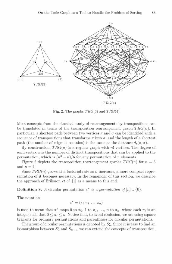
On the Toric Graph as a Tool to Handle the Problem of Sorting 83
123
213 231
312132
321
TRG(3)
1 2 3 4
1 2 4 3 1 3 2 4 1 3 4 2 1 4 2 3 2 1 3 4 2 3 1 4 2 3 4 1 3 1 2 4 3 4 1 2 4 1 2 3
4 3 2 1
3 4 2 14 2 3 12 4 3 13 2 4 14 3 1 24 1 3 21 4 3 24 2 1 32 1 4 33 2 1 4
3 1 4 22 4 1 3
TRG(4)
Fig. 2. The graphs TRG(3) and TRG(4)
Most concepts from the classical study of rearrangements by transpositions canbe translated in terms of the transposition rearrangement graph TRG(n). Inparticular, a shortest path between two vertices π and σ can be identified with asequence of transpositions that transforms π into σ, and the length of a shortestpath (the number of edges it contains) is the same as the distance dt(π, σ).
By construction, TRG(n) is a regular graph with n! vertices. The degree ofeach vertex π is the number of distinct transpositions that can be applied to thepermutation, which is (n3 − n)/6 for any permutation of n elements.
Figure 2 depicts the transposition rearrangement graphs TRG(n) for n = 3and n = 4.
Since TRG(n) grows at a factorial rate as n increases, a more compact repre-sentation of it becomes necessary. In the remainder of this section, we describethe approach of Eriksson et al. [1] as a means to this end.
Definition 8. A circular permutation πc is a permutation of [n] ∪ {0}.The notation
πc = (π0 π1 . . . πn)
is used to mean that πc maps 0 to π0, 1 to π1, . . ., n to πn, where each πi is aninteger such that 0 ≤ πi ≤ n. Notice that, to avoid confusion, we are using squarebrackets for ordinary permutations and parentheses for circular permutations.
The group of circular permutations is denoted by Scn. Since it is easy to find an
isomorphism between Scn and Sn+1, we can extend the concepts of transposition,

84 R. de A. Hausen et al.
transposition distance and sorting by transpositions to circular permutations.For instance, a transposition t(i, j, k), where 0 ≤ i < j < k ≤ n + 1, applied to
πc = (π0 π1 . . . πi−1 πi . . . πj−1 πj . . . πk−1 πk . . . πn)
yields
πct(i, j, k) = (π0 π1 . . . πi−1 πj . . . πk−1 πi . . . πj−1 πk . . . πn).
A permutation π = [π1π2 . . . πn] in Sn can be mapped to a circular permuta-tion in Sc
n by adding the element 0 before π1, producing the circular permutationπc = (0π1π2 . . . πn). Given a permutation π of n elements, the circularization ofπ is the circular permutation πc.
Definition 9. [1] Given a circular permutation πc = (π0 π1 . . . πj−1 πj . . . πn),a rotation of πc is a permutation of the form
πc t(0, j, n + 1) = (πj . . . πn π0 π1 . . . πj−1),
for some value 0 < j < n + 1.
We say that two circular permutations πc and σc are circularly equivalent, de-noted as πc ≡c σc, if σc = πc or if σc is a rotation of πc, that is πc t(0, j, n+1) =σc for some j (or, equivalently, σc t(0, j′, n + 1) = πc for some j′).
For instance, the following circular permutations are all circularly equivalent:(0 3 4 1 2) ≡c (3 4 1 2 0) ≡c (4 1 2 0 3) ≡c (1 2 0 3 4) ≡c (2 0 3 4 1).
Definition 10. [1] Let π be a permutation in Sn and m an integer. An m-stepcyclic value shift of π is the circular permutation
m + πc := (m m + π1 . . . m + πn),
where k is the remainder of the division of k by n + 1.
Example 1. Let π = [3 4 1 2]. The only circular permutations that result from acyclic value shift of π are:
1 + πc = (1 4 0 2 3) ≡c (0 2 3 1 4), 2 + πc = (2 0 1 3 4) ≡c (0 1 3 4 2),3 + πc = (3 1 2 4 0) ≡c (0 3 1 2 4), and 4 + πc = (4 2 3 0 1) ≡c (0 1 4 2 3).
Any cyclic value shift of the identity permutation [1 2 . . . n] generates a circularpermutation that is circularly equivalent to (0 1 2 . . . n). In a similar manner,a cyclic value shift of the reverse permutation [n n−1 . . . 1] yields a circularpermutation that is circularly equivalent to (0 n n−1 . . . 1).
Definition 11. [1] Two permutations π, σ are torically equivalent, π ≡◦◦ σ, ifπc ≡c m + σc for some integer m.

On the Toric Graph as a Tool to Handle the Problem of Sorting 85
From example 1, we can infer that [3 4 1 2], [2 3 1 4], [1 3 4 2], [3 1 2 4] and [1 4 2 3]belong to the same equivalence class under the toric equivalence relation. Weuse π◦◦ to denote the toric equivalence class of π.
As we can see in Theorem 2 and Corollary 1, it is possible to group verticesin TRG(n) according to their toric equivalence.
Theorem 2. [1] Let πσ be an edge of TRG(n). For every permutation π′ suchthat π′ ≡◦
◦ π, there is a permutation σ′ torically equivalent to σ such that π′σ′
is also an edge of TRG(n).
Corollary 1. [1] If two permutations π, π′ are torically equivalent, then dt(π) =dt(π′).
Definition 12. [1] The toric graph of order n, Tor(n) = (V, E), is a graphwhere each vertex in V corresponds to an equivalence class under the toric equiv-alence of the permutations of n elements, and the set of edges is:
E = {π◦◦σ
◦◦ |πσ is an edge of TRG(n)}.
The toric graphs Tor(3) and Tor(4) are depicted in Fig. 3.
[1 2 3]◦◦
[2 1 3]◦◦
[3 2 1]◦◦
[1 2 3 4]◦◦�� ��
[2 1 3 4]◦◦�
��
�
��
��
[3 4 1 2]◦◦�� ��
[2 4 1 3]◦◦ [3 1 4 2]◦◦�� ��[4 3 1 2]◦◦ [2 1 4 3]◦◦
�� ��[4 3 2 1]◦◦
Tor(3) Tor(4)
Fig. 3. The toric graphs Tor(3) and Tor(4)
3 New Results
We start this section with a connection between the classic approach using thereality and desire diagram and the less used approach by toric classes. After-wards, we characterize the toric equivalence classes that have only 1 element —the unitary classes — in the case n + 1 prime. This characterization is used tocalculate the size of the toric graph Tor(n). We also estimate the transpositiondistance between two unitary classes, an interesting result given the difficulty offinding bounds on the transposition distance.
Theorem 3. The reality and desire diagrams RD(π, ι) and RD(π′, ι) of twotorically equivalent permutations π, π′, respectively, are isomorphic graphs.

86 R. de A. Hausen et al.
Proof. Let π, π′ be two torically equivalent permutations. By the definition oftoric equivalence, there exists an integer m such that πc ≡c m +π′c. Comparingthe elements of πc and π′c, we have πi ≡ π′
i+�+ m (mod n + 1) for i = 0, . . . , n,
where � is such that π′� + m ≡ 0 (mod n + 1).
Let us now turn our attention to the reality and desire diagrams RD(π, ι) andRD(π′, ι). Both graphs are on the same set of vertices, and have the same setof desire edges
(+ i,−(i + 1)
), i = 0, . . . , n. In the remainder of this proof, we
will demonstrate that there is an isomorphism on that preserves the adjacencyof the vertices joined by reality edges.
In RD(π, ι), there exists a reality edge between +πi and −πj if, and only if,|πi − πj | = 1, where 0 ≤ i, j ≤ n. The equivalence
πi ≡ π′i+�
+ m (mod n + 1)
allows us to state that
|πi − πj | ≡∣∣∣π′
i+�+ m − (π′
j+�+ m)
∣∣∣ ≡
∣∣∣π′
i+�− π′
j+�
∣∣∣ (mod n + 1).
Therefore, a function Φ : V (RD(π, ι)) → V (RD(π′, ι)), such that Φ(±πi) =±π′
i+�, preserves adjacencies and is, consequently, an isomorphism. �
Theorem 3 can be used as an alternative proof for the fact that dt(π) = dt(π′)for two torically equivalent permutations π and π′ (Corollary 1).
Theorem 4. Let π be a permutation of n elements and π◦◦ its toric equivalenceclass. The number of elements in π◦
◦ divides n + 1.
Proof. By the definition of a cyclic value shift, (n + 1) + πc = πc. Let m′ be thesmallest positive integer such that m′+πc ≡c πc. The cyclic value shift km′+πc,where km′ is an integer multiple of m′, is circularly equivalent to πc, since that
km′ + πc ≡c m′ + . . . + m′︸ ︷︷ ︸
k
+πc ≡c m′ + . . . + m′︸ ︷︷ ︸
k−1
+(m′ + πc)
≡c m′ + . . . + m′︸ ︷︷ ︸
k−1
+πc ≡c . . .
≡c πc.
Suppose that m′ does not divide n+1; it means that n+1 = km′+r, for integersk, r, where 0 < r < m′. It follows that,
πc = (n + 1) + πc ≡c (r + km′) + πc = r + (km′ + πc) ≡c r + πc.
Or, more concisely, r +π ≡c π; but this equivalence contradicts the fact that m′
is the smallest positive integer such that m′ + π ≡c π. We conclude that m′ isindeed a divisor of n + 1. �
Corollary 2. If n+1 is prime, each toric equivalence class contains either 1 orn + 1 elements.

On the Toric Graph as a Tool to Handle the Problem of Sorting 87
In the case n + 1 is prime, it is also possible to characterize the classes thatcontain just 1 element. A toric equivalence class is said to be unitary if only 1element belongs to it. For instance, for n = 4 there are exactly 4 unitary classes,namely: [1234]◦◦ , [2413]◦◦ , [3142]◦◦ e [4321]◦◦.
Theorem 5. If n + 1 is prime, a toric equivalence class is unitary if, and onlyif, it is of the form [
k 2k 3k . . . �k . . . nk]◦◦ ,
where k is an integer, 1 ≤ k ≤ n.
Proof. For any integer k in the range 1 ≤ k ≤ n, if n + 1 is prime, then �k �≡0 (mod n + 1) for � = 1, . . . , n. We will show that a toric equivalence classthat contains the permutation [ k 2k 3k . . . nk ] is unitary. Consider thepermutation 1 + ( 0 k 2k 3k . . . nk ), and choose an integer �, 1 ≤ � ≤ n,such that �k + 1 = 0:
1 + ( 0 k 2k . . . nk ) == ( 0 + 1 k + 1 2k + 1 . . . �k + 1 (� + 1)k + 1 . . . nk + 1 )≡c (�k + 1 (� + 1)k + 1 . . . nk + 1 0 + 1 k + 1 2k + 1 . . . (� − 1)k + 1)= (0 �k + k + 1 . . . nk + 1 0 + 1 k + 1 2k + 1 . . . �k − k + 1)= (0 k 2k . . . nk).
By induction, m + (0 k 2k . . . nk) = 1 + . . . + 1︸ ︷︷ ︸m−1
+1 + (0 k 2k . . . nk) =
1 + . . . + 1︸ ︷︷ ︸m−1
+(0 k 2k . . . nk) = . . . = (0 k 2k . . . nk), so the toric equivalence
class of [k 2k . . . nk] is unitary.On the other hand, consider that π = [π1π2 . . . πn] is the only permutation
that belongs to a unitary class; this implies that m + πc is circularly equivalentto πc for any integer m, in particular for m = 1. That is,
(0π1π2 . . . πn) ≡c (1 π1 + 1 π2 + 1 . . . πn + 1).
Let � be such that π� + 1 = 0. So,
π�+1 + 1 = π1,π�+2 + 1 = π2,
...π�+n + 1 = πn,
that is, π�+i + 1 ≡ πi (mod n + 1) for every integer i between 1 and n. Sinceπi �= πj if i �= j, and 1 ≤ π1 ≤ n for every i between 1 e n, the system of modularequations is satisfiable if πi = ik where k = π�+1 + 1. �
Theorem 5 allows us to precisely determine the number of vertices of Tor(n),where n + 1 is prime. According to the theorem, if n + 1 is prime, there are

88 R. de A. Hausen et al.
exactly n unitary toric equivalence classes. It follows that the remaining n! − nvertices of TRG(n) are distributed among classes of size n+1, that is, there areexactly n!−n
n+1 classes of size n + 1. Theorem 6 summarizes this result.
Theorem 6. If n + 1 is prime, Tor(n) has exactly n!−nn+1 + n vertices.
We will now adopt a more compact representation for the unitary classes, inthe form of Un,k, meaning the unitary toric equivalence class that contains thepermutation of n elements that starts with the element k, that is,
Un,k :=[
k 2k 3k . . . �k . . . nk]◦◦ .
Theorem 7. Let π be a permutation that belongs to a unitary class Un,k, wheren + 1 is prime and k > 1. Then RD(π, ι) has only one cycle.
Proof. Let C = 0,−π1, +π1 − 1, . . . ,−1, 0 be the cycle in RD(π, ι), starting fromvertex 0 and following the reality edge incident to it. Given a vertex +i in thediagram, let s(+i) be the first successor of +i in cycle C, according to the order,that is non-negative, i. e., s(+i) appears in C after following a reality edge andsubsequently a desire edge. For instance, s(0) = +π1 − 1 in every diagram, andin Fig. 1, s(0) = +2, s(+2) = +4, s(+4) = +6, s(+6) = +1, s(+1) = +3,s(+3) = +5, s(+5) = 0.
Since π belongs to a unitary class, we know that π1 = k — note that, as a con-sequence, we have s(0) = +π1 − 1 = +k − 1 — and we can write any element π�
as �k, so the sequence {0, s(0), s(s(0)), . . .} is equal to {0, +�1k, +�2k, . . . , +�xk},for integers �1, �2, . . . , �x (where x, for now, is unknown). This means that
s(0) = +�1k.
Since s(0) is also equal to +k − 1, we have the identity
+ �1k = +k − 1. (1)
Generalizing the above identity, we have
s(+�pk) = +�p+1k,
and also s(+�pk) = +(�p + 1)k − 1, which gives us
+ �p+1k = +(�p + 1)k − 1. (2)
We summarize identities 1 and 2 in the following recurrence relation:{
�1k ≡ k − 1 (mod n + 1)�pk ≡ �pk + k − 1, for p > 1,
which has the following equivalence as a solution
�pk ≡ (p + 1)(k − 1) (mod n + 1).

On the Toric Graph as a Tool to Handle the Problem of Sorting 89
Hence the sequence {0, +�1k, +�2k, . . . , +�xk} becomes
{0, +k − 1, +2(k − 1), . . . , +x(k − 1)}.
As we must have that s(+x(k − 1)) = 0, the only value of x that satisfies theequation (x + 1)(k − 1) = 0 is x = n. That is, the sequence contains everyelement of π and, consequently, there is only one cycle in RD(π, ι).
As a byproduct of our proof, we immediately notice that the sequence of suc-cessive elements {+k − 1, +2(k − 1), . . . , +n(k − 1)} in the cycle corresponds tothe same sequence of elements {σ1, σ2, . . . , σn} in a permutation σ that belongsto the unitary class Un,k−1. �
Corollary 3. If n + 1 is prime, a permutation π �= ι that belongs to a unitaryclass satisfies dt(π, ι) ≥ n/2.
Corollary 3 hints us there is some symmetry in the toric graph when n + 1 isprime. It also tells us that the transposition distance from the identity to theunitary classes is close to the known bounds for the transposition diameter [1,2],which indicates they are good samples for studying the behavior of Dt(n).
4 Conclusion
Corollary 3 is an interesting development of the approach advocated in this pa-per. We have found the lower bound dt(π, σ) ≥ n/2 is very close to the exacttransposition distance between the two permutations π, σ belonging to two dif-ferent unitary classes, never differing by more than 1 transposition, as it can beseen in Table 1. We have used a Dias’ implementation [7] of a branch-and-boundalgorithm, modified to take advantage of the equivalence classes, to exactly de-termine the transposition distance of the unitary classes dt(Un,k, ι), for valuesof n up to 18 such that n + 1 is prime. In a future paper, we hope to formallydemonstrate Conjecture 1 — related to Meidanis, Walter and Dias’ [2] result forthe reverse permutation.
Conjecture 1. If n + 1 is prime and π belongs to a unitary class Un,k, thenn/2 ≤ d(π) ≤ n/2 + 1.
Table 1. Transposition distances dt(Un,k, ι) and the diameter Dt(n)
dt(Un,k, ι)k
Dt(n)2 3 4 5 6 7 8 9 10 11 12 13 14 15 16 17 18
n
4 2 2 3 — — — — — — — — — — — — — — 36 3 4 3 4 4 — — — — — — — — — — — — 4
10 5 6 6 6 5 6 6 6 6 — — — — — — — — 612 6 7 7 7 6 6 7 7 7 6 7 — — — — — — 716 8 9 8 9 9 9 8 8 9 9 9 8 9 8 9 — — 9 or 1018 9 9 10 10 10 10 9 10 9 10 9 9 9 9 10 10 10 10 or 11

90 R. de A. Hausen et al.
We have noted by looking at the reality and desire diagram that the most dis-tant permutations, with respect to the identity, always have either 0, 1 or 2 oddcycles in every example we could conceive. For 3 ≤ n ≤ 12 and n = 14, the di-ameter is attained by the reverse permutation, which always has less than 3 oddcycles. For n = 13 and n = 15, the most distant permutations found by Erikssonet al. [1] have 2 odd cycles. For n odd, n > 15, Elias and Hartman [5] describedpermutations that are more distant to the identity than the reverse permuta-tion — requiring more than �n/2�+1 transpositions — and those permutationshave also 2 odd cycles. We hope that the combined use of the reality and desirediagram and the toric graph may provide an answer as to why this happens.For even values of n where n + 1 is prime, the permutations having the smallestnumber of odd cycles are those that have 1 odd cycle, and we believe those per-mutations are good candidates to investigate the transposition diameter Dt(n),as it can be seen in the following conjecture.
Conjecture 2. Let Ω be the set of permutations with just one odd cycle in thereality and desire diagram, and Δ be the set of permutations whose transpositiondistance is equal to Dt(n). If n + 1 is prime, then Ω ∩ Δ �= ∅.Another interesting result that seems to be close to achievement is the determi-nation of the transposition diameter Dt(16). All the values of Dt(n), for n < 16have been exactly determined but, to this day, Dt(16) is still undetermined, ly-ing within 9 ≤ Dt(16) ≤ 10. Notice that 16 + 1 is prime, so it is one of thecases where more information can be derived from the toric graph, as shown inSect. 3 of this paper. Given the symmetry of the toric graph for n + 1 prime, wehope that Dt(16) is equal to the distance dt(π, ι) for some π in a unitary class.If this scenario turns out to be true, then Dt(16) would be 9. Actually, a bolderconjecture is: for even n such that n + 1 is prime, Dt(n) = n/2 + 1, a resultthat would determine an infinite family of even values of n for which Meidanis,Walter and Dias’ conjecture [2] holds.
Acknowledgment. The authors wish to thank Andre Korenchendler (UFRJ)for modifying Dias’ implementation to speed-up the process of finding the trans-position distances.
References
1. Eriksson, H., Eriksson, K., Karlander, J., Svensson, L., Wastlund, J.: Sorting abridge hand. Discrete Math. 241(1), 289–300 (2001)
2. Meidanis, J., Walter, M.E.M.T., Dias, Z.: Transposition distance between a per-mutation and its reverse. In: Baeza-Yates, R. (ed.) Proceedings of the 4th SouthAmerican Workshop on String Processing, Valparaıso, Chile, pp. 70–79. CarletonUniversity Press (1997)
3. Setubal, C., Meidanis, J.: Introduction to Computational Molecular Biology. PWSPublishing (January 1997)

On the Toric Graph as a Tool to Handle the Problem of Sorting 91
4. Bafna, V., Pevzner, P.A.: Sorting by transpositions. SIAM J. Discrete Math. 11(2),224–240 (1998)
5. Elias, I., Hartman, T.: A 1.375-approximation algorithm for sorting by transposi-tions. IEEE/ACM T. Comput. Bi. 3(4), 369–379 (2006)
6. Bafna, V., Pevzner, P.A.: Genome rearrangements and sorting by reversals. SIAMJ. Comput. 25(2), 272–289 (1996)
7. Dias, Z.: Rearranjo de genomas: uma coletanea de artigos. PhD thesis, Unicamp,Campinas, Sao Paulo (2002)

A Customized Class of Functions for
Modeling and Clustering Gene ExpressionProfiles in Embryonic Stem Cells
Shenggang Li1, Miguel Andrade-Navarro2, and David Sankoff1
1 Department of Mathematics and Statistics, University of Ottawa, Canada2 Max Delbruck Center for Molecular Medicine, Berlin-Buch, Germany
Abstract. Based on the trajectories of individual genes, we address theproblem of clustering time course gene expression data for embryonicstem cells (ESC) differentiation. We propose a class of functions deter-mined by only two parameters but flexible enough to model realistic timecourses. This serves as a basis for a mixed model clustering method. Thismethod takes into account (1) genetic function profile induced or con-trolled by other regulators, (2) unobservable random effects producingheterogeneity within gene clusters, and (3) autoregressive componentsdefining the stochastic and autocorrelation structures. We employ anEM algorithm to fit the mixture model and clustering follows monitoringvia Bayesian posterior probabilities. Our method is applied to a mouseESC line during the first 24 hours of differentiation period. We assess thebiological credibility of the results by detecting significantly associatedFatiGO Gene Ontology terms for each cluster.
1 Introduction
Cluster analysis of gene expression profiles over a time course often treat eachsampling time as one of the dimensions of a multivariate variable, reducingthe problem of clustering the gene trajectories to one of clustering multivariateobservations. Since the object of gene expression clustering is to detect commontrajectories, however, this “static” multivariate characterization loses power andprecision, since the temporal order plays no role in the analysis; indeed the timescan be permuted in any order without changing the results of the cluster analysis.
Gene expression profiles during cell growth, differentation, tissue activationof various kinds, and during cyclical changes tend to follow well-defined pat-terns and are often highly autocorrelated. These facts lead to the incorporationof more “dynamic” considerations into clustering procedures. Model-based clus-tering techniques [9] incorporate dynamical features by implementing formalstatistical modeling and parametric models in preference to pure data mining.
A number of model-based clustering methods for dynamical gene expressiondata have been proposed [1,5,14,17]. Here a group of genes following the sameprobability model fall into the same cluster, taking into account autoregres-sive and other random effects. For example, [19] discusses autoregressive modelsfor clustering time course gene expression data. [2,11] apply cubic spline andB-spline mixture models to analyze gene expression time series data.
A.L.C. Bazzan, M. Craven, and N.F. Martins (Eds.): BSB 2008, LNBI 5167, pp. 92–103, 2008.c© Springer-Verlag Berlin Heidelberg 2008

A Customized Class of Functions for Modeling and Clustering 93
Purely autoregressive models, however, only consider autocorrelative structurewithout explicitly taking account of other properties of functional interactionsamong genes. Although a p-order autoregressive model may explain a p-orderpolynomial time trend effect, it fails to match exponential time growth effectssuch as exp(λt) or periodic effects such as sin(ωt). Spline techniques can representdata trends but still remain essentially black boxes [8] with respect to geneticfunctions. [8] suggests a novel clustering technique based on gene functionalcurves, making use of plausible biological models for gene expression dynamics.
1.1 The Proposed Model
Here we treat a gene profile over a time course as composed of the followingcomponents
1. impact of related genes or other regulation mechanisms (modeled as a dy-namical system of differential equations),
2. autoregressive factors representing autocorrelation structure and feedbackor loop effects,
3. random components allowing for heterogeneity among the individual genesin each cluster.
This method is flexible in assigning both dynamic and fixed functional com-ponents into an integrated time series model with random mixtures. We notethat by appropriately incorporating randomness into the model we can avoidthe tendency to generate clusters based purely on chance properties of the data.
2 The Mixture Time Series Model for Functional CurveClustering
We denote an expression profile (or observation vector over time course) of anindividual gene gi as Yi = (yi1, yi2, . . . . , yiT ). In this notation T refers to the totalnumber of time points sampled over a time course. Our objective is to clustertarget genes into distinct clusters in terms of the similarities of gene functionalbehavior. Genes are grouped together on the basis of the form of their expressionprofiles (curve shapes) rather than similarity in Euclidean distance. The model-based clustering analysis assumes that the genes in every cluster will perfectly fitan underlying mixture time series model, whereany gene profile Yi is consideredas an observation of a functional curve following the probability model:
Yit = Gene Network Interactions + Auto Effects+ Time−dependent Random Effect + Noise (1)
If all target genes gi, i = 1, 2, . . . , N satisfy the model above, then the Yit, i =1, 2 . . . , N are generated by the following model:
Yit = f (c)(t|Φ(c))+t−1∑
j=t−p
αjcYij+γc+ε (t = 1, 2 . . . , T and i = 1, 2, . . . , N), (2)

94 S. Li, M. Andrade-Navarro, and D. Sankoff
where the “within” random effect γc ∼ normal(0,τ2c ) (c = 1, 2, . . . , C) are
independent of each other, indicating that genes in the same cluster have aunified correlation structure, ε is the i.i.d. white noise ∼ normal(0,σ2), the trendcurve f (c)(t|Φ(c)) contains the internal function effect of gi, combined with theother network interactions (or regulatory effect on gi), and Φ(c) is the parameterset for the fixed mean curve in cluster c (c = 1, 2, . . . , C). We have includedautoregressive items in the model because we wish to capture feedback or loopeffects in genetic pathways.
The key problem here is to determine the form of function f (c)(t|Φ(c)). Wewill estimate it with the trend deduced from a genetic transcription model. TheB spline techniques previously employed to deal with this problem [11] have nodirect biological functional interpretation. Instead we are inspired Chen’s lineartranscription model [7] to elaborate a function f (c)(t|Φ(c)). Chen’s model is anonlinear dynamic system with the following form:
drdt = Cp − V r dp
dt = Lr − Up (3)
where r is the mRNA concentration, p is the protein concentration, L containsthe translational constants, V is the degradation rate of mRNA and U is thedegradation rate of proteins. According to Theorem 1 in [7], the solution tomodel (3) has form:
x(t) = Q(t)etλ (4)
where Q(t) = {qij} is a 2n × 2n matrix whose elements are polynomial func-tions of t. In [7] it is stated that a gene system should be stable system and itsexpression should not have an exponential or a polynomial growth rate, whichimplies that Q(t) is a constant and x(t) is actually an ordinary exponential func-tion. However, an exponential function is monotonic and cannot fully reflect thewave-like shapes that characterize many gene functional curves. Consequentlywe do not adopt (4) directly, though we will utilize features of (3) and (4) todevelop a more effective functional curve.
To do so so, we have studied the functional gene curves of mouse embryonicstem cells (mESC) in the first 24 hours of differentiation (for experimental detailsand the data bank, see [10]) and found that gene expression of these genes canbe well described by the following hyperbolic function:
f(t) =1
exp[b(t − a) +√
1 + (t − a)2](5)
To see the connection between (5) on one hand and (3) and (4) on the other, wenote that the gene’s growth rate satisfies:
df(t)dt
= −[b +t − a√
1 + (t − a)2]f(t), (6)
where the expression (6) indicates that this gene system also remains stable,but is more flexible than the one in (3). Here t−a√
1+(t−a)2is restricted to the
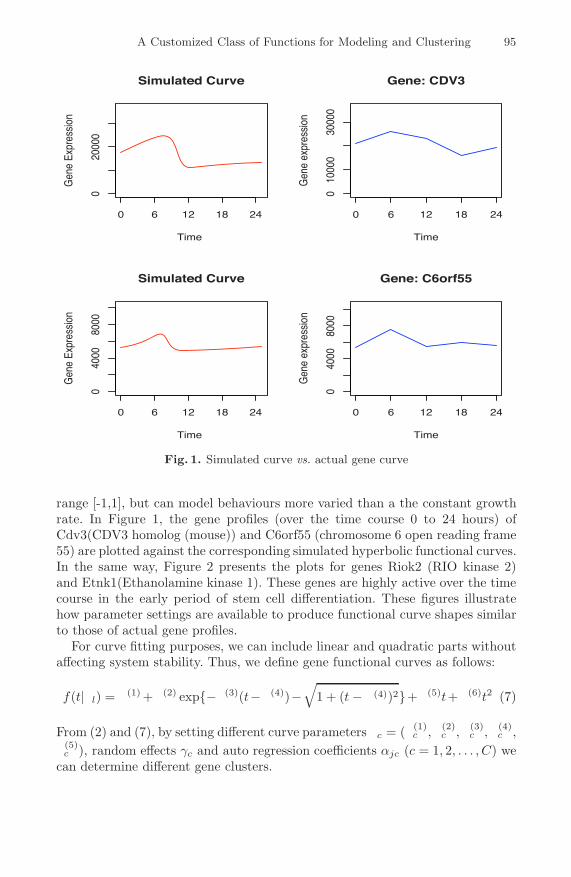
A Customized Class of Functions for Modeling and Clustering 95
Simulated Curve
Time
Gen
e Ex
pres
sion
0 6 12 18 24
020
000
Gene: CDV3
Time
Gen
e ex
pres
sion
0 6 12 18 24
010
000
3000
0
Simulated Curve
Time
Gen
e Ex
pres
sion
0 6 12 18 24
040
0080
00
Gene: C6orf55
Time
Gen
e ex
pres
sion
0 6 12 18 24
040
0080
00
Fig. 1. Simulated curve vs. actual gene curve
range [-1,1], but can model behaviours more varied than a the constant growthrate. In Figure 1, the gene profiles (over the time course 0 to 24 hours) ofCdv3(CDV3 homolog (mouse)) and C6orf55 (chromosome 6 open reading frame55) are plotted against the corresponding simulated hyperbolic functional curves.In the same way, Figure 2 presents the plots for genes Riok2 (RIO kinase 2)and Etnk1(Ethanolamine kinase 1). These genes are highly active over the timecourse in the early period of stem cell differentiation. These figures illustratehow parameter settings are available to produce functional curve shapes similarto those of actual gene profiles.
For curve fitting purposes, we can include linear and quadratic parts withoutaffecting system stability. Thus, we define gene functional curves as follows:
f(t|βl) = β(1) +β(2) exp{−β(3)(t−β(4))−√
1 + (t − β(4))2}+β(5)t+β(6)t2 (7)
From (2) and (7), by setting different curve parameters βc = (β(1)c , β
(2)c , β
(3)c , β
(4)c ,
β(5)c ), random effects γc and auto regression coefficients αjc (c = 1, 2, . . . , C) we
can determine different gene clusters.

96 S. Li, M. Andrade-Navarro, and D. Sankoff
Simulated Curve
Time
Gen
e Ex
pres
sion
0 6 12 18 24
010
0030
00
Gene: Riok2
Time
Gen
e ex
pres
sion
0 6 12 18 24
020
0040
00
Simulated Curve
Time
Gen
e Ex
pres
sion
0 6 12 18 24
040
0080
00
Gene: Etnk1
Time
Gen
e ex
pres
sion
0 6 12 18 24
040
0080
00
Fig. 2. Simulated curve vs. actual gene curve
To implement cluster recognition, we assume the following mixture-densitymodel:
P (Y |Θ, Ω) =C∑
c=1
ωcpc(Y |θc), (8)
where the parameter set Θ = (β1, . . . , βC , αj1, . . . , αjC , γ1, . . . , γC) (j=1,2. . . ,p)and Ω = (ω1, . . . , ωC) such that
∑Cc=1 ωc = 1 and pc(Y |θc) is the density function
generated by the model (2) defined previously. Given observed samples Y =(Y1, Y2, . . . , YN ), the log-likelihood expression for the above mixture density is:
log(P (Y |Θ, Ω)) = log(C∑
c=1
ωcpc(Y |θc)) =N∑
i=1
log(C∑
c=1
ωcpc(Yi|θc)), (9)
where Yi = (yi1, yi2, . . . . , yiT ) (i = 1, 2, . . . , N) represents the profile of gene gi
over the time course t = 1, 2, . . . , T . Since it is hard to optimize (9) by ordinaryanalytical methods, we will apply the well known expectation maximization(EM)algorithm [13] to estimate these parameters. The details of the EM algorithmapproach and the corresponding inference technique is given in the Appendix.

A Customized Class of Functions for Modeling and Clustering 97
3 Numerical Tests
3.1 Clustering Results
In this section we illustrate the result of clustering gene profiles for V6.5 mouseembryonic stem cells over the time course [0h, 6h, 12h, 18h, 24h],which representsthe early period of mESC differentiation. At the first stage, we select as targetgenes 419 with high differential expression as detected by the SAM method [18].A standardization procedure is first applied to all gene profiles before runningthe clustering program. We arbitrarily choose a small number of clusters, namelyC = 3, in order to facilitate the evaluation of the method, and set the initialcluster proportion to be 1
3 . Thus, we will optimize (9) with respect to Θ =(θ1, θ2, θ3) , Ω = (ω1, ω2, ω3) and σ2.
Figure 3 presents the results of clustering the 419 genes. The three clustersclearly have different patterns over the time course. Briefly, cluster one is basi-cally up-regulated compared to cluster three which has a distinct down-regulatedpattern. Cluster two contains the largest number of genes. Note that that theseclusters have different “compactness” levels. For instance, cluster three is char-acterized by the fact that the gene functional curves are more closely intertwinedwhile cluster two is more loosely arranged, indicating a larger intra-cluster varia-tion. This effect is captured by the different random gene effect within the threeclusters, a feature of the mixture model. In visually assessing the clusters, wemust recall that the curves are not clustered by the overall proximity to eachother, but by the similarities of their patterns.
We choose the order of autoregressive component to be 1 (i.e. p = 1) to avoidthe increased noise effect associated with larger order components demonstratedin numerical experiments [11].
To validate the clustering, we characterized the genes in each cluster by com-piling Gene Ontology (GO) terms. We also searched the FatiGO server to com-pare the three clusters. Table 1 displays the distribution of genes featured bydifferent biological processes.
Table 1. Distribution (%) of genes according to biological process
Biological Functions Cluster one Cluster two Cluster three
RNA metabolic 17.14 40.57 42.65Cellular lipid metabolic 13.33 2.83 1.47
Cellular protein metabolic 45.71 29.25 35.29Nucleoside, nucleic metabolic metabolic 25.64 50.91 52.94
Regulation of cellular process 23.29 43.64 27.42Cellular macromolecule metabolic 43.84 28.18 35.59
Protein metabolic 43.84 30.02 38.24Transcription 18.57 33.33 20.97
Cellular biosynthetic process 21.92 13.76 27.42Biosynthetic process 24.66 14.16 28.97
N 94 153 85

98 S. Li, M. Andrade-Navarro, and D. Sankoff
1 2 3 4 5 6
−3
−1
12
3
Cluster One
Time Unit
Ge
ne
exp
ress
ion
1 2 3 4 5 6
−3
−1
12
3
Cluster two
Time Unit
Ge
ne
exp
ress
ion
1 2 3 4 5 6
−3
−1
12
3
Cluster three
Time Unit
Ge
ne
exp
ress
ion
Fig. 3. Clustering result for gene profiles of V6.5 embryonic stem cells
3.2 Biological Analysis
Cluster one includes 119 genes, of which 94 had associated GO terms, largelywith protein metabolism, processing of macromolecules and catalytic functions,such as Sc4mol, the Rpl and Rps family (Rpl4 Rpl13 Rpl14 Rpl23 Rpl41 Rps2Rps6 Rps12 Rps17 Rpl22 Rps27 Rps28 Rps27l), Uba52, Csnk1e, Otx2, Igfbp2and Gpi1. These genes follow a generally up-regulated trend during ESC differ-entiation and participate in ESC metabolism or protein synthesis processes. Forexample, Otx2 is an early stage murine ESC marker playing a cental role in gas-trulation, essential for the early specification of the neuroectoderm destined tobecome fore midbrain [15]. Csnk1e, which undergoes a persistent up-regulationpattern over the time course, performs a catalytic function for serine/threoninekinase activity. The Rpl/Rps family is involved in ribosomal structure and henceprotein biosynthesis. Note that there was some evidence, discounted by the au-thors as well as our results here, that Rpl4 and Rps24 are among the genesconstituting a unique molecular signature in human ESC [3].

A Customized Class of Functions for Modeling and Clustering 99
There are 198 genes in cluster two, 153 with GO annotations. These genes areinvolved in RNA metabolism, regulation of cellular process and DNA-dependenttranscription. Many key ESC markers such as Nanog, Sox21, Zfp57, Cbx7, Vcl,Dnajb6, Msi2h and Cggbp1 fall into this cluster. They generally usually down-regulated for the first 18 or 24 hours and are up-regulated later. By checking thecorrelation distance, we found these gene profiles are remarkably similar to theexpression patterns of undifferentiated ESC markers such as OCT4, Sox2 andFoxd3. From the point of view of stem cell differentiation, these genes are crucialfor stem cell self-renewal and maintenance of the inner cell mass (ICM) of theblastocyst. With the loss of cell proliferation and pluripotency, they undergo asignificant and persistent down-regulation pattern [6,16].
Many members of cluster two are also related to the cell cycle, cell prolifer-ation or growth. For example, C2ORF29, Cdv3 and Rbbp7 are involved in cellproliferation. Socs3 and Ltbp4 function in the regulation of cell growth. Nmyc1,Cdk2ap1, Nipbl, Cdc34, Mcm5, Nipbl, BC068171 and Ccne1 are cell-cycle re-lated genes. They mediate the progression through the cell cycle, particularlythe G1/S transition of the mitotic cell. That these genes are in cluster two agreeswith theories [12], whereby the cells initially derived from a population of stemcells undergo rapid cell division during early differentiation; throughout this pe-riod, expression of genes keeping control of the cell cycle or proliferation shouldbe attenuated.
Another 102 genes are found in cluster three, 85 with GO annotations. Com-pared with cluster one, cluster three is enriched for genes in charge of nucle-obase, nucleoside, nucleotide and nucleic acid metabolic process, such as Ctbp2,Cdk2ap1, Apex1, Hmgb2, Mybbp1a Ran, Gars, H2afz, Sod2, Nola2, Mki67ip,Etv4, Atp5l, Bzw1, Nr0b1, Klf5, Rbm14, Polr2f, Ankrd17, Lsm3, Zfp36l1, Ddx5,Sfrs1, Rbm3, Cars and Psmc5. This cluster is also associated with microtubule-based movement, signal transduction and biosynthetic processes. These includeArpc4, Lefty1, Ptprf, Stmn1, Cfl1, Trh and Eif4ebp1. Lefty1 is an important“stemness” marker expressed in the left half of gastrulating mouse embryos andinvolved in the TGF-beta signaling pathway. Ptprf has an intrinsic protein ty-rosine phosphatase activity (PTPase) and plays a role in cell adhesion receptorand the insulin signaling pathway. Ptprf has also been identified in human ESCstudies. Stmn1 is involved in signal transducing, participates in the regulation ofthe microtubule (MT) filament and promotes disassembly of microtubules. Trhplays a role in cell-cell signaling and neuroactive ligand-receptor interaction.Arpc4 is related to cytoskeleton and actin filament polymerization.
Since clusters two and three have a similar down-regulated pattern, especiallyin the first 12 hour period, it is not surprising that some of their members havesimilar gene functions in signalling, ATP/GTP binding, actin binding and micro-tubules. For example, the genes Pfn1, Wdr1, Efna2, Lefty2, Ak7, Ptch1, Riok2,Arf6 and Actg1 are classified into cluster two. This is not surprising; mainte-nance of the pluripotent state of ESC requires intrinsic signalling as well asextrinsic environmental elements, involving microtubules. It is known that envi-ronmental factors such as cell-surface receptors and cytokines play an important

100 S. Li, M. Andrade-Navarro, and D. Sankoff
Table 2. Over-represented GO terms for each cluster from GOstat
Cluster Biological Function In cluster In genome P-value
I primary metabolic process 60 5694 0.000107cellular protein metabolic process 34 2421 7.44E-05structural constituent of ribosome 14 147 4.41E-10
Total 94 14456
II gene expression 57 2452 4.21E-08RNA metabolic process 46 2082 1.59E-05transcription, DNA-dependent 35 1704 0.00215ribonucleoprotein complex biogenesis 11 174 0.000302translational initiation 5 40 0.00266glycolysis 5 42 0.00326
Total 153 14456
III gene expression 33 2452 2.02E-05translation 13 369 2.50E-05amino acid,derivative metabolic process 9 264 0.00111ribonucleoprotein complex 10 382 0.00267
Total 85 14456
role in the maintenance of stem cell functions [12]. Transcription profiles of thistype generally take a persistent down-regulated pattern during differentiation.Examples include the actin binding related gene Ptprf and receptor activity-associated gene Tagln, which decrease sharply throughout the first 24 hours inESC differentiation.
Table 2 uses a t-test to evaluate the over-representation of various kinds ofGO terms in each cluster. The analysis in Table 2 confirms and deepens that ofTable 1. For example, the high value for RNA metabolism in cluster 2 possiblyresults from the selection of genes involved in transcriptional regulation. Thehigher proportion of cellular protein metabolic process in cluster 1, amino acidderivative metabolic processes and ribonucleoprotein complex, in cluster 3, areall closely related to protein biosynthesis. This similarity possibly originatesfrom genes involved in translation process(cluster 3). We also found interestingto see five glycolitic enzymes in cluster 2, and a number of genes involved in theformation of RNA-protein complexes in clusters 2 and 3. In the case of cluster2, this includes five genes involved in translation initiation.
References
1. Aach, J., Church, G.M.: Aligning gene expression time series with time warpingalgorithms. Bioinformatics 17, 495–508 (2001)
2. Bar-Joseph, Z., Gerber, G., Gifford, D., Jaakkola, T., Simon, I.: Continuous rep-resentations of time-series gene expression data. Journal of Computational Biol-ogy 10, 341–356 (2003)

A Customized Class of Functions for Modeling and Clustering 101
3. Bhattacharya, B., Miura, T., Brandenberger, R., Mejido, J., Luo, Y., Yang, A.X.,Joshi, B.H., Ginis, I., Thies, R.S., Amit, M., Lyons, I., Condie, B.G., Itskovitz-Eldor, J., Rao, M.S., Puri, R.K.: Gene expression in human embryonic stem celllines: unique molecular signature. Blood 103, 2956–2964 (2004)
4. Bilmes, J.A.: A Gentle Tutorial of the EM Algorithm and its Application to Pa-rameter Estimation for Gaussian Mixture and Hidden Markov Models. TechnicalReport 97-021. International Computer Science Institute, Berkeley, CA (1997)
5. Brumback, B.A., Rice, J.: Smoothing spline models for the analysis of nested andcrossed samples of curves. Journal of the American Statististical Association 93,961–976 (1998)
6. Chambers, I., Colby, D., Robertson, M., Nichols, J., Lee, S., Tweedie, S., Smith,A.: Functional expression cloning of Nanog, a pluripotency sustaining factor inembryonic stem cells. Cell 113, 643–655 (2003)
7. Chen, T., He, H.L., Church, G.M.: Modeling gene expression with differential equa-tions. In: Pacific Symposium on Biocomputing, pp. 29–40 (1999)
8. Chudova, D., Hart, C., Mjolsness, E., Smyth, P.: Gene expression clustering withfunctional mixture models. In: Advances in Neural Information Processing, vol. 16.MIT Press, Cambridge (2004)
9. Fraley, C., Raftery, A.E.: How many clusters? Which clustering method? Answersvia model-based cluster analysis. Computer Journal 41, 578–588 (1998)
10. Hailesellasse Sene, K., Porter, C.J., Palidwor, G., Perez- Iratxeta, C., Muro, E.M.,Campbell, P.A., Rudnicki, M.A., Andrade-Navarro, M.A.: Gene function in mouseembryonic stem cell differentiation. BMC Genomics 8, 85 (2007)
11. Luan, Y., Li, H.: Clustering of time-course gene expression data using a mixed-effects model with B-splines. Bioinformatics 19, 474–482 (2003)
12. Martinez Arias, A., Stewart, A.: Molecular Principles of Animal Development.Oxford University Press, NY (2002)
13. McLachlan, G.J., Krishnan, T.: The EM Algorithm and Extensions. John Wileyand Sons, New York (1997)
14. Medvedovic, M., Yeung, K.Y., Bumgarner, R.E.: Bayesian mixture model basedclustering of replicated microarray data. Bioinformatics 20, 1222–1232 (2004)
15. Morsli, H., Tuorto, F., Choo, D., Postiglione, M.P., Simeone, A., Wu, D.K.: Otx1and Otx2 activities are required for the normal development of the mouse innerear. Development 126, 2335–2343 (1999)
16. Niwa, H., Burdon, T., Chambers, I., Smith, A.: Self-renewal of pluripotent embry-onic stem cells is mediated via activation of STAT3. Genes and Development 12,2048–2060 (1998)
17. Ramoni, M.F., Sebastiani, P., Kohane, I.S.: Cluster analysis of gene expressiondynamics. Proceedings of the National Academy of Sciences USA 99, 9121–9126(2002)
18. Tusher, V.G., Tibshirani, R., Chu, G.: Significance analysis of microarrays appliedto the ionizing radiation response. Proceedings of the National Academy of SciencesUSA 98, 5116–5121 (2001)
19. Wu, F., Zhang, W.J., Kusalik, A.J.: Dynamic model-based clustering for time-course gene expression data. Journal of Bioinformatics and Computational Biol-ogy 3, 821–836 (2005)

102 S. Li, M. Andrade-Navarro, and D. Sankoff
A Appendix: EM Algorithm of Mixture Model
A.1 Inference of the Log-Likelihood Function for the MixtureModel
For convenience,we only consider the first order autoregressive item (i.e. p = 1in model (2)). According to model (2), we infer that if the gene gi belongs tocluster c then its expression profile Yi = (yi1, . . . , yiT ) at time point t satisfiesthe following conditional probability model:
P (yit|θc, Yi(t−1))) = Normal(f (c)(t|Φ(c)) + αcyi(t−1)), γc2 + ε2) (10)
Thus, the log-likelihood for Yi over time course t = 1, 2, . . . , T is
Lc(Yi|θc) = log[P (yi1|θc)T∏
j=2
P (yij |θc, yi(j−1))] (11)
From expression (10), (11) can be finally expressed as
Lc(Yi|θc) = C0−TLog(σi)− 1
2σi[(yi1−f(1|βc)−μ0)
2+TX
j=2
(yij−f(j|βc)−α(c)yi(j−1))2]
(12)
where the variance of Yi, σi =√
γ2c + ε2, C0 is a constant and μ0 represents the
mean at the initial time point. The log-likelihood of the mixture model of totalobserved samples can be expressed as
L(Y |Θ, Ω) =N∑
i=1
log(C∑
j=1
ωjPj(Yi|θj)) (13)
where Pj(Yi|θj) is identified by exp(Lj(Yi|θj)), and ωj, (j = 1, . . . , C) are theunknown cluster membership parameters such that
∑Cj=1 ωj = 1.
A.2 EM Algorithm Approach
The optimization for (12) can be carried out by using an EM algorithm. To seethe specific computational steps, the reader can refer to [4].
1. Set initial parameters Θ(0) = (θ(0)1 , . . . , θ
(0)C ) for the given number of clusters
C and cluster proportion Ω(0) = (ω(0)1 , . . . , ω
(0)C ).
2. Define cluster membership (a random variable) l, where l ∈ {1, 2, . . . , C} andl = c if gene gi belongs to cluster c. For k = 0, 1, 2, . . . repeat the followingiterative steps until a given threshold is reached.
3. E-step: Calculate the posterior of the cluster membership l given Yi, Θ(k)
and Ω(k) at the kth iterative step from the following procedure:
P (l|Yi, Θ(k), Ω(k)) =
ω(k)l Pl(Yi|θ(k)
l )∑C
j=1 ω(k)j Pj(Yi|θ(k)
j )(14)

A Customized Class of Functions for Modeling and Clustering 103
4. M-step: Maximize the expected posterior log-likelihood with respect to clus-ter membership parameters Ω and model parameters Θ given observed Yand current parameter estimates:
ω(k+1)l =
1N
N∑
i=1
P (l|Yi, Θ(k), Ω(k)) (15)
and
Maximize F =C∑
l=1
N∑
i=1
[Ll(Yi|θ(k+1)l )P (l|Yi, Θ
(k), Ω(k))] (16)
where (16) can be maximized by non-linear optimization techniques such asBFGS or the conjugate gradients method. Note that solving (16) is mucheasier than directly optimizing (9).

A.L.C. Bazzan, M. Craven, and N.F. Martins (Eds.): BSB 2008, LNBI 5167, pp. 104–114, 2008. © Springer-Verlag Berlin Heidelberg 2008
Extracting Information from Flexible Receptor-Flexible Ligand Docking Experiments
Karina S. Machado, Evelyn K. Schroeder, Duncan D. Ruiz, Ana Wink, and Osmar Norberto de Souza
Laboratório de Bioinformática, Modelagem e Simulação de Biossistemas – LABIO Programa de Pós-Graduação em Ciência da Computação, Faculdade de Informática,
PUCRS, Av. Ipiranga, 6681 – Prédio 32, sala 602, 90619-900, Porto Alegre, RS, Brazil {karina.machado,duncan.ruiz,ana.wink,osmar,norberto}@pucrs.br
Abstract. Recent progress in structural biology and bioinformatics contributed to the increased amount of data that need to be stored and analyzed. Advances in data mining research have allowed the development of efficient methods to find interesting patterns in large databases. In this context, this work proposes a method to automatically extract detailed information from molecular docking experiments. Completely flexible molecular docking studies (including ligand and receptor explicit flexibilities) of the InhA enzyme from Mycobacterium tuberculosis in complex with NADH were performed with AutoDock3.05 using receptor snapshots generated by nanosecond molecular dynamics simulations. To analyze the results we applied our data mining method which was capable of identifying important information about intermolecular interactions and association rules. The method allowed a fast and concise analysis which led to identification of relevant residues and conformations essential to ligand binding.
Keywords: Data Mining, Molecular Docking, Molecular Dynamics Simulation, AutoDock, WEKA.
1 Introduction
According to Wang et al. [1], bioinformatics is the science responsible for managing, integrating and interpreting biological data in different levels such as genomic, proteomic, metabolic, phylogenetic and cellular levels. Actually, bioinformatics projects such as those involving DNA sequences, gene interactions and phylogenetic trees have to deal with a vast amount of data. One example is the GenBank [2] repository of nucleic acids fragments and genomes which in February 2008 had over 100 billion nucleotide bases from nearly 83 million individual sequences.
Recent progress in data mining has allowed the development of efficient and scalable methods to find interesting patterns in large databases through the application of different techniques, for example, association, classification and clustering [3]. Thus, applying data mining techniques in bioinformatics allows the extraction of important information, helping to solve problems like finding patterns in single protein sequences, resuming cluster rules for multiple DNA or protein sequences, etc.

Extracting Information from Flexible Receptor-Flexible Ligand Docking Experiments 105
Computational molecular docking is a valuable tool to explore interactions between a target molecule (called receptor, usually a protein) and a ligand (a small molecule). As molecular geometries can change upon ligand binding both (receptor and ligand) flexibility should be explicitly considered in the molecular docking experiment. However, this is not a simple task and most current docking algorithms are only able to explicitly include the ligand flexibility. The receptor is treated as a rigid body with a partially flexible active site [4]. To overcome this problem, we consider an ensemble of receptor snapshots produced by molecular dynamics simulations [5] as an alternative to the explicit treatment of full receptor flexibility in docking experiments. As receptor and ligand were considered in many different conformations, a large number of information had to be computed and organized for the flexible molecular docking data analysis. Hence, a data mining methodology was developed to automatically analyze and extract important information from the docking results such as which receptor and ligand conformations and interactions lead to better receptor-ligand affinities or how a protein conformation affects its interaction with the ligand.
In this work we report the development of a method to automatically extract detailed information from molecular docking experiments that consider the receptor flexibility in an explicit manner. In this method we employed the WEKA [6] data mining tools with the purpose of recognizing some energetic and conformational characteristics of the molecular docked system. We discuss the association rules obtained from the analysis and how useful they can be when searching for new ligands. To the best of our knowledge, there is no previous related work describing the application of data mining algorithms to analysis of flexible receptor-flexible ligand docking experiments.
This article is organized as follows: Sections 2 and 3 present background concepts about data mining techniques, molecular docking, molecular dynamics (MD) simulation, and the target receptor. Section 4 explains the developed methodology. More specifically we list the tools employed in this work, describe the molecular system and the database model, as well as each step of our methodology, and present the initial results. In section 5 we conclude with final considerations and future work.
2 Data Mining in Bioinformatics
Piatetsky-Shapiro [7] defines data mining as a process of nontrivial extraction of implicit, previously unknown and potentially useful information from data in databases. For Tan et al. [8], the data mining techniques can be applied to discover valuable and previously unknown patterns in large databases. The data mining procedure is part of the field known as Knowledge Discovery in Databases (KDD) which comprises the whole process of converting raw data into functional information. KDD is described by Fayyad et al. [9] as an interactive and iterative process that follows some steps: the first step, using the input data, is the data preprocessing which prepares (e.g., remove noise or outliers) and integrates data from several sources. Subsequently, it is necessary to choose and apply a data mining technique to extract knowledge. The last step is the analysis of the results obtained in the previous steps using some type of data visualization techniques [9].

106 K.S. Machado et al.
Data mining may help bioinformatics to solve problems such as [3]:
• Comparison and similarity search among biosequences and structures; • Identification of co-occurring biosequences or other correlated patterns; • Discovery of pairwise frequent patterns in biological databases and cluster
these data based on such frequent patterns; • Facilitate pattern understanding, knowledge discovery and interactive data
exploration using data visualization tools.
3 Molecular Docking, Molecular Dynamics and the M. tuberculosis InhA Enzyme
Developments in molecular biology and computer simulation tools over the past years made possible a more accurate rational drug design (RDD) [10], based on the theoretical analysis of the interactions between small molecules and proteins [11]. RDD basically involves a set of four steps [12] where:
1. The target protein (receptor) structure is analyzed to identify possible binding sites, e. g., regions where another molecule (ligand) can be bound;
2. Based on the identified binding site, a set of probable ligands is selected and the protein-ligand interactions can be computationally evaluated by a simulation or docking software;
3. The ligands that theoretically had the best interaction scores to the protein are then experimentally tested;
4. Based on these experimental results, a possible ligand is detected, or the process returns to step 1.
In molecular docking experiments, the receptor-ligand interaction is calculated in silico and analyzed by an algorithm. In this process, the ligand molecule is tested in different orientations and conformations and its interaction with the receptor is systematically evaluated (Figure 1a). A large number of iterations are performed in order to identify the best ligand orientation inside the binding pocket. This information is computed in terms of the free energy of binding (FEB – the more negative, the more effective is the receptor-ligand association [13]).
As ligands are usually small molecules, the different conformations they can assume inside the binding pocket are easily simulated by docking software [13]. However, limitations generally occur when one wants to consider the receptor flexibility which consists in one of the major hurdles in molecular docking. According to Huang and Zou [14] this is specially challenging because of the large number of degrees of freedom a receptor can have. To overcome this problem, some alternatives to incorporate receptor mobility should be considered. There are a number of alternatives to incorporate at least part of the receptor mobility (reviewed in [14] and [4]). Among them, there is the use of MD simulation trajectories to mimic the explicit flexibility of the receptor [4].
Accordingly to Sali [15], the investigation of biological systems was initially limited to experimental data observation and interpretation. Experimental techniques could only make an analysis of the macroscopic features that correspond to the

Extracting Information from Flexible Receptor-Flexible Ligand Docking Experiments 107
Fig. 1. A molecular docking experiment. (a) The ligand molecule (in cyan and magenta) in two different orientations inside its InhA receptor (gray) binding pocket. (b) Flexibility of the Mycobacterium tuberculosis enzyme InhA bound to its ligand NADH (blue). Superposition of four different InhA backbone conformations (cyan, yellow, magenta and green) generated by MD simulations (Adapted from Machado et al. [18]).
characteristic of an ensemble of atoms and molecules. However, the development of experimental techniques allowed a more precise view of biological processes by accessing the atomic properties of biological macromolecules. This made possible a more detailed study - by MD simulation - which simulates a molecule natural movement in atomic level [16].
The InhA (or trans-2-enoyl ACP reductase) enzyme from M. tuberculosis (Fig. 1a and 1b) is the bonafide target for isoniazid (INH), a first line drug used in the treatment of tuberculosis [17]. It was demonstrated that the activated drug covalently binds to NADH inside the binding pocket to inhibit the enzymatic activity, leading to mycobacterial death. It is also known that mutations in the NADH binding pocket restores the enzymatic activity by lowering the enzyme affinity for the coenzyme molecule (and therefore for the inhibitor INH-NADH). To understand the differences in affinities, in an earlier study [5] we performed MD simulations to identify the characteristics of the InhA-NADH association. Since the InhA enzyme proved to be highly flexible (Figure 1b), snapshots from its dynamic trajectory [5] were later used to simulate the receptor (InhA) flexibility in a fully flexible molecular docking study, considering the NADH coenzyme as the ligand [18].
4 The Developed Methodology
The developed methodology is aimed at finding patterns in the flexible receptor-flexible ligand docking experiment results. As different NADH and InhA conformations are used, one of the key information to address is the InhA amino acid residues that interact with the ligand, independent of its conformation.
For this work we employed the following tools:
• AutoDock3.05: a set of computer programs capable of an automatic prediction of the interaction between receptor molecules (usually proteins) and ligands. It considers the protein static and analyses its interaction with static or flexible ligands [19];

108 K.S. Machado et al.
• WEKA: a workbench offering a general purpose environment for automatic feature selection, classification and clustering [6]. Additionally, it contains a collection of machine learning algorithms and data preprocessing methods complemented by graphical user interfaces for data exploration and the experimental comparison of different machine learning techniques [20];
• PHP: a programming language and; • MySQL: a Relational Database Management Systems (RDBMS).
We chose these tools because of our previous experience with them and also
because they are freely available software. The main steps of the data mining methodology we present in this work can be seen in Fig. 2 and are described below.
Fig. 2. The data mining methodology developed to analyze the results of fully flexible receptor-flexible ligand docking experiments
4.1 Docking Experiments Using AutoDock
The first step consists of executing the docking experiments considering the receptor flexibility using the scientific workflow described in [18]. This workflow was developed to automatically execute molecular docking experiments considering the receptor’s flexibility in an explicit manner using different conformations generated by a MD simulation. In this work the NADH molecule was flexibly docked into every InhA 2.0 ps instantaneous conformation generated in a previous MD simulation study [5, 18]. About 4,000 docking experiments were performed. For each experiment one result file was obtained. These files were used in the next step.
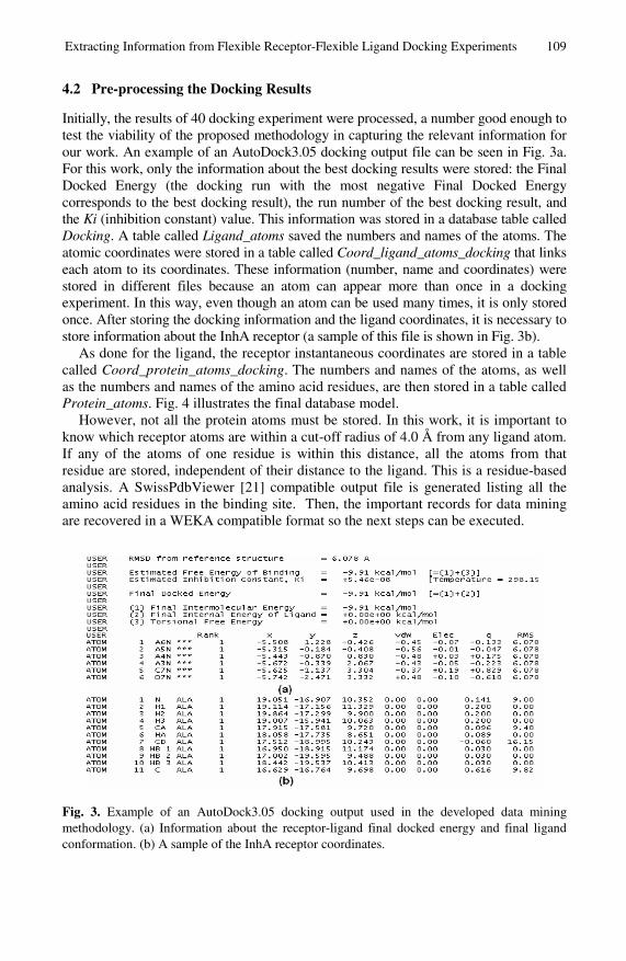
Extracting Information from Flexible Receptor-Flexible Ligand Docking Experiments 109
4.2 Pre-processing the Docking Results
Initially, the results of 40 docking experiment were processed, a number good enough to test the viability of the proposed methodology in capturing the relevant information for our work. An example of an AutoDock3.05 docking output file can be seen in Fig. 3a. For this work, only the information about the best docking results were stored: the Final Docked Energy (the docking run with the most negative Final Docked Energy corresponds to the best docking result), the run number of the best docking result, and the Ki (inhibition constant) value. This information was stored in a database table called Docking. A table called Ligand_atoms saved the numbers and names of the atoms. The atomic coordinates were stored in a table called Coord_ligand_atoms_docking that links each atom to its coordinates. These information (number, name and coordinates) were stored in different files because an atom can appear more than once in a docking experiment. In this way, even though an atom can be used many times, it is only stored once. After storing the docking information and the ligand coordinates, it is necessary to store information about the InhA receptor (a sample of this file is shown in Fig. 3b).
As done for the ligand, the receptor instantaneous coordinates are stored in a table called Coord_protein_atoms_docking. The numbers and names of the atoms, as well as the numbers and names of the amino acid residues, are then stored in a table called Protein_atoms. Fig. 4 illustrates the final database model.
However, not all the protein atoms must be stored. In this work, it is important to know which receptor atoms are within a cut-off radius of 4.0 Å from any ligand atom. If any of the atoms of one residue is within this distance, all the atoms from that residue are stored, independent of their distance to the ligand. This is a residue-based analysis. A SwissPdbViewer [21] compatible output file is generated listing all the amino acid residues in the binding site. Then, the important records for data mining are recovered in a WEKA compatible format so the next steps can be executed.
Fig. 3. Example of an AutoDock3.05 docking output used in the developed data mining methodology. (a) Information about the receptor-ligand final docked energy and final ligand conformation. (b) A sample of the InhA receptor coordinates.

110 K.S. Machado et al.
Fig. 4. Final database model
4.3 Generating the WEKA Inputs, Applying Data Mining Techniques and Analyzing the Results
In this step, we generated a WEKA compatible output. We performed some tests, but the most important were the experiments whose WEKA output is shown in Fig. 5. The first line shows all the 20 possible natural amino acids found in proteins in a three-letter code. For each docking experiment (that corresponds to one full line in the output) saved in the database, we analyzed the occurrence of protein amino acid residues within the 4.0 Å cut-off radius. If the cut-off is satisfied, a “Y” (for yes) is printed, otherwise, “N” (for not) is printed. Thus, it is possible to discover which protein amino acid residues interact with the ligand in each different protein conformation (for each saved docking result). This knowledge is very important to identify the amino acids–ligand interactions that are determining for receptor-ligand binding and affinity. With this information it is possible, for instance, to discover other ligands that interact with this protein in a similar manner. When this generated output is opened in WEKA, without applying any data mining technique, it is possible to identify the total number of experiments in which each of the residues appears.
This result can be seen in Fig. 6. From the graphics we can conclude, for example, that the amino acid residues PHE, LEU, ILE, GLY, and ALA are present in the binding site in all the stored docking experiments.
After this initial analysis, we decided to apply the association technique offered by WEKA to find association rules linking the amino acids in the protein. We

Extracting Information from Flexible Receptor-Flexible Ligand Docking Experiments 111
Fig. 5. Output from WEKA showing, in the first line, the 20 natural amino acid residues in a three-letter code. The following lines, each corresponding to a different docking experiment, show which of the 20 types of amino acid residues are present in each different docked conformation. For simplicity, only 10 conformations (docking experiments) are illustrated.
0 10 20 30 40 50
TRP
ASN
CYS
GLU
HIE
TYR
VAL
ARG
GLN
ASP
LYS
PRO
THR
MET
SER
ALA
GLY
ILE
LEU
PHE
Amino acids
Total number of docking experiments
Fig. 6. Initial results of our data mining methodology for 40 docking experiments. PHE, LEU, ILE, GLY, and ALA amino acid residues from InhA are interacting with the NADH ligand in all experiments.
Table 1. Association rules’ parameters used in WEKA
Option Function Value
-N Define the maximum number of rules to be found 50
-C Minimum metric score. Consider only rules with scores higher than this threshold
0.75
-D Iteratively decrease support 0.05
-U Upper bound for minimum support 1.0
-M Lower bound for minimum support 0.1
-T Name of training set 0
have chosen to use association rules for it is a convenient technique to verify co-occurrences of objects (amino acids) [8]. The initial parameters are described in Table 1. In particular, the minimum threshold was 10% (0.1).
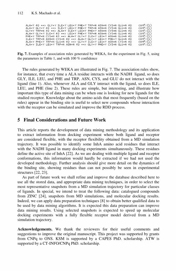
112 K.S. Machado et al.
Fig. 7. Examples of association rules generated by WEKA, for the experiment in Fig. 5, using the parameters in Table 1, and with 100 % confidence
The rules generated by WEKA are illustrated in Fig. 7. The association rules show, for instance, that every time a ALA residue interacts with the NADH ligand, so does GLY, ILE, LEU, and PHE and TRP, ASN, CYS, and GLU do not interact with the ligand (line 1). Also, whenever ALA and GLY interact with the ligand, so does ILE, LEU, and PHE (line 2). These rules are simple, but interesting, and illustrate how important this type of data mining can be when one is looking for new ligands for the studied receptor. Knowledge about the amino acids that most frequently (based on the rules) appear in the binding site is useful to select new compounds whose interaction with the receptor can be simulated and improve the RDD process.
5 Final Considerations and Future Work
This article reports the development of data mining methodology and its application to extract information from docking experiment where both ligand and receptor are considered flexible, with the receptor flexibility obtained from a MD simulation trajectory. It was possible to identify some InhA amino acid residues that interact with the NADH ligand in many docking experiments simultaneously. These residues define the active site of InhA [22]. As we are dealing with multiple ligand and receptor conformations, this information would hardly be extracted if we had not used the developed methodology. Further analysis should give more detail on the dynamics of the binding site, showing residues than can not possibly be seen in experimental structures [22, 23].
As part of future work we shall refine and improve the database described here to use all the stored data, and appropriate data mining techniques, in order to select the most representative snapshots from a MD simulation trajectory for particular classes of ligands. In special, we intend to treat the following data: catalogued compounds from ZINC [24], snapshots from MD simulations, and molecular docking results. Indeed, we can apply data preparation techniques [8] to obtain better qualified data to be used by data mining algorithms. It is expected this data preparation can improve data mining results. Using selected snapshots is expected to speed up molecular docking experiments with a fully flexible receptor model derived from a MD simulation trajectory. Acknowledgements. We thank the reviewers for their useful comments and suggestions to improve the original manuscript. This project was supported by grants from CNPq to ONS. KSM is supported by a CAPES PhD. scholarship. ATW is supported by a CT-INFO/CNPq PhD. scholarship.
Extracting Information from Flexible Receptor-Flexible Ligand Docking Experiments 113
References
1. Wang, J., Zaki, M., Toivonen, H., Shasha, D.: Data Mining in Bioinformatics. In: Advanced Information and Knowledge Processing. Springer, Heidelberg (2005)
2. Benson, D.A., Karsch-Mizrachi, I., Lipman, D.J., Ostell, J., Wheeler, D.L.: GenBank. Nucl. Acids Res. 33, 34–38 (2005)
3. Han, J.: How can Data Mining help Bio-Data Analysis? In: Workshop on Data Mining in Bioinformatics (with SIGKDD 2002 Conference) (2002)
4. Alonso, H., Bliznyuk, A.A., Gready, J.E.: Combining Docking and Molecular Dynamic Simulations in Drug Design. Med. Res. Rev. 26, 531–568 (2006)
5. Schroeder, E.K., Basso, L.A., Santos, D.S., Norberto de Souza, O.: Molecular Dynamics Simulation Studies of the Wild-Type, I21V, and I16T Mutants of Isoniazid-Resistant Mycobacterium tuberculosis Enoyl Reductase (InhA) in Complex with NADH: Toward the Understanding of NADH-InhA Different Affinities. Biophys. J. 89, 876–884 (2005)
6. Waikato Environment for Knowledge, Analysis (accessed, March 2008), http:// www.cs.waikato.ac.nz/ml/weka
7. Piatetsky-Shapiro, G., Frawley, W.J.: Knowledge Discovery in Databases. AAAI/MIT Press (1991)
8. Tan, P., Steinbach, M., Kumar, V.: Introduction to Data Mining. Person Addison Wesley (2006)
9. Fayyad, U.M., Piatetsky-Shapiro, G., Smyth, P.: The KDD Process for Extracting Useful Knowledge from Volumes of Data. Communications of the ACM 39, 27–34 (1996)
10. Drews, J.: Drug discovery: A historical perspective computational methods for biomolecular docking. Curr. Opin. Struct. Biol. 6, 402–406 (1996)
11. Lybrand, T.P.: Ligand-protein docking and rational drug design. Curr. Opin. Struct. Biol. 5, 224–228 (1995)
12. Kuntz, I.D.: Structure-based strategies for drug design and discovery. Science 257, 1078–1082 (1992)
13. Goodsell, D.S., Olson, A.J.: Automated docking of substrates to proteins by simulated annealing. Proteins 8, 195–202 (1990)
14. Huang, S., Zou, X.: Ensemble Docking of Multiple Protein Structures: Considering Protein Structural Variations in Molecular Docking. Proteins 66, 399–421 (2007)
15. Sali, A.: 100.000 Protein Structures for the Biologist. Nat. Struct. Biol. 5, 1029–1032 (1998)
16. van Gunsteren, W.F., Berendsen, H.J.C.: Computer Simulation of Molecular Dynamics Methodology, Applications and Perspectives in Chemistry. Angew. Chem. Int. Engl. Ed. 29, 992–1023 (1990)
17. Schroeder, E.K., Norberto de Souza, O., Santos, D.S., Blanchard, J.S., Basso, L.A.: Drugs that inhibit mycolic acids biosynthesis in Mycobacterium tuberculosis. Curr. Pharm. Biotech. 3, 197–225 (2002)
18. Machado, K.S., Schroeder, E.K., Ruiz, D.D., Norberto de Souza, O.: Automating Molecular Docking with Explicit Receptor Flexibility Using Scientific Workflows. In: Sagot, M.-F., Walter, M.E.M.T. (eds.) BSB 2007. LNCS (LNBI), vol. 4643, pp. 1–11. Springer, Heidelberg (2007)
19. Morris, G.M., Goodsell, D.S., Halliday, R.S., Huey, R., Hart, W.E., Belew, R.K., Olson, A.J.: Automated Docking Using a Lamarckian Genetic Algorithm and Empirical Binding Free Energy Function. J. Comput. Chem. 19, 1639–1662 (1998)
20. Frank, E., Hall, M., Trigg, L., Holmes, G., Witten, I.H.: Data Mining in Bioinformatics using Weka. Bioinformatics 20, 2479–2481 (2004)

114 K.S. Machado et al.
21. Guex, N., Peitsch, M.C.: SWISS-MODEL and the Swiss-PdbViewer: An environment for comparative protein modeling. Electrophoresis 18, 2714–2723 (1997)
22. Dessen, A., Quémard, A., Blanchard, J.S., Jacobs Jr., W.R., Sacchettini, J.C.: Crystal structure and function of the isoniazid target of Mycobacterium tuberculosis. Science 267, 1638–1641 (1995)
23. Berman, H.M., Westbrook, J., Feng, Z., Gilliland, G., Bhat, T.N., Weissig, H., Shindyalov, I.N., Bourne, P.E.: PDB - Protein Data Bank. Nucl. Acids Res. 28, 235–242 (2000)
24. Irwin, J.J., Shoichet, B.K.: ZINC - A Free Database of Commercially Available Compounds for Virtual Screening. J. Chem. Inf. Model. 45, 177–182 (2005)
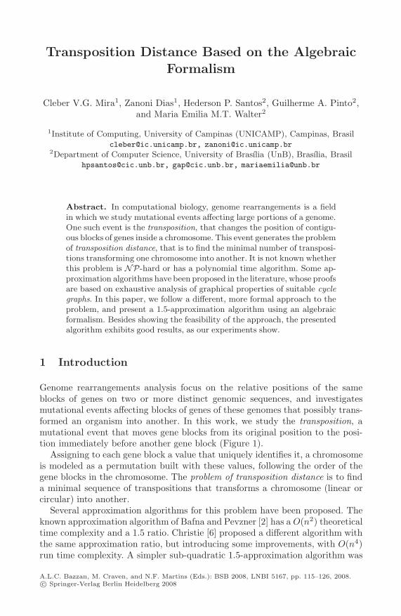
Transposition Distance Based on the Algebraic
Formalism
Cleber V.G. Mira1, Zanoni Dias1, Hederson P. Santos2, Guilherme A. Pinto2,and Maria Emilia M.T. Walter2
1Institute of Computing, University of Campinas (UNICAMP), Campinas, [email protected], [email protected]
2Department of Computer Science, University of Brasılia (UnB), Brasılia, [email protected], [email protected], [email protected]
Abstract. In computational biology, genome rearrangements is a fieldin which we study mutational events affecting large portions of a genome.One such event is the transposition, that changes the position of contigu-ous blocks of genes inside a chromosome. This event generates the problemof transposition distance, that is to find the minimal number of transposi-tions transforming one chromosome into another. It is not known whetherthis problem is NP-hard or has a polynomial time algorithm. Some ap-proximation algorithms have been proposed in the literature, whose proofsare based on exhaustive analysis of graphical properties of suitable cyclegraphs. In this paper, we follow a different, more formal approach to theproblem, and present a 1.5-approximation algorithm using an algebraicformalism. Besides showing the feasibility of the approach, the presentedalgorithm exhibits good results, as our experiments show.
1 Introduction
Genome rearrangements analysis focus on the relative positions of the sameblocks of genes on two or more distinct genomic sequences, and investigatesmutational events affecting blocks of genes of these genomes that possibly trans-formed an organism into another. In this work, we study the transposition, amutational event that moves gene blocks from its original position to the posi-tion immediately before another gene block (Figure 1).
Assigning to each gene block a value that uniquely identifies it, a chromosomeis modeled as a permutation built with these values, following the order of thegene blocks in the chromosome. The problem of transposition distance is to finda minimal sequence of transpositions that transforms a chromosome (linear orcircular) into another.
Several approximation algorithms for this problem have been proposed. Theknown approximation algorithm of Bafna and Pevzner [2] has a O(n2) theoreticaltime complexity and a 1.5 ratio. Christie [6] proposed a different algorithm withthe same approximation ratio, but introducing some improvements, with O(n4)run time complexity. A simpler sub-quadratic 1.5-approximation algorithm was
A.L.C. Bazzan, M. Craven, and N.F. Martins (Eds.): BSB 2008, LNBI 5167, pp. 115–126, 2008.c© Springer-Verlag Berlin Heidelberg 2008
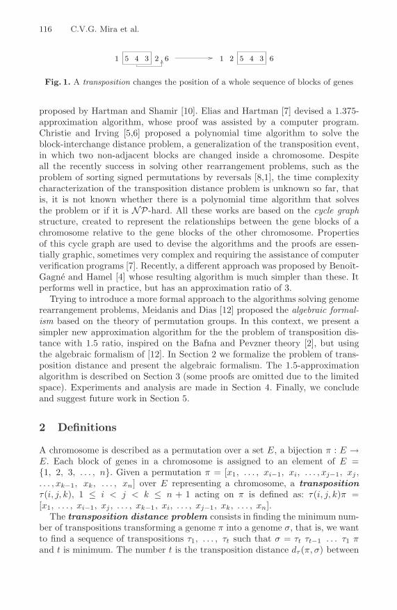
116 C.V.G. Mira et al.
1 2 6 1 2 635 4 35 4
Fig. 1. A transposition changes the position of a whole sequence of blocks of genes
proposed by Hartman and Shamir [10]. Elias and Hartman [7] devised a 1.375-approximation algorithm, whose proof was assisted by a computer program.Christie and Irving [5,6] proposed a polynomial time algorithm to solve theblock-interchange distance problem, a generalization of the transposition event,in which two non-adjacent blocks are changed inside a chromosome. Despiteall the recently success in solving other rearrangement problems, such as theproblem of sorting signed permutations by reversals [8,1], the time complexitycharacterization of the transposition distance problem is unknown so far, thatis, it is not known whether there is a polynomial time algorithm that solvesthe problem or if it is NP-hard. All these works are based on the cycle graphstructure, created to represent the relationships between the gene blocks of achromosome relative to the gene blocks of the other chromosome. Propertiesof this cycle graph are used to devise the algorithms and the proofs are essen-tially graphic, sometimes very complex and requiring the assistance of computerverification programs [7]. Recently, a different approach was proposed by Benoıt-Gagne and Hamel [4] whose resulting algorithm is much simpler than these. Itperforms well in practice, but has an approximation ratio of 3.
Trying to introduce a more formal approach to the algorithms solving genomerearrangement problems, Meidanis and Dias [12] proposed the algebraic formal-ism based on the theory of permutation groups. In this context, we present asimpler new approximation algorithm for the the problem of transposition dis-tance with 1.5 ratio, inspired on the Bafna and Pevzner theory [2], but usingthe algebraic formalism of [12]. In Section 2 we formalize the problem of trans-position distance and present the algebraic formalism. The 1.5-approximationalgorithm is described on Section 3 (some proofs are omitted due to the limitedspace). Experiments and analysis are made in Section 4. Finally, we concludeand suggest future work in Section 5.
2 Definitions
A chromosome is described as a permutation over a set E, a bijection π : E →E. Each block of genes in a chromosome is assigned to an element of E ={1, 2, 3, . . . , n}. Given a permutation π = [x1, . . . , xi−1, xi, . . . , xj−1, xj ,. . . , xk−1, xk, . . . , xn] over E representing a chromosome, a transpositionτ(i, j, k), 1 ≤ i < j < k ≤ n + 1 acting on π is defined as: τ(i, j, k)π =[x1, . . . , xi−1, xj , . . . , xk−1, xi, . . . , xj−1, xk, . . . , xn].
The transposition distance problem consists in finding the minimum num-ber of transpositions transforming a genome π into a genome σ, that is, we wantto find a sequence of transpositions τ1, . . . , τt such that σ = τt τt−1 . . . τ1 πand t is minimum. The number t is the transposition distance dτ (π, σ) between

Transposition Distance Based on the Algebraic Formalism 117
two genomes π and σ. A particular case arises when we want to compute thetransposition distance between a genome π and the genome σ = [1, 2, . . . , n].In this case, we have the equivalent problem of sorting by transpositions. Forexample, considering the following sequence of transpositions that sorts the per-mutation π = [4, 3, 2, 1, 5], we obtain dτ (π, σ) = 3: τ(1, 4, 5)π = [1, 4, 3, 2, 5],τ(2, 4, 5)τ(1, 4, 5)π=[1, 2, 4, 3, 5], τ(3, 4, 5)τ(2, 4, 5)τ(1, 4, 5)π=[1, 2, 3, 4, 5].
2.1 Permutations
The identity permutation ι is defined by ι(x) = x for any x ∈ E. For apermutation π over E, element x is called a fixed element when π(x) = x.The support, Supp(π), of a permutation π is the subset of elements not fixed inπ. For example, in the permutation π = [0, 3, 1, 5, 4, 2] over E = {0, 1, 2, 3, 4, 5},elements 0 and 4 are fixed and Supp(π) = {1, 2, 3, 5}.
Given a permutation π over E, the orbit of an element x ∈ E in π is theset orb(x, π) = {y | y = πk(x) for some integer k}. For example, the orbit of 2in the above π is {1, 2, 3, 5}. The number of orbits of π over E is o(π, E). Anorbit is called trivial when it contains only one element, otherwise it is callednontrivial. A cycle is a permutation with at most one nontrivial orbit. A k-cycle, k > 1, is a cycle such that its nontrivial orbit has size k. We denote ak-cycle α as a sequence of numbers enclosed under parenthesis (x1 x2 . . . xk),such that α(xi) = xi+1, for 1 ≤ i ≤ k − 1, and α(xk) = x1. For example,permutation π above is a 4-cycle that can be represented by (1 3 5 2).
Given permutations π and σ over E, the product πσ is obtained as follows:for each element x ∈ E, (πσ)(x) = π(σ(x)). For instance, given π = (3 2 5 1),σ = (6 4 2), and E = {0, 1, 2, 3, 4, 5, 6}, then πσ = (1 3 2 6 4 5). The inversepermutation, π−1, is the one such that ππ−1 = ι. For example, π−1 = (1 5 2 3)is the inverse of π = (3 2 5 1).
It is a well known result that a permutation has a unique decomposition asa product of cycles with disjoint orbits. Fixed elements are omitted in the cycledecomposition representation. Two cycles are disjoint when both have disjointnon-trivial orbits or when one of the cycles is the identity. For a permutationπ, the cycle decomposition is a product of disjoint orbits that equals π. Forexample, the product (1)(2 5 3)(4 6) is the cycle decomposition of [1, 5, 2, 6, 3, 4].A k-cycle is odd if k is odd, otherwise it is an even cycle. Denote by oodd(π, E)(oeven(π, E)) the number of orbits whose size is odd (even) in the cycle decom-position of π.
2.2 Algebraic Formalism
In this section, we present the algebraic formalism to model genomes and trans-positions. Bafna and Pevzner [2] represented the initial and target permutationsusing a representation called cycle graph [2]. Analysis made on this graph allowedthe discovery of the proper transposition to apply next. So, their arguments andproofs were based on graphics. The algebraic formalism [12,14] introduced amore formal way to solve the problem of transposition distance, in which trans-positions are formalized as permutations.

118 C.V.G. Mira et al.
Let [x1, x2, . . . , xn] be a permutation over {1, 2 . . . , n} modeling a linear,unichromosomal genome. Taking E = {0, 1, . . . , n}, this genome in the algebraicformalism is represented as π = (0 x1 x2 . . . xn). Observe that a “dummyblock” zero is used in order to represent the linear genome, and that the n!circular orderings of E can be mapped to the n! permutations in the traditionalrepresentation. We will consider only unichromosomal genomes in this paper.
In the algebraic formalism, a transposition is a 3-cycle τ = (u v w), withu, v, w ∈ E. We say that this transposition is applicable to a permutation πover E if u, v and w are all in the same cycle of the cycle decomposition of πand appear in this cycle in this order u, v, w. Formally, we say that w followsv for the pair (u, π), denoted by v →u,π w, when v = πk1(u), w = πk2 (u), and0 < k1 < k2 < |orb(u, π)|. A transposition is then related to the elements of thepermutation π, instead of to the positions of these elements in π as proposed byBafna and Pevzner [2]. In the algebraic approach, to apply a transposition τ tothe genome π is to perform the product τπ.
The problem of transposition distance then consists of, given the sourceπ and the target σ chromosomes, finding a sequence of transpositions τ1, . . . , τt
such that τtτt−1 . . . τ1π = σ, τi is applicable to τi−1 . . . τ1π, 1 ≤ i ≤ t, and t isminimum.
The product σπ−1, in the algebraic formalism, produces orbits correspondingto the cycles of the cycle decomposition of the cycle graph, as proposed by Bafnaand Pevzner. The idea of Bafna and Pevzner was to transform π into σ applyingtranspositions, by creating (n + 1) cycles from the cycles already existing in thefirst cycle graph. We used the same idea in the sense that “transforming π intoσ” means “to create (n + 1) cycles from the cycles existing in σπ−1”. In thealgebraic formalism, when π = σ, σπ−1 = σσ−1 = ι that is composed of (n + 1)trivial orbits: (0)(1)(2)(3)(4)(5)(6).
Following this idea, Meidanis, Dias and Mira [12,14] proved the next tworesults. The first one says that we can create or destroy exactly 2 odd cycleswhen we apply transposition τ to permutation π. The second result proves alower bound for the transposition distance.
Lemma 1. oodd(σπ−1τ−1, E) = oodd(σπ−1, E) + x, x ∈ {0,−2, +2}.Theorem 1. dτ (π, σ) ≥ 1
2 ((n + 1) − oodd(σπ−1, E)).
3 A 1.5-Approximation Algorithm
In this section we first present some definitions and results that allowed us todevise an upper bound for the transposition distance, such that the constructiveproofs were used to show the correctness of a 1.5-approximation algorithm forthis problem.
From here on, permutations π and σ formalize two chromosomes over E, andthis will be denoted only by π and σ over E. Besides, cycle α on the cycledecomposition of σπ−1 will be referred only by cycle α on σπ−1. Given π andσ over E, a transposition τ applicable to π is a x-move when o(σπ−1τ−1) =

Transposition Distance Based on the Algebraic Formalism 119
o(σπ−1) + x. A x-move is a valid x-move if oodd(σπ−1τ−1) = oodd(σπ−1) + x.Given π and σ over E, two cycles α, |α| = k1, k1 ≥ 2, and β, |β| = k2, k2 ≥ 2,on σπ−1 are linked on the cycle decomposition of σπ−1 if x →u,π πσ−1u →u,π
σπ−1x, u ∈ orb(α, σπ−1) and x ∈ orb(β, σπ−1).Given π and σ over E, u, v, w ∈ α, |α| = k, k ≥ 3, v →u,π w, then if there is at
least one 3-cycle β = (u v w) such that o(σπ−1β−1, E) = o(σπ−1, E)+2 then α isan oriented cycle. If for all 3-cycle β = (u v w), o(σπ−1β−1, E) = o(σπ−1, E),then α is a non-oriented cycle. Given π and σ over E, let α = (u · ·) a k-cycle,k ≥ 3, and β = (x · ·) a l-cycle, l ≥ 3 and l ≤ k, be cycles on σπ−1; the cyclesα and β are crossing cycles when there are integers f1, f2, . . . , fl such thatπij (u) →u,π πfj (u) →u,π πij+1 (u), πij (u) ∈ orb(α, u), and πfj (u) ∈ orb(β, x) for1 ≤ j ≤ l < n.
Lemma 2. Given π and σ over E and a non-oriented cycle C = (x · ·y · ·z · ·) onσπ−1. For all x, y and z ∈ C, the 3-cycle τ = (z y x) with y →z,π x transformsC on a non-oriented cycle on σπ−1τ−1.
Given π and σ over E and two oriented cycles C and C′ on σπ−1, then C andC′ are non-interfering cycles if C and C′ are not crossing.
Lemma 3. Given π and σ over E, cycles C = (x ·· y ··) and D = (x′ ·· y′ ··) onσπ−1, τ a transposition applicable to π formed by three among the four elementsx, y, x′ and y′, then:
1. If cycles C and D are not linked then τ creates a non-oriented cycle onσπ−1τ−1.
2. If cycles C and D are linked then τ creates an oriented cycle on σπ−1τ−1.
Given a cycle C = (· · i · · j · ·) on σπ−1, the distance between two el-ements i, j ∈ C, denoted by d(i, j), is the least positive integer k such thatj = (σπ−1)k(i). The following lemma has a constructive proof, and indicates thevalid moves to be applied when the cycle decomposition of σπ−1 has at least oneoriented cycle.
Lemma 4. Given π and σ over E, if there is an oriented cycle on σπ−1 thenthere is a transposition τ applicable to π such that τ is a valid 2-move or thereare τ1, τ2, τ3 transpositions applied to π, τ1π, τ2τ1π, that are respectively a valid0-move, and two consecutive valid 2-moves.
Proof. If there is a valid 2-move on an oriented cycle of σπ−1, then we aredone. Now suppose that there is no valid 2-moves on σπ−1 with z →y,π x. Theintuitive idea of this proof is to test all possibilities for applying transpositionson an oriented cycle, and to show that there is only one case where an orientedcycle does not allow a valid 2-move, the last case. So, take an oriented cycle Con σπ−1. Let us build a set S = {(x y z)|x, y, z ∈ C, d(x, y) odd}, that is, S isa set of transpositions applicable to π, τ = (x y z), y →x,π z, x, y, z ∈ C, suchthat o(σπ−1τ−1) = o(σπ−1) + 2 and y = (σπ−1)k(x), k odd. This is possible,because C = (x · ·y · ·z · ·) is an oriented cycle.
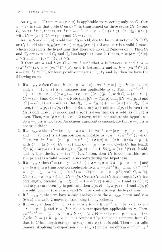
120 C.V.G. Mira et al.
As x, y, z ∈ C then τ = (y z x) is applicable to π, acting only on C, thenπ′ = τπ is such that cycle C on σπ−1 is transformed on three cycles C1, C2 andC3 on σπ−1τ−1, that is, σπ−1τ−1 = · · (· · x · · y · · z) · ·(x z y) · ·(x · ·)(y · ·)(z · ·),with C1 = (x · ·), C2 = (y · ·) and C3 = (z · ·).
As τ ∈ S and d(x, y) is odd then C2 is odd, due to the construction of S. If C1
or C3 is odd then oodd(σπ−1τ−1) = oodd(σπ−1) + 2 and so τ is a valid 2-move,which contradicts the hypothesis that there are no valid 2-moves on π. Then C1
and C3 are even and C1 and C3 has length at least 2, that is, x = (σπ−1)k(z),k ≥ 2 and z = (σπ−1)l(y), l ≥ 2.
If there are a and b on C ∈ σπ−1 such that a is between x and z, a =(σπ−1)−i1(z), a = (σπ−1)−i2 (x), or b is between z and x, b = (σπ−1)k1(z),b = (σπ−1)−k2(x), for least positive integer i1, i2, k1 and k2, then we have thefollowing cases:
1. If a →y,π x then C = (·· b ·· x ·· y ·· a ·· z) ∈ σπ−1, π = [·· y ·· b ·· z ·· a ·· x]and, τ = (y a x) is a transposition applicable to π. Then, σπ−1τ−1 =· · (· · x · · y · · a · · z)(x a y) = · · (x · · z · ·)(a · ·)(y · ·), with C1 = (x · · z · ·),C2 = (a · ·) and C3 = (y · ·). Note that |C3| = d(x, y) odd, |C2| = d(y, a) and|C1| = d(a, z) + 1 + d(z, x). But d(y, z) = d(y, a) + 1 + d(a, z) and d(y, z) iseven, then d(y, a)+d(a, z) is odd. So, as d(y, a) is odd and d(a, z) is even thenC2 is odd. If d(a, z) is odd and d(y, a) is even then C1 is odd, as d(z, x) iseven. Then, τ = (y a x) is a valid 2-move, which contradicts the hypothesis.So a →y,π x is not true. Analogous arguments demonstrate that b →y,π x isnot true either.
2. If a →x,π z then C = (x · · y · · a z b · ·) ∈ σπ−1, π = [b a · · y · · z · · x · ·]and τ = (a z x) is a transposition applicable to π, a = (σπ−1)−1(z) ∈ C.Then, σπ−1τ−1 = · · (x · · y · · a z b · ·) · ·(x z a) = · · (x b · ·)(z)(a · · y · ·),with C1 = (x b · ·), C2 = (z) and C3 = (a · · y · ·). Cycle C3 has lengthd(x, y) + d(y, a) + 1 = d(x, y) + d(y, z) − 1 + 1. So, y = (σπ−1)k(x), k odd,and by hypothesis, z = (σπ−1)l(y), l even, then C3 is odd. In this case,τ = (a z x) is a valid 2-move, also contradicting the hypothesis.
3. If b →x,π z then C = (x · · y · · a z b · ·) ∈ σπ−1, π = [b a · · y · · z · · x · ·] andτ = (b a z) is a transposition applicable to π, z = (σπ−1)(b). Then, σπ−1τ−1
= · · (x · · y · · a z b · ·) · ·(z a b) = · · (z)(a · · x · · y · ·)(b), with C1 = (z),C2 = (a · · x · · y · ·) and C3 = (b). Cycles C1 and C3 have length 1, C2 hasodd length, because C2 = d(z, x) − 1 + d(x, y) + d(y, z) − 1 and as d(z, x)and d(y, z) are even by hypothesis, then d(z, x) − 1, d(y, z) − 1 and d(x, y)are odd. So, τ = (b a z) is a valid 2-move, contradicting the hypothesis.
4. If b →x,π a, then we have a case analogous to the b →x,π z case and τ =(b a z) is a valid 2-move, contradicting the hypothesis.
5. If a →x,π b then C = (x · · y · · a z b · ·) ∈ σπ−1, π = [a · · b · · y ·· z · · x · ·], and τ = (b z x) is a transposition applicable to π. Then,σπ−1τ−1 = · · (x · · y · · a z b · ·) · ·(x z b) = · · (x b · · y · · a z · ·) · ·.Cycle C′ = (x b · ·y · ·a z · ·) is composed by the same elements from C,that is, C has length d(x, y) + d(y, z) + d(z, x) that is odd. Then τ is a valid0-move. Applying transposition τ1 = (b y x) on τπ, we obtain σπ−1τ−1τ−1
1

Transposition Distance Based on the Algebraic Formalism 121
= · · (x b · · y · · a z · ·) · ·(x y b) = · · (x · · a z · ·)(y · ·)(b) · ·, with cycle C′
transformed on cycles C1 = (x · · a z · ·), C2 = (y · ·) and C3 = (b). CycleC2 has odd length, because it is composed by the elements between x andy, C3 has length 1 and C1 has length d(y, z) + 1 + d(z, x). As d(y, z) + 1 isodd, because d(y, z) is even and as d(z, x) is even then C3 has length odd.Then, τ1 is a valid 2-move. Transposition τ2 = (a z x) transforms C1 onthe following cycles: C1τ
−12 = (x · · a z · ·)(x z a) = (x · ·)(z)(a · ·) and
C4 = (x · ·), C5 = (z) and C6 = (a · ·). Cycle C6 has length d(y, z)− 1, thatis odd. So, τ2 is a valid 2-move. ��
As could be seen on the previous theorem, there are oriented cycles that donot allow valid 2-moves. In order to avoid the creation of such cycles, we definestrongly oriented cycles. Given π and σ over E, let us take α = (x · · y · · z · ·) ak-cycle, k ≥ 3, on σπ−1, and odd d(x, y). Cycle α is strongly oriented if α isoriented and there is at least a transposition τ that is a valid 2-move. The nextlemma shows how to build a strongly oriented cycle from a non-oriented cycle.
Lemma 5. Given π and σ over E, a 3-cycle τ = (u v w) with v →u,π w, x, yand z ∈ C, such that d(x, y) odd, C = (x · · y · · z · ·) a non-oriented k-cycle,k ≥ 3, on σπ−1, and τ and C are crossing, then τ transforms C on a stronglyoriented cycle on σπ−1τ−1.
The following result shows how to create a strongly oriented cycle from twonon-oriented cycles.
Lemma 6. Given π and σ over E, with y →x′,π y′ →x′,π x, D = (x · · y · ·)and D′ = (x′ · · y′ · ·) two non-oriented cycles on σπ−1, D and D′ are notcrossing but are linked and d(x, y) is odd. Then τ formed by three among thefour elements x, y, x′ and y′ such that τ is applicable to π creates a stronglyoriented cycle.
Given π and σ over E, C a k1-cycle, k1 ≥ 3, C′ a k2-cycle, k2 ≥ 3, on σπ−1 suchthat C is strongly oriented and C′ is non-oriented, then C and C′ are stronglycrossing if C and C′ are crossing cycles.
Lemma 7. Given π and σ over E. If on σπ−1 there are strongly crossing cyclesthen we have two consecutive valid 2-moves.
Cycle C is strongly non-interfering related to cycle C′ if C and C′ arenon-interfering strongly oriented cycles.
Lemma 8. Given π and σ over E, if there are C and C′ on σπ−1 such thatC is strongly non-interfering related to C′, then there are two consecutive valid2-moves.
The following lemma shows the transpositions that must be applied when thecycle decomposition of πσ−1 has only non-oriented cycles, and at least one k-cycle, k ≥ 3.

122 C.V.G. Mira et al.
Lemma 9. Given π and σ over E, with no oriented cycles on σπ−1. If there isat least a non-oriented k − cycle, k ≥ 3, C = (x · · y · · z · ·), d(x, y) odd, thenthere are τ1, τ2 and τ3 applied to π, τ1π and τ2τ1π, respectively, such that τ1 isa valid 0-move and τ2 and τ3 are two consecutive valid 2-moves.
Proof. We have two cases.
1. Take a non-oriented, k1-cycle, k1 ≥ 3, D = (u · ·v · ·w · ·) such that
πi1 (u) →u,π πi2(u) →u,π πi3(u) →u,π πi4 (u) →u,π x
Cycles C and D are crossing, and we will denote y = πi3(u), z = πi1 (u),v = πi4(u) and w = πi2 (u), for least positive integers i3, i1, i4 and i2.Take τ = (u πi2 (u) πi4(u)) with πi2(u) →u,π πi4(u). Transposition τ is avalid 0-move because σπ−1τ−1 = · · (x · ·y · ·z · ·)(u · ·v · ·w · ·)(v w u) =· · (x · ·y · ·z · ·)(v · ·u · ·w · ·) with C′ = (x · ·y · ·z · ·), D′ = (v · ·u · ·w · ·)and τπ = (u · ·πi1 (u) · ·πi4(u) · ·x · ·πi2(u) · ·πi3 (u) · ·). Cycle C′ is stronglyoriented (Lemma 5), cycle D′ is non-oriented (Lemma 2), and C′ and D′
are crossing, so we have C′ and D′ strongly crossing. Then there are twoconsecutive valid 2-moves on σπ−1τ−1(Lemma 7).
2. Suppose that there is no cycle D such that C and D are crossing followingthe conditions of item 1. Take a non-oriented k1-cycle, k1 ≥ 2, D = (u · ·)and another non-oriented k2-cycle, k2 ≥ 2, F = (v · ·). Take u, v, w suchthat u →z,π y, v →y,π x, w →x,π z and u, w ∈ D and v ∈ F . So τ =(u v w) is such that v →u,π w and u →z,π y →z,π v →z,π x →z,π w. Then,transposition τ is applicable to π and is crossing with cycle C = (x · ·y · ·z · ·).So, τ transforms C on a strongly oriented cycle C′ on σπ−1τ−1 (Lemma 5).We have two cases (Lemma 3):(a) If D and F are linked cycles then τ creates an oriented cycle D′ on
σπ−1τ−1. Take a = (σπ−1τ−1)−j1(u), b = (σπ−1τ−1)j2(u) (on the sameconditions of Lemma 4). Lemma 4 shows that an oriented cycle is notstrongly oriented only if a →u,τπ b and w →u,τπ v. But we have v →u,τπ
on D′, and then D′ is strongly oriented. As C′ and D′ are stronglyoriented cycles on the cycle decomposition of σπ−1τ−1 and they are notcrossing then C′ and D′ are strongly non-interfering and there are twoconsecutive valid 2-moves on σπ−1τ−1 (Lemma 8).
(b) If D and F are not linked cycles then τ creates a non-oriented cycle D′
on the cycle decomposition of σπ−1τ−1 (Lemma 3). Cycles C′ and D′
do not change the crossing between cycle C and transposition τ on thecycle decomposition of σπ−1τ−1, so C′ and D′ are strongly crossing andthere are two consecutive valid 2-moves on σπ−1τ−1 (Lemma 7). ��
The following theorem shows which transpositions to apply when the cycle de-composition of σπ−1 has only k-cycles, 1 ≤ k ≤ 2, and at least two 2-cycles.
Theorem 2 (Bafna and Pevzner). Given π and σ over E, if there are onlyk-cycles, k ≤ 2, on σπ−1 then we have a valid 0-move followed by a valid 2-move.

Transposition Distance Based on the Algebraic Formalism 123
Algorithm. DistanceTransposition1.5()
Input: π, n = |π|, σOutput: τ1, ··, τk, dτ (π, σ) ≤ k ≤ 1.5dτ (π, σ)
j = 0; πj = πwhile (there is a cycle C on σπ−1
j , |C| ≥ 3) and (πj �= σ) do
while there is an oriented cycle C on σπ−1j do
j++ {Lemma 4}if there is a valid 2-move τ on C then
πj = τπj−1
elseπj = τ1πj−1 Apply a valid 0-move τ1; {Lemma 4, case 5}j++; πj = τ2πj−1 Apply a valid 2-move τ2
j++; πj = τ3πj−1 Apply a valid 2-move τ3
end ifend whilewhile (there is a non-oriented cycle C = (x · ·y · ·z · ·), |C| ≥ 3, on σπ−1
j ) and(πj �= σ) do
{Lemma 9}if there is a cycle D = (u · ·v · ·w · ·), |D| ≥ 3, C and D are crossing accordingto the conditions of item 1 of Lemma 9 then
j++; πj = τ1πj−1 Apply a valid 0-move τ1 {Lemma 7}j++; πj = τ2πj−1 Apply a valid 2-move τ2
j++; πj = τ3πj−1 Apply a valid 2-move τ3
elseTake two non-oriented cycles D = (u · ·) and F = (v · ·) according toconditions of item 2 of Lemma 9if D and F are linked cycles then
j++; πj = τ1πj−1 Apply a valid 0-move τ1 {Lemmas 4 and 8}j++; πj = τ2πj−1 Apply a valid 2-move τ2
j++; πj = τ3πj−1 Apply a valid 2-move τ3
elsej++; πj = τ1πj−1 Apply a valid 0-move τ1 {Lemmas 3 and 7}j++; πj = τ2πj−1 Apply a valid 2-move τ2
j++; πj = τ3πj−1 Apply a valid 2-move τ3
end ifend if
end whileend whilewhile (there are k-cycles, k ≤ 2 on σπ−1
j ) and (πj �= σ) doj++; πj = τ1πj−1 Apply a valid 0-move τ1 on two linked 2-cycles {Theorem 2}j++; πj = τ2πj−1 Apply a valid 2-move τ2 on the strongly oriented cycle
end while
Lemmas 4, 9 and Theorem 2 prove the correction of the algorithm Distance-Transposition1.5 and lead to the following upper bound for dτ (π, σ).
Theorem 3. dτ (π, σ) ≤ 34 ((n + 1) − oodd(σπ−1, E)).
Theorems 3 and 1 show the 1.5 ratio of the algorithm. This algorithm wasimplemented in Java, including: the basic operations on permutations, like cycle

124 C.V.G. Mira et al.
decomposition of a permutation, product of two permutations, and norm of apermutation; and the new operations acting on the cycle decomposition of σπ−1
j ,like finding a valid 2-move on an oriented cycle, a valid 0-move that are crossingwith a non-oriented cycle, and the transpositions indicated on the proofs of thelemmas and theorems described on this section.
The space complexity of our implementation was O(kn), k = dτ (π, σ) andn = |E|, due to the k + 1 vectors to store the permutations and the k vectorsto store the transpositions. The time complexity is O(n8), due to the need fordiscovering crossing cycles on the cycle decomposition of σπ−1
j .
4 Experiments and Discussion
As a case study for our theory, we executed the DistanceTransposition1.5 algo-rithm for all permutations from length 2 to 11. These experiments were executedon a machine with Pentium 4 3GHz processor, 512Mb RAM and 40Gb rigid disk.To analyze the results, we compared the values produced by the approximationalgorithm with the transposition distance, counting the number of permutationsin which these values were different. In Table 1, columns 3 to 9 show the differ-ences between dτ (π, σ) and the value computed by many algorithms found onthe literature, as well as the values computed by our algorithms.
We executed our algorithm using a heuristic for strictly decreasing permuta-tions based on a previous result from Meidanis, Walter and Dias [13].
We can observe that our 1.5-approximation algorithm produced better re-sults when compared to the BP algorithm without heuristics [18]. Our algorithmproduced worst results when compared to BPh algorithm (Bafna and Pevzner
Table 1. Comparisons of the transposition distance with the results of the algorithmsWDM-Walter, Dias and Meidanis [17], Ch-Christie [6] with heuristics (implementedby Walter, Curado and Oliveira [16]), H-Hartman [9] (implemented by Honda [11]),BP-Bafna and Pevzner [3] (implemented by Oliveira [18]), BPh-Bafna and Pevzner [3]with heuristics (implemented by Soares [19]) and the our proposed algorithms: af15-algebraic formalism with ratio 1.5 and afh15-algebraic formalism with ratio 1.5 and asimple heuristic.
|E| number ofpermuta-tions
WDM Ch H BP BPh af15 afh15
2 2 0 0 0 0 0 0 03 6 0 0 0 0 0 0 04 24 0 0 0 0 0 0 05 120 0 0 0 0 0 0 06 720 6 0 2 0 0 0 07 5040 72 0 108 1 0 1 08 40320 1167 40 1517 135 0 133 1249 362880 14327 1182 25425 4361 490 3023 297710 3265920 - - - - 17449 69353 6929711 35925120 - - - - 0 1235108 1234709

Transposition Distance Based on the Algebraic Formalism 125
with heuristics), but this significant improvement obtained by the algorithmimplemented by Soares [19] was due to the addition of a heuristic using thebranch-and-bound technique, and it was not yet included on our implementation.Considering this, our results are very encouraging.
5 Conclusions and Future Work
In this work we presented an approximation algorithm using the algebraic formal-ism of Meidanis and Dias [12,15] to solve the problem of transposition distance.We proved an upper bound for the transposition distance that, together with apreviously proved lower bound [12,14,15], allowed us to obtain the 1.5 ratio. Be-sides, we implemented this algorithm and did experiments with all permutationsfrom lengths 2 to 11. When comparing the results produced by our algorithmswith the results produced by other knows methods, we obtained better results.New directions of research are to find new theoretical results to improve thepractical results, and to lower the ratio from 1.5 to 1.375, using computationalstrategies, as suggested by Elias and Hartman [7]. We also could lower the timecomplexity of our algorithms that, although acceptable in practice, is theoreti-cally too high. Another interesting way of research is to find the transpositiondiameter. Finally we want to use the algebraic formalism to model other mu-tational events on genome rearrangements, which could contribute to create anunified approach involving different kinds of rearrangement events.
References
1. Bader, D.A., Moret, B.M.E., Yan, M.: A linear-time algorithm for computing in-version distance between signed permutations with an experimental study. Journalof Computational Biology 8(5), 483–491 (2001)
2. Bafna, V., Pevzner, P.A.: Sorting by transpositions. In: Proceedings of the SixthAnnual ACM-SIAM Symposium on Discrete Algorithms, San Francisco, USA, Jan-uary 1995, pp. 614–623 (1995)
3. Bafna, V., Pevzner, P.A.: Sorting by transpositions. SIAM Journal on DiscreteMathematics 11(2), 224–240 (1998)
4. Benoıt-Gagne, M., Hamel, S.: A new and faster method of sorting by transpositions.In: Ma, B., Zhang, K. (eds.) CPM 2007. LNCS, vol. 4580, pp. 131–141. Springer,Heidelberg (2007)
5. Christie, D.A.: Sorting permutations by block-interchanges. Information ProcessingLetters 60(4), 165–169 (1996)
6. Christie, D.A.: Genome Rearrangement Problems. PhD thesis, Glasgow University(1998)
7. Elias, I., Hartman, T.: A 1.375-approximation algorithm for sorting by transposi-tions. In: Casadio, R., Myers, G. (eds.) WABI 2005. LNCS (LNBI), vol. 3692, pp.204–215. Springer, Heidelberg (2005)
8. Hannenhalli, S., Pevzner, P.A.: Transforming men into mice (polynomial algorithmfor genomic distance problem). In: Proceedings of the 36th Annual Symposium onFoundations of Computer Science (FOCS 1995), October 1995, pp. 581–592. IEEEComputer Society Press, Los Alamitos (1995)

126 C.V.G. Mira et al.
9. Hartman, T.: A simpler 1.5-approximation algorithm for sorting by transposi-tions. In: Baeza-Yates, R., Chavez, E., Crochemore, M. (eds.) CPM 2003. LNCS,vol. 2676, pp. 156–169. Springer, Heidelberg (2003)
10. Hartman, T., Shamir, R.: A simpler and faster 1.5-approximation algorithm forsorting by transpositions. In: Proceedings of CPM 2003, pp. 156–169 (2003) (ex-tended version)
11. Honda, M.I.: Implementation of the algorithm of Hartman for the problem of sort-ing by transpositions. Master’s thesis, Department of Computer Science, Universityof Brasilia (in portuguese) (2004)
12. Meidanis, J., Dias, Z.: An alternative algebraic formalism for genome rearrange-ments. In: Sankoff, D., Nadeau, J.H. (eds.) Comparative Genomics: Empirical andAnalyitical Approaches to Gene Order Dynamics, Map Alignment and Evolutionof Gene Families, pp. 213–223. Kluwer Academic Publishers, Dordrecht (November2000)
13. Meidanis, J., Walter, M.E.M.T., Dias, Z.: Transposition distance between a per-mutation and its reverse. In: Baeza-Yates, R. (ed.) Proceedings of the 4th SouthAmerican Workshop on String Processing (WSP 1997), Valparaiso, Chile, pp. 70–79. Carleton University Press (1997)
14. Mira, C., Meidanis, J.: Algebraic formalism for genome rearrangements (part 1).Technical Report IC-05-10, Institute of Computing - University of Campinas (June2005)
15. Mira, C.V.G., Meidanis, J.: Analysis of sorting by transpositions based on alge-braic formalism. In: The Eighth Annual International Conference on Research inComputational Molecular Biology (RECOMB 2004) (March 2004)
16. Walter, M.E.M.T., Curado, L.R.A.F., Oliveira, A.G.: Working on the problem ofsorting by transpositions on genome rearrangements. In: Baeza-Yates, R., Chavez,E., Crochemore, M. (eds.) CPM 2003. LNCS, vol. 2676, pp. 372–383. Springer,Heidelberg (2003)
17. Walter, M.E.M.T., Dias, Z., Meidanis, J.: A new approach for approximating thetransposition distance. In: String Processing and Information Retrieval - SPIRE2000, pp. 199–208 (2000)
18. Walter, M.E.M.T., Oliveira, E.T.G.: Extending the theory of Bafna and Pevznerfor the problem of sorting by transpositions. Tendencias em Matematica Aplicadae Computacional - TEMA - SBMAC 3(1), 213–222 (2002) (in portuguese)
19. Walter, M.E.M.T., Soares, L.S.N., Dias, Z.: Branch-and-bound algorithms for theproblem of sorting by transpositions on genome rearrangements. In: Proceedings ofthe 26th Congress of the Brazilian Computer Society, XXXIII Seminario integradode hardware e software – SEMISH, pp. 69–81 (2006)

Using BioAgents for Supporting Manual
Annotation on Genome Sequencing Projects
Celia Ghedini Ralha1, Hugo W. Schneider1, Lucas O. da Fonseca1,Maria Emilia M.T. Walter1, and Marcelo M. Brıgido2
1 Department of Computer ScienceUniversity of Brasılia, Campus Universitario Darcy Ribeiro
Caixa Postal 4466, Brasılia-Brazil, ZipCode 70.910-900{ghedini,hugows,lucasof,mia}@cic.unb.br
2 Biology Institute, University of BrasıliaCampus Universitario Darcy Ribeiro, Brasılia-Brazil, ZipCode 70.910-900
Abstract. Enormous volume of DNA sequences of organisms are con-tinuously being discovered by genome sequencing projects around theworld. The task of identifying biological function prediction for the DNAsequences is a key activity in genome projects. This task is done in theannotation phase, which is divided into automatic and manual. The au-tomatic annotation has the objective of finding, for each DNA sequenceidentified in the project, similar sequences among millions, stored in pub-lic databases, by using approximated pattern matching algorithms. Themanual annotation is done by the biologists, that use the results pro-duced by the automatic annotation, and their knowledge and experi-ence, to decide the function prediction to each DNA sequence. In thisway, the biologists guarantee accuracy and correctness to each sequencefunction prediction. This work presents a new version of BioAgents, amultiagent system (MAS) for supporting manual annotation. The systemsimulates the biologists’ knowledge and experience for annotating DNAsequences in genome sequencing projects. The MAS cooperative ap-proach, allows to create different specialized intelligent agents that, work-ing together, suggest proper manual annotation. BioAgents was definedwith a three-layer architecture using the JADE framework with a ruler-based engine (JESS). We have done experiments with real data fromthree different genome sequencing projects: Paracoccidioides brasiliensesfungus, Paullinia cupana (guarana) plant and Anaplasma marginale rick-ettsia. The produced results were encouraging, which prove the usefulnessof BioAgents.
Keywords: manual annotation, genome sequencing projects, multia-gent system.
1 Introduction
The Human Genome Project (HGP) was one of the great feats of explorationin history, and its success encouraged the development of hundreds of genome
A.L.C. Bazzan, M. Craven, and N.F. Martins (Eds.): BSB 2008, LNBI 5167, pp. 127–139, 2008.c© Springer-Verlag Berlin Heidelberg 2008

128 C.G. Ralha et al.
projects around the world. The HGP, finished in April 2003, together with manyother genome sequencing projects, have allowed great and fast development tech-niques both on molecular biology and bioinformatics areas [30]. Since 90’s decadeit’s noteworthy the exponential growth in the volume of data generated by thesegenome sequencing projects. The management and analysis of these enormousvolume of data is one of the recent most important research focus in computerscience area, in which scientists are making great efforts to develop techniquesand software to help the biologists to store and to analyse many types of biolog-ical sequence data generated by the projects.
From a computational point of view, a DNA sequence is a string, composedwith the alphabet Σ = {A, C, G, T }, in which the characters corresponds re-spectively to the four DNA nucleotides - adenine, cytosine, guanine and thymine.Sequencing a DNA is simply to obtain the string of its nucleotides. A genomeproject is computationally supported by a pipeline composed by three phases:submission, assembly and annotation. A focus of study in the bioinformaticsarea is the improvement of the pipeline efficiency and correctness [12].
During the submission phase, the DNA sequences generated at the molecularbiology laboratories are transformed into strings, that are stored on databases,and will be used on the next phase.
At the assembly phase, the sequences are grouped according to the probabilitythat they have come from the same DNA region. Since the entire DNA can notbe sequenced at once, due to limitations of the automatic sequencers, it mustbe replicated and broken on smaller fragments. Computational tools are used togroup these fragments. A contig is a group formed by more than one sequence,having a consensus sequence to represent the group. A singlet is a group formedby an unique sequence, that could not be grouped with any other one. We willcall these contigs and singlets simply by DNA sequences, that will be used onthe next phase.
The annotation phase of a genome sequencing project has the objective ofassigning biological function prediction for the DNA sequences produced by theassembly phase. The annotation phase is divided into two tasks, automatic andmanual. The automatic annotation has the objective of finding similar sequencesto each DNA sequence discovered on the genome project, using approximatedcomparison algorithms (BLAST [17] and FASTA [31]), and databases contain-ing sequences and their corresponding function prediction (GenBank [20]). Froma query sequence, an algorithm executing on a database finds a similar DNAsequence, which means that both have approximately the same strings. The hy-pothesis is that when two DNA sequences are similar, they probably performthe same roles on the cellular mechanisms. The automatic annotation, initiallyproposes a biological function prediction for each DNA sequence. The manualannotation is done by the biologists, that decide the function prediction to eachsequence of the project, based on the outputs produced by the automatic an-notation and using their knowledge and experience. In that way, the biologistsguarantee accuracy and correctness to this task. But this work is time consum-ing, since the analysis involves many and different information sources. Thus,

Using BioAgents for Supporting Manual Annotation 129
providing computational tools to assist the manual annotation task will certainlyimprove the final annotation.
Previously, we have presented the architecture and a first prototype of BioA-gents, a system for supporting manual annotation on genome projects [27,28,29].BioAgents tool was developed with a three layer architecture using JADE frame-work [18,19] and JESS inference engine [25], for simulating the task of manualannotation as done by biologists. The MAS approach allows the interaction ofspecialized software agents in the reach of an objective [32,33]. Specialized agentsusing different approximated comparison algorithms, which interact with eachother to suggest a function prediction to a DNA sequence, may accomplish wellthe process of manual annotation.
In this article we present a new version of BioAgents, that includes a newprotocol of interaction and a more efficient execution mode in separated threads,and besides presents new experiments.
The rest of this work is divided into four sections. In Section 2 we discuss somerelated work. In Section 3 we present the architecture and the new prototype ofBioAgents. In Section 4 we describe the experiments and discuss the obtainedresults. At last, in Section 5, we conclude and suggest future work.
2 Related Work
Many projects on bioinformatics use techniques of artificial intelligence, suchas MAS, data mining and learning machines. These techniques are employedon different processes belonging to the pipeline, including genome comparisons,analysis and inferring of function prediction of genes. As far as we know, there areno projects using MAS to the manual annotation phase on genome sequencingprojects.
BioMAS system uses MAS for the automatic annotation phase of the her-pes virus [21]. The focus is the extraction of information stored on the publicdatabases and on the automatic annotation.
Electronic Annotation-EAnnot is a tool originally developed for the manualannotation of the human genome project [22]. The software combines tools toextract and analyse huge volumes of data of public databases to fastly gener-ate automatic annotation and the inference of genes. EAnnot uses informationstored in messenger RNA-mRNA, Expressed Sequence Tags-ESTs and proteinalignments, and identify pseudogenes, among other characteristics.
The tool Environment for Automatic Annotation and Comparison of Genomes- A3C [24] is based on a MAS architecture divided into two levels. Level 1 hasthe objective of integrating tasks related to the annotation phase, having toolsfor the automatic annotations of proteins. Level 2 has algorithms for genomiccomparisons, extracting useful information from level 1. The objective of A3Cis to identify relationships among different organisms. This is done by obtainingparticular characteristics of the investigated organism using the knowledge ofother organisms already sequenced and studied.
The tool Agent-based environmenT for aUtomatiC annotation of Genomes-ATUCG is based on an agent architecture, and aims to support the biologists

130 C.G. Ralha et al.
by using the concept of re-annotation [23]. In the re-annotation process, theinformation of the sequences already annotated are revised and compared tonew models and data in order to obtain characteristics and information aboutthe sequences, and annotating them again, if necessary.
3 BioAgents Improvements
As pointed in Section 1, BioAgents was developed to help biologists during themanual annotation phase of genome sequencing projects, that is a process inwhich the biologists’ knowledge and experience is used to annotate genes. Thesystem was developed to simulate the manual annotation done by biologists,using the outputs produced by the automated annotation phase, and interpretingthese results according to the knowledge stored in BioAgents.
3.1 The Architecture
In this section we describe the architecture of BioAgents, which is divided intothree layers: interface, collaborative and physical (Figure 1). The interface layerreceives the requests and returns the results to users. The collaborative layer isthe architecture core. It has specialized manager agents for executing particu-lar algorithms, like BLAST and FASTA, that interact with analyst agents fortreating specific databases, like nr [5] or kog [4]. Note that we defined specializedagents to deal with different algorithms and specific knowledge sources (KS). Atlast, this layer suggests annotations to be sent to the interface layer. The physicallayer consists of different local databases containing the results of the automaticannotation.
Fig. 1. The three layer architecture of BioAgents system

Using BioAgents for Supporting Manual Annotation 131
Following we detail the architecture layers:
– The interface layer is responsible for receiving the submitted requests, andfor returning the results for the user. The user requests consist in sending alist of sequences to be annotated.
– The collaborative layer is responsible for the suggestion of the manual anno-tation that will be returned to the interface layer, using the results producedby the analysis on the databases of the physical layer. The collaborative layeris composed by the conflict resolutions agent (CR), by the manager agents(MR) and by the analyst agents (ANL).• The CR agent has the objective to submit the requests of the interface
layer to the specialized MR agents. After receiving the results of the dis-tinct MR agents, the CR agent decides the more appropriated suggestionto be sent to the interface layer. In our case study, we used BLAST andFASTA ANL agents.
• A MR agent receives messages from the CR agent with tasks accord-ing to its expertise. A particular MR Agent verifies which databasesand program results have been previously executed in the automatic an-notation. This MR Agent allocates ANL Agents to perform particularanalysis with particular programs and databases. The MR Agent thenwaits the suggestions of all the ANL Agents, using previously definedproduction rules to consolidate these suggestions. As each MR Agent isspecialized on a particular tool, it is able to evaluate and to consolidatethe results send by its ANL Agents.
• Each ANL agent executes a particular program and uses a particulardatabase. When a request is created by a MR Agent, each ANL agentdefines a data structure, using a parser specific to the used database.This processing result with the suggestion is returned to MR Agent thatordered the request.
– The physical layer is responsible by the databases used for BioAgents. In allour case studies, we used the following data sources: nr-GenBank [16]; Ge-neOntology (GO) [7]; Clusters of Orthologous Groups of proteins (COG) [2]and the fungi databases of the nucleotide sequences of Saccharomyces cere-viseae (SC) and Schizosaccharomyces pombee (SP). The databases neededto the comparisons must be installed on the system.
3.2 The Prototype
BioAgents architecture was partially re-written, particularly a more efficientexecution mode using separated threads was developed. Like the first version, itis implemented in Java [15] with development environment Eclipse SDK, version3.1.2 [3]. Again, the used framework for the agent development is Java AgentDEvelopment Framework-JADE, version 3.4.1 [13].
Figure 2 presents a JADE ’s built-in sniffer, which is useful when debuggingagents behaviors, since it displays the messages exchanged by the sniffed agentsexecution at a specific time. The sniffer is basically a FIPA-compliant agent with
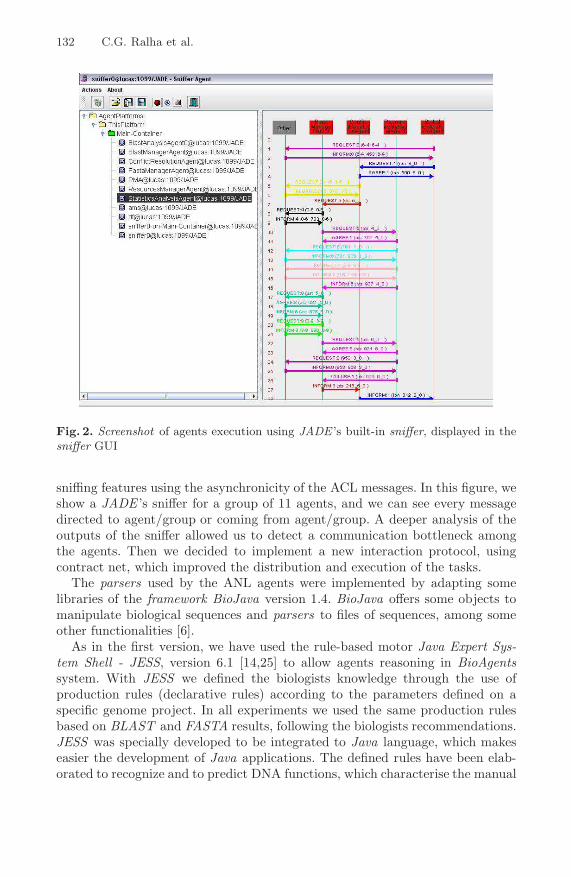
132 C.G. Ralha et al.
Fig. 2. Screenshot of agents execution using JADE ’s built-in sniffer, displayed in thesniffer GUI
sniffing features using the asynchronicity of the ACL messages. In this figure, weshow a JADE ’s sniffer for a group of 11 agents, and we can see every messagedirected to agent/group or coming from agent/group. A deeper analysis of theoutputs of the sniffer allowed us to detect a communication bottleneck amongthe agents. Then we decided to implement a new interaction protocol, usingcontract net, which improved the distribution and execution of the tasks.
The parsers used by the ANL agents were implemented by adapting somelibraries of the framework BioJava version 1.4. BioJava offers some objects tomanipulate biological sequences and parsers to files of sequences, among someother functionalities [6].
As in the first version, we have used the rule-based motor Java Expert Sys-tem Shell - JESS, version 6.1 [14,25] to allow agents reasoning in BioAgentssystem. With JESS we defined the biologists knowledge through the use ofproduction rules (declarative rules) according to the parameters defined on aspecific genome project. In all experiments we used the same production rulesbased on BLAST and FASTA results, following the biologists recommendations.JESS was specially developed to be integrated to Java language, which makeseasier the development of Java applications. The defined rules have been elab-orated to recognize and to predict DNA functions, which characterise the manual

Using BioAgents for Supporting Manual Annotation 133
annotation task, where the biologists knowledge has to be formalized, in orderto infer and suggest the annotations.
4 Experiments and Discussion
In order to validate the new version of BioAgents, we used data from threegenome sequencing projects developed at the MidWest Region of Brazil: Func-tional and Differential Genome from the Paracoccidioides brasiliensis (Pb) fun-gus [11], Genome Project of Paullinia cupana plant [9] and Genome SequencingProject of the Anaplasma marginale rickettsia [8]. We used BioAgents to sug-gest annotations for both Genome Project Pb and Genome Project Guaranausing the results of BLAST and FASTA, and comparing the suggested anno-tations with the manual annotations previously done by the biologists. Specifi-cally, for the Genome Project Pb, the analyzed data was extracted from BLASTexecuted with nr, COG and GO databases; and from FASTA with Saccha-romyces cereviseae and Schizosaccharomyces pombee fungi databases. For theGenome Project Guarana, we used BLAST executed with nr, KOG and Swis-sProt databases. The Genome Project Anaplasma was not yet manually anno-tated and we used BioAgents to support this task. For this project we usedBLAST with nr and Anaplasma marginalis St. Maries [1] databases.
To analyse the outputs from BLAST and FASTA, BioAgents used two pa-rameters, the expectation-value (e-value) and score. These parameters expressthe similarity between each sequence generated on the project with each se-quence stored on the database. Both programs produce alignments between twosequences, which express their similarity by showing the correspondence amongnucleotides from one sequence relative to the other. As lower is the e-value aslower is the error probability between the correspondences of both sequence ofnucleotides, and as higher is the score more close are the sequences. The anno-tation of each sequence is based on the similarity between both sequences, andthe hypothesis is that as much closer are the sequences as higher is the chancethat both have the same biological function prediction.
Figure 3 shows the syntax of the two rules used by JESS. We note that thesetwo rules were tested with the MR and ANL agents, using programs BLASTand FASTA. The rules described on this figure capture the following biologicalknowledge, which are pointed by (1), (2) and (3) in the figure:
– Verify if there are alignments having e-value less than or equal to 10−5 (valueadopted by the biologists on the three genome projects);
– Among the alignments following the above restriction, select the lower e-value;
– If the e-values have the same values, select the alignment with the higherscore.
From the Genome Project Pb, 6, 107 sequences were analyzed (Table 1). Fromthese, 3, 774 genes were manually annotated by the biologists, and 2, 333 werenot. Note that 3, 502 annotations were suggested by BioAgents, being 1, 547 cor-rect when compared with the 3, 774 manual annotations of the Genome Project

134 C.G. Ralha et al.
(defglobal ?*maxEvalue* = 1.0E-5); (1)
(defmodule Evalue)
(defrule Exists Evalue Above Limit"Activate GoodEvalueAnalysis module if there is at least one good evalue"(exists (BlastHit
(HitEvalue ?evalue&:(<= ?evalue ?*maxEvalue*)) (2)))=>(focus GoodEvalueAnalysis)(run)
)
(defmodule GoodEvalueAnalysis)
(defrule Best Evalue"comment"(EvalueAnalysis (Evalue ?evalue1)(Score ?score1))?fact <- (EvalueAnalysis (Evalue ?evalue2&:(>= ?evalue2 ?evalue1))
(Score ?score2&:(< ?score2 ?score1))) (3)=>(retract ?fact)
)
Fig. 3. The set of Jess rules to analyse the outputs of BLAST and FASTA
Table 1. Results of BioAgents applied to the Genome Project Pb
Number of genes 6, 107
Number of genes manually annotated 3, 774
Number of annotations suggested by BioAgents 3, 502
Number of annotations correctly indicated by BioAgents 1, 547/3, 502
Percentage of correct suggestions (related to the manual annotations) 44.1%
Number of annotations suggested for genes not manually annotated 336/2, 333
Table 2. Results of BioAgents applied on the Genome Project Guarana
Number of genes 8, 597
Number of genes manually annotated 7, 725
Number of annotations suggested by BioAgents 6, 478
Number of annotations correctly indicated by BioAgents 2, 938/6, 478
Percentage of correct suggestions (related to the manual annotations) 45.35%
Pb, which corresponds to 44.1% of correct suggestions. Observe that for the2, 333 not manually annotated genes, 336 were suggested by BioAgents. Accord-ing to the biologists, these are good results that can be improved as the agentknowledge bases are refined.
Considering the Genome Project Guarana, 8, 597 sequences were analyzed(Table 2). From these, 7, 725 genes were manually annotated by the biologists

Using BioAgents for Supporting Manual Annotation 135
Fig. 4. Results of Genome Project Pb and Genome Project Guarana
Table 3. Results of BioAgents applied on the Genome Anaplasma Project
Number of contigs 773
Number of ORFs at the contigs 1, 541
Media of ORFs on contigs 1.993
Number of annotations to ORFs (contigs) suggested by BioAgents 1, 361
Number of singlets 1, 041
Number of ORFs on singlets 1, 673
Media of ORFs on singlets 1.607
Number of annotations to ORFs (singlets) suggested by BioAgents 1, 398
Number of ORFs 3, 214
Number of ORF annotations suggested by BioAgents 2, 759
Percentage of suggestions 85.84%
and 872 were not. Note that 6, 478 annotations were suggested by BioAgents,being 2, 938 correct when compared with the 7, 725 manual annotations, whichcorresponds to 45.35% of correct suggestions.
For the Genome Project Anaplasma, BioAgents suggested 2, 759 annotationsfor a total of 3, 214 ORFs (Table 3), which corresponds to 85.84% of suggestions.This is an expected result since one of the used database was from the samealready annotated organism Anaplasma marginalis St. Maries.
Figure 4 shows the results of Genome Project Pb and Genome Project Guaranaaccording to Tables 1 and 2. Figure 5 show the results of the Genome ProjectAnaplasma according to Table 3. Figure 6 show the results of the three experi-ments. Based on the obtained results, we consider that BioAgents can really helpthe biologists on the manual annotation phase of genome sequencing projects.

136 C.G. Ralha et al.
Fig. 5. Results of Genome Project Anaplasma
Fig. 6. Percentage results of the three experiments
Using BioAgents for Supporting Manual Annotation 137
5 Conclusions and Future Work
In this article we presented a new version of BioAgents, a multiagent system tosupport the manual annotation in genome projects, that includes a new protocolof interaction and a more efficient execution mode in separated threads. Theannotation process, done by biologists on genome sequencing projects, is basedon heterogeneous and dynamic environment. It uses different and distributeddatabases, with the data being continuously modified, which fits well to themultiagent approach. BioAgents has agents specialized on distinct tasks, so thatthey can act independently, using specific rules.
Besides, we discussed the use the new version of BioAgents in three differentgenome sequencing projects: Paracoccidioides brasilienses (Pb) fungus, Paulliniacupana (guarana) plant and Anaplasma marginale rickettsia. Using a few pro-duction rules, we obtained 44.1%, and 45, 35% of correct suggestions, respec-tively on Genome Project Pb and Genome Project Guarana, computed from thenumber of correct suggestions from BioAgents when compared with the manualannotations already done on these two projects. Besides, BioAgents suggested336 annotations for not manually annotated sequences of the Project GenomePb. For Genome Project Anaplasma, BioAgents suggested 2, 759 annotationsfor 3, 214 ORFs, which represents 85.84% of manual annotations for the ORFs.This percentage was expected since Anaplasma marginalis St. Maries and nrwere used as databases for the suggestions. These results were considered verypromising by the biologists that analyzed these data.
Manual annotation is time and people consuming and its quality may bevariable according to the annotation expertise team. BioAgents may help tospeed up the annotation process and to avoid conflicts among human annota-tions. In this direction, an improvement in the expertise of the system, expressedthrough the rules, may produce a reliable, reproducible and portable annotationtool.
The majority of the related work treat the automatic annotation, like BioMASsystem and Environment for Automatic Annotation and Comparison of Genomes- A3C. Other works, like Agent-based environmenT for aUtomatiC annotation ofGenomes - ATUCG, focus on the task of re-annotation. Electronic Annotation-EAnnot treats manual annotation, specifically for the HGP. As far as we know,EAnnot does not have a reasoning mechanism to suggest annotation.
Future work include the distributed implementation for the agents, in order toreduce the time execution, and the improvement of the interface layer, providingpublic access to the researchers that want to use the system. We intend to useBioAgents in another genome project, the Genome Project Jararaca, that shortlywill start its manual annotation [10]. The improving of the knowledge of MR andANL agents is necessary to get a higher accuracy for the suggestions proposedby our system. This could be done including other methods and databases, likeHMMER/PFAM, and identification of non-coding RNAs.

138 C.G. Ralha et al.
Acknowledgements
We would like to gratefully acknowledge Richarson S. Lima for his contributionto the first version of BioAgents [26]. We also would like to thank the molecularbiology laboratory of the University of Brasılia for providing the data for theexperiments.
References
1. Anaplasma marginalis St. Maries,http://www.ncbi.nlm.nih.gov/sites/
entrez?Db=genome&Cmd=ShowDetailView&T
2. Clusters of Orthologous Groups of proteins (COG),http://www.ncbi.nlm.nih.gov/COG/
3. Eclipse SDK, http://www.eclipse.org4. kog database, http://www.ncbi.nlm.nih.gov/COG/grace/shokog.cgi5. nr database, http://www.ncbi.nlm.nih.gov/blast/blast databases.shtml
6. Framework BioJava, http://biojava.org/wiki/Main Page
7. GeneOntology (GO), http://www.geneontology.org/8. Genome Project Anaplasma,
https://www.biomol.unb.br/anaplasma/servlet/IndexServlet
9. Genome Project Guarana, https://dna.biomol.unb.br/GR/10. Genome Project Jararaca,
https://helix.biomol.unb.br/jararaca/servlet/IndexServlet
11. Genome Project Pb, https://dna.biomol.unb.br/Pb-eng/12. The IGS Annotation Engine, http://ae.igs.umaryland.edu/13. Java Agent DEvelopment Framework - JADE, http://jade.tilab.com14. Java Expert System Shell - JESS, http://www.jessrules.com/jess/index.shtml15. Java Language, http://java.sun.com16. nr-genbank, http://www.ncbi.nlm.nih.gov/Genbank/17. Altschul, S.F., Gish, W., Miller, W., Myers, E.W., Lipman, D.J.: Basic local align-
ment search tool. J. Mol. Biol. 215(3), 403–410 (1990)18. Bellifemine, F., Caire, G., Poggi, A., Rimassa, G.: JADE - a white paper. White
Paper 3, TILAB - Telecom Italia Lab (September 2003)19. Bellifemine, F., Caire, G., Trucco, T., Rimassa, G.: Jade Programmer’s Guide
(June 2007), http://jade.tilab.com/doc/programmersguide.pdf20. Benson, D.A., Karsch-Mizrachi, I., Lipman, D.J., Ostell, J., Wheeler, D.L.: Gen-
bank. Nucleic Acids Res. 36 (Database issue) (January 2008)21. Decker, K., Zheng, X., Schmidt, C.: A multi-agent system for automated genomic
annotation. In: AGENTS 2001: Proceedings of the 5th international conference onAutonomous agents, pp. 433–440. ACM, New York (2001)
22. Ding, L., Sabo, A., Berkowicz, N., Meyer, R.R., Shotland, Y., Johnson, M.R.,Pepin, K.H., Wilson, R.K., Spieth, J.: EAnnot: A genome annotation tool usingexperimental evidence. Genome Research 14(12), 2503–2509 (2004)
23. do Nascimento, L.V., Bazzan, A.L.C.: An agent-based system for re-annotation ofgenomes. In: III Brazilian Workshop on Bioinformatics (WOB), pp. 41–48 (2004)
24. dos Santos, C.T., Bazzan, A.L.C.: Using the A3C system for annotation of keywords- a case study. In: III Brazilian Workshop on Bioinformatics (WOB), pp. 175–178(2004)
Using BioAgents for Supporting Manual Annotation 139
25. Hill, E.F.: Jess in Action: Java Rule-Based Systems. Manning Publications Co.,Greenwich (2003)
26. Lima, R.S.: Sistema multiagente para anotacao manual em projetos de sequencia-mento de genomas. Master’s thesis, Department of Computer Science, Universityof Brasılia (2007),http://monografias.cic.unb.br/dspace/handle/123456789/28/browse-title
27. Lima, R.S., Ralha, C.G., Walter, M.E.M.T., Brıgido, M.M.: A multiagent sys-tem to help manual annotation on genome sequencing projects. In: IWGD2005: Proceedings of the International Workshop on Genomic Databases (2005),http://www.biowebdb.org/iwgd05/proceedings/multiagent-system.pdf
28. Lima, R.S., Ralha, C.G., Walter, M.E.M.T., Schneider, H.W., Pereira, A.G.F.,Brıgido, M.M.: BioAgents: A multiagent system for manual annotation on genomesequencing projects. In: IWGD 2007: Proceedings of the International Workshopon Genomic Databases (2007),http://bsb2007.inf.puc-rio.br/index.php?pg=home
29. Lima, R.S., Ralha, C.G., Walter, M.E.M.T., Schneider, H.W., Pereira, A.G.F.,Brıgido, M.M.: BioAgents: Um sistema multiagente para anotacao manual em pro-jetos de sequenciamento de genomas. In: ENIA 2007: 6th Brazilian Meeting on Arti-ficial Intelligence, Brazil, pp. 1302–1310 (2007), http://www.sbc.de9.ime.eb.br/
30. Liolios, K., Tavernarakis, N., Hugenholtz, P., Kyrpides, N.: The Genomes On LineDatabase (GOLD) v.2: a monitor of genome projects worldwide. Nucleic AcidsResearch 34, 332–334 (2006) (Database-Issue)
31. Pearson, W.R., Lipman, D.J.: Improved tools for biological sequence comparison.Proceedings of the National Academy of Sciences of the USA 85, 2444–2448 (1988)
32. Weiss, G.: Multiagent Systems: A Modern Approach to Distributed Artificial In-telligence. The MIT Press, Cambridge (July 2000)
33. Wooldridge, M.: Introduction to MultiAgent Systems. John Wiley & Sons, Chich-ester (June 2002)

Application of Genetic Algorithms to the
Genetic Regulation Problem
Maria Fernanda B. Wanderley1, Joao C.P. da Silva1,Carlos Cristiano H. Borges2, and Ana Tereza R. Vasconcelos2
1 Departamento de Ciencia da Computacao, Instituto de Matematica, UniversidadeFederal do Rio de Janeiro, Caixa Postal 68.530, CEP 21941-590,
Rio de Janeiro, RJ, Brazil{mfbw,jcps}@ufrj.br
2 Laboratorio Nacional de Computacao Cientıfica, Laboratory of Bioinformatics,Av. Getulio Vargas, 333, CEP 25651-075, Petropolis, RJ, Brazil
{cchb,atrv}@lncc.br
Abstract. Gene expression is the process of decoding the information ina DNA sequence into a protein. In this process, an enzyme called RNA-polymerase transcribes DNA into messenger-RNA, which is translatedinto protein. The determinant factors to decide which protein belongs toeach cell and how much of it will be produced are the concentration ofmRNA, and the frequency mRNA is translated. Operators and regula-tors, called transcription factors, control the transcription process. Thegene regulation network consists of determining how and which tran-scription factors are positioned in some DNA sequence. In this work, weexplore the ability of genetic algorithms to search in complex spaces tofind predictions of possible units of genetic information. We propose fourapproaches to solve this problem, trying to identify the pertinent set ofparameters to be used. We use E. coli sigma 70 promoters as a study ofcase.
Keywords: Gene Regulation Network, Genetic Algorithm.
1 Introduction
One of the main concepts of molecular biology is that the actions and propertiesof each cell are determined by the proteins it contains [9]. Gene expression isthe process of decoding the information in a particular DNA sequence into aparticular protein. In this process, an enzyme called RNA polymerase transcribesDNA into mRNA (messenger RNA) which is translated into protein [9]. Thedeterminant factors to decide which protein belongs to each cell and how muchof it will be produced are the concentration of mRNA, the frequency at whichmRNA is translated, and protein stability. It is important to observe that thesynthesis of proteins affects the synthesis of DNA and RNA, since there arespecial proteins that catalyze their synthesis.
There are three kinds of genes at DNA [9]: the structurals, which codify aprotein; the operators, which control the structural genes; and the regulators,
A.L.C. Bazzan, M. Craven, and N.F. Martins (Eds.): BSB 2008, LNBI 5167, pp. 140–151, 2008.c© Springer-Verlag Berlin Heidelberg 2008

Application of Genetic Algorithms to the Genetic Regulation Problem 141
which control the operator genes. The operators and the regulators, which canbe repressors or activators, are called transcription factors (TF) because theycontrol the transcription of DNA into RNA. The repressors control the tran-scription by codifying a protein that connects to the operator gene preventingRNA-polymerase to bind at the promoter region, which indicates where the tran-scription should start. The activators work in a similar way, by binding at theoperator gene to stimulate the process of transcription.
The gene regulation network [9] consists of determining how and which tran-scription factors are positioned in some DNA sequence. These factors determinewhether some protein will or will not be produced, how much of the proteinwill be produced, and when the production of the protein from RNA tran-scribed from DNA should be stopped. The configuration of these factors is calledunit of genetic information (UGI), and determining the location of those sitesin a DNA sequence is an important task to understand the gene regulationprocess.
In this work, we propose to use genetic algorithms (GAs) to determine possiblecandidates for UGIs in a DNA sequence. We analyze different ways for encodingUGIs to be used in GAs, several fitness functions, crossover and mutation rates,and the impact of using elitism in the selection operation, trying to identify thepertinent set of parameters to be used in the prediction of UGIs. We use the E.coli sigma 70 promoter as the study of case since it is a well-known organism.
The idea of using GAs to solve this problem arose because of the capacity ofGAs to perform searches in poorly known or irregular search spaces [10], seemingto be really appropriate for the problem. We have as our objective to create anadequate codification and measurement so that a naive GA can be efficient.
Other similar works have already been done using genetic algorithms. How-ever, their approach was different from the one we present in this work. Whilewe propose the use of PATSER scores combined with GAs to find sets of TFthat could form UGIs, in [1] GAs were used to find the best position weightmatrix (PWM) for putative binding sites motif and [13] combined GAs withgreedy method in order to find transcription factor binding sites (TFBS) in aset of promoter sequences.
This work is organized as follows: In Sec. 2, we present some basic aspects ofgenetic regulation. In Sec. 3, we discuss the sequence and transcription factorsused in our work, as well as the score function used to construct the fitnessfunctions to GAs. Also, we propose strategies to use GAs in genetic regulation.In Sec. 4, we present some results, comparing the proposed strategies. In Sec. 5,we conclude this paper and offer suggestions for future research.
2 Genetic Regulation
A molecule of DNA is a double strand of nucleotides composed of a nitrogenousbase (A-adenine, G-guanine, C-cytosine and T-thymine), a sugar (deoxyribose)

142 M.F.B. Wanderley et al.
Fig. 1. Representation of one of many DNA transcription mechanisms. The transcrip-tion initiation site is represented by +1. The downstream, represented by positivenumber, indicates the direction of transcription. The upstream is represented by neg-ative numbers. Note that the coordinate of the transcription factor FNR is -40, whilethe coordinate of transcription factor CRP is +30 (Position Precedence Principle).When considering a 450 base pair long DNA sequence (Sec. 3), the relative position+1 corresponds to the absolute position 358.
and a phosphate group. In this work, we will represent DNA as an oriented line(Fig. 1). The start site or transcription-initiation site represents the base pairwhere the transcription process initiates and, by convention, is denoted by +1.Base pairs that go in the direction of the transcription, said to be downstream,are represented as positive numbers and those in the opposite direction, said tobe upstream, are represented as negative numbers [9].
In the Jacob and Monod model [9], repressors and activators, called transcrip-tion factors, and E. coli RNA-polymerase work together to regulate transcriptioninitiation. A protein-binding sequence is a sequence of bases in DNA where sometranscription factor binds to prevent (in case of a repressor) or to stimulate(in case of an activator) RNA-polymerase to bind at the promoter region toinitiate the transcription process. So, determining the position of the bindingsites in DNA is an important information to understand the genetic regulationprocess.
In [2], [3] some important characteristics of the UGIs were presented. Onesuch characteristic is the required presence of a binding sequence at the re-gion between -60 and +20. These sites are called proximal sites (highlighted inFig. 1). Another important characteristic is the existence of a pattern of posi-tion followed by the operators and regulators, called the Proximal PrecedencePrinciple, which states that the proximal operators are located at the right ofthe promoter (downstream), while the regulators are at its left (upstream).
To remote sites (outside the range of -60 and +20), the precedent relationapplied is the Positional Precedence Principle. According to this principle, atranscription factor A precedes a transcription factor B if CA < CB, where CA
is the coordinate of the base located at the center of A and CB is the coordinate ofthe nucleotide located at the center of B. For example, in Fig. 1 the transcriptionfactor FNR precedes the transcription factor CRP . These principles will be usedto analyze the results obtained.

Application of Genetic Algorithms to the Genetic Regulation Problem 143
3 Applying Genetic Algorithms to the GeneticRegulation Problem
3.1 Sequence and Transcription Factors
In our study, we used a 450 base pair long DNA sequence of the operon fixA-fixB-fixC-fixX-yaaU of the E. coli K12 genome to determine which transcriptionfactors, and their positions, appear in that sequence. We considered that theabsolute position 358 in this sequence corresponds to the relative position +1 ofthe transcription initiate site (see Fig. 1).
The list of 35 transcription factors considered is presented in Table 1.Thesearch space size of possible UGI candidates, considering this 450 base pair-longsequence and these 35 transcription factors, is of the order of 6.8 × 10¹⁶.
Each transcription factor has an associated weight matrix (Table 1), usedby the PATSER program [8] to score subsequences of the given sequence inthe regulation region. The objective is to measure how close each subsequencematches the pattern described by the matrix. This means that for a weightmatrix of size m and a given sequence of size l, we have (l−m+1) subsequencesto score.
The value in the weight matrix can be derived experimentally or from thealignment matrix [11]. In the latter case, the alignment matrix is constructedfrom a set of aligned sequences such that each position contains the number of
Table 1. Transcription Factors
Transcription Alignment matrix Transcription Alignment matrixFactor size Factor size
AraC 26 Lrp 19ArcA 17 MalT 16ArgR 25 MarA 23CaiF 29 MelR 18CpxR 24 MetJ 18CRP 30 ModE 24CysB 22 NarL 16CytR 22 NtrC 29DnaA 20 OmpR 16FadR 29 OxyR 17FIS 23 PhoB 25FNR 16 PurR 16FruR 16 Rob 23Fur 25 SoxS 19
GadX 16 TorR 18GlpR 18 TyrR 18IHF 25 XylR 29LexA 16
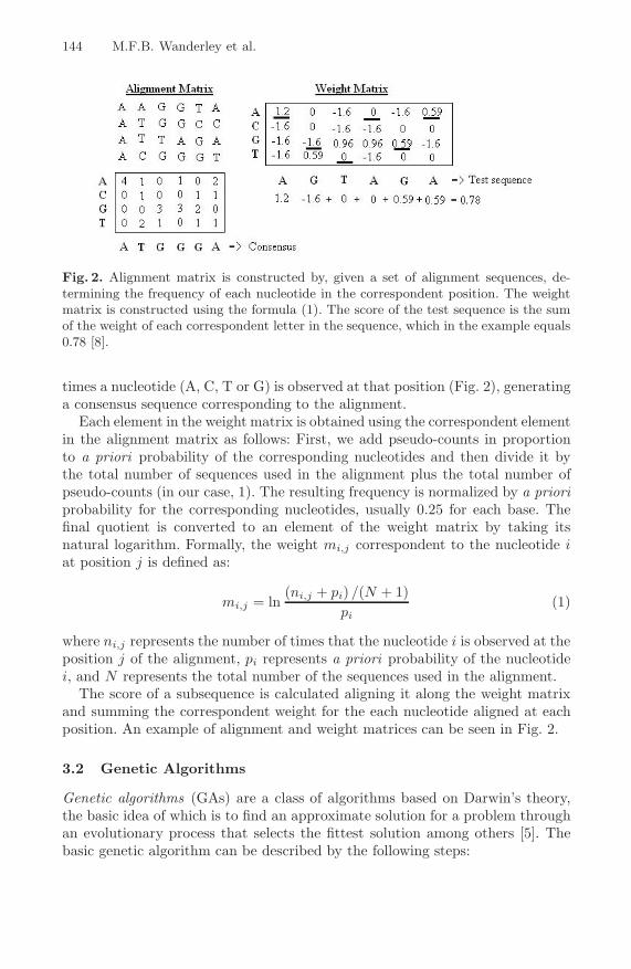
144 M.F.B. Wanderley et al.
Fig. 2. Alignment matrix is constructed by, given a set of alignment sequences, de-termining the frequency of each nucleotide in the correspondent position. The weightmatrix is constructed using the formula (1). The score of the test sequence is the sumof the weight of each correspondent letter in the sequence, which in the example equals0.78 [8].
times a nucleotide (A, C, T or G) is observed at that position (Fig. 2), generatinga consensus sequence corresponding to the alignment.
Each element in the weight matrix is obtained using the correspondent elementin the alignment matrix as follows: First, we add pseudo-counts in proportionto a priori probability of the corresponding nucleotides and then divide it bythe total number of sequences used in the alignment plus the total number ofpseudo-counts (in our case, 1). The resulting frequency is normalized by a prioriprobability for the corresponding nucleotides, usually 0.25 for each base. Thefinal quotient is converted to an element of the weight matrix by taking itsnatural logarithm. Formally, the weight mi,j correspondent to the nucleotide iat position j is defined as:
mi,j = ln(ni,j + pi) /(N + 1)
pi(1)
where ni,j represents the number of times that the nucleotide i is observed at theposition j of the alignment, pi represents a priori probability of the nucleotidei, and N represents the total number of the sequences used in the alignment.
The score of a subsequence is calculated aligning it along the weight matrixand summing the correspondent weight for the each nucleotide aligned at eachposition. An example of alignment and weight matrices can be seen in Fig. 2.
3.2 Genetic Algorithms
Genetic algorithms (GAs) are a class of algorithms based on Darwin’s theory,the basic idea of which is to find an approximate solution for a problem throughan evolutionary process that selects the fittest solution among others [5]. Thebasic genetic algorithm can be described by the following steps:

Application of Genetic Algorithms to the Genetic Regulation Problem 145
1. Randomly create an initial population, which represents a set of possiblesolutions of the problem;
2. Evaluate the individuals of the population, using a fitness function thatindicates how “adapted to the environment” an individual is (meaning, hownear from a solution an individual is);
3. Generate a new population applying operators, such as selection, crossover,and mutation, to the current one;
4. Repeat steps 2-3 until a stop condition is reached.
Several parameters need to be set prior to using GAs. Some examples are: (i)how to encode the individuals, (ii) which is the suitable fitness function usedto measure how fit an individual is to the problem, (iii) which crossover andmutation rates to use, and (iv) whether to use elitism (which means to keep oneor more of the best individuals from the current population to the next one).
3.3 Proposed Strategies
We will present here four strategies to represent individuals and to apply GAsto the Genetic Regulation Problem. Our objective is to find a solution (or solu-tions) for this problem by maximizing the scores related to position and sometranscription factor at a pre-determined sequence. None restriction were madein order to respect the obligation of the presence of at least one factor at theproximal site nor to prevent the overlap of factors. Our objective was to see ifGA was able to generate UGIs without restrictions.
As follows, TFi represents a transcription factor from Table 1, POSi rep-resents the position of the transcription factor TFi on the 450 bp-long DNAsequence used, and SCR(TFi, POSi) represents the score of TFi at the positionPOSi given by PATSER [8].
In the first strategy, the individuals were represented as binary strings of 90bits, the first 36 represented 6 transcription factors and the rest of the bitswere used to represent the positions of those factors on the 450 bp-long DNAsequence. The individuals are represented in the following way: TF1 . . . TF6
POS1 . . . POS6. An example of an individual represent by this strategy, afterdecoding from its binary form, is [empty, empty, NarL, NarL, CaiF, CpxR,150, 163, 322, 71, 217, 154]. The evaluation function is given by summing thescores given by PATSER [8] for the codified factors and correspondent positions.If the factors or positions codified on the individual were not valid or did nothave a positive score, then no value was summed on the evaluation function.Mathematically, the evaluation function can be expressed by:
EF1 = 1 + SCORE(TF1, POS1) + . . . + SCORE(TF6, POS6) (2)
One difficulty of this strategy is the number of invalid transcription factorsand positions that it can generate. Using those 6 bits to represent transcriptionfactors, we can generate 26 = 64 different transcription factors but there are only35 factors to be used; therefore, 29 of the generated elements are invalid. The

146 M.F.B. Wanderley et al.
same happened for the positions, where we have 29 = 512 generated positionsbut we have only 450 positions to address.
In the second strategy, we tried to repair this problem, keeping the codificationof the individual and changing the evaluation function, to consider the numberof invalid factors generated (NTF ). A factor is considered to be an NTF if thenumber codified at the individual does not map to a transcription factor or ifits position does not have a positive score associated. In this new function, thetotal sum of scores is divided by the NTF plus one (to prevent a division byzero).
EF2 = (1+SCORE(TF1, POS1)+. . .+SCORE(TF6, POS6))/(1+NTF ) (3)
After preliminary tests, this evaluation function proved to be more suitableand, thus, it was used by the next two strategies as well.
In the next two strategies, we restricted the number of transcription factorsto 4, in order to reduce the search space and try to find better solutions. So,the number of bits necessary to represent an individual decreases to 60. In thethird strategy, we also changed the order of representation of the factors andpositions, so the individuals were represented as TF1 POS1 . . . TF4 POS4. Anexample of an individual in this strategy, after decoding from its binary form, is[CaiF 217, F IS 64, IHF 29, GlpR 273]. As we will see, this new representa-tion increased the search efficiency because the crossover operator became lessdisruptive, decreasing the probability of harming an individual with good eval-uation. Another difference between this approach and the others is the fact thatthis new codification generates only integer numbers between 0 and 35 to repre-sent transcription factors and integer numbers between 0 and 450 to representpositions, where only 0 did not represent a factor or a position.
Notwithstanding, the third strategy solved the issue of invalid factors andpositions, the number of generated positions that did not have positive scoresassociated still was quite large, on average, 95.04% of them. In the fourth strat-egy, this problem is solved and only positions with positive scores to each factorare generated.
In this last strategy, the genes of the individual that represent positions donot generate integer numbers between 0 and 450, but a real number on therange [0, 1]. In this case, an example of an individual, after decoding from itsbinary form, could be [NarL 0.9501, CaiF 0.5760, CaiF 0.231, CytR 0.398].To evaluate the individual, this real number is mapped on the number of positivescores of the transcription factor that corresponds to this position. This processallows a dynamic mapping process, since the number of positions with positivescore is different for each one of the factors.
For example, suppose that a factor has POSPS positions representing thenumber of positions that have a positive score given by PATSER. The tableposition (POSTP ), that contains the score to be used in the evaluation functionis given by:
POSTP = 1 + round(POS ∗ (POSPS − 1)) (4)
where POS represents the value position codified on the individual.

Application of Genetic Algorithms to the Genetic Regulation Problem 147
Fig. 3. Mapping between POS and POSTP . POS = 0.9501 is the position codifiedat the individual and POSTP = 8 is the position of the table that contains the realTF position on the sequence. In this case, POSPS = 8. The table with the scores wasgenerated by PATSER for the transcription factor DnaA.
Fig. 3 shows how the mapping between the real number codified on the indi-vidual and the table position is made.
All strategies are summarized in Table 2.
Table 2. Summary of the strategies
Strategy Individual Individual Size Evaluation Function
1 TF1 . . . TF6 POS1 . . . POS6 90 EF1 = 1 + SCR(TF1, POS1) + . . .
+SCR(TF6, POS6)
2 TF1 . . . TF6 POS1 . . . POS6 90 EF1 = (1 + SCR(TF1, POS1) + . . .
+SCR(TF6, POS6))/(1 + NTF )
3 TF1 POS1 . . . TF4 POS4 60 EF1 = (1 + SCR(TF1, POS1) + . . .
+SCR(TF4, POS4))/(1 + NTF )
4 POST P = 1 + round(POS∗ 60 EF2 = (1 + SCR(TF1, POS1) + . . .
(POSP S − 1)) +SCR(TF4, POS4))/(1 + NTF )
4 Results
For each of the strategies explained above, we performed tests with the param-eters of Table 3. All tests used roulette-wheel selection, one-point crossover andsimple mutation, and were made with and without elitism; on those tests thatused elitism, the number of individuals preserved were 2.
After all tests had been finished, the second strategy was the one with theworst results with respect to satisfying the restrictions of have a TF at theproximal site and no overlap between TFs. This occurred because the numberof invalid factors and positions codified on the individual was large and then thesearch was inefficient. The fourth strategy was the best one in that it solved thequestion of invalid factors and positions that happened with the other strategies.
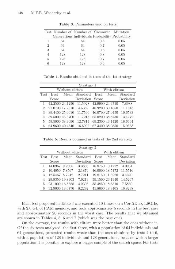
148 M.F.B. Wanderley et al.
Table 3. Parameters used on tests
Test Number of Number of Crossover MutationGenerations Individuals Probability Probability
1 64 64 0.8 0.052 64 64 0.7 0.053 64 64 0.6 0.054 128 128 0.8 0.055 128 128 0.7 0.056 128 128 0.6 0.05
Table 4. Results obtained in tests of the 1st strategy
Strategy 1
Without elitism With elitism
Test Best Mean Standard Best Mean StandardScore Deviation Score Deviation
1 42.2500 24.7250 11.5928 42.9900 24.4710 7.89882 27.0700 17.2510 4.5389 48.9200 30.1850 11.16433 39.4400 25.0010 11.7540 46.0700 27.0450 10.65334 59.5000 45.5700 11.7213 65.0200 38.8730 13.42725 59.5000 38.9090 12.7814 69.2300 43.1420 16.66646 64.9600 40.4340 16.6992 67.3400 38.0850 15.9563
Table 5. Results obtained in tests of the 2nd strategy
Strategy 2
Without elitism With elitism
Test Best Mean Standard Best Mean StandardScore Deviation Score Deviation
1 14.0967 9.2805 3.3830 18.8750 10.1772 4.00642 10.4050 7.8567 2.1874 46.0000 18.5172 11.55163 12.5467 8.7242 2.7211 19.8150 11.6220 3.43204 29.9350 19.8903 7.0213 59.1500 23.1940 14.52675 23.1000 16.8688 4.2398 35.4850 18.6510 7.58506 32.9000 18.0770 8.2292 45.8600 18.9105 10.8298
Each test proposed in Table 3 was executed 10 times, on a Core2Duo, 1.8GHz,with 2.0 GB of RAM memory, and took approximately 5 seconds in the best caseand approximately 20 seconds in the worst case. The results that we obtainedare shown in Tables 4, 5, 6 and 7 (which was the best one).
On the average, the results with elitism were better than the ones without it.Of the six tests analyzed, the first three, with a population of 64 individuals and64 generations, presented results worse than the ones obtained by tests 4 to 6,with a population of 128 individuals and 128 generations, because with a largerpopulation it is possible to explore a bigger sample of the search space. For tests

Application of Genetic Algorithms to the Genetic Regulation Problem 149
Table 6. Results obtained in tests of the 3rd strategy
Strategy 3
Without elitism With elitism
Test Best Mean Standard Best Mean StandardScore Deviation Score Deviation
1 38.3600 21.0270 6.4477 64.7900 28.3620 14.69402 40.5500 24.2740 9.8917 38.3400 24.9690 7.30783 37.3200 19.7090 7.1399 54.9000 28.2460 12.94174 71.8200 34.7350 17.3403 47.1400 34.2110 9.55715 65.4000 40.0560 16.3459 65.8600 37.9360 14.62786 57.2000 34.4800 13.1154 65.8400 40.3160 14.8843
Table 7. Results obtained in tests of the 4th strategy
Strategy 4
Without elitism With elitism
Test Best Mean Standard Best Mean StandardScore Deviation Score Deviation
1 71.8200 49.1950 13.4897 84.1500 52.7940 15.22252 64.4100 57.2060 7.5431 66.7400 47.5560 16.61953 63.6700 46.8780 11.0031 66.4400 48.8960 14.94554 84.1500 59.2260 14.3054 74.6500 66.7930 10.44475 84.1500 57.5220 14.4115 79.0300 64.4940 9.24196 86.4500 66.3950 12.9878 76.4500 66.8450 7.0611
Table 8. Statistics of the individuals generated by strategy 4 (without elitism)
Strategy 4 without elitism
Test Number of individuals Individuals Individuals Individuals with proximal
on final population with proximal site without overlapping site and no overlapping
1 64 4.68% 95.31% 4.68%2 64 10.93% 95.31% 10.93%3 64 7.81% 96.87% 7.81%4 128 21.87% 96.87% 21.87%5 128 4.68% 82.03% 4.68%6 128 14.06% 59.37% 10.93%
from 1 to 3, a greater crossover probability was more effective, while in the lastthree tests a lower probability was better.
In a preliminary analysis of the results, we verified whether there were indi-viduals that had overlapping factors and that did not have at least one factorat the proximal site. In Table 8, we show the percentage of individuals thatsatisfy these requisites for strategy 4. We chose not to make any kind of re-striction because one of our main objectives was to observe whether the ge-netic algorithm was able to generate individuals that could satisfy the biological

150 M.F.B. Wanderley et al.
requisites pointed out in [2], [3]. Besides, some individuals, such as [CaiF 164,CytR 18, CaiF 217, CaiF 274], found UGIs that have transcription factorsat nearby positions (differing by 2 bp) to the ones in the TRACTORdatabase [4], [6], [7], [12].
The presence of transcription factors on the proximal site is not guaranteedbut is observed with some individuals of the population. A factor is at theproximal site if its central nucleotide position is between positions -60 and +20,with respect to the promoter. In the sequence used in this work, the positions-60 and +20 correspond to the absolute positions 298 and 378 (Sec. 3). Forexample, the individual [CaiF 274, Fur 23, CaiF 217, GadX 343] does nothave overlapping factors and has a factor at the proximal site, GadX . This TFhas size 16 (see Table 1), so its central nucleotide is at position 343.
5 Conclusions and Future Works
In this work we proposed to generate possible candidates for UGI using geneticalgorithms from the information given by the PATSER program [8]. Some dif-ficulties were found because of the low number of positions that had a positiveevaluation compared with the number of possible positions in the DNA sequencewe used. This made us propose another strategy to deal with the position and sothe fourth strategy was the one with the best performance. We also verified thatelitism is very important to genetic algorithm success in this case. The solutionspace of this problem is complex and if we had not used elitism, individuals withgood evaluation could have been lost when we applied crossover or mutation,decreasing the mean evaluation of the population.
In future works, we intend to: (i) propose a new crossover operator to solvethe issue of invalid factors and positions generated after using this operator,(ii) propose a new mutation operator, (iii) create an evaluation function thatpenalizes individuals with overlapping, (iv) generate individuals respecting therequirement of at least one factor at the proximal site, (v) use an elitism oper-ator that preserves these individuals, and (vi) modify the stop condition of thealgorithm in order to achieve better results.
References
1. Chang, X., Zhou, W., Zhou, C., Liang, Y.: Prediction of Transcription FactorBinding Sites Using Genetic Algorithm. In: 1st IEEE Conference on IndustrialElectronics and Applications, May 24-26, 2006, pp. 1–4 (2006)
2. Collado-Vides, J.: A linguistic representation of the regulation of transcription initi-ation. i. an ordered array of complex symbols with distinctive features. BioSystems,87–104 (1993)
3. Collado-Vides, J.: A linguistic representation of the regulation of transcriptioninitiation. ii. distinctive features of sigma 70 promoters and their regulatory bindingsites. BioSystems 29, 105–128 (1993)
4. Espinosa, V., Gonzalez, A., Huerta, A., Vasconcelos, A.T., Collado-Vides, J.: Com-parative Studies of Transcriptional Regulation Mechanisms in a group of gamma-proteobacterial Genomes. J. Mol. Biol. 354, 184–199 (2005)

Application of Genetic Algorithms to the Genetic Regulation Problem 151
5. Goldberg, D.E.: Genetic Algorithms in Search, Optimization and Learning.Addison-Wesley, Massachusetts (1989)
6. Gonzalez, A., Espinosa, V., Vasconcelos, A.T., Perez-Rueda, E., Collado-Vides, J.:TRACTOR DB: a Database of Regulatory Networks in Gamma-ProteobacterialGenomes. Nucleic Acids Res. 33, D98–D102 (2004)
7. Hernandez, M., Gonzalez, A., Espinosa, V., Vasconcelos, A., Collado-Vides, J.:Complementing computationally predicted regulatory sites in Tractor DB using apattern matching approach. Silico Biology 5, 0020 (2004)
8. Hertz, G.Z., Stormo, G.D.: Identifying dna and protein patterns with statisticallysignificant alignments of multiple sequences. Bioinformatics 15(7), 563–577 (1999)
9. Lodish, H., Berk, A., Zipursky, L., Matsudaira, P., Baltimore, D., Darnell, J.:Molecular Cell Biology, 4th edn. W.H. Freedman, [S.l] (2000)
10. Michalewicz, Z.: Genetic Algorithms + Data Structures = Evolution Programs,3rd edn. Springer, Berlin (1996)
11. Stormo, G.D., Hartzell, G.W.: Identifying protein-binding sites from unaligned dnafragments. Proceedings of the National Academy of Sciences of the United Statesof America 86(4), 1183–1187 (1989)
12. Tractor db, http://www.tractor.lncc.br/13. Wang, W., Chang, X., Zhou, C.: Combining Greedy Method and Genetic Algorithm
to Identify Transcription Factor Binding Sites. In: Sixth International Conferenceon Hybrid Intelligent Systems, 2006. HIS 2006, p. 15 (December 2006)
Tests for Gene Clusters Satisfying the
Generalized Adjacency Criterion
Ximing Xu and David Sankoff
Department of Mathematics and Statistics,University of Ottawa, Ottawa, Canada K1N 6N5
{xxu060,sankoff}@uottawa.ca
Abstract. We study a parametrized definition of gene clusters that per-mits control over the trade-off between increasing gene content versusconserving gene order within a cluster. This is based on the notion of gen-eralized adjacency, which is the property shared by any two genes no far-ther apart, in the linear order of a chromosome, than a fixed thresholdparameter θ. Then a cluster in two or more genomes is just a maximalset of markers, where in each genome these markers form a connectedchain of generalized adjacencies. Since even pairs of randomly constructedgenomes may have many generalized adjacency clusters in common, westudy the statistical properties of generalized adjacency clusters underthe null hypothesis that the markers are ordered completely randomly onthe genomes. We derive expresions for the exact values of the expectednumber of clusters of a given size, for large and small values of the pa-rameter. We discover through simulations that the trend from small tolarge clusters as a function of the parameter theta exhibits a “cut-off”phenomenon at or near
√θ as genome size increases.
1 Introduction
Criteria for identifying common spatial groupings, such as synteny blocks orgene clusters, in two or more genomes entail a trade-off between increased con-tent versus stricter order: if we require genes, motifs, segments, anchors or otherelements (for which we will use the generic terms markers) of the group tobe ordered identically within different genomes, so that we can have great confi-dence that these are genuine, evolutionarily conserved or functionally determinedconfigurations, only relatively small groups are likely to satisfy this restrictivecondition, so that the analysis misses large common genomic regions that onlysuffer small, perhaps insignificant, disruptions of common order. On the otherhand, by allowing unrestricted scrambling of markers within the common groups(e.g., r-windows [2], max-gap [1] or “gene teams” [3]), we may be able to detectlarger, more loosely structured groupings, but at least in the first analysis, mustforgo accounting for local genome rearrangement, missing an important aspectof evolutionary history, and we relinquish the possibility of pinpointing extensivelocal conservation of order within the group.
We previously presented a parametrized definition of gene clusters that allowsus to control the emphasis placed on conserved order within a cluster [6] and
A.L.C. Bazzan, M. Craven, and N.F. Martins (Eds.): BSB 2008, LNBI 5167, pp. 152–160, 2008.c© Springer-Verlag Berlin Heidelberg 2008

Tests for Gene Clusters Satisfying the Generalized Adjacency Criterion 153
hence to systematically explore the details of the content/order trade-off. Thebasis for this is the notion of generalized adjacency, which is the property sharedby any two markers no farther apart, in the linear order of a chromosome, thana fixed threshold. Then a cluster in two or more genomes is just a maximalset of markers, where in each genome these markers form a connected chain ofgeneralized adjacencies. Increasing the size of the threshold relaxes the degreeof common ordering required, within a cluster, in the different genomes.
Nevertheless, for any fixed threshold, evolutionary rearrangements continueto disrupt the orders of markers on chromosome and will create, alter or destroygeneralized adjacency clusters. Since even pairs of randomly constructed genomesmay have some generalized adjacency clusters in common, the question arisesof whether the number or size of these clusters is significantly larger than therandom case. To answer such questions in this paper, we study the statisticalproperties of generalized adjacency clusters under the null hypothesis that then markers are ordered completely randomly on the genomes (N.B. it suffices torandomize just one of the genomes, since relabeling markers can convert one ofthe genome to a canonical order, e.g., 1, 2, . . . , n, without changing the number,location and size of clusters).
2 Definitions
Our definition of generalized adjacency clusters is illustrated in Figure 1.
Definition 1. Let VX to be the set of markers in the genome X. These markersare partitioned among a number of total orders called chromosomes. For mark-ers g and h in VX on the same chromosome in X, let gh ∈ EX if the number
1 2 3 4 5 6 7 8 9 10 11 12 13
14 15 16 17 18 19 20
9 6 15 8 13 12 11 18 7 10
2 5 4 1 21 19 14 3 17 16
GENOME S (3 chromosomes) GENOME T (2 chromosomes)
Generalized Adjacency Clusters:
= 2 : {2,4,5}, {6,8}, {11, 12 13}, {16, 17}= 3 : {1,2,4,5}, {6,7,8,9,10, 11, 12 13}, {14, 16, 17}= 4 : {1,2,3,4,5}, {6,7,8,9,10, 11, 12 13}, {14, 16, 17}
Fig. 1. Graphs constructed from two genomes using parameter θ = 3. Thick edgesdetermine generalized adjacency clusters. Clusters listed for θ = 2 and θ = 4 as well.
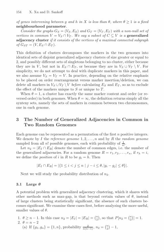
154 X. Xu and D. Sankoff
of genes intervening between g and h in X is less than θ, where θ ≥ 1 is a fixedneighbourhood parameter.
Consider the graphs GS = (VS , ES) and GT = (VT , ET ) with a non-null set ofvertices in common V = VS ∩ VT . We say a subset of C ⊆ V is a generalizedadjacency cluster if it consists of the vertices of a maximal connected subgraphof GST = (V, ES ∩ ET ).
This definition of clusters decomposes the markers in the two genomes intoidentical sets of disjoint generalized adjacency clusters of size greater or equal to2, and possibly different sets of singletons belonging to no cluster, either becausethey are in V , but not in ES ∩ ET , or because they are in VS ∪ VT \ V . Forsimplicity, we do not attempt to deal with duplicate markers in this paper, andwe also assume VS = VT = V . In practice, depending on the relative emphasisto be placed on order rearrangement versus marker insertion/deletion, we candelete all markers in VS ∪VT \V before calculating ES and ET , so as to excludethe effect of the markers unique to S or unique to T .
When θ = 1, a cluster has exactly the same marker content and order (or re-versed order) in both genomes. When θ = ∞, the definition returns simply all thesynteny sets, namely the sets of markers in common between two chromosomes,one in each genome.
3 The Number of Generalized Adjacencies in Common inTwo Random Genomes
Each genome can be represented as a permutation of the first n positive integers.We denote by I the reference genome 1, 2, . . . , n and by R the random genomesampled from all n! possible genomes, each with probability of 1
n! .Let n2 = |EI ∩ ER| denote the number of common edges, i.e. the number of
the generalized adjacencies. For a random genome R = r1, r2, . . . , rn, if rh = i,we define the position of i in R to be gi = h. Then
|EI ∩ ER| = |{1 ≤ i < j ≤ n | j − i ≤ θ, |gi − gj | ≤ θ}|.
Next we will study the probability distribution of n2.
3.1 Large θ
A potential problem with generalized adjacency clustering, which it shares withother methods such as max-gap, is that beyond certain values of θ, insteadof large clusters being statistically significant, the absence of such clusters be-comes significant. We examine these cases first, before analyzing the more useful,smaller values of θ.
1. θ ≥ n − 1. In this case n2 = |EI | = |ER| =(
n2
), so that P [n2 =
(n2
)] = 1.
2. θ = n − 2(a) If {g1, gn} = {1, n}, probability 2
n(n−1) , n2 =(n2
) − 1,
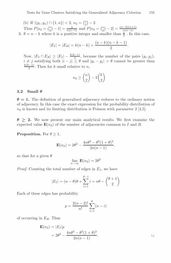
Tests for Gene Clusters Satisfying the Generalized Adjacency Criterion 155
(b) If |(g1, gn) ∩ {1, n}| < 2, n2 =(n2
) − 2.
Thus P [n2 =(n2
) − 1] = 2n(n−1) and P [n2 =
(n2
) − 2] = (n−2)(n+1)n(n−1)
3. θ = n − k where k is a positive integer and smaller than n2 . In this case,
|EI | = |ER| = k(n − k) +(n − k)(n − k − 1)
2.
Now, |EI ∩ ER| ≥ |EI | − k(k−1)2 , because the number of the pairs (gi, gj),
i = j satisfying both |i − j| ≤ θ and |gi − gj | > θ cannot be greater thank(k−1)
2 . Then for k small relative to n,
n2 ≥(
n
2
)− 2
(k
2
)
3.2 Small θ
θ = 1. The definition of generalized adjacency reduces to the ordinary notionof adjacency. In this case the exact expression for the probability distribution ofn2 is known and its limiting distribution is Poisson with parameter 2 [4,5].
θ ≥ 2. We now present our main analytical results. We first examine theexpected value E(n2) of the number of adjacencies common to I and R.
Proposition. For θ ≥ 1,
E(n2) = 2θ2 − 4nθ3 − θ2(1 + θ)2
2n(n − 1),
so that for a given θlim
n→∞E(n2) = 2θ2
Proof. Counting the total number of edges in EI , we have
|EI | = (n − θ)θ +θ−1∑
i=1
i = nθ −(
θ + 12
)
Each of these edges has probability
p =2(n − 2)!
n!
θ∑
i=1
(n − i)
of occurring in ER. Thus
E(n2) = |EI |p= 2θ2 − 4nθ3 − θ2(1 + θ)2
2n(n − 1). �

156 X. Xu and D. Sankoff
Fig. 2. Empirical distributions of the number of generalized adjacencies compared tothe related Poisson distribution for θ = 2, 5 and 10
We can say more about the limiting behaviour of n2. Indeed, we may state (proofomitted):
Proposition. For θ ≥ 1, n2 converges in distribution to a Poisson distribu-tion with parameter 2θ2.
We generated 10, 000 random permutations on 1, . . . , 100 and calculated n2 forvarious values of θ. In Figure 2, we compare the simulated distribution of n2 (withmeans indistinguishable from 2θ2 − 4nθ3−θ2(1+θ)2
2n(n−1) in each case) to the Possiondistribution with parameter 2θ2, for θ = 2, 5 and 10. For fixed n, the differ-ence is larger as θ increases, though as n increases the Poisson is the limitingdistribution.
4 Clusters of Larger Size
We use nk to denote the number of connected components of size k in EI ∩ER,with no disjointness requirement or restriction against the component beingcontained in a larger cluster. We have already studied the distribution of n2 inSection 3. We now consider the expectation of n3. Extending the approach weused in the Proposition in Section 3.2, we can list all the connected componentsof size 3 in genome I and calculate the probability it is also in R. Adding all theprobabilities together, we find

Tests for Gene Clusters Satisfying the Generalized Adjacency Criterion 157
E(n3) =θ2
n(5θ2 − 2θ − 1) + O(
1n2
)
Similarly, with additional effort, we find that
E(n4) =θ2
n2(1249
θ4 − 956
θ3 − 89θ2 +
296
θ +19) + O(
1n3
)
but the number of different kinds of components of size 5 precludes extendingour method, based on listing all possibilities, to n5 and beyond.
4.1 Testing
Despite the fact that we have only partial results for nk, we can still use standardstatistical methods to test for the relatedness of two genomes or the significanceof a generalized adjacency cluster, especially if E(n4) is small.
5 The Maximum Size Generalized Adjacency Cluster
The ideal statistic to use to test the relatedness of genomes or to detect clus-ters would be the size of the largest cluster kmax. While analytical techniqueshave not produced useful information about the distribution of kmax, it is astraightforward matter to simulate random genomes and estimate this distribu-tion empirically. Figure 3 shows the cumulative distribution functions for kmax
Fig. 3. Empirical cumulative distribution functions for kmax as a function of n and θ
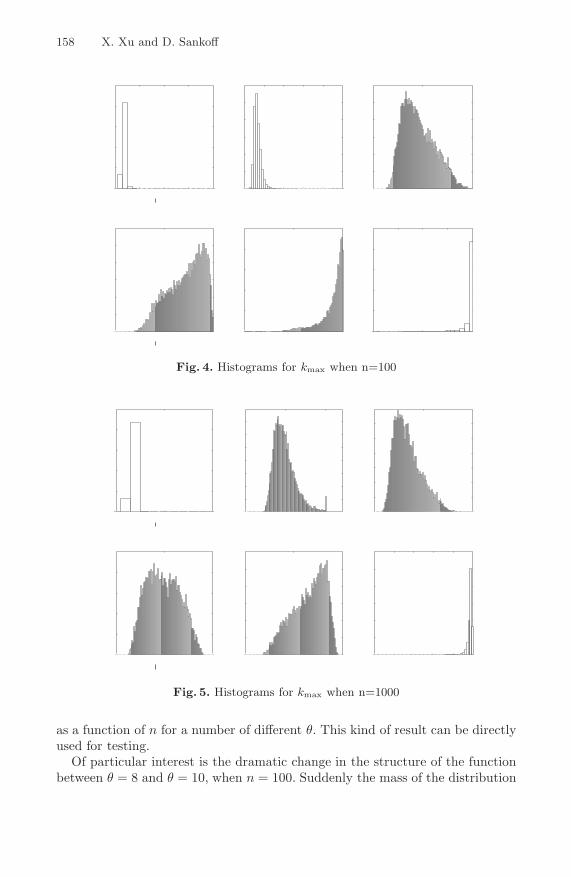
158 X. Xu and D. Sankoff
Fig. 4. Histograms for kmax when n=100
Fig. 5. Histograms for kmax when n=1000
as a function of n for a number of different θ. This kind of result can be directlyused for testing.
Of particular interest is the dramatic change in the structure of the functionbetween θ = 8 and θ = 10, when n = 100. Suddenly the mass of the distribution

Tests for Gene Clusters Satisfying the Generalized Adjacency Criterion 159
0
20
40
60
80
100
0 20 40 60 80 100
SQRT(n)
Change-point
Fig. 6. Change-point for kmax distribution as a function of√
n. Dotted diagonal rep-resents exact square root of n.
0
0.1
0.2
0.3
0.4
0.5
0.6
0.7
0.8
0.9
1
0 0.5 1 1.5
theta/SQRT(n)
Pro
port
ion o
f sim
ula
ted k
max>
0.5
n
1000
n=10 100 10000
Fig. 7. Cut-off for maximum size cluster

160 X. Xu and D. Sankoff
shifts from values around 20 to values around 75. We investigated thisphenomenon in more detail, as exemplified in Figures 4 and 5, each based on10,000 pairs of random genomes. It is remarkable how quickly the distributionchanges between θ = 9 and θ = 10 for n = 100, and between θ = 31 and θ = 33for n = 1000. On the basis of 10,000 pairs of random genomes, we determinedthe mean change-point θ∗ for a range of values of n, and in Figure 6 plottedthese points against
√n. This suggests that the change-point satisfies θ∗ =
√n
or some similar relation.To characterize the abruptness of the change around the change-point, we
calculated how much of the probability mass falls to the right of 0.5n, for eachvalue of θ. Figure 7 shows that the change behaviour, in proportion to
√n, tends
to a sharp “cut-off” at or near θ =√
n.
6 Discussion
We have begun the investigation of statistics related to generalized adjacencyclusters. The behaviour of the number of clusters for a given n and θ seemsamenable to analytical investigation, as we have demonstrated with a numberof new results. The distribution of kmax, a tool for suggesting the biologicallymost interesting clusters, does not seem as accessible, but is easily simulated.Knowledge of the cut-off behaviour serves to delimit the region for meaningfultests to θ suitably less than
√n.
Acknowledgments
Research supported in part by grants from the Natural Sciences and EngineeringResearch Council of Canada (NSERC) to DS. DS holds the Canada ResearchChair in Mathematical Genomics.
References
1. Bergeron, A., Corteel, S., Raffinot, M.: The algorithmic of gene teams. In: Guigo, R.,Gusfield, D. (eds.) WABI 2002. LNCS, vol. 2452, pp. 464–476. Springer, Heidelberg(2002)
2. Durand, D., Sankoff, D.: Tests for gene clustering. Journal of Computational Biol-ogy 10, 453–482 (2003)
3. Hoberman, R., Sankoff, D., Durand, D.: The statistical analysis of spatially clusteredgenes under the maximum gap criterion. Journal of Computational Biology 12, 1081–1100 (2005)
4. Wolfowitz, J.: Note on runs of consecutive elements. Annals of Mathematical Statis-tics 15, 97–98 (1944)
5. Xu,W., Alain, B., Sankoff, D.: Poisson adjacency distributions in genome comparison:multichromosomal, circular, signed and unsigned cases. Bioinformatics 24 (2008)
6. Zhu, Q., Adam, Z., Choi, V., Sankoff, D.: Generalized gene adjacencies, graph band-width and clusters in yeast evolution. In: Mandoiu, I., Sunderraman, R., Zelikovsky,A. (eds.) ISBRA 2008. LNCS (LNBI), vol. 4983, pp. 134–145. Springer, Heidelberg(2008)

Identity Transposon Networks in D. melanogaster
Alcides Castro-e-Silva1, Gerald Weber1, Romuel F. Machado1,Elizabeth F. Wanner2, and Renata Guerra-Sa3
1 Department of [email protected]
2 Department of Mathematics,3 Department of Biological Sciences,
Federal University of Ouro Preto, Ouro Preto-MG, Brazil
Abstract. Transposable elements, or transposons, are DNA segmentsthat are repeated within the same genome and are an important com-ponent of the genomes of most species. It is generally believed that theyplay an important role in evolution and genome restructuring. In thiswork we built a network based on a score which represents the transpo-son identity. This score is calculated by comparing all currently knownD. melanogaster transposons to each other using a Neddleman-Wunschalignment algorithm. We then use this score to build networks with trans-posons having a minimal value of identity. We start with networks oftransposons with total identity (all have score one) to networks wherethey may have any identity score (all have non-negative score). The num-ber of successful comparisons as a function of the minimal score showsan abrupt transition for minimal scores at 0.25 which can be associatedto general properties of repetitions usually found in genomes. We alsoshow that this score leads to a transition in the topology of transposonnetworks from scale-free to almost fully-connected.
Current advances in genomic sequencing generated huge amounts of data frommany species to a great degree of detail. It is now possible to access completegenomes and chromosome sequences, genes and transcriptions factors and pro-tein relations just to mention a few but important examples. The ever increasingdetails of these databases stresses the fact that it is important to understandhow their elements are related and how they interact. Interaction networks, suchas protein-protein interactions, may emerge from combining elements of thesedatabases. None of these networks are independent, they can interact with othernetworks to several degrees and on various scales, i.e., we may have a network ofnetworks and so on. Analysing the scale of the interaction network is one possi-ble way to grasp the complexity of the vast amount of information provided bythese networks. The study of interconnected elements is called graph theory andthe classical mathematical theory was developed by Erdos and Renyi [1]. Graphtheory was reborn in 1999 with the work of Barabasi and Albert who intro-duced the concept of scale-free networks [2,3]. Basically, the difference beetweenErdos-Barabasi graphs relies on equilibrium concepts. The networks studied byErdos were called random networks, in this class of graphs the number of nodes
A.L.C. Bazzan, M. Craven, and N.F. Martins (Eds.): BSB 2008, LNBI 5167, pp. 161–164, 2008.c© Springer-Verlag Berlin Heidelberg 2008

162 A. Castro-e-Silva et al.
are constant and the links are distributed with a certain probability over thosenodes. Such procedure creates equilibrium networks since all nodes have thesame statistical characteristics. On the other hand in the Barabasi model, thenodes (and its links) are added to a initial core, and the network grows (thereforecalled growing networks). Here we have a non-equilibrium graph since the nodesare not statistically equivalent and they have different ages since the nodes areintroduced at different stages of network growth. Another important feature ofBarabasi model are the rules of how the links are established: the probability ofa new node to connect to an old one is proportional to the number of connec-tions of the old node already has. This is called preferential attachment whichis also known as the rich get richer. Growing networks with preferential attach-ment lead to scale-free networks that is a special case of graph characterised bya power-law of distribution of connectivities. Following the work of Barabasi, itwas discovered that many biological networks display scale-free properties suchas the protein interaction of the gene regulatory and the metabolic system [4].
In this work we investigate the network of transposable elements or trans-posons of D. melanogaster [5,6]. We show that this similarity network has ascale-free power law. Since preferential attachment is the only known method tocreate scale-free networks this is indicative of some sort of growing mechanismshould responsible for the transposition of such repetitive elements. Indeed thisgrowing mechanism is at the very heart of the appearance of multiple copies oftransposons in genome.
We calculated the global alignment score use a standard Needleman-Wunsch al-gorithm to compare all currently known 6003 transposons of D. melanogaster [7].We used a score of i = 2 for two identical nucleotides, n = −1 for non-identicalnucleotides and g = −2 for gaps. The alignment score S resulting from theNeedleman-Wunsch algorithm takes a maximum value of iN when both sequencesof length N are identical. We use this to define a relative alignment score s =S/iNmin [Nmin = min(N1, N2)] for two sequences of length N1 and N2, such thatit becomes normalised to one for the case of fully identical sequences. Completenon-similarity sequences yield a value of s close to zero, or even negative due tothe negative alignment score for non-identical bases or gaps. To speed up the cal-culation, we have restricted the alignment to sequences whose length satisfy
|N1 − N2|max(N1, N2)
< 0.5. (1)
For the known transposons of D. Melanogaster we performed a total of 4.6×10⁶
alignments. The complete identity, s = 1, is found for transposons which occur atdifferent location within a genome or chromosome but have not yet suffered anyfurther mutation. This indicates situations where the transposition has occurredonly recently during the evolution.
Our networks are formed by nodes (transposons) and a link beetween twotransposons is added if the normalised score s is larger than a minimum score sm.For instance, with sm = 1 we obtain a network formed by transposons whichare fully identical. In Fig. 1 we show the number of transposons in a networkas function of the minimum score sm. We observe a steep transition at around

Identity Transposon Networks in D. melanogaster 163
0 0.5 1limit score sm
0
2
4
Tra
nspo
sons
with
s>
sm
/ 10
6
Fig. 1. Number transposons with normalised score s larger than a minimum score sm.The transition around sm = 0.25 is shown by vertical dashed line.
sm = 0.25 where the number of transposons in the network are reduced by twoorders of magnitude. This type of transition is known to occur in the repeatanalysis of short sequences in genomes [8]. In this type of analysis, the genomeis divided into small subsequences of a given length and each subsequence iscompared to all other subsequences of same length. For very short subsequencesthere are no unique sequences in the genome, however the transition for non-unique sequences to all sequence becoming unique happens over an interval ofjust very few nucleotides [8]. The transition shown in figure 1 is of similar origin.Even very dissimilar transposons share a number of similar subsequences due tothe occurrence of repetitions in the genome [8], therefore these repetitions giverise to the large number of scores smaller than 0.25.
We also calculated the distribution of connectivity P (k). This distribution isa histogram that shows how many nodes have k connections, results are shownin Fig. 2 for minimal score sm equal to 0.1, 0.25, 0.4 and 0.9. For sm > 0.25we observe the characteristic power-law form P (k) corresponding to scale-freenetworks. This power-law is shown as a guide-to-the-eye straight line in log-log plot. The power law distribution yields two basics features of the networkregarding the connectivity: (a) there is no characteristic node and (b) thereare few nodes with high connectivity (called hubs) and many nodes with lowconnectivity.
Work is in progress where we study the particular features of specific trans-poson families, such as the abundant INE-1 family as well as transposon classessuch as LTR retrostranposons. Also, we are currently using genetic algorithmsto optimise the Needleman-Wusch score to enhance the specificity of transposonalignment.
We thank the Brazilian agencies Fapemig and CNPq for financial support.

164 A. Castro-e-Silva et al.
1 101 102 103 1041
101
102
P(k
)(a) sm=0.1
1 101 102 103 104
(b) sm=0.25
1 101 102 1031
101
102
103
P(k
)
(c) sm=0.4
1 101 102
(d) sm=0.9
connections k
Fig. 2. Distribution of connectivities of Transposons identity for several scores (log-log plots). The power-law signature of scale-free behaviour, shown as guide-to-the-eyedashed lines, is present only for minimal scores sm larger than 0.25.
References
1. Erdos, P., Renyi, A.: On the evolution of random graphs. Publ. Math. Inst. Hung.Acad. Sci. 5, 17–61 (1960)
2. Barabasi, A., Albert, R.: Emergence of scaling in random networks. Sci-ence 286(5439), 509 (1999)
3. Barabasi, A., Oltvai, Z.: Network biology: understanding the cell’s functional orga-nization. Nature Reviews Genetics 5(2), 101–113 (2004)
4. Jeong, H., Tombor, B., Albert, R., Oltvai, Z., Barabasi, A., et al.: The large-scaleorganization of metabolic networks. Nature 407(6804), 651–654 (2000)
5. Bartolome, C., Maside, X., Charlesworth, B.: On the abundance and distribution oftransposable elements in the genome of Drosophila melanogaster. Molecular Biologyand Evolution 19(6), 926–937 (2002)
6. Rizzon, C., Marais, G., Gouy, M., Biemont, C.: Recombination rate and the distri-bution of transposable elements in the Drosophila melanogaster genome. GenomeResearch 12, 400–407 (2002)
7. Durbin, R., Eddy, S.R., Krogh, A., Mitchison, G.: Biological sequence analysis: prob-abilistic models of proteins and nucleic acids. Cambridge Univ. Press, Cambridge(2000)
8. Whiteford, N., Haslam, N., Weber, G., Prugel-Bennett, A., Essex, J.W., Roach, P.L.,Bradley, M., Neylon, C.: An analysis of the feasibility of short read sequencing. Nucl.Acids. Res. 33(19), e171 (2005)

Prediction of Protein-Protein
Binding Hot Spots:A Combination of Classifiers Approach
Roberto Hiroshi Higa1,2 and Clesio Luis Tozzi2
1 Embrapa Informatica AgropecuariaEmpresa Brasileira de Pesquisa Agropecuaria - EMBRAPA, CP 6041
13083-970 - Campinas, SP, [email protected]
http://www.cnptia.embrapa.br2 Departamento de Engenharia de Computacao e Automacao Industrial
Faculdade de Engenharia Eletrica e de Computacao, CP 6101Universidade Estadual de Campinas - UNICAMP
13083-970, Campinas, SP, Brazil{rhhiga,clesio}@dca.fee.unicamp.br
http://www.fee.unicamp.br
Abstract. In this work we approach the problem of predicting proteinbinding hot spot residues through a combination of classifiers. We con-sider a comprehensive set of structural and chemical properties reportedin the literature for characterizing hot spot residues. Each componentclassifier considers a specific set of properties as feature set and theiroutput are combined by the mean rule. The proposed combination ofclassifiers achieved a performance of 56.6%, measured by the F-Measurewith corresponding Recall of 72.2% and Precision of 46.6%. This per-formance is higher than those reported by Darnel et al. [4] for the samedata set, when compared through a t-test with a significance level of 5%.
Keywords: hot spots, combination of classifiers, protein interaction,binding sites.
1 Introduction
Protein-protein interactions play a key role in most of biological process, being ofgreat importance for living cells. Although the principles governing this processis still not fully understood, it is well-known that binding energy is not evenlydistributed among interface residues, with a large contribution coming from onlya small subset of the interface residues [10]. These residues are referenced asbinding hot spots.
The recent interest in protein-protein interface as drug targets [2] has high-lighted the importance of identifying hot spots systematically. Usually, this isdone through site-directed mutagenesis experiments like alanine scanning tech-nique [10], whose aim is to evaluate the impact on the binding energy caused
A.L.C. Bazzan, M. Craven, and N.F. Martins (Eds.): BSB 2008, LNBI 5167, pp. 165–168, 2008.c© Springer-Verlag Berlin Heidelberg 2008

166 R.H. Higa and C.L. Tozzi
by mutations to alanine of specific interface residues; but, they can demanda significant experimental effort. In this scenario, the interest for cheaper andfaster computational hot spot prediction methods grows. Such a computationalmethod can help biologists to keep the experimental effort focused only on thoseinterface residues presenting better chance to be hot spots.
In this work, we use a comprehensive set of structural and chemical proper-ties to predict binding hot spot residues through a strategy of combination ofclassifiers.
2 Material and Methods
We use a data set compiled by Darnell et al. [4]. This choice is based on thefact that this data set has been processed in order to reduce as much as possiblethe presence of low quality and/or redundant structures. We also had to removefrom the data set 15 residues for which we could not calculate the correspondingconservation score property. The following set of properties was selected in orderto characterize interface residues:
– Amino acid type of the interface residue, represented by the two indexesproposed by Hagarty et al. [6];
– Residue conservation score of the interface residue and the average score of itsneighbor residues, calculated by using the software rate4site [11] and MSA ofhomologue sequences from Swissprot/Uniprot Knowledgebase release 9.6 [1];
– Solvent accessible surface area - ASA in isolation and in complex for theinterface residue and for its neighbor residues, calculated by using programvolbl, included in the software package alpha shapes [8];
– Atomic packing scores computed for intra chain neighbors and for inter chainneighbors, defined by the occupied volume around the interface residue;
– Inter chain atomic contacts [9]; and– Computational ΔΔG value, computed by using the Kortemme and Baker
model [7].
In order to set up a reference for comparison with the one obtained for thecombination of classifiers, we trained and tested a set of classifiers - linear,quadratic, parzen and SVM, considering the entire set of the above mentionedproperties. Then, in order to build the combination of classifiers, we trained andtested the same set of classifiers considering each subset of properties individu-ally, with amino acid type and residue conservation score considered together.For each subset of properties, the classifier which achieved the higher perfor-mance was selected for combination. Ties were broken by given preference to thesimpler classifier, considering the following order of complexity: linear, quadratic,parzen and SVM. To combine their output, we evaluated different combinationrules - vote, maximum, minimum, product, mean and median - choosing thoseone which achieved the best performance.
We used the following measures to assess the classification performance [4]:Precision, Recall, F-Measure and Accuracy, all estimated by a leave-one-out pro-cedure [12]. Due to the the unbalanced distribution of samples between classes,
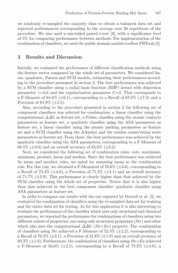
Prediction of Protein-Protein Binding Hot Spots 167
we randomly re-sampled the majority class to obtain a balanced data set andreported performances corresponding to the average over 20 repetitions of theprocedure. We also used a one-tailed paired t-test [3], with a significance levelof 5% for comparing performance between methods. For implementation of thecombination of classifiers, we used the public domain matlab toolbox PRTools [5].
3 Results and Discussion
Initially, we evaluated the performance of different classification methods usingthe feature vector composed by the whole set of parameters. We considered lin-ear, quadratic, Parzen and SVM models, estimating their performances accord-ing to the procedure presented in section 2. The best performance was achievedby a SVM classifier using a radial basis function (RBF) kernel with dispersionparameter γ=2.6 and the regularization parameter C=2. That corresponds toa F-Measure of 64.6% (±6.1), corresponding to a Recall of 67.6% (±7.3) and aPrecision of 61.9% (±5.5).
Also, according to the procedure presented in section 2 the following set ofcomponent classifiers was selected for combination: a linear classifier using thecomputational ΔΔG as feature set, a Fisher classifier using the atomic contactsparameters as feature set, a quadratic classifier using the ASA parameters asfeature set, a linear classifier using the atomic packing parameters as featureset and a SVM classifier using the AAindex and the residue conservation scoreparameters as feature set. From these, the best performance was achieved by thequadratic classifier using the ASA parameters, corresponding to a F-Measure of68.5% (±3.0) and an overall accuracy of 65.6% (±3.2).
Next, we considered the following set of combination rules: vote, maximum,minimum, product, mean and median. Since the best performance was achievedby mean and product rules, we opted for assuming mean as the combinationrule. For this rule, we obtained a F-Measured of 70.6% (±3.6), corresponding toa Recall of 72.4% (±4.6), a Precision of 71.3% (±2.1) and an overall accuracyof 71.7% (±3.9). This performance is clearly higher than that achieved by theSVM classifier using the whole set of properties. Notice that it is also higherthan that achieved by the best component classifier: quadratic classifier usingASA parameters as feature set.
In order to compare our results with the one reported by Darnell et al. [4], weevaluated the combination of classifiers using the re-sampled data set for trainingand the entire data set for testing. As for this application it is also interesting toevaluate the performance of the classifier which uses only structural and chemicalparameters, we reported the performance for combinations of classifiers using twodifferent subset of properties: one using only structural properties (Str) and otherwhich also uses the computational ΔΔG (Str+En) property. The combinationof classifiers using Str achieved a F-Measure of 52.4% (±2.2), corresponding toa Recall of 70.2% (±3.1), a Precision of 41.8% (±1.9) and an overall accuracy of69.3% (±1.6). Furthermore, the combination of classifiers using Str+En achieveda F-Measure of 56.6% (±2.5), corresponding to a Recall of 72.2% (±4.0), a
168 R.H. Higa and C.L. Tozzi
Precision of 46.6% (±2.0) and an overall accuracy of 73.4% (±1.5). By using at-test with significance level of 5%, the F-Measure achieved by Str+En is higherthan those reported by Darnell et al. [4].
4 Concluding Remarks
The prediction of protein-protein binding hot spot has been investigated bya strategy of combining classifiers and a set of structural, chemical and energybased properties. We report a performance of 56.6%, measured by the F-Measure,corresponding to a Recall of 72.2% and a Precision of 46.6%. By using a t-testwith significance level of 5%, this performance is higher than that reported byDarnell et al. [4] using the same data set.
References
1. Apweiler, R., Bairoch, A., Wu, C.H., et al.: UniProt: The Universal Protein Knowl-edgebase. Nucl. Acid. Res. 32, D115–D119 (2004)
2. Arkin, M.R., Wells, J.A.: Small-Molecule Inhibitors of Protein-Protein Interac-tions: Progressing Towards the Dream. Nature Reviews, Drug Discovery 3, 301–317(2004)
3. Bussab, W.O., Morettin, P.A.: Basic Statistics, 5th edn. Editora Saraiva, SaoPaulo, Brazil (2002) (in Portuguese)
4. Darnell, S.J., Page, D., Mitchell, J.C.: An Automated Decision-Tree Approach toPredicting Protein Interaction Hot Spots. Proteins 68, 813–823 (2007)
5. Duin, R.P.W., Juszczak, P., Paclik, P., et al.: PRTools4, a Matlab Toolbox forPattern Recognition, Delft University of Technology (2004)
6. Hagerty, C.G., Munchnik, I., Kulikowski, C.: Two Indices Can Approximate FourHundred and Two Amino Acid Properties. In: Proc. of 1999 IEEE Int. Simp. Intell.Control./Intell. Syst. and Semiotics, Cambridge, MA, pp. 365–369 (1999)
7. Kortemme, T., Baker, D.: A Simple Physical Model for Binding Energy Hot Spotsin Protein-Protein Complexes. Proc. Natl. Acad. Sci. USA 99, 14116–14121 (2002)
8. Liang, J., Edelsbrunner, H., Fu, P., Sudhakar, P.V., et al.: Analytical Shape Com-putation of Macromolecules: I. Molecular Area and Volume through Alpha Shape.Proteins 33, 1–17 (1998)
9. Mancini, A.L., Higa, R.H., Oliveira, A., et al.: STING Contacts: A Web-Basedapplication for Identification and Analysis of Amino Acid Contacts within ProteinStructure and Across Protein Interfaces. Bioinformatics 20(13), 2145–2147 (2004)
10. Moreira, I.S., Fernandes, P.A., Ramos, M.J.: Hot Spots - A Review of the Protein-Protein Interface Determinant Amino-Acid Residues. Proteins 68, 803–812 (2007)
11. Pupko, R., Bell, R.E., Mayrose, I., et al.: Rate4Site: An Algorithmic Tool for theIdentification of Functional Regions in Proteins by Surface Mapping of Evolution-ary Determinants Within Their Homologues. Bioinformatics 18(Supl.1), S71–S77(2002)
12. Webb, A.: Statistical Pattern Recognition. Wiley, Chichester (2002)
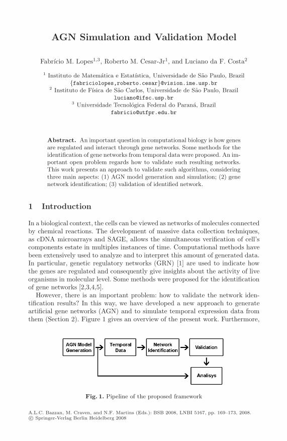
AGN Simulation and Validation Model
Fabrıcio M. Lopes1,3, Roberto M. Cesar-Jr1, and Luciano da F. Costa2
1 Instituto de Matematica e Estatıstica, Universidade de Sao Paulo, Brazil{fabriciolopes,roberto.cesar}@vision.ime.usp.br
2 Instituto de Fısica de Sao Carlos, Universidade de Sao Paulo, [email protected]
3 Universidade Tecnologica Federal do Parana, [email protected]
Abstract. An important question in computational biology is how genesare regulated and interact through gene networks. Some methods for theidentification of gene networks from temporal data were proposed. An im-portant open problem regards how to validate such resulting networks.This work presents an approach to validate such algorithms, consideringthree main aspects: (1) AGN model generation and simulation; (2) genenetwork identification; (3) validation of identified network.
1 Introduction
In a biological context, the cells can be viewed as networks of molecules connectedby chemical reactions. The development of massive data collection techniques,as cDNA microarrays and SAGE, allows the simultaneous verification of cell’scomponents estate in multiples instances of time. Computational methods havebeen extensively used to analyze and to interpret this amount of generated data.In particular, genetic regulatory networks (GRN) [1] are used to indicate howthe genes are regulated and consequently give insights about the activity of liveorganisms in molecular level. Some methods were proposed for the identificationof gene networks [2,3,4,5].
However, there is an important problem: how to validate the network iden-tification results? In this way, we have developed a new approach to generateartificial gene networks (AGN) and to simulate temporal expression data fromthem (Section 2). Figure 1 gives an overview of the present work. Furthermore,
Fig. 1. Pipeline of the proposed framework
A.L.C. Bazzan, M. Craven, and N.F. Martins (Eds.): BSB 2008, LNBI 5167, pp. 169–173, 2008.c© Springer-Verlag Berlin Heidelberg 2008

170 F.M. Lopes, R.M. Cesar-Jr, and L. da F. Costa
a network identification method [2] (Section 3) was incorporated, and the iden-tified networks are validated based on AGN model (Section 4). In Section 5, arepresented preliminary results. This paper is concluded in Section 6.
2 AGN Model Generation and Simulation
Two theoretical models of complex networks [6,7,8], corresponding to the scale-free Barabasi-Albert (BA) and the uniformly-random Erdos-Renyi (ER), havebeen considered in our network generation approach. More specifically, the gen-eration starts with a network size N (i.e. number of nodes) and a average degreek. The BA networks were grown starting with m0 nodes, to which additionalnodes with m = k edges each were successively attached preferentially to thedegree of the existing nodes. The ER structures were generated by implementingedges between every pair of nodes with fixed probability p. In order to ensuresimilar average degrees, we imposed the condition p = k
N−1 .Therefore, an AGN is formed by a set of N genes, g1, g2, ..., gN , which may
assume a value from a discrete set Y (in this work, Y = {0, 1}). The edges aredefined as a mapping function Ψ(gi) = {p1i, p2i, ..., pki}, in which pki (predictors)represents the genes that have input edges to gi (target). For each target it isbuilt a table containing all possible predictor’s combination values. For each gi
a value v ∈ Y is randomly defined. These rule tables define the simulation ofthe dynamical expression, i.e given the initial values of the N genes and thenumber of transitions T , the dynamics starts from t0 (initial values) and eachtarget’s state at ti 0 < i < T is obtained observing the predictors states atti−1 and its rule table. As a result, we have the simulated temporal data withT instants of time (transitions), which are used for the network identificationprocess presented in the following section.
3 Network Identification
The identification method used in this work is described in [2], in which genenetwork identification is modeled as a series of feature selection problems, onefor each gene. Therefore, the Sequential Forward Floating Selection (SFFS) [9]algorithm was performed for each target gene in order to select the SZ set thatminimizes the criterion function (mean conditional entropy) (1). The selectedfeatures are taken as predictor genes for each target, which are used to link thegenes and thus the identification of network topology.
E[H(Y |SZ)]=cP
i=1
H(Y |sZi)(oi+α)αc+T
, H(Y |SZ =sZi) = −1P
y=0
P (y|sZi) log P (y|sZi) (1)
where SZ is the set with one or more predictors, sZi is one instance of SZ andc = |Y ||SZ | is the possible number of instances of SZ . The term oi is the numberof occurrences of instance sZi in temporal data and α is the penalty weight forno observed instances (α = 1 in the present work).

AGN Simulation and Validation Model 171
4 Validation
Considering both models: BA and ER, the AGNs were represented in termsof their respective adjacency matrices K, such that each edge from node i tonode j implies K(j, i) = 1, with K(j, i) = 0 otherwise. In order to quantify thesimilarity between two given networks A (AGN) and B (identified network), weadopted the similarity measurements presented in [10], which are calculated asfollows:
g(A, B) =√
R1R0, R1 =b1
A1, R0 =
b0
A0(2)
We consider the geometrical average g(A, B) between the ratios of correct ones(R1) and correct zeros (R0), observing that matrix A contains A0 zeros and A1
ones, and matrix B contains b0 zeroes coinciding with the zeroes of A and b1
coinciding ones. Observe that both coincidences and differences are taken intoaccount by these indices, implying the maximum similarity to be obtained forindices values near 1.
5 Experimental Results
In all experiments, the two network architectures BA and ER with 100 nodeswere used. The average degree varied from 1 to 5 and the number of transitionsvaried from 10 to 250 in steps of 20.
Figure 2 presents the network identification results by increasing the numberof transitions. Clearly we can observe an improvement in the results using a largernumber of transitions. However, the experiments indicated that some temporalsignals do not present variations after fewer observations of time.
In order to avoid this effect, time signals were generated using from 1 to 9different initializations with random initial values, which were concatenated inone single temporal signal. Figure 3 presents the median results considering allvariations of transitions and average degrees. Based on our observations, an im-provement was confirmed by the results for increasing number of initializations,specially in BA-model (c) presenting excellent correct network recovery: 95%.
a) BA b) ER
Fig. 2. Network identification rate considering the increasing number of transitions

172 F.M. Lopes, R.M. Cesar-Jr, and L. da F. Costa
a) BA b) ER
Fig. 3. Network identification rate considering the number of initializations
6 Conclusion
The proposed framework is based on a AGN model that allows to simulate tem-poral expression data from it. The data was analyzed by a network identificationmethod and its results validated by the AGN model. The results indicate thatthe number of transitions is very important and that the use of concatenationsof temporal signals represents an important procedure to obtain better resultsfor the network identification, mainly because normally biological experimentsproduce replicas that can be used by computational methods.
The next stage of this work is to implement complex network measurements [8]and then to analyze network structures like hubs and communities. Other rel-evant improvement is to change the rule tables by joint probability functions,including some uncertainty in the creation of simulated data.
Acknowledgments
Luciano da F. Costa thanks CNPq (308231/03-1) and FAPESP (05/00587-5) forsponsorship. This work was supported by FAPESP, CNPq and CAPES.
References
1. Shmulevich, I., Dougherty, E.R.: Genomic Signal Processing, 1st edn. PrincetonUniversity Press, New Jersey (2007)
2. Barrera, J., Cesar Jr., R.M., Martins Jr., D.C., et al.: Constructing probabilisticgenetic networks of Plasmodium falciparum from dynamical expression signals ofthe intraerythrocytic development cycle. In: Methods of Microarray Data AnalysisV. Springer, Heidelberg (2006)
3. Liang, S., Fuhrman, S., Somogyi, R.: Reveal: a general reverse engineering algo-rithm for inference of genetic network architectures, pp. 18–29 (1998)
4. Shmulevich, I., et al.: Probabilistic boolean networks: a rule-based uncertaintymodel for gene regulatory networks. Bioinformatics 18(2), 261–274 (2002)

AGN Simulation and Validation Model 173
5. Mendes, P., Sha, W., Ye, K.: Artificial gene networks for objective comparison ofanalysis algorithms. Bioinformatics 19(Suppl. 2), 122ii–129 (2003)
6. Albert, R., Barabasi, A.L.: Statistical mechanics of complex networks. Rev. Mod.Phys. 74(1), 47–97 (2002)
7. Newman, M.E.J.: The structure and function of complex networks. SIAM Re-view 45(2), 167–256 (2003)
8. da F. Costa, L., Rodrigues, F.A., et al.: Characterization of complex networks: asurvey of measurements. Advances in Physics 56(1), 167–242 (2007)
9. Pudil, P., Novovicova, J., Kittler, J.: Floating search methods in feature selection.Pattern Recogn. Lett. 15(11), 1119–1125 (1994)
10. da F. Costa, L., et al.: Predicting the connectivity of primate cortical networks fromtopological and spatial node properties. BMC Systems Biology 1, 1–16 (2007)

A Practical Evaluation of BioProvider
(Extended Abstract)
Maira Ferreira de Noronha1, Sergio Lifschitz1, and Antonio Basilio de Miranda2
1 PUC-Rio Depto Informatica, Rio de Janeiro, Brazil{maira,sergio}@inf.puc-rio.br
2 FIOCRUZ, DBBM, Rio de Janeiro, [email protected]
Abstract. We present here an instantiation of BioProvider, a tool thatefficiently provides data for biological applications, tailored to the wayBLAST demands data. We briefly discuss some of the factors that mayinfluence data availability and performances.
1 Introduction
One of the most important tasks for the analysis of molecular biology datais sequence comparison. Biological applications such as BLAST [3] and Smith-Waterman [5] are the preferred and most popular tools for sequence comparison.This work evaluates a data management oriented tool aiming at delivering bio-logical data efficiently to multiple biological applications.
This tool, called BioProvider [4], is inspired on typical DBMS services. Onthe one hand, it allows ad-hoc management of memory buffers and, on the otherhand, the control of application’s process scheduling. All communications aredone through a device driver [2]. It is a non-intrusive approach that enablesusers to keep running their original applications while our tool provides theoptimized data access and availability.
This paper evaluates a specific instantiation of BioProvider for running withBLAST programs. The practical results obtained with BLAST indicate thatour database approach for developing BioProvider is well adapted for biologicalapplications and sequence data management.
2 BLAST Buffer Management and BioProvider
This work is mainly concerned with providing data access to biological appli-cations in a way similar to what database management systems (DBMS) dofor generic data and queries. The BioProvider proposal [4] introduces a generalapproach for dealing with biological data, particularly biological sequences. Inorder to evaluate our ideas, we will discuss here an instantiation of BioProviderthat works with BLAST - Basic Local Alignment Search Tool (e.g. [3]).
By taking the BLAST characteristics into account, our work in [1] suggestedan ad-hoc buffer management strategy for BLAST. The idea involves the usage of
A.L.C. Bazzan, M. Craven, and N.F. Martins (Eds.): BSB 2008, LNBI 5167, pp. 174–177, 2008.c© Springer-Verlag Berlin Heidelberg 2008
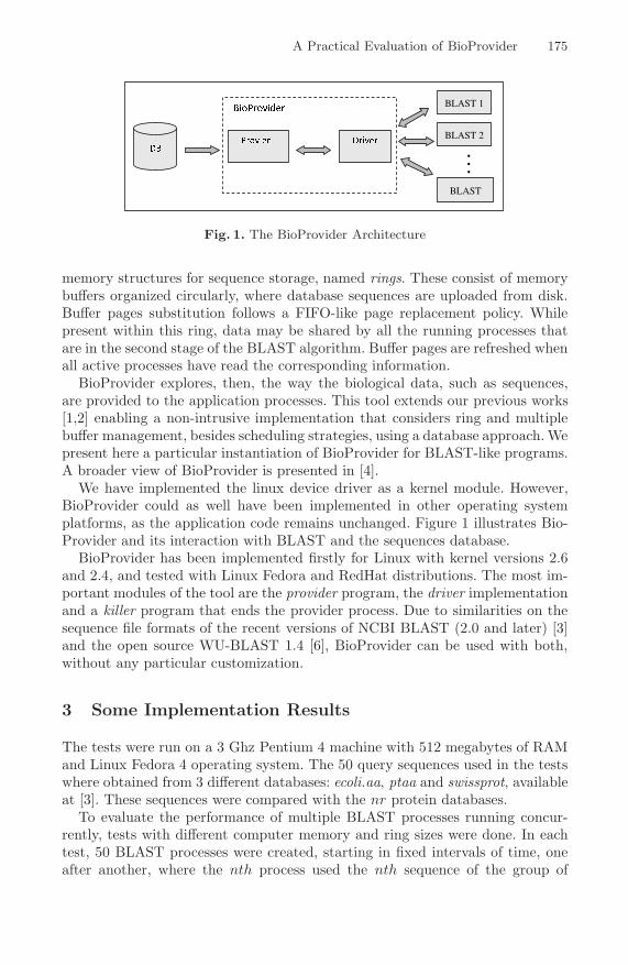
A Practical Evaluation of BioProvider 175
BLAST 2
BLAST 1
BLAST
DB .
.
.
BioProvider
Driver Provider
Fig. 1. The BioProvider Architecture
memory structures for sequence storage, named rings. These consist of memorybuffers organized circularly, where database sequences are uploaded from disk.Buffer pages substitution follows a FIFO-like page replacement policy. Whilepresent within this ring, data may be shared by all the running processes thatare in the second stage of the BLAST algorithm. Buffer pages are refreshed whenall active processes have read the corresponding information.
BioProvider explores, then, the way the biological data, such as sequences,are provided to the application processes. This tool extends our previous works[1,2] enabling a non-intrusive implementation that considers ring and multiplebuffer management, besides scheduling strategies, using a database approach. Wepresent here a particular instantiation of BioProvider for BLAST-like programs.A broader view of BioProvider is presented in [4].
We have implemented the linux device driver as a kernel module. However,BioProvider could as well have been implemented in other operating systemplatforms, as the application code remains unchanged. Figure 1 illustrates Bio-Provider and its interaction with BLAST and the sequences database.
BioProvider has been implemented firstly for Linux with kernel versions 2.6and 2.4, and tested with Linux Fedora and RedHat distributions. The most im-portant modules of the tool are the provider program, the driver implementationand a killer program that ends the provider process. Due to similarities on thesequence file formats of the recent versions of NCBI BLAST (2.0 and later) [3]and the open source WU-BLAST 1.4 [6], BioProvider can be used with both,without any particular customization.
3 Some Implementation Results
The tests were run on a 3 Ghz Pentium 4 machine with 512 megabytes of RAMand Linux Fedora 4 operating system. The 50 query sequences used in the testswhere obtained from 3 different databases: ecoli.aa, ptaa and swissprot, availableat [3]. These sequences were compared with the nr protein databases.
To evaluate the performance of multiple BLAST processes running concur-rently, tests with different computer memory and ring sizes were done. In eachtest, 50 BLAST processes were created, starting in fixed intervals of time, oneafter another, where the nth process used the nth sequence of the group of

176 M.F. de Noronha, S. Lifschitz, and A.B. de Miranda
N/D
4,59
2,15 2,48
2,02 1,69
N/D
3,81
1,42 1,43 1,01 0,75
-
1,0
2,0
3,0
4,0
5,0
6,0
7,0
8,0
9,0
10,0
128 256 512
Exe
cuti
on
Tim
e (h
ou
rs)
Memory Size (MB)
Total times without Bioprovider
Total times using BioProvider
Average times without Bioprovider
Average times using Bioprovider
Fig. 2. Memory Size Factor, Test 1
sequences. This was done in order to simulate an environment where, from timeto time, users run BLAST processes. The data analyzed in our tests were theaverage and total execution time of the BLAST processes.
In order to analyze the impact of the memory size in performances, testswere done varying the RAM memory available in the computer. The same testswere performed without BioProvider. However, when the RAM memory was 128megabytes, the tests without BioProvider could not finish after over 30 hoursof execution and we have canceled it. Figure 2 shows the test results comparingBLAST process performances with and without BioProvider.
Memory size was shown to be a very important factor in the performance ofBLAST processes, as the smaller the memory, the worst the performance. Onthe other hand, the processes were less influenced from memory size when Bio-Provider was used. Therefore, the smaller the memory, the bigger the advantageof BioProvider. Besides allowing the execution of BLAST processes in otherwiseforbidding situations, BioProvider reduced the total and average time of pro-cess execution in 56% and 73% respectively in a machine with 256 megabytes ofRAM memory, and 21% and 48% in a machine with 512 megabytes.
Tests were also performed to analyze the impact of the ring size in the overallperformance. The results obtained are depicted in Figure 3. It can be observedthat, as expected, process performance declines when the ring is too big sincememory shortage occurs for the running processes. At the same time, a smallloss of performance can be perceived when the ring size is too small. This canbe explained by the need of more ring updates for BLAST processes to continuereading. BioProvider reduced the total execution time of the processes between8% and 21%, and the average execution time between 28% and 48%.
We have studied many other parameters that include the query sequences,their similarity with the sequence databases, as well as their lengths. We haveanalyzed also the impact of the number of sequences per block and, consequently,the size of the blocks as well. Due to the lack of space, we refer the reader to [4]for a detailed evaluation on these and other factors.
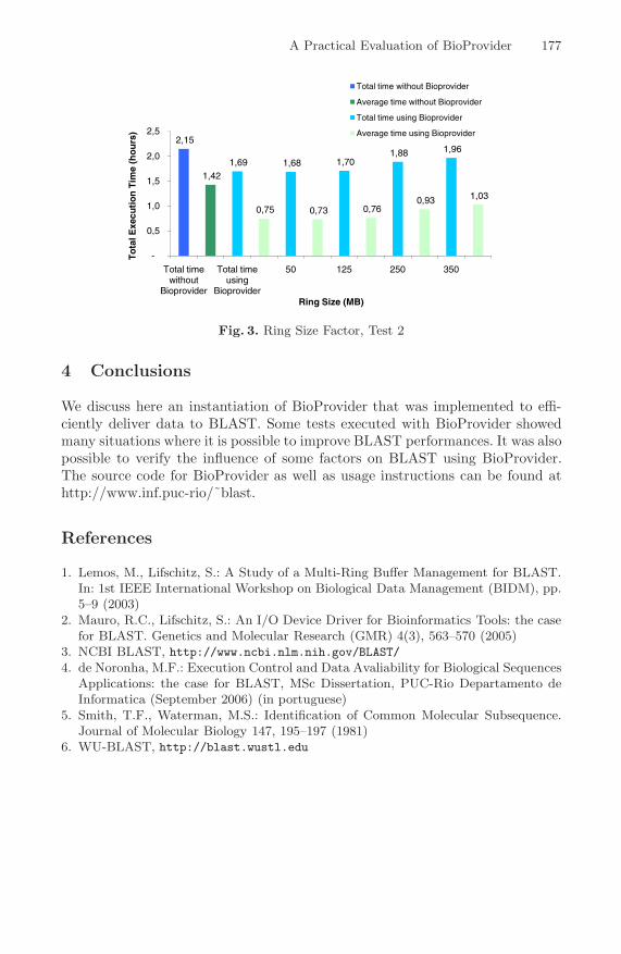
A Practical Evaluation of BioProvider 177
2,15
1,42 1,69
0,75
1,68
0,73
1,70
0,76
1,88
0,93
1,96
1,03
-
0,5
1,0
1,5
2,0
2,5
Total time without
Bioprovider
Total time using
Bioprovider
50 125 250 350
To
tal E
xecu
tio
n T
ime
(ho
urs
)
Ring Size (MB)
Total time without Bioprovider
Average time without Bioprovider
Total time using Bioprovider
Average time using Bioprovider
Fig. 3. Ring Size Factor, Test 2
4 Conclusions
We discuss here an instantiation of BioProvider that was implemented to effi-ciently deliver data to BLAST. Some tests executed with BioProvider showedmany situations where it is possible to improve BLAST performances. It was alsopossible to verify the influence of some factors on BLAST using BioProvider.The source code for BioProvider as well as usage instructions can be found athttp://www.inf.puc-rio/˜blast.
References
1. Lemos, M., Lifschitz, S.: A Study of a Multi-Ring Buffer Management for BLAST.In: 1st IEEE International Workshop on Biological Data Management (BIDM), pp.5–9 (2003)
2. Mauro, R.C., Lifschitz, S.: An I/O Device Driver for Bioinformatics Tools: the casefor BLAST. Genetics and Molecular Research (GMR) 4(3), 563–570 (2005)
3. NCBI BLAST, http://www.ncbi.nlm.nih.gov/BLAST/4. de Noronha, M.F.: Execution Control and Data Avaliability for Biological Sequences
Applications: the case for BLAST, MSc Dissertation, PUC-Rio Departamento deInformatica (September 2006) (in portuguese)
5. Smith, T.F., Waterman, M.S.: Identification of Common Molecular Subsequence.Journal of Molecular Biology 147, 195–197 (1981)
6. WU-BLAST, http://blast.wustl.edu
Evaluation of Models for the Recognition of
Hadwritten Digits in Medical Forms
Willian Zalewski1, Huei Diana Lee1, Adewole M.J.F. Caetano2,�,Ana C. Lorena2, Andre G. Maletzke3, Joao Jose Fagundes4,
Claudio Saddy4, Rodrigues Coy4, and Feng Chung Wu1
1 State University of West of Parana – Unioeste, Itaipu Technological Park, Brazil2 CMCC, ABC Federal University – UFABC, Brazil
3 ICMC, University of Sao Paulo – USP, Brazil4 FCM, State University of Campinas – Unicamp, Brazil
{willzal,hueidianalee}@gmail.com,{ana.lorena,adewole.caetano}@ufabc.edu.br
Abstract. Medicine has benefited widely from the use of computationaltechniques, which are often employed in the analysis of data generatedin medical clinics. Among the computational techniques used in theseanalyses are those from Knowledge Discovery in Databases (KDD). Inorder to apply KDD techniques in the analysis of clinical data, it is oftennecessary to map them into an adequate structured format. This paperpresents an extension in a methodology to map medical forms into struc-tured datasets, in which a sub-system for handwritten digit recognitionis added to the overall mapping system.
Keywords: Machine learning, digit recognition, medical forms.
1 Introduction
In Medicine, data are often disposed in medical reports and printed forms con-taining information like the patient’s history and symptoms, which difficult a di-rect analysis by computational algorithms. There are several reasons why thesedata are unavailable in an adequate format, among which are the inexistenceof computers in medical ambulatories, the common sense in Medicine that theuse of printed documents makes the relationship with the patient less imper-sonal and the necessity to maintain printed records. In previous work, a newmethodology for mapping medical forms into the attribute-value representationwas proposed and successfully employed in a medical case study [1].
This work presents an extension to the proposed methodology, where classifi-cation models for handwritten digit recognition are added to the overall mappingsystem.
� Financial support of PDTA-PTI/BR.
A.L.C. Bazzan, M. Craven, and N.F. Martins (Eds.): BSB 2008, LNBI 5167, pp. 178–181, 2008.c© Springer-Verlag Berlin Heidelberg 2008
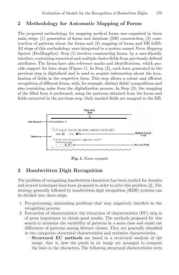
Evaluation of Models for the Recognition of Hadwritten Digits 179
2 Methodology for Automatic Mapping of Forms
The proposed methodology for mapping medical forms was organized in threemain steps: (1) generation of forms and database (DB) construction, (2) cons-truction of patterns about the forms and (3) mapping of forms and DB fulfill.All steps of this methodology were integrated to a system named Form MappingSystem (ForMappSys). Step (1) involves constructing forms, by a user-friendlyinterface, containing numerical and multiple choice fields from previously definedattributes. The forms have also reference marks and identifications, which pro-vide support for later steps (Figure 1). In Step (2), each form generated in theprevious step is digitalized and is used to acquire information about the loca-lization of fields in the respective form. This step allows a robust and efficientrecognition of different forms, with, for example, distinct fields’ compositions andalso containing noise from the digitalization process. In Step (3), the mappingof the filled form is performed, using the patterns obtained from the forms andfields extracted in the previous step. Only marked fields are mapped to the DB.
Fig. 1. Form example
3 Handwritten Digit Recognition
The problem of recognizing handwritten characters has been studied for decadesand several techniques have been proposed in order to solve this problem [2]. Thestrategy generally followed by handwritten digit recognition (HDR) systems canbe divided into three steps:
1. Pre-processing: minimizing problems that may negatively interfere in therecognition process;
2. Extraction of characteristics: the extraction of characteristics (EC) step isof great importance to obtain good results. The methods proposed for thissearch to minimize the variability of patterns in a same class and stand outdifferences of patterns among distinct classes. They are generally classifiedin two categories: structural characteristics and statistics characteristics.– Structural EC methods are based in a structural analysis of the
image, that is, how the pixels in an image are arranged to composethe lines in the characters. The following structural characteristics were
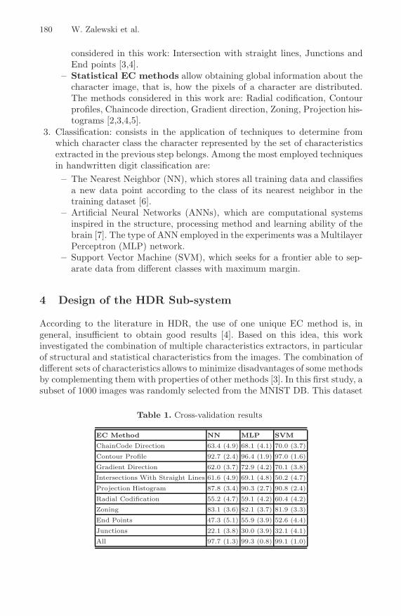
180 W. Zalewski et al.
considered in this work: Intersection with straight lines, Junctions andEnd points [3,4].
– Statistical EC methods allow obtaining global information about thecharacter image, that is, how the pixels of a character are distributed.The methods considered in this work are: Radial codification, Contourprofiles, Chaincode direction, Gradient direction, Zoning, Projection his-tograms [2,3,4,5].
3. Classification: consists in the application of techniques to determine fromwhich character class the character represented by the set of characteristicsextracted in the previous step belongs. Among the most employed techniquesin handwritten digit classification are:– The Nearest Neighbor (NN), which stores all training data and classifies
a new data point according to the class of its nearest neighbor in thetraining dataset [6].
– Artificial Neural Networks (ANNs), which are computational systemsinspired in the structure, processing method and learning ability of thebrain [7]. The type of ANN employed in the experiments was a MultilayerPerceptron (MLP) network.
– Support Vector Machine (SVM), which seeks for a frontier able to sep-arate data from different classes with maximum margin.
4 Design of the HDR Sub-system
According to the literature in HDR, the use of one unique EC method is, ingeneral, insufficient to obtain good results [4]. Based on this idea, this workinvestigated the combination of multiple characteristics extractors, in particularof structural and statistical characteristics from the images. The combination ofdifferent sets of characteristics allows to minimize disadvantages of some methodsby complementing them with properties of other methods [3]. In this first study, asubset of 1000 images was randomly selected from the MNIST DB. This dataset
Table 1. Cross-validation results
EC Method NN MLP SVM
ChainCode Direction 63.4 (4.9) 68.1 (4.1) 70.0 (3.7)
Contour Profile 92.7 (2.4) 96.4 (1.9) 97.0 (1.6)
Gradient Direction 62.0 (3.7) 72.9 (4.2) 70.1 (3.8)
Intersections With Straight Lines 61.6 (4.9) 69.1 (4.8) 50.2 (4.7)
Projection Histogram 87.8 (3.4) 90.3 (2.7) 90.8 (2.4)
Radial Codification 55.2 (4.7) 59.1 (4.2) 60.4 (4.2)
Zoning 83.1 (3.6) 82.1 (3.7) 81.9 (3.3)
End Points 47.3 (5.1) 55.9 (3.9) 52.6 (4.4)
Junctions 22.1 (3.8) 30.0 (3.9) 32.1 (4.1)
All 97.7 (1.3) 99.3 (0.8) 99.1 (1.0)

Evaluation of Models for the Recognition of Hadwritten Digits 181
was further evaluated with the 10-fold cross-validation methodology. Table 1presents the accuracy results and Standard deviation rates achieved in this firstset of experiments. Based in the results, the MLP technique was chosen forbuilding the final classification model of the HDR sub-system.
5 Case Study
A model form was built using the ForMappSys system. This form is composed offive multiple choice questions and four questions with numerical answers. Fiftycopies of the model form were made, filled ad libitum using a standard black penby ten collaborators.
Considering all forms, only one of the 250 multiple choice questions was notcorrectly mapped by ForMappSys system. Herewith, it is possible to evidence a99.6% of accuracy in mapping multiple choice fields. For the 504 digits manuallywritten in the forms, the accuracy of classification was of 96.23%.
6 Conclusion and Future Work
Specialists of the domain consider the results promising. The analysis of theresults showed that a large part of the filled digits in the forms were correctlyclassified. Future work includes selecting relevant attributes from the digits’ char-acteristics and combining classifiers to increase the reliability of the predictions.
References
1. Maletzke, A.G., Lee, H.D., Zalewski, W., Edson, R.F.V., Matsubara, T., Coy,C.S.R., Fagundes, J.J., Goes, J.R.N., Chung, W.F.: Mapeamento de informacoesmedicas descritas em formularios para bases de dados estruturadas [in portuguese],Brasil, pp. 1–10 (2007)
2. Trier, O.D., Jain, A.K., Taxt, T.: Feature extraction methods for character recog-nition - a survey. Pattern Recognition 29, 641–662 (1996)
3. Heutte, L., Paquet, T., Moreau, J.-V., Lecourtier, Y., Olivier, C.: A structural/statistical feature based vector for handwritten character recognition. PatternRecognition Letters 19, 629–641 (1998)
4. Arica, N., Yarman-Vural, F.: An overview of character recognition focused on off-line handwriting. IEEE Trans. Syst. Man and Cybern. Part C: Appl. and Rev. 31,216–233 (2001)
5. Wang, X., Xie, K.: A novel direction chain code-based image retrieval. In: Proc. 4thInt. Conf. on Computer and Information Technology, pp. 190–193 (2004)
6. Lee, Y.: Handwritten digit recognition using k- nearest neighbor, radial-basis func-tions, and back-propagation neural networks. Neural Comp. 3(3), 440–449 (1991)
7. Haykin, S.: Neural Networks - A Compreensive Foundation. Prentice-Hall, Engle-wood Cliffs (1999)

Author Index
A. Hausen, Rodrigo de 79Alves, Roberto T. 1Andrade-Navarro, Miguel 92
Barros, Matheus B.S. 13Borges, Carlos Cristiano H. 140Breda, Ardala 47Brıgido, Marcelo M. 127Bugalho, Miguel M.F. 23
Caetano, Adewole M.J.F. 178Carvalho, Andre C.P.L.F. 35Castro-e-Silva, Alcides 161Cesar-Jr., Roberto M. 169Chiu, David K.Y. 57Costa, Eduardo P. 35Coy, Rodrigues 178
Delgado, Myriam R. 1Dias, Zanoni 115Dorn, Marcio 47
F. Costa, Luciano da 169Fagundes, Joao Jose 178Faria, Luerbio 79Figueiredo, Celina M.H. de 79Fonseca, Lucas O. da 127Freitas, Alex A. 1, 35
Gadish, Moshe A. 57Gomes, Diego E.B. 68Guerra-Sa, Renata 161
Higa, Roberto Hiroshi 165
Kowada, Luis Antonio B. 79
Lee, Huei Diana 178Li, Shenggang 92Lifschitz, Sergio 174Lins, Roberto D. 68L. Martins, Simone de 13Lopes, Fabrıcio M. 169Lorena, Ana C. 35, 178
Machado, Karina S. 104Machado, Romuel F. 161Maletzke, Andre G. 178Mira, Cleber V.G. 115Miranda, Antonio Basilio de 174
Norberto de Souza, Osmar 47, 104Noronha, Maira Ferreira de 174
Oliveira, Arlindo L. 23
Pascutti, Pedro G. 68Pinto, Guilherme A. 115Plastino, Alexandre 13
Ralha, Celia Ghedini 127Ruiz, Duncan D. 104
Saddy, Claudio 178Sankoff, David 92, 152Santos, Hederson P. 115Schneider, Hugo W. 127Schroeder, Evelyn K. 104Silva, Joao C.P. da 140Soares, Thereza A. 68Straatsma, Tjerk P. 68
Tozzi, Clesio Luis 165
Vasconcelos, Ana Tereza R. 140
Walter, Maria Emilia M.T. 115, 127Wanderley, Maria Fernanda B. 140Wanner, Elizabeth F. 161Weber, Gerald 161Wink, Ana 104Wu, Feng Chung 178
Xu, Ximing 152
Zalewski, Willian 178
Related Documents