Identifying, visualizing and quantifying process ...publications.lib.chalmers.se/records/fulltext/43071.pdf · Identifying, visualizing and quantifying process disturbances at SSAB

Identifying, visualizing and quantifying process disturbances at SSAB Oxelösund using multivariate modelling

Diploma Thesis in the Biotechnology Engineering Programme

HENRIK RÅDBERG

Department of Chemical Reaction Engineering Division of Chemistry and Biotechnology CHALMERS UNIVERSITY OF TECHNOLOGY Göteborg, Sweden, 2007

This report is a part of a research project supervised by IVL Swedish Environmental Research Institute Ltd.


© Henrik Rådberg, 2007

Department of Chemical Reaction Engineering Chalmers University of Technology SE–412 96 Göteborg, Sweden

Department of Chemical Reaction Engineering Göteborg, 2007

Cover: Crude iron discharge from blast furnace, SSAB Tunnplåt AB, Luleå Photo: Stig-Göran Nilsson (2002) The illustration shows principal components describing variation in a data set

3

Abstract


Henrik Rådberg Department of Chemical Reaction Engineering Chalmers University of Technology Modern process lines give rise to huge amounts of data which are stored in databases. Mul-tivariate analysis comprises useful tools to grasp useful information from the datasets. In the present study principal component analysis (PCA), projection to latent structures (PLS) and hierarchical PCA has been used to create models of five process steps at a Swed-ish steelworks. The focus has been to identify and explain relations to quality problems in each step, both within the step itself, but also from upstream processes using hierarchical PCA. The five process steps that have been modelled are the blast furnace, desulphurization in the torpedo car, basic oxygen steelmaking in the LD–LBE-converter, secondary steelmak-ing in ladle and ladle furnace and, finally, continuous casting of slabs. Among the results achieved it is found that:

� PLS prediction of crude iron analysis from blast furnace discharge has been made with a fraction of explained variance for external validation (Q2

PS) above 20% for P, Cr, Cu, Ti, CaO, SiO2, MgO and basicity. The data resolution was relatively low.

� Hierarchical modelling revealed correlations between the process steps, e.g. that

LD-converter treatments registered as severe slopping heats have a titanium con-tent in the incoming crude iron that is higher than average.

� Heats with too high phosphorous content after LD-treatment can be identified as

having low silicon content in the crude iron, which makes it impossible to create the necessary slag amount for desired phosphorous cleaning effect.

� High sulphur content in the torpedo car demands a long treatment time. If the sili-

con content is low in such a batch, there is an evident risk that it will not have high enough temperature in the secondary steelmaking.

� Capturing reasons for quality problems during casting is difficult due to the low

variation in data. The main variations exist between the steel qualities. However, the importance of casting properties such as oscillations for visual quality of the slabs, and temperature and steel analysis for slab inner quality have been recog-nized.

Keywords: Multivariate analysis; PCA; PLS; hierarchical modelling; process modelling; blast furnace; steelworks

4

Sammanfattning

Moderna processindustrier ger upphov till stora mängder data som sparas i databaser. För att analysera dessa datauppsättningar och få ut användbar information används ofta statis-tiska verktyg i form av multivariata metoder såsom principalkomponent analys (PCA) och projektion till latenta strukturer (PLS). PCA används för klassificering och för att skaffa sig en överblick över de observationer (objekt) som finns i datauppsättningen medan PLS an-vänds för prediktion av en eller flera intressanta responser (Y-variabler). I detta arbete PCA och PLS använts för att modellera fem processteg på SSAB Oxelösunds stålverk. Fo-kus har legat på att identifiera och förklara samband mellan kvalitetsproblem i varje pro-cessteg. Sambanden har sökts såväl inom processteget som i tidigare processer genom an-vänding av hierarkisk modellering. De fem processteg som undersökts är masugn, avsvavling i torpeder, färskning i LD–LBE-konverter, skänkmetallurgi och stränggjutning. Bland erhållna resultat märks följande:

� PLS-prediktion av råjärnsanalyser från masugnstappningar har gett förklarings-grader på över 20% vid extern validering (Q2

PS) för följande ämnen: P, Cr, Cu, Ti, CaO, SiO2, MgO samt basicitet.

� Hierarkisk modellering har påvisat samband mellan processteg, exempelvis att

LD-charger med stora utkok haft högre titanhalt i råjärnet än medelvärdet av alla observationer.

� Charger med för hög fosforhalt efter färskning uppvisar samband med låg kiselhalt

i det inkommande råjärnet. Den låga kiselhalten förhindrar att tillräckligt mycket slagg kan bildas vilket hämmar fosfosreningen.

� Hög svavelhalt i råjärnet kräver långa behandlingstider i avsvavlingssteget. Om

dessutom kiselhalten är låg är det stor risk att chargen hamnar lägre i temperatur än gränsvärdet vid skänkbehandlingen tillåter.

� Modellering av kvalitetsproblem vid stränggjutningen har försvårats av låg varia-

tion i datauppsättningen eftersom de främsta variationerna återfinns mellan olika stålkvaliteter. Samband mellan kokillens oscillering och stålämnets ytkvalitet har dock kunnat fastställas, liksom inverkan av temperatur och stålsammansättning i gjutlådan på stålämnets inre kvalitet.

5

Contents

Abstract 3

Sammanfattning 4

Contents 5

1. Objectives and scope 7

1.1. Objectives 7

1.2. Scope 7

2. Theoretical background 8

2.1. Multivariate statistical methods 8

2.1.1. Principal component analysis (PCA) 9

2.1.2. Projection to latent structures (PLS) 13

2.1.3. Hierarchical modelling 16

2.2. Steelmaking 16

2.2.1. Overview of the process 17

2.2.2. Thermodynamics and kinetics 18

2.2.3. Crude iron production: Blast furnace 19

2.2.4. Desulphurization: Torpedo car 21

2.2.5. Basic oxygen steelmaking: LD–LBE-converter 21

2.2.6. Secondary steelmaking: TN-station and ladle furnace 22

2.2.7. Continuous casting 23

2.2.8. Challenges in the production line 24

2.3. Previous studies of steelworks using multivariate methods 25

3. Data treatment and modelling 27

3.1. Data pretreatment 27

3.1.1. Data extraction and structure 27

3.1.2. Variable selection 28

3.1.3. Block construction 29

3.2. Modelling 29

3.2.1. Block modelling 29

3.2.2. Hierarchical modelling 31

4. Results 32

4.1. Block modelling 32

4.1.1. Blast furnace (BF) 32

6

4.1.2. Desulphurization (TP) 34

4.1.3. Basic oxygen furnace (LD) 35

4.1.4. Secondary steelmaking (SS) 36

4.1.5. Continuous casting (CC) 37

4.2. Hierarchical modelling 39

4.2.1. Slopping 40

4.2.2. Analysis misses 40

4.2.3. Temperature misses 40

4.2.4. Slab quality 41

5. Discussion and conclusions 42

5.1. Blast furnace modelling 42

5.2. Desulphurization and LD-treatment 42

5.3. Secondary steelmaking 43

5.4. Continuous casting 43

6. Proposals 45

Acknowledgements 46

References 47

Appendix A: Engelsk–svensk ordlista 49

Appendix B: Variable list 50

Primary observation identification 50

Observation labels 50

Variables in the blast furnace block 51

Variables in the desulphurization block 52

Variables in the basic oxygen furnace block 53

Variables in the secondary steelmaking block 54

Variables in the continuous casting block 56

7

1. Objectives and scope

The amount of process data collected at modern process facility makes it possible to use multivariate techniques to gather useful information about the process in a variety of ways, for example:

� Classify a process state as belonging to normal operation or not. � Reveal underlying explanations to known disturbances. � Detect unknown disturbances and suggest causalities. � Predict important quantities or qualities.

It is however important to have an idea of what phenomena that may be present and possi-ble to study before starting to collect and treat data. This study is performed as a part of a research project supervised by IVL Swedish Environmental Research Institute, and the objectives and scope are described in subsequent sections.

1.1. Objectives Data from both ironworks and steelworks are included in the study and divided into blocks which correspond to the process steps. The main objective is to identify, visualize and quan-tify process disturbances at the plant by modelling each block and also connect data from the iron- and steelworks using hierarchical modelling. The top-level model is based on the models for each of the data blocks. The process disturbances may cause faults such as non-satisfactory and varying crude iron composition, slopping during basic oxygen steelmaking, failure reaching the liquid steel product specification and quality problems while casting. The aim is to describe these dis-turbances well enough for actions to be taken.

1.2. Scope The process equipment at different steelworks may vary from each other, therefore the theoretical description of steel production as well as literature and papers studied are mostly for process lines similar to the one at SSAB Oxelösund. The term process line is here used for the five steps crude iron production, desulphurization, basic oxygen steelmak-

ing, secondary steelmaking and continuous casting. SSAB Oxelösund produces a variety of steel qualities. Internally these are named T-sorts, each having its specific process route and quality specification. Three T-sorts have been included in the data studied (in this study called T1, T2 and T3), constituting common products with challenges meeting quality targets, especially in the casting step. Although the T-sorts do not have exactly the same properties, they are included in the same dataset for comparison. A wide range of phenomena and correlations in the process line may be studied using mul-tivariate techniques, but focus in this study is to identifying factors affecting the quality tar-gets in each process step and thereafter to quantify their influence. The quality targets are illustrated in figure 15 in section 3.1.3.

8

2. Theoretical background

In this chapter the tools used for data analysis are presented together with a description of the steelmaking process in general and the SSAB Oxelösund steelworks in particular.

2.1. Multivariate statistical methods The aim for multivariate analysis is to present useful information from large amounts of data that may be difficult to grasp in more traditional ways. The methods used in this study are based on the idea of latent structures available in the original data. The concept can be illustrated by a comparison with the human colour vision as is done by Martens and Naes (1991), see figure 1. The sunlight consists of several wavelengths, of which the ones between 400 and 700 nm are what we call visible light. If these wavelengths encounter a red cloth, the “red” (600–700 nm) are being reflected and eventually registered by the human eye, which registers the information as the three quantities red/green, yel-low/blue and light/dark and passes this information on through nerve cells. Even though the incoming light consists of tens or more wavelengths, three variables (together with in-formation about the light source’s original spectra, which the brain is aware of) is enough to produce meaningful colour information. These three pairs are in this case the latent vari-ables that the incoming spectra are compressed into.

Figure 1. Colour vision as an illustration of latent variable construction. The sunlight consists of hundreds of wave-lengths. The red wavelengths are reflected by the red cloth and captured by three pigments in the eye. Three nerve

signals pass on the wavelength information to the brain which calculates the three-dimensional colour space.

In this study two latent variable methods have been used to model the different process steps at SSAB Oxelösund; principal component analysis and projection to latent structures (also known as partial least squares). A common thing with these methods is that they pro-duce models that are more compact and statistically stable than the data matrix X (Mar-tens & Martens 2001). In addition, results from the individual models have been imple-mented in a top model by hierarchical methods, described in subsection 2.1.3.

9

2.1.1. Principal component analysis (PCA)

Several objectives may be the background for using principal component analysis (PCA). Wold et al (1987) lists some of them in their PCA tutorial: simplification, data reduction, modelling, outlier detection, variable selection, classification, unmixing and prediction. Using PCA to construct the latent variables out of a data matrix XX is basically a task of least squares calculation. The different observations made are stored as rows (often called objects) in X and the variables measured constitute the columns. The main patterns in the data in X are captured in a few principal components (PCs), stored in the small matrices T and P 0. The column vectors in T carry information about patterns in the observations while the rows in P 0 are related to the variables and their individual contributions to the principal component. Plotting is usually a good tool to visualize the information achieved in the PCs.

2

6

4

x11 ¢ ¢ ¢ x1K

.... . .

...xN1 ¢ ¢ ¢ xNK

3

7

5=

2

6

4

t11

...tN1

3

7

5

2

6

4

p11

...pK1

3

7

5

0

+ ¢ ¢ ¢ +

2

6

4

t1A

...tNA

3

7

5

2

6

4

p1A

...pKA

3

7

5

0

+

2

6

4

e11 ¢ ¢ ¢ e1K

.... . .

...eN1 ¢ ¢ ¢ eNK

3

7

5

2

6

4

x11 ¢ ¢ ¢ x1K

.... . .

...xN1 ¢ ¢ ¢ xNK

3

7

5=

2

6

4

t11

...tN1

3

7

5

2

6

4

p11

...pK1

3

7

5

0

+ ¢ ¢ ¢ +

2

6

4

t1A

...tNA

3

7

5

2

6

4

p1A

...pKA

3

7

5

0

+

2

6

4

e11 ¢ ¢ ¢ e1K

.... . .

...eN1 ¢ ¢ ¢ eNK

3

7

5

Figure 2. Matrix notation for a schematic extraction of data matrix X into A principal components and residual matrix E.

The PC’s can be calculated in a iterative manner using the NIPALS (non-linear iterative partial least squares) algorithm. The vector ti (i = 1:::Ai = 1:::A, where A is the number of compo-nents calculated) is called the score vector and pipi is denoted loading vector. Geometrically the principal component may be interpreted as the straight line best fitted to the N data points in a space spanned by K variables.

Figure 3. The score tijtij is the orthogonal projection of the jjth observation onto the axis of the iith principal component. The loading vector pipi contains the direction coefficients for the PC.

The slope of the PC reveals the direction of maximal variance. The following components will be orthogonal to the previous ones, and by calculating A = min(K;N)A = min(K;N) components a whole new set of axes are constructed, i.e. a coordinate system transformation has been made. However, when using PCA in studies like this, there is no meaning in taking too many components since the observations and variables contain noise. Meaningful informa-tion is only available in the first few components and using too many PC’s would only spoil the opportunity to classify or predict future observations.

10

Data pretreatment Before the PCA is performed on the data matrix XX it may be necessary to do some trans-formations, centring and scaling of data. These three steps are not performed by routine but depend on how input data looks. Transformations may be used to correct for nonlinearities in original data. A common transformation is to take the logarithm of the XX-values, but there is a lot of various special-ized methods available. If different transformations are applied to the variables there is a risk for introducing a shear between the correlation matrix for XX and the one for the trans-formed data set (Wold et al 1987). Centring around each variable’s mean is used to achieve more stable computations. Since PCA is used to model the variation between the objects, centring will not influence the in-terpretation (Martens & Martens 2001). The relation between original data and the princi-pal components may then be written as X = 1¹x + TP 0 + EX = 1¹x + TP 0 + E , where 11 is a K £ 1K £ 1 column vec-tor only containing ones. Scaling is used to compensate that some variables may have larger absolute values than others, thereby giving each variable possibility to contribute equally to the PC’s. Usually scaling is performed by dividing each value with the standard deviation of the respective variable. In some cases scaling is not suggested, e.g. when modelling absorbance data the variables (wavelengths) are all of the same kind and scaling would have severe effect on the loadings pp calculated. Another pretreatment operation may be to create new variables, e.g. differences or ratios, calculated from the variables already present. Also, handling of missing data must be taken care of since all process data is not registered for all times. This may for example be due to transmission failures between sensor and database. In the present study, centring, scaling and creation of new variables have been used but no transformations. Missing data has been handled by an algorithm which is a part of the soft-ware used for modelling1.

Model validation When the model has been calculated it is important interpret it and to perform a proper diagnose where its accuracy and other quality aspects are validated. In order to do that, several statistical tools and useful plots can be calculated and studied. A first overview normally includes checking the amount of explained variance R2R2 and the amount of vari-ance that the model is able to predict (often denoted Q2Q2 or R2

predictionR2prediction). These two proper-

ties vary between 0 and 1 where unity indicates a good performance. They are calculated as follows:

R2 =SSR

SST

= 1¡SSE

SST

R2 =SSR

SST

= 1¡SSE

SST where SSRSSR is the explained sum of squares, SSTSST is the total sum of squares and SSESSE is the residual sum of squares. If the degrees of freedom are accounted for, the so called adjusted R2R2 can be calculated:

1 Simca-P+ 11.5 from Umetrics AB, Umeå, Sweden.

11

R2adj = 1

SSE

K¡A¡1SST

K¡1

= 1¡ (1¡R2)K ¡ 1

K ¡A¡ 1R2

adj = 1SSE

K¡A¡1SST

K¡1

= 1¡ (1¡R2)K ¡ 1

K ¡A¡ 1 where AA is the number of components and KK is the number of variables (if the number of observations, NN , are less than KK then NN should be used instead of KK). The R2

adjR2adj is used due

to the fact that R2R2 increases with every new component calculated, even if it does not model any important variance. R2

adjR2adj is able to compensate for the fact that a new compo-

nent has been calculated and will only increase if more variance than would be expected from random noise is explained (Montgomery 2001).

Q2 = 1¡PRESS

SSE

Q2 = 1¡PRESS

SSE where SSESSE is the residual sum of squares of the previous component (i.e. in correspon-dence with the amount of variance remaining to be explained) and PRESSPRESS is the predic-tion error sum of squares which is calculated as the sum of squares of the difference be-tween real XX-values and predicted ones:

PRESS =

NX

i=1

KX

j=1

(xij ¡ xij)2PRESS =

NX

i=1

KX

j=1

(xij ¡ xij)2

The predicted value xijxij is achieved by cross validation (CV) which also is a tool for deter-mining the number of significant components in the model. It can be done in several ways but is based on the idea of excluding some of the data, calculating a new model, use that model to predict the excluded values and then comparing the excluded and compared val-ues when all data have been excluded one (and only one) time. In the software Simca-P+ used for modelling in this study, observations are first excluded for loadings to be calcu-lated, then variables are excluded and scores calculated. The ratio PRESS=SSEPRESS=SSE is then used to determine if the component calculated is significant – a ratio smaller than unity in-dicates that the predictive ability has increased with the last component (Montgomery 2001). Q2 may be calculated for a component, a variable in a component (Q2

var) or summed for all components, denoted Q2

acc. Depending on whether trends in the data exist or not, the way the cross validation blocks are chosen is of importance for the calculation of Q2. The relevance of the variables is for example determined by looking at the amount of ex-plained variance. A measure for that is the modelling power, MpowMpow, where the residual standard deviation for variable k is related to the initial standard deviation for the variable (Umetrics 2002):

Mpowk = 1¡¾k

¾k0Mpowk = 1¡

¾k

¾k0 Plotting MpowMpow for all variables enables good comparison of variable relevance. Excluding variables is however generally not recommended since removing the variable may seem to improve model properties but in reality that is not always true. Also apparently non-significant variables will contribute to the observations residuals or distance to model (DmodXDmodX, described in next subsection) (Wold 1987).

12

Plots and interpretation The first principal components calculated reveal most of the information that can be read-ily interpreted. A first look at the data will therefore be to plot the scores and loadings, see figure 4 (a, b, c).

-6

-4

-2

0

2

4

6

8

10

12

-12 -11 -10 -9 -8 -7 -6 -5 -4 -3 -2 -1 0 1 2 3 4 5 6 7 8 9

t[2

]

t[1]

SS02.M3 (PCA-X), T-sort T1t[Comp. 1]/t[Comp. 2]

R2X[1] = 0.0744934 R2X[2] = 0.0537219 Ellipse: Hotelling T2 (0.95)

SIMCA-P+ 11.5 - 2007-05-23 14:35:05

-0.1

0.0

0.1

0.2

-0.1 0.0 0.1 0.2

p[2

]

p[1]

SS02.M3 (PCA-X), T-sort T1p[Comp. 1]/p[Comp. 2]Colored according to model terms

R2X[1] = 0.0744934 R2X[2] = 0.0537219

EBTBGA SANTEBTBLTITOT

EBTGA SMGD

EBTTLTR1

EBTTLTR2

EBTLE5018

EBTLE5035EBTLE5230

EBTLE5303

EBTLE5499

EBTXLTS

EBTXTESL

EBTXTTS

EBTSTTV

EBVHBHTEBVEANT

EBV ETOTI

EBV HKWT

EBVHKWTOT

EBVGBTOTI

EBVHSB01

EBV HSB02

EBV HSB03EBVHSB04

EBVHSB05

EBV FSTOTI

EBVA CBEH

EBV HVLP1EBV HV101

EBVHA NGEBVHTEM1

EBVHSTV

EBSXNTSEBSULGN5018

EBSULGN5021

EBSULGN5030

EBSULGN5036

EBSULGN5045

EBSULGN5063

EBSULGN5121 EBSULGN5218

EBSULGN5232

EBSULGN5236

EBSULGN5303

EBSULGN5401

EBSULGN5404

EBSULGN5499

EBSULGN6605EBSULGN6610

EBCHNST

EBV HKRNS

EBSXLTS

KTMA TT234KTTRAFF234

KTMA TT236

KTTRAFF236

KTMATT321

KTTRAFF321

KTMATT341_2

KTTRA FF341_2

SIMCA-P+ 11.5 - 2007-05-23 14:36:21

-0.2

-0.1

-0.0

0.1

0.2

0.3

0.4

EB

TB

GA

SA

NT

EB

TB

LT

ITO

TE

BT

GA

SM

GD

EB

TT

LT

R1

EB

TT

LT

R2

EB

TL

E5

01

8E

BT

LE

50

35

EB

TL

E5

23

0E

BT

LE

53

03

EB

TL

E5

49

9E

BT

XL

TS

EB

TX

TE

SL

EB

TX

TT

SE

BT

ST

TV

EB

VH

BH

TE

BV

EA

NT

EB

VE

TO

TI

EB

VH

KW

TE

BV

HK

WT

OT

EB

VG

BT

OT

IE

BV

HS

B0

1E

BV

HS

B0

2E

BV

HS

B0

3E

BV

HS

B0

4E

BV

HS

B0

5E

BV

FS

TO

TI

EB

VA

CB

EH

EB

VH

VL

P1

EB

VH

V1

01

EB

VH

AN

GE

BV

HT

EM

1E

BV

HS

TV

EB

SX

NT

SE

BS

UL

GN

50

18

EB

SU

LG

N5

02

1E

BS

UL

GN

50

30

EB

SU

LG

N5

03

6E

BS

UL

GN

50

45

EB

SU

LG

N5

06

3E

BS

UL

GN

51

21

EB

SU

LG

N5

21

8E

BS

UL

GN

52

32

EB

SU

LG

N5

23

6E

BS

UL

GN

53

03

EB

SU

LG

N5

40

1E

BS

UL

GN

54

04

EB

SU

LG

N5

49

9E

BS

UL

GN

66

05

EB

SU

LG

N6

61

0E

BC

HN

ST

EB

VH

KR

NS

EB

SX

LT

SK

TM

AT

T2

34

KT

TR

AF

F2

34

KT

MA

TT

23

6K

TT

RA

FF

23

6K

TM

AT

T3

21

KT

TR

AF

F3

21

KT

MA

TT

34

1_

2K

TT

RA

FF

34

1_

2

p[1

]

Var ID (Primary)

SS02.M3 (PCA-X), T-sort T1p[Comp. 1]

R2X[1] = 0.0744934 SIMCA-P+ 11.5 - 2007-05-23 14:38:26

0.0

0.2

0.4

0.6

0.8

1.0

1.2

1.4

1.6

1.8

2.0

2.2

2.4

0 10 20 30 40 50 60 70 80 90 100 110 120 130 140 150 160 170 180 190

DM

od

X[3

](N

orm

)

Num

SS02.M3 (PCA-X), T-sort T1DModX[Last comp.](Normalized)

M3-D-Crit[3] = 1.169 1 - R2X(cum)[3] = 0.8195

D-Crit(0.05)

SIMCA-P+ 11.5 - 2007-05-23 14:36:39

Figure 4. Upper left (a): Score scatter plot. Upper right (b): Loading scatter plot. Lower left (c): Loading column plot. Lower right (d): Distance to model plot.

Scores. The score plot describes the observations and can help to find classes of objects and objects that are similar, but also non-similar and opposite objects. The score plot is also often a useful tool to identify outliers. The ellipse shown in figure 4 (a) is a significance limit for Hotelling’s T 2T 2 and marks the largest distance from origin an object may have in order to statistically belong to the model. Any object outside this range may be an outlier but should be investigated further before it is excluded from the model calculation. Loadings. Valuable information about which variables have most influence on the scores can be gathered from loading plots. For example; by comparing figure 4 (a) and (b) it can be noted that the variables in the upper left and lower right parts of the loading scatter plot are connected to the outlying observations in the score scatter plot. Subfigure (c) clearly shows important variables in the first principal component. Loadings for variables where the standard error indicator bar crosses zero should not be treated as significant in the model. It should be noted that the individual principal components in general does not necessarily model a specific variable but rather captures the direction of most variance or-thogonal to the previous direction. However, it is often the case that some phenomena are modelled in each component. Distance to model. Figure 4 (d) shows a plot of the distance to model-measure for each observation in the XX-matrix (denoted DModXDModX in Simca-P+), i.e. the original object’s dis-tance to the model. DModXiDModXi is the same as the standard deviation of object ii’s residual, ¾ei¾ei

, but often a normalized variant is used where it is related to the standard deviation of the whole model’s residual, ¾model¾model. The statistic

13

µ

¾ei

¾model

¶2µ

¾ei

¾model

¶2

is approximately F-distributed and the limit for significant model membership is shown in the plot as D-crit (red line). It is possible to identify possible outliers in the DModXDModX-plot that is not shown outside the Hotellings T 2T 2-range in the score plot, due to the fact that an observation may lie far from the model but still be projected close to origin in the score plot. However, the DModXDModX-distance for an outlier should be at least two times the D-crit value (Umetrics 2002). Leverage. An observation’s influence on the model may be quantified using the leverage measure. This may for example be important in determining observations that have rotated the model hyper-plane (high leverage points located far from a principal component). The observation leverages are the diagonal values of the H-matrix (Montgomery 2001):

hii = diag(H) = diag(T (T 0T )¡1T 0) i = 1 ::: Nhii = diag(H) = diag(T (T 0T )¡1T 0) i = 1 ::: N Predictions. New observations may be classified by the computed model using the load-ings to calculate scores for the new objects. Plotting all the scores may then reveal rela-tional information between the new objects and the ones that were used to create the model. The distance to the model may also be calculated for the new observations.

2.1.2. Projection to latent structures (PLS)

PCA is a useful tool for classifying and to get an overview of a set of observations charac-terized by many variables. However, if the variables in this data set XX, can be seen as the causal ones for some measurable property or properties YY , it would be desirable to de-scribe YY as a function of XX. A robust and orthogonal method that is frequently used for this purpose is PLS, projection to latent structures (Geladi & Kowalski 1986, Renman 1998). The power of PLS is that principal components are calculated for both the inde-pendent variables in the XX-block and the dependent ones in the YY -block, while trying to describe as much of the correlation between XX and YY as possible (Martens & Martens 2001). Schematically, the procedure may be written as:

X = 1¹x + TP 0 + EX = 1¹x + TP 0 + E Y = 1¹y + UC0 + FY = 1¹y + UC0 + F

where UU is the scores for the YY -block which are related to the XX-block scores as U = bTU = bT . CC is loading matrix for the YY -block and describes correlation between YY and TT . There is also a set of loading weight vectors w¤w¤, collected in matrix W ¤W ¤, which describes the influence of each XX-variable on the YY -scores UU , i.e. the balance between XX and YY 2. When calculating the components a certain PLS algorithm is frequently used. If the YY -block consists of just one variable the algorithm is denoted PLS1, otherwise it is called PLS2 (Renman 1998). Once the components are calculated, it is possible to find the regression coefficients BB as:

Y = 1¹y + XB + FY = 1¹y + XB + F

The XX-block of the model may then be analysed to check the goodness of the fit and out-lier detection as stated in the text about PCA (section 2.1.1, both model validation and plotting). However, a perhaps better choice is to first get an overview of the XX-variables

2 In Simca-P+, ww denotes the weights that combine the residuals of the XX-variables and the YY -scores, while w¤w¤ are the weights between the original XX-values and the YY -scores.

14

with a PCA-model and make necessary adjustments of the data set (i.e. observation re-moval or transformation – without removing useful information for the response variables) before starting to build a PLS-model.

Plots and interpretation Once the PLS model has been fit it is necessary to check how well it describes the relation between XX and YY . Statistics such as R2R2, Q2Q2 and distance to model (DModYDModY ) are available also for the YY -block and indicates explained variance among the dependant variables. Vari-able importance for the projection, VIP, is a measure of the variables capability to describe XX and relate to YY and is calculated as the square of the loading weights ww, weighted with the amount of explained YY -variance (SSRSSR) for each component (Umetrics 2002).

-6

-5

-4

-3

-2

-1

0

1

2

3

4

5

6

-5 -4 -3 -2 -1 0 1 2 3 4 5 6

u[1

]

t[1]

SOVR.M3 (PLS)t[Comp. 1]/u[Comp. 1]

R2X[1] = 0.390302 SIMCA-P+ 11.5 - 2007-05-23 13:45:38

-0.6

-0.5

-0.4

-0.3

-0.2

-0.1

0.0

0.1

0.2

0.3

0.4

-0.5 -0.4 -0.3 -0.2 -0.1 -0.0 0.1 0.2 0.3 0.4

w*c

[2]

w*c[1]

BF03.M9 (PLS), PLS BF4w*c[Comp. 1]/w*c[Comp. 2]Colored according to model terms

R2X[1] = 0.341178 R2X[2] = 0.275438

X

Y

Grovkoks (

Finkoks (9

Injektions

KPBO (9945

MPBO (9248

KPBA (9944

Mn-brikett

Kalk (9210

Bränsle-br

Skrot (923

MnSot-brik

BlästermänBlästertemSyrgas i b

ToppgasflöM2: Tegelt M2: Tegelt

SiS_iron

S_slag

SIMCA-P+ 11.5 - 2007-05-23 13:49:51

-0.3

-0.2

-0.1

-0.0

0.1

0.2

Gro

vk

ok

s (

Fin

ko

ks

(9

Inje

ktio

ns

KP

BO

(9

94

5

MP

BO

(9

24

8

KP

BA

(9

94

4

Mn

-bri

ke

tt

Ka

lk (

92

10

Brä

ns

le-b

r

Sk

rot

(92

3

Mn

So

t-b

rik

Blä

ste

rmä

n

Blä

ste

rte

m

Sy

rga

s i

b

To

pp

ga

sflö

M2

: T

eg

elt

M2

: T

eg

elt

Co

eff

CS

[4](

Si)

Var ID (Primary)

BF03.M9 (PLS), PLS BF4CoeffCS[Last comp.](Si)

SIMCA-P+ 11.5 - 2007-05-23 13:47:22

0.001

0.005

0.01

0.02

0.05

0.1

0.2

0.3

0.4

0.5

0.6

0.7

0.8

0.9

0.95

0.98

0.99

0.995

0.999

-3 -2 -1 0 1 2 3 4 5 6 7

Pro

ba

bili

ty

BF03.M9 (PLS), PLS BF4Normal Probability for YVarResSt[Last comp.](Si)

SIMCA-P+ 11.5 - 2007-05-23 13:51:14

Figure 5. Upper left (a): Score scatter plot (t against u). Upper right (b): Loading weights (w*c). Lower left (c): Regression coefficients plot. Lower right (d): Normal probability plot.

In figure 5 four useful plots are shown:

a. In (a) tt against uu are plotted – in ideal cases this should give a perfect straight line, indicating full correlation between the XX and YY scores and therefore good predic-tive ability.

b. Plot (b) shows the relations between the XX-variables and the YY -responses. This is done by plotting the loading weights w¤w¤ together with the weights for the YY -responses, cc, and gives valuable information about important xx’s for the different yy’s.

c. The regression coefficients shown in (c) may reveal information about the correla-tion between YY and the informative part of each XX-variable. However, they do not carry any causal information unless design of experiments has been per-formed. This is due to the coefficients being dependent to each other and the YY -value will not change as much as each coefficient says.

d. The plot in (d) is the normal probability plot which shows each observations stan-dardized residual (eobs

¾e

eobs

¾e

). Observations with a standardized residual larger than four (absolute number) should be considered as an outlier. (Umetrics 2002)

15

Predictions Once the model has been fit and analysed it is important to check its predictive ability for unknown observations. The cross validation of course gives a good indication of the model accuracy but since that is a kind of internal validation procedure where data from the origi-nal dataset are used, it is recommended to perform external validation as well. The data used to build the model is often called training-set or calibration-set, while the data for pre-diction validation is named test- or prediction-set. Of course it is necessary to measure the YY -responses for the prediction-set by some standard method in order to be compare pre-dicted and “true” values. The procedure for prediction testing is rather straight-forward. The -block scores, tpredtpred, for the prediction-set are calculated using the model loadings, thereafter -scores, upredupred, are calculated and then the YY -responses are obtained as Ypred = UpredC

TYpred = UpredCT . Comparison of

predicted and observed values and the residuals for training- and test-set may then give indications of the model performance. A useful tool is to plot observed responses against predicted, see figure 6.

500

600

700

800

900

500 600 700 800 900

YV

ar(

FA

R)

YPred[7](FAR)

SOVR.M3 (PLS)YPred[Last comp.](FAR)/YVar(FAR)

RMSEE = 26.4737

y=1*x+5.1e-005

R2=0.9394

SIMCA-P+ 11.5 - 2007-05-23 13:44:32

Figure 6. Predicted Y-values for observations plotted against observed Y-values for the same observations. Another useful plot is the so called observation risk which shows the ratio between the ob-servation residual for a predicted object and the observation residual for the same object when included in the model ( eobs(pred)

eobs(model)eobs(pred)

eobs(model)). This is calculated for all the YY -variables and a

value at 1.5 and above indicates that the observation influences the predictions very much when included in the model. In order to quantify the predictive error, the root mean-squared error of prediction (RMSEP) may be calculated:

RMSEP =

v

u

u

u

t

NP

i=1(yi ¡ yi)2

NRMSEP =

v

u

u

u

t

NP

i=1(yi ¡ yi)2

N This is a very useful number which has the same unit as the response itself, thereby indicat-ing the size of the error. It is also possible to compare RMSEP with the standard error for the analysis method used when measuring the “true” (observed) values (Martens & Naes 1991, Andersson et al 2004).

16

2.1.3. Hierarchical modelling

Although multivariate modelling techniques certainly are able to handle a lot of variables and build proper models with only a few dimensions, there are situations where dividing the data into blocks may improve modelling capabilities. For example, model results from a PCA of a process line with variables from different steps may be difficult to interpret due to lack of simple structure of the principal components. Dividing the variables into logical and meaningful blocks may lead to better models and the ability to build a super level model based on the scores from the underlying models, describing common variation and relationships between the blocks (Wold et al 1996). Figure 15 in section 3.1.3 shows the setup in the present study where five process steps in the iron- and steelworks make up the five blocks. The process steps are described in the next section. The figure also reveals the ability to zoom in from the top-level to the block levels, e.g. determining which blocks and variables are most important for the desired product properties (Umetrics 2002).

Figure 7. The principle of hierarchical modelling where the scores from the block models constitute the data for the top model.

There exist several different theoretical approaches for hierarchical PCA and PLS model-ling. In this study, the implementation available in Simca-P+ has been used, where the scores from the base models form the data for the super level as can be seen in figure 7. A more detailed theoretical background for multi block and hierarchical modelling are among others given by Qin et al (2001), Smilde et al (2003), Westerhuis (1998) and Wold et al (1996). The latter also gives an example of a real application.

2.2. Steelmaking The process of iron- and steelmaking in general and the steelworks at SSAB Oxelösund in particular is here described. Some extra attention is made to phenomena that have been challenging or interesting in this study. It should be noted that steel may be produced in other ways than is explained here; the process described is iron ore based production and steel refining with equipment used at SSAB Oxelösund as well as many other modern steel-works. Information about steelmaking has been gathered from an educational package in Metal-lurgy from Jernkontoret (2000), Ullman’s (2005), Nationalencyklopedin, AISE (1998, 1999), Thorén et al (2004), Steeluniversity.org and Atkins & Jones (2002). A visit at SSAB Oxelösund has also been made.

17

2.2.1. Overview of the process

A modern steelworks consists of a series of process steps where crude iron is gradually re-fined to steel of a certain quality and casted in a continuous manner into large pieces, e.g. rectangular slabs, which are treated further in the rolling mill. The crude iron is produced in the blast furnace by reduction of iron ore. SSAB Oxelösund is a world leader in manufacturing wear resistant plates of high quality quenched and tempered steel and is one of Sweden’s two remaining facilities using the blast furnace for crude iron production (the other one is located in Luleå at SSAB Tunnplåt). The production line also contains a coke plant supplying the blast furnaces with reduction agent. This study is limited to the crude iron production and steel refining, i.e. the five steps marked within the frame in figure 8.

Figure 8. SSAB Oxelösund process line overview.

� Ironworks - Crude iron production: Blast furnace - Desulphurization: Torpedo cars

� Steelworks

- BOS, Basic oxygen steelmaking (LD–LBE-converter) - Secondary steelmaking (TN station and ladle furnace) - Continuous casting

The production in the blast furnace may be treated as continuous while the subsequent steps are batches (named as heats). Several different properties are to be considered during production, especially composition of the liquid metal. These properties are summarised in a T-sort which is used as a production target and contains information such as external and internal quality of the steel and maximum, minimum and aim content of various alloys and other compounds. Other quality terms are also used, e.g. to ensure that the steel quality ordered by the customer is met. Analyses are performed at several steps in the process to

18

verify that the current heat is within the specifications. A description of each step is given in later subsections, but first basic thermodynamic and kinetic aspects on the crude iron and steel manufacturing are presented.

2.2.2. Thermodynamics and kinetics

In order to perform the ore reduction and steel processing in the desired direction it is nec-essary to be able to predict the behaviour of the participating components. Thermodynamic laws will determine which reactions that occurs and which that doesn’t. Three important factors affecting metallurgical thermodynamics are:

� Oxygen potential � Composition of the slag � Temperature

At first, the oxygen potential must be low in order to reduce the ore. This is well achieved in the blast furnace where the oxides present in the ore is reduced stepwise not only to ele-mental iron, but also to several other metals (such as silicon, Si; manganese, Mn and phos-phorous, P). In addition the hot metal becomes saturated with carbon in the last part of the blast furnace, making its oxygen potential lower than that of the final steel. Figure 9 shows the large decrease in oxygen potential achieved in the blast furnace. It also illustrates that subse-quent process steps adjust the level in further steps. After discharge from the blast furnace, the crude iron is cleaned from sulphur when the oxygen potential is low. Thereafter the level is raised in order to remove carbon, phosphorous, silicon and manganese. Finally deoxida-tion is performed in order to achieve low oxygen content in the steel before casting. The slag produced in the different steps is used as a tool for creating favourable conditions for desired reactions. In or-der for the slag to form fast enough, slag formers such as lime (CaO) and dolo-mite (CaMg(CO3)2) are added. In the blast furnace the slag mainly consists of lime, silica (SiO2), dolomite and alumina (Al2O3) while in the steelworks CaO, SiO2 and ferrous oxide (FeO) are the major constituents. While refining the iron or steel, the slag is normally used as recipient of the unwanted compounds. Two frequently used techniques for re-moving impurities are precipitation, and diffusion. In precipitation a reagent is added to the liquid metal and the prod-uct it forms with the target specimen is taken up by the slag. Diffusion tech-niques are based on improving the equi-

Figure 9. Changes in oxyen potential of the hot metal during its way through the iron- and steelworks.

19

librium concentrations between slag and metal in advantage of the slag. In either technique it is important to optimize the kinetics and mass transfer between molten metal and slag. This may be achieved by:

� Agitation performed either by bubbling inert gas through the bottom of the vessel with the liquid steel or through a lance.

� Temperature adjustment, e.g. by treatment in a furnace. � Pressure adjustments, e.g. by vacuum treatment.

Another useful aspect of the slag is that its lower density makes it float on top of the liquid metal and thereby protecting the latter from heat losses and dissolving gases such as nitro-gen, hydrogen and oxygen which are detrimental to the steel during casting.

2.2.3. Crude iron production: Blast furnace

The crude iron is produced from iron ore by redox reactions with carbon and carbon mon-oxide in the blast furnace. Iron ore in the form of pellets and briquettes are placed on the top of the furnace together with coke and slag formers such as limestone (CaCO3) and re-cycled slag from the steel manufacturing (LD-slag). This is called a charge. At the bottom part of the furnace a hot air blast enters and reacts with the coke (and coal, which is in-jected at this stage) to form massive amounts of carbon monoxide which makes its way up through the solids. While the solid materials descends down the shaft the iron ore is step-wise reduced and can eventually be discharged as elemental iron at the bottom, where the temperature of the solids reaches up to 1800 °C.

Figure 10. Schematical drawing of the blast furnace. (Bi 1989) Basically the blast furnace can be seen as a counter current reactor as in figure 10. In the upper part the gas gives much of its residual heat to the solids which reaches a temperature

20

slightly below 1000 °C – this is called the lumpy zone (or preheating zone). It is also here that the first iron ore reduction reactions occur:

3Fe2O3(s) + CO(g) = 2Fe3O4(s) + CO2(g)

Fe3O4(s) + CO(g) = 3FeO(s) + CO2(g)

3Fe2O3(s) + H2(g) = 2Fe3O4(s) + H2O(g)

Fe3O4(s) + H2(g) = 3FeO(s) + H2O(g)

3Fe2O3(s) + CO(g) = 2Fe3O4(s) + CO2(g)

Fe3O4(s) + CO(g) = 3FeO(s) + CO2(g)

3Fe2O3(s) + H2(g) = 2Fe3O4(s) + H2O(g)

Fe3O4(s) + H2(g) = 3FeO(s) + H2O(g) Thereafter the softening and melting zone, having constant temperature, follows. Here some of the ferrous oxide is reduced to elemental iron and lime is formed from the added limestone:

FeO(s) + CO(g) = Fe(s) + CO2(g)

FeO(s) + H2(g) = Fe(s) + H2O(g)

CaCO3(s) = CaO(s) + CO2(g)

FeO(s) + CO(g) = Fe(s) + CO2(g)

FeO(s) + H2(g) = Fe(s) + H2O(g)

CaCO3(s) = CaO(s) + CO2(g) In the zones mentioned, constituting the major part of the furnace, the reduction agent is carbon monoxide (or hydrogen) and the reactions are also named indirect reduction. In the next zone – the direct reduction and dropping zone – the temperature is high enough for the melted FeO to react with the coke or coal directly, producing elemental liquid iron (Bi 1989):

FeO(l) + C(s) = Fe(l) + CO(g)FeO(l) + C(s) = Fe(l) + CO(g) Other oxides that reside in the ore pellets are also directly reduced and sulphur (originating from the coke but in the form of elemental sulphur or iron sulphide, FeS) is partly removed by lime:

C(s) + CaO(s) + S(s) = CaS(s) + CO(g)C(s) + CaO(s) + S(s) = CaS(s) + CO(g) Many of the metal reduction reactions are endothermic. The energy is supplied when the coke and coal is combusted by help of the hot air blast, resulting in a gas temperature above 2000 °C. The air enters the furnace in the so-called raceway; through water-cooled copper tuyeres (a pipe through which air blast can be forced into the shaft) and has a tem-perature around 1000 °C. Before entering the furnace the air is heated in a regenerative heat exchanger which is heated by flue gases from combustion of the cleaned blast furnace off-gas. The residence time in the furnace is only about 30 seconds for the reduction gas, while the solids (and later on the melt) need several hours to descend through the shaft. Tapping of the liquid crude iron and the slag is done for about two hours, and then the hole is plugged for about an hour. The crude iron temperature at discharge is about 1450ºC. Separation of iron and slag is made on mechanical way using the difference in density between the phases. However, some slag will still be carried over to the crude iron.

Important parameters It is generally difficult to measure what is really going on in the furnace shaft, for example due to the rough environment and high temperature. Analysis of the final hot metal and slag is made after tapping, but since the residence time is several hours it is not possible to

21

directly control the process. The operations are striving to run the furnace with as little variation as possible. The production can be controlled by the way the solid raw materials are added on the top. This will influence permeability which should be high enough to ensure good flow of reduc-tion gas and can be estimated by measuring the pressure drop from bottom to top. Other important control factors affecting the process may be to vary the blast air volume, tem-perature and moisture content. Disturbances in the shaft’s cross section can be identified by analysing the furnace off-gas for temperature and composition which indicates that gas channels or aggregates are present in the furnace. Although the blast furnace process is very old there are still potential for improvements. Disturbances may for example lead to variations in silicon content in the hot metal which may affect the refining in the LD-converter.

2.2.4. Desulphurization: Torpedo car

The hot metal is tapped into a large vessel wagon called torpedo (due to its shape), which may carry 325 tonnes of hot metal. The torpedo is used as a buffer between blast furnace and LD-converter – which is where the actual steelworks begins. Remaining sulphur is also lowered to desired level in the torpedo by addition of a reagent with strong affinity to sul-phur – usually calcium carbide (CaC2), lime, magnesia or a mixture thereof – injected in the vessel through a ceramic lance. The incoming sulphur concentration may vary between 0.005 mass-% and 0.2 mass-% and is reduced to 0–0.02 %. The product (i.e. CaS) forms a slag which floats on top of the liquid metal. To ensure that a sufficiently low sulphur concentration has been reached an analysis is made on the hot metal and if necessary extra reagent is added. If the analysis result is within the limits the crude iron is being poured into a ladle that is transported to the LD-converter. The slag is removed by mechanical means.

2.2.5. Basic oxygen steelmaking: LD–LBE-converter

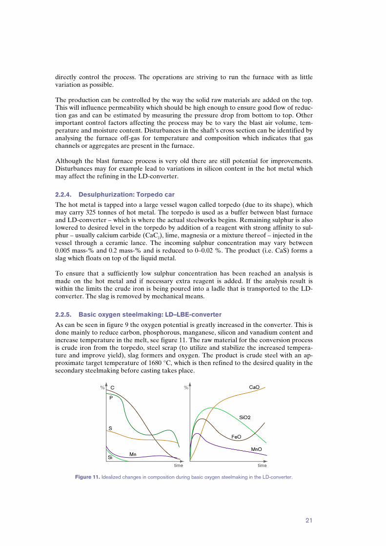
As can be seen in figure 9 the oxygen potential is greatly increased in the converter. This is done mainly to reduce carbon, phosphorous, manganese, silicon and vanadium content and increase temperature in the melt, see figure 11. The raw material for the conversion process is crude iron from the torpedo, steel scrap (to utilize and stabilize the increased tempera-ture and improve yield), slag formers and oxygen. The product is crude steel with an ap-proximate target temperature of 1680 °C, which is then refined to the desired quality in the secondary steelmaking before casting takes place.

Figure 11. Idealized changes in composition during basic oxygen steelmaking in the LD-converter.

22

The furnace is called LD–LBE-converter, where LD is short for Linz and Durrer, the for-mer being the city where the reaction vessel was first installed and the latter the surname of its Swiss inventor3. LBE is short for lance–bubbling equilibrium and refers to the possibility of bubbling inert gas (argon or nitrogen) through the bottom of the vessel, improving the agitation. Through the lance, pure oxygen is blown into the vessel, creating a highly oxidiz-ing potential. Based on an analysis of the liquid crude iron in the incoming ladle, an optimal program for the conversion process is calculated by a heat model which also suggests amounts of scrap, slag formers and oxygen to add. The scrap is added first and then the hot metal, thereafter the lance is lowered and starts to blow 99.5 % pure oxygen into the vessel. This causes sev-eral of the compounds to oxidize, where silicon and manganese are the first ones (not to mention iron, which makes up 94 mass-% of the hot metal). The SiO2-formation is highly exothermic and contributes a lot to the increase in temperature, allowing the scrap to melt. Carbon and phosphorous oxidation also give large contributions to temperature increase. The silica forms the first slag together with MnO and FeO and lowers the melting point for the added slag former CaO. In figure 11 it can be seen that manganese concentration in-creases when the silicon oxidation is complete. The high temperature reduces MnO in the slag by carbon, but during the end of the blow the Mn-concentration decreases again due to a reaction with ferrous oxide:

FeO(slag) + Mn(melt) = MnO(melt) + Fe(l)FeO(slag) + Mn(melt) = MnO(melt) + Fe(l) Phosphorous oxidation is affected negatively by increased temperature which explains why phosphorous content increases at the middle period of blowing. The concentration of FeO in slag increases greatly at the end of the blowing when most of the Si, Mn, C and P have been oxidized. When blowing is over (about 25 minutes) a sample is taken from both the metal and slag. If the concentrations and temperature are acceptable the steel is tapped into a ladle. Care must be taken not to carry over slag from the converter to the ladle, which otherwise would bring impurities to the steel that are very hard to remove (especially re-reduction of phos-phorous and vanadium). Also, deoxidation agents such as ferrosilicon (containing iron sili-cide, FeSi) and aluminium are added to lower the oxygen level.

Important parameters The converter is mainly controlled by changing lance height, oxygen blowing and bottom bubbling with argon and/or nitrogen. The process program chosen is dependant on start and target values for metal composition and temperature. Most crucial during operation is to avoid that the ferrous oxide rich slag – which is very foamy – builds up to high and leaves the vessel. Such an occurrence is called slopping and causes loss of raw material and haz-ardous gas discharge. Several attempts to predict and control slopping have been made with varying levels of success.

2.2.6. Secondary steelmaking: TN-station and ladle furnace

The converted steel is relatively rich in dissolved oxygen and other gases such as nitrogen and hydrogen which must be removed. It will also need adjustments in alloy concentrations which can be done in a variety of equipments and by a range of additions to reach the tar-get analysis for the steel. Gas bubbles or slag inclusions decrease the strength and tough-ness of the finished steel which is detrimental for quality aspects. Gas removal may be done by agitation and vacuum treatment, although oxygen is often precipitated by a reagent ad- 3 According to Sethur (1960), D in LD may also stand for Düsen, which is Voest’s patented jet for oxygen blowing, or Donawitz, which installed the LD-converter shortly after Linz.

23

dition such as FeSi or Al as is done when the LD-converter is emptied. Slag inclusions con-sist of oxides or sulfides originating from the slag, refractory lining or precipitation reac-tions. At SSAB Oxelösund there are two stations used for these types of treatment: TN-station (Thyssen Niederrein or trimningsstation) and the ladle furnace (SU, skänkugn). The TN-station is a rather simple step and gives the opportunity for the following refining steps:

� Desulphurization. � Homogenisation by argon flushing through a ceramic lance or porous plugs in the

bottom. � Alloy addition to meet the demanded analysis and scrap addition to decrease tem-

perature. � Addition of CaSi-wire combined with argon flushing to reduce inclusions. Silicon

binds strongly to oxygen and calcium may react with either oxygen, sulphur or alu-mina inclusions: - Ca(steel) + O(steel) = CaO(slag)Ca(steel) + O(steel) = CaO(slag) - Ca(steel) + S(steel) = CaS(slag)Ca(steel) + S(steel) = CaS(slag) - Ca(steel) + (n + 1=3)Al2O3 = CaO ¢ nAl2O3 + 2=3Al(steel)Ca(steel) + (n + 1=3)Al2O3 = CaO ¢ nAl2O3 + 2=3Al(steel) - CaO(incl:) + 2=3Al(steel) + S(steel) = CaS(incl:) + 1=3Al2O3(incl:)CaO(incl:) + 2=3Al(steel) + S(steel) = CaS(incl:) + 1=3Al2O3(incl:)

The ladle furnace is a comprehensive piece of equipment. In ad-dition to the tools available at TN there are several alternatives for refining:

� Efficient degassing can be achieved by vacuum treat-ment while flushing argon into the liquid steel from the bottom of the vessel.

� Heating possibilities by a set of electrodes creating elec-tric arcs.

� Stirring possibilities by electromagnetic induction for homogenization and slag inclusion modification pur-poses. Stirring is also important for degassing since the ferrostatic pressure is about two atmospheres at the bot-tom of the ladle and would cause too large portions of gas to remain in the liquid steel if there were no circula-tion in the ladle.

Once the analysis shows that the steel meets ordered quality the ladle is transported to the casting machine.

2.2.7. Continuous casting

Good control of the casting procedure is vital for final product quality, i.e. nice surface properties, absence of cracks and pores and a homogenous analysis throughout the finished slab. Correct temperature and absence of air while tapping the steel into the casting equip-ment are important factors. The presence of alloys in the steel affects the solidifying tem-perature in such a way that there exists a solidifying temperature range rather than a fixed temperature. The temperature where the steel begins to solidify is called the liquidus and the temperature when it is a stable solid is denoted solidus. This leads to a phenomenon called segregation where the recently solidified steel does not have the same analysis as the molten steel next to it due to decreased solubility in the solid state for some elements. The segregated elements become enriched in the interior.

Figure 12. Ladle furnace. (Ullmans 2007)

24

The ladle received from secondary steelmaking is placed above a container called tundish which serves as a steel buffer between the ladle and the mould, ensuring a controlled flow and the ability to change ladle while casting. The mould is placed underneath the tundish, see figure 13. The whole process also involves a manoeuvre where the vertically orientated solidifying steel strand is transferred to a horizontal positioning before cutting occurs. The liquid steel flows through a refractory pipe in the bottom of the ladle into the tundish. The top surface of the tundish is covered to protect from air and there may also be internal walls present in the tundish. Their purpose is to reduce the length any remaining inclusion must travel to be captured in the casting powder holding the slag phase – thus more inclusions will be removed and steel quality improved. However, such an arrangement is not present at SSAB Oxelösund. When the tundish is full the steel starts to pour down into the mould through another pipe. The mould is water cooled to promote solidification and the casting powder added to the top of the mould surface keeps the surrounding air away. The outer part of the steel begins to solidify as the temperature decreases. An oscillation movement of the mould promotes im-proved surface properties and prevents the strand to stick at the mould wall. The process parameters are controlled in such a way that the solid shell is thick enough to withstand the ferrostatic pressure (the weight of the liquid steel inside the strand) when the strand leaves the mould and enters the secondary cooling zone where wa-ter jet nozzles produce a water mist that cools the strand. Samples are taken from casting sequences representing T-sorts known as difficult to meet desired quality, and analyzed with respect to the inner structure and composition. When the strand reaches the end of the casting machine it is eventually cut into desired lengths, called slabs. Some slabs are visually inspected for surface cracks. After-treatment depends on the customer’s demands but may imply grinding or storage in a diffusion furnace before they are taken to the rolling mill. However, many slabs may be directly delivered to customer.

Important parameters It is especially the temperature that is important during the casting process. The tempera-ture in the mould should be about 20–25 °C above the liquidus temperature to cover for heat losses, but the most important aspect is to minimize variations. Frequency and ampli-tude of the mould oscillations, cooling water flow, casting speed and steel levels in tundish and mould are other important control factors. A technique called soft reduction is used to minimize the appearance of segregations in the slab centre. The rolls at the end of the cast-ing machine, placed just before the strand’s inner melt solidifies, exert a pressure on the strand which homogenizes the metal composition.

2.2.8. Challenges in the production line

Several of the process steps may be denoted as crucial to reach the desired quality of the steel slabs. The blast furnace needs to deliver crude iron at a reasonably similar composi-tion all the time. High levels of liquid iron inside the shaft will push up the hot blast race-way, causing excessive heating which may burn too much coke and increase refractory lin-

Figure 13. Illustration of tundish and oscillatiing mould. (Ullmans 2007)

25

ing wear. Operational variations may cause extra amounts of desulphurization reagent to be used in the torpedo cars and also extra alloying in the steel plant, which is an economical drawback. The large volume of material passing the blast furnace and the long residence time makes every reduction in raw material use valuable both economically and environ-mentally. In the steelworks, the process in the LD–LBE-converter is of high importance. Decreasing time from tap to tap, avoid slopping, reach the analyze targets and avoid slag carryover during tapping are things that the operation personnel must consider. Careful alloying of the crude steel at tapping from the LD-converter is necessary not to reach compositions higher than tolerated in the T-sort to be produced. The secondary steelmaking will fine-tune the composition, but the closer to final analysis the steel is already after tapping from the LD-converter, the smoother the process will continue. Deoxidation, degassing and ho-mogenisation are also important steps for most T-sorts. An incomplete homogenisation due to insufficient gas bubbling may cause deoxidation agent and inclusions to remain in the steel. In addition to analysis, the crude steel temperature also needs to be accurate enough when the ladle is sent to casting. During casting the temperature in the tundish is of great importance to avoid segregation and achieve good surface quality. If the soft reduction is to work properly there is a need to know where in the strand direction the last molten iron solidifies.

2.3. Previous studies of steelworks using multivariate methods Multivariate methods have been used successfully in a wide variety of applications in the process industry for at least 20 years. Not least have several projects aiming for develop-ment of statistical process control been carried out (e.g. Nomikos & MacGregor 1995). The steel industry has also investigated some process parts with multivariate methods, but it may not always be publicly available. Prediction of slips in the blast furnace has been attempted by Gamero et al (2006) and the development of an expert system for operating the blast furnaces at Corus’ sites in the UK is described by Warren & Harvey 2001. In a study by Bhattacharya (2005) the silicon con-tent in the hot metal produced in the blast furnace was predicted by a PLS model, however with great uncertainty in the predications. A comprehensive study on process control has been carried out with SSAB Oxelösund as one of the primary research objects. The project was called HIPCON, Holistic integrated process control, and was supervised by IVL Swedish Environmental Research Institute4. One application developed within HIPCON is a desulphurization reagent dosage model where the desulphurization step in the torpedo cars was studied with multivariate methods. A model for reagent dosage calculation based on PLS was developed in 2004. A somewhat similar study has been done at Dofasco’s steelwork in Canada, described by Dudzic & Quinn (2002). Another objective for the HIPCON project was to classify LD-converter heats with respect to slopping occurring or not. The results were though not clear enough for certain predic-tions, but valuable information about factors affecting slopping behaviour was achieved. The work was presented in 2005. In a diploma thesis from 1996, Kappel investigates impor-tant factors for temperature decrease after blowing in the LD-converter with PCA and PLS models but bad quality of data deteriorates the result.

4 The HIPCON project was performed within the European Union’s sixth framework programme for research and technological development 2004 – 2006.

26

Secondary steelmaking has not been investigated with PCA or PLS in particular, but a work done by Fernandez et al used Self-organizing maps (SOM) to predict steel quality after ladle treatment. A comprehensive project developing an online monitoring system for the continuous cast-ing stage has been developed at Dofasco’s facilities in Canada (Zhang & Dudzic 2006). The system is able to monitor the whole batch duration; start-up, normal operation and transi-tion phases such as spare part changes. To correct for the different numbers of observations between the occasions studied an indicator variable is used.

27

3. Data treatment and modelling

3.1. Data pretreatment

3.1.1. Data extraction and structure

Historical process data where extracted from databases at SSAB Oxelösund and supplied as Excel files which then were treated further with Microsoft Excel 2003. Availability of blast furnace historical data limited the time period to about six months, from mid August 2007 to mid February 2007, except for crude iron analysis data which were available from January 2006. Data extraction for all steps except the blast furnace was quick and data treatment and modelling first performed for these processes. Blast furnace data where ex-tracted in steps, with the complete set available in April 2007. Each of the Excel files contained data representing only a part of the actual block, such as desulphurization, crude steel analysis after LD-treatment, ladle furnace treatment, casting machine properties and remarks on the slab inner quality. Each of the tables contained one or more key variables useful to match the observations. The heat number in the LD-converter (named LSNR) was chosen as observation id, and the relevant heats for the three T-sorts chosen (T1, T2, T3) were selected within the specific period of time. Figure 14 de-scribes the relationships between the different keys used to match data. It should be noted that the most challenging part is the fact that the crude iron used for a heat in the LD-converter may originate from both blast furnaces and several torpedos.

Figure 14. Schematic drawing of treatment pathways and key variables for each step. Common variable types are analyses for metal and slag, amount of raw material added and operational parameters such as temperatures, gas flows and more. Several different resolu-tions are available:

� Time-based - Raw material additions from end of November were available on an hourly ba-

sis. They were matched with discharge data based on a blast furnace residence time of 7–8 hours: 0.04 x 6 h ago + 0.46 x 7 h ago + 0.46 x 8 h ago + 0.04 x 9 h

ago.

Blast furnace One tapping goes to several torpedos Key: UTNR

Torpedos One torpedo may contains several tappings Keys: TPNR, TPKPJ TPRESA

LD-converter One charge contains of crude iron from sevreral torpedos Key: LSNR

Secondary steelmaking, TN and SU station All charges go to TN but not all goes through SU. A charge may be returned e.g. from SU to TN or LD. Keys: LSNR, SSNR

Continuous casting A casting sequence may consist of several charges. Several slabs are cut from each charge. Keys: LSNR, SSNR, AENR

28

- Operational parameter data for the blast furnace were available as a 24 hour average which was matched to its corresponding discharge.

� Working shift-based

- Raw material additions from end of August were available per working shift. Several discharges are made per working shift and data was matched by letting the first tapping for the shift have material data from previous shift, the second tapping took material data as half of the previous shifts additions plus half of the current shift. A third tapping took all its material additions data from the current shift.

� Heat-based

- All data from LD-treatment and secondary steelmaking and casting data ex-cept slab analysis.

� Slab-based

- Analysis of composition and quality for the slabs casted from a specific heat and sequence. For quality remarks the fraction of faulty slabs was calculated and used when weighting the data to represent LD-heat. For composition analysis the maximum and minimum values and standard deviation within each heat were used as variables.

In order to match data for torpedos with data for LD-treatment a coupling table was con-structed and supplied by SSAB Oxelösund. It consisted of actual mass of the crude iron taken from a specific torpedo and used for a LD-heat and together with the total weight loaded the fraction from each torpedo could be calculated. For blast furnace modelling, datasets using discharge number as observation id (rather than heat number) were used in addition to the ordinary LSNR-weighted data set. That made it possible to study the behavior of the actual process without losing important information. Some graphs visualizing analysis deviations were created using Microsoft Excel.

3.1.2. Variable selection

Some of the variables available were not useful for modelling in their original state, and therefore different approaches were used in order to create useful information from them. Examples of data treatment:

� Filtering data to get only observations corresponding to the time period and T-sorts chosen.

� Deleting unnecessary variables. � Determining whether to use a parameter as variable and/or label. � Creating a new variable from one or more existing ones, for example:

- Treatment time calculated from stop and start timestamp. - Total amount alloy added calculated from alloy number in nth addition and

weight added in nth addition. - Amount of gas added calculated from gas flow and time. - Lance height after nn% of the treatment calculated from lance position before

change related to fraction of treatment time when change occurred. - Deviation from target created from measured value and aim/max/min value. - Relative variables, e.g. amount of reagent per amount of sulphur.

For some of the data processing tasks Excel macros were created using Microsoft Visual Basic. The accuracy of the data tables created by these macros was verified by random sample comparison with original data.

29

3.1.3. Block construction

The process naturally decomposes into five blocks as described in section 2.2.1. Data tables for each block where merged using Microsoft Access 2003 and typical variables can be seen in figure 15. The two letter abbreviations will be used when referring to the different blocks later on.

Figure 15. Illustration of the multiblock model with the different variable types noted. Each data block contained the same observations; for the last four blocks there were 477 observations (Ntot = 477) and for the BF block NBF = 386, due to missing data, especially for August. The Excel files for each block were imported one by one into the modelling software. The number of variables in each block, K , were 58 for BF, 37 for TP, 105 for LD, 153 for SS and 148 for CC, i.e. Ktot = 501. The three T-sorts used in the study constitute subsets of observations as follows: N534 = 181; N723 = 96; N763 = 200. A complete list of variables used, together with a short description, is found in Appendix B: Variable list.

3.2. Modelling Modelling has been carried out using the software Simca-P+ 11.5 from Umetrics AB, Umeå, Sweden. At first, the individual blocks where modelled separately with PCA to identify patterns and variables influencing the quality targets within the particular step. Another important task is to investigate which phenomena that are captured in the princi-pal components in order to interpret the models and especially understand contributions to the hierarchical model. In addition, for some blocks PLS models were created to study par-ticular relationships. Below methods and arguments are presented quite general, only men-tioning details to a small extent. All modelling have been documented separately in Simca-P+ project files and spreadsheet documents.

3.2.1. Block modelling

After importing the whole data table to Simca-P+, a workset is created before a model is fit. When analysing and improving the model it is then possible to create new worksets

BF, blast furnace

TP, torpedo cars

LD, LD-converter

SS, secondary steelmaking

CC, continuous casting

Parameters - oscillations - temperatures - H-diffusion Slab analyses - inner quality - surface qual. - composition

Both TN and SU Additions - alloys - deO agent Parameters - gas bubbling - stirring - heating - vacuum Analyses - steel - tundish

Analyses - crude iron - after conv. Additions - slag formers - alloys - scrap Parameters - lance pos. - oxygen flow - gas bubbling - conv. time

Analyses - before deS - after deS - deviation Additions - CaC2

Parameters - reagent flow - metal weight - temperature

Material data - ore pellets - coke - briquettes - inject-coal - limestone Analyses - crude iron - slag Parameters - air blast - temperature - pressure

SUPER LEVEL MODEL

Slab quality Analysis and temp misses

Slopping Analysis misses

Desulphurisation Crude iron variations

30

based on the original data or an existing model. By default a variable or observation with more than 50% missing values will be excluded from the workset, but for some models the limit was set even higher in order to model information that were seldom registered, e.g. slag analysis after LD-treatment. When fitting the model, Simca-P+’s autofit-function has been used most of the times. It calculates the number of components that are cross-validated according to a set of rules (Umetrics 2002):

1. Component significant if Q2 > b where b is 0 for PLS, whereas in PCA it increases with the number of components calculated, to account for loss in degrees of free-dom.

2. Component significant if Q2var > b for at least

pK variables (or at least one vari-

able for PLS). Q2var is the explained variance for a variable.

3. Only applicable to PCA. A non-significant component according to (1) and (2) may be denoted significant if the next component is significant and they have simi-lar eigenvalues (max 5% difference).

By looking at the R2 and Q2 values for the model and the contributing variables, a brief understanding of the data’s capability of describing the process is achieved. For real proc-esses the level of explained variance is normally rather not very high, especially if the data resolution is low and the process is complex. Sometimes data quality may be a reason to bad statistical properties. In most cases, the workset has been carefully examined for out-liers, e.g. obviously false analysis values, by variable trimming where values below or above a certain limit are excluded. This method should however be used with care, not to remove useful information. Two-dimensional plots of the first two score and loading vectors respectively have been used to reveal the most dominant factors in the data set. This is not always the phenomena of interest, which may be captured in later components as well. For the steelworks blocks, when all T-sorts are included in the model the first score-plot typically shows the T-sort grouping due to differences in treatment and analysis. Therefore models have been made both for the whole set of observations but also for each subset of T-sort specific observa-tions. When considering a components importance it’s fraction of explained variance have been considered. Simca-P+ automatically calculates and shows the Hotellings T 2 ellipsoid which simplifies outlier detection. It is however important to investigate the reason for an obser-vation being located outside the T 2-range. For example, when modelling data from secon-dary steelmaking, observations may not always have the same treatment path, though be-longing to the same T-sort. This will show up in the score plot, sometimes creating outliers. In these cases, the observations have been kept in the workset. Other more obvious outliers have been removed, e.g. lance height registered as zero. The DModX-plot have been used in a similar way as the score-plot. It is possible to find other types of outliers that are not outside the T 2-plot but still deviate from the model. However, it is still important to check the cause for the observations high DModX-value. Relationships between variables have been studied using the loadings where correlations can be detected. Both two-dimensional scatter plots and column plots have been used. To see what factors that influence a specific phenomenon, such as insufficient sulphur removal, the contribution plot is a useful tool. By selecting objects that share the phenomenon of interest in a score-plot of relevant components it is possible to create a column plot of each

31

variables contribution to the selected observations compared to the whole set of observa-tion, where the loadings of respective components are used as weights. Labels and colours that identify patterns and characteristics of the observations have been used as helpful tools in model analysis, as well as object selection to visualize only observa-tions of interest. Table 1 summarizes the most important models created for each block.

Block Model no N K A R2 Q2 Comment

BF BF03.M4 577 56 8 0.73 0.54 PCA, BF2 BF03.M7 371 51 8 0.79 0.58 PCA, BF2, 2007 BF04shift.M11 889 17 (X), 18 (Y) 6 0.83 (X), 0.38 (Y) 0.37 PLS, steel and slag as Y BF04shift.M14 989 55 (X), 5 (Y) 2 0.45 (X), 0.01 (Y) 0.001 PLS-DA for working shift TP TP02.M4 458 31 6 0.71 0.38 PCA TP03.M11 279 21 (X), 3 (Y) 4 0.52 (X), 0.40 (Y) 0.26 PLS, S as Y LD LD05.M7 477 74 7 0.68 0.50 PCA, incl. aim values LD05.M8 477 53 9 0.66 0.29 PCA LDSSCC.M7 477 102 8 0.43 0.21 Analysis outliers removed LDslp.M1 439 74 (X), 1 (Y) 2 0.32 (X), 0.11 (Y) 0.13 PLS, slopping as Y SS SS01.M1 477 192 3 0.38 0.34 PCA LDSSCC.M16 477 124 4 0.53 0.50 PCA TPLDSSCC.M21 477 115 5 0.61 0.55 PCA TPLDSSCC.M22 211 115 4 0.55 0.47 PCA, only SU-heats TPLDSSCC.M24 452 35 (X), 1 (Y) 2 0.34 (X), 0.52 (Y) 0.47 PLS, TN temp. diff. as Y CC CC03.M7 472 205 6 0.48 0.38 PCA LDSSCC.M18 475 134 5 0.54 0.47 PCA LDSSCC.M30 469 126 (X), 5 (Y) 3 0.50 (X), 0.16 (Y) 0.12 PLS, slab quality as Y

Table 1. Summary of properties for the most important block models created. Model names refer to the project files. The blast furnace models have discharge number as observation id while the other blocks use LD-heat number as unique identification.

3.2.2. Hierarchical modelling

When preparing to build a hierarchical model for the whole process the block models were chosen as base models in Simca-P+. This enabled the score vectors of each model to be se-lected as variables when creating the workset for a new model. The fraction of explained variance for a specific component has been an important factor when selecting components to include in the model. Several combinations were tried out but it is normally the first few score vectors in a model that reveals the important information which is possible to use in a super-level model. Four models were made, one containing all three T-sorts and then one for each T-sort. Table 2 summarizes the hierarchical models.

T-sort N K A R2 Q2 Comment

All 477 15 2 0.37 0.07 First component insignificant T1 181 10 2 0.36 – 0.06 First component insignificant T2 93 10 2 0.50 0.12 Two significant components T3 200 13 2 0.34 – 0.07 No significant components

Table 2. Summary of properties for the hierarchical models created.

32

4. Results

4.1. Block modelling

4.1.1. Blast furnace (BF)

Graphs created to visualize production variations in crude iron composition for important elements show that silicon and sulphur deviations from aim values are frequent – every third discharge contains to high silicon and/or sulphur concentration. Too low manganese content is also common while vanadium, chromium and phosphorous exceeding are below five percent of the taps. In total, 56% of the crude iron discharges do deviate from the analysis target interval for one or more elements.

Blast furnace tappings: deviations from target analysis in crude ironJanuary 2006 – February 2007

0%

5%

10%

15%

20%

25%

30%

35%

Si Mn P S Cr Cu Ni V

Element

Percent

BF2 above max BF4 above max BF2 below min BF4 below min Deviations from analysis target, blast furnace 2

(above max/below min)

-0.2

-0.1

0

0.1

0.2

2006-01-01

2006-02-01

2006-03-01

2006-04-01

2006-05-01

2006-06-01

2006-07-01

2006-08-01

2006-09-01

2006-10-01

2006-11-01

2006-12-01

2007-01-01

2007-02-01

Date

Deviation in m

ass percent

DiffSi DiffMn DiffS

Deviations from analysis target, blast furnace 4(above max/below min)

-0.1

0

0.1

2006-01-01

2006-02-01

2006-03-01

2006-04-01

2006-05-01

2006-06-01

2006-07-01

2006-08-01

2006-09-01

2006-10-01

2006-11-01

2006-12-01

2007-01-01

2007-02-01

Date

Mass percent

DiffSi DiffMn DiffS

Figure 16. Blast furnace crude iron composition target deviations (above max/below min). Above: Accumulated, below left: time-resolved for BF2, below right: time-resolved for BF4.

Positive value axes are cropped for the two lower graphs. These deviations are more frequent under certain times of operation. When examining model BF03.M4 it is shown that periods of unstable operation in blast furnace 2 are mani-fested as outliers both in the score and distance-to-model plots. When comparing the ob-servations from one such period (in November–December) with the average the main con-tributors are high silicon content, low manganese oxide content and low top gas flow. A similar analysis for blast furnace 4 shows fewer and shorter periods of unstable operation, and the contributors are higher silicon and titanium content in crude iron and higher sul-

33

phur content in slag. The time periods can be seen in the distance-to-model plot in figure 17.

-14

-12

-10

-8

-6

-4

-2

0

2

4

6

8

10

12

-10 0 10 20

t[2]

t[1]

BF04shift.M4 (PCA-X), BF2, improvedt[Comp. 1]/t[Comp. 2]


SIMCA-P+ 11.5 - 2007-05-23 13:35:08

0

1

2

3

20

06

-08

-31

20

06

-09

-05

20

06

-09

-10

20

06

-09

-15

20

06

-09

-20

20

06

-09

-24

20

06

-09

-28

20

06

-10

-02

20

06

-10

-05

20

06

-10

-09

20

06

-10

-13

20

06

-10

-16

20

06

-10

-28

20

06

-10

-31

20

06

-11

-03

20

06

-11

-06

20

06

-11

-10

20

06

-11

-13

20

06

-11

-17

20

06

-12

-01

20

06

-12

-04

20

06

-12

-14

20

06

-12

-17

20

06

-12

-21

20

06

-12

-24

20

06

-12

-27

20

07

-01

-00

20

07

-01

-03

20

07

-01

-07

20

07

-01

-10

20

07

-01

-13

20

07

-01

-17

20

07

-01

-20

20

07

-01

-24

20

07

-01

-28

20

07

-02

-01

20

07

-02

-04

20

07

-02

-09

20

07

-02

-13

20

07

-02

-16

DM

od

X[8

](N

orm

)

Obs ID (Datum)

BF04shift.M4 (PCA-X), BF2, improvedDModX[Last comp.](Normalized)

M4-D-Crit[8] = 1.203 1 - R2X(cum)[8] = 0.2253

D-Crit(0.05)

SIMCA-P+ 11.5 - 2007-05-23 13:34:44

Figure 17. Unstable operation in blast furnace 2. The red squares represent the same observations in both plots. In the distance-to-model plot (to the right) the time periods can be seen: (a) during start-up in August 2006, (b) after

shut-down in October, (c) unstable operation in November – December. The models built in project BF03 also showed other results regarding factors influencing crude iron composition:

� By looking at the loadings for M7 it was seen that phosphorous is negatively corre-lated to sulphur content in crude iron.

� Sulphur content in the slag is positively connected to basicity and negatively to temperature in shaft and air blast flow, temperature, oxygen content and also top gas flow.

The PLS models in project BF04shift were used to predict metal and slag analyses based on material additions per working shift and operational parameters per day average which should be considered as poor data resolution. The model residuals are therefore very large for many response variables, but measures such as lime, dolomite and silicon oxide content in slag and phosphorous and chromium content in the metal have reasonably good predic-tion properties. Explained variance for the prediction sets are given for both furnaces in figure 18.

Q2 for Y-variables, observations from predictionset

-0.4

-0.2

0

0.2

0.4

0.6

0.8

C Si Mn P S_iron Cr Cu Ni Ti V CaO SiO2 MgO FeO MnO S_slag B2 B3

BF2 BF4

Figure 18. Explained variance for response variables (Q2varQ2var) – observations from prediction set.

34

Performing discriminant analysis on material data based on working shift does not imply that any differences exist between the working shifts. This is illustrated in figure 19.

-6

-4

-2

0

2

4

6

8

10

12

14

16

-10 0 10 20

t[2

]

t[1]

BF04shift.M14 (PLS-DA)t[Comp. 1]/t[Comp. 2]Colored according to classes in M14


Class 1Class 2Class 3Class 4Class 5

SIMCA-P+ 11.5 - 2007-05-23 14:20:46

Figure 19. Score plot showing the discriminant analysis made for working shifts in the blast furnace. No regular pattern could be found.

4.1.2. Desulphurization (TP)

A score plot of the first two components in model TP02.M4 shows a clear time drift for the heat weighted observations. This is due to compositional variations in the crude iron re-ceived from the blast furnace – observations from August and September have higher phosphorous and lower manganese and chromium content than the average observation. The opposite is true for observations from January and February compared to average. Plotting the incoming compositions for P, Mn and Cr shows an overall increasing time-trend for Mn and Cr and a decreasing time-trend for P. Plotting contributions to scores for observations with high residual sulphur content (re-maining sulphur after main injection of calcium carbide – ordered content > 0) does not give any easily interpretable results. Notable is that the incoming sulphur content does not affect the ability to reach target concentration. The explained variance for sulphur content (TAS2) has been low in the PCA models created. For TP02.M4 R2

TAS2 = 0:71 and Q2

TAS2 = ¡0:14. However, introduction of a variable for the absolute sulphur amount (SABS_E) improves the model and Q2

TAS2 is then calculated to 0.33 (TP03.M2). A PLS model was fitted in order to reveal important factors for desulphurization (TP03.M11). The response variables were sulphur concentration after treatment, absolute

amount after treatment and deviation from ordered sulphur content. Looking at the coeffi-cient plot shows that most variables are not significant. The contributions (significant vari-ables only) are as follows (‘+’ indicates positive correlation; ‘–’ indicates negative correla-tion).

� Sulphur concentration and absolute S amount after treatment - ordered sulphur content - hot metal weight

� Deviation from ordered sulphur content - chromium content - carbon content - ordered sulphur content

35

This PLS model had much better statistical properties for TAS2 than the PCA models de-veloped. R2

TAS2 = 0:54 and Q2TAS2 = 0:40.

4.1.3. LD–LBE converter (LD)

Studying model LD05.M1 shows that the variables describing scrap additions does not con-tribute much to the model. This may be caused by the many different scrap numbers used in the dataset, i.e. each number is not used enough times to bring meaningful information into the model. When trying to find reasons for missed analysis after LD-treatment, it can first be estab-lished that the incoming crude iron composition may contribute. In the left part of figure 20 the loadings p3p3 and p4p4 for LD05.M7 can be seen. Variables for incoming crude iron analysis are represented by black dots and it can be seen that they are affecting both t3t3 and t4t4. The score plot to the right implies that the reason for the heat in the upper left corner being an analysis miss may be due to high levels of molybdenum, chromium, manganese or nickel (or low levels of variables in the opposite direction). In this case, the steel analysis after LD-treatment showed high nickel level.

-0.2

-0.1

-0.0

0.1

0.2

0.3

-0.3 -0.2 -0.1 -0.0 0.1 0.2 0.3

p[4

]

p [3]

LD05.M7 (PCA-X), Removed vars with neg Q2p[Comp. 3]/p[Comp. 4]Colored according to Var ID (Primary)

R2X[3] = 0.0698088 R2X[4] = 0.0604882

OSANC

OSANSi

OSANMn

OSANP

OSANCr

OSANNi

OSANMo

OSANV

LAANC230

LAANSi230

LA ANMn230

LA ANP230

LA ANS230LAA NCr230

LA ANMo230LAANV 230

LD3N2TO

LD3A RTO

LD6DOTO

LD6FUTO

LD6KATO

LD6MATO

LD6O2TO

LD7FPTP1

LSINSVKTLSVEV IKT

LAH35

LAH50

LA H60LAH80

BEHTIDTOT

OSA NTi

BLANT

FUANT

MAA NT

LD7FPTP2LD7O2FH1

LD7O2FH4

LD2FPTP1

LD2RATP

LD8A LBE

LDLGE5018

LDLGE5017

LDLGE5061

LDLGE5045

LDLGN5307

LDLGN5308

LDLGN5008

LDLGN5218

LD7SONT

LD9SLE

LD2TPTB

LD1CH001LD1CH002

LD1CH003

LD1CH006

LD1CH008LD1CH026LD1CH027

LD1CH028

LD1CH031

LD1CH033LD1CH051LD1CH052

LD1CH053

LD1CH054

LD1CH055

LD1CH056

LD1CH057

LD1CH058

LD1CH059

LD1CH061

LD1CH067

BLTITOT

SIMCA-P+ 11.5 - 2007-05-23 14:30:40

-6

-4

-2

0

2

4

6

8

10

-20 -10 0 10

t[4

]

t[3]

LD05.M7 (PCA-X), Removed vars with neg Q2t[Comp. 3]/t[Comp. 4]Colored according to Obs ID (ANABOM230)


Default

1*

SIMCA-P+ 11.5 - 2007-05-23 14:33:09

Figure 20. Loadings and scores for LD05.M7. Crude iron composition variables are seen as black dots and labels in the left plot. Observation deviations from target analysis are shown in green in the right plot.

There are also six other analysis misses; one heat is too high in carbon, nitrogen and sul-phur and another too high in manganese and too low in nitrogen. Four heats are too high in phosphorous. These observations are found in the middle of the score plot, with only small dependencies on incoming crude iron composition. A plot for the four high P heats shows the following contributions:

� High incoming phosphorous content, low silicon and titanium. � Low amount of lime and oxygen added, very low estimated slag amount. � Short blowing time.

The result confirms that low silicon content only allows a small amount of slag formers to be added since the desired basicity otherwise would be exceeded. As phosphorous cleaning is an important task for the slag, the LD-treatment is not able to meet desired P level. Analysing model LDSSCC.M7 and plotting the score’s t2t2 and t3t3 for only the observations where severe slopping has been registered, a slightly skew representation toward the lower right corner can be seen (figure 21). When studying the loading plot for the same compo-nents and the contribution plot for the whole group of slopped heats compared to the aver-age, it can be seen that variables describing estimated amount of slag, total treatment time, blowing time, additions of lime, dolomite and oxygen are partly responsible for this skew-

36

ness. A slopped heat will naturally demand longer treatment time since the decarburization rate needs to be decreased to control the process. The slag formers may be due to high sili-con content. Slopping prediction gives a result comparable to the one achieved in the HIP-CON project.

-8

-6

-4

-2

0

2

4

6

-7 -6 -5 -4 -3 -2 -1 0 1 2 3 4 5 6 7 8

t[3

]

t[2]

LDSSCC.M7 (PCA-X), LDt[Comp. 2]/t[Comp. 3]Colored according to Obs ID (LD9KOK)


y=-0.1711*x-1.02

R2=0.04002

SIMCA-P+ 11.5 - 2007-05-23 14:49:01

-2

-1

0

1

2

LS

INS

VK

TL

SV

EV

IKT

OS

AN

CO

SA

NS

iO

SA

NM

nO

SA

NP

OS

AN

SO

SA

NC

rO

SA

NN

iO

SA

NM

oO

SA

NV

OS

AN

Ti

OS

AN

Cu

LD

3N

2T

OL

D3

AR

TO

LD

6D

OT

OL

D6

FU

TO

LD

6K

AT

OL

D6

MA

TO

LD

6O

2T

OL

D7

FP

TP

1L

D7

TP

TP

1L

D1

TN

TE

BL

TIT

OT

BL

AN

TB

EH

TID

TO

TF

UA

NT

KA

AN

TL

AH

00

LA

H3

5L

AH

50

LA

H6

0L

AH

80

MA

AN

TL

D2

RA

TP

LD

8A

LB

EL

DL

GN

50

63

LD

LG

N5

30

7L

DL

GN

53

08

LD

LG

N5

00

8L

DL

GN

52

18

LD

LG

N6

50

1L

D7

SO

NT

LD

7S

ON

OL

D7

SO

NC

LD

DO

LA

NT

LD

9S

LE

GA

Ca

OG

AS

iO2

GA

Al2

O3

GA

Mg

OG

AF

eO

GA

Mn

OG

AP

2O

5G

AS

GA

Cr2

O3

GA

V2

O5

GA

TiO

2G

AB

as

KT

MIS

S2

30

KT

MA

TT

23

0

Sc

ore

Co

ntr

ib(G

rou

p -

Av

era

ge

), W

eig

ht=

p2

p3

Var ID (Primary)

LDSSCC.M7 (PCA-X), LDScore Contrib(Group - Average), Weight=p[2]p[3]

SIMCA-P+ 11.5 - 2007-05-23 14:52:40

Figure 21. Score plot (t2 and t3, left) and contribution plot (right) for heats registered with severe slopping.

4.1.4. Secondary steelmaking (SS)

A quick first model (SS01.M1) shows that the T-sort’s are clearly visible also in the secon-dary steelmaking. This is quite obvious since the quality targets and treatment paths are well established for each T-sort. For example, T-sort T3 and T2 are seldom treated in the ladle furnace while T1 almost always are. That is captured in the first two model compo-nents. Plotting scores t3t3 against t4t4 shows distinct observation groupings – not only caused by T-sorts but also sub-groupings due to alloys added (figure 22).

-8

-6

-4

-2

0

2

4

6

-8 -7 -6 -5 -4 -3 -2 -1 0 1 2 3 4 5 6 7 8 9

t[4

]

t[3]

LDSSCC.M16 (PCA-X), EB: From M2, neg Q2's removed. ** Preferred **t[Comp. 3]/t[Comp. 4]Colored according to value in variable blk_LDEBGJ(EBSULGN5401)


T3 T3

T1T1

T3

T3T3T3

T1T1T1

T1T1T1

T3T3

T3T3T3T3T3T3T3

T1

T3T3

T3T3T3T3

T2

T2T2

T3

T3

T1T1

T1

T3 T3

T1

T1T1 T1T1T1 T1

T3

T1

T3

T1

T1

T2

T2

T2

T3

T3

T3

T3

T1T1

T1

T3

T1T1

T2T2

T2

T3T3

T3

T3

T3T1

T2

T1

T3

T1 T1

T1

T2T2

T2T2

T1T1

T1

T3T3 T3T3

T2

T1 T1

T3

T3

T2T2 T2T2

T1

T1

T2

T3

T3T3

T3T3

T3T3T3 T3

T1

T1

T3 T3

T3

T1 T1T3

T3

T3T3T3T3

T1T1

T3T3

T1

T1T3

T3T3

T2

T2

T2

T3T3

T3T1T1

T2T2

T2T2T2

T1

T1

T1

T1

T2

T2T2T2

T2 T2

T1 T1T1 T1

T1T1

T1T1T1

T2

T1T1T1T1

T1T1

T3

T3T3

T3T3

T3

T3T3T3

T3

T3

T3T3T3

T3

T1T1

T1T1

T2

T2

T1T1

T2

T2

T1

T2T2

T2 T2

T2

T2T2T2 T2

T3

T3T3

T3

T1

T1

T1

T1

T2

T2

T2

T3

T3

T3

T3T3

T3T3

T3

T1

T1

T1T1

T3T3 T3T3

T3

T1

T1 T1

T3 T3T3

T2T2

T3T3

T1T1

T2

T3

T3

T2

T3

T3

T1

T2 T2T2

T3T3

T3

T1

T2

T2T2

T3T3T3

T2

T2

T1

T2T2

T2

T2

T3

T2

T3

T1

T3

T3

T3

T1

T1

T2

T3

T1

T2

T3

T3

T3T3

T1

T2T2 T2

T3

T3

T1T1

T3

T1

T3

T1

T1

T1

T2T2

T3T3

T3

T3T3

T3

T1T1

T1

T1

T3 T3

T1T1

T3T3

T2

T1 T1T1T1

T3T3T3

T1

T1

T3T3T3

T1

T1

T1

T1

T3

T3T3

T2

T1T1

T1

T2

T2

T3T3T3

T3

T3

T1

T1

T2T2

T3

T3

T3

T3

T1T1T1

T1 T1

T1

T1

T3T3

T3

T3T3

T3 T3T3

T2T2T2

T1

T1T1

T1

T1

T1T1T1T1T1

T1 T1T1

T2

T2

T3T3 T3T3

T3

T1

T2

T2

T3

T3T3

T1T1

T3T3

T3T3 T3T3T3

T2 T2

T3

T1T1T1

T1T1

T3T3T3

T1T1

T2T2 T2

T1

T1 T1 T1

T2

T2

T1

T1

T2

T3

T3

T1T1

T3

T3

T3T3

T3T3

T3

T3

T1T1T1

T1 T1 T1

T1 T1

T3T3

T1

T1T1

T1T1

T1

T1

T1T1

T3

T3

T1

T1T1

SIMCA-P+ 11.5 - 2007-05-23 15:04:37

-8

-6

-4

-2

0

2

4

6

-8 -7 -6 -5 -4 -3 -2 -1 0 1 2 3 4 5 6 7 8 9

t[4

]

t[3]

LDSSCC.M16 (PCA-X), EB: From M2, neg Q2's removed. ** Preferred **t[Comp. 3]/t[Comp. 4]Colored according to value in variable blk_LDEBGJ(EBTLE5030)


T3 T3

T1T1

T3

T3T3T3

T1T1T1

T1T1T1

T3T3

T3T3T3T3T3T3T3

T1

T1

T3T3

T3T3T3T3

T2

T2T2

T3

T3

T1

T1

T1T1

T2

T1T1

T2

T2

T1

T2T2

T2 T2

T2

T2T2T2 T2

T3

T3T3

T3

T1

T1

T1

T1

T2

T2

T2

T3

T3

T3

T3T3

T3T3

T3

T1

T1

T3 T3T3

T1 T1

T1

T1

T2T2

T2T2

T1T1

T1

T3T3 T3T3

T2

T1 T1

T3

T3

T2T2 T2T2

T1

T1

T2

T3

T3T3

T3T3

T3T3T3 T3

T1

T1

T3 T3

T3

T1 T1T3

T3

T3T3T3T3

T1T1

T3T3

T1

T1

T1T1

T3T3 T3T3

T1

T1 T1

T3 T3T3

T2T2

T3T3

T1T1

T2

T3

T2T2 T2T2

T3T3

T2

T2T2

T3T3T3

T2

T2

T2T2

T2

T2

T3

T2

T3

T1

T3

T3

T3

T1

T1

T2

T3

T2

T3

T3T3

T2T2 T2

T3T3

T1

T3

T3

T3T3

T2

T2

T2

T3T3

T3T1

T2T2

T2T2T2

T1

T1

T1

T1

T2

T2T2T2

T2 T2

T1 T1T1 T1

T1

T1T1

T1

T1T1

T1

T1

T2

T1T1T1T1

T1T1

T1T1

T3T3

T3T3

T3

T3T3T3

T3

T3

T3T3T3

T3

T1T1

T2

T1

T3

T3

T1

T3T3

T1

T1

T2

T2

T2

T3

T3T3

T3 T3

T3

T1T1

T1

T1

T3

T1T1

T2T2

T2

T3

T3

T3

T3

T3

T3T1

T1

T2

T1

T1

T1

T1

T2T2

T3T3

T3

T3T3

T3

T1T1

T1

T1

T3 T3

T1T1

T3T3

T2

T1 T1T1T1

T3T3T3

T1

T1

T3T3T3

T1

T1

T1

T1

T3

T3T3

T2

T1T1

T1

T1

T2

T2

T3T3T3

T3

T3

T1

T1

T2T2

T3

T3

T3

T3

T1T1T1

T1 T1

T1

T1

T3T3

T3

T3T3

T3 T3T3

T2T2T2

T1

T1T1

T1

T1

T1T1T1T1T1

T1 T1T1

T2

T2

T3T3 T3T3

T3

T1T1

T2

T2

T3

T3T3

T1T1

T3

T3T3

T3T3 T3T3T3

T2 T2

T3

T1

T1T1

T1T1T1

T3T3T3

T1T1

T2T2 T2

T1

T1 T1 T1

T2

T2

T1

T1

T2

T3

T3T3

T1T1

T3

T3

T3T3

T3T3

T3

T3

T1T1

T1T1

T1T1 T1 T1

T1 T1

T3T3

T3

T1

T1T1

T1T1

T1

T1

T1T1

T1

T3

T3

T1

T1T1

SIMCA-P+ 11.5 - 2007-05-23 15:05:37

Figure 22. Left: Coloured according to if SU alloy 5401 (CaSi wire) has been added (brown observations). All three T-sorts have observations that used more or less of this alloy. Right: Coloured according to if TN alloy 5030 (FeV)

was added (brown observations). All three T-sorts have groups of observations that used this alloy. Remaining three groups of observations are mainly due to the TN-alloy 5035 which is FeNb. It should be noted that other alloys also contribute to the observation groupings. Examining model LDSSCC.M16 by plotting scores t1t1 and t3t3 and loadings p1 and p3 (figure 23) shows that almost all heats with negative deviations from aim temperature at TN are sent to SU for heating. It is also shown that T-sort T2 and T3 are similar to each other (with respect to Ti, Si, V, C, Mo, Al and P) but dissimilar to T1.

37

-8

-6

-4

-2

0

2

4

6

8

-14 -13 -12 -11 -10 -9 -8 -7 -6 -5 -4 -3 -2 -1 0 1 2 3 4 5 6 7 8 9 10 11 12 13 14

t[3

]

t[1]

LDSSCC.M16 (PCA-X), EB: From M2, neg Q2's removed. ** Preferred **t[Comp. 1]/t[Comp. 3]Colored according to value in variable blk_LDEBGJ(KTMISS234)


Series (Variable KTMISS234)

Missing-74 - -10-10 - 1010 - 132

T1

T2

T1

T1

T3

T3

T2

T3T3

T1

T3

T1

T3

T3

T2

T3

T3 T3

T1

T2

T2

T3

T3

T1T1

T3T3

T1

T1

T1

T2

T3

T1

T1 T1T1

T3

T1

T3

T2

T2

T2T3

T1T1

T1

T1

T2T2 T3

T3

T1

T1

T1

T2

T2

T3T3

T3

T3T3

T1

T1

T3

T1

T3

T1

T1

T1

T1

T3T3T3

T1

T1

T1T1

T1

T3

T3T3T2

T1T1

T1

T1

T2

T2T3T3T3

T3T1

T2

T3 T3

T3

T1T1T1

T1T1

T1

T3T3T3T3

T2

T1

T1

T1

T1T1

T1

T2

T2

T3

T3T3

T1

T1

T2

T2

T1 T1

T3

T3T3T3

T3

T1

T1 T1

T1

T1T1

T3

T3 T3

T1

T2

T2

T1

T1T1

T2T3

T1

T3 T3T3T3

T3T3

T1T1

T1

T1

T1T1

T1

T1

T3T3

T1

T1

T1

T1

T1

T1

T1

T3T3

T1T1 T1

T3T3 T3T3T3

T3

T1T1 T1T1

T3T3T3T3

T3

T3T3T3

T3T3

T1 T1

T3

T1

T1

T2

T1T1

T3 T3

T3

T3

T2

T1T1

T3T3

T2T2

T1

T3T3

T3

T3

T1

T1

T3

T3

T1

T3T3

T1

T3

T3

T2T2

T1T1

T2T2

T2

T2

T1

T1

T1

T1

T1

T1T1

T2

T1 T1

T3T3

T3T3

T1

T1

T2

T2

T1

T2

T2T2T2

T3

T1

T2T2

T2

T3T3

T3

T1

T3

T1

T3T3

T3

T3

T1T1

T2

T2T2

T3

T3

T1

T2

T3

T3

T1

T1

T2

T1

T3

T1T1

T3

T2

T1

T3

T2

T2T2

T2

T2T3

T1

T2T2

T3

T1

T1

T3T3T3

T2T2

T1T1

T1

T1

T1

T1

T2

T3

T3

T3

T3

T3

T3

T3

T3

T1

T2T2

T1

T2

T2

T3

T1

T3

T1

T1

T3

T1

T1T1

T3 T3T3

T1

T3T3

T2T2T2

T1

T3T3

T1

T2

T2

T1

T2 T2T2

T3T3

T3

T3T3T3

T1

T3

T3

T3

T3

T3

T1

T1

T3

T3

T2T2

T3T3

T1

T2 T2

T2

T1

T1

T2T2

T1T1

T1T1T1

T1

T1

T3T3T3T3

T3T3T3 T3T3

T1

T1T1T1

T2

T2

T1

T2

T2T2

T2

T3

T3

T1

T1

T1

T3

T3

T3T3

T1T1

T3

T3

T3

T1T1

T3 T3

T2 T2

T3

T1 T1

T2T2

T3

T3

T3

T3

T3

T3

T2

T1

T3

T2T3

T3 T3T3

T2T3

T3

T3

T3

T1T1

T3T3

T2

T3

T3

T2

T3

T2

T1

T1

T3

T3

SIMCA-P+ 11.5 - 2007-05-23 15:10:49

-0.2

-0.1

-0.0

0.1

0.2

-0.1 0.0 0.1

p[3

]

p [1]

LDSSCC.M16 (PCA-X), EB: From M2, neg Q2's removed. ** Preferred **p[Comp. 1]/p[Comp. 3]Colored according to Var ID (Primary)

R2X[1] = 0.248958 R2X[3] = 0.0903976

Defaultebs*ebt*anan*ebv*

EBCHNST

KTMA TT234 KTMISS234

KTMATT236

KTMATT321

KTMA TT341_

KTMISS341_

EBSXNTSEBSULGN500

EBSULGN501

EBSULGN502

EBSULGN503

EBSULGN503

EBSULGN504

EBTBGASA NT

EBTBLTITOTEBTGA SMGDEBTTLTR2EBTVSUM

EBTLE5007

EBTLE5018

A NANC1

A NANSi1

ANA NMn1

A NANP1

ANANS1

A NANCr1

ANANMo1

EBSULGN506EBSULGN512

EBSULGN521

EBSULGN523

EBSULGN523

EBSULGN530

EBSULGN540

EBSULGN660EBSULGN661 EBSXLTS

EBTLE5021

EBTLE5030

EBTLE5035

EBTLE5045EBTLE5121

EBTLE5230

EBTLE5236

EBTLE5303

EBTLE5401

EBTLE5499

EBTXLTSEBTXTESL

EBTSTTV

ANA NV1

A NANTi1

A NANCu1

A NANA l1

ANANNb1

ANANB1

ANANN1

ANA NZn1

ANA NCa1

A NANCo1

ANANC2

ANA NSi2

ANANMn2

ANANP2

ANANS2

A NANCr2

A NANMo2

ANA NV2

ANANTi2

A NANCu2

ANANAl2

A NANNb2

ANANB2

A NANN2

ANA NZn2

A NANCa2

ANA NCo2ANA NSn2

ANA NH1

A NANH2

EBV HBHTEBVEA NT

EBV ETOTI

EBVHKWT

EBVHKWTOT

EBVGBTOTI

EBV HSB01

EBVHSB02 EBV HSB03

EBV HSB04

EBV FSTOTIEBVACBEHEBV HANG

EBVHSTV

EBV HKRNS

SIMCA-P+ 11.5 - 2007-05-23 15:13:56

Figure 23. Temperature deviations for secondary steelmaking. Left: Score plot coloured according to each observa-tion’s deviation from aim temperature. Blue ones are more than 10ºC below and brown ones more than 10ºC above target. Right: Loading plot coloured according to variable type. Green variables belong to TN station, red variables belong to SU station, blue variables represent steel analysis and black variables represent temperature measures.

Using model TPLDSSCC.M24 to model causes for temperature deviations at TN it can be seen (figure 24) that factors connected to positive deviations are e.g. alloy 5499 (scrap addi-tions for cooling) and heat weight. Additions of alloy 5303 (aluminium wire) and synthetic slag are related to negative deviations from aim temperature.

-0.3

-0.2

-0.1

-0.0

0.1

0.2

0.3

0.4

-0.2 -0.1 -0.0 0.1 0.2 0.3

w*c

[2]

w*c[1]

TPLDSSCC.M24 (PLS), LDAN+TN, PLS for KTMISSw*c[Comp. 1]/w*c[Comp. 2]Colored according to model terms

R2X[1] = 0.271943 R2X[2] = 0.0703439

XY

LAANC230

LAANSi230

LAANMn230

LAANP230

LAANS230

LAANCr230

LAANNi230

LAANMo230

LAANV230

LAANTi230

LAANCu230

LAANAl230

LAANNb230

LAANN230

LAANSn230

EBTBGASANT

EBTBLTITOT

EBTGASMGD

EBTTLTR2

EBTVSUM

EBTLE5007

EBTLE5018

EBTLE5030

EBTLE5035

EBTLE5045

EBTLE5121

EBTLE5230EBTLE5236

EBTLE5303

EBTLE5401

EBTLE5499

EBTXLTS

EBTXTESL

EBTSTTV

KTMISS234

SIMCA-P+ 11.5 - 2007-05-23 15:26:27

Figure 24. Loading weights plot for temperature deviations at TN. In model TPLDSSCC.M22 reasons for temperature deviations at SU or casting were inves-tigated but no obvious reasons could be found.

4.1.5. Continuous casting (CC)

The difference in analysis between the T-sorts is evident in this last process step, as can be seen in figure 25. The score plot for model CC03.M7 shows distinct groupings, mainly due to differences in final tundish analysis but also other factors such as casting settings.

38

-12

-10

-8

-6

-4

-2

0

2

4

6

8

10

12

-10 0 10

t[2

]

t[1]

CC03.M7 (PCA-X), CC, all T-sortst[Comp. 1]/t[Comp. 2]Colored according to Obs ID (LD1TSRT)


SIMCA-P+ 11.5 - 2007-05-25 12:19:28

Figure 25. T-sort groupings in the continuous casting block.

To avoid correlations caused by T-sort differences, one model for each T-sort was created, but the statistical properties became very poor due to the lack of variation in data. There-fore the three T-sorts were modelled together – which is necessary to keep in mind when analyzing the results. Table 3 shows estimated relations between the T-sorts for different properties, based on score contributions between the groups.

Property Less/lower More/higher

Temperature T1 T2 T3

Casting weight T1 T2 T3

Mould oscillations T1 T3 T2

Mould engine current T2 T1 T3

Mould width T1 T3 T2 Mould piston stroke (true value) T2

T1 T3

Slab inner faults T1 T3 (centre quality) T2 (firm side)

T2 (centre quality) T3 (firm side)

Slab visual faults T1 T3 T2

Table 3. Estimated differences between T-sorts at casting. When trying to capture reasons for quality problems loadings for the model LDSSCC.M18 were analyzed. Positive correlation exists between fraction of slabs with visual faults and casting data such as piston stroke, mould oscillations, sculls and number of heats in tundish. Internal quality problems are correlated to tundish temperatures and slab analyses. Further modelling was performed to get more information about causes for quality problems. A PLS-model where slab analysis data were replaced by analysis data from tundish (LDSSCC.M30) was analyzed. Results are presented for visual slab quality and segrega-tions – statistical properties for halfway crack at firm side were to poor for reliable inter-pretation to be done.

� Fraction of slabs with remarks on visual quality (data table AMNVFEL) + Positive correlation: tundish analysis for Si, Ti and N, casting weight, true

mould thickness, oscillations, common length of mixed zone and maximum slab width.

- Negative correlation: tundish analysis for C, Mo, V and Al, mould piston stroke.

39

� Slab centre quality remarks (variable PRCENBET)

+ Positive correlation: tundish analysis for Si, Ti and N, casting weight, true mould thickness, tundish temperatures, oscillations and maximum slab width.

- Negative correlation: tundish analysis for C, Mo, V and Al, mould piston stroke.

� V- segregation width (variable PRBKVSEG)

+ Positive correlation: common length of mixed zone, - Negative correlation: casting weight, total casting time, number of heats in tun-

dish, tundish temperatures. The fact that there are observations belonging to different T-sorts in the model is clearly an aggravation. As can be seen in table 3, many of the factors influencing the quality variables also vary between T-sorts which make interpretation hard. The main conclusion is there-fore that visual quality is connected to casting parameters such as oscillations and inner quality to tundish temperature and steel analysis.

4.2. Hierarchical modelling The hierarchical model containing all observations models the differences between the T-sorts (figure 26), though the statistical properties are poor as stated in table 1 on page 31. The result may be summarized as follows:

� Blast furnace and desulphurization data does not contribute to T-sort differences (i.e. there are no T-sort specifications in these blocks, except for S content).

� LD-treatment differs mainly in alloys and scrap added. � Analysis differences between T1 and T2 are e.g. Cr, Nb, B, Si and N. � Analysis differences between T1 and T3 are e.g. C, Mo, V, Al and Ti. � Analysis differences between T2 and T3 are e.g. Cr, Nb, B, Ca, Mn, V and N. � The ladle furnace is mainly used for T1. � Casting block differs in analysis, temperature and casting parameters such as

mould oscillations and engine current.

-4

-3

-2

-1

0

1

2

3

4

5

6

-4 -3 -2 -1 0 1 2 3 4

t[2

]

t[1]

BFTPLDSSCCall.M7 (PCA-X), Hiert[Comp. 1]/t[Comp. 2]Colored according to Obs ID (LD1TSRT)


SIMCA-P+ 11.5 - 2007-05-23 15:30:50

-3

-2

-1

0

1

2

3

4

$M

2.t

1(B

F)

$M

2.t

2(B

F)

$M

2.t

3(B

F)

$M

4.t

1(L

D)

$M

4.t

2(L

D)

$M

4.t

3(L

D)

$M

5.t

1(S

S)

$M

5.t

2(S

S)

$M

5.t

3(S

S)

$M

6.t

1(C

C)

$M

6.t

2(C

C)

$M

6.t

3(C

C)

$M

8.t

1(T

P

$M

8.t

2(T

P

$M

8.t

3(T

P

Sc

ore

Co

ntr

ib(G

rou

p 2

- G

rou

p 1

), W

eig

ht=

p1

p2

Var ID (Primary)

BFTPLDSSCCall.M7 (PCA-X), HierScore Contrib(T2 - T3), Weight=p[1]p[2]

SIMCA-P+ 11.5 - 2007-05-23 15:38:01

Figure 26. Above: Score plot for the hierarchical model with all T-sorts. Coloured as T1 red, T2 green, T3 black. Below: Block contributions to the difference between T2 and T3 – only steelworks variables contribute.

A significant model could be auto-fitted only for one of the T-sort sets. This implies that the connection between the blocks is rather small. For T-sort T2 a two component model was created although. Results from that model are presented in the following subsections.

40

4.2.1. Slopping

Observations registered as severe slopping heats during LD-treatment were marked as red dots in the score plot and it was obvious that they tend to be in the left part of the model half-plane (see figure 27). The loadings show that t2 from BF block contribute positively and t1 from TP block contribute negatively. The largest loading for both of these two blocks is the titanium content in crude iron, but as can be seen in the lower part of the fig-ure, variables such as crude iron temperature (positive correlation) and sulphur content (negative correlation) also contribute.

-3

-2

-1

0

1

2

3

-4 -3 -2 -1 0 1 2 3 4

t[2

]

t[1]

BFTPLDSSCC723.M14 (PCA-X), Hierarchical, without ldboor *** preferred ***t[Comp. 1]/t[Comp. 2]Colored according to Obs ID (LD9KOK)


Default

3*

SIMCA-P+ 11.5 - 2007-05-23 15:41:35

-2

-1

0

1

2

$M

2.t

1(M

N

$M

2.t

2(M

N

$M

4.t

1(T

P

$M

4.t

2(T

P

$M

9.t

1(E

B

$M

9.t

2(E

B

$M

11

.t1

(GJ

$M

11

.t2

(GJ

$M

13

.t1

(LD

$M

13

.t2

(LD

Sc

ore

Co

ntr

ib(G

rou

p -

Av

era

ge

), W

eig

ht=

p1

p2

Var ID (Primary)

BFTPLDSSCC723.M14 (PCA-X), Hierarchical, without ldboor *** preferred ***Score Contrib(Group - Average), Weight=p[1]p[2]

SIMCA-P+ 11.5 - 2007-05-23 15:46:49

-2

-1

0

1

2

TA

C1

TA

Si1

TA

Mn

1

TA

P1

TA

S1

TA

Cr1

TA

Ni1

TA

V1

TA

Ti1

TA

Cu

1

TA

C2

TA

Si2

TA

Mn

2

TA

P2

TA

S2

TA

Cr2

TA

Ni2

TA

V2

TA

Ti2

TA

Cu

2

SA

BS

_F

SA

BS

_E

SR

VE

TO

TI

LD

AC

DV

K1

LD

AC

D_

SA

BS

LD

AC

RE

K1

LD

AD

IFF

1

LD

AM

AT

N1

LD

AS

TM

P1

LD

AT

AR

A

LD

AT

VK

T

LD

AS

HL

B1

LD

AS

MIS

S

LD

SR

AN

T

LD

AS

HL

H

LD

AT

NIV

Sc

ore

Co

ntr

ib(G

rou

p -

Ave

rag

e),

We

igh

t=p

1

Var ID (Primary)

BFTPLDSSCC723.M4 (PCA-X), TP 723Score Contrib(Group - Average), Weight=p[1]

SIMCA-P+ 11.5 - 2007-05-23 15:43:21

Figure 27. Upper left: Score plot showing the objects registered with severe slopping as red dots. Upper right: contributing variables to the red objects from the TP block.

Below: Contributing variables from the TP block to objects registered with severe slopping.

4.2.2. Analysis misses

It has not been possible to find any relations between the blocks for the analysis misses. Results within the SS block are available in section 0.

4.2.3. Temperature misses

The score plot of t1 and t2 do capture information about temperature misses. The heats exceeding aim temperature at TN station with more than 30ºC can be found in the upper half of the model plane, and vice versa. A contribution plot comparing objects 30ºC below aim with objects 30ºC above aim shows the differences between the two groups, mainly from TP and SS block. The plots for con-tributing variables are seen in figure 28, and their interpretation is that:

� Low phosphorous and silicon content in the crude iron is related to negative tem-perature deviations.

� Large desulphurization seems to be connected to negative temperature deviations, i.e. positive contribution for S content before and negative contribution for S con-tent after desulphurization.

41

� Large additions of reagent (CaC2) and high level of hot metal in torpedo contrib-utes to negative temperature deviations.

� The variables contributing from the SS block are mainly due to that heats below aim temperature are treated in the ladle furnace.

A natural explanation is that lower silicon in the crude iron gives smaller contribution of exothermal energy in the LD-treatment, while high sulphur content causes longer treat-ment times in the TP block which increases heat losses.

-3

-2

-1

0

1

2

3

-4 -3 -2 -1 0 1 2 3 4

t[2

]

t[1]

BFTPLDSSCC723.M14 (PCA-X), Hierarchical, without ldboor *** preferred ***t[Comp. 1]/t[Comp. 2]Colored according to value in variable MNTPLDEBGJ(KTMISS234)


Series (Variable KTMISS234)

Missing-74 - -30-30 - 3030 - 132

SIMC A-P+ 11.5 - 2007-05-23 15:55:24

-3

-2

-1

0

1

2

$M

2.t

1(M

N

$M

2.t

2(M

N

$M

4.t

1(T

P

$M

4.t

2(T

P

$M

9.t

1(E

B

$M

9.t

2(E

B

$M

11

.t1

(GJ

$M

11

.t2

(GJ

$M

13

.t1

(LD

$M

13

.t2

(LD

Sco

re C

on

trib

(Gro

up

2 -

Gro

up

1),

We

igh

t=p

1p

2

Var ID (Primary)

BFTPLDSSCC723.M14 (PCA-X), Hierarchical, without ldboor *** preferred ***Score Contrib(Above - Below), Weight=p[1]p[2]

SIMCA-P+ 11.5 - 2007-05-23 16:02:52

-2

-1

0

1

2

TA

C1

TA

Si1

TA

Mn

1

TA

P1

TA

S1

TA

Cr1

TA

Ni1

TA

V1

TA

Ti1

TA

Cu

1

TA

C2

TA

Si2

TA

Mn

2

TA

P2

TA

S2

TA

Cr2

TA

Ni2

TA

V2

TA

Ti2

TA

Cu

2

SA

BS

_F

SA

BS

_E

SR

VE

TO

TI

LD

AC

DV

K1

LD

AC

D_

SA

BS

LD

AC

RE

K1

LD

AD

IFF

1

LD

AM

AT

N1

LD

AS

TM

P1

LD

AT

AR

A

LD

AT

VK

T

LD

AS

HL

B1

LD

AS

MIS

S

LD

SR

AN

T

LD

AS

HL

H

LD

AT

NIV

Sc

ore

Co

ntr

ib(G

rou

p 2

- G

rou

p 1

), W

eig

ht=

p2

Var ID (Primary)

BFTPLDSSCC723.M4 (PCA-X), TP T2Score Contrib(Group 2 - Group 1), Weight=p[2]

SIMCA-P+ 11.5 - 2007-05-23 16:04:22

-4

-3

-2

-1

0

1

2

3

4

EB

TB

GA

SA

NT

EB

TB

LT

ITO

TE

BT

GA

SM

GD

EB

TT

LT

R1

EB

TT

LT

R2

EB

TV

SU

ME

BT

LE

50

07

EB

TL

E5

01

8E

BT

LE

50

30

EB

TL

E5

03

5E

BT

LE

50

45

EB

TL

E5

12

1E

BT

LE

52

30

EB

TL

E5

23

6E

BT

LE

53

03

EB

TL

E5

40

1E

BT

LE

54

99

EB

TX

LT

SE

BT

XT

ES

LE

BT

XT

TS

EB

TS

TT

VE

BV

HB

HT

EB

VE

AN

TE

BV

ET

OT

IE

BV

HK

WT

EB

VH

KW

TO

TE

BV

GB

TO

TI

EB

VH

SB

01

EB

VH

SB

02

EB

VH

SB

03

EB

VH

SB

04

EB

VF

ST

OT

IE

BV

AC

BE

HE

BV

HA

NG

EB

SX

NT

SE

BS

UL

GN

50

0E

BS

UL

GN

50

1E

BS

UL

GN

50

2E

BS

UL

GN

50

3E

BS

UL

GN

50

3E

BS

UL

GN

50

4E

BS

UL

GN

50

6E

BS

UL

GN

51

2E

BS

UL

GN

52

1E

BS

UL

GN

52

3E

BS

UL

GN

52

3E

BS

UL

GN

53

0E

BS

UL

GN

54

0E

BS

UL

GN

54

0E

BS

UL

GN

54

9E

BS

UL

GN

66

0E

BS

UL

GN

66

1E

BC

HN

ST

EB

VH

KR

NS

EB

SX

LT

SK

TM

AT

T2

34

KT

MIS

S2

34

KT

MA

TT

32

1K

TM

ISS

32

1K

TM

AT

T3

41

_K

TM

ISS

34

1_

LA

AN

CE

BL

AA

NS

iEB

LA

AN

Mn

EB

LA

AN

PE

BL

AA

NS

EB

LA

AN

CrE

BL

AA

NN

iEB

LA

AN

Mo

EB

LA

AN

VE

BL

AA

NT

iEB

LA

AN

Cu

EB

LA

AN

AlE

BL

AA

NN

bE

BL

AA

NB

EB

LA

AN

NE

B

Sc

ore

Co

ntr

ib(G

rou

p 2

- G

rou

p 1

), W

eig

ht=

p1

Var ID (Primary)

BFTPLDSSCC723.M9 (PCA-X), SS T2Score Contrib(Above - Below), Weight=p[1]

SIMCA-P+ 11.5 - 2007-05-23 16:06:27

Figure 28. Contributing variables to differences between heats below and above target temperature at TN station. Upper left: Score plot in the hierarchical model. Blue dots are objects 30ºC or more below aim temperature, brown dots objects 30ºC or more above aim temperature. Upper right: Block contributions Lower left: TP block. Lower

right: SS block.

4.2.4. Slab quality

It has not been possible to find any relations between the blocks regarding slab quality (see figure 29). Results within the CC block are available in section 4.1.5.

-3

-2

-1

0

1

2

3

-4 -3 -2 -1 0 1 2 3 4

t[2

]

t[1]

BFTPLDSSCC723.M14 (PCA-X), Hierarchical, without ldboor *** preferred ***t[Comp. 1]/t[Comp. 2]Colored according to value in variable MNTPLDEBGJ(AVFRACFEL)


Series (Variable AVFRACFEL)

0 - 0.2222220.222222 - 0.4444450.444445 - 0.6666670.666667 - 0.888889

SIMC A-P+ 11.5 - 2007-05-23 16:19: 31

Figure 29. Objects coloured according to fraction of slabs with visual remarks are randomly distributed in the score plot, implying that no obvious connection to earlier blocks exist.

42

5. Discussion and conclusions

The results of the study show that multivariate statistical methods as principal component analysis and projection to latent structures works well for studying processes in steelmak-ing. The quality issues present in each step in the production have been explained in more or less detail within the scope of the project. Some of the results are already known at SSAB Oxelösund, which confirms their correctness. Modelling has not always been straight-forward though. The many raw materials used, al-loy added and treatments available create data sets with many different variables and it may sometimes be hard to grasp useful information. Data pre-treatment takes considerable amounts of time and about one third of the project time has been put on data organization.

5.1. Blast furnace modelling More than one third of all blast furnace crude iron discharges are not satisfactory with re-spect to analysis targets (see page 32). The most common element that deviates from target is silicon, which in combination with other factors increases the slopping risk (figure 21) and also causes extra slag formers to be added to achieve desired basicity. However, the blast furnace is the process step which shows the most promising conditions for successful online modelling and statistical monitoring. It has been possible to predict some slag and crude iron properties from a dataset containing information about raw material additions and operational parameter data – and although the data resolution has been poor (working shift and day-average) the explained variance was reasonably good for some of the re-sponse variables. In order to study it in more detail and develop statistical models for process control, time resolved data for operating parameters such as temperatures and pressures in shaft, blast properties, top gas flows, temperature, composition and more – together with raw material addition data – needs to be used for prediction of crude iron and slag analysis and crude iron temperature.

5.2. Desulphurization and LD-treatment Desulphurization in the torpedo cars has been the least successful block to model in this study. The data available and the models developed have not been able to reveal additional ways of improving the process. The result in model TP03.M11 shows that high chromium content correlate positively with heats with high residual sulphur content, but it has not been seen how reliable this result is. In general, the degree of explained variance for vari-able TAS2 (sulphur content after desulphurization) has been rather sensitive to value trimming and introduction of similar variables such as absolute amount sulphur (SABS_E). Analysis misses after LD-treatment are not very frequent for the observations included in this study. Especially the metals are commonly within the target range, while phosphorous deviations are more common. This is due to the fact that the increased temperature during LD-treatment decreases solubility of P in the slag. The slag’s P cleaning effect is also de-pendant on slag amount and both Si and P content in incoming crude iron, see figure 20 on page 35. The hierarchical model for T-sort T2 indicates that high titanium content plays a role for increased slopping risk. This is illustrated in figure 27 where it is also seen that there are

43

heats not registered with ‘severe slopping’ among the red ones. Several factors that in-creases the risk for slopping are known, but they way the process is handled may avoid slopping to occur. Common experience has not been able to explain why this correlation can be seen, but it may be that a third factor is the actual cause. The models have not been able to capture the significance of different scrap quantities added in the LD-converter. To achieve better models, the variables describing scrap addi-tions may be organized in other ways or one could use more observations. The alloys added directly after finished LD-treatment have been included in the LD block, but one could also make a specific alloying block, enabling detailed investigation of material additions.

5.3. Secondary steelmaking In general the secondary steelmaking has been quite hard to model due to the many vari-ables, e.g. alloy additions, gas bubbling, stirring, heating, vacuum treatment and steel analy-ses. The fact that heats may have different treatment paths also makes it difficult to model this block. An alternative approach could have been to make several blocks instead of just one, for example one for the TN station and one for the ladle furnace treatment. This ap-proach was used with good results in the PLS-model TPLDSSCC.M24, which contained steel analysis values after LD-treatment together with variables from TN station to predict deviations from aim temperature. A large portion of the heats have temperature deviations which will cause extra treatment time for heating in the ladle furnace. If a greater portion of the heats could maintain a tem-perature within the limits it would bring economical and environmental savings. The nega-tive deviations have been explained to some extent in the hierarchical model (section 4.2.3, page 40), which said that low silicon content and high sulphur content are the main reasons. Low silicon content is not very common (see figure 16, page 32), but when it happens in combination with high sulphur content it may affects the secondary steelmaking. Better quality of the crude iron produced in the blast furnace is therefore one of the keys to more stable temperature control in the steelworks. Another interesting fact is the spread within T-sorts depending on alloys added, see page 36. They mainly depend on additions of CaSi used for inclusion removal, and also FeV and FeNb which are used to reach specified analysis. The reason is that the alloying performed after LD-treatment and at TN station not always is able to adjust the steel analysis to the desired quality directly.

5.4. Continuous casting Modelling the casting block has revealed that there are relations between operational pa-rameters and external (visual) slab quality. The data analyzed in the present study is per heat which should be considered as a quite poor resolution since casting is performed con-tinuously. It is also important to point out that the data variation present within one T-sort specification is not enough to get good model properties. If further modelling is performed on data with better resolution and preferably designed experiments where T-sort differ-ences are eliminated, the casting machine’s influence on visual faults may be established in more detail. In order to improve internal slab quality and minimize segregation problems during casting it is necessary to have careful control of tundish variables such as steel analysis and tem-perature. If monitoring and control of temperature and analyses can be improved further it would be of great importance.

44

5.5. Quantification Since 56% of the crude iron discharges from the blast furnace do deviate from one or more analysis target intervals (section 4.1.1, page 32) there is plenty of room for improvements. The most common deviations which are silicon and sulphur will cause problems later in the process:

� High silicon level will demand large amounts of slag formers to be added in the LD-converter.

� Low silicon level together with high phosphorous level will increase the risk for too high P content which may be detrimental for the whole batch.

� High sulphur level will increase time for desulphurization and if, in addition, the silicon level is low it will be hard to reach desired temperature, i.e. extra heating in the ladle furnace will be needed.

If extra slag formers are added, it means about six tonnes of lime and dolomite extra per heat which means economical costs but also increased amount of slag which must be taken care of. A heat with too low temperature that is sent to the ladle furnace demands a large amount of extra energy – as a simple example, the energy required to increase the tempera-ture of a steel batch with 30ºC can be estimated to 2.5 GJ:

Qextra = cp;steel ¢mbatch ¢¢T = 420 ¢ 200000 ¢ 30 = 2:5 GJ If a cause behind the indication that titanium content correlates with increased slopping risk can be identified and routines developed to decrease the number of slopped heats it will also bring economical and environmental benefits. Each slopping incidence causes ma-terial losses, dust emissions and interrupted operation.

45

6. Proposals

With the results and discussion of this study as a starting point, the following proposals are made for the continued work:

� Continue with multivariate modelling of the blast furnaces using high resolution process data, and eventually online data for the development of an early warning system of analysis target deviations and prediction of iron and slag analysis.

� Investigate further if and why titanium content in crude iron does increase the risk

for slopping to occur.

� Continue with modelling of the continuous casting block using high resolution data from the tundish and casting machine in order to develop a multivariate statistical process control model for slab quality improvement.

46

Acknowledgements

Thanks go to the Informatics department at IVL Swedish Environmental Research Insti-tute and SSAB Oxelösund for the possibility to perform this diploma work. Especially I am thankful to my supervisors at IVL, Åsa Nilsson and Erik Furusjö, for support in methodol-ogy and evaluation throughout the project, and to my supervisor at SSAB Oxelösund, Mathias Thorén, for advice in metallurgical questions. My examiner at Chalmers has been Bengt Andersson and big thanks go to him for his in-terested attitude and supportive manner.

47

References

AISE – Association of Iron and Steel Engineers, The making, shaping and treating of steel:

Ironmaking volume, 1999.

AISE – Association of Iron and Steel Engineers, The making, shaping and treating of steel:

Steelmaking and refining volume, 1998.

Andersson M, Furusjö E, Jansson Å, Production optimisation in the pertrochemical industry

by hierarchial modelling, IVL report B–1586B 2004.

Atkins P, Jones L, Chemical principles, 2nd ed., Freeman 2002.

Bhattacharya T, Prediction of silicon content in blast furnace hot meta lusing partial least

squares (PLS), ISIJ International vol. 45 no. 12 (2005) 1943–1945.

Bi X, Modelling and analysis of the blast furnace process, Department of Process Metal-lurgy, The Royal Institute of Technology, Stockholm 1989.

Dudzic M, Quinn S, Predictive modeling using adaptive PLS desulphurization reagent con-

trol system, American control conference vol 1 (2002) 604–605.

Jernkontoret, Jernkontorets utbildningspaket, 1996–2001.

Fernandez A, Mendez L, Blanco J, Lopez A, Application of techniques of dimension reduc-

tion to predict the steel quality at the end of the secondary steelmaking, Industry applications conference vol 1(2005), 537–542,

Gamero F, Colomer J, Meléndez J, Warren P, Predicting aerodynamic instabilities in a blast

furnace, Engineering applications of artificial intelligence 19 (2006) 103–111.

Geladi P, Kowalski B, Partial least squares regression: A tutorial, Analytical Chimica Acta 185 (1986) 1–17.

HIPCON, Holistic integrated process control, www.hipcon.org. Performed within the Euro-pean Union’s sixth framework programme for research and technological development 2004 – 2006. Internal project reports are not publicly available.

Martens H, Martens M, Multivariate analysis of quality – an introduction, Wiley 2001.

Martens H, Naes T, Multivariate calibration, Wiley 1991.

Montgomery D, Design and analysis of experiments, 5th ed., Wiley 2001.

Nationalencyklopedin, Bra Böcker 1990–2007.

Nomikos P, MacGregor J, Multivariate SPC charts for monitoring batch processes, Tech-nometrics vol. 37 no. 1 1995.

Qin J, Valle S, Piovoso M, On unifying multiblock analysis with application to decentralized

process monitoring, Journal of Chemometrics vol. 15 (2001) 715–742.

Renman L, Multivariat dataanalys och kalibrering, Göteborgs universitet 1998.

Sethur F, Austrian steel: Development and prospects, The journal of industrial economics vol. 8 no. 3 (1960) 249–264.

Smilde A, Westerhuis J, de Jong S, A framework for sequential multiblock component me-

thods, Journal of Chemometrics vol. 17 (2003) 323–337.

Steeluniversity.org, International Iron and Steel Institute, MATTER, The University of Liverpool 2002–2007.

48

Ullman’s Encyclopedia of Industrial Chemistry, 7th ed., Wiley 2006.

Umetrics AB, Simca-P and Simca-P+ 10.0 User Guide and Tutorial, 2002.

Warren P, Harvey S, Development and implementation of a generic blast-furnace expert sys-

tem, Mineral processing and extractive metallurgy: IMM Transactions section C vol. 110 no.1 (2001) 43–49.

Westerhuis J, Kourti T, MacGregor J, Analysis of multiblock and hierarchical PCA and PLS models, Journal of Chemometrics vol. 12 (1998) 301–321.

Wold S, Esbensen K, Geladi P, Principal component analysis – a tutorial, Chemometrics and intelligent laboratory systems 2 (1987) 37–52.

Wold S, Kettaneh N, Tjessem K, Hierarchical multiblock PLS and PC models for easier

model interpretation and as an alternative to variable selection, Journal of Chemometrics vol. 10 (1996) 463–482.

Zhang Y, Dudzic M, Online monitoring of steel casting processes using multivariate statisti-

cal technologies: From continuous to transitional operations, Journal of. Process Control 16 (2006) 819–829.

49

Appendix A: Engelsk–svensk ordlista

Engelska Svenska

Blast furnace Masugn Coke Koks Continuous casting Stränggjutning Ore Malm Shaft Schakt Slopping Utkok Ladle Skänk Ladle furnace Skänkugn Secondary steelmaking Skänkmetallurgi Tundish Gjutlåda Mold, mould Kokill, gjutform Slab Stålämne

50

Appendix B: Variable list

Most of the variables mentioned here are named as in the databases. Others have been cre-ated for this study and are described in the study’s data pretreatment documentation.

Primary observation identification As primary observation id, LSNR has been used for TP, LD, SS and CC blocks as well as the hierarchical model. For TP block, TPNR, TPKPJ and TPRESA have also been used and for BF block, UTNR has been used.

Observation labels

Primary ID Secondary ID

LD1TSRT Observation label

SENR Observation label

GLKPJ Observation label

GLNR Observation label

GJAVBRKD Observation label

GJVESTTI Observation label

ST5GLST Observation label

GJLOPNR Observation label

GJPLNORM Observation label

GJPLSTR Observation label

ST5GLVE Observation label

ST5GRVE Observation label

ST5KONR Observation label

ST5STNR Observation label

ST5GVTI Observation label

ST5GSNR Observation label

PRFEL Observation label

EBTSTTI Observation label

STALAN_SU_SSNR Observation label

EBVHSTI Observation label

KTSKLAG234 Observation label

KTTRAFF234 Observation label

KTBOOR234 Observation label







KTSKLAG341_2 Observation label

KTTRAFF341_2 Observation label

KTBOOR341_2 Observation label


ANABOM234 Observation label



ANABOMEBEL Observation label

PQDATUM Observation label

SKRESA Observation label

SKNR Observation label

SKKPJ Observation label

LD1LAPG Observation label

LD1SPGM Observation label

LD1UTGR Observation label

LD4LANR Observation label

LD4LARS1 Observation label

LD4LARS2 Observation label

LD4UGKR Observation label

LD4UGRS Observation label

LD6ORSA1 Observation label

LD7SKIF Observation label

LD9KOK Observation label

LD8BOMA Observation label

LD1LBE Observation label

LSBEBEH Observation label





SKNR Observation label

SKKPJ Observation label

SKRESA Observation label

DTVIKT Observation label


Totvikt Observation label

51

Variables in the blast furnace block Primary ID Secondary ID

C BFVAR001

Si BFVAR002

Mn BFVAR003

P BFVAR004

S_iron BFVAR005

Cr BFVAR006

Cu BFVAR007

Ni BFVAR008

Ti BFVAR009

V BFVAR010

Temp BFVAR011

DiffSi BFVAR012

DiffMn BFVAR013

DiffP BFVAR014

DiffS BFVAR015

DiffCr BFVAR016

DiffCu BFVAR017

DiffNi BFVAR018

DiffV BFVAR019

DiffTemp BFVAR020

ANMISSANT BFVAR021

EFT_STOP BFVAR022

Tapptid BFVAR023

Slaggtid BFVAR024

CaO BFVAR025

SiO2 BFVAR026

Al2O3 BFVAR027

MgO BFVAR028

FeO BFVAR029


MnO BFVAR030

S_slag BFVAR031

TiO2 BFVAR032

V2O5 BFVAR033

K2O BFVAR034

B2 BFVAR035

B3 BFVAR036

Längd BFVAR037

K-streck BFVAR038

B-diam BFVAR039

Grytor BFVAR040

Grovkoks (9201) BFVAR041

Finkoks (9203) BFVAR042

Injektkol (9990) BFVAR043

MPBO (9248) BFVAR044

KPBA (9944) BFVAR045

Mn-briketter (1055) BFVAR046

Kalksten (9210) BFVAR047

LD-sten (9208) BFVAR048

Bränslebriketter (1056) BFVAR049

Skrot (9236) BFVAR050

MnSot-briketter (1057) BFVAR051

Kvartsit (9966) BFVAR052

Blästermängd BFVAR053

Blästertemp BFVAR054

Syrgas i bläster BFVAR055

Toppgasflöde BFVAR056

Temp forma1 BFVAR057

Temp forma20 BFVAR058

52

Variables in the desulphurization block Primary ID Secondary ID

TAC1 TPVAR001

TASi1 TPVAR002

TAMn1 TPVAR003

TAP1 TPVAR004

TAS1 TPVAR005

TACr1 TPVAR006

TANi1 TPVAR007

TAV1 TPVAR008

TATi1 TPVAR009

TACu1 TPVAR010

TAC2 TPVAR011

TASi2 TPVAR012

TAMn2 TPVAR013

TAP2 TPVAR014

TAS2 TPVAR015

TACr2 TPVAR016

TANi2 TPVAR017

TAV2 TPVAR018

TATi2 TPVAR019

TACu2 TPVAR020

SABS_F TPVAR021

SABS_E TPVAR022

SRVETOTI TPVAR023

LDACDVK1 TPVAR024

LDACD_SABS TPVAR025

LDACREK1 TPVAR026

LDADIFF1 TPVAR027

LDAHTMP TPVAR028

LDAMATN1 TPVAR029

LDASTMP1 TPVAR030

LDATARA TPVAR031

LDATVKT TPVAR032

LDASHLB1 TPVAR033

LDASMISS TPVAR034

LDSRANT TPVAR035

LDASHLH TPVAR036

LDATNIV TPVAR037

53

Variables in the LD-converter block Primary ID Secondary ID

LSINSVKT LDVAR001

LSVEVIKT LDVAR002

OSANC LDVAR003

OSANSi LDVAR004

OSANMn LDVAR005

OSANP LDVAR006

OSANS LDVAR007

OSANCr LDVAR008

OSANNi LDVAR009

OSANMo LDVAR010

OSANV LDVAR011

OSANTi LDVAR012

OSANCu LDVAR013

LD3N2TO LDVAR014

LD3ARTO LDVAR015

LD6DOTO LDVAR016

LD6FUTO LDVAR017

LD6KATO LDVAR018

LD6MATO LDVAR019

LD6O2TO LDVAR020

LD7FPTP1 LDVAR021

LD7TPTP1 LDVAR022

LD1TNTE LDVAR023

BLTITOT LDVAR024

BLANT LDVAR025

BEHTIDTOT LDVAR026

FUANT LDVAR027

KAANT LDVAR028

LAH00 LDVAR029

LAH35 LDVAR030

LAH50 LDVAR031

LAH60 LDVAR032

LAH80 LDVAR033

MAANT LDVAR034

LD2RATP LDVAR035

LD8ALBE LDVAR036

LDLGE5018 LDVAR037

LDLGE5020 LDVAR038

LDLGE5120 LDVAR039

LDLGE5017 LDVAR040

LDLGE5061 LDVAR041

LDLGE5045 LDVAR042


LDLGN5063 LDVAR043

LDLGN5307 LDVAR044

LDLGN5308 LDVAR045

LDLGN5008 LDVAR046

LDLGN5218 LDVAR047

LDLGN6501 LDVAR048

LD7SONT LDVAR049

LD7SONO LDVAR050

LD7SONC LDVAR051

LDDOLANT LDVAR052

LDSKT02 LDVAR053

LDSKT03 LDVAR054

LDSKT05 LDVAR055

LDSKT12 LDVAR056

LDSKT21 LDVAR057

LDSKT23 LDVAR058

LDSKT25 LDVAR059

LDSKT26 LDVAR060

LDSKT2X LDVAR061

LDSKT33 LDVAR062

LDSKT35 LDVAR063

LDSKT50 LDVAR064

LDSKTYLW LDVAR065

LDSKT54 LDVAR066

LDSKT55 LDVAR067

LDSKT56 LDVAR068

LDSKTGREEN LDVAR069

LDSKT60 LDVAR070

LDSKT90 LDVAR071

LDSKT95 LDVAR072

LD9SLE LDVAR073

GACaO LDVAR074

GASiO2 LDVAR075

GAAl2O3 LDVAR076

GAMgO LDVAR077

GAFeO LDVAR078

GAMnO LDVAR079

GAP2O5 LDVAR080

GAS LDVAR081

GACr2O3 LDVAR082

GAV2O5 LDVAR083

GATiO2 LDVAR084

54


GABas LDVAR085

LAANC230 LDVAR086

LAANSi230 LDVAR087

LAANMn230 LDVAR088

LAANP230 LDVAR089

LAANS230 LDVAR090

LAANCr230 LDVAR091

LAANNi230 LDVAR092

LAANMo230 LDVAR093

LAANV230 LDVAR094


LAANTi230 LDVAR095

LAANCu230 LDVAR096

LAANAl230 LDVAR097

LAANNb230 LDVAR098

LAANB230 LDVAR099

LAANN230 LDVAR100

LAANSn230 LDVAR101

KTMISS230 LDVAR102

KTMATT230 LDVAR103

LD9KOK LDVAR104

Variables in the secondary steelmaking block Primary ID Secondary ID

EBTBGASANT SSVAR001

EBTBLTITOT SSVAR002

EBTGASMGD SSVAR003

EBTTLTR1 SSVAR004

EBTTLTR2 SSVAR005

EBTVSUM SSVAR006

EBTLE5007 SSVAR007

EBTLE5018 SSVAR008

EBTLE5021 SSVAR009

EBTLE5030 SSVAR010

EBTLE5035 SSVAR011

EBTLE5045 SSVAR012

EBTLE5063 SSVAR013

EBTLE5121 SSVAR014

EBTLE5218 SSVAR015

EBTLE5230 SSVAR016

EBTLE5236 SSVAR017

EBTLE5303 SSVAR018

EBTLE5401 SSVAR019

EBTLE5499 SSVAR020

EBTXLTS SSVAR021

EBTXTESL SSVAR022

EBTXTTS SSVAR023

EBTSTTV SSVAR024

EBVHBHT SSVAR025

EBVEANT SSVAR026

EBVETOTI SSVAR027

EBVHKWT SSVAR028

EBVHKWTOT SSVAR029

EBVGBTOTI SSVAR030


EBVHSB01 SSVAR031

EBVHSB02 SSVAR032

EBVHSB03 SSVAR033

EBVHSB04 SSVAR034

EBVHSB05 SSVAR035

EBVFSTOTI SSVAR036

EBVACBEH SSVAR037

EBVHVLP1 SSVAR038

EBVHV101 SSVAR039

EBVHANG SSVAR040

EBVHTEM1 SSVAR041

EBVHSTV SSVAR042

EBSXNTS SSVAR043

EBSXNTS SSVAR044

EBSULGN5009 SSVAR045
















55








EBCHNST SSVAR067

EBVHKRNS SSVAR068

EBSXLTS SSVAR069

KTMATT234 SSVAR070

KTMISS234 SSVAR071

KTMATT236 SSVAR072

KTMISS236 SSVAR073

KTMATT321 SSVAR074

KTMISS321 SSVAR075

KTMATT341_2 SSVAR076

KTMISS341_2 SSVAR077

LAANCEB SSVAR078

LAANSiEB SSVAR079

LAANMnEB SSVAR080

LAANPEB SSVAR081

LAANSEB SSVAR082

LAANCrEB SSVAR083

LAANNiEB SSVAR084

LAANMoEB SSVAR085

LAANVEB SSVAR086

LAANTiEB SSVAR087

LAANCuEB SSVAR088

LAANAlEB SSVAR089

LAANNbEB SSVAR090

LAANBEB SSVAR091

LAANNEB SSVAR092

LAANN321 SSVAR093

ANANC1 SSVAR094

ANANSi1 SSVAR095

ANANMn1 SSVAR096

ANANP1 SSVAR097

ANANS1 SSVAR098

ANANCr1 SSVAR099

ANANNi1 SSVAR100

ANANMo1 SSVAR101

ANANV1 SSVAR102

ANANTi1 SSVAR103

ANANCu1 SSVAR104


ANANAl1 SSVAR105

ANANNb1 SSVAR106

ANANB1 SSVAR107

ANANN1 SSVAR108

ANANZn1 SSVAR109

ANANCa1 SSVAR110

ANANCo1 SSVAR111

ANANAs1 SSVAR112

ANANSn1 SSVAR113

ANANPb1 SSVAR114

ANANCe1 SSVAR115

ANANC2 SSVAR116

ANANSi2 SSVAR117

ANANMn2 SSVAR118

ANANP2 SSVAR119

ANANS2 SSVAR120

ANANCr2 SSVAR121

ANANNi2 SSVAR122

ANANMo2 SSVAR123

ANANV2 SSVAR124

ANANTi2 SSVAR125

ANANCu2 SSVAR126

ANANAl2 SSVAR127

ANANNb2 SSVAR128

ANANB2 SSVAR129

ANANN2 SSVAR130

ANANZn2 SSVAR131

ANANCa2 SSVAR132

ANANCo2 SSVAR133

ANANAs2 SSVAR134

ANANSn2 SSVAR135

ANANPb2 SSVAR136

ANANCe2 SSVAR137

ANANH1 SSVAR138

ANANH2 SSVAR139

AVVIKC SSVAR140

AVVIKSI SSVAR141

AVVIKMN SSVAR142

AVVIKP SSVAR143

AVVIKS SSVAR144

AVVIKCR SSVAR145

AVVIKNI SSVAR146

AVVIKMO SSVAR147

AVVIKV SSVAR148

56


AVVIKTI SSVAR149

AVVIKCU SSVAR150

AVVIKAL SSVAR151


AVVIKNB SSVAR152

AVVIKB SSVAR153

AVVIKN SSVAR154

Variables in the continuous casting block Primary ID Secondary ID

GJBUTVKT CCVAR001

GJLADRUS CCVAR002

GJPLVIKT CCVAR003

GJTJL CCVAR004

GJUTGLGD CCVAR005

GJVETOTI CCVAR006

GJVETLIQ CCVAR007

ST5GLSK CCVAR008

ST5GSRS CCVAR009

ST5KBVV CCVAR010

ST5KBVS CCVAR011

ST5KOAC CCVAR012

ST5KOKO CCVAR013

ST5KTVV CCVAR014

ST5SLGV CCVAR015

ST5STSM CCVAR016

ST5STSS CCVAR017

ST5GLCH CCVAR018

ST5BZNR CCVAR019

ST5GJBZ CCVAR020

ST5GLSI CCVAR021

ST5GLT01 CCVAR022

ST5GLT02 CCVAR023

ST5GLT03 CCVAR024

ST5GLT04 CCVAR025

ST5GJLG CCVAR026

ST5KF01 CCVAR027

ST5KF02 CCVAR028

ST5KF03 CCVAR029

ST5KF04 CCVAR030

ST5KF05 CCVAR031

ST5KF06 CCVAR032

ST5KF07 CCVAR033

ST5KF08 CCVAR034

ST5KF09 CCVAR035

ST5KF10 CCVAR036

ST5KF11 CCVAR037


ST5KF12 CCVAR038

ST5KF13 CCVAR039

ST5KF14 CCVAR040

ST5KF15 CCVAR041

ST5KF16 CCVAR042

ST5KF17 CCVAR043

ST5KF18 CCVAR044

ST5KF19 CCVAR045

ST5KF20 CCVAR046

ST5KV01 CCVAR047

ST5KV02 CCVAR048

ST5KV03 CCVAR049

ST5KV04 CCVAR050

ST5KV05 CCVAR051

ST5KV06 CCVAR052

ST5KV07 CCVAR053

ST5KV08 CCVAR054

ST5KV09 CCVAR055

ST5KV10 CCVAR056

ST5KV11 CCVAR057

ST5KV12 CCVAR058

ST5KV13 CCVAR059

ST5KV14 CCVAR060

ST5KV15 CCVAR061

ST5KV16 CCVAR062

ST5KV17 CCVAR063

ST5KV18 CCVAR064

ST5KV19 CCVAR065

ST5KV20 CCVAR066

AEMAXBRD CCVAR067

AEDITOTI CCVAR068

AESTARTH CCVAR069

AEEJOKFRAC CCVAR070

AEANHITH CCVAR071

AAANCMAX CCVAR072

AAANSiMAX CCVAR073

AAANMnMAX CCVAR074

57


AAANPMAX CCVAR075

AAANSMAX CCVAR076

AAANCrMAX CCVAR077

AAANNiMAX CCVAR078

AAANMoMAX CCVAR079

AAANVMAX CCVAR080

AAANTiMAX CCVAR081

AAANCuMAX CCVAR082

AAANAlMAX CCVAR083

AAANNbMAX CCVAR084

AAANBMAX CCVAR085

AAANNMAX CCVAR086

AAANZnMAX CCVAR087

AAANCaMAX CCVAR088

AAANCoMAX CCVAR089

AAANAsMAX CCVAR090

AAANSnMAX CCVAR091

AAANPbMAX CCVAR092

AAANCeMAX CCVAR093

AAANCMIN CCVAR094

AAANSiMIN CCVAR095

AAANMnMIN CCVAR096

AAANPMIN CCVAR097

AAANSMIN CCVAR098

AAANCrMIN CCVAR099

AAANNiMIN CCVAR100

AAANMoMIN CCVAR101

AAANVMIN CCVAR102

AAANTiMIN CCVAR103

AAANCuMIN CCVAR104

AAANAlMIN CCVAR105

AAANNbMIN CCVAR106

AAANBMIN CCVAR107

AAANNMIN CCVAR108

AAANZnMIN CCVAR109

AAANCaMIN CCVAR110

AAANCoMIN CCVAR111


AAANAsMIN CCVAR112

AAANSnMIN CCVAR113

AAANPbMIN CCVAR114

AAANCeMIN CCVAR115

AAANCSTD CCVAR116

AAANSiSTD CCVAR117

AAANMnSTD CCVAR118

AAANPSTD CCVAR119

AAANSSTD CCVAR120

AAANCrSTD CCVAR121

AAANNiSTD CCVAR122

AAANMoSTD CCVAR123

AAANVSTD CCVAR124

AAANTiSTD CCVAR125

AAANCuSTD CCVAR126

AAANAlSTD CCVAR127

AAANNbSTD CCVAR128

AAANBSTD CCVAR129

AAANNSTD CCVAR130

AAANZnSTD CCVAR131

AAANCaSTD CCVAR132

AAANCoSTD CCVAR133

AAANAsSTD CCVAR134

AAANSnSTD CCVAR135

AAANPbSTD CCVAR136

AAANCeSTD CCVAR137

AVFRACFEL CCVAR138

PRUNDBET CCVAR139

PRCENBET CCVAR140

PRHWLAUT CCVAR141

PRHWLAUK CCVAR142

PRCQAUTO CCVAR143

PRCQAUTK CCVAR144

PRBRVSEG CCVAR145

PRHWFAUT CCVAR146

PRHWFAUK CCVAR147

PRFEL CCVAR148

Identifying, visualizing and quantifying process ...publications.lib.chalmers.se/records/fulltext/43071.pdf · Identifying, visualizing and quantifying process disturbances at SSAB

Documents