Identifying the Median Justice on the Supreme Court ...bgrofman/14 Grofman-Brazill-Median Justice.pdf · court as we move from the Warren Court to the Burger Court and again as we

Public Choice 112: 55–79, 2002.© 2002 Kluwer Academic Publishers. Printed in the Netherlands.

55

Identifying the median justice on the Supreme Court throughmultidimensional scaling: Analysis of “natural courts”1953–1991 ∗

BERNARD GROFMAN1 & TIMOTHY J. BRAZILL2

1Department of Political Science, School of Social Sciences, University of California, Irvine;2Department of Sociology, Mercer University, Macon, Georgia, U.S.A.

Accepted 9 October 2000

Abstract. Given the fundamental unidimensionality in the data on Supreme Court votingpatterns 1951–1993 we observe, we are able to determine the identity of “median” members ofeach court in a fashion that does not require subjective coding of the extent to which particularcases reflect left-right issues. Also, while the exact numerical values of MDS-obtained loc-ations cannot be compared across different “natural courts”, the positions of Supreme Courtjustices across their careers relative to the courts on which they served can be traced. Our datashow overwhelming quantified evidence of a very strong rightward drift (relative to our MDSdefined dimensions) in the composition of the court as we move from the Warren Court to theBurger Court, and again as we move from the Burger Court to the Rehnquist Court.

1. Introduction

We offer a dimensional scaling of votes in the U.S. Supreme Court, 1953–1991. Our work is in the Poole and Rosenthal (1984, 1991a, 1991b, 1997)tradition of longitudinal dimensional analysis of Congressional roll-callvoting.1 While there is a parallel body of work in the judicial literature, draw-ing on the Schubert-Spaeth “attitudinal” tradition,2 our work differs in twoimportant ways from most earlier work on Supreme Court voting patterns.3

∗ We are indebted to Dorothy Green and Clover Behrend for library assistance and to A.Kimball Romney, Professor of Anthropology, University of California, Irvine and J. DouglasCarroll, Bell Laboratories, for helpful bibliographic citations to the literatures on MDS andrelated approaches in anthropology and psychology, respectively. The first author’s interest inroll-call voting analysis was stimulated many years ago when he took a course on that topicfrom Duncan MacRae. We are also indebted to the helpful suggestions of three anonymousreferees on another paper by the present authors. Our analyses make use of the invaluable database created by Harold Spaeth, “United States Supreme Court Judicial Database: 1953–1991Terms”, ICPSR 9422 (4th Release, May 1993). We are indebted to the ICPSR, University ofMichigan, for making this data set available to us. The completion of this research was suppor-ted by National Science Foundation Grant # SBR 446740-21167, Program in Methodology,Measurement, and Statistics (to Bernard Grofman and Anthony Marley).

56

First, we perform our analyses on the entire range of cases considered bythe Supreme Court rather than looking separately at cases within some par-ticular more narrow issue domain such as First Amendment freedoms, FourthAmendment search and seizure cases, judicial power, federalism, etc. (seee.g., Rohde and Spaeth, 1976; Segal, 1984, 1997; Segal and Spaeth, 1993)While there are unquestionable gains in both statistical fit and in subtlety ofanalysis to be obtained by looking at cases pre-grouped according to the sim-ilarity of their issue content, a broad-brush pattern captures a very substantialportion of the variance.

Second, rather than using Guttman scaling or factor analysis, like Pooleand Rosenthal (1984, 1991a, 1991b, 1997) we use a form of multidimensionalscaling (MDS) to estimate the policy preferences of the justices.4 When thestructure of the data can be thought of in terms of voters who have ideal pointsin some n-dimensional space and who are choosing among alternatives thatcan also be represented as points in that same n-dimensional space, MDSis the most appropriate technique to recover voter ideal points and specifythe dimensionality of the issue space, i.e., MDS is appropriate for represent-ing data generated by an underlying Coombsian unfolding model (Coombs,1964) that, in the legislative roll call voting context, can be thought of asgiving rise to a spatially embedded “ideological” structure.5 In particular,when properly used, MDS does not normally create artifactual additionaldimensions (e.g., an extremism dimension) the way that factor analysis in-evitably does when applied to attitudinal data or to data on voter choices orpreferences that has been generated by spatial proximity in unfolding terms.6

In political science and economics, while the recent seminal work of KeithPoole and Howard Rosenthal (l984, l991a, 1991b, 1997) on historical patternsof roll-call voting in the U.S. Congress brought MDS ideas to the attentionof political scientists and economists, MDS had been relatively little used, atleast as compared to factor analysis.7 MDS techniques have, as far as we areaware, only rarely been applied to multi-judge voting patterns, twice in theform of “smallest-space analysis”, used by Schubert (1974) and Spaeth andPeterson (1971) to analyze Supreme Court decision-making, and once in theform of metric factor analysis (Rohde and Spaeth, 1976).

We use MDS techniques to model that aspect of Supreme Court decision-making that is most directly comparable to roll call voting in legislatures.Roll call data may consist of yes/no votes by a set of legislators on some setof bills or amendments, or reverse/affirm votes by members of a multi-judge(appellate) court on some set of cases (on appeal) before it. Drawing on thecomputerized data base on Supreme Court decisions that has been created byHarold J. Spaeth, we examine the voting patterns of justices from the fifteenof the twenty-three “natural courts” found during the period 1953–1991 in

57

which a full nine justices served and in which there were a substantial numberof full-opinion cases heard by the full court.

First, given the fundamental unidimensionality we find in the data, wewish to identify the median (or swing) voter on each of these natural courts.Here, we find the identity of the median justice is frequently shifting as mem-bers come and go on the court, but that Justice White was pivotal for much ofhis career on the court in both the Burger and Rehnquist eras.

Next, we use our methodology to examine the overall ideological changescaused by judicial turnover by studying the effects of pairwise replacements.Transitions between the 15 nine member courts we examine occur when onejustice is replaced by another, e.g., Justice Burger by Justice Scalia in the firstRehnquist Court, Justice Marshall by Justice Thomas in the fifth RehnquistCourt. We find striking evidence of a rightward drift in the composition of thecourt as we move from the Warren Court to the Burger Court and again as wemove from the Burger Court to the Rehnquist Court.

While it is unlikely that readers familiar with the Supreme Court will bemuch surprised by any of our findings, we believe that they are quite im-portant, nonetheless, in providing quantitative and non-subjective evidenceshowing how strong the impact of judicial replacement can be, and how con-sistent the patterns of Court replacements have been (overwhelmingly in aliberal direction in the Warren Court era, overwhelmingly conservative in theBurger and early Rehnquist courts).

2. Data and empirical results

2.1. Data

We make use of the invaluable computerized data base on Supreme Court de-cisions that has been created by Harold Spaeth.8 For most purposes, we groupdata for analysis according to “natural courts”, i.e., courts with the same set ofmembers. Our analyses cover only those nine member courts with a substan-tial number of cases heard by all nine justices during the period 1953–1991.Our coding choices restrict us to fifteen of the seventeen nine-member naturalcourts found during the period 1953–1991. (The methodological appendix tothis paper provides more detailed discussion of our coding choices.)

2.2. Data analyses

2.2.1. Estimating the dimensionality of Supreme Court voting: 1953–1991The MDS calculations we report here were carried out using SYSTAT 5.0.9

We report results from both metric and non-metric MDS.10 We answer the

58

question of how many dimensions are needed to account for Supreme Courtdecision-making by looking at total explained variance and at the gain inproportion of variance explained as we increase the number of dimensionsused to fit the data.11 Of course, when we look at only nine justices, then themaximum feasible dimensionality of any solution space is eight.

Our expectation that solutions of low dimensions would well describe thevarious natural courts is generally satisfied. On average, over the 15 courts,the mean r2 values are .86 for a one dimensional metric MDS solution, and.97 for a two dimensional metric MDS solution. The corresponding mean r2

values are .80 and .95 for the non-metric solutions. For the one-dimensionalsolution, we have r2 values above .85 for 5 of the 15 courts, and r2 valuesabove .80 for 10 of the 15 courts when we consider non-metric MDS solu-tions; and r2 values above .85 for 9 of the 15 courts and r2 values above.80 for 11 of the 15 courts when we consider metric MDS solutions. Formetric MDS, for which the fits are generally slightly better, only Warren 1,Warren 3, Warren 9 and Warren 10 show any real evidence of requiring evena two-dimensional solution, and no court requires a solution in more than twodimensions.

Another important result is that the degree of unidimensionality has, gen-erally speaking, been on the increase. For example, the mean r2 values for theWarren courts are .74 for the one dimensional non-metric MDS solution and.80 for the one dimensional metric MDS solution. The corresponding meanvalues for the Burger courts are .87 and .88; while the mean values for theRehnquist courts are .85 and .93. Thus, by the time we get to the Rehnquistcourts the finding of strong unidimensionality is indisputable. Clearly a one-dimensional solution is a very good one, but we can, nonetheless, almostperfectly explain the data with two dimensions. The issue is very simple:which should we use? For this paper we have chosen to go with the one-dimensional solution, for ease of interpretation and because it explains somuch of the variance in the data.12 This choice is consistent with Poole andRosenthal’s (1997) approach to measuring roll-call voting using D-Nominatescores. For scholars who wish a more fine-tuned analysis, concern for thesecond dimension as well would be desirable, but we shall not attempt suchanalysis here. Rather we would simply emphasize how much of the votingbehavior of justices is explained by a single dimension.

2.2.2. Locating the median justice in each natural CourtTables 3 and 4 show the estimated locations generated from one dimensionalnon-metric MDS and one dimensional metric MDS solutions, respectively.13

The numbers should be thought of as comparable only within a particularnatural court, and the values are unique only up to a linear transformation we

59

Table 1. Unidimensional non-metric MDS scores for Supreme Court justices on fixteen nine member “natural courts”: 1953–1991

JUSTICE W1 W3 W5 W6 W8 W9 W10 B2 B4 B6 B7 R1 R3 R4 R5

Jackson 0.95Minton 0.57 0.60Reed 0.82 0.91Burton 0.68 0.99 0.89Frankfurter 0.24 0.04 0.91 0.91Clark 0.35 –0.41 0.87 0.87 0.56 0.47Warren –0.05 –0.86 –1.11 –1.11 –0.49 –0.71 –0.46Black –1.53 –1.08 –1.13 –1.12 –1.07 –0.11 0.05 –0.28Douglas –2.03 –1.64 –1.13 –1.14 –1.44 –1.53 –1.49 –2.06 –1.71Harlan 1.44 0.92 0.91 1.87 1.64 2.04 0.61Whittaker 0.89 0.90Brennan –1.10 –1.10 –0.37 –0.69 –0.40 –0.83 –1.21 –1.60 –1.44 –1.13 –1.16Stewart 0.82 1.13 1.37 1.04 0.76 –0.04 0.76Goldberg –0.48White 0.28 0.42 0.47 0.67 0.36 0.10 0.37 0.89 0.83 0.59 0.11Fortas –0.85 –0.87Marshall –0.39 –0.83 –1.04 –1.65 –1.45 –1.13 –1.16 –1.44Burger 0.97 0.94 0.96 0.98Blackmun 0.97 0.75 0.23 –0.42 –1.11 –1.07 –1.34 –1.55Powell 0.83 0.62 0.66 0.88Rehnquist 1.13 1.18 1.22 0.90 0.91 0.78 1.06Stevens –0.60 –0.86 –1.10 –1.09 –1.45 –1.58OConnor 0.94 0.90 0.91 0.70 –0.47Scalia 0.90 0.91 0.77 1.11Kennedy 0.91 0.70 –0.04Souter 0.69 0.14Thomas 1.23MEAN 0.00 0.00 0.00 –0.01 0.00 0.00 0.00 0.00 0.00 0.00 0.00 0.00 0.00 0.00 0.00MEDIAN 0.35 0.04 0.87 0.82 –0.37 –0.11 –0.39 0.61 0.36 0.23 0.37 0.88 0.83 0.69 0.11

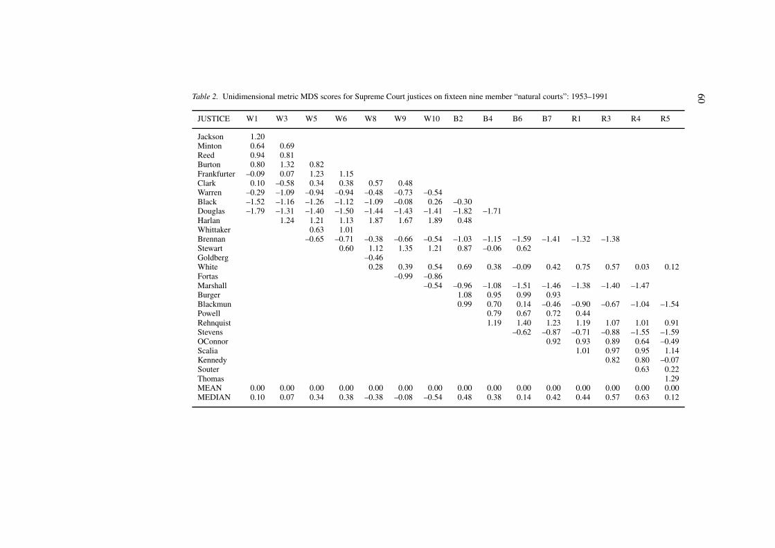
60Table 2. Unidimensional metric MDS scores for Supreme Court justices on fixteen nine member “natural courts”: 1953–1991

JUSTICE W1 W3 W5 W6 W8 W9 W10 B2 B4 B6 B7 R1 R3 R4 R5

Jackson 1.20Minton 0.64 0.69Reed 0.94 0.81Burton 0.80 1.32 0.82Frankfurter –0.09 0.07 1.23 1.15Clark 0.10 –0.58 0.34 0.38 0.57 0.48Warren –0.29 –1.09 –0.94 –0.94 –0.48 –0.73 –0.54Black –1.52 –1.16 –1.26 –1.12 –1.09 –0.08 0.26 –0.30Douglas –1.79 –1.31 –1.40 –1.50 –1.44 –1.43 –1.41 –1.82 –1.71Harlan 1.24 1.21 1.13 1.87 1.67 1.89 0.48Whittaker 0.63 1.01Brennan –0.65 –0.71 –0.38 –0.66 –0.54 –1.03 –1.15 –1.59 –1.41 –1.32 –1.38Stewart 0.60 1.12 1.35 1.21 0.87 –0.06 0.62Goldberg –0.46White 0.28 0.39 0.54 0.69 0.38 –0.09 0.42 0.75 0.57 0.03 0.12Fortas –0.99 –0.86Marshall –0.54 –0.96 –1.08 –1.51 –1.46 –1.38 –1.40 –1.47Burger 1.08 0.95 0.99 0.93Blackmun 0.99 0.70 0.14 –0.46 –0.90 –0.67 –1.04 –1.54Powell 0.79 0.67 0.72 0.44Rehnquist 1.19 1.40 1.23 1.19 1.07 1.01 0.91Stevens –0.62 –0.87 –0.71 –0.88 –1.55 –1.59OConnor 0.92 0.93 0.89 0.64 –0.49Scalia 1.01 0.97 0.95 1.14Kennedy 0.82 0.80 –0.07Souter 0.63 0.22Thomas 1.29MEAN 0.00 0.00 0.00 0.00 0.00 0.00 0.00 0.00 0.00 0.00 0.00 0.00 0.00 0.00 0.00MEDIAN 0.10 0.07 0.34 0.38 –0.38 –0.08 –0.54 0.48 0.38 0.14 0.42 0.44 0.57 0.63 0.12

61

Table 3. Ideological rank order of Supreme Court justices on fifteen nine member “naturalcourts” 1953–1991 (based on unidimensional non-metric MDS scores)

JUSTICE W1 W3 W5 W6 W8 W9 W10 B2 B4 B6 B7 R1 R3 R4 R5

Jackson 9

Minton 6 6

Reed 8 7

Burton 7 8 6

Frankfurter 4 5 8 8

Clark 5 4 5 6 7 7

Warren 3 3 3 3 3 3 3

Black 2 2 1 2 2 5 6 4

Douglas 1 1 1 1 1 1 1 1 1

Harlan 9 9 8 9 9 9 5

Whittaker 6 7

Brennan 4 4 5 4 4 2 2 2 2 1 1

Stewart 5 8 8 8 7 4 7

Goldberg 4

White 6 6 7 6 5 4 5 6 5 4 5

Fortas 2 2

Marshall 5 2 3 1 1 1 1 2

Burger 8 8 8 8

Blackmun 8 6 5 4 3 4 3 2

Powell 7 6 6 5

Rehnquist 9 9 9 7 6 9 7

Stevens 3 3 4 3 1 1

OConnor 7 7 6 6 3

Scalia 7 6 8 8

Kennedy 6 6 4

Souter 5 6

Thomas 9

have recoded the data so that negative numbers reflect positions on the left,while positive number reflect positions on the right (relative to members ofthat court). There is no absolute meaning to location of the zero point; it ismerely a centrist position relative to members of that court and has no largerideological meaning. Note also that the mean values of all justices are normedto sum to zero.

62

Table 4. Ideological rank order of Supreme Court justices on fifteen nine member “naturalcourts” 1953–1991 (based on unidimensional metric MDS scores)

JUSTICE W1 W3 W5 W6 W8 W9 W10 B2 B4 B6 B7 R1 R3 R4 R5

Jackson 9

Minton 6 6

Reed 8 7

Burton 7 9 7

Frankfurter 4 5 9 9

Clark 5 4 5 5 7 7

Warren 3 3 3 3 3 3 3

Black 2 2 2 2 2 5 6 4

Douglas 1 1 1 1 1 1 1 1 1

Harlan 8 8 8 9 9 9 5

Whittaker 6 7

Brennan 4 4 5 4 3 2 2 1 2 2 2

Stewart 6 8 8 8 7 4 6

Goldberg 4

White 6 6 7 6 5 4 5 6 5 4 5

Fortas 2 2

Marshall 3 3 3 2 1 1 1 2

Burger 9 8 8 8

Blackmun 8 6 5 4 3 4 3 2

Powell 7 7 6 5

Rehnquist 9 9 9 9 9 9 7

Stevens 3 3 4 3 1 1

OConnor 7 7 7 6 3

Scalia 8 8 8 8

Kennedy 6 7 4

Souter 5 6

Thomas 9

Tables 3 and 4 retabulate the numbers in Tables 1 and 2 in ordinal terms.Values range from 1 (most liberal) to 9 (most conservative), with values of 5those of the median justice. Cells indicating the median justice(s) are outlinedin bold. Comparison of Tables 3 and 4 shows that, in all of the courts exceptWarren 6 (where there is an interchange of the position of the median and aneighboring justice), the median justices identified by metric and non-metric

63

scaling models are in fact, identical, except for ties (Warren10) . Therefore,to simplify our discussion, we will henceforth refer only to the metric MDSestimates, since these estimates make somewhat finer distinctions among thelocations of the justices and also have a marginally higher explained variance.

One strong finding that can be gleaned from Table 4 is that the identity ofthe median justice is frequently shifting. Eleven of the 27 justices have beenthe median justice on at least one of the fifteen natural courts – all but twoonly once.14 One justice has thrice been median (Justice Clark), and one re-markable justice (Justice White) has been the pivotal justice for a substantialproportion of his career on the court, serving as a median justice on a totalof four different courts – two in the Burger era and two under Chief JusticeRehnquist.

Identifying the median justice as we do in Tables 3 and 4 allows us toidentify the ideological center of gravity of each of our natural courts. Overtime that center of gravity shifts from justices such as Clark and Frankfurter,to Justices Marshall, to Justice White, and then to more recently appointedjustices such as Powell, and later Justices O’Connor and Souter. In a relativelypolarized court, such as the one we now have, the views of the median justicecan be critical in determining outcomes on vital policy issues, as is arguablypresently the case for Justice O’Connor re affirmative action (Biskupic, 1997)and voting rights (Grofman, 1997).15 It does not take much knowledge of theSupreme Court to recognize that a court with Justice Frankfurter as medianjustice is a very different court from one where Justice Marshall plays thatrole.16

2.2.3. Has the overall ideology of the Court shifted rightward?While we lack a straightforward baseline model to determine if there is stat-istically significant shift over time in the location of individual justices,17 wecan get a clear sense of overall ideological shift in the Court by looking at thepatterns of judicial replacements. This allows us to get a measure of ideolo-gical movement “from the data” rather than by subjectively coding particularcases in left-right terms.

Table 5 shows the effects of judicial replacement by identifying the rank(ideological location) of the justice who is being replaced in the last fullcourt on which that justice served and the rank (ideological location) of thereplacement justice in the first full court on which that justice served. Thedifference between these ranks provides us a direct measure of the extent towhich replacements move the court in a given ideological direction.

The transformations shown in Table 5 are dramatic. After the first War-ren Court we see a steady leftward drift (with the biggest jump occurringwhen Justices Frankfurter and Clark are replaced by Justices Goldberg and

64

Table 5. Replacement effects on fifteen nine member “natural courts” 1953–1991 (based onunidimensional metric MDS ranks)

Court Replacement Position Replaced Position/ Difference

justice(s) rank on justice(s) rank on

first full last full

Court Court

served served

WAR 1 Warren x x x x

WAR3 Harlan 8 Jackson 9 –1

WAR5 Whittaker 6 Reed 7 –1

Brennan 4 Minton 6 –2

WAR6 Stewart 6 Burton 7 –1

WAR8 Goldberg 4 Frankfurter 9 –5

White 6 Whittaker 7 –1

WAR9 Fortas 2 Goldberg 4 –2

WAR10 Marshall 3 Clark 7 –4

BURG2 Burger 9 Warren 3 +5

Blackmun 8 Fortas 2 +6

BURG4 Rehnquist 7 Black 4 +3

Powell 7 Harlan 5 +2

BURG6 Stevens 3 Douglas 1 +2

BURG7 O’Connor 7 Stewart 6 +1

RENQ1 Scalia 8 Burger 8 0

RENQ3 Kennedy 6 Powell 5 +1

RENQ4 Souter 5 Brennan 2 +3

RENQ5 Thomas 9 Marshall 2 +7

Marshall, respectively). Every change during the Warren era after Warren3 is either a change in the direction of liberal ideas or neutral! But thencomes the first full Burger Court (Burger 2), reflecting a sharp right turn.That right turn continues. Every change during the Burger Court is a changein a conservative direction! Similarly, with the exception of the more or lesseven swap of Justice Scalia for Justice Burger, every change in the Rehnquistera is a change in a conservative direction, with the most dramatic effectsoccurring with the replacements of Justice Brennan by Justice Souter and, of

65

course, most dramatically, with the replacement of Justice Marshall by JusticeThomas! It does not take advanced statistics to see that these results are bothsubstantively and statistically significant.18

2.3. Comparisons with results of previous work

2.3.1. Locations of justices: Comparisons with Schubert (1974)Because the data analyzed by Schubert (1974) from 1946–1969 overlaps inpart with the time period of our study, and because he uses a version of MDSfor some of his analyses, we will provide direct comparisons for the naturalcourts found in both data sets.19 For Warren 1, our metric rank ordering fromleft to right is Douglas, Black, Warren, Frankfurter, Clark, Minton, Burton,Reed, Jackson; while for Schubert (1974: 135) it is Douglas, Black, Warren,Clark, Frankfurter, Jackson, Burton, Minton, Reed. All the differences, withthe exception of the switch between Jackson and Reed, occur as locationalswitches between proximate justices. For Warren 3 our ordering is identicalwith his. For Warren 5, Schubert gets an ordering of Black, Douglas, War-ren, Brennan, Frankfurter, Clark, Harlan, Whittaker, and Burton; while weget Douglas, Black, Warren, Brennan, Clark, Whittaker, Burton, Harlan, andFrankfurter. Here there are important differences in the results of the twomethods, especially with respect to the location of Frankfurter. For Warren6, Schubert’s smallest space analysis yields a near-degenerate solution, withfive justices at virtually identical locations at the rightmost pole and four at theleftmost pole (1974: 135); while our method yields a much clearer separationamong the positions of the justices (as does the non-metric analysis), butone which is otherwise identical to that given by Schubert in rankings. ForWarren 8 the two methods again get identical results. For Warren 9, the twomethods give identical rankings except for two inversions between proximatejustices: between Clark and White and between Warren and Fortas. For War-ren 10 we get Douglas, Fortas, a tie between Marshall, Warren, and Brennan,Black, White, Stewart, and Harlan; while Schubert (1974: 135) finds Douglas,Fortas, Marshall, a tie between Warren and Brennan, Stewart, Harlan, White,and Black. Clearly, for this court, we are agreeing on who is to the right andwho to the left, but not necessarily fully agreeing on relative location (at leaston the right). In four of the seven courts for which we can directly compareour work and that of Schubert (1974), we identify the same median justice. Inone instance (Warren 1 and Warren 5) we get an inversion between two prox-imate justices, and only in Warren 10 do our results differ significantly, buteven there the reason for the difference is simply that smallest space analysisplaces four justices very very close to one another but not in the same order asin our MDS analysis. The computer program Schubert (1974) uses reflects anearlier generation of technology and has a tendency to come up with solutions

66

in which not all justices have unique positions. This problem arises in a majorway in 20% of his one-dimensional solutions. Thus, in general, we regard ourresults as “cleaner”.

2.3.2. Replacement effects on the CourtWhen we look at replacement effects using Schubert’s one-dimensional smal-lest space results, we again find a dramatic shift leftward in the Warren Court,with seven of the eight shifts in a leftward direction.20 Moreover, Schubert’sdata, which go back further than ours, allows us to see what the effect was ofreplacing Justice Vinson with Justice Warren, namely a whopping - 6 (left-ward) shift in ideological ranks. This would suggest that, in the modern era,only the replacement of Justice Marshall by Justice Thomas had a greaterimpact on the ideological makeup of the Supreme Court.

The other work on replacement effects we have found tends to look only aspecific set of cases. But results are generally highly consistent with our own.For example, looking only at search and seizure cases, Segal (1985) findsevidence of a clear rightward shift during the Burger Court.

Baum (1992) offers one of the most sophisticated attempts to identifythe importance of replacement effects, especially as compared to changesin case content and changes in issue attitudes of continuing justices. His datais limited to civil liberties cases but he looks at a longer time period thanwe have. He finds (1992: 11–12) that “the decline in civil liberties supportbetween the early and late Vinson courts resulted entirely from membershipchange – a spectacular drop in support as the very liberal Frank Murphy andWiley Rutledge were succeeded by Tom Clark and Sherman Minton. . . .Similarly, the growth in civil liberties support in the 1956 and 1957 terms canbe attributed entirely to the arrival of two new justices, the more important byfar being William Brennan (Charles Whittaker was the other). . . .The growthin civil liberties support that created the later the Warren Court in the 1962–1964 period apparently derived overwhelmingly from the appointments ofByron White and Arthur Goldberg in 1962”.

While Baum (1992:13) finds changes between other natural courts arisingpartly from replacement and party from other effects, his overall conclusionis that “changes in the Court’s membership seems to account for a majorityof the voting change”.21 Moreover, when we compare the data in our Table 5with that in his Table 3 (1992: 13), we find that his conclusions about thedirectionality of change with respect to civil liberties over the period 1953–1985 are virtually identical to our findings for the entire set of cases beforeeach natural court over the same period. In particular, judged by his data onvoting on civil liberties cases, from 1953 to 1964 all replacement effects are

67

in a liberal direction, and from 1969–1985 all replacement effects are in aconservative direction.

2.4. Other issues

In this paper we have focused on a relatively limited set of judicial behaviorquestions such as the dimensionality of Supreme Court decision-coalitionsand the importance of judicial replacements. In doing so, we have only madeuse of voting data, not the content of opinions and not other information aboutinternal processes of the Court. While we make no claim that multidimen-sional scaling of court decisions is the only way, or even the most informativeway, to make sense of the decision processes of multi-judge courts, it is stilla natural question to consider in what ways our analyses might be misleading

First, while ideology is the natural way to explain the dimensional pat-terns we find in legislative roll-call data, some readers may have objected toour repeated use of the term “ideology” to characterize the attitudinal under-pinnings of judicial decision-making in the discussion above. If there existsa consistent patterning of judicial choices that is remarkably similar acrosscases, it might be the case that these similarities in voting alignments are dueto similarities in “jurisprudential philosophies”, rather than due to similaritiesin something like what is commonly thought of as “ideology”. Dimensionalscaling, per se, cannot allow us to choose between these two interpretations,and discussion of theories of jurisprudence and case-specific analyses wouldtake us well beyond the scope of the present paper.22 However, if the readerfinds herself uncomfortable with the use of the term “ideology” to referto the underpinnings of Supreme Court decision-making, s/he may simplysubstitute the phrase, “data that fits a Coombsian unfolding model”.23

Second, it might be argued that since justices might engage in strategicbehavior – including the decisions to engage in separate (or joint) concurringand dissenting opinions – that YES-NO roll-call votes can be limited or evenmisleading indicators of justices’ true attitudes. However, we do not regardthis claim as creating a major problem in interpreting our results. In ourview, the limitations of using roll call voting data as an indicator of judicialvalues are essentially no greater for courts than they are for legislators.24

For congress, evidence for strategic voting on the floor is very hard to comeby. Similarly, Segal (1997; 1998: 923) finds, “consistent with the attitudinalmodel, that the justices overwhelmingly engaged in rationally sincere be-havior”. For congress, analyses of roll-call voting patterns and coalitionalpatterns continue to be central in the study of topics such as the degree ofparty polarization (See e.g. Collie, 1988) and the representativeness of con-gressional committees (Krehbiel, 1990, 1991; Hall and Grofman, 1990).25 Inlike manner, considering the immense amount of effort that legal scholars

68

have put into analysis of the wellsprings of judicial decision-making, espe-cially that of the Supreme Court, it seems to us quite remarkable how far weget merely by thinking of justices as points along a line, with ideologicalproximity the best predictor (and a very good one!) of which coalitionalalliances will form.

Finally, we would note that no single study can do everything. By trackingchanges over time in the location of the median justice, we have identifiedchanges in the attitudinal “center of gravity” of the court, and we have shownhow pairwise replacement effects have either taken the court strongly in aliberal direction (during the Warren era) or strongly in a conservative dir-ection (during both the Burger and Rehnquist eras, through 1991).26 Ourresults, based on a different methodology, strongly support Baum’s (1992:22) finding that “presidential appointments appear to be the primary forcethat reshapes the decisions of the Supreme Court”.27 In sum, we see our workas establishing a basic schematic overview of nearly 40 years of court historyto serve as a springboard to more detailed analyses of judicial philosophy andjudicial choices and the changing dynamics of the Court that may come withthe appointment of new members, especially a new Chief Justice, and with theintroduction of new issues. Our work is based on a careful analysis of a mul-tidimensional scaling results for justices in nine member courts over a nearly40 year period. We have provided results disaggregated to natural courts aswell as evidence from pooled data. Unlike most other work in this area, wehave not restricted our analyses to subsets of the data selected because theydeal with some relatively narrowly defined type of policy question. Moreover,what we learn from MDS analyses of the Supreme Court has paralleled whatscholars such as Poole and Rosenthal (1997) have told us about the U.S.Congress.

Methodological appendix

Data

Using Spaeth’s (1993) codebook accompanying the ICPSR Supreme Courtdataset, the set of cases we analyze was initially screened by selecting dataset“cases” where his level of analysis variable ANALU = “ ” and his decisiontype variable DEC_TYPE = 1. We focus on “natural courts” with a substantialnumber of cases hears, since Courts with too few cases reduce the reliabilityof the MDS spatial estimates.

There were 23 natural courts during the period 1953–1991. Of these, sev-enteen were nine member courts. We report as the first number below thenumber of cases actually used for analyses of that natural court after we have

69

performed our screening; the second number is total number of cases in thedata set for that court before screening. Warren Court 1 (N = 48/65), con-sists of Justices Black, Burton, Clark, Douglas, Frankfurter, Jackson, Minton,Reed, and Warren. In Warren Court 2 (N = 36/39, omitted), Justice Jacksonleaves the court but is not yet replaced (this court has only eight members). InWarren Court 3 (N = 75/121), Justice Jackson is replaced with Justice Harlan.In Warren Court 4 (N = 26/43, omitted), Justice Minton is replaced withJustice Brennan. In Warren Court 5 (N = 116/161), Justice Reed is replacedwith Justice Whittaker. In Warren Court 6 (N = 291/342), Justice Burton isreplaced with Justice Stewart. In Warren Court 7 (N = 0/49, omitted), JusticeWhittaker is replaced with Justice White, but Frankfurter fails to serve on anyof the decisions in our reduced data set. In Warren Court 8 (N = 270/312),Justice Frankfurter is replaced with Justice Goldberg. In Warren Court 9 (N =161/197), Justice Goldberg is replaced with Justice Fortas. In Warren Court10 (N = 98/175), Justice Clark is replaced with Justice Marshall. In WarrenCourt 11 (N = 29/34, omitted), Justice Fortas steps down but is not yet re-placed (this court has only eight members). In Burger Court 1 (N = 56/70,omitted), Justice Warren is replaced with Justice Burger (this court has onlyeight members). In Burger Court 2 (N = 95/128), Justice Fortas is replacedwith Justice Blackmun. In Burger Court 3 (N = 18/18, omitted), JusticesBlack and Harlan leave but are not yet replaced. In Burger Court 4 (N =394/514), Justice Black and Harlan are replaced with Justices Rehnquist andPowell . In Burger Court 5 (N = 6/6, omitted), Justice Douglas leaves the courtbut is not yet replaced (this court has only eight members). In Burger Court6 (N = 569/772), Justice Douglas is replaced with Justice Stevens. In BurgerCourt 7 (N = 624/728), Justice Stewart is replaced with Justice O’Connor.In Rehnquist Court 1 (N = 132/145), Justice Burger is replaced with JusticeScalia. In Rehnquist Court 2 (N = 21/22, omitted ), Justice Powell departsbut is not yet replaced. In Rehnquist Court 3 (N = 303/378), Justice Powell isreplaced with Justice Kennedy. In Rehnquist Court 4 (N = 100/112), JusticeBrennan is replaced with Justice Souter. In Rehnquist Court 5 (N = 87/106),Justice Marshall is replaced with Justice Thomas.

Of the 17 nine-member courts, we omitted Warren Court 4, with only26 cases after data reduction, and Warren Court 7, with no cases after datareduction. We should note that Warren 7, though technically a nine-membercourt, was not a nine member court in practice, since Frankfurter, althoughformally still on the court, only participated in 8 of the 93 decisions. Theminimum number of cases in any of the natural courts we analyze is 48, inWarren 1.

Including cases with less than a full court might reduce the dimensionalityof our solution; thus the decision to exclude them is a conservative choice in

70

making a solution with low dimensionality less likely.28 We also analyze onlythose cases from this data set uniquely identified by case citation number,in which the Court heard oral argument and gave a formally decided fullopinion.29 Where it is used below, the term “case” refers to just these types ofcases. Note that all cases involving certiorari or cases with only memorandumopinions are excluded by the coding decisions we have made.30

Because we are focusing on affirmance or denial of the lower court de-cision, we do not require that cases have a majority opinion, as long asthe directionality of a decision is clear. Spaeth’s categorizations of justice’svoting behavior were binarized by recoding “voted with majority”, “regularconcurrence”, “special concurrence”, and “judgment of the court” as concur-rences and “dissent” as dissent. Cases where one or more Justice’s votes werecategorized as “jurisdictional dissent”, “dissent from a denial or dismissal ofcert”., and “non-participation”, (namely those for which full roll call datais not available) were also deleted from the data set. Spaeth identified somedecisions that he viewed as not being codeable in left-right terms.31 However,although our interest is in ideological scaling, we have not eliminated thosedecisions from the data set. Including cases that Spaeth did not see as code-able in left-right terms is another conservative choice because it makes it lesslikely that a unidimensional model will satisfactorily fit the data.

In our fifteen-court data set we have 4256 cases before data reductionand 3363 cases after data reduction. Because we have deliberately restrictedthe set of decisions we would analyze in a number of ways, it is natural toask how much of the data set has been excluded and would our results havebeen different if we had chosen a more inclusive strategy.32 First, we wouldemphasize that, even though we only look at 15 of the 23 natural courts,those courts include 93.8% (4256/4537) of the cases before reduction and94.6% (3363/3555) of the cases after reduction during the time period understudy. Second, a more inclusive strategy would not have significantly alteredour results. For example, comparisons between the one-dimensional MDSscalings reported below and additional analyses where both cases with lessthan full participation and cases involving certiorari decisions were includedshow almost no difference in average fit.33 Moreover, our choice of whichtypes of cases to include and which to exclude has minimal consequences foranalysis of the identity of the median justice.34

We would expect the fit of the MDS model to be greater on average for thedisaggregated than for pooled data. One likely source of multidimensionalityin the pooled data is the introduction of new issues confronting the courtsuch that the issue positions of justices with respect to these issues are notthe same as for the issues that had been previously been central. By focusingon single natural courts, we minimize this problem. Another likely source of

71

error (and thus potential imputed higher dimensions) is changes over time inthe issue locations of justices, i.e., even if the issues don’t change, the viewsof particular justices might. Ceteris paribus, the longer the time period overwhich we examine decisions of a sitting justice, the more likely is it thatthere will be some ideological drift in that justice’s position. For comparisonpurposes we pooled together the 15 data sets (yielding 3363 cases), computedsimple matching coefficients between each pair of the 27 justices that servedover this time period, and analyzed the resulting matrix as before with metricand non-metric MDS. The results were as expected. The r2 value was .79for the one-dimensional metric MDS solution, and .79 for the non-metricsolution as well. For the two-dimensional solutions we found r2 values of.91 for metric MDS and .90 for non-metric MDS. This is a drop of .05 to.06 in total r2from the average values for the individual natural courts of onedimensional and two-dimensional fit.

Finally, we examined what might be considered the “worst case” scenario,where the pooled data set subject to MDS was expanded in ways that might beexpected to introduce still further sources of error. We selected the formallydecided full opinion cases uniquely identified by case citation number (asbefore), but now included cases from all 23 courts (including the eight mem-ber courts), and left in those cases where there were less than nine justicesparticipating. (These are the cases where Spaeth coded the Justice’s vote as5 (non-participation), 7 (dissent from a denial or dismissal of certiorari ordissent from summary affirmation), or 8 (jurisdictional dissent).) This left anaggregated dataset of 4537 cases, which we then analyzed as above. Herethe fit is slightly worse, but not remarkably so. The r2 value was .75 for theone-dimensional metric MDS solution, and .75 for the non-metric solutionas well. For the two-dimensional solutions we recovered r2 values of .88 formetric MDS and .87 for non-metric MDS.

Even though the MDS fit for the pooled data is not that bad, our interest intracking justices over time lead us to prefer dealing with analyses of eachof the 15 natural courts, separately; moreover, the estimates of individuallocations are not as precise when we use the pooled data set.

2.5. Methods

We make no effort in this paper to provide a general mathematical descrip-tions of MDS techniques since these are available elsewhere (e.g., Kruskaland Wish, 1991), and MDS algorithms are now being included in most ad-vanced statistics program. MDS is closely related to the idea of Coombsianunfolding (Coombs, 1964). The unfolding model has been independentlydiscovered by scholars in different disciplines who often write in ignoranceof each other’s work. Coombs (1964) distinguished between I scales and J

72

scales. Coombsian J scales posit that we can locate both individuals andstimuli in the same metric space. An I scale is an individual’s preferenceordering of the stimuli and may be thought of as the J scale unfolded on theideal point of the individual, with only the rank order of the stimuli given inincreasing distance from the ideal point (Coombs, 1964). In one dimension,the set of Coombsian I scales that are consistent with a given CoombsianJ scale gives a form of what economists (Black, 1958; Arrow, 1961) call a“single-peaked” ordering. However, there may be some single-peaked order-ings that do not coincide with any Coombsian J scale because, although theordinality conditions required for a set of individual orderings to be single-peaked are satisfied, any proposed metric on the alternatives gives rise tological inconsistencies.

Generally, MDS techniques seek to optimize some objective functionof goodness (or badness) of fit between the observed proximities and thedistances between the points in the geometric configuration. The most com-monly used objective functions, STRESS 1 and STRESS 2 (Kruskal 1964a,1964b) are actually badness of fit measures, as is Young’s S-STRESS. Whilethe results we report were done using SYSTAT 5.0, a program which minim-izes the value of Kruskal’s STRESS 1, as an added precaution, the resultswere replicated using SPSS for Windows, which minimizes Young’s S-STRESS. Ordinal results from the two programs were virtually identical, withonly a few pairwise reversals of the location of proximate justices in someof the natural courts. Moreover, differences found in ordinal rankings invari-ably involved justices whose metric locations were virtually indistinguishablefrom one another. The correlations between the one-dimensional solutions ofthe two programs were .99 for both the metric and the non-metric solutions,and the same was true for the two dimensional solutions. Because the resultsof the two methods were so close, we have only reported results from theSYSTAT runs.

Largely following Poole and Rosenthal (1997), we focus on explainedvariance. The explained variance is the square of correlation between the rawdata (i.e., for each pair of justices on a given natural court, the proportion ofcases in which those two justices vote the same) and the MDS-recoveredinter-justice (paired) distances. In the MDS literature, so-called “Sheparddiagrams “ are commonly used to display the scattergram between the rawdata and the MDS distance estimates (Kruskal and Wish, 1991). We are re-porting the square of the correlation that would be found for the data in suchscattergrams. This value is, we believe, directly comparable to the explainedvariance reported in the work of Poole and Rosenthal (1991a, b). We have notreported values for the various stress measures common in the MDS literature

73

(see e.g. Kruskal and Wish, 1991 and discussion above) because the explainedvariance measures are more readily interpretable.35

Notes

1. The classic early works on congressional roll-call voting analysis are Turner (1951) andMacRae (1958). The methodological underpinnings of this early behavioral work are laidout in MacRae (1970). Similar methods have been applied to legislatures outside the U.S.(see e.g., MacRae, 1967). What is unquestionably the most important recent scholarshipin this area has been by Keith Poole and Howard Rosenthal (see Poole and Daniels, 1985;Poole and Rosenthal, 1984, 1991a, 1991b, 1997). The Poole and Rosenthal work reflectsmajor technical advances over the work of the 60s and 70s on roll-call voting.

2. While “legal realism” got its start among lawyers (see e.g., Frank, 1949), it has largelybeen political scientists such as Glendon Schubert (1959, 1964, 1965, 1974), and HaroldSpaeth (1963a, 1963b, 1979), and their students and successors (e.g., Spaeth and Peterson,1971; Rohde and Spaeth, 1976; Spaeth and Brenner, 1990; Hagle and Spaeth, 1992; Segaland Spaeth, 1993), who, beginning in the late 1950s, have provided the empirical evidenceto buttress a claim that the policy attitudes of Supreme Court justices serves as the prin-cipal determinant of their voting behavior. The locus classicus for the modern empiricalstudy of the Supreme Court, however, is Pritchett (1948) which viewed the Court as apolitical institution, looked at the social values of justices, and introduced bloc analysisas a tool for analysis of court decisions. Other important early work was done by Ulmer(1960, 1970, 1973a, 1973b, 1974)– some of it arguing for the importance of judge’s socialbackground.

3. The literature on Supreme Court decision-making is too voluminous to review in capsuleform, but numerous articles and books focusing on the Supreme Court are cited in thetext below and a useful, although now dated, review is found in Ryan and Tate (1980);important general treatments of judicial behavior and public law include Murphy andTanenhaus (1972), Gibson (1983), Shapiro (1993), and Baum (1997). Reviews of thejudicial behavior literature on trial and lower appellate courts, respectively, are found inJacob (1991) and Gibson (1991).

4. Multidimensional scaling (hereafter MDS) is a class of techniques designed to reduce amatrix of proximities to a geometrical configuration of points lying in some number ofdimensions in such a way that the distances dij between the points are related in somefashion to the proximities δij. MDS is based on capturing underlying dimensions in termsof what is called Coombsian unfolding (Coombs, 1964). There are both metric and non-metric versions of MDS (see e.g., Torgerson, 1958; Shepherd, 1962a, l962b; Kruskal,1964a, l964b; Shepherd, Romney and Nerlove, 1973a; Kruskal and Wish, 1991). Thelatter may be used where proximity between stimuli is not specified in metric terms andonly ordinal information about relative closeness is known.

5. Cf. Feld and Grofman (l988).6. See van Schuur and Kiers (1994) and Brazill and Grofman (2000).7. In contrast, there is a long tradition of MDS use in disciplines such as mathematical

anthropology and mathematical psychology (see e.g., Shepherd, Romney and Nerlove,1972b; Carroll and Wish, 1974; Kruskal and Wish, 1991).

8. This data set, “United States Supreme Court Judicial Database: 1953–1991 Terms”, wasmade available to us through ICPSR (ICPSR 9422 4th Release, May 1993).

74

9. See Appendix for methodological details.10. The choice of metric scaling instead of non-metric scaling has only limited effect on the

general configuration of points in most cases. As we shall see, the differences betweenmetric and non-metric MDS results proved unimportant for our analyses of SupremeCourt data. For more detailed discussion of differences between metric and non-metricMDS see Kruskal and Wish (1991).

11. See methodological appendix for further details (cf. Poole and Rosenthal, 1991a, b; 1997).12. We would emphasize that we would never expect to get a perfect scale pattern. As Poole

and Rosenthal (1997:7) observe for congressional roll-voting analyses: “Allowance mustbe made for errors”. We can make such an allowance via “a probabilistic model of voting.“ Errors, however, should not be randomly distributed. In particular, errors should be mostcommon among legislators who are located near the “cut-point” between any proposaland the status quo reversion point that obtains if that proposal fails to pass. MDS finds thedimensional structure that best fits the data, and allows for mistakes.

13. The results we get when we report ordinates on the first dimension of the two-dimensionalMDS solutions are so similar to those for the unidimensional solutions that we do notbother to present them. Using SYSTAT, the correlations between the first dimension ofthe two dimensional solution and the one dimensional solution are .98 for non-metricMDS and .99 for metric MDS.

14. Recall that there is one tie for median.15. For a much more general perspective on Justice O’Connor’s influence on the Court see

Maveety (1996).16. However, we would repeat the caution of Blasecki (1990) not to confuse a centrist location

with (pivotal) influence on the Court. Some justices may be influential even though farfrom centrist, and some centrist justices may have little persuasive influence on theirfellows and, if there are several justices who are generally centrist, there is no guaranteethat the justice who is most often median is also the one with the greatest bargainingpower/influence on the final shape of the opinion.

17. Our evidence for a genuine ideological shift on the part of Justice Blackmun relies onthe “inter-ocular” test as it applies to Table 4 and not on any explicit statistical model.We hope in future work to explore the possibility of developing such a baseline statisticalmodel.

18. Indeed, the probability that we could get a sequence of eight values less than or equal tozero (change in the liberal direction) being followed by ten values greater than or equal tozero (change in the conservative direction) by chance alone is effectively zilch!

19. For reasons discussed below, we will only deal with the analyses done by Schubert (1974)using “smallest space analysis”, which is a form of MDS. Also, to maximize comparab-ility, we will only look at the one-dimensional solutions he found. We will not try tocompare our scaling of justices’ locations with those in the other detailed analysis ofSupreme Court data using smallest scale analysis, Spaeth and Peterson (1971), becausethat work focuses on comparisons of voting patterns in eleven different subsets of the civilliberties cases before the Warren Court in 1960–64 (Warren 8).

20. Only the replacement of Jackson by Harlan would not be scored as a leftward shift if weused the results of Schubert’s one dimensional smallest space analysis.

21. Later in the article, however, after reviewing data on the behavior of individual justicesover time, Baum (1992: 19) does modify this conclusion somewhat, by placing more equalemphasis on change in the attitudes of continuing justices as a source of change for theCourt as a whole. On balance, Baum (1992) aims for a nuanced portrait of the variousinfluences that create voting differences on the Court over time.

75

22. Perhaps the most sophisticated attempt to develop an empirically testable comparison ofcompeting theories of jurisprudence is Spaeth and Segal (1999), which focuses on staredecisis, and offers analysis of both voting patterns and the legal content of opinions.

23. But, if we find a pervasive unidimensionality that cuts across all cases, and if other schol-ars who have examined the substance of particular rulings find that justices whom ourscaling would classify as conservative at some point in time are, for example, willing tooverturn or emasculate policies favored by liberals of that time period (e.g., affirmativeaction), while sustaining policies generally favored by conservatives of that time period(e.g., anti-sodomy laws), then characterizing justices’ attitudes in the same way that wemight characterize the attitudes of legislators does not seem unreasonable. (Cf. “If it lookslike a duck and quacks like a duck, maybe it is a duck”.) For more on this debate from apolitical science point of view see e.g., Spaeth and Teger, 1982; Adamany , 1991; Brisbin,1996; Songer and Lindquist, 1996, and the references cited therein.

24. Certainly, any student of congress would find it completely uncontroversial to say thatwe cannot fully understand congress without a study of its internal structure (consider,for example the classic work of Shepsle, 1979 on committee structure, or the recent workof Hall, 1996 on committee and subcommittee influence), or without understanding theinterplay between congress and the president. It is equally uncontroversial to observe thata focus on who opposes and who supports a bill may lead us to neglect the actual policycontent of bills (as well as details of impact that may be “lost in the fine print”.) Similarly,dating back at least as far as Riker (1958) congressional scholars have been sensitized tothe potential for strategic calculations by members of congress. None of these concernsis incompatible with a view, which sees legislator ideology as a major determinant oflegislative voting. (cf. Gillman and Clayton, 1999)

25. Similarly, while a focus on roll-call voting leaves out some of the most important aspectsof judicial decision-making, namely the actual legal precedents and reasoning of the vari-ous opinions, legislative roll-call voting data analyses tell us nothing about the crucialquestion of what the bills that pass (or fail) actually contain.

26. We should also note, however, that, for both legislators and justices the specific policycontent of what is liberal and what is conservative may change over time (see e.g., Pooleand Rosenthal, 1997).

27. Similarly, Poole and Rosenthal (1991a: 228) conclude that changes in congressional vot-ing patterns have “occurred almost entirely through the process of replacement of retiringor defeated legislators with new members”.

28. Also, we did not wish to artificially inflate the similarity between those justices who mayhave simply failed to participate in some number of particular cases.

29. It should be noted that cases decided “on the merits” are rare, and cases with full signedwritten opinions are rarer, still In the 1994–95 term, the Court had 2526 cases on itsdockets [excluding the 5,574 in forma pauperis petitions from indigents seeking reversalsof their convictions] and disposed of the vast bulk of them. But of the many cases handledby the Court, “it decided only 160 on the merits, with full signed, written opinions handeddown in 91 cases. . . . the remainder being disposed of either per curiam, or by memor-andum orders (e.g., “affirmed”, “reversed”, “dismissed”, or “vacated”.)” (Abraham, 1998:197). However, the relatively small set of cases decided on the merits with signed writtenopinions are the precedent setting cases which are the lifeblood of jurisprudential analysis.

30. It might be argued that the decision coalitions in such cases might differ in substantiallysignificant ways from other cases before the Court.

76

31. In the fifteen-court data set there are 3,363 cases (after reduction) , but of these there wereonly a relatively small number (28) that Spaeth viewed as not being codeable in left-rightterms.

32. Several of our decisions as to which cases to exclude (e.g., the decision to exclude casesinvolving certiorari and the decision to exclude multiple decisions arising from a singlecase) were based in large part on suggestions of an anonymous referee of another (related)paper by the present authors. However, we take full responsibility for the coding choiceswe have made.

33. The average absolute difference between fit scores (squared multiple r) for the unidi-mensional solution to the larger as compared to the reduced data set was .045 (standarddeviation = .053) for non-metric MDS and .031 (standard deviation = .041) for the metricMDS scalings. Neither data set fit significantly better than the other. The average differ-ence between fit scores (squared multiple r) for the unidimensional solution to the largeras compared to the reduced data set was a minuscule .004 (standard deviation = .07) fornon-metric MDS and .006 (standard deviation = .052) for the metric MDS scalings.

34. In none of the comparisons with alternative data sets we performed, did the identity ofmore than one of the fifteen median justices change, although in some instances we alsogot additional ties.

35. A heuristic often employed is to examine the scree plot, a graph of the mean varianceexplained level for solutions of various dimensionalities (m = 1,2,3,. . . ). In theory, thereshould be an elbow in the plot marking the “true” underlying dimensionality. That is, vari-ance explained should increase rapidly until the appropriate dimensionality is reached andthen the plot should gradually flatten out, as the “additional” dimensions reflect mainlynoise. (Sometimes “stress reduction” rather than “variance explained” is used as the basisfor a decision about dimensionality.) We have not bothered to present such a graph here.

References

Abraham, H.J. (1998). The judicial process: An introductory analysis of the Courts of theUnited States, England and France. New York: Oxford University Press.

Adamany, D. (1991). The Supreme Court. In J.B. Gates and C.A. Johnson (Eds.), TheAmerican Courts: A critical assessment, 5–33. Washington, DC: CQ Press.

Arrow, K. (1961). Social choice and individual values (second edition). New York: Wiley.Baum, L. (1992). Membership change and collective voting change in the United States

Supreme Court. Journal of Politics 54: 3–24.Baum, L. (1997). The puzzle of judicial behavior. Ann Arbor, MI: University of Michigan

Press.Black, D. (1958). The theory of committees and elections. Cambridge: Cambridge University

Press.Blasecki, J.L. (1990). Justice Lewis F. Powell: Swing voter or staunch conservative? Journal

of Politics 52: 530–547.Biskupic, J. (1997). A justice in the spotlight: O’Connor’s vote could be crucial in one of the

Supreme Court’s most closely watched cases. Washington Post National Weekly Edition(October 13): 29.

Brazill, T.J. and Grofman, B. (2000). Factor analysis vs. MDS; Binary choice roll-call vot-ing and the U.S. Supreme Court. Presented at the Society for Cross-Cultural ResearchConference, February 25, 2000, New Orleans, LA.

77

Brisbin, R.A. (1996). Slaying the dragon: Segal, Spaeth and the function of law in SupremeCourt decision making. American Journal of Political Science 40: 1004–1017.

Carroll, J.D. and Wish, M. (1974). Multidimensional perceptual models and measurementmethods. In E.C. Carterette and M.P. Friedman (Eds.), Handbook of perception, Vol. II.,391–447. New York: Academic Press.

Collie, M. (1988). Universalism and the parties in the U.S. House of Representatives.American Journal of Political Science 32: 865–883.

Coombs, C. (1964). A theory of data. New York: Wiley.Feld, S.L. and Grofman, B. (1988). Ideological consistency as a collective phenomenon.

American Political Science Review 82: 64–75.Frank, J. (1949). Courts on trial: Myth and reality in American justice. Princeton: Princeton

University Press.Gibson, J. (1983). From simplicity to complexity: The development of theory in the study of

judicial behavior. Political Behavior 5: 7–49.Gibson, J. (1991). Decision-making in appellate Courts. In J.B. Gates and C.A. Johnson (Eds.),

The appellate Courts: A critical assessment, 255–278. Washington, D.C.: CQ PressGillman, H. and C.W. Clayton. (1999). Beyond judicial attitudes: Institutional approaches to

Supreme Court decision-making. In C.W. Clayton and H. Gillman (Eds.) (1989). SupremeCourt decision-making: New institutionalist approaches. Chicago: University of ChicagoPress.

Grofman, B. (1997). The Supreme Court, the Voting Rights Act, and minority representation”.In A. Peacock (Ed.), Affirmative action and representation: Shaw v. Reno and the futureof voting rights, 173–199. Durham NC: Carolina Academic Press.

Hagle, T. and H.J. Spaeth. (1992). The emergence of a new ideology: The business decisionsof the Burger Court. Journal of Politics 54: 120–134.

Hall, R.L. (1996). Participation in Congress. New Haven: Yale University Press.Hall, R.L. and Grofman, B. (1990). The committee assignment process and the conditional

nature of committee bias. American Political Science Review 84: 1149–1166.Jacob, H. (1991). Judicial decision-making in trial courts. In J.B. Gates and C.A. Johnson

(Eds.), The appellate Courts: A critical assessment, 213–233. Washington, D.C.: CQPress.

Krehbiel, K. (1990). Are congressional committees composed of preference outliers? Amer-ican Political Science Review 84: 149–163.

Krehbiel, K. (1991. Information and legislative organization. Ann Arbor, MI: University ofMichigan Press.

Kruskal, J.B. (1964a). Multidimensional scaling by optimizing goodness of fit to a nonmetrichypothesis. Psychometrika 29: 1–27.

Kruskal, J.B. (1964b). Nonmetric multidimensional scaling: A numerical example. Psycho-metrika 29: 115–129.

Kruskal, J.B. and Wish, M. (1991). Multidimensional scaling (Sage University Series onQuantitative Applications in the Social Sciences. Number 7): Beverly Hills and London:Sage Publications.

MacRae, D., Jr.(with the collaboration of F.H. Goldner). (1958). Dimensions of congressionalvoting: A statistical study of the House of Representatives in the eighty-first Congress.Berkeley: University of California Press.

MacRae, D. (1967). Parliament, parties, and society in France, 1946–1958. New York: St.Martin’s Press.

MacRae, D. (1970). Issues and parties in legislative voting: Methods of statistical analysis.New York: Harper & Row.

78

Maveety, N. (1996). Justice Sandra Day O’Connor: Strategist on the Supreme Court. Lanham,MD: Rowman and Littlefield.

Murphy, W.F. and Tanenhaus, J. (1972). The study of public law. New York: Random House.Poole, K.T. and Daniels, R.S. (1985). Ideology, party and voting in the U.S. Congress, 1959-

1980. American Political Science Review 79: 373–399.Poole, K.T. and Rosenthal, H. 1984. The polarization of American politics. Journal of Politics

46: 1061-1079.Poole, K.T. and Rosenthal, H. (1991a). Patterns of congressional voting. American Journal of

Political Science 35: 228–278.Poole, K.T. and Rosenthal, H. (1991b). On dimensionalizing roll call votes in the United States

congress. American Political Science Review 85: 955–960.Poole, K.T. and Rosenthal, H. (1997). Congress: A political-economic history of roll call

voting. New York: Oxford University Press.Pritchett, C.H. (1948. The Roosevelt court: A study in judicial politics and values, 1937–1947.

New York: The Macmillan Company.Riker, W. (1958). The paradox of voting and congressional rules for voting on amendments.

American Political Science Review 52: 349–366.Rohde, D.W. and Spaeth, H.J. (1976). Supreme Court decision-making. San Francisco: W.H.

Freeman.Ryan, J.P. and Tate, C.N. (1980). The Supreme Court in American politics: Policy through

law, 2nd Edition. Washington, D.C.: American Political Science Association.Schubert, G. (1959). Quantitative analysis of judicial behavior. Glencoe, Illinois: Free Press.Schubert, G. (Ed.) (1964). Judicial behavior: A reader in theory and research. Chicago: Rand-

McNally.Schubert, G. (1965). The judicial mind. Evanston: Northwestern University Press.Schubert, G. (1974). The judicial mind revisited. London: Oxford University Press.Segal, J. (1984). Predicting Supreme Court cases probabilistically: The search and seizure

cases, 1962–1981. American Political Science Review 78: 891–900.Segal, J.A. (1985). Measuring change on the Supreme Court: Examining alternative models.

American Journal of Political Science 29: 461–479.Segal, J.A. (1997). Separation of power games in the positive theory of Congress and courts.

American Political Science Review 91: 28–44.Segal, J.A. (1998). Correction to separation of power games in the positive theory of Congress

and courts. American Political Science Review 92: 923–926.Segal, J.A. and Spaeth, H. (1993). The Supreme Court and the attitudinal model. New York:

Cambridge University Press.Shapiro, M. (1993). Public law and judicial politics. In A.W. Finifter (Ed.), Political science:

The state of the discipline, II, 365–381. Washington, D.C.: American Political ScienceAssociation.

Shepard, R.N. (1962a). Analysis of proximities: Multidimensional scaling with an unknowndistance function, I. Psychometrika 27: 125–140.

Shepard, R.N. (1962b). Analysis of proximities: Multidimensional scaling with an unknowndistance function, II. Psychometrika 27: 219–246.

Shepard, R.N, Romney, A.K. and Nerlove, S.B. (Eds.) (1972a). Multidimensional scaling,Volume I: Theory. New York: Seminar Press.

Shepard, R.N, Romney, A.K. and Nerlove, S.B. (Eds.) (1972b). Multidimensional scaling,Volume II: Applications in the behavioral sciences. New York: Seminar Press.

Shepsle, K. (1979). Institutional arrangements and equilibrium in multidimensional votingmodels. American Journal of Political Science 23: 27–59.

79

Songer, D.R. and Lindquist, S.A. (1996). Not the whole story: The impact of justices’values on Supreme Court decision-making. American Journal of Political Science 40:1049–1063.

Spaeth, H.J. (1963a). An analysis of judicial attitudes in the labor relations decisions of theWarren Court. Journal of Politics 25: 290–311.

Spaeth, H.J. (1963b). Warren Court attitudes toward business: The ‘B’ scale. In G. Schubert(Ed.), Judicial decision-making. New York: Free Press.

Spaeth, H.J. (1979). Supreme Court policy making: Explanation and prediction. San Fran-cisco: W.H. Freeman.

Spaeth, H.J. (1993). Codebook: United States Supreme Court judicial database: 1953–1991terms. Ann Arbor, MI: International Consortium for Political and Social Research (ICPSR9422, 4th Release, May).

Spaeth, H.J. and Brenner, S. (1990). Studies in Supreme Court behavior. New York: Garland.Spaeth, H.J. and Peterson, D.J. (1971). The analysis and interpretation of dimensionality: The

case of civil liberties decision-making. Midwest Journal of Political Science 15: 415–441.Spaeth, H.J. and Segal, J.A. (1999). Majority rule or minority will: Adherence to precedent on

the United States Supreme Court. New York: Cambridge University Press.Spaeth, H.J. and Teger, S. (1982). Activism and restraint: A cloak for the justices’ policy

preferences. In S.C. Halpern and C.M. Lamb (Eds.), Supreme Court activism and restraint.Lexington, MA: Lexington Books.

Torgerson, W.S. (1958). Theory and methods of scaling. New York: Wiley.Turner, J. (1951). Party and constituency: Pressures on Congress. Baltimore: Johns Hopkins

Press.Ulmer, S.S. (1960). The analysis of behavior patterns in the Supreme Court of the United

States. Journal of Politics 22: 429–447.Ulmer, S.S. (1970). Dissent behavior and the social background of Supreme Court justices.

Journal of Politics 32: 580–598.Ulmer, S.S. (1973a). The longitudinal behavior of Hugo Lafayette Black: Parabolic support

for civil liberties, 1937–1971. Florida State University Law Review 1: 131–153.Ulmer, S.S. (1973b). Social background as an indicator to the votes of Supreme Court justices

in criminal cases, 1947–1956. American Journal of Politics 17: 622–630.Ulmer, S.S. (1974). Dimensionality and change in judicial behavior. In J.F. Herndon and J.L.

Bernd (Eds.), Mathematical applications in political science, VII, 40–67. Charlottesville,VA: University Press of Virginia.

Van Schuur, W.H. and Kiers, H.A.L. (1994). Why factor analysis often is the incorrect modelfor analyzing bipolar concepts and what model to use instead. Applied PsychologicalMeasurement 18: 97–110.