Identifying keystone trophic groups in benthic ecosystems: Implications for fisheries management

(This is a sample cover image for this issue. The actual cover is not yet available at this time.)

This article appeared in a journal published by Elsevier. The attachedcopy is furnished to the author for internal non-commercial researchand education use, including for instruction at the authors institution

and sharing with colleagues.

Other uses, including reproduction and distribution, or selling orlicensing copies, or posting to personal, institutional or third party

websites are prohibited.

In most cases authors are permitted to post their version of thearticle (e.g. in Word or Tex form) to their personal website orinstitutional repository. Authors requiring further information

regarding Elsevier’s archiving and manuscript policies areencouraged to visit:

http://www.elsevier.com/copyright

Author's personal copy

Ecological Indicators 25 (2013) 133–140

Contents lists available at SciVerse ScienceDirect

Ecological Indicators

jo ur nal homep age: www.elsev ier .com/ locate /eco l ind

Identifying keystone trophic groups in benthic ecosystems: Implications forfisheries management

Marco Ortiza,∗, Richard Levinsb, Leonardo Camposa,e, Fernando Berriosa,e, Fernando Camposa,Ferenc Jordánc, Brenda Hermosilloa,e, Jorge Gonzaleza,e, Fabián Rodriguezd

a Instituto Antofagasta, Instituto de Investigaciones Oceanológicas, Facultad de Recursos del Mar, Universidad de Antofagasta, P.O. Box 170, Antofagasta, Chileb Department of Global Health and Population, Harvard School of Public Health, Harvard University, 665 Huntington Avenue, Boston, MA 02115, USAc The Microsoft Research – University of Trento Centre for Computational and Systems Biology, Piazza Manifattura 1, Rovereto, TN, Italyd Laboratorio de Ecosistemas Marinos y Acuicultura (LEMA), Departamento de Ecología, CUCBA, Universidad de Guadalajara, Carretera Guadalajara-Nogales Km. 15.5, Las AgujasNextipac, Zapopan, 45110, Jalisco, Mexicoe Programa de Doctorado en Ciencias Aplicadas, Mención Sistemas Marinos Costeros, Facultad de Recursos del Mar, Universidad de Antofagasta, Antofagasta, Chile

a r t i c l e i n f o

Article history:Received 26 June 2012Received in revised form 15 August 2012Accepted 28 August 2012

Keywords:Keystone species complexMultispecies modellingCoastal ecosystemsSE Pacific

a b s t r a c t

Many species inhabiting the benthic marine ecosystems of the central and northern Chilean coast havebeen intensively harvested and this exploitation has increased considerably in recent years. Despite thisharvest pressure, few studies have attempted to establish a more holistic, systems-based managementplan. On the contrary, research continues to rely on population models in which the species of interestare isolated from their ecological context. This work offers several keystone indices in order to helpmultispecies fisheries management. The indices used are: (1) functional indices based on steady-state anddynamic trophic models; (2) structural indices based on bottom-up and top-down control mechanisms;and (3) qualitative keystone species indices using loop models (mixed control). The quantitative trophicmodels were constructed using Ecopath with Ecosim (EwE; v. 5.0) software, and the qualitative modelwas analysed using Loop Analysis. All models describe the interactions of the most representative speciesand functional groups inhabiting the benthic ecosystems of Tongoy Bay, La Rinconada Marine Reserve(Antofagasta Bay), and the kelp forest of Mejillones Peninsula (Antofagasta). Even though our results onlyrepresent the short-term dynamics of these systems, we have found keystoneness properties of severalspecies and functional groups, including primary producers, herbivores, and top predators. Despite thiswide variability of groups, we detected a different core set of species or functional groups, each of whichcontained prey–predator and plant–herbivore relationships. Because the traditional keystone conceptof a single species is difficult to apply, we suggest shifting away from this view towards a more holisticalternative such as that of a keystone species complex. This kind of approach would facilitate the designand assessment of sustainable management strategies for ecological marine ecosystems. Despite theecological relevance of our results, further experimental studies and modelling using other theoreticalframeworks should be performed.

© 2012 Elsevier Ltd. All rights reserved.

1. Introduction

Ever since Paine (1969) introduced the concept of keystonespecies to ecology, it has been the “cornerstone” for the devel-opment of numerous investigations in different communities andecosystems (Mills et al., 1993; Power et al., 1996), especially givenits direct and immediate use in the design and application of con-servation management programs (Payton et al., 2002). Of all thedefinitions proposed for keystone species, the most widespreadand the simplest was given by Power et al. (1996): “a species

∗ Corresponding author.E-mail address: [email protected] (M. Ortiz).

whose effect is large, and disproportionately large relative to its abun-dance”. Although the concept seems to be sufficiently clear, itsdetermination in communities and ecosystems is not, since thisrequires observations and studies that incorporate different spatio-temporal scales, levels of organization, and taxonomic groups(Power et al., 1996; Libralato et al., 2006).

Although numerous studies based on field experiments havequantified the strength of interactions by evaluating the impactspropagated on remainder species when the abundance of onespecies in a community changes (Paine, 1992; Berlow, 1999), thesestudies necessarily focused on a few species, excluding other “unin-teresting” species from the experiment and possibly causing aninevitable bias in the identification of keystone species (Wootton,1994; Libralato et al., 2006). Likewise, other external factors (i.e.,

1470-160X/$ – see front matter © 2012 Elsevier Ltd. All rights reserved.http://dx.doi.org/10.1016/j.ecolind.2012.08.020

Author's personal copy

134 M. Ortiz et al. / Ecological Indicators 25 (2013) 133–140

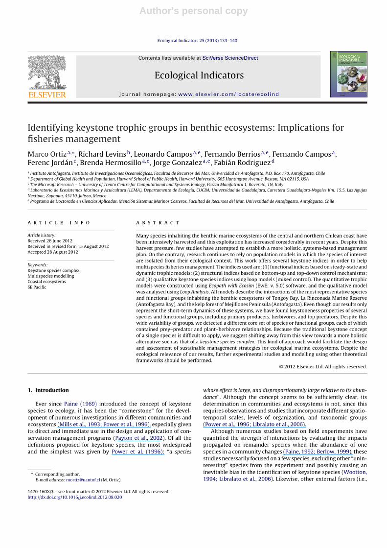
Fig. 1. Locations of the study areas in central and northern Chile: (1) Tongoy Bay, (2) La Rinconada Marine Reserve, and (3) the Mejillones Peninsula kelp forest.

level of exposure to coastal waves, environmental heterogene-ity, harvest) may cause the density of the species of interest tovary in different habitats, thereby hindering the necessary repli-cation of studies and the determination of keystoneness. Finally,some purely experimental studies (Pace et al., 1999) have omit-ted the propagation of higher-order effects – which are bufferedalong some pathways and amplified along others – despite the rec-ognized importance of this phenomenon (Wootton, 1994; Patten,1997; Yodzis, 2001).

Many studies have suggested characterizing the role that dif-ferent species play in their ecological systems by using differentnetwork indices (Jordán et al., 1999, 2007; Dunne et al., 2002;Luczkovich et al., 2003; Jordán and Scheuring, 2004; Allesina andBodini, 2005; Brose et al., 2005; Eklöf and Ebenman, 2006; Libralatoet al., 2006). Such multispecies modelling offers a complemen-tary way to deal with some of the limitations in the experimentalidentification of key groups. Quantitative trophic models per-mit estimations of the strength of interactions between modelspecies or functional groups by identifying the presence of keystonespecies, which occupy key positions in the networks (Jordán et al.,1999; Jordán and Scheuring, 2004). Keystoneness can also be deter-mined using qualitative loop models, in which case, the key positionof a species is a consequence of changes in its self-dynamics, mod-ifying the balance (prevalence) of positive and negative feedbacksand, thus, the local stability of the network.

Over the last few years, the multispecies modelling approachhas gained ground due to growing interest in the evaluation, quan-tification, and prediction of the changes that fisheries produce in

an ecosystem’s properties (Hall, 1999a,b; Robinson and Frid, 2003;Hawkins, 2004; Pikitch et al., 2004; Francis et al., 2007; Scotti et al.,2007; Crowder et al., 2008). Thus, multispecies models could beused for pre-screening, determining the core set of variables thatshould be considered in subsequent field experiments.

The aim of this work is to use pre-screening to identify keystonespecies based on: (1) functional indices using quantitative models(using EwE v. 5.0), (2) structural indices including bottom-up andtop-down control mechanisms, and (3) qualitative indices based onLoop Analysis (mixed control). All trophic models represent inter-specific relationships (prey–predator) taking place in the benthiccommunities of Tongoy Bay (Ortiz and Wolff, 2002a), La RinconadaMarine Reserve (SE Pacific coast) (Ortiz et al., 2010), and the kelpforest of Mejillones Peninsula (Antofagasta) (Ortiz, 2008a), all ofwhich are intensively exploited. The identification of keystonenessin these benthic networks would complement the existing infor-mation describing other attributes of such ecosystems (Ortiz andWolff, 2002a; Ortiz, 2008b, 2010; Ortiz et al., 2010; Ortiz and Levins,2011), thereby contributing to both conservation ecology and thedesign and implementation of sustainable multispecies fisheriesmanagement.

2. Materials and methods

2.1. Study areas

Three study areas are used herein. (1) Four habitats weremodelled in Tongoy Bay: seagrass meadows at depths of 0–4 m;

Author's personal copy

M. Ortiz et al. / Ecological Indicators 25 (2013) 133–140 135

sand-gravel between 4 and 10 m; sand between 10 and 14 m, andmud bottoms at >14 m depth (Fig. 1). (2) La Rinconada MarineReserve is located in the northern part of Antofagasta Bay (Mejil-lones Peninsula, Chile). At depths of 8–15 m, sand and graveldominate the physical benthos and two ecological subsystems hostclearly different species aggregates (Fig. 1). (3) The benthic commu-nities of the kelp forest adjacent to Santa Maria Island off MejillonesPeninsula were used. All kelp bed studies occupied rocky bot-toms made up of boulders and platforms with varying exposureto the prevalent waves. An important upwelling centre near all thebenthic communities supplies nutrients to the coastal ecosystems(Daneri et al., 2000; Escribano et al., 2004). It is important to indi-cate that all ecological systems modelled are intensively intervened(harvested) by local artisanal fishermen (Table 1).

2.2. Ecopath, Ecosim (v. 5.0) and Loop Analysis: theoreticalframeworks

It is important to mention that the model compartments(species and/or functional groups) were selected and defined usinginformation on direct trophic interactions between the targetspecies and other relevant macrofauna species in the systems. Formore detailed information, please see Ortiz and Wolff (2002a),Ortiz (2008a), and Ortiz et al. (2010). These contributions usedEcopath with Ecosim software (v. 5.0) (www.Ecopath.org) to con-struct trophic mass-balance models. Ecopath was first developedby Polovina (1984) and further extended by Christensen and Pauly(1992) and Walters et al. (1997). The Ecopath model permitsa steady-state description of the matter/energy flow within anecosystem at a particular time, whereas Ecosim enables dynamicsimulations based on an Ecopath model, allowing the estimationof ecosystem changes as a consequence of a set of perturba-tions. Ecopath and Ecosim models have been widely used todescribe and compare a variety of ecosystems of different spa-tial sizes, geographical locations, and complexities (Monaco andUlanowicz, 1997; Christensen and Walters, 2004; Guénette et al.,2008; Griffiths et al., 2010; Arias et al., 2011). For more details, seeAppendix A.

Table 1 shows the parameters entered into and estimated byEcopath software for each benthic system studied. The diet and thequalitative interaction matrices for all benthic systems are shownin Appendix B.

In qualitative loop models (based on Loop Analysis), relation-ships are shown as a sign that indicates the type of influence eachvariable has upon another (i.e., positive, negative, or zero) (seeTable 2). For instance, in ecological relationships (+, −) denotes apredator–prey or parasite–host interaction (−, −) represents com-petition between two species, and (+, +), (+, 0), and (−, 0) representmutualism, commensalism, and amensalism, respectively. Eachvariable is shown as a large circle, the edges of which representthe directions and types of its interactions, i.e., an arrow at one endindicates a positive effect; a circle means the effect is negative; andthe lack of a symbol shows a null effect.

Loop Analysis is based on the correspondence between differen-tial equations near equilibrium, matrices, and their loop diagrams.Loop Analysis (Levins, 1998) is a useful technique for estimating thelocal stability (sustainability) of systems and assessing the prop-agation of direct and indirect effects as a response to externalperturbations (Ramsey and Veltman, 2005). This approach has beenapplied widely in different fields of the natural sciences (Briand andMcCauley, 1978; Levins and Vandermeer, 1990; Lane, 1998; Hulotet al., 2000; Ortiz and Wolff, 2002b, 2008; Ortiz, 2008b; Ortiz andStotz, 2007; Darmbacher et al., 2009; Ortiz and Levins, 2011). Formore details of the modelling assumptions and basic equations, seeAppendix A.

Table 1Parameter values entered into (bold) and estimated by (standard) Ecopath software(TL = trophic level, C = catches, B = biomass, P/B = turnover rate, Q/B = consumptionrate, EE = ecotrophic efficiency) for seagrass, sand-gravel, sand, and mud habitats,and the whole model in Tongoy Bay, La Rinconada Marine Reserve, and the kelpforest ecosystem.

Seagrass model

Species/functional groups B C P/B Q/B TLa EEa

(1) M. gelatinosus 20.5 1.2 5.0 3.2 0.09(2) H. helianthus 0.5 0.6 2.3 3.5 0.35(3) L. magallanica 0.6 0.7 3.0 3.1 0.24(4) C. polyodon 10.0 0.2 1.1 9.5 3.4 0.88(5) P. barbiger 1.6 2.0 9.9 3.3 0.96(6) Taliepus sp. 1.3 1.5 9.5 3.0 0.97(7) Large Epifauna 2.2 1.3 9.5 3.2 0.96(8) A. purpuratus 90.0 7.5 2.1 9.9 2.0 0.81(9) Small Epifauna 29.5 3.7 12.5 2.8 0.94(10) Infauna 65.0 4.4 14.7 2.2 0.85(11) H. tasmanica 450.0 1.5 1.0 0.09(12) Ch. chamissoi 5.5 0.01 6.0 1.0 0.25(13) Rodophyta 6.0 5.5 1.0 0.25(14) Ulva sp. 5.0 6.0 1.0 0.28(15) Zooplankton 18.0 40.0 160.0 2.0 0.23(16) Phytoplankon 28.0 250.0 1.0 0.52(17) Detritus 100.0 1.0 0.16

Sand-gravel model

Species/functional groups B C P/B Q/B TLa EEa

(1) M. gelatinosus 46.8 1.2 5.0 3.1 0.09(2) H. helianthus 2.0 1.1 2.3 3.1 0.22(3) L. magallanica 4.0 1.1 3.0 3.0 0.53(4) C. polyodon 25.6 0.2 1.1 9.5 3.3 0.70(5) P. barbiger 29.3 2.0 9.9 3.0 0.85(6) Taliepus sp. 1.7 1.5 9.5 2.1 0.95(7) Large Epifauna 7.5 2.2 9.5 3.2 0.99(8) A. purpuratus 71.5 7.5 2.1 9.9 2.0 0.86(9) C. trochiformis 90.0 0.8 9.9 2.0 0.93(10) Tegula sp. 150.0 2.2 9.9 2.0 0.77(11) Pyura chilensis 70.0 3.2 11.0 2.4 0.64(12) Small Epifauna 20.0 3.7 12.5 2.8 0.93(13) Infauna 60.0 4.4 14.7 2.2 0.93(14) Ch. chamissoi 564.8 113.9 6.0 1.0 0.26(15) Rodophyta 230.0 5.5 1.0 0.37(16) Ulva sp. 70.0 6.0 1.0 0.22(17) Zooplankton 19.0 40.0 160.00 2.0 0.54(18) Phytoplankton 36 250 1.0 0.53(19) Detritus 100 1.0 0.14

Sand model

Species/functional groups B C P/B Q/B TLa EEa

(1) M. gelatinosus 17.3 1.2 5.0 3.1 0.13(2) L. magallanica 0.6 0.6 2.3 2.0 0.24(3) C. polyodon 17.5 0.1 1.1 9.5 3.2 0.95(4) C. coronatus 6.4 1.8 9.5 2.9 0.94(5) Large Epifauna 6.0 1.3 9.5 3.1 0.97(6) X. cassidiformis 9.7 0.6 1.5 5.5 2.0 0.97(7) A. purpuratus 40.0 0.99 2.1 9.9 2.0 0.82(8) Mulinia sp. 150.0 1.2 9.9 2.1 0.54(9) Small Epifauna 43.0 3.7 12.5 2.2 0.97(10) Infauna 150.0 7.0 14.7 1.0 0.95(11) Ch. chamissoi 3.0 6.0 1.0 0.83(12) Rodophyta 6.0 5.5 1.0 0.68(13) Ulva sp. 3.0 6.0 1.0 0.83(14) Zooplankton 18.0 40.0 160.0 2.0 0.22(15) Phytoplankton 34.0 250.0 1.0 0.39(16) Detritus 100.0 1.0 0.12

Mud model

Species/functional groups B C P/B Q/B TLa EEa

(1) M. gelatinosus 1.1 1.2 5.0 3.2 0.08(2) L. magallanica 0.6 0.7 2.3 3.1 0.13(3) C. polyodon 7.4 0.1 1.1 9.5 3.5 0.87(4) C. porteri 23.7 0.5 4.5 3.0 0.90(5) C. coronatus 6.4 1.8 9.5 3.2 0.94

Author's personal copy

136 M. Ortiz et al. / Ecological Indicators 25 (2013) 133–140

Table 1 (Continued )

Mud model

Species/functional groups B C P/B Q/B TLa EEa

(6) Large Epifauna 15.0 1.3 9.5 3.3 0.95(7) A. purpuratus 4.0 0.01 2.1 9.9 2.0 0.82(8) Small Epifauna 21.0 3.7 12.5 2.9 0.99(9) Infauna 96.0 4.4 14.7 2.2 0.97(10) Zooplankton 18.0 40.0 160.0 2.0 0.34(11) Phytoplankton 28.0 250.0 1.0 0.43(12) Detritus 100.0 1.0 0.22

Whole model

Species/functional groups B C P/B Q/B TLa EEa

(1) M. gelatinosus 21.6 1.2 5.0 3.1 0.15(2) H. helianthus 1.1 0.6 2.3 3.2 0.17(3) L. magallanica 1.3 0.7 3.0 3.1 0.12(4) X. cassidiformis 2.3 0.6 1.5 5.5 3.1 0.99(5) C. polyodon 10.0 0.4 101.0 9.5 3.4 0.92(6) C. porteri 3.5 0.5 4.5 3.3 0.91(7) C. coronatus 2.5 108.0 9.5 3.4 0.96(8) P. barbiger 4.0 2.0 9.9 2.9 0.83(9) Large Epifauna 5.5 1.3 9.5 3.5 0.91(10) A. purpuratus 55.0 16 2.1 9.9 2.0 0.81(11) Taliepus sp. 0.7 1.5 9.5 2.2 0.99(12) Mulinia sp. 24.0 1.2 9.9 2.0 0.80(13) C. trochiformis 37.0 0.8 9.9 2.0 0.75(14) Tegula sp. 38.0 2.2 9.9 2.0 0.70(15) Pyura chilensis 20.0 3.2 11.0 2.4 0.73(16) Small Epifauna 18.0 3.7 12.5 2.8 0.81(17) Infauna 60.0 4.4 14.70 2.2 0.86(18) H. tasmanica 110.0 1.5 1.0 0.48(19) Ch. chamissoi 78.6 114 6 1.0 0.38(20) Rodophyta 110.0 5.5 1.0 0.32(21) Ulva sp. 50 6 1.0 0.32(22) Zooplankton 18 40 160 2.0 0.54(23) Phytoplankton 28 250 1.0 0.57(24) Detritus 1.0 0.16

LRMR model

Species/functional groups B C P/B Q/B TLa EEa

(1) A. purpuratus 162.8 271.0 2.7 9.9 2.0 0.70(2) sA. purpuratus 50.0 5.0 2.0 9.9 2.0 0.05(3) T. dombeii 159.7 0.2 2.0 9.9 2.0 0.18(4) T. pannosa 35.0 0.2 2.8 9.9 2.0 0.96(5) A. ater 20.0 0.2 1.8 9.9 2.0 0.88(6) T. chocolata 31.5 0.7 2.7 7.2 2.5 0.35(7) L. magallanica 0.4 0.5 3.0 3.1 0.06(8) Cancer spp. 5.3 1.9 9.5 3.0 0.10(9) SEH 30.0 2.5 11.7 2.0 0.79(10) SEC 20.0 2.0 10.4 2.8 0.72(11) LE 12.0 1.9 9.2 2.8 0.60(12) Chlorophyta 15.0 5.0 1.0 0.70(13) Rhodophyta 169.3 5.0 1.0 0.01(14) Phaeophyta 30.0 5.0 1.0 0.94(15) Zooplankton 20.0 40.0 160.0 2.0 0.01(16) Phytoplankton 30.0 250.0 1.0 0.86(17) Detritus 100.0 1.0 0.28

Kelp forest model

Species/functional groups B C P/B Q/B TLa EEa

(1) M. integrifolia 1448.0 80.0 10.30 1.0 0.13(2) L. trabeculata 2646.0 160.0 3.40 1.0 0.25(3) Mesophylum 40.0 15.0 1.0 0.80(4) Rhodophyta 687.70 5.0 1.0 0.57(5) Chlorophyta 111.90 25.0 1.0 0.86(6) H. helianthus 56.42 1.20 2.50 3.3 0.06(7) M. gelatinosus 28.72 0.60 5.0 3.1 0.25(8) Other Seastar 2.77 1.50 3.0 3.2 0.71(9) T. niger 284.83 2.90 10.0 2.0 0.61(10) Tegula sp. 90.0 4.0 20.0 2.0 0.91(11) Turritella sp. 425.19 3.92 8.0 2.0 0.31(12) Large Epifauna 200.0 1.50 9.50 2.8 0.31

Table 1 (Continued )

Kelp forest model

Species/functional groups B C P/B Q/B TLa EEa

(13) Small Epifauna 150.0 6.0 12.50 2.3 0.61(14) P. chilensis 12.47 10.0 2.10 4.50 3.4 0.38(15) Ch. variegatus 17.72 10.0 2.05 6.0 3.2 0.28(16) Zooplankton 20.0 40.0 160.0 2.0 0.47(17) Phytoplankton 30.0 250.0 1.0 0.46(18) Detritus 100.0 1.0 0.03

a Parameter calculated by Ecopath II.

2.3. Mixed trophic impacts and system recovery time

The mixed trophic impacts (MTI) (Ulanowicz and Puccia, 1990)routine of Ecopath was used to make a preliminary evaluation ofthe propagation of direct and indirect effects in response to distur-bances affecting species of commercial interest. Ecosim simulationswere used to evaluate the propagation of instantaneous direct andindirect effects and the system recovery time (SRT) in response toincreased total mortality (Z = M + F) equivalent to 30% more totalproduction (P = B × Z). This was done between the first and secondyear of simulation for all species and functional groups consid-ered in the model. Since the models studied represent only theirshort-term dynamics, the propagation of instantaneous effects wasdetermined by evaluating the changes of biomass in the remaindervariables in the third year of simulation. Due to the lack of exper-imental accuracy and time-series of landings for the variables, alldynamic simulations by Ecosim were carried out using the follow-ing flow control mechanisms (vij): (1) bottom-up, (2) mixed, and(3) top-down.

2.4. Functional keystoneness indices

Once the trophic model was balanced, the functional index (KSi)developed by Libralato et al. (2006) was used. This is an extensionof the MTI (Ulanowicz and Puccia, 1990). Since every impact can bequantitatively positive or negative, a new measure of the overalleffect must be determined for each species or functional group (εi)using the following mathematical relationship:

εi =

√√√√ n∑j /= i

m2ij

(1)

where mij corresponds to the elements of the MTI matrix and quan-tifies the direct and indirect impacts that each (impacting) speciesor group i has on any (impacted) group j of the food web. However,the effect of the change in biomass on the group itself (i.e., mii) isnot included. The contribution of biomass from every species orfunctional group with respect to the total biomass of the food webwas estimated using the following relationship:

pi = Bi∑ni Bk

(2)

where pi is the proportion of biomass of each species Bi with respectto the sum of the total biomass Bk. Therefore, in order to balancethe overall effect and biomass, we established the keystone index(KSi) for each species or functional group, integrating Eqs. (1) and(2) as follows:

KSi = log[εi(1 − pi)] (3)

This index assigns high values of functional keystonenessto those variables (species) or functional groups that have lowbiomass and a high overall effect.

Author's personal copy

M. Ortiz et al. / Ecological Indicators 25 (2013) 133–140 137

The propagation of direct and indirect effects and system recov-ery time (SRT) magnitudes estimated by Ecosim were treated in thesame way as were those obtained with MTI in order to obtain twoadditional functional keystone indices. Eqs. (1)–(3) were used toobtain one keystone species index related to the propagation ofeffects (KSiEcosim1), and Eqs. (2) and (3) were used to obtain anotherfunctional keystone species index related to SRT values (KSiEcosim2).Both indices revealed, as did the KSi index (Libralato et al., 2006),that high values of keystoneness corresponded to variables withlow biomass and a high overall effect.

2.5. Topological-structural keystoneness index

The structural keystone index (Ki) developed by Jordán et al.(1999) and Jordán (2001) was also used in this work. Jordán’s indexconsiders direct and indirect interactions in vertical directions (i.e.,bottom-up and top-down). The keystone index of the ith species orfunctional group (Ki) is calculated as follows:

Ki =n∑

c=1

1dc

(1 + Kbc) +n∑

e=1

1fe

(1 + Kte) (4)

where n is the number of predators eating species i, dc is the num-ber of prey of the cth predator, Kbc is the bottom-up keystone indexof the cth predator, and symmetrically we have m as the number ofprey eaten by species i, fe as the number of predators of its eth prey,and Kte as the top-down keystone index of the eth prey. Within thisindex, the first and second components represent the bottom-up(Kbc) and top-down (Kte) effects, respectively. Finally, the keystoneindex (Ki) corresponds to the highest value as a product of the addi-tion of bottom-up (Kbc) and top-down (Kte) components. For moredetails on this method, see Jordán et al. (1999), Jordán (2001), andVasas et al. (2007). It is important to indicate that only bottom-upand top-down components of Ki were used in the current work asa way to compare functional indices obtained using Ecosim simu-lations under different flow control mechanisms.

2.6. Qualitative keystone index

Keystoneness indices based on qualitative loop models werealso calculated. Once the stabilized matrix with Fn < 0 was obtained,the self-dynamics of each variable corresponding to the principaldiagonal (Appendix B) were modified in order to estimate a newperturbed magnitude of local stability Fp. Based on the distancebetween Fn and Fp, � =

∣∣Fn − Fp

∣∣, it was possible to determine thechange provoked by each variable on initial stability (Fn), therebyobtaining a first qualitative keystone species index (KQiLA1). SinceLoop Analysis does not consider the abundance of the variables, thedifference (�) was used in Eq. (3) to obtain an additional keystoneindex (KQiLA2) in which high values of keystoneness correspondedto variables with low biomass and a high overall effect. Due to thequalitative character of Loop Analysis, the prey–predator interactionwas captured as a mixed control mechanism.

3. Results

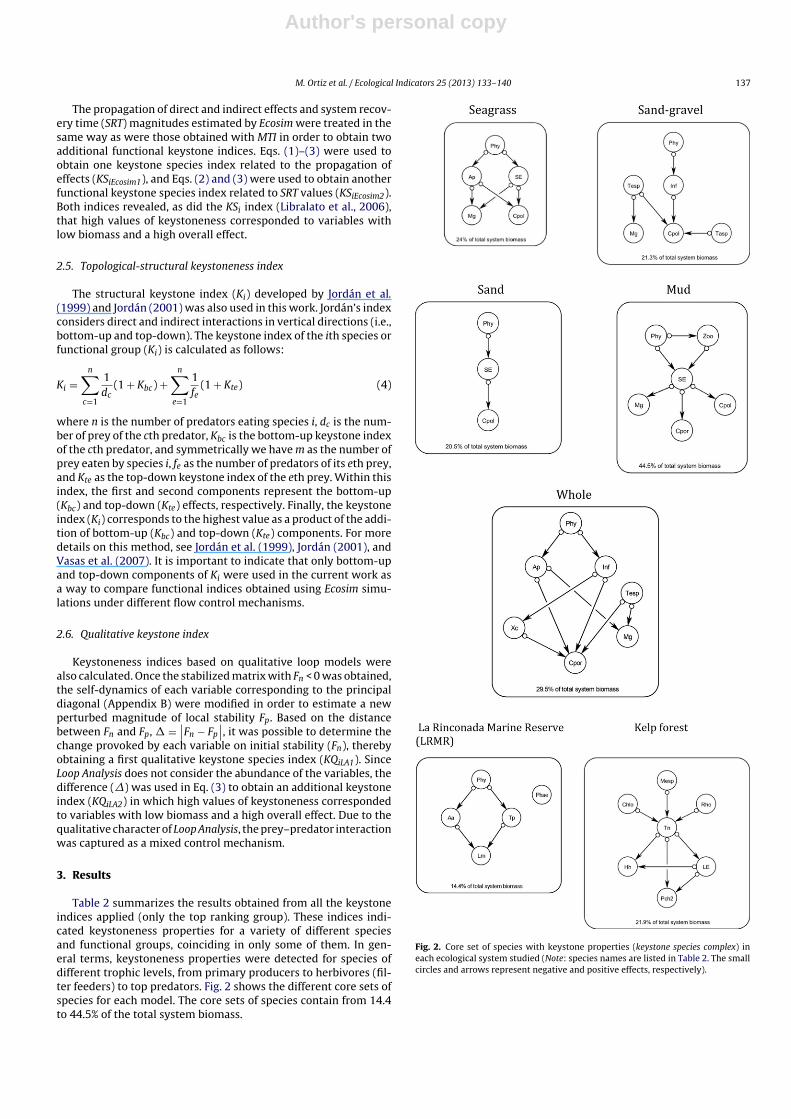
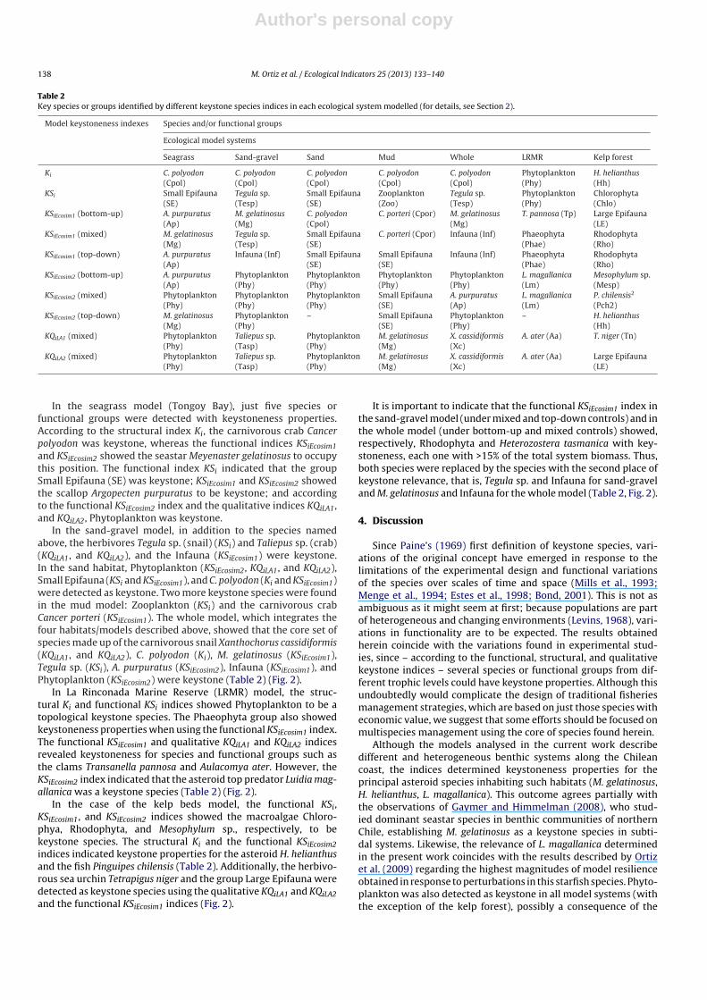
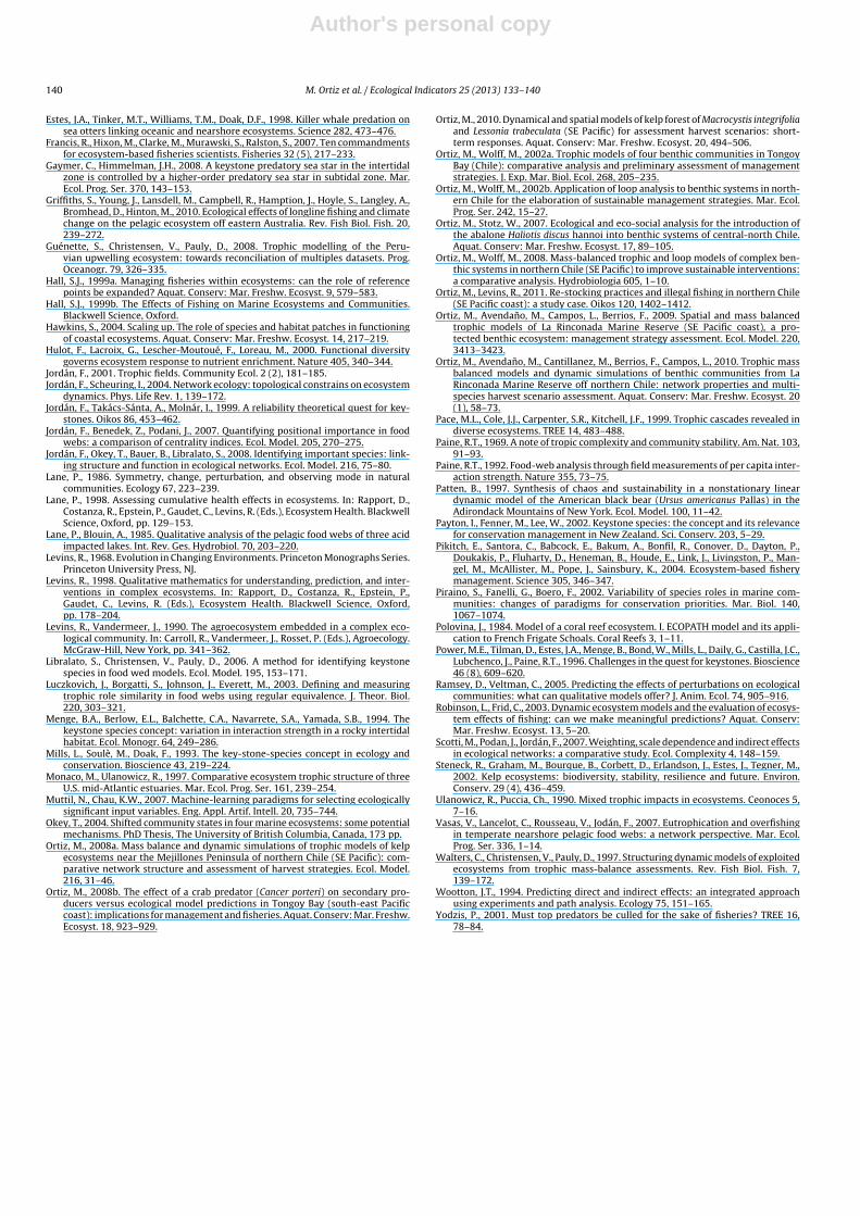
Table 2 summarizes the results obtained from all the keystoneindices applied (only the top ranking group). These indices indi-cated keystoneness properties for a variety of different speciesand functional groups, coinciding in only some of them. In gen-eral terms, keystoneness properties were detected for species ofdifferent trophic levels, from primary producers to herbivores (fil-ter feeders) to top predators. Fig. 2 shows the different core sets ofspecies for each model. The core sets of species contain from 14.4to 44.5% of the total system biomass.

Fig. 2. Core set of species with keystone properties (keystone species complex) ineach ecological system studied (Note: species names are listed in Table 2. The smallcircles and arrows represent negative and positive effects, respectively).

Author's personal copy

138 M. Ortiz et al. / Ecological Indicators 25 (2013) 133–140

Table 2Key species or groups identified by different keystone species indices in each ecological system modelled (for details, see Section 2).

Model keystoneness indexes Species and/or functional groups

Ecological model systems

Seagrass Sand-gravel Sand Mud Whole LRMR Kelp forest

Ki C. polyodon(Cpol)

C. polyodon(Cpol)

C. polyodon(Cpol)

C. polyodon(Cpol)

C. polyodon(Cpol)

Phytoplankton(Phy)

H. helianthus(Hh)

KSi Small Epifauna(SE)

Tegula sp.(Tesp)

Small Epifauna(SE)

Zooplankton(Zoo)

Tegula sp.(Tesp)

Phytoplankton(Phy)

Chlorophyta(Chlo)

KSiEcosim1 (bottom-up) A. purpuratus(Ap)

M. gelatinosus(Mg)

C. polyodon(Cpol)

C. porteri (Cpor) M. gelatinosus(Mg)

T. pannosa (Tp) Large Epifauna(LE)

KSiEcosim1 (mixed) M. gelatinosus(Mg)

Tegula sp.(Tesp)

Small Epifauna(SE)

C. porteri (Cpor) Infauna (Inf) Phaeophyta(Phae)

Rhodophyta(Rho)

KSiEcosim1 (top-down) A. purpuratus(Ap)

Infauna (Inf) Small Epifauna(SE)

Small Epifauna(SE)

Infauna (Inf) Phaeophyta(Phae)

Rhodophyta(Rho)

KSiEcosim2 (bottom-up) A. purpuratus(Ap)

Phytoplankton(Phy)

Phytoplankton(Phy)

Phytoplankton(Phy)

Phytoplankton(Phy)

L. magallanica(Lm)

Mesophylum sp.(Mesp)

KSiEcosim2 (mixed) Phytoplankton(Phy)

Phytoplankton(Phy)

Phytoplankton(Phy)

Small Epifauna(SE)

A. purpuratus(Ap)

L. magallanica(Lm)

P. chilensis2

(Pch2)KSiEcosim2 (top-down) M. gelatinosus

(Mg)Phytoplankton(Phy)

– Small Epifauna(SE)

Phytoplankton(Phy)

– H. helianthus(Hh)

KQiLA1 (mixed) Phytoplankton(Phy)

Taliepus sp.(Tasp)

Phytoplankton(Phy)

M. gelatinosus(Mg)

X. cassidiformis(Xc)

A. ater (Aa) T. niger (Tn)

KQiLA2 (mixed) Phytoplankton(Phy)

Taliepus sp.(Tasp)

Phytoplankton(Phy)

M. gelatinosus(Mg)

X. cassidiformis(Xc)

A. ater (Aa) Large Epifauna(LE)

In the seagrass model (Tongoy Bay), just five species orfunctional groups were detected with keystoneness properties.According to the structural index Ki, the carnivorous crab Cancerpolyodon was keystone, whereas the functional indices KSiEcosim1and KSiEcosim2 showed the seastar Meyenaster gelatinosus to occupythis position. The functional index KSi indicated that the groupSmall Epifauna (SE) was keystone; KSiEcosim1 and KSiEcosim2 showedthe scallop Argopecten purpuratus to be keystone; and accordingto the functional KSiEcosim2 index and the qualitative indices KQiLA1,and KQiLA2, Phytoplankton was keystone.

In the sand-gravel model, in addition to the species namedabove, the herbivores Tegula sp. (snail) (KSi) and Taliepus sp. (crab)(KQiLA1, and KQiLA2), and the Infauna (KSiEcosim1) were keystone.In the sand habitat, Phytoplankton (KSiEcosim2, KQiLA1, and KQiLA2),Small Epifauna (KSi and KSiEcosim1), and C. polyodon (Ki and KSiEcosim1)were detected as keystone. Two more keystone species were foundin the mud model: Zooplankton (KSi) and the carnivorous crabCancer porteri (KSiEcosim1). The whole model, which integrates thefour habitats/models described above, showed that the core set ofspecies made up of the carnivorous snail Xanthochorus cassidiformis(KQiLA1, and KQiLA2), C. polyodon (Ki), M. gelatinosus (KSiEcosim1),Tegula sp. (KSi), A. purpuratus (KSiEcosim2), Infauna (KSiEcosim1), andPhytoplankton (KSiEcosim2) were keystone (Table 2) (Fig. 2).

In La Rinconada Marine Reserve (LRMR) model, the struc-tural Ki and functional KSi indices showed Phytoplankton to be atopological keystone species. The Phaeophyta group also showedkeystoneness properties when using the functional KSiEcosim1 index.The functional KSiEcosim1 and qualitative KQiLA1 and KQiLA2 indicesrevealed keystoneness for species and functional groups such asthe clams Transanella pannosa and Aulacomya ater. However, theKSiEcosim2 index indicated that the asteroid top predator Luidia mag-allanica was a keystone species (Table 2) (Fig. 2).

In the case of the kelp beds model, the functional KSi,KSiEcosim1, and KSiEcosim2 indices showed the macroalgae Chloro-phya, Rhodophyta, and Mesophylum sp., respectively, to bekeystone species. The structural Ki and the functional KSiEcosim2indices indicated keystone properties for the asteroid H. helianthusand the fish Pinguipes chilensis (Table 2). Additionally, the herbivo-rous sea urchin Tetrapigus niger and the group Large Epifauna weredetected as keystone species using the qualitative KQiLA1 and KQiLA2and the functional KSiEcosim1 indices (Fig. 2).

It is important to indicate that the functional KSiEcosim1 index inthe sand-gravel model (under mixed and top-down controls) and inthe whole model (under bottom-up and mixed controls) showed,respectively, Rhodophyta and Heterozostera tasmanica with key-stoneness, each one with >15% of the total system biomass. Thus,both species were replaced by the species with the second place ofkeystone relevance, that is, Tegula sp. and Infauna for sand-graveland M. gelatinosus and Infauna for the whole model (Table 2, Fig. 2).

4. Discussion

Since Paine’s (1969) first definition of keystone species, vari-ations of the original concept have emerged in response to thelimitations of the experimental design and functional variationsof the species over scales of time and space (Mills et al., 1993;Menge et al., 1994; Estes et al., 1998; Bond, 2001). This is not asambiguous as it might seem at first; because populations are partof heterogeneous and changing environments (Levins, 1968), vari-ations in functionality are to be expected. The results obtainedherein coincide with the variations found in experimental stud-ies, since – according to the functional, structural, and qualitativekeystone indices – several species or functional groups from dif-ferent trophic levels could have keystone properties. Although thisundoubtedly would complicate the design of traditional fisheriesmanagement strategies, which are based on just those species witheconomic value, we suggest that some efforts should be focused onmultispecies management using the core of species found herein.

Although the models analysed in the current work describedifferent and heterogeneous benthic systems along the Chileancoast, the indices determined keystoneness properties for theprincipal asteroid species inhabiting such habitats (M. gelatinosus,H. helianthus, L. magallanica). This outcome agrees partially withthe observations of Gaymer and Himmelman (2008), who stud-ied dominant seastar species in benthic communities of northernChile, establishing M. gelatinosus as a keystone species in subti-dal systems. Likewise, the relevance of L. magallanica determinedin the present work coincides with the results described by Ortizet al. (2009) regarding the highest magnitudes of model resilienceobtained in response to perturbations in this starfish species. Phyto-plankton was also detected as keystone in all model systems (withthe exception of the kelp forest), possibly a consequence of the

Author's personal copy

M. Ortiz et al. / Ecological Indicators 25 (2013) 133–140 139

influence of upwelling waters (Daneri et al., 2000; Escribano et al.,2004).

It is relevant to mention that the phytoplankton-zooplanktongroup supports >40% of the overall structure and function in theecological systems of Tongoy Bay (Ortiz and Wolff, 2002a) and LaRinconada Marine Reserve (Antofagasta) (Ortiz et al., 2010). Nev-ertheless, the phytoplankton would be not relevant in kelp forestsbecause the concentration of biomass and contribution of nutrients(through detritus) to the coastal ecosystems would be supported –in this case – by the kelp species (Duggins et al., 1989). In this case,the macroalgae in northern Chile (Antofagasta) would contribute25% of the overall structure and function of the ecosystem (followedby the phyto-zooplankton group with 20%) (Ortiz, 2008a).

The whole model of Tongoy Bay shows an integration of mostspecies and/or groups with keystoneness properties found by habi-tat, and all these species are related ecologically (Fig. 2). A similarsituation appears in La Rinconada Marine Reserve (LRMR) sincetop predators and other species or functional groups from lowand intermediate trophic levels were also determined as keystonespecies. These were Phaeophyta, the scallop A. purpuratus, and theclam T. pannosa. In the case of primary producers, it is possiblethat these indices confused structural and trophic functional prop-erties in the system. On the other hand, the qualitative indicesshowed keystoneness properties for the mussel A. ater. This result isvery interesting since loop model predictions respond with a highdegree of certainty to external perturbations (Briand and McCauley,1978; Lane and Blouin, 1985; Lane, 1986; Hulot et al., 2000; Ortiz,2008b).

The kelp model also showed a core set of species or groupswith keystoneness properties constituted by the fish P. chilensis, theasteroid H. helianthus, Large Epifauna (predators), the sea urchin T.niger (herbivore), and primary producers (the algae Mesophylumsp., Rhodophyta, Chlorophyta). The keystone property of the fishP. chilensis coincides with reports by Ortiz (2008a) that show thatincreased mortality of this fish species by fishing would cause thehighest magnitudes of model resilience in the system. Two qualita-tive keystone indices based on the loop model differed from thoseobtained with the other indices, indicating keystoneness in the her-bivorous sea urchin T. niger (intermediate trophic level) and theLarge Epifauna functional group of predatory crabs (Taliepus denta-tus and Homalaspis plana). The sea urchin T. niger deserves specialattention because, as described in the kelp forests of the SE Pacific,an increased abundance of this herbivore would partially explainthe reduced forests, especially of Macrocystis integrifolia (Stenecket al., 2002).

In general, our results coincide with those reported for ecolog-ical experiments and modelling approaches. That is, species likelyto have keystoneness properties are widely heterogeneous. Jordánet al. (2007, 2008) reported similar findings after comparing severalstructural and functional keystone species indices. The hetero-geneity of possible species or functional groups determined in thecurrent contribution coincide with those described by Power et al.(1996), Piraino et al. (2002), Libralato et al. (2006), and Jordán et al.(2007, 2008), particularly concerning: (1) the difficulty in recog-nizing keystone species in communities and ecosystems with bothexperimental and modelling approaches, and (2) the lack of a gen-eral pattern between trophic levels and keystoneness. Despite thewide heterogeneity of species and/or functional groups with key-stoneness properties, we were still able to observe some interestingtendencies. The core set of species and functional groups consti-tuted by prey/algae and its natural enemies (predators/grazers)reveals a more holistic view of keystoneness, i.e., a keystone speciescomplex, particularly in studies based on quantitative and quali-tative multispecies models such as that constructed herein (seeFig. 2). Okey (2004) described similar results defining keystoneguilds or clusters of species with keystoneness properties based

on a trophic model in Alaska. Thus, we believe that the applicationof this holistic view for keystoneness would facilitate the designand assessment of management strategies in all benthic systemsanalysed. However, we must also recognize that comprehensivemanagement is still quite difficult because: (1) the traditional fish-eries management is based solely on commercial species; and (2)some species within each keystone species complex are intensivelyexploited (such as the bivalves A. purpuratus, A. ater, and T. pannosa;the crabs C. polyodon and Taliepus sp.; the snail X. cassidiformis; andthe fish P. chilensis), reducing their natural densities (this is notthe case of the asteroids). This, without a doubt, imposes an evengreater challenge, since human interventions accompany the net-work of interacting species, co-varying with the variables of thenatural system.

Finally, we know that our results should be contrasted withexperimental studies and other modelling approaches such as thosebased on artificial neural networks (Muttil and Chau, 2007) in orderto increase global understanding of these matters and our capacityfor prediction. Likewise, it is relevant to note that, in spite of theinherent and well-known limitations and shortcomings of the Eco-path, Ecosim and Loop Analysis theoretical frameworks, the modelsconstructed and the simulations executed in the present contribu-tion represent the processes underlying the systems studied onlywhen considering short-term dynamics.

Acknowledgements

This contribution was supported by the Chilean National Foun-dation for Scientific and Technical Development (FONDECYT)(Chile) grant no. 1040293 and CORFO-INNOVA (Chile) grant no.04CR7IPM-01.

Appendix A. Supplementary data

Supplementary data associated with this article can be found, inthe online version, at doi:10.1016/j.ecolind.2012.08.020.

References

Allesina, S., Bodini, A., 2005. Who dominates whom in the ecosystem? Energy flowbottlenecks and cascading extinctions. J. Theor. Biol. 230, 351–358.

Arias, G., González, C., Cabrera, J., Christensen, V., 2011. Predicted impact of the inva-sive lionfish Pterois volitans on the food web of a Caribbean coral reef. Environ.Res. 111 (7), 917–925.

Berlow, E., 1999. Strong effects of weak interactions in ecological communities.Nature 398, 330–334.

Bond, W., 2001. Keystone species – hunting the shark? Science 292, 63–64.Briand, F., McCauley, E., 1978. Cybernetic mechanisms in lake plankton systems:

how to control undesirable algae. Nature 273, 228–230.Brose, U., Berlow, E., Martinez, N., 2005. Scaling up keystone effects from simple to

complex ecological networks. Ecol. Lett. 8, 1317–1325.Christensen, V., Pauly, D., 1992. Ecopath II: a software for balancing steady-state

ecosystem models and calculating network characteristics. Ecol. Model. 61,169–185.

Christensen, V., Walters, C., 2004. Ecopath with Ecosim: methods, capabilities andlimitations. Ecol. Model. 172, 109–139.

Crowder, L., Hazen, E., Avissar, N., Bjorkland, R., Latanich, C., Ogburn, M., 2008. Theimpacts of fisheries on marine ecosystems and the transition to ecosystem-based management. Annu. Rev. Ecol. Syst. 39, 259–278.

Daneri, G., Dellarossa, V., Quinones, R., Jacob, B., Montero, P., Ulloa, O., 2000. Pri-mary production and community respiration in the Humboldt Current Systemoff Chile and associated oceanic areas. Mar. Ecol. Prog. Ser. 197, 41–49.

Darmbacher, J., Guaghan, D., Rochet, M., Rossignol, P., Trenkel, V., 2009. Qualitativemodelling and indicators of exploited ecosystems. Fish and Fish. 10, 305–322.

Duggins, D., Simenstad, C., Estes, J., 1989. Magnification of secondary production bykelp detritus in coastal marine ecosystems. Science 245, 101–115.

Dunne, J., Williams, R., Martinez, N., 2002. Network structure and biodiversity lossin food webs: robustness increases with connectance. Ecol. Lett. 5, 558–567.

Eklöf, A., Ebenman, B., 2006. Species loss and secondary extinctions in simple andcomplex model communities. J. Anim. Ecol. 75, 239–246.

Escribano, R., Rosales, S., Blanco, J.L., 2004. Understanding upwelling circulationoff Antofagasta (northern Chile): a three-dimensional numerical-modelingapproach. Cont. Shelf Res. 24, 37–53.

Author's personal copy

140 M. Ortiz et al. / Ecological Indicators 25 (2013) 133–140

Estes, J.A., Tinker, M.T., Williams, T.M., Doak, D.F., 1998. Killer whale predation onsea otters linking oceanic and nearshore ecosystems. Science 282, 473–476.

Francis, R., Hixon, M., Clarke, M., Murawski, S., Ralston, S., 2007. Ten commandmentsfor ecosystem-based fisheries scientists. Fisheries 32 (5), 217–233.

Gaymer, C., Himmelman, J.H., 2008. A keystone predatory sea star in the intertidalzone is controlled by a higher-order predatory sea star in subtidal zone. Mar.Ecol. Prog. Ser. 370, 143–153.

Griffiths, S., Young, J., Lansdell, M., Campbell, R., Hamption, J., Hoyle, S., Langley, A.,Bromhead, D., Hinton, M., 2010. Ecological effects of longline fishing and climatechange on the pelagic ecosystem off eastern Australia. Rev. Fish Biol. Fish. 20,239–272.

Guénette, S., Christensen, V., Pauly, D., 2008. Trophic modelling of the Peru-vian upwelling ecosystem: towards reconciliation of multiples datasets. Prog.Oceanogr. 79, 326–335.

Hall, S.J., 1999a. Managing fisheries within ecosystems: can the role of referencepoints be expanded? Aquat. Conserv: Mar. Freshw. Ecosyst. 9, 579–583.

Hall, S.J., 1999b. The Effects of Fishing on Marine Ecosystems and Communities.Blackwell Science, Oxford.

Hawkins, S., 2004. Scaling up. The role of species and habitat patches in functioningof coastal ecosystems. Aquat. Conserv: Mar. Freshw. Ecosyst. 14, 217–219.

Hulot, F., Lacroix, G., Lescher-Moutoué, F., Loreau, M., 2000. Functional diversitygoverns ecosystem response to nutrient enrichment. Nature 405, 340–344.

Jordán, F., 2001. Trophic fields. Community Ecol. 2 (2), 181–185.Jordán, F., Scheuring, I., 2004. Network ecology: topological constrains on ecosystem

dynamics. Phys. Life Rev. 1, 139–172.Jordán, F., Takács-Sánta, A., Molnár, I., 1999. A reliability theoretical quest for key-

stones. Oikos 86, 453–462.Jordán, F., Benedek, Z., Podani, J., 2007. Quantifying positional importance in food

webs: a comparison of centrality indices. Ecol. Model. 205, 270–275.Jordán, F., Okey, T., Bauer, B., Libralato, S., 2008. Identifying important species: link-

ing structure and function in ecological networks. Ecol. Model. 216, 75–80.Lane, P., 1986. Symmetry, change, perturbation, and observing mode in natural

communities. Ecology 67, 223–239.Lane, P., 1998. Assessing cumulative health effects in ecosystems. In: Rapport, D.,

Costanza, R., Epstein, P., Gaudet, C., Levins, R. (Eds.), Ecosystem Health. BlackwellScience, Oxford, pp. 129–153.

Lane, P., Blouin, A., 1985. Qualitative analysis of the pelagic food webs of three acidimpacted lakes. Int. Rev. Ges. Hydrobiol. 70, 203–220.

Levins, R., 1968. Evolution in Changing Environments. Princeton Monographs Series.Princeton University Press, NJ.

Levins, R., 1998. Qualitative mathematics for understanding, prediction, and inter-ventions in complex ecosystems. In: Rapport, D., Costanza, R., Epstein, P.,Gaudet, C., Levins, R. (Eds.), Ecosystem Health. Blackwell Science, Oxford,pp. 178–204.

Levins, R., Vandermeer, J., 1990. The agroecosystem embedded in a complex eco-logical community. In: Carroll, R., Vandermeer, J., Rosset, P. (Eds.), Agroecology.McGraw-Hill, New York, pp. 341–362.

Libralato, S., Christensen, V., Pauly, D., 2006. A method for identifying keystonespecies in food wed models. Ecol. Model. 195, 153–171.

Luczkovich, J., Borgatti, S., Johnson, J., Everett, M., 2003. Defining and measuringtrophic role similarity in food webs using regular equivalence. J. Theor. Biol.220, 303–321.

Menge, B.A., Berlow, E.L., Balchette, C.A., Navarrete, S.A., Yamada, S.B., 1994. Thekeystone species concept: variation in interaction strength in a rocky intertidalhabitat. Ecol. Monogr. 64, 249–286.

Mills, L., Soulè, M., Doak, F., 1993. The key-stone-species concept in ecology andconservation. Bioscience 43, 219–224.

Monaco, M., Ulanowicz, R., 1997. Comparative ecosystem trophic structure of threeU.S. mid-Atlantic estuaries. Mar. Ecol. Prog. Ser. 161, 239–254.

Muttil, N., Chau, K.W., 2007. Machine-learning paradigms for selecting ecologicallysignificant input variables. Eng. Appl. Artif. Intell. 20, 735–744.

Okey, T., 2004. Shifted community states in four marine ecosystems: some potentialmechanisms. PhD Thesis, The University of British Columbia, Canada, 173 pp.

Ortiz, M., 2008a. Mass balance and dynamic simulations of trophic models of kelpecosystems near the Mejillones Peninsula of northern Chile (SE Pacific): com-parative network structure and assessment of harvest strategies. Ecol. Model.216, 31–46.

Ortiz, M., 2008b. The effect of a crab predator (Cancer porteri) on secondary pro-ducers versus ecological model predictions in Tongoy Bay (south-east Pacificcoast): implications for management and fisheries. Aquat. Conserv: Mar. Freshw.Ecosyst. 18, 923–929.

Ortiz, M., 2010. Dynamical and spatial models of kelp forest of Macrocystis integrifoliaand Lessonia trabeculata (SE Pacific) for assessment harvest scenarios: short-term responses. Aquat. Conserv: Mar. Freshw. Ecosyst. 20, 494–506.

Ortiz, M., Wolff, M., 2002a. Trophic models of four benthic communities in TongoyBay (Chile): comparative analysis and preliminary assessment of managementstrategies. J. Exp. Mar. Biol. Ecol. 268, 205–235.

Ortiz, M., Wolff, M., 2002b. Application of loop analysis to benthic systems in north-ern Chile for the elaboration of sustainable management strategies. Mar. Ecol.Prog. Ser. 242, 15–27.

Ortiz, M., Stotz, W., 2007. Ecological and eco-social analysis for the introduction ofthe abalone Haliotis discus hannoi into benthic systems of central-north Chile.Aquat. Conserv: Mar. Freshw. Ecosyst. 17, 89–105.

Ortiz, M., Wolff, M., 2008. Mass-balanced trophic and loop models of complex ben-thic systems in northern Chile (SE Pacific) to improve sustainable interventions:a comparative analysis. Hydrobiologia 605, 1–10.

Ortiz, M., Levins, R., 2011. Re-stocking practices and illegal fishing in northern Chile(SE Pacific coast): a study case. Oikos 120, 1402–1412.

Ortiz, M., Avendano, M., Campos, L., Berrios, F., 2009. Spatial and mass balancedtrophic models of La Rinconada Marine Reserve (SE Pacific coast), a pro-tected benthic ecosystem: management strategy assessment. Ecol. Model. 220,3413–3423.

Ortiz, M., Avendano, M., Cantillanez, M., Berrios, F., Campos, L., 2010. Trophic massbalanced models and dynamic simulations of benthic communities from LaRinconada Marine Reserve off northern Chile: network properties and multi-species harvest scenario assessment. Aquat. Conserv: Mar. Freshw. Ecosyst. 20(1), 58–73.

Pace, M.L., Cole, J.J., Carpenter, S.R., Kitchell, J.F., 1999. Trophic cascades revealed indiverse ecosystems. TREE 14, 483–488.

Paine, R.T., 1969. A note of tropic complexity and community stability. Am. Nat. 103,91–93.

Paine, R.T., 1992. Food-web analysis through field measurements of per capita inter-action strength. Nature 355, 73–75.

Patten, B., 1997. Synthesis of chaos and sustainability in a nonstationary lineardynamic model of the American black bear (Ursus americanus Pallas) in theAdirondack Mountains of New York. Ecol. Model. 100, 11–42.

Payton, I., Fenner, M., Lee, W., 2002. Keystone species: the concept and its relevancefor conservation management in New Zealand. Sci. Conserv. 203, 5–29.

Pikitch, E., Santora, C., Babcock, E., Bakum, A., Bonfil, R., Conover, D., Dayton, P.,Doukakis, P., Fluharty, D., Heneman, B., Houde, E., Link, J., Livingston, P., Man-gel, M., McAllister, M., Pope, J., Sainsbury, K., 2004. Ecosystem-based fisherymanagement. Science 305, 346–347.

Piraino, S., Fanelli, G., Boero, F., 2002. Variability of species roles in marine com-munities: changes of paradigms for conservation priorities. Mar. Biol. 140,1067–1074.

Polovina, J., 1984. Model of a coral reef ecosystem. I. ECOPATH model and its appli-cation to French Frigate Schoals. Coral Reefs 3, 1–11.

Power, M.E., Tilman, D., Estes, J.A., Menge, B., Bond, W., Mills, L., Daily, G., Castilla, J.C.,Lubchenco, J., Paine, R.T., 1996. Challenges in the quest for keystones. Bioscience46 (8), 609–620.

Ramsey, D., Veltman, C., 2005. Predicting the effects of perturbations on ecologicalcommunities: what can qualitative models offer? J. Anim. Ecol. 74, 905–916.

Robinson, L., Frid, C., 2003. Dynamic ecosystem models and the evaluation of ecosys-tem effects of fishing: can we make meaningful predictions? Aquat. Conserv:Mar. Freshw. Ecosyst. 13, 5–20.

Scotti, M., Podan, J., Jordán, F., 2007. Weighting, scale dependence and indirect effectsin ecological networks: a comparative study. Ecol. Complexity 4, 148–159.

Steneck, R., Graham, M., Bourque, B., Corbett, D., Erlandson, J., Estes, J., Tegner, M.,2002. Kelp ecosystems: biodiversity, stability, resilience and future. Environ.Conserv. 29 (4), 436–459.

Ulanowicz, R., Puccia, Ch., 1990. Mixed trophic impacts in ecosystems. Ceonoces 5,7–16.

Vasas, V., Lancelot, C., Rousseau, V., Jodán, F., 2007. Eutrophication and overfishingin temperate nearshore pelagic food webs: a network perspective. Mar. Ecol.Prog. Ser. 336, 1–14.

Walters, C., Christensen, V., Pauly, D., 1997. Structuring dynamic models of exploitedecosystems from trophic mass-balance assessments. Rev. Fish Biol. Fish. 7,139–172.

Wootton, J.T., 1994. Predicting direct and indirect effects: an integrated approachusing experiments and path analysis. Ecology 75, 151–165.

Yodzis, P., 2001. Must top predators be culled for the sake of fisheries? TREE 16,78–84.