Identification of the Dynamic Relationship Between Intrapartum Uterine Pressure and Fetal Heart Rate for Normal and Hypoxic Fetuses

IEEE TRANSACTIONS ON BIOMEDICAL ENGINEERING, VOL. 56, NO. 6, JUNE 2009 1587

Identification of the Dynamic Relationship BetweenIntrapartum Uterine Pressure and Fetal Heart Rate

for Normal and Hypoxic FetusesPhilip A. Warrick∗, Member, IEEE, Emily F. Hamilton, Doina Precup,

and Robert E. Kearney, Fellow, IEEE

Abstract—Labor and delivery are routinely monitored electron-ically with sensors that measure and record maternal uterine pres-sure (UP) and fetal heart rate (FHR), a procedure referred to ascardiotocography (CTG). Delay or failure to recognize abnormalpatterns in these recordings can result in a failure to prevent fetalinjury. We address the challenging problem of interpreting intra-partum CTG in a novel way by modeling the dynamic relation-ship between UP (as an input) and FHR (as an output). We use anonparametric approach to estimate the dynamics in terms of animpulse response function (IRF). We apply singular value decom-position to suppress noise, IRF delay, and memory estimation toidentify the temporal extent of the response and surrogate testingto assess model significance. We construct models for a databaseof CTG recordings labeled by outcome, and compare the modelsduring the last 3 h of labor as well as across outcome classes. Theresults demonstrate that the UP–FHR dynamics can be success-fully modeled as an input–output system. Models for pathologicalcases had stronger, more delayed, and more predictable responsesthan those for normal cases. In addition, the models evolved intime, reflecting a clinically plausible evolution of the fetal state dueto the stress of labor.

Index Terms—Biosignal interpretation and diagnostic systems,biosignal modeling, linear and nonlinear dynamical models, signaland image processing.

I. INTRODUCTION

THE LIFELONG disability that can result from oxygendeprivation during childbirth is rare but devastating for

families, clinicians, and the health-care system. The hallmarkindications that significant fetal cerebral hypoxia has occurredduring labor are metabolic acidosis and neurological signs such

Manuscript received June 27, 2008; revised November 27, 2008 and January19, 2009. First published February 20, 2009; current version published June10, 2009. This work was supported by the LMS Medical Systems, Inc., and bythe Natural Sciences and Engineering Research Council of Canada (NSERC).Astericks indicates corresponding author.

∗P. A. Warrick was with LMS Medical Systems, Inc., Montreal, QCH4A 3S5, Canada. He is now with the Department of Biomedical Engi-neering, McGill University, Montreal, QC H3A 2B4, Canada (e-mail: [email protected]).

E. F. Hamilton is with the Department of Obstetrics and Gynecology, McGillUniversity, Montreal, QC H3A 1A1, Canada, and also with LMS MedicalSystems, Inc., Montreal, QC H4A 3S5, Canada (e-mail: [email protected]).

D. Precup is with the School of Computer Science, McGill University,Montreal, QC H3A 2A7, Canada (e-mail: [email protected]).

R. E. Kearney is with the Department of Biomedical Engineering, McGill Uni-versity, Montreal, QC H3A 2B4, Canada (e-mail: [email protected]).

Digital Object Identifier 10.1109/TBME.2009.2014878

as altered levels of consciousness or seizures. Between 1 and 7in 1000 fetuses experience oxygen deprivation during labor thatis severe enough to cause fetal death or brain injury [1]–[3]; therange of this estimate reflects considerable regional variationand some clinical debate on the definition of brain injury. Un-fortunately, noninvasive methods to directly measure the fetalacid–base status and cerebral oxygenation do not exist. Conse-quently, clinicians must rely upon indirect measures of oxygendelivery and neurological function.

A standard approach is cardiotocography (CTG), which mea-sures maternal uterine pressure (UP) and fetal heart rate (FHR);these signals are the cumulative result of many concomitantphysiologies. Visual pattern recognition and inference are thebasis of clinical interpretation. However, these are inconsistentlyapplied [4]. Furthermore, classical patterns have low specificity.Because significant hypoxia is rare, false alarms are common,leading physicians to disregard truly abnormal signals. Indeed,approximately 50% of birth-related brain injuries are deemedpreventable, with incorrect CTG interpretation leading the listof causes [3], [5]–[7]. The social costs of such errors are mas-sive: intrapartum care generates the most frequent malpracticeclaims and the greatest liability costs of all medical special-ties [8]. Thus, there is great motivation to find better methods todiscriminate between healthy and hypoxic conditions.

Clinicians’ interpretation of intrapartum CTG signals relieson the temporary decreases in FHR (FHR decelerations) in re-sponse to uterine contractions. FHR decelerations are mainlydue to two contraction-induced events: 1) umbilical cord com-pression and 2) a decrease in oxygen delivery through an im-paired utero-placental unit. There is general consensus that de-celeration depth, frequency, and timing with respect to con-tractions are indicators of both the insult and the ability of thefetus to withstand it. Fig. 1 shows an example CTG demonstrat-ing this response, where an FHR deceleration follows shortlyafter the onset of each of the four successive uterine contrac-tions. Hypothesis-driven modeling based on this understandingof physiology and clinical interpretation has focused on con-traction and deceleration detection [9]–[14].

In this paper, we propose a new approach that focuses on thedynamic relationship between UP (as an input) and FHR (asan output). Although the FHR is subject to numerous influences(i.e., it is the result of a multiple-input system), UP is the only in-put that is accessible by external monitoring and routinely usedin clinical practice; indeed, clinicians already interpret certainUP–FHR relationships as indications of pathology. We use a

0018-9294/$25.00 © 2009 IEEE

Authorized licensed use limited to: McGill University. Downloaded on June 18, 2009 at 13:09 from IEEE Xplore. Restrictions apply.

1588 IEEE TRANSACTIONS ON BIOMEDICAL ENGINEERING, VOL. 56, NO. 6, JUNE 2009

Fig. 1. CTG stimulus response from four contraction–deceleration pairs over10 min. (a) UP signal with contraction onsets (“C”) indicated. (b) FHR signalwith deceleration onsets (“D”) indicated.

system identification (SI) approach to estimate system dynamicsin terms of an impulse response function (IRF). This model rep-resents very low-frequency (VLF) FHR energy (i.e., <0.03 Hz)linearly related to UP, and is therefore complementary to othercomponents of the FHR normally studied. SI from CTG is achallenge because: 1) measurement disturbances are prevalentand 2) the UP input has narrow bandwidth, is not calibrated, andis subject to unknown measurement delay.

Using a database of CTG recordings labeled by outcome dataavailable after birth, we compared IRFs overtime (during the last3 h of labor) and with respect to their outcome classes (eithernormal or pathological). We found that our method successfullymodeled CTG, and that the models were better for the patho-logical cases; these models consistently explained more of theoutput variance. Model parameters were significantly differentbetween the normal and pathological cases, with the latter hav-ing IRFs with larger gain and longer delay (indicating a strongerand more delayed FHR response to changes in UP). The mod-els also evolved overtime toward stronger and later responses;this progression is consistent with other studies regarding thetiming of acute intrapartum hypoxic injury [15]. These resultssuggest that the model parameters could be useful for the auto-matic classification of the fetal state (as we have done in otherstudies [16], [17] and detail in the discussion).

II. METHODS

A. Data

We used a database consisting of 264 intrapartum CTGrecordings for pregnancies having a birth gestational age greaterthan 36 weeks and having no known genetic malformations [18].We only considered records with at least 3 h of recording.

We labeled each recording by outcome according to its ar-terial umbilical cord base deficit and neonatal indications ofneurological impairment. An elevated base deficit measurementis an important indicator of metabolic acidosis large enough tocause neurological injury [4], [19], [20]. The majority of therecordings were from normal fetuses (221 cases: base deficit<8 mmol/L); the rest were severely pathological (43 cases: basedeficit ≥12 mmol/L, death or evidence of hypoxic ischemic en-cephalopathy). This proportion of pathological cases was muchhigher than their natural incidence [1]–[3].

Fig. 2. Data processing for estimation of UP–FHR dynamics. Preprocessingcleans and segments the UP and FHR into 20-min epochs of input U andoutput f . Nonparametric SI estimates the IRF h, delay d, and memory M . Thesignificance filter validates the resulting models.

Data collection was performed by clinicians using standardclinical fetal monitors to acquire the CTG. The monitors re-ported uniform sampling rates of 4 Hz for FHR [measured inbeats per minute (bpm)] and 1 Hz for UP (measured in millime-ters of mercury), which we up-sampled to 4 Hz by zero-insertionand low-pass filtering. In the majority of cases, the UP or FHRsensors were attached to the maternal abdomen; the FHR wasacquired from an ultrasound probe and the UP was acquiredby tocography. In a few exceptional cases, they were acquiredinternally via an intrauterine (IU) probe and/or a fetal scalpelectrode. UP acquired by an IU probe is considered the gold-standard measurement. Tocography, on the other hand, is notprecisely calibrated; its amplitude depends on the pressure sen-sor contact and abdominal tissue thickness [21]. Additionally,tocography underestimates the duration of contractions [22]. Asa result, the uterine contraction onset in the UP signal is de-layed with respect to that acquired by an IU probe. Jezewskiet al. [23] compared tocography to uterine electromyography, ameasure that is consistent temporally with the IU measurement;they found that in a set of 108 recordings taken within 24 hof labor, the contraction onset, when measured by tocography,occurred later (mean, standard deviation, and maximum valuesof 14, 18, and 80 s, respectively).

B. Overall Processing

We modeled UP–FHR system dynamics by linear SI. Theprocessing steps are shown schematically in Fig. 2. A prepro-cessing step cleaned and segmented the UP and FHR into 20-minepochs of input and output data (U and f ). Next, nonparametricSI methods were used to estimate the IRF (h), the best valuesfor the IRF delay d, and memory M . Finally, the models werevalidated using a model significance filter. Each step is detailednext.

C. Preprocessing

Because it is recorded in a clinical setting, CTG is subject tospecific types of noise. The loss of sensor contact can temporar-ily interrupt the UP or FHR signals, and interference from the(much lower) maternal heart rate can corrupt the FHR. Inter-ruptions appear in the signal as a sharp drop to much loweramplitude followed by a sharp signal restoration. A simplethreshold detector for such segments would be prone to oscil-late for noisy signals near the threshold; to avoid this, we useda Schmitt trigger, which defines separate detection thresholdsfor down-going and up-going transitions. We chose thresholds

Authorized licensed use limited to: McGill University. Downloaded on June 18, 2009 at 13:09 from IEEE Xplore. Restrictions apply.

WARRICK et al.: IDENTIFICATION OF THE DYNAMIC RELATIONSHIP BETWEEN INTRAPARTUM UP AND FHR 1589

of max(µ − αiσ, 0) where µ and σ are the mean and standarddeviation, respectively, over the entire signal; we used α1 = 2and α2 = 1 for the down-going and up-going transitions, re-spectively. Some UP dropout durations were underestimatedby the Schmitt trigger; therefore, we extended dropout seg-ments forward and/or backward in time if their overall standarddeviation remained below a threshold (1 mmHg). We also re-moved segments that had passed the Schmitt trigger but hadnegligible slope over a period of more than 15 s. We merged se-quential dropout segments in close proximity (≤4 samples). Webridged dropouts lasting less than 15 s by linear interpolation;we removed longer dropouts from consideration. We chose allthresholds empirically to obtain a qualitatively acceptable seg-mentation of signal and artifact. More objective segmentationmethods were outside the scope of this study, but are an area ofactive research [24], [25].

Besides UP, FHR is influenced by a number of other physio-logical factors that are unobserved and intrinsic to the fetus (re-flected in FHR baseline and central-nervous-system-regulatedvariability); we did not consider these factors in our input–output model. Also, the UP baseline can fluctuate considerablydepending on the sensor contact. To reduce the impact of thesefactors, we applied a high-pass filter to remove the baseline anda low-pass filter to reduce the variability. We detrended the sig-nals by a high-pass filter selected to pass a long contraction ordeceleration without incurring excessive filter delay. We chosea filter with a cutoff frequency of 1/220 s = 4.5× 10−3 Hz as acompromise between these competing demands. We selected theparameters for low-pass filtering based on two considerations.First, the narrow-band UP energy (i.e., near the contraction rateand �4 Hz) determines the bandwidth of the UP–FHR linearinteraction. However, we also wanted to retain sufficient timeresolution for the delay and memory estimation step (i.e., on theorder of seconds). For these reasons, we decimated the signalsby an antialiasing filter and subsampling to 0.5 Hz .

Model quality generally increases with data length. However,we expected UP–FHR dynamics to be nonstationary since thestate of the fetus tends to degrade with time. To resolve this trade-off, we extracted 20-min epochs with 10 min overlap betweensuccessive epochs; this epoch length is much longer than the typ-ical FHR deceleration response to a contraction (i.e., 1 − 2 min).We extracted as many such epochs as possible starting from thebeginning of a clean (artifact-free) segment; to include any re-maining data at the end of the segment (i.e., <10 min), theoverlap was increased for the last epoch. We estimated modelsfor each epoch.

D. Nonparametric Model

We denote the input UP and output FHR, at time samplen(n = 1, . . . , N), by un and fn , respectively. We modeled theresponse fn to input un as the convolution sum

fn ≈M −1∑i=0

(hi∆t)un−d−i = h ∗ un (1)

where ∆t is the sampling period, and h is the IRF beginningat sample d (called the delay) and of length M (called the

memory). We denote byun the length-M vector of input samples[un−d−M +1 , . . . , un−d−1 , un−d ] used to estimate fn at samplen. For causal (physically realizable) systems, d ≥ 0, but in thepresence of an input measurement delay (as in our case), d maybe negative [26].

Let U be an N × M Toeplitz matrix formed from un . Theleast-squares estimate of h is given by

h = (UT U)−1UT f ≈ Φ−1uuφuf (2)

where, for N � M , UT U and UT f are estimated by the in-put autocorrelation matrix Φuu and the input–output cross-correlation φuf , respectively [26]. Generally, increasing N im-

proves the correlation estimates, and hence, improves h.The residual signal e = f − Uh was used to generate a figure

of merit for the estimated model, in terms of the percent varianceaccounted for (%VAF)

%VAF = 100

(1 − σ2

e

σ2f

)(3)

where σ2e and σ2

f are the variances of the residual and ob-served signals, respectively; lower residual energy correspondsto higher VAFs and better models. VAF calculations excludedthe initial M output samples to avoid filter end effects.

Using VAF to compare normal and pathological models mightbe misleading since difference in FHR variability might con-found the ability of VAF to assess model quality. Therefore, wealso calculated model VAF after low-pass filtering the prepro-cessed FHR. We chose the VLF band below 0.03 Hz (cf., [27])since this frequency band contained practically all (99.97%) ofthe average spectral power of the models; at 0.03 Hz, this powerhad dropped by 35 dB compared to the peak power. We refer tothis VAF measure as VAFVLF .

E. Pseudoinverse for Noise Reduction

The input un was not controlled and was usually a narrow-band signal dominated by the contraction frequency. On theother hand, the FHR was typically rich in frequency content. Inperforming linear SI with such an input, frequencies far from thecontraction frequency will be hard to identify. In other words,the least-squares problem of (2) may be ill-conditioned; spuriousinput–output correlations may result in noisy IRF estimates. Inthis respect, it should be noted that FHR variability at frequen-cies greater than 0.03 Hz will act as noise for the identificationprocedure since there is no power in the UP signal above thisfrequency (i.e., FHR variability is either unrelated or nonlinearlyrelated to UP). These higher frequency components of FHR areknown to contain information that is potentially discriminat-ing [28], [29], which indicates that they may be complementaryto our model. In order to reduce the noise for the linear model,we used singular value decomposition (SVD) and retained onlythe most significant IRF components, as described in [30] andsummarized next.

The noise characteristics of the IRF estimate can be analyzedby examining (UT U)−1 and UT f separately in (2) [31]. First,the Hessian G = UT U is Hermitian and positive definite, so its

Authorized licensed use limited to: McGill University. Downloaded on June 18, 2009 at 13:09 from IEEE Xplore. Restrictions apply.

1590 IEEE TRANSACTIONS ON BIOMEDICAL ENGINEERING, VOL. 56, NO. 6, JUNE 2009

SVD is equivalent to calculating its eigenvectors and eigenvaluesas G = VSVT , where V contains a set of orthonormal vectorsand S is a diagonal matrix. Second, UT f can be rewritten as

UT f = UT Uh + UT e. (4)

Let ρ = VT h and η = VT (UT e) be the projections of the IRFh and the estimated input noise cross-correlation UT e, respec-tively, onto the Hessian eigenvectors V. With these transforma-tions, (2) can be rewritten as

h = VS−1VT (VSρ + Vη)

=M −1∑i=0

(ρi +ηi

si)vi

�=

M −1∑i=0

hi . (5)

Thus, the SVD of G leads to a corresponding decomposition ofh. Equation (5) shows that for small eigenvalues si , the associ-ated noise terms ηi will be amplified and corrupt the model termρi when projected onto the ith eigenvector vi [31]. Limiting thesummation to the most significant eigenvalues should improvethe signal-to-noise ratio of the estimate h. Note that computingthe pseudoinverse of G in this way follows the same decom-position procedure as applying principal components analysis(PCA) or the Karhonen–Loeve transformation (KLT) to the in-put matrix U.

F. Order Estimation

We used the minimum description length (MDL) criterion[32] to choose the number of terms in (5) to retain, given by

MDL(m) =[1 +

mP log(N)N

] N∑i=1

[fi − fi(m)

]2(6)

where m is the number of singular values retained, fi(m) isthe output estimate at the ith time step with m singular valuesretained, and P is a penalty factor, usually set to 1. It is shownin [31] that the summation in (6) can be efficiently calculated asσ2

f −∑m

i=1 si(viT h)2 .

We analyzed the effect of the penalty P on the number ofterms in (6). Our goal was two-fold: first, to maximize IRFquality, as measured by the output VAF; second, to minimizeIRF variability, as measured by the sum of the IRF coefficientabsolute differences

TV =M∑i=0

∣∣hi − hi−1∣∣. (7)

where h−1 and hM are defined to be zero. This measure is calledtotal variation [33] and can be interpreted as the total amplitudeof IRF oscillations.

To resolve the tradeoff between these measures, we comparedthe average VAF and average TV over all epochs for differentvalues of P . From these results and empirical analysis of in-dividual cases, we chose P = 4 for our subsequent modeling.

Fig. 3. Order selection for an example epoch of a pathological case. (a) IRFprincipal components hi (dashed) and cumulative sum

∑hi (solid) for orders

i ≤ 6 are shown. The vertical scales on the IRF plots are identical (zero amplitudeis shown as a dotted horizontal line) and the time units are seconds. With defaultMDL penalty factor P = 1, the IRF included all six components; with selectedP = 4, only the first two components were included. (b) VAF (black circles)and %TV (red triangles) at each order. Compared to the six-component IRF(VAF = 62.9% and TV = 98% of its maximum value), the two-component IRFhad very similar VAF (∼59.1%, indicated by the blue star), but the total variancewas reduced to 22% of its maximum value.

Compared to the results with P = 1, P = 4 reduced averageTV by 70.7% (with a corresponding reduction in TV variance),while only reducing average VAF from 35.9% to 31.5% (a rel-ative reduction of 12.3%). The VAF continued to decrease withhigher values of P , with little improvement in the TV.

Fig. 3(a) shows the effect of changing P on the shape ofthe IRF for an example epoch from a pathological case. Withthe default MDL penalty factor P = 1, the IRF included all sixcomponents; with P = 4, only the first two components wereincluded. Fig. 3(b) shows that the final four components h3,4,5,6contributed little to the output VAF (i.e., they were effectivelynoise); the two-component IRF had very similar VAF (59.1%versus 62.9%), but the TV was substantially reduced (i.e., from98% to 22% of its maximum value).

G. Delay and Memory Estimation

We initially assumed system causality and estimated the IRFswith no delay [i.e., d = 0 in (1)] [34]. However, the input mea-surement delay associated with the UP sensor may result in anegative IRF delay. In contrast, we expect the physiological re-sponse to have a positive delay. The combination of these twodelays can produce an FHR response that occurs before or afterthe measured UP contraction onset (i.e., d could be negativeor positive). We found that better estimates of d led to bettermodel prediction; therefore, we developed an algorithm to esti-mate d for each epoch. Based on [23], we set the lower bound todmin = −480 s. We observed that for some pathological cases,the FHR response occurred as late as 80 s after the UP response,so we set dmax to this value.

Authorized licensed use limited to: McGill University. Downloaded on June 18, 2009 at 13:09 from IEEE Xplore. Restrictions apply.

WARRICK et al.: IDENTIFICATION OF THE DYNAMIC RELATIONSHIP BETWEEN INTRAPARTUM UP AND FHR 1591

The IRF length M should be long enough for the IRF todecay to 0, but as short as possible to improve the conditioningassociated with estimating IRFs, given the short duration ofthe epochs (20 min). Furthermore, UP periodicity introducedartifactual IRF periodicity if M was too long. To handle thisproblem, we performed a search over values of M as well.

The objective of the IRF delay and memory estimation was toidentify the temporal extent of the IRF; this meant searching forIRFs that : 1) started and ended close to zero amplitude, 2) wereas short as possible, and 3) were most predictive of the output.This was not always straightforward because of the IRF pe-riodicity mentioned before. Therefore, we identified candidateintervals that satisfied goal (1), and then chose a best intervalusing the MDL criterion, which implicitly satisfied goals (2)and (3).

Occasionally, when competing candidates had similar MDLvalues, the automatically selected delay and/or memory esti-mates were not consistent with those of neighboring epochs.Therefore, we performed a postprocessing step to choose themost plausible candidate. First, we median-filtered (indepen-dently) the initial selections of delay {di} and recovery {ri} ={di + Mi} over all epochs i as {di} and {ri}. The median fil-tering included up to a total of seven neighboring samples inthe median calculation at each sample and no fewer than foursamples (at the end points). Then, at each epoch i, we chosethe candidate model that was the nearest neighbor to (di , ri ,and MDLi), where MDLi was the MDL of the initial candidateat epoch i; a Euclidean distance metric was used, with eachdimension normalized to units of standard deviation about themean, to give the three dimensions approximately equal weight.In this way, the refined candidates had IRF start and end timevalues that were more consistent with their neighboring epochs.Additionally, their quality remained similar to the initial candi-date.

As a further refinement, we performed a local search forIRFs with minimal starting and ending amplitudes, by vary-ing the d and r found in the previous step by ±10 s. Then,from a final median filtering of d, we removed delays outsidethe 95th percentile of the deviation about the median-filteredvalue at each epoch (considering only epochs with models thathad passed the significance filter, described next). We selectedboth the median filter order and the refinement neighborhoodempirically.

To achieve goal (1), we defined “close” to zero amplitudeas <25% of the maximum IRF amplitude. Therefore, we re-moved models where the first and last IRF lags, h0 and hM −1 ,did not satisfy this criterion (i.e., remove if |hi/hmax | ≥ 0.25,i ∈ {0,M − 1}, where hmax is the IRF maximum amplitude).We considered that delay-memory estimation had not been suc-cessful for these models; furthermore, their VAFs were generallyvery low (the mean, standard deviation, and median values were11.0%, 11.3%, and 6.2%, respectively).

Finally, we removed models having insignificant steady-stategain G < 10−5 (which indicated that UP–FHR dynamics werevirtually absent); the VAFs of these models were also gener-ally very low (the mean, standard deviation, and median val-ues were 8.7%, 11.2%, and 4.6%, respectively). We calculated

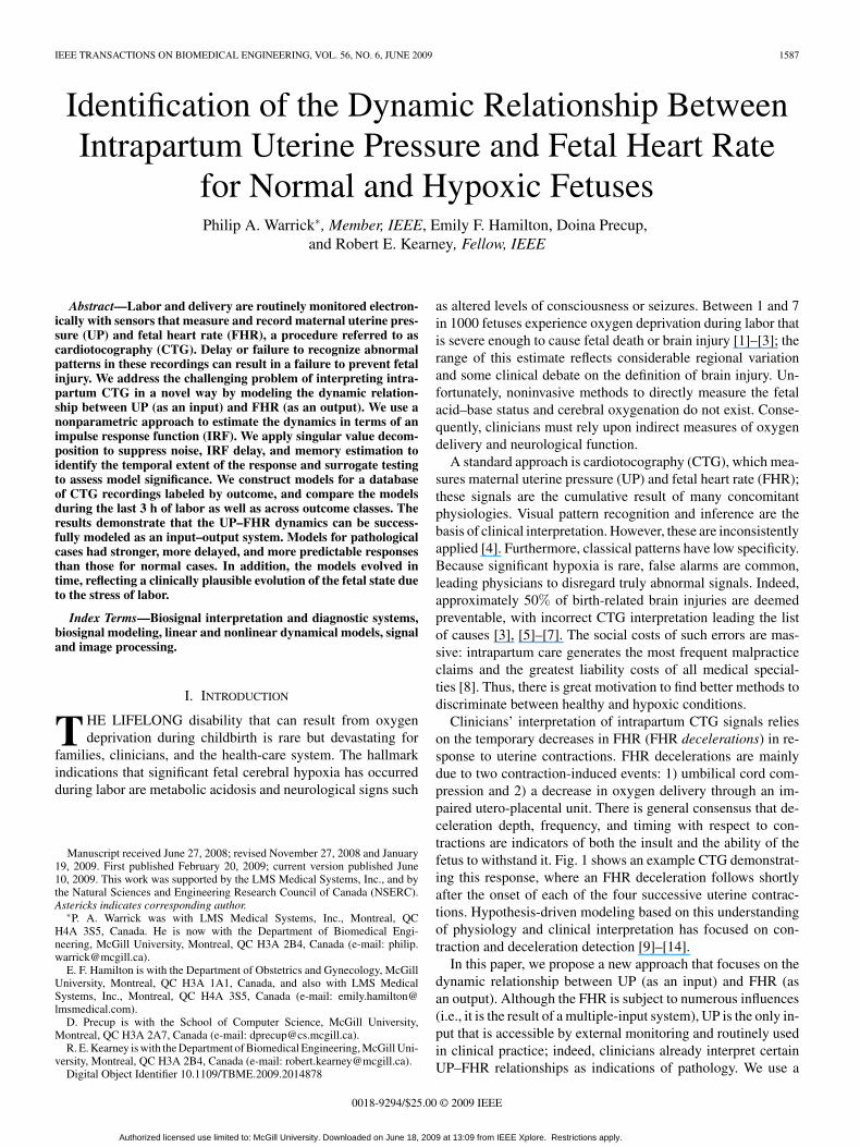
Fig. 4. Acceptance rates of significance validation for (a) normal and (b)pathological cases. For each VAF range, the number of models validated (heightof black bars) out of the total tested (combined height of black and white bars)is shown and the percentage of validated models is indicated.

steady-state gain (henceforth referred to as gain) as the sum ofthe IRF coefficients

G =M −1∑i=0

hi. (8)

H. Determining Model Significance Using Surrogates

Because the model output VAF was often quite low, wewanted to be confident that the IRFs modeled system dynam-ics rather than noise [35]. To do so, we compared IRFs esti-mated from the preprocessed FHR and from multiple FHR sur-rogates; the latter had similar properties to the former, exceptthat their relationship to UP had been destroyed. We generatedthese surrogates using the amplitude adjusted Fourier transform(AAFT) [36], an algorithm that approximately preserves thepower spectrum while maintaining the amplitude probabilitydistribution of the original FHR. However, the process random-izes the phase so any relation to the UP will be removed.

The null hypothesis was that there were no UP–FHR lineardynamics in the epoch. This was rejected when the quality of themodel obtained with the original FHR was superior, statistically,to models computed using surrogate FHR. In particular, themodel was deemed significant if the VAF with the original FHRwas in the 95th percentile of VAFs computed with the originaland surrogate FHRs. This is justified in [36] and [37]. To limitcomputational requirements, we generated Q = 99 surrogates,and chose the parameters of the test to obtain a significancethreshold of 95%.

Fig. 4 shows the model significance validation rates for nor-mal [Fig. 4(a)] and pathological [Fig. 4(b)] cases. The barsfor VAF range 0–100 (at right) shows that overall validationrates were higher for pathological cases (66.8%) than for the

Authorized licensed use limited to: McGill University. Downloaded on June 18, 2009 at 13:09 from IEEE Xplore. Restrictions apply.

1592 IEEE TRANSACTIONS ON BIOMEDICAL ENGINEERING, VOL. 56, NO. 6, JUNE 2009

TABLE IRELATIVE PROPORTION OF EPOCHS ELIMINATED AT EACH PROCESSING

STEP AND FINAL PROPORTION OF VALIDATED EPOCHS FOR NORMAL

AND PATHOLOGICAL CASES

normal cases (54.0%), mainly because pathological cases tendedto have higher VAFs. This is seen in the bars to the left that havemore precise VAF ranges. In particular, pathological cases had asmaller proportion (82/346 = 23.7%) of very low VAF (<10%)compared to the normal cases (917/2322 = 39.4%); these mod-els tended to be rejected for both classes. Acceptance ratesincreased for higher ranges of VAF. For the pathological cases,acceptance was 4.9% for models with VAF < 10%, 63.4% for10%≤VAF < 20%, 88.4% for 20 %≤VAF < 40%, and 100%for models with VAF≥ 40%. These proportions were similarfor the normal cases.

For comparison, to achieve an overall validation acceptancerate equivalent to that obtained with surrogates (55.7%), a hardthreshold of approximately VAF = 13% would have been re-quired. Although our approach also tends to reject low VAFmodels and accept high VAF models, it does so more adap-tively. We note that retaining the FHR variability component(i.e., FHR power ≥40.03 Hz) in the VAF calculation did not af-fect the relative rates of acceptance across classes. The level ofagreement between significance tests that used VAF and thosethat used VAFVLF was 94.9% for normal cases and 95.9% forpathological cases.

III. RESULTS

A. Processing Summary

The proportion of epochs eliminated at each processing step isshown in Table I. A significant portion of the data failed to meetminimum criteria for modeling and were discarded. Preprocess-ing rejected all epochs for 2/221 normal cases and 5/43 patholog-ical cases. Subsequent processing (i.e., removal of models thathad low gain, or that failed delay-memory estimation, or thatdid not pass the significance test using surrogate data) removedall epochs for a further seven pathological and 20 normal cases.We, therefore, retained for analysis 189 normal cases with 1195epochs (out of a possible 3978 epochs, or 30% of the data) and31 pathological cases with 219 epochs (out of 774 epochs, or28% of the data). The pathological data were significantly nois-ier than the normal data: a much larger portion of the formerwas rejected as artifactual during preprocessing (42% versus8% for the normals). On the other hand, of the data that passedthe preprocessing step, a larger proportion of the pathological

Fig. 5. Modeling results for an example epoch of a normal case. (a) Raw inputUP. (b) Preprocessed UP. (c) Raw output FHR. (d) Preprocessed (black) andpredicted (red) output FHR. (e) Residual FHR. (f) Final IRF. Vertical blue barsindicate memory length M = 76s (VAF = 44.7%, d = −16 s, and G = −0.17bpm/mmHg).

cases had models that passed validation (28/(100−42) = 48%)than for the normals (30/(100 − 8) = 33%).

B. IRFs of Typical Epochs

Fig. 5 shows the raw and preprocessed input UP; the raw,preprocessed, and predicted output FHR; the residual e; andestimated IRF for a typical normal epoch. The model pa-rameters were VAF = 44.7%, delay d = −16 s, and gainG = −0.17 bpm/mmHg. This epoch illustrates some of thechallenges to successful modeling of the data. First, the back-ground FHR variability was significant relative to the decelera-tion amplitude. Second, our artifact detection procedure bridgedan FHR dropout at 1100 s, introducing some high-frequency ar-tifact. Despite these factors, the predicted FHR shows that themodel captured the FHR response to UP.

Fig. 6 shows the same signals for a typical pathologicalepoch. In this case, two FHR dropout artifacts were bridged(at 350 and 950 s). Model parameters for the pathological case

Authorized licensed use limited to: McGill University. Downloaded on June 18, 2009 at 13:09 from IEEE Xplore. Restrictions apply.

WARRICK et al.: IDENTIFICATION OF THE DYNAMIC RELATIONSHIP BETWEEN INTRAPARTUM UP AND FHR 1593

Fig. 6. Modeling results for an example epoch of a pathological case. (a) Rawinput UP (b) Preprocessed UP. (c) Raw output FHR. (d) Preprocessed (black)and predicted (red) output FHR. (e) Residual FHR. (f) Final IRF. Verticalblue bars indicate memory length M = 126 s (VAF = 69.6%, d = 34 s, andG = −0.50 bpm/mmHg).

were markedly different from those of the normal case; therewas larger VAF (69.6%), longer delay (d = 34 s), and largergain (G = −0.50 bpm/mmHg) for the pathological case.

The output predictions of Figs. 5(b) and 6(b) (in red) werevery smooth, suggesting that most prediction occurred in thelower frequency band. A frequency analysis of the same epochsconfirmed this. Figs. 7 and 8 show the input UP power spectrumSuu , and the preprocessed and predicted output FHR powerspectra Sf f and Sf f . In both the normal and pathological cases,most of the input and output energies were in the lower frequencyband (i.e., near the UP contraction rate and far below the half-sampling rate of 0.25 Hz). This was the dominant frequencyband of the dynamics and the model accounted for most of theenergy here: the preprocessed and predicted FHR power spectraSf f and Sf f are similar over the main spectral peak (i.e., below∼0.01 Hz). The figure also shows that most of the model power

Fig. 7. Frequency analysis for an example epoch for a normal case. (a) InputUP spectrum Suu (b) Preprocessed (black) and predicted (red) output FHRspectra Sf f and Sf f .

Fig. 8. Frequency analysis for an example epoch for a pathological case. (a)Input UP spectrum Suu (b) Preprocessed (black) and predicted (red) outputFHR spectra Sf f and Sf f .

was contained in the VLF band below 0.03 Hz; at this frequency,the response was attenuated by ∼40 dB with respect to the peakpower. It is also apparent that the higher frequency FHR energy(>0.03 Hz) falls off at later frequencies for the normal comparedto the pathological case, indicating that it contained relativelymore FHR variability.

C. IRF Time Progression of Typical Cases

Fig. 9(a) shows the progression of the IRFs for a normalcase overtime. This case showed marked gain and VAF pro-gression with time: it started at low gain and VAF values (G =−0.136 bpm/mmHg, VAF = 13.7%) and steadily increased toits largest values (G = −0.810 bpm/mmHg, VAF = 58.6%) justbefore delivery. The delay varied between −20 and −4 s.

Fig. 9(b) shows the same time progression for a pathologicalcase. Overall, the pathological case had larger VAF, longer de-lay, and larger gain. The gain was lowest for the initial epochs(G = −0.172 bpm/mmHg, VAF = 37.6%), followed by a largerand relatively stable gain and VAF (G = −0.616 bpm/mmHg,VAF = 54.9%) at epoch −10 until delivery. The delay waslonger and steady for the pathological case (∼16 s). These re-sults are consistent with the clinical expectation that pathologi-cal cases have later and stronger responses.

Authorized licensed use limited to: McGill University. Downloaded on June 18, 2009 at 13:09 from IEEE Xplore. Restrictions apply.

1594 IEEE TRANSACTIONS ON BIOMEDICAL ENGINEERING, VOL. 56, NO. 6, JUNE 2009

Fig. 9. IRF progression over epochs for (a) normal and (b) pathological cases. The perpendicular lines indicate IRF lag t = 0 and the time of delivery (epoch0, marked with triangles). The IRF amplitudes have the same scale with the mesh color ranging from blue (no response) to red (strong response). Overall, thepathological case had longer delay and larger gain. The normal case steadily progressed in time toward its largest gain just before delivery, while the pathologicalcase had lower gain in the first few epochs, but soon increased to a larger gain that remained almost constant until delivery.

Fig. 10. Time progression of model parameters in the last three hours of laborand delivery. The mean and standard error for (a) VAF, (b) VAFVLF (c) gainG, (d) delay d, and (e) memory M are plotted by epoch for normal (blacktriangles) and pathological (red squares) cases. For each parameter, epochswhere hypothesis tests indicated significant differences between classes (p <0.05) are displayed by asterisks (*).

D. IRF Parameters by Class

Fig. 10 shows the time progression, by epoch, of the averagemodel parameters. There were 6 epochs/hour. For the normalcases, the delay was relatively steady overtime. G and VAF,

however, tended to increase overtime, especially in the last hour(i.e., the last six epochs). Overall, the pathological cases hadlonger delay d, larger (negative) gain G, and higher VAF. Forthe pathological cases, the delay increased substantially in thefinal hour; G and VAF increased from the first to second hour,and then dropped in the final hour, likely reflecting the influ-ence of greater sensor disturbance near delivery on the smallerpathological population.

To assess whether the class parameter differences were statis-tically significant, we performed hypothesis tests at each epoch.We compared class distributions with the Kolmogorov–Smirnov(KS) hypothesis test, which uses the maximum difference of theempirical cumulative distribution functions (CDFs) as a teststatistic. More precisely, denoting by FN and FP the CDFsof the normal and pathological populations, respectively, theKS test computes max(|FN (x) − FP (x)|) for all values of themodel parameter x. We deemed a class difference significant ifthe test rejected the null hypothesis at the p < 0.05 level (shownin the figure by blue asterisks). The delay difference was con-sistently significant over the epochs of the final hour. The VAFand gain were significant for most epochs between the end ofhour −3 and hour −2. Memory M did not pass the hypothesistests for significant class differences. We noted that the K-S testwas more conservative than simpler mean-based tests such asthe t-test, which tended to reject the null hypothesis more oftenfor the VAF, delay, and gain parameters.

Using the modified VAFVLF calculation increased the VAF ofthe normal case of Fig. 5 from 44.7% to 54.2% and the patholog-ical case of Fig. 6 from 69.6% to 74.5%. The time progressionof the class average VAFVLF of Fig. 10(b) had a mean trend andvariance that was very similar to the original VAF of Fig. 10(a),except that both the normal and pathological trends were shiftedtowards higher VAF. There was also a slight increase (from 5 to8) in the number of epochs that had statistically significant dif-ferences. These results confirm that the across-class differencesthat we observed in model quality were due mainly to systemdynamics rather than FHR variability.

Authorized licensed use limited to: McGill University. Downloaded on June 18, 2009 at 13:09 from IEEE Xplore. Restrictions apply.

WARRICK et al.: IDENTIFICATION OF THE DYNAMIC RELATIONSHIP BETWEEN INTRAPARTUM UP AND FHR 1595

IV. DISCUSSION

A. Technical Approach

Our SI approach is an entirely automated method that extractsinformation from the two CTG signals in a novel way. The IRFimplicitly captures the strength and timing of the FHR responseto UP, in contrast to a feature detection approach where theserelations must be measured explicitly (e.g., in terms of amplituderatios and time delays) from noisy signals. To our knowledge,this is the first successful attempt to model UP–FHR dynamics.

The particularities of the (uncontrolled) UP input signal re-quired special treatment to regularize the ill-posed identificationproblem. We used SVD decomposition to suppress noise as iscustomary, but instead of using the standard MDL formulation,which tended to generate overly complex IRFs, we used a modi-fied MDL to choose a more appropriate order. The narrow-bandUP introduced periodicity in the estimated IRF; this and theunknown UP sensor measurement delay introduced ambiguityabout the temporal extent of the IRF response. We solved this bydeveloping a method of estimating the IRF delay and memory.

Modeling such data required extensive validation; the finalsurrogate testing provided an objective, adaptive assessment ofmodel quality. When our modeling was successful, our tech-niques generated models that were reliable; they were clean (asevidenced by the reduction in model total variation by the mod-ified MDL criterion for order selection), concise (via the MDLcriterion for delay and memory estimation), and predictive (asevidenced by the VAF). Moreover, these models were consistentwith clinical expectation, as we discuss in the next section.

B. Scientific and Clinical Significance

We have shown that our modeling revealed UP–FHR systemdynamics that correspond well to the clinical understandingof the UP–FHR interaction. Fetuses in distress tend to havestronger and later FHR responses to UP, described in clinicalterms as deeper and later decelerations. Healthy fetuses, on theother hand, tend to respond less overall, and with strong re-sponses only for a short period just prior to delivery. Indeed, ourresults showed significant differences across outcome classesin the IRF parameters corresponding to response strength andtiming (the IRF gain and delay), despite these parameters beingsubject to the measurement problems of UP tocography.

The differences in delay also align with clinical expectation.Sensor-related delays would be expected to affect both outcomeclasses equally; hence, in general, the longer delays in patholog-ical cases were dominated by delays that were physiological innature. This result is also consistent with animal studies, whichhave shown that under conditions of mild hypoxia, relativelyrapid parasympathetic chemo-receptor mechanisms dominatethe fetal response to contractions. However, with increasinghypoxia, slower parasympathetic baroreceptor and direct my-ocardial depression play an increasing role in the decelerationresponse [38], [39]. Consequently, the latency of the fetal re-sponse is expected to increase with hypoxia.

Our finding that models of pathological cases tend to havehigher VAF is also consistent with clinical expectation. In a

healthy fetus, contractions cause little disruption in oxygen de-livery and little need for compensatory FHR changes; a fetus indistress, however, will tend to be less resistant to the insults of la-bor, especially the highly compressive contraction events. Theircompensatory mechanisms may be quite compromised, causingthem to follow rather than resist the onslaught of the stimulus.As a result, their response is a more predictable phenomenonthat can be modeled more precisely.

Clinical UP and FHR are very noisy signals prone to frequentsensor disturbance; to our knowledge, CTG signals collectedunder these conditions have never been subject to the analysisof an approach such as ours. The pathological cases were espe-cially prone to artifact, suggesting that these cases were morelikely subject to sensor disturbance and clinical intervention.Despite these conditions, our modeling successfully generatedvalid models for around a third of the data (including artifac-tual data). Furthermore, the proportion of artifact-free epochsresulting in models was higher for pathological cases (one-half)compared to the normal cases (one-third). We think that thissuccess rate is very acceptable: normal cases often exhibit sig-nificant FHR response to UP only very late in labor (i.e., thereis often a weak or nonexistent UP/FHR model). Consequently,it is to be expected that no model would be found for manyepochs where there is no response; these should not raise analarm because they are consistent with the behavior of healthyfetuses. Pathological cases tend to have an FHR response to UPthat is more significant and occurring earlier in labor, but theymay also have no response due to severe loss of compensatorymechanisms (which may be indicative of chronic rather thanacute injury). Therefore, even if the data were artifact-free, wewould not expect to generate models for every epoch.

C. Classification

Our results suggest that the model parameters could be usedsuccessfully to automatically classify the fetal state. Indeed, inother studies, we have successfully used our model, in con-junction with measures of FHR variability and baseline, forclassification purposes. Using the SI model alone for epochsnear delivery, we reported a false positive rate of 10% (i.e., aspecificity of 90%) with a sensitivity of ∼75% (i.e., a false neg-ative rate of 25%) [16]. This classification considered epochsin isolation; for a more robust classifier, we also considered thehistory of epoch classifications [17]. With this approach, weobserved a mean area under the receiver–operator characteris-tic (ROC) of 0.801. This ROC was generated by varying thenumber of single-epoch pathological classifications required togenerate an overall pathological classification (i.e., varying fromone to six epochs). For comparison, we also generated similarclassifiers that used measures of FHR baseline and variabilityas features. These features were generated by linear fitting forthe baseline and an autoregressive (AR) model for the vari-ability. A study of individual pathological cases indicated thatsome fetuses were classified by one or the other, but not both ofthe classifiers. Of the 31 pathological cases tested (selected tohave at least three SI models), five were correctly classified bythe SI model classifier alone, four were correctly classified by

Authorized licensed use limited to: McGill University. Downloaded on June 18, 2009 at 13:09 from IEEE Xplore. Restrictions apply.

1596 IEEE TRANSACTIONS ON BIOMEDICAL ENGINEERING, VOL. 56, NO. 6, JUNE 2009

the baseline-variability classifier alone, 18 were correctly classi-fied by both, and four were missed by both. These results clearlydemonstrate the potential clinical significance of our models aswell as the complementarity of the SI model, and measures ofFHR variability and baseline.

D. Future Work

We expect that better UP measurement techniques, such asuterine electromyography [40], would improve discriminationof the two classes further. Indeed, further insights could beobtained by applying our approach to data collected with animproved acquisition protocol.

The generally low VAFs can be attributed to that fact thatUP is not the only influence on FHR. Background intrinsicFHR variability unrelated to UP can be of significant ampli-tude [41]. Also, our linear model assumes stationarity withinepochs (which can be violated) and does not account for non-linear interactions such as: 1) the higher frequency harmonicspresent in some very sharp decelerations and 2) variability thatis coincident with decelerations [42]. We are also aware that cer-tain severely injured fetuses may display FHR with abnormalvariability or levels of baseline [28], [29]. We view our VLF SImodel as complementary to measures of FHR variability andbaseline for assessment of the fetal state.

We also hope to classify intermediate cases, which may de-velop hypoxia quite late in delivery. A survey of clinical FHRstudies [4] concluded that fetal acidemia usually develops over1 h. Given fetal-state evolution over this time frame, there isgreat potential for the combination of better data collection andmodel-based analysis to improve current clinical practice byidentifying fetuses at risk before they become injured.

REFERENCES

[1] ACOG, Neonatal Encephalopathy and Cerebral Palsy: Defining the Patho-genesis and Pathophysiology. Washington, DC: ACOG Task force onNeonatal Encephalopathy and Cerebral Palsy, Jan. 2003.

[2] N. Badawi, J. Kurinczuk, J. Keogh, L. Alessandri, F. O’Sullivan, P. Burton,P. Pemberton, and F. Stanley, “Antepartum risk factors for newborn en-cephalopathy: The Western Australian case-control study,” BMJ, vol. 317,pp. 1549–1553, 1998.

[3] E. Draper, J. Kurinczuk, C. Lamming, M. Clarke, D. James, and D. Field,“A confidential enquiry into cases of neonatal encephalopathy,” Arch.Dis. Child Fetal Neonatal Ed., vol. 87, pp. F176–F180, 2002.

[4] J. T. Parer, T. King, S. Flanders, M. Fox, and S. J. Kilpatrick, “Fetalacidemia and electronic fetal heart rate patterns: Is there evidence of anassociation?,” J. Matern.-Fetal Neonatal Med., vol. 19, no. 5, pp. 289–294, May 2006.

[5] S. Ransom, D. Studdert, M. Dombrowski, J. Mello, and T. Brennan, “Re-duced medicolegal risk by compliance with obstetric clinical pathways: Acase-control study,” Obstet. Gynecol., vol. 101, no. 4, pp. 751–755, 2003.

[6] C. Saphier, E. Thomas, D. Studdert, T. Brennan, and D. Acker, “Apply-ing no-fault compensation to obstetric malpractice claims,” Prim. CareUpdate Ob./Gyns., vol. 5, pp. 208–209, 1998.

[7] B. Stalnaker, J. Maher, G. Kleinman, J. Macksey, L. Fishman, andJ. Bernard, “Characteristics of successful claims for payment by theFlorida Neurologic Injury Compensation Association Fund,” Amer. J.Obstet. Gynecol., vol. 177, pp. 268–271, 1997.

[8] G. Berry and P. Martin, “Perinatal risks. Risk management foundation har-vard medical institutions forum,” Harvard Univ., Cambridge, MA,Tech.Rep., Mar. 2001.

[9] K. Maeda, M. Utsu, A. Makio, M. Serizawa, Y. Noguchi, T. Hamada,K. Mariko, and F. Matsumoto, “Neural network computer analysis of fetalheart rate,” J. Matern.-Fetal Invest., vol. 8, no. 4, pp. 163–171, Dec. 1998.

[10] J. Skinner, J. Garibaldi, J. Curnow, and E. Ifeachor, “Intelligent fetal heartrate analysis,” in Proc. 1st Int. Conf., Adv. Med. Signal Inf. Process., 2000,pp. 14–21, (Inst. Electr. Eng. Conf. Publ. No. 476).

[11] F. Lunghi, G. Magenes, L. Pedrinazzi, and M. Signorini, “Detection offetal distress though a support vector machine based on fetal heart rateparameters,” in Proc. Comput. Cardiol., 2005, pp. 247–250.

[12] P. Warrick, E. Hamilton, and M. Macieszczak, “Neural network baseddetection of fetal heart rate patterns,” in Proc. 2005 IEEE Int. Joint Conf.Neural Netw., vol. 4, pp. 2400–2405.

[13] H. Cao, D. Lake, J. E. Ferguson, II, C. Chisholm, M. Griffin, andJ. Moorman, “Toward quantitative fetal heart rate monitoring,” IEEETrans. Biomed. Eng., vol. 53, no. 1, pp. 111–118, Jan. 2006.

[14] G. Georgoulas, D. Stylios, and P. Groumpos, “Predicting the risk ofmetabolic acidosis for newborns based on fetal heart rate signal clas-sification using support vector machines,” IEEE Trans. Biomed. Eng.,vol. 53, no. 5, pp. 875–884, May 2006.

[15] F. Cowan, M. Rutherford, F. Groenendaal, P. Eken, E. Mercuri,G. M. Bydder, L. C. Meiners, L. M. Dubowitz, and L. S. de Vries, “Originand timing of brain lesions in term infants with neonatal encephalopathy,”Lancet, vol. 361, no. 9359, pp. 736–742, Mar. 2003.

[16] P. A. Warrick, E. F. Hamilton, R. E. Kearney, and D. Precup, “Classi-fication of normal and hypoxic fetuses using system identification fromintra-partum cardiotocography,” presented at the ICML 2008 WorkshopMach. Learning Health Care Appl. Helsinki, Finland.

[17] P. A. Warrick, E. F. Hamilton, D. Precup, and R. E. Kearney, “Classificationof normal and hypoxic fetuses from systems modelling of intra-partumcardiotocography,” IEEE Trans. Biomed. Eng., 2009, to be published.

[18] E. Hamilton, A. Dyachenko, C. Elliott, P. Warrick, and A. Ciampi,“Progression of intrapartum EFM patterns in births with symptomaticmetabolic acidosis,” Amer. J. Obstet. Gynecol., vol. 197, no. 6, p. s182,2007.

[19] J. Low, R. Victory, and E. Derrick, “Predictive value of electronic fe-tal monitoring for intrapartum fetal asphyxia with metabolic acidosis,”Obstet. Gynecol., vol. 93, pp. 285–291, 1999.

[20] A. MacLennan, “A template for defining a causal relation between acuteintrapartum events and cerebral palsy: International consensus statement,”BMJ, vol. 319, no. 7216, pp. 1054–1059, 1999.

[21] T. Vanner and J. Gardosi, “Intrapartum assessment of uterine activity,”Bailliere’s Clin. Obstet. Gynaecol., vol. 10, no. 2, pp. 243–257, Jun.1996.

[22] A. M. Miles, M. Monga, and K. S. Richeson, “Correlation of external andinternal monitoring of uterine activity in a cohort of term patients,” Amer.J. Perinatol., vol. 18, no. 3, pp. 137–140, 2001.

[23] J. Jezewski, K. Horoba, A. Matonia, and J. Wrobel, “Quantitative analysisof contraction patterns in electrical activity signal of pregnant uterus asan alternative to mechanical approach,” Physiol. Meas., vol. 26, no. 5,pp. 753–767, 2005.

[24] M. Davy and S. Godsill, “Detection of abrupt spectral changes usingsupport vector machines an application to audio signal segmentation,”in Proc. IEEE Int. Conf. Acoust., Speech, Signal Process., 2002, vol. 2,pp. 1313–1316.

[25] B. Aysin, L. Chaparro, I. Grave, and V. Shusterman, “Orthonormal-basispartitioning and time-frequency representation of cardiac rhythm dynam-ics,” IEEE Trans. Biomed. Eng., vol. 52, no. 5, pp. 878–889, May 2005.

[26] I. W. Hunter and R. E. Kearney, “Two-sided linear filter identification,”Med. Biol. Eng. Comput., vol. 21, pp. 203–209, 1983.

[27] S. Cerutti, S. Civardi, A. Bianchi, M. Signorini, E. Ferrazzi, and G. Pardi,“Spectral analysis of antepartum heart rate variability,” Clin. Phys. Phys-iol. Meas., vol. 10, pp. 27–31, 1989.

[28] International Federation of Gynecology Obstetrics (FIGO), “Guidelinesfor the use of fetal monitoring,” Int. J. Gynaecol. Obstet., vol. 25, pp. 159–67, 1987.

[29] National Institute of Child Health Human Development (NICHD),“Electronic fetal heart rate monitoring: Research guidelines for interpre-tation. National institute of child health and human development researchplanning workshop,” Amer. J. Obstet. Gynecol., vol. 177, no. 6, pp. 1385–1390, 1997.

[30] P. A. Warrick, R. E. Kearney, D. Precup, and E. F. Hamilton, “System-identification noise suppression for intra-partum cardiotocography to dis-criminate normal and hypoxic fetuses,” in Proc. Comput. Cardiol., 2006,vol. 33, pp. 937–940.

[31] D. T. Westwick and R. E. Kearney, Identification of Nonlinear Physiolog-ical Systems. Hoboken, NJ: Wiley Interscience, 2003.

[32] J. Rissanen, “Modeling by shortest data description,” Automatica, vol. 14,pp. 465–471, 1978.

Authorized licensed use limited to: McGill University. Downloaded on June 18, 2009 at 13:09 from IEEE Xplore. Restrictions apply.

WARRICK et al.: IDENTIFICATION OF THE DYNAMIC RELATIONSHIP BETWEEN INTRAPARTUM UP AND FHR 1597

[33] S. Mallat, A Wavelet Tour of Signal Processing. San Diego, CA: Aca-demic, 1999.

[34] P. A. Warrick, E. F. Hamilton, D. Precup, and R. E. Kearney, “Detectingthe temporal extent of the impulse response function from intra-partumcardiotocography for normal and hypoxic fetuses,” in Proc. 2008 IEEEEng. Med. Biol. 30th Annu. Conf., 2009, pp. 2797–2800.

[35] P. A. Warrick, R. E. Kearney, D. Precup, and E. F. Hamilton, “Time pro-gression of a parametric impulse response function estimate from intra-partum cardiotocography for normal and hypoxic fetuses,” in Proc. Com-put. Cardiol., 2007, pp. 693–696.

[36] J. Theiler, S. Eubank, A. Longtin, B. Galdrikian, and J. D. Farmer, “Testingfor nonlinearity in time series: The method of surrogate data,” Phys. D,Nonlinear Phenom., vol. 58, no. 1–4, pp. 77–94, Sep. 1992.

[37] T. Schreiber and A. Schmitz, “Surrogate time series,” Phys. D, NonlinearPhenom., vol. 142, no. 3–4, pp. 346–382, Aug. 2000.

[38] C. B. Martin, J. de Haan, B. van der Wildt, H. W. Jongsma, A. Dieleman,and T. H. M. Arts, “Mechanisms of late decelerations in the fetal heartrate: A study with autonomic blocking agents in fetal lambs,” Eur. J.Obstet. Gynecol. Reprod. Biol., vol. 9, no. 6, pp. 361–373, Dec. 1979.

[39] L. Bennet, J. A. Westgate, Y.-C. J. Liu, G. Wassink, and A. J. Gunn, “Fetalacidosis and hypotension during repeated umbilical cord occlusions areassociated with enhanced chemoreflex responses in near-term fetal sheep,”J. Appl. Physiol., vol. 99, no. 4, pp. 1477–1482, 2005.

[40] M. Skowronski, J. Harris, D. Marossero, R. Edwards, and T. Euliano, “Pre-diction of intrauterine pressure from electrohysterography using optimallinear filtering,” IEEE Trans. Biomed. Eng., vol. 53, no. 10, pp. 1983–1989, Oct. 2006.

[41] J. Westgate, B. Wibbens, L. Bennet, G. Wassink, J. Parer, and A. Gunn,“The intrapartum deceleration in center stage: A physiologic approach tothe interpretation of fetal heart rate changes in labor,” Amer. J. Obstet.Gynecol., vol. 197, no. 3, pp. 236.e1–236.e11, 2007.

[42] M. Romano, P. Bifulco, M. Cesarelli, M. Sansone, and M. Bracale, “Foetalheart rate power spectrum response to uterine contraction,” Med. Biol.Eng. Comput., vol. 44, no. 3, pp. 188–201, Mar. 2006.

Philip A. Warrick (S’07–M’07) received theB.A.Sc. degree in electrical engineering from theUniversity of Waterloo, Waterloo, ON, Canada, in1987, and the M.Eng. degree in electrical engineer-ing from McGill University, Montreal, QC, Canada.,where he is currently working toward the Ph.D.degree.

He was engaged in the industry in biomedicalapplications. From 2000 to 2004), he was a SeniorMedical Research Engineer at LMS Medical Sys-tems, Inc. His current research interests include sys-

tems modeling, statistical signal processing, machine learning, and decisionsupport systems. His research aims to develop better methods of acquiring andinterpreting biomedical signals to facilitate improved clinical decision making.

Emily F. Hamilton received the B.Sc. degree fromBishop’s University, QC, Canada, the MDCM de-gree from McGill University, Montreal, QC, and theFRCSC degree from the Royal College of Physiciansand Surgeons of Canada.

She is currently is the Chief Medical Officer atLMS Medical Systems, Inc., Montreal, QC, Canada.She is also an Adjunct Professor of obstetrics andgynecology at McGill University, Montreal, whereshe was also the Director of the Residency EducationProgram in Obstetrics and Gynecology, and the Di-

rector of Perinatology.She is an experienced Obstetrician. She is also a member of various

Canadian National Task Forces defining Clinical Practice Guidelines for fetalsurveillance.

Doina Precup received the B.Eng. degree from theTechnical University of Cluj-Napoca, Cluj-Napoca,Romania, in 1994, and the M.Sc. and Ph.D. degreesfrom the University of Massachusetts, Amherst, in1997 and 2000, respectively, all in computer sci-ence. Her graduate studies were funded in part by aFulbright fellowship.

She is currently an Associate Professor in theSchool of Computer Science, McGill University,Montreal, QC, Canada. Her current research inter-ests include artificial intelligence, machine learning,

and the application of these methods to real-world time series data.

Robert E. Kearney (M’96–SM’92–F’01) receivedthe B.Eng., M.Eng., and Ph.D. degrees from McGillUniversity, Montreal, QC, Canada.

He is currently a Professor in the Depart-ment of Biomedical Engineering, McGill University,Montreal, QC, Canada, where he has been engagedin maintaining an active research program that fo-cuses on using quantitative engineering techniques toaddress important biomedical problems. His currentresearch interests include the development of algo-rithms and tools for biomedical system identification,

the application of system identification to understand the role played by periph-eral mechanisms in the control of posture and movement, and the developmentof bioinformatics tools and techniques for proteomics.

Dr. Kearney is a Fellow of the Engineering Institute of Canada and the Amer-ican Institute of Medical and Biological Engineering. He was the recipient ofthe IEEE Millennium Medal.

Authorized licensed use limited to: McGill University. Downloaded on June 18, 2009 at 13:09 from IEEE Xplore. Restrictions apply.