Identification of material parameters for springback ...rdo.psu.ac.th/sjstweb/journal/38-5/38-5-4.pdf · In sheet metal forming process, springback is a critical problem for die makers,

Original Article

Identification of material parameters for springback predictionusing cyclic tension–compression test

Thaweesak Phongsai1, Weerapong Julsri1, Bunyong Chongthairungruang1, Surasak Suranuntchai1,Suwat Jirathearanat3, and Vitoon Uthaisangsuk2*

1 Department of Tool and Materials Engineering,

2 Department of Mechanical EngineeringFaculty of Engineering, King Mongkut’s University of Technology Thonburi, Thung Khru, Bangkok, 10140 Thailand.

3 National Metal and Materials Technology Centre, National Science and Technology Development AgencyKhlong Luang, Pathum Thani, 12120 Thailand.

Received: 6 July 2015; Accepted: 20 January 2016

Abstract

In sheet metal forming process, springback is a critical problem for die makers, particularly in case of advanced highstrength steels. Therefore, FE simulations were often used to calculate materials deformation behavior and the springbackoccurrence of formed sheet metals. Recently, the Yoshida–Uemori model, a kinematic hardening model, has shown greatcapability for describing the elastic recovery of a material. Nevertheless, determination of model parameters is sophisticatedfor industrial applications. In this work, an AHS steel grade JIS JSC780Y was investigated, in which tension–compressiontests were carried out and the procedure of parameter identification was analyzed. Different fitting methods were examinedand verified by evaluation of cyclic stress–strain responses obtained from simulations of 1–element model and experiments.The most appropriate parameter set was determined. Finally, hat shape forming test was performed and springback obtainedby calculation and experiment was compared. It was found that the introduced procedure could be acceptably applied.

Keywords: high strength steel, springback, Yoshida-Uemori model, material parameters

Songklanakarin J. Sci. Technol.38 (5), 485-493, Sep. - Oct. 2016

1. Introduction

At present, production of automotive componentshave become very high competitive. Thus, part manufac-turers require shorter time for developing dies. Besides, moreaccurate methods are needed in order to improve the qualityof produced parts. For current automotive parts, advancedhigh strength (AHS) steel grades have been continuouslyintroduced and employed so that both lightweight and higherstrength characteristics are fulfilled. However, one greatchallenge of AHS steels in the forming process is the

springback effect. It significantly affects the final shape ofparts and can raise critical problems by the part assembly.To precisely describe this behavior of such steels is sophisti-cated. Die makers as well as researchers have paid muchattention to prediction and compensation of the springback(Carden et al., 2002; Gan et al., 2004). In the industries, finiteelement (FE) simulation has been widely employed in supportof springback description. Accuracies of the FE simulationresults depend not only on forming process parameters liketools and binder geometries, contact conditions, but also onthe choice of the material’s constitutive model. The materialmodel plays an important role for calculating deformationbehavior of formed sheet metal, which greatly influencesarising elastic recovery, residual stresses and correspondingspringback. Different types of material constitutive laws such

* Corresponding author.Email address: [email protected]

http://www.sjst.psu.ac.th

T. Phongsai et al. / Songklanakarin J. Sci. Technol. 38 (5), 485-493, 2016486

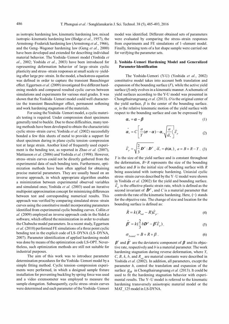
as isotropic hardening law, kinematic hardening law, mixedisotropic–kinematic hardening law (Hodge et al., 1957), theArmstrong–Frederick hardening law (Armstrong et al., 1966),and the Geng–Wagoner hardening law (Geng et al., 2000)have been developed and extended for describing individualmaterial behavior. The Yoshida–Uemori model (Yoshida etal., 2002; Yoshida et al., 2003) have been introduced forrepresenting deformation behavior of large–strain cyclicplasticity and stress–strain responses at small scale re–yield-ing after large pre–strain. In the model, a backstress equationwas defined in order to capture the transient Bauschingereffect. Eggertsen et al. (2009) investigated five different hard-ening models and compared resulted cyclic curves betweensimulations and experiments for various steel grades. It wasshown that the Yoshida–Uemori model could well character-ize the transient Bauschinger effect, permanent softeningand work hardening stagnation of the materials.

For using the Yoshida–Uemori model, a cyclic materi-als testing is required. Under compression sheet specimensgenerally tend to buckle. Due to these difficulties, many test-ing methods have been developed to obtain the characteristiccyclic stress–strain curve; Yoshida et al. (2002) successfullybonded a few thin sheets of metal to provide a support forsheet specimen during in plane cyclic tension–compressiontest at large strain. Another kind of frequently used experi-ment is the bending test, as reported in Zhao et al. (2007),Mattiasson et al. (2006) and Yoshida et al. (1998). However,stress–strain curves could not be directly gathered from theexperimental data of such bending tests. Furthermore, opti-mization methods have been often applied for obtainingprecise material parameters. They are usually based on aninverse approach, in which appropriate algorithm enablesa minimization between experimental observed variablesand simulated ones; Yoshida et al. (2003) used an iterativemultipoint approximation concept for minimizing differencesbetween test and corresponding numerical results. Thisapproach was verified by comparing simulated stress–straincurves using the constitutive model incorporating parametersidentified from experimental cyclic bending curves. Collin etal. (2009) employed an inverse approach code in the SidoLosoftware, which offered the minimization in order to evaluatethe Chaboche model parameters. In a recent study, Eggertsenet al. (2010) performed FE simulations of a three point cyclicbending test in the explicit code of LS–DYNA (LS–DYNA,2007). Parameter identification of applied hardening modelwas done by means of the optimization code LS-OPT. Never-theless, such optimization methods are still not suitable forindustrial purposes.

The aim of this work was to introduce parameterdetermination procedures for the Yoshida–Uemori model by asimple fitting method. Cyclic tension–compression experi-ments were performed, in which a designed sample fixtureinstallation for preventing buckling by spring force was usedand a video extensometer was employed to measure thesample elongation. Subsequently, cyclic stress–strain curveswere determined and each parameter of the Yoshida–Uemori

model was identified. Different obtained sets of parameterswere evaluated by comparing the stress–strain responsesfrom experiments and FE simulations of 1–element model.Finally, forming tests of a hat shape sample were carried outfor verifying the parameter sets.

2. Yoshida–Uemori Hardening Model and GeneralizedParameter Identification

The Yoshida-Uemori (Y-U) (Yoshida et al., 2002)constitutive model takes into account both translation andexpansion of the bounding surface (F), while the active yieldsurface (f) only evolves in a kinematic manner. A schematic ofyield surfaces according to the Y-U model was presented inChongthairungruang et al. (2013). O is the original center ofthe yield surface, is the center of the bounding surface. is the relative kinematic motion of the yield surface withrespect to the bounding surface and can be expressed by

* (1)

*

( ) p

a aC

Y

* *

(2)

2:

3p p

p D D , * *( ) , a B R Y . (3)

Y is the size of the yield surface and is constant throughoutthe deformation, B+R represents the size of the boundingsurface and B is the initial size of bounding surface with Rbeing associated with isotropic hardening. Uniaxial cyclicstress–strain curves described by the Y–U model were shownin Yoshida et al. (2002) for the yield and bounding surface.

p is the effective plastic strain rate, which is defined as thesecond invariant of pD , and C is a material parameter thatcontrols the rate of the kinematic hardening. Here, standsfor the objective rate. The change of size and location for thebounding surface is defined as:

( )sat pR k R R . (4)

2( )3

ppk b

D . (5)

bound B R . (6)

and

are the deviatoric component of and its objec-tive rate, respectively and b is a material parameter. The workhardening stagnation during reverse deformation, where Y,C, B, k, b, and Rsat are material constants were described inYoshida et al. (2002). In addition, all parameters, except theparameter h, control the translation and expansion of thesurface g in Chongthairungruang et al. (2013). It could beused to fit the hardening stagnation behavior with experi-mental results. The Y–U model is referred to the kinematichardening transversely anisotropic material model or theMAT_125 model in LS-DYNA.

487T. Phongsai et al. / Songklanakarin J. Sci. Technol. 38 (5), 485-493, 2016

Moreover, degradation of the elastic stiffness takingplace during plastic loading could be considered by the Y–Umodel. It was found that varying elastic moduli should bedefined for a simulation of the springback problem. TheYoung’s modulus E was taken into account using followingequation (Yoshida et al., 2002).

0 0 1sat pE E E E exp (7)

where 0E and satE represent the Young’s modulus value atinitial state and infinitely large pre-strain state of material,respectively. is a material constant.

The Yoshida–Uemori model involves overall sevenmaterial parameters, Y, C, B, Rsat, b, k, h. All of the parameterscould be obtained from uniaxial stress–strain curve deter-mined under a defined cyclic deformation, as depicted inYoshida et al. (2002). A general approach for identifying eachparameter was summarized as followed (Yoshida et al., 2002).is the initial yield stress. It was determined as the elastic limitof material. The forward stress–strain curve (line (a)–(c)) inYoshida et al. (2002) was fitted with the Equation 8. Then, theparameters B, k and term ( satR b ) could be derived by thismanner. A forward bounding surface curve ( )fow

bound similar tothe line (b)–(c) in Yoshida et al. (2002) was plotted.

( ) ( )(1 )pfow k

bound satB R B R b e (8)

The parameter b represented the beginning of reverse bound-ing surface curve ( ( )

0p

B ). It could be considered as the initialvalue at ˆ 0p of the reverse bounding surface curve. Thereverse bounding surface curve was afore determined byextrapolating data of the reverse stress–strain curve from itssaturation point, as line (e)-(j) illustrated in Yoshida et al.(2002). The difference between values at point (j) and (k) inYoshida et al. (2002) was described by ( )

0p

B . Since the para-meter has been already derived, the parameter k could bedirectly identified using the experimentally obtained ( )

0p

Bvalue and the relationship in Equation 9.

0( )0 02 2 (1 )

pkpB b e (9)

The parameter C is a material parameter, which controls therate of the kinematic hardening. It was determined according

to the range of transient Bauschinger deformation of thereverse stress–strain curve, as line (d)-(e) shown in Yoshidaet al. (2002). The parameter C could be expressed as a func-tion given in Equation 10.

* **

2 1 2 1 ( )

ˆ pC ln ln sgn

a a

(10)

The transient stress was defined as ( )*

tB a and *

a

was in turn described as a function of the transient stressoffset ( )t

B as:

*

0 0 0 00 0

1 1 1 2 1 ,

2 2

t tt pB B

B BtB

a Ya a

(11)The parameter h is a material parameter, which demonstratesthe expansion rate of non–isotropic hardening (non–IHsurface), as shown in Chongthairungruang et al. (2013). Itdescribes the rate of expansion of the surface g . Largervalues of the parameter h present a rapid expansion of non-IH surfaces, in which a prediction with lower saturated andsmaller cyclic hardening was provided. Regarding Yoshidaet al. (2002), this parameter was used for adjusting thecalculated cyclic stress–strain curves to fit best with theexperiment data. The value h ranges between 0 and 1.

3. Experiments

In this work, a dual phase (DP) steel sheet grade JISJSC780Y with a thickness of 1.4 mm was investigated. Variousmaterial tests were performed in order to determine themechanical behavior of the steel for parameters identificationof the Yoshida–Uemori model. First, uniaxial tensile testswere carried out for obtaining anisotropic parameters of theDP steel. Determined mechanical properties of the investi-gated DP steel were given in Table 1.

A series of uniaxial tests were conducted for sheetsamples taken in parallel to the rolling direction in order toinvestigate variations of the elastic modulus at different pre–

Table 1. Mechanical properties of the investigated steel obtained by tensile test and parametersfor relationship between elastic modulus and pre–deformation.

E y u Elongation (%)Direction r -value

(GPa) (MPa) (MPa) Uniform Total

0° 199.852 457.804 809.673 14.122 23.894 0.9987 0.345° 187.057 459.780 805.465 15.119 27.019 1.1508 0.390° 219.998 469.094 819.639 14.561 24.576 1.1116 0.3

0E (GPa) satE (GPa)

199.852 168.625 37.046

Poisson’s Ratio(assumed)

T. Phongsai et al. / Songklanakarin J. Sci. Technol. 38 (5), 485-493, 2016488

strain values. Uniaxial pre–deformation of about 0.02 wasapplied before and followed with unloading. Subsequently,an additional strain of 0.02 was introduced to the samesample and again succeeded with unloading. This procedurewas repeated with an incremental strain of 0.02 until a totalpre-strain of 0.1 was reached. The determined true stress–strain curves were plotted together, as shown in Figure 1a.From the determined true stress–strain curves, elastic modulifor each pre–strain were identified. Then, relationshipsbetween the elastic modulus and effective plastic strain wereestablished with regard to Equation 7. The evolutions of theelastic modulus during plastic deformation experimentallyobtained and calculated by Equation 7 are illustrated inFigure 1b. The involved parameters of the elastic moduluschange were the initial elastic modulus 0E , saturated elasticmodulus satE and material constant , which are presentedin Table 1.

Cyclic tension–compression tests were performed inorder to obtain cyclic stress–strain curves for identifyingmaterial hardening parameters of the Yoshida–Uemori model.During the cyclic tests, a buckling of tested sheet specimenscould occur. Thus, a specific tool installation was initiallydesigned for the cyclic test in order to prevent the bucklingproblem. Kuwabara (2007) proposed a buckling preventiontool for thin sheet copper and aluminum alloy by usinghydraulic system. A hard Teflon film was used for reducingfriction between sheet specimens and clamping plates. In thiswork, spring forces were used instead for supporting thesheet specimens during tension–compression movement.In order to minimize the buckling effect and obtain optimumclamping force, array and number of spring needed to bespecified. The spring grade SWF 12-50 with a spring constantk of 73.5 N/mm was finally selected for the fixture. Thisfixture included eight springs for supporting both clampingplates and exhibited the array in a serial pattern. By thisinstallation, a pre-load of around 1,970 N and a maximumpressure of 1.58 MPa were realized. Almost no buckling wasobserved by the cyclic tests using this fixture installation.

By the tests, specimens were tensioned up to a totalstrain of about 7-11% in order to achieve a saturation of deter-mined stress-strain curve. Afterwards, they were compresseduntil the plastic strain became zero. During the experiments,local displacements were measured by an advanced videoextensometer (AVE) system. Figure 2 presents the gatheredcyclic stress–strain curve under tension–compression load incomparison with stress–strain curve from monotonic tensiletest. A fair agreement in the tension region of both stress–strain curves could be observed. The saturated zone of eachcyclic curve could be identified by means of relation between

strain hardening (dd

) and true strain. The strain hardeningof material continuously decreased until reaching a constantstate. Within this stress range model parameters were deter-mined.

A stamping test of a hat-shape sample was carried outto verify the determined model parameters. The dimensions of

die and punch were described in detail in Chongthairung-ruang et al. (2013). The initial size of the blank sheet was 50mm in width, 314 mm in length, and 1.4 mm in thickness. Theclearance of 7% of the sheet thickness was designed for thedies. In the forming process, a metal plate with a thicknessof 1.6 mm or so–called dummy plates were used in orderto inhibit blank holder force. After the forming tests, final

Figure 1. (a) True stress-strain curves from loading-unloadingtensile test for investigating elastic modulus change and(b) dependency between elastic modulus and effectiveplastic strain of the investigated steel.

Figure 2. Comparison between experimentally obtained cyclicstress–strain curve under tension-compression load andmonotonic tension stress–strain curve.

489T. Phongsai et al. / Songklanakarin J. Sci. Technol. 38 (5), 485-493, 2016

dimensions of stamped parts were measured using a 3D laserscanner. Shapes of the formed samples along cross–sectionafter tool removal were considered for springback evaluation.The springback and sidewall curl were characterized by usingthree variables, the angles 1 and 2 and curl radius R.

4. Determination of Model Parameters

The Yoshida–Uemori hardening model used two setsof parameter for describing material behavior. These bothparameter sets are presented as following.

a) Parameters representing relationship betweenYoung’s modulus and degree of pre–strain. This parameterset consists of 0E , aE and

b) Parameters representing plastic behavior of mate-rial. This parameter set includes seven parameters, namely, Y,C, B, Rsat, b, k, and h.

The parameters for elastic behavior were determinedby interrupted tensile tests with various pre–strains asmentioned before. Determination of the plastic parameters isdiscussed here. Regarding constitutive equations of the Y–Umodel, the plastic parameters are dependent. Therefore, eachparameter could not be identified individually or variedwithout any effect on other parameters. Thus, in this work,a simply method was introduced for determining sets ofparameters and investigating their influences on cyclic stress–strain curves. This procedure could be applied in generalwithout any further optimization method. The determinationprocedure could be presented in detail as following.

4.1 Parameter

Principally, the parameter Y is the material yield stressand could be determined by a standard method. The 0.2%offset strain was used to define the elastic limit. Figure 2showed this elastic limit or yield strength of the investigatedJSC780Y steel in comparison with the monotonic and cycliccurve.

4.2 Parameters from forward stress

Here, from the cyclic experiments, stress–strain data ofthe plastic zone beginning with the parameter Y were used.This plastic stress–strain curve under tension and compres-sion were used to define the forward and reverse boundingsurface. The forward bound stress according to Equation 8was related to the Voce hardening model, which could beexpressed by the following equation:

( ) ( )(1 )pVoce k

iso B A e (12)

where satA R b . Therefore, a forward bound curve couldbe simply described by Equation 12. However, ranges of data,which were used for curve fitting, strongly affected the varia-tion of obtained parameter values. In this work, three rangesof data, namely, 50%, 75%, and 100% of the total forwardplastic strain 0

p were considered for finding the parameter

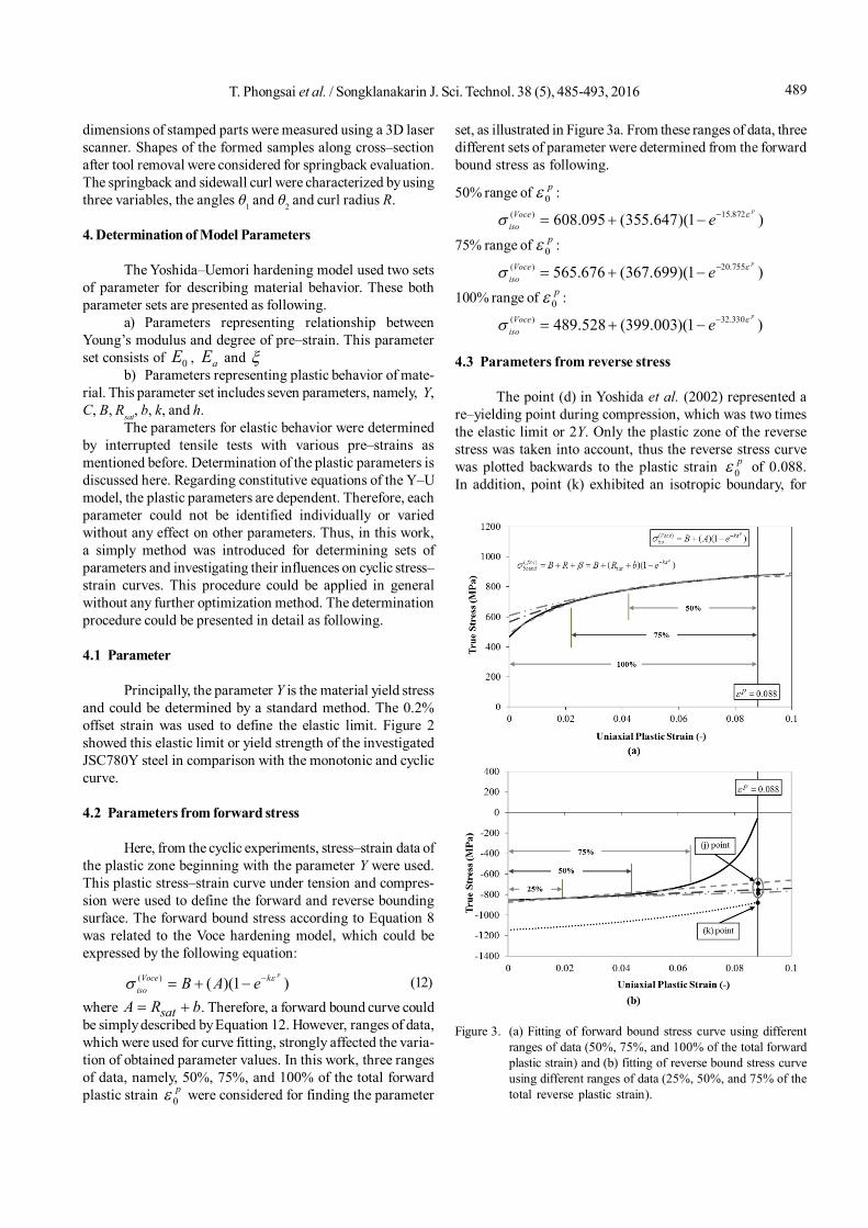
set, as illustrated in Figure 3a. From these ranges of data, threedifferent sets of parameter were determined from the forwardbound stress as following.

50% range of 0p :

( ) 15.872608.095 (355.647)(1 )pVoce

iso e

75% range of 0p :

( ) 20.755565.676 (367.699)(1 )pVoce

iso e

100% range of 0p :

( ) 32.330489.528 (399.003)(1 )pVoce

iso e

4.3 Parameters from reverse stress

The point (d) in Yoshida et al. (2002) represented are–yielding point during compression, which was two timesthe elastic limit or 2Y. Only the plastic zone of the reversestress was taken into account, thus the reverse stress curvewas plotted backwards to the plastic strain 0

p of 0.088.In addition, point (k) exhibited an isotropic boundary, for

Figure 3. (a) Fitting of forward bound stress curve using differentranges of data (50%, 75%, and 100% of the total forwardplastic strain) and (b) fitting of reverse bound stress curveusing different ranges of data (25%, 50%, and 75% of thetotal reverse plastic strain).

T. Phongsai et al. / Songklanakarin J. Sci. Technol. 38 (5), 485-493, 2016490

which value of the forward stress at a plastic strain of 0.088was used. For the investigated steel, the value of point (k)was about -876.12 MPa. Then, point (j) could be identifiedby an intersection of a linear extrapolation of the saturatedreverse stress with the plastic strain of 0.088. Three rangesof data of the reverse bound curve from the saturated pointwere incorporated, namely, 25%, 50%, and 75% of the totalreverse plastic strain, as shown in Figure 3b.

Following this, three values of point (j) in Yoshidaet al. (2002) were obtained for these different ranges of data:

25% range of 0p : value of point (j) was -777.87 MPa

50% range of 0p : value of point (j) was -752.36 MPa

75% range of 0p : value of point (j) was -684.71 MPa

Furthermore, the extrapolated line up to a deviationpoint of the reverse bound curve represented the region ofpermanent softening. The extrapolated line beyond thisregion until the total plastic strain described the transientBauschinger effect. They were used in conjunction with Equa-tion 9 to calculate the parameter b.

4.4 Parameter

Generally, in some literatures the parameter C wasdetermined by an optimization method. Such kind of methodwas sophisticated and expensive for industrial cases. On theother hand, solving for C from Equation 10 and 11 could beanother possibility. However, in this work more simplemethod for finding the parameter C was applied. The originalbackstress model as defined in Equation 13 was hereconsidered.

* *( )p pC a (13)

This was the principle equation before it was modified byYoshida et al. (2002) to be Equation 2. Thus, the value of Cwas then determined by a relation between cyclic tension–compression test data and parameter, as expressed in Equa-tion 14.

) ˆ( 2pC

Bt ae (14)

where ( )Bt described the differences between the reverse

stress-strain curve from the range (d)-(e) and the extrapolatedline of the transient Bauschinger region ((e)-(j)) in Yoshidaet al. (2002). ˆ p is the reverse plastic strain. Figure 4 showsthe proposed method for determining the parameter C. Bythis manner, a value of 92.037 was obtained for the parameterC. It was noticed that stress–strain curves obtained by thisvalue in the transient Bauschinger zone was acceptable whencomparing with experimental results.

4.5 Parameter h

In the literature, h is a material parameter, which was

used to adjust results of cyclic stress–strain curves obtainedfrom experiments and simulations. In this work, it was foundthat influence of the parameter h on the results of cyclicsimulations was small in the LS-DYNA solver. Therefore,a default value of h = 0.5 was taken into account.

From the procedures mentioned above, various para-meter sets were obtained and provided in Table 2. All sevenplastic parameters of the Y–U model for each range of fittingdata were presented. It was seen that the parameters could bequite different when the range of fitting data was varied. Theseparameter sets were further applied for FE simulations of 1–element model in order to investigate their effects on cyclicstress–strain responses.

5. FE Simulations

5.1 1-element model

FE simulations of tension–compression test wereperformed in LS-DYNA by using a single plane stress shellelement model. The model was a square element with a sizeof 1x1 mm. The left–bottom node was constrained in bothx– and y–direction, while the right–bottom node wasconstrained in the y–direction. Displacements in positive and

Figure 4. Determination of parameter C: (a) ( )Bt and (b) curve

fitting by Equation 14.

491T. Phongsai et al. / Songklanakarin J. Sci. Technol. 38 (5), 485-493, 2016

negative y–direction were applied to the top side of theelement. The element formulation type 2 (Belytschko-Tsay)with one integration point through thickness was used. Thiselement type was also further applied in forming simulations.Results of the each parameter set were compared with experi-mental data. Afterwards, averaged deviations between bothobtained stress–strain curves were calculated.

5.2 Forming simulation

In addition, numerical FE simulations of the hat–shape sample were carried out in LS-DYNA for predictingthe springback effect. It was also used to verify springbackresults of the parameter set, which was the best fit predictionof the cyclic stress–strain responses. The models of blankand tools were defined using shell elements and boundaryconditions were generated according to the experimentalsetup. A friction coefficient of 0.125 was given for everycontact surface. Calculated results were compared with theshape of the stamped part.

6. Results and Discussion

6.1 Cyclic stress–strain curves

To investigate influences of using different range offitting data, 1–element FE simulations were conducted withall parameter sets, given in Table 2. Some deviations of stress–strain curves from each parameter sets were observed. Thecyclic curves mainly differed at the beginning zone of forwardstress and around the saturation zone of reverse stress.When the data range of the forward stress was the same, butthe data range of the reverse stress increased, increases ofthe stress–strain curves in both tension and compressionregions were found. The whole cyclic curves seemed to shiftwhen only parameters from the reverse stress were altered.In case of using an increased data range of the forward stress,but the same data range of the reverse stress, decreases of

the forward stress were observed. Additionally, the calculatedcurves were compared with the experimental ones for anentire cycle and errors of each case were then determined.The mean differences and standard deviations for eachparameter sets were summarized in Table 3. It was found thatthe range of fitting data, which provided the best agreementwith the experimental data, was the 50% range of 0

p from theforward stress in combination with the 75% range of 0

p fromthe reverse stress (case C). The largest difference value wasnoticed by the 75% range of 0

p from the forward stress andthe 25% range of 0

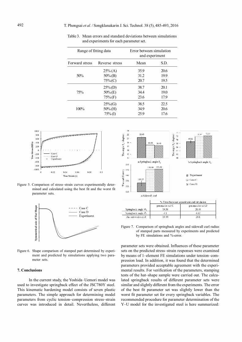
p from the reverse stress (case D). Thecyclic stress–strain curves of both parameter sets werecompared with the experimental curve in Figure 5. The worstparameter set exhibited significant lower forward stress, lowerreverse stress in the range of permanent softening and higherreverse stress in the transient Bauschinger region. For thebest parameter set, a maximum stress difference of 20 MPawas detected.

6.2 Springback results

To verify springback effects predicted by the Y–Umodel using the determined parameters, FE simulations ofhat–shape samples were carried out. Both parameter setsdiscussed before were applied to the simulations to investi-gate influences of model parameters on the calculated spring-back. Experimental and simulation results regarding bothdesignated angles 1 and 2, and sidewall curl radius R weredetermined. In Figure 6, dimensions of stamped parts obtainedfrom the experiment and predicted by the simulations usingtwo different parameter sets were compared. All three spring-back variables obtained from the experiments and predictedby the simulations were compared with resulted %-error inFigure 7. The calculated springback results of both parametersets were similar and slightly different from the experimentalone. Nevertheless, the error of the best fit parameter set wasslightly lower than the worst fit parameter set for everyspringback variable.

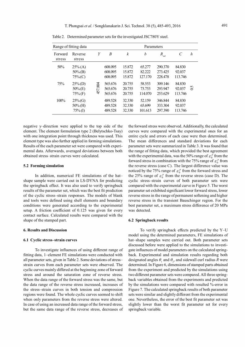
Table 2. Determined parameter sets for the investigated JSC780Y steel.

Range of fitting data Parameters

Forward Reverse Y B k b Rsat C hstress stress

50% 25% (A) 608.095 15.872 65.277 290.370 84.83050% (B) 608.095 15.872 82.222 273.425 92.03775% (C) 608.095 15.872 127.170 228.478 113.746

75% 25% (D) 565.676 20.755 58.553 309.146 84.83050% (E) 565.676 20.755 73.753 293.947 92.03775% (F) 565.676 20.755 114.070 253.629 113.746

100% 25% (G) 489.528 32.330 52.159 346.844 84.83050% (H) 489.528 32.330 65.699 333.304 92.03775% (I) 489.528 32.330 101.613 297.390 113.746

457.8

04

0.5

T. Phongsai et al. / Songklanakarin J. Sci. Technol. 38 (5), 485-493, 2016492

Figure 6. Shape comparison of stamped part determined by experi-ment and predicted by simulations applying two para-meter sets.

parameter sets were obtained. Influences of these parametersets on the predicted stress–strain responses were examinedby means of 1–element FE simulations under tension–com-pression load. In addition, it was found that the determinedparameters provided acceptable agreement with the experi-mental results. For verification of the parameters, stampingtests of the hat–shape sample were carried out. The calcu-lated springback results of different parameter sets weresimilar and slightly different from the experiments. The errorof the best fit parameter set was slightly lower than theworst fit parameter set for every springback variables. Therecommended procedure for parameter determination of theY–U model for the investigated steel is here summarized:

Figure 5. Comparison of stress–strain curves experimentally deter-mined and calculated using the best fit and the worst fitparameter sets.

Table 3. Mean errors and standard deviations between simulationsand experiments for each parameter set.

Range of fitting data Error between simulation and experiment

Forward stress Reverse stress Mean S.D.

25% (A) 35.9 20.650% 50% (B) 31.2 19.9

75% (C) 20.7 19.5

25% (D) 38.7 20.175% 50% (E) 34.4 19.0

75% (F) 23.6 17.9

25% (G) 38.5 22.5100% 50% (H) 34.9 20.6

75% (I) 25.9 17.6

7. Conclusions

In the current study, the Yoshida–Uemori model wasused to investigate springback effect of the JSC780Y steel.This kinematic hardening model consists of seven plasticparameters. The simple approach for determining modelparameters from cyclic tension–compression stress–straincurves was introduced in detail. Nevertheless, different

Figure 7. Comparison of springback angles and sidewall curl radiusof stamped parts measured by experiments and predictedby FE simulations and %-error.

493T. Phongsai et al. / Songklanakarin J. Sci. Technol. 38 (5), 485-493, 2016

1) Parameter Y was identified as the 0.2% offset yield stress,2) Forward bounding surface was obtained by fitting the50% range of the forward stress data and using the Vocehardening model, 3) Reverse bounding surface was deter-mined by fitting the 75% range of the reverse stress data andusing a linear equation, and 4) Parameter C was identified bythe differences between the reverse stress–strain curve andthe extrapolated line of the transient Bauschinger region.

Acknowledgements

Authors would like to acknowledge the NSTDA Uni-versity Industry Research Collaboration (NUI-RC) and theNational Research University Project of Thailand’s Office ofthe Higher Education Commission for financial support, theNational Metal and Materials Technology Center (MTEC),National Science and Technology Development Agency ofThailand (NSTDA) and Iron and Steel Institute of Thailand(ISIT) for the materials testing, Thai Marujun Co., Ltd. andChong Thai Rung Ruang Co., Ltd. for material support.

References

Armstrong, P.J. and Frederick, C.O. 1966. A mathematicalrepresentation of the multiaxial Bauschinger effect.G.E.G.B report RD/B/N 731

Carden, W.D., Geng, L.M., Matlock, D.K., and Wagoner, R.H.2002. Measurement of springback. InternationalJournal Mechanical Science. 44, 79-101.

Chongthairungruang, B., Uthaisangsuk, V., Suranuntchai, S.,and Jiratheranat, S. 2013. Springback prediction insheet metal forming of high strength steels. MaterialDesign. 50, 253-266

Collin, J.M., Parenteau, T., Mauvoisin, G., and Pilvin, P. 2009.Material parameters identification using experimentalcontinuous spherical indentation for cyclic harden-ing. Computational Materials Science. 46 (2), 333-338.

Eggertsen, P.A. and Mattiasson, K. 2010. On constitutivemodeling of springback analysis. International Journalof Mechanical Science. 52, 804-818.

Eggertsen, P.A. and Mattiasson, K. 2009. On constitutivemodeling of the bending-unbending behaviour foraccurate springback predictions. International Journalof Mechanical Science. 51, 547-563.

Gan, W. and Wagoner, R.H. 2004. Die design method forsheet springback. International Journal of MechanicalScience. 46, 1097-113.

Geng, L. and Wagone, R.H. 2000. Springback analysis witha modified hardening model. SAE paper No. 2000-01-0768, SAE. Inc.

Hodge, P.G. 1957. A new method of analyzing stresses andstrains in work hardening solids, Transactions ofASME. Journal of Applied Mechanics. 24, 482-483.

Kuwabara, T. 2007. Advances in Experiments on Metal Sheetsand Tubes in Support of Constitutive Modeling andForming Simulations. International Journal of Plastic-ity. 23, 385-419.

LS-DYNA, 2007. Keyword User’s Manual Version 971 Vol. 2:Material Models, Livermore Software TechnologyCorporation, California. USA.

Mattiasson, O.E. and Enqvist, B.K. 2006. Identification ofmaterial hardening parameters by the three-pointbending of metal sheets. International Journal ofMechanical Science. 48, 1525-1532.

Yoshida, F. and Uemori, T. 2002. A model of large-strain cyclicplasticity describing the Bauschinger effect and workhardening stagnation. International Journal of Plastic-ity. 18, 661-686.

Yoshida, F. and Uemori, T. 2003. A model of large-strain cyclicplasticity and its application to springback simulation.International Journal of Mechanical Science. 45, 1687-1702.

Yoshida, F., Uemori, T., and Fujiwara, K. 2002. Elastic-plasticbehaviour of steel sheets under in-plane cyclictension-compression at large strain. InternationalJournal of Plasticity, 18, 633-659.

Yoshida, F., Urabe, M., and Toropov, V.V. 1998. Identificationof material parameters in constitutive model for sheetmetals from cyclic bending tests. International Journalof Mechanical Science. 40, 237-249.

Zhao, K.M. and Lee, J.K. 2007. Generation of cyclic stress-strain curves for sheet metals. Journal of EngineeringMaterials Technology. 38, 391-395.