Identification of linear dynamic systems operating in a networked environment

This article appeared in a journal published by Elsevier. The attachedcopy is furnished to the author for internal non-commercial researchand education use, including for instruction at the authors institution

and sharing with colleagues.

Other uses, including reproduction and distribution, or selling orlicensing copies, or posting to personal, institutional or third party

websites are prohibited.

In most cases authors are permitted to post their version of thearticle (e.g. in Word or Tex form) to their personal website orinstitutional repository. Authors requiring further information

regarding Elsevier’s archiving and manuscript policies areencouraged to visit:

http://www.elsevier.com/copyright

Author's personal copy

Automatica 45 (2009) 2763–2772

Contents lists available at ScienceDirect

Automatica

journal homepage: www.elsevier.com/locate/automatica

Identification of linear dynamic systems operating in a networked environmentI

Jiandong Wang a, Wei Xing Zheng b,∗, Tongwen Chen ca Department of Industrial Engineering & Management, College of Engineering, Peking University, Beijing 100871, Chinab School of Computing & Mathematics, University of Western Sydney, Penrith South DC NSW 1797, Australiac Department of Electrical & Computer Engineering, University of Alberta, Edmonton, Alberta, Canada T6G 2V4

a r t i c l e i n f o

Article history:Received 2 January 2009Received in revised form8 June 2009Accepted 17 August 2009Available online 12 October 2009

Keywords:System identificationNetworked control systemsNon-synchronized non-uniformly sampleddata

a b s t r a c t

This paper studies a networked system identification problem, which aims at identifying mathematicalmodels required in networked control/estimation/filtering systems. Specifically, we consider the off-lineidentification of open-loop stable linear time-invariant processes working in a networked environment.In the networked environment, how the actuators (D/A conversion) operate plays a key role inthe complexity of the related identification problems. In particular, it is reasonable to consider theconfiguration of event-driven actuators subject to random network-induced delays and packet dropouts;as a result, the networked identification problem is formulated as the one to identify continuous-timelinear time-invariant models, based on the general non-uniformly non-synchronized sampled data. Amodified version of the simplified refined instrumental variablemethod is proposed to solve this problem,and is validated in a networked identification experiment based on the Matlab/Simulink simulatorTrueTime.

© 2009 Elsevier Ltd. All rights reserved.

1. Introduction

The last decade has witnessed an accelerated integration ofcommunication, computing networks and control systems at al-most all levels of operation and information processing in vari-ous areas, includingmanufacturing industry, remote operation andtele-autonomy (Hespanha, Naghshtabrizi, & Xu, 2007; Hokayem &Abdallah, 2004; Tipsuwan & Chow, 2003; Yang, 2006). Ever since,networked control/estimation/filtering systems have been verychallenging and promising research fields, and have receivedmuchattention from researchers and engineers; see, e.g., the special is-sues Antsaklis and Baillieul (2004, 2007), Bushnell (2001), Chow(2004) and Wang, Liu, Yang, and Li (2007) and numerous refer-ences therein.One of the distinguishing features for networked control/estim-

ation/filtering systems is data transmission over communicationnetworks. As a matter of fact, this feature is not a new concept.

I This research was partially supported by the National Natural ScienceFoundation of China under grant Nos. 60704031 and 10832006, by a Research Grantfrom the Australian Research Council, by the Natural Sciences and EngineeringResearch Council of Canada and by the 111 Project. The material in this paper wasnot presented at any IFAC meeting. This paper was recommended for publicationin revised form by Associate Editor Johan Schoukens under the direction of EditorTorsten Söderström.∗ Corresponding author. Tel.: +61 2 4736 0608; fax: +61 2 4736 0867.E-mail addresses: [email protected] (J. Wang), [email protected]

(W.X. Zheng), [email protected] (T. Chen).

From tele-operation for space and hazardous environment to pro-cess regulation with distributed control systems, for instance, datatransmission over communication networks has already been uti-lized for many years. These communication networks are usuallyspecialized and dedicated to ensure the timeliness of the trans-mission. However, with the trend of Ethernet, Internet, and wire-less networks becoming dominant, the networks are no longerspecialized and are often shared for various concurrent general-purposed applications (Eidson & Cole, 1998; Kaplan, 2001; Liu,Chai, Mu, & Rees, 2008; Moyne & Tilbury, 2007; Tang & de Silva,2006; Thompson, 2004; Yang, Chen, & Alty, 2003). As a result, theeffects of communication networks, e.g., network-induced delaysand packet dropouts, are too prominent to be ignorable in manyapplications, and need to be considered in the design and analysisof networked controllers/estimators/filters.This paper studies the problem of identifying mathematical

models of processes working in the networked environment, re-ferred to as the networked identification problem. Needless to say,the identified models are indispensably required in the networkedcontrol/estimation/filtering systems. To the best of our knowledge,this problem has received relatively low attention so far. Brscic,Petrovic, and Peric (2000) considered constant round-trip delaysand maximum delays, and performed an on-line identification ofdiscrete-time (DT) linear time-invariant (LTI) models using a re-cursive least-squares algorithm. Fei, Du, and Li (2008) introducedan actuator buffer to deal with the network non-deterministic fac-tors from the identifier to the actuator; by doing so, the problem isconverted into identification of DT LTI models with some missing

0005-1098/$ – see front matter© 2009 Elsevier Ltd. All rights reserved.doi:10.1016/j.automatica.2009.09.021

Author's personal copy

2764 J. Wang et al. / Automatica 45 (2009) 2763–2772

output data points (this is equivalent to Case I in Section 2.3 in thispaper).The contribution of this paper is two-fold. (i) A fundamental

question is addressed: what kind of identification problems arethere for an LTI process working in the networked environment?This is not an easy question to answer. To have a feasible start, welimit ourselves to the off-line identification of open-loop stable LTImodels. Under the effects of random network-induced delays andpacket dropouts, it is found out in this paper that the distinct run-ning modes of the actuator (D/A conversion) lead to several iden-tification problems with very different complexities. Consideringsome reasonable assumptions (Assumptions 1 and 2 in Section 2),we formulate the networked identification problemunder the con-figuration of event-driven actuators subject to random network-induced delays and packet dropouts. That is, a continuous-time(CT) LTI model is to be identified based on the general non-synchronized non-uniformly (NSNU) sampled data. (ii) To the bestof our knowledge, the CT model identification problem based ongeneral NSNU sampled data has seldom been considered in the lit-erature (see the literature survey in Section 3.2). Taking the mainidea of the simplified refined instrumental variable method for CTsystems (SRIVC), proposed by Young and his coworkers (Husel-stein & Garnier, 2002; Young, 2002, 2008; Young, Garnier, &Gilson, 2008; Young & Jakeman, 1980), amodified SRIVCmethod isproposed in this paper to solve the networked identification prob-lem. The proposed method is validated in a networked iden-tification experiment based on the Matlab/Simulink simulatorTrueTime (Cervin, Henriksson, Lincoin, Eker, & Arzen, 2003).The rest of the paper is organized as follows. Section 2 inves-

tigates the types of models to be identified, where two factorsare considered, namely, the effects of communication networksand the running modes of nodes in the network. Section 3 formu-lates a particular networked identification problem to be solvedin the rest of this paper. Section 4 proposes a modified versionof the simplified refined instrumental variable method to iden-tify CT LTI models based on the general NSNU sampled data. Sec-tion 5 presents a numerical example based on theMatlab/Simulinksimulator TrueTime to illustrate the effectiveness of the proposedmethod in solving the networked identification problem. Finally,some concluding remarks are given in Section 6.

2. Different models arisen in networked environments

This section starts with a brief description of the identificationproblem in the networked environment. Two factors, namely, theeffects of communication networks and the running modes ofnodes, are analyzed in detail to reach two types ofmodels includingsimple LTI models as well as complicated DT models which aretime-varying in parameters and in structures.

2.1. Problem description

Consider a CT LTI process working in a networked environmentdepicted in Fig. 1, where the timeline of the signals goes as follows.The process output y(t) for t ∈ R+ (the set of positive realnumbers) is sampled at the time instant tk by a sensor to yield aDT counterpart y(tk). The communication network transmits y(tk)to a remote computer that receives y(tk) at the time instant tl toproduce yc(tl). The computer, acting as an identification device,sends out a DT excitation input uc(tj) via the communicationnetwork at the time instant tj, which is received by an actuatorat the time instant ti to form u(ti). The actuator creates the CTinput u(t) based on u(ti) via zero-order hold (ZOH) to drive theprocess. Here the time instants tk, tl, tj and ti and their relationships

Sensor

Fig. 1. A diagram of a CT LTI process working in the networked environment.

a

b

c

d

e

Fig. 2. The timeline of signals in the networked environment: y(tk) and yc(tl) incircles, uc(tj) and u(ti) in squares, and y(t) and u(t) in solid lines.

dependon the effects of communicationnetworks, and the runningmodes of the sensor, the computer (identification device) and theactuator, and will be clarified later. Fig. 2 presents an illustrativeexample of these signals.We study the problem of identifying a CT model or a DT coun-

terpart of the process working in this networked environment,based on the available data yc(tl) and uc(tj) at the computer side. Inotherwords, identification is performed in a remotemanner via thecommunication network between the process and the computer.Henceforth, this problem is referred to as the networked identifi-cation problem. In particular, we limit ourselves to the off-line net-worked identification problem for open-loop stable LTI systems. InFig. 1, even though tjmaydependon tl (for an event-driven identifi-cation device), the value of uc(tj) is generated independent of yc(tl)so that an open-loop identification experiment is implemented.The problem studied in this paper could be a good starting pointto tackle the on-line networked identification problem for closed-loop systems, which may be practically more important, but morecomplicated.There are two factors which are distinctly different from the

standard identification problems, namely, the effects of commu-nication networks and the running modes of nodes in the networkincluding the sensor, computer and actuator. The two factors areinvestigated in Sections 2.2 and 2.3.

Author's personal copy

J. Wang et al. / Automatica 45 (2009) 2763–2772 2765

2.2. Effects of communication networks

We consider two major effects of communication networks,namely, network-induced delays and packet dropouts. With theincreasing usage of Ethernet, Internet andwireless communicationnetworks, these effects of communication networks are tooprominent to be ignorable in many applications.First, there are two network-induced delays in Fig. 1: τ ksc ∈ R

is the sensor-to-computer delay associated with y(tk), and τjca ∈ R

is the computer-to-actuator delay associated with uc(tj). The twodelays τ ksc and τ

jca are inevitable, due to limited bandwidth and

overhead in the network. In fact, they are sums of several smalldelays, including medium access delay, transportation delay, andcongestion delay. The characteristics of τ ksc and τ

jca can be constant

or random, depending on the network architectures, mediumaccess control protocols, operating conditions, and the chosenhardware. In many cases, especially for Ethernet, Internet andwireless communication networks, the delays are time-varying ina random fashion (Lian, Moyne, & Tilbury, 2002; Nilsson, 1998;Srinivasagupta, Schattler, & Joseph, 2004; Yang et al., 2003; Yang,2006; Zhang, Branicky, & Phillips, 2001). Hence, both τ ksc and τ

jca

here are assumed to be random, e.g., τ ksc and τjca in Fig. 2.

Second, data samples of y(tk) and uc(tj) may be lost/droppedwhile in transmission through the communication network. Thenetwork packet dropout is an inherent problem with most com-munication networks due to several factors such as node failure,transmission errors and buffer overflow resulting from congestion.Although network protocols are usually equipped with transmi-ssion-retry mechanisms, they can only re-transmit for a limited ti-me; after this time has expired, the packets are dropped (Hokayem& Abdallah, 2004; Zhang et al., 2001). The packet dropouts canbe modelled either as stochastic or deterministic phenomena(Hespanha et al., 2007), against which the proposed off-line iden-tification problem actually has no discrimination. Without loss ofgenerality, we assume that some random packet dropouts mayhappen at the sensor-to-computer side in Fig. 1, i.e., some samplesof y(tk) may be lost/dropped with a certain probability in the tra-nsmission. Similarly, the packet dropouts of uc(tj) at the compu-ter-to-actuator side may also happen; however, they have littleeffects on the open-loop identification owing to the fact that theZOH keeps its previous value if the update does not arrive. For ex-ample, y(2) and uc(5) in Fig. 2 are lost in the transmission.Therefore, we make the following assumption on the effects of

communication networks.

Assumption 1. The network-induced delays τ ksc and τjca are as-

sumed to be random within the range [0, τmax) for some real val-ued constant τmax; the communication network has a probabilityα (0 < α < 1) of packet dropouts in the transmission.

Note that both τmax and α are not required in the identification.In addition, τmax could be larger than the sampling period h thatis defined later to be associated with y(tk). The probability α canbe time-varying, which often occurs if the communication trafficvaries with time.

2.3. Running modes of the sensor, computer and actuator

The other factor different from the standard identification prob-lems is the running mode of the nodes including the sensor, com-puter and actuator. The running mode has two types, namely, theevent-driven running mode or the time-driven one.First, from a sampled-data system perspective, it is natural to

sample the process output y(t) equidistantly with a sampling pe-riod h ∈ R+. In other words, the sensor is in the time-driven run-ning mode, and y(tk) is uniformly sampled for tk = kh wherek ∈ Z+ (the set of positive integer), see, e.g., y(tk) in Fig. 2(a).

Second, the running mode of the computer, acting as the iden-tification device, does not really matter, because the identificationis performed in the off-line manner. Without loosing generality,the identification device is set to run in the event-driven mode:once y(tk) is received as yc(tl) by the computer, the identificationdevice transmits the excitation input uc(tj) out to the actuator viathe communication network; see, e.g., yc(tl) and uc(tj) in Fig. 2(b)and (c) respectively. However, the value of uc(tj) is independent ofyc(tl), i.e., it is an open-loop identification experiment. In addition,we ignore the computational delay in the computer and assumeuc(tj) to be sent out from the computer at the moment that yc(tl)is received, i.e., tj = tl.Finally, under Assumption 1, the two running modes for the

actuator lead to different types of models to be identified.

Case I: If the actuator is time-driven with updating period h, theCT input u(t) is piece-wise constant and is updated everyh time unit by taking the value of the latest updatedinput uc(tj), as shown in Fig. 2(d). The time-driven modecertainly requires the actuator having a buffer to store thereceived input uc(tj). If there are several updated samplesavailable within one sampling period, then all except thelatest one are discarded, e.g., the time interval [5h, 6h) inFig. 2(d). If no updating information is available withinone sampling period, the actuator adopts the strategy ofZOHandpreserves its previous value, e.g., the time interval[3h, 5h) in Fig. 2(d). For such a time-driven actuator, theCT input u(t) has no variation within one sampling period.If u(kh) and y(kh), the equidistantly sampled points ofu(t) and y(t) at the sampling instants kh respectively, canbe recovered, then we are facing a standard identificationproblem for a DT/CT LTI model.

Case II: If the actuator is event-driven, the CT input u(t)may expe-rience zero, one or multiple updates every h time unit dueto the randomnetwork-induced delays (Branicky, Phillips,& Zhang, 2000; Chow & Tipsuwan, 2001; Zhang et al.,2001). For instance, the time intervals [2h, 3h), [h, 2h), and[5h, 6h) in Fig. 2(e) have zero, one, and two variations, re-spectively. If the DT model is to be identified, then it istime-varying in parameters and in structures. This can beseen from the following example.

Example 1. Let the CT LTI process be in the state-spaceform,

dx(t)dt= Ax(t)+ Bu(t),

y(t) = Cx(t).

Suppose that the CT input u(t) always experiences onevariation within one sampling period h, i.e., one single up-dated excitation signal uc(tj) arrives at the actuator by atime instant ti = (k − 1)h + ∆k for some integer k ∈ Zand 0 < ∆k < h. By the step-invariant transformation(e.g., Chen and Francis (1995)), the DT model is

x((k+ 1)h) = Φx(kh)+ Γ0(∆k)u(kh)+Γ1(∆k)u((k− 1)h),

y(kh) = Cx(kh),

where

Φ = eAh, Γ0(∆k) =

∫ h−∆k

0eAtdt · B,

Γ1(∆k) =

∫ h

h−∆keAtdt · B.

The DT model also can be written in the transfer functionform as

Author's personal copy

2766 J. Wang et al. / Automatica 45 (2009) 2763–2772

y(kh) = C(I − qΦ)−1Γ0(∆k)u(kh)+ C(I − qΦ)−1Γ1(∆k)u((k− 1)h)

=:B0(q; k)A(q)

u(kh)+B1(q; k)A(q)

u((k− 1)h).

In general, there are perhapsm variations within one sam-pling period h; thus, the DT model containsm+ 1 delayedinputs with different numerator parameters. Since m and∆k are time-varying due to the random network-induceddelays, the DT model is time-varying in parameters and instructures. �

Identification of the DT model, being time-varying in pa-rameters and in structures, would be very difficult. How-ever, note that the time-varying nature is purely causedby the event-driven running mode of the actuator and therandom network-induced delays, even though the under-lying CT process is LTI. Therefore, it would bemore reason-able to study the networked identification problem in theCT domain, i.e., the objective is to identify a CT LTI modelbased on the DT samples y(tk) and u(ti).

The selection of the running mode for the actuator deserves afurther discussion here. The introduction of a buffer in the time-driven actuator implies some extra waiting time required, that is,the waiting for the next actuator equidistantly-spaced updatinginstant to arrive before the process input can be updated. In otherwords, we sometimes are using earlier information than we needto (see Fig. 2(d)). This can lead to a degradation of performance,in particular for networked control systems, in comparison withan event-driven actuator. Thus, event-driven actuators are usuallypreferred to time-driven ones (Nilsson, 1998; Yang, 2006).As a summary, we make the following assumption on the run-

ning modes of the sensor, computer and actuator.

Assumption 2. The sensor is time-driven with sampling periodh ∈ R+ time unit. The identification device in the computeris event-driven, sending out uc(tj) at the moment of receivingyc(tl); however, the value of uc(tj) is generated in advance beforethe identification experiment, being independent of yc(tl). Theactuator is in the event-driven running mode of updating u(t) atthe moment ti when uc(tj) is received as u(ti).

3. Formulation of a networked identification problem

As discussed in Section 2, it is reasonable to consider the net-worked identification problem under Assumptions 1 and 2 in theCT domain. This section first discusses the recovery of the processinput u(ti) and process output y(tk), under the help of the time-stamping technique. Next, a networked identification problem isformulated, i.e., a CT LTI model is to be identified based on theNSNU sampled data.

3.1. Recovery of the process input and process output

The networked identification problem needs to recover theprocess input u(ti) and process output y(tk) in order to identify theprocess parameters, based on the available data yc(tl) and uc(tj) atthe computer side.To do so, we need to measure the information of network-

induced delays and packet dropouts. This can be achieved by theso-called time-stamping technique. The transmitted output y(tk)is marked with the time when it was generated. Once the packetincluding y(tk) and its time stamp is received at the computer, thesensor-to-computer delay τ ksc is calculated by comparing the timestamp of y(tk) with the internal clock of the computer. Similarly,the actuator node can calculate the computer-to-actuator delay τ jcaassociatedwith uc(tj) and tj sent by the computer. The information

of τ jca can be available to the computer in two ways. One wayis to immediately send a message containing τ jca back from theactuator to the computer, while the other way is to pass τ jca onto the sensor and to include τ jca in the next sensor-to-computerdata packet (Nilsson, 1998; Tang & de Silva, 2006). Certainly, theactuator is assumed here to be capable of additional computation(to calculate τ jca) and communication (to send τ

jca to the computer

or to pass on it to the sensor). In most networks, the extra networkload introduced by transmitting the time stamps or the network-induced delays is negligible in comparison with the load oftransmitting signals and the network overhead. It is worthy to notethat the time-stamping technique requires clock synchronization(being a research area in itself) in all nodes of the communicationnetwork, which can be achieved via the software synchronizationor the hardware synchronization (Nilsson, 1998; Yang, 2006);see e.g. Faizulkhakov (2007), Ishikawa and Mita (2008) and Su(2008) for the state-of-the-art clock synchronization techniques.The time-stamping technique also needs the sequence numberingtechnique to assign a sequence number for each packet; otherwise,the time stamp alone cannot tell whether a packet is lost ornot (see e.g. Forouzan (2007) (Pages 318 and 915 therein)). As amatter of fact, the time-stamping technique has been exploitedin many studies of networked control systems, e.g., Lian et al.(2002), Nilsson (1998), Srinivasagupta et al. (2004) and Tang andde Silva (2006). Hence, wemake an assumption on using the time-stamping technique.

Assumption 3. The time-stamping technique is used for all thedata transmission.

Under Assumption 3, both the process input u(ti) and processoutput y(tk) can be completely recovered, based on the data pointsof yc(tj) and uc(tl) collected at the computer side, the informationof τ ksc and τ

jca, the runningmodes of the sensor, computer and actu-

ator, and the ZOH property of the actuator. The recovery certainlyis not available at the moment of ti or tk, but is done after waitingfor a certain period of time to receive all the required information;this is normally not a problem for the off-line identification here.In particular, y(tk) is recovered from the received packet con-

taining the values and time stamp of y(tk). Here tk = kh withk ∈ Z+ because the sensor is in the time-driven running mode.At the ending stage of data collection, if the value and time stampof y(tk) at tk = kh are not received due to packet dropouts, y(tk)cannot be recovered and is regarded as the missing data.The value of uc(tj), its transmission status of being success or

failure, and the associated computer-to-actuator delay τ jca tell usthe full information of u(ti). Here the transmission status of uc(tj)is known to its sender computer, sincemost transmission protocolshave the mechanism to provide this information. However, thereis one exceptional scenario where u(ti) cannot be recovered. Aspreviously discussed, τ jca is transmitted back to the computer viaeither side of the communication channels. If the packet containingτjca is dropped in the transmission, and the corresponding uc(tj) hasa success transmission status, there will be no way of recoveringthe corresponding input u(ti). This exceptional scenario can betreated the same as the case that u(t) is taking the value of thelast received input sample u(ti−1) without a new update; such atreatment inevitably introduces errors. To simplify the discussion,we ignore this exceptional scenario in what follows and leave it forfuture studies.

3.2. Non-synchronized non-uniformly (NSNU) sampled data

Let us take a closer look at u(ti) and y(tk). Besides the illustrativeexample in Fig. 2, a typical example of y(tk) and u(ti) from Section 5is shown in Fig. 3.

Author's personal copy

J. Wang et al. / Automatica 45 (2009) 2763–2772 2767

a

b

Fig. 3. An example of y(tk) and u(ti).

First, y(tk) is uniformly sampled formost of time, except at someinstants where the data points are missed owing to the dropoutof the packets containing y(tk). Second, u(ti) is completely non-uniformly sampled, due to the randomnetwork-induced delays; inaddition, the intersample behavior of u(ti) is piece-wise constantbecause of the ZOH. As a result, the sampling patterns of u(ti) andy(tk) can be regarded as general non-synchronized non-uniformly(NSNU) sampled data, i.e., both the input and output are non-uniformly sampled, and they do not have to be synchronized. Itis worthy to point out that the sensor does not have to work inthe time-driven mode, i.e., the CT output y(t) can be sampled in anon-periodic fashion (Hespanha et al., 2007); in this case, y(tk) ingeneral is non-uniformly sampled.To the best of our knowledge, the NSNU sampled data is seldom

considered in the literature of CT model identification (Garnier &Wang, 2008). The most relevant work is based on non-uniformlysampled but synchronized data. Tsang and Billings (1995) stud-ied the identification of CT model from non-uniformly sampleddata via a state variable filter with the key step of adapting theEuler method or Runge–Kutta method for non-uniformly sam-pled data. Huselstein and Garnier (2002), Young (2002) and Younget al. (2008) discussed the capability of applying the simplifiedrefined instrumental variable method for non-uniformly sampleddata. Larsson, Mossberg, and Soderstrom (2007, 2008) devised adiscrete approximation of the differentiation operator for CTmodelidentification and extended the derivative approximation to han-dle the case of irregular sampling. Ahmed, Huang, and Shah (2008)took the linear filter method to provide the unmeasurable deriva-tives and estimated the timedelay and systemparameters simulta-neously from the non-uniformly sampled data. In these referencesand examples presented therein, both the output and input arenon-uniformly sampled, but are synchronized, i.e., tk is not evenly-spaced and ti is the same as tk in the current context. Even thoughsome of the above methods have the potential of being applica-ble to the NSNU sampled data y(tk) and u(ti) here, none of themhave indeed considered this particular sampling pattern arisen inthe networked environment.To be precise, the networked identification problem is stated as

follows: Given the recovered non-uniformly sampled output y(tk) fortk ∈ R+, and the non-uniformly sampled input u(ti) for ti ∈ R+ withthe piece-wise constant intersample behavior, identify in an off-linemanner the asymptotically stable CT model working in an open-loopoperation. Note that y(tk) and u(ti) are not synchronized, i.e., tk ingeneral is different from ti.

4. The modified SRIVC method

Among the related work mentioned in Section 3.2, the SRIVCmethod proposed by Young and his coworkers (Huselstein &Garnier, 2002; Young, 2002, 2008; Young et al., 2008; Young &Jakeman, 1980), referred to as the original SRIVC method in whatfollows, has been successfully validated via numerical andpracticalexamples over years. This method is implemented by the function‘‘srivc’’ in the latest version of CONTSID toolbox (Garnier, Gilson,Bastogne, & Mensler, 2008) (available at http://www.cran.uhp-nancy.fr/contsid/), and can be applied for non-uniformly sampledbut synchronized input and output data. Taking the main idea ofthe original SRIVC method, we propose a modified SRIVC methodthat can deal with the general NSNU sampled data.

4.1. Problem formulation

Let the CT LTI process in Fig. 1 be described by a constant coef-ficient differential-delay equation,

dnx(t)dtn

+ a1dn−1x(t)dtn−1

+ · · · + anx(t)

= b0dmu(t − τ)dtm

+ · · · + bmu(t − τ). (1)

The ordersm and n (n ≥ m for a proper model), as well as the timedelay τ between x(t) and u(t), are assumed to be known a priori;otherwise, they can be determined together with the parameterestimation, e.g., in the samemanner as that in Section 4.6 of Younget al. (2008). In what follows, τ is ignored to simplify the notation.By ignoring τ and taking p as the differential operator, i.e.,

pix(t) =dix(t)dt i

,

Eq. (1) is rewritten in a compact transfer function form

x(t) = G(p)u(t) =B(p)A(p)

u(t), (2)

with

B(p) = bopm + b1pm−1 + · · · + bm,A(p) = pn + a1pn−1 + · · · + an.Here A(p) and B(p) are assumed to be coprime, and G(p) is asymp-totically stable. Consider an additive noise e(t) corrupting x(t) toyield the outputmeasurement y(t), i.e., y(t) = x(t)+e(t). If y(t) isnon-uniformly sampled to yield y(tk), i.e., tk is not evenly-spaced,then e(tk) is the noise associated with y(tk),y(tk) = x(tk)+ e(tk). (3)For the moment, assume that e(tk) is a DT Gaussian white noisewith zero mean and variance σ 2e ; the colored noise case will bediscussed later in Sections 4.2 and 4.3. The maximum likelihoodestimate of e(tk) is given byε(tk) = y(tk)− x(tk)

= y(tk)−B(p)A(p)

u(ti). (4)

Here the expression x(tk) =B(p)A(p)u(ti) stands for the operation of

sampling at the time instant tk the output of the CT filter B(p)/A(p)driven by the CT counterpart of u(ti). Note that u(ti) is availablehere instead of u(tk). Since the polynomial operator commutes inthe linear case, (4) becomes

ε(tk) =1A(p)

(A(p)y(tk)− B(p)u(ti))

=: A(p)yf (tk)− B(p)uf (tk), (5)where

Author's personal copy

2768 J. Wang et al. / Automatica 45 (2009) 2763–2772

yf (tk) :=1A(p)

y(tk), uf (tk) :=1A(p)

u(ti).

Eq. (5) yields a linear regression model,

y(n)f (tk) = ϕTf (tk)θ + ε(tk), (6)

where

ϕf (tk) =[−y(n−1)f (tk), −y

(n−2)f (tk), . . . , −yf (tk),

u(m)f (tk), u(m−1)f (tk), . . . , uf (tk)]T,

θ =[a1, a2, . . . , an, b0, b1, . . . , bm

]T.

Here y(i)(t) or u(i)(t) denotes the ith time derivative of the CT signaly(t) or u(t). The procedure of obtaining the filtered signals yf (tk)and uf (tk) and their derivatives y

(n)f (tk), y

(n−1)f (tk), . . . , y

(1)f (tk) and

u(m)f (tk), u(m−1)f (tk), . . . , u

(1)f (tk) will be addressed later in Sec-

tion 4.2. The identification problem can now be stated as follows:Given the collected data u(ti) and y(tk), identify the parametervector θ .

4.2. Identification algorithm

We propose a modified SRIVC method for the general NSNUsampled data in the networked environment. The main idea is tointroduce an iteration between estimating the parameter θ basedon (6) by the instrumental variable method (IVM), and updatingthe instrumental variable generated by an auxiliary model basedon the previous estimated parameter.A modified SRIVC method for the NSNU sampled Data:Stage A. Initialization:

A1. Design a filter

fc(p) =1

(p+ λ)n, (7)

where λ ∈ R is chosen so that it is equal to or larger than thebandwidth of G(p). Note that n ≥ m so that the order of fc(p)is set to be n, and the knowledge of the bandwidth of G(p) isassumed to be known a priori, or can be obtained via some pre-liminary tests such as step tests that are normally performedbefore designing identification experiments in practice (seee.g., Section 3.2 of Zhu (2001)).

A2. Filter y(tk) via the CT filter fc(p) and sample the resultingsignal and its derivatives at tk as an estimation of y

(n)f (tk),

y(n−1)f (tk), . . . , yf (tk). In the filtering operation (see Fig. 5), theintersample behavior of y(tk) is not available and y(tk) is in-terpolated in a first-order hold (FOH) fashion to obtain the CTcounterpart y(t).

A3. Filter u(ti) via the CT filter fc(p) and sample the resultingsignal and its derivatives at tk as an estimation of u

(m)f (tk),

u(m−1)f (tk), . . . , uf (tk). Owing to the ZOH, u(ti) is known tohave the piece-wise constant intersample behavior to form theCT counterpart u(t).

A4. Use the least-squares method to obtain an initial estimate θ0of θ based on (6), i.e.,

θ0 =

(N∑k=1

ϕf (tk)ϕTf (tk)

)−1 N∑k=1

ϕf (tk)y(n)f (tk).

Stage B. Iterative estimation: for j = 1 : convergence

B1. Generate the estimates of the noise-free output x(t) that aresampled at the time instants tk and t∆, denoted as x(tk,∆), basedon the previous estimate θj−1 and u(ti), i.e.,

x(tk,∆) =B(p, θj−1)

A(p, θj−1)u(ti). (8)

Once again, u(ti) takes the piece-wise constant intersamplebehavior owing to the ZOH. Here the time index t∆ is evenly-spaced with a small incremental step comparing with thesampling period h.

B2. Filter y(tk), u(ti) and x(tk,∆) via a CT filter fc(p) = 1/A(p, θj−1)and sample the resulting signals and their derivatives at tk toreach

Yf(tk) :=[y(n)f (tk), y

(n−1)f (tk), . . . , yf(tk)

]T,

Uf(tk) :=[u(m)f (tk), u

(m−1)f (tk), . . . , uf(tk)

]T,

Xf(tk) :=[x(n)f (tk), x

(n−1)f (tk), . . . , xf(tk)

]T.

In the filtering operation, the intersample behaviors of y(tk)and x(tk,∆) are not available; both are interpolated in anFOH fashion. By contrast, u(ti) has the piece-wise constantintersample behavior owing to the ZOH.

B3. Use the IVM to obtain the updated estimate θj,

θj =

(N∑k=1

ϕf (tk)ϕTf (tk)

)−1 N∑k=1

ϕf (tk)y(n)f (tk). (9)

Here the instrumental variable ϕf (tk) is the noise-freecounterpart of ϕf (tk) where y

(l)f (tk) for l = 0, 1, . . . , n − 1

are replaced by the estimate x(l)f (tk) of the noise-free outputx(l)f (tk), i.e.,

ϕf (tk) =[−x(n−1)f (tk), −x

(n−2)f (tk), . . . , −xf (tk),

u(m)f (tk), u(m−1)f (tk), . . . , uf (tk)]T. (10)

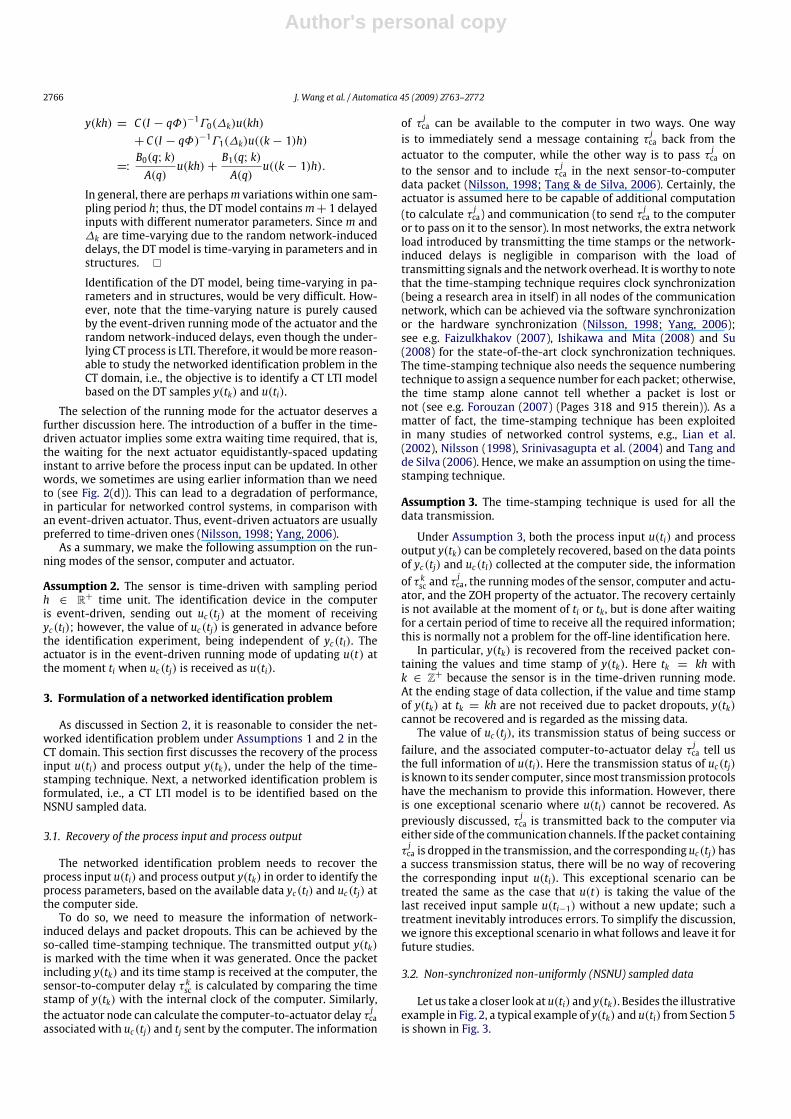
endThe steps in Stage B are diagrammatically illustrated in Fig. 4.

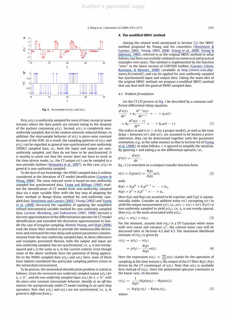
In particular, the filtering operation is one of the kernel steps,and deserves a detailed illustration. Taking yf (tk) := 1

A(p)y(tk)for instance, the filtering by 1/A(p) plays two roles of genera-ting the filtered output yf (tk) and its derivatives y

(n)f (tk), y

(n−1)f (tk),

. . . , y(1)f (tk) required in (6), and of improving the estimation qual-ity of θ . The required filtering operation can be implemented bysampling the solution of the state-space model in (11) driven byy(tk):[y(n)f (t), y(n−1)f (t), . . . , y(1)f (t)

]T

=

−a1 −a2 · · · −an1 0 · · · 0...

. . .. . .

...0 · · · 1 0

y(n−1)f (t)y(n−2)f (t)

...yf (t)

+10...0

y(t). (11)

Here the intersample behavior of y(tk) is not available and y(tk)has to be interpolated in some manner (e.g., by taking the FOHintersample behavior) to obtain the CT counterpart y(t). If thediscretization interval used in the numerical integration is shortcomparing with the averaged sampling interval of y(tk), which isusually the case, then the error induced could be tolerable. Thisimplementation is graphically illustrated in Fig. 5.The filtering operation uf (tk) := 1

A(p)u(ti) is implemented

in the same way to obtain uf (tk) and its derivatives u(m)f (tk),

Author's personal copy

J. Wang et al. / Automatica 45 (2009) 2763–2772 2769

Fig. 4. The filtered signals yf (t), uf (t), xf (t), and their derivatives.

Fig. 5. The filtered output yf (t) = y(t)/A(p) and its derivatives (This figure is basedon Figure 4.1 in Young et al. (2008)).

u(m−1)f (tk), . . . , uf (tk). Note that unlike y(tk), the intersample be-havior of u(ti) is piece-wise constant owing to the ZOH, so that theinterpolation error does not exist.Besides yf (tk) and uf (tk) and their derivatives, the modified

SRIVC method also requires the estimates of x(n−1)f (tk), x(n−2)f (tk),

. . . , xf (tk) in (9). The estimation process involves two filteringoperations in steps B1 and B2, which can be implemented in asimilarway as the filtering operation for yf (tk) and its derivatives. Aspecial treatment is to introduce the time index t∆ alongwith ti andtk. By doing so, we can reduce the interpolation error of formingthe CT noise-free output x(t) based on its discrete sample x(tk,∆) instep B2 to obtain Xf(tk), and can significantly improve the accuracyof the parameter estimation. Note that steps B1 and B2 cannot belumped together, because x(n−1)f (tk), x

(n−2)f (tk), . . . , x

(1)f (tk) need to

be obtained in step B2.Up until now, e(tk) has been assumed to be a white noise, for

which the proposed modified SRIVC method yields an efficientestimate of θ (to be clarified in Section 4.3). If e(tk) is colored, theresulting estimate of θ is still unbiased and consistent, owing to theindependence nature between e(tk) and the instrumental variableϕf (tk) that is solely correlated to the input u(ti). However, in thiscase, the parameter estimates are no longer efficient; finding amore effective method is left for future research.

4.3. Theoretical analysis

This section analyzes the convergence of the proposedmodifiedSRIVC method, as well as the optimality and asymptotic distribu-tion of the resulting parameter estimates.Before starting the theoretical analysis, we need to clarify the

relationship between the modified SRIVC method and the originalone. The modified SRIVC method shares the same fundamen-tal idea with the original SRIVC method, but has two differences:(i) The modified SRIVC method explicitly considers the general

NSNU sampled I/O data u(ti) and y(tk), while the original SRIVCmethod cannot be applied to this special sampling patternwithoutproper changes. (ii) Besides ti and tk, the time index t∆ is introducedin order to reduce the interpolation error in the filtering operationin step B2 to obtain Xf(tk). By doing so, the accuracy of the para-meter estimation can be improved significantly.Because of the above relationship, the modified SRIVC method

inherits from the original SRIVC method the same theoreticalresults. In terms of convergence, Section 4.1 of Young (2008) orSection 4.4.2 of Young et al. (2008) has already provided somepreliminary analysis for the original SRIVC method by noticing thesimilaritywith the iterative least-squares algorithmof Steiglitz andMcBride (1965). In fact, the original SRIVCmethod shares the samespirit with the bootstrap IV-based estimator BE1 in Söderström andStoica (1983) (Page 38 therein), the convergence of which has beenestablished under mild conditions by Theorem 4.5 in Söderströmand Stoica (1983). Thus, the local convergence of the modifiedSRIVC method can be established analogously.In terms of the consistency, because themodified SRIVCmethod

exploits the mechanism of using instrumental variables to elim-inate noise effects, the converging estimate θj in (9) is asymptoti-cally unbiased and consistent, i.e., θj → θ as the data lengthN goesto infinity. For optimality, if the additive noise is white, the originalSRIVCmethod is known to perform optimally (Young, 2008; Younget al., 2008; Young & Jakeman, 1980), i.e., the parameter estimatesconverge on themaximum likelihood estimates and are asymptot-ically efficient. This optimality result holds for the modified SRIVCmethod, too. In particular, we have the following asymptotic prop-erty for the parameter estimates.

Theorem 1. If the CT LTI model G(p) in (2) is stable and identifiable,the noise e(tk) in (3) is independent and identically distributed withzero mean and variance σ 2, and the input u(tk) is persistently excitedand is independent of e(tk), then the parameter estimate θj in (9)obtained by the modified SRIVC method is asymptotically normal-distributed (abbreviated as AsN), i.e.,

(θj − θ) ∈ AsN(0, Pθj).

Here the covariance matrix of the parameter estimation error is

Pθj =σ 2

N

[limN→∞

1N

N∑t=1

ϕf (tk)ϕTf (tk)

]−1, (12)

where ϕf (tk) is the noise-free version of the vector ϕf (tk) in (6),

ϕf (tk)

=

[−x(n−1)f (tk), . . . , −xf (tk), u

(m)f (tk), . . . , uf (tk)

]T.

Proof of Theorem 1. It is followed in the same manner as thecounterpart of the original SRIVCmethod, see e.g., the proof of The-orem 4.1 in Young et al. (2008). �

After the iterative estimation of Stage B in Section 4.2 com-pletes, the covariance matrix Pθ associated with the converged es-timate θj can be estimated as

Pθj = σ2

[N∑t=1

ϕf (tk)ϕTf (tk)

]−1, (13)

where ϕf (tk) is the instrumental variable in (10) associatedwith θj,and σ 2 is the variance of the residual estimate,

ε(tk) = y(tk)− x(tk)

= y(tk)−B(p, θj)

A(p, θj)u(ti).

Thus, Pθj in (13) provides the estimate of the uncertainty in the

Author's personal copy

2770 J. Wang et al. / Automatica 45 (2009) 2763–2772

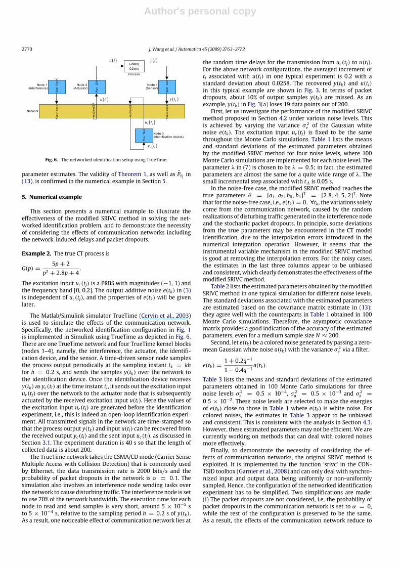
Fig. 6. The networked identification setup using TrueTime.

parameter estimates. The validity of Theorem 1, as well as Pθj in(13), is confirmed in the numerical example in Section 5.

5. Numerical example

This section presents a numerical example to illustrate theeffectiveness of the modified SRIVC method in solving the net-worked identification problem, and to demonstrate the necessityof considering the effects of communication networks includingthe network-induced delays and packet dropouts.

Example 2. The true CT process is

G(p) =5p+ 2

p2 + 2.8p+ 4.

The excitation input uc(tj) is a PRBS with magnitudes (−1, 1) andthe frequency band [0, 0.2]. The output additive noise e(tk) in (3)is independent of uc(tj), and the properties of e(tk) will be givenlater.

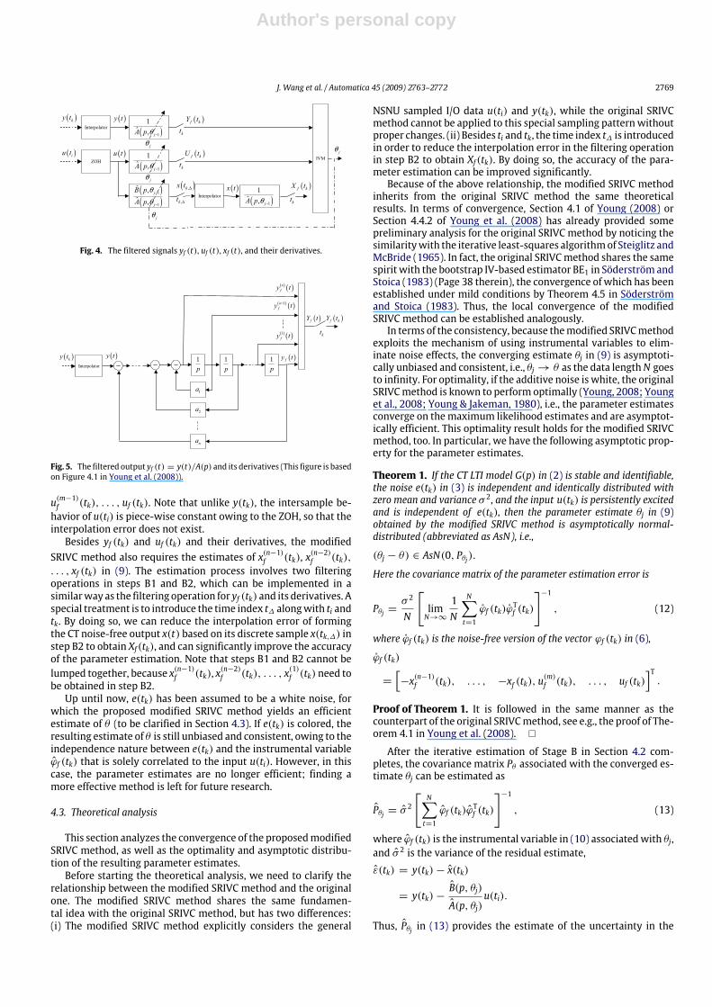
The Matlab/Simulink simulator TrueTime (Cervin et al., 2003)is used to simulate the effects of the communication network.Specifically, the networked identification configuration in Fig. 1is implemented in Simulink using TrueTime as depicted in Fig. 6.There are one TrueTime network and four TrueTime kernel blocks(nodes 1–4), namely, the interference, the actuator, the identifi-cation device, and the sensor. A time-driven sensor node samplesthe process output periodically at the sampling instant tk = khfor h = 0.2 s, and sends the samples y(tk) over the network tothe identification device. Once the identification device receivesy(tk) as yc(tl) at the time instant tl, it sends out the excitation inputuc(tj) over the network to the actuator node that is subsequentlyactuated by the received excitation input u(ti). Here the values ofthe excitation input uc(tj) are generated before the identificationexperiment, i.e., this is indeed an open-loop identification experi-ment. All transmitted signals in the network are time-stamped sothat the process output y(tk) and input u(ti) can be recovered fromthe received output yc(tl) and the sent input uc(tj), as discussed inSection 3.1. The experiment duration is 40 s so that the length ofcollected data is about 200.The TrueTime network takes the CSMA/CDmode (Carrier Sense

Multiple Access with Collision Detection) that is commonly usedby Ethernet, the data transmission rate is 2000 bits/s and theprobability of packet dropouts in the network is α = 0.1. Thesimulation also involves an interference node sending tasks overthe network to cause disturbing traffic. The interference node is setto use 70% of the network bandwidth. The execution time for eachnode to read and send samples is very short, around 5 × 10−5 sto 5 × 10−4 s, relative to the sampling period h = 0.2 s of y(tk).As a result, one noticeable effect of communication network lies at

the random time delays for the transmission from uc(tj) to u(ti).For the above network configurations, the averaged increment ofti associated with u(ti) in one typical experiment is 0.2 with astandard deviation about 0.0258. The recovered y(tk) and u(ti)in this typical example are shown in Fig. 3. In terms of packetdropouts, about 10% of output samples y(tk) are missed. As anexample, y(tk) in Fig. 3(a) loses 19 data points out of 200.First, let us investigate the performance of the modified SRIVC

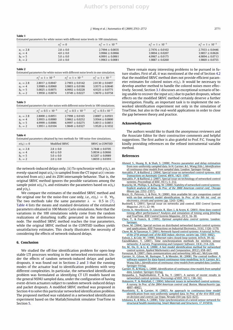
method proposed in Section 4.2 under various noise levels. Thisis achieved by varying the variance σ 2e of the Gaussian whitenoise e(tk). The excitation input uc(tj) is fixed to be the samethroughout the Monte Carlo simulations. Table 1 lists the meansand standard deviations of the estimated parameters obtainedby the modified SRIVC method for four noise levels, where 100Monte Carlo simulations are implemented for each noise level. Theparameter λ in (7) is chosen to be λ = 0.5; in fact, the estimatedparameters are almost the same for a quite wide range of λ. Thesmall incremental step associated with t∆ is 0.05 s.In the noise-free case, the modified SRIVC method reaches the

true parameters θ = [a1, a2, b0, b1]T = [2.8, 4, 5, 2]T. Notethat for the noise-free case, i.e., e(tk) = 0, ∀tk, the variations solelycome from the communication network, caused by the randomrealizations of disturbing traffic generated in the interference nodeand the stochastic packet dropouts. In principle, some deviationsfrom the true parameters may be encountered in the CT modelidentification, due to the interpolation errors introduced in thenumerical integration operation. However, it seems that theinstrumental variable mechanism in the modified SRIVC methodis good at removing the interpolation errors. For the noisy cases,the estimates in the last three columns appear to be unbiasedand consistent, which clearly demonstrates the effectiveness of themodified SRIVC method.Table 2 lists the estimated parameters obtained by themodified

SRIVC method in one typical simulation for different noise levels.The standard deviations associated with the estimated parametersare estimated based on the covariance matrix estimate in (13);they agree well with the counterparts in Table 1 obtained in 100Monte Carlo simulations. Therefore, the asymptotic covariancematrix provides a good indication of the accuracy of the estimatedparameters, even for a medium sample size N ≈ 200.Second, let e(tk) be a colored noise generated by passing a zero-

mean Gaussian white noise a(tk)with the variance σ 2e via a filter,

e(tk) =1+ 0.2q−1

1− 0.4q−1a(tk).

Table 3 lists the means and standard deviations of the estimatedparameters obtained in 100 Monte Carlo simulations for threenoise levels σ 2a = 0.5 × 10−4, σ 2a = 0.5 × 10−3 and σ 2a =0.5 × 10−2. These noise levels are selected to make the energiesof e(tk) close to those in Table 1 where e(tk) is white noise. Forcolored noises, the estimates in Table 3 appear to be unbiasedand consistent. This is consistent with the analysis in Section 4.3.However, these estimated parameters may not be efficient. We arecurrently working on methods that can deal with colored noisesmore effectively.Finally, to demonstrate the necessity of considering the ef-

fects of communication networks, the original SRIVC method isexploited. It is implemented by the function ‘srivc’ in the CON-TSID toolbox (Garnier et al., 2008) and can only deal with synchro-nized input and output data, being uniformly or non-uniformlysampled. Hence, the configuration of the networked identificationexperiment has to be simplified. Two simplifications are made:(i) The packet dropouts are not considered, i.e, the probability ofpacket dropouts in the communication network is set to α = 0,while the rest of the configuration is preserved to be the same.As a result, the effects of the communication network reduce to

Author's personal copy

J. Wang et al. / Automatica 45 (2009) 2763–2772 2771

Table 1Estimated parameters for white noises with different noise levels in 100 simulations.

σ 2e = 0 σ 2e = 1× 10−4 σ 2e = 1× 10

−3 σ 2e = 1× 10−2

a1 = 2.8 2.8± 0.0 2.7994± 0.0035 2.7976± 0.0102 2.7933± 0.0446a2 = 4 4.0± 0.0 3.9966± 0.0066 3.9894± 0.0207 3.9857± 0.0626b0 = 5 5.0± 0.0 4.9991± 0.0061 4.9967± 0.0175 4.9894± 0.0713b1 = 2 2.0± 0.0 1.9963± 0.0081 1.9887± 0.0260 1.9869± 0.0755

Table 2Estimated parameters forwhite noiseswith different noise levels in one simulation.

σ 2e = 1× 10−4 σ 2e = 1× 10

−3 σ 2e = 1× 10−2

a1 = 2.8 2.8017± 0.0047 2.7903± 0.0142 2.8130± 0.0497a2 = 4 3.9989± 0.0060 3.9803± 0.0186 3.9575± 0.0640b0 = 5 5.0025± 0.0075 4.9992± 0.0228 4.9325± 0.0775b1 = 2 1.9958± 0.0074 1.9749± 0.0227 1.9670± 0.0758

Table 3Estimated parameters for color noiseswith different noise levels in 100 simulations.

σ 2a = 0.5× 10−4 σ 2a = 0.5× 10

−3 σ 2a = 0.5×10−2

a1 = 2.8 2.8000± 0.0051 2.7998± 0.0165 2.8007± 0.0501a2 = 4 3.9955± 0.0080 3.9862± 0.0252 3.9564± 0.0800b0 = 5 4.9999± 0.0086 4.9997± 0.0275 5.0013± 0.0851b1 = 2 1.9951± 0.0104 1.9849± 0.0327 1.9520± 0.1032

Table 4Estimated parameters obtained by two methods for 100 noise-free simulations.

e(tk) = 0 Modified SRIVC SRIVC in CONTSID

a1 = 2.8 2.8± 0.0 3.7848± 0.0705a2 = 4 4.0± 0.0 5.0034± 0.0666b0 = 5 5.0± 0.0 6.5207± 0.0989b1 = 2 2.0± 0.0 1.8659± 0.0393

the network-induced delays only. (ii) To synchronize with y(tk), anevenly-spaced input u(tk) is sampled from the CT input u(t) recon-structed from u(ti) and its ZOH intersample behavior. That is, theoriginal SRIVC method ignores the possible variations among thesample point u(tk)’s, and estimates the parameters based on u(tk)and y(tk).We compare the estimates of the modified SRIVC method and

the original one for the noise-free case only, i.e., e(tk) = 0, ∀tk.The two methods take the same parameter λ = 0.5 in (7).Table 4 lists the means and standard deviations of the estimatedparameters obtained in 100Monte Carlo simulations. Note that thevariations in the 100 simulations solely come from the randomrealizations of disturbing traffic generated in the interferencenode. The modified SRIVC method reaches the true parameters,while the original SRIVC method in the CONTSID toolbox yieldsunsatisfactory estimates. This clearly illustrates the necessity ofconsidering the effects of network-induced delays.

6. Conclusion

We studied the off-line identification problem for open-loopstable LTI processes working in the networked environment. Un-der the effects of random network-induced delays and packetdropouts, it was found out in Sections 2 and 3 that the runningmodes of the actuator lead to identification problems with verydifferent complexities. In particular, the networked identificationproblem was formulated as identifying CT LTI models based onthe general NSNU sampled data, under the configuration of havingevent-driven actuators subject to random network-induced delaysand packet dropouts. A modified SRIVC method was proposed inSection 4 to solve this particular networked identification problem.The proposed method was validated in a networked identificationexperiment based on the Matlab/Simulink simulator TrueTime inSection 5.

There remain many interesting problems to be pursued in fu-ture studies. First of all, it was mentioned at the end of Section 4.2that the modified SRIVC method does not provide efficient param-eter estimates for colored noises e(tk). It would be necessary todevelop another method to handle the colored noises more effec-tively. Second, Section 3.1 discusses an exceptional scenario of be-ing unable to recover the input u(ti) due to packet dropouts, whoseeffects on the modified SRIVC method certainly deserve a furtherinvestigation. Finally, an important task is to implement the net-worked identification experiment not only in the simulation ofTrueTime, but also in the real-world applications in order to closethe gap between theory and practice.

Acknowledgments

The authors would like to thank the anonymous reviewers andthe Associate Editor for their constructive comments and helpfulsuggestions. The first author is also grateful to Prof. P.C. Young forkindly providing references on the refined instrumental variablemethod.

References

Ahmed, S., Huang, B., & Shah, S. (2008). Process parameter and delay estimationfrom non-uniformly sampled data. In H. Garnier, & L. Wang (Eds.), Identificationof continuous-time models from sampled data. London: Springer-Verlag.

Antsaklis, P., & Baillieul, J. (2004). Special issue on networked control systems. IEEETransactions on Automatic Control, 49(9), 1421–1597.

Antsaklis, P., & Baillieul, J. (2007). Special issue on technology of networked controlsystems. Proceedings of IEEE, 95(1), 5–312.

Branicky,M., Phillips, S., & Zhang,W. (2000). Stability of networked control systems:Explicit analysis of delay. In Proc. of the 2000 American control conf., ChicagoIllinois (pp. 2352–2357).

Brscic, D., Petrovic, I., & Peric, N. (2000). Atm available bit rate congestion controlwith on-line network model identification. In Proc. of the 9th int. conf. onelectronics, circuits and systems (pp. 1243–1246).

Bushnell, L. (2001). Special issue on networks and control. IEEE Control SystemsMagazine, 21(1), 22–99.

Cervin, A., Henriksson, D., Lincoin, B., Eker, J., & Arzen, K. (2003). How does controltiming affect performance? Analysis and simulation of timing using Jitterbugand TrueTime. IEEE Control Systems Magazine, 23(3), 16–30.

Chen, T., & Francis, B. (1995). Optimal sampled-data control systems. London:Springer.

Chow, M. (2004). Special section on distributed networked-based control systemsand applications. IEEE Transactions on Industrial Electronics, 51(6), 1126–1179.

Chow,M., & Tipsuwan, Y. (2001). Network-based control systems: A tutorial. In Proc.of the 27th annual conf. of the IEEE indust. electron. society (pp. 1593–1602).

Eidson, J., & Cole, W. (1998). Ethernet rules closed-loop system. InTech, 39–42.Faizulkhakov, Y. (2007). Time synchronization methods for wireless sensornetworks: A survey. Programming and Computer Software, 33(4), 214–226.

Fei, M., Du, D., & Li, K. (2008). A fast model identification method for networkedcontrol system. Applied Mathematics and Computation, 205(2), 658–667.

Forouzan, B. (2007). Data communications and networking (4th ed.). McGraw-Hill.Garnier, H., Gilson, M., Bastogne, T., & Mensler, M. (2008). The contsid toolbox: Asoftware support for data-based continuous-time modelling. In H. Garnier, & L.Wang (Eds.), Identification of continuous-timemodels from sampled data. London:Springer-Verlag.

Garnier, H., &Wang, L. (2008). Identification of continuous-time models from sampleddata. London: Springer-Verlag.

Hespanha, J., Naghshtabrizi, P., & Xu, Y. (2007). A survey of recent results innetworked control systems. Processings of IEEE, 95(1), 138–162.

Hokayem, P., & Abdallah, C. (2004). Inherent issues in networked control systems:A survey. In Proc. of the 2004 American control conf. Boston, Massachusetts (pp.4897–4902).

Huselstein, E., & Garnier, H. (2002). An approach to continuous-time modelidentification from non-uniformly sampled data. In Proc. of the 41st IEEE conf.on decision and control, Las Vegas, Nevada USA (pp. 622–623).

Ishikawa, K., & Mita, A. (2008). Time synchronization of a wired sensor network forstructural health monitoring. Smart Materials and Structures, 17, 015016.

Author's personal copy

2772 J. Wang et al. / Automatica 45 (2009) 2763–2772

Kaplan, G. (2001). Ethernet’s winning ways. IEEE Spectrum, 38(1), 113–115.Larsson, E., Mossberg, M., & Soderstrom, T. (2007). Identification of continuous-time arx models from irregularly sampled data. IEEE Transactions on AutomaticControl, 52(3), 417–427.

Larsson, E., Mossberg, M., & Soderstrom, T. (2008). Estimation of continuous-timestochastic system parameters. In H. Garnier, & L. Wang (Eds.), Identification ofcontinuous-time models from sampled data. London: Springer-Verlag.

Lian, F., Moyne, J. R., & Tilbury, D. M. (2002). Network design consideration fordistributed control systems. IEEE Transactions on Control Systems Technology,10(2), 297–307.

Liu, G., Chai, S., Mu, J., & Rees, D. (2008). Networked predictive control of systemswith random delay in signal transmission channels. International Journal ofSystems Science, 39(11), 1055–1064.

Moyne, J., & Tilbury, D. (2007). The emergence of industrial control networks formanufacturing control, diagnostics, and safety data. Proceedings of IEEE, 95(1),29–47.

Nilsson, J. (1998). Real-time control systems with delays. Ph.D dissertation, LundInst. Technol., Lund, Sweden.

Söderström, T., & Stoica, P. (1983). Instrumental variable methods for systemidentification. Berlin: Springer-Verlag.

Srinivasagupta, D., Schattler, H., & Joseph, B. (2004). Time-stampedmodel predictivecontrol: An algorithm for control of processes with random delays. Computersand Chemical Engineering , 28(8), 1337–1346.

Steiglitz, K., &McBride, L. (1965). A technique for the identification of linear systems.IEEE Transactions on Automatic Control, 10(4), 461–464.

Su, W. (2008). Time-synchronization challenges and techniques. In Y. Li, M. Thai,& W. Wu (Eds.), Wireless sensor networks and applications. London: Springer-Verlag.

Tang, P., & de Silva, C. (2006). Compensation for transmission delays in anethernet-based control network using variable-horizon predictive control. IEEETransactions on Control Systems Technology, 14(4), 707–718.

Thompson, H. (2004). Wireless and internet communications technologies formonitoring and control. Control Engineering Practice, 12(6), 781–791.

Tipsuwan, Y., & Chow, M. (2003). Control methodologies in networked controlsystems. Control Engineering Practice, 11(10), 1099–1111.

Tsang, K., & Billings, S. (1995). Identification of systems from non-uniformlysampled data. International Journal of Systems Science, 26(10), 1823–1837.

Wang, F., Liu, D., Yang, S., & Li, L. (2007). Special section on networking, sensing,and control for networked control systems: Architectures, algorithms, andapplications. IEEE Transactions on Systems, Man, and Cybernetics, Part C , 37(2).

Yang, S., Chen, X., & Alty, J. (2003). Design issues and implementation of internet-based process control systems. Control Engineering Practice, 11(6), 709–720.

Yang, T. (2006). Networked control system: A brief survey. IEE Proceedings—ControlTheory and Applications, 153(4), 403–412.

Young, P. (2002). Optimal IV identification and estimation of continuous-time TFmodels. In Proc. of the 15th triennial IFAC world congress on automatic control,Barcelona, Spain, 25(5), 337–358.

Young, P. (2008). The refined instrumental variable method: Unified estimation ofdiscrete and continuous-time transfer function models. Journal Europeen desSystemes Automatises, 42(2–3), 149–179.

Young, P., Garnier, H., & Gilson, M. (2008). Refined instrumental variableidentification of continuous-time hybrid box jenkins models. In H. Garnier, & L.Wang (Eds.), Identification of continuous-timemodels from sampled data. London:Springer-Verlag.

Young, P., & Jakeman, A. (1980). Refined instrumental variable methods of time-series analysis: Part III, extensions. International Journal of Control, 31(4),741–764.

Zhang,W., Branicky,M., & Phillips, S. (2001). Stability of networked control systems.IEEE Control Systems Magazine, 21(1), 84–99.

Zhu, Y. (2001). Multivariable system identification for processes control. Oxford:Elsevier.

Jiandong Wang received the B.E. degree in automaticcontrol from Beijing University of Chemical Technology,Beijing, China, in 1997, and the M.Sc and Ph.D. degreesfrom the University of Alberta, Edmonton, AB, Canada, in2003 and 2007, respectively, all in Electrical and ComputerEngineering.From 1997 to 2001, he was a Control Engineer with

the Beijing Tsinghua Energy Simulation Company, Beijing,China. From February 2006 to August 2006, he was aVisiting Scholar at the Department of System DesignEngineering at the Keio University, Japan. Since December

2006, he has been an Assistant Professor with the Department of IndustrialEngineering andManagement in theCollege of Engineering at the PekingUniversity,China. His current research interests include system identification, networkedsystems, signal processing, process monitoring and management, and theirapplications to industrial problems.Dr. Wang received Peking University P&G Fellowship in 2008 and a Fellowship

from the Japan Society for the Promotion of Science in 2006. He was a recipientof the Izzak Walton Killam Memorial Scholarship, the Alberta Ingenuity Ph.D.Studentship, and the iCore Graduate Student Scholarship at the University ofAlberta.

Wei Xing Zheng received the Ph.D. degree in Electrical En-gineering fromSoutheast University, China in 1989. He hasheld various faculty/research/visiting positions at South-east University, China, Imperial College of Science, Tech-nology and Medicine, UK, University of Western Australia,CurtinUniversity of Technology, Australia,MunichUniver-sity of Technology, Germany, University of Virginia, USA,and University of California-Davis, USA. Currently he holdsthe rank of Full Professor at University of Western Sydney,Australia. Dr. Zheng has served as an Associate Editor forfour flagship journals: IEEE Transactions on Circuits and

Systems-I: Fundamental Theory and Applications (2002–2004), IEEE Transactionson Automatic Control (2004–2007), IEEE Signal Processing Letters (from 2007 on-wards), and IEEE Transactions on Circuits and Systems-II: Express Briefs (from 2008onwards). He is also an Associate Editor of IEEE Control Systems Society’s Confer-ence Editorial Board (from 2000 onwards). Currently, he serves as a Guest AssociateEditor of Special Issue on Blind Signal Processing and Its Applications for IEEE Trans-actions on Circuits and Systems-I: Regular Papers. He has also served as the Chairof IEEE Circuits and Systems Society’s Technical Committee on Neural Systems andApplications and as the Chair-Elect of IEEE Circuits and Systems Society’s TechnicalCommittee on Blind Signal Processing.

Tongwen Chen is presently a Professor of Electrical andComputer Engineering at the University of Alberta, Ed-monton, Canada. He received the B.Eng. degree in Au-tomation and Instrumentation from Tsinghua University(Beijing) in 1984, and theM.A.Sc. and Ph.D. degrees in Elec-trical Engineering from the University of Toronto in 1988and 1991, respectively.His research interests include computer and network

based control systems, and their applications to the pro-cess and power industries. Dr. Chen is an IEEE Fellow anda Fellow of the Engineering Institute of Canada. He has

served as an Associate Editor for several international journals, including IEEETransactions on Automatic Control, Automatica, and Systems and Control Letters.He is a registered Professional Engineer in Alberta, Canada.