ICES Guidelines on Methods for Estimating Discard Survival ICES COOPERATIVE RESEARCH REPORT RAPPORT DES RECHERCHES COLLECTIVES ICES CIEM INTERNATIONAL COUNCIL FOR THE EXPLORATION OF THE SEA CONSEIL INTERNATIONAL POUR L’EXPLORATION DE LA MER Volume 351 I September 2021

Welcome message from author
This document is posted to help you gain knowledge. Please leave a comment to let me know what you think about it! Share it to your friends and learn new things together.
Transcript

ICES Guidelines on Methods for Estimating Discard Survival
ICES COOPERATIVE RESEARCH REPORT
RAPPORT DES RECHERCHES COLLECTIVES
ICESCIEM
INTERNATIONAL COUNCIL FOR THE EXPLORATION OF THE SEACONSEIL INTERNATIONAL POUR L’EXPLORATION DE LA MER
Volume 351 I September 2021

International Council for the Exploration of the Sea Conseil International pour l’Exploration de la Mer
H. C. Andersens Boulevard 44–46DK-1553 Copenhagen VDenmarkTelephone (+45) 33 38 67 00Telefax (+45) 33 93 42 [email protected]
Series editor: Emory AndersonPrepared under the auspices of ICES Workshop on Methods for Estimating Discard Survival (WKMEDS) Peer-reviewed by two anonymous reviewers
ISBN number: 978-87-7482-597-5ISSN number: 2707-7144 Cover image: © Crown Copyright / Marine Scotland. All rights reserved.
This document has been produced under the auspices of an ICES Expert Group or Committee. The contents therein do not necessarily represent the view of the Council.
© 2021 International Council for the Exploration of the Sea.
This work is licensed under the Creative Commons Attribution 4.0 International License (CC BY 4.0). For citation of datasets or conditions for use of data to be included in other databases, please refer to ICES data policy.

ICES Cooperative Research Report
Volume 351 I September 2021
ICES Guidelines on Methods for Estimating Discard Survival
Editors
Mike Breen ● Tom Catchpole
Recommended format for purpose of citation:
Breen, M. and Catchpole, T. (Eds.). 2021. ICES guidelines for estimating discard survival. ICES Cooperative Research Reports No. 351. 219 pp. https://doi.org/10.17895/ices.pub.8006

Contents
I Summary ............................................................................................................................................. i
Background .............................................................................................................................. i
Survival Assessment Methods ................................................................................................. i
Selecting the appropriate method/s ...................................................................................... ii
Conclusions and Recommendations ...................................................................................... iii
1 Introduction ...................................................................................................................................... 1
1.1 Objectives for guidance notes .................................................................................... 2
1.2 Note on high survival ................................................................................................. 2
2 Background ....................................................................................................................................... 5
2.1 What are discards? ..................................................................................................... 5
2.2 What is discard survival? ............................................................................................ 5
2.3 Survival and time ........................................................................................................ 5
2.4 Variability of discard survival estimates ..................................................................... 7
2.4.1 Variability of survival from stressors .......................................................................... 8 2.4.2 Variability of survival from individual characteristics ................................................ 8
2.5 Benefit of studying factors influencing discard survival ............................................. 8
3 Main recommendations to practitioners .......................................................................................... 9
3.1 Key questions for practitioners .................................................................................. 9
3.1.1 Are criteria given to define when death occurred? ................................................... 9 3.1.2 Is a control being used to inform of experimental induced mortality? ..................... 9 3.1.3 Is mortality being observed/modelled to asymptote? ............................................. 10 3.1.4 Does the sample represent the part of the catch being studied? ............................ 10 3.1.5 Does the sample represent the relevant population in the wider fishery? ............. 10
3.2 Experimental design ................................................................................................. 10
3.3 Controls .................................................................................................................... 10
3.4 Identifying potential explanatory variables ............................................................. 11
3.5 Vitality assessments: visual health, injury, and reflex ............................................. 11
3.6 Captive observation ................................................................................................. 12
3.7 Tagging ..................................................................................................................... 12
3.8 Avian predation assessment .................................................................................... 12
3.9 Analysis ..................................................................................................................... 13
4 Discard survival assessments .......................................................................................................... 14
4.1 What is a discard survival assessment? ................................................................... 14
4.2 Experimental approaches ......................................................................................... 14
4.3 Towards an integrated approach ............................................................................. 14

4.4 Planning a survival assessment – an integrated approach ...................................... 15
4.5 Involving stakeholders ............................................................................................. 17
4.6 Criteria for Prioritizing species, fisheries, and variables .......................................... 17
4.6.1 Biological characteristics of the discarded individuals of interest ........................... 18 4.6.2 Characteristics of the fishery .................................................................................... 18 4.6.3 Population status ..................................................................................................... 18 4.6.4 Magnitude of discards or discard rate ..................................................................... 18 4.6.5 Socio-economic value............................................................................................... 18 4.6.6 Policy implications .................................................................................................... 19
4.7 Selecting methods for estimating survival ............................................................... 19
Objective 1: Estimate an immediate discard survival potential for specific conditions 19 Objective 2: Estimate an immediate discard survival potential that is representative of
the management unit............................................................................................... 21 Objective 3: Estimate a discard survival rate, excluding predation, for specific conditions
.................................................................................................................................. 21 Objective 4: Estimate a discard survival rate, excluding predation, representative of the
management unit ..................................................................................................... 21 Objective 5: Estimate a discard survival rate, including predation, for specific conditions
.................................................................................................................................. 21 Objective 6: Estimate a discard survival rate, including predation, representative of the
management unit ..................................................................................................... 22 4.7.1 Including Avian Predation ........................................................................................ 22
5 Experimental design in survival assessments ................................................................................. 23
5.1 Key concepts ............................................................................................................ 23
5.1.1 Experimental unit ..................................................................................................... 23 5.1.2 Controls .................................................................................................................... 23 5.1.3 Replication................................................................................................................ 23 5.1.4 Randomization ......................................................................................................... 24 5.1.5 Orthogonal and non-orthogonal designs ................................................................. 24
5.2 Visualizing the experimental design and data structure .......................................... 24
5.3 Power analysis .......................................................................................................... 25
5.3.1 Analytical approach .................................................................................................. 26 5.3.2 Simulation-based methods ...................................................................................... 27 5.3.3 Online tutorial .......................................................................................................... 32
6 Using controls in discard survival assessments .............................................................................. 33
6.1 Principles of experimental controls.......................................................................... 33
6.2 Controls in survival assessments .............................................................................. 33
6.2.1 Method controls ....................................................................................................... 33 6.2.2 Comparative controls ............................................................................................... 35
6.3 Properties of effective controls ................................................................................ 35
6.4 Acquiring controls .................................................................................................... 36
6.5 Do we really need controls? ..................................................................................... 37
6.6 Summary and recommendations ............................................................................. 38
7 Explanatory variables ...................................................................................................................... 39
7.1 Stressor .................................................................................................................... 39

7.2 Literature review identifying key explanatory variables .......................................... 41
7.2.1 Selection of variables ............................................................................................... 41 7.3 Measurement of variables ....................................................................................... 42
7.4 Conceptually identifying key variables ..................................................................... 43
7.4.1 Capture phase .......................................................................................................... 43 7.4.2 Handling phase ......................................................................................................... 46 7.4.3 Release phase ........................................................................................................... 48
7.5 Explanatory variables: conclusions .......................................................................... 49
7.6 Summary and recommendations ............................................................................. 49
8 Vitality assessments ........................................................................................................................ 51
8.1 Defining and measuring “vitality” ............................................................................ 51
8.2 Overview of vitality assessment methods ................................................................ 51
8.2.1 Coarse mortality indicators (e.g. time to mortality, TTM) ....................................... 52 8.2.2 Categorical vitality assessment (CVA) ...................................................................... 52 8.2.3 Aggregated and partitioned vitality assessments (AVA and PVA) ............................ 55
8.3 Predicting survival from vitality assessments .......................................................... 58
8.3.1 Vitality correlated survival ....................................................................................... 59 8.3.2 Selection of appropriate stressors for the correlation ............................................. 59 8.3.3 Controls .................................................................................................................... 61
8.4 Limitations and uncertainties of vitality assessment ............................................... 61
8.4.1 Coarse mortality indicators ...................................................................................... 61 8.4.2 Categorical vitality assessment (CVA) ...................................................................... 61 8.4.3 Aggregated and partitioned vitality assessment (AVA and PVA) ............................. 61
8.5 Predicting survival from vitality assessments .......................................................... 62
8.6 Summary and recommendations ............................................................................. 63
9 Captive observations ...................................................................................................................... 65
9.1 Field vs. laboratory assessments .............................................................................. 65
9.1.1 Field assessments ..................................................................................................... 65 9.1.2 Laboratory assessments ........................................................................................... 66
9.2 Designing a captive observation assessment ........................................................... 66
9.2.1 Obtaining a representative subject population ....................................................... 67 9.2.2 Transfer into captivity .............................................................................................. 67 9.2.3 Containment facilities .............................................................................................. 67 9.2.4 Monitoring ............................................................................................................... 77
9.3 Summary .................................................................................................................. 78
10 Tagging ............................................................................................................................................ 80
10.1 Mark–recapture ....................................................................................................... 80
10.2 Acoustic telemetry tagging (including radio tagging) .............................................. 82
10.2.1 Acoustic tagging methods to estimate discard survival ........................................... 82 10.2.2 Principle advantages, challenges, and assumptions of acoustic tagging ................. 84 10.2.3 Best practices for the use of acoustic tagging in discard survival studies ................ 85
10.3 Data storage tags ..................................................................................................... 86
10.3.1 Principle advantages, challenges, and assumptions of DST tagging methods ......... 87

10.3.2 Best practice for DST tagging to estimate discard survival ...................................... 88
10.4 Summary and recommendations ............................................................................. 89
11 Methods for assessing avian predation on discards ....................................................................... 91
11.1 Estimating the risk of seabird predation in a fishery ............................................... 91
11.1.1 The association of seabird populations and a fishery .............................................. 92 11.1.2 Dietary preferences of seabirds ............................................................................... 94
11.2 Discard mortality by ship-following seabirds: experimental discarding .................. 96
11.2.1 Recording the fate of fish in ship-borne discard experiments ................................. 96
11.3 Analysis of avian predation data and estimating survival ...................................... 100
11.4 Summary ................................................................................................................ 101
12 Survival data: format, structure, and simple summary analysis ................................................... 102
12.1 Survival data: types and properties ....................................................................... 103
12.2 Cross-sectional data ............................................................................................... 103
12.2.1 The binomial distribution ....................................................................................... 105 12.2.2 Confidence Intervals: a measure of uncertainty. ................................................... 106
12.3 Longitudinal data ................................................................................................... 112
12.3.1 Survival/failure analysis: an introduction ............................................................... 112 12.3.2 Time-varying covariates (TVC) ................................................................................ 118
12.4 Summarizing survival data ..................................................................................... 118
12.4.1 The importance of presenting effect size, confidence intervals and p-values ....... 118 12.4.2 Measures of effect: a measure of difference ......................................................... 119
12.5 Are these “simple” methods applicable to “real-world” survival data? ................ 124
12.6 Summary and recommendations ........................................................................... 125
13 Analysis and modelling of survival and vitality data ..................................................................... 127
13.1 Analysis of cross-sectional survival data ................................................................ 127
13.1.1 Generalized linear model (GLM) for survival data ................................................. 127 13.1.2 Generalized linear mixed models (GLMM)............................................................. 137
13.2 Analysis of longitudinal survival data ..................................................................... 146
13.2.1 Survival Probability Functions. ............................................................................... 147 13.2.2 Non-parametric method: Kaplan–Meier survival model ....................................... 148 13.2.3 Semi-parametric method: Cox proportional hazards model ................................. 150 13.2.4 Parametric survival methods ................................................................................. 152 13.2.5 Random effects in models for longitudinal survival data ....................................... 158 13.2.6 Further reading and online tutorials ...................................................................... 159
13.3 Analysis of vitality data and estimation of survival ................................................ 160
13.3.1 Modelling the response of vitality indicators to explanatory variables ................. 160 13.3.2 Modelling vitality data as a predictor for survival .................................................. 164
13.4 Analysis of tagging and biotelemetry data to estimate survival ............................ 166
13.4.1 Analysis of acoustic tag data in the estimation of discard survival rates ............... 166 13.4.2 Analysis of DST data in the estimation of discard survival rates ............................ 167
13.5 Integrating results using conditional reasoning ..................................................... 168
13.6 Summary and recommendations ........................................................................... 170

14 Ethics and relevant legislation ...................................................................................................... 172
15 Health and safety .......................................................................................................................... 173
16 Acknowledgements ...................................................................................................................... 174
References ............................................................................................................................................. 175
Annex 1: Definitions of mathematical symbols and notation ............................................................... 200
Annex 2: Explanatory variables – glossary ............................................................................................ 205
Annex 3: Examples of discard survival estimates .................................................................................. 207
Annex 4: Examples of Metrics used in Vitality Assessments ................................................................. 209
Annex 5: Examples of explanatory variables in survival assessments .................................................. 212
Annex 6: Examples of data sheets ......................................................................................................... 220
Annex 7: Author contact information ................................................................................................... 225

ICES Guidelines on Methods for Estimating Discard Survival | i
I Summary
Background
On the 1st of January 2014, the European Union introduced a phased discard ban or “Landing Obligation” for regulated species, as part of Common Fisheries Policy (CFP) Basic Regulation (Article 15). Today, in the post-Landing Obligation world, it may appear that a report on discard survival has little relevance. However, The Landing Obligation policy includes a high survival exemption (HSE) for “species for which scientific evidence demonstrates high survival rates, taking into account the characteristics of the gear, of the fishing practices and of the ecosystem” (Article 14, paragraph 4b). The HSE generated considerable interest from stakeholders, who wished to demonstrate that their particular fisheries did in fact have a suitably high survival rate for discarded unwanted catch.
Research aimed at determining whether aquatic organisms survive after being caught and subsequently released has been conducted over many decades. However, in 2014, there had been no comprehensive assessment of all the scientific methods and approaches that can be employed to estimate the survival of discarded fish and other aquatic animals. To that end, ICES established the Workshop on Methods for Estimating Discard Survival (WKMEDS), in January 2014, to provide guidance on best practice for methods to quantify the survival of discarded, unwanted catch.
WKMEDS published its first preliminary guidance on best practice for survival estimation methods in April 2014 (ICES, 2014) – just four months after the group was established. This preliminary guidance provided the framework for WKMEDS to develop and apply these methods, over the following years, to gather evidence in support of applications for HSEs. This Cooperative Research Report (CRR) is the culmination of that collective research, providing a state-of-the-art review of the current best practice for methods to estimate discard survival.
Survival Assessment Methods
The guidance presented in this CRR identifies three main approaches for conducting discard survival assessments:
i) Vitality assessments: the vitality of the subject to be discarded is scored relative to any array of indicators (e.g. activity, reflex responses, and injuries) that can be com-bined to produce a vitality score. These assessments do not in themselves generate an absolute survival estimate, but can quantify “at-vessel” or “immediate” mortality lev-els. Where vitality scores have been correlated to the likelihood of survival, by con-ducting vitality assessments in combination with captive observation and/or tagging, they can be used as a proxy for survival likelihood (Section 8).
ii) Captive observation: the subjects undergo a normal catch-and-sorting process, and are then held in captivity for a sufficiently long period to determine their fate (Section 9).
iii) Tagging: the subjects to be discarded are tagged and released, and either their behav-iour/physiological status is remotely monitored (via biotelemetry) to determine its post-release fate, or survival estimates are derived from the number of returned tags (Section 10).

ii | Cooperative Research Reports Vol. 351
Vitality assessments cannot provide survival estimates in isolation. Captive observation methods can do so, but cannot determine the influence of predation on the survival of discarded organisms. Therefore, the method which can potentially generate the most robust estimates of discard survival is tagging, since it includes the effects of predation.
A wide variety of species may be important as predators of discarded animals, including birds, marine mammals, fish, and even benthic invertebrates. Due to the stresses associated with capture and release, most discarded animals are likely to be compromised in their ability to evade such predators. As such, mortality due to this increased risk of predation may add to any estimates of post-release mortality resulting from the capture and release related stressors alone.
To address this potential source of uncertainty and bias in discard survival estimates, this CRR also describes over the different sections methods for assessing the nature and magnitude of seabird predation on the discarded catch. There are several reasons for focusing on seabird predation including: (i) seabirds forage at or just below the sea surface and, therefore, they are one of the first predatory threats to discarded fish, and can be visually observed with relative ease, (ii) they are arguably the most abundant discard scavengers in many fisheries, and (iii) there is a large body of research investigating seabird–fishery interactions, particularly with respect to the importance of discards as food for avian fauna.
In isolation, each of these methods (vitality assessment, captive observation, tagging observation, and avian predation) has limitations which can restrict the usefulness of the survival estimates they produce. However, when two or more of these methods are combined, there is clear potential for considerable synergistic benefits. The benefits of this integrated approach include: (i) reducing resource requirements, (ii) increasing the scope of the investigation, and (iii) improving the accuracy, precision, and applicability of discard survival estimates.
Selecting the appropriate method/s
The choice of method depends primarily on the objectives for the survival assessment, which should be defined in consultation with key stakeholders in the fishery of interest, including fishers and managers, as well as those conducting and funding the work. This CRR identifies six common objectives ranging from: 1) providing estimates of the proportion of discards that appear dead or impaired at the point of discarding under particular conditions (referred to as “survival potential”); to 6) generating a discard survival rate for a population that is representative of a fishery (management unit), including the influence on survival of selected variables. The methods necessary to achieve these objectives increase in complexity, from the first (1) to the last (6), as do the required amounts resources and time. This will likely influence the initial choice of objective.
Once the objectives have been agreed upon, and the appropriate method(s) selected, the experimental design should ensure that the results will be scientifically valid, while optimizing the use of resources and subject animals. This will be best achieved by considering the following general relevant research questions, in addition method-specific questions and considerations, which are detailed in the relevant sections in the CRR.
• Are clear, unambiguous criteria being used to assess the survival status of test subjects?
• Before investing in a full survival assessment, have test-control subjects been successfully collected, and can they be monitored using the selected method (e.g. captive observation or tagging) without killing a substantial proportion of them?

ICES Guidelines on Methods for Estimating Discard Survival | iii
• Will the controls be measurable, predictable, and representative of the experimental population and monitoring methods?
• Are the controls representative of the treatment groups; i.e. biologically (length, sex, fitness/condition), and in terms of sample size, and spatial and temporal origin?
• Will the control subjects experience the same experimental conditions? • Are “blind controls” going to be used to avoid observation bias? • Have all potential sources of experimental bias been considered in the design and
acquisition of the control subjects? • Have pathway analysis and literature reviews been used to identify the most likely
potential explanatory variables to be considered in an experimental design? • Will treatment subjects and experimental conditions be representative of the fishery? • Will the treatment and control subjects be randomly selected to account for bias? • Has an appropriate statistical analysis of the survival data been identified? • Are appropriate power analysis techniques being used to calculate optimal sample
sizes and number of replicates for the hypothesized treatment effects and required statistical power?
Conclusions and Recommendations
The introduction of the Landing Oblogation, and its inclusion of HSE, has motivated stakeholders in several fisheries to begin research programmes, based on the guidance provided in this CRR, to investigate the survival potential of various components of the unwanted catch. This has increased our collective understanding of the stressors associated with the capture process, and, in turn, motivated efforts to mitigate these stressors to promote high discard survival and catch welfare in general.
To further promote development in this field WKMEDS recommends that future survival assessments should:
• be representative of the discarded catch and practices in commercial fishing, ideally at a metier scale;
• utilise one or more of three methods: vitality assessments, captive observation, and/or tagging observation;
• clearly define the state of death for the species of interest, preferably using multiple criteria pertinent to the chosen method;
• avoid biasing results through observation induced mortality, and, wherever possible, demonstrate this using appropriate controls;
• monitor the subject animals at a frequency and over a sufficient time period to describe any delayed mortality attributable to the catch-and-discarding process;
• incorporate careful design and analysis to ensure that the results are scientifically valid, while optimizing the use of resources and subject animals; and
• where practical, integrate two or more of the methods to estimate discard survival, to increase the scope of the investigation, as well as improve the accuracy, precision, and applicability of the estimates.

ICES Guidelines on Methods for Estimating Discard Survival | 1
1 Introduction
Mike Breen and Tom Catchpole
Research aimed at determining whether aquatic organisms survive after being caught and subsequently returned to the water has been conducted over many decades. Although there have been reviews of the outputs from this work (e.g. Davis, 2002; Broadhurst et al., 2006; Revill, 2012; Uhlmann and Broadhurst, 2015), there has, to date, been no comprehensive assessment of all the scientific methods and approaches that can be employed in meeting this aim. ICES Workshop on Methods for Estimating Discard Survival (WKMEDS) was established to describe and provide guidance on best practice for methods to quantify the survival of aquatic organisms caught and returned to the water.
Relevant work on discard survival has been conducted in commercial and recreational fisheries around the world, and the content of this report is designed to have global applicability. The catalyst for the formation of WKMEDS was the recent change in European Union fisheries policy, which has meant that there is a particular need for guidance on how to investigate levels of discard survival. Article 15 of the reformed Common Fisheries Policy (CFP) Basic Regulation, which came into force on 1 January 2014, introduced a phased discard ban or landing obligation for regulated species. The policy includes a number of exemptions and flexibility tools. In paragraph 4(b), an exemption from the landing obligation is described for “species for which scientific evidence demonstrates high survival rates, taking into account the characteristics of the gear, of the fishing practices and of the ecosystem”. To support any proposal for an exemption for selected species or fisheries, therefore, clear, defensible, scientific evidence of high discard survival rates are required. This has generated interest from various stakeholders in understanding the methods to generate discard survival estimates and in evaluating the quality and robustness of the results from survival assessments.
There are practical and scientific limitations to all of the methods currently available for estimating discard survival (ICES, 1995, 1997, 2000, 2004, 2005; Revill, 2012; Gilman et al., 2013). Consequently, there is a need for the provision of guidelines and identification of best practice for undertaking discard-survival assessments. In response to a request from the European Commission, through the Scientific, Technical and Economic Committee for Fisheries (STECF, 2014), to address this need for guidance, ICES established a Workshop on Methods for Estimating Discard Survival (WKMEDS) on 1 January 2014.
WKMEDS, chaired by Mike Breen (Norway) and Tom Catchpole (UK), were tasked to:
a) Develop guidelines and, where possible, identify best practice for undertaking discard survival studies (using the framework detailed in the report of STECF Expert Working Group EWG 13-16; ICES WKMEDS, 17–21 February 2014 workshop);
b) Identify approaches for measuring and reducing, or accounting for, the uncertainty associated with mortality estimates;
c) Critically review current estimates of discard mortality, with reference to the guidelines detailed in a and collate existing validated mortality estimates;
d) Conduct a meta-analysis, using the data detailed in c, to improve the understanding of the explanatory variables associated with discard mortality and identifying potential mitigation measures; and

2 | Cooperative Research Reports Vol. 351
e) Based on ToR a) to d) a Cooperative Research Report (CRR) should be developed for consideration by ICES Advisory (ACOM) and Scientific (SCICOM) committees. Subsequently revised to include ToR a) and b) only to contain the scale of the task.
This group worked by correspondence and a series of workshops were held 2014–2016: 17–21 February 2014, 24–28 November 2014, and 12–16 December 2017, ICES Headquarters, Copenhagen; 20–24 April 2015, London, UK; 30 November–4 December 2016, Ghent, Belgium; and 23–27 May 2017, Lorient, France.
1.1 Objectives for guidance notes
The primary objective of this document is to provide the user with an overview and guidance on the currently available methods for estimating survival rates of fish (and other animals) that are discarded as part of commercial fishing operations. By providing examples of best practice, it is expected that this guidance will allow the user to produce reliable estimates of discard survival.
This report will:
• describe the concepts behind assessing discard survival (sections 2 and 4); • provide guidance on the selection of the most appropriate methods and experimental
designs, as well as how to integrate and utilize information from them, with respect to specific discard survival objectives (sections 4, 5, 6, and 7);
• describe three different approaches for estimating survival (vitality assessment, captive observation, and tagging; sections 8, 9, and10);
• describe methods for assessing avian predation upon discard (section 11); • provide an overview of survival data and the most appropriate methods for analysing
and reporting results from them (sections 12 and 13).
It is assumed that the user of these guidance notes has sufficient scientific training, or at least access to suitable scientific support, to be able to conduct the techniques described in these notes in an appropriately systematic and disciplined manner. However, these guidance notes are also intended to be informative for other stakeholders associated with fishing (primarily fishers and managers) who wish to support and understand discard survival estimates.
1.2 Note on high survival
As well as describing and recommending how best to estimate discard survival, it is recognized that stakeholders will also require guidance on the second element of the exemption – what constitutes "high survival rates". However, this is not the remit of WKMEDS, and readers are directed to STECF EWG 13–16 (STECF, 2013). The STECF EWG concluded that the term “high survival” is somewhat subjective and that defining a single value cannot be scientifically rationalized. Therefore, it is advised that assessing proposed exemptions on the basis of "high survival" need to be considered on a case-by-case basis, taking account of the specificities of the species and fisheries under consideration – more details in Information Box 1.1.

ICES Guidelines on Methods for Estimating Discard Survival | 3
Information Box 1.1. Excerpts from `Scientific, Technical and Economic Committee for Fisheries (STECF) – Landing obligation in EU fisheries (STECF-13-23). 2013. Publications Office of the European Union, Luxembourg, EUR 26330 EN, JRC 86112, 115 pp.´
“… the fundamental intention of landings obligation [Article 4.2(a)] is to reduce the current high levels of discards as they represent: (i) a waste of natural resources in the sense that fish are caught and killed for no apparent benefit or; (ii) that removing these fish without utilisation represents a waste in terms of future reproductive potential thereby negatively impacting on stock sustainability; (iii) a waste in the context of foregone future yield thereby negatively impact on the financial viability of fisheries sector and (iv) waste in terms of costs associated with onboard catch sorting.
However, the obligation to land all catches will result in the retention of fish that may previously have survived the discarding process. In such cases, it is conceivable this could compete with other management objectives, including the long-term sustainability of the stock [Article 2(1)] and improving financial viability of the fishing sector as any surviving discards would previously have had a positive contribution to the stock. In practice, this will lead to an increase in fishing mortality and a reduction in stock biomass…”
“The scale of any potential impact on stock productivity associated with the retention of surviving discards is dependent on several a number of factors. These include the survival rate at age and the overall contribution discards make to the catch (discard rate). Moreover, the importance of total fishing mortality (F) (including discards) relative to natural mortality (M) should be considered. High natural mortality may reduce benefits of letting surviving discards return to the sea.
However, the above observations and comments must be taken in context of the broader objectives of reducing waste and the elimination of discards and the explicit objective to incentivise the use of more selective harvesting/exploitation practices in order to minimise unwanted catch (Article 14).
EWG 13-16 considers that permitting exemptions would limit incentives to improve exploitation pattern. This is likely to result in retention of the status quo i.e. no change in exploitation pattern pre and post introduction of the landings obligation, which would undermine the broader objectives of minimising unwanted waste and elimination of discards. EWG 13-16 therefore considers that the trigger point to permit exemptions based on high survival should be of sufficient magnitude to provide strong incentives to change fishing tactics and technical characteristics of fishing gears to improve selectivity…”
In conclusion “… the selection of a value which constitutes “high survival” is subjective and is likely to be species- and fishery-specific. The choice of trigger will need to be based on “trade-offs” between the stock benefits of continued discarding and the potential removal of incentives to change exploitation pattern and how this contributes to the minimisation of waste and the elimination of discards. Such an evaluation also should consider the potential benefits for other stocks and the broader ecosystem that would arise from changes in exploitation pattern. If it is foreseen such changes would result in larger benefits than permitting continued discarding, then this should take precedence over the application of exemptions based on high survival. …”

4 | Cooperative Research Reports Vol. 351
Information Box 1.1 (continued)
“EWG 13-16 considers that avoidance of unwanted catch should be the primary focus … The choice of value … considered in the context of Article (article) 15.2(b) will depend on which objective (e.g. avoidance of waste; improve stock sustainability; improve financial viability) has the highest priority. The “trade-offs” are a construct of the following points which may need consideration when deciding on the triggering exemptions based on high survival:
• the estimated survival rate & it associated uncertainty; • the age structure of the discards and their survival rate at age • the relative importance of discards in the overall catch • the relative importance of F (including discards) compared to M; • the impact of the landing obligation on the stock; • the potential for improving selectivity and handling practices; and • the level of motivation for fishers to avoid unwanted catches. ”

ICES Guidelines on Methods for Estimating Discard Survival | 5
2 Background
Mike Breen and Tom Catchpole
2.1 What are discards?
“Discards are the portion of a catch of fish which is not retained on board during commercial fishing operations and is returned to the sea” (Catchpole et al., 2005). The discarding process can be defined by different phases: (i) capture by the fishing gear; (ii) handling at the surface; and (iii) release back to the water (Figure 2.1). During each of these phases, a fish will be exposed to different influencing factors and injurious events that will affect its survival potential (Section 8). A key task of a survival assessment is to ensure that these main influencing factors and their variability are properly identified and described for the species and fisheries of interest (Section 3).
The landing obligation explicitly mentions recreational fisheries and their potential effect on fishery resources. Recreational fishers often practice catch-and-release (C and R), with release rates that often exceed 60% and are dependent on many factors including legal restrictions and voluntary C and R (Ferter et al., 2013). While Member States are required to ensure that marine recreational fisheries are conducted in a manner compatible with the European Common Fishery Policy (CFP), there is also a large body of literature estimating post-release survival and explanatory variables. We would like to point out that the words “discards” and “releases” may often be used interchangeably and that the recreational knowledge base provides many examples of best practice for studying release survival.
2.2 What is discard survival?
Before discussing the most appropriate methods for measuring the survival of discards, it is useful to consider what we mean by “survival”. It can be defined as: “The state or fact of continuing to live or exist, typically in spite of an accident, ordeal, or difficult circumstances” (OED, 2014). However, there can be varying states of “survival” where, depending upon the stresses and injuries endured, individuals can be defined as having differing levels of “vitality” (Davis, 2010; Dawkins, 2004). Understanding and measuring these signs of vitality can be useful for predicting the likelihood of survival in fisheries biology (e.g. Benoît et al., 2010; Davis, 2010).
The opposite of survival is death, which is a more definitive state to identify. Therefore, typically when we measure the “survival” of organisms after they have experienced a particular treatment, we, in fact, quantify the number of individuals that died, based on a measurable definition of death. More precisely, we usually measure mortality rates, which is the number of individuals that die over a defined period of time. The inverse of the mortality rate is the survival rate.
2.3 Survival and time
Death is not normally an instantaneous process, and some time will elapse between an initial exposure to a fatal stressor and the eventual cessation of life. In addition, if observed long enough, any individual will die. Therefore, the time-frame over which we make observations will have an important influence upon the estimated survival rate.

6 | Cooperative Research Reports Vol. 351
Figure 2.1. Stressors influencing the survival of captured-and-discarded organisms during fishing (redrawn from Davis, 2002, including concepts from Broadhurst et al., 2006). © Canadian Science Publishing or its licensors.

ICES Guidelines on Methods for Estimating Discard Survival | 7
There is no standard time-frame for conducting a survival assessment, as it depends on the species in question, the nature of the fatal stressors, and the logistical limitations of the investigation (Wassenberg and Hill, 1993). As such, in the scientific literature there is considerable variation in the observation periods used in different assessments, and this has led to the evolution of generic time-frames: “immediate” (minutes to hours after treatment) and “delayed” mortality; where “delayed” mortality can sometimes be described as “short-term” (days to weeks) or “long-term” (weeks to years). These are quite arbitrary and subjective terms that have the potential to confuse, so they should be used with caution. Regardless of the duration of the observation, it is necessary to know the rate of mortality and whether an asymptote was reached in the observed mortalities following a treatment, e.g. having gone through the catch-and-discard process. This provides greater confidence that most of the mortality associated with the discarding process was observed (Information Box 12.1).
2.4 Variability of discard survival estimates
A recent comprehensive review of estimated discard survival rates showed that some estimates of survival vary considerably – in extreme cases between 0 and 100% within a single study (Revill, 2012; see Annex 2 for examples). In such cases, there may be little practical use for discard survival estimates in managing the fishery because the conditions leading to discard mortality are so variable.
When presenting discard survival rates, it is important to consider that these are the summation of many individual deaths. Understanding the processes that led to the death of the individual is useful for interpreting discard survival and key to learning how to increase it. Variability observed in discard estimates is driven by (i) the variability in the stresses experienced by the individual, and (ii) the biological characteristics and status of the individual.
Figure 2.2. The rate of mortality can provide information on the relationship between stressors and death (redrawn by permission from Springer Nature from Ellis et al., 2012; Wedemeyer, 1996).

8 | Cooperative Research Reports Vol. 351
2.4.1 Variability of survival from stressors
A fish or other animal will experience an array of different potentially injurious events or stressors throughout each phase of the capture process: (i) capture by the fishing gear; (ii) handling at the surface; and (iii) release back into the water (Figure 2.1). In this context, an array of factors that could influence discard mortality can be identified (Section 8). These can be classified into three broad categories: biological (e.g. species, size, age, physical condition, or occurrence of injuries), environmental (e.g. changes in temperature, depth, or light conditions), and technical (e.g. fishing method, catch size and composition, handling practices on deck, or air exposure) (Davis, 2002). Each stressor and the additive effects of multiple stressors will influence the survival of an individual. The key stressors identified in the catch, handling, and release phases should be represented in the experimental design and resultant survival estimates (Section 5). Moreover, the survival rate derived from the experiment can provide information on the relationship between stressors and survival from which fatal mechanisms can sometimes be inferred (e.g. Ellis et al., 2012; Figure 2.2).
2.4.2 Variability of survival from individual characteristics
Every animal has critical biological systems that maintain its vitality throughout its life. If any one of these systems permanently fails, the animal will die (Hillman, 2003). For a fish, these systems include the cardiovascular, respiratory, and neurological systems, the loss of any one of which will rapidly kill the fish (Ellis et al., 2012; Roberts, 2012). There are other critical systems that, if severely disrupted, will significantly increase the likelihood of the fish dying, but maybe over a longer period (i.e. hours to days), including, for example, the osmoregulatory, metabolic, immunological, endocrinological, and behavioural systems (Ellis et al., 2012; Roberts, 2012). Failure of these systems, or components thereof, can happen for many different reasons, including traumatic injury, physiological disruption or “stress”, disease, senescence (aging), or any combination of these.
Under normal circumstances, every animal has a finite metabolic capacity which is allocated to both the basal functions (i.e. the critical biological systems) and non-basal functions (i.e. locomotion, digestion, and growth) (McKenzie et al., 2016). If the animal is faced with a life-threatening situation (a stressor; e.g. predator, injury, or change in environmental conditions), this metabolic capacity will be directed to the most appropriate functions to counteract the stressor and keep the animal alive, commonly referred to as a stress response. However, if there is insufficient metabolic capacity for the animal to counteract the stressor (or combinations of stressors) and maintain its basal functions, it will likely die. Individual animals will have different metabolic capacities depending on various factors, including age, size, nutritional status, physical condition, and sexual maturity (McKenzie et al., 2016). Therefore, what simply manifests as the death of an individual can have numerous possible causes, mechanisms, and time-frames.
2.5 Benefit of studying factors influencing discard survival
When discarding fish, we can anticipate that there will be common fatal mechanisms leading to the deaths of individual fish. Therefore, there are likely to be factors that can be correlated with survival. Examining these factors allows us to understand and explain the variability in discard survival estimates (Section 7). Based on this improved understanding of discard survival and its explanatory variables, it may be possible to develop and modify capture and handling processes to promote the survival of released animals.

ICES Guidelines on Methods for Estimating Discard Survival | 9
3 Main recommendations to practitioners
Tom Catchpole and Mike Breen
This practical guidance identifies three main approaches for conducting discard survival assessments (Section 4): captive observation, tagging, and vitality assessment. In summary: (i) captive observation is an approach whereby organisms, having gone through the normal catch-and-sorting process, are held in confinement to determine their fate; (ii) tagging involves the remote monitoring of activity patterns or status by deploying data logging devices on organisms which have undergone the catch-and-discard process; and (iii) for vitality assessments, an organism’s physical condition at the time of discarding is scored (e.g. based on health condition, injuries, or reflexes). Vitality assessments do not in themselves generate an absolute survival estimate, but can quantify “at-vessel” or “immediate” mortality levels. However, when correlated with a likelihood of survival at vitality (derived from tagging or captive observation methods), a vitality index can be used as a proxy for survival.
In general terms, methods increase in scientific robustness to estimate discard survival from vitality assessments, through captive observation, to tagging. While vitality assessments cannot provide survival estimates in isolation, captive observation methods can do so. However, these exclude the influence of predation on the survival of discarded organisms. The method which can potentially generate the most robust estimates of discard survival is tagging, which can include the effects of predation.
It is important to note that all of these methods can be applied and integrated in different ways to achieve different objectives, and these are detailed in Section 4 (Table 4.1). The most important aspects of this guidance are summarized in the following section. Where possible, guidelines are presented as questions that practitioners should ask themselves when planning a discard assessment.
3.1 Key questions for practitioners
3.1.1 Are criteria given to define when death occurred?
Determining precisely when a death has occurred from a biological perspective is difficult. However, for survival assessments, a key component is to have a clear definition of how death is recognized so there can be confidence that the data were consistently collected.
For further details see Section 6 (“Using controls in discard survival assessments”) and Section 7 (“Explanatory variables”).
3.1.2 Is a control being used to inform of experimental induced mortality?
A method control is used to inform on the level of induced mortality due to the observation method. The lower the method control survival, the more uncertainty there is in the estimated treatment survival. There are currently no reliable methods for correcting for this uncertainty, other than improving methods to reduce method related mortality. It is a substantial challenge to source and apply controls in these studies. Ideally, controls should be representative of the same population/ location/size/condition of the treatment fish, but having not gone through the catch and discard process.
For further details see Section 6 (“Using controls in discard survival assessments”).

10 | Cooperative Research Reports Vol. 351
3.1.3 Is mortality being observed/modelled to asymptote?
It is important that the monitoring time is sufficient so that researchers are confident that all discard-induced mortality has been observed. Where it is impossible to monitor for long periods due to practical reasons, extension models can be applied to estimate the final levels of survival.
For further details see Section 5 (“Power analysis”), Section 12 (“Survival data: format, structure, and simple summary analysis”), and Section 13 (“Analysis and modelling of survival and vitality data”).
3.1.4 Does the sample represent the part of the catch being studied?
Different studies may focus on different components of the catch, e.g. the full catch of the species, only the discarded fraction, or only individuals below a minimum size. How the sample was selected is an important consideration in assessing the quality of the study, so there can be confidence that the result is representative of the part of the catch being studied.
For further details see Section 5 (“Power analysis”), Section 7 (“Explanatory variables”), and Section 12 (“Survival data: format, structure, and simple summary analysis”).
3.1.5 Does the sample represent the relevant population in the wider fishery?
If the study is designed to provide an estimate that is representative of a fishery, the data should be representative of the full range of operational and environmental conditions associated with the fishery.
For further details see Section 5 (“Power analysis”), and Section 7 (“Explanatory variables”).
3.2 Experimental design
Survival assessments should be carefully designed to ensure that the results will be scientifically valid, while optimizing the use of resources and subject animals:
• Will treatment subjects and experimental conditions be representative of the fishery? • Will the treatment and control subjects be randomly selected to account for bias? • Has the appropriate use of statistical analysis been considered early in the
experimental design process? • Are appropriate power analysis techniques being used to calculate optimal sample
sizes and number of replicates for the hypothesized treatment effects and required statistical power?
For further details see Section 5 (“Power analysis”).
3.3 Controls
Important considerations when using controls in discard survival assessments:
• Before investing in a full survival assessment, have test-control subjects been successfully collected, and can they be monitored using the selected method (e.g. captive observation or tagging) without killing a substantial proportion of them?
• Are clear, unambiguous criteria being used to assess the survival status of test subjects?

ICES Guidelines on Methods for Estimating Discard Survival | 11
• Will the controls be measurable, predictable, and representative of the experimental population and monitoring methods?
• Are the controls representative of the treatment groups; i.e. biologically (length, sex, fitness/condition), and in terms of sample size, and spatial, and temporal origin?
• Will the control subjects experience the same experimental conditions? • Are “blind controls” going to be used to avoid observation bias? • Have all potential sources of experimental bias been considered in the design and
acquisition of the control subjects?
For further details see Section 6 (“Using controls in discard survival assessments”).
3.4 Identifying potential explanatory variables
• Have pathway analysis and literature reviews been used to identify the most likely potential explanatory variables to be considered in an experimental design?
• Will the most common potential explanatory variables be considered as part of experimental design?
o Technical: gear type and configuration, handling, and deployment duration; o Environmental: water temperature, depth change, and air exposure; o Biological: body size and physical injury.
• To what degree of accuracy and precision should the potential explanatory variables be measured? How can this be done?
• Has the potential for intercorrelations between potential explanatory variables been considered?
• How will the potential explanatory variables and any intercorrelations be addressed by a well-controlled and replicated design?
For further details see Section 7 (“Explanatory variables”).
3.5 Vitality assessments: visual health, injury, and reflex
Important questions for practitioners when using vitality assessments:
• Is there a defined method for selection of the assessed fish? • Are the health state (vitality) categories clearly defined? • Are the selected protocols effective in assessing health/injury of fish? • Were the selected reflexes developed using “unstressed” fish (not exposed to capture
treatment) and consistently observed? • Are there time-limits set for responses/reflexes? e.g. operculum movement within 5 s. • Has the potential for observer bias been considered? • Are the vitality assessments consistent across all parts of the study?
For further details see Section 8 (“Vitality assessment”).

12 | Cooperative Research Reports Vol. 351
3.6 Captive observation
Important questions for practitioners when using captive observation:
• Are holding/transfer facilities sympathetic to the biological/behavioural needs of the subjects?
• Are the holding/transfer conditions the same across treatments/replicates? • Is there potential for additional stress/injury/mortality with captive fish? • Are the holding/transfer conditions representative of “ambient” (discarded to)
conditions? • Are there appropriate protocols for handling/removal of dead specimens? • Are there appropriate protocols for monitoring live specimens? • Is there sufficient frequency in observations during the monitoring period? • Is there potential for stress/injury in subjects during observation?
For further details see Section 9 (“Captive observations”).
3.7 Tagging
Important questions for practitioners when using tagging:
• Has the potential for tagging-induced mortality been considered and quantified? • Are fish being released in the same area as they were caught? • Are any tag losses being accounted for? • Can discard-related mortality be distinguished from natural mortality, fishing
mortality, and emigration? • Is the duration of the at-liberty tagged period sufficiently long to estimate discard
survival? • For mark–recapture (traditional) tags: Are catches in the fishery sufficiently large to
provide the required tag return rate needed to estimate discard survival? • For acoustic and data storage (DST) tags: Can the death of an individual be accurately
determined from the data? • For acoustic tags: Does the acoustic receiver array provide full coverage of the area? • For pop-off DST tags: Is there a similar likelihood of tag recovery for both survivors
and non-survivors?
For further details see Section 10 (“Tagging”)
3.8 Avian predation assessment
Predation on discards by seabirds is addressed separately in this guidance, since it is not considered in the main approaches (see Section 4.2) but may substantially influence discard survival. The methods for assessing avian predation described here can supplement any of the main approaches to improve estimates of discard survival.
Current estimates of seabird predation do not discriminate between discards that are already dead and others that may survive. Therefore, revised methods are provided which include the vitality of the discards, so that seabird predation can be assessed in relation to discard survival.

ICES Guidelines on Methods for Estimating Discard Survival | 13
A two-tier approach is proposed, first to estimate the risk of seabird predation in a fishery, and second to make direct observation of discard mortality from ship-based research.
For further details see Section 11 (“Methods for assessing avian predation on discards”).
3.9 Analysis
Recommendations:
• Survival assessments should aim to collect sufficiently high-resolution longitudinal data to allow reliable estimation of asymptotic survival (SA).
• Survival estimates and their measures of effect (risk difference, risk ratio, and odds ratio) should be reported with their confidence intervals as well as any corresponding p-values in order to correctly frame the estimates with respect to their uncertainty.
• Effect measures should not be used to “correct” survival estimates with respect to method-control mortality, as this could mask any inherent uncertainty with respect to the accuracy of the estimates.
• Longitudinal survival data are the most informative survival data format. They allow the accurate estimation of asymptotic survival values directly, using mixture distribution models, or indirectly, using non- or semi-parametric models.
• Modelling of longitudinal and cross-sectional survival data (including vitality) using mixed modelling techniques, can account for the complex hierarchical data structures and other confounding effects (e.g. observer bias) that are common to survival assessments.
• Integrating related survival and vitality data from different sources, including vitality, tagging, and avian predation, is a useful means of scaling up from small-scale survival assessments to a scale that is relevant for management decisions.
For further details see Section 12 (“Survival data: format, structure, and simple summary analysis”) and Section 13 (“Analysis and modelling of survival and vitality data”).

14 | Cooperative Research Reports Vol. 351
4 Discard survival assessments
Tom Catchpole, Mike Breen, Michael Davis, Hugues Benoît, Floor Quirijns, and Sebastian Uhlmann
4.1 What is a discard survival assessment?
For the purposes of this report, a discard survival assessment is an investigation, experiment, or project that has the principle aim of quantifying the survival of aquatic organisms after having been caught and released back to the water. Survival assessments can be undertaken as part of regular ongoing monitoring in commercial fisheries, typically via a tagging program, or, more commonly, as part of dedicated experiments.
4.2 Experimental approaches
Experimental methods used to conduct discard survival assessments can be grouped into three main approaches:
iv) Vitality assessments: the vitality of the subject to be discarded is scored relative to any array of indicators (e.g. activity, reflex responses, and injuries) that can be combined to produce a vitality score. In the cases where these scores have been correlated to the likelihood of survival, they can be used as a proxy for survival likelihood (see Section 8).
v) Captive observation: the subject to be discarded is observed in captivity to determine whether it lives or dies (see Section 9).
vi) Tagging: the subject to be discarded is tagged and released, and either its behaviour/physiological status is remotely monitored (via biotelemetry) to determine its post-release fate, or survival estimates are derived from the number of returned tags (see Section 10).
Sections 8–10 describe these approaches, including the principles behind each method, and their benefits and limitations. Before using estimates of discard survival in the context of fisheries management, consideration should be given to these limitations and potential sources of error.
4.3 Towards an integrated approach
In isolation, each of these methods has limitations which can restrict the usefulness of the survival estimates they produce. However, when two or more of these methods are combined, there is clear potential for considerable synergistic benefits. The benefits of this integrated approach include: (i) reducing resource requirements, (ii) increasing the scope of the investigation, and (iii) improving the accuracy, precision, and applicability of discard survival estimates. The mechanism of integration and the outputs that can be achieved are detailed in Table 4.1.
In general terms, vitality assessments provide both the proportion of discards that are dead at the point of discarding, and a measure of vitality impairment for the remainder of the catch. This vitality impairment can be an indicator of a reduced survival potential. The technique does not provide a survival rate per se, but when combined with captive observation and/or tagging techniques, it can generate a proxy for estimating survival across a representative range of conditions. Captive observations in isolation give a discard survival estimate that excludes

ICES Guidelines on Methods for Estimating Discard Survival | 15
predation and relates only to the fishing conditions under which the individuals were captured and observed. However, when captive observation is combined with vitality assessments, a survival rate (excluding predation) that is representative of the fishery can be generated. Similarly, the tagging approach in isolation provides a discard survival rate that relates only to the conditions under which the fish were tagged. Tagging is the only approach that delivers a survival rate that is inclusive of predation. Thus, when integrated with vitality assessments, and potentially also with captive observations, it provides the most complete approach for estimating a discard survival rate that is representative of a fishery. The potential exception is in quantifying the level of avian predation on discarded catches and how this affects the overall discard survival rate. To this aim, a separate section on methods to estimate avian predation is provided which can be used in conjunction with any of the three main approaches (Section 11).
4.4 Planning a survival assessment – an integrated approach
When planning and conducting a survival assessment, there are several key steps and decisions that have to be made, as summarized in Figure 4.1.
Figure 4.1. Overview of the survival assessment process.
Stakeholder involvement (Figure 4.1 A; Section 4.5)
The importance of involving stakeholders at all stages of designing, conducting, and reporting survival assessments cannot be overstated. As well as providing invaluable information about the characteristics of the species and fisheries, it will also increase the value of the assessment data and its uptake into the management of the fisheries.

16 | Cooperative Research Reports Vol. 351
Prioritization - identify candidate species, fisheries, and variables (Figure 4.1 B; Section 4.6)
The choice of which species in which fisheries to study depends on several criteria: existing survival information, biological traits of the species, species population status, magnitude of discarding, fishery characteristics, environmental characteristics, socio-economic value of the fishery, available resources, and management policy. The process of prioritizing is unlikely to be simple and may involve several iterations, with results of preliminary studies informing the final choice.
Experimental design (Figure 4.1 C1; Section 5)
Survival assessments should be carefully designed to ensure that the results will be scientifically valid while also optimizing the use of resources and subject animals. This requires careful planning on how the data will be collected and analysed in order to answer a specific research question. The key concepts underlying the experimental design process are discussed in Section 5, including the experimental unit, controls, replication, randomization, and orthogonal and non-orthogonal designs. In addition, power analysis is introduced as a method for defining the statistical power of an experimental design, and for determining the optimal number of replicates and subjects.
Controls (Figure 4.1 C2; Section 6)
Including controls within the survival assessment informs the researcher on the factors influencing observed mortality. In the rare cases where 100% of the treatment subjects survive, it can clearly be concluded that neither the treatment nor the survival assessment method had any fatal effects. However, when survival is < 100%, it cannot be discerned whether the mortality was due to the treatment (having gone through the catch and discard process) or the experimental process (e.g. having been contained or tagged) unless a control is employed.
Explanatory variables (Figure 4.1 C3; Section 7)
A key first step in experimental design is to identify the explanatory variables that are most likely going to influence discard survival in the species and fishery of interest. This is done both conceptually, by considering the path taken by the fish during the capture process to identify the likely stressors to which an organism may be exposed, and by physically measuring these variables at each stage of the fishing operation: capture, handling, and release ensuring that the full range of their variability is described (Section 7). Subsequent survival assessments will then ensure that the main factors and their variability are properly represented in the experimental design and analysis (sections 5, 12, and 13).
Selecting and integrating methods for estimating survival (Figure 4.1 D1, D2 and D3; Section 4.7)
Selecting the most appropriate methods for estimating the survival of a particular species or group of species in a particular fishery will depend on the precise objective of the study (Table 4.1). Method selection will depend on many factors including the characteristics of the species and the fishery and the available resources. In Section 4.7, we discuss the available options and the implications these will have on the application and utility of the survival estimates.

ICES Guidelines on Methods for Estimating Discard Survival | 17
Predation (Figure 4.1 E; Section 11)
The survival estimates derived from steps C and D may not account for all sources of predation. Specifically, the three main approaches for estimating discard survival (D1, D2 and D3) are unlikely to accurately assess the influence of avian predation. Here, a separate section on methods to estimate avian predation is provided, which can be used in conjunction with any of the three main approaches. The avian predation methods do not provide absolute survival estimates, but can be applied to adjust the survival estimates derived from the three main approaches.
Analyzing and summarizing survival data (Figure 4.1 F; sections 12 and 13)
When presenting survival estimates, important contextual details should be made explicit, as well as the limitations and assumptions of the methods employed that could introduce uncertainty in the estimates. For example:
• context - i.e. time-frame/mortality rate, explanatory variables, sample size, and level of replication;
• limitations and assumptions – i.e. restricted monitoring period, exclusion of predators, method-induced effects; and
• uncertainty – i.e. estimate confidence intervals, suspected biases, or imprecision.
The design of the experiment will be dictated by the specific question to be answered and the analytical method to be applied to the data. This report provides an overview of the available techniques for analysing and summarizing survival data.
4.5 Involving stakeholders
Results of discard-survival studies may have a large influence on fisheries management. For example, it may lead to an exemption from the landing obligation in EU fisheries for certain fisheries or species which are assessed to have a high likelihood of survival. To increase the acceptance of results with all stakeholders, it is essential that the studies are scientifically robust.
Because rates of discard survival depend on many variables (Section 7), discard-survival assessments may show uncertainty in their results. Such uncertainties may invoke criticism about their utility by potential end-users. This emphasizes the importance of managing realistic expectations in all stakeholders from the onset of the survival assessments. Fishers and managers may have unrealistic expectations of the results of the discard-survival assessments.
If stakeholders and managers are involved in deciding on the objectives, methods, and outcome of the studies, this helps to gain and strengthen their commitment (Johnson and van Densen, 2007; Kraan et al., 2013). Prioritizing the fisheries and species to be assessed should be done together (Section 4.6). The objectives (Section 4.7) and methods must be agreed upon. When the results are available, it can be helpful and informative to discuss them with the involved stakeholders and managers.
4.6 Criteria for Prioritizing species, fisheries, and variables
There may be species/fisheries combinations where neither industry, managers, nor scientists believe it useful to spend resources on discard survival assessments. However, there will likely be many candidate species and fisheries for which estimates of discard mortality will be desired,

18 | Cooperative Research Reports Vol. 351
either in the context of a possible exemption to the landings obligation described in the EU Common Fisheries Policy, or to meet or inform other fisheries management objectives. To produce even rough estimates of discard survival for all candidate species/fisheries will be beyond current scientific capacities and resources. Therefore, a process to establish priorities will be required. Conceptually, there are at least six distinct criteria that could be considered in setting priorities, presented below in no particular order. The first two of these criteria are related to the survival potential of discards and can be informed by this report
4.6.1 Biological characteristics of the discarded individuals of interest
Physical and physiological characteristics of individuals can affect their susceptibility to dying as a result of the capture, handling, and discarding processes. Susceptibility varies among species, and generally varies inversely with body size within species (Broadhurst et al., 2006; Uhlmann and Broadhurst, 2015). Relative susceptibility is known for certain species or taxonomic groups (e.g. Revill, 2012), while it can be inferred for others roughly from their biological traits (e.g. Benoît et al., 2013; Section 7). Alternatively, assays of species susceptibility can generally be conducted rapidly and efficiently in the field (Section 7).
4.6.2 Characteristics of the fishery
The survival prospects of a fish are influenced by the capture (e.g. gear type) and catch handling (e.g. handling time) characteristics of the fishery as well as the environmental conditions experienced by the fish from the time they are captured to the time they return to their habitat following discarding (Section 7). A preliminary survey of mortality proxies or indicators from the fishery could provide an indication of potential discard survival (Section 8).
4.6.3 Population status
There are numerous reasons why population status might affect priority setting. For example, there may be a desire to favour depleted species if a successful live-release policy is expected to improve the rate or likelihood of recovery. In other instances, there may be evidence that mortality of a particular population component (e.g. age, size, or sex) affected by discarding has a disproportionate effect on the productivity of the stock. In such a case, successful live release may be a particularly effective manner of enhancing productivity. Information on status will be generally available from stock assessment reports.
4.6.4 Magnitude of discards or discard rate
The absolute amount of fish discarded, and the proportion of the catch discarded (discard rate) may both be pertinent considerations. When considering population status, they will reflect discard-related mortality and the fraction of fishing mortality that is potentially comprised of discard loss. In this respect, they can be used to evaluate the potential benefits of different levels of discard survival. Information should be available from fishery monitoring data. The amount of discarding is also relevant from the perspective of how much extra sorting time and storage space would be taken up on a vessel which may increase the costs associated with an obligation to land those fish.
4.6.5 Socio-economic value
The socio-economic value of a fishery to the regional or national economy may influence its prioritization where suitably resilient species form part of the unwanted catch.

ICES Guidelines on Methods for Estimating Discard Survival | 19
4.6.6 Policy implications
A discussion of the policy implications of mandatory landing exemptions that might affect the relative priority of a fishery for detailed assessments is beyond the scope of this report. Relevant considerations might include prioritizing fisheries so as to minimize the landing of fish for which there is little or no market, and which must be disposed of, and favouring the live release of incidentally caught charismatic species. Alternatively, “choke” species could be identified which may be discarded at times in large quantities, but where quota restrictions may imply that fishing would be cut short. There are also examples of mandatory release of threatened and vulnerable species for some fisheries despite limited knowledge of discard survival rate (e.g. IUCN species, or “zero-quota” species). Only with quantified estimates of discard survival is it possible to assess the utility of these policies.
4.7 Selecting methods for estimating survival
A synthesis of the approaches currently available which are recommended to meet specific objectives to estimate discard survival is provided in Table 4.1 and in the following text. Table 4.1 can be viewed either as a means to identify a single approach to meet a specific objective or as a stepwise process (1–6) that may be applied in a project or research programme. In general, the approaches increase from the first to the last in the level of resources and time required to achieve the stated goal. The outputs that can be generated from the approaches range from providing estimates of the proportion of discards that appear dead or impaired at the point of discarding under particular conditions (referred to as “survival potential”; 1) to generating a discard survival rate for a population that is representative of a fishery (management unit), including the influence on survival of selected variables (6). Here, the currently available approaches considered most suitable to deliver specific objectives are described. It is assumed that the species, size classes, and the fishery (management unit) of interest for investigation have been selected. The approach recommended is based on generating results that will meet the specific objective using the most cost-effective approach and in the shortest period. Before beginning an assessment, expectations should be agreed upon by those conducting and funding the work as well as the managers and stakeholders who plan to use the outputs.
Objective 1: Estimate an immediate discard survival potential for specific conditions
The recommended approach here is to perform vitality assessments at the point of discarding in isolation, i.e. without considering/representing the range of conditions under which the management unit operates. This approach is best used to establish whether further investigation for a species in a specific fishery is warranted. Where the vitality assessment includes a criterion defining dead specimens, this approach provides an approximate estimate of the proportion of individuals that are dead at the point of discarding. However, no inferences can be made on how long any living specimens will survive beyond this point. Also, imprecision in the definition and identification of dead individuals will be reflected in uncertainties in the survival estimates (Section 8). The findings from this approach can only be associated with the conditions under which the individuals were observed. The influence on survival of any variability within the fishery remains unknown. The vitality assessment approach also generates data on impairment, observed as the proportion of discards at each defined vitality level, which can be utilized in subsequent investigations.

20 | Cooperative Research Reports Vol. 351
Table 4.1. Synthesis of the approaches currently available which are recommended to meet specific objectives to estimate discard survival. Please note: (i) the objectives refer to the selected species, variables and management rules; and (ii) all suggested approaches can be supplemented with an avian predation assessment.
Objective Suggested approach Resource implications
1. Estimate an immediate discard survival potential for specific conditions
Vitality assessment on board commercial vessel(s), with targeted observations of the factors that affect mortality.
Personnel: trained observers and fishers. Specialist equipment: none. Time-frame: hours to days (field trials).
2. Estimate a discard survival potential that is representative of the management unit
Vitality assessments on board commercial vessels during representative range of conditions.
Personnel: trained observers and fishers. Specialist equipment: none Time-frame: hours to days (field trials)
3. Estimate a discard survival rate, excluding predation, for specific conditions
Captive observation of individuals under particular conditions.
Personnel: experienced researchers and fishers. Specialist equipment: containment facilities (e.g. aquaria and sea cages). Time-frame: monitoring periods of days to weeks.
4. Estimate a discard survival rate, excluding predation, representative of the management unit
Vitality assessments under representative conditions on commercial vessel(s), with captive observation of individuals displaying full range of vitality levels, to give an overall weighted-mean survival estimate.
Personnel: trained observers, experienced researchers, and fishers. Specialist equipment: containment facilities. Time-frame: monitoring periods of days to weeks.
5. Estimate a discard survival rate, including predation for specific conditions
Tagging on board commercial vessel(s) under particular conditions.
Personnel: experienced researchers and fishers Specialist equipment: tags. Time-frame: monitoring periods of days to months/years.
6. Estimate a discard survival rate, including predation, representative of the management unit
Option 1: Vitality assessment under representative conditions on commercial vessel(s), with tagging of individuals displaying in full range of vitality levels, to generate an indirect survival estimate.
Personnel: trained observers, experienced researchers, and fishers. Specialist equipment: tags. Time-frame: monitoring periods of days to months/years.
Option 2: Vitality assessment under representative conditions on board commercial vessel(s), with captive observation (short-term mortality) and tagging (long-term mortality) of individuals displaying the full range of vitality levels, to generate an indirect survival estimate
Personnel: trained observers, experienced researchers, and fishers. Specialist equipment: tags, containment facilities (e.g. aquaria and sea cages). Time-frame: monitoring periods of days to months/years.

ICES Guidelines on Methods for Estimating Discard Survival | 21
Objective 2: Estimate an immediate discard survival potential that is representative of the management unit
The recommended approach is to perform vitality assessments at the point of discarding across the range of representative conditions under which the management unit operates. This is an extension of the first approach in that it provides an approximate estimate of the proportion of individuals that are dead at the point of discarding across a representative range of conditions, i.e. accounting for any variability of the fishery. Again, as in the first approach, the vitality assessment should include a criterion defining dead specimens. The result is representative of the management unit, and the relative influence of selected variables on vitality impairment can be established.
Objective 3: Estimate a discard survival rate, excluding predation, for specific conditions
When the objective is to estimate the survival rate under particular conditions, and predation is not considered an important or priority factor, then captive observation under defined conditions is the recommended approach. This approach provides a discard survival rate that excludes the effect of predation, and is representative only of the conditions under which the individuals were captured and observed. When using this technique, it must be acknowledged that the effect of captivity upon the experimental subjects may underestimate survival, while the exclusion of predation may overestimate it.
Objective 4: Estimate a discard survival rate, excluding predation, representative of the management unit
Where a discard survival rate is required that is representative of the management unit, and predation is not considered an important or priority factor, vitality assessments across a representative range of conditions for the fishery combined with captive observation is suggested. Conducting sufficient captive observation experiments to cover the full variability of conditions displayed by a fishery and species is practically difficult and expensive. Instead, the variability of vitality levels for discarded individuals can be described. In addition, survival estimates for the different vitality levels can be calibrated using captive observation (Section 9). These measures can then be combined to produce a proxy survival estimate, which should be representative of the conditions in the fishery, excluding the effect of predation. This approach also gives the relative influence on discard survival (excluding predation) of selected variables. By applying the captive observation results to generate survival estimates, it must be acknowledged that these may be underestimated due to captivity effects, while the exclusion of predation may overestimate survival.
Objective 5: Estimate a discard survival rate, including predation, for specific conditions
When the objective is to estimate discard survival for particular fishing conditions that includes predation, the tagging approach is suggested. Where seabird predation is thought to be the primary source of post-discarding predation mortality, the approaches described in Section 11 could be used to estimate the mortality due to seabird predation in place of, or, preferably, in addition to, the tagging/biotelemetry approach. The findings from these approaches can be associated only with the conditions under which the individuals were captured and tagged. The survival estimates may be biased to the extent that the capture and handling conditions experienced by tagged discards may not reflect the conditions experienced by all discards in the fishery. There may also be method-induced mortality due to the tagging procedures.

22 | Cooperative Research Reports Vol. 351
Objective 6: Estimate a discard survival rate, including predation, representative of the management unit
Investigators will often start with the aim to deliver the most comprehensive objective, that is, to estimate a discard survival rate that includes predation and is representative of the selected management unit. This may be unrealistic because this is likely to require substantial resources and will take considerable time to achieve. Here, two options are suggested: the first integrates vitality assessments with tagging, while the second integrates vitality assessments, tagging, and captive observation. Tagging a sufficient number of individuals to cover the variability of conditions displayed by a fishery is practically difficult and expensive.
• Option 1: Vitality assessment and tagging/biotelemetry. Survival is estimated based on tag return rates specific to each vitality level, as determined for individual tagged fish prior to release. These conditional survival rates are, in turn, combined with the frequency distribution of vitality levels to estimate a survival rate reflective of the conditions in the fishery. This approach assumes that the effect of the conditions experienced by fish during capture and handling is reflected in the observed distribution of vitality levels. These conditions should include all types of stressors observed in the fishery of interest, but not necessarily all levels of each stressor type. The tagging does not need to be representative of all conditions, but does need to include enough tagged discards for each vitality level. This approach can provide representative discard survival estimates across the full management unit and include the relative influence of selected variables.
• Option 2: Vitality assessments, captive observation, and tagging/biotelemetry. The second option is an integration of all three general methods, vitality assessments under a representative range of conditions, combined with captive observation and tagging/biotelemetry techniques. Where captive observation has been investigated previously, these data can be integrated with newly acquired data from tagging work. This option will be selected where data have been generated already, or when conducting less tagging work is preferred; e.g. to inform on tagging-related mortality. The information given above for objective 4 and option 1 of objective 6 are relevant.
4.7.1 Including Avian Predation
In meeting all the objectives (1–6), there is the option of including avian predation assessments. Where practitioners observe that seabird predation could be a primary source of post-discarding predation mortality, avian predation assessments should be included in the study so that these mortalities can be accounted for in the final survival estimate. The methods to conduct these assessments are described in Section 11, and while they do not generate absolute discard estimates in themselves, they allow survival estimates derived from the other approaches to be adjusted to account for avian predation levels.
A mechanism for integrating the data from these approaches is suggested in Section 13. An important consideration when combining approaches is to ensure that the survival estimates are used and interpreted correctly. An estimate derived (directly or indirectly) from results of a captive observation study can be used to establish discard survival rates that exclude predation, while an estimate derived from results of tagging can provide discard survival rates that include predation.

ICES Guidelines on Methods for Estimating Discard Survival | 23
5 Experimental design in survival assessments
Mike Breen, Chun Chen, Bob van Marlen, and Hugues Benoît
When designing an experiment, it is advisable to consider at the earliest opportunity, how the resulting data will be analysed. This will help in the practical design of the experiment, by ensuring you have thought about the data structure in detail, and will ensure that the data are collected in an appropriate way to correctly answer the research question. Consulting with a statistician and/or experienced analyst is strongly advised to all researchers when planning a survival assessment. For more information on the format and structure of data in survival assessments, as well as the appropriate techniques for analysing it, refer to sections 12 and 13.
5.1 Key concepts
Good experimental design and the subsequent analysis of the data is based on several key scientific and statistical concepts (Crawley, 2013):
5.1.1 Experimental unit
An experimental unit is the entity within an experiment that is randomly and independently assigned to experimental conditions (Lazic et al, 2018). It would be natural to assume that the experimental unit in survival assessments is the individual (fish; Newcombe, 2013). After all, the objective of the assessments is to determine the proportion of individuals in a population that survive the stresses associated with discarding. Furthermore, the disparity among individuals is likely to be the most dominant source of variation in the response variable (i.e. survival and/or vitality); assuming the responses of these individuals remain statistically independent throughout the experiment. However, if the fish are grouped in some way that may affect this independence (e.g. groups sampled from different hauls or groups held together for monitoring), then the experimental unit may need to reflect that grouping. That is, it will be necessary to consider the hierarchical structure inherent in the data: variation among groups, as well as among individuals within groups. This is likely to be a common issue in survival assessments where the data are collected from different hauls, geographical areas, periods, and/or métiers; and, consequently, have a hierarchical data structure. Ways of addressing this are discussed below and in Section 13.
5.1.2 Controls
Survival assessments, whether experimental or undertaken as part of ongoing monitoring, require some intervention to monitor the fate of animals after capturing, handling, and discarding treatments. This may involve tagging, vitality assessment or captivity. These additional interventions may themselves affect survival, which needs to be evaluated and ideally isolated. Consequently, to be able to infer the nature and magnitude of an experimental treatment, it is necessary to have a group that have not experienced the treatment to compare with, i.e. the “controls”. The importance and use of controls in survival assessments is discussed in Section 6.
5.1.3 Replication
The response (i.e. survival or vitality) to a treatment is likely to vary among individuals or groups of individuals. To increase the reliability of our description of this response and its

24 | Cooperative Research Reports Vol. 351
variability, it is necessary to repeat the observations on several replicates. These replicates must be statistically independent (i.e. not correlated with each other) either by design or conditionally using a model, and there should be a sufficient number to ensure the statistical power of the experiment (see below for further discussion; Crawley, 2013).
5.1.4 Randomization
It is generally difficult to avoid bias when assigning experimental units to a treatment. The best approach for removing this potential bias and creating homogeneous treatment groups, is to randomly assign the experimental units to an experimental group. However, in practice, it can be very challenging to implement randomization properly. Therefore careful consideration should be given to any experimental design to ensure that it does not introduce unforeseen biases (Lewis and Warlow, 2004; see also: http://www.stat.yale.edu/Courses/1997-98/101/expdes.htm).
5.1.5 Orthogonal and non-orthogonal designs
Good experimental design should ideally aim to have all treatments/effects equally represented across the replicates and with no missing data. Such designs are said to be “orthogonal”. However, in the case of observational studies like survival assessments, there is only limited control over the number of individuals observed and the conditions under which they are observed. Moreover, many of the explanatory variables are likely to be correlated with each other. These data are “non-orthogonal”. Careful planning and experimental design can alleviate many analytical issues associated with non-orthogonal data, e.g. by optimizing the allocation of replicates to treatments.
When analysing the data, it is good practice to try to identify and address potential correlations and heterogeneity among explanatory variables (Zuur et al., 2009a). Furthermore, care should be taken during model parameter selection to assess the significance of explanatory variables against the maximal model to ensure that any confounding interactions with other variables are accounted for (Crawley, 2013).
5.2 Visualizing the experimental design and data structure
It can be helpful to draw some simple sketches of an experimental design or eventual data structure. In Figure 5.1, the fish in tanks 1 and 2 are actually a sub- (or sub-sub) sample from selected trips/hauls. How the higher-level samples are determined should not be ignored, since they will most likely exhibit higher variation than the lower levels. In other words, the variation in survival among vessels/métiers/geolocations is most likely higher than the variation among fish in the same haul. If you want to apply inferences from the results to the general population, the inferences made at each level should employ the correct formulae for the type of sampling used at that level. In many cases, the sampling could be random, but other designs are possible (e.g., stratified, systematic). However, in practice, the sampling design may not fully be respected at each level, e.g. failure to achieve a fully random selection. Therefore, it is important to assess and document the potential for non-random (or biased) sampling, and apply caution when generalizing the findings, especially when extrapolating to a wider population.
Extra sample processing for each group of fish, such as treatments or assignment to holding tanks, should also be assigned randomly to avoid confounding factors. For instance, if treatment A is always assigned ahead of treatment B, the effect of A compared to B could be attributed to a shorter air exposure. Similarly, if fish within treatment A are always assigned to tank 1, which happens to be located in a much noisier place than tank 2 (used for treatment B), the lower

ICES Guidelines on Methods for Estimating Discard Survival | 25
survival of fish in treatment A/tank 1 could be attributed to stress associated with noise disturbance rather than differences in the treatment.
This sketch also helps obtain a better understanding of the data structure. Such hierarchical data structures should be incorporated into the models during the data analysis, e.g. by including levels such as trip, haul, or tank as random factors (e.g. using GLMM; Section 13.2.4).
Figure 5.1. Example of a simple sketch of the survival experiment, showing several levels of the hierarchical data structure. RS: random selection - indicates that the data from the lower level should be randomly drawn from the higher level. RA: randomly assigned - indicates that the treatment or some additional processing should be randomly assigned to the sample. Treat A and B: Treatments A and B respectively.
5.3 Power analysis Power analysis is a statistical technique to assess the amount of information that is needed to make robust statements on the observed effects, and it is often ignored in publications (Peterman, 1990). It can be used to determine the sample size needed to infer estimates of survival rates with a certain level of confidence. The statistical power of the test is expressed by 1 – β, where β is the probability of committing a type II error (i.e. not rejecting a false null hypothesis); while the significance level (α) refers to the probability of committing a type I error (i.e. incorrectly rejecting a true null hypothesis) (Table 5.1; UCLA, 2015). Note, researchers sometimes also refer to "confidence level", which is the probability of not rejecting a true null hypothesis (i.e. 1 – α).
Table 5.1. Four possible outcomes for a statistical test of a null hypothesis, depending on the true state of nature.
State of nature
Decision
Do not reject null hypothesis Reject null hypothesis
Null hypothesis true Correct (1 – α) (“confidence”) Type I error (α) (“significance”)
Null hypothesis false Type II error (β) Correct (1 – β) (“power”)

26 | Cooperative Research Reports Vol. 351
Power analysis is an important step in experimental design and is often required as part of a grant proposal and/or application for an animal experimentation license (Section 14). The most common use is to determine the necessary number of subjects needed to detect an effect of a given size. Additionally, power analysis can be used to determine “statistical power”, when the effect size and the number of subjects available are given. Particularly for survival experiments with limited budgets and expensive costs per experiment, it is important to know whether there is enough statistical power to justify doing the study, i.e. there is a high probability that the null hypothesis will be rejected when there is a genuine treatment effect. Therefore, conducting a power analysis is just part of doing good research. It ensures that you have considered every aspect of the study and the statistical analysis before you start collecting data (UCLA, 2015).
Significance levels (α) of 0.05 (i.e. “confidence level” = 95%) and power of 0.8 (β = 0.2) are typically applied in power analysis. However, these thresholds are not fixed and can be changed depending on how important it is to ensure that the experiment does not (i) falsely identify an effect as significant that does not really exist (type I error) or (ii) fail to identify a true effect (type II error). For example, significance levels as low as 5 x 10⁻⁸ are not uncommon in genetic research because sample sizes and the number of tests performed can be extremely large (e.g. Sham and Pursell, 2014). The importance of selecting appropriate and realistic significance (α) and power (1 – β) levels is accentuated when, for ethical reasons, a researcher is attempting to minimize the number of animals within an experimental design (Section 14; Fitts, 2011).
Before conducting a power analysis, it will also be necessary to establish an input value for the “true” effect size, i.e. the difference between treatment and control. There are three approaches for informing this decision: literature review, a pilot study, or simply trying a plausible range of values. When choosing effect-size input values, it is important to make them scientifically and/or societally meaningful so that the required sample sizes will be both practically and ethically acceptable. That is, very small effect sizes are likely to need unrealistically large sample sizes to meet the required statistical power for the experiment.
In the following subsections the two general ways of conducting power analysis are outlined.
5.3.1 Analytical approach
For simple point estimates (e.g. proportions) and treatment vs. control studies, formulae can be derived from the appropriate sampling distribution given knowledge/assumptions about the anticipated variability of the data and effect size. Newcombe (2013) provides a useful summary of these techniques for the binomial distribution (i.e. applicable for survival assessments; see Ssection 12.2.1 for further details about the binomial distribution). In addition, there are several packages in R with functions for conducting simple power analysis for binomial data, including: “binom”, “pwr”, and “binomSamSize”. Unfortunately, analytical formulae are rarely available when more complex statistical models are required, such as mixed models with binomial errors. The analytical formulae are also not flexible with respect to customized research questions. Therefore, more complex experimental designs may require a power analysis using a simulation model (Section 5.3.2; e.g. Rogers et al., 2013).
Example:
“binom.power” (in “binom” package for R) is used to determine the statistical power that a sample size of 50 fish will have for demonstrating that the survival of that group (assumed to be 0.85) is significantly greater than a threshold of 0.75 [at significance level (α) = 0.05 or 5%].
library(binom)
binom.power(p.alt= 0.85, n = 50, p = 0.75,
alpha = 0.05, # set sig.level to 5%

ICES Guidelines on Methods for Estimating Discard Survival | 27
phi = 1, # no over-dispersion
alternative = "greater",
method = "asymp")
Power (1-Beta) = 0.4942622
The power analysis demonstrates that there is not enough statistical power in this experimental design (i.e. the predicted power (1- β) of 0.4943 is lower than required level of 0.8). However, by repeating this analysis over a range of sample sizes, it is possible to show that a minimum sample size of 103 would be needed to demonstrate this assumed effect size is significant (at the 5% level) at a power of 0.8 (Figure 5.2).
Figure 5.2. An example of a statistical power (1 – β) curve for determining the optimal sample size (n) for a simple survival assessment, considering an anticipated survival of 0.85 and a “high survival” threshold of 0.75. A sample size of at least 103 is required to ensure a power of ≥0.8.
5.3.2 Simulation-based methods
Simulations have an important role in quantitative science. They are flexible in handling complex experiments and customized research questions. However, correctly programming a simulation may require considerable knowledge and experience. Simulations can be used to explore the statistical power associated with experimental designs and analysis methods. They are increasingly being viewed as the best practice in model development, to ensure that new models can reliably recover parameters of interest. In the latter application, data are simulated based on known parameter values, and the model of interest is fitted to these data to estimate parameters. The distribution of these parameter estimates, obtained over numerous iterations, is used to establish the precision and accuracy of the model parameter estimates.
Survival data can be simulated using at least two approaches:
• Approach 1 generates only cross-sectional survival data (Section 12.2). The random variation in the fate of individual fish is simulated by drawing observations from a binomial distribution, Bin (n, p) with a number of trials (n) equal to 1, and a probability of “success” (p) equal to the simulated survival rate (Section 12.2.1; e.g. Rogers et al., 2013; note: since n = 1, the binomial distribution, Bin (1, p), can also be referred to as a Bernoulli distribution). Different conditions can be simulated, for example, by varying

28 | Cooperative Research Reports Vol. 351
n and p across groups of fish and, where appropriate, including random effects (see example below).
• Approach 2 generates longitudinal survival data (Section 12.3), which can then be reduced to binomial outcomes. The goal is to generate times of mortality (or censoring; Section 12.3.1.1) for individual fish. Survivorship over time is simulated according to a chosen semi-parametric or parametric survivor function (e.g. Bender et al., 2005). The method begins by selecting a survival time for each individual by first drawing a survival value from a uniform distribution bounded over the interval [0,1,]. A corresponding survival time is then solved, either analytically or numerically, from the chosen survivor function, S(t) (sections 12.3.1.3 and 13.2.1). A censoring time is then randomly selected from a user-defined cumulative distribution function. The survival time and censoring time are compared, and whichever is smaller , is then selected as the observation time for the individual. This second approach to simulation is commonly used in the medical sciences (e.g. Bender et al., 2005) and was found to reliably replicate variability patterns in discard mortality data (Benoît et al., 2015).
Procedure of for a simulation-based power analysis:
1. Determine the statistical model based on the experimental design. 2. Define the “true” effect, the expected value for the variance (including random effects,
where appropriate) and the significance level of the test (e.g. 0.05). 3. Simulate the data with J replicates (e.g. tanks) per treatment and n subjects (e.g. fish)
per replicate according to the parameters and model. 4. Fit the statistical model, conduct the statistical test on the treatment effect [e.g. using
a likelihood ratio (LR) test] and extract the p-value. 5. Repeat steps 3–4, Nsim times (typically Nsim > 1000). 6. Compute the statistical power as the proportion of the Nsim simulations that received
a significant p-value relative to the chosen significance level. This gives the statistical power of the test at sample size (J.n).
7. Similarly, by repeating the above process with varying values of (J.n), we could find the minimum (J.n) that gives a desired power (e.g. 0.8).
To test the simulation for errors, as well as establish estimates of true (rather than nominal) type I error, it is good practice to compute the power (or true type I error) when the effect size is set to zero. In our simulation example, by setting the treatment effect to zero, we obtained a true type I error of 0.05, which equals the nominal type I error. This implies that the statistical tests in the power analysis are accurate (Mooney, 1997).
Note – In step 4 of this simulation, a two-side LR test was performed to estimate power, which was appropriate for this experimental design. However, in some survival assessments, the researcher may have an apriori hypothesis as to the sign of the effect. In such cases, it would be more appropriate to apply a one-side test to correctly estimate power.
Simulation power analysis for cross-sectional survival study: a worked example
In this example, a simplified experiment based on a Dutch study is presented (van Marlen et al., 2013; Ullmann et al., 2014; van der Reijden et al., 2017), which aimed to estimate the survival of juvenile flatfish (e.g. plaice – Pleuronectes platessa) discarded from a beam trawl. The objective was to compare survival for fish sampled at different stages of a fishing operation, i.e. no fishing operation (control), in the hopper, beginning of discarding, and end of discarding at the discard belt (typically 15 min later than the beginning). In the experiment, a random selection of fish

ICES Guidelines on Methods for Estimating Discard Survival | 29
from each treatment, including a control, were kept in survival tanks for over 20 days (3 days on board and > 2 weeks on shore; Figure 5.3).
The experiment contained four treatments (including a control), while the containment system had a maximum of 48 tanks. This limited the number of tanks per treatment (J) to 12 (i.e. J = 48 / 4). The number of fish per tank (n) was limited to 10 to avoid overcrowding, bringing the total number of fish to 480 (i.e. J × n × 4), with 120 in each treatment (i.e. J × n).
Figure 5.3. A schematic experimental design for a discard survival assessment (based on van Marlen et al., 2013; Ullmann et al., 2014; van der Reijden et al., 2017). The experiment aimed to estimate survival at different stages through the sorting of the catch: (1) hopper, (2) start discarding, (3) end discarding (~15 min after start discarding); and in a control group (c).
Due to this experimental setup, the survival of fish in the same tank was more likely to be correlated with each other than with fish from other holding tanks. Therefore, the statistical model needed to include the variations among tanks as a random effect, aj. A generalized linear mixed model (GLMM) was suitable for this analysis (Section 13). The model can be expressed as:
𝑌𝑌𝑖𝑖𝑖𝑖~𝐵𝐵𝑖𝑖𝐵𝐵�1, 𝑝𝑝𝑖𝑖𝑖𝑖�, logit�𝑝𝑝𝑖𝑖𝑖𝑖� = 𝑏𝑏0 + 𝑏𝑏𝑖𝑖 ∙ 𝑡𝑡𝑡𝑡𝑡𝑡𝑡𝑡𝑡𝑡𝑡𝑡𝑡𝑡𝐵𝐵𝑡𝑡𝑖𝑖 + 𝑡𝑡𝑖𝑖, 𝑡𝑡𝑖𝑖~𝑁𝑁𝑁𝑁𝑡𝑡𝑡𝑡(0,𝜎𝜎𝑎𝑎2) (1)
where Yij = 1 if fish i in tank j is alive, and 0 otherwise. Yij follows a binomial (or Bernoulli) distribution Bin(1, pij). Parameter b0 refers to the intercept of the model, and is associated with the average survival probability of the control (reference) group; bj indicates the coefficient of treatment assigned to tank j (e.g. hopper, begin discard, end discard), aj refers to the random intercept for tank j; and the random variable aj follows a normal distribution with mean 0 and variance 𝜎𝜎𝑎𝑎2. In a GLMM with binomial distribution, the treatment effect is often expressed as exp(bj), representing the odds ratio (OR) between the treatment in tank j (numerator) and control tank (denominator). An OR > 1 indicates a positive effect, with higher survival rate in the treatment, while OR < 1 indicates a negative effect with a lower survival rate (see Section 13.1 for more details).
A small pilot study of three tanks (i.e. J = 3) per treatment (with n = 10) gave preliminary estimates of the effect size (or Odds Ratio; OR) for each treatment of exp(𝑏𝑏hopper) = 0.8, exp(𝑏𝑏begindiscard) = 0.5 and exp(𝑏𝑏enddiscard) = 0.2, with a variation among tanks of ca. σa = 0.1 (i.e.

30 | Cooperative Research Reports Vol. 351
expressed as a standard deviation; �𝜎𝜎𝑎𝑎2). These values compared well with results in the literature for studies on similar species in comparable fisheries.
In this example, a Monte Carlo simulation technique was used to generate “synthetic samples”, with given sample size (J, n), from a population of hypothesized parameters (e.g. effect size, model coefficients). The large number of simulated “synthetic samples” were treated as observations, simulating an experiment repeated many times on randomly selected samples. The GLMM (Equation 1) was applied to each “synthetic sample”. The model parameters were estimated, and the effect of each treatment tested using likelihood ratio test (null hypothesis of no treatment effect: 𝑏𝑏hopper = 𝑏𝑏begindiscard = 𝑏𝑏enddiscard = 𝑏𝑏control). The outputs of the statistical tests from the large number of “synthetic samples” were then used to derive the power with respect to the predefined sample size (J, n).
In addition to testing an equal effect from all treatments (bhopper = bbegindiscard = benddiscard = bcontrol), it is also useful to compute the power of comparing pairwise treatments (e.g. bhopper = bcontrol). In practice, the number of treatments being compared determines the type of statistical tests conducted in the power analysis. That is, when comparing just two treatments, a two-sample comparison test is performed. While for multiple treatments, for instance, comparing four treatments at the same time, one can either conduct power analysis on each treatment vs. control (as above) or use an ANOVA-like test to compare that all treatments are equal. Note: if multiple treatments are compared and the null hypothesis is rejected, a post hoc test (or multiple comparisons test) is often applied to identify treatments that differ. Thus, the power analysis should also include this test, and should be accompanied by a multiple comparison adjustment (e.g. Bernoulli correction). For simplicity, these steps are not shown for this example, and the results below (Figure 5.4) mainly discuss the results of two-treatment comparisons.
The results of the power analysis in Figure 5.4 show that at least five tanks per treatment were needed to obtain a power of 0.8 when comparing “enddiscard” and “control” with an effect size exp(benddiscard) = 0.2. Similarly, around 15 tanks were required to obtain a power of 0.8, given effect size exp (𝑏𝑏begindiscard) = 0.5. Unfortunately, for effect size exp (𝑏𝑏hopper) = 0.8, the required number of tanks was greater than 80 (not shown in the figure). In general, the larger the absolute value of b [or the further away the exp(b) is from 1], the fewer the tanks required per treatment. With the 12 tanks per treatment restriction on the experimental design, this means that only the “enddiscard” treatment, would likely be distinguishable from the control, which severely undermined the value of the work. As there was no realistic way of having sufficient power to distinguish any effect in the “hopper” treatment [effect size exp (𝑏𝑏hopper) = 0.8], it was decided to drop this treatment. This allowed more tanks to be assigned to the other treatments.
However, for illustration, what if the researchers had concerns that inter-tank variation may be higher than the pilot study and literature suggest? A higher inter-tank variation, 𝜎𝜎𝑎𝑎2 (or a higher intra-tank correlation), indicates that the survival rates of fish within a tank are more similar to each other than to that of fish from a different tank. As a result, the 10 fish within one tank would provide less useful information than a sample of 10 independent fish. However, as 𝜎𝜎𝑎𝑎2 increases, the amount of information per tank decreases. Therefore, a larger number of tanks will be required when 𝜎𝜎𝑎𝑎2 is increasing. To address this, a simulation was run for the “begindiscard” treatment (i.e. the smaller of the effect sizes) with two different inter-tank variations, σa = 0.1 and 0.5.

ICES Guidelines on Methods for Estimating Discard Survival | 31
Figure 5.4. Simulation results of power vs. number of tanks per treatment. The true effect size of 𝐞𝐞𝐞𝐞𝐞𝐞 (𝒃𝒃𝐡𝐡𝐡𝐡𝐞𝐞𝐞𝐞𝐞𝐞𝐡𝐡), 𝐞𝐞𝐞𝐞𝐞𝐞 (𝒃𝒃𝐛𝐛𝐞𝐞𝐛𝐛𝐛𝐛𝐛𝐛𝐛𝐛𝐛𝐛𝐛𝐛𝐛𝐛𝐛𝐛𝐡𝐡𝐛𝐛), and 𝐞𝐞𝐞𝐞𝐞𝐞 (𝒃𝒃𝐞𝐞𝐛𝐛𝐛𝐛𝐛𝐛𝐛𝐛𝐛𝐛𝐛𝐛𝐛𝐛𝐡𝐡𝐛𝐛) are 0.8, 0.5, and 0.2, respectively. The standard deviation among tanks 𝝈𝝈𝒂𝒂𝟐𝟐 is set as 0.1, and the number of fish per tank is set as 10. The black line refers to the power of comparing multiple treatments.
The result from this simulation is illustrated in Figure 5.5 as the power vs. the number of tanks per treatment, where the effect size of exp (𝑏𝑏begindiscard) = 0.5 and the number of fish per tank was set as 10. In this case, 23 tanks were required to obtain an adequate power of 0.8 . In practical terms, this means that the researchers were limited to only two treatments (i.e. 48 tanks / 2 = 24), i.e. the control and one treatment. Selecting either the “begindiscard” or the “enddiscard” was not very meaningful in the context of the fishery, as they only represent either the best- or worse-case scenarios. As a solution, the researchers considered redesigning the experiment to provide a median treatment [i.e. effect size exp (𝑏𝑏MEDIANdiscard) = 0.3] by randomly selecting from approximately the middle of the sorting process or alternatively randomly selecting throughout the entire sorting process and include sorting time as an covariate in the model. This provided a more representative estimate of discard survival for the fishery, with sufficient statistical power to demonstrate the effect relative to baseline (i.e. controls).This example refers solely to the use of simulation-based power analysis for the design of a survival experiment based on an analysis with a GLMM. Depending on the type of study and data format, the appropriate statistical models are likely to differ (sections 12 and 13). For instance, for longitudinal survival data (i.e. time-dependent), the shape of the hazard function needs to be specified, perhaps using a parametric model. In these cases, the synthetic samples will be generated based on the corresponding survival model. Furthermore, be aware of the assumptions of the statistical models applied. If the assumptions are not correct, the power is also likely to be incorrect.

32 | Cooperative Research Reports Vol. 351
Figure 5.5. Simulation results for power vs. number of tanks per treatment, illustrating the effect of varying inter-replicate (i.e. between tank) variation, by using two different standard deviation σa values. A higher σa
indicates a higher variation between tanks (or correlation within tanks), meaning a larger number of tanks are required. The effect size is 𝐞𝐞𝐞𝐞𝐞𝐞 (𝒃𝒃𝐛𝐛𝐞𝐞𝐛𝐛𝐛𝐛𝐛𝐛𝐛𝐛𝐛𝐛𝐛𝐛𝐛𝐛𝐛𝐛𝐡𝐡𝐛𝐛) = 0.5 and the number of fish per tank is set at 10.
5.3.3 Online tutorial
UCLA (2015): Introduction to Power Analysis.
https://stats.idre.ucla.edu/other/mult-pkg/seminars/intro-power/

ICES Guidelines on Methods for Estimating Discard Survival | 33
6 Using controls in discard survival assessments
Mike Breen and Tom Catchpole
6.1 Principles of experimental controls
A control, for the purposes of scientific observation or experimentation, allows the observer to isolate and compare effects of a specific variable upon the experimental units or subjects (Johnson and Besselsen, 2002). It typically consists of a subset of experimental subjects that are, ideally, treated in an identical way to the test subjects with the exception of the test variable.
There are two fundamental types of controls:
• Negative controls where no observable response is expected in the control subjects. It demonstrates that there is no effect when there should be no effect.
• Positive controls where an observable response is expected in the control subjects. It demonstrates that there is an effect when there should be an effect.
6.2 Controls in survival assessments
The precise use of controls within an experiment investigating mortality will be dependent upon the objective of the experiment (Section 4.7 and Table 4.1). For example, these experimental objectives may include:
1. providing empirical estimates of survival; 2. identifying suitable surrogate or indirect indices of mortality (e.g. vitality,
physiological parameters); 3. conducting comparative trials to assess efficacy of mitigation measures (e.g.
experiments with modified gear or operational fishing practices); 4. identifying variables that correlate with observed mortality; and 5. understanding the fundamental fatal mechanisms causing mortality.
There are two principle uses of controls for the types of experiment listed above: method controls and comparative controls.
6.2.1 Method controls
Method controls are negative controls employed to demonstrate that the methods (e.g. captive observation or tagging) used to observe the experimental subjects are not inducing any of the observed mortality. As such, they will often also be referred to as “captivity” or “tagging” controls to reflect the nature of the experiment. The aim of these controls is to isolate the stressors associated with the observation technique, and demonstrate that there are no observable, fatal, observation-related effects. It is applicable to all of the above examples of experimental objectives. Method controls are arguably the most important application of a control in a survival assessment. They validate the observation technique, proving it capable of determining the effect of different variables on mortality without bias.

34 | Cooperative Research Reports Vol. 351
The interpretation of experimental results when method (negative) controls are used is as follows:
Control Treatment Conclusion 0 1 Significant treatment effect
0 0 No significant treatment effect
1 1 or 0 Inconclusive - confounding effects
Effect observed = 1 No effect observed = 0
Method controls provide a measure of uncertainty, indicating potential for bias or error in the treatment-survival estimate (Figure 6.1). First, the lower the method control survival, the less resolution the assessment has in differentiating any true biological effects within the treatments from the underlying background noise due to the observation technique (Section 5.3). Second, the higher the observed method-control mortality, the more likely it is that the observed mortality in the treatment cases has some component that is due to the observation technique. However, currently no knowledge exists on the interaction between observation-induced and treatment-induced effects. Therefore, it cannot be assumed that there is a simple, predictable relationship between the two (Pollock and Pine, 2007; ICES, 2014). Therefore, it is not good practice to arbitrarily “adjust” or “correct” observed mortality in treatments by subtracting or dividing by the observed method control mortality. This may introduce bias and disguise inherent limitations in the data (see Section 12.4.2.6 for further discussion).
Figure 6.1. Method-control mortality as a measure of uncertainty. As method-control survival decreases, the potential for uncertainty due to bias increases (indicated by “?”), and the capacity to resolve meaningful biological effects in treatments decreases (i.e. the relative area of blue rectangle).
It is unrealistic to expect zero mortality in a method control because it will inevitability include some degree of natural mortality, particularly over long observation periods (e.g. during tagging studies). Therefore, to make any inferences about the presence or absence of a method-related mortality, it is informative to compare the observed method-control mortality with known natural mortality rates.
As part of the prioritization process (Section 4.6), it would be useful to collect experimental subjects for preliminary tests as method (negative) controls. This process will allow the experimenter to test appropriate techniques for acquiring and holding or tagging subjects, and to determine the effects of these methods upon survival. It is likely that such results would be
0
20
40
60
80
100
Surv
ival
(%)
?
?
?

ICES Guidelines on Methods for Estimating Discard Survival | 35
very informative as an assessment of the feasibility of a survival assessment, particularly in cases where it proves difficult to collect and observe specimens without substantial mortality.
6.2.2 Comparative controls
Comparative controls are positive controls, used to isolate or compare the effects of specific experimental treatments. This approach is applicable to example objectives 3–5 outlined in the introduction to Section 6.2. Practically, in survival assessments, it is generally easier to obtain a valid comparative (positive) control, compared to a method (negative) control, because the control subjects can be caught using the same technique as the test subjects. However, it is implicitly accepted that there may be an undetermined method effect in both the comparative control and test subjects. This presents an important limitation of comparative controls, in that they only allow relative comparisons, unless the relationship between the stressors and mortality is precisely understood and predictable. That is, comparative controls generally allow us to conclude whether the treatment has a significantly greater or lesser effect than the control (or alternative treatment), but we cannot make any inferences about what the experimental treatment mortality would be in the absence of a method effect.
The interpretation of experimental results when comparative (positive) controls are used is as follows:
Control Treatment Conclusion
Control > Treatment Significant treatment effect < control
Control < Treatment Significant treatment effect > control
0 0 No significant treatment effect
Control ≈ Treatment No significant treatment effect, if positive control shows no confounding effects; otherwise, inconclusive
6.3 Properties of effective controls
When using controls within an experiment, there are a number of general properties that experimenters should strive to attain: measurability, predictability, representative experimental conditions, representative subject populations and blind controls.
Measurability
There should be a clearly defined response that can be reproducibly measured, as with any experimental variable. Survival experiments measure effects upon mortality, so the measurable endpoint is clearly “death”. However, for some species and in some situations, “death” can be challenging to define or observe, which can easily lead to random error and biases within the experimental results. This can be avoided by using clear, unambiguous criteria to assess the status of the individual (e.g. Davis, 2007; Benoît et al., 2012). These criteria should preferably be binary, e.g. reflexes, which can be measured as present or absent (Section 8; Davis and Ottmar, 2006).
Predictability
The type of control (i.e. whether it is positive or negative) should ideally be defined before the experiment (post hoc experimental design can lead to subjective interpretation). If it is a positive control, the experimenter should be able to predict the likely resultant mortality, or at least

36 | Cooperative Research Reports Vol. 351
whether it will be larger or smaller than in the treatment. Without this premise, it is difficult to define testable hypotheses for the experiment.
Representative experimental conditions
The treatment and control subjects should experience identical experimental conditions, with the exception of the treatment effect. Typical examples are identical monitoring periods and holding conditions (cages, temperature, water quality, season). This requires a full control over all aspects of the experimental design and protocol that in reality is difficult to achieve, particularly outside the laboratory where natural in situ conditions often introduce random effects. In captive observation, this can be achieved by mixing control and treatment fish in the same tank, with a marking/tagging system to distinguish between the groups.
Representative subject populations
The test and control subjects should ideally be identical or at least comparable with respect to key biological variables that could affect mortality, e.g. length, age, physical condition (condition factors or indices, length/weight), sexual maturity, feeding status, parasite/disease loading and genotype. In reality, however, it is very difficult to select two identical groups of experimental subjects. Therefore, to minimize the potential for any biases or systematic errors, experimental treatment and control subjects should be randomized by selecting the test and control subjects randomly from the same “population”, e.g. from the same localized area, depth, time-frame, and species (Section 9.2.1).
Blind controls
An effective method for avoiding non-representative conditions and observer bias in experiments is to use double blind controls, where neither the test subject nor the experimenter is cognizant of whether a particular experimental unit is a test or control subject until the experiment is completed. This has clear benefits in avoiding systematic errors or biases resulting from the experimenter’s preconceived expectations and differential behaviour towards the experimental subjects. However, in practice, this can be a challenging ideal to achieve. For example, in a captive observation where the control and treatment fish are mixed in the same tank, it will require all fish to be marked in some way that is indistinguishable to the researcher until the end of the monitoring period. The associated handling and tagging could introduce additional stressors that may bias the results. Alternatively, the controls could be held in separate tanks, but this means that holding conditions may differ from the treatment fish, and it becomes difficult to disguise the origins of the specimens from the researcher monitoring them.
6.4 Acquiring controls
When acquiring controls, the aim should be to use specimens that are as representative of the treatment group as possible, but that have not undergone the catch and discard process.
In reality, the acquisition of good controls is one of the most challenging aspects of a survival assessment, and there are few examples of effective controls for wild fish populations in the scientific literature. However, an appropriate investment in this aspect of the assessment will contribute substantially to the effective selection of appropriate candidate species and fisheries, as well as the utility of resultant survival estimates. A cost-effective approach is to conduct preliminary trials to determine the method effects prior to conducting large-scale experiments. This provides an opportunity to reduce any levels of method related mortality.

ICES Guidelines on Methods for Estimating Discard Survival | 37
There are several possible sources to acquire controls for survival assessments.
Wild-caught using “benign” capture
Commonly used methods are barbless hooks and traps or pots (e.g. Breen et al., 2007; Lundin et al., 2012). It may also be possible to collect viable specimens using demersal seines or even trawls with short hauls, at low towing speeds, and/or lined codends (e.g. Breen et al., 2007). However, in practice few capture methods are truly benign. It is also important to realize that different gears have different selective properties, which undermines randomization of the subject population.
Wild-caught and quarantined
This includes fish stored in captivity until the primary mortality after capture stabilizes. This quarantine period should last long enough to ensure that secondary infections are also not affecting the fish. It is recommended to maintain the control fish in captivity under conditions comparable to their natural situation (i.e. temperature, food) to try and ensure that they will remain representative of the treatment population. However, this method selects the fittest fish, which again undermines randomization.
Hatchery-reared or domesticated fish
This source of control fish should be avoided if possible as domesticated fish may have different stress responses in captivity and may react differently to stimuli and stressors when compared to wild fish.
Vitality or “Psuedo-“controls
If the survival assessment has included a “vitality assessment” (Section 8), the animals sampled from the catch and shown either to be in “excellent” condition or to have no impaired reflexes, could be used as “vitality or pseudo-controls”. A high survival among these animals is a useful indicator that the observation method is unlikely to be a major source of bias when observing mortality in the treatment animals. However, significant mortality among the vitality controls does not necessarily mean that the observation is flawed, since the mortality may still be the result of capture and handling effects.
6.5 Do we really need controls?
“No controls, no conclusions” (Crawley, 2005). While inspiring, this thought-provoking statement is not strictly true. Conducting assessments without a method control may be an option where there is high confidence that all or most test subjects will survive, and the levels of method-related mortality are not a concern. Alternatively, when the acquisition of control subjects is challenging, it may be more cost-effective to run some initial experiments to ascertain survival rates that are inclusive of method effects. In the absence of controls, valid conclusions can still be reached, but these studies must be explicit about the uncertainty existing in the level of method-related mortality.
However, including controls within the survival assessment does inform the researcher about the sources of variability of any observed mortality. Comparative controls can be used to investigate potential benefits of any changes in the treatment of the experimental subjects (e.g. testing mitigation measures, including better handling of discarded animals). Where survival is < 100%, a method control allows the researcher to determine whether it was the treatment (having gone through the catch and discard process) or the method (e.g. having been contained

38 | Cooperative Research Reports Vol. 351
or tagged) which was associated with those deaths. The lower the observed survival rate, the higher the potential for method-related mortality. Therefore, before investing in a full-scale survival assessment, the researcher should determine whether test subjects can be monitored using the selected method (e.g. captive observation or tagging) without killing a substantial proportion of them.
6.6 Summary and recommendations
This section has explained the scientific principles of using controls in experiments and discussed how controls can be most appropriately used in survival assessments. A control enables the observer to isolate and compare effects of a specific variable on the experimental units or subjects. In survival assessments, two approaches exist: comparative and method controls. Comparative controls can be used to investigate the potential benefits for the experimental subjects of implementing any changes to the treatment (e.g. testing mitigation measures, including better handling of discarded animals). Method controls allow the researcher to determine whether it was the treatment (i.e. having gone through the catch and discard process) or the method (e.g. having been contained or tagged) which was associated with any observed mortality. The lower the observed survival rate, the higher the potential for method-related mortality. It is therefore recommended that before investing in a full survival assessment, the researcher should determine whether test subjects can be monitored using the selected method (e.g. captive observation or tagging) without killing a substantial proportion of them.
Recommendations
• Use clear, unambiguous criteria to assess the survival status of test subjects. • Well-applied controls should be measurable, predictable, and representative of the
experimental population and monitoring methods. • Where practical, “blind controls” should be used to avoid observation bias. • Before investing in a full survival assessment, determine whether test subjects can
be monitored using the selected method (e.g. captive observation or tagging) without killing a substantial proportion of them.

ICES Guidelines on Methods for Estimating Discard Survival | 39
7 Explanatory variables
Sebastian Uhlmann, Floor Quirijns, Jochen Depestele, Harry Strehlow, Keno Ferter, Simon Weltersbach, Hans Nilsson, and Sonia Mehault
The fish capture processes can disturb, stress, and damage an organism which can result in its death. Thereby, any mortality of discards may be influenced by a range of biological (e.g. species, physiology, size, and catch composition), technical (e.g. gear design, deployment duration and speed), and environmental (e.g. temperature, hypoxia, sea state, and availability of light) stressor factors (Figure 2.1; Davis, 2002; Broadhurst et al., 2006; Broadhurst and Uhlmann, 2007). In other words, these factors determine conditions during fishing and influence/affect the stress, injury, and possibly survival of captured and discarded individuals (Davis, 2002). Mortality associated with capture can occur prior to the point of discarding (immediate discard mortality; Braccini et al., 2012) or after the point at which the subject is discarded (delayed discard mortality).
When designing experiments to estimate discard survival, it is important to measure the main factors influencing the stress, injury, and ultimately survival of discards in order to attribute sources of variability. Some of the relevant technical, environmental, and biological variables can be identified by conceptually tracing an organism’s pathway from capture, to handling above the water surface, and to the release overboard and, eventual return to its habitat, (path analysis, Figure 2.1). This will include variables which describe an organism’s sensitivity to capture and handling, since the ability of an organism to survive the capture and discard pathway will be dependent on its innate capability to tolerate changes in conditions (Davis, 2002; Broadhurst et al., 2006). Individuals which may be able to tolerate certain changes, could be “pushed over the edge” through a combination of stressors. It is also relevant to consider potential stressors caused by the experimental method that was chosen to assess discard mortality. The a priori choice of potential and quantifiable explanatory factors will benefit from an organism’s “path analysis” (Figure 2.1), and the drafting of data recording sheets (Annex 5). The latter step will assist the process of “thinking through” all relevant stages of data collection, its replicability, and feasibility under experimental conditions. The following section (i) conceptualizes key stressors potentially affecting a captured-and-discarded animal and (ii) reviews the primary literature of experiments that have demonstrated predominant effects.
7.1 Stressor
A stressor can be defined as a factor which induces a stress response. Isolating a single stressor variable is difficult, particularly in field environments, due to the need to control for effects caused by all other variables. Laboratory experiments may be useful for this aim (Section 9; Kennelly et al., 1990; Uhlmann et al., 2009).
There is an array of different stressors experienced by a discarded fish, and these will compound with each other. The compounded effects can lead to the death of the subject. However, the way in which the stressors interact may not be simply additive or multiplicative, but rather synergistic or antagonistic. Unravelling the precise individual and combined influences of multiple stressors is challenging, but as long as survival estimates are based on a range of stressors that reflect the fishery, they can be considered representative. Monitoring the different stressors is therefore essential to determine the representativeness of the discard survival estimates, but they can also be used to inform on potential mitigation measures that may increase survival. The first step in a framework to assess, and potentially mitigate discard

40 | Cooperative Research Reports Vol. 351
Table 7.1. Count of primary literature (n = number of reviewed studies per gear type) that demonstrated significant effects associated with discard mortality of technical, environmental, and biological factors during demersal trawling and dredging, gillnetting and trapping, hook and line fishing, longlining and jigging, and pelagic purse-seining. The factors are sorted by relevance in descending order.
Effect
Demersal trawls and dredges
(n1 = 60)
Gillnets and traps
(n2 = 85)
Hook and lines
(n3 = 102
Longlines and jigging
(n4 = 22)
Purse-seines
(n5 = 6) Count ns
Gear configuration 1 40 29 20 - 69 21
Handling 8 8 29 6 - 45 6
Deployment duration
17 8 13 9 - 36 11
Body size 10 10 15 12 2 35 14
Water temperature 11 4 22 7 1 35 10
Air exposure 23 5 12 - - 34 6
Injury 8 9 13 - 3 30 3
Depth 1 6 9 4 - 17 3
Air temperature 14 1 - 1 - 15 1
Gear operation - 1 6 - 7 13 1
Gear type - 5 12 - - 11 6
Physical condition 2 2 3 - 4 10 1
Season 4 3 3 1 - 9 2
Catch volume 8 - - - 1 8 1
Depredation - 10 - - - 8 2
Predation 4 - 1 - 1 6 0
Crowding Density - - - - 4 4 0
Sex 4 1 - 2 1 4 4
Behaviour 1 2 - - - 3 0
Dissolved oxygen - 1 2 - - 3 0
Light 2 1 - - 1 3 1
Catch composition - 1 - - 1 2 0
Infection - 2 - - - 2 0
Location - 1 - 1 - 2 0
Catch density - 1 - - - 1 0
Recapture - - 1 - - 1 0
Salinity 1 - - - - 1 0
Sediment type 1 - - - - 1 0
Species - 1 - - - 1 0
Stress 1 1 - - - 1 1
Weather - - 1 1 - 1 1
Year - 1 - - - 1 0 . - = not available; ns = not significant; 1 Broadhurst et al. (2006); Revill et al. (2013); Suuronen and Erickson (2010); 2 Uhlmann and Broadhurst (2015); 3Arlinghaus et al. (2007) (pp. 115–125); Bartholomew and Bohnsack (2005) (pp. 134–136): 4 Web of Science search; 5 Hall and Roman (2013); Marçalo et al. (2008, 2010, 2013); Huse and Vold (2010); Tenningen et al. (2012); Olsen et al. (2012).

ICES Guidelines on Methods for Estimating Discard Survival | 41
mortality, is to describe in detail for the particular fishery and discarded species of interest the pertinent ranges of technical, environmental, and biological conditions and characteristics.
7.2 Literature review identifying key explanatory variables
As part of the development of this guidance, known literature were searched and reviewed to identify explanatory variables that have been linked with a measurable stress, injury, or death of discarded animals. The output from this rapid review is categorized by conventional gear types: (i) trawls and dredges; (ii) gillnets and traps; (iii) hook and line; (iv) longlines and jigging, or (v) pelagic seines and trawls. For each of these gear groups both marine and freshwater fisheries were scanned for cases where a stressor effect was demonstrated or not detected. Primary literature studies for each demonstrable effect indicated their potential relevance across or within gear groups (Table 7.1). For trawls and dredges, existing reviews by Broadhurst et al. (2006), Revill et al. (2013), and Suuronen and Erickson (2010) were used. For gillnets and traps, the recent review by Uhlmann and Broadhurst (2015) was used. The factors which have been studied for hook-and-line angling gear are based on two reviews that covered both freshwater and marine fisheries, i.e. Bartholomew and Bohnsack (2005, pp. 134–136) and Arlinghaus et al. (2007, pp. 115–125), thus excluding studies published after 2007. The factors which have been studied for longlines and jigging machines are based on an online database search (Web of Science). For pelagic seines and trawls, no review existed; therefore, available primary literature studies, mainly on purse-seines, were scanned for relevant factors (Marçalo et al., 2008, 2010, 2013; Huse and Vold, 2010; Olsen et al., 2012; Tenningen et al., 2012; Hall and Roman, 2013).
This rapid review incorporated the findings of published comprehensive reviews but is not considered exhaustive or systematic (Table 7.1, Annex 4 – factors observed to effect discard survival grouped by gear type). Also, it does not encompass why certain factors seemed more relevant to one gear type than another, due to a potential publication bias and the different emphasis of the considered reviews (e.g. mitigation, gear selectivity). This should be addressed in a more critical or systematic review, which was beyond the scope of this exercise. Such a critical and systematic analysis could also identify compounding interactions between factors (as described above) and whether they were appropriately addressed by the design of each study. To this end, and for further reading, the reader is directed to some recent reviews on the mortality, stress and welfare of aquatic animals encountering commercial fishing operations (Veldhuizen, 2017; Cook et al, 2018; Veldhuizen et al, 2018; Breen et al, 2020).
7.2.1 Selection of variables
The rapid review identified that gear configuration, handling, deployment duration, water temperature, and air exposure, were the technical and environmental factors which were most studied and most frequently associated, with discard survival (Table 7.1). Body size was also very important (Table 7.1). For active gears, increasing deployment duration, air exposure, and air temperature reduced survival of many species (Table 7.1). For passive gears, gear materials, gear configuration (i.e. use of selective devices), and physical injury in the organisms were relevant in explaining variation among discard mortality.
Several factors were rarely associated with discard mortality, such as sediment type and salinity (Table 7.1). This could be either because they were measured, but not relevant, or because they were rarely measured or mentioned. Factors such as predation, catch composition, and behaviour fall in the latter category.

42 | Cooperative Research Reports Vol. 351
7.3 Measurement of variables
The majority of the factors listed in Table 7.1 and Annex 4 can be measured by simple means. This includes observations, time recording, or electronic data logging of water quality parameters such as temperature, dissolved oxygen, or salinity. Different configurations of gear and fishing practices often require specific methods. For example, fishing gear deployment duration may be measured as the period from when (i) the winch starts (e.g. trawlers), (ii) complete submergence of the gear underwater (e.g. gillnets or traps), or (iii) during bottom contact (trawls, traps, or gillnets). Load cells can be used to measure pulling force on trawl wires (drag force, Broadhurst et al., 2013); while acoustic transmitters and receivers record trawl shape and catch size. Remote monitoring may also require specific video technologies to measure and document a species’ interaction with specific gear (Bryan et al., 2014; Mallet and Pelletier, 2014). Emerging technologies to remotely monitor fishing operations may provide effective means to record data automatically (Mangi et al., 2013).
The measurement of relevant factors is not limited to natural conditions. Study organisms may also be stressed from research-related handling (e.g. measurement, tagging, or holding in captivity). Thus, animal sensitivities towards stressors found in their natural environment may also extend to artificial conditions. For example, the conditions under which subjects are contained will be an important measure for species sensitive to changes in light.
Once relevant variables have been identified, it will be necessary to consider to what degree of accuracy and precision they should and can be measured, as well as how this can be done. For example, measuring the air exposure time for individual fish accurately with a stopwatch may provide better data than roughly estimating air exposure (as the period between start and end of sorting). In contrast, the accuracy gained from measuring catches using expensive scales instead of volume-based approximations may not contribute much to explaining the variability of mortality.
Figure 7.1. Passive fishing techniques: inshore gillnetter [left; credit: Center for environment, fisheries, and aquaculture science (Cefas), UK], Norway lobster creel fishery [right; credit: Swedish university of agricultural sciences (SLU), Sweden].
A more detailed description of the key factors, their effects, and how some of these can be measured are given in Section 7.2 and Annex 4. Factors are discussed in order, according to

ICES Guidelines on Methods for Estimating Discard Survival | 43
when they are in association with an organism during the three different phases of capture, handling on board, and release (Figure 2.1). Not all factors are pertinent to all fisheries; and some may be more important than others for a particular gear type (described in detail Section 7.2 and in Annex 4). For example, towing speed does not apply to passive gillnet fisheries, while crowding and herding are phenomena pertinent to seines and trawls.
Factors have been classified individually in Table 7.1, but intercorrelations may exist among them. Such relationships between factors are difficult to account for, unless a rigorous, well-replicated design is chosen in a controlled setting. For example, the way in which catches are handled on board may also determine the period of air exposure. A similar correlative relationship among factors exists where a given environmental or technical factor provokes a measurable response from the organism. One example is the depth of fishing which determines the occurrence and severity of barotrauma injuries among species with swimbladders. Another example is in pelagic purse-seines, where depleted dissolved oxygen concentrations during crowding and herding may trigger an evasion response which causes fatigue. In this example, there is a potential to measure either the cause or the effect.
7.4 Conceptually identifying key variables
Conceptualizing factors that could affect the survival of a captured and discarded animal is a useful method to identify key stressors. Relevant technical, environmental, and biological variables can be identified by tracing an organism’s pathway through capture, handling above the water surface, release overboard, and eventual return to its habitat.
7.4.1 Capture phase
7.4.1.1 Technical stressors
The configuration of the fishing gear plays an important role in how animals are caught, how they interact with gear, with what components they come into contact, and the intensity of this contact. In trawl fisheries, the interaction starts with a stimulus by the gear, such as otter boards and sweeps (Wardle, 1993), tickler chains (van Beek et al., 1990; Kaiser and Spencer, 1995), and groundgear (for trawls), which can cause physical contact and possible injury (Chapman, 1981; Suuronen and Erikson, 2010; Winger et al., 2010). Next, the animals pass through the gear towards the codend. During that process, further physical contact can occur, resulting in injuries such as abrasion. The characteristics of the netting material (i.e. stiffness, yarn surface, knot thickness, mesh shape) are important in that process (ICES, 1993; Evans et al., 1994). Physical barriers in the net, such as guiding panels, can inflict additional injury (Lundin et al., 2012). In hook-and-line fisheries, the design of the hook has an effect on survival (Cooke and Suski, 2005; Grixti et al., 2007) and the type of lure can be important (Annex 4; Arlinghaus et al., 2008). In static-net fisheries, the design of net is important. For example, fish are more likely to get entangled in trammelnets than in single layered gillnets (Uhlmann and Broadhurst, 2015).
A negative relationship typically exists between deployment duration and survival. The longer gears are deployed, the longer animals are exposed to the capture process, whereby crushing and injury may confound exhaustion effects. It is not necessarily the duration per se, but the increasing interactions with the gear and/or other parts of the catch. For example, both Wassenberg et al. (2001) and Uhlmann and Broadhurst (2007) showed that in penaeid prawn trawls, survival probabilities for discarded organisms decreased with longer tow duration (Annex 4). Deleterious effects from beam trawl capture may be exacerbated by adverse weather conditions (high waves), causing the heavy gear to lift off the bottom repetitively (Uhlmann et al., 2016). In trap fisheries, discard species may be trapped and are not able to feed or move as

44 | Cooperative Research Reports Vol. 351
needed (Barber and Cobb, 2007). For hook-and-line fisheries, longer fighting times have been shown to increase the occurrence of sublethal effects and post-release mortalities (Tomasso et al., 1996; Meka and McCormick, 2005).
Towing speed is another technical factor which may influence discard mortality, although not identified by any of the reviewed studies (Table 7.1). Higher towing speeds can lead to exhaustion and increased risk of injury due to increased likelihood and intensity of contact with the gear and other components of the catch. The type and likelihood of injuries to captured organisms can be affected by the movement of the fishing gear, as determined by its design, the nature of the seabed, depth range (Milliken et al., 2009; Benoît et al., 2013), and currents.
The process of hauling of fishing gear on board, the movement of parts of the fishing gear containing the catch, physical interactions with hard parts of the vessel (which can be exacerbated by poor weather conditions), size and composition of the catch, and the time before emptying the catch, can all affect animal vitality in the catch. Speed of hauling will also affect how quickly gases in the animal’s body expand and how it can cope with this physical change (see barotrauma below).
Figure 7.2. Passive fishing techniques: freshwater fyke fishers in the Dutch IJsselmeer (credit: B. Griffioen, Wageningen Marine Research, The Netherlands.
7.4.1.2 Environmental stressors
The effects of temperature changes from ambient temperature at deeper depth to surface/air temperature, are well known for some freshwater and marine fish (Brett, 1970; Fry, 1971; Schreck et al., 1997; Davis et al., 2001). A series of experiments on marine fish demonstrated species-specific differences in mortality associated with temperature change (Barton and Iwama, 1991; Muoneke and Childress, 1994; Ross and Hokenson, 1997). Swimming performance and the ability of fish to maintain position in the net can be influenced by temperature change, thus influencing the likelihood of physical injury through contact with the gear or the catch (Beamish, 1966; He and Wardle, 1988; Winger et al., 1999; Breen et al., 2004).
Over a longer time-scale, temperature changes may contribute to observed seasonal effects on mortality, although few studies have taken seasonality into account (Gale et al., 2013). Other more crucial parameters may be “masked” by seasonality, but strongly correlated to it, such as ambient temperature and spawning. ICES (2010) demonstrated significant seasonal differences in the mortality rates of little skates (Leucoraja erinacea) captured between February and July,

ICES Guidelines on Methods for Estimating Discard Survival | 45
mostly associated with variations in surface water temperature. Revill et al. (2013) found differences in the survival of plaice in different seasons. Mediterranean swordfish (Xiphias gladius) also demonstrated lower vitality during the post-spawning season compared to prespawning, a finding attributed to the poor health condition of the spawners (de Metrio et al., 2001; Damalas and Megalofonou, 2009).
With increasing depth, natural light levels are reduced through attenuation (Johnsen, 2012), which can also influence behaviour during the capture process. Observations and measurements of fish behaviour under conditions of low light and darkness have been carried out both in the field and in the laboratory, confirming that effects of light are species-specific (Batty, 1983; Olla and Davis, 1990; Ryer and Olla, 1998; Olla et al., 2000). In some trawl fisheries, certain fish species under low light conditions swam less, passed along the trawl faster, and did not orient themselves to the long axis of the trawl resulting in more injury and mortality. At very low light intensities, fish do not detect an approaching net (Wardle, 1993). At the other extreme, bright surface light may cause disorientation and bleaching of sensory pigments in the eye, reducing the animals' ability to make avoidance responses if released at sea (Pascoe, 1990). For some species, short-term or permanent blindness may also occur (Frank and Widder, 1994).
Differences in salinity result in varying osmotic pressures, which require aquatic species to regulate their body water. Marine stenohaline species (e.g. Nephrops norvegicus) may suffer haemodilution and rapid mass gain, even after a brief exposure to non-preferred salinity ranges (Harris and Ulmestrand, 2004). Another relevant environmental factor during the capture phase is water depth (Table 7.1). The negative effect of a change in depth on fish vitality is mainly due to the rapid decrease of hydrostatic pressure (see next section).
7.4.1.3 Biological stressors
Significant variation in discard mortalities for some species has been documented not only between studies, but also within studies (Frick et al., 2010; Revill, 2012). In general, sedentary species and those lacking a swimbladder (e.g. flatfish, sharks, and rays) have a higher likelihood of survival (Benoît et al., 2013). Several crustacean species (crabs, lobsters) and bivalve molluscs (scallops) are relatively robust and are likely to survive when discarded (Mesnil, 1996).
(Round) fish that are captured, brought to the surface, and discarded, experience depressurization (barotrauma; Stewart, 2008), which can cause mortality (Nichol and Chilton, 2006; Campbell et al., 2010a; Hochhalter and Reed, 2011; Rudershausen et al., 2014). The presence and type of swimbladder is an important biological determinant for survival (Benoît et al., 2013; Rudershausen et al., 2014). The most frequently observed barotrauma symptom in fish is an overinflated or ruptured swimbladder, with associated gas release into the body cavity. However, swimbladder healing after a short period of time has been described for some species, such as the Atlantic cod (Gadus morhua; Midling et al., 2012).
The size and structure of the swimbladder varies considerably in different teleosts. Some taxa, particularly those living in the deep sea or benthic habitats, have lost the swimbladder altogether (McCune and Carlson, 2004). Physoclistous (i.e. closed bladder) fish are most susceptible to the effects of barotrauma (Broadhurst et al., 2006). Physostomous (i.e. open bladder) fish can more readily regulate the amount of gas in their swimbladders by venting it, but may be more susceptible to barotraumatic effects than fish lacking a gas bladder (Benoît et al., 2013). This may account for the proportionally higher survival frequently observed for discarded elasmobranchs and some benthic teleosts that lack closed gas bladders (Laptikhovsky, 2004; Enever et al., 2009; Depestele et al., 2014). A list of marine fish with physoclistous (closed) or physostomous (open) swimbladders is given in Benoît et al. (2013).

46 | Cooperative Research Reports Vol. 351
The composition and size of the catch (Robinson et al., 1993) will determine the severity of the interaction between different animals in the catch for the duration of the fishing operation. They thereby can influence the nature and severity of injuries and the associated mortality (note: there can be a potential correlation with gear deployment duration). For example, Mandelmann and Farrington (2007) observed that larger catch volumes caused greater mortalities among discarded spiny dogfish (Squalus acanthias, Annex 4). Moreover, the crowding density of the catch prior to release (e.g. during slipping in purse-seines; Annex 4; Tenningen et al., 2012), and the herding effect, that may lead to exhaustion of the fish, can result in lower survival (ICES, 1975a; Berghahn et al., 1992; Robinson et al., 1993; Wardle, 1993; Colura and Bumguardner, 2001). It has been suggested that abrasive objects such as spiny fish may cause scale loss among teleosts confined in a codend (Pranovi et al., 2001; Broadhurst et al., 2006), and stinging jellyfish that cannot be excluded from the catch can potentially cause harm (Uhlmann and Broadhurst, 2015). Catch size and composition can also affect handling practices and duration, which, in turn, affects survival (Section 7.4.2).
Finally, depredation is the killing and total/partial removal of an animal (or bait) from a fishing gear by a predator. It has been recognized as an influential factor, especially in gillnets and traps (Uhlmann and Broadhurst, 2015). When partial removal of an individual has occurred, the remainder will often be discarded. The inclusion of these individuals in estimating a discard survival rate will depend on whether they are being classified as discards.
7.4.2 Handling phase
7.4.2.1 Technical stressors
Once the catch is brought on deck, the handling phase will influence discard survival. The path of the catch through the infrastructure of the vessel, after removal from the fishing gear, can have some effect on the survival of fish (Berghahn et al., 1992). Different methods exist to haul individual fish on board. Animal vitality in the catch will be affected by whether the catch is released into a hopper, pumped, or gaffed, and the speed, technique, and conditions of handling. Since exposure to air affects survival (Castro et al., 2003), a quick sorting of the catch generally improves survival (Breen et al, 2020). Therefore, the design of the vessel and the skill and number of individual crew members on the processing line will, have an influence. Dehooking and removing from static nets is easier and faster for experienced fishers. Discards can be temporarily stored on deck and can be released through a tube above or under the water. This can affect the exposure time to air, altered temperature, and light as well as exposure to seabird predation (Chapman, 1981; Cook et al., 2018; Breen et al., 2020).
7.4.2.2 Environmental stressors
Many aquatic organisms suffer from hypoxia during air exposure or during confinement (e.g. Chapman, 1981; Cook et al., 2018; Breen et al., 2020). The time of air exposure is typically measured as the period between pulling the catch out of the water and discarding back to the water (Annex 4). By sorting the catch in water, Macbeth et al. (2006) demonstrated that minimizing air exposure reduced discard mortality of undersized prawns (Metapenaeus macleayi) (Annex 4). Hypoxia effects can be confounded with temperature changes to negatively affect survival (e.g. van Beek et al., 1990; Gamito and Cabral, 2003; Giomi et al., 2008; Hyvärinen et al., 2008). Irrespective of gear type, species-specific and size-dependent tolerances to hypoxia are important biological factors in determining susceptibility to discard survival (Barber and Cobb, 2007; Gisbert and López, 2008; Stewart, 2008). Effects of air exposure may be exacerbated by simultaneous exposure to direct sunlight, which can lead to heating and rapid dehydration. Exposure to wind or freezing temperatures may also increase dehydration.

ICES Guidelines on Methods for Estimating Discard Survival | 47
7.4.2.3 Biological stressors
Within species, size matters, with larger fish generally showing higher survival (Neilson et al., 1989; Sangster et al., 1996; Milliken et al., 1999). Increased sensitivity of smaller fish is attributed to greater mass-specific respiration demands (Benoît et al., 2013), to fatigue from swimming during capture (Wardle, 1993), and to a reduced ability to avoid injurious contact with the gear and catch (Suuronen et al., 1995, 1996; Sangster et al., 1996; Wileman et al., 1999; Breen et al., 2007). In addition, body core temperature increases faster in smaller fish (Davis et al., 2001; Davis and Olla, 2001, 2002). An inverse relationship between the rate of body core temperature increase and fish size has been documented (Spigarelli et al., 1977). The mechanisms behind the sensitivity towards changing temperatures have not yet been resolved for many species. For example, while flatfish can tolerate both hypoxia and temperature change; sablefish (Anoplopoma fimbria) tolerate hypoxia, but are sensitive towards changes in temperature (M. Davis, pers. com.). Salmonids are very sensitive towards temperature changes (Gale et al., 2013), as are clupeids (Lundin et al., 2012).
Injuries will influence survival during the handling phase. For example, removing fish from hooks has a high potential of inflicting tears or punctures to mouthparts or the oesophagus.
Figure 7.3. Modifications to catch handling and sorting procedures on board a Dutch beam trawler: hopper with different sized opening gates to apportion quantities transfered to the conveyor belt (top left); extra aeration of a water-filled hopper (top right); batten with multiple holes to discharge unwanted small-sized individuals (bottom left); extra lid to keep the water inside the hopper from spilling over during rough seas (bottom right). Credit: Wageningen Marine Research, The Netherlands.
As discussed above, the extent of physiological responses to air exposure is species-specific (Benoît et al., 2013). The lack of gas exchange during hypoxia triggers a cascade of metabolic products that can be measured in the haemolymph, blood, and tissue (McMahon, 2001; Davis, 2002). Owing to different respiratory mechanisms, crustaceans are favourably adapted to tolerate anoxic conditions when compared to teleost fish. Benoît et al. (2013) identified some biological traits, such as the presence of deciduous scales, mucus production, body softness, and presence of sedentary lifestyles, which are indicative of hypoxia sensitivity (Annex 4). The degree to which such biological resilience occurs may be very specific and associated with

48 | Cooperative Research Reports Vol. 351
certain biological traits (Table 7.2). To illustrate the relationship between stressors and stress responses for discarded organisms, Table 7.2 lists sensitivities and measurable responses towards anoxic conditions, and changes in temperature and water depth (here: decompression).
Table 7.2. List of biological traits and measurable effects associated with sensitivity to hypoxia, changes in temperature, and decompression.
Sensitivity Traits Effect Species Reference
Hypoxia Presence of deciduous scales
Fish with soft scales are sensitive towards desiccation
Atlantic herring, capelin, rainbow smelt
Suuronen et al. (1996); Benoît et al. (2012)
High mucus production
Mechanism to prevent desiccation
Hagfish, eel Benoît et al. (2012)
Body softness or fragility
Measured with a durometer
Atlantic halibut, mackerel
MacDonald et al. (1996); Benoît et al. (2012)
Sedentariness Signs of low metabolic activity (e.g. anaerobic)
Shorthorn sculpin, hagfish
MacCormack and Driedzic (2004); Cox et al. (2011); Benoît et al. (2012)
Temperature Ventilation rate
Fish under temperature stress breathe faster
Salmonids, Clupeids, Percidae
Gale et al. (2013); Lundin et al. (2012)
Metabolic rate Fish below thermal optimum have a reduced metabolism
Decompression Presence and type of gas bladder
Fish with a closed gas bladder are more sensitive towards pressure changes
Ling, redfish (Sebastes), haddock, whiting
Benoît et al. (2013); Breen et al. (2007)
7.4.3 Release phase
7.4.3.1 Technical stressors
The mechanisms by which individuals are released into the water will influence survival. To reduce adverse affects from discarding, release chutes or recovery boxes may facilitate a less stressful release process (Annex 4). Allowing species to recover prior to being released has been shown to reduce predation (Farrell et al., 2001).
7.4.3.2 Biological stressors
Successfully evading predation depends on the responsiveness of the prey (Fuiman et al., 2006). If reflex responses are impaired (e.g. reduced swimming speed, loss of orientation), then responsiveness will be reduced (Ryer, 2004; Raby et al., 2013). Injuries can affect not only a fish`s ability to evade predators (see following section), but also its shelter seeking and feeding abilities. Open wounds can facilitate infections by pathogens, particularly in fish already stressed by their interaction with the fishing gear. This can be a direct cause of mortality or result in an increased probability of predation.

ICES Guidelines on Methods for Estimating Discard Survival | 49
7.4.3.3 Environmental stressors
The environment into which individuals are discarded and the distance from their natural habitat (displacement) will also affect survival chances. Predation rates of discarded fish also depend on variables such as the type of predators present, predator density (Cooke and Philipp, 2004), and predator avidity (Campbell, 2008). Vulnerability to predators is species- and size-specific, e.g. large pelagic sharks are shown to have substantial survival rates (> 90%) due to their robust nature, their ability to recover quickly from exhaustion, and the low probability of being attacked by larger predators (Megalofonou et al., 2005; McLoughlin and Eliason, 2008).
7.5 Explanatory variables: conclusions
Once a fishery and species have been selected for survival assessment, it is important to identify the relevant stressors to which the organisms will be subjected. This will help ensure that the resultant survival estimates are representative of the fishery, and that the main influencing factors on survival are identified. The latter point may be useful in developing mitigation tools. The stressors can be categorized as either technical, environmental, or biological.
The rapid review presented here identified that, among the technical and environmental factors, gear type and configuration, handling, deployment duration, water temperature, water depth, and air exposure, frequently influenced discard survival levels (Table 7.1). Body size and physical injury were also relevant in explaining variation among discard survival estimates. It should be noted that some important stressors and factors may not have been measured in previous studies (or if studied, were not published). For many stressors, taking measurements is straightforward. However, some are more difficult to measure and, consequently, have been less studied, e.g. physical condition, predator abundance, or distance from suitable habitat.
There are many variables that can be measured. Therefore, the investigator must make a choice as to which variables will be measured and the accuracy to which they need to be measured, based on the benefits that will be gained. The frequency with which variables are shown to effect discard survival is an indication of their relative importance. However, this approach needs to be viewed with caution, given the caveats of a potential publication bias and the lack of critical evaluation of potential compounding effects.
7.6 Summary and recommendations Potential explanatory variables of discard survival can be categorized as either technical, environmental, or biological. Two approaches are suggested to identify relevant explanatory variables or stressors for a survival assessment: (i) conceptually tracing an organism’s pathway through capture, handled above the water surface, release overboard and eventually return to its habitat; and (ii) conduct a literature search of relevant material.
Once relevant variables have been identified, the method of measurement, and the required degree of accuracy need to be considered.
The rapid review presented here identified common potential explanatory variables of discard survival. As examples:
• Technical: gear type and configuration, handling, deployment duration, • Environmental: water temperature, depth change, air exposure, • Biological: body size and physical injury.

50 | Cooperative Research Reports Vol. 351
It is important to remember that intercorrelations may exist between potential explanatory variables, which are difficult to account for unless a rigorous, well-replicated design is conducted in a more controlled setting.
Recommended questions for practitioners/researchers
With respect to assessing the effect of explanatory variables, the researcher should ask themselves the following questions when planning a discard survival assessment:
• Have pathway analysis and literature reviews been used to identify the most likely potential explanatory variables to be considered in an experimental design?
• Will the most common potential explanatory variables be considered as part of ex-perimental design? o Technical: gear type and configuration, handling, deployment duration. o Environmental: water temperature, depth change, air exposure. o Biological: body size and physical injury.
• To what degree of accuracy and precision should, and can, the potential explanatory variable be measured, and how can this be done?
• Has the potential for intercorrelations between explanatory variables been considered?
• How will the potential explanatory variables, and any inter-correlations, be addressed by a well-controlled and replicated design?

ICES Guidelines on Methods for Estimating Discard Survival | 51
8 Vitality assessments
Michael Davis, Hugues Benoît, Mike Breen, Dorothee Kopp, and Jochen Depestele
8.1 Defining and measuring “vitality”
Vitality is an abstract property that relates to an organism’s survival potential. A vital organism will be healthy and unstressed. At the other extreme, mortality occurs when an individual's vitality reaches zero. Certain visual signs such as major injuries or impaired responses may reflect diminished vitality, which, in turn, reflects an increased risk of mortality (Dawkins, 2004).
Measurement of aquatic animal health and welfare has been hampered by a lack of real-time field methods that are easy and inexpensive to use (Morgan and Iwama, 1997; Huntingford et al., 2006). A direct and economically feasible approach to the problem is to visually assess animal status or vitality by measuring characteristics of whole animals, such as activity, responsiveness, reflex impairment, and injury. This notion underlies the use of vitality assessment in understanding and predicting discard survival and mortality.
Vitality assessment can be used directly to explain the variations in animal health associated with different fishing stressors. Measures of vitality impairment can be used as an indicator for discard survival, by calibrating them with the survival likelihood estimates of specimens with known levels of vitality obtained either through captive observation studies (Section 9) and/or tagging/biotelemetry studies (Section 10). For example, reflex impairment (i.e. RAMP, reflex action mortality predictor) has been used to assess vitality, and predict mortality, in a variety of taxa, including crabs, prawns (Stoner, 2012), fish (Humborstad et al., 2009; Campbell et al., 2010a; Davis, 2010; Barkley and Cadrin, 2012; Raby et al., 2012), and turtles (LeDain et al., 2013).
8.2 Overview of vitality assessment methods
This section describes three simple and practical techniques for assessing the vitality of an animal discarded from a fishing operation. These techniques all visually assess the subject prior to the point of release, but vary in both their approach for describing the effects of the various stressors that the subject may experience during the discarding process, and in the resolution of their description of vitality. The selection of the most appropriate technique will depend on the objectives of the assessment and the intended use of the data.
i) Coarse mortality indicators (e.g. time to mortality, TTM; Section 8.2.1). These provide a coarse measure of the sensitivity of different species, or species subgroups, to specific discarding related stressors, most notably air exposure. Differences in the responses by different species, or subgroups, exposed to the same stressor can then be used to rank them with respect to their relative influence on discard mortality. This approach provides a quick and simple method for identifying species which have a greater likelihood of surviving discarding, but does not quantify the survival rate.
ii) Categorical vitality assessment (CVA; Section 8.2.2). This technique uses assessments of specific criteria (e.g. injuries, activity) to provide a categorical and ordinal index of the subject’s vitality (e.g. excellent, good, poor status). This index can be used to describe the variation in vitality for a population over different discarding conditions.

52 | Cooperative Research Reports Vol. 351
Where the different levels of the index have been calibrated to survival likelihood, this approach can be used as a predictive tool for estimating discard survival (Section 8.3).
iii) Aggregated and partitioned vitality assessments (AVA and PVA; Section 8.2.3). These are quantitative vitality indices based on the individual scoring (presence or absence) of predetermined indicators or metrics of vitality, typically reflexes and injuries. With AVA, the scores from these individual vitality metrics are aggregated into a single score, while for PVA, they are analysed collectively, but remain separate metrics. They can be used in isolation, to collect information about the vitality of specimens under varying environmental, technical, and biological conditions. However, when calibrated to direct estimates of survival likelihood, the index scores can be used as a predictive tool for estimating discard survival.
8.2.1 Coarse mortality indicators (e.g. time to mortality, TTM)
The time required to induce mortality, or time-to-mortality (TTM), estimates the time at which 50% of the individuals in a species are expected to die, based on observations of individual fish exposed to fishing-related stressors (Benoît et al., 2013). Individuals are monitored from when they are first exposed to the stressor (e.g. exposure to air) to the time when death is confirmed. Many observations can rapidly be obtained from experimental subjects. In addition, species or subgroups can be ranked by their risk of discard mortality, based on differences in their responses to the same stressor.
The measurable endpoint, “death”, should be clearly defined using unambiguous criteria to assess the status of the individual (e.g. Davis, 2007; Benoît et al., 2012). For some species that are naturally immobile and/or unresponsive (e.g. “tonic immobility” in some shark species), “death” can be challenging to identify quickly. This is true for all survival assessments regardless of the method applied.
The TTM approach has been applied to animals caught during scientific surveys, where individuals were monitored from the time the catch was brought aboard to the time when death was confirmed (Benoît et al., 2013). The length of time that fish are kept out of water has been shown to correlate with discard survival rates from larger field studies (Benoît et al., 2013). This is presumably because the time spent on deck exposed to air, and the associated hypoxia, is one of the most important factors influencing discard survival (e.g. Davis, 2002; Broadhurst et al., 2006; Benoît et al., 2010, 2012; Section 7). Consequently, the relative susceptibility of different species to discard mortality could be assessed by determining their relative resilience to hypoxia.
In this manner, TTM estimates may provide a useful indicator of the risk that discard mortality may pose for a species or species subset (e.g. a specific size class). This simple metric could provide useful information when setting priorities for science and management, in what might otherwise be a data-limited situation.
The other principal use of the TTM approach is to study the technical, biological, and environmental factors that affect discard mortality (Benoît et al., 2013). TTM studies can be designed to include exposure of individuals to factors other than hypoxia that may be important stressors in a variety of fisheries (e.g. temperature, injury, or fatigue).
8.2.2 Categorical vitality assessment (CVA)
Categorical vitality assessments (CVA) aim to produce observations that can be obtained rapidly (within 5–10 s) for individual organism by trained observers during commercial fishing operations. CVA frameworks have been applied to various species and fisheries and all are based on a notion of quantifying vitality (e.g. Hoag, 1975; van Beek et al., 1990; Kaimmer and

ICES Guidelines on Methods for Estimating Discard Survival | 53
Trumble, 1998; Laptikhovsky, 2004; Hueter et al., 2006; Benoît et al., 2010). Most of these frameworks are based on ordinal categories (classes) that encompass injury severity, fish activity, or a rough evaluation of reflex impairment (Table 8.1).
Degrees of injury, activity, and reflex impairment have been individually shown to be good predictors of eventual survival (Davis and Ottmar, 2006; Humborstad et al., 2009, 2016; Davis, 2010), as have vitality scores in both tagging (e.g. Hueter et al., 2006; Richards et al., 1995; Kaimmer and Trumble, 1998) and captive observation studies (e.g. van Beek et al., 1990; Benoît et al., 2010, 2012).
Table 8.1. Example of the codes used by on-board observers to score the pre-discarding vitality of individual fish (from Benoît et al., 2010).
Vitality Code Description
Excellent 1 Vigorous body movement; no or only minora external injuries
Good/fair 2 Weak body movement; responds to touching/prodding; minora external injuries
Poor 3 No body movement, but fish can move operculum; minora or majorb external injuries
Moribund 4 No body or opercular movements (no response to touching or prodding)
a Minor injuries are defined as “minor bleeding or minor tear of mouthparts or operculum (≤ 10% of the diameter) or moderate loss of scales (i.e. bare patch)”. b Major injuries are defined as “major bleeding or major tearing of the mouthparts or operculum or everted stomach or bloated swimbladder”.
8.2.2.1 CVA method
Typically, CVA frameworks are based on three to five ordinal vitality classes that characterize at one extreme uninjured, very lively, and responsive fish, and at the other extreme, severely injured (externally) and unresponsive (moribund) individuals.
Observations in a CVA are made on individual animals. An individual is selected from the catch and is briefly monitored. During that interval, the observer looks for obvious external injuries in addition to external evidence of barotrauma, the degree of body movements including ventilation, and the presence of reflex responses. The process of selecting an individual and manipulating it while scanning for injuries is sometimes enough to elicit a reflex response (e.g. body movements, flaring of the operculum or fins, gagging). The observer may sometimes attempt to elicit a reflex, e.g. by gently depressing the fish’s eye or belly. Given the well-established relationships between the duration of air exposure and mortality (and, therefore, impaired vitality), the timing of CVA observations is paramount, and should be made around the time that discarding normally occurs. A method for selecting the fish to be assessed is necessary to ensure that a representative sample is collected.
8.2.2.2 Defining assessment criteria
By necessity, criteria for CVA must be easy to interpret and apply. However, to be useful, they must be responsive, specific to differences in vitality, and should be obtainable in a consistent manner between observers and over time. Ideally, the suite of observed characteristics used to score vitality should be small, easily memorized, and quickly assessed. For most applications, the characteristics used to categorize the degree of injury, fish activity, and reflex impairment can be generic to a range of species caught in a range of fisheries (e.g. Benoît et al., 2010; Table 4.1). Alternatively, they can be tailored to a specific situation, e.g. there may be specific

54 | Cooperative Research Reports Vol. 351
injuries of hook-caught fish, related to tearing of mouthparts or the alimentary canal, with differential effects on mortality. (e.g. Trumble et al., 2000).
The number of categories used to classify or score vitality constitutes a trade-off. The consistency of application by observers is likely to decline as the number of categories increases and the differences between categories become subtler, while the precision (but not the accuracy) of CVA-derived survival estimates will increase with the number of categories. Discard mortality of Pacific halibut (Hippoglossus stenolepis) was initially quantified using a five-category vitality scheme (Hoag, 1975). However, later analyses indicated that grouping into three categories reduced the variance of the vitality data and improved the precision of category-specific survival estimates based on tagging (Clark et al., 1993). Other studies have found clear survival differences between categories in three- to five-category schemes (e.g. van Beek et al., 1990; Laptikhovsky, 2004; Hueter et al., 2006; Benoît et al., 2010), suggesting that the optimum number of categories lies in this range (Table 8.2). Consequently, it may be advisable to plan a study with a number of vitality categories that is on the upper end of this range and to contemplate merging categories at the data analysis stage.
Table 8.2. Example studies applying CVA and the number of vitality categories selected.
Species (group) Reference Number of categories
Nephrops Méhault et al. (2016) 3
Nephrops Ridgway et al. (2006) 2
Alaskan crab Stevens (1990) 3
Shark Manire et al. (2001) 5
Shark Hueter et al. (2006) 5
Rays Enever et al. (2009) 3
Sharks, rays, and chimaeras Braccini et al. (2012) 4
Fish Benoît et al.( 2010) 4
Pacific halibut Richards et al. (1995) 3
Pacific halibut Trumble et al. (2000) 3
Pacific halibut NOAA Fisheries (2014) 4
8.2.2.3 CVA applications
A CVA is readily applied in the field (e.g. on board commercial fishing vessels) along with the usual activities of a fisheries observer. An advantage of CVA is that observers aim to collect catch data that are commercially representative, therefore the vitality assessments will also be representative. In turn, conditional estimates of survival, with respect to a vitality level obtained from captive observation or tagging, can be combined with the vitality observations to produce a weighted estimate of survival that is representative for that fishery (e.g. Richards et al., 1995; Hueter et al., 2006; Benoît et al., 2012; Section 8.5).
In a unique example, the Pacific halibut CVA vitality scoring and prediction of discard mortality has been validated with tagging studies. It is used in active fisheries observer programmes, to estimate mortality rates in assessment models and stock management (Richards et al., 1995; Trumble et al., 2000; NOAA Fisheries, 2014). This presents a particularly effective method for representative discard survival estimation.

ICES Guidelines on Methods for Estimating Discard Survival | 55
Outputs from CVA can also inform on how vitality scores are influenced by various factors: biological (e.g. size), technical (e.g. handling time), and environmental (e.g. depth, or temperature) (e.g. Richards et al., 1994; Benoît et al., 2010). Understanding how various factors affect the likelihood that a discarded fish would fall into a particular vitality class, can facilitate the planning of management measures aimed at increasing discard survival.
8.2.3 Aggregated and partitioned vitality assessments (AVA and PVA)
Aggregated and partitioned vitality assessments are based on the reflex action mortality predictor (RAMP) vitality assessment method which was developed to improve the resolution and objectivity of vitality impairment observations and mortality prediction in stressed animals, based on reflex impairment (Davis, 2010). Further studies have shown the utility of including scoring for injury and decompression status in the RAMP assay to make it more inclusive of the various sources of vitality impairment (e.g. Campbell et al., 2010a, Humborstad et al, 2016; Uhlmann et al., 2016; van der Reijden et al., 2017). AVA/PVA can be used in isolation, just as CVA, to collect information about the vitality of specimens under varying environmental, technical, and biological conditions. When calibrated with direct estimates of survival likelihood, AVA scores can also be used as a predictive tool for discard survival.
AVA/PVA aim for a more thorough description of vitality than CVA, by capturing as much information about the health, reflex impairment, and injury of the animal as is practicable in field settings (Davis and Ottmar, 2006). Compared with CVA, it can be argued that AVA and PVA are a more objective approach with higher resolution in the vitality assessment. That is, AVA/PVA generally test more criteria (reflex actions and injuries) and score using only presence or absence. However, this can come at the expense of a longer period of observation per individual fish (15–60 s compared to ≤ 10 s in the CVA), depending on the number of vitality metrics included in the AVA/PVA.
8.2.3.1 AVA and PVA methods
AVA and PVA are based on scoring the presence/absence of behavioural reflexes and injuries. Categories within each factor may also be considered, e.g. slight/severe impairment or percentage cover for injuries. Reflex responses, which are innate involuntary actions or responses to a stimulus (Berube et al., 2001), can be quantified as present/absent after stimulating the subject using touch, light, sound, or gravity. Reflex actions are used since they are innate fixed-action patterns that are directly related to vitality, without being confounded by the effects of other factors (e.g. size, motivation, sex). Some commonly used reflexes from the RAMP method that can be used in AVA include tail grab, body flex, head complex, vestibular-ocular response, and orientation (Raby et al., 2012).
Injury is scored because of its direct relationship with trauma and potential infection, and thus mortality. Different types of injury can be quantified as simply present/absent, or on a scale of severity. Commonly observed injury types include barotrauma (Hannah et al., 2008; Humborstad et al., 2009) and wounding from hooking, abrasion, and predation (Trumble et al., 2000).
8.2.3.2 Selecting assessment criteria
Different reflex actions and injuries can be used as assessment criteria (figures 8.1 and 8.2 and Annex 3). To select the most appropriate reflexes for the subject species, animals in the best possible condition are collected in the field or held in captivity. They are then examined using a range of possible reflexes (Annex 3) to determine which reflexes respond most consistently from individual to individual to the range of potential stimuli available to the observer (e.g. touch, light, sound, and gravity). Reflexes can be tested in unrestrained or restrained animals,

56 | Cooperative Research Reports Vol. 351
although unrestrained animals are more easily assessed on board vessels. As many different reflexes and injury types are measured as is practicable and appropriate, in order to describe stress effects on a wide variety of neural, muscle, and organ systems.
Figure 8.1. On-board or laboratory-based reflex impairment assessments. Top and bottom: Plaice (Pleuronectes platessa); middle: Turbot (Scophthalmus maximus). Credit: Flanders Research Institute for Agriculture, Fisheries and Food (ILVO), Belgium.

ICES Guidelines on Methods for Estimating Discard Survival | 57
The selection of the most appropriate injury types is highly species- and fishery-dependent (Section 8.2.2.1). In situ observations are required to determine the most common and relevant injuries occurring for a particular species, under a range of both technical (i.e. gear and handling related injuries: abrasion, or hooking/puncture wounds) and environmental (e.g. barotrauma, desiccation, or freezing) conditions in the fishery. Moreover, the injuries should be easily identifiable.
Figure 8.2. An example of a continuous (as opposed to a binary) presence/absence scale for scoring reflex responses. The continuous tagged analogue visual scale (tVAS) consisted of a 10-cm bar split into three equal sized 3.3-cm sections, whereby 0 represented absent. Reflexes observed as present were labelled weak (>0 and ≤3.3 cm); moderate (>3.3 and ≤6.6 cm); and strong (>6.6 cm).
8.2.3.3 Collecting and calculating AVA score
Calculating an AVA score for reflex impairment and injuries follows the “rule of doubt”. A reflex action is scored as not impaired (0) when strong or easily observed, and as impaired (1) when not present, weak, or there is doubt about its presence. An injury (including barotrauma) is scored as absent (0) when not present or there is doubt about its presence, and present (1) when clearly observed. Reflex and injury scores for an individual animal are then summed and divided by the total number of measured criteria to calculate the proportion of impairment (AVA score). No impairment or injury would score zero (0), while maximum impairment and injury would score one (1).
8.2.3.4 Collecting and calculating PVA score
As with AVA data, each metric of vitality can be scored as a binary response (i.e. presence or absence) using the “rule of doubt”. However, with this approach, there is also the option of scoring each vitality metric on an ordinal scale (e.g. absent, weak, or strong response). Rather than aggregating these vitality scores, they can be fitted as separate parameters within a statistical model where the response variable is survival (Section 13.3.2).
Please note that because the fundamental difference between AVA and PVA is whether the data are analysed as an aggregated score or not, both approaches can be applied to the same datasets. Even when data for some metrics were collected on an ordinal scale, these can easily be converted to binary data to satisfy the AVA scoring approach.
8.2.3.5 AVA and PVA applications
AVA and PVA can be used to directly assess vitality impairment for animals captured and discarded from commercial fisheries. Vitality impairment values assessed with AVA/PVA can be calibrated to predict delayed mortality, and can be in a variety of ways in fishing industries. The calibrated AVA score can be used, as RAMP has been used, to monitor performance and adjust design of fishing gears (Hammond et al., 2013), for fisheries stock assessments and

58 | Cooperative Research Reports Vol. 351
management (NEFSC, 2012), and in experiments designed to determine the role of stressor factors in escapee and discard survival (Raby et al., 2012).
The influence of recreational fisheries (particularly angling) on marine fish stocks and ecosystems has become an increasingly important topic for fisheries management (e.g. Post et al., 2002; Cooke and Cowx, 2006; Lewin et al., 2006). Catch-and-release (C and R) angling is a common practice in many recreational fisheries (Arlinghaus et al., 2007). Ferter et al. (2013) reviewed C and R practices in several European marine recreational fisheries and showed that the release rates for several species were > 60% of the total catch in some European countries. Only a few studies have used or mentioned the vitality indicator approach for estimating post-release mortality in the recreational fishery context (e.g. Campbell et al., 2010b; Cooke et al., 2013). However, the inclusion of mortality indicators in traditional C and R mortality studies has the potential to extrapolate survival estimates to different regions and similar fisheries, without the need to conduct extensive field experiments. The availability of spatio-temporal mortality estimates is important for area-based fish stock assessments and can improve future stock management. Furthermore, vitality assessment could be useful for anglers to quickly evaluate the condition of a fish and its potential survival, thus acting as a decision-support tool for anglers.
8.3 Predicting survival from vitality assessments
CVA and AVA/PVA vitality assessment methods give direct measurements of unimpaired/impaired state in animals. To calibrate vitality impairment for use as a tool to predict discard survival, animals must be: exposed to appropriate stressors, their impairment observed, and the likelihood of their survival at each level of the vitality index must be estimated using either captive observation (Section 9) or tagging (Section 10) (Davis and Ottmar, 2006; Davis, 2007). To avoid extrapolation when predicting survival, animals must be exposed to the full range of stressors observed in the fishery that produce impairment and survival data. Models can then be constructed to show species-specific relationships between fishing conditions, impairment, and survival/mortality (e.g. Figure 8.3), termed the “vitality-correlated survival” (VCS). Once validated, vitality impairment can be used to indirectly predict species-specific discard survival from the relevant “vitality-correlated survival” (VCS) relationship.
Figure 8.3. An example relationship between reflex impairment and mortality, with 95% confidence intervals and sample size indicated below (redrawn from Humborstad et al., 2016).
Reflex impairment (proportion)

ICES Guidelines on Methods for Estimating Discard Survival | 59
8.3.1 Vitality correlated survival
The necessary steps to conduct this calibration process are detailed in the following and summarized in Figure 8.4.
1. Choose appropriate vitality measures (Section 8.2): • categorical vitality assessment (CVA) used for rapid assessment by fishery
observers under commercial conditions (Section 8.2.2); or • aggregated and partitioned vitality assessment (AVA and PVA) used for
hypothesis testing with greater impairment resolution (Section 8.2.3). 2. Identify relevant stressors and injuries:
• identify likely stressors (Section 7) and injuries; • conduct in situ observations to identify actual stressors and injuries; and • select most relevant stressors (Section 7) and injuries.
3. Identify consistent reflex responses (if using AVA and PVA):
• for a particular species, collect a sample of unimpaired animals (i.e. “controls”, Section 6);
• define the reflexes, and other responses and injuries, that can be consistently tested and scored; and
• use reflexes that consistently respond to stimuli. 4. Conduct experiments to measure impairment and survival over a representative range
of stressors: • design the experiments to include gradients of relevant stressor effects
(Section 7); • observe resulting vitality impairment and injuries over a representative range
of fishery associated stressors; and • observe corresponding vitality related survival, using an appropriate method
(Section 4). 5. Model and validate the relationship between vitality impairment and survival:
• correlate known levels of vitality to survival likelihood estimates using captive observation studies (Section 9) and/or tagging studies (Section 10); and
• use predictive models to provide estimates of discard survival (with confidence intervals) from independent measures of vitality impairment for the same species and range of fishery associated stressors (Section 13.3.2).
8.3.2 Selection of appropriate stressors for the correlation
Two approaches can be used to induce a range of stress and impairment in animals caught in fisheries. The first, and most efficient method, is to make observations in real fishing operations over a representative range of fishing conditions, and pair vitality assessment from captured fish with measurement of their survival rate. Different stressor types should also be investigated depending on the “operational system” for which stress and survival is to be modelled, i.e. recreational or commercial fishing (e.g. trawling, netting, trapping, longlining). This approach ensures that the combination of stressors experienced, and ultimate survival estimate, is representative of fishing conditions.

60 | Cooperative Research Reports Vol. 351
Calibrating vitality impairment with survival
Step 1. Choose appropriate vitality measures
Step 2. Identify Relevant Stressors and Responses
Step 3. Identify Consistent Reflex Responses (if using QVA)
Step 4. Conduct Stress Experiments
Step 5. Model relationship between Vitality Impairment and Survival
Design experiments to include gradients of relevant stressor ef-
fects (sections 5 & 7).
Observe resulting vitality impairment and injuries
Observe corresponding vitality related survival
Model relationship between Vitality score and survival
(Section 13.3).
Predict likely survival from independent measurements of
vitality.
Select appropriate method for as-sessing survival (sections 8-10).
Collect unimpaired control fish.
Assess candidate reflex responses.
Score reflexes as present or absent
Use reflexes that consistently
respond to stimuli
Select appropriate method for in-
tended use
Quantitative Vitality Assessment (QVA)
Semi-Quantitative As-sessment (SQA)
Use pathway analysis to identify likely stressors
& injuries
Conduct in situ observa-tions to identify stressors &
responses
Select most relevant stressors & responses
Figure 8.4. Schematic diagram of the process for correlating vitality with survival, adapted from Davis (2010).

ICES Guidelines on Methods for Estimating Discard Survival | 61
A second approach is to design experiments that test for effects of individual stressor types and measure the vitality and survival of the experimental subjects. Stressor types may be grouped as (i) physical, which influence the subjects through exercise, pressure, temperature, and water turbidity, (ii) ecological, which derive from social stress, predation, and food availability; and (iii) chemical sources, which result from changes in pH, O2, CO2, and xenobiotics (Davis, 2010). Stressors may be acute (short term) or chronic (long term), and their strength can range from mild to severe, which can be gauged by the induced stress response and its outcomes (Barton, 1997; Huntingford et al., 2006). The different stressor types (physical, ecological, chemical) may affect reflex responses in different ways. Therefore, testing combinations of reflexes and categorised injuries helps to show the effects of multiple stressor types in the calculated impairment index.
8.3.3 Controls
The baseline controls for calibrating and validating vitality indices in each species of interest are animals with unimpaired reflex actions, without injuries, and without mortality, under appropriate conditions of captive observation or tagging. In some circumstances, captivity, handling, or tagging may induce some level of mortality in unimpaired control fish. This mortality generally indicates that holding or tagging conditions could be improved (section 6). However, calibration and validation of the relationship between vitality impairment and survival can still proceed if the investigator is willing to assume the interpretation uncertainty introduced by control mortality (sections 6 and 13).
8.4 Limitations and uncertainties of vitality assessment
8.4.1 Coarse mortality indicators
This method has limited vitality resolution (e.g. time to death) and is restricted to the specific stressors observed in an assessment (e.g. hypoxia). As such, this method provides an approximate relative measure of vitality between species (or species subgroups) for specific stressors. However, unlike CVA and AVA, it cannot be used to define a species-specific measure of vitality for a range of fishery associated stressors.
8.4.2 Categorical vitality assessment (CVA)
Some degree of subjectivity in CVA among observers is an inherent property of this method. There will likely be differences among observers, and even over time from one observer, in whether a fish is ascribed to one vitality category vs. an adjacent category. On average, this may affect the precision of CVA-derived observations, but will generally not affect the accuracy. Such classification subjectivity can be reduced, but not completely eliminated, with effective training and a clearly defined protocol. It can additionally be explicitly modelled during data analysis (e.g. Benoît et al., 2010).
8.4.3 Aggregated and partitioned vitality assessment (AVA and PVA)
The effective use of AVA to score vitality impairment is dependent on the following assumptions:
a) Vitality is inversely related to reflex impairment and injury. b) Reflex impairment and injury are directly related to stressor types and intensities. c) Reflex impairment occurs rapidly once critical thresholds in stressors are reached. d) Vitality correlated survival (VCS) relationships are species-specific.

62 | Cooperative Research Reports Vol. 351
e) The vitality correlated survival (VCS) relationship used for a species is experimentally derived by inclusion of representative stressors and animal sizes, ages, and sex.
f) The vitality correlated survival (VCS) relationship is stable for a species and representative conditions.
g) All reflex actions and injuries in VCS carry equal weight and, therefore, have equal effect on vitality and survival.
h) Observers objectively score presence or absence of reflex action in a replicable manner.
These assumptions have been tested and validated for several species and stressor contexts, with and without scoring for injury types (e.g. Humborstad et al., 2009; Davis, 2010; Campbell et al., 2010a; Barkley and Cadrin, 2012; Raby et al., 2012; Stoner, 2012). However, there has been some discussion within WKMEDS on the validity of some of these assumptions, particularly the simple summation of the reflex/injury scores. This has led to the suggestion that the individual vitality metrics should not be aggregated at all, but should be fitted as separate parameters within a statistical model. This approach has been referred to as partitioned vitality assessment (PVA; see Section 13.3.2 for further discussion).
The species and stressor specific nature of AVA [i.e. assumptions (d), (e), and (f) above] means that care must be taken to ensure that vitality scores are derived from reflex impairment observed in a representative sample of animals exposed to a representative range of stressors. Failure to account properly for all the critical stressors and combinations of stressors in the discarding process, could lead to confounded effects and instability in the vitality scores.
As with CVA, the precision of AVA is dependent on how consistently the observers score the presence or absence of the reflex or injury. However, the more objective approach to scoring adopted with AVA (c.f. “rule of doubt”) is likely to reduce uncertainty associated with observer bias.
8.5 Predicting survival from vitality assessments
Vitality-based predictors of survival are dependent on the observation methods used to calibrate vitality to survival. In this respect, any resulting survival estimates will be limited by the same factors inherent in estimating survival using either captive observation or tagging. Captive observation of animals may introduce captivity related biases (e.g. method-related mortality and excluding predation; Section 9), while tagging may introduce statistical artefacts (Thorsteinsson, 2002) or sources of mortality unrelated to capture and discarding stressors (e.g. natural mortality related to other stressors, predation, disease, or food limitation; Section 10).
Behavioural impairment, and other indicators of stress associated with vitality, may indicate an increased likelihood of predation (e.g. Ryer, 2004; Raby et al., 2013) or immuno-suppression (e.g. Ellis, 1981; Lupes et al., 2006; Wedemeyer and Wood, 1974). However, measures of vitality (i.e. AVA and CVA) should not be assumed to be reliable predictors of such post-release events. Predation and immuno-suppression are also dependent on additional factors that cannot be accounted for by a vitality assessment alone, e.g. proximity to potential predators and the associated likelihood of encounter, and prevalence of pathogens within a population and/or environment.
Further, current evidence indicates that vitality-dependent survival estimates are largely species-specific and likely fishery-specific. Therefore, it is only appropriate to estimate vitality-dependent survival when the relevant stressors, and range of those stressors, is experienced in the fishery. Consequently, until it can be reliably demonstrated that these survival predictors are transferable between certain species and gears, it will be necessary to have species- and

ICES Guidelines on Methods for Estimating Discard Survival | 63
fishery-specific vitality-survival calibrations. Furthermore, the vitality-survival calibration must include the complete range of impairment and mortality, to avoid extrapolation beyond empirical evidence.
Ultimately, there is a need to validate survival estimations based on vitality assessments. This is most reliably achieved by comparing the survival estimates derived using vitality observations, to those obtained from a large-scale well-planned tagging project for a common fishery (Section 10; e.g. Richards et al., 1995; Trumble et al., 2000; NOAA Fisheries, 2014).
8.6 Summary and recommendations
Vitality is an abstract property that relates to an organism’s survival potential. A vital organism will be healthy and unstressed, whereas mortality occurs when an individual's vitality reaches zero. Consequently, vitality metrics are good proxies for the likelihood of discard survival and represent an efficient means to collect data on the broad scale of fisheries. Vitality is typically quantified by measuring characteristics of individual animals such as activity, responsiveness, reflex impairment, and injury. The relationship between vitality metrics and survival can be quantified experimentally, and they can be used to estimate a discard survival rate at the scale of a fishery, when combined with estimates on the relative frequency of different vitality scores within a population. Furthermore, the analysis of factors that affect vitality provides a good indication of how these factors affect survival.
There are two general types of vitality assessments used in discard mortality studies: categorical vitality assessments (CVA) and aggregated and partitioned vitality assessments (AVA and PVA). CVA uses rapid observations on injuries and reflex impairment to classify individuals into a small number of ordinal vitality categories (e.g. excellent condition, poor condition). In contrast, AVA and PVA quantify the presence or absence of several individual vitality metrics (individual reflexes and injuries) and differ in the way the data are assimilated to predict survival. AVA aggregates the responses for the various metrics into a single index that is regressed onto survival outcomes from experiments, whereas in PVA the contribution of each impairment and injury for predicting survival is estimated individually.
Key questions for practitioners
• Is there a selection method for the assessed fish? • Are the health state (vitality) categories clearly defined? • Are the selected protocols effective in assessing health/injury of fish? • Were the reflexes that are being scored selected using “unstressed” fish (not exposed
to capture treatment) and are they consistently observed? • Are there established time-limits for responses/reflexes? e.g. operculum movement
within 5 s. • Is the assessment container appropriate for the species and adequate to observe the
responses? • Has the potential for observer bias been considered? • Are the vitality assessments consistent across all parts of the study?

64 | Cooperative Research Reports Vol. 351
9 Captive observations
Bob van Marlen, Rolf Erik Olsen, Aud Vold, Luis Arregi, Jochen Depestele, Keno Ferter, Thomas Noak, Harry Strehlow, Sonia Méhault, and Mike Breen
Captive observation is a common technique, where discarded animals are transferred into containment facilities (e.g. tanks or underwater cages) after experiencing in situ representative fishing conditions (i.e. capture, handling, and release). However, the experimental subjects are not actually discarded, but are retained in captivity for a period of time to monitor their vitality and survival.
This approach facilitates the monitoring of the experimental subjects, and allows both dead and surviving animals to be sampled and assessed for injuries, physiological status, and vitality. However, it also introduces some potential limitations with respect to the applicability of the survival estimates. Firstly, holding wild animals, unaccustomed to captivity, can induce stress (Snyder, 1975; Portz et al., 2006), and thereby can potentially induce captivity-related mortality in addition to the treatment effect. Controls can be used to determine whether method-induced mortality has occurred (Section 6). Also, most examples of this technique will isolate the captive population from their natural predators, so it will not account for any predation on discard survival (e.g. Raby et al., 2013).
In this section, the implications for holding and monitoring animals in the field or laboratory are discussed, as well as information on designing and the practical considerations of conducting captive observation assessments.
9.1 Field vs. laboratory assessments
Captive observation can be conducted either in the field, using tanks or cages, or in the laboratory under controlled conditions. To provide estimates of discard survival which are relevant to real fishing operations, the experimental subjects must experience conditions during capture, handling, and release that are representative of the fishing operation under study. This is best achieved by sourcing the subjects for monitoring on board commercial fishing vessels, and conducting the monitoring either in holding facilitites in the field or in a laboratory. Laboratory assessments, which do not contain any element of fieldwork, can be appropriate when researchers want to investigate the isolated effects of specific variables on discard survival. In these cases, the aim is not to generate a disard survival estimate that is representative of a fishery.
9.1.1 Field assessments
Captive observation field assessments can be defined as investigations that estimate discard survival using experimental subjects collected under realistic and representative fishing conditions (e.g. Broadhurst and Uhlmann, 2007; Enever et al., 2008; Raby et al., 2013; Revill et al., 2013; Depestele et al., 2014). The subjects are then transferred to containment facilities (e.g. tanks or cages) that are either field- or laboratory-based. Frequent reporting on this technique illustrates the feasibility and acceptable costs associated with this approach. The primary advantage of this technique is that the animals under study are collected from authentic fishing conditions and have, therefore, been exposed to realistic and combined stressors associated with

ICES Guidelines on Methods for Estimating Discard Survival | 65
the capture and discarding processes. For this reason, the results from studies conducted in this manner are likely to be trusted by the fishing industry.
A key consideration with captive observation is that it does not account for predation, and therefore potentially overestimates discard survival levels. This factor must be made explicit when presenting the results (Raby et al., 2013). Captivity may also exclude stressors that would otherwise be experienced by discarded fish. Therefore, survival may also be overestimated if subjects survive better in the containment facilities than if released. However, in general, the additional stressors associated with being contained are considered to have a stronger effect on subjects than any possible benefits, i.e. the method is more likely to induce mortality than to increase survival (Portz et al., 2006).
Captivity in tanks or cages, and transfer of organisms from the fishing operations to holding tanks, can induce additional handling and captivity stress and, therefore, requires careful use of appropriate controls. When captivity stress is observed, survival estimates observed in the treatment subjects may underestimate the true value. In addition, captive observation studies can be expensive and consequently suffer from low levels of replication, which can mean that the results may not be representative of the management unit, and that the statistical power of the data will be reduced. Integration with vitality assessments (Section 8) and tagging/biotelemetry assessments (Section 10) can be used to substantially increase the utility of the discard estimates derived from captive observation (see Section 4 for further discussion).
9.1.2 Laboratory assessments
Captive observation laboratory-based assessments can be defined as those used to investigate isolated variables and their effects on the behaviour, physiology, and survival of subjects under controlled conditions. Although conditions in laboratory experiments can attempt to emulate fishing practices, representative stressors are not usually obtainable. Therefore, laboratory-based experiments are not usually suitable for generating discard survival estimates per se.
Laboratory assessments do permit detailed studies into the mechanisms of mortality and injuries using untreated controls as a baseline. Such studies also allow the researcher to isolate factors, singularly or in combination, and estimate their relative importance for fish vitality and their effect on survival. Laboratory assessments also offer the opportunity to undertake post-mortems and physiological investigations, and allow many replicates, thus providing greater statistical power. With increasing focus on animal welfare, laboratory assessments also allow smaller numbers of animals to be used in experiments.
As stated above, the controlled conditions of the laboratory cannot replicate commercial fishing conditions and the interaction of stressors experienced by fish. The subjects undergoing treatment may also not be representative of commercially caught fish (Section 9.2.1). Subjects kept in captivity for longer periods can become acclimatized to captivity and potentially behave differently than “wild” specimens. Finally, it is essential to keep the experimental subjects under conditions as close as possible to those in nature.
9.2 Designing a captive observation assessment
The design of an effective captive observation assessment depends on four key elements:
i) obtaining a representative subject population; ii) transfer into captivity; iii) containment in appropriate conditions; and iv) monitoring.

66 | Cooperative Research Reports Vol. 351
At each stage of the study, it is important to minimize the effects of captivity on the experimental subjects. Captivity should not be detrimental to the vitality of the subjects. This is achieved by ensuring that the holding conditions and containment facilities correspond to the subject’s biological and behavioural needs as far as possible. In addition, controls can be used to determine whether there is any method-induced mortality (Section 6). This section only briefly reviews the most pertinent aspects, but there are useful and detailed guidelines available for keeping aquatic animals in captivity (e.g. Nickum et al., 2004; Portz et al., 2006; Jacklin and Combes, 2007).
9.2.1 Obtaining a representative subject population
Experimental subjects should have been exposed in a controlled or measurable way to suitable stressors that are representative of normal fishing conditions, based on the key influencing factors (technical, environmental, biological; sections 2 and 7). Test subjects will usually have been caught in a standard fishing operation, handled according to normal fishing practices, and, at the point when they would be released to the water, transferred into captivity.
9.2.2 Transfer into captivity
Following treatment, the experimental subjects are transferred to a containment facility (e.g. tank or sea cage) for monitoring. Ideally, this transfer should be representative of the conditions the discarded fish would normally experience during release. This includes both handling protocols, and anticipated changes in environmental conditions between the surface and the habitat to which they would normally return (e.g. temperature, depth, and light intensity). For example, if fish are released via a chute or pipe from the side of the vessel, this could be effectively simulated by fitting the receiving sea cage to the outlet and then sinking the filled cage to the seabed. Where this is not practical, the effects of the transfer should be controlled to minimize any associated stress and injury (e.g. minimizing air exposure).
In some instances, the transfer will involve handling individual fish. This may provide an opportunity to conduct a vitality assessment, with commercial handling times and conditions, still within normal ranges (Section 8). However, sometimes the transfer may involve many fish at the same time (e.g. when slipping small pelagic fish from purse-seines; Huse and Vold, 2010; Tenningen et al., 2012). In this case a vitality assessment can be conducted for a subsample of fish at different stages of the transfer, and any potential influential stressors should be monitored (Section 7).
9.2.3 Containment facilities
Conditions in the containment facilities should ideally correspond to the biological and behavioural needs of the species under investigation (e.g. Breen, 2004; Nickum et al., 2004; Broadhurst et al., 2006; Jacklin and Combes, 2007). These needs will often be species-specific. As examples: flatfish require a non-abrasive bottom surface area on which to rest, as opposed to a large tank volume (van Beek et al., 1990); pelagic schooling species require volumes sufficient to maintain normal schooling behaviour (e.g. Misund and Beltestad, 2000); scombrids require a high water flow [e.g. bluefin tuna (Thunnus thynnus) in aquaria]; and cannibalistic or aggressive species, such as nephrops, may require isolation from each other (e.g. Wileman et al., 1999; Castro et al., 2003).
Containment facilities can be broadly categorized into two forms:
i) Tanks or ponds: the water holding the subject population is contained by a man-made construction. The water mass is isolated, and, therefore, water quality depends on treatment or filtration, and a flow-through or recirculation supply. Tank facilities allow

ICES Guidelines on Methods for Estimating Discard Survival | 67
the observer to maintain a high degree of control over the subject population, and they generally also allow for the subject population to be frequently monitored. However, their volume can be restrictive, and providing representative conditions is challenging.
ii) Cages or pens: the subject population is contained in a volume of water, generally within a larger natural water mass, using a man-made construction (typically netting). Water quality is determined by the surrounding water mass and depends on having sufficient exchange through the cage structure. Using cages in the field makes it simpler to provide representative environmental conditions. However, finding a suitable location for the cages can be challenging, and their isolation from the observer, and their large size, can make effective monitoring of the subjects difficult.
The development of appropriate containment facilities will often require preliminary investigations to assess their effectiveness. These are best undertaken in association with the development of captivity (method) controls (Section 6). A pilot study prior to the main experiment, assessing the suitability of the cages or tanks, is often valuable and may prevent costly investments in unsuitable equipment.
Examples of tanks, cages and pens are shown in figures 9.1–9.7. When designing containment facilities for a given species, key considerations include:
• non-injurious, non-toxic construction and materials (Section 9.2.3.1); • volume/surface area (Section 9.2.3.2); • stocking density (Section 9.2.3.3) • stable and appropriate environmental conditions (Section 9.2.3.4); • sufficient water quality and exchange (Section 9.2.3.5); • water movement (Section 9.2.3.6); • lighting conditions: intensity, spectrum, and periodicity (Section 9.2.3.7); • shelter for the subjects (Section 9.2.3.8); • feeding requirements of the subjects (Section 9.2.3.9); • exclusion of predators (Section 9.2.3.10); and • methods to facilitate monitoring with minimal disturbance (Section 9.2.3.11).
9.2.3.1 Construction and materials
The design and materials used to construct the cage or tank (and associated handling equipment) should minimize the risk of injury and physiological distress. For example, there should be no sharp edges or abrasive materials (e.g. knotless netting is preferred over knotted). Where it is anticipated that subjects may strike tank walls because of either their own activity or the movement of the vessel on which the tanks are kept, it may useful to install cushioning materials on the tank walls and/or use circular tanks. Care should be taken to ensure that the construction materials are non-toxic (see example in Table 9.1).
Where subjects come into contact with surfaces in the containment facility (e.g. flatfish), the risk of injury from contacting those surfaces should be minimized. In some cases, access to familiar substrata can be provided (e.g. sand, gravel), to minimize captive effects (e.g. Sangster et al., 1996; Wileman et al., 1999). Tank or cage shape is also important. For example, pelagic fish need cylindrical or circular cages for schooling; while elongated tanks may exacerbate water movement induced by vessel motion (Section 9.2.3.6).

68 | Cooperative Research Reports Vol. 351
Figure 9.1. Tank arrangement used in the UK (manufactured by Precision Pipework Ltd., Lowestoft UK). Top: tank array; middle: pump unit; bottom: individual tank. Credit: Centre for environment, fisheries and aquaculture science (Cefas), UK.

ICES Guidelines on Methods for Estimating Discard Survival | 69
Figure 9.2. Cages used for studying Nephrops survival [reproduced from Méhault et al. (2016), and Wileman et al. (1999)].

70 | Cooperative Research Reports Vol. 351
Figure 9.3. Cages and holding tanks used in Dutch experiments (reproduced from van Marlen et al., 2013).

ICES Guidelines on Methods for Estimating Discard Survival | 71
Figure 9.4. Top: on-board monitoring rack (152 cm L × 59 cm W × 160 cm H) with 16 independently-mounted, flow-through, 30-l monitoring containers (60 cm L × 40 cm W × 12 cm H. [Credit: Flanders research institute for agricultural, fisheries and food research (ILVO)]. Bottom: similar racks used in the UK [Credit: Centre for environment, fisheries and aquaculture science (Cefas)].
Figure 9.5. In situ sea cages for monitoring discarded catches out at sea on the seabed (Credit: Wageningen marine research, The Netherlands).

72 | Cooperative Research Reports Vol. 351
Figure 9.6. Captive holding facility to monitor survival of discarded Norway lobster [Credit: Swedish university of agricultural sciences (SLU), Sweden].
Figure 9.7. Cage setup used in Norwegian purse-seine survival studies (reproduced from Huse and Vold, 2010).

ICES Guidelines on Methods for Estimating Discard Survival | 73
Table 9.1. Properties of the materials used in the construction of holding tanks for crustaceans (reproduced from Jacklin and Combes, 2007).
Material Suitability Comments
Glass Yes Ensure that sealants are non-toxic. Use ones made for aquaria – others are toxic.
Aluminium Yes Can be expensive. Needs to be suitable grade for seawater. Will it have electrolytic action with any other parts in the system?
Copper, bronze, brass, lead zinc ie. sacrificial anode
No Heavy metal issue with seawater and foodstuffs.
Fibreglass and epoxy resins
Yes Caution is needed with polyester resin as it may leak styrene into the holding system. If it is a recirculating system, styrene can accumulate to toxic levels. Epoxy resin leaches fewer chemicals, but is more expensive than polyester. In either case, the tank system should be thoroughly flushed to ensure removal of all toxic lactates from the resin.
Wood, bare natural and plywood
Yes Wood is a good material for making a cheap tank for a trial. Marine plywood products are ideal. Ensure that glues are non toxic.
Wood treated with preservative
No Could be used to provide structure, but not suited for containing water due to preservatives.
Paints Some Talk to paint manufacturers to ensure that the product is suited to the application, that it is non-toxic, and if possible food grade.
Plastics, often used for pipework
Some Ensure that any plastic cements/glues are non-toxic. Food-grade vinyl tubing or PVC pipe. Ensure that glue does not collect inside the pipe joints and after drying flush with freshwater.
Cement/concrete/block work
Yes Suitable for open through-flow systems. Cheap and readily modified, but will need to be lined for closed recirculating systems due to potential bleaching of aluminium and other metals that may be in the sand used to make the concrete.
Netting Yes Rigid plastic netting or fishing netting taut over a frame can be used to provide “shelving” within a tank to increase the floor space for crustaceans, while still allowing water to circulate. Check for toxicity.
9.2.3.2 Volume/surface area
An appropriate space for the experimental subjects should be provided, both with respect to the needs of the individual subjects, and to the size of the population to be accommodated (i.e. stocking density; Section 9.2.3.3). For example, schooling, pelagic fish [e.g. herring (Clupea ha-rengus), mackerel (Scomber scombrus), and tuna] are likely to require large volumes to ensure that the containment space does not confine their natural swimming behaviour or school struc-ture. In contrast, demersal species [e.g. plaice and sole (Solea solea)] require adequate surface areas on which to rest, which can be achieved by providing layered shelving within the holding tank (e.g. Revill et al., 2013).

74 | Cooperative Research Reports Vol. 351
9.2.3.3 Stocking density
Stocking density refers to the number of fish held within the containment facility. It is unlikely that a captive observation experiment will be able to provide natural stocking densities for the experimental subjects. In most cases, stocking density is likely to be artificially high. However, it should not be so high that it is detrimental to the vitality of the subjects. Stocking density should also not compromise water quality within the tank or cage, particularly with respect to oxygen depletion and the accumulation of waste products (see Section 9.2.3.5. Tolerance to crowding varies among species, and even within species depending on their maturity and physical status.
There are few standard recommendations for optimal stocking densities for captive observations, since these will be dependent on the species, their status, and the characteristics of the containment facilities. Information from aquaculture, sufficient investment in preliminary trials, and developing suitable methods for controls will inform researchers on this issue.
9.2.3.4 Stable and appropriate environmental conditions
It is important to ensure that environmental conditions within the cage or tanks (e.g. temperature and salinity) are representative of the habitat to which the subject should be released (i.e. its preferred habitat). Ideally, environmental conditions should also be stable in order to minimize any confounding effects on the survival estimates, unless instability is a particular feature of the subject’s normal habitat. Moreover, these conditions should be replicated and monitored in each cage or tank.
Where cages are being deployed to the receiving habitat, they should be lowered and recovered gently, ensuring that there is no excessive water flow which could stress the animals. Simulating the water pressure at the depth to which the subject would return on release can be considered for tanks. Changes in key environmental parameters (e.g. depth, temperature, salinity) should be monitored throughout the period of captivity (e.g. Breen et al., 2007; Knotek et al. 2015).
9.2.3.5 Water quality and exchange
Insufficient oxygen and elevated toxins can kill the experimental subjects. However, even at sublethal levels, the stress induced by these factors is likely to affect subsequent survival. There should be sufficient water exchange within the cage or tank to ensure that oxygen levels are not depleted, and that biowaste products (particularly ammonia) do not accumulate. Moreover, where possible there should be regular monitoring of concentrations of oxygen and key biowaste products.
Water exchange in tanks should be designed in such a manner that intertank contamination is avoided. Ideally, each tank should receive its own independent water supply. Cages may require cleaning to ensure that any growth on netting material does not compromise water exchange.
9.2.3.6 Water movement
Water movement within the containment facility can be induced naturally by tidal water currents through the cage, or artificially via a water-exchange system. While some water movement is necessary to ensure water quality (Section 9.2.3.5) and promote natural swimming behaviour, excessive movement can induce additional stress. It is recommended that water flow within the containment facility is continuously recorded, particularly in cages.
Stress can be induced by the movement of the vessel on which tanks are installed. This can be partly relieved by tank design, such as sealed tanks with no air spaces, small round tanks and/or

ICES Guidelines on Methods for Estimating Discard Survival | 75
the use of baffles to restrict water movement. The tanks should also be securely fastened in a position on the vessel where the ship’s motion is minimal.
When using cages, sites should be selected that are sheltered from significant tidal currents and the prevailing weather. Floating cages drifting with water currents, as opposed to being anchored, can be considered (Huse and Vold, 2010). Cages should be deployed and recovered gently, ensuring that any induced water flow does not stress the subjects.
9.2.3.7 Lighting conditions: intensity, spectrum, and periodicity
Many aquatic species are adapted to light intensities much lower than those experienced at the surface (Johnsen, 2012). Moreover, the subject’s natural light will have a periodicity and spectrum that will be specific to its natural habitat (Johnsen, 2012). To minimize captivity stress, holding conditions should attempt to simulate natural light levels and patterns. If held in tanks, artificial lighting can be used, with appropriately coloured or opaque construction materials, to replicate natural lighting conditions.
9.2.3.8 Shelter for the subjects
Some species naturally seek and require shelter, and will likely become stressed without them (e.g. Nephrops). Provision of a suitable artificial shelter can alleviate this problem (e.g. Wileman et al., 1999).
9.2.3.9 Feeding requirements of the subjects
Most adult aquatic species can survive several weeks without food, especially at lower temperatures. However, when observing the experimental subjects for a prolonged period, it may be necessary to provide food to meet the subject’s nutritional requirements. A review of the life history of each species will provide the needed information to determine feeding requirements. Providing food may also alleviate predation and cannibalism within the captive population. The feeding status of a fish can be a useful measure of its vitality and stress status (e.g. Breen, 2004). Finally, feeding will increase the subject’s oxygen requirements and the production of biowaste products; and, therefore, water quality will need to be maintained accordingly.
9.2.3.10 Exclusion of predators
Where there are likely to be intra- or interspecific interactions (e.g. cannibalism, competition, and predation), it may be necessary to exclude some species or larger individuals, or to have segregated facilities. Cages deployed in the subject’s natural habitat can attract predators and scavengers that can stress the subjects, enter the cage and attack live subjects, or scavenge on dead specimens (e.g. seabirds, starfish, crabs, and sea lice). Efforts should be made to exclude these animals (e.g. floating cages should be covered by netting or a lid to avoid predation by seabirds.). In addition, regular monitoring and removal of dead animals (e.g. using divers) can be used to limit the attraction of scavengers.
9.2.3.11 Facilitate monitoring with minimal disturbance
Monitoring of the subjects should be conducted in a way that minimizes stress on them. Remote monitoring technologies (e.g. video cameras) can be used to monitor mortality and vitality without adding to captivity stress by disturbing them (e.g. Ingolfsson et al., 2007). Closed-tank facilities allow assessments of the physiological status of the subjects (e.g. measuring excreted levels of cortisol).

76 | Cooperative Research Reports Vol. 351
9.2.4 Monitoring
This section describes the practical aspects of monitoring the fish during the captive observation period, including defining when a subject is dead and the frequency of monitoring events.
9.2.4.1 Characterizing subjects as dead
Characterizing a subject as dead can be subjective, so a consistent protocol is necessary (e.g. Benoît et al., 2013; sections 6 and 8). Clearly defined, measurable, and validated characteristics of a “dead” subject should be established prior to the commencement of the survival experiments (e.g. lack of respiratory or gill response, swimming activity, onset of rigor mortis, lack of reflexes or response to stimuli, or colour of gills).
9.2.4.2 Removal of dead specimens
Subjects that are characterized as dead should be removed as quickly as possible to reduce the risk of disease and/or the attraction of predators and scavengers; and their time of removal should be noted. In tanks, dead subjects can typically be removed with properly designed landing nets (i.e. those used by aquarists or anglers). Additional stress to the remaining living subjects should be minimized. When storing fish in cages, various solutions designed for removing dead fish in aquaculture are available (e.g. Sangster, 1991; Piggott, 2013). For underwater cages, divers or ROVs may be deployed.
9.2.4.3 Observations
Observation of the captive subjects should be a compromise between obtaining accurate data on the occurrence of death, with timely removal of dead specimens, and the disturbance and stress caused by the observation. Monitoring should be done with minimal disturbance (see Section 9.2.3.11.
Regular monitoring is required to generate a cumulative mortality profile. Monitoring should ideally continue until mortalities cease and the cumulative mortality profile reaches a plateau or symptote (see following text). Mortality rates may stabilize only to increase after a lag period. Mortalities closer to the time of discarding are likely due to the capture-and-discarding process, whereas mortalities towards the end of monitoring might be due to containment. Controls should be used to establish any method-induced mortality (Section 6).
Monitoring should ideally be carried out for as long as it takes to explicitly observe the treatment-induced mortality. A typical cumulative mortality curve has an asymptotic shape (Benoît et al., 2013). The experiments should therefore continue until the mortality approaches the asymptote (see also Asymptotic Survival, Information Box 12.1). This may take days or weeks, depending on the species and treatment. In practice, however, the duration of the monitoring often has to be a trade-off between scientific needs, available resources (sea time, budgets, available tank time), and occurrence of confounding mortality not associated with the initial treatments.
A bimodal mortality may occur in some cases, such as in herring (A. Vold and R. E. Olsen, pers. comm.). In such cases, untreated controls are needed to determine whether a second peak of mortality is caused by the initial treatment, or is attributable to a captivity effect. Furthermore, there may be cases when the mortality rate does not stabilize. In such cases, it is difficult to deduce if the mortality is related to the treatment or to captivity.
In previous captive survival assessments, monitoring has typically been done every 24 h. This provided a balance between the level of disturbance, resource requirements, and data generation. This guidance recommends that more frequent monitoring is conducted in the first 24 or 48 h after discarding, since this is the period during which the highest mortality rates are

ICES Guidelines on Methods for Estimating Discard Survival | 77
often seen. In some experiments, only endpoint mortality can be monitored, since daily sampling of mortalities is logistically difficult or even impossible, (e.g. Ingólfsson et al., 2007; Huse and Vold, 2010).
9.2.4.4 Variables to be measured
The variables to be measured will depend on the study and the ability to sample specimens during the assessment. Length, weight, and sexual maturation of the subjects are important variables to understand the susceptibility to mortality of the population. External injuries may also be recorded, keeping in mind that handling of the fish and post-mortem processes may cause damage. Details on methods to visually assess the vitality of fish are given in Section 8. Laboratory studies can utilize a much wider range of analytical techniques [e.g. analysis of stress axis components (cortisol, plasma ions, catecholamines, and glucose) and hypoxia indicators (lactate)]. In tank studies, non-invasive techniques like measuring levels of cortisol and ammonia in the water are well suited. Measurements of water quality variables like oxygen content, ammonia, salinity, temperature, and current velocity are useful for establishing how well the containment reflects the natural environment, and to correlate changes in conditions with mortality rates.
9.3 Summary
In captive observation, experimental subjects are retained in captivity for a period of time to monitor their survival. Captive observation can be conducted in field assessments or in the laboratory. Laboratory-based assessments can be used to investigate the effects of isolated variables on the behaviour, physiology, and survival of subjects under controlled conditions. Stressors representative of normal fishing conditions are usually not reproducible in the laboratory and, therefore, these assessments are considered less suitable for generating fishery-specific discard survival estimates. In field assessments, experimental subjects are collected under representative fishing conditions and then transferred to containment facilities for captive observation.
Captive-observation techniques may introduce biases to survival estimates. They do not include predation effects on survival of discards, nor some stressors that would otherwise have been experienced by the fish had they been discarded back into the sea, and so may overestimate the true survival rate. In addition, they may add handling and captivity stressors and, therefore, can underestimate the true survival rate.
The design of an effective captive-observation assessment depends on six key elements:
1. Obtaining a subject population that is representative of normal fishing conditions. 2. Transfer into captivity under conditions ideally representative of those the
discarded fish would normally experience during release. 3. Containment in appropriate conditions in tanks, ponds, or cages, which ideally
suit the species-specific biological and behavioural needs. Key characteristics to be considered include:
• Construction and materials • Volume/surface area/stocking density • Stable and appropriate environmental conditions • Sufficient water quality and exchange • Water movement

78 | Cooperative Research Reports Vol. 351
• Shelter • Nutrition • Exclusion of predators • Facilitate monitoring with minimal disturbance • Dead subjects should be removed as quickly as possible.
4. Monitoring for ideally as long as it takes to explicitly observe the treatment-induced mortality, and at sufficiently regularity to generate a cumulative mortality profile for estimating asymptotic survival (SA).
5. Clearly defined, measurable, and validated characteristics of a “dead” subject. 6. Controls should be used to establish any method-induced mortality.

ICES Guidelines on Methods for Estimating Discard Survival | 79
10 Tagging
Tom Catchpole, Connor Capizzano, Graham Raby, Keno Ferter, Nils Jespen, and Ruben Theunynck
Three tagging approaches can be used to assess discard survival: mark–recapture, acoustic telemetry tagging (including radio tagging), and data storage tags (DST) or archival tags. These three methods are described in more detail in the following text, with a specific focus on how they can be applied to estimate discard survival. In all cases, the tagging methods are applied in the field and, therefore, the study area should preferably be the location where specimens would normally be discarded, or have characteristics comparable to these locations, including shelter possibilities, food availability, population density, and predator presence.
10.1 Mark–recapture
Mark and recapture is a method commonly used in ecology to estimate an animal population's size, but it can also be used to estimate discard survival. Mark-recapture studies have been widely used in recreational and commercial fisheries to assess the migration, growth, and less often, survival rates of fish. Fish are individually tagged after being caught and then released back into their natural habitats (ICES, 1965; Parker, 1990). The advantages of mark-and-recapture studies are the easy application of tags, the relative low costs of tags, the possibility to have large sample sizes, and the provision of survival estimates under natural environmental conditions that are inclusive of predation.
External tag types include dangling tags, T-bar anchor tags, thread, ribbon, wire, dart tags, spaghetti tags, coloured vinyl tubing, disc tags, Petersen disks, Atkins tags, operculum tags, jaw tags, and Carlin tags, among others (Figure 10.1). Internal physical tags include body cavity tags and passive integrated transponder (PIT) tags (Figure 10.2). Body cavity tags can be made of different materials and are inserted loosely into the body cavity of fish, e.g. metal tags have been used on pelagic species so that they may be recovered with a magnet during commercial processing. Internal PIT tags act as a unique identifier, which require the fish to be routed through a restricted sensing area and, thus, can only be detected after capture. PIT tags are inserted either subcutaneously or into a body cavity. Other tagging methods include chemical tagging, applying dyes, fin clipping, v-notching (crustaceans), and branding. Mark–recapture tags do not log any data or transmit any data relating to an individual’s position or condition.
Figure 10.1. Examples of mark–recapture tag types (left - tagged spurdog, Cefas; right - The Pfleger Institute of Environmental Research, PIER.

80 | Cooperative Research Reports Vol. 351
The simplest, and most ideal way to estimate discard survival using mark–recapture, is to use both control and treatment fish. Treatment fish are those that have been caught and released. The released control fish are assumed to be identical to the treatment fish except that they have not been subjected to the fishing process. All fish are monitored for one period (Pollock and Pine, 2007). As discussed in Section 6, it is very difficult to find a true control in this setting, which this is the main challenge when using this technique. In the absence of genuine control fish, absolute estimates of discard survival cannot be directly derived using the mark–recapture method, unlike with the captive-observation method or the other tagging methods detailed below.
Several discard-survival studies without control animals have used marker tags to address research objectives other than generating an absolute survival estimate. For example, some tagging studies provide immediate mortality estimates or survival-potential estimates (Table 4.1), i.e. recording proportions of fish that were alive or dead at the point of discarding in combination with applying marker tags to discarded live fish (Bendall et al., 2012; McCully et al., 2013). Based on the rate of tag return from such studies, it is possible to estimate a survival potential or maximum survival. This maximum survival rate can be adjusted to the proportionate differences in return rates between fish of different vitalities. In addition, large-scale mark–recapture experiments can be used to compare relative survival rates among treatment groups (e.g. different capture techniques or different vitality scores from the same capture technique; Trumble et al., 2000).
Figure 10.2. Spaghetti (top) and passive integrated transponder (PIT) tags (bottom). Photo credit: Thünen-Institut.

ICES Guidelines on Methods for Estimating Discard Survival | 81
In the absence of adequate controls, estimating absolute discard survival using mark–recapture is extremely difficult. However, it is possible with enough tags and sufficient life history information on the fish population. If a sufficient proportion of the population is tagged, over a sufficiently long period, from a population with available estimates for fishing mortality, natural mortality, discard rates, and stock size, then the discard-survival rates may be estimated. However, most of these parameters are rarely known, and this type of large mark–recapture tagging programme is conventionally used to estimate natural mortality rather than discard survival. Therefore, unless adequate controls can be sourced, we recommend that mark–recapture methods are not used if the primary goal is to estimate post-release survival rates.
10.2 Acoustic telemetry tagging (including radio tagging)
Telemetry, in the context of research on wild animals, is the remote monitoring of physiological, behavioural, or energetic data (Cooke et al., 2004a). Acoustic telemetry specifically involves transmitters (tags) emitting acoustic “barcodes” (pings) that are unique to each transmitter, and can be detected by underwater receivers (listening stations). Releasing animals equipped with transmitters (tagged) into an area with underwater acoustic receivers allows the remote collection of movement data for animals in the wild, without the need for direct observation or recapture of the animals (Figure 10.3). In addition to identifying themselves to receivers, acoustic tags can be designed to transmit information on depth (e.g. Ferter et al., 2014), acceleration (e.g. Wilson et al., 2014), temperature (e.g. Gutowsky et al., 2013), or other information (e.g. Cooke et al., 2004b).
Acoustic telemetry data can be used to infer whether an animal is alive or dead, thus making it a useful tool for estimating discard survival. A study designed to estimate discard survival would normally involve attaching transmitters to subjects, and subsequently collecting movement data for those animals using an array of acoustic receivers. An animal can be classified as dead when data from receivers indicate it has stopped actively moving. Quantitative approaches can distinguish true active animal movement from the passive movement of dead individuals (Yergey et al., 2012; Capizzano et al., 2016; 2019). Statistical approaches can be used to generate survival estimates in scenarios where monitoring periods differ among the animals included in the study (i.e. because some animals move outside the effective perimeter of the receiver array; Section 13 and Benoît et al., 2015). In some cases, it is possible to capture and release animals equipped with tags, permitting a “before-and-after” assessment of behaviour relative to the time of capture (Neat et al., 2009; Ferter et al., 2014).
Radio telemetry works in the same way as acoustic telemetry except that the tags emit radio signals that are detected and registered by land-based receiving stations equipped with listening antennae. Radio signals propagate well through air, but poorly through water, and especially salt water. Therefore, radio telemetry can be useful in some freshwater applications (see Colotelo et al., 2013), but is rarely used in the marine environment (see Thiem et al., 2013). Satellite-based transmitters can also be used to monitor animal movement, but can only be used with animals that regularly surface and remain surfaced long enough for GPS-triangulation (e.g. turtles, or seals; Hays et al., 2003), or by using pop-up satellite tags that surface after detachment.
10.2.1 Acoustic tagging methods to estimate discard survival
The use of telemetry technology in fisheries science has been reviewed previously (Bridger and Booth, 2003; Heupel et al., 2006; DeCelles and Zemeckis, 2014; Kessel et al., 2014; Crossin et al. 2017). Instead, the text here focuses specifically on the use of acoustic telemetry to generate

82 | Cooperative Research Reports Vol. 351
discard survival estimates in marine commercial fisheries (see Donaldson et al., 2008 for a review for recreational fisheries). Acoustic tags are manufactured in a range of sizes, which allows for the study of movement patterns for a range of animals including juvenile fish (Voegeli et al., 1998), popular sportfish, and large marine pelagic fish (Jolley and Irby, 1979; Bettoli and Osborne, 1998; Skomal and Chase, 2002; Govinden et al., 2013). Triaxial acceleration tags, which assess orientation and activity levels, have been used with Pacific salmon (Oncorhynchus keta; Tanaka et al., 2001) and nurse sharks (Ginglymostoma cirratum; Whitney et al., 2010), and have been used to identify mortalities in discarded fish (e.g. Curtis et al. 2015) . Discard survival has been estimated using a variety of tags and sensors (Jolley and Irby, 1979; Donaldson et al., 2008) based on presence/absence of detection at receivers (Heupel and Simpfendorfer, 2002), a lack of evidence of movement (Hightower et al., 2001), use of depth profile data (Thorstad et al., 2011), or a combination of orientation and depth (Stuntz and Curtis, 2012).
Figure 10.3. Top left: An acoustic transmitter externally attached to an Atlantic cod (Gadus morhua). Top right: The transmitters signal is detected by an acoustic receiver. Bottom: Map depicting locations of acoustic receivers to passively monitor study area for tagged individual (reproduced from Capizzano et al. 2016).

ICES Guidelines on Methods for Estimating Discard Survival | 83
Fish can be equipped (and released) with telemetry tags either by external attachment or by gastric or surgical implantation. External tagging usually involves fixing the tag directly to either the dorsal or ventral body surfaces, and is used when internal tagging is not possible due to biological restrictions (e.g. stomach and/or cavity volume; Bridger and Booth, 2003), or because a rapid and minimally invasive tagging procedure is needed. The later scenario is typically the case when the primary objective is to generate a survival estimate. External attachment methods are usually rapid (e.g. requiring ca. 20–30 s) and are the preferred option for studies aimed at assessing survival in environments without structures that could cause tag entanglement (e.g. corals, kelp forests). When a fish’s stomach and cavity volume are adequate, a tag can be pushed down the fish’s gastrointestinal tract until it rests in the stomach. Gastric implantation removes the shortcomings of external tagging (e.g. hydrodynamic drag, risk of snagging, piercing injury). However, the tags can be regurgitated after release and, therefore, may only be feasible in some species (e.g. non-feeding migratory Pacific salmon; Cooke et al., 2005). Surgical implantation usually requires deep anaesthesia, longer handling times during a critical period of recovery, and an incision with sutures. Therefore, it could have a profound effect on mortality, making it less suited to discard survival estimates. Among the few studies that have used acoustic telemetry to assess discard survival, only external attachment and gastric tagging have been used (e.g. Donaldson et al., 2012; Yergey et al., 2012; Raby et al., 2012).
Once released, fish equipped with transmitters can be tracked actively, or using an automated passive approach. Active tracking involves a directional hydrophone to manually track the animal (i.e. following it by boat). Such an approach is useful for assessing short-term survival because high-resolution movement data can be obtained. However, active tracking inherently limits study sample sizes because the researchers (and the boat) often need to be dedicated to tracking a single animal for some period of time (e.g. 12–24 h). In small, semi-closed systems, where the study animals are expected to remain near the release site, active tracking may be more viable. Danlychuk et al. (2007) relocated gastrically tagged and released bonefish (Albula vulpes) with active tracking and confirmed mortality events through visual observation. Passive tracking involves using receivers, which are deployed underwater at fixed locations across a study area, to monitor transmissions from tagged animals in the area (Heupel and Webber, 2012). Much larger sample sizes are usually possible with an array of fixed receivers. Passive telemetry is currently developing from low-precision positioning systems, to include high-resolution, three-dimensional monitoring of fish for extended periods (VRAP, Klimely et al., 2001; VPS, Espinoza et al., 2011), which allow spatial precision, automatic monitoring, long time-series, and large sample sizes. Despite their application in recent studies (e.g. Bohaboy et al., 2020; Capizzano, 2020), these newer positioning systems have yet to be harnessed fully when estimating discard survival (Espinoza et al., 2011).
10.2.2 Principle advantages, challenges, and assumptions of acoustic tagging
Acoustic telemetry allows the study of movement and behaviour of tagged animals in their natural environment. Assessments of the behaviour and fate of discarded animals can be carried out without the potential biases associated with captive observation. Fish released with acoustic tags can engage in natural behaviour, e.g. diel vertical migrations (Gutowsky et al., 2013) and spawning migrations (Donaldson et al., 2012; Zemeckis et al., 2020). Moreover, with telemetry techniques, post-release predation can be documented and incorporated into discard survival estimates (Raby et al., 2014a). In contrast to mark–recapture studies, biotelemetry studies are fisheries-independent, i.e. physical tag recovery is not necessary to obtain data. As long as the tag is within range of a compatible acoustic receiver, movement data for the fish will be collected.
Despite the obvious strengths of acoustic telemetry, there are several challenges which have limited its application in discard survival studies. One of the main challenges is the potential

84 | Cooperative Research Reports Vol. 351
for the tagging procedure, or the tag, to directly affect survival. Most tagging procedures require either some form of additional injury (e.g. incision, tissue puncture), handling, or external drag. Moreover, minimum tag sizes prevent using this method in all life stages of a fish (DeCelles and Zemeckis, 2014). One of the most important challenges to be considered is that the signals emitted by acoustic tags need to be registered (“heard”) by acoustic receivers (Heupel et al., 2006). There is usually a risk that tagged fish emigrate from the acoustic array, and are thus lost from the study (Cooke et al., 2002; Benoit et al. 2015; section 13). This can be a major challenge if the sample size is already small due to cost constraints. Since current costs for acoustic tags are high (e.g. ca. 300–800 USD per tag), this is often the case, and financial resources are often the main factor limiting sample sizes (DeCelles and Zemeckis, 2014). Receiver array setup and maintenance represents an additional and substantial cost (Domeier, 2005). Successful telemetry studies often generate daunting amounts of data in the order of millions of lines, which creates further difficulties in the form of data management, analysis, and interpretation (Hartog et al., 2009). Interpretation of movement data is not always straightforward with respect to assessing survival. For example, tag loss or minimal movements of a fish may be interpreted as mortalities although the fish is still be alive; while a fish may be interpreted as alive when in reality it has died and is being moved either by ocean currents or a predator (e.g. Yergey et al., 2012; Capizzano et al., 2016).
An important assumption necessary with telemetry studies, especially if the focus is on assessing discard survival, is that the tagging effects are minimal. This is particularly important if no control group is available. Furthermore, using tagging to assess discard survival assumes that the additive or synergistic effects of the tagging procedure and the tag are negligible. There may also be an assumption that the behaviour of a tagged fish represents its natural behaviour, and is not significantly affected by the tagging procedure or the tag itself. In the absence of control experiments, it is necessary to assume minimal tag loss and tag failure.
10.2.3 Best practices for the use of acoustic tagging in discard survival studies
Like any tagging method, acoustic telemetry should be evaluated against the study objectives and design before it is used in discard survival studies. Koehn (2012) and DeCelles and Zemeckis (2014) both provide detailed discussions on acoustic telemetry and assessing its utility in fisheries science.
Not all fish are suitable for acoustic telemetry. The success of telemetry studies depends on the ability to attach transmitters to animals without negatively affecting survival after release (Bridger and Booth, 2003). Tag size and attachment technique need to be suited to the study species, life stage, and research objectives (Daniel et al., 2009). For discard survival studies, more so than in other telemetry research, tagging effects need to be minimized. Winter (1996) suggested using the non-experimental “2% rule”, where a tag does not weigh more than 2% of the fish’s weight. Yet, due to the lack of experimental trials, the “2% rule” was challenged in recent years with tag/body weight percentages as high as 12% (Brown et al., 1999; Jepsen et al., 2005). Since the tag’s overall size is directly proportional to its battery size and power (and, therefore, its likelihood of detection), tag size is often a compromise between minimizing tagging effects and ensuring sufficient detection efficiency.
Choice of study area is among the most important factors in acoustic telemetry marine research on discard survival. Ideally, a site should be chosen that is partially or fully isolated, to prevent or minimize emigration from the receiver array. Area features can each have important effects on field sampling logistics, transmitter detection efficiency, and receiver array maintenance (Medwin and Clay, 1997; DeCelles and Zemeckis, 2014). These area feature include water properties (e.g. type, dimensions, and characteristics), coastal and bathymetric features, habitat composition, ambient noise, climate variations (e.g. temperature, ice formation, and storm

ICES Guidelines on Methods for Estimating Discard Survival | 85
intensity and frequency), and anthropogenic activity (e.g. vessel traffic and fishing gear). Moreover, the study area needs to be accessible throughout the study period to allow receiver maintenance and downloads. Ideally, fishing operations should be conducted so that fish are landed, tagged, and released in roughly the same location relative to the receiver array (e.g. in the middle of a grid-style receiver array).
The type of data needed to assess survival is relevant to logistical decisions relating to monitoring duration, sample sizes, range testing, and tag retention rates (Koehn, 2012). Preliminary pilot studies should ideally be conducted to provide validation and refinement to the tagging procedure, and to clarify optimal tagging and tracking approaches (e.g. tagging effects studies, range testing; Kessel et al., 2014). Detection-range trials are required to assess the effective detection distance for a fixed receiver, since the tag’s acoustic transmissions will be affected by spreading losses, refraction, attenuation (Singh et al., 2009) and variable environmental factors. Although most studies have inferred mortalities through lack of activity (e.g. Espeland et al., 2010; Thorstad et al., 2011; Stunz and Curtis, 2012), mortality estimates can be artificially inflated or deflated due to reader bias from lack of sufficient controls. Data from released sacrificed telemetry-tagged fish can be used to define a mortality-event profile, either qualitatively or quantitatively, in order to allow mortalities to be identified in tagged experimental fish (e.g. Yergey et al., 2012; Capizzano et al. 2016, 2019).
Active telemetry tracking with the use of mobile directional hydrophones provides continuous monitoring of tagged fish and no spatial limits. However, it inherently limits sample sizes since the tracking is labour-intensive (Kessel et al., 2014). Thus, passive automated tracking is likely to be the best option for most discard survival studies, because it allows autonomous monitoring by fixed receivers, larger sample sizes, and flexible applications in most environments (Heupel et al., 2006). However, passive telemetry is limited by higher initial capital costs, and it requires careful consideration related to array design and placement (see Heupel et al., 2006, and Kessel et al., 2014 for best practices on receiver-array setup and testing). Overlapping arrays are generally used to maintain constant communication with tagged animals and investigate fine-scale behaviours (e.g. Dean et al., 2014; Capizzano, 2020), habitat-use (e.g. Cote et al., 2003), or emigration events (e.g. Kocik et al., 2009). Non-overlapping designs are more suitable for confirming survival through occasional acoustic detections that suggest active movement (Heupel et al., 2006). With the increasing prevalence of large, collaboratively run acoustic receiver arrays (Cooke et al., 2011), discard survival assessments should in many cases be able to take advantage of, and potentially add receivers to, existing receiver arrays.
10.3 Data storage tags
Data storage tags (DST) or archival tags are electronic devices with on-board computers that record and store a variety of data (Seitz, 2012). In contrast to radio or acoustic tags, these tags do not transmit signals in the water (Thorstad et al., 2013a). Like the data from acoustic tagging, the data stored in DSTs can be used to estimate discard survival. After attachment of the tags to organisms before discarding, movement data and other parameters are recorded and stored by the tag (figures 10.4 and 10.5). There are different ways to retrieve the stored data.
There are three DST tagging methods that can be applied to estimate discard survival:
i) Non pop-up archival tags: To acquire information on discard survival, the tags on fish must be retrieved. Because the tags are attached to the fish, dead fish need to be recaptured to retrieve the stored data from the tag (Thorstad et al., 2013a). For this reason, other types of DSTs are more appropriate to estimate discard survival.

86 | Cooperative Research Reports Vol. 351
ii) Pop-up (off) archival tags (not satellite): These are a special type of DST, designed to detach from the tagged individual and float to the surface. Through pre-programming or design, the tag detaches and rises to the surface. The tag may drift to shore and be found and returned (Thorstad et al., 2013b). If no mortality occurs, the tag will ideally detach on the preprogrammed date. Several options can be programmed into the tag to instruct it to detach before the end of the preprogrammed monitoring period if mortality occurs (Moyes et al., 2006). Additionally, a certain depth can be used to activate the corrosion link of the tag when a dead fish sinks, which allows the tag to detach and float to the surface. Another option is to preprogram a constant pressure release, i.e. if the tag does not experience any significant pressure change within a preprogrammed period of time, it will detach. Because of these programming options, these tags are useful to estimate discard survival (Moyes et al., 2006; Musyl et al., 2011a; Marcek and Graves, 2014).
iii) Pop-up satellite archival tags (PSATs): PSATs can collect and store data on different parameters, and can then transmit these data via the Argos satellite system when at the water surface (Block, 2005; Thorstad et al., 2013a). The Argos satellite system consists of modules attached to the NOAA low-orbiting weather satellites. These modules record the transmissions from satellite tags and transmit these data back to earth (Block, 2005). As these are polar-orbiting satellites, coverage is greatest at high altitudes and poorest at the equator (Argos, 2006). Like the pop-up archival tags, PSATs are positively buoyant and have preprogramming options to release from the tagged animal, which makes them useful to estimate discard survival (Brunnschweiler and Sims, 2012; Poisson et al., 2014).
Figure 10.4. Cefas data storage tags [DST; Data Storage Tags — Cefas Technology Limited | Specialists in wildlife loggers and data capture systems (https://www.cefastechnology.co.uk/products/data-storage-tags)]
10.3.1 Principle advantages, challenges, and assumptions of DST tagging methods
Many of the advantages of DSTs are similar to those of acoustic tags (Section 10.1). They do not require recapture of the subject, do not exert confinement stress from captive observation, and the derived survival estimates can account for predation mortality. In addition, these techniques allow for the assessment of movements and behaviour of tagged individuals in their natural environment. Where these techniques differ is that DSTs are independent of acoustic receivers.

ICES Guidelines on Methods for Estimating Discard Survival | 87
Since there is no limitation from the acoustic detection range, these tags can be used on highly migratory species. In addition, whereas acoustic tags directly identify the location of a subject, for DSTs, algorithms can instead be used to derive positional information using light data or depth and temperature data (Gunn and Block, 2001; Block, 2005; Chittenden et al., 2013).
Unlike acoustic tags, to obtain the data from pop-up archival tags, they must be recovered. Thus, before using pop-up tags, the likelihood of recovering the tags must be assessed. In contrast, PSATs do not need to be recovered to retrieve data because they transfer the recorded data via satellite. A challenge of the PSATs is the transmission success, which depends on weather conditions, location, surrounding topography, and the technology (Musyl et al., 2011b).
Most pop-up tags have an erosion-release mechanism. Since this depends on salt water; the pop-off mechansism may affected if the fish enters freshwater (Thorstad et al., 2013a). Other causes for blocked or early detachment include mechanical failure, battery failure, antenna damage, increased drag as a result of biofouling, infection and tissue necrosis at the tagging site, entanglement, and social and sexual behaviours of tagged fish (Thorsteinsson, 2002; Kerstetter et al., 2004; de Metrio et al., 2005; Musyl et al., 2011b).
Externally attached tags may impair the swimming capacity of many species (Methling et al., 2011). The size and form of the DSTs depend on the size of battery used and the size and form of the swimming device that ensures enough positive buoyancy to rise to the surface. Other challenges such as the large volume of data produced, tagging effects, and inherent assumptions (minimal tag effects, tag loss) are discussed in the acoustic tagging Section 10.2. This technology is advancing rapidly with the development of smaller tags that can be deployed on a wider variety of species at lower costs. At present, battery life and the physical size of the tags are the factors limiting the utility of DSTs in discard-survival research.
Figure 10.5. Thornback ray (Raja clavata) tagged with a “fixed” buoyant Cefas G5 DST (left) and a ‘pop-off’ buoyant Cefas G5 DST (right).
10.3.2 Best practice for DST tagging to estimate discard survival
When using a DST tag design that does not transmit data, it must first be established that there is a sufficient proportion of the tags that are likely to be recovered. In the case of non-pop-up tags, this requires a high likelihood of recapture of tagged individuals; whereas for pop-up archival tags, the tags need to be found on the shore. Thus, the latter approach should only be used close to coastlines with sufficient human activity along the coast. Tag recovery can be tested in a pilot study, where fish are tagged with dummies (fake, inexpensive replicas of the real tags), before the real DST tags are deployed. When using satellite tags, sufficient satellite coverage is required in the area where the tag is expected to come to the surface (Block, 2005; Argos, 2006). A pop-up mechanism needs to be included with satellite DSTs so that the data

88 | Cooperative Research Reports Vol. 351
from individuals that die can be retrieved, e.g. a constant-pressure-release mechanism. The tag will start sending data to a satellite if it pops up or gets detached from the tagged fish (Moyes et al., 2006; Musyl et al., 2011a; Marcek and Graves, 2014).
When tagging the fish, minimal tag loss (i.e. post-release unintended detachment of the tag) needs to be ensured. This can be done by using pilot studies to evaluate different attachment methods. Moreover, the effects of the tag on swimming performance should be considered as it may lead to abnormal behaviour.
10.4 Summary and recommendations
Three tagging approaches are described that can be used to assess discard survival:
i) Mark–recapture tagging requires the marking of a subject with an identifier, most commonly an external tag, then releasing the subject and recording any recaptures. This method, sometimes referred to as conventional tagging, has several applications in fisheries science and has been most widely used to investigate population distributions, growth rates, and estimates of natural mortality. It is less commonly applied to provide estimates of discard survival as it is difficult to source sufficient numbers of control fish.
ii) Acoustic telemetry tagging (including radio tagging) uses transmitters (tags) emitting acoustic signals (pings) that are unique to each transmitter and can be detected by underwater receivers. Releasing animals equipped with transmitters into an area with underwater acoustic receivers allows for the remote collection of movement data for tagged subjects without the need for direct observation or recapture of the animals.
iii) Data storage tags (DST) or archival tags are electronic fish-marking devices with on-board computers that record and store a variety of data (Seitz, 2012). In contrast to radio or acoustic tags, these tags do not transmit signals in the water. Like the data from acoustic tagging, the data stored in DSTs can be used to estimate discard survival. There are different ways to retrieve the stored data.
Key questions for practitioners
• Has the potential for tagging-induced mortality been considered and quantified? • Are fish being released in the same area as they were caught? • Are any tag losses being accounted for? • Can discard-related mortality be distinguished from natural mortality, fishing
mortality, and emigration? • Is the duration of the at-liberty tagged period sufficiently long to estimate discard
survival? • Mark–recapture tags only: Are catches in the fishery sufficiently large to provide
the required tag return rate to estimate discard survival?

ICES Guidelines on Methods for Estimating Discard Survival | 89
Key questions for practitioners (continued)
• Acoustic, DST tags only: Can the death of an individual be accurately determined from the data?
• Acoustic tags only: Does the acoustic receiver array provide full coverage of the area?
• Pop-off DST-tags only: Is there a similar likelihood of tag recovery for both survivors and non-survivors?

90 | Cooperative Research Reports Vol. 351
11 Methods for assessing avian predation on discards
Tom Catchpole, Jochen Depestele, Stephen Votier, and Julio Valeiras
A wide variety of species may be important as consumers of discards, including birds, marine mammals, fish (e.g. elasmobranchs and large teleosts), and even benthic invertebrates. They may be consuming discards as predators or as scavengers, i.e. consuming already-dead discards. This section deals with predator-induced mortality. Although scavenging is a related behaviour, it is not considered here, as it does not directly influence discard survival. The focus of this section will be on seabirds and methods for assessing avian predation of discarded fish. Approaches to account for other predation-related mortality in discard survival estimates, using tagging methods, have been discussed in sections 4 and 10. The reasons to consider seabird predation in particular include: (i) seabirds forage at or just below the sea surface and, therefore, they are one of the first predatory threats to discarded fish, and can be visually observed with relative ease, (ii) they are arguably the most abundant discard scavengers in many fisheries, and (iii) there is a large body of research investigating seabird–fishery interactions, particularly with respect to the importance of discards as food for avian fauna (Garthe et al., 1996; Furness and Camphuysen, 1997; Votier et al., 2004; Depestele et al., 2016).
Seabird predation studies have historically focused on discards as a food resource for seabirds, rather than considering seabirds as predators that cause mortality of discarded fish. In other words, the current estimates of seabird predation do not discriminate between the consumption of discards that are already dead and others that may have otherwise survived if not predated by seabirds. Hence, the methodologies require revisiting to explicitly assess seabird predation on discarded fish taking into account the vitality of discarded individuals. Such studies have, to the best of our knowledge, not been conducted until now.
A two-tier approach that makes the best use of the understanding of seabird and discard interactions is proposed to assess the contribution of avian predation to discard survival:
i) estimating the risk of seabird predation in a fishery, and
ii) direct observation of discard mortality from ship-based research.
The risk of seabird predation in a fishery is determined by (i) the association of seabird populations with a fishery and (ii) the dietary preferences of fishery-related seabirds. When a large number of seabirds are associated with a fishery, and the investigated discard species is a favourable food item for them, seabird predation may influence discard survival. In this case, ship-based research is required to estimate whether seabird predation is random in relation to fishery discards, or directed towards discarded individuals that are already dead, have low survival chances, or were assessed as vital survivors (sections 8 and 9). Guidance on how best to conduct assessments of avian predation using this two-tier approach is provided here.
11.1 Estimating the risk of seabird predation in a fishery
The risk of seabird predation is defined by the number of seabirds that may encounter fishing vessels in a fishery and, more precisely, their discards. The association depends on the spatial and temporal distribution of the seabirds and the fishery. When seabird associations with the investigated fishery are high, dietary preferences of the ship-following seabirds will determine whether additional discard mortality may be imposed onto the investigated discard species.

ICES Guidelines on Methods for Estimating Discard Survival | 91
Here, we touch upon methodologies to (i) estimate seabird–fishery associations, and (ii) dietary preferences of seabirds.
11.1.1 The association of seabird populations and a fishery
It is possible to determine the distribution of scavenging seabirds in several ways, a detailed description of which is outside the scope of this report. Mapping seabird distributions on different spatio-temporal scales allows inferences to be drawn on the possible effect of seabird predation on discards. Presented here are five approaches. Some are established approaches (e.g. boat-based and aerial surveys) while others are state-of-the-art approaches with more limited evidence for their efficacy (e.g. use of autonomous vehicles).
11.1.1.1 Boat-based and aerial surveys Seabird density estimates have been used to provide information on the distribution of a wide range of seabirds using standard techniques (Tasker et al., 1984). These estimates have been derived from vessels of opportunity (McClellan et al., 2014), via directed boat-based surveys (e.g. the European Seabirds at Sea, Tasker et al.,1984), or a combination of research vessel based and aerial surveys (Bradbury et al., 2014). When used in conjunction with information on the foraging behaviour of different species, it is possible to derive spatial layers depicting the distribution of seabirds. It is clear, however, that there is much intra- and interpopulation variation in feeding behaviour. As a consequence, assuming that all individuals are equally likely to follow fishing vessels is not appropriate. Knowledge on the variations in foraging behaviour to derive accurate estimates of the number of seabirds in a given region at a given time is necessary, but not straightforward. It requires that data on individual behaviours, including foraging specializations, be combined with data on the distribution, behaviour, and assemblage composition of seabirds attending fishing vessels.
11.1.1.2 Land-based studies It is also possible to derive estimates of the distribution of seabirds from land. These studies allow access to information on seabird–fishery interactions for vessels of a variety of sizes including small vessels, and not just the larger vessels that tend to be the focus of on-board research. This approach does not provide information on the distribution of seabirds that are not within sight of land, or those that are not active during daylight hours.
11.1.1.3 Biologging For a relatively small subset of seabirds, tracking studies have provided information on at-sea distribution. They have a key advantage over boat-based approaches, given that they provide important individual-level information. For example, it is possible to examine how predation behaviour varies by sex, reproductive status, colony of origin, body condition, or fitness proxies (e.g. Votier et al., 2010). Here, we divide the tracking of seabirds into two groups: (i) coarse scale and (ii) fine scale.
Coarse-scale information on movement and behaviour of seabirds can be investigated using global location sensing (GLS). This allows the estimation of distribution (latitude and longitude) and at-sea behaviour, based on inferences from changes in temperature and salinity. Large numbers of seabirds have been tracked using GLS (Table 11.1). We are not aware of any study that has explicitly investigated interactions with fisheries using this technique in European waters, although it has been achieved in the South Atlantic (Phillips et al., 2006). Tracking can also provide fine-scale distribution of seabird species. There is a range of different techniques including archival GPS loggers, remotely downloadable GPS loggers, and devices that transmit data directly via, for example, the Argos satellite system. There have been several studies using

92 | Cooperative Research Reports Vol. 351
these devices to reconstruct the fine-scale distribution and behaviour of seabirds, and to relate this to fishing activity in European waters (Bartumeus et al., 2010; Votier et al., 2010; Bodey et al., 2014).
Table 11.1. Examples of European scavenging (predatory) seabirds tracked during the non-breeding period using geolocation sensors (GLS).
Species Source
Northern gannet (Morus bassanus) Kubetzki et al. (2009); Montevecchi et al. (2011); Fort et al. (2012)
Great skua (Stercorarius skua) Furness et al. (2007); Magnusdottir et al. (2012)
Northern fulmar (Fulmarus glacialis) Quinn (2014)
Lesser black-backed gull (Larus fuscus) Grecian (2011)
Black-legged kittiwake (Rissa tridactyla) Gonzalez-Solis et al. (2011)
Balearic shearwater (Puffinus mauretanicus)
Guilford et al. (2012)
Cory’s shearwater (Calonectris borealis) González-Solís et al. (2007)
Scopoli’s shearwater (Calonectris diomedea)
Grémillet et al. (2014)
11.1.1.4 Autonomous vehicles The use of autonomous vehicles has the potential to contribute to ecological research (Anderson and Gaston, 2013). Evidence suggests that unmanned surface vehicles (USVs) can be used as observation platforms in marine ecosystems (Suberg et al., 2014). These vehicles can be fitted with a range of sensors including automated, waterproof cameras, to capture still and moving images throughout extended at-sea deployments. This generates data-rich information on the distribution and behaviour of seabirds, as revealed by multivehicle deployments in UK waters1.
11.1.1.5 Distribution of fisheries Information on the distribution and behaviour of fisheries can be obtained in several different ways. However, this information is readily available elsewhere and will not be provided in detail here. In summary, spatial information can be derived from vessel operator’s self-reported logbooks, or in real time via satellite monitoring systems such as vessel monitoring system (VMS), automatic identification system (AIS), an automatic vessel tracking system, or remote electronic monitoring systems (REM). Catch and discard information can be derived from self-reported logbooks, scientific observer programmes, or on-board REM.
11.1.1.6 Association between seabirds and fishing vessels
It is necessary to understand the extent of convergence in the distribution of seabirds and fisheries. At one level, it is possible to obtain a global assessment for the extent of interactions by overlaying the distribution of birds with the distribution of fishing activity (Phillips et al., 2006; Depestele et al., 2016). This approach may be especially helpful for large-scale risk analysis, since management measures tend to operate across all vessels within a biogeographical region,
1 https://projects.noc.ac.uk/massmo/noc-and-wwf-partnership-phase-three

ICES Guidelines on Methods for Estimating Discard Survival | 93
and therefore, data are available at this scale. However, fisheries and seabirds are highly dynamic, and large-scale overlap based on static data layers can mask or over-represent complex interactions at fine spatio-temporal scales (Torres et al., 2013). Therefore, it may be important to investigate at much finer resolution the nature of interactions at fine scales.
11.1.2 Dietary preferences of seabirds
Seabirds are major predators of discarded fish in many commercial fisheries, but they will favour species and size classes that are easy to ingest. Estimates of the proportion of discarded fish eaten by seabirds can be derived from at-sea discarding experiments. There are a variety of factors influencing avian predation of discarded fish. To extrapolate from on-board observations to fishery-level avian predation-induced mortality it is necessary to understand the interactions among seabirds, fishing, and discarding practices.
The rate at which discarded fish are consumed by seabirds can be affected by several factors, including:
• fish size, • fish shape, • fish condition (vitality), • the sinking rate of fish, • weather conditions, • discarding practice on-board the vessel, • vessel wake, • competition with other scavengers, • composition of the scavenging flock, • season,
• availability of alternative foods for scavenging seabirds. Of these, key factors are fish size and shape. Bill morphology and gape size dictates the size of the fish that can be consumed (e.g. Hudson and Furness, 1988).
Factors that determine seabird preferences for discards are discussed here. However, we reiterate that fish condition (vitality) has not historically been considered. Hence previous work has not discriminated between the consumption of dead discards and discards with survival potential. Methodologies to assess the vitality of discarded fish are discussed in Section 8.2.
11.1.2.1 Discard consumption by seabirds
11.1.2.1.1 Conventional dietary assessment tools
Estimating discard consumption by scavenging (predatory) species can be achieved using a range of conventional dietary assessment techniques, including pellets of indigestible material, spontaneous regurgitates, observed feeds, water offloading, and direct observation (Votier et al., 2003; Barrett et al., 2007). Such approaches allow long-term diet reconstruction and may derive estimates of high taxonomic resolution, including size-specific estimates for determining the wide variety of fish consumed by seabirds (Table 11.2). Challenges of this technique include the requirement for additional information on fishery interaction (although not in all instances). There additionally must be some confidence that the prey items originated as discards. Moreover, it is not possible to determine whether the prey item was alive at the point of consumption and, therefore, influenced the survival rate of the discarded fish.

94 | Cooperative Research Reports Vol. 351
Table 11.2. Species of discarded fish predated by seabirds. While it is not always possible to differentiate between fish caught naturally, and fish scavenged from fishing boats, in many instances the latter can be assumed either because birds are feeding on demersal species that live deeper than the diving range of seabirds or because birds are observed taking fish from vessels.
Fish species Morphological descriptor
Seabird consumer
Haddock (Melanogrammus aeglefinus) Roundfish Great skua1, northern gannet2
Whiting (Merlangius merlangus) Roundfish Great skua1, northern gannet2
Blue whiting (Micromesistus potassou) Roundfish Great skua1
Norway pout (Trisopterus esmarki) Roundfish Great skua1
Black sea bream (Acanthopagarus schlegeli) Roundfish Great skua1
Cod (Gadus morhua) Roundfish Great skua1
Northern hake (Merluccius merluccius) Roundfish Great skua1
Lesser argentine (Argentina sphyraena) Roundfish Great skua1
Long rough dab (Hippoglossoides platessoides)
Flatfish Great skua1
Redfish (Sebastes spp.) Roundfish Great skua1
Tusk (Brosme brosme) Roundfish Great skua1
1Votier et al. (2008); 2Votier et al. (2010)
11.1.2.1.2 Species of discarded fish eaten by seabirds
Using conventional dietary assessment tools, seabirds are known to eat a wide variety of discarded fish (Table 11.2). Seabirds favour discarded fish that are easy to swallow, such as roundfish, and generally avoid species that are difficult to swallow, such as flatfish, or discards with protrusions, such as benthic invertebrates (e.g. Hudson and Furness, 1988). It is not possible however, to determine whether the prey item was alive at the point of consumption.
11.1.2.1.3 Stable isotopes and fatty acids
Naturally occurring variation in the ratio of stable isotopes and fatty acids can be used as trophic markers. However, it provides poor taxonomic resolution. Invasive sampling is necessary, and, critically, it is not known whether the fish were alive at the point of consumption and influenced discard survival.
11.1.2.1.4 Biologging
The use of miniaturized animal-borne devices to study the distribution and behaviour of free-living animals, termed biologging, is one of the most rapidly expanding fields of ecology. Although currently untested, there is potential to use biologging tools to directly estimate discard consumption. Bird-borne cameras are effective at recording seabird–fishery interactions (Votier et al., 2013) and, depending on camera positioning, may also be able to record prey capture events. Moreover, the use of stomach temperature loggers may make it possible to compare prey capture rates of birds attending fishing vessels with those of birds feeding on natural prey.

ICES Guidelines on Methods for Estimating Discard Survival | 95
11.2 Discard mortality by ship-following seabirds: experimental discarding
Ship-based discard experiments can be used to assess the rates of avian predation mortality on discarded fish. Organisms are collected from the catch, returned to the sea, and their fate is monitored with respect to seabird predation. On-board observers typically conduct this type of research (e.g. Hudson and Furness, 1988; Camphuysen et al., 1995; Depestele et al., 2014), but it may also be achieved using ship-based cameras.
The main objective of the ship-based approach has been to quantify the number or proportion of discarded items that are consumed by scavenging seabirds. A significant amount of ship-based research on discard consumption by European seabirds was conducted during the 1980s and 1990s (e.g. Hudson and Furness, 1988; Furness et al., 1992; Garthe et al., 1996; Furness and Camphuysen et al., 1997), and similar discard experiments have also been conducted in more recent years (e.g. Gonzalez-Zevallos and Yorio, 2011; Depestele et al., 2016). These experiments have tended to focus on consumption rate of discards by seabirds and examining the patterns of variability due to the number of seabirds, the composition of mixed-species flocks, and the number, type, and size of discarded items.
While discarding experiments on board commercial vessels reflect commercial fishing practices and may, therefore, be more relevant from a management perspective; research-vessel-based experiments have been significant for exploring the range of factors that influence avian predation of discarded fish (Garthe and Hüppop, 1998). Procedures for this type of investigation have been similar across studies and are relevant for designing experiments focusing on assessing the survival of discarded fish.
11.2.1 Recording the fate of fish in ship-borne discard experiments
On-board observers can record the fate of discarded fish. Typically, the outcome of individual fish are: (i) picked up and dropped; (ii) picked up and swallowed; (iii) picked up and stolen by another species; (iv) ignored; (v) lost from view when on surface with unknown fate; (vi) sank out of view; or (vii) observed actively swimming out of view. For fish taken by seabirds, it is good practice to follow the individual seabird until the fate of the fish is better known. For instance, some discarded fish may be picked up and swallowed immediately, while in other cases, the fish was later dropped or stolen via kleptoparasitism. The nature of these outcomes will greatly influence the mortality estimates of discarded fish.
In order to effectively estimate discard mortality by seabird predation, an assessment of the vitality of discarded individuals (Section 8) must be coupled to estimates of the fate of the discards. Predators will preferentially target sick or weakened individuals (Miller et al., 2014 and references therein), and this should be expected in the context of discards. Thus, the vitality of discarded fish would be expected to influence the likelihood of predation. However, there is currently no published research specifically addressing this question. This knowledge gap is an important obstacle to integrating estimates of predation rates, including avian predation, into overall estimates of discard survival, since many of the discards consumed may have ultimately succumbed to their injuries in the absence of predators. If seabirds preferentially target dead fish or fish with poor vitality, the influence of seabirds on mortality rates may be low. If, in contrast, seabirds preferentially target lively fish, mortality rates may be strongly affected by seabird predation. Furthermore, additional detailed discard experiments are required to establish whether the presence of dead fish will alter the predation chances of live discarded fish. Therefore, understanding the relative probabilities of avian predation on fish discards with different vitality scores is critical if estimates of avian predation are to be integrated into survival assessments.
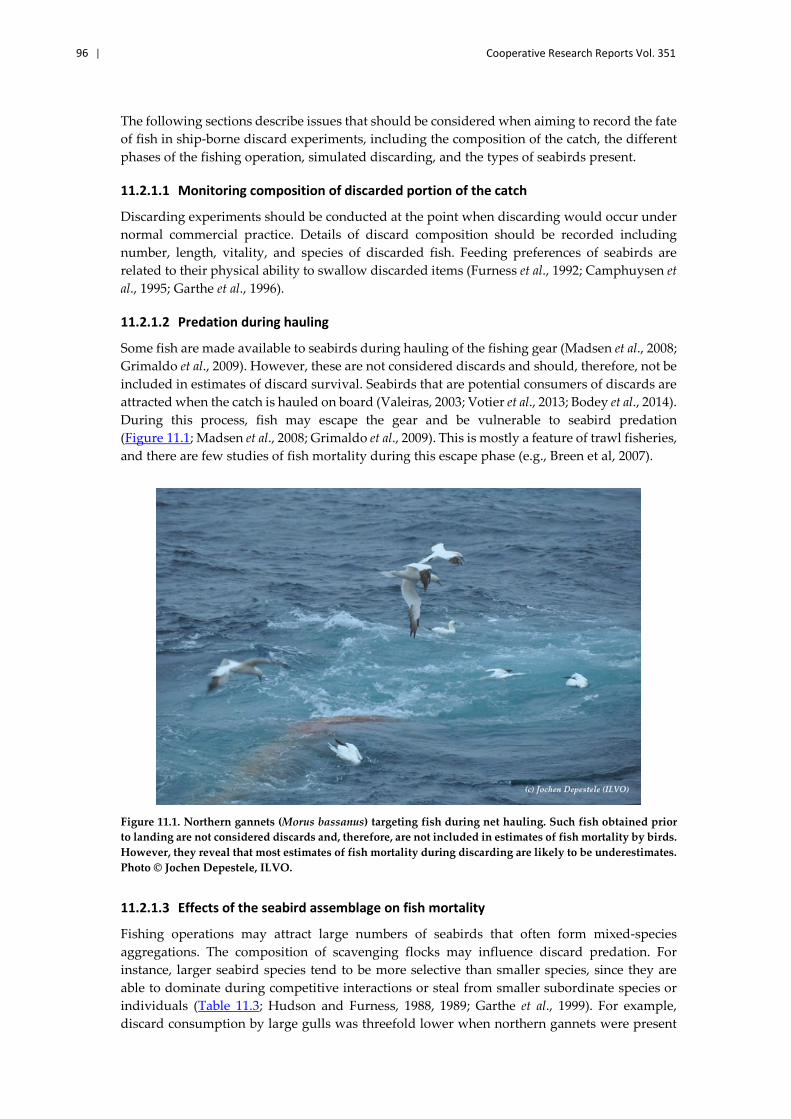
96 | Cooperative Research Reports Vol. 351
The following sections describe issues that should be considered when aiming to record the fate of fish in ship-borne discard experiments, including the composition of the catch, the different phases of the fishing operation, simulated discarding, and the types of seabirds present.
11.2.1.1 Monitoring composition of discarded portion of the catch
Discarding experiments should be conducted at the point when discarding would occur under normal commercial practice. Details of discard composition should be recorded including number, length, vitality, and species of discarded fish. Feeding preferences of seabirds are related to their physical ability to swallow discarded items (Furness et al., 1992; Camphuysen et al., 1995; Garthe et al., 1996).
11.2.1.2 Predation during hauling
Some fish are made available to seabirds during hauling of the fishing gear (Madsen et al., 2008; Grimaldo et al., 2009). However, these are not considered discards and should, therefore, not be included in estimates of discard survival. Seabirds that are potential consumers of discards are attracted when the catch is hauled on board (Valeiras, 2003; Votier et al., 2013; Bodey et al., 2014). During this process, fish may escape the gear and be vulnerable to seabird predation (Figure 11.1; Madsen et al., 2008; Grimaldo et al., 2009). This is mostly a feature of trawl fisheries, and there are few studies of fish mortality during this escape phase (e.g., Breen et al, 2007).
Figure 11.1. Northern gannets (Morus bassanus) targeting fish during net hauling. Such fish obtained prior to landing are not considered discards and, therefore, are not included in estimates of fish mortality by birds. However, they reveal that most estimates of fish mortality during discarding are likely to be underestimates. Photo © Jochen Depestele, ILVO.
11.2.1.3 Effects of the seabird assemblage on fish mortality
Fishing operations may attract large numbers of seabirds that often form mixed-species aggregations. The composition of scavenging flocks may influence discard predation. For instance, larger seabird species tend to be more selective than smaller species, since they are able to dominate during competitive interactions or steal from smaller subordinate species or individuals (Table 11.3; Hudson and Furness, 1988, 1989; Garthe et al., 1999). For example, discard consumption by large gulls was threefold lower when northern gannets were present

ICES Guidelines on Methods for Estimating Discard Survival | 97
in the flock of ship-following seabirds (Depestele et al., 2016). As another example, gannets have a preference for larger roundfish (Garthe and Hüppop, 1998); therefore, the risk of predation on discarded roundfish increases with larger numbers of gannets. The presence of seabirds that steal prey from conspecifics or heterospecifics via kleptoparasitism (e.g. skuas and gulls) will also have both direct and indirect influence on discard consumption (Garthe and Hüppop, 1998). Moreover, species with greater diving abilities may be able to capture fish as they sink through the water column (e.g. gannets and shearwaters), which is not the case for surface gleaners (e.g. gulls).
Table 11.3. Foraging success index (experimentally discarded fish swallowed on average per bird of each species present over all fishing trips) for different seabirds feeding on fish discarded from trawling fishing boats in Shetland during the summers of 1984 and1985 (Furness et al., 1992). These results reveal that larger species have a higher success index, highlighting the importance of quantifying the composition of the scavenging seabird assemblage.
Species Mean number at boat
Total number of fish swallowed Success index
Gannet 9 452 50
Great skua 12 347 29
Great black-backed gull 234 2 753 12
Lesser black-backed gull 6 32 5.3
Herring gull 30 107 3.6
Fulmar 485 85 0.2
Kittiwake 3 0 0
11.2.1.4 Effects of the availability of alternative seabird food on fish mortality
While many seabirds have become specialized discard consumers (Votier et al., 2010; Patrick et al., 2015), the predation rates of discarded fish may vary as a function of their availability or the season of the year (Votier et al., 2004, 2008). For example, non-breeding gannets feed extensively on fishery waste, but they will double their diving efforts to provide their chicks with higher quality, live pelagic fish (Grémillet et al., 2008).
11.2.1.5 Discharge rates and methodology
The most common general approach to seabird discard predation assessments is the manual selection of fish, that are then discarded by observers and their fate recorded. However, specific methodologies of discard experiments can vary, and may have profound consequences for estimating fish morality rates.
The discarded items are either returned to the sea during single-item simulated discard experiments (Camphuysen et al., 1995; Walter and Becker, 1997; Sotillo et al., 2014) or during multi-item experiments (Arcos et al., 2001; Catchpole et al., 2006; Gonzalez-Zevallos and Yorio, 2011; Jodice et al., 2011). The advantage of single-item discard experiments is the ability to accurately determine the fate of each item, but a disadvantage is that this can be unrepresentative of normal commercial practices.
It is not known whether different simulated discard patterns significantly alter fish mortality estimates. One study found no clear difference in fish predation by seabirds between single- and multi-item discard experiments (Garthe et al., 1998). In contrast, another found that the

98 | Cooperative Research Reports Vol. 351
consumption by birds of discarded compressiforme fish was lower when 50 fish were discarded at once, than when fish were discarded at a rate of 2.4 fish per s (Figure 11.2; Depestele et al., 2016). Best practice should favour experiments with realistic discarding rates, which simulate commercial practice as far as possible.
Knowing the vitality of the fish that are being discarded is the key element to for quantifying the effect of seabird predation on the survival of discarded fish. It is essential to apply the same vitality assessments to the fish subject to discard simulations, as those used for other parts of the study (tagging, captive observation). Only with this information is it possible to apply seabird predation survival rates to the health profile of the discarded catch. At present, tagging is more suited to larger fish (skates, rays, large gadoids) which are unlikely to be affected by seabird predation, owing to the limits of miniaturization of the technology. Captive observation studies are applied to smaller fish, but these studies do not include estimates of predation. However, quantified seabird predation estimates by vitality category (and other factors e.g. size) can be used to adjust captive observation estimates to include seabird predation levels.
0.0%
10.0%
20.0%
30.0%
40.0%
50.0%
60.0%
70.0%
boarfish roundfish
Experimental Discard Consumption by northern Gannets in the Bay of Biscay
all at once 2.4 items per second
Figure 11.2. Experimental discard consumption by northern gannets in the Bay of Biscay. These data reveal that the rate of discarding influences fish mortality for some fish (roundfish), but not for others (boarfish). Therefore, in some cases, fish mortality estimates based on slow rates of discarding will not be reliable. Roundfish species include Argentina spp, Melanogrammus aeglefinus, Merluccius merluccius, Micromesistius poutassou, Scomber scombrus, Trachurus trachurus, Trisopterus spp, Sebastes spp. (Depestele et al., 2015, © Ghent University, Belgium).
11.2.1.6 Selection of fish for simulated discarding
The selection of fish for discard simulations will greatly influence the seabird predation levels observed. As mentioned, feeding preferences of seabirds are related to their ability to swallow discarded items.
11.2.1.7 Effect of discarding practices
Different gear types, fishing operations, and behaviour of fishers will lead to variation in the manner of discarding practices, with consequences for fish predation by seabirds. Discard consumption may be affected by the location of discarding, vessel movements and the turbulence generated by the engines (Hudson and Furness, 1988). Therefore, there may be

ICES Guidelines on Methods for Estimating Discard Survival | 99
different levels of avian predation even within fishing métiers that have comparable vessels and discarding practices. As a consequence, reliable estimates of fish mortality are likely to only be available for specific fisheries. Confidence in extrapolating estimates of seabird predation will require information on the range of vessel operations, including deck layout and sorting practices, and the catch composition. These potentially confounding factors indicate that fish mortality estimates may be highly specific to location, métier, vessel, and date. Conducting targeted experiments to better understand how to control for this wide variety of factors would be advantageous.
11.3 Analysis of avian predation data and estimating survival
Seabird predation represents the first life-threatening challenge that discarded fish face immediately post-release. As such, it has the potential to be a significant modifier of the survival rates obtained from captive observation and tagging methods, both of which are likely to implicitly exclude avian predation from their studies effects. Captive observation typically gives the test subject protection from most forms of predation (Section 9). Tagging can be informative about post-release predation once the subject has left the surface, but it would be a wasteful use of resources to allow tagged fish to be taken by seabirds as they are released back to the sea (Section 10).
To account for avian predation in an integrated estimate of post-release survival (Section 13.6), the minimum information required about avian predation is the likelihood of escape. This information is available from discard consumption studies, which provide categorical data on the fates of individual fish (Table 11.4). It is possible to make clear inferences from some of these observed fates that the fish did not escape, particularly if the fish (or its viscera) is eaten and not regurgitated. However, with regard to successful escapes, there is some degree of uncertainty in most cases. Even where fish are observed to have actively swum away, there will be some doubt as to whether it was caught out of sight by a diving bird. Furthermore, it is likely that a fish which directly encountered a seabird but successfully escaped, may have its vitality and, likely, its survival compromised due to injuries and/or stress; thus potentially biasing assumed post-release survival rates. However, at the very least, it will be possible to provide a “best case” minimum estimate for the proportion of the population that did not escape.
Table 11.4. Inferences relating to avian predation on discard fish that can be made from vessel-based observations (see 11.2.1).
Fate recorded by observer Inference about escape status
Picked up and swallowed Dead, unless regurgitated
Picked up and stolen by another species Dead, unless regurgitated
Viscera consumed, fish left in water Dead
Picked up and dropped Unknown, vitality status may have been modified
Ignored; lost to view on surface with unknown fate Unknown, fate likely linked to vitality status
Fish sank out of view Possible escape, depending on vitality status
Fish observed actively swimming from view Probable escape, depending on vitality status
The escape likelihood data should be provided in context with significant explanatory variables that are relevant to survival, e.g. species, size, and vitality. To this end, it would be informative

100 | Cooperative Research Reports Vol. 351
to model predation-fate data with respect to these and other important explanatory variables, e.g. fish shape, discarding practices, composition of the scavenging flock. As these predation-fate data are ordinarily categorical, an appropriate approach would be to fit using the proportional-odds multinomial linear model described in Section 13.3.1.
11.4 Summary
A wide variety of species may be important as consumers of discards, and they may be eating discards as predators and as scavengers, i.e. consuming already dead discards. Seabird predation is specifically included here because (i) seabirds forage at or near the sea surface, are one of the first predatory threats to discards, and can be visually observed with relative ease; (ii) they are the most abundant discard scavengers in some fisheries, and (iii) other approaches to estimating discard survival do not account for avian predation.
Current estimates of seabird predation do not discriminate between discards that are already dead and others that may survive. The methods, therefore, require revisiting to explicitly assess seabird predation of discarded fish in relation to the influence on discard survival. A two-tier approach is proposed to (i) estimate the risk of seabird predation in a fishery and (ii) make direct observations of discard predation mortality from ship-based research.
The risk of seabird predation in a fishery is determined by (i) the association of seabirds with a fishery and (ii) the dietary preferences of the seabirds. When a high number of seabirds are associated with a fishery and discard species are favourable food items, seabird predation may influence discard survival. The distribution of scavenging seabirds can be established by boat-based and aerial surveys, land-based studies, biologging, and autonomous vehicles, while data on the distribution of fisheries is collected as part of fisheries management.
The dietary preferences of seabirds can be determined from methods using stable isotopes and fatty acids, biologging, or conventional dietary assessment tools. In cases where seabird and fishery distributions overlap and dietary preferences are relevant to the discard composition, ship-based research should be applied to estimate whether seabird predation is on dead discards or live discards and if it is influenced by the health (vitality) of the fish (sections 8, 9, and 10).
On-board observers can record the fate of discarded fish. This will be (i) picked up and dropped; (ii) picked up and swallowed; (iii) picked up and stolen by another species; (iv) ignored; (v) lost from view at the surface with unknown fate; (vi) sank out of view; or (vii) observed actively swimming out of view. To estimate discard mortality by seabird predation, an assessment of the vitality of discarded individuals (Section 8) must be coupled to estimates on the fate of the discards. This is due to the likelihood that seabirds will preferentially predate on the least vital discards. Similarly, the assemblage of seabirds should be recorded as predation success will also be influenced by interspecies competition for discards.
Simulated discard experiments should try to replicate normal discarding practice as far as possible, i.e. the composition of discards and how the discards are jettisoned from the vessel, since this may affect avian predation on the discard. For example, single-discard-item tracking can be achieved more easily by an observer, but may not generate representative levels of predation if normal discarding is of multiple items simultaneously. Details on all of these aspects of avian predation assessments have been provided in this section.

ICES Guidelines on Methods for Estimating Discard Survival | 101
12 Survival data: format, structure, and simple summary analysis
Mike Breen and Hugues Benoît
Survival assessments produce data in a range of different formats that can be used to answer several objectives (see sections 3 and 4), including:
• providing a simple estimate (with a confidence interval) of the discard survival potential of a species;
• demonstrating a species has a discard survival potential significantly above a specified threshold (e.g. for the “High Survival” exemption to the EU Landing Obligation; Rihan et al, 2019);
• comparing the effectiveness of different mitigation measures for improving discard survival; and/or
• investigating the likely causes of discard mortality by modelling survival data with explanatory variables.
To address these objectives, sections 12 and 13 provide an introduction to survival data and their analysis:
• Section 12 introduces the reader to survival data, the different forms they take, their properties, and important considerations for data summary and presentation. It is recognized that many of the readers of the guidance notes may have limited knowledge of statistical techniques. To accommodate this, Section 12 has been written as “user-friendly” introduction. Consequently, the methods and examples it presents are relatively simple and may only have limited application in the more complex experimental designs seen in many real survival assessments. Nonetheless, these “simple” techniques, as well as the form and properties of survival data, are important to understand when using more advanced techniques (as described in Section 13).
• Section 13 provides a more in-depth overview of the statistical modelling techniques used to investigate the influence of potential explanatory variables on survival. The text in section 13 is intended for readers with a more advanced statistical knowledge. However, it will hopefully also provide less-experienced users with a useful insight into these statistical techniques, along with references to additional detailed resources to learn more about them.
• In addition, Section 5 - Experimental Design - draws on information from both sections 12 and 13 to provide examples of sound approaches to good experimental design.
These sections all provide worked examples, many of which use the statistical computing and programming language R (R Core Team, 2017). The “R” software and supporting packages are free and are continuously developed and updated by a large and supportive online community. Code for these examples is provided in the text, as well as in the Online Support Materials (OSM2). In addition, all mathematical notation is summarised and defined in Annex 1.
In drafting these sections, the aim was not to write a statistical textbook, but to provide the reader with a useful starting reference to sources of information on the most appropriate analytical methods for their data. It is recommended that at all stages of the analysis process,
2 https://github.com/ices-publications/CRR351-OSM

102 | Cooperative Research Reports Vol. 351
including the initial experimental design, users of this manual should consult with a statistician for further and more specific guidance.
12.1 Survival data: types and properties The main objective of survival assessments is to describe the proportion of the population that can survive capture and release from fishing gear. For every subject (e.g. fish) being monitored in a sample from a population, there are two possible outcomes when an observation is made: they may either be “dead” or “alive”. This type of data is called “binary”, “binomial”, or “dichotomous” data.
Depending on how survival is being described with respect to time, data can take one of two forms: “cross-sectional” and “longitudinal”. Cross-sectional data describes the proportion of surviving animals at one or more specific points in time. At their most basic, longitudinal data comprise mortality times for individual fish. Longitudinal data are used to estimate a survivorship function that effectively describes the proportion of surviving animals as a continuous function of time. Further details on each type of data are given in the following subsections.
12.2 Cross-sectional data
The true proportion of surviving (p) and dying (q) animals in a population of animals released from fishing gear are the “measures of interest” in survival assessments. However, they can be difficult to determine in absolute terms because it is simply not possible to observe every fish released from fishing gear. Instead estimates of survival (p) and mortality (q) can be generated from representative samples of the released population (Section 5.1).
Binomial data can be defined as the result of an event (e.g. the survival of a discarded fish) that can be summarized by one of two outcomes: success or failure, or, in this case, alive or dead. For a sample taken from a population, the number of subjects still alive (s) or dead (r) at any point in time (t) can be used to define an estimator of the survival probability (p) or mortality probability (q):
��𝑝𝑡𝑡 = 𝑠𝑠𝑡𝑡𝑛𝑛𝑡𝑡
𝑞𝑞�𝑡𝑡 = 𝑟𝑟𝑡𝑡𝑛𝑛𝑡𝑡
(2)
where p = 1 – q and n = s + r.
This form of summary statistic is very common in survival studies. It will be familiar to many readers as estimators of probabilities (0 ≤ p ≤ 1), which can also be expressed as percentages. It is important to remember that these statistics refer to observations at a specific point in time (t), typically the end of the monitoring period.
As discussed in Section 2.3, mortality associated with the stress of being caught and released from a fishing gear is not instantaneous. Therefore, to accurately reflect overall mortality resulting from that stress, the final observation should be made at a point in time when the resultant mortality has ended, or when the survival curve has reached its asymptote, i.e. the asymptotic survival estimate (SA; Information Box 12.1). This emphasizes the importance of monitoring survival repeatedly over a period of time (i.e. longitudinal data). However, a single point observation (i.e. cross-sectional data) can still be valuable, ideally as long as it is collected once SA has been reached, or a suitable correction can be made to account for the difference between the estimate and SA. In reality, many survival assessments do not achieve this ideal, so the following text will simply refer generally to “survival estimates”, unless specified otherwise.

ICES Guidelines on Methods for Estimating Discard Survival | 103
This section will continue by exploring the properties of cross-sectional binomial data and the binomial distribution, and how these can be used to define a meaningful measure of uncertainty in the data, the confidence interval.
Information Box 12.1. Asymptotic survival (SA)
The observed survival at asymptote or “asymptotic survival” (SA) defines an observable endpoint where it is assumed that all study subject mortality associated with the treatments has already occurred. As such, it is an important concept in survival assessments.
Any experiment that is terminated before asymptotic survival has been observed or inferred will likely lead to an overestimation of discard survival, unless an appropriate correction can be made. For example, Figure 12.1 illustrates that a cross-sectional mortality estimate taken at time-point 1 (t1) would overestimate SA, whereas an estimate taken at a second time point (t2) would not. This helps define how long experimental subjects should be observed in an assessment to ensure that the overall discard survival is not overestimated.
Figure 12.1. An example of survival probability over time (longitudinal survival data) illustrating asymptotic survival (SA). A cross-sectional estimate of survival taken at time point 1 (t1) would over-estimate SA, whereas an estimate taken at time point 2 (t2) would accurately reflect the SA.
SA can be defined mathematically (from the shape of the survival curve or function). Consequently, where assessments have knowingly not been able to monitor to the asymptote, SA may still be estimated, along with the associated uncertainty, by applying a suitable mathematical model (Section 13.2).
A valid SA estimate may not be attainable in all cases. For example, a treatment can induce chronic fatal mechanisms that kill affected subjects over a prolonged period of time. In this case, estimated discard survival would be zero. Finally, it should be noted that it is unrealistic to assume that mortality will end completely, as there will always be an underlying natural mortality in any population (Section 6). However, over the time-scales that most survival assessments are conducted, it is likely that any underlying natural mortality will be indistinguishable from zero.

104 | Cooperative Research Reports Vol. 351
12.2.1 The binomial distribution
The likelihood of survival events in a population can be modelled using a discrete probability distribution: the binomial distribution. This describes the probability of observing a particular number of survivors in a sample (s), given that you know the probability of an individual surviving (p) and the size of the sample (n):
Pr(𝑋𝑋 = 𝑠𝑠) = �𝑛𝑛𝑠𝑠� 𝑝𝑝𝑠𝑠(1 − 𝑝𝑝)𝑛𝑛−𝑠𝑠 (3)
For s = 0, 1, 2, … , n, where:
�𝑛𝑛𝑠𝑠� = 𝑛𝑛!𝑠𝑠!(𝑛𝑛−𝑠𝑠)!
; the binomial coefficient. (4)
Figure 12.2 shows the distribution of probabilities for a sample size (n) of 20, where p = 0.5. Here, it can be seen that the most likely number of survivors would be 10. However, it can also be seen that it is possible to have observations with either larger or smaller numbers of survivors, but these decrease in likelihood the farther we deviate from 10.
Figure 12.2. An example of a binomial discrete probability distribution (grey bars) where n = 20 and p = 0.5. When n is large and p is ca. 0.5, the binomial distribution approximates the normal distribution (blue line). Mean = n.p. Variance = n.p.q = n.p. (1–p).
For any binomial distribution, the mean and variance can be estimated as simple functions of n and p (Figure 12.2). Furthermore, the standard error for the estimator p (equation 2) can be estimated as ���𝑝(1 − ��𝑝) 𝐵𝐵⁄ . A closer examination of these estimators reveals that binomial data have some important properties preventing the use of methods that have been developed for normally distributed data:
• The estimator for the mean is bounded (i.e. 0 ≤ p ≤1). That is, for binomial data, no value of p can be < 0 or > 1. Conversely, normally distributed data can take any value between ₋∞ (minus infinity) and ∞ (infinity). This becomes important when trying to model binomial data. A simple linear model (i.e. a straight line) should not be used to describe the relationship between the observed survival and any explanatory variables. Such a linear model could start predicting impossible survival estimates (i.e. < 0 and > 1). This issue can be addressed by (i) transforming the data (e.g. arcsin),

ICES Guidelines on Methods for Estimating Discard Survival | 105
which is an ad hoc approach, or (ii) by using models that are adapted for binomial responses, which is the preferred approach (i.e. 0 ≤ p ≤ 1; Section 13.1).
• The variance and standard error are not constant. For binomial data, variance and standard error are a function of, and, therefore, vary with, different values of p and n. Figure 12.3 shows that the standard error is highest when p is 0.5, and decreases as p approaches 0 or 1. This relative change in standard error is scaled by the sample size (n), and is smaller as n increases (Figure 12.3).
• The distribution is generally not symmetrical. Figure 12.4 shows that when p is close to 0.5, and n is large (≥ 25) the distribution of the number of survivors is approximately bell-shaped and symmetrical. However, as p approaches 0 or 1 the distributed becomes limited by the boundary values and becomes asymmetrical. This again has important implications when modelling binomial data, in particular with respect to how the residuals are distributed around the fitted values in a model. Interestingly, when p is close to 0.5 and/or n is large, the binomial distribution approximates the Normal (Gaussian) distribution, which has been used to simplify analysis of binomial data by using normal approximations, for example the Wald’s statistic (Newcombe, 2013).
Figure 12.3. The standard error (s.e.) of the estimated probability of survival (p) is estimated as �𝒑𝒑�(𝟏𝟏 − 𝒑𝒑�) 𝒏𝒏⁄ and varies with p, where s.e. is greatest when p = 0.5. Increasing sample size (n) reduces the scale of this effect across the range of p.
12.2.2 Confidence Intervals: a measure of uncertainty.
Survival assessments aim to produce an overall estimate of discard survival for a population based on measurements from a representative sample of the population. However, how precisely does this sample estimate reflect the “true” (unknown) survival probability for the wider population in general? Confidence intervals (CI) provide information on the uncertainty around an estimated parameter from a sample, and are fundamental elements in hypothesis testing (Section 12.2.2.4), interpreting survival (binomial) results (Section 12.4) and making inferences from models of observed data (Section 13). The CI gives a range of values for the estimated parameter (e.g. sample mean, ��𝑥), with some level of “confidence” on how accurately it reflects the true population parameter (e.g. population mean, X). The confidence level is typically expressed as a percentage (e.g. 95%) and, as a frequentist concept, should be interpreted as the percentage of times that the true population parameter (e.g. population mean,

106 | Cooperative Research Reports Vol. 351
X) would lie within the CI around the sample estimate (e.g. sample mean, ��𝑥), if the sampling was repeated in the same way a large number of times. This is often misinterpreted as meaning there is a 95% probability that the true population survival will be within the sample’s confidence interval. However, for any one CI, the true value either is or is not contained in the interval and, therefore, the interval cannot contain the true value with some probability (Trkulja & Hrabač, 2019). Thus, it follows that sampling theory states that multiple observations (i.e. large sample sizes and numbers of replicates) are important for obtaining accurate and precise parameter estimates. Though it is not expanded upon here, the Bayesian paradigm includes the “credibility interval” (Crl) which is interpreted as having some probability of containing the true value, in contrast to the confidence interval above (Newcombe, 2013).
Figure 12.4. Binomial probability mass functions for increasing sample size (n = 5, 25, or 125) and for two probability values (p = 0.5 or 0.8). Note that the distribution is always skewed unless p = 0.5, but it approximates a normal distribution as n increases.
For binomial proportions, the simplest forms of CI are those where the data distribution can be approximated to a normal distribution, and, thus, the corresponding theory can be applied (Hazewinkel, 2001; Crawley, 2013; Section 12.2.2.1). However, because the binomial distribution only approximates the normal distribution under specific circumstances, alternative methods are required for the general application of binomial confidence intervals (Section 12.2.2.2).
The following subsections will describe how a confidence interval can be estimated with respect to normally distributed data, and explain the fundamentals of the approach (Section 12.2.2.1). Building on this, Section 12.2.2.2 explains the calculation of the normal approximation for the Binomial CI . Finally, alternative methods for estimating binomial CIs will are introduced in sections 12.2.2.3 and12.2.2.4. Worked examples are provided throughout.
12.2.2.1 Confidence intervals and their application to normally distributed data
Key characteristics of the normal distribution are:
i) values are symmetrically distributed on either side of the mean (to ± ∞); and
ii) the majority of values are centred close to the mean (ca. 95% within 1.96 standard deviations (s.d.) of the mean, ca. 90% within 1.645 s.d., and ca. 99% within 2.57 s.d.).
Figure 12.5 shows the probability density distribution for a normal distribution (with mean = 0 and standard deviation = 1). The area under this curve represents the probability of finding a value in a normally distributed population that differs from the mean by a certain amount; in

ICES Guidelines on Methods for Estimating Discard Survival | 107
this example, measured in standard deviations. By assuming that this distribution represents the very large number of samples imagined in the frequentist sampling theory (described above), it is possible to define a threshold on the x-axis (a quantile) that partitions a desired proportion of the distribution equal to the required confidence level (e.g. 95%). This can be simply done using a “standard normal or Z-table”. Conveniently, it can also be done using the R function qnorm.
That is, using the one-tailed quantile (Z1 – α) for a particular confidence level (1 – α; where α = significance level; see Section 5.3) and the standard error of the estimate (s.e.), a “one-sided confidence interval” (CI) can be defined with respect to the population mean (i.e. the sample mean, ��𝑥):
𝐶𝐶𝑁𝑁𝐵𝐵𝑜𝑜𝑖𝑖𝑜𝑜𝑡𝑡𝐵𝐵𝑜𝑜𝑡𝑡 𝑖𝑖𝐵𝐵𝑡𝑡𝑡𝑡𝑡𝑡𝑖𝑖𝑡𝑡𝑖𝑖 (𝑁𝑁𝐵𝐵𝑡𝑡 𝑠𝑠𝑖𝑖𝑜𝑜𝑡𝑡𝑜𝑜, 𝑖𝑖𝑁𝑁𝑙𝑙𝑡𝑡𝑡𝑡)(1 − 𝛼𝛼): ��𝑥 − 𝑍𝑍1−𝛼𝛼 ∙ 𝑠𝑠𝑡𝑡 ↔ +∞ (5)
𝐶𝐶𝑁𝑁𝐵𝐵𝑜𝑜𝑖𝑖𝑜𝑜𝑡𝑡𝐵𝐵𝑜𝑜𝑡𝑡 𝑖𝑖𝐵𝐵𝑡𝑡𝑡𝑡𝑡𝑡𝑖𝑖𝑡𝑡𝑖𝑖 (𝑁𝑁𝐵𝐵𝑡𝑡 𝑠𝑠𝑖𝑖𝑜𝑜𝑡𝑡𝑜𝑜,𝑢𝑢𝑝𝑝𝑝𝑝𝑡𝑡𝑡𝑡)(1 − 𝛼𝛼) : − ∞ ↔ ��𝑥 + 𝑍𝑍1−𝛼𝛼 ∙ 𝑠𝑠𝑡𝑡 (6)
For 90% confidence, Z1 – α = 1.28
For 95% confidence, Z1 – α = 1.64
For 99% confidence, Z1 – α = 2.33
For example, -qnorm(1–0.05) gives a one-sided lower quantile (Z1 – α) value of –1.64, where there is a 5% probability of finding a lower value, and a 95% probability of finding a higher value (Figure 12.5 a). By applying these to equation 5, for a sample mean of 1.86, with a s.e. of 0.2, the one-sided lower 95% confidence interval is estimated to be: 1.86 – (1.64 ∙ 0.2) = 1.532.
Alternatively, by defining outer tails of the distribution above and below which 2.5% (i.e. 5%/2) of the values lie [± qnorm(1-0.025)], it is possible to define the thresholds within which 95% of the values lie symmetrically about the mean. A “confidence interval” (CI) can be then defined around an estimate of the population mean (i.e. the sample mean, ��𝑥) using the standard error of the estimate (s.e.) and the appropriate two-sided normal quantiles (Z1 – α/2) for a particular confidence level (1 – α):
𝐶𝐶𝑁𝑁𝐵𝐵𝑜𝑜𝑖𝑖𝑜𝑜𝑡𝑡𝐵𝐵𝑜𝑜𝑡𝑡 𝑖𝑖𝐵𝐵𝑡𝑡𝑡𝑡𝑡𝑡𝑖𝑖𝑡𝑡𝑖𝑖 (𝑡𝑡𝑙𝑙𝑁𝑁 𝑠𝑠𝑖𝑖𝑜𝑜𝑡𝑡𝑜𝑜) (1 − 𝛼𝛼): ��𝑥 ± 𝑍𝑍1−𝛼𝛼/2 ∙ 𝑠𝑠𝑡𝑡 (7)
For 90% confidence, Z1 – α/2 = 1.64
For 95% confidence, Z1 – α/2 = 1.96
For 99% confidence, Z1 – α/2 = 2.57
Applying the example values above (mean 1.86 and s.e. 0.2) and Z1 – α/2 = 1.96 to equation 7, the two-sided lower 95% confidence interval is estimated to be: 1.86 ± (1.96 ∙ 0.2) = 1.468 to 2.252. Alternatively, if a higher level of confidence was required (e.g. 99%), the outer tails of the distribution above and below which 0.5% (i.e. 1%/2) of the values lie [± qnorm(1-0.005)] gives Z1 – α/2 = 2.57. Applying to equation 7, the two-sided lower 99% confidence interval is estimated to be: 1.86 ± (2.57 ∙ 0.2) = 1.346 to 2.374.
From these examples, it is clear that the width of the interval increases for greater levels of confidence (1 – α), because a greater range of values must be included to ensure greater confidence. Likewise, the CI for a given confidence level will be wider, with increasing standard error in the sample, because there is less certainty in the accuracy of the estimate.

108 | Cooperative Research Reports Vol. 351
a)
b)
Figure 12.5. Normal probability density distribution, Norm(mean = 0, s.d. = 1), showing a) one-sided and b) two-sided 95% quantiles.
12.2.2.2 Binomial Confidence intervals
From equation 4, it follows that it is possible to define a synonymous confidence interval for the estimated survival probability (p, equation 2) in the binomial distribution. This is commonly known as the Wald interval or normal approximation of the binomial CI (Newcombe, 2013):
��𝑝 ± 𝑍𝑍1−𝛼𝛼/2 ∙ �𝑝𝑝�(1−𝑝𝑝�)
𝑛𝑛 (8)
However, as discussed in Section 12.2.1, the binomial distribution only approximates the normal distribution in limited circumstances (i.e. when n is large and/or p is ca. 0.5). Furthermore, because the binomial distribution is discrete and the probability p is bounded (by 0 and 1), as opposed to the normal distribution (which is continuous and has support over positive and negative infinity), this approach generally produces inadequate confidence intervals, particularly when n.p <10 and n(1 –p)<10 (Newcombe, 2013, p. 56).
Defining appropriate confidence intervals for the binomial distribution when the normal approximation is not applicable, has been a considerable challenge in statistics (Newcombe,

ICES Guidelines on Methods for Estimating Discard Survival | 109
2013). Numerous alternative methods to the Wald interval have been published, including the “adjusted Wald” or Agresti-Coull intervals (Agresti and Coull, 1998), Clopper-Pearson “exact” method (Clopper and Pearson, 1934), and Wilson score method (Wilson, 1927). However, no ideal solution to suit all circumstances has yet been identified. Several reviews have been conducted of the different methods, including “exact” methods, and the general consensus is that the Wilson score method is the most reliable, closed-form method (i.e. can be calculated analytically; Brown et al., 2001, 2002; Pires and Amado, 2008; Newcombe, 2013; Wallis, 2013):
𝑊𝑊𝑖𝑖𝑖𝑖𝑠𝑠𝑁𝑁𝐵𝐵 𝑠𝑠𝑜𝑜𝑁𝑁𝑡𝑡𝑡𝑡 𝑖𝑖𝐵𝐵𝑡𝑡𝑡𝑡𝑡𝑡𝑖𝑖𝑡𝑡𝑖𝑖 (𝑙𝑙−,𝑙𝑙+) = ���𝑝 + 𝑍𝑍2
2𝑛𝑛 ± 𝑍𝑍 ∙ �𝑝𝑝�(1−𝑝𝑝�)
𝑛𝑛+ 𝑍𝑍2
4𝑛𝑛2� �1 + 𝑍𝑍2
𝑛𝑛�� (9)
Bayesian or Beta intervals offer reliable alternatives to the frequentist methods discussed above, with several favourable properties. However, they require more advanced techniques to calculate them (Newcombe, 2013). For the purposes of this report, and the practical application of binomial confidence intervals when reporting the results of survival assessments, the frequentist methods are considered perfectly adequate.
12.2.2.3 Resources for calculating binomial confidence Intervals
The R package “Binom” (2014) has several useful functions for defining and assessing the reliability of binomial confidence intervals, i.e. interval width, coverage, and statistical power (see Newcombe, 2013 for information on assessing the properties of confidence intervals). The function “binom.confint” provides estimates of binomial confidence intervals with the option of using a variety of methods, including the Wilson score, the Wald, the Agresti-Coull and the Clopper-Pearson “exact” methods (Table 12.1).
Table 12.1. Estimated binomial confidence intervals for the proportion 0.7 (70/100) using eleven different methods on the R function “binom.confint” [in “Binom”]. [where, s = number of successes or “survivors”; n = total number in trial or “sample”; p = estimated proportion or “survival”]. Note: because of the conditional nature of Bayesian methods, estimates of p can vary slightly from simple proportions.
Method s n p Lower Upper
Agresti-Coull 70 100 0.700 0.604 0.781
asymptotic 70 100 0.700 0.610 0.790
Bayes 70 100 0.698 0.608 0.786
cloglog 70 100 0.700 0.600 0.780
exact 70 100 0.700 0.600 0.788
logit 70 100 0.700 0.603 0.782
probit 70 100 0.700 0.605 0.783
profile 70 100 0.700 0.606 0.784
lrt 70 100 0.700 0.606 0.784
prop.test 70 100 0.700 0.599 0.785
Wilson 70 100 0.700 0.604 0.781

110 | Cooperative Research Reports Vol. 351
12.2.2.4 Confidence intervals and hypothesis testing
Users of the data from survival assessments may ask the question, “Is the observed survival significantly greater than H?”, where “H” is a threshold defining “high survival”. In this case, the researcher may conduct a hypothesis test based on a one-sided CI, to establish whether there is a significant difference between the estimated survival and the threshold value.
For example, using the R function “binom.test”, the user can assess whether an estimated survival rate (e.g. based on 65 survivors out of a total of 100) is significantly greater than a nominal “high survival” threshold of 60%. (Note: this function is from the “stats” package which by default uses the Clopper-Pearson “exact” method to define CIs, which tends to be more conservative than the “Wilson score” method because it estimates slightly wider intervals; Table 12.1).
> binom.test(65, 100, p=0.6, alternative = "greater")
Exact binomial test
data: 65 and 100
number of successes = 65, number of trials = 100, p-value = 0.1795
alternative hypothesis: true probability of success is greater than 0.6
95 percent confidence interval: 0.5639164 1.0000000
sample estimates: probability of success 0.65
In this example, although the sample proportion estimate (i.e. 0.65) is greater than the threshold value (0.60), the confidence interval contains the threshold value and, hence, the result is not significant (p = 0.1795). In contrast, if the sample size had been larger (e.g. 650/1000 survivors), the same proportion would be produced (0.65), but the CI would not contain the threshold value. In this case, the result is significant at the 5% level (i.e. p < 0.05).
> binom.test(650, 1000, p=0.6, alternative = "greater")
Exact binomial test
data: 650 and 1000
number of successes = 650, number of trials = 1000, p-value = 0.0006455
alternative hypothesis: true probability of success is greater than 0.6
95 percent confidence interval: 0.624385 1.000000
sample estimates: probability of success 0.65
Summary - Binomial CIs
In summary, CIs are important tools for interpreting survival (binomial) results (Section 12.4) and making inferences from models of observed data (Section 13). The principles and the application of these tools are well established for normally distributed data, and data that approximates a normal distribution. Establishing reliable confidence intervals for binomial data has been an ongoing challenge for statistical science, leading to an array of alternative methods for estimating the confidence interval around a proportion. This section recommends the use of the “Wilson Score” method, based on a consensus from the scientific literature.

ICES Guidelines on Methods for Estimating Discard Survival | 111
12.3 Longitudinal data
Event times (longitudinal data) constitute the data format that is naturally recorded during survival assessments when there is an ongoing/repeated monitoring of experimental subjects. This format consists of a list of times within the observation period when different individuals were observed to have died, along with the number of survivors at the end of the observation period. These data can be expressed as a “life table”, which shows the cumulative total of animals that are dead and alive at each observation time point. Building on the previous sections, these data in the “life table” can be used as estimates of the proportion of surviving animals at different points in time, with the appropriate CI.
Furthermore, this simple “life table” approach can be used to produce an estimate of asymptotic survival (SA; namely, the final survival estimate in the time-series), provided that the post-treatment monitoring period was sufficiently long and mortality in the sample had ceased (Information Box 12.1). However, this “life table” approach does not fully utilize the added dimension of time within the data, or, more specifically, the rate at which the animals are dying, to better understand the observed mortality. As discussed in Section 2, the rate at which animals die can be very informative about the underlying causes of mortality; and where these data exist, they should be utilized.
It can be seen intuitively, and written mathematically, that cross-sectional data are merely a special case of longitudinal data, i.e. the summation of mortality observed at a particular point in time (t). However, longitudinal data help provide information on patterns in survivorship over time (the survivor function), which is a substantial advantage over cross-sectional data. The shape of the survivor function can provide information on the mechanisms affecting mortality as well as defining an asymptote or endpoint for the observed discard mortality. To this end, an analysis method has been developed in medical and engineering science called “survival (or failure) analysis”, which addresses this time-dependent survival data directly (e.g. Kleinbaum, 1996). The following section provides a brief introduction to survival analysis, the required data formats, and how it can be used to describe the probability of survival and, conversely, mortality over time.
12.3.1 Survival/failure analysis: an introduction
In survival analysis, the measure of interest is the time to mortality (T). Therefore, longitudinal survival data can be defined as single-event times for individuals, where the single-events are either death or the last observation made of a live individual for which the ultimate time of mortality is unknown.
Finally, the correct interpretation of CIs (95% confidence) is: “if the underlying model is correct and the only source of variability is chance (sampling variation; i.e. there is no systematic error in the process), then if one is to repeat the entire (valid) process in an unlimited number of independent random samples of the same size and from the same population – at least 95% of thus generated CIs would cover the true value” (Greenland et al, 2016; cited by Trkulja & Hrabač, 2019). However, if the reader is confused by this correct interpretation of CIs, it is worth reflecting on this quote from the medical profession: “Little is lost by the common but less pure interpretation of the CI as a range of values within which we can be 95% sure the population value lies” (Altman, 2005).
112 | Cooperative Research Reports Vol. 351
In discard survival assessments, the objective is to quantify the survival associated with the capture, handling, and release processes. Consequently, the timing of mortality will almost always be with respect to a known time when fish were captured or retrieved from the water. Time of death cannot be known for any animal surviving past the end of the established monitoring period. However, the time of the last observation where the animal was seen to be alive is informative and is considered a “censored” observation (see following section for more details).
12.3.1.1 Censoring
Data censoring occurs when the exact timing of an event is not known, e.g the time of mortality with respect to the time of discarding. Observations where this is the case are called censored observations. Despite not knowing the exact post-release longevity for these censored observations, they nonetheless provide information that can help characterize the survival function. Three types of censoring can occur and can be appropriately modelled in survival analysis (see also Figure 12.6):
i) Right censoring: This pertains to individuals that were alive at the time of the last observation (censoring time, tc) or were removed from the study early (e.g. for blood sampling). Under both circumstances, the individuals give right-censored observations, where their time of mortality (T) is known only to be greater than the censoring time (T> tc), and provide information on the shape of the survival function for times t < tc (Figure 12.6).
ii) Left censoring: Individuals that are dead when first observed, and for which the time of death is not known, generate left-censored observations (Figure 12.6). The longevity for these observations is known only to be T < tc. Left-censored observations provide information on the shape of the survival function for t > tc because they help specify the cumulative probability of mortality after that point. Left-censored observations are less likely to occur in discard-survival assessments than right-censored observations because the time of mortality is usually known, although perhaps imprecisely depending on the observation frequency. An example where left-censored data may be evident is in cases where the analyst has relevant longitudinal and cross-sectional (i.e. left-censored) data and wishes to utilize both sources of data to estimate survival parameters (e.g. Benoît et al., 2013).
iii) Interval (or truncated) censoring: An individual will provide an interval-censored observation if its mortality is known to occur between two times, ta < T < tb, but the exact time of mortality is not known. In practice, if the elapsed time between ta and tb is short relative to the total observation period, T can be assumed to provide an approximately exact (non-censored) value (Figure 12.6).
Note: cross-sectional data are a special case of longitudinal data, i.e. the summation of mortality observed at a particular point in time (t). Individuals that are alive at t are right-censored observations, while dead ones are left-censored observations for which the time of death is only known to have occurred before t.
All survival analysis methods can accommodate censored observations. However, to avoid estimation bias, it is important that censoring be non-informative, i.e. independent of survival time. This assumes that distribution of survival times for censored and uncensored individuals are the same, so the removal of censored individuals will not bias the estimate of survival time or time to event (Prinja et al, 2010). Censoring should be random with respect to any factors or covariates of interest in the analysis, that is, the reason an observation is censored is unrelated to the cause of mortality.

ICES Guidelines on Methods for Estimating Discard Survival | 113
The consequences of informative censoring in a discard-mortality study are perhaps best illustrated with an example. Suppose that an investigator is studying the post-release survival of two groups of fish using acoustic or pop-up tags: an uninjured group with a high probability of survival and a severely injured group with a low probability. Further, suppose that individuals in the uninjured group tend to swim more vigorously and are, therefore, more likely to exit the acoustic array (in the case of acoustic tagging) or to shed their tag, thereby being more likely to generate right-censored observations. Unless such a pattern can adequately be addressed using a model, the mortality estimates for the uninjured group are at greater risk of a biased underestimation of the true mortality probability, when compared to the severely injured group. Unfortunately, there are no standard methods to account for this bias. However, sensitivity analysis can be used to provide a rough limit on the magnitude of the bias, e.g. by assuming at one extreme that all censored individuals died immediately after censoring and, at the other extreme, that they all lived longer than the longest event time in the sample (Allison, 2010).
Figure 12.6. Examples of events and censored data in survival analysis, with “tend” representing the time of the last observation. A red cross is the time when a subject was observed to be dead. Continuous bands (red or green) are periods of uninterrupted monitoring. Green arrows are the periods when a surviving subject was alive.
12.3.1.2 Data formats for survival analysis
There are two possible data formats for longitudinal data that are to be used in a survival analysis: Type 1 and Type 2.
Type 1 is the format that is generally used for input data in survival analysis packages in R (Table 12.2). Essentially, it is a list of data for individual subjects itemizing (i) subject ID; (ii) time (t) to event (i.e. death or censoring); (iii) censoring status (C; 1 = censored and 0 = dead); and (iv) any relevant explanatory variables (X1 … Xz) .
The Type 2 format is also known as a “life table”, and it summaries the data with respect to each relevant time-interval. It shows the number of dead (rj), censored (cj), and “at risk” subjects (i.e. number of animals being monitored; nj; see following text), relevant to that time interval (tj) (Table 12.3). The number of subjects at risk at time tj (nj) is the number of subjects at risk from the previous time interval (nj–1) minus the number of subjects that died (rj–1) and the number of censored subjects (cj–1) from the previous time interval (tj-1). This format is useful for understanding how time-dependent survival functions can be estimated non-parametrically, e.g. Kaplan-Meier (Section 12.3.1.3).

114 | Cooperative Research Reports Vol. 351
Table 12.2. An example of the longitudinal data format for input to survival analysis, including a subject ID; time to event (t; i.e. death or censoring); censoring status (C; 1 = censored and 0 = dead); followed by any relevant explanatory variables (X1…Xz).
ID t C X1 … XZ
1 1 0 X1.1 … XZ.1
- - - - - -
10 1 0 X1.10 … XZ.10
11 2 0 X1.11 … XZ.11
- - - - - -
13 2 0 X1.13 … XZ.13
14 2 1 X1.14 … XZ.14
15 2 1 X1.15 … XZ.15
16 3 0 X1.16 … XZ.16
- - - - - -
20 3 0 X1.20 … XZ.20
21 3 1 X1.21 … XZ.21
- - - - - -
24 3 1 X1.24 … XZ.24
- - - - - -
100 10 1 X1.100 … XZ.100
12.3.1.3 Describing survival over time: the Kaplan-Meier survival function.
In survival analysis, time-dependent survival data are typically summarized and displayed using the survival function S(t), which is the probability of surviving beyond time t, i.e. Pr(T > t). As t ranges between 0 and ∞, S(t) will decrease from S(t) = 1 at t = 0 towards 0 as t approaches ∞. In theory, this is a smooth probability function. However, in practice, empirical estimates are “step functions”, because observations are generally made at intervals (Figure 12.7).
The Kaplan-Meier estimator, also known as the product limit estimator, is a simple non-parametric statistic used to estimate the survival function Ŝ(tj) from longitudinal survival data. Alternative models for estimating the survival function Ŝ(tj), including parametric and semi-parametric methods, are also available and are discussed in detail in Section 13.2. The Kaplan Meier estimator uses conditional probability to give stepwise estimates for the probability of surviving beyond tj. This is achieved by multiplying the probability of surviving to the previous period Ŝ(tj-1) by the probability of surviving beyond tj, given survival to at least tj.
��𝑆�𝑡𝑡𝑖𝑖� = ��𝑆�𝑡𝑡𝑖𝑖−1� ∙ 𝑃𝑃𝑡𝑡��𝑇𝑇 > 𝑡𝑡𝑖𝑖 � 𝑇𝑇 ≥ 𝑡𝑡𝑖𝑖) (10)
where:
𝑃𝑃𝑡𝑡��𝑇𝑇 > 𝑡𝑡𝑖𝑖 � 𝑇𝑇 ≥ 𝑡𝑡𝑖𝑖) = (1 − 𝑞𝑞�𝑖𝑖) = (1 −𝑑𝑑𝑗𝑗𝑛𝑛𝑗𝑗
)

ICES Guidelines on Methods for Estimating Discard Survival | 115
The probability of surviving beyond tj (given survival to at least tj) is estimated from the observed survival (i.e. the inverse of the estimated mortality, 1–qj) at tj.
Figure 12.7. The survival function S(t) as a theoretical curve and as the step function typically seen in practice. Note: if the monitoring ended before all of the treatment-related mortality had been expressed in the population, then the asymptotic survival (SA ; see Information box 12.1) may be overestimated, as indicated by 𝑺𝑺�(𝒕𝒕𝒆𝒆𝒏𝒏𝒆𝒆) being higher than 𝑺𝑺�𝑨𝑨 (where the dotted line indicates unobserved mortality; redrawn from Kleinbaum, 1996).
This process can be more simply explained using the data in Table 12.3. For example, in period tj = 2, 3 animals died out of 90 animals at risk, giving an estimated mortality qj of 0.033. From this, the probability of surviving beyond tj (given survival to at least tj) is estimated to be 1–0.033 = 0.967. Multiplying this by the survival function estimate for tj = 1 gives the survival function estimate for tj = 2: i.e. 0.900 × 0.967 = 0.870 (Table 12.3).
The generalized formulation of the Kaplan-Meier estimate of the survival function Ŝ(tj), which is used in section 13.2 of this report, utilizes the product-limit formula:
��𝑆�𝑡𝑡𝑖𝑖� = ∏ 𝑃𝑃𝑡𝑡��𝑇𝑇 > 𝑡𝑡𝑖𝑖 � 𝑇𝑇 ≥ 𝑡𝑡𝑖𝑖)𝑖𝑖1 (11)

116 | Cooperative Research Reports Vol. 351
The product-limit formula is simply the product of all the probabilities of surviving beyond t1..j (given survival to at least t1..j) up to and including time tj. For example, for period tj = 3, (1₋0) × (1–0.1) × (1–0.033) × (1–0.059) = 0.819 (Table 12.3).
Table 12.3. An example of a “life table” format for longitudinal data using the same data as in Table 12.2. The calculation of “number at risk” (nj), the mortality function q(tj) and the survival function Ŝ(tj) is detailed for observations (j) at time periods (tj) 1–4.
Time (tj)
No. at risk (nj)
No. dead (rj)
No. censored (Cj)
Mortality q(tj)
Survival function Ŝ(tj)
0 100 0 0 0 1
1 100−0−0 = 100 10 0 10/100 = 0.1 1.000*(1−0.100) = 0.900
2 100−10−0 = 90 3 2 3/90 = 0.033 0.900*(1−0.033) = 0.870
3 90−3−2 = 85 5 4 5/85 = 0.059 0.870*(1−0.059) = 0.819
4 85−5−4 = 76 4 1 4/76 = 0.053 0.819*(1−0.053) = 0.776
5 71 3 2 0.042 0.743
6 66 2 1 0.030 0.720
7 63 1 2 0.016 0.709
8 60 0 1 0.000 0.709
9 59 1 0 0.017 0.697
10 58 0 1 0.000 0.697
12.3.1.4 Using R to estimate and plot a Kaplan-Meier survival function
The Kaplan-Meier estimate of the survival function S(tj) can be estimated and plotted, with 95% CIs,) using the R package Survival. It is worth noting that the default confidence bands for this package use the Wald’s interval. The Kaplan-Meier estimate of the survival function S(tj) for the data in Tables 12.2 and 12.3 can be estimated and plotted (Figure 12.8) as follows:
# Surv() creates a survival object from the vectors “t” and “Censored”
my.surv <- Surv(t, Status)
# survfit() fits a KM Survival Function to the data
my.fit <- survfit(my.surv ~ 1)
# Plotted the KM Survival Function with 95% confidence bands
plot(my.fit, main="KM Survival Function with 95% confidence band",
xlab="time", ylab="survival function",
conf.int = TRUE,
bty = "l")
Note - the surv() function uses an indicator for survival status, where dead = 1 and alive = 0.

ICES Guidelines on Methods for Estimating Discard Survival | 117
Figure 12.8. Example of a Kaplan-Meier (KM) survival function, with a 95% confidence band (dashed lines) using the data in tables 12.2 and 12.3.
12.3.2 Time-varying covariates (TVC)
Time-varying covariates (TVC), or time dependent covariates, are variables that change through the lifetime of a survival assessment and may affect the survival of the experimental subjects. For example, vitality indicators that are quantified before releasing a fish, and one or more times subsequently, could determine whether an improved probability of survival can be seen for individuals for which vitality has improved (e.g. recovery of certain reflexes; Section 8).
Therefore, analysis of longitudinal data should address the influence of TVC on the estimated survival function (S(t)) and appropriate methods do exist for this (e.g. Kleinbaum, 1996). However, the analytical treatment of TVC is not explicitly covered in this report because: (i) understanding discard mortality is a secondary objective for the present framework, (ii) not all methods for analysing longitudinal data can accommodate TVC, (iii) it is easy to make mistakes that can influence analysis results when using survival analysis with TVC (Allison, 2010), and (iv) this report is meant to provide a general overview for practitioners. Interested readers can find the information in existing textbooks on survival analysis methods (e.g. Cox and Oakes, 1984; Ibrahim et al., 2001; Allison, 2010).
12.4 Summarizing survival data When presenting results from a survival assessment, it will frequently be relevant to compare them to something else: a “high survival” threshold, another treatment or control, or another study. As discussed in Section 12.1, ideally, the asymptotic survival estimate (SA) is the fundamental value summarizing the result of a survival assessment. However, before presenting or comparing any survival estimate, it is necessary to address two questions: (i) what is the level of confidence in the survival estimates?; and (ii) how can survival estimates be compared? This section will attempt to address these questions by introducing appropriate measures of effect size (i.e. the difference between survival estimates from different treatments), and discussing how they can be applied, with the appropriate confidence intervals, to provide an informative summary of the data and any associated uncertainty.
12.4.1 The importance of presenting effect size, confidence intervals and p-values
Section 12.2 introduced the concept of confidence intervals (CI) and explained how they describe the uncertainty associated with survival estimates (including SA). Section 12.2 also

118 | Cooperative Research Reports Vol. 351
introduced how CIs can be applied to make inferences about survival results using hypothesis tests and their associated p-values. There has been considerable discussion in recent years in the statistical community over the relative merits of hypothesis testing and CIs (e.g. Altman et al., 2000; Gardner and Altman, 2000; Cumming, 2011; Newcombe, 2013). It is now generally advised that CIs provide a more informative summary of data and effect sizes, particularly when comparing different treatments/groups. Furthermore, if performing a hypothesis test, the resulting “p-value” should not be presented in isolation. The “p-value” from a hypothesis test merely relates to the amount of evidence that a difference (or effect) exists; but does not give any information on the size or consistency of that effect. In contrast, presenting the results of an experiment combined with reliable CIs, gives a clear summary of the size of any effect on a relevant scale, and of the uncertainty associated with the results (Newcombe, 2013).
This advice is particularly pertinent for the results of survival assessments, since many investigations may be limited by sample size. In these cases, a simplistic interpretation of “p-values” may suggest “no significant effect”, when a review of the appropriate CIs would reveal a lack of statistical power behind the inference (Section 5). Conversely, a study may also demonstrate a statistically significant treatment or effect (i.e. p-value <0.0001) due to very large sample sizes, but closer examination of the results reveals that the effect is biologically unimportant (see Figure 12.9 for examples).
In summary, it is advised that when presenting survival estimates, including SA, values should be presented with CIs to provide an informative summary of data and effect sizes, particularly when comparing different treatments and/or groups. Results of a hypothesis test, in the form of a “p-value” can be presented alongside in support, but should not be presented in isolation.
Figure 12.9. Four cases demonstrating the importance of presenting effect size and confidence intervals along with p-values when describing the results of survival assessments. Survival estimates (p) are shown as large points, with confidence intervals (Wilson) as horizontal I bars. The vertical dotted line represents a nominal “high survival” threshold at 0.6. Case A: p = 0.86 [95% CI: 0.757, 0.921], clearly has a high survival which is significantly greater than an arbitrary threshold of 0.6. Case B: p = 0.70 [95% CI: 0.585, 0.795], has the same sample size as A (n = 70), so comparable statistical power, but is not significantly greater than 0.6. Case C: p = 0.70 [95% CI: 0.604, 0.781], has exactly the same survival as B, but because of a larger sample size (n = 100), it is significantly greater than 0.6. Case D: p = 0.65 [95% CI: 0.626, 0.674], has the lowest survival of all cases, yet because of a large sample size (n = 1500), it has a significance as high as case A. But how biologically important is an increase of just 5% above the threshold?
12.4.2 Measures of effect: a measure of difference
A “measure of effect” is an index used to compare two survival estimates (typically from a treatment and a control), or a single survival estimate to a chosen baseline, by describing the size of the difference between them on a relevant scale (either relative or absolute). These comparisons are usually conducted by subtracting or dividing one survival estimate with the other to establish a difference or ratio, respectively. In medical statistics, the most commonly encountered measures of effect used for survival estimates are:
Survival (proportion)
s = 60, n = 70 : Pr(p > 0.6) < 0.0001
s = 49, n = 70 : Pr(p > 0.6) = 0.0546
s = 70, n = 100 : Pr(p > 0.6) = 0.0248
s = 975, n = 1500 : Pr(p > 0.6) < 0.0001

ICES Guidelines on Methods for Estimating Discard Survival | 119
• risk difference (RD; also called the absolute risk reduction); • risk ratio (RR; also called the relative risk or benefit); • hazard ratio (HR); and • odds ratio (OR).
The calculation and interpretation of these measures of effect, and their relative downsides and merits, are discussed briefly below. For more detailed descriptions and discussion, see Hamilton (1979) and Newcombe (2013).
12.4.2.1 Risk difference (RD or attributable risk)
Risk difference (RD, also known as attributable risk) is the difference between survival estimates (p) in two groups
Risk difference (RD) = p1 – p2 (12)
The RD can be calculated for any study, even when there are no events (i.e. deaths or survivors) in either group. The RD is an absolute measure of effect and so is straightforward to interpret, since it describes the actual difference in the observed survival between experimental interventions (typically treatment vs. control). For an individual, it describes the estimated difference in the probability of surviving.
However, the RD can be misleading when comparing the relative differences of studies with different baseline survival rates. For example, is an improvement in survival from 0.5 to 0.6 (RD = 0.1) as beneficial to the subject population as an improvement from 0.1 to 0.2 (RD = 0.1)? In absolute terms, the RD is the same in both cases (RD = 0.1). However, an improvement of 0.1 from a baseline survival of 0.5 produces only a 20% improvement in survival for the subject population, whereas the same absolute change from a baseline survival of 0.1 doubles the survival rate. This clearly indicates that there can be merit in comparing different effects using relative measures, i.e. relative benefit and relative risk.
Confidence intervals (Wilson score) for the RD can be obtained using “diffscoreci” in the R package “PropCIs”. CIs not containing 0 indicate significant effects at the selected significance level.
12.4.2.2 Risk ratios (RR, or relative risk and relative benefit)
Risk ratios can be expressed as either relative risk or relative benefit and show the outcome (death (q) = risk; survival (p) = benefit) in one group relative to that in another. The RR (or relative risk) is the ratio of the risk of an event in the two groups (e.g. the proportion of deaths in the treatment (q1) /proportion of deaths in the controls (q2)).
Relative risk (RR) = 𝑞𝑞�1𝑞𝑞�2
= 1−𝑝𝑝�11−𝑝𝑝�2
(13)
Relative benefit (RB) = 𝑝𝑝�1𝑝𝑝�2
(14)
For both measures, a value of 1 indicates that the estimated effects are the same for both treatments/groups. Risk ratios are relative measures of effect and describe the multiplication in risk that occurs with the application of a treatment, when compared to a baseline or alternative treatment. For example, a risk ratio of 3 for a treatment implies that an event (e.g. death) is threefold more likely after the treatment (e.g. discarding) than without the treatment (i.e. control). Alternatively, we can say that the treatment increases the risk of events by 100 × (RR – 1)% [in the example: 100 x (3 – 1) = 200%].

120 | Cooperative Research Reports Vol. 351
Confidence intervals (Wilson score) for the risk ratio can be obtained using “riskscoreci” in the R package “PropCIs”. CIs not containing 1 indicate significant effects at the selected significance level.
12.4.2.3 Odds ratio (OR)
The odds ratio (OR) is the ratio of the odds of an event in two groups (e.g. the odds of surviving in the treatment (q1/ p1) / odds of surviving in the controls (q2/ p2)).
Odds ratio (OR) = 𝑞𝑞�1
𝑝𝑝�1�
𝑞𝑞�2𝑝𝑝�2�
= 𝑞𝑞�1∙𝑝𝑝�2𝑞𝑞�2∙𝑝𝑝�1
(15)
See Information Box 12.2 for details on how to calculate odds and relate them to risk.
As with RR, OR is a relative measure of effect which describes the multiplication in odds of an outcome that occurs as the result of a treatment. They are more difficult to interpret than RR, and it is instructive to see how the two are related (Information Box 12.2). It should be noted that ORs are a product of the logistic regressions (Section 13.1), the coefficients of which are log(OR).
Confidence intervals (Wilson score) for the odds ratio can be obtained using “orscoreci” in the R package “PropCIs”. CIs not containing 1 indicate significant effects at the selected significance level.
12.4.2.4 Hazard ratio (HR)
The hazard ratio (HR) is analogous to the risk ratio (RR) and is used in the analysis of longitudinal data (Section 13.2). HR is the ratio of the hazard rates corresponding to the conditions described by two levels of an explanatory variable. For example, in a survival assessment, the discarded population may die at twice the rate per unit of time when compared to the control population, conditional on having survived to that time. In this case, the hazard ratio would be 2, indicating a higher hazard of death from the treatment. HR differs from RR in that HR represents the instantaneous risk at a specific time during the study, while RR is cumulative over an entire study since it uses a defined endpoint (e.g. SA).
12.4.2.5 Which measure of effect?
When selecting which measure of effect to use for simple proportions (cross-sectional data), from a statistical perspective OR has a number of advantages over both RD and RR (Newcombe, 2013):
• For nearly all baseline levels of risk (except when p2 = 1), it is always possible to calculate a meaningful OR. This is not the case for RD and RR, which may encounter ceiling effects [e.g. starting at a baseline risk of 0.4, it is not possible to achieve a RD of greater than 0.6 (i.e. 1.0 – 0.4) or RR of more than 2.5 (i.e. 1.0 / 0.4)].
• The OR has an approximately symmetrical distribution (because it incorporates contributions from both the observed deaths and the survivors). In contrast, the other relative measure, RR, tends towards infinity at either high or low baseline survival levels (depending on the underlying outcome, i.e. death or survival; Figure 12.10). This implies that OR, in comparison to RR, is better suited to providing more balanced comparisons between studies with a wide range of baseline survival rates. RD is an absolute measure of effect and so has a constant value across the full range of base-line survival rates (Figure 12.10).

ICES Guidelines on Methods for Estimating Discard Survival | 121
• The OR is a direct output from a logistic regression, as its natural logarithm is identical to the regression coefficient, while to calculate RR and RD requires back-transformations from the predicted values from the model.
However, OR does have some disadvantages, including the difficulty that users may have in interpreting the output (Newcombe, 2013). Following the guidance of Schechtman (2002), an informative approach may be to compare the output of both an absolute (e.g. RD) and a relative (e.g. OR) measure of effect.
Note – Hazard Ratio (HR) is not considered here because it specifically relates to longitudinal data (Section 13.2).
Information Box 12.2. “Risk” vs “odds”.
Risk describes the probability with which an outcome will occur. Risk is commonly expressed as a decimal number between 0 and 1, although it is occasionally converted into a percentage.
Odds is the ratio between the probability that a particular event will occur and the probability that it will not occur. It can be any number between zero and infinity. It is commonly expressed as the ratio of two integers. For example, an odds of 0.01 is often written as 1:100, odds of 0.33 as 1:3, odds of 3 as 3:1, etc.
The interpretation of an odds is more complicated than for a risk. The simplest way to ensure that the interpretation is correct is to first convert the odds into a risk.
Odds = Risk / (1 − Risk)
Risk = Odds / (1 + Odds)
For example, when the odds are 1:10, or 0.1, one individual should experience the event for every 10 who do not, and the risk of the event is 0.1 / (1 + 0.1) = 0.091. In a sample of 100 specimens, about 9 individuals will have the event and 91 will not. When the odds is equal to 1, one individual should experience the event for everyone who does not; so, in a sample of 100, about 100 × 1 / (1 + 1) = 50 will experience the event and around 50 will not.

122 | Cooperative Research Reports Vol. 351
Figure 12.10. A comparison of the values from three different measures of effects for binary survival data (risk difference, relative risk and odds ratio) based on the same fixed absolute difference in survival (i.e. ∆ = 0.1) over a range of baseline survival (0 – 0.9).
12.4.2.6 Using measures of effect to adjust for method-control mortality
It is valid to use measures of effect to compare treatments and controls, in order to assess the relative effect size within an experiment. However, there has been a trend in recent years of using these measures to arbitrarily “adjust” observed survival estimates and “correct for method-introduced biases”. This has been done by either (i) subtracting the method-control mortality from the observed treatment estimate (c.f. risk difference, RD) or (ii) dividing the observed treatment survival estimate by the method-control survival estimate (c.f. relative risk, RR). The rationale behind this is to remove any biases introduced by mortality associated with the method (e.g. captive observation or tagging; Pollock and Pine, 2007). While, in principle, this appears to be a rational “correction”, without any supporting evidence that there is a systematic and predicable bias in the data, this unfortunately has the potential to introduce errors and biases itself. Therefore, researchers should evaluate whether control and treatment mortalities co-vary, in which case correction may be appropriate because the control survival rate effectively caps the treatment survival. However, this should be done cautiously, while accounting for the potential issues discussed below.
As discussed, there are limitations in RD and RR which mean that such corrections could, in some cases, lead to impossible survival estimates (i.e. < 0 and > 1). In addition, these approaches take the unlikely assumption that there is a simple linear relationship between the treatment response and the underlying baseline survival (i.e. no interaction between the treatment and observation effects; Pollock and Pine, 2007; ICES, 2014). Critically, by reporting only “corrected” estimates of survival, the risk of bias and the loss of capability to resolve any true biological effects is disguised. That is, as the method-control mortality increases, the potential for bias in the estimate also increases, and the resolution to discern any real biological effect decreases (see Section 6.2.1, Figure 6.1).

ICES Guidelines on Methods for Estimating Discard Survival | 123
12.5 Are these “simple” methods applicable to “real-world” survival data?
This section has introduced the different forms of survival data (cross-sectional and longitudinal), their properties, and the methods used for summarizing and presenting the data. These methods are broadly applicable to simple datasets and the report has introduced some fundamental concepts underlying the analysis of survival data, particularly the asymptotic survival estimate (SA) and the concept of confidence intervals and measures of effect. However, data that are collected in survival assessments are often complex in nature. They may have multiple methodological sources (sections 4–9), include various potential explanatory variables (Section 7), and/or have a complex hierarchical structure (Information Box 12.3). Therefore, the simple techniques presented here may not adequately describe the main effects on survival and any associated variability. Indeed, it is a common property of estimators of survival probabilities that they typically have standard errors that are far greater than predicted by the binomial distribution. The reasons for this are complex, but one source of this additional variation can be due to unknown explanatory variables that have not been included in the analysis.
Information Box 12.3. Hierarchical data
Many kinds of biological data, including survival data, have a hierarchical structure, where single units are grouped or clustered at different levels. An example from fisheries could be individual fish grouped within a single haul, and hauls grouped according to a trip undertaken by a fishing vessel. In this example, individual fish represent units at the lowest level, hauls represent units at the second highest level, and the vessel/trip represents the unit at the highest level (Figure 12.11).
Data hierarchies may arise from the experimental design or may form naturally, e.g. due to some inherent characteristic of the unit. For example, individual fish within one haul may share some characteristics, e.g related to habitat or capture process, and, therefore, may be more alike than if sampled randomly from the entire population at large. In fisheries science, it is unlikely that this nuisance variation can be avoided. Therefore, it is important to choose the most appropriate statistical model to describe the data.
Figure 12.11. An example of hierarchical structure for data collected in a survival assessment.

124 | Cooperative Research Reports Vol. 351
There are solutions to address these limitations. The application of more sophisticated modelling techniques can provide a better description of the main effects and their associated variability, and provide more precise estimates of discard survival with more reliable CIs. These techniques are described, with examples, in Section 13. Furthermore, an approach using conditional reasoning to combine survival data from different methodological sources is introduced.
12.6 Summary and recommendations
This section introduced survival data, the different forms they take, their properties, as well as considerations on how to summarize and present the data. The principle points are summarized here:
• There are two general forms of data for directly measuring discard survival:
i) Longitudinal data comprise event times, i.e. when individuals died or if they left the experiment alive. They provide information on survivorship over time after discarding, including evidence for an asymptote.
ii) Cross-sectional data are the summation of known dead and living animals at a specific point in time; and, as such, they are a special case of longitudinal data.
• Longitudinal data can be used to define survival at asymptote, or “asymptotic survival” (SA). This is an important concept in survival assessments as it defines an observable endpoint at which the mortality associated with the treatment (i.e. discarding) is assumed to have ceased. Failure to observe or otherwise estimate SA risks underestimating discard mortality.
• When reporting survival estimates, and their measures of effect (risk difference, risk ratio, and odds ratio), it is important to present them with their confidence intervals, as well as any corresponding p-values in the case of hypothesis testing, to correctly frame the estimates with respect to their uncertainty.
• The different measures of effect are informative for demonstrating differences in mortality among groups, including between treatments and controls. However, it is recommended that they should not be used for “correcting” survival estimates for method bias (i.e. with respect to estimates for method-controls), as this could mask any inherent uncertainty regarding the accuracy of the estimates.
• Finally, due to the complexity of the data collected as part of survival assessments, response variability may not be adequately described by the methods discussed in this section. More sophisticated modelling techniques may be required to properly describe any effects and associated uncertainty (Section 13).
Recommendations
• Survival assessments should aim to collect sufficiently high-resolution longitudinal data to enable reliable estimation of asymptotic survival (SA).
• Survival estimates and their measures of effect (RD, RR and OD) should be reported with their confidence intervals, as well as any corresponding p-values, to correctly frame the estimates with respect to their uncertainty.

ICES Guidelines on Methods for Estimating Discard Survival | 125
Recommendations (continued)
• Effect measures should not be used to “correct” survival estimates for method bias (i.e. with respect to method-control mortality), unless there is evidence of covariance between the method-control and treatment survival estimates. Any correction should be considered with caution, and always be presented with the original survival estimates to avoid disguising any inherent risk of bias and loss of capability to resolve any true biological effects.

126 | Cooperative Research Reports Vol. 351
13 Analysis and modelling of survival and vitality data
Hugues Benoît and Mike Breen
This section provides an overview of the statistical modelling techniques used to investigate the influence of potential explanatory variables on survival and related data. This guidance is intended for readers with a good working knowledge of statistics. However, it can also provide less-experienced users with a useful insight into these techniques and detailed resources to learn more about them. To support and illustrate the guidance, worked examples are provided both within the section and in the online supplementary materials (OSM3).
This overview of available methods should provide the reader with a useful starting reference to source the best information on the most appropriate analytical methods for their data, but it does not constitute a statistics book. It is recommended that at all stages of the analysis process, including the initial experimental design, users of this manual should consult with a statistician for further and more specific guidance.
13.1 Analysis of cross-sectional survival data
13.1.1 Generalized linear model (GLM) for survival data
When looking at survival data, one can consider that the survival of each individual is equivalent to a binomial process observed at a certain moment in time. There are only two possible outcomes for individuals, dead or alive, and each observation is likely linked to a set of explanatory variables that have been recorded during the experiment. As discussed in Section 12, this type of study where the response of interest is reported only once for each individual is called “cross-sectional”.
A fundamental starting point for modelling data is the standard/simple linear model (Section 13.1.1). However, the generally used Gaussian linear model is not appropriate to analyse binomial data, because such data are not normally distributed, are strictly bounded by 0 and 1, and are characterized by a variance that depends on the mean. Instead, a generalized linear model (GLM), in the form of binomial (often logistic) regression, should generally be used. Furthermore, generalized linear mixed models (GLMM) should be used to model data possessing a hierarchical structure (e.g. sampled at different levels of grouping), since they allow the structure of the dataset to be taken into account in the modelling process and address issues of non-independence in the data.
13.1.1.1 Introduction to the linear model
Before introducing the generalised linear model (GLM), it is necessary to review the assumptions underlying the standard Gaussian linear model. The Gaussian linear model, i.e. for normally distributed data, describes the linear relationship between an observation (yj) and a set of k explanatory variables (xkj), which can be written as:
𝑦𝑦𝑖𝑖 = 𝑏𝑏0 + 𝑏𝑏1. 𝑥𝑥1𝑖𝑖 + ⋯+ 𝑏𝑏𝑘𝑘. 𝑥𝑥𝑘𝑘𝑖𝑖 + 𝜀𝜀𝑖𝑖 with 𝜀𝜀~𝑁𝑁𝑁𝑁𝑡𝑡𝑡𝑡(0,𝜎𝜎2) (16)
3 https://github.com/ices-publications/CRR351-OSM

ICES Guidelines on Methods for Estimating Discard Survival | 127
where b0 is the model coefficient for the intercept, b1…bk are the coefficients for each explanatory variable (x1…xk), and εj is the random error associated with each observation (yj); where this random error is normally distributed, with mean (µ = 0) and variance (σ2).
There are several underlying assumptions to the model which should be satisfied in order for the model to provide a reliable description of the data (Crawley, 2013):
• Linearity: the relationship between y and x1, x2, …, xk is linear (either constantly increasing or constantly decreasing) and is specified correctly.
• All explanatory variables (xj) are fixed and measured without error. • There is a single source of error (𝜀𝜀). • Normality of the error term 𝜀𝜀~𝑁𝑁𝑁𝑁𝑡𝑡𝑡𝑡(0,𝜎𝜎2): the error term is normally distributed,
centred on zero (i.e. there is no trend in the residuals) and not related to the explanatory variables. The error distribution is “Gaussian” or “bell-shaped”.
• Homoscedasticity of the error: the variance of the error term is constant across all values of xj.
• Independence of the error: errors are independent from each other (no autocorrelation exists in the dataset).
When the linear relationship cannot be achieved directly or when the error is not Gaussian, it is common practice to transform the response variable (i.e. using log(y + 1), exp(y), etc…) and to apply the linear model to this transformed variable. However, transforming response variables can alter their variance properties and can result in incorrect inference in linear models. In contrast, generalized linear models (GLM) allow the linear relationship with the response variable to be adapted without affecting the variance properties.
13.1.1.2 Elements of a generalized linear model (GLM)
GLMs are an extension of the simple linear model, which allow more flexibility in both the relationship between the response and explanatory variables, and the random error distribution underlying that relationship. GLMs have three basic elements: the linear predictor, the error distribution, and the link function (Buckely, 2015).
The linear predictor (ηj) is the systematic part of the model that describes how explanatory variables ultimately contribute to the expected value (prediction) for an observation, yj. It therefore does not include a random error term:
𝜂𝜂𝑖𝑖 = 𝑏𝑏0 + 𝑏𝑏1. 𝑥𝑥1𝑖𝑖 + ⋯+ 𝑏𝑏𝑘𝑘 . 𝑥𝑥𝑘𝑘𝑖𝑖 (17)
The error distribution specifies the random error associated with each observation (yj) based upon a known distribution. In the case of the simple linear Gaussian model, this is assumed to be a normal distribution, with mean µ, and variance σ2, so that:
𝑦𝑦�𝑖𝑖~ 𝑁𝑁𝑁𝑁𝑡𝑡𝑡𝑡(𝜇𝜇𝑖𝑖,𝜎𝜎𝑖𝑖2) (18)
The link function (g) relates the expected (typically mean) value (µ) of the observed values (y) to its linear predictor (η):
𝜂𝜂𝑖𝑖 = 𝑔𝑔�𝜇𝜇𝑖𝑖� (19)
Conversely, a predicted mean value (µ) can be obtained from the inverse link function:
𝜇𝜇𝑖𝑖 = 𝑔𝑔(𝜂𝜂𝑖𝑖)−1 (20)

128 | Cooperative Research Reports Vol. 351
which, in turn, can be inputted to the error distribution (Equation 18) to provide an estimate of 𝑦𝑦� along with a corresponding estimate of the random error. For example, in the Gaussian case:
𝑦𝑦�𝑖𝑖 ~ 𝑁𝑁𝑁𝑁𝑡𝑡𝑡𝑡�𝜇𝜇𝑖𝑖 ,𝜎𝜎𝑖𝑖2� = 𝑁𝑁𝑁𝑁𝑡𝑡𝑡𝑡�𝑔𝑔(𝜂𝜂𝑖𝑖)−1,𝜎𝜎𝑖𝑖2� (21)
This additional linkage allows the linear relationship described in ηi (Equation 17) to be transformed to better describe the observed values, while retaining the assumed underlying error distribution for the data. In the case of a simple linear model, this relationship is referred to as “identity” (i.e. no transformation), so 𝑦𝑦�𝑖𝑖 simply equals ηj. However, for a log transformation, the corresponding link and inverse link functions are:
𝜂𝜂𝑖𝑖 = 𝑔𝑔�𝜇𝜇𝑖𝑖� = log𝑒𝑒 (𝜇𝜇𝑖𝑖) (22)
𝜇𝜇𝑖𝑖 = 𝑔𝑔(𝜂𝜂𝑖𝑖)−1 = e𝜂𝜂𝑗𝑗 (23)
The chosen link function will depend on the nature of the data. For survival data the logit is the most commonly applied link function, since binomial outcomes are used to estimate proportions (p) using the binomial distribution Bin(n, p). The logit, i.e. the log of the odds ratio (see Section 12.4.2.3), is a suitable link function for binomial data because it transforms values into a linear scale (i.e. the linear predictor), between plus and minus infinity, from values on a sigmoidal scale between 0 and 1 (i.e. binomial data):
𝜂𝜂𝑖𝑖 = 𝑔𝑔�𝑝𝑝𝑖𝑖� = log𝑒𝑒 (𝑝𝑝𝑗𝑗
1−𝑝𝑝𝑗𝑗) (24)
𝑝𝑝𝑖𝑖 = 𝑔𝑔(𝜂𝜂𝑖𝑖)−1 = e𝜂𝜂𝑗𝑗
1+ e𝜂𝜂𝑗𝑗 (25)
The logit is the inverse of the cumulative distribution function for the logistic probability distribution; therefore, this type of model is generally referred to as logistic regression. Other link functions can be applied to binomial data in GLM, including probit, log and complimentary log-log. However, these are much less commonly applied to discard survival data and are not discussed here.
13.1.1.3 The logistic regression: a GLM for binomial data
The logistic regression is a specific case of the GLM that allows the modelling of a binary response variable (e.g. the fate of a discarded animal, alive or dead). It is essentially a weighted regression using the individual sample sizes as weights, in which the logit link function ensures linearity (Crawley, 2013). The nature of the explanatory variables can be continuous (quantitative) or discrete (e.g. factors), as is always the case with GLMs.
The following equation shows the binomial GLM for a random response variable Y, following a binomial distribution characterized by a number of events per observation (nj; e.g. the number of fish in haul j at the time of discarding), and the probability of a positive outcome [pj; e.g. the probability that discarded fish in haul j are alive; i.e. 𝑌𝑌𝑖𝑖 ~ 𝐵𝐵𝑖𝑖𝐵𝐵(𝐵𝐵𝑖𝑖 , 𝑝𝑝𝑖𝑖), with an expected value E(Yj) and variance var(Yj) ]:
𝑌𝑌𝑖𝑖~𝐵𝐵𝑖𝑖𝐵𝐵(𝐵𝐵𝑖𝑖, 𝑝𝑝𝑖𝑖)
𝐸𝐸�𝑌𝑌𝑖𝑖� = 𝐵𝐵𝑖𝑖. 𝑝𝑝𝑖𝑖 and 𝑖𝑖𝑡𝑡𝑡𝑡�𝑌𝑌𝑖𝑖� = 𝐵𝐵𝑖𝑖 . 𝑝𝑝𝑖𝑖 . (1 − 𝑝𝑝𝑖𝑖)
logit�𝑝𝑝𝑖𝑖� = log �𝑝𝑝𝑗𝑗
1−𝑝𝑝𝑗𝑗� = 𝑏𝑏0 + 𝑏𝑏1. 𝑥𝑥1𝑖𝑖 + ⋯+ 𝑏𝑏𝑘𝑘 . 𝑥𝑥𝑘𝑘𝑖𝑖 (26)

ICES Guidelines on Methods for Estimating Discard Survival | 129
The right side of the equation is then the same as in the linear model, and 𝑝𝑝 is equal to:
𝑝𝑝𝑖𝑖 =exp (𝑏𝑏0 + 𝑏𝑏1. 𝑥𝑥1𝑖𝑖 + ⋯+ 𝑏𝑏𝑘𝑘 . 𝑥𝑥𝑘𝑘𝑖𝑖)
1 + exp (𝑏𝑏0 + 𝑏𝑏1. 𝑥𝑥1𝑖𝑖 + ⋯+ 𝑏𝑏𝑘𝑘 . 𝑥𝑥𝑘𝑘𝑖𝑖) (27)
In matrix notation, Equation 26 is equivalent to:
logit(𝑝𝑝) = log �𝑝𝑝
1 − 𝑝𝑝� = X𝐵𝐵 (28)
With B, the vector of estimated parameters of dimension (k + 1), and X, the design matrix of dimension [N·(k + 1)], where N is the total number of observations. This notation will help in understanding the structure of mixed models later in this section.
13.1.1.4 Fitting a GLM in R
The tools for implementing generalized linear models are readily available in R and are included in the baseline package “stats”, in the function glm(). The model formula (i.e. the response variable and its predictors), the dataset, and the chosen link function are specified in the glm() function. Details on model formula can be found in the help pages of each function. A worked example (case study) is presented in Information Box 13.1. For additional detailed worked examples using R, the reader is referred to Buckley (2015) and Zuur et al. (2009b, 2013) as well as online tutorials listed at the end of this section.
Information Box 13.1. Fitting a GLM in R – worked example
The following R code illustrates: (i) how the numbers of dead and surviving animals are combined into a survival ratio object and (ii) how this is included in a GLM fitting a simple model with a single covariate (Variable_1) and a factor (Factor_A) to the observed data. The error distribution and link function to be used are implemented by setting the “family” parameter of glm() to the appropriate value [i.e. for logistic regression, set family = binomial(logit)].
# Generate mortality ratio data-frame surv_ratio <- cbind(SurvData$n_surv, SurvData$n_mort ) # Fit GLM with explanatory variables to survival ratio GLM_1 <- glm(surv_ratio ~ Variable_1 + Factor_A, data= SurvData, family= binomial(logit) )
Equivalently, the fate of individual fish (yjj = 0 for dead fish; yj = 1 for alive) can be modelled as a Bernoulli process (a binomial process with a sample size nj = 1):
GLM_1 <- glm(fate ~ Variable_1 + Factor_A, data= SurvData, family= binomial(logit) )
This approach was applied to data from the study of Benoît et al. (2012), which examined the survival of trawl-caught individual fish for several species. As part of their study, the authors held captive in on-board tanks fish that were observed to be moribund (but not necessarily dead) following capture and handling, with the aim of determining their fate.

130 | Cooperative Research Reports Vol. 351
Information Box 13.1 (continued)
Fish that were considered dead within the first hour of captivity were deemed to have died during either capture or handling (compared to having died sometime after release into the water). The authors used a binomial GLM to model the probability of death during capture and handling as a function of the time spent on deck prior to release to the water (deck time). The effect of other covariates was not considered, though residual variability was propagated to their final discard mortality estimates as part of a larger model. Data for American plaice (Hippoglossoides platessoides) are analysed here as a worked example, with further details in the online supplementary materials (OSM).
The R code for the basic model with deck time as the only covariate is:
#fit the basic binomial GLM to the American plaice data
glm1 <- glm(dead ~ decktime, family =binomial(link='logit') ,data = pla2)
and predictions from the model are generated using the following code:
#generate predicted values and confidence intervals
df = data.frame( decktime=rep((dt=0:75),times=1))
preds = predict(glm1, newdata = df, type = "link", se.fit = TRUE)
critval = 1.96 ## approx 95% CI
upr = preds$fit + (critval * preds$se.fit)
lwr = preds$fit - (critval * preds$se.fit)
fit = preds$fit
fit2 = glm1$family$linkinv(fit)
upr2 = glm1$family$linkinv(upr)
lwr2 = glm1$family$linkinv(lwr)
The parameter estimates and summary of fit for this model are:
Coefficients: Estimate Std. Error z value Pr(>|z|) (Intercept) -1.51065 0.34996 -4.317 1.58e-05 *** decktime 0.09917 0.01061 9.343 < 2e-16 ***
Null deviance: 451.58 on 663 degrees of freedom Residual deviance: 333.00 on 662 degrees of freedom AIC: 337
The effect of deck time is positive on the probability of mortality and is highly statistically significant. When compared to a summary of the data, predictions from this model appear to fit well for deck times of 40 min or more, but less so for shorter deck times associated with smaller sample sizes (Figure 13.1). The model predicts that ca. 20% of the plaice will die during capture or haulback (i.e. at a deck time of zero) and that all plaice will have died before being released to water after ca. 70 min spent on deck. In Information Box 13.2, we will consider improvements to this model by adding other potentially important covariates.

ICES Guidelines on Methods for Estimating Discard Survival | 131
13.1.1.5 Interpreting GLM coefficients
In the framework of GLM, the effect of each explanatory variable [xj (j = 1 to k)] is additive to the base value of the linear predictor b0. Equation 16 associates a parameter b with each of the explanatory variables. This parameter represents the effect size of the explanatory variable on the overall value of the linear predictor [i.e. the log(odds) of the response variable in the case of the logistic regression; see Section 12.2.2.4 for details on interpreting “odds”]. The general form of the logistic curve with respect to different values of b is shown in Figure 13.2. The estimation of the different b parameters is usually computed using maximum likelihood estimation. The parameter b refers to the effect on the linear predictor of a change of 1 unit in the explanatory variable. This is important to consider when the explanatory variables have various dimensions and types:
• For continuous predictors (e.g. body length, crowding, and, in the example above, deck time), each addition of 1 unit will create an increase equal to b in the linear predictor;
• For binary predictor variables (e.g. gender, species), the effect size corresponds to the difference between an individual with the property vs. an individual without (i.e. the difference from the base level, defined by the zero value);
• For categorical predictors (e.g. gear type: trawl, gillnet, or longline), there will be l – 1 b parameters, where l is the number of categories (or levels) for the variable with one of the categories chosen as the baseline case. Note that binary predictor variables are merely a special case of categorical predictors with l = 2.
Information Box 13.1 (continued)
Figure 13.1. The observed (circles) and predicted (line with 95% confidence interval indicated by shading) proportion of American plaice that died during capture and handling as a function of deck time (min). Observations were summarized in 10-min bins, and sample size in each bin is indicated by circle size according to the inset legend.

132 | Cooperative Research Reports Vol. 351
Figure 13.2. General form of the logistic curve, with 𝒑𝒑 → 𝟏𝟏 for 𝒃𝒃 > 𝟎𝟎 and 𝒑𝒑 → 𝟎𝟎 for 𝒃𝒃 < 𝟎𝟎. Redrawn from Agresti, 2013.
13.1.1.6 Important considerations specific to GLM
Overdispersion
Ovidispersion occurs when there is more variation in the observed data (or residuals) than is predicted by the specified error distribution e.g. binomial distribution, Bin(n,p). Overdispersion is indicated when the dispersion parameter (ф; ratio of the residual deviance to the residual degrees of freedom in a model) is significantly > 1. It can be the result of real issues in the underlying variation in the data (e.g. too many zeros, outliers in the response variable, clustering of observations, or correlation between observations), or it can be caused by model misspecification (i.e. missing covariates or interactions, non-linear effects of covariates entered as linear effects, inappropriate link function; Zuur et al., 2009b; Crawley, 2013).
Overdispersion can first be addressed by trying to improve the model specification, i.e. by adding covariates, interactions, and polynomial terms to the model; or, when the data are clustered/hierarchical, using a GLMM (Section 13.1.2). If that does not work, one solution is to correct the assumed variance in the model fit using a dispersion parameter (ф), i.e. np(1 – p) as defined by the binomial distribution becomes np(1 – p)ф (where ф > 1). In R, this is done by using family = quasibinomial in the glm() function rather than family = binomial. However, a better option to account for overdispersion is to fit a GLMM with an observation-level random effect (Section 13.1.2) or use a beta binomial distribution (not presented here, but see Zuur et al., 2013).
Overdispersion in the American plaice example is considered in Information Box 13.2, once additional potential covariates to the model have been incorporated.
Hypothesis testing
p-values generated from the binomial distribution are not exact, due to the non-normal and discrete nature of the binomial probability distribution (Newcombe, 2013). As a consequence,

ICES Guidelines on Methods for Estimating Discard Survival | 133
any inferences should be made cautiously when hypothesis testing (e.g. using the Wald test to assess the significance of parameter estimates) with small sample sizes (n < 30), especially when the parameters are marginally significant, or when they explain a very small fraction of the total deviance (Agressi, 2013; Crawley, 2013). Where applicable, the use of appropriate likelihood ratio tests (LR) and information criteria (e.g. AIC and BIC) are recommended to support any inferences. In addition it must be noted note that if the data are overdispersed and a quasibinomial distribution was used to fit the model, it is necessary to use the F-test in the LR test (as opposed to the standard Chi-squared test), and the modified QAIC should be used instead of AIC.
13.1.1.7 Model selection
The most appropriate model is generally the one that describes the maximum amount of data variability using the smallest set of relevant explanatory variables, i.e. the most parsimonious model. To identify such a model, one needs to fit and score several models and then compare them. It is important that the number of candidate covariates be restricted to those variables that can reasonably be expected to affect mortality, in order to minimize potential problems associated with multiple comparisons and type-I error (e.g. introduction of spurious covariates). For comprehensive guidance on model selection in GLMs, see McCullagh and Nelder (1999), and Zuur et al. (2009b), and Agresti (2013), and the links to tutorials (Section 13.1.1.9).
When fitting a GLM, it is scored using a likelihood and its associated value, the log-likelihood (Fisher, 1925). The aim of the modelling process is to identify the parameter values from the regression (bk) which maximize the likelihood or log-likelihood function for the given data. These calculations are thoroughly detailed in d McCullagh and Nedler (1999, pp. 114–124) and Czepiel (2002). Other scoring indices based on the log-likelihood are the deviance and the Akaike Information Criteria (AIC; Akaike, 1998). These are indices arising from the “information theory” (Burnham and Anderson, 2002) and are measures of relative model fit to the data. Thus, each model has a specific value of log-likelihood, deviance, and AIC, depending on the explanatory variables included in the model. To choose the “best” model, one will consider which parameters to include, the meaning of these parameters in relation to the observed phenomenon, their contribution to the overall model, and how much of the variability in the data they account for. The significance of a parameter within a model can be assessed using several methods. Wald and Chi-squared tests can be used to identify and sequentially remove the least significant parameters from a model, but there are precision issues (see Section 13.1.1.6). Alternatively, nested models can be compared using the likelihood ratio (LR) and deviance tests, while AIC can be used to compare the relative fit of any model provided the response observations do not change. However, AIC does not characterize the statistical significance of the different explanatory variables.
In Information Box 13.2 the worked example from Information Box 13.1 is continued with the addition of covariates and considering overdispersion.
13.1.1.8 Model checking
Finally, model residuals should be checked to ensure that the model assumptions are not violated, i.e. due to bias, heterogeneity, overdispersion, or dependence issues (see Zuur et al., 2009b for further guidance and OSM for examples).
Residuals from glm5 of the American plaice data display some important patterns as a function of deck time and associated with season (Figure 13.3), suggesting that model assumptions may be violated and that the present results should be interpreted with caution. Improvements to the model, which may address this problem, are examined in the next section on GLMMs (Section 13.1.2).

134 | Cooperative Research Reports Vol. 351
Figure 13.3. Pearson residuals for model glm5.
Information Box 13.2. Fitting a GLM in R – worked example part 2
Continuing the worked example from Information Box 13.1, two additional covariates were considered in modelling the American plaice data: length of individual fish (in cm) and season in which they were captured, either summer (late June and July) or autumn (October and November). Different models including each covariate singly or in combination were compared using AIC (details in the OSM). The most parsimonious model (glm5) was one that included the additive effects of deck time and season:
glm5 <- glm(dead~decktime+season,family=binomial(link='logit') ,data=pla2) summary(glm5)
Coefficients: Estimate Std. Error z value Pr(>|z|) (Intercept) -6.47116 0.92823 -6.971 3.14e-12 *** decktime 0.19745 0.02266 8.713 < 2e-16 *** seasonsummer 3.78248 0.58636 6.451 1.11e-10 *** Null deviance: 451.58 on 663 degrees of freedom Residual deviance: 265.39 on 661 degrees of freedom
AIC: 271.39
Plaice captured in summer that were moribund prior to release into the water had a lower probability of dying during capture and handling as a function of deck time compared to ones captured in autumn (Figure 13.3). After 30 min on deck, plaice captured in summer had < 50% chance of having died prior to release, whereas nearly 100% of autumn-caught plaice were predicted to be dead. There was no evidence of overdispersion associated with glm5 (ф = 0.87).

ICES Guidelines on Methods for Estimating Discard Survival | 135
13.1.1.9 Further reading on GLMs and online tutorials
Further reading
Agresti (2013): a reference for categorical data analysis. Chapters 4 and 5 are dedicated to GLM and to the logistic regression. Provides details on model selection, with many study cases.
Buckley (2015): a non-technical introduction to GLM, with worked examples and R code in supplementary online materials.
Burnham and Anderson (2002): details on information theory.
Information Box 13.2 (continued)
Figure 13.4. The observed (circles) and predicted (line with 95% confidence interval indicated by shading) proportion of American plaice that died during capture and handling as a function of deck time (min) and season (colour). Observations were summarized in 10-min bins, and sample size in each bin is indicated by circle size according to the inset legend.
Adding fish length to glm5 (producing glm6) resulted in a higher AIC (273.2), and the associated parameter estimate was not statistically significant:
glm6 <- glm(dead ~ decktime + season + length, family=binomial(link='logit') , data=pla2) anova(glm5,glm6,test='Chi') Analysis of Deviance Table Model 1: dead ~ decktime + season Model 2: dead ~ decktime + season + length Resid. Df Resid. Dev Df Deviance Pr(>Chi) 1 661 265.39
2 660 265.23 1 0.16325 0.6862
In Information Box 13.4 the worked example is continued using GLMM.

136 | Cooperative Research Reports Vol. 351
Crawley (2013): a concise introduction to conducting statistical models and GLM in R (see Chapters 9, 13, 16, and 17).
Czepiel (2002): provides details on parameters estimation.
Hosmer et al. (2013): logistic regression.
McCullagh and Nelder (1999): the reference for GLMs. It requires some mathematical background.
Zuur et al. 2009b: a non-technical introduction to GLM, with worked examples and R code (see Chapters 8 and 10).
Online tutorials
http://ww2.coastal.edu/kingw/statistics/R-tutorials/logistic.html: This tutorial provides a step-by-step introduction to the logistic regression with GLMs.
https://stats.idre.ucla.edu/r/dae/logit-regression/: This tutorial illustrates the difference in interpreting the estimated coefficients for continuous or categorical predictors. The author also introduces an interesting graph to visualize the results of the logistic regression for different predictors´ levels.
https://denishaine.wordpress.com/2013/03/19/veterinary-epidemiologic-research-glm-evaluating-logistic-regression-models-part-3/: A very complete tutorial on nested models for logistic regression built in three distinct parts. The link is to the third part, but earlier ones can also be easily accessed through the link.
https://stats.idre.ucla.edu/other/mult-pkg/faq/general/faqhow-are-the-likelihood-ratio-wald-and-lagrange-multiplier-score-tests-different-andor-similar/: An insight on the difference between a LR test and a Wald test.
13.1.2 Generalized linear mixed models (GLMM)
GLMM are an extension to GLM that includes both fixed and random effects. This allows the structure of a hierarchical dataset to be taken into account in the modelling process and addresses issues of non-independence in the data (i.e. nested data, temporal and spatial correlations, and repeated measures). GLMM can make analysis of hierarchical data from survival assessments statistically more robust. However, aspects of GLMM are still in development, and these approaches are considered challenging even for trained statisticians (Bolker et al., 2009; Zuur et al., 2009b; Zhang et al., 2011; Bolker, 2015). As such, these models should be used under the guidance of an experienced analyst or statistician.
As discussed in Section 12 (Information Box 12.3), the observed survival of fish caught in one particular haul is likely to be more related to other fish in that haul than to other fish in other hauls, due to random differences in unspecified conditions among hauls (e.g. temperature, fishing depth, weather conditions). This random variation among data from different hauls can be a nuisance when analysing the survival data. However, it can be accommodated in GLMM by assigning it as a “random effect” in the model that is allowed to have a different variance structure to the fixed effects. Thus, predictions from a GLMM (fitted values with confidence intervals) give estimates of survival for fish from a “typical haul” in a generalized population. This is a great advantage over a standard GLM. GLM can only give estimates and confidence intervals with respect to the observed data, making it unreasonable to extrapolate inferences to the wider population unless the data are considered truly representative of that population.

ICES Guidelines on Methods for Estimating Discard Survival | 137
13.1.2.1 Fixed and random effects: definitions
Mixed-effects models are an extension of linear and generalized linear models that allow for both fixed and random effects. Unfortunately, there is considerable ambiguity in statistical literature with respect to definitions of “fixed” and “random” effects (Gelman, 2004). To help clarify, for the analysis of data from survival experiments, here are some relevant definitions and examples:
Fixed effects
Fixed effects are parameters whose levels are specifically controlled in the design or are measured during the course of the experiment. They include effects of covariates, differences among treatments, and interactions (e.g. species, capture method, catch sorting method, fishing grounds).
Random effects
Random effects are essentially the parameters in a model over which the experimenter has little, if any, control between replications, or “nuisance” variables that are biologically uninteresting. For survival assessments, random effects include factors/variables that may vary among replications or other hierarchical levels, e.g. between samples of fish with a haul, from haul to haul, and from boat to boat. Their treatment in the model is determined by whether they are seen as just a “nuisance” variable or as a potential predictor of the response variable (survival).
13.1.2.2 The GLMM model
Using the general form of the model in matrix notation (Equation 28), we can see that GLMM is an extension of the GLM:
logit(𝑝𝑝) = 𝐗𝐗𝑩𝑩 + 𝐔𝐔𝑨𝑨 (29)
where, as with the GLM, B is the vector of parameters to be estimated of length (k + 1) associated with the design matrix of fixed effects 𝐗𝐗 of dimensions: j observations x (k + 1) fixed effects. In addition, there is a random-effects matrix 𝐔𝐔 of dimensions: j observations x m random-effect subjects. The matrix U has a corresponding coefficient A vector of the random effects of dimension: m x 1; when a single random effect is considered. Of course, this can be generalised to a larger number of random effects. Also, while variance for the overall model is still described using the appropriate error distribution [e.g. Bin(n, p)], the random effects have their own variance, which is expressed in the linear predictor and generally assumed to be normally distributed 𝑁𝑁𝑁𝑁𝑡𝑡𝑡𝑡(0,𝜎𝜎𝑚𝑚2 ) (Lin, 1997; Zuur et al., 2009b). For example, to include a random effect, e.g. for “haul”, with m levels or subjects (each identified as am), the model would be formulated as follows:
𝑌𝑌𝑖𝑖𝑡𝑡~ 𝐵𝐵𝑖𝑖𝐵𝐵(𝐵𝐵𝑖𝑖𝑡𝑡, 𝑝𝑝𝑖𝑖𝑡𝑡)
𝑖𝑖𝑁𝑁𝑔𝑔𝑖𝑖𝑡𝑡�𝑝𝑝𝑖𝑖𝑚𝑚� = 𝑖𝑖𝑁𝑁𝑔𝑔 �𝑝𝑝𝑗𝑗𝑗𝑗
1−𝑝𝑝𝑗𝑗𝑗𝑗� = 𝑏𝑏0 + 𝑏𝑏1. 𝑥𝑥1𝑖𝑖𝑚𝑚 + ⋯+ 𝑏𝑏𝑘𝑘 . 𝑥𝑥𝑘𝑘𝑖𝑖𝑚𝑚 + 𝑡𝑡𝑚𝑚 (30)
𝑡𝑡𝑚𝑚~ 𝑁𝑁𝑁𝑁𝑡𝑡𝑡𝑡(0,𝜎𝜎𝑚𝑚2 )
13.1.2.3 Important considerations specific to GLMM
Estimation of parameters
As with GLM, parameters in the model can be estimated by maximum likelihood (ML). However, the estimation of random effects in GLMMs requires special treatment, since these

138 | Cooperative Research Reports Vol. 351
need to be “integrated out” of the likelihood when estimating fixed-effect parameters. Various methods have been developed to fit GLMMs, including pseudo- and penalized quasi-likelihood (PQL), Laplace approximations, Gauss-Hermite quadrature (GHQ), and Markov chain Monte Carlo (MCMC) algorithms (Table 13.1; Bolker et al., 2009; Bolker, 2015). The selection of the most appropriate method should consider its respective advantages and disadvantages and will depend on the nature of the data (including overdispersion), complexity of the model (particularly the number of random parameters), and the computational processing power available. For more detailed practical guidance on the selection of likelihood estimation methods, see McCulloch and Searle (2001; Chapter 10), Bolker et al. (2009), Zuur et al. (2009b; Chapter 13), and Bolker (2015).
For each of these methods, the standard ML method estimates the standard deviations of the random effects, assuming that the fixed-effect estimates are correct. However, it is important to recognize that ML generally underestimates random-effect standard deviations, except for very large datasets. For standard linear mixed modelling (LMM), a restricted maximum likelihood (REML) estimation, which averages over some of the uncertainty in the fixed-effect parameters, can be used to address this problem (Zuur et al., 2009b). However, for GLMMs, the application of REML has not been properly defined, and has been excluded from many GLMM-related R packages. As most survival assessments are unlikely to satisfy the “very large data-set” requirement , the only practical solution is to fit the GLMM using ML, but to supplement this by using bootstrapping to both generate more reliable estimates of uncertainty, and support any inferences made during model selection and/or hypothesis testing.
Table 13.1. GLMM parameter estimation methods (adapted and updated from Bolker et al., 2009).
Method Advantages Disadvantages R function {package}
Penalized quasi-likelihood (PQL)
Flexible, widely implemented
Likelihood inference inappropriate; biased for large variance or small means; not preferred for final models or statistical inference
glmmPQL {MASS}
glmm {GLMM}
Laplace approximation (c.f. as GHQ, but with single integration point)
More accurate than PQL
Slower and less flexible than PQL
glmer {lme4, lme4a} glmmML {glmmML} glmm.admd {glmmADMD}
Gauss-Hermite quadrature (GHQ) (as above, but with >1 integration point)
More accurate than PQL and Laplace
Slower than Laplace and PQL, particularly with more integration points; limited to 2–3 random effects; performs poorly with large datasets
glmer {lme4, lme4a} glmmML {glmmML} gnlmm {gnlmm]
Markov chain Monte Carlo (MCMC)
Highly flexible, arbitrary number of random effects; accurate
Very slow, technically challenging, Bayesian framework
MCMCglmm {MCMCglmm} glmm.admd {glmmADMB}1
1 uses Laplace approximations, but allows post-fit estimation with MCMC.

ICES Guidelines on Methods for Estimating Discard Survival | 139
Model complexity
The model should be restricted a priori to a feasible level of complexity, i.e. > 5–6 random-effect levels per random effect, and > 10–20 samples per treatment level or experimental unit (Bolker et al., 2009)
i) Overdispersion: As with GLM, overdispersion can be due to real issues in the underlying variation in the data, or can be the result of model mis-specification (Section 13.1.1.6). Solutions to overdispersion in GLMM can include (i) adding covariates or interactions, (ii) including individual-level random effects, e.g. using “fish” as a random effect when multiple fish are observed per replicate, (iii) using alternative distributions, i.e. beta-binomial, and (iv) using a zero-inflated GLMM if appropriate. For further discussion see: https://stat.ethz.ch/pipermail/r-sig-mixed-models/2011q1/015393.html
ii) Hypothesis testing: As with GLM, formal hypothesis tests (e.g. Wald Z, Chi-squared, t, and F tests) are challenged by the properties of the binomial discrete probability distribution, particularly with respect to the uncertainty in marginal p-values. Furthermore, hypothesis testing and information theory approaches (i.e. AIC, QAIC) are also affected by “boundary effects” and the need to estimate degrees of freedom (d.f.) for random effects. However, parametric bootstrapping techniques can be used to generate more reliable estimates of uncertainty and increase the confidence in any inferences made during model selection and/or hypothesis testing.
iii) Boundary effects: Testing the null hypothesis for the standard deviations of the random effects (σa = 0) is challenged by the fact that σ must be ≥ 0. This violates an assumption in hypothesis testing that the null values are not on the feasible limit of possible values. To overcome the risk of type II errors associated with this, the p value of the Chi-squared test should be divided by 2 (Bolker et al., 2009). Note: AIC and QAIC are affected by analogous problems.
iv) Estimating effective degrees of freedom (d.f.) for random effects: The effective degrees of freedom (d.f.) for random effects, needed for Wald t or F tests or AIC, should be between 1 and n – 1 (where n is the number of random-effect levels), and depends on the strength of the intra-subject correlation. However, defining the required d.f. is a challenge, even for experienced statisticians. Various methods can be employed to help calculate the required d.f., which are summarized by Bolker et al. (2009).
13.1.2.4 Model fitting, selection, and checking
As with GLM, the aim is to identify the most parsimonious model (i.e. maximize the amount of variability in the data described by the model while using the smallest possible set of explanatory variables). Examples of packages and functions for fitting GLMMs in R can be seen in Information Box 13.3. Bolker et al. (2009), Zuur et al. (2009b; pp. 120–129, and Bolker (2015) provide informative overviews for fitting a GLMM, with worked examples using R. Overall, fitting a GLMM can be summarized in a six-step procedure (based on Bolker et al., 2009 (with input from Zuur et al., 2009a, 2009b, 2012):
1. Specify fixed and random effects. 2. Choose an error distribution and link function. 3. Graphical pre-modelling data checks to identify potential issues (e.g. underlying
distribution of data, extreme outliers, collinearity, heterogeneity, etc.; refer to Zuur et al., 2009a for a systematic protocol).
4. Fit fixed-effect GLMs to full (pooled) dataset and each level of random factors.

140 | Cooperative Research Reports Vol. 351
5. Fit full GLMM (a. random effects; b. fixed effects). 6. Check model assumptions parameter estimates and CIs for final model.
When fitting mixed models, including GLMMs, Zuur et al. (2009b) state that it is important to properly define the random variance structure (i.e. random effects) within the model, before defining the most parsimonious combination of fixed effects in the model. Therefore, the GLMM should ideally include as many random and fixed effects as is practical. However, in practice this can present a challenge, particularly for small datasets, because it is easy to over-parameterize a model with both random and fixed effects. This, in turn, greatly increases the likelihood that the approximation methods may not converge, or may run into other issues. If such problems are encountered, it may be necessary to simplify the model structure by removing some parameters and/or explanatory variables (see Bolker et al., 2009 for more details and other potential remedies).
For worked examples of these fitting procedures, see Information Box 13.4 and refer to Bolker (2015) and Zuur et al. (2009b, 2013) as well as the online tutorials listed at the end of this section.
Information Box 13.3. Examples of R packages and functions for fitting GLMMs.
There are several R functions (and packages) available that can fit GLMM, including glmmPQL[MASS], glmer[lme4], glmmML and glmmboot[GLMM], gnlmm[gnlmm], and MCMCglmm[MCMCglmm]. The different functions have differing capabilities for utilizing different parameter-estimation methods (Table 13.1). Furthermore, the coding formats differ among packages, and some packages are limited to fitting only random slope models. Here are some examples to illustrate these differences:
i) Random slope model using glmer [package: lme4] with the Laplace approximation (nAGQ = 1). Note: nAGQ set to single sampling point.
GLMM_Lap1 <- glmer(surv_ratio ~ Variable_1 + Factor_A + ( Variable_1 | Group), data = SurvData, family=binomial, nAGQ = 1)
ii) Random intercept model using glmer [package: lme4] with the Laplace approximation (nAGQ = 1). Note: nAGQ set to single sampling point.
GLMM_Lap2 <- glmer(surv_ratio ~ Variable_1 + Factor_A + ( 1 | Group), data = SurvData, family=binomial(link=logit),
nAGQ = 1)
iii) Random intercept model using glmer [package: lme4] with adaptive Gauss-Hermite quadrature (AGHq) approximation. Note: nAGQ set to 10 sampling points.
GLMM_GHq <- glmer(surv_ratio ~ Variable_1 + Factor_A
+ ( 1 | Group), data = SurvData, family=binomial(link=logit), nAGQ = 10)

ICES Guidelines on Methods for Estimating Discard Survival | 141
Information Box 13.3 (continued).
iv) Random intercept model using glmmPQL [package: MASS] with penalized quasi-likelihood (PQL) approximation.
glmmPQL_PQL <- glmmPQL(surv_ratio ~ Variable_1 + Factor_A, random = ~ 1 | Group, data = SurvData, family=binomial(link=logit))
v) Random intercept model using glmm [package: glmm] with Monte Carlo/maximum likelihood (MCML) approximation.
glmm_PQL2 <- glmm(surv_ratio ~ Variable_1 + Factor_A, random = ~ 0 + Group, varcomps.names = c("Group"), data = SurvData, family=binomial.glmm, m = 100, doPQL = TRUE)
vi) Random intercept model using glmm [package: glmm] with Monte Carlo/maximum likelihood (MCML) approximation.
set.seed(1234) GLMM_MCML <- glmm(surv_ratio ~ Variable_1 + Factor_A,
random = ~ 0 + Group, varcomps.names = c("Group"), data = SurvData, family=binomial.glmm, m = 100, doPQL = FALSE)
vii) Random intercept model using glmmML [package: glmmML] with maximum likelihood (ML) approximation. Note: only allows random intercept as a “cluster” effect in model.
glmmML_ML <- glmmML(surv_ratio ~ Variable_1 + Factor_A, data = SurvData, cluster = Group, family=binomial )
viii) Random intercept model using glmmML [package: glmmML] with bootstrapped approximation. Note: only allows random intercept as a “cluster” effect in model
glmmML_Boot <- glmmboot(surv_ratio ~ Variable_1 + Factor_A, data = SurvData, cluster = Group, family=binomial, boot = 200)
In reviewing these different packages and functions, we found the “glmer” function from the “lme4” package to be particularly useful. “lme4” is a well-established and well-maintained R package, for which there are also additional packages for improved utility, particularly with respect to generating parameters for model selection (e.g. overdispersion tests, AICc, bootstrapped tests). More importantly, it is one of the few non-Bayesian functions that will allow the fitting of relatively complex random effects structures (i.e. more than a single random slope).

142 | Cooperative Research Reports Vol. 351
13.1.2.5 Further reading and online tutorials
Further reading
Pinheiro and Bates (2000): a reference for mixed models with many case studies.
Bolker (2015): a concise and non-technical introduction to GLMM for ecologists.
Bolker et al. (2009): a “toolbox” article and a recent review on the use of GLMM for ecological data. It has an associated Wiki website (http://glmm.wikidot.com/).
Zuur et al. (2009b): a reference for GLMM application in ecology with many case studies.
Online tutorials
https://stats.idre.ucla.edu/other/mult-pkg/introduction-to-generalized-linear-mixed-models/: An indepth introductory tutorial on GLMM, including details on the theory and notation. There are examples of logistic/binomial GLMM, as well as for poisson/count data, but not with R code.
https://stats.idre.ucla.edu/r/dae/mixed-effects-logistic-regression/: From the same site, as above, but with worked examples in R.
http://bbolker.github.io/mixedmodels-misc/glmmFAQ.html: For FAQs on GLMM.
http://glmm.wikidot.com/pkg-comparison. Gives a comprehensive overview of the available packages in R for fitting GLMM.
Information Box 13.4. Fitting a GLMM in R – worked example part 3.
In the following text, GLMM are applied to the American plaice case study outlined in Information Box 13.1 and Information Box 13.2. The American plaice case study involved 664 individuals captured over 28 separate hauls. It is reasonable to expect that aspects associated with the different hauls could influence mortality in addition to the effect of covariates. These could include differences in both the capture conditions (e.g. environmental and gear-related) and the handling between net retrieval and release to water.
A random “haul” effect was added to the previous best model for the plaice data (glm5). Three different formulations were considered: a random-intercept model (glmm1), a random-slope model for the effect of deck time (glmm2), and a random-slope-and-intercept model (glmm3). The models were fitted using the glmer function from the lme4 package:
glmm1=glmer(dead~decktime+season + (1|haul) ,data=pla2,family=binomial )
glmm2=glmer(dead~decktime+season + (-1+decktime|haul),data=pla2,family=binomial )
glmm3=glmer(dead~decktime+season + (decktime|haul) ,data=pla2,family=binomial )

ICES Guidelines on Methods for Estimating Discard Survival | 143
Information Box 13.4 (continued)
The model glmm3 provided the best fit to the data based on AIC, with an improvement of 23.88 units over the next best model (model glmm2). Acknowledging the limitations of AIC in relation to GLMM models, the statistical significance of both random effects was also tested, adjusting the p-values for testing on the boundary. Both were statistically significant. The parameter estimates for glmm3 were the following:
summary(glmm3)
Random effects: Groups Name Variance Std.Dev. haul (Intercept) 228.9033 15.1296 decktime 0.1353 0.3678 Number of obs: 664, groups: haul, 28 Fixed effects: Estimate Std. Error z value Pr(>|z|) (Intercept) -10.6404 4.5342 -2.347 0.01894 * decktime 0.3224 0.1098 2.937 0.00332 **
seasonsummer 2.2556 1.4818 1.522 0.12798
With the addition of the random effects, the fixed effect of season was no longer statistically significant. This indicated that the variation formerly attributed to season was now accounted for by the random effect. The effect of season was, therefore, dropped for glmm4:
glmm4=glmer(dead~decktime + (decktime|haul),data=pla2,family=binomial )
summary(glmm4)
anova(glmm3,glmm4)
Random effects: Groups Name Variance Std.Dev. haul (Intercept) 283.6974 16.8433 decktime 0.1514 0.3891 Number of obs: 664, groups: haul, 28 Fixed effects: Estimate Std. Error z value Pr(>|z|) (Intercept) -8.7365 4.7049 -1.857 0.06332 . decktime 0.3105 0.1162 2.672 0.00754 ** Df AIC BIC logLik deviance Chisq Chi Df Pr(>Chisq) glmm4 5 208.27 230.76 -99.134 198.27
glmm3 6 208.39 235.38 -98.196 196.39 1.8765 1 0.1707
The overall predictions from glmm4 (Figure 13.5) differ substantially from those of the fixed-effect analogous model (glm1; Figure 13.1). In glmm4 the predicted mortality proportions for small values of deck time were considerably lower but more uncertain. The predictions for each haul, based on the model random effects, show that there is considerable between-haul variation in the relationship between deck time and the predicted capture and handling mortality rate. This led to a considerably improved pattern in model residuals, i.e. the dispersion of the residuals is now considerably reduced and better balanced (Figure 13.6).

144 | Cooperative Research Reports Vol. 351
13.2 Analysis of longitudinal survival data
Traditionally survival or event analysis methods have generally been used for the analysis of longitudinal data. These analysis methods model survivorship as a function of time using non-parametric (e.g. Kaplan-Meier method), semi-parametric (e.g. Cox proportional hazards analysis), or parametric models (e.g. Weibull model):
Information Box 13.4 (continued)
Figure 13.5. The observed (circles) and predicted (dark line with 95% confidence interval indicated by shading) proportion of American plaice that died during capture and handling as a function of deck time (min). The predicted values for each haul are indicated with grey lines. Observations were summarized in 10-min bins, and sample size in each bin is indicated by circle size according to the inset legend.
Figure 13.6. Pearson residuals for model glmm4.

ICES Guidelines on Methods for Estimating Discard Survival | 145
i) Non-parametric methods (Section 3.2.2): these models have the advantage that they make very few assumptions about the shape of the survivorship function (e.g. the survival function, S(t), is monotonically decreasing over time). However, they are inappropriate for making predictions beyond the range of the data. Furthermore, inferences on the mechanisms underlying the shape of the survivor function are necessarily subjective.
ii) Semi-parametric methods (Section 3.2.3): these models use the hazard function, h(t), which is analogous to the survival function, and describes the instantaneous risk of dying (see Section 3.2.1). The most common of these approaches by far is the Cox proportional hazards model. It makes very few assumptions about the shape of the overall hazard function over time but does make assumptions about how hazard functions vary as a function of covariates. As with non-parametric approaches, it is inappropriate to make predictions beyond the range of the data, and mechanistic inferences based on the shape of the hazard functions are largely subjective.
iii) Parametric methods (Section 3.2.4): these models are based on assumed forms of the survivorship function. That is, the hazard function is completely specified except for the values of the unknown parameters. Many parametric forms are possible, and the models can easily be expanded to incorporate plausible mechanisms affecting survivorship. Models making different assumptions about mechanisms can then be compared objectively using data. However, there is arguably a greater need to ensure that the models fit the data adequately with parametric models, when compared to fitting semi-parametric models. Furthermore, because there are more assumptions about model structure, there is also an increased chance of model misspecification which can result in biased inference. However, if a parametric model is correctly specified, it provides a potentially more accurate estimation and more powerful inferences than the Cox model.
Each of these basic classes of longitudinal survival analyses is discussed in more detail in the following sections. Basic examples are presented along with key assumptions. This is not meant as a substitute to proper textbooks and other publications on the matter, but rather to present the options that are available to experimenters and analysts working with longitudinal survival data. The non-parametric, semi-parametric, and basic parametric analyses presented here can all be undertaken using the freely available R statistical software, specifically with the survival package. Example code to undertake these analyses in R are shown here. Packages and routines required to fit the models presented later in this section are noted in the subsections where those models are described. Several of the examples use data from a study of discard mortality of cod caught in bottom trawls in the Gulf of St Lawrence, Canada (details in Benoît et al., 2012). In that study, cod were selected at the time of discarding, their vitality was assessed using a four-level scale (see Table 8.1 in this report), and were held captive for upwards of 72 h to assess mortality (these data are available along with the associated R code in the OSM).
13.2.1 Survival Probability Functions.
There are several interrelated functions of event times, in addition to the survival function S(t) (first described in Section 12.3.1), that are used to describe survival probability. These are linked, among other things, with the estimation of survival rates in the presence of censored observations. These are briefly introduced here as they are referred to below and in the OSM:

146 | Cooperative Research Reports Vol. 351
The survival function S(t)
S(t) is the probability of surviving beyond time t, i.e. Pr(T>t), where T is time to mortality (as defined in Section 12.3.1). As t ranges between 0 and ∞, S(t) will decrease from S(t) = 1 at t = 0 towards 0 as t approaches ∞.
The cumulative distribution function or lifetime distribution function F(t)
F(t) describes the cumulative probability of mortalities as a function of time, with F(t = 0) = 0, and F(t) = 1 for times occurring after all individuals have died. Mathematically, it can be written as F(t) = Pr(T ≤ t), that is, the probability of death at or prior to t. F(t) is the inverse of the survival function S(t), that is S(t) = 1 – F(t) = Pr(T > t), and both are bounded over the interval [0,1].
The probability density function f(t)
f(t) describes the relative likelihood of dying at t and is the first-derivative of F(t); mathematically, f(t) = dF(t) / dt = –dS(t) / dt.
The hazard function h(t)
h(t) is the instantaneous risk of dying over the finite interval t + Δt, conditional on surviving to t. Mathematically, h(t) = f(t) / S(t).
13.2.2 Non-parametric method: Kaplan–Meier survival model
The non-parametric Kaplan-Meier model (KM; also known as the product–limit estimator) is the most commonly used non-parametric method and is the focus of this section. KM calculates point-wise, in time, proportions of live organisms based on individual survival times, while accounting for censored observations. It is, in effect, the non-parametric maximum likelihood estimator of the survival function. Other non-parametric estimators exist, but will not be addressed in detail here (Cox and Oakes, 1984; Chapter 4).
In the absence of censored observations, the KM estimator of the survival function ��𝑆(𝑡𝑡) is merely the proportion of observations in the sample with mortality times greater than t. In the case of single-right censoring, when all censored observations are made at the same time (tc) and all observed mortalities occurred prior to tc; ��𝑆(𝑡𝑡) is estimated in the same manner for time-points t ≤ tc, and ��𝑆(𝑡𝑡) is undefined for t > tc (i.e. we cannot estimate the survival function in the absence of mortality observations). In the case when some censoring times are smaller than some observed mortality times, the calculation is only slightly more complicated. The KM estimator is then defined as:
��𝑆(𝑡𝑡) = ∏ �1 −𝑑𝑑𝑗𝑗𝑛𝑛𝑗𝑗�𝑖𝑖:𝑡𝑡𝑗𝑗≤𝑡𝑡 for t1 ≤ t ≤tz (31)
where dj is the number of individuals that die at time tj, nj is the number of individuals at risk at the beginning of time tj (i.e. total number of observable subjects alive and at risk of dying or being censored at the end of tj-1 ; see Section 12.3.1.2 for more details), and tz is the last distinct event time. For a given event time (tj), the quantity in the brackets of this equation is the conditional probability of surviving to time tj+1, given that an individual has survived to tj (i.e. 𝑃𝑃𝑡𝑡��𝑇𝑇 > 𝑡𝑡𝑖𝑖 � 𝑇𝑇 ≥ 𝑡𝑡𝑖𝑖)). The survival function is the product of the conditional probabilities up to time tj. For t < t1, ��𝑆(𝑡𝑡) = 1, and for t > tz, ��𝑆(𝑡𝑡) is either equal to zero, if there are no censored observations at or beyond tz, or is undefined when this is not the case. So, in practice, ��𝑆(𝑡𝑡) will be defined for t0 ≤ t ≤ tz and will decrease only at times when there are observed mortalities, as can be seen in Equation 31. There are several estimators for the variance of the KM survival

ICES Guidelines on Methods for Estimating Discard Survival | 147
function. One of the more commonly used is Greenwood’s estimator (details in Cox and Oakes, 1984; Chapter 4.3).
The principal use of the KM approach is to visualize the survival functions described by the data. This is useful for exploratory data analysis to identify which possible semi- or fully parametric models to use, and to provide a basis against which the fit of those models can be visualized and assessed. It can also be used to estimate derived quantities, such as the median survival time and the probability of survival to some time t.
Using the estimated KM survival function, it is possible to test statistically for differences in survivorship between two groups or more. The two most popular methods are the log-rank test and the Wilcoxon test. Both these methods are based on large-sample, Chi-squared statistics, which compare observed event times to those expected under the null hypothesis of no group effect (for details see Allison, 2010; Chapter 3). The log-rank test has maximum power when the ratio of hazards is constant over time (proportional hazards), and is the more sensitive of the two tests to differences between groups at later times. The Wilcoxon test weights the numbers observed minus expected events, by the number at risk across event times. It can be biased if there are differences in the censoring pattern between groups.
As noted above, the KM model can be fit using the R survival package. Additionally, alternative approaches to calculating confidence intervals for KM survival-function estimates are available in the km.ci package. A worked example can be seen in Information Box 13.5.
Information Box 13.5. The Kaplan–Meier (KM) model – Worked example
Data for the post-release survival of trawl-caught cod from Benoît et al. (2012) are used to illustrate the KM approach. The empirical survival functions for two groups of cod are shown: (i) those categorized as being in excellent vitality (uninjured and responsive) and (ii) those in poor vitality (moderately or severely injured and barely responsive, identified using the variable “condition” in the R code below; Figure 13.7). This model was fitted using the function “survfit” [package: survival]:
library(survival)
km_est <- survfit(Surv(hours, (1-censored)) ~ condition, data=codKM)
#note that the function uses an indicator for survival rather than for censoring hence the use of (1-censored)
Using both the log-rank and Wilcoxon tests, the survivorship of the two vitality classes of fish was found to be statistically different (log-rank: χ2 = 48.3, p < 0.0001; Wilcoxon: χ2 = 47.6, p < 0.0001).
#log-rank test for differences between groups
survdiff(Surv(hours, (1-censored)) ~ condition, data=codKM)
#Wilcoxon test for differences between groups
survdiff(Surv(hours, (1-censored)) ~ condition, data=codKM, rho=1)

148 | Cooperative Research Reports Vol. 351
13.2.3 Semi-parametric method: Cox proportional hazards model
The Cox proportional hazards (CPH) model is one of the most broadly used methods to model mortality times. Contrary to the parametric methods described later in this section, the Cox method does not require the analyst to choose a particular probability distribution to represent mortality times. Instead, it uses a non-parametric baseline hazard function against which relative hazards (i.e. as a function of groups or covariates) are modelled using maximum partial likelihood. Thus, the approach is semi-parametric, and is potentially more robust with regard to model misspecification compared to parametric models.
The basic CPH model can be written as:
ℎ𝑖𝑖(𝑡𝑡) = 𝜆𝜆0(𝑡𝑡) exp(𝑏𝑏1𝑥𝑥𝑖𝑖1+. . . +𝑏𝑏𝑘𝑘𝑥𝑥𝑖𝑖𝑘𝑘) = 𝜆𝜆0(𝑡𝑡) exp(𝐗𝐗𝑩𝑩) (32)
where ℎ𝑖𝑖(𝑡𝑡) is the hazard function for an individual i, 𝜆𝜆0(𝑡𝑡) is the baseline hazard function, the bs are individual parameters (i.e. coefficients) for the linear predictor, which can also be represented as the vector of parameters B, and the xiks are values for the individual covariates for individual i which can be presented as the design matrix X. The baseline hazard function is unspecified, except that it cannot be negative.
The CPH is a proportional hazards model because the resulting hazard functions for two individuals will be proportional to 𝜆𝜆0(𝑡𝑡) and, therefore, to each other, differing only in scale as a result of the covariates. This can be shown by taking the ratio of hazards for two individuals 1 and 2, which yields:
ℎ1(𝑡𝑡)ℎ2(𝑡𝑡)
= exp [𝑏𝑏1�𝑥𝑥1,1 − 𝑥𝑥2,1�+. . . +𝑏𝑏𝑘𝑘�𝑥𝑥1,𝑘𝑘 − 𝑥𝑥2,𝑘𝑘�] (33)
Note that )(0 tλ drops out, demonstrating that the ratio of the hazards is constant over time. Consequently, if the proportional hazards assumption holds, one can estimate the vector B
Information Box 13.6 (continued)
Figure 13.7. Kaplan-Meier non-parametric estimates of the survival functions for discarded cod in two vitality categories: excellent (red) and poor (green). The dashed lines are the point estimates of the survival function, the shaded areas are the 95% confidence bands, and the crosses indicate the times at which censored observations were obtained.

ICES Guidelines on Methods for Estimating Discard Survival | 149
without having to specify the baseline function )(0 tλ . This is sufficient to test hypotheses about
the effect of covariates. However, one may be interested in the shape of )(0 tλ and the corresponding survival function S0(t). Once B is estimated, S0(t) can be estimated using a nonparametric maximum likelihood method, noting that:
𝑆𝑆(𝑡𝑡) = 𝑆𝑆0(𝑡𝑡)exp (𝐗𝐗𝑩𝑩) (34)
A key assumption of the CPH is that hazards are proportional. The assumption of proportionality can be tested using residuals from the model (e.g. Schoenfeld residuals, Martingale residuals), which are assessed using a randomization procedure, or checked for any time-dependence which would be indicative of non-proportionality (Collett, 2003).
A worked example of the CPH model using the cod data from Benoît et al. (2012) can be seen in Information Box 13.6.
Information Box 13.7. The Cox proportional hazards (CPH) model – Worked example
The CPH model was fitted to the data for the two groups of cod (“excellent” and “poor” vitality) from Benoît et al. (2012) with vitality class (condition) as the explanatory variable. Shown are the empirical survival functions for the two groups of cod, those categorized as being in excellent condition (uninjured and responsive) and those in poor vitality (moderately injured or severely injured and barely responsive; Figure 13.8). The likelihood ratio test of the null hypothesis of no difference in hazards between vitality classes produces a p-value < 0.0001. The hazard for cod in poor condition is 2.32-fold (1.78–3.02, 95% CI) greater than that for cod in excellent condition.
Coxfit = coxph(Surv(hours, (1-censored)) ~ condition, data=codKM)
summary(coxfit)
coef exp(coef) se(coef) z Pr(>|z|) condition 0.8420 2.3210 0.1342 6.274 3.52e-10 *** --- Concordance= 0.699 (se = 0.029 ) Rsquare= 0.305 (max possible= 0.995 )
Likelihood ratio test= 47.27 on 1 df, p=6.186e-12
Wald test = 39.36 on 1 df, p=3.521e-10 Score (logrank) test = 48.3 on 1 df, p=3.657e-12
# obtain the predicted survival functions for the two condition classes
coxpred1=survfit(coxfit, newdata=data.frame(condition=3))
coxpred2=survfit(coxfit, newdata=data.frame(condition=1))
#test proportional hazards assumption
cox.zph(coxfit)
chisq df p condition 3.62 1 0.057
GLOBAL 3.62 1 0.057

150 | Cooperative Research Reports Vol. 351
13.2.4 Parametric survival methods
13.2.4.1 Basic models
Parametric survival analysis methods are based on assumed probability distributions to represent survival times. Models are typically fitted using maximum likelihood methods. In their most basic form, parametric models can be built by specifying the form of the baseline hazard function 𝜆𝜆0(𝑡𝑡) in Equation 32. Alternatively, there are other forms that do not make the proportional hazards assumption. For example, whereas a proportional hazards model assumes that covariates have a multiplicative effect on the hazard (e.g. Equation 32), accelerated failure time models assume that the effect of covariates is to accelerate or decelerate survivorship. It is, therefore, possible to specify a model that provides a mechanistic interpretation of the process under study.
There are many parametric distributions used in survival analysis, including the exponential, gamma, log-logistic, lognormal, and Gompertz-Makeham (for an overview of their properties see Cox and Oakes, 1984; Chapter 2). The Weibull survival function is one of the most commonly used parametric models in general, and specifically in the analysis of longitudinal data for discard mortality (e.g. Neilson et al., 1989; Campana et al., 2009; Depestele et al., 2014). It is written as:
𝑆𝑆(𝑡𝑡) = exp[−(𝜃𝜃 ∙ 𝑡𝑡)𝛺𝛺] (35)
where θ and Ω are scale and shape parameters, respectively. This function is attractive due to the flexibility that is provided by its two parameters, which can produce a range of survival functions commonly encountered in ecological data (e.g. Type I, II, and III survival functions; Deevey, 1947; Figure 13.9). Notably, exponential mortality, typically assumed in stock assessments, is a special case of Equation 35 for Ω = 1. The Weibull model can be formulated as both a proportional-hazards model and an accelerated failure-time model.
Information Box 13.6 (continued)
Figure 13.8. Survival functions (with 95% confidence bands, dashed lines) for discarded cod in two vitality categories (excellent in red and poor in green) estimated using the Cox proportional hazards model. Crosses indicate the times at which censored observations were obtained.

ICES Guidelines on Methods for Estimating Discard Survival | 151
Figure 13.9. Survival functions for the Weibull model assuming different values for the rate (theta) and shape (omega) parameters. Redrawn from Benoit et al. 2015.
The effects of covariates are generally incorporated in θ, that is 𝜃𝜃 = exp (X𝐵𝐵1), where again X is a design matrix for the covariates and Β1 is a vector of parameters for the effect of the covariates (note that the subscript 1 is introduced here because later equations will include more than one vector of parameters to be estimated). It is common in survival analysis to assume that omega (Ω) is common among groups, though this is not necessary.
A worked example of the Weibull model can be seen in Information Box 13.7.
Information Box 13.8. The Weibull model – Worked example
The Weibull model was fitted to the Benoît et al. (2012) cod data, treating vitality as a categorical explanatory variable (Figure 13.10). Despite its flexibility, the Weibull model clearly provides a very poor fit to the data (compared to Figure 13.8). In fact, as is explained below, none of the basic parametric survival models is expected to adequately fit these data. However, as is shown later, the parametric model can be easily generalized to provide both an adequate fit and a mechanistic interpretation for the data resulting from discard mortality experiments.
# estimate the parameters
(sr=survreg(Surv(hours, (1-censored)) ~ condition, data=codKM,dist="weibull"))
sr$coefficients
(Intercept) condition 7.025794 -1.520743
sr$scale
[1] 1.68263

152 | Cooperative Research Reports Vol. 351
13.2.4.2 Mixture-distribution models for discard mortality data
A fundamental assumption of the Weibull model, and of other basic parametric survivor functions, is that they represent a homogenous mortality process. This process initiates at time t = 0 (e.g. discarding) and S(t) declines continuously towards zero as t increases. For discard mortality data that conform to these models, the conclusion must be that discard-related survival is nil. While there will certainly be instances in which this will be true, this has not been the case for the majority of studies reviewed by Benoît et al. (2012). Instead, survivorship patterns for the majority of reviewed species and studies were characterized by initial losses, followed by an asymptote in survival (e.g. the cod example above). This asymptote is generally assumed to reflect the point in time at which all discard-related mortality has occurred.
Benoît et al. (2012) applied a mixture-distribution model to their data which relaxes the homogeneity assumption (Information Box 13.8). Under this model, the sample of discarded animals is assumed to be composed of a mixture of two groups of individuals: those that were adversely affected by the CHR process and which will die as a result, and those that were unaffected (i.e. immune individuals). Mathematically, this can be written as:
S(t) = π SD(t) + (1 - π) SI(t) (36)
where S(t) is the overall survival function for the sample, and, for consistency with the notation of Benoît et al. (2012), π here is the probability that individuals are adversely affected, and SD(t) and SI(t) are the survival functions for the affected and immune groups respectively. For discard-mortality experiments that are short with respect to the natural longevity of the animals, and in which additional sources of mortality (e.g. predators, starvation) are excluded, it is reasonable to assume that SI(t) = 1; that is, the likelihood of death from other causes for these individuals during the experiment is essentially nil. (Note: ways in which this assumption can be relaxed are shown in the next section). With this assumption, the model reduces to:
S(t) = π SD(t) + (1 - π) (37)
Information Box 13.9 (continued)
Figure 13.10. Survival functions for discarded cod in two vitality categories (excellent in red and poor in green) estimated using the Weibull model.

ICES Guidelines on Methods for Estimating Discard Survival | 153
from which it is easy to see that once all affected individuals have died [SD(t) = 0], the overall survival rate become constant [S(t) = 1 – π], where π provides an estimate of the asymptotic discard mortality rate.
Any parametric survival model can be used to describe SD(t). Using the Weibull model (Equation 35), the mixture-distribution model becomes:
𝑆𝑆(𝑡𝑡) = 𝜋𝜋 ∙ exp[−(𝜃𝜃 ∙ 𝑡𝑡)𝛺𝛺] + (1 − 𝜋𝜋) (38)
When π = 1, all individuals are said to be adversely affected by the fishing event, such that S(t) = SD(t). Setting π = 1, it is clear that the Weibull model (or other parametric model of choice) is just a special case of Equation 37. For values of 0 < π < 1, Equation 38 can be rearranged to solve for t, thereby providing an estimate of the time when essentially all (e.g. 99.9%) of the CHR-related mortality has occurred (e.g. Depestele et al., 2014):
𝑡𝑡𝑆𝑆(𝑡𝑡)≈1−𝜋𝜋 = 𝜃𝜃−1 ∙ log (0.001)1 𝛺𝛺⁄ (39)
Forπ = 0 (i.e. no mortality), this time is also zero.
The influence of covariates believed to affect discard mortality can be incorporated in SD(t) as above, in π, or in both (Benoît et al., 2012; Depestele et al., 2014). A logistic function is used for
Information Box 13.10. Mixed distribution model – Worked example
From the model described in Section 13.2.4.2, the estimated discard mortality rate for cod in excellent condition is 0.325 (95% CI: 0.217, 0.456), while that for cod in poor condition is 0.846 (95% CI: 0.740, 0.914). The estimated values for theta (θ) are 0.086 and 0.181 for excellent and poor condition, respectively. These results indicate that cod in excellent condition have a high overall survival rate, but the assymptote is reached less rapidly than for cod in poor condition. This model is associated with an Aikaike Information Criteria value corrected for small sample size (AICc) of 586.48, a net improvement over the fit of the Weibull model above (Figure 13.11; AICc = 623.87).
Figure 13.11. Predicted survival function obtained by fitting the mixture-distribution (cure-rate) model to the discarded cod data (solid lines) compared to the Kaplan-Meier non-parametric estimates of the survival functions (dashed lines and shaded areas) as an indicator of model fit. Note that the solid and dashed lines overlap considerably and are indistinguishable in much of the plot.

154 | Cooperative Research Reports Vol. 351
inclusion in π to ensure that the parameter remains bounded in the interval [0,1]: 𝜋𝜋 = [1 + exp (−𝐗𝐗𝑩𝑩𝟐𝟐)]−1, noting that the matrix X may, and the vector 𝑩𝑩𝟐𝟐 will differ from the ones used to estimate covariate effects on θ. Benoît et al. (2012) found considerable evidence of vitality (covariate) effects on the mixture parameter π, since asymptotes in survivorship were inversely related to individual categorical vitality pre-release statuses.
Benoît et al. (2012, 2015) and Depestele et al. (2014) found the mixture model provides a good fit to data from discard mortality studies for a range of species. The fit of the model to the cod data used above is shown in Figure 13.11. In this case, the effect of vitality is assumed to occur on the parameters θ and π:
𝑆𝑆(𝑡𝑡) = 𝜋𝜋 ∙ exp[−(𝜃𝜃 ∙ 𝑡𝑡)𝛺𝛺] + (1 − 𝜋𝜋) (40)
with 𝜃𝜃~𝑖𝑖𝑖𝑖𝑡𝑡𝑡𝑡𝑖𝑖𝑖𝑖𝑡𝑡𝑦𝑦 and 𝜋𝜋~𝑖𝑖𝑖𝑖𝑡𝑡𝑡𝑡𝑖𝑖𝑖𝑖𝑡𝑡𝑦𝑦.
Though they are not presented here, there are several special cases of the model that can be defined depending on assumptions for θ and π (e.g. fixed, fixed but estimated, variable owing to covariates; see Benoît et al., 2012). These various submodels provide different mechanistic interpretations of the discard mortality, and the models can be compared via AICc.
There is a long history of the use of such models in medicine, where they are termed cure-rate models (Boag, 1949; Ibrahim et al., 2001). The name refers to the fact that the modelled asymptote represents the rate at which individuals were cured following the application of some treatment. In the software R, the cure-rate model can be fitted using the smcure package. Alternatively, the models can be fitted by programming the likelihood function for the model (available in Benoît et al., 2012) and using an optimization routine to maximize the log-likelihood, such as the optim function in R (associated example code, OSM).
13.2.4.3 Generalized model for discard mortality data
Though the mixture model in Equation 36 is likely to be appropriate to many discard mortality studies, some of its key assumptions will be limiting for others. For example if there is additional mortality not related to the capture and discarding (i.e. SI(t) ≠ 1), if there are dead individuals prior to release (i.e. SD(t = 0) < 1), or if there is a post-release delay before mortality ensues in the sample (Benoît et al., 2015). Capizzano et al. (2016) identified three types or phases of mortality in a recent study involving tagged cod released from a recreational handline fishery into an acoustic-receiver array: (i) cod that died during capture and handling; (ii) cod that died soon after release, presumably as a result of capture, handling, and release (post-release mortality; Figure 13.12); and (iii) natural cod mortality, observed through monitoring cod, after release into their natural environment, and over a period of hundreds of days (note that Capizzano et al., 2016 studied injury dependence in both capture and handling mortality and post-release mortality, though the data are presented here in an aggregated manner to simplify the illustration of the model).
Fortunately, simple additions to the mixture-distribution model can be made to relax the assumptions noted above, and to accommodate additional mortality types or properties. Two key examples are briefly presented below. Benoît et al. (2015) provide a much more thorough discussion of these models, along with fits to case study data and simulation modelling to evaluate the robustness of the estimates. It should be noted that there are no existing pre-packaged routines to fit these models. However, they can readily be fitted by using maximum likelihood methods, and solved using an optimizing routine (e.g. R optim function) as shown by Benoît et al. (2015). They could also just as easily be fitted under the Bayesian paradigm.

ICES Guidelines on Methods for Estimating Discard Survival | 155
Figure 13.12. Plot of the Kaplan-Meier (KM) estimator of the overall survival function for all acoustically tagged and released cod in Capizzano et al. (2016), with the 95% confidence interval indicated by shading and times of right censoring indicated with circles. Time zero is the time of release to the water. The plot is annotated to indicate the three types of mortality that affected the captured and released cod.
Distinct capture–handling and post-release mortalities
A parameter τ can be added to Equation 38 to account for capture and handling mortality occurring prior to release:
𝑆𝑆(𝑡𝑡) = 𝜏𝜏 ∙ [𝜋𝜋 ∙ exp[−(𝜃𝜃 ∙ 𝑡𝑡)𝛺𝛺] + (1 − 𝜋𝜋)] (41)
Under this formulation, 1 – τ is the capture and handling mortality (CH; i.e. prior to release), τπ is the post-release mortality rate (PR), and 1 − τ + τπ is the total capture–handling–release (CHR) mortality. For the aggregated data from Capizzano et al. (2016; Figure 13.12), the estimated CH mortality is 0.179 (0.124–0.251, 95% CI), the estimated conditional PR mortality rate is 0.031 (0.011–0.088), and the total CHR mortality is 0.210 (0.151–0.305). As is also clear in Figure 13.12, these results indicate that most of the mortality for these recreationally caught cod occurs prior to release; fish released alive have ca. a 97% chance of surviving their capture-related ordeal.
The τ parameter in Equation 41 can be modelled as a function of covariates, using a linear predictor with a logit link to ensure that the parameter is bounded in the interval [0,1], in a manner analogous to that shown in Equation 40 for covariate effects on the π parameter. The analyst can thereby separately analyse the factors that affect capture, handling and post-release mortality. This was the approach used by Capizzano et al. (2016) to examine injury dependence on both capture and handling and conditional post-release mortality.
Additional mortality
Experimental conditions may involve additional mortality that is unrelated to the discarding process. For example, if discarded individuals are exposed to predators, such as in a tagging study, there may be additional predation mortality. One way to incorporate this is to add a mortality term to Equation 38. Assuming an exponential function for natural mortality M, which is common in stock assessments and population modelling, we obtain:
𝑆𝑆(𝑡𝑡) = 𝜋𝜋[∙ exp[−(𝜃𝜃 ∙ 𝑡𝑡)𝛺𝛺] + (1 − 𝜋𝜋)] ∙ (−𝑀𝑀𝑡𝑡) (42)

156 | Cooperative Research Reports Vol. 351
A natural mortality term could also just as easily be added to Equation 41, yielding
𝑆𝑆(𝑡𝑡) = 𝜏𝜏 ∙ [𝜋𝜋 ∙ exp[−(𝜃𝜃 ∙ 𝑡𝑡)𝛺𝛺] + (1 − 𝜋𝜋)] ∙ (−𝑀𝑀𝑡𝑡) (43)
which is the underlying model used by Capizzano et al. (2016). In these formulations, M is assumed to act equally on both the affected and unaffected components and is, therefore, an independent additional mortality source. Increases in predation risk that result from being affected by the CHR process are subsumed in the mortality modelled by the Weibull function. Alternatively, one might choose to model M as a function of vitality or other sensible covariates using a linear predictor with a log-link, again to keep values of M positive.
For the aggregated data from Capizzano et al. (2016; Figure 13.12), the maximum likelihood estimate for the M parameter is 0.067 (0.009–0.440); scaled to 365 days to provide an annual rate,. This estimate, and its confidence interval, is comparable to the values of M assumed for the stock in question, 0.2 and 0.4; lending support to the validity of the estimation. Note that when Capizzano et al. (2016) accounted for injury-dependence in CHR mortality, they obtain a maximum-likelihood estimate of M that is greater than the one presented above: 0.157 (0.051, 0.419).
Given all of its properties, this model variant is likely to be highly useful for the analysis of discard mortality data obtained using acoustic or data-storage tanks over long durations, where fish are likely to have been exposed to additional sources of mortality in their natural environment.
General considerations
It should be clear from this subsection that parametric survival models can be readily adapted to include different factors and processes affecting discard mortality. Though there is considerable evidence for the mixture model as a basis for discard mortality (see Benoît et al., 2015), the generalizations of it presented above are certainly not exclusive. Analysts can, therefore, construct different models that make different assumptions about the underlying process and can compare the evidence of those different models using likelihood-ratio or information theoretic (e.g. Akaike information criterion) approaches.
13.2.5 Random effects in models for longitudinal survival data
As with the GLMMs described earlier in this report, it is possible to incorporate random effects into both semi-parametric and fully parametric survival models (Hougaard, 2000; Duchateau and Janssen, 2008). These models are typically referred to as frailty models, because they attempt to account for unobserved heterogeneity resulting from certain individuals propensity to die more rapidly than others (i.e. they are more frail). Generally, frailty is accounted for by introducing a random effect to the hazard function to account for heterogeneity which is individual-specific (individual frailty) or group-specific (group frailty).
Using the notation for random effects in Equation 29 , random effects (hereafter “group frailty”) can be added to the linear predictor of the hazard function for the Cox proportional hazards model (Equation 32) as follows:
ℎ(𝑡𝑡) = 𝜆𝜆0(𝑡𝑡) exp(𝐗𝐗𝑩𝑩 + 𝐔𝐔𝑨𝑨) = 𝜆𝜆0(𝑡𝑡) exp(𝐗𝐗𝑩𝑩) exp(𝐔𝐔𝑨𝑨) (44)
It is standard to assume that the mean of exp(𝐔𝐔𝑨𝑨) is 1 and its variance is unknown, and, therefore, estimated. Any continuous distribution with positive support, a unit mean, and a finite variance can be used. Some examples are the gamma and lognormal distribution (Duchateau and Janssen, 2008), with the gamma distribution being the most common.

ICES Guidelines on Methods for Estimating Discard Survival | 157
Similarly, random effects can be added to the parametric models. The standard Weibull model with covariate effects and a random effect on the rate parameter θ has the form:
𝑆𝑆(𝑡𝑡) = exp[−(exp(𝑿𝑿𝑩𝑩) ∙ exp (𝐔𝐔𝑨𝑨) ∙ 𝑡𝑡)𝛺𝛺] (45)
There are numerous packages in R for the estimation of semi-parametric and standard parametric models. The packages coxme (Therneau, 2015) and phmm (Donohue and Xu, 2013) can perform the estimation of the Cox model assuming lognormal frailty, while the coxph() function in the survival package can handle gamma and lognormal frailties (Therneau, 2012). The parfm package can handle a range of parametric frailty models.
Random effects can also be introduced to the mixture-distribution (cure rate) model (e.g. Rondeau et al., 2013). They can be introduced as frailties in the survival function for affected individuals by substituting Equation 43 into the SA(t) term in Equation 37 or by assuming heterogeneity in the affected fraction of the population (Rondeau et al., 2013), i.e.:
𝜋𝜋 = logit(exp (𝐗𝐗𝑩𝑩 + 𝐔𝐔𝑨𝑨)) (46)
13.2.6 Further reading and online tutorials
Further reading
Allison (2010): longitudinal data analysis guide with practical examples using the SAS statistical analysis software. Practical and user-friendly, yet sufficiently detailed.
Benoît et al. (2015): description of the generalized model for discard mortality data development, including details on fitting and testing the models.
Cox and Oakes (1984): book on survival data and their analysis. Fairly detailed, but reasonably approachable.
Ibrahim et al. (2001): book on survival analysis from the Bayesian paradigm. Detailed and fairly technical.
Kleinbaum (1996): entry level introduction to survival analysis using KM and Cox PH models. Concise and easily understandable.
Online tutorials
http://www.stat.columbia.edu/~madigan/W2025/notes/survival.pdf: A gentle introduction to survival analysis with examples in R
http://justanotherdatablog.blogspot.ca/2015/08/survival-analysis-1.html: Fitting Kaplan-Meier models in R
https://www.r-bloggers.com/2015/08/survival-analysis-2/: Fitting Cox’s proportional hazards model4 for survival data in R.
4 https://en.wikipedia.org/wiki/Proportional_hazards_model

158 | Cooperative Research Reports Vol. 351
13.3 Analysis of vitality data and estimation of survival
The categorical vitality assessment (CVA; vitality assessed in a small number of ordinal classes) and aggregated vitality assessment (AVA; reflex-action mortality predictor) give direct measurement of unimpaired and impaired states in animals. In this section, we describe two approaches for analysing such data:
1. modelling the response of vitality indicators to explanatory variables in order to allow predictions on changes in vitality with relevant covariates; and
2. modelling vitality as a predictor for survival: “vitality-correlated survival” (VCS).
13.3.1 Modelling the response of vitality indicators to explanatory variables
Categorical vitality indicators are ordinal categorical data. Individual fish belong to a single category, and the order of the categories is meaningful. In the survival assessment context, the order reflects the severity of the effect on observable behavioural, reflex, or physical injury patterns, resulting from the capture, handling, and release processes. The categories themselves represent an abstraction of an underlying, unobservable, latent and quantitative (continuous) variable, which integrates how somatic systems have been affected [Anderson and Philips, 1981; Agresti, 2002 (pp. 277–279)]; in this instance, the latent variable corresponds to an abstract concept, i.e. the categorical definitions of vitality/behavioural states. In this context they may also be referred to as “hypothetical variables or constructs” (Borsboom et al., 2003).
To illustrate the notion of an ordinal variable reflecting an underlying latent variable, consider the example of the enjoyment derived from consuming a glass of a particular brand of beer. Enjoyment could be measured by determining whether consumption results in the consumer being “1 – very dissatisfied”, “2 – dissatisfied”, “3 – neutral”, “4 – satisfied”, or “5 – very satisfied” with the experience. A property of ordinal data is that the distribution of categories along the latent variable scale need not be regular. For instance, the difference in enjoyment expressed by giving a rating of “neutral” rather than “dissatisfied” (i.e. score of 3 vs. 2) might be much greater than the difference in enjoyment expressed by giving a rating of “very satisfied” rather than “satisfied” (score of 5 vs. 4). Another property of these data is that there will almost necessarily be some subjectivity in attributing observations to the categories, resulting in some variability among observers or contexts. Ideally, the analysis method chosen for the data should accommodate these two properties.
Given the relationship between latent and ordinal variables, a model that describes changes in the probability of a fish belonging to a given vitality category as a function of a covariate, also effectively describes the effect of that covariate on the latent variable, provided that the discrete scores are an adequate representation of the underlying process, and that observers consistently apply the vitality scoring criteria (the latter is addressed below). One such model is the proportional-odds multinomial linear model based on cumulative logits:
logit[𝑃𝑃𝑡𝑡(𝑌𝑌𝑖𝑖 ≤ 𝑖𝑖|𝐗𝐗𝐛𝐛)] = 𝑖𝑖𝑁𝑁𝑔𝑔 �𝑃𝑃𝑟𝑟(𝑌𝑌𝑖𝑖≤𝑣𝑣|𝐗𝐗𝐛𝐛)𝑃𝑃𝑟𝑟(𝑌𝑌𝑖𝑖>𝑣𝑣|𝐗𝐗𝐛𝐛)
� = 𝑏𝑏𝑣𝑣 + 𝐗𝐗𝐛𝐛′𝑩𝑩 (47)
where Yi is the assigned vitality score for fish i, v is the vitality score level from among V possible levels, 𝑏𝑏𝑣𝑣 is an intercept specific to v, Xi is the design matrix of covariates, and 𝑩𝑩 is a vector of fixed covariate parameter values, as above (Agresti, 2002; pp. 275–277). There are only V – 1 uniquely defined probabilities because Pr(Yi ≤ V) must equal 1, resulting in V – 1 values of 𝑏𝑏𝑣𝑣 to estimate. The intercepts 𝑏𝑏𝑣𝑣 increase with v since 𝑃𝑃𝑡𝑡(𝑌𝑌𝑖𝑖 ≤ 𝑖𝑖|𝐗𝐗𝐛𝐛) also increases in v for fixed values of Xi. Estimates for 𝑩𝑩 under this model are invariant to the number of categories used or how the categories “divide-up” the latent variable (Ananth and Kleinbaum, 1997). That is, they

ICES Guidelines on Methods for Estimating Discard Survival | 159
need not be equally spaced along the latent variables distribution, thereby addressing one of the properties of these data noted above.
The model described by Equation 47 can be generalized by relaxing the proportional-odds assumption, thereby estimating separate slopes for each of the V – 1 vitality levels:
logit[𝑃𝑃𝑡𝑡(𝑌𝑌𝑖𝑖 ≤ 𝑖𝑖|𝐗𝐗𝐛𝐛)] = 𝑖𝑖𝑁𝑁𝑔𝑔 �𝑃𝑃𝑟𝑟(𝑌𝑌𝑖𝑖≤𝑣𝑣|𝐗𝐗𝐛𝐛)𝑃𝑃𝑟𝑟(𝑌𝑌𝑖𝑖>𝑣𝑣|𝐗𝐗𝐛𝐛)
� = 𝑏𝑏𝑣𝑣 + 𝐗𝐗𝐛𝐛′𝑩𝑩𝒗𝒗 (48)
Both models can be fitted using the VGAM package in R5 and can be compared, for example, using analysis of deviance.
A weakness of both models is that they do not explicitly address the subjectivity that likely exists in the attribution of fish to vitality categories. There are likely to be differences among observers, and among fishing trips sampled by particular observers (henceforth, observer differences). The effect of observer differences on inferences drawn using the above equations depends on the degree of inconsistency, and how the observer differences are distributed among the sampled fish. If sampled fish were randomly distributed among observers and over time, observer differences would be reflected in the standard errors of the estimated parameters 𝑩𝑩� and perhaps in some overdispersion in the data. The estimates of those parameters would be unbiased, but the statistical power to detect significant covariate effects would vary inversely with the degree of scoring inconsistency. However, sampled fish are very unlikely to be effectively randomized among observers or fishing trips. Therefore, observer differences will likely lead to biased parameter estimates unless accounted for. Furthermore, the clustered nature of the sampling schemes typically used in the field will mean that individual fish often do not constitute independent samples (i.e. intracluster correlation). This has consequences for both the bias in 𝑩𝑩� and the precision of the parameter, which are likely to be too high, leading to spurious significant relationships.
When random effects are incorporated in generalized linear models for ordinal outcomes, they can also be used to account for observer differences (e.g. Hartzel et al., 2001; Sheu, 2002). Within-cluster and within-observer correlation can be introduced to Equation 47 through a shared random effect in the linear predictor:
logit[𝑃𝑃𝑡𝑡(𝑌𝑌𝑖𝑖𝑚𝑚 ≤ 𝑖𝑖|𝐗𝐗𝐛𝐛𝐢𝐢 , 𝑡𝑡𝑚𝑚)] = 𝑏𝑏𝑣𝑣 + 𝐗𝐗𝐛𝐛𝐢𝐢′ 𝑩𝑩 + 𝑡𝑡𝑚𝑚
where 𝑡𝑡𝑚𝑚 ~ Norm(0,𝜎𝜎𝑎𝑎2) (49)
Yim is now the assigned vitality score for fish i captured in fishing set m, and 𝑡𝑡𝑚𝑚 is the random effect specific to set m (e.g. Carrière and Bouyer, 2006) drawn from a normal distribution with a mean of zero and a variance σ 2. Equation 49 is, therefore, a random-intercept, mixed-effects model where 𝑃𝑃𝑡𝑡(𝑌𝑌𝑖𝑖𝑚𝑚 ≤ 𝑖𝑖|𝐗𝐗𝐛𝐛𝐢𝐢, 𝑡𝑡𝑚𝑚) is the probability that an individual observed vitality score is less than or equal to vitality level v, conditional on the covariates and the random effect. The random intercepts effectively model unobserved differences among observers in their application of vitality-scoring criteria, while addressing the within-cluster correlation of fish captured in the same fishing set. Cumulative logit models with random effects can be fitted using the clmm function in the R ordinal package6.
Agresti (2002) provides a description of methods for the analysis of ordinal categorical data, which should be generally understandable for fisheries scientists working with discard
5 https://cran.r-project.org/web/packages/VGAM/VGAM.pdf 6 http://cran.r-project.org/web/packages/ordinal/vignettes/clmm2_tutorial.pdf

160 | Cooperative Research Reports Vol. 351
mortality data. Further details on the methods described above can be found there. A worked example can be found in Information Box 13.9.
Information Box 13.11. Modelling the response of vitality indicators to explanatory variables – Worked example
The model in Equation 49 and its generalized (non-proportional odds) analogue were applied to vitality data by Benoît et al. (2010). Key outputs of these models are predictions on how covariates affect the probability that a fish is associated with a given vitality class. The authors analysed vitality data collected for 11 fish taxa captured by four gear types, evaluating the effect of eight factors previously shown to affect discard survival (e.g. Figure 13.13). The random effect in the models used to account for observer subjectivity and data clustering was significant for most taxa and fisheries. The authors found, for example, that for cod and white hake (Urophycis tenuis) discarded in longline fisheries, the probability that a fish was in excellent condition declined as a function of capture depth (Figure 13.13, panels a and c, black area). They also found that for winter flounder (Pseudopleuronectes americanus) and sculpins (Family Cottidae and Hemitripteridae) discarded in mobile-gear fisheries, the probability of being in excellent condition is very high when the catch is first brought on deck, but declines rapidly as the time spent on deck increases (Figure 13.13, panels b and d). In contrast, the probability of being in either good or poor condition initially increases for deck times of less than 15 min and then decreases, while the probability of being moribund increases rapidly with increasing deck time.
Figure 13.13. Examples of the predicted probability of a fish occurring in each of four vitality code categories (shaded area; code 1 (excellent condition) = black, 2 (good condition) = dark grey, 3 (poor condition) = light grey, 4 (moribund) = white) as a function of depth in longline fisheries [panels: (a) – cod, (c) – white hake] or deck time in mobile gear fisheries [panels: (b) – winter flounder, (d) - sculpins; redrawn from Benoît et al. (2010)]. Superimposed in each plot are expanding circles showing the relative proportion of observations in each vitality code category in a given bin for the covariate, which provides a visualization of the model fit. The total number of observations for each covariate bin is indicated near the bottom of each plot. Redrawn from Benoît et al., 2010.

ICES Guidelines on Methods for Estimating Discard Survival | 161
Predicting how the probability of membership of vitality classes changes with relevant covariates can be an important element of discard-mortality estimation. Combined with estimates of vitality-correlated survival (VCS), these predictions can be used to estimate survival in fisheries of interest for years in which there were no vitality observations, but for which observations for the relevant covariate were available (Benoît et al., 2012; Benoît, 2013).
13.3.2 Modelling vitality data as a predictor for survival
The use of categorical vitality indicators as predictors for survival was presented in sections 13.2.3.2 and 13.2.3.3. Here, we consider the modelling of aggregated vitality assessment data (reflex-action mortality predictor) as a predictor for survival. To calibrate vitality impairment as a predictor for discard survival, animals must be exposed to appropriate stressors, their impairment observed, and the likelihood of survival at each level of the vitality index observed using either captive observation (Section 9) or tagging and biotelemetry (Section 10; Davis and Ottmar, 2006; Davis, 2007). To avoid extrapolation when predicting survival, animals should be exposed to stressors that produce impairment and survival ranging from 0 to 100%.
Models of “vitality-correlated survival” (VCS) can then be constructed to show species-specific relationships among fishing conditions, impairment, and survival or mortality (e.g. figures 13.13 and 13.14). Once validated, vitality impairment can be used to indirectly predict species-specific discard survival from the relevant VCS relationship.
Figure 13.14. The relationship between mortality, reflex impairment, and capture method (from Humborstad et al., 2016). Solid lines are fitted values (with 95% confidence intervals; dashed lines) fitted using GLM. Lower panels show the number of fish per reflex impairment score. Redrawn from Humborstad et al., 2016
In the reflex action mortality predictor method (RAMP), aggregated vitality data for individual fish have generally comprised the survival outcome for each individual and presence/absence for a series of vitality traits (particular reflexes, behavioural responses, or physical characteristics, including injuries; e.g. Davis and Ottmar, 2006; Davis, 2007, 2010; Campbell et al., 2010a; Nguyen et al., 2014). These data have typically been analysed by taking the sum of the Bernoulli outcomes (presence/absence of each trait; 1/0) and relating it to the observed survival data (dead or alive). Various approaches have been used in modelling this AVA data (e.g. Davis and Ottmar, 2006; Campbell et al., 2010a; Nguyen et al., 2014), including using GLM (Humborstad et al., 2016; Figure 13.4). Humborstad et al. (2016) included an AVA score in a logistic regression model (i.e. Equation 26), with the linear predictor (Equation 50) describing

162 | Cooperative Research Reports Vol. 351
the relationship between the survival of an individual (pi) and the sum of the separate vitality trait/reflex scores (ri), where the total number of vitality traits/reflexes observed (R) was 9:
logit(𝑝𝑝𝑖𝑖) = 𝑏𝑏0 + 𝑏𝑏1. ∑ 𝑟𝑟𝑖𝑖𝑅𝑅𝑟𝑟=1𝑅𝑅
(50)
As discussed in Section 13.1.1, GLM (i.e. a logistic regression model) is well suited to fitting a model to describe the relationship between the observed mortality and potential explanatory variables, including the AVA score, because it accounts for the key properties of binomial data (i.e. finite limits and non-constant variance). Alternatively, where the data are known to have a hierarchical variance structure, the use of GLMM may be more applicable (Section 13.1.2). From these models, appropriate predictions of survival (with confidence intervals) relating to specific vitality scores can be made.
13.3.2.1 Discussion on underlying assumptions for the RAMP approach
The approach of summing an array of individual vitality indicators into a unified score is conceptually simple and straightforward to implement analytically. However, it does make several assumptions:
• Binomial outcomes are independent across traits (i.e. the presence of one trait is unrelated to the presence of the others).
• Traits have an additive effect on eventual survival. • Traits contribute equally to eventual survival.
The validity of these assumptions has been questioned in discussions in WKMEDS and the implications of this are summarized in Table 13.2.
Table 13.2. Underlying assumptions for the RAMP approach
Assumption Consequences if assumption is false
Binomial outcomes are independent across traits (i.e. the presence of one trait is unrelated to the presence of the others)
Traits will contribute more weight in the RAMP index by virtue of being correlated with one or more other traits rather than because they are stronger predictors of mortality
Traits have an additive effect on eventual survival
Miss important interactive effects, with consequence for the precision and accuracy of the predicted survival
Traits contribute equally to eventual survival
There will be a loss in precision and possibly accuracy for the predicted survival if some traits are better predictors of mortality than others
The third assumption in (each trait contributes equally to survival) was initially made by design, with the aim of giving no a priori expectations of the importance of different traits in determining survival (Davis, 2010). However, this implicitly makes the assumption that the traits are equally important. There exists other, arguably more suitable, approaches to analysing these data that do not make this assumption (see Section 13.3.2.2).
Another drawback of the current RAMP approach is that it reduces all traits to Bernoulli outcomes. For some traits, categorical or aggregated observations can easily be made, and variation in those values is known to meaningfully predict eventual survival (e.g. degree of injury, or body size; e.g. Benoît et al., 2013). Collapsing those observations to Bernoulli outcomes

ICES Guidelines on Methods for Estimating Discard Survival | 163
results in a potentially large decrease in the precision of survival predictions. This decrease may often be larger than the loss of precision associated with observation error for semi- and fully-quantitative metrics. Furthermore, taken to the extreme, the application of the “rule of doubt” to classifying binomial outcomes could introduce a small prediction bias if observers are liberal in its application.
13.3.2.2 Development of the partitioned vitality assessment (PVA)
Rather than aggregate the Bernoulli responses into a single score to predict survival, as is typically done in the RAMP approach (e.g. Equation 50), an alternative is to include the effect of the separate responses in the linear predictor for a suitable survival model, e.g. logistic regression for cross-sectional survival data or a formal survival model for longitudinal data. For example, the linear predictor describing the relationship between the survival of an individual (pi) and a set of R separate reflex scores (ri) would take the form:
logit(𝑝𝑝𝑖𝑖) = 𝑏𝑏0 + 𝑏𝑏1. 𝑡𝑡1𝑖𝑖 + ⋯+ 𝑏𝑏𝑅𝑅 . 𝑡𝑡𝑅𝑅𝑖𝑖 (51)
This effectively turns the analysis into a regression problem in which the effect size associated with each response or trait can be estimated, and interactions between traits can be modelled and tested. This negates assumptions 2 and 3 above. WKMEDS has termed this approach partitioned vitality assessment (PVA).
There are several advantages to this approach:
1. It can accommodate numerous data types in the predictor. Trait data can, therefore, be collected and used at the most meaningful and practical level of resolution rather than being relegated to a Bernoulli outcome. Furthermore, the model can also include ancillary information on the individual (e.g. length) and the conditions under which it was caught;
2. there are methodologies for variable selection or model construction, as described earlier in Section 13.1;
3. tools and procedures exist for detecting and dealing with lack of independence (multi-collinearity) between the predictors (traits) in the model (e.g. variance inflation factor; correlations evidence in the parameter covariance matrix), negating the need for assumption 1 in Table 13.2; and
4. the data collected from fish captured or handled in different contexts (e.g. different gears) can be combined in a single analysis, and trait context interactions can be assessed objectively.
In this manner, one can determine whether and how the relationship among traits and survival varies by context, thereby generalizing the survival predictions that can be made from traits observed in different contexts.
13.4 Analysis of tagging and biotelemetry data to estimate survival
13.4.1 Analysis of acoustic tag data in the estimation of discard survival rates
There are few standardized methods for analysing telemetry data, particularly in aquatic animals (Heupel et al., 2006). Most telemetry studies require customized analyses, dependent on the study objectives and the tagging and tracking methods used. Because the main aim of a discard survival analysis is to assess whether individuals have survived, analyses need to employ clear, objective, consistent, and defensible criteria for assessing the status of each study

164 | Cooperative Research Reports Vol. 351
animal at a given point in time, based on its tracking data. Because systems, species, and receiver arrays are unique to each study, those criteria will differ from study to study. As an example, if fish equipped with depth-sensor acoustic transmitters are released from a vessel into a grid array, fish may be assessed as mortalities if they (i) remain in the array, and (ii) fail to exhibit over a period of 48 h depth changes > 1 m or horizontal movement within the array (i.e. from receiver to receiver). Fish that actively exit the array will be assessed as survivors up to the time of their exit (and censored thereafter), as long as their departure from the array differs from the patterns that would be expected from a dead animal being carried by water currents (see Yergey et al., 2012). It may also be necessary to distinguish between the natural movement of a subject and the movement expected of a tagged subject that has been ingested by a predator.
In some systems, all released fish are expected to migrate away from, or into an area by a given point in time (e.g. migration to spawning areas). In such cases, lines of receivers can be positioned to detect all fish moving through an area to assess survivorship. If the detection efficiency for a receiver array is known (and is < 100%), that value can be used to adjust the estimate of the proportion of fish that successfully passed the array (e.g. Raby et al., 2015). The success in reaching spawning areas for Pacific salmon is assessed by positioning receivers along the migration route. In this case, fish are only assigned as survivors if they are detected moving past the receivers furthest upstream en route to spawning areas, and are not subsequently detected as having fallen back downstream (Donaldson et al., 2011; Raby et al., 2014b).
Quantitatively classifying fish into groups (i.e. dead or alive) using telemetry data is possible through discriminant function or cluster analyses (Jain et al., 1999). These user-defined quantitative survival assessments are currently in development (e.g. Yergey et al., 2012).
13.4.2 Analysis of DST data in the estimation of discard survival rates
DST (data storage tags) tags usually provide high-resolution data on animal movement, which makes assessment of whether the tagged animal survived the monitoring period relatively straightforward. The most critical step in the analysis of DST data is to actually retrieve the data for both study animals that survived and died after being discarded. This is difficult for non-pop-up archival tags, since dead individuals are unlikely to be recaptured in most instances. For pop-up archival tags that do not report their data automatically via satellite, the likelihood of recovering a tag should be the same for both live and dead fish. The tags will detach from the tagged individual after the pre-programmed monitoring period or when the individual dies. When floating at the surface, these tags may get washed up on shore and can be recovered. It is usually assumed that the recovery rate will not be 100% because some tags will never get washed up on shore or be found. For pop-up satellite archival tags (PSATs), the recovery rate will ideally be 100%, and will not differ between surviving and dead animals.
When analysing movement data from archival tags, there needs to be an objective assessment on how a dead animal is defined and how it differs from a survivor (e.g. Neat et al., 2009; Stokesbury et al., 2011). In many cases, this can be done in a similar manner to the analysis of movement data in acoustic telemetry research (see Section 13.4.1 and Figure 13.5 for an example). However, for some species which may remain on the seabed for an extended period of time, and generally do not exhibit any substantial vertical migrations, this can be a challenge. Predation can be another issue. It is therefore important to be able to distinguish between the normal movements of a tagged individual and the movements of a predator which has ingested a tagged individual.

ICES Guidelines on Methods for Estimating Discard Survival | 165
Figure 13.15. Change in depth data from a data storage tag (DST) can be used to infer activity and survival status during and after encounters with fishing gear, including discarding events (from Neat et al., 2009). The black line is the depth of the DST below the surface. The green line is normal/baseline activity, as inferred by depth change per 5 minutes; red is inferred activity in proximity to and during capture in a trawl; and blue is the inferred post capture activity. Redrawn from Neat et al., 2009.
13.5 Integrating results using conditional reasoning
As was discussed in Section 4, it is unlikely that a single discard mortality study can be undertaken in such a way that the results will be fully representative of all conditions in the target fishery. Consequently, it may be necessary to combine the results of related studies which used different assessment methods (i.e. vitality assessment, captive observation, and tagging). This section describes how results derived from different assessment methods can be integrated to produce discard survival estimates that are more generally representative of the case in question (i.e. with respect to species, métier, season, and/or fishery).
Spatial, temporal, and between-fisher differences in environmental and technical conditions experienced by discarded fish are likely to generate a variability of survival rates, for which there should be some accounting, to ensure that inferences on survival are reliable. The use of representative vitality sampling in the fishery as an integrator of vitality-related survival is a useful approach for deriving reliable estimates (Benoît et al., 2012).
At its most basic, an integrated survival rate can be estimated as an average of vitality-related survival rates, weighted by the relative frequency of fish in each vitality class (e.g. Richards et al., 1995; Trumble et al., 2000). Mathematically, this can be written as:
��𝑆(𝑡𝑡) = ∑ Pr (𝑖𝑖) ∙ 𝑆𝑆(𝑡𝑡|𝑖𝑖)𝑉𝑉𝑣𝑣=1 for 𝑖𝑖 ∈ {1, … ,𝑉𝑉} (52)
where ��𝑆(𝑡𝑡) is the average overall discard-related survival function (survival probability to time t), v is a vitality category of which there are V categories, Pr(ν) is the probability that a fish belongs to category v, and S(t | ν) is the survival function for fish in vitality category v (survival probability to time t conditional on being in category v). In practice, the maximum likelihood estimator for Pr(ν) is the proportion of fish for which vitality has been assessed that belong to category v. Methods for estimating S(t | ν) were described in Section 13.3.
The estimate in equation 52 assumes that Pr(ν) is representative of the discarded fish population. If subsampling is used to quantify vitality, vitality observations from individual

166 | Cooperative Research Reports Vol. 351
sampling events j should probably be weighted by catch amounts to reflect the discarded population. Sampling designs will dictate the appropriate manner of applying this weighting. For simplicity, it is assumed here that sampling events are all exchangeable; that is, they are all random selections from among all possible sampling events (probably all hauls in the fishery of interest). Under this assumption, Equation 52 then becomes:
��𝑆(𝑡𝑡) = (∑ 𝑙𝑙𝑖𝑖 ∑ Pr (𝑖𝑖)𝑖𝑖 ∙ 𝑆𝑆(𝑡𝑡|𝑖𝑖))𝑉𝑉𝑣𝑣=1
𝐽𝐽𝑖𝑖=1 ∑ 𝑙𝑙𝑖𝑖
𝐽𝐽𝑖𝑖=1� (53)
where 𝑙𝑙𝑖𝑖 is the catch weight for sampling event j.
These basic equations can then be generalized to refine the conditionally linked probabilities used in the estimation. For example, Pr (𝑖𝑖)𝑖𝑖 might be inferred using an empirical relationship with covariates (Section 13.3.1) rather than being observed directly in the fishery. The result is a probability of v, conditional on covariates measured for sample j, Pr�𝑖𝑖|𝐗𝐗𝐣𝐣�. For example, Benoît (2013) combined observations of haul-specific catch amounts from at-sea observers, with estimates of sea surface temperature at haul locations derived from satellite telemetry, to predict the distribution of vitality scores, and ultimately short-term survival for skates captured in mobile gear fisheries in the Gulf of St Lawrence (Canada). Likewise, Richards et al. (1995) used this approach to predict the survival of Pacific halibut (Hippoglossus stenolepis).
The conditional survival function itself can be decomposed into a probability of capture/handling mortality (also termed immediate mortality) and a post-release survival function, conditional on vitality and on having survived capture and handling. This was the approach used by Benoît et al. (2012), who modelled the probability of capture/handling mortality as a function of the time fish spent on deck and then modelled distinct post-release conditional survival functions. Alternatively, these two components can be modelled simultaneously (Section 13.2.3.3; Benoît et al., 2015).
The conditional survival function can further be decomposed into short- and long-term functions. Most captive observation discard survival studies only assess short-term survival. However, a growing number of tagging studies are producing estimates of longer-term survival. For tagging studies that produce time-to-mortality data (e.g. acoustics tags, data storage tags), one could derive estimates of long-term survival conditional on having survived in the short term. These conditional long-term survival estimates might then be applied to the results of short-term survival studies to provide better estimates of overall survival. Likewise, post-release survival might be generalized to include the effect of predator abundance at the release location, or the likelihood of long-term mortality due to disease resulting from fishery-induced wounds.
The key to this integrated approach is the conditional linking of the various probabilities that can be estimated from field observations and experiments, and determine the fate of discarded fish . The dependence on key covariates known to affect mortality during capture and handling, or after release can be accommodated and modelled explicitly to refine the estimate.
This section has so far provided a general non-technical summary of the integrated approach for deriving estimates of average discard survival, using conditional reasoning. In the majority of applications, the uncertainty of those estimates is also likely to be of interest. Furthermore, it will be important that the uncertainty reflects the uncertainties of all the components involved in the estimation, including sampling uncertainty, parameter uncertainty, and, if applicable, model-choice uncertainty. Given the nature of the inputs, there are unlikely to be analytical solutions for propagating the uncertainty from each of these components to the uncertainty in the overal discard survival estimate. Instead, some form of simulation will be required. Bayesian approaches provide a natural manner of propagating uncertainty across components of the estimation and into the final estimates (e.g. Hill et al., 2007; Parent and Rivot, 2013). From

ICES Guidelines on Methods for Estimating Discard Survival | 167
a frequentist perspective, observation and parameter errors can be propagated using Monte Carlo simulations based on empirical bootstrapping of data, and parametric bootstrapping from parameter covariance matrices (e.g. Efron and Tibshirani, 1993; Benoît et al., 2012); and model uncertainty can be evaluated using information theoretic approaches (e.g. Burnham and Anderson, 2002).
13.6 Summary and recommendations
This section provided an overview of the statistical techniques used to model the influence of potential explanatory variables on survival and related data (including vitality, tagging data, and avian predation). Commonly applied techniques for analysing survival data, cross-sectional and longitudinal, are reviewed and example code for the R statistical software are provided.
Cross-sectional survival data are typically analysed using generalized linear modelling (GLM), assuming a logit link and binomial error distribution, otherwise known as logistic regression. GLM can be extended to include random effects in a method known as generalized linear model mixed modelling (GLMM).
Longitudinal survival data are typically analysed using a class of methods commonly referred to as “survival”, “failure”, or “event” analysis. These methods model survival as a function of time using non-parametric (e.g. Kaplan-Meier method), semi-parametric (e.g. Cox proportional hazards analysis), or parametric models (e.g. Weibull model). The advantage of the non- and semi-parametric approaches is that they make very few assumptions about the shape of the survivorship function. However, these methods are inappropriate for making predictions beyond the range of the data, and inferences on the mechanisms underlying the shape of the survivor function are necessarily subjective.
Asymptotic survival can be estimated directly from longitudinal data using extensions of simple parametric survival models, e.g. mixture-distribution models (aka “cure-rate” models). Mixture-distribution models can be extended to explicitly include (i) properties (or mechanisms) such as distinct capture–handling and post-release mortalities, (ii) additional natural mortality, which can occur in discard mortality studies conducted in situ using tagging, and (iii) the effect of covariates, such as vitality scores, on the parameters that describe these and other properties of the model (e.g. the level of the asymptote).
Vitality data can be analysed using two different approaches: (i) modelling the response of vitality indicators to explanatory variables using linear modelling techniques for multinomial data, to enable predictions about changes in vitality with respect to relevant covariates, and (ii) modelling vitality as a predictor for survival using GLM, GLMM, or survival analysis, to calibrate vitality assessments as a tool for predicting discard survival: “vitality-correlated survival” (VCS).
Finally, methods for using conditional reasoning to integrate survival and vitality data from different related sources are discussed. This is a key element in scaling up from small-scale mortality experiments to a scale that is relevant for management decisions.

168 | Cooperative Research Reports Vol. 351
Recommendations
Recognising that statistical modelling is a rapidly evolving field, and that alternative approaches to those described in this section are likely to be developed in the future, we offer the following advice:
• Longitudinal survival data are the most informative survival data format, because they enable the accurate estimation of asymptotic survival values (SA). So where practical, survival data should be collected and analysed in a longitudinal (time referenced) format;
• Asymptotic survival (SA) should be estimated from longitudinal data directly using mixture distribution (“cure-rate”) models or indirectly using non- or semi-parametric models;
• When longitudinal and cross-sectional survival data (including vitality) are potentially confounded by complex hierarchical data structures and other random effects (e.g. observer bias), which are common to survival assessments, they should be modelled using mixed modelling techniques that can account for these random effects; and
• Integrating related survival and vitality data from different sources, including vitality, tagging, and avian predation, is recommended as a useful means of scaling up from small-scale survival assessments to a scale that is relevant for management decisions.

ICES Guidelines on Methods for Estimating Discard Survival | 169
14 Ethics and relevant legislation
It may be necessary to apply for licences, for both the project and the staff, to work with animals in scientific experiments. Please note that these applications can be time-consuming and should be done at an early stage in the planning of the assessment.
Details on EU legislation regarding experiments with animals can be found at:
https://ec.europa.eu/environment/chemicals/lab_animals/index_en.htm
http://ec.europa.eu/environment/chemicals/lab_animals/legislation_en.htm

170 | Cooperative Research Reports Vol. 351
15 Health and safety
An important part of the planning and execution of any scientific work is ensuring the safety of personnel directly involved in the operations, as well as anyone who could be indirectly affected by them.
National and regional guidelines and regulations should be followed when planning and conducting survival assessments. Further information on this can be found at the European Agency for Safety and Health at Work (EU-OSHA):
https://osha.europa.eu/en
A number of key hazards may need to be considered when planning and conducting survival assessments, including:
• operations on commercial fishing vessels • handling dangerous animals • biosecurity • diving operations • stability of vessels with observation tanks • handling/moving tanks during observations • releasing tagged fish

ICES Guidelines on Methods for Estimating Discard Survival | 171
16 Acknowledgements
The authors thank all the members of WKMEDS for their contributions during the drafting of these guidelines, particularly Steve Cooke, John Mandlemann, Steve Kennelly, and Matt Broadhurst for their input and constructive comments. The following people also contributed to this report through correspondence and presentations and discussion at workshop meetings: Bob Barrett , Kees Camphuysen, Jim Ellis, Bob Furness, Caroline Methling, Pieke Molenaar, Daniel Oro, Karin van der Reijden, Mark Tasker, Didzis Ustups, Camille Vogel, and Inger Wilms. We also thank the reviewers Daniel Valentinsson and Rob Fryer for insightful and constructive feedback.
The authors also greatly appreciate the support from the ICES Secretariat staff, including: Ruth Anderson, Eirini Glyki, Claire Welling, Michala Ovens, Inigo Martinez, Adi Kellermann, and Poul Degnbol.

172 | Cooperative Research Reports Vol. 351
References
Online Supplementary material (OSM): https://github.com/ices-publications/CRR351-OSM
Agresti, A., and Coull, B. A. 1998. Approximate is better than “exact” for interval estimation of binomial proportions. American Statistician, 52: 119–126. https://doi.org/10.2307/2685469
Agresti, A. 2002. Categorical data analysis, second edition. John Wiley and Sons, Hoboken, NJ. 558 pp.
Agresti, A. 2013. Categorical data analysis, third edition. John Wiley and Sons, Hoboken, NJ. 752 pp.
Akaike, H. 1998. Information theory and an extension of the maximum likelihood principle. In Selected Papers of Hirotugu Akaike, pp. 199–213. Ed. by E. Parzen, K. Tanabe, and G. Kitagawa. Springer, New York. 434 pp.
Allison, P. D. 2010. Survival analysis using SAS®: A practical guide, second edition. SAS Institute Inc, Cary, NC. 324 pp.
Alós, J. 2009. Mortality impact of recreational angling techniques and hook types on Trachynotus ovatus (Linnaeus, 1758) following catch-and-release. Fisheries Research, 95: 365–369. https://doi.org/10.1016/j.fishres.2008.08.007
Altman, D. G., Machin, D., Bryant, T. N., and Gardner, M. J. (Eds). 2000. Statistics with confidence: Confidence intervals and statistical guidelines, second edition. BMJ Books, London. 254 pp.
Altman D. G. 2005. Why we need confidence intervals. World Journal of Surgery 29: 554–6. Medline:15827844 https://doi.org/10.1007/s00268-005-7911-0
Ananth, C. V., and Kleinbaum, D. G. 1997. Regression models for ordinal responses: a review of methods and applications. International Journal of Epidemiology, 26: 1323–1333. https://doi.org/10.1093/ije/26.6.1323
Anderson, J. A., and Philips, P. R. 1981. Regression, discrimination, and measurement models for ordered categorical variables. Journal of Applied Statistics, 30: 22–31. https://doi.org/10.2307/2346654
Anderson, K., and Gaston, K. J. 2013. Lightweight unmanned aerial vehicles will revolutionize spatial ecology. Frontiers in Ecology and the Environment, 11: 138–146. https://doi.org/10.1890/120150
Arcos, J. M., Oro, D., and Sol, D. 2001. Competition between the yellow-legged gull Larus cachinnans and Audouin's gull Larus audouinii associated with commercial fshing vessels: the influence of season and fishing fleet. Marine Biology, 139: 807–816. https://doi.org/10.1007/s002270100651
Argos. 2006. A few hints on using Argos in Europe. Argos Forum, 63: 16–17.
Arlinghaus, R., Cooke, S. J., Lyman, J., Policansky, D., Scwab, A., Suski, C., Sutton, S. G., et al. 2007. Understanding the complexity of catch-and-release in recreational fishing: an integrative synthesis of global knowledge from historical, ethical, social and biological perspectives. Reviews in Fisheries Science, 15: 75–167. https://doi.org/10.1080/10641260601149432
Arlinghaus, R., Klefoth, T., Kobler, A., and Cooke, S. J. 2008. Size-selectivity, capture efficiency, injury, handling time and determinants of initial hooking mortality of angled northern pike (Esox lucius L.): the influence of bait type and size. North American Journal of Fisheries Management, 28: 123–134. https://doi.org/10.1577/M06-263.1
Barber, J. S., and Cobb, J. S. 2007. Injury in trapped Dungeness crabs (Cancer magister). ICES Journal of Marine Science, 64: 464–472. https://doi.org/10.1093/icesjms/fsm021
Barkley, A. S., and Cadrin, S. X. 2012. Discard mortality estimation of yellowtail flounder using reflex action mortality predictors. Transactions of the American Fisheries Society, 141(3): 638–644. https://doi.org/10.1080/00028487.2012.683477
Barrett, R. T., Camphuysen, K. C., Anker-Nilssen, T., Chardine, J. W., Furness, R. W., Garthe, S., and Veit, R. R. 2007. Diet studies of seabirds: a review and recommendations. ICES Journal of Marine Science, 64(9): 1675–1691. https://doi.org/10.1093/icesjms/fsm152

ICES Guidelines on Methods for Estimating Discard Survival | 173
Bartholomew, A., and Bohnsack, J. A. 2005. A review of catch-and-release angling mortality with implications for no-take reserves. Reviews in Fish Biology and Fisheries, 15: 129–154. https://doi.org/10.1007/s11160-005-2175-1
Barton, B. A., and Iwama, G. K. 1991. Physiological changes in fish from stress in aquaculture with emphasis on the response and effects of corticosteroids. Annual Review of Fish Diseases, 1: 3–26. https://doi.org/10.1016/0959-8030(91)90019-G
Barton, B. A. 1997. Stress in finfish: past, present and future – a historical perspective. In Fish Stress and Health in Aquaculture, pp. 1–33. Ed. by G. K. Iwama, A. D. Pickering, J. P. Sumpter, and C. B. Schreck. Cambridge University Press, Cambridge. 288 pp.
Bartumeus, F., Giuggioli, L., Louzao, M., Bretagnolle, V., Oro, D., and Levin, S. A. 2010. Fishery discards impact on seabird movement patterns at regional scales. Current Biology, 20(3): 215–222. https://doi.org/10.1016/j.cub.2009.11.073
Batty, R. S. 1983. Observation of fish larvae in the dark with television and infrared illumination. Marine Biology, 76: 105–107. https://doi.org/10.1007/BF00393061
Beamish, F. W. H. 1966. Muscular fatigue and mortality in haddock, Melanogrammus aeglefinus, caught by otter trawl. Journal of the Fisheries Research Board of Canada, 23: 1507–1521. https://doi.org/10.1139/f66-141
Bendall, V. A., Hetherington, S. J., Ellis, J. R., Smith, S. F., Ives, M. J., Gregson, J., and Riley, A. A. 2012. Spurdog, porbeagle and common skate bycatch and discard reduction. Fisheries Science Partnership 2011–2012, Final Report. 88 pp.
Bender, R., Augustin, T., and Blettner, M. 2005. Generating survival times to simulate Cox proportional hazard models. Statistics in Medicine, 24: 1713–1723. https://doi.org/10.1002/sim.2059
Benoît, H. P., Hurlbut, T., and Chassé, J. 2010. Assessing the factors influencing discard mortality of demersal fish in four fisheries using a semi-quantitative indicator of survival potential. Fisheries Research, 106: 436–447. https://doi.org/10.1016/j.fishres.2010.09.018
Benoît, H. P., Hurlbut, T., Chassec, J., and Jonsen, I. D. 2012. Estimating fishery-scale rates of discard mortality using conditional reasoning. Fisheries Research, 125–126: 318–330. https://doi.org/10.1016/j.fishres.2011.12.004
Benoît, H. P. 2013. Two decades of annual landed and discarded catches of three southern Gulf of St. Lawrence skate species estimated under multiple sources of uncertainty. ICES Journal of Marine Science, 70: 554–563. https://doi.org/10.1093/icesjms/fss203
Benoît, H. P., Plante, S., Kroiz, M., and Hurlbut, T. 2013. A comparative analysis of marine fish species susceptibilities to discard mortality: effects of environmental factors, individual traits, and phylogeny. ICES Journal of Marine Science, 70: 99–113. https://doi.org/10.1093/icesjms/fss132
Benoît, H. P., Capizzano, C. W., Knotek, R. J., Rudders, R. B., Sulikowski, J. A., Dean, M. J., Hoffman, B., et al. 2015. A generalized model for longitudinal short- and long-term mortality data for commercial fishery discards and recreational fishery catch-and-releases. ICES Journal of Marine Science, 72: 1834–1847. https://doi.org/10.1093/icesjms/fsv039
Berghahn, R., Waltemath, M., and Rijnsdorp, A. D. 1992. Mortality of fish from the bycatch of shrimp vessels in the North Sea. Journal of Applied Ichthyology, 8: 293–306. https://doi.org/10.1111/j.1439-0426.1992.tb00696.x
Berube, M. S., et al. 2001. Webster's II New College Dictionary. Houghton Mifflin Company, Boston.
Bettoli, P. W., and Osborne, R. S. 1998. Hooking mortality and behavior of striped bass following catch and release angling. North American Journal of Fisheries Management, 18: 609–615. https://doi.org/10.1577/1548-8675(1998)018<0609:HMABOS>2.0.CO;2
Block, B. A. 2005. Physiological ecology in the 21st century: advancements in biologging science. Integrative and Comparative Biology, 45: 305–320. https://doi.org/10.1093/icb/45.2.305

174 | Cooperative Research Reports Vol. 351
Boag, J. W. 1949. Maximum likelihood estimates of the proportion of patients cured by cancer therapy. Journal of the Royal Statistical Society, Series B, 11: 15–44. https://doi.org/10.2307/2983694
Bodey, T. W., Jessopp, M. J., Votier, S. C., Gerritsen, H. D., Cleasby, I. R., Hamer, K. C., Patrick, S. C., et al. 2014. Seabird movement reveals the ecological footprint of fishing vessels. Current Biology, 24(11): R514–R515. https://doi.org/10.1016/j.cub.2014.04.041
Bohaboy, E. C., Guttridge, T. L,, Hammerschlag, N., Van Zinnicq Bergmann, M. P. M, and Patterson, W. F. 2020. Application of three-dimensional acoustic telemetry to assess the effects of rapid recompression on reef fish discard mortality. ICES Journal of Marine Science, 77 (1): 83–96. https://doi.org/10.1093/icesjms/fsz202
Bolker, B. M., Brooks, M. E., Clark, C. J., Geange, S. W., Poulsen, J. R., Stevens, M. H. H., White, J. S. 2009. Generalized linear mixed models: a practical guide for ecology and evolution. Trends in Ecology & Evolution, 24: 127–135. https://doi.org/10.1016/j.tree.2008.10.008
Bolker, B. M. 2015. Linear and generalized linear mixed models. In Ecological Statistics: Contemporary Theory and Application, pp. 309–334. Ed. by G. A. Fox, S. Negrete-Yankelevich, and V. J. Sosa. Oxford University Press. 400 pp.
Borsboom, D., Mellenbergh, G.J., van Heerden, J. 2003. "The theoretical status of latent variables". Psychological Review 110 (2): 203–219. https://doi.org/10.1037/0033-295X.110.2.203
Braccini, M., van Rijn, J., and Frick, L. 2012. High post-capture survival for sharks, rays and chimaeras discarded in the main shark fishery of Australia? PLoS ONE 7(2), e32547. https://doi.org/10.1371/journal.pone.0032547
Bradbury, G., Trinder, M., Furness, R. W., Banks, A. N., Caldow, R. W. G., and Hume, D. 2014. Mapping seabird sensitivity to offshore wind farms. PLoS ONE, 9(9): e106366. https://doi.org/10.1371/journal.pone.0106366
Breen, M. 2004. Investigating the mortality of fish escaping from towed fishing gears - a critical analysis. PhD. Thesis, University of Aberdeen, Scotland. 313 pp.
Breen, M., Dyson, J., O’Neill, F. G., Jones, E., and Haigh, M. 2004. Swimming endurance of haddock (Melanogrammus aeglefinus L.) at prolonged and sustained swimming speeds, and its role in their capture by towed fishing gears. ICES Journal of Marine Science, 61: 1071–1079. https://doi.org/10.1016/j.icesjms.2004.06.014
Breen, M., Huse, I., Ingolfsson, O. A., Madsen, N., and Soldal, A. V. 2007. Survival: An assessment of mortality in fish escaping from trawl codends and its use in fisheries management. Final Report on EU contract Q5RS-2002-01603. 300 pp.
Breen, M., Anders, N., Humborstad, O.-B., Nilsson, J., Tenningen, M. & Vold, A. 2020. Catch welfare commercial fisheries. In Fish Welfare (Kristiansen, T. S., Fernö, A., van de Vis, H., eds.), pp. 401–438. Springer Nature, Switzerland. ISBN: 978-3-030-41674-4. https://doi.org/10.1007/978-3-030-41675-1
Brett, J. R. 1970. 3. Temperature. 3.3 Animals. 3.32 Fish. In Marine Ecology: A Comprehensive, Integrated Treatise on Life in Oceans and Coastal Waters, Vol. 1, Part 1, pp. 515–573. Edited by O. Kinne. Wiley Interscience, New York. 681 pp. https://doi.org/10.1002/iroh.19710560516
Bridger, C. J., and Booth, R. K. 2003. The effects of biotelemetry transmitter presence and attachment procedures on fish physiology and behavior. Reviews in Fisheries Science, 11: 13–34. https://doi.org/10.1080/16226510390856510
Broadhurst, M. K., Suuronen, P., and Hulme, A. 2006. Estimating collateral mortality from towed fishing gear. Fish and Fisheries, 7: 180–218. https://doi.org/10.1111/j.1467-2979.2006.00213.x
Broadhurst, M. K., and Uhlmann, S.S., 2007. Short-term stress and mortality of juvenile school prawns, Metapenaeus macleayi, discarded from seines and trawls. Fisheries Management and Ecology, 14: 353–363. https://doi.org/10.1111/j.1365-2400.2007.00563.x
Broadhurst, M. K., Millar, R. B., Brand, C. P., and Uhlmann, S. S. 2008. Mortality of discards from southeastern Australian beach seines and gillnets. Diseases of Aquatic Organisms, 80: 51–61. https://doi.org/10.3354/dao01904

ICES Guidelines on Methods for Estimating Discard Survival | 175
Broadhurst, M. K., Sterling, D. J., and Millar, R. B. 2013. Progressing more environmentally benign penaeid-trawling systems by comparing Australian single- and multi-net configurations. Fisheries Research, 146: 7–17. https://doi.org/10.1016/j.fishres.2013.04.001
Brown, I., Sumpton, W., McLennan, M., Mayer, D., Campbell, M., Kirkwood, J., Butcher, A., et al. 2010. An improved technique for estimating short-term survival of released line-caught fish, and an application comparing barotrauma-relief methods in red emperor (Lutjanus sebae Cuvier 1816). Journal of Experimental Marine Biology and Ecology, 385(1–2): 1–7. https://doi.org/10.1016/j.jembe.2010.01.007
Brown, L. D., Cai, T. T., and DasGupta, A. 2001. Interval estimation for a proportion. Statistical Science, 16: 101–133. https://doi.org/10.1214/ss/1009213286
Brown, L. D., Cai, T. T., and DasGupta, A. 2002. Confidence intervals for a binomial proportion and asymptotic expansions. Annals of Statistics, 30(1): 160–201. https://doi.org/10.1214/aos/1015362189
Brown, R. S., Cooke, S. J., Anderson, W. G., and McKinley, R. S. 1999. Evidence to challenge the “2% rule” for biotelemetry. North American Journal of Fisheries Management, 19: 867–871. https://doi.org/10.1577/1548-8675(1999)019<0867:ETCTRF>2.0.CO;2
Brunnschweiler, J. M., and Sims, D. W. 2012. Diel oscillations in whale shark vertical movements associated with meso- and bathypelagic diving. American Fisheries Society Symposium, 76: 457–469.
Bryan, D. R., Bosley, K. L., Hicks, A. C., Haltuch, M. A., and Wakefield, W. W. 2014. Quantitative video analysis of flatfish herding behavior and impact on effective area swept of a survey trawl. Fisheries Research, 154: 120–126. https://doi.org/10.1016/j.fishres.2014.02.007
Buckley, Y. M. 2015. Generalized linear models. In Ecological Statistics: Contemporary Theory and Application, pp. 131–148. Ed. by G. A. Fox, S. Negrete-Yankelevich, and V. J. Sosa. Oxford University Press. 400 pp.
Burnham, K. P., and Anderson, D. R. 2002. Model selection and multimodel inference: A practical information-theoretic approach. Springer Science and Business Media, New York. 488 pp.
Campana, S. E., Joyce, W., and Manning, M. J. 2009. Bycatch and discard mortality in commercially caught blue sharks Prionace glauca assessed using archival satellite pop-up tags. Marine Ecology Progress Series, 387: 241–253. https://doi.org/10.3354/meps08109
Campbell, M. D. 2008. Characterization of the stress response of red snapper: connecting individual responses to population dynamics. PhD thesis, Texas Technical University, Lubbock, TX.
Campbell, M. D., Patino, R., Tolan, J., Strauss, R., Sandra, L., and Diamond, S.L. 2010a. Sublethal effects of catch-and-release fishing: measuring capture stress, fish impairment, and predation risk using a condition index. ICES Journal of Marine Science, 67(3): 513–521. https://doi.org/10.1093/icesjms/fsp255
Campbell, M. D., Tolan, J., Strauss, R., and Diamond, S. L. 2010b. Relating angling-dependent fish impairment to immediate release mortality of red snapper (Lutjanus campechanus). Fisheries Research, 106: 64–70. https://doi.org/10.1016/j.fishres.2010.07.004
Camphuysen, C. J., Calvo, B., Durinck, J., Ensor, K., Follestad, A., Furness, R. J., Garthe, S., et al. 1995. Consumption of discards by seabirds in the North Sea. NIOZ Rapport 1995-5. Netherlands Institute for Sea Research, Texel.
Capizzano, C. W., Mandelman, J. W., Hoffman, W. S., Dean, M. J., Zemeckis, D. R., Benoît, H. P., and Langan, J. A. 2016. Estimating and mitigating the discard mortality of Atlantic cod (Gadus morhua) in the Gulf of Maine recreational rod-and-reel fishery. ICES Journal of Marine Science, 73(9): 2342–2355. https://doi.org/10.1093/icesjms/fsw058
Capizzano, C. W., Zemeckis, D. R., Hoffman, W. S., Benoît, H. P., Jones, E., Dean, M.J., Ribblett, N., Sulikowski, J. A., and Mandelman, J. W. 2019. Fishery‐scale discard mortality rate estimate for haddock in the Gulf of Maine recreational fishery. North American Journal of Fisheries Management. 39 (5): 964–979. https://doi.org/10.1002/nafm.10328
Capizzano, C. W. 2020. Promoting the sustainability of the Gulf of Maine recreational groundfish fishery through discard mortality estimation, mitigation, and outreach. University of Massachusetts Boston. Ph.D. Dissertation.

176 | Cooperative Research Reports Vol. 351
Carr et al.. 1992. Survival of Atlantic Cod and American Plaice in the Northwestern Atlantic trawl fishery. Internal Report of Massachusetts Division of Marine Fisheries, 18 Route 6A, Sandwich, MA, USA 02563.
Carrière, I., and Bouyer, J. 2006. Random-effect models for ordinal responses: Application to self-reported disability among older persons. Revue d'Épidémiologie et de Santé Publique, 54: 61–72. https://doi.org/10.1016/S0398-7620(06)76695-0
Castro, M., Araujo, A., Monteiro, P., Madeira, A. M., and Silvert, W. 2003. The efficacy of releasing caught Nephrops as a management measure. Fisheries Research, 65: 475–484. https://doi.org/10.1016/j.fishres.2003.09.033
Catchpole, T. L., Frid, C. L. J., and Gray, T. S. 2005. Discards in North Sea fisheries: causes, consequences and solutions. Marine Policy, 29: 421–430. https://doi.org/10.1016/j.marpol.2004.07.001
Catchpole, T. L., Frid, C. L. J., and Gray, T. S. 2006. Importance of discards from the English Nephrops norvegicus fishery in the North Sea to marine scavangers. Marine Ecology Progress Series, 313: 215–226. https://doi.org/10.3354/meps313215
Chapman, C. J. 1981. Discarding and tailing Nephrops at sea. Scottish Fisheries Bulletin, 46: 10–13.
Chittenden, C. M., Adlandsvik, B., Pedersen, O., Righton, D., and Rikardsen, A. H. 2013. Testing a model to track fish migrations in polar regions using pop-up satellite archival tags. Fisheries Oceanography, 22: 1–13. https://doi.org/10.1111/fog.12000
Clark, W. G., Hoag, S. H., Trumble, R. J., and Williams, G. H. 1993. Re-estimation of survival for trawl caught halibut released in different condition factors. International Pacific Halibut Commission, Report of Assessment and Research Activities, 1992: 197–206.
Clopper, C. J., and Pearson, E. S. 1934. The use of confidence or fiducial limits illustrated in the case of the binomial. Biometrika, 26: 404–413. https://doi.org/10.2307/2331986
Collett, D. 2003. Modelling survival data in medical research, second edition. Chapman and Hall, London. 408 pp.
Colotelo, A. H., Raby, G. B., Hasler, C. T., Haxton, T. J., Smokorowski, K. E., Blouin-Demers, G., and Cooke, S. J. 2013. Northern pike bycatch in an inland commercial hoop net fishery: effects of water temperature and net tending frequency on injury, physiology, and survival. Fisheries Research, 137: 41–49. https://doi.org/10.1016/j.fishres.2012.08.019
Colura, R. L., and Bumguardner, B. W. 2001. Effect of the salt-box catch–bycatch separation procedure, as used by the Texas shrimp industry, on short-term survival of bycatch. Fishery Bulletin US, 99: 399–409.
Cook, KV, Reid, AJ, Patterson, DA, et al. A synthesis to understand responses to capture stressors among fish discarded from commercial fisheries and options for mitigating their severity. Fish Fish. 2019; 20: 25–43. https://doi.org/10.1111/faf.12322
Cooke, S. J., Philipp, D. P., Schreer, J. F., and McKinley, R. S. 2000. Locomotory impairment of nesting male largemouth bass following catch-and-release angling. North American Journal of Fisheries Management, 20: 968–977. https://doi.org/10.1577/1548-8675(2000)020<0968:LIONML>2.0.CO;2
Cooke, S. J., Schreer, J. F., Dunmall, K. M., and Philipp, D. P. 2002. Strategies for quantifying sub-lethal effects of marine catch-and-release angling: insights from novel freshwater applications. American Fisheries Society Symposium, 30: 121–134.
Cooke, S. J., and Philipp, D. P. 2004. Behavior and mortality of caught-and-released bonefish (Albula spp.) in Bahamian waters with implications for a sustainable recreational fishery. Biological Conservation, 118(5): 599–607. https://doi.org/10.1016/j.biocon.2003.10.009
Cooke, S. J., Hinch, S. G., Wikelski, M., Andrews, R. D., Kuchel, L. J., Wolcott, T. G., and Butler, P. J. 2004a. Biotelemetry: a mechanistic approach to ecology. Trends in Ecology & Evolution, 19(6): 334–343. https://doi.org/10.1016/j.tree.2004.04.003

ICES Guidelines on Methods for Estimating Discard Survival | 177
Cooke, S. J., Bunt, C. M., Ostrand, K. G., Philipp, D. P., and Wahl, D. H. 2004b. Angling-induced cardiac disturbance of free-swimming largemouth bass (Micropterus salmoides) monitored with heart rate telemetry. Journal of Applied Ichthyology, 20: 28–36. https://doi.org/10.1111/j.1439-0426.2004.00494.x
Cooke, S. J., and Suski, C. D. 2005. Do we need species-specific guidelines for catch-and-release recreational angling to effectively conserve diverse fishery resources? Biodiversity and Conservation, 14: 1195–1209. https://doi.org/10.1007/s10531-004-7845-0
Cooke, S. J., Crossin, G. T., Patterson, D. A., English, K. K., Hinch, S. G., Young, J. L., Alexander, R., et al. 2005. Coupling non-invasive physiological and energetic assessments with telemetry to understand inter-individual variation in behaviour and survivorship of sockeye salmon: development and validation of a technique. Journal of Fish Biology, 67: 1342–1358. https://doi.org/10.1111/j.1095-8649.2005.00830.x
Cooke, S. J., and Cowx, I. G. 2006. Contrasting recreational and commercial fishing: Searching for common issues to promote unified conservation of fisheries resources and aquatic environments. Biological Conservation, 128: 93–108. https://doi.org/10.1016/j.biocon.2005.09.019
Cooke, S. J., Iverson, S. J., Stokesbury, M. J. W., Hinch, S. G., Fisk, A. T., VanderZwaag, D. L., Apostle, R., et al. 2011. Ocean Tracking Network Canada: A network approach to addressing critical issues in fisheries and resource management with implications for ocean governance. Fisheries, 36: 583–592. https://doi.org/10.1080/03632415.2011.633464
Cooke, S. J., Donaldson, M. R., O’Connor, C. M., Raby, G. D., Arlinghaus, R., Danylchuk, A. J., Hanson, K. C., et al. 2013. The physiological consequences of catch-and-release angling: perspectives on experimental design, interpretation, extrapolation and relevance to stakeholders. Fisheries Management and Ecology, 20(2–3): 268–287. https://doi.org/10.1111/j.1365-2400.2012.00867.x
Cote, D., Ollerhead, L. M. N., Scruton, D. A., and McKinley, R. S. 2003. Microhabitat use of juvenile Atlantic cod in a coastal area of Newfoundland determined by 2D telemetry. Marine Ecology Progress Series, 265: 227–234. https://doi.org/10.3354/meps265227
Cox, D. R., and Oakes, D. 1984. Analysis of Survival Data. Chapman and Hall Ltd., London. 212 pp.
Cox, G. K., Sandblom, E., Richards, J. G., and Farrell, A. P. 2011. Anoxic survival of the Pacific hagfish (Eptatretus stoutii). Journal of Comparative Physiology B, 181: 361–371. . https://doi.org/10.1007/s00360-010-0532-4
Cumming, G. 2011. Understanding the new statistics: Effects sizes, confidence intervals and meta-analysis. Routledge, New York. 536 pp.
Crawley, M. J. 2005. Statistics: An Introduction with R. John Wiley and Sons, London. 327 pp.
Crawley, M. J. 2013. The R book, second edition. John Wiley and Sons, London. 1076 pp.
Crossin, G., Heupel, M., Holbrook, C., Hussey, N., Lowerre-Barbieri, S., Nguyen, V., Raby, G., and Cooke, S. 2017. Acoustic telemetry and fisheries management. Ecological Applications, 27 (4): 1031–1049. https://doi.org/10.1002/eap.1533
Curtis, J., Johnson, M., Diamond, S., and Stunz, G. 2015. Quantifying delayed mortality from barotrauma impairment in discarded red snapper using acoustic telemetry. Marine and Coastal Fisheries: Dynamics, Management, and Ecosystem Science, 7 (1): 434–449. https://doi.org/10.1080/19425120.2015.1074968
Czepiel, S. A. 2002. Maximum likelihood estimation of logistic regression models: theory and implementation. 23 pp. http://czep.net/stat/mlelr.pdf.
Daniel, A. J., Hicks, B. J., Ling, N., and David, B. O. 2009. Acoustic and radio-transmitter retention in common carp (Cyprinus carpio) in New Zealand. Marine and Freshwater Research, 60: 328–333.
Danylchuk, A. J., Danylchuk, S. E., Cooke, S. J., Goldberg, T. L., Koppelman, J. B., and Philipp, D. P. 2007. Post-release mortality of bonefish, Albula vulpes, exposed to different handling practices during catch-and-release angling in Eleuthera, The Bahamas. Fisheries Management and Ecology, 14: 149–154. https://doi.org/10.1111/j.1365-2400.2007.00535.x

178 | Cooperative Research Reports Vol. 351
Damalas, D., and Megalofonou, P. 2009. Effectiveness of a minimum landing size on swordfish and possible alternatives with implications on the population and the fishery in the Mediterranean. International Congress on the Zoogeography, Ecology and Evolution of Eastern Mediterranean.
Davis, M. W., and Olla, B. L. 2001. Stress and delayed mortality induced in Pacific halibut Hippoglossus stenolepis by exposure to hooking, net towing, elevated seawater temperature and air: implications for management of bycatch. North American Journal of Fisheries Management, 21: 725–732. https://doi.org/10.1577/1548-8675(2001)021<0725:SADMII>2.0.CO;2
Davis, M. W., Olla, B. L., and Schreck, C. B. 2001. Stress induced by hooking, net towing, elevated seawater temperature and air in sablefish: lack of concordance between mortality and physiological measures of stress. Journal of Fish Biology, 58: 1–15. https://doi.org/10.1111/j.1095-8649.2001.tb00495.x
Davis, M. W. 2002. Key principles for understanding fish bycatch discard mortality. Canadian Journal of Fisheries and Aquatic Sciences, 59: 1834–1843. https://doi.org/10.1139/f02-139
Davis, M. W., and Olla, B. L. 2002. Mortality of lingcod towed in a net is related to fish length, seawater temperature and air exposure: a laboratory bycatch study. North American Journal of Fisheries Management, 22: 395–404. https://doi.org/10.1577/1548-8675(2002)022<1095:MOLTIA>2.0.CO;2
Davis, M. W., and Ottmar, M. L. 2006. Wounding and reflex impairment may be predictors for mortality in discarded or escaped fish. Fisheries Research, 82: 1–6. https://doi.org/10.1016/j.fishres.2006.09.004
Davis, M. W. 2007. Simulated fishing experiments for predicting delayed mortality rates using reflex impairment in restrained fish. ICES Journal of Marine Science, 64: 1535–1542. https://doi.org/10.1093/icesjms/fsm087
Davis, M. W., 2010. Fish stress and mortality can be predicted using reflex impairment. Fish and Fisheries, 11: 1–11. https://doi.org/10.1111/j.1467-2979.2009.00331.x
Dawkins, M. S. 2004. Using behaviour to assess animal welfare. Animal Welfare, 13: S3–S7.
Dean, M. J., Hoffman, W. S., Zemeckis, D. R., and Armstrong, M. P. 2014. Fine-scale diel and gender-based patterns in behaviour of Atlantic cod (Gadus morhua) on a spawning ground in the Western Gulf of Maine. ICES Journal of Marine Science, 71: 1474–1489. https://doi.org/10.1093/icesjms/fsu040
DeCelles, G., and Zemeckis, D. 2014. Acoustic and radio telemetry. In Stock Identification Methods: Applications for Fisheries Science, 2nd edition, pp. 397–428. Ed. by S. X. Cadrin, L. A. Kerr, and S. Mariani. Academic Press, San Diego, CA. 588 pp.
Deevey, E. S. 1947. Life tables for natural populations of animals. Quarterly Review of Biology, 22: 283–314. https://doi.org/10.1086/395888
de Metrio, G., Deflorio, M., Marano, G., De Zio, V., De la Serna, J. M., Macias, D., Yannopoulos, C., et al. 2001. Regulatory discard of swordfish. Effectiveness of the EU Regulation regarding the catch minimum size of swordfish in the Mediterranean. Final Report Project No 97/074 E.C. DG XIV.
de Metrio, G., Arnold, G. P., de la Serna, J. M., Block, B. A., Megalofonous, P., Lutcavage, M., Oray, I., et al. 2005. Movements of bluefin tuna (Thunnus thynnus L.) tagged in the Mediterranean sea with pop-up satellite tags. Collective Volume of Scientific Papers, The International Commission for the Conservation of Atlantic Tunas, 58: 1337–1340.
Depestele, J., Desender, M., Benoît, H. P., Polet, H., and Vincx, M. 2014. Short-term survival of discarded target fish and non-target invertebrate species in the "eurocutter" beam trawl fishery of the southern North Sea. Fisheries Research, 154: 82–92. https://doi.org/10.1016/j.fishres.2014.01.018
Depestele, J. 2015. The fate of discards from marine fisheries : a disregarded viewpoint in fisheries management. Ghent University. Faculty of Sciences ; Institute for Agricultural and Fisheries Research (ILVO), Ghent ; Oostende, Belgium. https://biblio.ugent.be/publication/6934699/file/6934704.pdf
Depestele, J., Rochet, M-J., Dorémus, G., Laffargue, P., and Stienen, E. W. M. 2016. Favorites and leftovers on the menu of scavenging seabirds: modelling spatiotemporal variation in discard consumption. Canadian Journal of Fisheries and Aquatic Sciences, 73: 1446–1459. https://doi.org/10.1139/cjfas-2015-0326

ICES Guidelines on Methods for Estimating Discard Survival | 179
Diaz, G. A., and Serafy, J. E. 2005. Longline-caught blue shark (Prionace glauca): factors affecting the numbers available for live release. Fishery Bulletin US, 103: 720–724.
Diodati, P., and Richards, R. A. 1996. Mortality of striped bass hooked and released in salt water. Transactions of the American Fisheries Society, 125: 300–307. https://doi.org/10.1577/1548-8659(1996)125<0300:MOSBHA>2.3.CO;2
Domeier, M. L. 2005. Methods for the deployment and maintenance of an acoustic tag tracking array: an example from California’s Channel Islands. Marine Technology Society Journal, 39(1): 74–80. https://doi.org/10.4031/002533205787521668
Donaldson, M. R., Arlinghaus, R., Hanson, K. C., and Cooke, S. J. 2008. Enhancing catch-and-release science with biotelemetry. Fish and Fisheries, 9: 79–105. https://doi.org/10.1111/j.1467-2979.2007.00265.x
Donaldson, M. R., Hinch, S. G., Patterson, D. A., Hills, J., Thomas, J. O., Cooke, S. J., Raby, G. D., et al. 2011. The consequences of angling, beach seining, and confinement on the physiology, post-release behaviour and survival of adult sockeye salmon during upriver migration. Fisheries Research, 108: 133–141. https://doi.org/10.1016/j.fishres.2010.12.011
Donaldson, M. R., Hinch, S. G., Raby, G. D., Patterson, D. A., Farrell, A. P., and Cooke, S. J. 2012. Population-specific consequences of fisheries-related stressors on adult sockeye salmon. Physiological and Biochemical Zoology, 85: 729–739. https://doi.org/10.1086/664931
Donohue, M. C., and Xu, R. 2013. phmm: proportional hazards mixed-effects models. R package version 0.7-5. https://cran.r-project.org/web/packages/phmm/phmm.pdf
Duchateau, L., and Janssen, P. 2008. The frailty model. Springer, New York. 316 pp.
Efron, B., and Tibshirani, R. 1993. An introduction to the Bootstrap. Chapman and Hall, New York. 456 pp.
Ellis, A. E. 1981. Stress and the modulation of defence mechanizms in fish. In Stress and Fish, pp. 147–169. Ed. by A. D. Pickering. Academic Press, London. 365 pp.
Ellis, T., Berrill, I., Lines, J., Turnbull, J. F., and Knowles, T. G., 2012. Mortality and fish welfare. Fish Physiology and Biochemistry, 28: 189–199. https://doi.org/10.1007/s10695-011-9547-3
Endicott, M., and Agnew, D. J. 2004. The survivorship of rays discarded from the South Georgia longline fishery. CCAMLR Science, 11: 155–164.
Enever, R. Catchpole, T. L., Ellis, J. R., and Grant, A. 2009. The survival of skates (Rajidae) caught by demersal trawlers fishing in UK waters. Fisheries Research, 97: 72–76. https://doi.org/10.1016/j.fishres.2009.01.001
Espeland, S. H., Thoresen, A. G., Olsen, E. M., Stige, L. C., Knutsen, H., Gjosæter, J., and Stenseth, N. C. 2010. Diel vertical migration patterns in juvenile cod from the Skagerrak coast. Marine Ecology Progress Series, 405: 29–37. https://doi.org/10.3354/meps08524
Espinoza, M., Farrugia, T. J., Webber, D. M., Smith, F., and Lowe, C. G. 2011. Testing a new acoustic telemetry technique to quantify long-term, fine-scale movements of aquatic animals. Fisheries Research, 108: 364–371. https://doi.org/10.1016/j.fishres.2011.01.011
Evans, S. M., Hunter, J. E., Elizal, P., and Wahju, R. I. 1994. Composition and fate of the catch and bycatch in the Farne Deep (North Sea) Nephrops fishery. ICES Journal of Marine Science, 51: 155–168. https://doi.org/10.1006/jmsc.1994.1017
Farrell, A. P., Gallaugher, P. E., Fraser, J., Pike, D., Bowering, P., Hadwin, A. K. M., Parkhouse, W., et al. 2001. Successful recovery of the physiological status of coho salmon on board a commercial gillnet vessel by means of a newly designed revival box. Canadian Journal of Fisheries and Aquatic Sciences, 58: 1932–1946. https://doi.org/10.1139/f01-136
Ferter, K., Weltersbach, M. S., Strehlow, H. V., Vølstad, J. H., Alos, J., Arlinghaus, R., Armstrong, M., et al. 2013. Unexpectedly high catch-and-release rates in European marine recreational fisheries:

180 | Cooperative Research Reports Vol. 351
implications for science and management. ICES Journal of Marine Science, 70: 1319–1329. https://doi.org/10.1093/icesjms/fst104
Ferter, K., Hartmann, K., Kleiven, A. R., Moland, E., and Olsen, E. M. 2014. Catch-and-release of Atlantic cod (Gadus morhua): post-release behaviour of acoustically pre-tagged fish in a natural marine environment. Canadian Journal of Fisheries and Aquatic Sciences, 72(2): 252–261. https://doi.org/10.1139/cjfas-2014-0290
Fisher, R. A. 1925. Theory of statistical estimation. Mathematical Proceedings of the Cambridge Philosophical Society, 22: 700–725. https://doi.org/10.1017/S0305004100009580
Fitts, D. A. 2011. Minimizing animal numbers: the variable-criteria sequential stopping rule. Comparative Medicine, 61(3): 206–218.
Fort, J., Pettex, E., Tremblay, Y., Lorentsen, S. H., Garthe, S., Votier, S., Pons, J. B., et al. 2012. Meta-population evidence of oriented chain migration in northern gannets (Morus bassanus). Frontiers in Ecology and the Environment, 10 (5): 237–242. https://doi.org/10.1890/110194
Frank, T. M., and Widder, E. A. 1994. Comparative study of behavioral sensitivity thresholds to near-UV and blue-green light in deep-sea crustaceans. Marine Biology, 121: 229–235 https://doi.org/10.1007/BF00346730
Frick, L. H., Reina, R. D., and Walker, T. I. 2010. Stress related physiological changes and post-release survival of Port Jackson sharks (Heterodontus portusjacksoni) and gummy sharks (Mustelus antarcticus) following gillnet and longline capture in captivity. Journal of Experimental Marine Biology and Ecology, 385: 29–37. https://doi.org/10.1016/j.jembe.2010.01.013
Fry, F. E. J. 1971. The effect of environment factors on the physiology of fish. In Fish Physiology. Environmental Relations and Behavior, pp. 1–98. Ed. by W. S. Hoar, and D. J. Randall. Academic Press, New York. 559 pp.
Fuiman, L. A., Rose, K. A., Cowan, J. H., and Smith, E. P. 2006. Survival skills required for predator evasion by fish larvae and their relationship with laboratory measures of performance. Animal Behaviour, 71: 1389–1399. https://doi.org/10.1016/j.anbehav.2005.11.013
Furness, R. W., Ensor, K., and Hudson, A. 1992. The use of fishery waste by gull populations around the British Isles. Ardea, 80: 105–113.
Furness, R. W., and Camphuysen, C. J. 1997. Seabirds as monitors of the marine environment. ICES Journal of Marine Science, 54(4): 726–737. https://doi.org/10.1006/jmsc.1997.0243
Furness, R. W., Edwards, A. E., and Oro, D. 2007. Influence of management practices and of scavenging seabirds on availability of fisheries discards to benthic scavengers. Marine Ecology Progress Series, 350: 235–244. https://doi.org/10.3354/meps07191
Gale, M. K., Hinch, S. G., and Donaldson, M. R. 2013. The role of temperature in the capture and release of fish. Fish and Fisheries, 14: 1–33. https://doi.org/10.1111/j.1467-2979.2011.00441.x
Gamito, R., and Cabral, H. 2003. Mortality of brown-shrimp discards from the beam trawl fishery in the Tagus estuary, Portugal. Fisheries Research, 63: 423–427. https://doi.org/10.1016/S0165-7836(03)00108-5
Gardner, M. J., and Altman, D. G. 2000. Confidence intervals rather than P values. In Statistics With Confidence: Confidence Intervals and Statistical Guidelines, Second edition, pp. 15–27. Ed. by D. G. Altman, D. Machin, T. N. Bryant, and M. Gardner. BMJ Books, London. 254 pp.
Garthe, S., Camphuysen, K., and Furness, R. W. 1996. Amounts of discards by commercial fisheries and their significance as food for seabirds in the North Sea. Marine Ecology Progress Series, 136: 1–11. https://doi.org/10.3354/meps136001
Garthe. S., and Hüppop, O. 1998. Foraging success, kleptoparasitism and feeding techniques in scavenging seabirds: does crime pay? Helgoländer Meeresuntersuchungen, 52: 187–196. https://doi.org/10.1007/BF02908747

ICES Guidelines on Methods for Estimating Discard Survival | 181
Garthe, S., Grémillet, D., and Furness, R. W. 1999. At-sea-activity and foraging efficiency in chick-rearing northern gannets Sula bassana: a case study in Shetland. Marine Ecology Progress Series, 185: 93–99. https://doi.org/10.3354/meps185093
Gelman, A. 2004. Analysis of variance—why it is more important than ever. The Annals of Statistics, 33(1): 1–53 https://doi.org/10.1214/009053604000001048
Gilman, E., Suuronen, P., Hall, M., and Kennelly, S. 2013. Causes and methods to estimate cryptic sources of fishing mortality. Journal of Fish Biology, 83(4): 766–803. https://doi.org/10.1111/jfb.12148
Giomi, F., Raicevich, S., Giovanardi, O., Pranovi, F., Muro, P., and Beltramini, M. 2008. Catch me in winter! Seasonal variation in air temperature severely enhances physiological stress and mortality of species subjected to sorting operations and discarded during annual fishing activities. Hydrobiologia, 606: 195–202. https://doi.org/10.1007/s10750-008-9336-x
Gisbert, E., and López, M. A. 2008. Impact of glass eel fishery on bycatch fish species: a quantitative assessment. Hydrobiologia, 602: 87–98. https://doi.org/10.1007/978-1-4020-8548-2_7
González-Solís, J., Croxall, J. P., Oro, D., and Ruiz, X. 2007. Trans-equatorial migration and mixing in the wintering areas of a pelagic seabird. Frontiers in Ecology and the Environment, 5: 297–301. https://doi.org/10.1890/1540-9295(2007)5[297:TMAMIT]2.0.CO;2
González-Solís, J., Smyrli, M., Militão, T., Gremillet, D., Tveraa, T., Phillips, R. A., and Boulinier, T. 2011. Combining stable isotope analyses and geolocation to reveal kittiwake migration. Marine Ecology Progress Series, 435: 251–261. https://doi.org/10.3354/meps09233
González-Zevallos, D., and Yorio, P. 2011. Consumption of discards and interactions between Black-browed Albatrosses (Thalassarche melanophrys) and Kelp Gulls (Larus dominicanus) at trawl fisheries in Golfo San Jorge, Argentina. Journal of Ornithology, 152: 827–838. https://doi.org/10.1007/s10336-011-0657-6
González-Zevallos, D., Yorio, P., and Svagelj, W. S. 2011. Seabird attendance and incidental mortality at shrimp fisheries in Golfo San Jorge, Argentina. Marine Ecology Progress Series, 432: 125–135. https://doi.org/10.3354/meps09146
Govinden, R., Jauhary, R., Filmalter, J., Forget, F., Soria, M., Adam, S., and Dagorn, L. 2013. Movement behaviour of skipjack (Katsuwonus pelamis) and yellowfin (Thunnus albacares) tuna at anchored fish aggregating devices (FADs) in the Maldives, investigated by acoustic telemetry. Aquatic Living Resources, 26: 69–77. https://doi.org/10.1051/alr/2012022
Graham, N. 1997. Reduction of by-catch in the brown shrimp, Crangon crangon, fisheries of the Wash and Humber estuaries. Ph.D. Thesis. University of Lincolnshire and Humberside, UK.
Grecian, W. J. 2011. Factors influencing the marine spatial ecology of seabirds: implications for theory, conservation and management. Ph.D. Thesis, University of Plymouth, England.
Greenland, S., Senn, S.J., Rothman, K., Carlin, J.B., Poole, C., Goodman, S.N., et al. 2016. Statistical tests, P values, confidence intervals and power: a guide to misinterpretations. European Journal of Epidemiology. 2016; 31: 337-350. https://doi.org/10.1007/s10654-016-0149-3
Grémillet, D., Pichegru, L., Kuntz, G., Woakes, A. G., Wilkinson, S., Crawford, R. J. M., and Ryan, P. G. 2008. A junk-food hypothesis for gannets feeding on fishery waste. Proceedings of the Royal Society B: Biological Sciences, 275(1639): 1149–1156. https://doi.org/10.1098/rspb.2007.1763
Grémillet, D., Péron, C., Pons, J. B., Ouni, R., Authier, M., Thévenet, M., and Fort, J. 2014. Irreplaceable area extends marine conservation hotspot off Tunisia: insights from GPS-tracking Scopoli’s shearwaters from the largest seabird colony in the Mediterranean. Marine Biology, 161(11): 2669–2680. https://doi.org/10.1007/s00227-014-2538-z
Grimaldo, E., Larsen, R. B., Sistiaga, M., Madsen, N., and Breen, M. 2009. Selectivity and escape percentages during three phases of the towing process for codends fitted with different selection systems. Fisheries Research, 95: 198–205. https://doi.org/10.1016/j.fishres.2008.08.019

182 | Cooperative Research Reports Vol. 351
Grixti, D., Conron, S. D., and Jones, P. L. 2007. The effect of hook/bait size and angling technique on the hooking location and the catch of recreationally caught black bream Acanthopagrus butcheri. Fisheries Research, 84: 338–344. https://doi.org/10.1016/j.fishres.2006.11.039
Guilford, T., Wynn, R., McMinn, M., Rodríguez, A., Fayet, A., Maurice, L., Jones, A., et al. 2012. Geolocators reveal migration and pre-breeding behaviour of the critically endangered Balearic shearwater Puffinus mauretanicus. PLoS ONE 7(3), p.e33753. https://doi.org/10.1371/journal.pone.0033753
Gunn, J., and Block, B. 2001. Advances in acoustic, archival, and satellite tagging of tunas. In Tuna Physiology, Ecology, and Evolution, pp. 167–224. Ed. by B. A. Block, and E. D. Stevens. Academic Press, New York. 468 pp.
Gutowsky, L. F. G., Harrison, P. M., Martins, E. G., Leake, A., Patterson, D. A., Power, M., and Cooke, S. J. 2013. Diel vertical migration hypotheses explain size-dependent behaviour in a freshwater piscivore. Animal Behaviour, 86: 365–373. https://doi.org/10.1016/j.anbehav.2013.05.027
Hall, M., and Roman, M. 2013. Bycatch and non-tuna catch in the tropical tuna purse-seine fisheries of the world. FAO Fisheries and Aquaculture Technical Paper No. 568. 249 pp.
Hamilton, M. A. 1979. Choosing the parameter for a 2 x 2 table or 2 x 2 x 2 table analysis. American Journal of Epidemiology, 109(3): 362–375. https://doi.org/10.1093/oxfordjournals.aje.a112689
Hammond, C. F., Conquest, L. L., and Rose, C. S. 2013. Using reflex action mortality predictors (RAMP) to evaluate if trawl gear modifications reduce the unobserved mortality of Tanner crab (Chionoecetes bairdi) and snow crab (C. opilio). ICES Journal of Marine Science, 70(7): 1308–1318. https://doi.org/10.1093/icesjms/fst085
Hannah, R. W., Parker, S. J., and Matteson, K. M. 2008. Escaping the surface: the effect of capture depth on submergence success of surface-released Pacific rockfish. North American Journal of Fisheries Management, 28: 694–700. https://doi.org/10.1577/M06-291.1
Harris, R. R., and Ulmestrand, M. 2004. Discarding Norway lobster (Nephrops norvegicus L.) through low salinity layers – mortality and damage seen in simulation experiments. ICES Journal of Marine Science, 61(1): 127–139. https://doi.org/10.1016/j.icesjms.2003.08.002
Hartog, J. R., Patterson, T. A., Hartmann, K., Jumppanen, P., Cooper, S., and Bradford, R. 2009. Developing integrated database systems for the management of electronic tag data. In Tagging and Tracking of Marine Animals with Electronic Devices, Reviews: Methods and Technologies in Fish Biology and Fisheries, pp. 367–380. Ed. by J. L. Nielsen, H. Arrizabalaga, N. Fragoso, A. Hobday, M. Lutcavage, and J. Sibert. Springer Science + Business Media, New York. 452 pp.
Hartzel, J., Agresti, A., and Caffo, B. 2001. Multinomial logit random effects models. Statistical Modeling, 1: 81–102. https://doi.org/10.1177/1471082X0100100201
Hays, G. C., Broderick, A. C., Godley, B. J., Luschi, P., and Nichols, W. J. 2003. Satellite telemetry suggests high levels of fishing-induced mortality in marine turtles. Marine Ecology Progress Series, 262: 305–309. https://doi.org/10.3354/meps262305
Hazewinkel, M. (Ed). 1994. Central limit theorem. Encyclopedia of Mathematics. Springer. 5402 pp.
He, P., and Wardle, C. S. 1988. Endurance at intermediate swimming speeds of Atlantic mackerel, Scomber scombrus L., herring, Clupea harengus L., and saithe, Pollachius virens L. Journal of Fish Biology, 33: 255–266. https://doi.org/10.1111/j.1095-8649.1988.tb05468.x
Heupel, M. R., and Simpfendorfer, C. A. 2002. Estimation of mortality of juvenile blacktip sharks, Carcharhinus limbatus, within a nursery area using telemetry data. Canadian Journal of Fisheries and Aquatic Sciences, 59: 624–632. https://doi.org/10.1139/cjfas-2017-0495
Heupel, M. R., Semmens, J. M., and Hobday, A. J. 2006. Automated acoustic tracking of aquatic animals: scales, design and deployment of listening station arrays. Marine and Freshwater Research, 57: 1–13. https://doi.org/10.1071/MF05091
Heupel, M. R., and Webber, D. M. 2012. Trends in acoustic tracking: where are the fish going and how will we follow them? In Advances in Fish Tagging and Marking Technology, pp. 219–231. Ed. by J.

ICES Guidelines on Methods for Estimating Discard Survival | 183
McKenzie, B. Parsons, A. C. Seitz, R. K. Kopf, M. Mesa, and Q. Phelps. American Fisheries Society Symposium, 76. 560 pp.
Hightower, J. E, Jackson, J. R., and Pollock, K. H. 2001. Use of telemetry methods to estimate natural and fishing mortality of striped bass in Lake Gaston, North Carolina. Transactions of the American Fisheries Society, 130: 557–567. https://doi.org/10.1577/1548-8659(2001)130<0557:UOTMTE>2.0.CO;2
Hill, S. L., Watters, G. M., Punt, A. E., McAllister, M., le Quere, C., and Turner, J. 2007. Model uncertainty in the ecosystem approach to fisheries. Fish and Fisheries, 8: 315–336. https://doi.org/10.1111/j.1467-2979.2007.00257.x
Hillman, H. 2003. The physiology of sudden violent death. Resuscitation, 56: 129–133. https://doi.org/10.1016/S0300-9572(02)00340-4
Hoag, S. H. 1975. Survival of halibut released after capture by trawls. International Pacific Halibut Commission, Scientific Report, 57. 18 pp.
Hochhalter, S. J., and Reed, D. J. 2011. The effectiveness of deepwater release at improving the survival the discarded yelloweye rockfish. North American Journal of Fisheries Management, 31: 852–860. https://doi.org/10.1080/02755947.2011.629718
Hosmer, D. W. J., Lemeshow, S., and Sturdivant, R. X. 2013. Applied logistic regression, third edition. John Wiley and Sons, New York. 528 pp.
Hougaard, P. 2000. Analysis of multivariate survival data. Springer, New York. 542 pp.
Hudson, A. V., and Furness, R. W. 1988. Utilization of discarded fish by scavenging seabirds behind whitefish trawlers in Shetland. Journal of Zoology, 215(1): 151–166. . https://doi.org/10.1111/j.1469-7998.1988.tb04890.x
Hudson, A. V., and Furness, R. W. 1989. The behaviour of seabirds foraging at fishing boats around Shetland. Ibis, 131(2): 225–237. https://doi.org/10.1111/j.1474-919X.1989.tb02765.x
Hueter, R. E., Manire, C. A., and Tyminski, J. P. 2006. Assessing mortality of released or discarded fish using a logistic model of relative survival derived from tagging data. Transactions of the American Fisheries Society, 135: 500–508. https://doi.org/10.1577/T05-065.1
Humborstad, O. B., Davis, M. W., and Løkkeborg, S. 2009. Reflex impairment as a measure of vitality and survival potential of Atlantic cod (Gadus morhua). Fishery Bulletin US, 107(3): 395–402.
Humborstad, O. B., Breen, M., Davis, M. W., Løkkeborg, S., Mangor-Jensen, A., Midling, K. Ø., and Olsen, R. E. 2016. Survival and recovery of longline- and pot-caught cod (Gadus morhua) for use in capture-based aquaculture (CBA). Fisheries Research, 174: 103–108. https://doi.org/10.1016/j.fishres.2015.09.001
Huntingford, F. A., Adams, C., Braithwaite, V. A., Kadri, S., Pottinger, T. G., Sandøe, P., and Turnbull, J. F. 2006. Current issues in fish welfare. Journal of Fish Biology, 68: 332–372. https://doi.org/10.1111/j.0022-1112.2006.001046.x
Huse, I., and Vold, A. 2010. Mortality of mackerel (Scomber scombrus) after pursing and slipping from a purse-seine. Fisheries Research, 106: 54–59. https://doi.org/10.1016/j.fishres.2010.07.001
Hyvarinen, P., Leppaniemi, V., Johansson, K., Korhonen, P., and Suuronen, P. 2008. Stress and survival of small pike-perch Sander lucioperca (L.) after trawling and chilling. Journal of Fish Biology, 72: 2677–2688. https://doi.org/10.1111/j.1095-8649.2008.01885.x
Ibrahim, J. G., Chen, M-H., and Sinha, D. 2001. Bayesian survival analysis. Springer Science Business Media, New York. 480 pp.
ICES. 1965. A guide to fish marks, Third edition. Journal du Conseil Permanent International pour l’Exploration de la Mer, 30(1): 89–160.
ICES. 1971. Preliminary report on a specially designed Nephrops trawl for releasing undersized fish. ICES Document CM 1971/B: 6.

184 | Cooperative Research Reports Vol. 351
ICES. 1975a. On discarding in the sole fishery and preliminary observations on survival rates of discarded plaice and sole in 1975. ICES Document CM 1975/F: 28.
ICES. 1975b. Essai de détermination du taux de survie des langoustines hors taille rejetées lors des opérations de pêche commerciale. ICES Document CM 1975/K: 12.
ICES. 1976. On survival rates of Baltic cod after capture. ICES Document CM 1976/P: 4.
ICES. 1982. Survie des rejets de Nephrops norvegicus dans le Golfe de Gascogne et en Mer Celtique (Survival of discarded Nephrops norvegicus in the Bay of Biscay and in the Celtic Sea). ICES Document CM 1982/B: 13. 6 pp.
ICES. 1993. Estimation of discard mortality from small otter trawls using tagging and cage survival studies. ICES Document CM 1993/G: 23.
ICES. 1995. Report of the Study Group on Unaccounted Mortality in Fisheries. Aberdeen, Scotland, 17–18 April 1995. ICES Document CM 1995/B: 1. 27 pp.
ICES. 1997. Report of the Study Group on Unaccounted Mortality in Fishes, Hamburg, Germany, 12–13 April 1997. ICES Document CM 1997/B: 1. 19 pp.
ICES. 2000. Annex 1 – Report of the Topic Group on Unaccounted Mortality in Fisheries. In Report of the Working Group on Fishing Technology and Fish Behaviour, IJmuiden, The Netherlands, 10–14 April 2000, pp. 34–105. ICES Document CM 2000/B: 03. 122 pp.
ICES. 2004. Report of the Study Group on Unaccounted Fishing Mortality (SGUFM), By Correspondence. ICES Document CM 2004/B: 09. 3 pp.
ICES. 2005. Joint Report of the Study Group on Unaccounted Fishing Mortality (SGUFM) and the Workshop on Unaccounted Fishing Mortality (WKUFM), 25–27 September 2005, Aberdeen, UK. ICES Document CM 2005/B: 08. 68 pp.
ICES. 2010. Investigating the acute physiological effects of air exposure and the implications on discard survival in skates from the western Gulf of Maine. ICES Document CM 2010/E: 21.
ICES. 2014. Report of the Workshop on Methods for Estimating Discard Survival (WKMEDS), 17–21 February 2014, ICES HQ, Copenhagen, Denmark. ICES Document CM 2014/ACOM: 51. 114 pp.
Ingólfsson, O. A, Soldal, A. V, Huse, I., and Breen, M. 2007. Escape mortality of cod, saithe and haddock in a Barents Sea trawl fishery. ICES Journal of Marine Scence, 64: 1836–1855. https://doi.org/10.1093/icesjms/fsm150
Jacklin, M., and Combes, J. 2007. The good practice guide to handling and storing live crustacea. Seafish Report. 151 pp. http://www.seafish.org/resources/publications.asp
Jain, A. K., Murty, M. N., and Flynn, P. J. 1999. Data clustering: a review. ACM computing surveys (CSUR). 31: 264–323.
Jepsen, N., Schreck, C., Clements, S., and Thorstad, E. B. 2005. A brief discussion on the 2% tag/bodymass rule of thumb. In Aquatic Telemetry: Advances and Applications. Proceedings of the Fifth Conference on Fish Telemetry held in Europe. Ustica, Italy, 9–13 June 2003, pp. 255–259. Ed. by M. T. Spedicato, G. Lembo, and G. Marmulla. COISPA Technologia and Ricerca/FAO, Rome, Italy. 310 pp.
Jodice, P. R., Wickliffe, L. C., and Sach, E. B. 2011. Seabird use of discards from a nearshore shrimp fishery in the South Atlantic Bight, USA. Marine Biology, 158(10): 2289–2298. https://doi.org/10.1007/s00227-011-1733-4
Johnsen, S. 2012. The optics of life: A biologist’s guide to light in nature. Princeton University Press. 368 pp. https://doi.org/10.1515/9781400840663
Johnson, P. D., and Besselsen, D. G. 2002. Practical aspects of experimental design in animal research. ILAR Journal, 43(4): 202–206. https://doi.org/10.1093/ilar.43.4.202
Johnson, T. R., and van Densen, W. L. T. 2007. The benefits and organization of cooperative research for fisheries management. ICES Journal of Marine Science, 64: 834–840. https://doi.org/10.1093/icesjms/fsm014

ICES Guidelines on Methods for Estimating Discard Survival | 185
Jolley, J. W., and Irby, E. W. 1979. Survival of tagged and released Atlantic sailfish (Istiophorus platypterus: Istiophoridae) determined with acoustical telemetry. Bulletin of Marine Science, 29: 155–169.
Kaimmer, S. M., and Trumble, R. J. 1998. Injury, condition, and mortality of Pacific halibut bycatch following careful release by Pacific cod and sablefish longline fisheries. Fisheries Research, 38(2): 131–144. https://doi.org/10.1016/S0165-7836(98)00153-2
Kaiser, M. J., and Spencer, B. E. 1995. Survival of bycatch from a beam trawl. Marine Ecology Progress Series, 126: 31–38. https://doi.org/10.3354/meps126031
Kennelly, S. J., Watkins, D., and Craig, J. R. 1990. Mortality of discarded spanner crabs Ranina ranina (Linnaeus) in a tanglenet fishery laboratory and field experiments. Journal of Experimental and Marine Biology and Ecology, 140: 39-48. https://doi.org/10.1016/0022-0981(90)90079-R
Kerstetter, D. W, Polovina, J. J., and Graves, J. E. 2004. Evidence of shark predation and scavenging on fishes equipped with pop-up satellite archival tags. Fisheries Bulletin US, 102: 750–756.
Kerstetter, D. W., and Graves, J. E. 2006. Effects of circle vs. J-style hooks on target and non-target species in a pelagic longline fishery. Fisheries Research, 80: 239–250. https://doi.org/10.1016/j.fishres.2006.03.032
Kessel, S. T., Cooke, S. J., Heupel, M. R., Hussey, N. E., Simpfendorfer, C. A., Vagle, S., and Fisk, A. T. 2014. A review of detection range testing in aquatic passive acoustic telemetry studies. Reviews in Fish Biology and Fisheries, 24: 199–218. https://doi.org/10.1007/s11160-013-9328-4
Kleinbaum, D. G. 1996. Survival analysis: A self-learning text. Springer-Verlag, New York. 324 pp. https://doi.org/10.1007/978-1-4757-2555-1
Klimley, A. P., Le Boeuf, B. J., Cantara, K. M., Richert, J. E., Davis, S. F., and Van Sommeran, S. 2001. Radio-acoustic positioning as a tool for studying site-specific behavior of the white shark and other large marine species. Marine Biology, 138: 429–446. https://doi.org/10.1007/s002270000394
Knotek, R. J., Gill, S. M., Rudders, D. B., Mandelman, J. W., Benoît, H. P., and Sulikowski, J. A. 2015. The development of a low cost refrigerated flow-through seawater system for at-sea estimation of post-release mortality. Fisheries Research, 170: 152–157. https://doi.org/10.1016/j.fishres.2015.05.020
Kocik, J. F., Hawkes, J. P., Sheehan, T. F., Music, P. A., and Beland, K. F. 2009. Assessing estuarine and coastal migration and survival of wild Atlantic salmon smolts from the Narraguagus River, Maine using ultrasonic telemetry. In Challenges for Diadromous Fishes in a Dynamic Global Environment, pp. 293–310. Ed. by A. J. Haro, K. L. Smith, J. E. Rulifson, C. M. Moffitt, R. J. Klauda, M. J. Dadswell, R. A. Cunjak, et al. American Fisheries Society Symposium, 69. 943 pp.
Koehn, J. D. 2012. Designing studies based on acoustic or radio telemetry. In Telemetry Techniques: A User’s Guide for Fisheries Research, pp. 21–44. Ed. by N. S. Adams, J. W. Beeman, and J. H. Eiler. American Fisheries Society, Bethesda, MD. 518 pp.
Kraan, M. L., Uhlmann, S. S., Steenbergen, J., Van Helmond, A. T. M., and van Hoof, L. J. W. 2013. The optimal process of self-sampling in fisheries: lessons learned in the Netherlands. Journal of Fish Biology, 83(4): 963–973. https://doi.org/10.1111/jfb.12192
Kreft, I., and De Leeuw, J. 1998. Introducing multilevel modelling. Sage Publications, London. 160 pp. https://doi.org/10.4135/9781849209366
Kubetzki, U., Garthe, S., Fifield, D., Mendel, B., and Furness, R. W. 2009. Individual migratory schedules and wintering areas of northern gannets. Marine Ecology Progress Series, 391: 257–265. https://doi.org/10.3354/meps08254
Laptikhovsky, V. V. 2004 Survival rates for rays discarded by the bottom trawl squid fishery off the Falkland Islands. Fishery Bulletin US, 102: 757–759.
Lazic SE, Clarke-Williams CJ, Munafò MR (2018) What exactly is ‘N’ in cell culture and animal experiments? PLoS Biol 16(4): e2005282. https://doi.org/10.1371/journal.pbio.2005282
LeDain, M. R. K., Larocque, S. M., Stoot, L. J., Cairns, N. A., Blouin-Demers, G., and Cooke S. J. 2013. Assisted recovery following prolonged submergence in fishing nets can be beneficial to turtles: an

186 | Cooperative Research Reports Vol. 351
assessment with blood physiology and reflex impairment. Chelonian Conservation and Biology, 12(1): 172–177. https://doi.org/10.2744/CCB-1022.1
Lewin, W. C., Arlinghaus, R., and Mehner, T. 2006. Documented and potential biological impacts of recreational fishing: insights for management and conservation. Reviews in Fisheries Science, 14: 305–367. https://doi.org/10.1080/10641260600886455
Lewis, S. C., and Warlow, C. P. 2004. How to spot bias and other potential problems in randomised controlled trials. Journal of Neurology, Neurosurgery, and Psychiatry, 75(2): 181–187. https://doi.org/10.1136/jnnp.2003.025833
Lin, X. 1997. Variance component testing in generalised linear models with random effects. Biometrika, 84: 309–326. https://doi.org/10.1093/biomet/84.2.309
Lundin, M., Calamnius, L., and Lynneryd, S. G. 2012 Survival of juvenile herring (Clupea harengas membras) after passing through a selection grid in a pontoon trap. Fisheries Research, 127–128: 83–87. https://doi.org/10.1016/j.fishres.2012.05.009
Lupes, S. C., Davis, M. W., Olla, B. L., and Schreck, C. B. 2006. Capture-related stressors impair immune system function in sablefish. Transactions of the American Fisheries Society, 135: 129–138. https://doi.org/10.1577/T04-198.1
Macbeth, W. G., Broadhurst, M. K., Paterson, B. D., and Wooden, M. E. L. 2006. Reducing the short-term mortality of juvenile school prawns (Metapenaeus macleayi) discarded during trawling. ICES Journal of Marine Science, 63: 831–839. https://doi.org/10.1016/j.icesjms.2006.03.008
MacCormack, T. J., and Driedzic, W. R. 2004. Cardiorespiratory and tissue adenosine responses to hypoxia and reoxygenation in the short-horned sculpin Myoxocephalus scorpius. Journal of Experimental Biology, 207: 4157–4164. https://doi.org/10.1242/jeb.01251
MacDonald, D. S., Little, M., Eno, C. N., and Hiscock, K. 1996. Disturbance of benthic species by fishing acitivities: a sensitivity index. Aquatic Conservation: Marine and Freshwater Ecoystems, 6: 257–268. https://doi.org/10.1002/(SICI)1099-0755(199612)6:4<257::AID-AQC194>3.0.CO;2-7
Madsen, N., Skeide, R., Breen, M. Krag, L. A., Huse, I., and Soldal, A. V. 2008. Selectivity in a trawl codend during haul-back operation—An overlooked phenomenon. Fisheries Research, 91: 168–174. https://doi.org/10.1016/j.fishres.2007.11.016
Magnusdottir, E., Leat, E. H. K., Bourgeon, S., Strom, H., Petersen, A., Phillips, R. A., Hanssen, S. A., et al. 2012. Wintering areas of Great Skuas Stercorarius skua in Scotland, Iceland and Norway. Bird Study, 51: 1–9. https://doi.org/10.1080/00063657.2011.636798
Mallet, D., and Pelletier, D. 2014. Underwater video techniques for observing coastal marine biodiversity: A review of sixty years of publications (1952–2012). Fisheries Research, 154: 44–62. https://doi.org/10.1016/j.fishres.2014.01.019
Mandelmann, J. W., and Farrington, M. A. 2007. The estimated short-term discard mortality of a trawled elasmobranch, the spiny dogfish (Squalus acanthias). Fisheries Research, 83: 238–245. https://doi.org/10.1016/j.fishres.2006.10.001
Mangi, S. C., Dolder, P. J., Catchpole, T. L., Rodmell, D., and de Rozarieux, N. 2013 Approaches to fully documented fisheries: practical issues and stakeholder perceptions. Fish and Fisheries, 16(3): 426–452. https://doi.org/10.1111/faf.12065
Manire, C., Hueter, R., Hull, E., and Spieler, R., 2001. Serological changes associated with gillnet capture and restraint in three species of sharks. Transactions of the American Fisheries Society, 130: 1038–1048. https://doi.org/10.1577/1548-8659(2001)130<1038:SCAWGN>2.0.CO;2
Marcek, B. J., and Graves, J. E. 2014. An estimate of postrelease mortality of school-size bluefin tuna in the U.S. recreational troll fishery. North American Journal of Fisheries Management, 34(3): 602–608. https://doi.org/10.1080/02755947.2014.902411
Marçalo, A., Pousão-Ferreira, P., Mateus, L., Correia, J. H. D., and Stratoudakis, Y. 2008. Sardine early survival, physical condition and stress after live capture at sea and transport to captivity. Journal of Fish Biology, 72: 103–120. https://doi.org/10.1111/j.1095-8649.2007.01660.x

ICES Guidelines on Methods for Estimating Discard Survival | 187
Marçalo, A., Marques, T., Araújo, J., Pousão-Ferreira, P., Erzini, K., and Stratoudakis, Y. 2010. Fishing simulation experiments for predicting effects of purse-seine capture on sardines (Sardina pilchardus). ICES Journal of Marine Science, 67: 334–344. https://doi.org/10.1093/icesjms/fsp244
Marçalo, A., Araújo, J., Pousão-Ferreira, P., Pierce, G. J., Stratoudakis, Y., and Erzini, K. 2013. Behavioural responses of sardines Sardina pilchardus to simulated purse-seine capture and slipping. Journal of Fish Biology, 83, 480–500. https://doi.org/10.1111/jfb.12184
McClellan, C. M., Brereton, T., Dell’Amico, F., Johns, D. G., Cucknell, A-C., Patrick, S. C., et al. 2014. Understanding the distribution of marine megafauna in the English Channel region: Identifying key habitats for conservation within the busiest seaway on Earth. PLoS ONE 9(2): e89720. https://doi.org/10.1371/journal.pone.0089720
McCully, S. R., Burt, G. J., Silva, J. F., and Ellis, J. R. 2013. Monitoring thornback ray movements and assessing stock levels. Centre for Environment, Fisheries and Aquaculture Science (Lowestoft), Fishery Science Partnership, Programme 35. 33 pp.
McCune, A. R., and Carlson, R. L. 2004. Twenty ways to lose your bladder: common natural mutants in zebrafish and widespread convergence of swimbladder loss among teleost fishes. Evolution and Development, 6: 246–259. https://doi.org/10.1111/j.1525-142X.2004.04030.x
McCullagh, P., and Nelder, J. 1999. Generalized linear models, Second edition. Chapman and Hall/CRC, London. 532 pp.
McCulloch, C. E., and Searle, S. R. 2001. Generalized, linear, and mixed models. John Wiley and Sons, New York. 325 pp.
McKenzie, D. J., Axelsson, M., Chabot, D., Claireaux, G., Cooke, S. J., Corner, R. A., De Boeck, G., et al. 2016. Conservation physiology of marine fishes: state of the art and prospects for policy. Conservation Physiology, 4: cow046; https://doi.org/10.1093/conphys/cow046
McLoughlin, K., and Eliason, G. 2008, Review of information on cryptic mortality and the survival of sharks and rays released by recreational fishers. Australian Government Bureau of Rural Sciences, SEDAR21-RD-22. 22 pp.
McMahon, B. R. 2001. Respiratory and circulatory compensation to hypoxia in crustaceans. Respiration Physiology, 128: 349–364. https://doi.org/10.1016/S0034-5687(01)00311-5
Medwin, H., and Clay, C. S. 1997. Fundamentals of acoustical oceanography, First edition. Academic Press, Boston. 712 pp.
Megalofonou, P., Yannopoulos, C., Damalas, D., De Metrio, G., Deflorio, M., de la Serna, J. M., and Macias, D. 2005. Pelagic shark incidental catch and estimated discards from the swordfish and tuna fisheries in the Mediterranean Sea. Fishery Bulletin US, 103: 620–634.
Méhault, S., Morandeau, F., and Kopp, D. 2016. Survival of discarded Nephrops norvegicus after trawling in the Bay of Biscay. Fisheries Research 183: 396–400. https://doi.org/10.1016/j.fishres.2016.07.011
Meka, J. M., and McCormick, S. D. 2005. Physiological response of wild rainbow trout to angling: impact of angling duration, fish size, body condition, and temperature. Fisheries Research, 72: 311–322. https://doi.org/10.1016/j.fishres.2004.10.006
Mesnil, B. 1996. When discards survive: accounting for survival of discards in fisheries assessments. Aquatic Living Resources, 9: 209–215. https://doi.org/10.1051/alr:1996024
Methling, C., Tudorache, C., Skov, P. V., and Steffensen, J. F. 2011. Pop Up satellite tags impair swimming performance and energetics of the European eel (Anguilla anguilla). PLoS ONE, 6(6): e20797. https://doi.org/10.1371/journal.pone.0020797
Midling, K. Ø., Koren, C., Humborstad, O. B., and Sæther, B. S. 2012. Swimbladder healing in Atlantic cod (Gadus morhua), after decompression and rupture in capture-based aquaculture. Marine Biology Research, 8(4): 373–379. https://doi.org/10.1080/17451000.2011.638640

188 | Cooperative Research Reports Vol. 351
Miller, K. M., Teffer, A., Tucker, S., Li, S., Schulze, A. D., Trudel, M., Juanes, F., et al. 2014. Infectious disease, shifting climates, and opportunistic predators: cumulative factors potentially impacting wild salmon declines. Evolutionary Applications, 7: 812–855. https://doi.org/10.1111/eva.12164
Milliken, H. O., Farrington, M., Carr, H. A., and Lent, E. 1999. Survival of Atlantic cod (Gadus morhua) in the Northwest Atlantic longline fishery. Marine Technology Society Journal, 33: 19–24. https://doi.org/10.4031/MTSJ.33.2.4
Milliken, H. O., Farrington, M., Rudolph, T., and Sanderson, M. 2009. Survival of discarded sublegal Atlantic cod in the Northwest Atlantic demersal longline fishery. North American Journal of Fisheries Management, 29: 985–995. https://doi.org/10.1577/M08-008.1
Misund, O. A., and Beltestad, A. K. 2000. Survival of mackerel and saithe that escape through sorting grids in purse seines. Fisheries Research, 48(1): 31–41. https://doi.org/10.1016/S0165-7836(00)00118-1
Montevecchi, W., Fifield, D., Burke, C., Garthe, S., Hedd, A., Rail, J-F., and Robertson, G. 2011. Tracking long-distance migration to assess marine pollution impact. Biology Letters, 8(2), 218–221. https://doi.org/10.1098/rsbl.2011.0880
Mooney, C. Z. 1997. Monte Carlo Simulation. Sage University Press, Iowa City, IA. 112 pp. https://doi.org/10.4135/9781412985116
Morgan, J. D., and Iwama, G. K. 1997. Measurements of stressed states in the field. In Fish Stress and Health in Aquaculture, pp. 247–268. Ed. by G. K. Iwama, A. D. Pickering, J. P. Sumpter, and C. B. Schreck. Cambridge University Press, Cambridge. 288 pp.
Moyes, C., Fragoso, N., Musyl, M. K., and Brill, R. W. 2006. Predicting postrelease survival in large pelagic fish. Transactions of the American Fisheries Society, 135: 1389–1397. https://doi.org/10.1577/T05-224.1
Muoneke, M. I., and Childress, W. M. 1994. Hooking mortality: a review for recreational fisheries. Reviews in Fisheries Science, 2: 123–156. https://doi.org/10.1080/10641269409388555
Musyl, M. K., Brill, R. W., Curran, D. S., Fragoso, N. M., McNaughton, L. M., Nielsen, A., Kikkawa, B. S., et al. 2011a. Postrelease survival, vertical and horizontal movements, and thermal habitats of five species of pelagic sharks in the central Pacific Ocean. Fishery Bulletin US, 109: 341–368.
Musyl, M. K., Domeier, M. L., Nasby-Lucas, N., Brill, R. W., McNaughton, L. M., Swimmer, J. Y., Lutcavage, M. S, et al. 2011b. Performance of pop-up satellite archival tags. Marine Ecology Progress Series, 433: 1–28. https://doi.org/10.3354/meps09202
Neat, F. C., Breen, M., Cook, R. M., Gibb, I. M., and Wright, P. J. 2009. Electronic tags reveal behaviour of captured and discarded fish. Journal of Fish Biology, 74: 715–721. https://doi.org/10.1111/j.1095-8649.2008.02159.x
NEFSC (Northeast Fisheries Science Center). 2012. 54th Northeast Regional Stock Assessment Workshop (54th SAW) Assessment Report, Northeast Fisheries Science Center Reference Document 12-18, pg. 372. 600 pp.
Neilson, J. D., Waiwood, K. G., and Smith, S. J. 1989. Survival of Atlantic halibut (Hippoglossus hippoglossus) caught by longline and otter trawl gear. Canadian Journal of Fisheries and Aquatic Sciences, 46: 887–897. https://doi.org/10.1139/f89-114
Newcombe, R. G. 2013. Confidence Intervals for Proportions and Related Measures of Effect. CRC Press, Boca Raton, FL. 468 pp.
Nguyen, V. M., Martins, E. G., Raby, G. D., Donaldson, M. R., Lotto, A. G., Willmore, W. G., Patterson, D. A., et al. 2014. Disentangling the roles of air exposure, gillnet injury, and facilitated recovery on the postcapture and release mortality and behaviour of adult migratory sockeye salmon (Oncorhynchus nerka) in freshwater. Physiological and Biochemical Zoology, 87: 125–135. https://doi.org/10.1086/669530
Nichol, D. G., and Chilton, E. A. 2006. Recuperation and behaviour of Pacific cod after barotrauma. ICES Journal of Marine Science, 63: 83–94. https://doi.org/10.1016/j.icesjms.2005.05.021

ICES Guidelines on Methods for Estimating Discard Survival | 189
Nickum, J. G., Bart Jr, H. L., Bowser, P. R., Greer, I. E., Hubbs, C., Jenkins, J. A., MacMillan, J. R., et al. 2004. Guidelines for the use of fish in research. American Fisheries Society, Bethesda, MD. 56 pp.
NOAA Fisheries. 2014. Observer Sampling Manual. Fisheries Monitoring and Analysis Division, North Pacific Groundfish Observer Program. Alaska Fisheries Science Center, Seattle, WA 98115. 620 pp.
OED. 2014. Oxford English Dictionary. http://www.oed.com/
Olla, B. L., and Davis, M. W. 1990. Effects of physical factors on the vertical distribution of larval walleye pollock Theragra chalcogramma under controlled laboratory conditions. Marine Ecology Progress Series, 63: 105–112. https://doi.org/10.3354/meps063105
Olla, B. L., Davis, M. W., and Rose, C. 2000. Differences in orientation and swimming of walleye pollock Theragra chalcogramma in a trawlnet under light and dark conditions: concordance between field and laboratory observations. Fisheries Research, 44: 261–266. https://doi.org/10.1016/S0165-7836(99)00093-4
Olsen, R. E., Oppedal, F., Tenningen, M., and Vold, A. 2012. Physiological response and mortality caused by scale loss in Atlantic herring. Fisheries Research, 129–130: 21–27. https://doi.org/10.1016/j.fishres.2012.06.007
Pálsson, Ó. K., Einarsson, H. A., and Björnsson, H. 2003. Survival experiments of undersized cod in a handline fishery at Iceland. Fisheries Research, 61: 73–86. https://doi.org/10.1016/S0165-7836(02)00248-5
Parent, E., and Rivot, E. 2013. Introduction to hierarchical Bayesian modelling for ecological data. Chapman and Hall/CRC Press. Boca Raton, FL. 427 pp.
Parker Jr., R. O. 1990. Tagging studies and diver observations of fish populations on live-bottom reefs of the U.S. southeastern coast. Bulletin of Marine Science, 46(3): 749–760. https://doi.org/10.1577/1548-8675(2003)023<0530:DMOTCL>2.0.CO;2
Parker, S. J., Rankin, P. S., Hannah, R. W., and Schreck, C. B. 2003. Discard mortality of trawl-caught lingcod in relation to tow duration and time on deck. North American Journal of Fisheries Management, 23: 530–542. https://doi.org/10.1577/1548-8675(2003)023<0530:DMOTCL>2.0.CO;2
Pascoe, P. L. 1990. Light and capture of marine animals. In Light and Life in the Sea, pp. 229–244. Ed. by P. J. Herring, A.K. Campbell, M. Whitfield, and L. Maddock. Cambridge University Press, Cambridge. 357 pp.
Patrick, S. C., Bearhop, S., Bodey, T. W., Grecian, W. J., Hamer, K. C., Lee, J., and Votier, S. C. 2015. Individual seabirds show consistent foraging strategies in response to predictable fisheries discards. Journal of Avian Biology, 46(5): 431–440. https://doi.org/10.1111/jav.00660
Peterman, R. M. 1990. Statistical power analysis can improve fisheries research and management. Canadian Journal of Fisheries and Aquatic Sciences, 47: 2–15. https://doi.org/10.1139/f90-001
Piggott, 2013. Mort removal in modern land-based aquaculture. Hatchery International, Jan/Feb 2013: 32–33.
Pinheiro, J. C., and Bates, D. M. 2000. Mixed-effects models in S and S-PLUS. Springer Science and Business Media, New York. 528 pp. https://doi.org/10.1007/978-1-4419-0318-1
Pires, A. M., and Amado, C. 2008. Interval estimators for a binomial proportion: comparison of twenty methods. REVSTAT – Statistical Journal, 6: 165–197.
Phillips, R. A., Silk, J. R. D., Croxall, J. P., and Afanasyev, V. 2006. Year-round distribution of white-chinned petrels from South Georgia: Relationships with oceanography and fisheries. Biological Conservation, 129: 336–347. https://doi.org/10.1016/j.biocon.2005.10.046
Poisson, F., Filmalter, J. D., Vernet, A., and Dagorn, L. 2014. Mortality rate of silky sharks (Carcharhinus falciformis) caught in the tropical tuna purse seine fishery in the Indian Ocean. Canadian Journal of Fisheries and Aquatic Sciences, 71: 795–798. https://doi.org/10.1139/cjfas-2013-0561

190 | Cooperative Research Reports Vol. 351
Pollock, K. H., and Pine III, W. E. 2007. The design and analysis of field studies to estimate catch and release mortality. Fisheries Management and Ecology, 14: 123–130. https://doi.org/10.1111/j.1365-2400.2007.00532.x
Portz, D. E., Woodley, C. M., and Cech, J. J. 2006. Stress-associated impacts of short-term holding on fish. Reviews in Fish Biology and Fisheries, 16: 125–170. https://doi.org/10.1007/s11160-006-9012-z
Post, J. R., Sullivan, M., Cox, S., Lester, N. P., Walters, C. J., Parkinson, E. A., Paul, A. J., et al. 2002. Canada's recreational fisheries: the invisible collapse? Fisheries, 27: 6–17. https://doi.org/10.1577/1548-8446(2002)027<0006:CRF>2.0.CO;2
Pranovi, F., Raicevich, S., Franceschini, G., Torricelli, P., and Giovanardi, O. 2001. Discard analysis and damage to non-target species in the ‘‘rapido’’ trawl fishery. Marine Biology, 139: 863–875. https://doi.org/10.1007/s002270100646
Prinja, S., Gupta, N. & Verma, R. 2010. Censoring in clinical trials: Review of survival analysis techniques. Indian Journal of Community Medicine 35(2): 217–221. https://doi.org/10.4103/0970-0218.66859
Quinn, L. R. 2014. Intra- and inter-colony differences in non-breeding strategies in the northern fulmar, Fulmarus glacialis. Ph.D. thesis. University of Aberdeen, Scotland. 199 pp.
R Core Team, 2017. R: A language and environment for statistical computing. R Foundation for Statistical Computing, Vienna, Austria. URL https://www.R-project.org/
Raby, G. D., Donaldson, M. R., Hinch, S. G., Patterson, D. A., Lotto, A. G., Robichaud, D., English, K. K., et al. 2012. Validation of reflex indicators for measuring vitality and predicting the delayed mortality of wild coho salmon bycatch released from fishing gears. Journal of Applied Ecology, 49: 90–98. https://doi.org/10.1111/j.1365-2664.2011.02073.x
Raby, G. D., Cooke, S. J., Cook, K. V., McConnachie, S. H., Donaldson, M. R., Hinch, S. G., and Farrell, A. P. 2013. Resilience of pink salmon and chum salmon to simulated fisheries capture stress incurred upon arrival at spawning grounds. Transactions of the American Fisheries Society, 142: 524–539. https://doi.org/10.1080/00028487.2012.746241
Raby, G. D., Packer, J. R., Danylchuk, A. J., and Cooke, S. J. 2014a. The underappreciated and understudied role of predators in the mortality of animals released from fishing gears. Fish and Fisheries, 15: 489–505. https://doi.org/10.1111/faf.12033
Raby, G. D., Donaldson, M. R., Nguyen, V. M., Taylor, M. K., Sopinka, N. M., Cook, K. V., Patterson, D. A., et al. 2014b. Bycatch mortality of endangered coho salmon: impacts, solutions, and aboriginal perspectives. Ecological Applications, 24:1803–1819. https://doi.org/10.1890/13-1885.1
Raby, G. D., Hinch, S. G., Patterson, D. A., Hills, J. A., Thompson, L. A., and Cooke, S. J. 2015. Mechanisms to explain purse seine bycatch mortality of coho salmon. Ecological Applications, 25(7): 1757–1775. https://doi.org/10.1890/14-0798.1
Revill, A. 2012. Survival of discarded fish. A rapid review of studies on discard survival rates. DG MARE A2. Request For Services Commitment No. S12.615631.
Revill, A. S., Broadhurst, M. K., and Millar, R. B. 2013. Mortality of adult plaice, Pleuronectes platessa and sole, Solea solea discarded from English Channel beam trawlers. Fisheries Research, 147: 320–326. https://doi.org/10.1016/j.fishres.2013.07.005
Richards, L. J., Schnute, J. T., and Fargo, J. 1994. Application of a generalized logit model to condition data for trawl-caught Pacific halibut, Hippoglossus stenolepis. Canadian Journal of Fisheries and Aquatic Sciences, 51: 357–364. https://doi.org/10.1139/f94-036
Richards, L. J., Fargo, J., and Schnute, J. T. 1995. Factors influencing bycatch mortality of trawl-caught Pacific halibut. North American Journal of Fisheries Management, 15: 266–276. https://doi.org/10.1577/1548-8675(1995)015<0266:FIBMOT>2.3.CO;2
Ridgway, I. D., Taylor, A. C., Atkinson, R. J. A., Chang, E. S., and Neil, D. M. 2006. Impact of capture method and trawl duration on the health status of the Norway lobster, Nephrops norvegicus. Journal of Experimental Marine Biology and Ecology, 339: 135–147. https://doi.org/10.1016/j.jembe.2006.07.008

ICES Guidelines on Methods for Estimating Discard Survival | 191
Roberts, R. J. 2012. Fish Pathology, Fourth Edition. Wiley-Blackwell, Chichester. 590 pp. https://doi.org/10.1002/9781118222942
Robinson, W. E., Carr, H. A., and Harris, J. 1993. Assessment of juvenile bycatch and codend survivability in the Northeast fishing industry – second year’s study. Final Technical Report to NOAA (Grant No. NA26FD0039-01).
Rogers, M. W., Barbour, A. B., and Wilson, K. L. 2013. Trade-offs in experimental designs for estimating post-release mortality in containment studies. Fisheries Research, 151: 130–135. https://doi.org/10.1016/j.fishres.2013.10.020
Rondeau, V., Schaffner, E., Corbire, F., Gonzalez, J. R., and Mathoulin-Plissier, S. 2013. Cure frailty models for survival data: Application to recurrences for breast cancer and to hospital readmissions for colorectal cancer. Statistical Methods in Medical Research, 22, 243–260. https://doi.org/10.1177/0962280210395521
Ross, M. R., and Hokenson, S. R. 1997. Short-term mortality of discarded finfish bycatch in the Gulf of Maine fishery for northern shrimp Pandalus borealis. North American Journal of Fisheries Management, 17: 902–909. https://doi.org/10.1577/1548-8675(1997)017<0902:STMODF>2.3.CO;2
Rudershausen, P. J., Buckel, J. A., and Hightower, J. E. 2014. Estimating reef fish discard mortality using surface and bottom tagging: effects of hook injury and barotraumas. Canadian Journal of Fisheries and Aquatic Sciences, 71: 514–520. https://doi.org/10.1139/cjfas-2013-0337
Ryer, C. H., and Olla, B. L. 1998. Effect of light on juvenile walleye pollock shoaling and their interaction with predators. Marine Ecology Progress Series, 167: 215–226. https://doi.org/10.3354/meps167215
Ryer, C. H. 2004. Laboratory evidence for behavioural impairment of fish escaping trawls: a review. ICES Journal of Marine Science, 61: 1157–1164. https://doi.org/10.1016/j.icesjms.2004.06.004
Sangster, G. I. 1991. The retrieval of mortalities from salmon far, sea cages. Scottish Fisheries Information Pamphlet 19. 15 pp.
Sangster, G. I., Lehmann, K., and Breen, M. 1996. Commercial fishing experiments to assess the survival of haddock and whiting after escape from four sizes of diamond mesh codends. Fisheries Research, 25: 323–345. https://doi.org/10.1016/0165-7836(95)00430-0
Schechtman, E. 2002. Odds ratio, relative risk, absolute risk reduction, and the number needed to treat – which of these should we use? Value in Health, 5: 431–426. https://doi.org/10.1046/J.1524-4733.2002.55150.x
Schisler, G. J., and Bergersen, E. P. 1996. Postrelease hooking mortality of rainbow trout caught on scented artificial baits. North American Journal of Fisheries Management, 16, 570–578. https://doi.org/10.1577/1548-8675(1996)016<0570:PHMORT>2.3.CO;2
Schreck, C. B., Olla, B. L., and Davis, M. W. 1997. Behavioral responses to stress. In Fish Stress and Health in Aquaculture, pp. 145–170. Ed. by G. K. Iwama, A. D. Pickering, J. P. Sumpter, and C. B. Schreck. Cambridge University Press, New York. 288 pp.
Schreer, J. F., Resch, D., Gately, M., and Cooke, S. J. 2005. Swimming performance of brook trout following simulated catch-and-release angling: looking for air exposure thresholds. North American Journal of Fisheries Management, 25: 1513–1517. https://doi.org/10.1577/M05-050.1
Seitz, A. C. 2012. Section forward, Section VI. Archival and pop-up satellite tags. In Advances in Fish Tagging and Marking Technology. Ed. by J. McKenzie, B. Parsons, A.Seitz, R. K. Kopf, M. Mesa, and Q. Phelps. American Fisheries Society Symposium 76. 560 pp.
Sham, P. C., and Purcell, S. M. 2014. Statistical power and significance testing in large-scale genetic studies. Nature Reviews Genetics, 15(5): 335–346. https://doi.org/10.1038/nrg3706
Sheu, C-F. 2002. Fitting mixed-effects models for repeated ordinal outcomes with the NLMIXED procedure. Behavior Research Methods, Instruments, & Computers, 34: 151–157. https://doi.org/10.3758/BF03195436

192 | Cooperative Research Reports Vol. 351
Singh, L., Downey, N. J., Roberts, M. J., Webber, D. M., Smale, M. J., van den Berg, M. A., Harding, R. T., et al. 2009. Design and calibration of an acoustic telemetry system subject to upwelling events. African Journal of Marine Science, 31: 355–364. https://doi.org/10.2989/AJMS.2009.31.3.8.996
Skomal, G., and Chase, B. 2002. The physiological effects of angling on post-release survivorship in tunas, sharks, and marlin. American Fisheries Society Symposium 30: 135–138.
Snyder, R. L. 1975. Behavioural stress in captive animals. In Research in Zoos and Aquariums. A symposium held at the 49th Conference of the American Association of Zoolological Parks and Aquariums, Houston, Texas. October 6–11, 1973, pp. 41–76. The National Academies Press, Washington. 222 pp.
Sotillo, A., Depestele, J., Courtens, W., Vincx, M., and Stienen, E. W. M. 2014. Consumption of discards by Herring Gulls Larus argentatus and Lesser Black-backed Gulls Larus fuscus off the Belgian coast in the breeding season. Ardea, 102: 195–205. https://doi.org/10.5253/arde.v102i2.a9
Spigarelli, S. A., Thommes, M. M., and Beitinger, T. L. 1977. The influence of body weight on heating and cooling of selected Lake Michigan fish. Comparative Biochemistry and Physiology Part A, 56: 51–57. https://doi.org/10.1016/0300-9629(77)90441-8
STECF. 2013. Scientific, Technical and Economic Committee for Fisheries (STECF) – Landing obligation in EU fisheries (STECF-13-23). 2013. Publications Office of the European Union, Luxembourg, EUR 26330 EN, JRC 86112. 115 pp.
STECF. 2014. Scientific, Technical and Economic Committee for Fisheries (STECF) – Landing obligation in EU fisheries (STECF-14-01). 2014. Publications Office of the European Union, Luxembourg, EUR 26330 EN, JRC 86112. 70 pp.
Stevens, B. G. 1990. Survival of king and tanner crabs captured by commercial sole trawls. Fishery Bulletin US, 88: 731–744.
Stewart, J. S. 2008. Capture depth related mortality of discarded snapper (Pagrus auratus) and implications for management. Fisheries Research, 90: 289–295. https://doi.org/10.1016/j.fishres.2007.11.003
Stokesbury, M. J. W., Neilson, J. D., Susko, E., and Cooke, S. J. 2011. Estimating mortality of Atlantic bluefin tuna (Thunnus thynnus) in an experimental recreational catch-and-release fishery. Biological Conservation, 144: 2684–2691. https://doi.org/10.1016/j.biocon.2011.07.029
Stoner, A. W. 2012. Assessing stress and predicting mortality in economically significant crustaceans. Reviews in Fisheries Science, 20: 111–135. https://doi.org/10.1080/10641262.2012.689025
Stunz, G. W., and Curtis, J. 2012. Examining delayed mortality in barotrauma afflicted red snapper using acoustic telemetry and hyperbaric experimentation. North Charleston, SC, SEDAR31-DW21. Available from: http://www.sefsc.noaa.gov/sedar/
Suberg, L., Wynn, R. B., van der Kooij, J., Fernand, L., Fielding, S., Guihen, D., Gillespie, D., et al. 2014. Assessing the potential of autonomous submarine gliders for ecosystem monitoring across multiple trophic levels (plankton to cetaceans) and pollutants in shallow shelf seas. Methods in Oceanography, 10: 70–89. https://doi.org/10.1016/j.mio.2014.06.002
Suski, C. D., Killen, S. S., Cooke, S. J., Kieffer, J. D., Phillip, D. P., and Tufts, B. L. 2004. Physiological significance of the weigh-in during live-release angling tournaments for largemouth bass. Transactions of the American Fisheries Society, 133: 1291–1303. https://doi.org/10.1577/T03-145.1
Suski, C. D., Killen, S. S., Kieffer, J. D., and Tufts, B. L. 2006. The influence of environmental temperature and oxygen concentration on the recovery of largemouth bass from exercise: implications for live-release angling tournaments. Journal of Fish Biology 68: 120–136. https://doi.org/10.1111/j.0022-1112.2006.00882.x
Suuronen, P., Perez-Comas, J. A., Lehtonen, E., and Tschernij, V. 1996. Size-related mortality of herring (Clupea harengus L.) escaping through a rigid sorting grid and trawl codend meshes. ICES Journal of Marine Science, 53: 691–700. https://doi.org/10.1006/jmsc.1996.0088

ICES Guidelines on Methods for Estimating Discard Survival | 193
Suuronen, P., Turunen, T., Kiviniemi, M., and Karjalainen, J. 1995. Survival of vendace (Coregonus albula) escaping from a trawl codend. Canadian Journal of Fisheries and Aquatic Sciences, 52: 2527–2533. https://doi.org/10.1139/f95-843
Suuronen, P., and Erickson, D. L. 2010. Mortality of discards and escapees, and mitigation measures. In Behavior of Marine Fishes: Capture Processes and Conservation Challenges in Marine Fisheries, pp. 265–294. Ed. by P. He. Wiley-Blackwell, Ames, IA. 392 pp.
Tanaka, H., Takagi, Y., and Naito, Y. 2001. Swimming speeds and buoyancy compensation of migrating adult chum salmon Oncorhynchus keta revealed by speed/depth/acceleration data logger. Journal of Experimental Biology, 204: 3895–3904.
Tasker, M. L., Jones, P. H., Dixon T. J., and Blake B. F. 1984. Counting seabirds at sea from ships: a review of methods employed and a suggestion for a standardized approach. Auk, 101: 567–577.
Tenningen, M., Vold, A., and Olsen, R. E. 2012. The response of herring to hight crowding densities in purse-seines: survival and stress reaction. ICES Journal of Marine Science, 69: 1523–1531. https://doi.org/10.1093/icesjms/fss114
Therneau, T. 2012. coxme: Mixed effects Cox models. R package version 2.2-3, URL: http://CRAN.R-project.org/package=coxme
Therneau, T. M. 2015. coxme: Mixed effects models. R package version 2.2-5. https://cran.r-project.org/web/packages/coxme/coxme.pdf
Thiem, J. D., Hatry, C., Brownscombe, J. W., Cull, F., Shultz, A. D., Danylchuk, A. J., and Cooke, S. J. 2013. Evaluation of radio telemetry to study the spatial ecology of checkered puffers (Spheroides testudineus) in shallow tropical marine systems. Bulletin of Marine Science, 89: 559–569.
Thorpe, T., and Frierson, D. 2009. Bycatch mitigation assessment for sharks caught in coastal anchored gillnets. Fisheries Research, 98: 102–112. https://doi.org/10.1016/j.fishres.2009.04.003
Thorstad, E. B., Næsje, T. F., Fiske, P., and Finstad, B. 2003. Effects of hook and release on Atlantic salmon in the River Alta, northern Norway. North American Journal of Fisheries Management, 60: 293–307. https://doi.org/10.1016/S0165-7836(02)00176-5
Thorstad, E. B., Uglem, I., Arechavala-Lopez, P., Økland, F., and Finstad, B. 2011. Low survival of hatchery-released Atlantic salmon smolts during initial river and fjord migration. Boreal Environment Research, 16: 115–120.
Thorstad, E. B., Rikardsen, A. H., Alp, A., and Økland, F. 2013a. The use of electronic tags in fish research – an overview of fish telemetry methods. Turkish Journal of Fisheries and Aquatic Sciences, 13: 881–896. https://doi.org/10.4194/1303-2712-v13_5_13
Thorstad, E. B., Økland, F., Westerberg, H., Aarestrup, K., and Metcalfe, J. D. 2013b. Evaluation of surgical implantation of electronic tags in European eel and effects of different suture materials. Marine and Freshwater Research, 64: 324–331. https://doi.org/10.1071/MF12217
Thorsteinsson, V. 2002. Tagging methods for stock assessment and research in fisheries. Technical Report 79, Marine Research Institute, Reykjavik. 179 pp.
Tomasso, A. O., Isely, J. J., and Tomasso Jr, J. R.1996. Physiological responses and mortality of striped bass angled in freshwater. Transactions of the American Fisheries Society, 125: 321–325. https://doi.org/10.1577/1548-8659(1996)125%3C0321:NPRAMO%3E2.3.CO;2
Torres, L. G., Sagar, P. M., Thompson, D. R., and Phillips, R. A. 2013. Scaling down the analysis of seabird-fishery interactions. Marine Ecology Progress Series, 473: 275–289. https://doi.org/10.3354/meps10071
Trkulja & Hrabač, 2019. Confidence intervals: what are they to us, medical doctors? Croat Med J. 2019; 60: 375-382. https://doi.org/10.3325/cmj.2019.60.375
Trumble, R. J., Kaimmer, S. M., and Williams, G. H. 2000. Estimation of discard mortality rates for Pacific halibut bycatch in groundfish longline fisheries. North American Journal of Fisheries Management, 20(4): 931–939. https://doi.org/10.1577/1548-8675(2000)020<0931:EODMRF>2.0.CO;2

194 | Cooperative Research Reports Vol. 351
UCLA. 2015 Introduction to Power Analysis. UCLA: Statistical Consulting Group. http://www.ats.ucla.edu/stat/seminars/Intro_power/
Uhlmann, S. S., and Broadhurst, M. K. 2007. Damage and partitioned mortality of teleosts discarded from two Australian penaeid fishing gears. Diseases of Aquatic Organisms, 76(3): 173–186. https://doi.org/10.3354/dao076173
Uhlmann, S. S., Broadhurst, M. K., Paterson, B. D., Mayer, D. G., Butcher, P., and Brand, C. P. 2009. Mortality and blood loss by blue swimmer crabs (Portunus pelagicus) after simulated capture and discarding from gillnets. ICES Journal of Marine Science, 66: 455–461. https://doi.org/10.1093/icesjms/fsn222
Uhlmann, S. S., Chun, C., and Pastoors, M. A. 2014. Feasibility study: discard survival. IMARES Report C017/14. 54 pp.
Uhlmann, S. S., and Broadhurst, M. K. 2015. Mitigating unaccounted fishing mortality from gillnets and traps. Fish and Fisheries, 16(2): 183–229. https://doi.org/10.1111/faf.12049
Uhlmann, S. S., Theunynck, R., Ampe, B., Desender, M., Soetaert, M., and Depestele, J. 2016. Injury, reflex impairment, and survival of beam-trawled flatfish. ICES Journal of Marine Science, 73(4): 1244–1254. https://doi.org/10.1093/icesjms/fsv252
Valeiras, J. 2003. Attendance of scavenging seabirds at trawler discards off Galicia, Spain. Scientia Marina, 67 (Suppl. 2): 77–82. https://doi.org/10.3989/scimar.2003.67s277
van Beek, F. A., van Leeuwen, P. I., and Rijnsdorp, A. D. 1990. On the survival of plaice and sole discards in the otter trawl and beam trawl fisheries in the North Sea. Netherlands Journal of Sea Research, 26(1): 151–160. https://doi.org/10.1016/0077-7579(90)90064-N
van der Reijden, K. J., Molenaar, P., Chen, C., Uhlmann, S. S., Goudswaard, P. C., and van Marlen, B. 2017. Survival of undersized plaice (Pleuronectes platessa), sole (Solea solea), and dab (Limanda limanda) in North Sea pulse-trawl fisheries. ICES Journal of Marine Science, 74(6): 1672–1680. https://doi.org/10.1093/icesjms/fsx019
van Marlen, B., Nijman, R., Groeneveld, K., Goudswaard, K., and Uhlmann, S. S. 2013. Praktijk Netwerk Discards Zuid – Verkennend onderzoek aan visies omtrent discardvermindering en overleving van ondermaatse vis (In Dutch). IMARES Report C126/13. 53 pp.
Veldhuizen, L.J.L. 2017 Understanding social sustainability of capture fisheries. PhD thesis, Wageningen University, Wageningen, 160 p. https://doi.org/10.18174/392826
Veldhuizen, L.J.L., Berentsen, P.B.M., de Boer, I.J.M., van de Vis, J.W., and Bokkers, E.A.M. 2018. Fish welfare in capture fisheries: a review of injuries and mortality. Fisheries Research 204:41–48. https://doi.org/10.1016/j.fishres.2018.02.001
Voegeli, F. A., Lacroix, G. L., and Anderson, J. M. 1998. Development of miniature pingers for tracking Atlantic salmon smolts at sea. Hydrobiologia, 371–372: 35–46. https://doi.org/10.1023/a:1017014903313
Votier, S. C., Bearhop, S., MacCormick, A., Ratcliffe, N., and Furness, R. W. 2003. Assessing the diet of great skuas, Catharacta skua, using five different techniques. Polar Biology, 26(1): 20–26. https://doi.org/10.1007/s00300-002-0446-z
Votier, S. C., Furness, R. W., Bearhop, S., Crane, J. E., Caldow, R. W. G., Catry, P., Ensor, K., et al. 2004. Changes in fisheries discard rates and seabird communities. Nature, 427(6976): 727–730. https://doi.org/10.1038/nature02315
Votier, S. C., Birkhead, T. R., Oro, D., Trinder, M. N., Grantham, M. J., Clark, J. A., McCleery, R. H., et al. 2008. Recruitment and survival of immature seabirds in relation to oil spills and climate variability. Journal of Animal Ecology, 77: 974–983. https://doi.org/10.1111/j.1365-2656.2008.01421.x
Votier, S. C., Bearhop, S., Witt, M. J., Inger, R., Thompson, D., and Newton, J. 2010. Individual responses of seabirds to commercial fisheries revealed using GPS tracking, stable isotopes and vessel monitoring systems. Journal of Applied Ecology, 47: 487–497. https://doi.org/10.1111/j.1365-2664.2010.01790.x

ICES Guidelines on Methods for Estimating Discard Survival | 195
Votier, S. C., Bicknell, A., Cox, S. L., Scales, K. L., and Patrick, S. C. 2013. A bird’s eye view of discard reforms: bird-borne cameras reveal seabird/fishery interactions. PLoS One, 8(3): e57376. https://doi.org/10.1371/journal.pone.0057376
Wallis, S. 2013. Binomial confidence intervals and contingency tests: mathematical fundamentals and the evaluation of alternative methods. Journal of Qualitative Linguistics, 20(3): 178–208. https://doi.org/10.1080/09296174.2013.799918
Walter, U., and Becker, P. H. 1997. Occurrence and consumption of seabirds scavenging on shrimp trawler discards in the Wadden Sea. ICES Journal of Marine Science, 54: 684–694. https://doi.org/10.1006/jmsc.1997.0239
Wardle, C. S. 1993. Fish behaviour and fishing gear. In The Behaviour of Teleost Fish, Second Edition, pp. 609–641. Ed. by T. J. Pitcher. Chapman and Hall, London. 715 pp.
Wassenberg, T. J., and Hill, B. J. 1993. Selection of the appropriate duration of experiments to measure the survival of animals discarded from trawlers. Fisheries Research, 17: 343–352. https://doi.org/10.1016/0165-7836(93)90134-S
Wassenberg, T. J., Milton, D. A., and Burridge, C. 2001. Survival of sea snakes caught by demersal trawlers in northern and eastern Australia. Biological Conservation, 100: 271–280. https://doi.org/10.1016/S0006-3207(01)00031-3
Wedemeyer, G. A., and Wood, J. W. 1974. Stress as a predisposing factor in fish diseases. US Fish and Wildlife Service, Fish Disease Leaflet, 38. 8 pp.
Wedemeyer, G. A. 1996. Physiology of Intensive Culture Systems. Chapman and Hall, New York. 232 pp.
Weltersbach, M. S., and Strehlow, H. V. 2013. Dead or alive – estimating post-release mortality of Atlantic cod in the recreational fishery. ICES Journal of Marine Science, 70: 864–872. https://doi.org/10.1093/icesjms/fst038
Whitney, N., Pratt, H., Pratt, T. C., and Carrier, J. C. 2010. Identifying shark mating behaviour using three-dimensional acceleration loggers. Endangered Species Research, 10: 71–82. https://doi.org/10.3354/esr00247
Wileman, D. A., Sangster, G. I., Breen, M., Ulmestrand, M., Soldal, A. V., and Harris, R. R. 1999. Roundfish and Nephrops survival after escape from commercial fishing gear. EU Contract Final Report. EC Contract No: FAIR-CT95-0753.
Wilson, E. B. 1927. Probable inference, the law of succession, and statistical inference. Journal of the American Statistical Association, 22: 209–212. https://doi.org/10.1080/01621459.1927.10502953
Wilson, S. M., Hinch, S. G., Drenner, S. M., Martins, E. G., Furey, N. B., Patterson, D. A., Welch, D. W., et al. 2014. Theme Section: Tracking fitness in marine vertebrates. Coastal marine and in-river migration behaviour of adult sockeye salmon en route to spawning grounds. Marine Ecology Progress Series, 496: 71–84. https://doi.org/10.3354/meps10673
Winger, P. D., He, P., and Walsh, S. J. 1999. Swimming endurance of American plaice (Hippoglossoides platessoides) and its role in fish capture. ICES Journal of Marine Science, 56: 252–265. https://doi.org/10.1006/jmsc.1999.0441
Winger, P. D., Eayrs, S., and Glass, C. W. 2010. Fish behaviour near bottom trawls. In Behaviour of Marine Fishes: Capture Processes and Conservation Challenges, pp. 67–103. Ed. by P. He. Wiley-Blackwell, Ames, IA. 392 pp.
Winter, J. D. 1996. Advances in underwater biotelemetry. In Fisheries Techniques, Second edition, pp. 555–590. Ed. by B. R. Murphy, and D. W. Willis. American Fisheries Society, Bethesda, MD. 732 pp.
Yergey, M. E., Grothues, T. M., Able, K. W., Crawford, C., and DeCristofer, K. 2012. Evaluating discard survival of summer flounder (Paralichthys dentatus) in the commercial trawl fishery: developing acoustic telemetry techniques. Fisheries Research, 115–116: 72–81. https://doi.org/10.1016/j.fishres.2011.11.009

196 | Cooperative Research Reports Vol. 351
Zemeckis, D. R., Kneebone, J., Capizzano, C. W., Bochenek, E. A., Hoffman, W. S., Grothues, T. M., Mandelman, J. W., and Jensen, O. P. 2020. Discard mortality of black sea bass (Centropristis striata) in a deepwater recreational fishery off New Jersey: role of swim bladder venting in reducing mortality. Fishery Bulletin, 118 (2): 105–119. https://doi.org/10.7755/FB.118.2.1
Zhang, H., Naiji, L., Feng, C., Thurston, S., Xia, Y., and Tu, X. M. 2011. On fitting generalized linear mixed-effects models for binary responses using different statistical packages. Statistics in Medicine, 30(20): 2562–2572. https://doi.org/10.1002/sim.4265
Zuur, A. F., Ieno, E. N., and Smith, G. M. 2007. Analyzing Ecological Data. Springer-Verlag, New York. 672 pp.
Zuur, A. F., Ieno, E. N., and Elphick, C. 2009a. A protocol for data exploration to avoid common statistical problems. Methods in Ecology and Evolution, 1(1): 3–14. https://doi.org/10.1111/j.2041-210X.2009.00001.x
Zuur, A. F., Ieno, E. N., Walker, N., Saveliev, A. A., and Smith, G. M. 2009b. Mixed Effects Models and Extensions in Ecology with R. Springer Science and Business Media, New York. 574 pp.
Zuur, A. F., Savelieu, A. A., and Ieno, E. N. 2012. Zero inflated models and generalized linear mixed models with R. Highland Statistics Newburgh, UK. 336 pp.
Zuur, A. F., Hilbe, J. M., and Ieno, E. N. 2013. A Beginner's Guide to GLM and GLMM with R: A Frequentist and Bayesian Perspective for Ecologists. Highland Statistics, Newburgh, UK. 256 pp.

ICES Guidelines on Methods for Estimating Discard Survival | 197
Annex 1: Definitions of mathematical symbols and notation
Table A1.1. Mathematical symbols and notation
Symbol Definition
A Coefficient vector of random effects (Matrix notation)
aj Coefficient for a random intercept in a GLMM, for replicate j
am Coefficient for the random effects, specific to set m
B Vector of fixed covariate parameters (Matrix notation)
Bv Vector of fixed covariate parameter values specific to vitality score level, v
b0 Coefficient for the intercept in a linear model
bj Coefficient for an explanatory variable (assigned treatment) specific to replicate j in a linear model
bk The parameter values (for explanatory variables) from a linear regression
b1 … bk Model coefficients for fixed effect explanatory variables 1 to k
𝑏𝑏𝑣𝑣 Intercept specific to v (in Matrix notation)
C Censoring status
cj Number of censored at time tj (survival analysis)
cj-1 Number of censored in the previous time interval, tj-1
𝑜𝑜𝑣𝑣 Intercept specific to v (Section 13.3.1, eq 47 & 48)
d Number of dead subjects (“morts”).
dj Number of dead at observation j, i.e. at time tj in survival analysis
dj-1 Number of dead in the previous observation, or time interval, tj-1
dt Number of dead subjects, at time t
H A nominal “High Survival” threshold.
i Index for individual fish; e.g. xi
J Total number of observations/replicates (e.g. tanks) per treatment
j Index for observations; e.g xj
K Total number of explanatory variables
k Index for explanatory variables (or fixed effects in GLMM)
l Number of levels in a categorical variable
M Natural mortality
m Index for random effect, m; e.g. am
N Total number of observations
Nsim Number of simulations in a simulation-based power analysis
n Sample size – i.e. number of “binomial trials” or experimental subjects
nj Number of fish in observation j ; or in survival analysis, number of individuals at risk at the beginning of observation j, at time tj (see Section 12.3.1.2 for more details)
nj Time tj
njm Number of subjects/fish in observation j, with respect to random variable m
nt Number of subjects, at time t
n! n factorial; i.e. n! = n ∙ (n-1) ∙ (n-2) ∙ (n-3) ∙ … ∙ 3 ∙ 2 ∙ 1
p Probability of success or “survival”
��𝑝 Estimated probability of survival (from a sample).

198 | Cooperative Research Reports Vol. 351
Table A1.1 (continued)
pi Probability of survival of individual i
pj Probability of survival in observation (haul) j
pjm Probability of survival in observation (haul) j , with respect to random variable m
��𝑝𝑡𝑡 Estimated probability of survival, at time t
q Probability of failure or death/mortality; i.e. 1 - p
𝑞𝑞� Estimated probability of death/mortality (from a sample); i.e. 1 - p
qj Estimated mortality for observation j, at time tj
𝑞𝑞�𝑡𝑡 Estimated probability of death/mortality, at time t
SA Asymptotic Survival estimate. See Information Box 12.1
SA Estimated survival at asymptote
s Number of surviving subjects (“survivors”)
s.e. Standard error of an estimated parameter. i.e. s.e. = σ / √𝐵𝐵
st Number of subjects alive (“survivors”), at time t
T Time to mortality, in survival/failure analysis
t A particular point in time
ta Time a (used in explanation of Interval censuring)
tb Time b (used in explanation of Interval censuring)
tc Censoring time
tj Time at observation/event j
tj-1 Time of previous observation to j
t1..j Time from 1 to j
tz Last distinct event time
U Random effects matrix in GLMM (Matrix notation)
V Number of possible vitality score categories/levels
v Vitality score level from among V possible levels
W-, W+ Wilson Score Interval
wj Catch weight for sampling event j.
X Design matrix of fixed effects in GLMM (Matrix notation)
Xi Design matrix of covariates specific to individual i
Xim Design matrix of covariates specific to individual i in set m
X1 … Xz A range of explanatory variables, from 1 to z
xi1 … xik Covariates 1 to k for individual i
xkj Explanatory variable k, with respect to observation j
xkjm Fixed effect explanatory variable k, with respect to observation j and random effect m
Yi Response variable, for individual/fish i
Yij Response variable for individual/fish i in replicate/observation j
Yim Response variable for individual/fish i, with respect to random effect m
𝑌𝑌𝑖𝑖 Response variable for observation j
𝑌𝑌𝑖𝑖𝑚𝑚 Response variable for observation j, with respect to random effect m
yj Observation y, with respect to observation j
Z1 – α One-sided normal quantile for a particular confidence level (1 – α)
Z1 – α/2 Two-sided normal quantile for a particular confidence level (1 – α)
α “Significance level” – probability of committing type I error, i.e. incorrectly rejecting a true null hypothesis

ICES Guidelines on Methods for Estimating Discard Survival | 199
Table A1.1 (continued)
1 – α “Confidence level” - probability of not rejecting a true null hypothesis
β Probability of committing type II error - i.e. not rejecting a false null hypothesis
1 – β “Statistical power” – probability of rejecting a false null hypothesis
εj Random error distribution in a linear model, with j observations
η Linear predictor in a GLM and GLMM
θ Scale parameter in Weibull survival model/function
µ Mean of a population
µ� Sample mean
π Probability that individuals are adversely affected
σ Standard deviation; i.e. square root of the variance, σ2
σ2 Variance of a population
𝜎𝜎𝑎𝑎2 Variance of the random effect (a)
τ Capture and handling survival prior to release in “mixture distribution model”
ф Dispersion parameter in GLM/M: ratio of the residual deviance to the residual degrees of freedom in a model
Ω Shape parameter in Weibull survival model/function
∞ Infinity
Table A1.2. Mathematical Functions & Distributions
Notation Definition
Bin(n, p) Binomial distribution with n trials and a probability of “success” (p)
Bin(nj, pj) Binomial error distribution of the response variable for observation j, with nj trials and a probability of “success” (pj)
Bin(njm, pjm) Binomial error distribution of the response variable for observation j and random variable m, with njm trials and a probability of survival (pjm)
dF(t)/dt First derivative of cumulative distribution function, with respect to time.
–dS(t)/dt Negative first derivative of the survival function, with respect to time.
E(Yj) Expected value (i.e. mean) of the distribution of the response variable Yj
exp(…) Natural exponent of a function , i.e. to the base e
e𝜂𝜂𝑗𝑗 or exp(ηj) Natural exponent of ηj , i.e. to the base e
e𝑏𝑏𝑗𝑗 or exp(bj) Exponent of bj ; in a GLM or GLMM this equates to the odds ratio (OR) between the treatment in replicate j (numerator) & control replicate (denominator)
F(t) Cumulative distribution function or lifetime distribution function
f(t) Probability density function
g(…) Link function in a GLM and GLMM
h(t) Hazard function
ℎ𝑖𝑖(𝑡𝑡) Hazard function for an individual i
h1(t), h2(t) Hazard function for individuals 1 and 2
loge (𝜇𝜇𝑖𝑖) Natural logarithm of µj , i.e. to the base e
logit(p) Logit function: log ( 𝑝𝑝1−𝑝𝑝
) ; i.e. log of the odds ratio (see Section 12.4.2.3)
Norm(µ, σ2) Normal distribution with mean, µ, and variance, σ2
𝑁𝑁𝑁𝑁𝑡𝑡𝑡𝑡(0,𝜎𝜎2) Normal distribution, with mean = 0, and variance σ2

200 | Cooperative Research Reports Vol. 351
Table A1.2 (continued)
𝑁𝑁𝑁𝑁𝑡𝑡𝑡𝑡(0,𝜎𝜎𝑚𝑚2 ) Normal error distribution for random variable, m, with mean = 0, and variance 𝜎𝜎𝑚𝑚2
Pr(T>t) Probability that time to mortality, T, is greater than t: i.e. the probability of surviving beyond time t
Pr(T≤t) Probability time to mortality, T, is less than or equal to t
Pr(T>tj | T≥tj) Probability that time to mortality, T, is greater than tj, given time to mortality, T, is at least greater or equal to t; i.e. probability of surviving beyond tj , given survival to at least tj
𝑃𝑃𝑡𝑡��𝑇𝑇 > 𝑡𝑡𝑖𝑖 � 𝑇𝑇≥ 𝑡𝑡𝑖𝑖)
Conditional probability of surviving to time tj+1, given that an individual has survived to tj
Pr (𝑖𝑖) Probability that a fish belongs to category v
Pr (𝑖𝑖)𝑖𝑖 Probability that a fish belongs to category v, in sampling event j
Pr(X=s) Probability that an observation, X, is equal to a nominal value for s
𝑃𝑃𝑡𝑡(𝑌𝑌𝑖𝑖 ≤ 𝑖𝑖|𝐗𝐗𝐛𝐛) Probability assigned vitality score is less than or equal to vitality score level v, given the explanatory variables / covariates Xi
𝑃𝑃𝑡𝑡(𝑌𝑌𝑖𝑖 > 𝑖𝑖|𝐗𝐗𝐛𝐛) Probability assigned vitality score is greater than vitality score level v, given the explanatory variables / covariates Xi
𝑃𝑃𝑡𝑡(𝑌𝑌𝑖𝑖𝑚𝑚≤ 𝑖𝑖|𝐗𝐗𝐛𝐛𝐢𝐢,𝑡𝑡𝑚𝑚)
Probability that an individual observed vitality score is less than or equal to vitality level v, conditional on the covariates and the random effect.
q(tj) Estimated mortality, for observation (interval) j
S(t) Survival (time to mortality) function
Ŝ(t) Estimated survival (time to mortality) function
Ŝ(tj) Estimated survival function, for observation (interval) j
)(0 tS Baseline survival function
SD(t) Survival function for “affected group” in “mixture distribution model”
SI(t) Survival function for “unaffected, “Immune” group” in “mixture distribution model”
��𝑆(𝑡𝑡𝑒𝑒𝑛𝑛𝑑𝑑) Estimated survival at end of observation period
)|( vtS The survival function for fish in vitality category v; i.e. survival probability to time t conditional on being in category v
𝑡𝑡𝑆𝑆(𝑡𝑡)≈1−𝜋𝜋 Time when essentially all (e.g. 99.9%) of the CHR-related mortality has occurred; i.e. approximately to asymptote (c.f. SA)
𝑖𝑖 ∈ {1, … ,𝑉𝑉} v is a member of the set 1 through to V
var(Yj) Expected variance of the distribution of the response variable Yj
𝜆𝜆0(𝑡𝑡) Baseline hazard function
∏j1 The product of observations 1 … j
∏j:tj≤t The product of observations j … tj ≤ t (observation index = j)
χ2 Chi squared – a value from the Chi Square distribution relating to a statistical hypothesis test

ICES Guidelines on Methods for Estimating Discard Survival | 201
Table A1.3. Miscellaneous mathematical notation and acronyms
Notation Definition
AIC Akaike Information Criteria (AIC; Akaike, 1998)
AICc AIC corrected for small samples
AFT Accelerated Failure Time models
ANOVA Analysis of Variance
BIC Bayesian Information Criteria
CI Confidence Interval
CrI Credibility Interval
d.f. degrees of freedom
GHQ Gauss-Hermite quadrature
GLM Generalised Linear Model
GLMM Generalised Linear Mixed Model
HR Hazard Ratio (see Section 12.4.2.4)
ID Subject identifier
LMM Linear mixed modelling
LR Likelihood Ratio
MCMC Markov chain Monte Carlo algorithms
ML Maximum likelihood method for estimating parameters in GLM
OR Odds Ratio (see Section 12.4.2.3)
p-value Probability of obtaining the observed hypothesis test results, assuming the null hypothesis is correct.
PH Weibull Proportional Hazards model
PQL Pseudo- and penalized quasi-likelihood method for fitting GLMM
QAIC Quasi-Akaike Information Criteria
QAIC Quasi-AIC, for use with quasi-binomial models
RB Relative Benefit (see Section 12.4.2.2)
RD Risk Difference (see Section 12.4.2.1)
REML Restricted maximum likelihood parameter estimation method
RR Relative Risk (see Section 12.4.2.2)

202 | Cooperative Research Reports Vol. 351
Annex 2: Explanatory variables – glossary
Air exposure: Time spent out of the water and exposed to air (also called “deck time”).
Air temperature: Ambient temperature measured on deck or in the laboratory.
Behaviour: Behaviour of the studied species (evasion reflexes, movement, competition, antagonistic behaviour).
Body size: Measured length of discarded specimen. It is related to the sensitivity of the specimen and its core body temperature.
Catch composition: List of species recorded in the catch. Important regarding potential deleterious interactions between the study organisms and other components of the catch (scale abrasion from spiny fish or stings from jellyfish).
Crowding density: Number of individuals in the catch, per unit of volume.
Catch volume: Amount of catch expressed as a volume.
Deployment duration: Period of time the fishing gear is submerged underwater and actively fishing (e.g. towing time; haul-back time; “set duration”; fighting time, and “soak time”).
Depth: Depth from which the catch is hauled up. It isrelated to changes in hydrostatic pressure, light intensity, water temperature, salinity, and dissolved oxygen levels.
Dissolved oxygen: Amount of oxygen dissolved in water (related to hypoxia).
Gear configuration: Materials used and their arrangement/rigging (e.g. yarn stiffness or surface, knot thickness, mesh size, mesh shape, dimensions, or hook type, hook design and size); includes gear modifications to improve selectivity (e.g. Nordmøre grids or guiding/escape panels).
Gear operation: Particular mechanisms describing the way gear is being deployed and retrieved (e.g. haulback operations with purse-seiners).
Gear type: Refers to distinct gear configurations that classify gears into different groups (e.g. trawls, hook and line, gillnets, trammelnets, purse-seine).
Sex: Sexual morphological characteristics of the discarded specimen (male, female, hermaphrodite).
Handling: Describes all operational steps associated with the sorting and processing of the catch on board a vessel, including mechanical processing machinery (e.g. sorting procedure, drop height of discards, gaffing, crew experience).

ICES Guidelines on Methods for Estimating Discard Survival | 203
Infection: Invasion by, and multiplication of pathogens in or on body tissue, which may lead to a disease through a variety of cellular or toxic mechanisms.
Injury: Describes the size and severity of any potential external or internal injuries (e.g. scale loss, lesions, or wounds).
Light: Light intensity in water and/or air.
Location: Latitude/longitude where the catch was taken. It is related to sediment type.
Physical condition: Specific condition of the discarded specimen (e.g. vitality, injuries, reproductive condition).
Predation: Process of being eaten by a predator. It is a function of predator type, predator density, predator avidity, and initial responsiveness of prey to a potential predator.
Recapture: The reoccurrence of a capture-and-release event. In intensively fished areas, a discarded organism may be recaptured.
Salinity: Dissolved salt content in the water.
Season: Time of year in relation to weather conditions or physical condition of the species to be discarded (e.g. reproductive condition, air and/or water temperature, sea state, passage of storms.
Sediment type: Type of sediment at the location where the catch is taken from (e.g. rock/sand bottom).
Species: Phenotype of species i.e. being more robust or fragile (e.g. spines, shells, carapaces, presence/absence of a swimbladder, deciduous scales).
Stress: Response to a stressor, such as threatening stimulus or adverse change in environmental conditions. It represents a wide range of physiological and behavioural responses that occur as a direct effect of a stressor causing a disruption to an animal’s state of well-being.
Water temperature: Temperature of the water measured in situ or in the laboratory (e.g. temperature change, thermocline, water surface temperature).
Weather: Temperature and precipitation patterns.
Year: If a study was annually replicated.

204 | Cooperative Research Reports Vol. 351
Annex 3: Examples of discard survival estimates
Table A3.1 Examples of discard survival estimates by species and fishing gear (from Revill, 2012).
Species Fishing Gear Survival Estimates (%) Reference
Mean Pooled Median Lower Upper
Gadus morhua Handlines 74.3 - 61.4 100 Weltersbach and Strehlow (2013)
Gadus morhua Demersal longline - - - 31 100 Milliken et al. (2009)
Gadus morhua Otter trawl - - - 0 100 Carr et al. (1992)
Gadus morhua Jigging - - 42 68 Palsson et al. (2003)
Gadus morhua Bottom trawl - - - 0 63.7 ICES (1976)
Gadus morhua Otter trawl - - - 9 51 Robinson et al. (1993)
Pleuronectes platessa Shrimp beam trawl - - - 68 100 Graham (1997)
Pleuronectes platessa Otter Trawl - - - 0 54.1 vanBeek et al. (1990)
Pleuronectes platessa Beam Trawl - - - 2.1 47.9 vanBeek et al. (1990)
Pleuronectes platessa Beam trawl - - - 39 40 Kaiser and Spencer (1995)
Pleuronectes platessa Beam trawl - - - 20.3 56.8 Revill et al. (2013)
Nephrops norvegicus Crustacean trawl, simulated - - - 58 75 Harris and Ulmestrand (2004)
Nephrops norvegicus Crustacean trawl - - - 30 79.3 ICES, 1971
Nephrops norvegicus Crustacean trawl - - - 12 60 Castro et al. (2003)
Nephrops norvegicus Nephrops trawl 28.6 - - 18.9 38.9 Wileman et al. (1999)
Nephrops norvegicus Nephrops trawl - - - 16.5 38.9 ICES (1975b)
Nephrops norvegicus Nephrops trawl 19-31 - - 11 36 ICES (1982)

ICES Guidelines on Methods for Estimating Discard Survival | 205
Table A3.2. Examples of discard survival estimates (from Table A3.1) disaggregated with respect to key explanatory variables (i.e. depth, degree of injury, and season; adapted from Revill, 2012).
Species Fishing Gear Test Effect Survival Estimates (%) Reference
Mean Pooled Median Lower Upper
Gadus morhua Jigging Depth & Injuries - - - 42 74 Palsson et al. (2003)
Gadus morhua Jigging Deep - - - 46 42 50 Palsson et al. (2003)
Gadus morhua Jigging Shallow - - - 68 62 74 Palsson et al. (2003)
Gadus morhua Jigging Single Injury - - 73 - - Palsson et al. (2003)
Gadus morhua Jigging Multiple Injury - - 41 - - Palsson et al. (2003)
Gadus morhua Handlines Season - 74.3 - 61.4 100 Weltersbach and Strehlow (2013)
Gadus morhua Handlines April - 100 - - - Weltersbach and Strehlow (2013)
Gadus morhua Handlines May - 78.1 - - - Weltersbach and Strehlow (2013)
Gadus morhua Handlines June - 57.7 - - - Weltersbach and Strehlow (2013)
Gadus morhua Handlines July - 61.4 - - - Weltersbach and Strehlow (2013)
Pleuronectes platessa Beam trawl Season - - - 20.3 56.8 Revill et al. (2013)
Pleuronectes platessa Beam trawl February 20.3 - - - - Revill et al. (2013)
Pleuronectes platessa Beam trawl March 25.6 - - - - Revill et al. (2013)
Pleuronectes platessa Beam trawl May 56.8 - - - - Revill et al. (2013)

206 | Cooperative Research Reports Vol. 351
Annex 4: Examples of Metrics used in Vitality Assessments
Tables adapted from: https://yesheflowers.blogspot.com/p/list-of-potential-reflex-actions_9.html
Table A4.1. Example metrics for scoring presence/absence of behavioural/reflex impairment in fish and elasmobranchs as part of a vitality assessment.
Metric Positive Behavioural / Reflex Response
Body Flex 1 Attempts to escape when restrained
Body Flex 2 Body flex when placed on flat surface
Orientation In water, maintains body upright
Righting In water, returns to normal orientation when turned upside down
Head Complex Regular pattern of ventilation with jaw and operculum
Operculum Closure Operculum clamps closed when lifted or opened
Mouth Closure Mouth clamps closed when lifted or opened
Gag Response Body flexes when throat stimulated with probe
Vestibular-Ocular Reflex Eyes roll when body rotated around long axis
Dorsal Fin Erection Fin becomes erect when body restrained or touched
Tail grab Burst movement away from observer
Tail flexion Body flex when tail flanks stimulated
Evasion In water, actively swims away when released
Startle – Light Moves in response to light
Startle – Sound Moves in response to sound
Startle – Touch Moves in response to touch
Nictitating Membrane Nictitating membrane closes on stimulation
Atonic Immobility Becomes immobile when stimulated
Dorsal Light Reaction Body rolls in direction of light
Optimotor Response Movement in response to external object motion
Optikinetic Response Eye movement in response to external object motion

ICES Guidelines on Methods for Estimating Discard Survival | 207
Table A4.2. Example metrics for scoring presence/absence of behavioural/reflex impairment in crustaceans as part of a vitality assessment.
Metric Positive Behavioural / Reflex Response
Abdominal Turgor Abdomen extends horizontally or tail flip
Abdominal Extension Abdomen extends outward
Leg Motion Leg moves when animal held
Leg Retraction Leg retracts when animal held
Leg Extension / Flare Leg extended / spread wide, when animal held
Pleopod Motion Pleopods retract when stimulated
Maxilliped Motion Maxillipeds move when stimulated
Maxilliped Retraction Maxillipeds retract in posterior direction
Antenna Response Antenna moves when stimulated
Eye Turgor Eye stalk moves when stimulated
Eye Retraction Eye stalk retracts when stimulated
Chela Closure Chela closes when stimulated
Aggressive Posture Assume aggressive defence posture when released
Table A4.3. Examples of barotrauma indicators in fish, for inclusion vitality assessments scores.
Barotrauma Indicator Descriptions
Tight Abdomen Abdomen swollen, tight to touch
Bulging Membrane Bulge in branchiostegial membrane
Gas in Membrane Gas spaces or bubbles visible in branchiostegial membrane
Exophthalmia Eyes distended outwards from head
Corneal Gas Bubbles Gas present in eye or membrane covering eye
Stomach Eversion Eversion of oesophageal tissue (at least 1 cm in diameter) in buccal cavity
Prolapsed Cloaca Intestine protruding out of anus
Subcutaneous gas bubbles Gas under tissue; e.g. fins, gums, skin
Subcutaneous haemorrhaging Blood under tissue; e.g. fins, gums, skin

208 | Cooperative Research Reports Vol. 351
Table A4.4. Examples of injury/trauma indicators, in fish, for inclusion vitality assessments scores.
Injury Indicator Descriptions
Shallow hooking Hooking location: upper jaw, lower jaw roof of mouth, lateral side of mouth, floor of mouth, tongue
Deep hooking Hooking location: eye, stomach, oesophagus, pharynx, gills
Jaw broken Lower mandible broken into two or more pieces
Jaw missing Lower mandible missing
Bleeding Haemorrhaging/bleeding from any tissue
Abrasion Abrasive damage (including blood spotting) on external surface
Mucous loss Area of mucous loss on external surface
Scale loss Area of scale loss on skin
Wounding Incision and/or laceration wound
Deep wounding Deeply penetrating incision and/or laceration wound
Gill colour Gill filaments pale
Fin fraying Fin membranes damaged/retracted, may be associated with bleeding
Internal organs exposed Internal organs exposed by deep penetrating wounds
Net Marks Any type of visible net impression/mark on external surface of body

ICES Guidelines on Methods for Estimating Discard Survival | 209
Annex 5: Examples of explanatory variables in survival assessments
Table A5.1. Examples of explanatory variables monitored and analysed as explanatory variables in survival assessments in several fisheries using towed fishing gears (i.e. demersal trawls & seines).
Factor Measurement Data and analysis Species [Gear Type]
Reference
Air exposure
Presence or absence of "wet treatment" during catch process
Binary data (dead/alive) vs. treatment (dry or wet handling process) - Student-Newman-Keuls and/or logistic model
School prawn (Metapenaeus macleayi) [Bottom trawl]
Macbeth et al. (2006)
Air exposure
Time to mortality Survival analysis using a modified Kaplan-Meier method
Various species [Bottom trawl]
Benoît et al. (2013)
Air exposure and temperature (air and water)
Duration of air exposure under various temperatures (air & water)
One-tailed sign test to check effect of size on mortality under various temperature conditions
Lingcod (Ophiodon elongatus) [Simulated trawl]
Davis and Olla (2002)
Air temperature
Summer: 28°C winter: 9°C
Mann–Whitney U-test Sandy swimming crab (Liocarcinus depurator) [Rapido trawl]
Giomi et al. (2008)
Air temperature
Season increased mortality in warm months
Maximum likelihood analysis of variance for the log-linear mode
Norway lobster (Nephrops norvegicus) [Bottom trawl]
Castro et al. (2003)
Air temperature
Sorting times 5 and 10 min
ANOVA Brown shrimp (Crangon crangon) [Beam trawl]
Gamito and Cabral (2003)
Catch volume
Discards as a proportion of total catch
GLMM catch comparison (Holst and Revill)
Skate (Rajidae) [Bottom trawl]
Enever et al. (2009)
Catch volume
Catch weight Percentage of mortality after 72 h in pens. ANOVA-stepwise regression: %_mortality~tow weight
Spiny dogfish (Squalus acanthias) [Bottom trawl]
Mandelman and Farrington (2007)

210 | Cooperative Research Reports Vol. 351
Table A5.1 (continued)
Deployment duration
Duration ≤ 6 h and > 6 h
Maximum likelihood analysis of variance for the log-linear mode
Norway lobster (Nephrops norvegicus) [Bottom trawl]
Castro et al. (2003)
Deployment duration
Haul durations 10, 20, and 30 min
ANOVA Brown shrimp (Crangon crangon) [Beam trawl]
Gamito and Cabral (2003)
Deployment duration
Tow duration 35–300 min
ANOVA Lingcod (Ophiodon elongates) [Bottom trawl]
Parker et al. (2003)
Gear deployment
Tow duration catch weight
Logistic regression between tow duration, catch weight, and fish length and mortality.
Sea snakes (various species) [Prawn trawl]
Wassenberg et al. (2001)
Size Size < 66 and ≥ 66 cm
ANOVA Lingcod (Ophiodon elongates) [Bottom trawl]
Parker et al. (2003)
Sorting and handling
Least (“mild”) and most (“extreme”) stressful sorting & handling procedures from a plausible range of commercial practices.
Two-sample Kolmogorov–Smirnov test (for length distributions)
School prawns (Metapenaeus macleayi) [Seines & trawl]
Broadhurst and Uhlmann (2007)
Sorting and handling
Sorting containers were wooden, plastic or metallic; dark or light-coloured
ANOVA Brown shrimp (Crangon crangon) [Beam trawl]
Gamito and Cabral (2003)
Sorting and handling
Time 0–55 min ANOVA Lingcod (Ophiodon elongates) [Bottom trawl]
Parker et al. (2003)

ICES Guidelines on Methods for Estimating Discard Survival | 211
Table A5.2. Examples of explanatory variables monitored and analysed as explanatory variables in survival assessments in several gillnet fisheries.
Factor Measurement Data and analysis Species [Gear Type]
Reference
Gear configuration
Gillnet tension was increased by using larger floats and heavy, weighted footrope; entanglement modus of sharks was classified into four categories.
Effect of the entanglement modus on shark mortality was determined by Chi-squared test. ANOVA for comparing entanglement modus and gillnet treatment.
Blacknose shark (Carcharhinus acronotus) et al.
Thorpe and Frierson (2009)
Gear type Simulated capture by either gillnets or longlines
Comparison of struggling profiles with two-sample t-tests, ANOVA
Port Jackson sharks (Heterodontus portusjacksoni) and gummy sharks (Mustelus antarcticus)
Frick et al. (2010)
Injury Wound type was recorded as either sealed or unsealed
Logistic regression model
Blue swimmer crab (Portunus pelagicus)
Uhlmann et al. (2009)
Size Fork length was measured and found to be negatively correlated with the proportion dying
Mixed-effects logistic models
Surf bream (Acanthopagrus Australis)
Broadhurst et al. (2008)

212 | Cooperative Research Reports Vol. 351
Table A5.3. Examples of explanatory variables monitored and analysed as explanatory variables in survival assessments in several longline fisheries.
Factor Measurement Data and analysis
Species Reference
Area Catch position Vitality assessment/ linear regression with transformed data
Blue shark (Prionace glauca)
Diaz and Serafy (2005)
Deployment duration
Soak time Tagging (PAT)/ logistic regression
Blue shark (Prionace glauca)
Campana et al. (2009)
Depth Cage experiment/ logistic regression
Atlantic cod (Gadus morhua)
Milliken et al. (2009)
Depth Cage experiment/ logistic regression
Atlantic cod (Gadus morhua)
Pálsson et al. (2003)
Gear modification
Hook type (J-hook vs. circle hook)
Vitality assessment/ Cochran–Mantel–Haenszel Chi-squared test
Several tropical and subtropical pelagic species
Kerstetter and Graves (2006)
Gear type Simulated capture by either gillnets or longlines
Comparison of struggling profiles with two-sample t-tests, ANOVA
Port Jackson sharks (Heterodontus portusjacksoni) and gummy sharks (Mustelus antarcticus)
Frick et al. (2010)
Handling Method of removal from line
Vitality assessment/ logistic regression
Skate (Raja sp. anon.) Endicott and Agnew (2004)
Position on line
Vitality assessment/ logistic regression
Skate (Raja sp. anon.) Endicott and Agnew (2004)
Season Vitality assessment/ linear regression with transformed data
Blue shark (Prionace glauca)
Diaz and Serafy (2005)
Sex Sex Vitality assessment/ logistic regression
Skate (Raja sp. anon.) Endicott and Agnew (2004)
Size Fork length Tagging (PAT)/ logistic regression
Blue shark (Prionace glauca)
Campana et al. (2009)
Temperature, air
Vitality assessment/ logistic regression
Skate (Raja sp. anon.) Endicott and Agnew (2004)

ICES Guidelines on Methods for Estimating Discard Survival | 213
Table A5.3 (continued)
Temperature, water
Tagging (PAT)/ logistic regression
Blue shark (Prionace glauca)
Campana et al. (2009)
Weather Windspeed on Beaufort scale
Vitality assessment/ logistic regression
Skate (Raja sp. anon.) Endicott and Agnew (2004)

214 | Cooperative Research Reports Vol. 351
Table A5.4. Examples of explanatory variables monitored and analysed as explanatory variables in survival assessments in several hook and line fisheries.
Factor Measurement Data and analysis
Species Reference
Air exposure Swimming activity after different air exposure durations
ANOVA Brook trout (Salvelinus fontinalis)
Schreer et al. (2005)
Deployment duration
Rapid vs. extended capture
Multiple regressions
Rainbow trout (Oncorhynchus mykiss)
Meka and McCormick (2005)
Depth Capture depth, barotrauma relief methods
Multifactor GLM
Red emperor (Lutjanus sebae)
Brown et al. (2010)
Dissolved oxygen
ATP, Phosphocreatine (PCr) and glycogen levels as proxy for stress
ANOVA Largemouth bass (Micropterus salmoides)
Suski et al. (2006)
Gear configuration
Hook type (J-hook vs. circle hook)
Logistic regression and Chi-squared test
Trachynotus ovatus
Alós (2009)
Gear configuration
Lure/bait type Logistic regression
Northern pike (Esox lucius)
Arlinghaus et al. (2008)
Gear operation
Active vs. passive fishing
Logistic regression
Rainbow trout (Oncorhynchus mykiss)
Schisler and Bergersen (1996)
Handling Retention in fishing tournaments
ANOVA Largemouth bass (Micropterus salmoides)
Suski et al. (2004)
Handling Levels of angling experience
Logistic regression
Striped bass (Morone saxatilis)
Diodati and Richards (1996)
Season Locomotory activity of nesting and non-nesting fish
Paired t-test Largemouth bass (Micropterus salmoides)
Cooke et al. (2000)
Size Total length Radio tagging, no statistical analysis of survival rates
Atlantic salmon (Salmo salar)
Thorstad et al. (2003)
Temperature, water
ATP, Phosphocreatine (PCr) and glycogen levels as proxy for stress
ANOVA Largemouth bass (Micropterus salmoides)
Suski et al. (2006)

ICES Guidelines on Methods for Estimating Discard Survival | 215
Table A5.5. Examples of explanatory variables monitored and analysed as explanatory variables in survival assessments in several purse seine fisheries.
Factor Measurement Data and analysis Species Reference
Catch composition
Amount of species in the catch, different from the studied species
GLM and GAM analyses
Sardine (Sardina pilchardus)
Marçalo et al. (2008)
Condition Factor
Monitoring of mortality, behavior and blood parameters in different treatments. Condition factors were based on weight and length of fish.
ANOVA, Tukey's HSD model for pairwise comparison, Tamhane's posthoc test
Herring (Clupea harengus)
Olsen et al. (2012)
Condition Factor
Measure lengths and weights of fish. Fulton’s condition factor: C = Weight/(Length3) × constant (1000).
Regression analysis to evaluate: effect of time spent in crowded net pens on the condition factor and the effect of fish condition on the blood parameter levels
Herring (Clupea harengus)
Tenningen et al. (2012)
Crowding Density
Reducing the volume in a net and increasing fish density. While fully crowded, the dimensions of the net were estimated using a measuring pole and the shape of the net
Effects of crowding density (number/m3) and time on blood parameters and number of dead fish. Also oxygen levels were monitored in the net pens.
Herring (Clupea harengus)
Tenningen et al. (2012) [Similar appoach for mackerel (Huse and Vold, 2010) and sardine (Marçalo et al., 2010, 2013)]
Predation Predator approach and nearest-neighbour distance measured in random frames, using image processing programme.
Comparison of nearest-neighbour distances between treatment and control by Kruskal–Wallis test followed by pairwise multiple comparison among groups using Dunn’s method
Sardine (Sardina pilchardus)
Marçalo et al. (2013)

216 | Cooperative Research Reports Vol. 351
Table A5.5 (continued)
Skin Injury Recorded at the surface by photograph. Each flank of the fish was divided into eight regions that could be delimited visually.Scale loss in each region was evaluated from 0 to 10, corresponding to 0 to 100% scale loss.
Mean level of scale loss among regions and flanks was used to describe fish scale loss (expressed as percentage).
Sardine (Sardina pilchardus)
Marçalo et al. (2008)
Skin Injury Recorded at the surface by photograph. Each flank of the fish was divided into eight regions that could be delimited visually, and scale loss in each region was evaluated on a level of 0 to 10 (corresponding to 0 to 100% scale loss).
GLM analysis Sardine (Sardina pilchardus)
Marçalo et al. (2008)
Temperature, water
Seasonal variation of water temperature in captivity tanks was used as a factor during fishing simulation experiments
ANOVA table was built on a linear model of each relevant variable as a function of fishing time and temperature (both as factor variables), and the interaction term. Effect of temperature on survival was modelled with Kaplan–Meier (KM) survival estimators
Sardine (Sardina pilchardus)
Marçalo et al. (2010)

ICES Guidelines on Methods for Estimating Discard Survival | 217
Annex 6: Examples of data sheets
The following is an example of typical sections seen in data sheets used to collect information on various technical, environmental, and biological variables:
Nephrops survival survey Survey information
VESSEL Name
Length
TRAWL CODEND Twine material
Twine diameter
Number of mesh Twine simple double
Protections Yes No
Selective device Yes No
DECK
Dimension of sorting area on board :
Height working area :
Dimension of sorting table :
Drawing of sorting area:
CATCH SORTING ORGANIZATION (Crew)
Number of crew members :
Sorting table : Yes No
Discard : all along the sorting process after the sorting of the catch

218 | Cooperative Research Reports Vol. 351
Nephrops survival survey Fishing operation information Date
N° haul
Type of seabed
Trawl Shooting Start of fishing operation Depth
Latitude Longitude
Trawl Hauling End of fishing operation depth
Latitude Longitude
Time codend on the deck CATCH Landed (kg) Discarded (kg) Nephrops
Fish, others
Discarded Nephrops after sorting the catch
Nephrops Number alive Number dead
ENVIRONMENT
Water Temperature:
Temp air:
Atmospheric pressure:
Humidity:
Sea state:
Predation (e.g. : bird)
OBSERVATIONS

ICES Guidelines on Methods for Estimating Discard Survival | 219
Nephrops survival survey Individual information
Fishing operation After
reimmersion
Date N° Haul N° Flag
Time haul on board Date bag on board
Trawl Starboard Port side
Sorting starting time Sorthing ending time Time bag on board
Bag N°1 BEFORE reimmersion
Bag N°1 AFTER reimmersion
N° tube
Time
Length
Vitality1
Sex
Phys. state 2
N° tube
Time
Length
Vitality1
Sex
Phys. state 2
Observations
Observations
1 Vitality : H = Healthy, M = Moribund, D = Dead
2 Physical state : OK, 1P = 1 pincer, 0P = 0 pincer, E = female with eggs, other information should be noted as Observations.

220 | Cooperative Research Reports Vol. 351
Annex 7: Referenced species names
Latin name Common name
Acanthopagarus schlegelii Blackhead sea bream, Black sea bream
Acanthopagrus Australis Surf bream
Albula vulpes Bonefish
Anoplopoma fimbria Sablefish
Argentina sphyraena Lesser argentine
Brosme brosme Tusk
Calonectris borealis Cory’s shearwater
Calonectris diomedea Scopoli’s shearwater
Capros aper Boarfish
Carcharhinus acronotus Blacknose shark
Clupea harengus Atlantic herring
Clupea harengus Herring
Crangon crangon Brown shrimp
Esox Lucius Northern pike
Fulmarus glacialis Northern fulmar
Gadus morhua Cod
Ginglymostoma cirratum Nurse shark
Heterodontus portusjacksoni Port Jackson shark
Hippoglossoides platessoides American plaice
Hippoglossoides platessoides Long rough dab
Hippoglossus hippoglossus Atlantic halibut
Hippoglossus stenolepis Pacific halibut
Larus argentatus Herring gull
Larus fuscus Lesser black-backed gull
Larus marinus Great black-backed gull
Leucoraja erinacea Little skate
Liocarcinus depurator Sandy swimming crab
Lutjanus sebae Red emperor
Mallotus villosus Capelin
Melanogrammus aeglefinus Haddock
Merlangius merlangus Whiting
Merluccius merluccius Northern hake
Metapenaeus macleayi School prawn
Micromesistus potassou Blue whiting
Micropterus salmoides Largemouth bass
Molva molva Ling
Morone saxatilis Striped bass
Morus bassanus Northern gannet
Mustelus antarcticus Gummy shark
Myoxocephalus scorpius Shorthorn sculpin

ICES Guidelines on Methods for Estimating Discard Survival | 221
Myxine glutinosa Hagfish
Nephrops norvegicus Norway lobster
Oncorhynchus keta Pacific salmon
Oncorhynchus mykiss Rainbow trout
Ophiodon elongatus Lingcod
Osmerus mordax Rainbow smelt
Paralithodes camtschaticus Alaskan crab
Pleuronectes platessa Plaice
Portunus pelagicus Blue swimmer crab
Prionace glauca Blue shark
Pseudopleuronectes americanus Winter flounder
Puffinus mauretanicus Balearic shearwater
Raja clavate Thornback ray
Rissa tridactyla Black-legged kittiwake
Salmo salar Atlantic salmon
Salvelinus fontinalis Brook trout
Sardina pilchardus Sardine
Scomber scombrus Mackerel
Scophthalmus maximus Turbot
Solea solea Sole
Squalus acanthias Spurdog, Spiny dogfish
Stercorarius skua Great skua
Thunnus thynnus Bluefin tuna
Trachinotus ovatus Pompano, Silverfish
Trachurus trachurus Horse mackerel
Trisopterus esmarki Norway pout
Trisopterus spp. Pouting, Poor cod, Norway pout
Urophycis tenuis White hake
Xiphias gladius Mediterranean swordfish

222 | Cooperative Research Reports Vol. 351
Annex 8: Author contact information
These guidelines are an output from three meetings of the ICES Workshop on Methods for Estimating Discard Survival (WKMEDS):
Copenhagen, 17–21 February 2014 Copenhagen, 24–28 November 2014 London, 20–24 April 2015
Editors
Mike Breen and Tom Catchpole
Authors and editors affiliation and contact details
Name Affiliation Email
Mike Breen (editor) Institute of Marine Research (IMR), Norway
Tom Catchpole (editor) Centre for Environment, Fisheries and Aquaculture Science (Cefas), UK
Aud Vold Institute of Marine Research (IMR) (Retired), Norway
n/a
Bob van Marlen Wageningen University & Research (Retired), Netherlands
n/a
Chun Chen Wageningen University & Research, Netherlands
Connor Capizzano University of Massachusetts, US [email protected]
Dorothee Kopp French Research Institute for Exploitation of the Sea (IFREMER), France
Floor Quirijns Independent fisheries consultant, France
@floorquirijns
Graham Raby Trent University, Canada [email protected]
Hans Nilsson University of Agricultural Sciences, Sweden
Harry Strehlow Thünen Institute, Germany [email protected]
Hugues Benoît Fisheries and Oceans, Canada [email protected]
Jochen Depestele Institute for Agricultural, Fisheries and Food Research (ILVO), Belgium
Julio Valeiras Spanish Oceanographic Institute (IEO), Madrid, Spain
Keno Ferter Institute of Marine Research (IMR), Norway
Luis Arregi AZTI-Tecnalia, Spain [email protected]
Michael Davis National Oceanic and Atmospheric Administration (Retired), US

ICES Guidelines on Methods for Estimating Discard Survival | 223
Rolf Erik Olsen Institute of Marine Research (IMR), Norway
Ruben Theunynck Institute for Agricultural, Fisheries and Food Research (ILVO), Belgium
Sebastian Uhlmann Institute for Agricultural, Fisheries and Food Research (ILVO), Belgium
Simon Weltersbach Thünen Institute, Germany [email protected]
Sonia Mehault French Research Institute for Exploitation of the Sea (IFREMER), France
Stephen Votier University of Exeter, UK [email protected]
Thomas Noack DTU Aqua - National Institute of Aquatic Resources, Denmark
Related Documents