Ice-Core Data from Greenland and Near-Term Climate Prediction · Ice-Core Data from Greenland and Near-Term Climate Prediction Sergey R. Kotov Abstract Records from the GISP2 Greenland

Ice-Core Data from Greenland and Near-Term Climate Prediction

Sergey R. Kotov Abstract

Records from the GISP2 Greenland ice core are considered in terms of dynamical

systems theory and nonlinear prediction. Dynamical systems theory allows us to

reconstruct some properties of a phenomenon based only on past behavior without

any mechanistic assumptions or deterministic models. A short-term prediction of

temperature, including a mean estimate and confidence interval, is made for 800 years

into the future. The prediction suggests that the present short-time global warming

trend will continue for at least 200 years and be followed by a reverse in the

temperature trend.

Keywords: climate, model, chaos, dynamical system, phase space.

Introduction

Predicting the global climate is one of the major unresolved challenges facing 21st

century applied science. Most previous efforts in climate prediction have required

constructing deterministic models of global climate systems based on equations from

mathematical physics. These models consist of a complex of relationships in the form

of diffusion equations, mass transfer equations, and mass balance conditions (Hansen

and others, 1983; Russell, Miller and Rind, 1995). To be successful, such a

deterministic approach must be founded on strict conceptual grounds and the resulting

models must be implemented on extremely powerful computers.

Over the past 20 years, fundamentally new approaches to the prediction of time series

have been developed, based on dynamical systems theory (general discussions of this

approach are given in recent texts on time series analysis such as Weigend and

Gershenfeld, 1994). These new procedures allow us to estimate certain fundamental

properties that are required in theoretical models of nonlinear phenomena (such as the

1

number of degrees of freedom in a system or its fundamental dimensions). More

importantly from the viewpoint of climate modeling, these new procedures also

provide a way to predict the near-term state of a complex system that exhibits chaotic

behavior. Such approaches have already proven useful in scientific fields as diverse as

physics, psychology, economy, and medicine, and seem sufficiently general and

powerful enough to be useful for global climate modeling as well.

Records of climate change from Greenland ice core

Here, we will apply procedures of dynamical systems theory to two natural climate

records and, for illustrative purposes, to one artificial record. The first natural record

was produced by the Greenland Ice Sheet Project Two (GISP2), which investigated

climatic and environmental changes over the past 250,000 years by analyzing a core

drilled completely through the ice in the central part of the Greenland continental

glacier (NSIDC, 1997) .

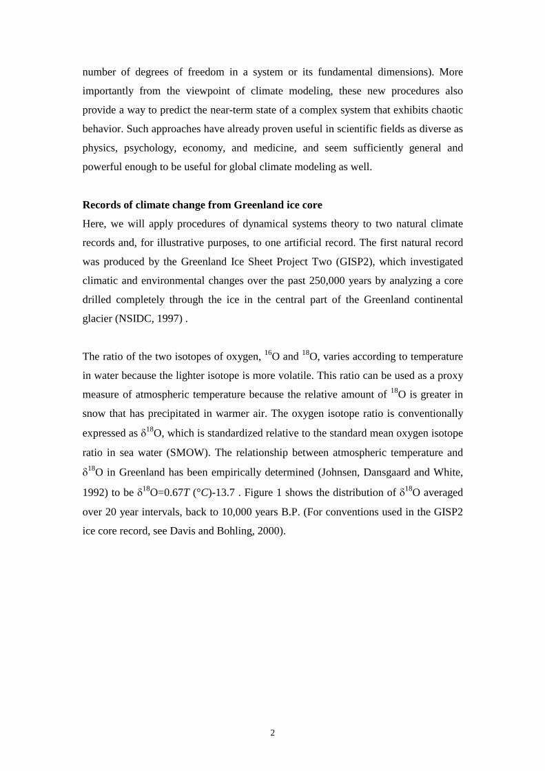
The ratio of the two isotopes of oxygen, 16O and 18O, varies according to temperature

in water because the lighter isotope is more volatile. This ratio can be used as a proxy

measure of atmospheric temperature because the relative amount of 18O is greater in

snow that has precipitated in warmer air. The oxygen isotope ratio is conventionally

expressed as �18O, which is standardized relative to the standard mean oxygen isotope

ratio in sea water (SMOW). The relationship between atmospheric temperature and

�18O in Greenland has been empirically determined (Johnsen, Dansgaard and White,

1992) to be �18O=0.67T (�C)-13.7 . Figure 1 shows the distribution of �18O averaged

over 20 year intervals, back to 10,000 years B.P. (For conventions used in the GISP2

ice core record, see Davis and Bohling, 2000).

2

Years B.P.

Del

ta 1

8O

-37.0

-36.5

-36.0

-35.5

-35.0

-34.5

-34.0

-33.5

-33.0

0 2000 4000 6000 8000 10000

Fig. 1. 20-year average record of �18O for the period of time 0-10 kyr BP from the

GISP2 ice core.

On cursory examination, the temperature record throughout the Holocene appears

chaotic, but closer examination shows trends of increasing or decreasing average

temperatures over specific intervals of time, such as during the last 200 years. Davis

and Bohling (2000) have characterized the GISP2 record of 20-year average �18O

values from a stochastic viewpoint. In contrast, we will examine the same record

regarding it as the output from a dynamic, nonlinear system complicated by random

influences.

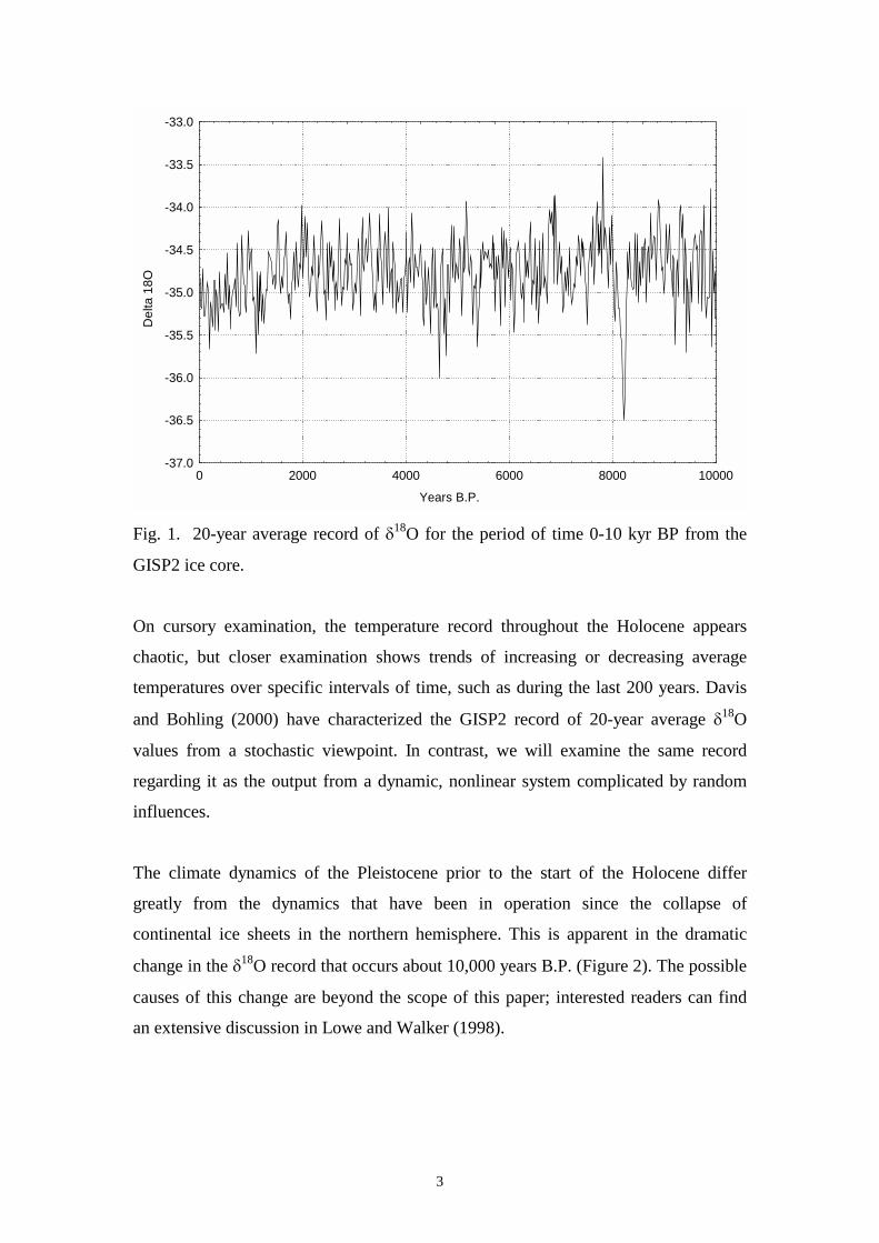
The climate dynamics of the Pleistocene prior to the start of the Holocene differ

greatly from the dynamics that have been in operation since the collapse of

continental ice sheets in the northern hemisphere. This is apparent in the dramatic

change in the �18O record that occurs about 10,000 years B.P. (Figure 2). The possible

causes of this change are beyond the scope of this paper; interested readers can find

an extensive discussion in Lowe and Walker (1998).

3

Years BP

Del

ta 1

8 O

-43

-41

-39

-37

-35

-33

-31

0 2000 4000 6000 8000 10000 12000 14000 16000

Fig. 2. 20-year average record of �18O for the period of time 0-16 kyr BP from the GISP2 ice core. The GISP2 record of 20-year average �18O extends back only a short time into the

Pleistocene (to 16,490 years B.P.) and consequently is not long enough to allow us to

assess climate dynamics of the pre-Holocene interval. However, there are more

extensive records of other constituents extracted from the GISP2 core, including Na,

NH4, K, Mg, Ca, Cl, NO3, and SO4. These variables can be combined into a single

composite variable by principal component analysis (Gorsuch, 1983), yielding a new

composite variable that is highly correlated with most of the measured constituents

and which expresses more than 76% of the variation in all of the original variables.

The record over time of this component is shown in Figure 3.

4

Years B.P.

FAC

TOR

1

-2

-1

0

1

2

3

4

5

10000 30000 50000 70000 90000

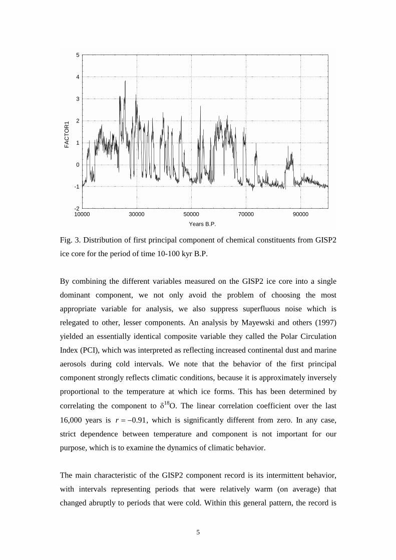
Fig. 3. Distribution of first principal component of chemical constituents from GISP2

ice core for the period of time 10-100 kyr B.P.

By combining the different variables measured on the GISP2 ice core into a single

dominant component, we not only avoid the problem of choosing the most

appropriate variable for analysis, we also suppress superfluous noise which is

relegated to other, lesser components. An analysis by Mayewski and others (1997)

yielded an essentially identical composite variable they called the Polar Circulation

Index (PCI), which was interpreted as reflecting increased continental dust and marine

aerosols during cold intervals. We note that the behavior of the first principal

component strongly reflects climatic conditions, because it is approximately inversely

proportional to the temperature at which ice forms. This has been determined by

correlating the component to �18O. The linear correlation coefficient over the last

16,000 years is , which is significantly different from zero. In any case,

strict dependence between temperature and component is not important for our

purpose, which is to examine the dynamics of climatic behavior.

91.0��r

The main characteristic of the GISP2 component record is its intermittent behavior,

with intervals representing periods that were relatively warm (on average) that

changed abruptly to periods that were cold. Within this general pattern, the record is

5

characterized by high-frequency, low-amplitude oscillations. Causes of the major

episodic alterations from relatively warm to cold and vice versa remain to be

established. Most likely, these changes are a consequence of both external and

internal influences that operated at a planetary scale. Possibly these long-term

variations in climatic temperature were due to orbital forcing (Imbrie and others,

1993) modulated by changes in circulation within the oceanic and atmospheric covers

of the Earth (Lowe and Walker, 1998).

The third record to be considered in this paper is artificial, the x-coordinate of the

realization of mathematical equations that describe the Lorenz system. This system of

equations was developed by Edward Lorenz by simplifying and linearizing

hydrodynamic equations as part of his research into weather patterns (Lorenz, 1963).

.

;

;

bZXYdtdZ

YrXXZdtdY

YXdtdX

��

����

��� ��

(1)

The Lorenz system operates in three-dimensional phase space – the space in which

variables describing the behavior of a dynamic system are entirely confined. The

parameter � is a Prandtl number, the parameter r is the ratio of the Rayleigh number

and critical Rayleigh number. The third parameter b is related to the horizontal wave

number of the system.

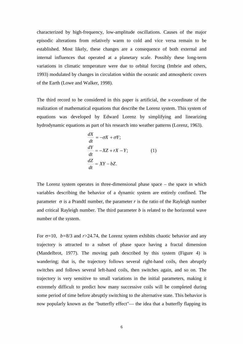
For �=10, b=8/3 and r>24.74, the Lorenz system exhibits chaotic behavior and any

trajectory is attracted to a subset of phase space having a fractal dimension

(Mandelbrot, 1977). The moving path described by this system (Figure 4) is

wandering; that is, the trajectory follows several right-hand coils, then abruptly

switches and follows several left-hand coils, then switches again, and so on. The

trajectory is very sensitive to small variations in the initial parameters, making it

extremely difficult to predict how many successive coils will be completed during

some period of time before abruptly switching to the alternative state. This behavior is

now popularly known as the "butterfly effect"— the idea that a butterfly flapping its

6

wings in Saint Petersburg can set in motion a complicated chain of events that

ultimately affects the weather in Kansas City.

Fig. 4. Trajectory of the Lorenz system.

When viewed in its full three dimensions as in Figure 4, the Lorenz system seems to

have no resemblance to the measures of climate recorded in the ice cores. However,

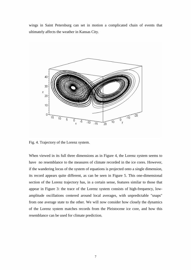
if the wandering locus of the system of equations is projected onto a single dimension,

its record appears quite different, as can be seen in Figure 5. This one-dimensional

section of the Lorenz trajectory has, in a certain sense, features similar to those that

appear in Figure 3: the trace of the Lorenz system consists of high-frequency, low-

amplitude oscillations centered around local averages, with unpredictable "snaps"

from one average state to the other. We will now consider how closely the dynamics

of the Lorenz system matches records from the Pleistocene ice core, and how this

resemblance can be used for climate prediction.

7

x

-25

-15

-5

5

15

25

# 1

# 51

# 10

1#

151

# 20

1#

251

# 30

1#

351

# 40

1#

451

# 50

1#

551

# 60

1#

651

# 70

1#

751

# 80

1#

851

# 90

1#

951

# 10

01#

1051

# 11

01#

1151

# 12

01#

1251

# 13

01#

1351

# 14

01#

1451

# 15

01#

1551

# 16

01#

1651

# 17

01

Fig. 5. x-coordinate of the Lorenz system. Horizontal axis is a discrete non-

dimensional time (�t=0.05).

Simple nonlinear prediction

Approaches stemming from dynamical systems theory allow us to make predictions

both in strictly deterministic systems that exhibit chaotic behavior (such as the Lorenz

system) and in systems which contain superimposed random noise. Different methods

of prediction are used in such systems (Weigend and Gershenfeld, 1994), but most of

them are based on the idea of the time decomposition of a single time series followed

by phase space reconstruction (Grassberger and Procassia, 1983).

First, following this approach we create a sequence of state vectors X(i) from the

available one-dimensional sequence, x(i):

))}1((),...,(),({)( ���� MLixLixixiX . (2)

Here, L is the "lag," or number of sampling intervals between successive components

of the delay vectors and M is the dimension of the delay vector. In other words, from

a one-dimensional sequence of measured values we construct a new sequence of M-

dimensional vectors X(i) which define some trajectory in M-dimensional space. A

8

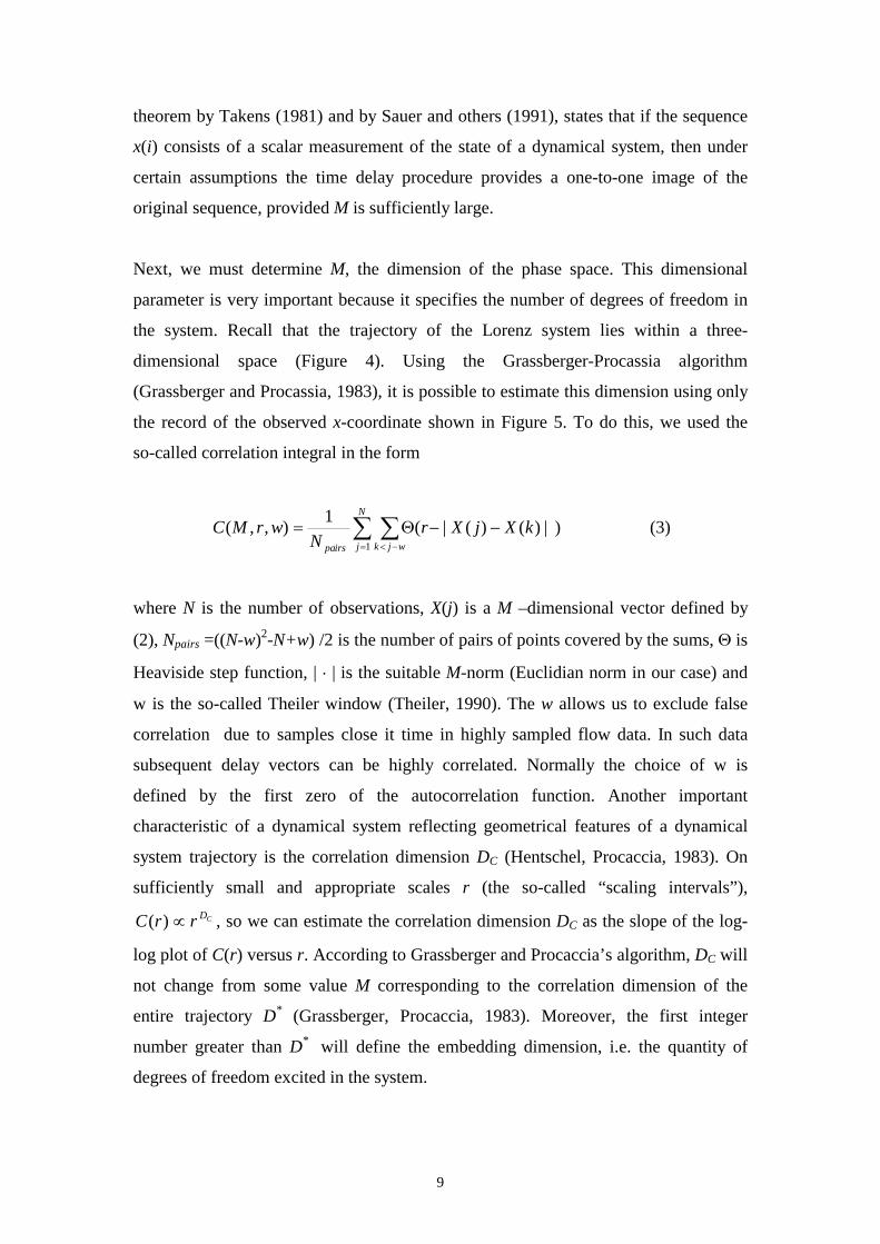
theorem by Takens (1981) and by Sauer and others (1991), states that if the sequence

x(i) consists of a scalar measurement of the state of a dynamical system, then under

certain assumptions the time delay procedure provides a one-to-one image of the

original sequence, provided M is sufficiently large.

Next, we must determine M, the dimension of the phase space. This dimensional

parameter is very important because it specifies the number of degrees of freedom in

the system. Recall that the trajectory of the Lorenz system lies within a three-

dimensional space (Figure 4). Using the Grassberger-Procassia algorithm

(Grassberger and Procassia, 1983), it is possible to estimate this dimension using only

the record of the observed x-coordinate shown in Figure 5. To do this, we used the

so-called correlation integral in the form

� �� ��

����

N

j wjkpairs

kXjXrN

wrMC1

|),)()(|(1),,( (3)

where N is the number of observations, X(j) is a M –dimensional vector defined by

(2), Npairs =((N-w)2-N+w) /2 is the number of pairs of points covered by the sums, � is

Heaviside step function, | � | is the suitable M-norm (Euclidian norm in our case) and

w is the so-called Theiler window (Theiler, 1990). The w allows us to exclude false

correlation due to samples close it time in highly sampled flow data. In such data

subsequent delay vectors can be highly correlated. Normally the choice of w is

defined by the first zero of the autocorrelation function. Another important

characteristic of a dynamical system reflecting geometrical features of a dynamical

system trajectory is the correlation dimension DC (Hentschel, Procaccia, 1983). On

sufficiently small and appropriate scales r (the so-called “scaling intervals”),

, so we can estimate the correlation dimension DCDrrC �)( C as the slope of the log-

log plot of C(r) versus r. According to Grassberger and Procaccia’s algorithm, DC will

not change from some value M corresponding to the correlation dimension of the

entire trajectory D* (Grassberger, Procaccia, 1983). Moreover, the first integer

number greater than D* will define the embedding dimension, i.e. the quantity of

degrees of freedom excited in the system.

9

So, for an arbitrary one-dimensional sequence it is possible to estimate the

dimensionality of an entire dynamical system, if such a system exists. The estimate of

the dimension of the phase space is also useful as a measure of the complexity of the

system.

The last step is prediction itself. Figure 6 shows, for illustrative purposes, a record of

the Lorenz system. To predict x(i+j) from the record at point i we first impose a

metric on the M-dimensional state space (in this instance, we have used simple

Euclidean distance as the metric) and find the k nearest neighbors of X(i) from the

past , where S is the set of indices of the k nearest neighbors. The

prediction is simply the average over the "future" X(l+j) of the neighbors X(l),

. In other words, we must consider that part of the phase space around

the predicted point and see what happens within this domain during the evolution of

the system (Figure 6). To obtain a prediction in the one-dimensional space of the

original data, we need only consider the first components of the delay-time vectors.

The prediction is then simply

SlillX �� ,:)(

kll ,...,, 21ll �

,)(1),( ��

��

Slpred jlx

kjix (4)

i.e., the average over the first components of “future” of the neighbors. The procedure

is described in detail in Farmer and Sidorovich (1987) and Hegger and others (1999).

10

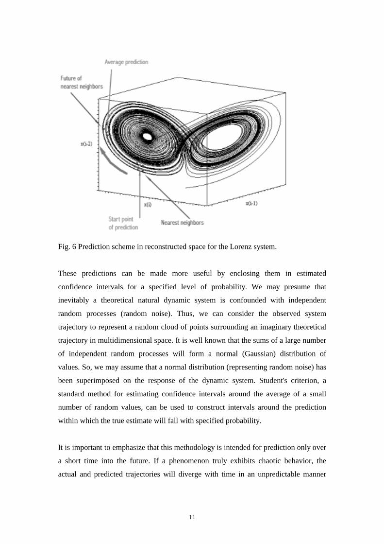
Fig. 6 Prediction scheme in reconstructed space for the Lorenz system.

These predictions can be made more useful by enclosing them in estimated

confidence intervals for a specified level of probability. We may presume that

inevitably a theoretical natural dynamic system is confounded with independent

random processes (random noise). Thus, we can consider the observed system

trajectory to represent a random cloud of points surrounding an imaginary theoretical

trajectory in multidimensional space. It is well known that the sums of a large number

of independent random processes will form a normal (Gaussian) distribution of

values. So, we may assume that a normal distribution (representing random noise) has

been superimposed on the response of the dynamic system. Student's criterion, a

standard method for estimating confidence intervals around the average of a small

number of random values, can be used to construct intervals around the prediction

within which the true estimate will fall with specified probability.

It is important to emphasize that this methodology is intended for prediction only over

a short time into the future. If a phenomenon truly exhibits chaotic behavior, the

actual and predicted trajectories will diverge with time in an unpredictable manner

11

because of the sensitivity of the system to the initial parameters. Long-term

predictions should be made only with extreme caution.

Examples of predictions

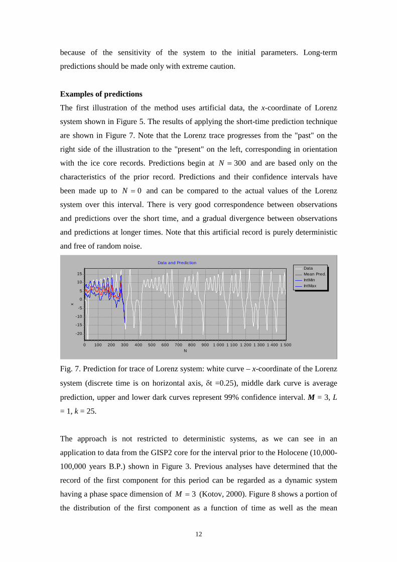
The first illustration of the method uses artificial data, the x-coordinate of Lorenz

system shown in Figure 5. The results of applying the short-time prediction technique

are shown in Figure 7. Note that the Lorenz trace progresses from the "past" on the

right side of the illustration to the "present" on the left, corresponding in orientation

with the ice core records. Predictions begin at N � 300 and are based only on the

characteristics of the prior record. Predictions and their confidence intervals have

been made up to N � 0 and can be compared to the actual values of the Lorenz

system over this interval. There is very good correspondence between observations

and predictions over the short time, and a gradual divergence between observations

and predictions at longer times. Note that this artificial record is purely deterministic

and free of random noise.

DataMean Pred.IntMinIntMax

Data and Prediction

N1 5001 4001 3001 2001 1001 0009008007006005004003002001000

x

15

10

5

0

-5

-10

-15

-20

Fig. 7. Prediction for trace of Lorenz system: white curve – x-coordinate of the Lorenz

system (discrete time is on horizontal axis, �t =0.25), middle dark curve is average

prediction, upper and lower dark curves represent 99% confidence interval. M = 3, L

= 1, k = 25.

The approach is not restricted to deterministic systems, as we can see in an

application to data from the GISP2 core for the interval prior to the Holocene (10,000-

100,000 years B.P.) shown in Figure 3. Previous analyses have determined that the

record of the first component for this period can be regarded as a dynamic system

having a phase space dimension of M � 3 (Kotov, 2000). Figure 8 shows a portion of

the distribution of the first component as a function of time as well as the mean

12

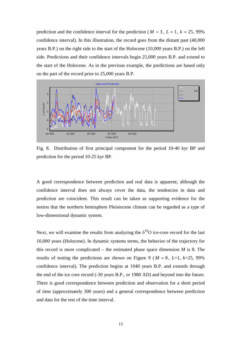
prediction and the confidence interval for the prediction ( M � 3 , L � 1 , k � 25 , 99%

confidence interval). In this illustration, the record goes from the distant past (40,000

years B.P.) on the right side to the start of the Holocene (10,000 years B.P.) on the left

side. Predictions and their confidence intervals begin 25,000 years B.P. and extend to

the start of the Holocene. As in the previous example, the predictions are based only

on the part of the record prior to 25,000 years B.P.

DataMean PrIntMinIntMax

40 00035 000

8

ed.

Data and Prediction

Y ears B.P.30 00025 00020 00015 00010 000

1-st

fac

tor

3

2

1

0

-1

Fig. 8. Distribution of first principal component for the period 10-40 kyr BP and

prediction for the period 10-25 kyr BP.

A good correspondence between prediction and real data is apparent; although the

confidence interval does not always cover the data, the tendencies in data and

prediction are coincident. This result can be taken as supporting evidence for the

notion that the northern hemisphere Pleistocene climate can be regarded as a type of

low-dimensional dynamic system.

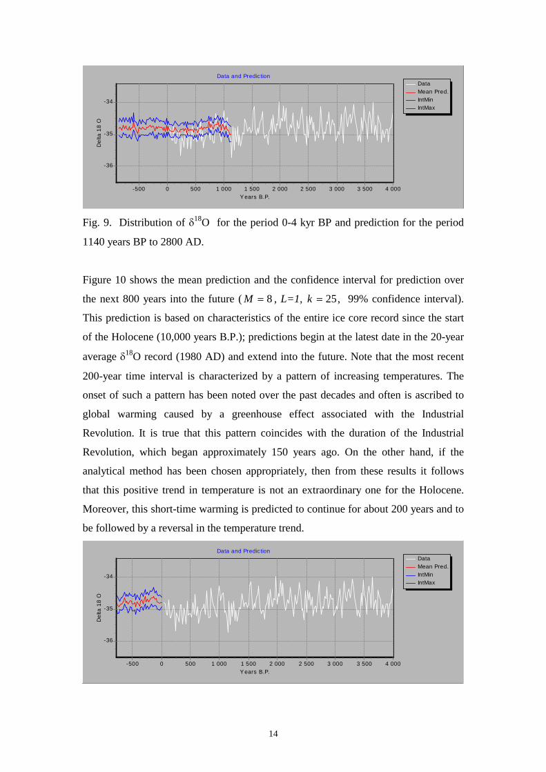
Next, we will examine the results from analyzing the �18O ice-core record for the last

10,000 years (Holocene). In dynamic systems terms, the behavior of the trajectory for

this record is more complicated – the estimated phase space dimension M is 8. The

results of testing the predictions are shown on Figure 9 ( M � , L=1, k=25, 99%

confidence interval). The prediction begins at 1040 years B.P. and extends through

the end of the ice core record (-30 years B.P., or 1980 AD) and beyond into the future.

There is good correspondence between prediction and observation for a short period

of time (approximately 300 years) and a general correspondence between prediction

and data for the rest of the time interval.

13

DataMean Pred.IntMinIntMax

Data and Prediction

Y ears B.P.4 0003 5003 0002 5002 0001 5001 0005000-500

Del

ta 1

8 O

-34

-35

-36

Fig. 9. Distribution of �18O for the period 0-4 kyr BP and prediction for the period

1140 years BP to 2800 AD.

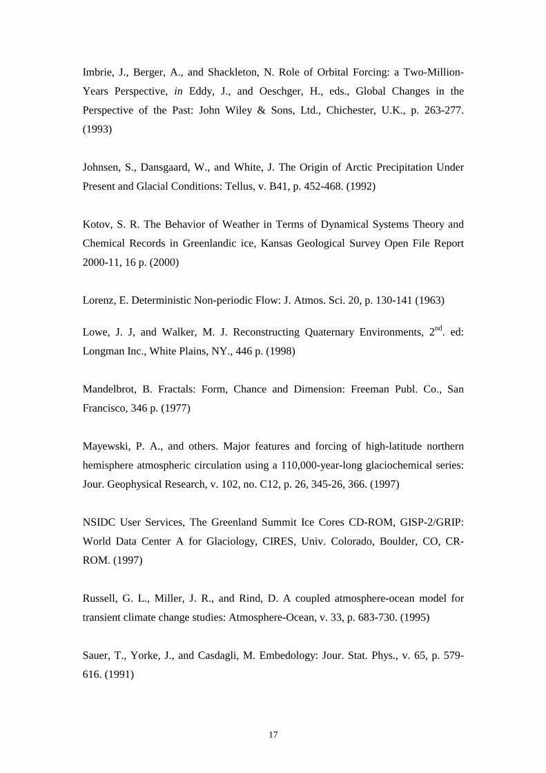
Figure 10 shows the mean prediction and the confidence interval for prediction over

the next 800 years into the future ( M � 8 , L=1, k � 25 , 99% confidence interval).

This prediction is based on characteristics of the entire ice core record since the start

of the Holocene (10,000 years B.P.); predictions begin at the latest date in the 20-year

average �18O record (1980 AD) and extend into the future. Note that the most recent

200-year time interval is characterized by a pattern of increasing temperatures. The

onset of such a pattern has been noted over the past decades and often is ascribed to

global warming caused by a greenhouse effect associated with the Industrial

Revolution. It is true that this pattern coincides with the duration of the Industrial

Revolution, which began approximately 150 years ago. On the other hand, if the

analytical method has been chosen appropriately, then from these results it follows

that this positive trend in temperature is not an extraordinary one for the Holocene.

Moreover, this short-time warming is predicted to continue for about 200 years and to

be followed by a reversal in the temperature trend.

DataMean Pred.IntMinIntMax

Data and Prediction

Y ears B.P.4 0003 5003 0002 5002 0001 5001 0005000-500

Del

ta 1

8 O

-34

-35

-36

14

Fig. 10. Distribution of �18O for the period 0-4 kyr BP and prediction for 800 years

into the future.

Conclusions

Traditional models of global climate change are extremely complicated, rely on a

number of fundamental assumptions, and are difficult and costly to operate. Perhaps

most troublesome is the brevity of the historical record of climate on which the

models are conditioned. However, records of various constituents measured in

Greenland ice cores provide information about past variations in climate over

thousands of years before the present which can be used to help understand better the

processes of global climate change. Methods for reconstructing the entire

multidimensional trajectory of a process from its one-dimensional sequence of

measured values allows us to estimate important characteristics of dynamic systems

such as the number of degrees of freedom or the true dimensionality of the system.

The dimensionality reflects the number of independent variables in a system and must

be taken into account in the construction of a global climate model. In addition, this

approach permits us to make short-term predictions of important climatic variables.

The main characteristic of the 90,000 years that preceded the Holocene is the

intermittent behavior of the climate. Periods that were relatively warm (on average)

were abruptly followed by periods of intense cold. Within these relatively warm or

cold intervals, temperatures varied through high-frequency, low-amplitude

oscillations. Described in dynamic system terms, the climate behaved as a dynamical

system with 3 degrees of freedom. We obtain a good correspondence between

predicted behavior and reality by modeling climate as a low-dimensional dynamical

system over this period of time. The same characteristics are exhibited by a Lorenz

system – the simplest nonlinear deterministic model that can be applied. Such a

system has 3 degrees of freedom and demonstrates high-frequency oscillations with

unpredictable "snaps" from one space domain to another.

In terms of dynamical systems, the behavior of the climatic record in the Holocene is

more complicated – the dimensionality of the phase space M is 8. Estimates of

temperature based on a dynamical system model indicate that a positive trend in

15

temperature over a 200-year period is not unexpected for the Holocene. Predictions

based on the characteristics of the Holocene and extending into the future indicate that

the present short-term warming trend may continue for at least 200 years and be

followed by a reverse in the temperature trend.

Acknowledgments.

The author would like to acknowledge the help of Dr. G. Bohling with the editing of

text. Especially the author expresses his gratitude to Dr. J. Davis for valuable remarks

and proof-reading of the article.

References.

Davis, J. C., and Bohling, G. The Search for Patterns in Ice Core Temperature Curves,

in Geological Constraints on Global Climate, edited by L.C.Gerhard, W.E.Harrison,

and B.M.Hanson, AAPG, scheduled for publication in 2000.

Farmer, J. D., and Sidorowich, J. J. Predicting Chaotic Time Series: Physical Review

Letters, v. 59, no. 8, p. 845-848. (1987)

Gorsuch, R. Factor Analysis: L. Erlbaum Associated, Hillsdale, NJ, 452 p. (1983)

Grassberger, P., and Procassia, I. Characterization of Strange Attractors: Phys. Rev.

Lett., v. 50, no. 5, p. 346-349. (1983)

Hansen, J. G., and others. Efficient Three-Dimensional Global Models for Climate

Studies: Models I and II: Monthly Weather Review, v. 11, p. 609-662. (1983)

Hegger, R., Kantz, H., and Schreiber, T. Practical Implementation of Nonlinear Time

Series Methods: The TISEAN Package: Chaos, v. 9, no. 2, p. 413-435 (1999)

Hentschel H., Procaccia I. The Infinite Number of Generalized Dimensions of

Fractals and Strange Attractors // Physica 8D, 435-444 (1983)

16

Imbrie, J., Berger, A., and Shackleton, N. Role of Orbital Forcing: a Two-Million-

Years Perspective, in Eddy, J., and Oeschger, H., eds., Global Changes in the

Perspective of the Past: John Wiley & Sons, Ltd., Chichester, U.K., p. 263-277.

(1993)

Johnsen, S., Dansgaard, W., and White, J. The Origin of Arctic Precipitation Under

Present and Glacial Conditions: Tellus, v. B41, p. 452-468. (1992)

Kotov, S. R. The Behavior of Weather in Terms of Dynamical Systems Theory and

Chemical Records in Greenlandic ice, Kansas Geological Survey Open File Report

2000-11, 16 p. (2000)

Lorenz, E. Deterministic Non-periodic Flow: J. Atmos. Sci. 20, p. 130-141 (1963)

Lowe, J. J, and Walker, M. J. Reconstructing Quaternary Environments, 2nd. ed:

Longman Inc., White Plains, NY., 446 p. (1998)

Mandelbrot, B. Fractals: Form, Chance and Dimension: Freeman Publ. Co., San

Francisco, 346 p. (1977)

Mayewski, P. A., and others. Major features and forcing of high-latitude northern

hemisphere atmospheric circulation using a 110,000-year-long glaciochemical series:

Jour. Geophysical Research, v. 102, no. C12, p. 26, 345-26, 366. (1997)

NSIDC User Services, The Greenland Summit Ice Cores CD-ROM, GISP-2/GRIP:

World Data Center A for Glaciology, CIRES, Univ. Colorado, Boulder, CO, CR-

ROM. (1997)

Russell, G. L., Miller, J. R., and Rind, D. A coupled atmosphere-ocean model for

transient climate change studies: Atmosphere-Ocean, v. 33, p. 683-730. (1995)

Sauer, T., Yorke, J., and Casdagli, M. Embedology: Jour. Stat. Phys., v. 65, p. 579-

616. (1991)

17

Takens, F. Detecting Strange Attractor in Turbulence: Lecture Notes in Mathematics,

v. 898, p. 366-381. (1981)

Theiler J. Spusious Dimension from Correlation Algorithms Applied to Limited

Time-Series Data // J. Opt. Soc. Amer. A7, 1055 (1990)

Weigend, A. S., and Gershenfeld, N. A., eds. Time Series Prediction: Addison-

Wesley, Reading, MA, 643 p. (1994)

18